The 83rd Annual Conference of the Agricultural Economics Society

Dublin

30th March to 1st April 2009

Optimal Control of Spreading Biological Invasions: For How Long Should We Apply the Brake?

Luis R Carrascoa,b, Alan MacLeodb, Jon D Knighta, Richard Bakerb

and John D Mumforda aImperial College London, Centre for Environmental Policy, Exhibition Road,

London, SW7 2AZ, United Kingdom bCentral Science Laboratory, Sand Hutton, York, YO41 1LZ, United Kingdom

Emails: roman.carrasco@imperial.ac.uk, a.macleod@csl.gov.uk, j.d.knight@imperial.ac.uk, r.baker@csl.gov.uk, j.mumford@imperial.ac.uk.

Copyright 2009 by Luis Roman Carrasco, Alan MacLeod, Jon D Knight, Richard Baker and John D Mumford. All rights reserved. Readers may make verbatim copies of this document for non-commercial purposes by any means, provided that this copyright notice appears on all such copies.

Abstract

Identifying the optimal switching point between different invasive alien species (IAS) management policies is a very complex task and policy makers are in need of modelling tools to assist them. In this paper we develop an optimal control bioeconomic model to estimate the type of optimal policy and switching point of control efforts against a spreading IAS. We apply the models to the case study of Colorado potato beetle in the UK. The results demonstrate that eradication is optimal for small initial sizes of invasion at discovery. High capacity of the agency to reduce spread velocity for several years leads to smaller total overall costs of invasion and makes eradication optimal for larger sizes of initial invasion. In many cases, it is optimal to switch from control to acceptance within the time horizon. The switching point depends on the capacity of the agency, initial size of invasion, spread velocity of the IAS and the ratio of unit cost of damage and removal. We encourage the integration of the dispersal patterns of the invader and the geometry of the invasion in the theoretical development of the economics of IAS invasion management.

Keywords: barrier zone, biosecurity, dynamic optimization, eradication, Leptinotarsa decemlineata, pest risk analysis, reaction-diffusion.

JEL codes: Q1; Q28; Q57

Introduction

The introduction of invasive alien species (IAS) is one of the main causes of the loss

of global biodiversity. IAS lead to extinction of vulnerable native species through

predation, grazing, competition and habitat alteration (Mack et al., 2000). In addition,

IAS pose great costs to agricultural production, inflicting an increase in pest

management expenditures, yield reduction, losses of consumers and producers

welfare and loss of export markets.

The different stages of the IAS invasion are entry, establishment and spread.

Depending on which stage the invasion is at, these different management decisions

would need to be taken by government agencies in charge of managing IAS

invasions: prevention, eradication, containment, slowing down and/or acceptance of

the invasion1. Identifying the optimal policy and switching point between different

management policies is a very complex task and the government agencies are in need

of modelling tools to assist them. Bioeconomic modelling of IAS management

attempts to facilitate those decisions by estimating the optimal policy combination

that minimises the total costs of removal and total costs of damage caused by the

invasion for a specific time horizon.

Great insight has been gained on the bioeconomics of IAS management in recent

years. Analytical models have been devoted to the optimal allocation of resources for

preventative measures (Horan, et al., 2002) or after the IAS has been established in

order to determine when eradication is the optimum policy (Eiswerth and Van

Kooten, 2002; Olson and Roy, 2002; Odom et al., 2003; Burnett et al., 2007). Other

approaches more integrative of the invasion stages have focused on assessing the

optimal trade off between exclusion and control efforts (Leung et al. 2002; Olson and

Roy, 2005; Kim et al. 2006; Finnoff et al., 2007).

1 We define the following IAS management measures as follows: (i) prevention: aimed at reducing the probability of entry and establishment of an IAS; (ii) eradication: aimed at driving the population of the invader to extinction; (iii) containment: aimed at maintaining the invasion at a constant size; (iv) slowing down: aimed at reducing the spread velocity of the invasion whilst allowing it to expand its range; (v) acceptance: to stop managing the invasion and to allow it spread at its natural spread velocity. In this paper, any management measure applied to the invasion after its establishment will be referred to as a “control measure”.

These modelling approaches have largely concentrated on IAS population dynamics

instead of using theoretical spread models for IAS (e.g. see spread models by: Fisher,

1937; Skellman, 1951; Andow et al., 1990; Shigesada, 1995). Thus, few bioeconomic

analytical models take into account the geometry of the invasion. Instead,

demographic models are in some cases employed as substitutes for spread models

(e.g. logistic growth model). However, demographic models alone are unlikely to

provide accurate predictions of invasion spread rates because, in order to relate

population growth to spread velocity, it is necessary to take into account the spatial

dispersal patterns of the invader (Higgins and Richardson, 1996). Some notable

exceptions of bioeconomic models that consider the dispersal patterns of the invader

are those that incorporate the spread predictions of reaction-diffusion (R-D) models

(constant asymptotic spread velocity) into the management of invasions using barrier

zones (e.g. Sharov and Liebhold, 1998; Sharov, 2004; Cacho et al., 2008)2.

R-D models (Fisher, 1937, Skellman, 1951) are probably the most widely used IAS

spread models and have been applied successfully to predict invasion rates from

animal species (Levin, 1992). R-D models are partial differential equations where

random diffusion in a homogeneous environment is assumed. The main parameters

are ε, the intrinsic rate of population growth and D, the diffusivity of the population.

For instance the Skellman model is of the form: 2 2

2 2

n n nD nt x y

ε⎛ ⎞∂ ∂ ∂

= + +⎜ ⎟∂ ∂ ∂⎝ ⎠, (1)

where the left hand side in equation (1) represents the change in population density

(n) at time (t) and spatial coordinates (x,y) that is caused by random diffusion (first

term of the right hand side) and local population growth (second term of the right

hand side). The solution of the R-D model is:

4c Dε= , (2)

by which spread is predicted to follow a continuous expansion at an asymptotically

constant radial velocity represented by c.

2 A barrier zone is defined as the area bordering the expansion front of the invasion where management activities are carried out with the aim of reducing the velocity or even to lead to eradication of the invasion. For example, moving barrier zones were employed for the eradication of the boll weevil (Anthonomous grandis) in the United States (Sharov, 2004).

Case study: Risk of Colorado potato beetle invasion in the UK

The Colorado potato beetle (CPB) Leptinotarsa decemlineata (Say) (Insecta:

Coleoptera: Chrysomelidae) is the most important pest of potato (Solanum tuberosum)

in most areas of North America. CPB also affects other Solanum species widely

present in the UK. Adults are capable of flying up to 3km and their dispersal can also

be assisted by weather events and commercial traffic (Bartlett, 1980; Waage, et al.,

2005). For instance, CPB adults arrived en masse from Poland and Germany into

southern Sweden (Wiktelius, 1981). CPB was inadvertently introduced in Western

Europe apparently during World War I. As a result, CPB is now established in large

areas of Europe with the exception of the United Kingdom (UK), Ireland, Sweden,

Finland and some Spanish and Portuguese islands (Heikkila and Peltola, 2004). The

European and Mediterranean Plant Protection Organisation (EPPO) declares CPB as

present in the EPPO region but not widely distributed and recommends it be

controlled as a quarantine pest (EPPO, 2009). Thus most of the uninfested regions

present protected zones against invasion by CPB.

The UK has adopted a successful policy of prevention and eradication of any breeding

colonies of CPB since 1877. Breeding colonies have been eradicated during the years

1901-02, 1933-34, 1946-52 and 1976-77 and non-breeding individuals are intercepted

in imported vegetable produce almost every year (Bartlett, 1980). These interceptions

reflect the permanent risk that CPB represents to the UK potato industry. This risk is

increasing: under climate change projections the potential range for the development

of CPB in the UK is estimated to increase by 102% (Baker et al., 1996). Hence an

increase in the occurrence of breeding colonies and corresponding eradication

campaigns is expected.

Whereas the benefits of living without CPB have been demonstrated in the cases of

the UK (Mumford et al., 2000; Waage et al., 2005) and Finland (Heikkila and Peltola,

2004), eradication campaigns are very costly and it is necessary to know how long

they are justifiable for.

In this paper, we develop a bioeconomic optimal control model where an already

established IAS spreads following R-D and a moving barrier zone is considered for

the management of the invasion. We apply the model to the case study of potential

CPB invasion in the UK. We build upon the work of Sharov and Liebhold (1998)

using instead an optimal control approach and imposing a constraint on the control

measures. We consider four main scenarios: Scenario A (C): introduction at the centre

of the susceptible range and spread under current climate conditions (climate change

projections); scenario B (D): introduction nearby the coast and spread under current

climate conditions (climate change projections). The outcome of the study is a

bioeconomic model to identify the optimal type of policy and time at which to stop

control efforts against an IAS invasion.

Methodology

Policy problem: when to stop control measures

We consider the optimal control problem: whether to control or accept an already

established IAS that is spreading following a R-D model (equation (2)). A

homogeneous landscape is assumed. Therefore, the asymptotic radial velocity of

spread c is constant in every direction, leading to a circular (or fraction of circle)

invasion front that is centred at the initial establishment point. In addition, the total

area susceptible to be invaded (susceptible range) is assumed to be well approximated

by a circle or fraction of circle. Hence, the circular shape of the invasion front holds

for all time t. The control variable of the problem (variable over which the agency has

the capacity to influence) is u, aimed reduction of spread velocity. u is the

consequence of removal activities by a moving barrier zone. The state variable is x,

radius of the area invaded. At the moment of discovery the invasion has a size of x =

x0 due to undetected spread. We assume that c is constant for all x > 0 and c = 0 for x

= 0 (eradication) and x = xmax (total susceptible range is invaded).

The problem for the government agency is to minimise (transformed into a

maximisation problem by multiplying the objective function by minus one) the net

present value (NPV) of the total overall costs (total costs of removal of the invasion

and the total costs of damages caused by the IAS in the remaining area invaded,

L(x,u)):

Maximise L where . (3) ( ) ( )( ) ( )( )(0

, ,T

r tL x u e D x t R x t u dt− ⋅= − +∫ )

Subject to:

x c ut∂

= −∂

(4)

max0 u u≤ ≤ (5)

max0 x x≤ ≤ (6)

( ) 00x x= , (7)

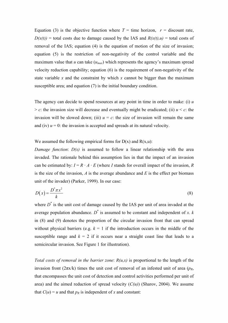
Equation (3) is the objective function where T = time horizon, r = discount rate,

D(x(t)) = total costs due to damage caused by the IAS and R(x(t),u) = total costs of

removal of the IAS; equation (4) is the equation of motion of the size of invasion;

equation (5) is the restriction of non-negativity of the control variable and the

maximum value that u can take (umax) which represents the agency’s maximum spread

velocity reduction capability; equation (6) is the requirement of non-negativity of the

state variable x and the constraint by which x cannot be bigger than the maximum

susceptible area; and equation (7) is the initial boundary condition.

The agency can decide to spend resources at any point in time in order to make: (i) u

> c: the invasion size will decrease and eventually might be eradicated; (ii) u < c: the

invasion will be slowed down; (iii) u = c: the size of invasion will remain the same

and (iv) u = 0: the invasion is accepted and spreads at its natural velocity.

We assumed the following empirical forms for D(x) and R(x,u):

Damage function: D(x) is assumed to follow a linear relationship with the area

invaded. The rationale behind this assumption lies in that the impact of an invasion

can be estimated by: I = R · A · E (where I stands for overall impact of the invasion, R

is the size of the invasion, A is the average abundance and E is the effect per biomass

unit of the invader) (Parker, 1999). In our case:

( )* 2D xD xkπ

= (8)

where D* is the unit cost of damage caused by the IAS per unit of area invaded at the

average population abundance. D* is assumed to be constant and independent of x. k

in (8) and (9) denotes the proportion of the circular invasion front that can spread

without physical barriers (e.g. k = 1 if the introduction occurs in the middle of the

susceptible range and k = 2 if it occurs near a straight coast line that leads to a

semicircular invasion. See Figure 1 for illustration).

Total costs of removal in the barrier zone: R(u,x) is proportional to the length of the

invasion front (2πx/k) times the unit cost of removal of an infested unit of area (pR,

that encompasses the unit cost of detection and control activities performed per unit of

area) and the aimed reduction of spread velocity (C(u)) (Sharov, 2004). We assume

that C(u) = u and that pR is independent of x and constant:

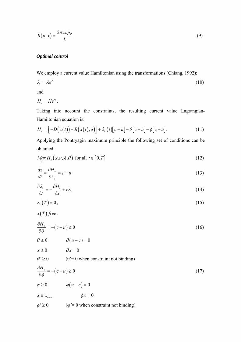
( ) 2, Rxup

R u xk

π= . (9)

Optimal control

We employ a current value Hamiltonian using the transformations (Chiang, 1992): rt

c eλ λ= (10)

and rt

cH He= .

Taking into account the constraints, the resulting current value Lagrangian-

Hamiltonian equation is:

( )( ) ( )( ) ( )[ ] [ ] [ ],c cH D x t R x t u t c u c u cλ θ φ⎡ ⎤= − − + − − − − −⎣ ⎦ u . (11)

Applying the Pontryagin maximum principle the following set of conditions can be

obtained:

( ), , ,cuMax H x u λ θ for all [ ]0,t T∈ (12)

c

c

Hdx c udt λ

∂= = −∂

(13)

c cc

H rt xλ λ∂ ∂

= − +∂ ∂

(14)

( ) 0c Tλ = ; (15)

( )x T free .

( ) 0cHc u

θ∂

= − − ≥∂

(16)

0θ ≥ ( ) 0u cθ − =

0x ≥ 0xθ =

' 0θ ≥ (θ’= 0 when constraint not binding)

( ) 0cHc u

φ∂

= − − ≥∂

(17)

0φ ≥ ( ) 0u cφ − =

0xφ = maxx x≤

' 0φ ≥ (φ’= 0 when constraint not binding)

Equation (12) indicates that the optimal control u*(t) must maximise the Lagrangian-

Hamiltonian for all t within the time horizon considered; (13) is the equation of

motion for x; (14) is the equation of motion of the costate variable λc modified for the

current value Hamiltonian; (15) are the transversality conditions for a vertical

terminal line at t = T; equations (16) and (17) are the conditions due to the

constrained state variable (equation (6)). The complementary-slackness conditions

state that θ and φ, the Lagrangian multipliers, will be zero unless x = 0 and x = xmax

respectively (the state constraints become binding).

We initially assume that constraints (16) and (17) are not binding for all t and solve

the problem as an unconstrained problem. Given that Hc is linear in the control

variable u, we obtain a bang-bang solution for u (Clark, 1990). ∂Hc/∂u is called the

switching function and is referred to as σ. To maximise Hc, the boundary solution u*=

0 (acceptance of invasion) should be chosen if σ is negative and u*= umax will be

chosen if σ is positive. Only if σ = 0 for a positive interval of time, the Hamiltonian

does not depend of u and we obtain a singular solution. The optimal control is

described as:

max*

00 undetermined0 0

c

uH

uu

> ⎧ ⎫⎧ ⎫∂ ⎪ ⎪ ⎪= ⇒ =⎨ ⎬ ⎨∂ ⎪ ⎪ ⎪<⎩ ⎭ ⎩ ⎭

⎪⎬⎪

(18)

where

2c Rc c

H xpRu u k

πσ λ λ

∂ ∂= = − − = − −

∂ ∂. (19)

If there is a singular solution (σ = 0) u* (0 < u* < uB), equation (19) indicates that the

marginal benefit of reducing the size of the invasion (λc) must equal the marginal

costs that led to such reduction. If there is no singular solution, the optimal control

contains only the extreme levels of control and there will be as many switches (from

u*= umax to u* = 0 or vice versa) as the number of roots that σ has.

Applying the conditions of the maximum principle we identified (see Appendix 1)

five critical points in time determining the optimal control path: τ, the optimal time to

switch policy (solution of the unconstrained problem); terad, the time when the

invasion is eradicated (constraint (16) is binding); txmax the time when all the

susceptible range is invaded (constraint (17) is binding); and the starting (t = 0) and

final time T of the time horizon. τ is obtained by solving for t in equation (20) when σ

= 0:

( ) ( )max 0 2 2

1 2 r t TRp ct tu x e

k r rσ π −Ψ⎛ ⎞= − − + + −⎜ ⎟

⎝ ⎠1

Ψ (20)

where:

( ) ( )* * *max max max 0Rc D D rt p ru D u rtu rxΨ = + + − + −

and σ has only one root.

terad and txmax are obtained by solving for t in equation (21) when x = 0 and x = xmax

respectively:

( )max 0x c u t x= − + (21)

It is not possible to check for singular solutions analytically. We employed numerical

methods instead to check that σ does not vanish for a positive interval of time. We

ruled out singular solutions and the optimal control was considered a normal bang-

bang control (Lewis and Syrmos, 1995). We can summarise the different type of

optimal control policies into five scenarios (assuming that we initially control, then

accept the invasion rather than accepting first, then controlling the invasion):

Case ACase BCase CCase DCase E

⎧ ⎫⎪ ⎪⎪ ⎪⎪ ⎪⎨ ⎬⎪ ⎪⎪ ⎪⎪ ⎪⎩ ⎭

xmax

xmax

xmax

xmax

0 ( , , )0 ( , , 0 ( , )0 ( , )( , , ) 0

erad

erad

erad

erad

t t TT t tt Tt Tt t T

ττ

ττ

τ

< <⎧ ⎫⎪ ⎪< <⎪ ⎪⎪ ⎪< ≤⎨ ⎬⎪ ⎪< ≤⎪ ⎪⎪ ⎪< <⎩ ⎭

)

*max

*max

*max

*max

0

u u

u u

u u

u uu

⎧ ⎫=⎪ ⎪

=⎪ ⎪⎪ ⎪⇒ =⎨ ⎬⎪ ⎪=⎪ ⎪⎪ ⎪=⎩ ⎭

for xmax

00000

erad

tt Tt tt tt T

τ≤ ≤⎧ ⎫⎪ ⎪≤ ≤⎪ ⎪⎪ ⎪≤ ≤⎨ ⎬⎪ ⎪≤ ≤⎪ ⎪⎪ ⎪≤ ≤⎩ ⎭

and{ }* 0u = for

(22) xmax

erad

t T

t tt t

τ < <−< << <−

TT

⎧ ⎫⎪ ⎪⎪ ⎪⎪ ⎪⎨ ⎬⎪ ⎪⎪ ⎪⎪ ⎪⎩ ⎭

The type of optimal control policies are: Case A where u = umax until t = τ; after that

we accept the invasion that will continue spreading. In case B, we control the invasion

during the entire time period and not all the susceptible area is occupied. In case C,

we control the invasion until the entire susceptible area is occupied and then we

accept it. In case D, the control is applied until eradication is achieved; then control

stops. In case E, we accept the invasion without any attempt to control it.

Model parameterisation

We estimated pR from the eradication campaign against CPB in 1976-77 in Thanet

(Kent, UK) where a colony occupied an area of 184m2 within a 19ha field. This

campaign involved the following activities within a radius of 1.6 km: several aircraft

and terrestrial insecticide spraying, compensation to farmers for the destruction of

crops, use of bait crops and multiple inspections by Ministry officers (Bartlett, 1980).

We assumed a homogeneous distribution of potato production through the landscape.

The total costs of removal, (in 2005 pounds) added up to £102070 (119.21 £/km2 of

landscape treated, Table 1). On the other hand, the unit cost due to damages of an

invaded ha of potato (D*) add up to 53.54 £/ha (Waage et al., 2005). These include

costs due to inspection, insecticide application, yield losses and export losses. We

expressed those costs per km2 of landscape (to match with the units of the predictions

of the R-D model). The asymptotic velocity of spread (c) was estimated using

equation (2) (values of parameters in Table 1). Given that potato and other Solanum

species are very widespread in the UK, we assumed that in all the areas where there

where adequate climatic conditions for the development of CPB, Solanum species

were present. The maximum radius for the four main scenarios considered (circular or

semicircular invasion under current climate conditions and climate change

projections) was estimated assuming a circle and semicircle of equivalent area to the

area of the susceptible range for CPB in the UK (79500 km2 for temperatures from

1960-90 and 160700 km2 for climate change projections for 2060-70) (Baker, et al.,

1996). In addition, we assumed that the plant protection agency would be able to

deploy control outlays so as to maintain a maximum spread velocity reduction of 10

km/year (umax).

Results

In many cases, eradication is the only option considered by government agencies

unless the invasion is too large, in which case acceptance is the policy option adopted.

There is a need to know when to attempt eradication and if there are other policies

like slowing down the invasion that are optimal before the final acceptance of the

invasion. For all parameters combinations, the optimal policy corresponded to some

form of control after discovery and then acceptance. As expected, it was never

optimal to accept first the invasion and then control for it after the switching point.

Effect of initial size of invasion and agency’s maximum spread velocity reduction

capability on the type of optimal policy

The model identified eradication policies against CPB in the UK as optimal for low

initial infestation sizes and for high agency’s maximum spread velocity reduction

capability (umax) (Figure 2). On the other hand, for agencies incapable of deploying an

invasion size reducing campaign, it was not optimal to accept CPB without adopting a

slowing down policy for a period of time before the final acceptance of the invasion

(Figure 2). The required umax that makes eradication optimal increased with increasing

initial sizes of invasion. For instance, an initial invasion of 30 km (75 km) radius

would need at least an umax of 5 km/year (7 km/year) for eradication to be optimal

(Figure 2).

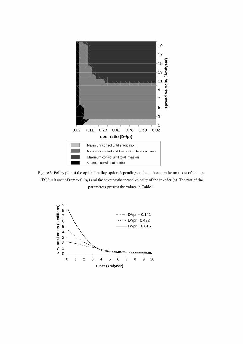
Effect of the unit cost ratio and the spread velocity on the type of optimal policy

Whereas for the case of CPB a policy of acceptance without control was not optimal,

that policy would be optimal for other IAS presenting a lower unit cost ratio (D*/pR)

(Figure 3). That is, IAS that are very costly to remove and at the same time do not

inflict relevant damage costs per unit of invaded area (costs ratio < 0.04), should be

left to spread naturally, independently of their spread velocity. On the other hand,

slow spreading invaders (up to 2.5 km/year) should be eradicated independently of

their unit cost ratio (as long as cost ratio > 0.04 and umax = 10 km/year). For spread

velocities below umax it was optimal to control until a switching point and then to

accept the invasion. The time at which the switch occurred was closer to the starting

point of the time horizon with decreasing unit cost ratios. For higher unit cost ratios

and IAS spreading faster than umax, control efforts should occur for the entire time

horizon (Figure 3).

Effects of climate change, introduction point and spread velocity

The effect of climate change implied larger susceptible ranges of invasion. This had

no effect at low spread velocities (3.1 km/year) because the total susceptible range

was not occupied (Table 2). By contrast, when higher spread velocities (50 km/year

for historical spread rates) led to total susceptible range occupation within the time

horizon, the size range and shape of the invasion had an effect on the total overall

cost, type of optimal policy and switching point (compare columns 3rd and 4th to 7th

and 8th in Table 2).

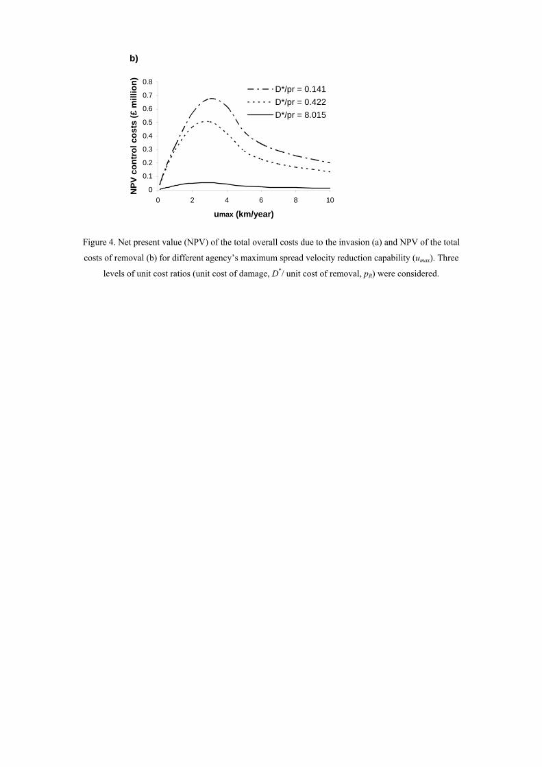
Effect of umax on total overall costs and total removal costs

umax had a large effect on the success of the optimal management policy (Figure 4a).

The total overall costs due to the invasion were a decreasing function of umax,

indicating the importance of being able to carry out large and effective campaigns

through time. The peak of total costs of removal occurred for umax close to and below

the invasion spread (Figure 4b). That is, it is optimal to control for long periods of

time if we are capable to slow spread considerably. On the other hand, if umax is very

low, acceptance occurs at an early stage resulting in less total costs of removal.

Equally, if umax is high, we will achieve eradication soon and the total costs of

removal are also lower (Figure 4b).

Effect of spread velocity on total overall costs and total control costs

The total overall costs are an increasing function of spread velocity (Figure 5a). Total

control costs are also an increasing function of spread velocity until spread velocity is

considerably greater than the umax (by 6 km/year, Figure 5b). The reason for this is

that for high speed velocities, total invasion and acceptance (both make u* = 0) occur

earlier in the time horizon, leading to a decrease in total removal costs.

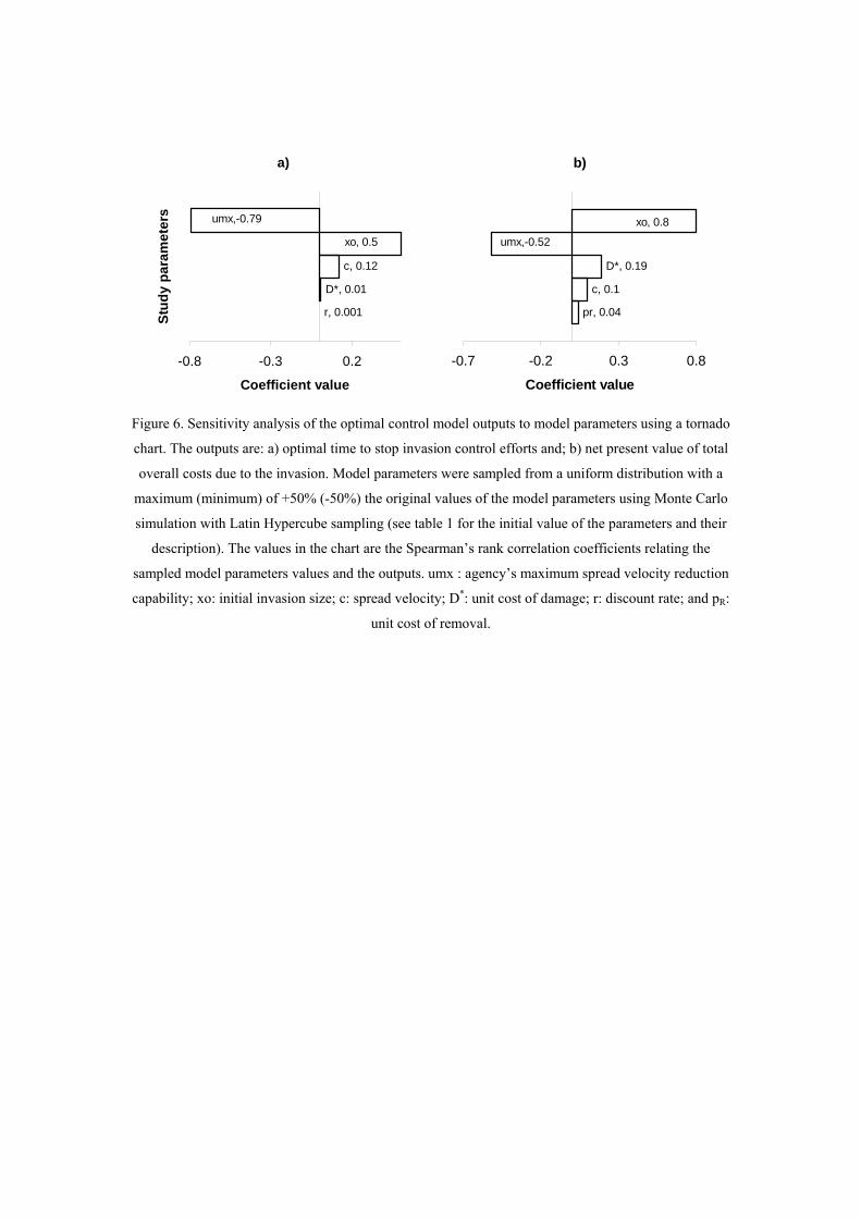
Sensitivity analysis

The sensitivity analysis confirmed the findings described above: the switching point

occurred closer to the beginning of the time horizon for high umax and closer to the end

of the time horizon for higher initial invasion sizes and spread velocities (Figure 6a);

and the total overall costs increased for higher initial invasion sizes, damage unit cost

and velocity of the invader and were reduced for high umax (Figure 6b).

Discussion

We have presented a simple, yet general, bioeconomic model to identify the switching

points for the management of a spreading invasion using barrier zones. In previous

work on this problem the Euler equation was employed (Sharov, 2004, Sharov and

Liebhold, 1998). We have used optimal control theory instead, which has the

advantage of considering explicitly the relationship between the control variable and

the state of the system (Chiang, 1992). In order to solve the optimal control problem,

we needed to establish the relationships between total removal costs, size of invasion

and total damage costs. Several empirical forms relating control and damage exist

(Lichtenberg and Zilberman, 1986). We chose those forms that provided a realistic

description of the system whilst being as simple as possible. We assumed a linear

relationship between the aimed spread velocity reduction and total costs of removal

and between the aimed spread velocity reduction and the reduction of spread velocity.

We assumed also a linear relationship between invasion size and total damage costs.

The choice of relationships influences the type of solution obtained. In our case, we

obtained a normal bang-bang solution (an example of a bang-bang solution in the

control of the spreading of plant diseases is found in Forster and Gilligan, 2007). This

indicates that it is optimum to spend either all resources on control or no resources at

all. We identified the switching point between maximum control and zero control, i.e.

the point at which any sort of control campaigns should end. In addition, since the

state variable (invasion size) was constrained, we identified two other points in time at

which control efforts should also cease: the time of eradication and the time at which

all the susceptible range is occupied. These points in time, together with the starting

and final points of the time horizon, shape the optimal control policy. Knowing the

critical switching points, we developed policy plots that can be used as preliminary

decision making tools in order to gauge the optimal policy given the ecological and

economic parameters of the invader and the ecosystem.

In the case of the potential Colorado potato beetle invasion in the UK, the optimal

policy for different combinations of model parameters confirmed previous findings in

the literature: Eradication was optimal for low initial sizes of invasion (Sharov, 2004)

and when there was a high agency’s maximum spread velocity reduction capability

(umax) (Figure 2). High umax also led to lower total overall costs of invasion (Figure 4a)

(Cacho et al., 2008; Hall and Hastings, 2007; Taylor, 2004). Eradication was also

preferred for low velocity of spread of the invader (Cacho, et al., 2008) provided the

ratio of unit cost of damage and removal per unit of area was not very low (Figure 3)

(Forster and Gilligan, 2007). Very low unit cost ratios made acceptance of the

invasion without attempt to control it the optimal policy (independently of the spread

velocity of the invader, Figure 3). Surprisingly, eradication was not always the

optimum policy even with sufficient outlays to carry it out (Figure 3). For the

majority of parameter combinations a policy switch happened within the time horizon,

showing how, even if eradication was not feasible, slowing down the spread until a

certain point in time was optimal (Sharov and Liebhold, 1998).

We assumed in the model that the government agency was fully aware of the initial

size of invasion upon discovery and of the effectiveness of the control measures over

the invasion size. Whereas this deterministic approach allows us to clearly identify the

trade-offs between parameters, the model would improve if these parameters were

depicted by uncertainty distributions and the problem solved using stochastic

optimization (Olson and Roy, 2005). The introduction of stochasticity is left,

tantalisingly, for future research. Population dynamics and dispersal processes are

also affected by stochasticity and Allee effects (Dennis, 2002), especially at low

population densities. We considered our approach reasonable since we focused on

already established and spreading organisms.

R-D models tend to underestimate the spread of organisms performing long distance

dispersal events (LDDE) (Andow et al., 1990). Since CPB can perform LDDE

assisted by weather events, R-D models might underestimate its dispersal in the UK.

Alternative spread models that account for LDDE could be incorporated in the

analytical model at the cost of increasing the complexity of the analytical analysis

(e.g. stratified diffusion models (Shigesada et al., 1995) and integro-difference models

(Kot et al., 1996)). This approach was regarded as beyond the scope of this study.

The assumption of constant umax presented the advantages of analytical tractability

and ease of interpretation (i.e. if the agency can maintain umax > c (spread velocity),

the invasion size will be reduced). A constant umax implies increasing (decreasing)

total costs of removal with increasing (decreasing) invasion size. In reality, the agency

will increase control efforts if the management measures are perceived as effective,

i.e. if a reduction of the invasion is achieved. In the same way, if initial control efforts

appear to be ineffective, they start to be gradually decreased.

The introduction of further non-linearities in the model could be considered. For

instance, Burnett et al., (2007) assumed increasing unit costs of removal with

decreasing sizes of invasion due to greater searching efforts. We judged that in our

case, the increase in the costs of trapping efforts for small population densities will

not be relevant enough as to justify making the unit cost of removal dependent on the

size of the invasion. In contrast, this is reasonable in their case, since the accessibility

to certain areas of the archipelago of Hawaii played an influential role on the

searching costs. In another instance, Sharov and Liebhold (1998) assumed that a

convex function would better explain the relationship between invasion size and total

costs of removal, by reflecting that big invasions would require the use of less

effective and hence marginally more costly control measures. In our case, we argue

that the invasion by CPB is not likely to exhaust the control resources of the plant

protection agency and hence the assumption of constant unit costs of removal would

be adequate.

Further improvements could be brought about by relaxing the assumption of an

homogeneous landscape. This could be achieved by adopting a spatially explicit

simulation approach. In this case, more flexible spread models like metapopulation

models (e.g. see an applications to bioeconomics by Brown and Roughgarden,

(1997)), cellular automata or individual based models (e.g. Breukers et al., 2006)

could be considered.

In this paper, a bioeconomic model to estimate the optimal policy and switching point

of invasion management campaigns was presented. This model represents a useful

tool for preliminary exploration of the optimal policy given a set of biological and

economic parameters. The integration of the dispersal patterns of the invader in the

bioeconomic modelling of IAS invasions is strongly recommended, as demonstrated

by this model. This integration will help us to estimate more precisely the time

periods during which we should apply the brake to IAS invasions, which can bring

about a greater measure of efficiency of control over these invasions.

Acknowledgements

We thank Christos Gavriel for his insights on optimal control theory. The research

was funded by a grant of the UK Department of Environment Food and Rural Affairs

(NB 53 9005) and the Rural Economy and Land Use Program (RES-229-25-0005).

References

Andow, D. A., Kareiva, P., Levin, S. A. and Okubo, A. ‘Spread of invading

organisms’, Landscape Ecology, Vol. 4, (1990) pp. 177-188.

Baker, R. H. A., Cannon, R. J. C., and Walters, K. F. A. ‘An assessment of the risks

posed by selected non-indigenous pests to UK crops under climate change’,

Aspects of Applied Biology, Vol. 45, (1996) pp. 323-330.

Bartlett, P. W. ‘Interception and eradication of Colorado beetle in England and Wales,

1958-1977’, Bulletin, Organisation Europeenne et Mediterranneenne pour la

Protection des Plantes, Vol. 10, (1980) pp. 481-489.

Breukers, A., Kettenis, D. L., Mourits, M., Van Der Werf, W. and Lansink, A. O.

‘Individual-based models in the analysis of disease transmission in plant

production chains: An application to potato brown rot’, Agricultural Systems,

Vol. 90, (2006) pp. 112-131.

Brown, G., and J. Roughgarden. ‘A metapopulation model with private property and a

common pool’, Ecological Economics, Vol. 22, (1997) pp. 65-71.

Burnett, K., B. Kaiser, and J. Roumasset. ‘Economic lessons from control efforts for

an invasive species: Miconia calvescens in Hawaii’, Journal of Forest

Economics, Vol. 13, (2007) pp. 151-167.

Burnett, K. M., D'evelyn, S., Kaiser, B. A., Nantamanasikarn, P. and Roumasset, J. A.

‘Beyond the lamppost: Optimal prevention and control of the Brown Tree

Snake in Hawaii’, Ecological Economics, Vol. 67, (2008) pp. 66-74.

Cacho, O. J., Wise, R. M., Hester, S. M. and Sinden, J. A. ‘Bioeconomic modeling for

control of weeds in natural environments’, Ecological Economics, Vol. 65,

(2008) pp. 559-568.

Chiang, A. C. Elements of Dynamic Optimization (New York: Mc Graw Hill, 1992).

Clark, C. W. Mathematical Bioeconomics: The Optimal Management Of Renewable

Resources (New York: J. Wiley, 1990).

DEFRA. The June Agricultural Survey, Department of Environment Food and Rural

Affairs. Farming Statistics Team (available at

http://www.defra.gov.uk/esg/work_htm/publications/cs/farmstats_web/default.

htm; last accessed February 2009; 2005)

Dennis, B. ‘Allee effects in stochastic populations’, Oikos, Vol. 96, (2002) pp. 389-

401.

Eiswerth, M. E., and G. C. Van Kooten. ‘The economics of invasive species

management: uncertainty, economics, and the spread of an invasive plant

species’, American Journal Of Agricultural Economics, Vol. 84, (2002) pp.

1317-1322.

EPPO. A2 List Of Pests Recommended For Regulation As Quarantine Pests,

European and Mediterranean Plant Protection Organisation, (available at

http://www.eppo.org/QUARANTINE/listA2.htm; last accessed February

2009; 2009).

Finnoff, D., Shogren, J. F., Leung, B. and Lodge, D. ‘Take a risk: Preferring

prevention over control of biological invaders’, Ecological Economics, Vol.

62, (2007) pp. 216-222.

Fisher, R. A. ‘The wave of advance of advantageous genes’, Annals of Eugenics, Vol.

7, (1937) pp. 355-369.

Follett, P. A., W. W. Cantelo, and G. K. Roderick. ‘Local dispersal of overwintered

Colorado potato beetle (Chrysomelidae: Coleoptera) determined by mark and

recapture.’, Environmental Entomology, Vol. 25, (1996) pp. 1304-1311.

Forster, G. A., and C. A. Gilligan. ‘Optimizing the control of disease infestations at

the landscape scale’, Proceedings of the National Academy of Sciences of the

United States of America, Vol. 104, (2007) pp. 4984-4989.

Hall, R. J., and A. Hastings. ‘Minimizing invader impacts: Striking the right balance

between removal and restoration’, Journal of Theoretical Biology, Vol. 249,

(2007) pp. 437-444.

Heikkila, J., and J. Peltola. ‘Analysis of the Colorado potato beetle protection system

in Finland’, Agricultural Economics, Vol. 31, (2004) pp. 343-352.

Higgins, S. I., and D. M. Richardson. ‘A review of models of alien plant spread’,

Ecological Modelling, Vol. 87, (1996) pp. 249-265.

Horan, R. D., Perrings, C., Lupi, F. and Bulte, E. H. ‘The economics of invasive

species management: biological pollution prevention strategies under

ignorance: the case of invasive species’, American Journal Of Agricultural

Economics, Vol. 84, (2002) pp. 1303.

Kim, C. S., Lubowski, R. N., Lewandrowski, J. and Eiswerth, M. E. ‘Prevention or

control: optimal government policies for invasive species management’,

Agricultural and Resource Economics Review, Vol. 35, (2006) pp. 29-40.

Kot, M., M. A. Lewis, and P. van den Driessche. ‘Dispersal data and the spread of

invading organisms’, Ecology, Vol. 77, (1996) pp. 2027-2042.

Leung, B., Lodge, D. M., Finnoff, D., Shogren, J. F., Lewis, M. A. and Lamberti, G.

‘An ounce of prevention or a pound of cure: bioeconomic risk analysis of

invasive species’, Proceedings of the Royal Society B: Biological Sciences,

Vol. 269, (2002) pp. 2407-2413.

Lewis, F. L., and V. L. Syrmos. Optimal Control (New York, Chichester: J. Wiley,

1995).

Lichtenberg, E., and D. Zilberman. ‘The Econometrics of Damage Control - Why

Specification Matters’, American Journal of Agricultural Economics, Vol. 68,

(1986) pp. 261-273.

Mack, R. N., Simberloff, D., Lonsdale, W. M., Evans, H., Clout, M. and Bazzaz, F. A.

‘Biotic invasions: Causes, epidemiology, global consequences, and control’,

Ecological Applications, Vol. 10, (2000) pp. 689-710.

Mumford, J. D., Temple, M., Quinlan, M. M., Gladders, P., Blood-Smyth, J.,

Mourato, S., Makuch, Z. and Crabb, J. Economic Evaluation Of MAFF's Plant

Health Programme, Report to Ministry of Agriculture, Fisheries and Food

(London, United Kingdom, 2000).

Odom, D. I. S., Cacho, O. J., Sinden, J. A. and Griffith, G. R. ‘Policies for the

management of weeds in natural ecosystems: the case of scotch broom

(Cytisus scoparius, L.) in an Australian national park’, Ecological Economics,

Vol. 44, (2003) pp. 119-135.

Olson, L. J., and S. Roy. ‘The economics of controlling a stochastic biological

invasion’, American Journal Of Agricultural Economics, Vol. 84, (2002) pp.

1311-1316.

Olson, L. J., and S. Roy. ‘On prevention and control of an uncertain biological

invasion’, Review of Agricultural Economics, Vol. 27, (2005) pp. 491-497.

Parker, I. I. M. ‘Impact: toward a framework for understanding the ecological effects

of invaders’, Biological Invasions, Vol. 1, (1999) pp. 3-19.

Sharov, A. A. ‘Bioeconomics of managing the spread of exotic pest species with

barrier zones’, Risk Analysis, Vol. 24, (2004) pp. 879-892.

Sharov, A. A., and A. M. Liebhold. ‘Bioeconomics of managing the spread of exotic

pest species with barrier zones’, Ecological Applications, Vol. 8, (1998) pp.

833-845.

Shigesada, N., K. Kawasaki, and Y. Takeda. ‘Modeling stratified diffusion in

biological invasions’, The American Naturalist, Vol. 146, (1995) pp. 229-251.

Skellman, J. G. ‘Random dispersal in theoretical populations’, Biometrika, Vol. 38,

(1951) pp. 196-218.

Taylor, C. M. ‘Finding optimal control strategies for invasive species: a density-

structured model for Spartina alterniflora’, Journal of Applied Ecology, Vol.

41, (2004) pp. 1049-1057.

Waage, J. K., Fraser, R. W., Mumford, J. D., Cook, D. C. and Wilby, A. A New

Agenda for Biosecurity: A Report for the Department for Food, Environment

And Rural Affairs, (London, United Kingdom: Imperial College London,

2005)

Wiktelius, S. ‘Wind dispersal in insects’, Grana, Vol. 20, (1981) pp. 205-207.

Yasar, B., and M. A. Gungor. ‘Determination of life table and biology of Colorado

potato beetle, Leptinotarsa decemlineata Say (Coleoptera : Chrysomelidae),

feeding on five different potato varieties in Turkey’, Applied Entomology and

Zoology, Vol. 40, (2005) pp. 589-596.

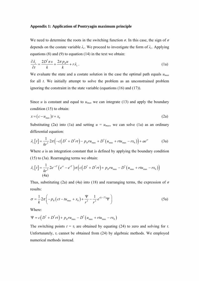
Appendix 1: Application of Pontryagin maximum principle

We need to determine the roots in the switching function σ. In this case, the sign of σ

depends on the costate variable λc. We proceed to investigate the form of λc. Applying

equations (8) and (9) to equation (14) in the text we obtain: * 22c R

cp uD x r

t k kλ ππ λ∂

= + +∂

. (1a)

We evaluate the state and a costate solution in the case the optimal path equals umax

for all t. We initially attempt to solve the problem as an unconstrained problem

ignoring the constraint in the state variable (equations (16) and (17)).

Since u is constant and equal to umax we can integrate (13) and apply the boundary

condition (15) to obtain:

( )max 0x c u t x= − + (2a)

Substituting (2a) into (1a) and setting u = umax, we can solve (1a) as an ordinary

differential equation:

[ ] ( ) (( )* * *max max max 02

1 2 rtc Rt c D D rt p ru D u rtu rx ae

krλ π= − + − + + − +) (3a)

Where a is an integration constant that is defined by applying the boundary condition

(15) to (3a). Rearranging terms we obtain:

[ ] ( ) ( ) ( )( )* * *max max max 02

1 2 rT rt rTc Rt e e e c D D rt p ru D u rtu rx

krλ π−= − + + − + −

(4a)

Thus, substituting (2a) and (4a) into (18) and rearranging terms, the expression of σ

results:

( ) ( )max 0 2 2

1 12 r t TRp ct tu x e

k r rσ π −Ψ⎛ ⎞= − − + + −⎜ ⎟

⎝ ⎠Ψ (5a)

Where:

( ) ( )* * *max max max 0Rc D D rt p ru D u rtu rxΨ = + + − + −

The switching points t = τi are obtained by equating (24) to zero and solving for t.

Unfortunately, τi cannot be obtained from (24) by algebraic methods. We employed

numerical methods instead.

The switching point τ corresponds to the solution of the unconstrained problem.

Taking into account the constraints of x in equations (16) and (17) implies that if τ is

greater than the time at which x = 0 (eradication occurs at t = terad) or x = xmax (total

invasion occurs at t = txmax) (we obtain terad and txmax by solving equation (2a) setting x

= 0 and x = xmax respectively), that solution occurs outside the permissible region.

Then the constraint of the state variable (either equation (16) or (17)) becomes

binding and by complementary slackness:

( ) 0u c− =

Since, by definition, c = 0 when x = 0 or x = xmax, u has to be zero as well.

Tables and figures

Table 1. Parameters of the model.

Symbol Description Value Source x0 Radius of initial size of invasion

(km) 20 Assumed

umax Agency’s maximum spread velocity reduction capability (km/year) 10 Assumed

pR Unit cost of removal (£/km2) 119.21 Estimated (Bartlett, 1980) D Diffusivity (km2/year) 60 (Waage et al., 2005) ε Intrinsic growth rate 0.04 Estimated (Yasar and Gungor, 2005) c Asymptotic velocity (km/year) 3.10 Estimated using Equation (2) Ch Historical spread Europe (km/year) 50 (Follett, et al., 1996) B Budget for control (£1000/year) 150 Assumed D* Unit cost of damage (£/km2) 50.29 (Waage et al., 2005) r Discount rate 0.06 Assumed xmaxA Maximum radius, circular invasion,

current climate (km) 159.07 Estimated (Baker et al., 1996).

xmaxB Maximum radius, semicircular invasion, current climate (km) 224.97 Estimated (Baker et al., 1996).

xmaxC Maximum radius, circular invasion, climate change (km) 226.17 Estimated (Baker et al., 1996).

xmaxD Maximum radius, semicircular invasion, climate change (km) 319.85 Estimated (Baker et al., 1996).

T Time horizon 20 Assumed Apotato Area of potato grown in England

and Wales (1000 ha) 142 Average from 2004 to 2008 (DEFRA, 2007).

Table 2. Effect of climate change, introduction point and spread velocity on Colorado potato beetle

optimal control policy in the UK. Eight scenarios are considered according to the climate projection:

current climate and climate change; the establishment point: centre of the susceptible range (centre)

and near the coast (coast); and the annual dispersal velocity of the invasion: predicted from the

reaction-diffusion model (c = 3.1 km/year); and assumed from historical spread rates in Europe (c = 50

km/year). The net prevent value (NVP) of costs reported are: R(x,u), total costs of removal; D(x) total

damage costs caused by the remaining invasion; total of overall costs (Total costs); switching time

from management to acceptance and the type of switch: τ, optimal time to stop control efforts; terad,

time at which eradication occurs; txmax time at which all the susceptible range is invaded; and the type

of optimal control policy (policy). Costs values are expressed in £ millions and switching time in years.

The rest of parameters of the model present the values in Table 1.

Climate Current climate scenario Climate change scenario c 3.1 50 3.1 50 Introduction centre coast centre coast centre coast centre coast R(x,u) 0.134 0.067 1.090 0.545 0.134 0.067 1.090 1.519 D(x) 0.031 0.015 40.095 20.047 0.031 0.015 74.625 64.610 Total costs 0.164 0.082 41.185 20.592 0.164 0.082 75.716 66.130 Switch time 3 3 2 2 3 3 2 4 Switch type terad terad txmax τ terad terad τ τ

§

Figure 1. Illustrative maps of the model predictions for the invasion by CPB in the UK after potential

establishment in the centre of the susceptible range and near the east coast. a) Natural spread without

control: the invasion expands its range continuously. b) Optimal control: the range of the invader is

reduced due to a moving barrier zone. Eradication occurs at the 8th year after discovery. The parameters

used by the model are those of Table 1.

0 80 160 240 32040Kilometers

a) Uncontrolled spreadIntroduction at the centre: xo = 20kmIntroduction near the coast: xo = 3km

Legend

Initial size of invasion (xo)

Spread after: a) 5; b) 1 year

Spread after: a) 10; b) 3 years

Spread after: a) 15; b) 5 years

Spread after: a) 20; b) 7 years

b) Optimal controlIntroduction at the centre: xo = 50kmIntroduction near the coast: xo = 50km

Figure 2. Policy plot of the optimal policy option for different radius of initial sizes of invasion (x0) and

agency’s maximum spread velocity reduction capability (umax) for the case of invasion by Colorado

potato beetle in the UK. Below (above) the dashed line: umax < CPB spread velocity (umax > CPB spread

velocity). The arrows indicate the progression of the size of the invasion under the optimal path. The

rest of the values were kept fixed at the values in Table 1.

1 15 30 45 60 75 90 105 120 135 1500.5

1.5

2.5

3.5

4.5

5.5

6.5

7.5

8.5

10

xo (km)

umax

(km

/yea

r)

Maximum control until eradication

Maximum control and then switch to acceptance

Maximum control until total invasion

0.02 0.11 0.23 0.42 0.78 1.69 8.021

3

5

7

9

11

13

15

17

19

cost ratio (D*/pr)

spre

ad v

eloc

ity (

km/y

ear)

Maximum control until eradication

Maximum control and then switch to acceptance

Maximum control until total invasionAcceptance without control

Figure 3. Policy plot of the optimal policy option depending on the unit cost ratio: unit cost of damage

(D*)/ unit cost of removal (pR) and the asymptotic spread velocity of the invader (c). The rest of the

parameters present the values in Table 1.

0123456789

0 1 2 3 4 5 6 7 8 9 10

umax (km/year)

NPV

tota

l cos

ts (£

mill

ions

)

D*/pr = 0.141D*/pr =0.422 D*/pr = 8.015

0

0.1

0.2

0.3

0.4

0.5

0.6

0.7

0.8

0 2 4 6 8 10

umax (km/year)

NPV

con

trol

cos

ts (£

mill

ion)

D*/pr = 0.141D*/pr = 0.422D*/pr = 8.015

b)

Figure 4. Net present value (NPV) of the total overall costs due to the invasion (a) and NPV of the total

costs of removal (b) for different agency’s maximum spread velocity reduction capability (umax). Three

levels of unit cost ratios (unit cost of damage, D*/ unit cost of removal, pR) were considered.

010203040506070

2 6 10 14 18

Spread velocity (km/year)

NPV

tota

l cos

ts (£

mill

ions

)xo = 20kmxo = 50kmxo = 80km

a)

0

2

4

6

8

10

12

2 6 10 14 18

Spread velocity (km/year)

NPV

con

trol

cos

ts (£

mill

ions

)

xo = 20kmxo = 50kmxo = 80km

b)

Figure 5. Net present value (NPV) of the total overall costs due to the invasion (a) and NPV of

the total costs of removal for different invader spread velocity. Three levels of initial size of invasion

(xo) were considered.

a)

r, 0.001

D*, 0.01

c, 0.12

xo, 0.5

umx,-0.79

-0.8 -0.3 0.2

Stud

y pa

ram

eter

s

Coefficient value

b)

pr, 0.04

c, 0.1

D*, 0.19

umx,-0.52

xo, 0.8

-0.7 -0.2 0.3 0.8

Coefficient value

Figure 6. Sensitivity analysis of the optimal control model outputs to model parameters using a tornado

chart. The outputs are: a) optimal time to stop invasion control efforts and; b) net present value of total

overall costs due to the invasion. Model parameters were sampled from a uniform distribution with a

maximum (minimum) of +50% (-50%) the original values of the model parameters using Monte Carlo

simulation with Latin Hypercube sampling (see table 1 for the initial value of the parameters and their

description). The values in the chart are the Spearman’s rank correlation coefficients relating the

sampled model parameters values and the outputs. umx : agency’s maximum spread velocity reduction

capability; xo: initial invasion size; c: spread velocity; D*: unit cost of damage; r: discount rate; and pR:

unit cost of removal.