The 30 Year Horizon - Axiomaxiom-developer.org/axiom-website/bookvol8.1.pdf · The 30 Year Horizon...
318
The 30 Year Horizon Manuel Bronstein William Burge T imothy Daly James Davenport Michael Dewar Martin Dunstan Albrecht F ortenbacher P atrizia Gianni Johannes Grabmeier Jocelyn Guidry Richard Jenks Larry Lambe Michael Monagan Scott Morrison William Sit Jonathan Steinbach Robert Sutor Barry Trager Stephen W att Jim Wen Clifton W illiamson Volume 8.1: Axiom Gallery April 15, 2018 27a6c3636e8a29e74cd7f58e4e93c30a0e05334e
Transcript of The 30 Year Horizon - Axiomaxiom-developer.org/axiom-website/bookvol8.1.pdf · The 30 Year Horizon...

The 30 Year Horizon
Manuel Bronstein William Burge T imothy DalyJames Davenport Michael Dewar Martin DunstanAlbrecht Fortenbacher Patrizia Gianni Johannes GrabmeierJocelyn Guidry Richard Jenks Larry LambeMichael Monagan Scott Morrison William SitJonathan Steinbach Robert Sutor Barry TragerStephen Watt Jim Wen Clifton Williamson
Volume 8.1: Axiom Gallery
April 15, 2018
27a6c3636e8a29e74cd7f58e4e93c30a0e05334e

i
Portions Copyright (c) 2005 Timothy Daly
The Blue Bayou image Copyright (c) 2004 Jocelyn Guidry
Portions Copyright (c) 2004 Martin Dunstan
Portions Copyright (c) 2007 Alfredo Portes
Portions Copyright (c) 2007 Arthur Ralfs
Portions Copyright (c) 2005 Timothy Daly
Portions Copyright (c) 1991-2002,
The Numerical ALgorithms Group Ltd.
All rights reserved.
This book and the Axiom software is licensed as follows:
Redistribution and use in source and binary forms, with or
without modification, are permitted provided that the following
conditions are
met:
- Redistributions of source code must retain the above
copyright notice, this list of conditions and the
following disclaimer.
- Redistributions in binary form must reproduce the above
copyright notice, this list of conditions and the
following disclaimer in the documentation and/or other
materials provided with the distribution.
- Neither the name of The Numerical ALgorithms Group Ltd.
nor the names of its contributors may be used to endorse
or promote products derived from this software without
specific prior written permission.
THIS SOFTWARE IS PROVIDED BY THE COPYRIGHT HOLDERS AND
CONTRIBUTORS "AS IS" AND ANY EXPRESS OR IMPLIED WARRANTIES,
INCLUDING, BUT NOT LIMITED TO, THE IMPLIED WARRANTIES OF
MERCHANTABILITY AND FITNESS FOR A PARTICULAR PURPOSE ARE
DISCLAIMED. IN NO EVENT SHALL THE COPYRIGHT OWNER OR
CONTRIBUTORS BE LIABLE FOR ANY DIRECT, INDIRECT, INCIDENTAL,
SPECIAL, EXEMPLARY, OR CONSEQUENTIAL DAMAGES (INCLUDING,
BUT NOT LIMITED TO, PROCUREMENT OF SUBSTITUTE GOODS OR
SERVICES; LOSS OF USE, DATA, OR PROFITS; OR BUSINESS
INTERRUPTION) HOWEVER CAUSED AND ON ANY THEORY OF LIABILITY,
WHETHER IN CONTRACT, STRICT LIABILITY, OR TORT (INCLUDING
NEGLIGENCE OR OTHERWISE) ARISING IN ANY WAY OUT OF THE USE
OF THIS SOFTWARE, EVEN IF ADVISED OF THE POSSIBILITY OF
SUCH DAMAGE.

ii
Inclusion of names in the list of credits is based on historical information and is as accurateas possible. Inclusion of names does not in any way imply an endorsement but representshistorical influence on Axiom development.

iii
Michael Albaugh Cyril Alberga Roy AdlerChristian Aistleitner Richard Anderson George AndrewsJerry Archibald S.J. Atkins Jeremy AvigadHenry Baker Martin Baker Stephen BalzacYurij Baransky David R. Barton Thomas BaruchelGerald Baumgartner Gilbert Baumslag Michael BeckerNelson H. F. Beebe Jay Belanger David BindelFred Blair Vladimir Bondarenko Mark BotchRaoul Bourquin Alexandre Bouyer Karen BramanWolfgang Brehm Peter A. Broadbery Martin BrockManuel Bronstein Christopher Brown Stephen BuchwaldFlorian Bundschuh Luanne Burns William BurgeRalph Byers Quentin Carpent Pierre CasteranRobert Cavines Bruce Char Ondrej CertikTzu-Yi Chen Bobby Cheng Cheekai ChinDavid V. Chudnovsky Gregory V. Chudnovsky Mark ClementsJames Cloos Jia Zhao Cong Josh CohenChristophe Conil Don Coppersmith George CorlissRobert Corless Gary Cornell Meino CramerKarl Crary Jeremy Du Croz David CyganskiNathaniel Daly Timothy Daly Sr. Timothy Daly Jr.James H. Davenport David Day James DemmelDidier Deshommes Michael Dewar Inderjit DhillonJack Dongarra Jean Della Dora Gabriel Dos ReisClaire DiCrescendo Sam Dooley Nicolas James DoyeZlatko Drmac Lionel Ducos Iain DuffLee Duhem Martin Dunstan Brian DupeeDominique Duval Robert Edwards Hans-Dieter EhrichHeow Eide-Goodman Lars Erickson Mark FaheyRichard Fateman Bertfried Fauser Stuart FeldmanJohn Fletcher Brian Ford Albrecht FortenbacherGeorge Frances Constantine Frangos Timothy FreemanKorrinn Fu Marc Gaetano Rudiger GebauerVan de Geijn Kathy Gerber Patricia GianniGustavo Goertkin Samantha Goldrich Holger GollanTeresa Gomez-Diaz Laureano Gonzalez-Vega Stephen GortlerJohannes Grabmeier Matt Grayson Klaus Ebbe GrueJames Griesmer Vladimir Grinberg Oswald GschnitzerMing Gu Jocelyn Guidry Gaetan HacheSteve Hague Satoshi Hamaguchi Sven HammarlingMike Hansen Richard Hanson Richard HarkeBill Hart Vilya Harvey Martin HassnerArthur S. Hathaway Dan Hatton Waldek HebischKarl Hegbloom Ralf Hemmecke HendersonAntoine Hersen Nicholas J. Higham Hoon HongRoger House Gernot Hueber Pietro IglioAlejandro Jakubi Richard Jenks Bo KagstromWilliam Kahan Kyriakos Kalorkoti Kai KaminskiGrant Keady Wilfrid Kendall Tony KennedyDavid Kincaid Keshav Kini Ted Kosan

iv
Paul Kosinski Igor Kozachenko Fred KroghKlaus Kusche Bernhard Kutzler Tim LaheyLarry Lambe Kaj Laurson Charles LawsonGeorge L. Legendre Franz Lehner Frederic LehobeyMichel Levaud Howard Levy J. LewisRen-Cang Li Rudiger Loos Craig LucasMichael Lucks Richard Luczak Camm MaguireFrancois Maltey Osni Marques Alasdair McAndrewBob McElrath Michael McGettrick Edi MeierIan Meikle David Mentre Victor S. MillerGerard Milmeister Mohammed Mobarak H. Michael MoellerMichael Monagan Marc Moreno-Maza Scott MorrisonJoel Moses Mark Murray William NaylorPatrice Naudin C. Andrew Neff John NelderGodfrey Nolan Arthur Norman Jinzhong NiuMichael O’Connor Summat Oemrawsingh Kostas OikonomouHumberto Ortiz-Zuazaga Julian A. Padget Bill PageDavid Parnas Susan Pelzel Michel PetitotDidier Pinchon Ayal Pinkus Frederick H. PittsFrank Pfenning Jose Alfredo Portes E. Quintana-OrtiGregorio Quintana-Orti Beresford Parlett A. PetitetAndre Platzer Peter Poromaas Claude QuitteArthur C. Ralfs Norman Ramsey Anatoly RaportirenkoGuilherme Reis Huan Ren Albert D. RichMichael Richardson Jason Riedy Renaud RiobooJean Rivlin Nicolas Robidoux Simon RobinsonRaymond Rogers Michael Rothstein Martin RubeyJeff Rutter Philip Santas David SaundersAlfred Scheerhorn William Schelter Gerhard SchneiderMartin Schoenert Marshall Schor Frithjof SchulzeFritz Schwarz Steven Segletes V. SimaNick Simicich William Sit Elena SmirnovaJacob Nyffeler Smith Matthieu Sozeau Ken StanleyJonathan Steinbach Fabio Stumbo Christine SundaresanKlaus Sutner Robert Sutor Moss E. SweedlerEugene Surowitz Yong Kiam Tan Max TegmarkT. Doug Telford James Thatcher Laurent TheryBalbir Thomas Mike Thomas Dylan ThurstonFrancoise Tisseur Steve Toleque Raymond ToyBarry Trager Themos T. Tsikas Gregory VanuxemKresimir Veselic Christof Voemel Bernhard WallStephen Watt Andreas Weber Jaap WeelJuergen Weiss M. Weller Mark WegmanJames Wen Thorsten Werther Michael WesterR. Clint Whaley James T. Wheeler John M. WileyBerhard Will Clifton J. Williamson Stephen WilsonShmuel Winograd Robert Wisbauer Sandra WityakWaldemar Wiwianka Knut Wolf Yanyang XiaoLiu Xiaojun Clifford Yapp David YunQian Yun Vadim Zhytnikov Richard ZippelEvelyn Zoernack Bruno Zuercher Dan Zwillinger

Contents
1 General examples 1
1.1 Two dimensional functions . . . . . . . . . . . . . . . . . . . . . . . . . . . . . 1
1.1.1 A Simple Sine Function . . . . . . . . . . . . . . . . . . . . . . . . . . 2
1.1.2 A Simple Sine Function, Non-adaptive plot . . . . . . . . . . . . . . . 3
1.1.3 A Simple Sine Function, Drawn to Scale . . . . . . . . . . . . . . . . . 4
1.1.4 A Simple Sine Function, Polar Plot . . . . . . . . . . . . . . . . . . . . 5
1.1.5 A Simple Tangent Function, Clipping On . . . . . . . . . . . . . . . . 6
1.1.6 A Simple Tangent Function, Clipping On . . . . . . . . . . . . . . . . 7
1.1.7 Tangent and Sine . . . . . . . . . . . . . . . . . . . . . . . . . . . . . . 8
1.1.8 A 2D Sine Function in BiPolar Coordinates . . . . . . . . . . . . . . . 9
1.1.9 A 2D Sine Function in Elliptic Coordinates . . . . . . . . . . . . . . . 10
1.1.10 A 2D Sine Wave in Polar Coordinates . . . . . . . . . . . . . . . . . . 11
1.2 Two dimensional curves . . . . . . . . . . . . . . . . . . . . . . . . . . . . . . 11
1.2.1 A Line in Parabolic Coordinates . . . . . . . . . . . . . . . . . . . . . 12
1.2.2 Lissajous Curve . . . . . . . . . . . . . . . . . . . . . . . . . . . . . . . 13
1.2.3 A Parametric Curve . . . . . . . . . . . . . . . . . . . . . . . . . . . . 14
1.2.4 A Parametric Curve in Polar Coordinates . . . . . . . . . . . . . . . . 15
1.3 Three dimensional functions . . . . . . . . . . . . . . . . . . . . . . . . . . . . 15
1.3.1 A 3D Constant Function in Elliptic Coordinates . . . . . . . . . . . . 16
1.3.2 A 3D Constant Function in Oblate Spheroidal . . . . . . . . . . . . . 17
1.3.3 A 3D Constant in Polar Coordinates . . . . . . . . . . . . . . . . . . . 18
1.3.4 A 3D Constant in Prolate Spheroidal Coordinates . . . . . . . . . . . 19
1.3.5 A 3D Constant in Spherical Coordinates . . . . . . . . . . . . . . . . . 20
1.3.6 A 2-Equation Space Function . . . . . . . . . . . . . . . . . . . . . . . 21
1.4 Three dimensional curves . . . . . . . . . . . . . . . . . . . . . . . . . . . . . 21
v

vi CONTENTS
1.4.1 A Parametric Space Curve . . . . . . . . . . . . . . . . . . . . . . . . 22
1.4.2 A Tube around a Parametric Space Curve . . . . . . . . . . . . . . . . 23
1.4.3 A 2-Equation Cylindrical Curve . . . . . . . . . . . . . . . . . . . . . . 24
1.5 Three dimensional surfaces . . . . . . . . . . . . . . . . . . . . . . . . . . . . 24
1.5.1 A Icosahedron . . . . . . . . . . . . . . . . . . . . . . . . . . . . . . . 25
1.5.2 A 3D figure 8 immersion (Klein bagel) . . . . . . . . . . . . . . . . . . 27
1.5.3 A 2-Equation bipolarCylindrical Surface . . . . . . . . . . . . . . . . . 28
1.5.4 A 3-Equation Parametric Space Surface . . . . . . . . . . . . . . . . . 29
1.5.5 A 3D Vector of Points in Elliptic Cylindrical . . . . . . . . . . . . . . 30
1.5.6 A 3D Constant Function in BiPolar Coordinates . . . . . . . . . . . . 31
1.5.7 A Swept in Parabolic Coordinates . . . . . . . . . . . . . . . . . . . . 32
1.5.8 A Swept Cone in Parabolic Cylindrical Coordinates . . . . . . . . . . 33
1.5.9 A Truncated Cone in Toroidal Coordinates . . . . . . . . . . . . . . . 34
1.5.10 A Swept Surface in Paraboloidal Coordinates . . . . . . . . . . . . . . 35
2 Jenks Book images 37
2.0.11 The Complex Gamma Function . . . . . . . . . . . . . . . . . . . . . . 38
2.0.12 The Complex Arctangent Function . . . . . . . . . . . . . . . . . . . . 39
3 Hyperdoc examples 41
3.1 Two dimensional examples . . . . . . . . . . . . . . . . . . . . . . . . . . . . . 41
3.1.1 A function of one variable . . . . . . . . . . . . . . . . . . . . . . . . . 42
3.1.2 A Parametric function . . . . . . . . . . . . . . . . . . . . . . . . . . . 43
3.1.3 A Polynomial in 2 variables . . . . . . . . . . . . . . . . . . . . . . . . 44
3.2 Three dimensional examples . . . . . . . . . . . . . . . . . . . . . . . . . . . . 44
3.2.1 A function of two variables . . . . . . . . . . . . . . . . . . . . . . . . 45
3.2.2 A parametrically defined curve . . . . . . . . . . . . . . . . . . . . . . 46
3.2.3 A parametrically defined surface . . . . . . . . . . . . . . . . . . . . . 47
4 CRC Standard Curves and Surfaces 49
4.1 Standard Curves and Surfaces . . . . . . . . . . . . . . . . . . . . . . . . . . . 49
4.2 CRC graphs . . . . . . . . . . . . . . . . . . . . . . . . . . . . . . . . . . . . . 50
4.2.1 Functions with xn/m . . . . . . . . . . . . . . . . . . . . . . . . . . . . 50
4.2.2 Functions with xn and (a+ bx)m . . . . . . . . . . . . . . . . . . . . . 61

CONTENTS vii
4.2.3 Functions with a2 + x2 and xm . . . . . . . . . . . . . . . . . . . . . . 116
4.2.4 Functions with a2 − x2 and xm . . . . . . . . . . . . . . . . . . . . . . 130
4.2.5 Functions with a3 + x3 and xm . . . . . . . . . . . . . . . . . . . . . . 144
4.2.6 Functions with a3 − x3 and xm . . . . . . . . . . . . . . . . . . . . . . 155
4.2.7 Functions with a4 + x4 and xm . . . . . . . . . . . . . . . . . . . . . . 166
4.2.8 Functions with a4 − x4 and xm . . . . . . . . . . . . . . . . . . . . . . 177
4.2.9 Functions with (a+ bx)1/2 and xm . . . . . . . . . . . . . . . . . . . . 188
5 Pasta by Design 207
5.1 Acini Di Pepe . . . . . . . . . . . . . . . . . . . . . . . . . . . . . . . . . . . . 208
5.2 Agnolotti . . . . . . . . . . . . . . . . . . . . . . . . . . . . . . . . . . . . . . 209
5.3 Anellini . . . . . . . . . . . . . . . . . . . . . . . . . . . . . . . . . . . . . . . 210
5.4 Bucatini . . . . . . . . . . . . . . . . . . . . . . . . . . . . . . . . . . . . . . . 211
5.5 Buccoli . . . . . . . . . . . . . . . . . . . . . . . . . . . . . . . . . . . . . . . 212
5.6 Calamaretti . . . . . . . . . . . . . . . . . . . . . . . . . . . . . . . . . . . . . 213
5.7 Cannelloni . . . . . . . . . . . . . . . . . . . . . . . . . . . . . . . . . . . . . . 214
5.8 Cannolicchi Rigati . . . . . . . . . . . . . . . . . . . . . . . . . . . . . . . . . 215
5.9 Capellini . . . . . . . . . . . . . . . . . . . . . . . . . . . . . . . . . . . . . . . 216
5.10 Cappelletti . . . . . . . . . . . . . . . . . . . . . . . . . . . . . . . . . . . . . 217
5.11 Casarecce . . . . . . . . . . . . . . . . . . . . . . . . . . . . . . . . . . . . . . 218
5.12 Castellane . . . . . . . . . . . . . . . . . . . . . . . . . . . . . . . . . . . . . . 219
5.13 Cavatappi . . . . . . . . . . . . . . . . . . . . . . . . . . . . . . . . . . . . . . 220
5.14 Cavatelli . . . . . . . . . . . . . . . . . . . . . . . . . . . . . . . . . . . . . . . 221
5.15 Chifferi Rigati . . . . . . . . . . . . . . . . . . . . . . . . . . . . . . . . . . . . 222
5.16 Colonne Pompeii . . . . . . . . . . . . . . . . . . . . . . . . . . . . . . . . . . 223
5.17 Conchiglie Rigate . . . . . . . . . . . . . . . . . . . . . . . . . . . . . . . . . . 225
5.18 Conchigliette Lisce . . . . . . . . . . . . . . . . . . . . . . . . . . . . . . . . . 226
5.19 Conchiglioni Rigate . . . . . . . . . . . . . . . . . . . . . . . . . . . . . . . . . 227
5.20 Corallini Lisci . . . . . . . . . . . . . . . . . . . . . . . . . . . . . . . . . . . . 228
5.21 Creste Di Galli . . . . . . . . . . . . . . . . . . . . . . . . . . . . . . . . . . . 229
5.22 Couretti . . . . . . . . . . . . . . . . . . . . . . . . . . . . . . . . . . . . . . . 230
5.23 Ditali Rigati . . . . . . . . . . . . . . . . . . . . . . . . . . . . . . . . . . . . . 231
5.24 Fagottini . . . . . . . . . . . . . . . . . . . . . . . . . . . . . . . . . . . . . . . 232
5.25 Farfalle . . . . . . . . . . . . . . . . . . . . . . . . . . . . . . . . . . . . . . . 233

viii CONTENTS
5.26 Farfalline . . . . . . . . . . . . . . . . . . . . . . . . . . . . . . . . . . . . . . 235
5.27 Farfalloni . . . . . . . . . . . . . . . . . . . . . . . . . . . . . . . . . . . . . . 236
5.28 Festonati . . . . . . . . . . . . . . . . . . . . . . . . . . . . . . . . . . . . . . 237
5.29 Fettuccine . . . . . . . . . . . . . . . . . . . . . . . . . . . . . . . . . . . . . . 238
5.30 Fiocchi Rigati . . . . . . . . . . . . . . . . . . . . . . . . . . . . . . . . . . . . 239
5.31 Fisarmoniche . . . . . . . . . . . . . . . . . . . . . . . . . . . . . . . . . . . . 240
5.32 Funghini . . . . . . . . . . . . . . . . . . . . . . . . . . . . . . . . . . . . . . . 241
5.33 Fusilli . . . . . . . . . . . . . . . . . . . . . . . . . . . . . . . . . . . . . . . . 242
5.34 Fusilli al Ferretto . . . . . . . . . . . . . . . . . . . . . . . . . . . . . . . . . . 243
5.35 Fusilli Capri . . . . . . . . . . . . . . . . . . . . . . . . . . . . . . . . . . . . . 244
5.36 Fusilli Lunghi Bucati . . . . . . . . . . . . . . . . . . . . . . . . . . . . . . . . 245
5.37 Galletti . . . . . . . . . . . . . . . . . . . . . . . . . . . . . . . . . . . . . . . 247
5.38 Garganelli . . . . . . . . . . . . . . . . . . . . . . . . . . . . . . . . . . . . . . 248
5.39 Gemelli . . . . . . . . . . . . . . . . . . . . . . . . . . . . . . . . . . . . . . . 249
5.40 Gigli . . . . . . . . . . . . . . . . . . . . . . . . . . . . . . . . . . . . . . . . . 250
5.41 Giglio Ondulato . . . . . . . . . . . . . . . . . . . . . . . . . . . . . . . . . . . 251
5.42 Gnocchetti Sardi . . . . . . . . . . . . . . . . . . . . . . . . . . . . . . . . . . 252
5.43 Gnocchi . . . . . . . . . . . . . . . . . . . . . . . . . . . . . . . . . . . . . . . 253
5.44 Gramigna . . . . . . . . . . . . . . . . . . . . . . . . . . . . . . . . . . . . . . 254
5.45 Lancette . . . . . . . . . . . . . . . . . . . . . . . . . . . . . . . . . . . . . . . 255
5.46 Lasagna Larga Doppia Riccia . . . . . . . . . . . . . . . . . . . . . . . . . . . 256
5.47 Linguine . . . . . . . . . . . . . . . . . . . . . . . . . . . . . . . . . . . . . . . 257
5.48 Lumaconi Rigati . . . . . . . . . . . . . . . . . . . . . . . . . . . . . . . . . . 258
5.49 Maccheroni . . . . . . . . . . . . . . . . . . . . . . . . . . . . . . . . . . . . . 259
5.50 Maccheroni Alla Chitarra . . . . . . . . . . . . . . . . . . . . . . . . . . . . . 260
5.51 Mafaldine . . . . . . . . . . . . . . . . . . . . . . . . . . . . . . . . . . . . . . 261
5.52 Manicotti . . . . . . . . . . . . . . . . . . . . . . . . . . . . . . . . . . . . . . 262
5.53 Orecchiette . . . . . . . . . . . . . . . . . . . . . . . . . . . . . . . . . . . . . 263
5.54 Paccheri . . . . . . . . . . . . . . . . . . . . . . . . . . . . . . . . . . . . . . . 264
5.55 Pappardelle . . . . . . . . . . . . . . . . . . . . . . . . . . . . . . . . . . . . . 265
5.56 Penne Rigate . . . . . . . . . . . . . . . . . . . . . . . . . . . . . . . . . . . . 266
5.57 Pennoni Lisci . . . . . . . . . . . . . . . . . . . . . . . . . . . . . . . . . . . . 267
5.58 Pennoni Rigati . . . . . . . . . . . . . . . . . . . . . . . . . . . . . . . . . . . 268

CONTENTS ix
5.59 Puntalette . . . . . . . . . . . . . . . . . . . . . . . . . . . . . . . . . . . . . . 269
5.60 Quadrefiore . . . . . . . . . . . . . . . . . . . . . . . . . . . . . . . . . . . . . 270
5.61 Quadretti . . . . . . . . . . . . . . . . . . . . . . . . . . . . . . . . . . . . . . 271
5.62 Racchette . . . . . . . . . . . . . . . . . . . . . . . . . . . . . . . . . . . . . . 272
5.63 Radiatori . . . . . . . . . . . . . . . . . . . . . . . . . . . . . . . . . . . . . . 273
5.64 Ravioli Quadrati . . . . . . . . . . . . . . . . . . . . . . . . . . . . . . . . . . 274
5.65 Ravioli Tondi . . . . . . . . . . . . . . . . . . . . . . . . . . . . . . . . . . . . 275
5.66 Riccioli . . . . . . . . . . . . . . . . . . . . . . . . . . . . . . . . . . . . . . . 276
5.67 Riccioli al Cinque Sapori . . . . . . . . . . . . . . . . . . . . . . . . . . . . . . 277
5.68 Rigatoni . . . . . . . . . . . . . . . . . . . . . . . . . . . . . . . . . . . . . . . 278
5.69 Rombi . . . . . . . . . . . . . . . . . . . . . . . . . . . . . . . . . . . . . . . . 279
5.70 Rotelle . . . . . . . . . . . . . . . . . . . . . . . . . . . . . . . . . . . . . . . . 280
5.71 Saccottini . . . . . . . . . . . . . . . . . . . . . . . . . . . . . . . . . . . . . . 281
5.72 Sagnarelli . . . . . . . . . . . . . . . . . . . . . . . . . . . . . . . . . . . . . . 282
5.73 Sagne Incannulate . . . . . . . . . . . . . . . . . . . . . . . . . . . . . . . . . 283
5.74 Scialatielli . . . . . . . . . . . . . . . . . . . . . . . . . . . . . . . . . . . . . . 284
5.75 Spaccatelle . . . . . . . . . . . . . . . . . . . . . . . . . . . . . . . . . . . . . 285
5.76 Spaghetti . . . . . . . . . . . . . . . . . . . . . . . . . . . . . . . . . . . . . . 286
5.77 Spiralli . . . . . . . . . . . . . . . . . . . . . . . . . . . . . . . . . . . . . . . . 287
5.78 Stellette . . . . . . . . . . . . . . . . . . . . . . . . . . . . . . . . . . . . . . . 288
5.79 Stortini . . . . . . . . . . . . . . . . . . . . . . . . . . . . . . . . . . . . . . . 289
5.80 Strozzapreti . . . . . . . . . . . . . . . . . . . . . . . . . . . . . . . . . . . . . 290
5.81 Tagliatelle . . . . . . . . . . . . . . . . . . . . . . . . . . . . . . . . . . . . . . 291
5.82 Taglierini . . . . . . . . . . . . . . . . . . . . . . . . . . . . . . . . . . . . . . 292
5.83 Tagliolini . . . . . . . . . . . . . . . . . . . . . . . . . . . . . . . . . . . . . . 293
5.84 Torchietti . . . . . . . . . . . . . . . . . . . . . . . . . . . . . . . . . . . . . . 294
5.85 Tortellini . . . . . . . . . . . . . . . . . . . . . . . . . . . . . . . . . . . . . . 295
5.86 Tortiglioni . . . . . . . . . . . . . . . . . . . . . . . . . . . . . . . . . . . . . . 296
5.87 Trenne . . . . . . . . . . . . . . . . . . . . . . . . . . . . . . . . . . . . . . . . 297
5.88 Tripoline . . . . . . . . . . . . . . . . . . . . . . . . . . . . . . . . . . . . . . . 298
5.89 Trofie . . . . . . . . . . . . . . . . . . . . . . . . . . . . . . . . . . . . . . . . 299
5.90 Trottole . . . . . . . . . . . . . . . . . . . . . . . . . . . . . . . . . . . . . . . 300
5.91 Tubetti Rigati . . . . . . . . . . . . . . . . . . . . . . . . . . . . . . . . . . . . 301

x CONTENTS
5.92 Ziti . . . . . . . . . . . . . . . . . . . . . . . . . . . . . . . . . . . . . . . . . . 302
Bibliography 303
Index 305

CONTENTS xi
New Foreword
On October 1, 2001 Axiom was withdrawn from the market and ended life as a commer-cial product. On September 3, 2002 Axiom was released under the Modified BSD license,including this document. On August 27, 2003 Axiom was released as free and open sourcesoftware available for download from the Free Software Foundation’s website, Savannah.
Work on Axiom has had the generous support of the Center for Algorithms and InteractiveScientific Computation (CAISS) at City College of New York. Special thanks go to Dr.Gilbert Baumslag for his support of the long term goal.
The online version of this documentation is roughly 1000 pages. In order to make printedversions we’ve broken it up into three volumes. The first volume is tutorial in nature. Thesecond volume is for programmers. The third volume is reference material. We’ve also addeda fourth volume for developers. All of these changes represent an experiment in print-on-demand delivery of documentation. Time will tell whether the experiment succeeded.
Axiom has been in existence for over thirty years. It is estimated to contain about threehundred man-years of research and has, as of September 3, 2003, 143 people listed in thecredits. All of these people have contributed directly or indirectly to making Axiom available.Axiom is being passed to the next generation. I’m looking forward to future milestones.
With that in mind I’ve introduced the theme of the “30 year horizon”. We must inventthe tools that support the Computational Mathematician working 30 years from now. Howwill research be done when every bit of mathematical knowledge is online and instantlyavailable? What happens when we scale Axiom by a factor of 100, giving us 1.1 milliondomains? How can we integrate theory with code? How will we integrate theorems andproofs of the mathematics with space-time complexity proofs and running code? Whatvisualization tools are needed? How do we support the conceptual structures and semanticsof mathematics in effective ways? How do we support results from the sciences? How do weteach the next generation to be effective Computational Mathematicians?
The “30 year horizon” is much nearer than it appears.
Tim DalyCAISS, City College of New YorkNovember 10, 2003 ((iHy))

Chapter 1
General examples
These examples come from code that ships with Axiom in various input files.
1.1 Two dimensional functions
1

2 CHAPTER 1. GENERAL EXAMPLES
1.1.1 A Simple Sine Function
— equation123 —
draw(sin(11*x),x = 0..2*%pi)
———-

1.1. TWO DIMENSIONAL FUNCTIONS 3
1.1.2 A Simple Sine Function, Non-adaptive plot
— equation124 —
draw(sin(11*x),x = 0..2*%pi,adaptive == false,title == "Non-adaptive plot")
———-

4 CHAPTER 1. GENERAL EXAMPLES
1.1.3 A Simple Sine Function, Drawn to Scale
— equation125 —
draw(sin(11*x),x = 0..2*%pi,toScale == true,title == "Drawn to scale")
———-

1.1. TWO DIMENSIONAL FUNCTIONS 5
1.1.4 A Simple Sine Function, Polar Plot
— equation126 —
draw(sin(11*x),x = 0..2*%pi,coordinates == polar,title == "Polar plot")
———-

6 CHAPTER 1. GENERAL EXAMPLES
1.1.5 A Simple Tangent Function, Clipping On
— equation127 —
draw(tan x,x = -6..6,title == "Clipping on")
———-
1.1. TWO DIMENSIONAL FUNCTIONS 7
1.1.6 A Simple Tangent Function, Clipping On
— equation128 —
draw(tan x,x = -6..6,clip == false,title == "Clipping off")
———-
8 CHAPTER 1. GENERAL EXAMPLES
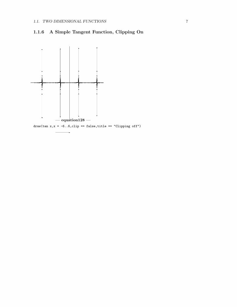
1.1.7 Tangent and Sine
— equation101 —
f(x:DFLOAT):DFLOAT == sin(tan(x))-tan(sin(x))
draw(f,0..6)
———-

1.1. TWO DIMENSIONAL FUNCTIONS 9
1.1.8 A 2D Sine Function in BiPolar Coordinates
— equation107 —
draw(sin(x),x=0.5..%pi,coordinates == bipolar(1$DFLOAT))
———-
10 CHAPTER 1. GENERAL EXAMPLES
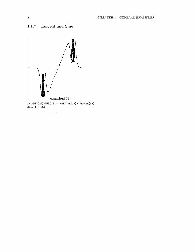
1.1.9 A 2D Sine Function in Elliptic Coordinates
— equation110 —
draw(sin(4*t/7),t=0..14*%pi,coordinates == elliptic(1$DFLOAT))
———-

1.2. TWO DIMENSIONAL CURVES 11
1.1.10 A 2D Sine Wave in Polar Coordinates
— equation118 —
draw(sin(4*t/7),t=0..14*%pi,coordinates == polar)
———-
1.2 Two dimensional curves

12 CHAPTER 1. GENERAL EXAMPLES
1.2.1 A Line in Parabolic Coordinates
— equation114 —
h1(t:DFLOAT):DFLOAT == t
h2(t:DFLOAT):DFLOAT == 2
draw(curve(h1,h2),-3..3,coordinates == parabolic)
———-

1.2. TWO DIMENSIONAL CURVES 13
1.2.2 Lissajous Curve
— equation102 —
i1(t:DFLOAT):DFLOAT == 9*sin(3*t/4)
i2(t:DFLOAT):DFLOAT == 8*sin(t)
draw(curve(i1,i2),-4*%pi..4*%pi,toScale == true, title == "Lissajous Curve")
———-
14 CHAPTER 1. GENERAL EXAMPLES
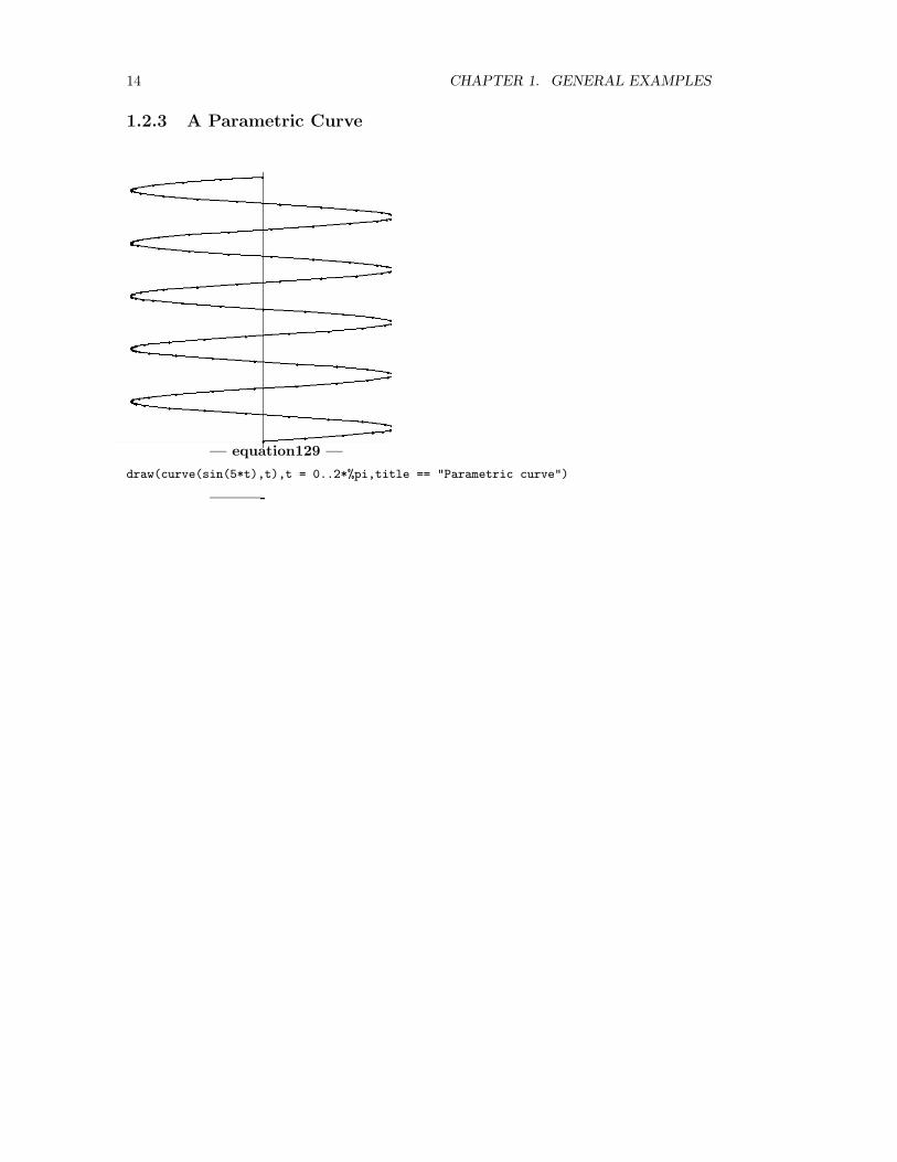
1.2.3 A Parametric Curve
— equation129 —
draw(curve(sin(5*t),t),t = 0..2*%pi,title == "Parametric curve")
———-

1.3. THREE DIMENSIONAL FUNCTIONS 15
1.2.4 A Parametric Curve in Polar Coordinates
— equation130 —
draw(curve(sin(5*t),t),t = 0..2*%pi,_
coordinates == polar,title == "Parametric polar curve")
———-
1.3 Three dimensional functions

16 CHAPTER 1. GENERAL EXAMPLES
1.3.1 A 3D Constant Function in Elliptic Coordinates
— equation111 —
m(u:DFLOAT,v:DFLOAT):DFLOAT == 1
draw(m,0..2*%pi,0..%pi,coordinates == elliptic(1$DFLOAT))
———-

1.3. THREE DIMENSIONAL FUNCTIONS 17
1.3.2 A 3D Constant Function in Oblate Spheroidal
— equation113 —
m(u:DFLOAT,v:DFLOAT):DFLOAT == 1
draw(m,-%pi/2..%pi/2,0..2*%pi,coordinates == oblateSpheroidal(1$DFLOAT))
———-

18 CHAPTER 1. GENERAL EXAMPLES
1.3.3 A 3D Constant in Polar Coordinates
— equation119 —
m(u:DFLOAT,v:DFLOAT):DFLOAT == 1
draw(m,0..2*%pi, 0..%pi,coordinates == polar)
———-
1.3. THREE DIMENSIONAL FUNCTIONS 19
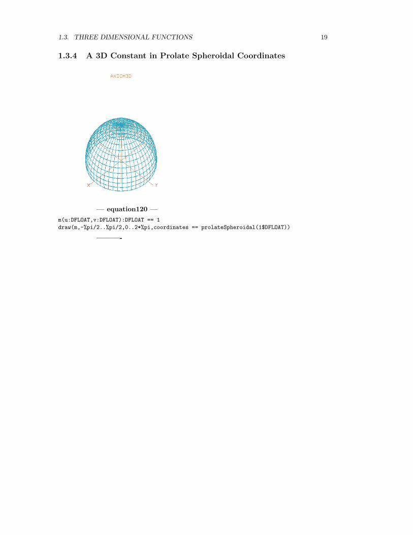
1.3.4 A 3D Constant in Prolate Spheroidal Coordinates
— equation120 —
m(u:DFLOAT,v:DFLOAT):DFLOAT == 1
draw(m,-%pi/2..%pi/2,0..2*%pi,coordinates == prolateSpheroidal(1$DFLOAT))
———-
20 CHAPTER 1. GENERAL EXAMPLES
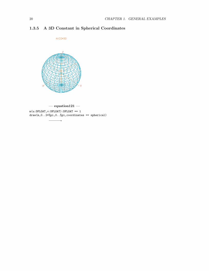
1.3.5 A 3D Constant in Spherical Coordinates
— equation121 —
m(u:DFLOAT,v:DFLOAT):DFLOAT == 1
draw(m,0..2*%pi,0..%pi,coordinates == spherical)
———-

1.4. THREE DIMENSIONAL CURVES 21
1.3.6 A 2-Equation Space Function
— equation104 —
f(x:DFLOAT,y:DFLOAT):DFLOAT == cos(x*y)
colorFxn(x:DFLOAT,y:DFLOAT):DFLOAT == 1/(x**2 + y**2 + 1)
draw(f,-3..3,-3..3, colorFunction == colorFxn,title=="2-Equation Space Curve")
———-
1.4 Three dimensional curves

22 CHAPTER 1. GENERAL EXAMPLES
1.4.1 A Parametric Space Curve
— equation131 —
draw(curve(sin(t)*cos(3*t/5),cos(t)*cos(3*t/5),cos(t)*sin(3*t/5)),_
t = 0..15*%pi,title == "Parametric curve")
———-

1.4. THREE DIMENSIONAL CURVES 23
1.4.2 A Tube around a Parametric Space Curve
— equation132 —
draw(curve(sin(t)*cos(3*t/5),cos(t)*cos(3*t/5),cos(t)*sin(3*t/5)),_
t = 0..15*%pi,tubeRadius == .15,title == "Tube around curve")
———-

24 CHAPTER 1. GENERAL EXAMPLES
1.4.3 A 2-Equation Cylindrical Curve
— equation109 —
j1(t:DFLOAT):DFLOAT == 4
j2(t:DFLOAT):DFLOAT == t
draw(curve(j1,j2,j2),-9..9,coordinates == cylindrical)
———-
1.5 Three dimensional surfaces

1.5. THREE DIMENSIONAL SURFACES 25
1.5.1 A Icosahedron
— Icosahedron —
)se exp add con InnerTrigonometricManipulations
exp(%i*2*%pi/5)
FG2F %
% -1
complexForm %
norm %
simplify %
s:=sqrt %
ph:=exp(%i*2*%pi/5)
A1:=complex(1,0)
A2:=A1*ph
A3:=A2*ph
A4:=A3*ph
A5:=A4*ph
ca1:=map(numeric , complexForm FG2F simplify A1)
ca2:=map(numeric , complexForm FG2F simplify A2)
ca3:=map(numeric ,complexForm FG2F simplify A3)
ca4:=map(numeric ,complexForm FG2F simplify A4)
ca5:=map(numeric ,complexForm FG2F simplify A5)
B1:=A1*exp(2*%i*%pi/10)
B2:=B1*ph
B3:=B2*ph
B4:=B3*ph
B5:=B4*ph
cb1:=map (numeric ,complexForm FG2F simplify B1)
cb2:=map (numeric ,complexForm FG2F simplify B2)
cb3:=map (numeric ,complexForm FG2F simplify B3)
cb4:=map (numeric ,complexForm FG2F simplify B4)
cb5:=map (numeric ,complexForm FG2F simplify B5)
u:=numeric sqrt(s*s-1)
p0:=point([0,0,u+1/2])@Point(SF)
p1:=point([real ca1,imag ca1,0.5])@Point(SF)

26 CHAPTER 1. GENERAL EXAMPLES
p2:=point([real ca2,imag ca2,0.5])@Point(SF)
p3:=point([real ca3,imag ca3,0.5])@Point(SF)
p4:=point([real ca4,imag ca4,0.5])@Point(SF)
p5:=point([real ca5,imag ca5,0.5])@Point(SF)
p6:=point([real cb1,imag cb1,-0.5])@Point(SF)
p7:=point([real cb2,imag cb2,-0.5])@Point(SF)
p8:=point([real cb3,imag cb3,-0.5])@Point(SF)
p9:=point([real cb4,imag cb4,-0.5])@Point(SF)
p10:=point([real cb5,imag cb5,-0.5])@Point(SF)
p11:=point([0,0,-u-1/2])@Point(SF)
space:=create3Space()$ThreeSpace DFLOAT
polygon(space,[p0,p1,p2])
polygon(space,[p0,p2,p3])
polygon(space,[p0,p3,p4])
polygon(space,[p0,p4,p5])
polygon(space,[p0,p5,p1])
polygon(space,[p1,p6,p2])
polygon(space,[p2,p7,p3])
polygon(space,[p3,p8,p4])
polygon(space,[p4,p9,p5])
polygon(space,[p5,p10,p1])
polygon(space,[p2,p6,p7])
polygon(space,[p3,p7,p8])
polygon(space,[p4,p8,p9])
polygon(space,[p5,p9,p10])
polygon(space,[p1,p10,p6])
polygon(space,[p6,p11,p7])
polygon(space,[p7,p11,p8])
polygon(space,[p8,p11,p9])
polygon(space,[p9,p11,p10])
polygon(space,[p10,p11,p6])
makeViewport3D(space,title=="Icosahedron",style=="smooth")
———-

1.5. THREE DIMENSIONAL SURFACES 27
1.5.2 A 3D figure 8 immersion (Klein bagel)
— kleinbagel —
r := 1
X(u,v) == (r+cos(u/2)*sin(v)-sin(u/2)*sin(2*v))*cos(u)
Y(u,v) == (r+cos(u/2)*sin(v)-sin(u/2)*sin(2*v))*sin(u)
Z(u,v) == sin(u/2)*sin(v)+cos(u/2)*sin(2*v)
v3d:=draw(surface(X(u,v),Y(u,v),Z(u,v)),u=0..2*%pi,v=0..2*%pi,_
style=="solid",title=="Figure 8 Klein")
colorDef(v3d,blue(),blue())
axes(v3d,"off")
———-
From en.wikipedia.org/wiki/Klein_bottle. The “figure 8” immersion (Klein bagel) of theKlein bottle has a particularly simple parameterization. It is that of a “figure 8” torus witha 180 degree “Mobius” twist inserted. In this immersion, the self-intersection circle is ageometric circle in the x-y plane. The positive constant r is the radius of this circle. Theparameter u gives the angle in the x-y plane, and v specifies the position around the 8-shapedcross section. With the above parameterization the cross section is a 2:1 Lissajous curve.

28 CHAPTER 1. GENERAL EXAMPLES
1.5.3 A 2-Equation bipolarCylindrical Surface
— equation108 —
draw(surface(u*cos(v),u*sin(v),u),u=1..4,v=1..2*%pi,_
coordinates == bipolarCylindrical(1$DFLOAT))
———-

1.5. THREE DIMENSIONAL SURFACES 29
1.5.4 A 3-Equation Parametric Space Surface
— equation105 —
n1(u:DFLOAT,v:DFLOAT):DFLOAT == u*cos(v)
n2(u:DFLOAT,v:DFLOAT):DFLOAT == u*sin(v)
n3(u:DFLOAT,v:DFLOAT):DFLOAT == v*cos(u)
colorFxn(x:DFLOAT,y:DFLOAT):DFLOAT == 1/(x**2 + y**2 + 1)
draw(surface(n1,n2,n3),-4..4,0..2*%pi, colorFunction == colorFxn)
———-

30 CHAPTER 1. GENERAL EXAMPLES
1.5.5 A 3D Vector of Points in Elliptic Cylindrical
— equation112 —
U2:Vector Expression Integer := vector [0,0,1]
x(u,v) == beta(u) + v*delta(u)
beta u == vector [cos u, sin u, 0]
delta u == (cos(u/2)) * beta(u) + sin(u/2) * U2
vec := x(u,v)
draw(surface(vec.1,vec.2,vec.3),v=-0.5..0.5,u=0..2*%pi,_
coordinates == ellipticCylindrical(1$DFLOAT),_
var1Steps == 50,var2Steps == 50)
———-

1.5. THREE DIMENSIONAL SURFACES 31
1.5.6 A 3D Constant Function in BiPolar Coordinates
— equation106 —
m(u:DFLOAT,v:DFLOAT):DFLOAT == 1
draw(m,0..2*%pi, 0..%pi,coordinates == bipolar(1$DFLOAT))
———-

32 CHAPTER 1. GENERAL EXAMPLES
1.5.7 A Swept in Parabolic Coordinates
— equation115 —
draw(surface(u*cos(v),u*sin(v),2*u),u=0..4,v=0..2*%pi,coordinates==parabolic)
———-

1.5. THREE DIMENSIONAL SURFACES 33
1.5.8 A Swept Cone in Parabolic Cylindrical Coordinates
— equation116 —
draw(surface(u*cos(v),u*sin(v),v*cos(u)),u=0..4,v=0..2*%pi,_
coordinates == parabolicCylindrical)
———-

34 CHAPTER 1. GENERAL EXAMPLES
1.5.9 A Truncated Cone in Toroidal Coordinates
— equation122 —
draw(surface(u*cos(v),u*sin(v),u),u=1..4,v=1..4*%pi,_
coordinates == toroidal(1$DFLOAT))
———-
1.5. THREE DIMENSIONAL SURFACES 35
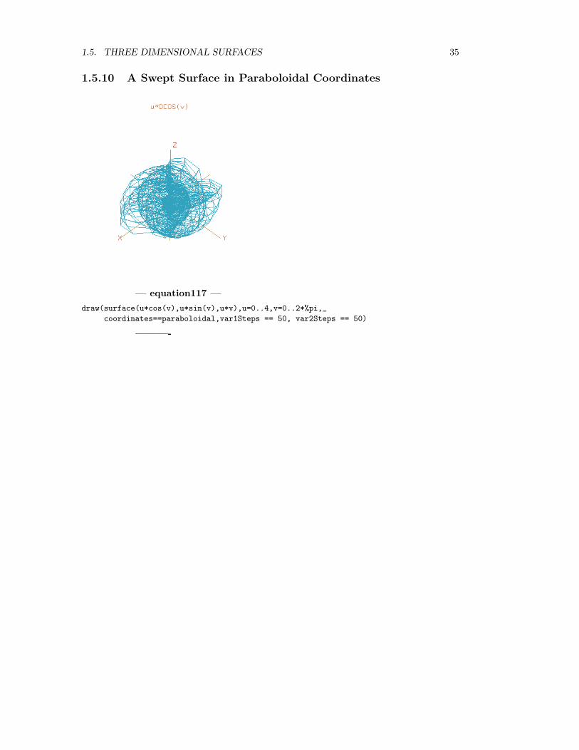
1.5.10 A Swept Surface in Paraboloidal Coordinates
— equation117 —
draw(surface(u*cos(v),u*sin(v),u*v),u=0..4,v=0..2*%pi,_
coordinates==paraboloidal,var1Steps == 50, var2Steps == 50)
———-

36 CHAPTER 1. GENERAL EXAMPLES

Chapter 2
Jenks Book images
37

38 CHAPTER 2. JENKS BOOK IMAGES
2.0.11 The Complex Gamma Function
— complexgamma —
gam(x:DoubleFloat,y:DoubleFloat):Point(DoubleFloat) == _
( g:Complex(DoubleFloat):= Gamma complex(x,y) ; _
point [x,y,max(min(real g, 4), -4), argument g] )
v3d:=draw(gam, -%pi..%pi, -%pi..%pi, title == "Gamma(x + %i*y)", _
var1Steps == 100, var2Steps == 100, style=="smooth")
———-
A 3-d surface whose height is the real part of the Gamma function, and whose color is theargument of the Gamma function.

39
2.0.12 The Complex Arctangent Function
— complexarctangent —
atf(x:DoubleFloat,y:DoubleFloat):Point(DoubleFloat) == _
( a := atan complex(x,y) ; _
point [x,y,real a, argument a] )
v3d:=draw(atf, -3.0..%pi, -3.0..%pi, style=="shade")
rotate(v3d,210,-60)
———-
The complex arctangent function. The height is the real part and the color is the argument.

40 CHAPTER 2. JENKS BOOK IMAGES
Chapter 3
Hyperdoc examples
Examples in this section come from the Hyperdoc documentation tool. These examples areaccessed from the Basic Examples Draw section.
3.1 Two dimensional examples
41

42 CHAPTER 3. HYPERDOC EXAMPLES
3.1.1 A function of one variable
— equation001 —
draw(x*cos(x),x=0..30,title=="y = x*cos(x)")
———-
This is one of the demonstration equations used in hypertex. It demonstrates a function ofone variable. It draws
y = f(x)
where y is the dependent variable and x is the independent variable.

3.1. TWO DIMENSIONAL EXAMPLES 43
3.1.2 A Parametric function
— equation002 —
draw(curve(-9*sin(4*t/5),8*sin(t)),t=-5*%pi..5*%pi,title=="Lissajous")
———-
This is one of the demonstration equations used in hypertex. It draw a parametrically definedcurve
f1(t), f2(t)
in terms of two functions f1 and f2 and an independent variable t.

44 CHAPTER 3. HYPERDOC EXAMPLES
3.1.3 A Polynomial in 2 variables
— equation003 —
draw(y**2+7*x*y-(x**3+16*x) = 0,x,y,range==[-15..10,-10..50])
———-
This is one of the demonstration equations used in hypertex. Plotting the solution to
p(x, y) = 0
where p is a polynomial in two variables x and y.
3.2 Three dimensional examples

3.2. THREE DIMENSIONAL EXAMPLES 45
3.2.1 A function of two variables
— equation004 —
cf(x,y) == 0.5
draw(exp(cos(x-y)-sin(x*y))-2,x=-5..5,y=-5..5,_
colorFunction==cf,style=="smooth")
———-
This is one of the demonstration equations used in hypertex. A function of two variables
z = f(x, y)
where z is the dependent variable and where x and y are the dependent variables.

46 CHAPTER 3. HYPERDOC EXAMPLES
3.2.2 A parametrically defined curve
— equation005 —
f1(t) == 1.3*cos(2*t)*cos(4*t)+sin(4*t)*cos(t)
f2(t) == 1.3*sin(2*t)*cos(4*t)-sin(4*t)*sin(t)
f3(t) == 2.5*cos(4*t)
cf(x,y) == 0.5
draw(curve(f1(t),f2(t),f3(t)),t=0..4*%pi,tubeRadius==.25,tubePoints==16,_
title=="knot",colorFunction==cf,style=="smooth")
———-
This is one of the demonstration equations used in hypertex. This ia parametrically definedcurve
f1(t), f2(t), f3(t)
in terms of three functions f1, f2, and f3 and an independent variable t.

3.2. THREE DIMENSIONAL EXAMPLES 47
3.2.3 A parametrically defined surface
— equation006 —
f1(u,v) == u*sin(v)
f2(u,v) == v*cos(u)
f3(u,v) == u*cos(v)
cf(x,y) == 0.5
draw(surface(f1(u,v),f2(u,v),f3(u,v)),u=-%pi..%pi,v=-%pi/2..%pi/2,_
title=="surface",colorFunction==cf,style=="smooth")
———-
This is one of the demonstration equations used in hypertex. This ia parametrically definedcurve
f1(t), f2(t), f3(t)
in terms of three functions f1, f2, and f3 and an independent variable t.

48 CHAPTER 3. HYPERDOC EXAMPLES

Chapter 4
CRC Standard Curves andSurfaces
4.1 Standard Curves and Surfaces
In order to have an organized and thorough evaluation of the Axiom graphics code we turnto the CRC Standard Curves and Surfaces [Segg93] (SCC). This volume was written yearsafter the Axiom graphics code was written so there was no attempt to match the two untilnow. However, the SCC volume will give us a solid foundation to both evaluate the featuresof the current code and suggest future directions.
According to the SCC we can organize the various curves by the taxonomy:
1 random
1.1 fractal
1.2 gaussian
1.3 non-gaussian
2 determinate
2.1 algebraic – A polynomial is defined as a summation of terms composed of integralpowers of x and y. An algebraic curve is one whose implicit function
f(x, y) = 0
is a polynomial in x and y (after rationalization, if necessary). Because a curveis often defined in the explicit form
y = f(x)
there is a need to distinguish rational and irrational functions of x.
2.1.1 irrational – An irrational function of x is a quotient of two polynomials, oneor both of which has a term (or terms) with power p/q, where p and q areintegers.
2.1.2 rational – A rational function of x is a quotient of two polynomials in x,both having only integer powers.
49

50 CHAPTER 4. CRC STANDARD CURVES AND SURFACES
2.1.2.1 polynomial
2.1.2.2 non-polynomial
2.2 integral – Certain continuous functions are not expressible in algebraic or tran-scendental forms but are familiar mathematical tools. These curves are equal tothe integrals of algebraic or transcendental curves by definition; examples includeBessel functions, Airy integrals, Fresnel integrals, and the error function.
2.3 transcendental – The transcendental curves cannot be expressed as polynomialsin x and y. These are curves containing one or more of the following forms:exponential (ex), logarithmic (log(x)), or trigonometric (sin(x), cos(x)).
2.3.1 exponential
2.3.2 logarithmic
2.3.3 trigonometric
2.4 piecewise continuous – Other curves, except at a few singular points, aresmooth and differentiable. The class of nondifferentiable curves have disconti-nuity of the first derivative as a basic attribute. They are often composed ofstraight-line segments. Simple polygonal forms, regular fractal curves, and turtletracks are examples.
2.4.1 periodic
2.4.2 non-periodic
2.4.3 polygonal
2.4.3.1 regular
2.4.3.2 irregular
2.4.3.3 fractal
4.2 CRC graphs
4.2.1 Functions with xn/m

4.2. CRC GRAPHS 51
Page 26 2.1.1
y = cxn
y − cxn = 0
— p26-2.1.1.1-3 —
)clear all
)set mes auto off
f(c,x,n) == c*x^n
lineColorDefault(green())
viewport1:=draw(f(1,x,1), x=-2..2, adaptive==true, unit==[1.0,1.0],_
title=="p26-2.1.1.1-3")
graph2111:=getGraph(viewport1,1)
lineColorDefault(blue())
viewport2:=draw(f(1,x,3), x=-2..2, adaptive==true, unit==[1.0,1.0])
graph2112:=getGraph(viewport2,1)
lineColorDefault(red())
viewport3:=draw(f(1,x,5), x=-2..2, adaptive==true, unit==[1.0,1.0])
graph2113:=getGraph(viewport3,1)
putGraph(viewport1,graph2112,2)
putGraph(viewport1,graph2113,3)
units(viewport1,1,"on")
points(viewport1,1,"off")
points(viewport1,2,"off")
points(viewport1,3,"off")
makeViewport2D(viewport1)
———-

52 CHAPTER 4. CRC STANDARD CURVES AND SURFACES
— p26-2.1.1.4-6 —
)clear all
)set mes auto off
f(c,x,n) == c*x^n
lineColorDefault(green())
viewport1:=draw(f(1,x,2), x=-2..2, adaptive==true, unit==[1.0,1.0],_
title=="p26-2.1.1.4-6")
graph2111:=getGraph(viewport1,1)
lineColorDefault(blue())
viewport2:=draw(f(1,x,4), x=-2..2, adaptive==true, unit==[1.0,1.0])
graph2112:=getGraph(viewport2,1)
lineColorDefault(red())
viewport3:=draw(f(1,x,6), x=-2..2, adaptive==true, unit==[1.0,1.0])
graph2113:=getGraph(viewport3,1)
putGraph(viewport1,graph2112,2)
putGraph(viewport1,graph2113,3)
units(viewport1,1,"on")
points(viewport1,1,"off")
points(viewport1,2,"off")
points(viewport1,3,"off")
makeViewport2D(viewport1)
———-

4.2. CRC GRAPHS 53
Page 26 2.1.2
y =c
xn
yxn − c = 0
— p26-2.1.2.1-3 —
)clear all
f(c,x,n) == c/x^n
lineColorDefault(green())
viewport1:=draw(f(0.01,x,1),x=-2..2,adaptive==true,unit==[1.0,1.0],_
title=="p26-2.1.2.1-3")
graph2111:=getGraph(viewport1,1)
lineColorDefault(blue())
viewport2:=draw(f(0.01,x,3),x=-4..4,adaptive==true,unit==[1.0,1.0])
graph2122:=getGraph(viewport2,1)
lineColorDefault(red())
viewport3:=draw(f(0.01,x,5),x=-2..2,adaptive==true,unit==[1.0,1.0])
graph2123:=getGraph(viewport3,1)
putGraph(viewport1,graph2122,2)
putGraph(viewport1,graph2123,3)
units(viewport1,1,"on")
points(viewport1,1,"off")
points(viewport1,2,"off")
points(viewport1,3,"off")
makeViewport2D(viewport1)
———-

54 CHAPTER 4. CRC STANDARD CURVES AND SURFACES
Note that Axiom’s plot of viewport2 disagrees with CRC— p26-2.1.2.4-6 —
)clear all
f(c,x,n) == c/x^n
lineColorDefault(green())
viewport1:=draw(f(0.01,x,4),x=-2..2,adaptive==true,unit==[1.0,1.0],_
title=="p26-2.1.2.4-6")
graph2124:=getGraph(viewport1,1)
lineColorDefault(blue())
viewport2:=draw(f(0.01,x,5),x=-2..2,adaptive==true,unit==[1.0,1.0])
graph2125:=getGraph(viewport2,1)
lineColorDefault(red())
viewport3:=draw(f(0.01,x,6),x=-2..2,adaptive==true,unit==[1.0,1.0])
graph2126:=getGraph(viewport3,1)
putGraph(viewport1,graph2125,2)
putGraph(viewport1,graph2126,3)
units(viewport1,1,"on")
points(viewport1,1,"off")
points(viewport1,2,"off")
points(viewport1,3,"off")
makeViewport2D(viewport1)
———-
4.2. CRC GRAPHS 55
Page 28 2.1.3
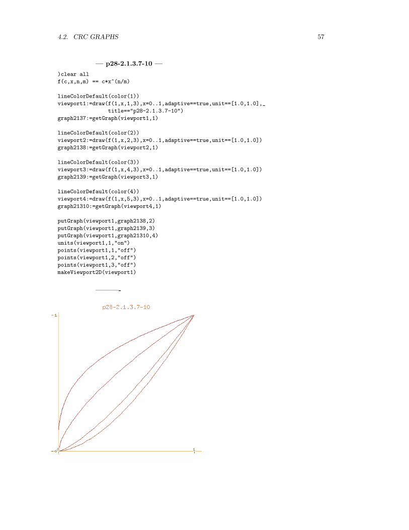
y = cxn/m
y − cxn/m = 0
— p28-2.1.3.1-6 —
)clear all
f(c,x,n,m) == c*x^(n/m)
lineColorDefault(color(1))
viewport1:=draw(f(1,x,1,4),x=0..1,adaptive==true,unit==[1.0,1.0],_
title=="p28-2.1.3.1-6")
graph2131:=getGraph(viewport1,1)
lineColorDefault(color(2))
viewport2:=draw(f(1,x,1,2),x=0..1,adaptive==true,unit==[1.0,1.0])
graph2132:=getGraph(viewport2,1)
lineColorDefault(color(3))
viewport3:=draw(f(1,x,3,4),x=0..1,adaptive==true,unit==[1.0,1.0])
graph2133:=getGraph(viewport3,1)
lineColorDefault(color(4))
viewport4:=draw(f(1,x,5,4),x=0..1,adaptive==true,unit==[1.0,1.0])
graph2134:=getGraph(viewport4,1)
lineColorDefault(color(5))
viewport5:=draw(f(1,x,3,2),x=0..1,adaptive==true,unit==[1.0,1.0])
graph2135:=getGraph(viewport5,1)
lineColorDefault(color(6))
viewport6:=draw(f(1,x,7,4),x=0..1,adaptive==true,unit==[1.0,1.0])
graph2136:=getGraph(viewport6,1)
putGraph(viewport1,graph2132,2)
putGraph(viewport1,graph2133,3)
putGraph(viewport1,graph2134,4)
putGraph(viewport1,graph2135,5)
putGraph(viewport1,graph2136,6)
units(viewport1,1,"on")
points(viewport1,1,"off")
points(viewport1,2,"off")
points(viewport1,3,"off")
makeViewport2D(viewport1)
———-

56 CHAPTER 4. CRC STANDARD CURVES AND SURFACES
4.2. CRC GRAPHS 57
— p28-2.1.3.7-10 —
)clear all
f(c,x,n,m) == c*x^(n/m)
lineColorDefault(color(1))
viewport1:=draw(f(1,x,1,3),x=0..1,adaptive==true,unit==[1.0,1.0],_
title=="p28-2.1.3.7-10")
graph2137:=getGraph(viewport1,1)
lineColorDefault(color(2))
viewport2:=draw(f(1,x,2,3),x=0..1,adaptive==true,unit==[1.0,1.0])
graph2138:=getGraph(viewport2,1)
lineColorDefault(color(3))
viewport3:=draw(f(1,x,4,3),x=0..1,adaptive==true,unit==[1.0,1.0])
graph2139:=getGraph(viewport3,1)
lineColorDefault(color(4))
viewport4:=draw(f(1,x,5,3),x=0..1,adaptive==true,unit==[1.0,1.0])
graph21310:=getGraph(viewport4,1)
putGraph(viewport1,graph2138,2)
putGraph(viewport1,graph2139,3)
putGraph(viewport1,graph21310,4)
units(viewport1,1,"on")
points(viewport1,1,"off")
points(viewport1,2,"off")
points(viewport1,3,"off")
makeViewport2D(viewport1)
———-

58 CHAPTER 4. CRC STANDARD CURVES AND SURFACES
Page 28 2.1.4
y =c
xn/m
yxn/m − c = 0
— p28-2.1.4.1-6 —
)clear all
f(c,x,n,m) == c/x^(n/m)
lineColorDefault(color(1))
viewport1:=draw(f(0.01,x,1,4),x=0..1,adaptive==true,unit==[1.0,1.0],_
title=="p28-2.1.4.1-6")
graph2141:=getGraph(viewport1,1)
lineColorDefault(color(2))
viewport2:=draw(f(0.01,x,1,2),x=0..1,adaptive==true,unit==[1.0,1.0])
graph2142:=getGraph(viewport2,1)
lineColorDefault(color(3))
viewport3:=draw(f(0.01,x,3,4),x=0..1,adaptive==true,unit==[1.0,1.0])
graph2143:=getGraph(viewport3,1)
lineColorDefault(color(4))
viewport4:=draw(f(0.01,x,5,4),x=0..1,adaptive==true,unit==[1.0,1.0])
graph2144:=getGraph(viewport4,1)
lineColorDefault(color(5))
viewport5:=draw(f(0.01,x,3,2),x=0..1,adaptive==true,unit==[1.0,1.0])
graph2145:=getGraph(viewport5,1)
lineColorDefault(color(6))
viewport6:=draw(f(0.01,x,7,4),x=0..1,adaptive==true,unit==[1.0,1.0])
graph2146:=getGraph(viewport6,1)
putGraph(viewport1,graph2142,2)
putGraph(viewport1,graph2143,3)
putGraph(viewport1,graph2144,4)
putGraph(viewport1,graph2145,5)
putGraph(viewport1,graph2146,6)
units(viewport1,1,"on")
points(viewport1,1,"off")
points(viewport1,2,"off")
points(viewport1,3,"off")
makeViewport2D(viewport1)
———-

4.2. CRC GRAPHS 59

60 CHAPTER 4. CRC STANDARD CURVES AND SURFACES
— p28-2.1.4.7-10 —
)clear all
f(c,x,n,m) == c/x^(n/m)
lineColorDefault(color(1))
viewport1:=draw(f(1,x,1,3),x=0..1,adaptive==true,unit==[1.0,1.0],_
title=="p28-2.1.4.7-10")
graph2147:=getGraph(viewport1,1)
lineColorDefault(color(2))
viewport2:=draw(f(1,x,2,3),x=0..1,adaptive==true,unit==[1.0,1.0])
graph2148:=getGraph(viewport2,1)
lineColorDefault(color(3))
viewport3:=draw(f(1,x,4,3),x=0..1,adaptive==true,unit==[1.0,1.0])
graph2149:=getGraph(viewport3,1)
lineColorDefault(color(4))
viewport4:=draw(f(1,x,5,3),x=0..1,adaptive==true,unit==[1.0,1.0])
graph21410:=getGraph(viewport4,1)
putGraph(viewport1,graph2148,2)
putGraph(viewport1,graph2149,3)
putGraph(viewport1,graph21410,4)
units(viewport1,1,"on")
points(viewport1,1,"off")
points(viewport1,2,"off")
points(viewport1,3,"off")
makeViewport2D(viewport1)
———-

4.2. CRC GRAPHS 61
4.2.2 Functions with xn and (a+ bx)m
Page 30 2.2.1
y = c(a+ bx)
y − bcx− ac = 0
— p30-2.2.1.1-3 —
)clear all
f(x,a,b,c) == c*(a+b*x)
lineColorDefault(red())
viewport1:=draw(f(x,0.5,0.5,1.0),x=-2..1,adaptive==true,unit==[1.0,1.0],_
title=="p30-2.2.1.1-3")
graph2211:=getGraph(viewport1,1)
lineColorDefault(green())
viewport2:=draw(f(x,0.5,1.0,1.0),x=-2..1,adaptive==true,unit==[1.0,1.0])
graph2212:=getGraph(viewport2,1)
lineColorDefault(blue())
viewport3:=draw(f(x,0.5,2.0,1.0),x=-2..1,adaptive==true,unit==[1.0,1.0])
graph2213:=getGraph(viewport3,1)
putGraph(viewport1,graph2212,2)
putGraph(viewport1,graph2213,3)
units(viewport1,1,"on")
points(viewport1,1,"off")
points(viewport1,2,"off")
points(viewport1,3,"off")
makeViewport2D(viewport1)
———-

62 CHAPTER 4. CRC STANDARD CURVES AND SURFACES

4.2. CRC GRAPHS 63
Page 30 2.2.2
y = c(a+ bx)2
y − cb2x2 − 2abcx− a2c = 0
— p30-2.2.2.1-3 —
)clear all
f(x,a,b,c) == c*(a+b*x)^2
lineColorDefault(red())
viewport1:=draw(f(x,0.5,0.5,1.0),x=-2..1,adaptive==true,unit==[1.0,1.0],_
title=="p30-2.2.2.1-3")
graph2221:=getGraph(viewport1,1)
lineColorDefault(green())
viewport2:=draw(f(x,0.5,1.0,1.0),x=-2..1,adaptive==true,unit==[1.0,1.0])
graph2222:=getGraph(viewport2,1)
lineColorDefault(blue())
viewport3:=draw(f(x,0.5,2.0,1.0),x=-2..1,adaptive==true,unit==[1.0,1.0])
graph2223:=getGraph(viewport3,1)
putGraph(viewport1,graph2222,2)
putGraph(viewport1,graph2223,3)
units(viewport1,1,"on")
points(viewport1,1,"off")
points(viewport1,2,"off")
points(viewport1,3,"off")
makeViewport2D(viewport1)
———-

64 CHAPTER 4. CRC STANDARD CURVES AND SURFACES
Page 30 2.2.3
y = c(a+ bx)3
y − b3cx3 − 3ab2cx2 − 3a2bcx− a3c = 0
— p30-2.2.3.1-3 —
)clear all
f(x,a,b,c) == c*(a+b*x)^3
lineColorDefault(red())
viewport1:=draw(f(x,0.5,0.5,1.0),x=-2..1,adaptive==true,unit==[1.0,1.0],_
title=="p30-2.2.3.1-3")
graph2231:=getGraph(viewport1,1)
lineColorDefault(green())
viewport2:=draw(f(x,0.5,1.0,1.0),x=-2..1,adaptive==true,unit==[1.0,1.0])
graph2232:=getGraph(viewport2,1)
lineColorDefault(blue())
viewport3:=draw(f(x,0.5,2.0,1.0),x=-2..1,adaptive==true,unit==[1.0,1.0])
graph2233:=getGraph(viewport3,1)
putGraph(viewport1,graph2232,2)
putGraph(viewport1,graph2233,3)
units(viewport1,1,"on")
points(viewport1,1,"off")
points(viewport1,2,"off")
points(viewport1,3,"off")
makeViewport2D(viewport1)
———-

4.2. CRC GRAPHS 65
Page 30 2.2.4
y = cx(a+ bx)
y − bcx2 − acx = 0
— p30-2.2.4.1-3 —
)clear all
f(x,a,b,c) == c*x*(a+b*x)
lineColorDefault(red())
viewport1:=draw(f(x,0.5,0.5,1.0),x=-2..1,adaptive==true,unit==[1.0,1.0],_
title=="p30-2.2.4.1-3")
graph2241:=getGraph(viewport1,1)
lineColorDefault(green())
viewport2:=draw(f(x,0.5,1.0,1.0),x=-2..1,adaptive==true,unit==[1.0,1.0])
graph2242:=getGraph(viewport2,1)
lineColorDefault(blue())
viewport3:=draw(f(x,0.5,2.0,1.0),x=-2..1,adaptive==true,unit==[1.0,1.0])
graph2243:=getGraph(viewport3,1)
putGraph(viewport1,graph2242,2)
putGraph(viewport1,graph2243,3)
units(viewport1,1,"on")
points(viewport1,1,"off")
points(viewport1,2,"off")
points(viewport1,3,"off")
makeViewport2D(viewport1)
———-

66 CHAPTER 4. CRC STANDARD CURVES AND SURFACES
Page 30 2.2.5
y = cx(a+ bx)2
y − b2cx3 − 2abcx2 − a2cx = 0
— p30-2.2.5.1-3 —
)clear all
f(x,a,b,c) == c*x*(a+b*x)^2
lineColorDefault(red())
viewport1:=draw(f(x,0.5,0.5,1.0),x=-2..1,adaptive==true,unit==[1.0,1.0],_
title=="p30-2.2.5.1-3")
graph2251:=getGraph(viewport1,1)
lineColorDefault(green())
viewport2:=draw(f(x,0.5,1.0,1.0),x=-2..1,adaptive==true,unit==[1.0,1.0])
graph2252:=getGraph(viewport2,1)
lineColorDefault(blue())
viewport3:=draw(f(x,0.5,2.0,1.0),x=-2..1,adaptive==true,unit==[1.0,1.0])
graph2253:=getGraph(viewport3,1)
putGraph(viewport1,graph2252,2)
putGraph(viewport1,graph2253,3)
units(viewport1,1,"on")
points(viewport1,1,"off")
points(viewport1,2,"off")
points(viewport1,3,"off")
makeViewport2D(viewport1)
———-

4.2. CRC GRAPHS 67
Page 30 2.2.6
y = cx(a+ bx)3
y − b3cx4 − 3ab2cx3 − 3a2bcx2 − a3cx = 0
— p30-2.2.6.1-3 —
)clear all
f(x,a,b,c) == c*x*(a+b*x)^3
lineColorDefault(red())
viewport1:=draw(f(x,0.5,0.5,1.0),x=-2..1,adaptive==true,unit==[1.0,1.0],_
title=="p30-2.2.6.1-3")
graph2261:=getGraph(viewport1,1)
lineColorDefault(green())
viewport2:=draw(f(x,0.5,1.0,1.0),x=-2..1,adaptive==true,unit==[1.0,1.0])
graph2262:=getGraph(viewport2,1)
lineColorDefault(blue())
viewport3:=draw(f(x,0.5,2.0,1.0),x=-2..1,adaptive==true,unit==[1.0,1.0])
graph2263:=getGraph(viewport3,1)
putGraph(viewport1,graph2262,2)
putGraph(viewport1,graph2263,3)
units(viewport1,1,"on")
points(viewport1,1,"off")
points(viewport1,2,"off")
points(viewport1,3,"off")
makeViewport2D(viewport1)
———-

68 CHAPTER 4. CRC STANDARD CURVES AND SURFACES
Page 32 2.2.7
y = cx2(a+ bx)
y − bcx3 − acx2 = 0
— p32-2.2.7.1-3 —
)clear all
f(x,a,b,c) == c*x^2*(a+b*x)
lineColorDefault(red())
viewport1:=draw(f(x,0.5,0.5,1.0),x=-2..1,adaptive==true,unit==[1.0,1.0],_
title=="p30-2.2.7.1-3")
graph2271:=getGraph(viewport1,1)
lineColorDefault(green())
viewport2:=draw(f(x,0.5,1.0,1.0),x=-2..1,adaptive==true,unit==[1.0,1.0])
graph2272:=getGraph(viewport2,1)
lineColorDefault(blue())
viewport3:=draw(f(x,0.5,2.0,1.0),x=-2..1,adaptive==true,unit==[1.0,1.0])
graph2273:=getGraph(viewport3,1)
putGraph(viewport1,graph2272,2)
putGraph(viewport1,graph2273,3)
units(viewport1,1,"on")
points(viewport1,1,"off")
points(viewport1,2,"off")
points(viewport1,3,"off")
makeViewport2D(viewport1)
———-

4.2. CRC GRAPHS 69
Page 32 2.2.8
y = cx2(a+ bx)2
y − b2cx4 − 2abcx3 − a2cx2 = 0
— p32-2.2.8.1-3 —
)clear all
f(x,a,b,c) == c*x^2*(a+b*x)^2
lineColorDefault(red())
viewport1:=draw(f(x,0.5,0.5,1.0),x=-2..1,adaptive==true,unit==[1.0,1.0],_
title=="p32-2.2.8.1-3")
graph2281:=getGraph(viewport1,1)
lineColorDefault(green())
viewport2:=draw(f(x,0.5,1.0,1.0),x=-2..1,adaptive==true,unit==[1.0,1.0])
graph2282:=getGraph(viewport2,1)
lineColorDefault(blue())
viewport3:=draw(f(x,0.5,2.0,1.0),x=-2..1,adaptive==true,unit==[1.0,1.0])
graph2283:=getGraph(viewport3,1)
putGraph(viewport1,graph2282,2)
putGraph(viewport1,graph2283,3)
units(viewport1,1,"on")
points(viewport1,1,"off")
points(viewport1,2,"off")
points(viewport1,3,"off")
makeViewport2D(viewport1)
———-

70 CHAPTER 4. CRC STANDARD CURVES AND SURFACES
Page 32 2.2.9
y = cx2(a+ bx)3
y − b3cx5 − 3ab2cx4 − 3a2bcx3 − a3cx2 = 0
— p32-2.2.9.1-3 —
)clear all
f(x,a,b,c) == c*x^2*(a+b*x)^3
lineColorDefault(red())
viewport1:=draw(f(x,0.5,0.5,1.0),x=-2..1,adaptive==true,unit==[1.0,1.0],_
title=="p32-2.2.9.1-3")
graph2291:=getGraph(viewport1,1)
lineColorDefault(green())
viewport2:=draw(f(x,0.5,1.0,1.0),x=-2..1,adaptive==true,unit==[1.0,1.0])
graph2292:=getGraph(viewport2,1)
lineColorDefault(blue())
viewport3:=draw(f(x,0.5,2.0,1.0),x=-2..1,adaptive==true,unit==[1.0,1.0])
graph2293:=getGraph(viewport3,1)
putGraph(viewport1,graph2292,2)
putGraph(viewport1,graph2293,3)
units(viewport1,1,"on")
points(viewport1,1,"off")
points(viewport1,2,"off")
points(viewport1,3,"off")
makeViewport2D(viewport1)
———-

4.2. CRC GRAPHS 71
Page 32 2.2.10
y = cx3(a+ bx)
y − bcx4 − acx3 = 0
— p32-2.2.10.1-3 —
)clear all
f(x,a,b,c) == c*x^3*(a+b*x)
lineColorDefault(red())
viewport1:=draw(f(x,0.5,0.5,1.0),x=-2..2,adaptive==true,unit==[1.0,1.0],_
title=="p32-2.2.10.1-3")
graph22101:=getGraph(viewport1,1)
lineColorDefault(green())
viewport2:=draw(f(x,0.5,1.0,1.0),x=-2..2,adaptive==true,unit==[1.0,1.0])
graph22102:=getGraph(viewport2,1)
lineColorDefault(blue())
viewport3:=draw(f(x,0.5,2.0,1.0),x=-2..2,adaptive==true,unit==[1.0,1.0])
graph22103:=getGraph(viewport3,1)
putGraph(viewport1,graph22102,2)
putGraph(viewport1,graph22103,3)
units(viewport1,1,"on")
points(viewport1,1,"off")
points(viewport1,2,"off")
points(viewport1,3,"off")
makeViewport2D(viewport1)
———-

72 CHAPTER 4. CRC STANDARD CURVES AND SURFACES
Page 32 2.2.11
y = cx3(a+ bx)2
y − b2cx5 − 2abcx4 − a2cx3 = 0
— p32-2.2.11.1-3 —
)clear all
f(x,a,b,c) == c*x^3*(a+b*x)^2
lineColorDefault(red())
viewport1:=draw(f(x,0.5,0.5,1.0),x=-2..2,adaptive==true,unit==[1.0,1.0],_
title=="p32-2.2.11.1-3")
graph22111:=getGraph(viewport1,1)
lineColorDefault(green())
viewport2:=draw(f(x,0.5,1.0,1.0),x=-2..2,adaptive==true,unit==[1.0,1.0])
graph22112:=getGraph(viewport2,1)
lineColorDefault(blue())
viewport3:=draw(f(x,0.5,2.0,1.0),x=-2..2,adaptive==true,unit==[1.0,1.0])
graph22113:=getGraph(viewport3,1)
putGraph(viewport1,graph22112,2)
putGraph(viewport1,graph22113,3)
units(viewport1,1,"on")
points(viewport1,1,"off")
points(viewport1,2,"off")
points(viewport1,3,"off")
makeViewport2D(viewport1)
———-

4.2. CRC GRAPHS 73
Page 32 2.2.12
y = cx3(a+ bx)3
y − b3cx6 − 3ab2cx5 − 3a2bcx4 − a3cx3 = 0
— p32-2.2.12.1-3 —
)clear all
f(x,a,b,c) == c*x^3*(a+b*x)^3
lineColorDefault(red())
viewport1:=draw(f(x,0.5,0.5,1.0),x=-2..2,adaptive==true,unit==[1.0,1.0],_
title=="p32-2.2.12.1-3")
graph22121:=getGraph(viewport1,1)
lineColorDefault(green())
viewport2:=draw(f(x,0.5,1.0,1.0),x=-2..2,adaptive==true,unit==[1.0,1.0])
graph22122:=getGraph(viewport2,1)
lineColorDefault(blue())
viewport3:=draw(f(x,0.5,2.0,1.0),x=-2..2,adaptive==true,unit==[1.0,1.0])
graph22123:=getGraph(viewport3,1)
putGraph(viewport1,graph22122,2)
putGraph(viewport1,graph22123,3)
units(viewport1,1,"on")
points(viewport1,1,"off")
points(viewport1,2,"off")
points(viewport1,3,"off")
makeViewport2D(viewport1)
———-
74 CHAPTER 4. CRC STANDARD CURVES AND SURFACES
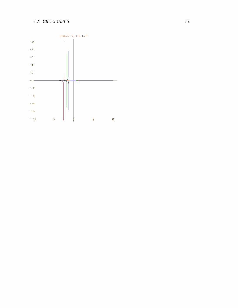
Page 34 2.2.13
y =c
(a+ bx)
ay + bxy − c = 0
— p34-2.2.13.1-3 —
)clear all
f(x,a,b,c) == c/(a+b*x)
lineColorDefault(red())
viewport1:=draw(f(x,1.0,2.0,0.02),x=-2..2,adaptive==true,unit==[1.0,1.0],_
title=="p34-2.2.13.1-3")
graph22131:=getGraph(viewport1,1)
lineColorDefault(green())
viewport2:=draw(f(x,1.0,3.0,0.02),x=-2..2,adaptive==true,unit==[1.0,1.0])
graph22132:=getGraph(viewport2,1)
lineColorDefault(blue())
viewport3:=draw(f(x,1.0,4.0,0.02),x=-2..2,adaptive==true,unit==[1.0,1.0])
graph22133:=getGraph(viewport3,1)
putGraph(viewport1,graph22132,2)
putGraph(viewport1,graph22133,3)
units(viewport1,1,"on")
points(viewport1,1,"off")
points(viewport1,2,"off")
points(viewport1,3,"off")
makeViewport2D(viewport1)
———-
4.2. CRC GRAPHS 75

76 CHAPTER 4. CRC STANDARD CURVES AND SURFACES
Page 34 2.2.14
y =c
(a+ bx)2
a2y + 2abxy + b2x2y − c = 0
— p34-2.2.14.1-3 —
)clear all
f(x,a,b,c) == c/(a+b*x)^2
lineColorDefault(red())
viewport1:=draw(f(x,1.0,2.0,0.02),x=-2..2,adaptive==true,unit==[1.0,1.0],_
title=="p34-2.2.14.1-3")
graph22141:=getGraph(viewport1,1)
lineColorDefault(green())
viewport2:=draw(f(x,1.0,3.0,0.02),x=-2..2,adaptive==true,unit==[1.0,1.0])
graph22142:=getGraph(viewport2,1)
lineColorDefault(blue())
viewport3:=draw(f(x,1.0,4.0,0.02),x=-2..2,adaptive==true,unit==[1.0,1.0])
graph22143:=getGraph(viewport3,1)
putGraph(viewport1,graph22142,2)
putGraph(viewport1,graph22143,3)
units(viewport1,1,"on")
points(viewport1,1,"off")
points(viewport1,2,"off")
points(viewport1,3,"off")
makeViewport2D(viewport1)
———-

4.2. CRC GRAPHS 77

78 CHAPTER 4. CRC STANDARD CURVES AND SURFACES
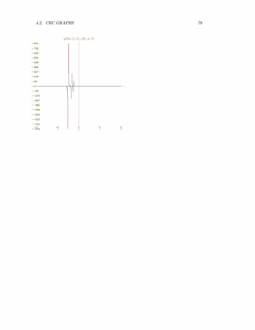
Page 34 2.2.15
y =c
(a+ bx)3
a3y + 2a2bxy + 2ab2x2y + b3x3y − c = 0
— p34-2.2.15.1-3 —
)clear all
f(x,a,b,c) == c/(a+b*x)^3
lineColorDefault(red())
viewport1:=draw(f(x,1.0,2.0,0.02),x=-2..2,adaptive==true,unit==[1.0,1.0],_
title=="p34-2.2.15.1-3")
graph22151:=getGraph(viewport1,1)
lineColorDefault(green())
viewport2:=draw(f(x,1.0,3.0,0.02),x=-2..2,adaptive==true,unit==[1.0,1.0])
graph22152:=getGraph(viewport2,1)
lineColorDefault(blue())
viewport3:=draw(f(x,1.0,4.0,0.02),x=-2..2,adaptive==true,unit==[1.0,1.0])
graph22153:=getGraph(viewport3,1)
putGraph(viewport1,graph22152,2)
putGraph(viewport1,graph22153,3)
units(viewport1,1,"on")
points(viewport1,1,"off")
points(viewport1,2,"off")
points(viewport1,3,"off")
makeViewport2D(viewport1)
———-
4.2. CRC GRAPHS 79

80 CHAPTER 4. CRC STANDARD CURVES AND SURFACES
Page 34 2.2.16
y =cx
(a+ bx)
ay + bxy − cx = 0
— p34-2.2.16.1-3 —
)clear all
f(x,a,b,c) == c*x/(a+b*x)
lineColorDefault(red())
viewport1:=draw(f(x,1.0,2.0,0.1),x=-2..2,adaptive==true,unit==[1.0,1.0],_
title=="p34-2.2.16.1-3")
graph22161:=getGraph(viewport1,1)
lineColorDefault(green())
viewport2:=draw(f(x,1.0,3.0,0.1),x=-2..2,adaptive==true,unit==[1.0,1.0])
graph22162:=getGraph(viewport2,1)
lineColorDefault(blue())
viewport3:=draw(f(x,1.0,4.0,0.1),x=-2..2,adaptive==true,unit==[1.0,1.0])
graph22163:=getGraph(viewport3,1)
putGraph(viewport1,graph22162,2)
putGraph(viewport1,graph22163,3)
units(viewport1,1,"on")
points(viewport1,1,"off")
points(viewport1,2,"off")
points(viewport1,3,"off")
makeViewport2D(viewport1)
———-

4.2. CRC GRAPHS 81

82 CHAPTER 4. CRC STANDARD CURVES AND SURFACES
Page 34 2.2.17
y =cx
(a+ bx)2
a2y + 2abxy + b2x2y − cx = 0
— p34-2.2.17.1-3 —
)clear all
f(x,a,b,c) == c*x/(a+b*x)^2
lineColorDefault(red())
viewport1:=draw(f(x,1.0,2.0,0.02),x=-2..2,adaptive==true,unit==[1.0,1.0],_
title=="p34-2.2.17.1-3")
graph22171:=getGraph(viewport1,1)
lineColorDefault(green())
viewport2:=draw(f(x,1.0,3.0,0.02),x=-2..2,adaptive==true,unit==[1.0,1.0])
graph22172:=getGraph(viewport2,1)
lineColorDefault(blue())
viewport3:=draw(f(x,1.0,4.0,0.02),x=-2..2,adaptive==true,unit==[1.0,1.0])
graph22173:=getGraph(viewport3,1)
putGraph(viewport1,graph22172,2)
putGraph(viewport1,graph22173,3)
units(viewport1,1,"on")
points(viewport1,1,"off")
points(viewport1,2,"off")
points(viewport1,3,"off")
makeViewport2D(viewport1)
———-

4.2. CRC GRAPHS 83

84 CHAPTER 4. CRC STANDARD CURVES AND SURFACES
Page 34 2.2.18
y =cx
(a+ bx)3
a3y + 3a2bxy + 3ab2x2y + b3x3y − cx = 0
— p34-2.2.18.1-3 —
)clear all
f(x,a,b,c) == c*x/(a+b*x)^3
lineColorDefault(red())
viewport1:=draw(f(x,1.0,2.0,0.01),x=-2..2,adaptive==true,unit==[1.0,1.0],_
title=="p34-2.2.18.1-3")
graph22181:=getGraph(viewport1,1)
lineColorDefault(green())
viewport2:=draw(f(x,1.0,3.0,0.01),x=-2..2,adaptive==true,unit==[1.0,1.0])
graph22182:=getGraph(viewport2,1)
lineColorDefault(blue())
viewport3:=draw(f(x,1.0,4.0,0.01),x=-2..2,adaptive==true,unit==[1.0,1.0])
graph22183:=getGraph(viewport3,1)
putGraph(viewport1,graph22182,2)
putGraph(viewport1,graph22183,3)
units(viewport1,1,"on")
points(viewport1,1,"off")
points(viewport1,2,"off")
points(viewport1,3,"off")
makeViewport2D(viewport1)
———-

4.2. CRC GRAPHS 85

86 CHAPTER 4. CRC STANDARD CURVES AND SURFACES
Page 36 2.2.19
y =cx2
(a+ bx)
ay + bxy − cx2 = 0
— p36-2.2.19.1-3 —
)clear all
f(x,a,b,c) == c*x^2/(a+b*x)
lineColorDefault(red())
viewport1:=draw(f(x,1.0,2.0,0.2),x=-2..2,adaptive==true,unit==[1.0,1.0],_
title=="p36-2.2.19.1-3")
graph22191:=getGraph(viewport1,1)
lineColorDefault(green())
viewport2:=draw(f(x,1.0,3.0,0.2),x=-2..2,adaptive==true,unit==[1.0,1.0])
graph22192:=getGraph(viewport2,1)
lineColorDefault(blue())
viewport3:=draw(f(x,1.0,4.0,0.2),x=-2..2,adaptive==true,unit==[1.0,1.0])
graph22193:=getGraph(viewport3,1)
putGraph(viewport1,graph22192,2)
putGraph(viewport1,graph22193,3)
units(viewport1,1,"on")
points(viewport1,1,"off")
points(viewport1,2,"off")
points(viewport1,3,"off")
makeViewport2D(viewport1)
———-

4.2. CRC GRAPHS 87

88 CHAPTER 4. CRC STANDARD CURVES AND SURFACES
Page 36 2.2.20
y =cx2
(a+ bx)2
a2y + 2abxy + b2x2y − cx2 = 0
— p36-2.2.20.1-3 —
)clear all
f(x,a,b,c) == c*x^2/(a+b*x)^2
lineColorDefault(red())
viewport1:=draw(f(x,1.0,2.0,0.1),x=-2..2,adaptive==true,unit==[1.0,1.0],_
title=="p36-2.2.20.1-3")
graph22201:=getGraph(viewport1,1)
lineColorDefault(green())
viewport2:=draw(f(x,1.0,3.0,0.1),x=-2..2,adaptive==true,unit==[1.0,1.0])
graph22202:=getGraph(viewport2,1)
lineColorDefault(blue())
viewport3:=draw(f(x,1.0,4.0,0.1),x=-2..2,adaptive==true,unit==[1.0,1.0])
graph22203:=getGraph(viewport3,1)
putGraph(viewport1,graph22202,2)
putGraph(viewport1,graph22203,3)
units(viewport1,1,"on")
points(viewport1,1,"off")
points(viewport1,2,"off")
points(viewport1,3,"off")
makeViewport2D(viewport1)
———-

4.2. CRC GRAPHS 89

90 CHAPTER 4. CRC STANDARD CURVES AND SURFACES
Page 36 2.2.21
y =cx2
(a+ bx)3
a3y + 3a2bxy + 3ab2x2y + b3x3y − cx2 = 0
— p36-2.2.21.1-3 —
)clear all
f(x,a,b,c) == c*x^2/(a+b*x)^3
lineColorDefault(red())
viewport1:=draw(f(x,1.0,2.0,0.02),x=-2..2,adaptive==true,unit==[1.0,1.0],_
title=="p36-2.2.21.1-3")
graph22211:=getGraph(viewport1,1)
lineColorDefault(green())
viewport2:=draw(f(x,1.0,3.0,0.02),x=-2..2,adaptive==true,unit==[1.0,1.0])
graph22212:=getGraph(viewport2,1)
lineColorDefault(blue())
viewport3:=draw(f(x,1.0,4.0,0.02),x=-2..2,adaptive==true,unit==[1.0,1.0])
graph22213:=getGraph(viewport3,1)
putGraph(viewport1,graph22212,2)
putGraph(viewport1,graph22213,3)
units(viewport1,1,"on")
points(viewport1,1,"off")
points(viewport1,2,"off")
points(viewport1,3,"off")
makeViewport2D(viewport1)
———-

4.2. CRC GRAPHS 91

92 CHAPTER 4. CRC STANDARD CURVES AND SURFACES
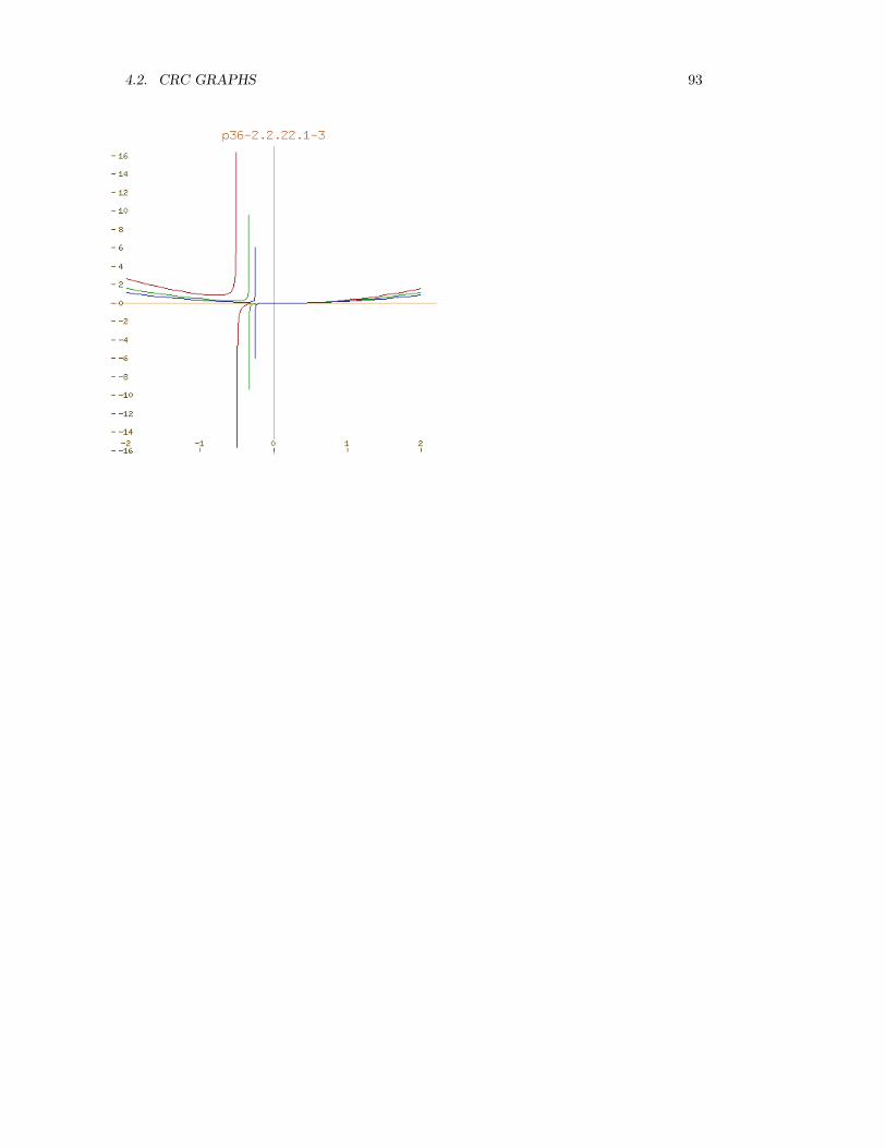
Page 36 2.2.22
y =cx3
(a+ bx)
ay + bxy − cx3 = 0
— p36-2.2.22.1-3 —
)clear all
f(x,a,b,c) == c*x^3/(a+b*x)
lineColorDefault(red())
viewport1:=draw(f(x,1.0,2.0,1.0),x=-2..2,adaptive==true,unit==[1.0,1.0],_
title=="p36-2.2.22.1-3")
graph22221:=getGraph(viewport1,1)
lineColorDefault(green())
viewport2:=draw(f(x,1.0,3.0,1.0),x=-2..2,adaptive==true,unit==[1.0,1.0])
graph22222:=getGraph(viewport2,1)
lineColorDefault(blue())
viewport3:=draw(f(x,1.0,4.0,1.0),x=-2..2,adaptive==true,unit==[1.0,1.0])
graph22223:=getGraph(viewport3,1)
putGraph(viewport1,graph22222,2)
putGraph(viewport1,graph22223,3)
units(viewport1,1,"on")
points(viewport1,1,"off")
points(viewport1,2,"off")
points(viewport1,3,"off")
makeViewport2D(viewport1)
———-
4.2. CRC GRAPHS 93

94 CHAPTER 4. CRC STANDARD CURVES AND SURFACES
Page 36 2.2.23
y =cx3
(a+ bx)2
a2y + 2abxy + b2x2y − cx3 = 0
— p36-2.2.23.1-3 —
)clear all
f(x,a,b,c) == c*x^3/(a+b*x)^2
lineColorDefault(red())
viewport1:=draw(f(x,1.0,2.0,0.2),x=-2..2,adaptive==true,unit==[1.0,1.0],_
title=="p36-2.2.23.1-3")
graph22231:=getGraph(viewport1,1)
lineColorDefault(green())
viewport2:=draw(f(x,1.0,3.0,0.2),x=-2..2,adaptive==true,unit==[1.0,1.0])
graph22232:=getGraph(viewport2,1)
lineColorDefault(blue())
viewport3:=draw(f(x,1.0,4.0,0.2),x=-2..2,adaptive==true,unit==[1.0,1.0])
graph22233:=getGraph(viewport3,1)
putGraph(viewport1,graph22232,2)
putGraph(viewport1,graph22233,3)
units(viewport1,1,"on")
points(viewport1,1,"off")
points(viewport1,2,"off")
points(viewport1,3,"off")
makeViewport2D(viewport1)
———-

4.2. CRC GRAPHS 95

96 CHAPTER 4. CRC STANDARD CURVES AND SURFACES
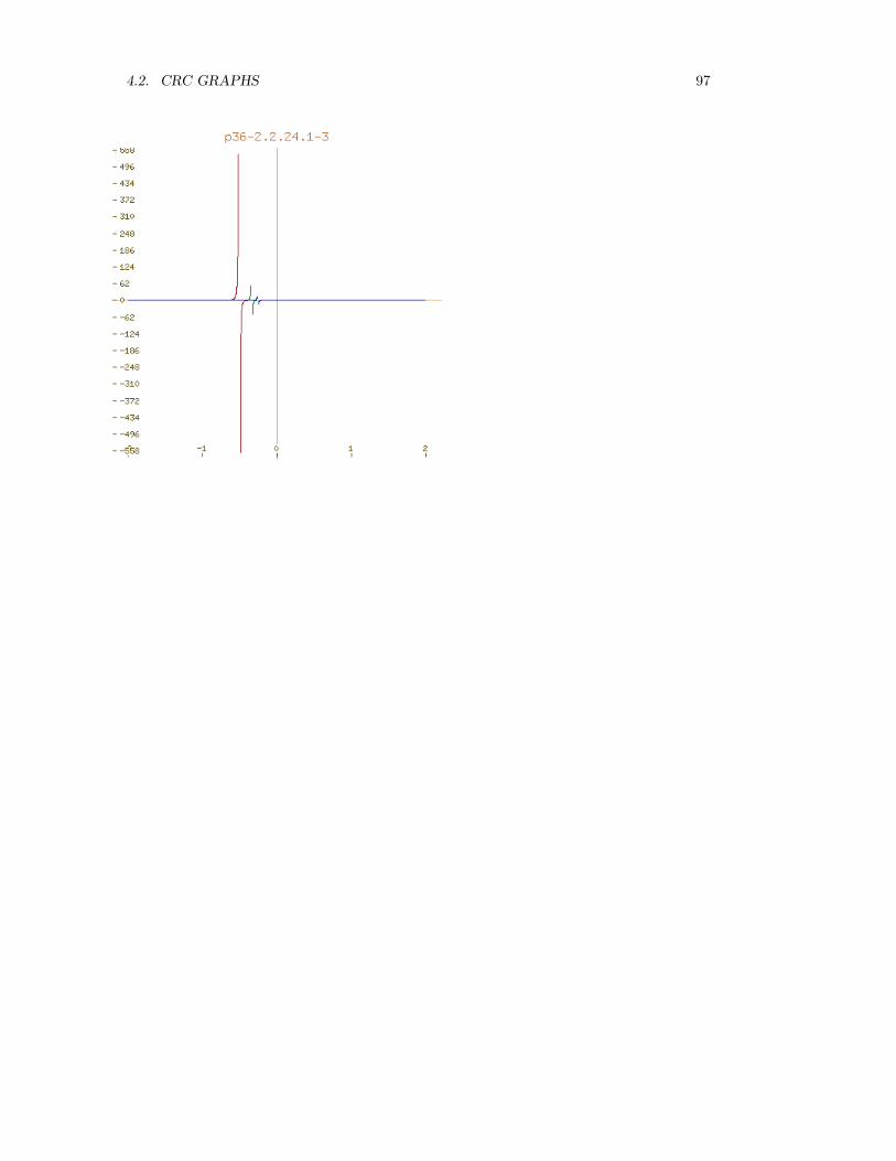
Page 36 2.2.24
y =cx3
(a+ bx)3
a3y + 3a2bxy + 3ab2x2y + b3x3y − cx3 = 0
— p36-2.2.24.1-3 —
)clear all
f(x,a,b,c) == c*x^3/(a+b*x)^3
lineColorDefault(red())
viewport1:=draw(f(x,1.0,2.0,0.1),x=-2..2,adaptive==true,unit==[1.0,1.0],_
title=="p36-2.2.24.1-3")
graph22241:=getGraph(viewport1,1)
lineColorDefault(green())
viewport2:=draw(f(x,1.0,3.0,0.1),x=-2..2,adaptive==true,unit==[1.0,1.0])
graph22242:=getGraph(viewport2,1)
lineColorDefault(blue())
viewport3:=draw(f(x,1.0,4.0,0.1),x=-2..2,adaptive==true,unit==[1.0,1.0])
graph22243:=getGraph(viewport3,1)
putGraph(viewport1,graph22242,2)
putGraph(viewport1,graph22243,3)
units(viewport1,1,"on")
points(viewport1,1,"off")
points(viewport1,2,"off")
points(viewport1,3,"off")
makeViewport2D(viewport1)
———-
4.2. CRC GRAPHS 97

98 CHAPTER 4. CRC STANDARD CURVES AND SURFACES
Page 38 2.2.25
y =c(a+ bx)
x
xy − bcx− ca = 0
— p38-2.2.25.1-3 —
)clear all
f(x,a,b,c) == c*(a+b*x)/x
lineColorDefault(red())
viewport1:=draw(f(x,1.0,2.0,0.04),x=-0.5..0.5,adaptive==true,unit==[1.0,1.0],_
title=="p38-2.2.25.1-3")
graph22251:=getGraph(viewport1,1)
lineColorDefault(green())
viewport2:=draw(f(x,1.0,4.0,0.04),x=-0.5..0.5,adaptive==true,unit==[1.0,1.0])
graph22252:=getGraph(viewport2,1)
lineColorDefault(blue())
viewport3:=draw(f(x,1.0,6.0,0.04),x=-0.5..0.5,adaptive==true,unit==[1.0,1.0])
graph22253:=getGraph(viewport3,1)
putGraph(viewport1,graph22252,2)
putGraph(viewport1,graph22253,3)
units(viewport1,1,"on")
points(viewport1,1,"off")
points(viewport1,2,"off")
points(viewport1,3,"off")
makeViewport2D(viewport1)
———-

4.2. CRC GRAPHS 99

100 CHAPTER 4. CRC STANDARD CURVES AND SURFACES
Page 38 2.2.26
y =c(a+ bx)2
x
xy − b2cx2 − 2abcx− a2c = 0
— p38-2.2.26.1-3 —
)clear all
f(x,a,b,c) == c*(a+b*x)^2/x
lineColorDefault(red())
viewport1:=draw(f(x,1.0,2.0,0.04),x=-2..2,adaptive==true,unit==[1.0,1.0],_
title=="p38-2.2.26.1-3")
graph22261:=getGraph(viewport1,1)
lineColorDefault(green())
viewport2:=draw(f(x,1.0,4.0,0.04),x=-2..2,adaptive==true,unit==[1.0,1.0])
graph22262:=getGraph(viewport2,1)
lineColorDefault(blue())
viewport3:=draw(f(x,1.0,6.0,0.04),x=-2..2,adaptive==true,unit==[1.0,1.0])
graph22263:=getGraph(viewport3,1)
putGraph(viewport1,graph22262,2)
putGraph(viewport1,graph22263,3)
units(viewport1,1,"on")
points(viewport1,1,"off")
points(viewport1,2,"off")
points(viewport1,3,"off")
makeViewport2D(viewport1)
———-

4.2. CRC GRAPHS 101

102 CHAPTER 4. CRC STANDARD CURVES AND SURFACES
Page 38 2.2.27
y =c(a+ bx)3
x
xy − b3cx3 − 3ab2cx2 − 3a2bcx− a3c = 0
— p38-2.2.27.1-3 —
)clear all
f(x,a,b,c) == c*(a+b*x)^3/x
lineColorDefault(red())
viewport1:=draw(f(x,1.0,2.0,0.02),x=-2..2,adaptive==true,unit==[1.0,1.0],_
title=="p38-2.2.27.1-3")
graph22271:=getGraph(viewport1,1)
lineColorDefault(green())
viewport2:=draw(f(x,1.0,4.0,0.02),x=-2..2,adaptive==true,unit==[1.0,1.0])
graph22272:=getGraph(viewport2,1)
lineColorDefault(blue())
viewport3:=draw(f(x,1.0,6.0,0.02),x=-2..2,adaptive==true,unit==[1.0,1.0])
graph22273:=getGraph(viewport3,1)
putGraph(viewport1,graph22272,2)
putGraph(viewport1,graph22273,3)
units(viewport1,1,"on")
points(viewport1,1,"off")
points(viewport1,2,"off")
points(viewport1,3,"off")
makeViewport2D(viewport1)
———-

4.2. CRC GRAPHS 103

104 CHAPTER 4. CRC STANDARD CURVES AND SURFACES
Page 38 2.2.28
y =c(a+ bx)
x2
x2y − bcx− ca = 0
— p38-2.2.28.1-3 —
)clear all
f(x,a,b,c) == c*(a+b*x)/x^2
lineColorDefault(red())
viewport1:=draw(f(x,1.0,2.0,0.04),x=-1..1,adaptive==true,unit==[1.0,1.0],_
title=="p38-2.2.28.1-3")
graph22281:=getGraph(viewport1,1)
lineColorDefault(green())
viewport2:=draw(f(x,1.0,4.0,0.04),x=-1..1,adaptive==true,unit==[1.0,1.0])
graph22282:=getGraph(viewport2,1)
lineColorDefault(blue())
viewport3:=draw(f(x,1.0,6.0,0.04),x=-1..1,adaptive==true,unit==[1.0,1.0])
graph22283:=getGraph(viewport3,1)
putGraph(viewport1,graph22282,2)
putGraph(viewport1,graph22283,3)
units(viewport1,1,"on")
points(viewport1,1,"off")
points(viewport1,2,"off")
points(viewport1,3,"off")
makeViewport2D(viewport1)
———-

4.2. CRC GRAPHS 105

106 CHAPTER 4. CRC STANDARD CURVES AND SURFACES
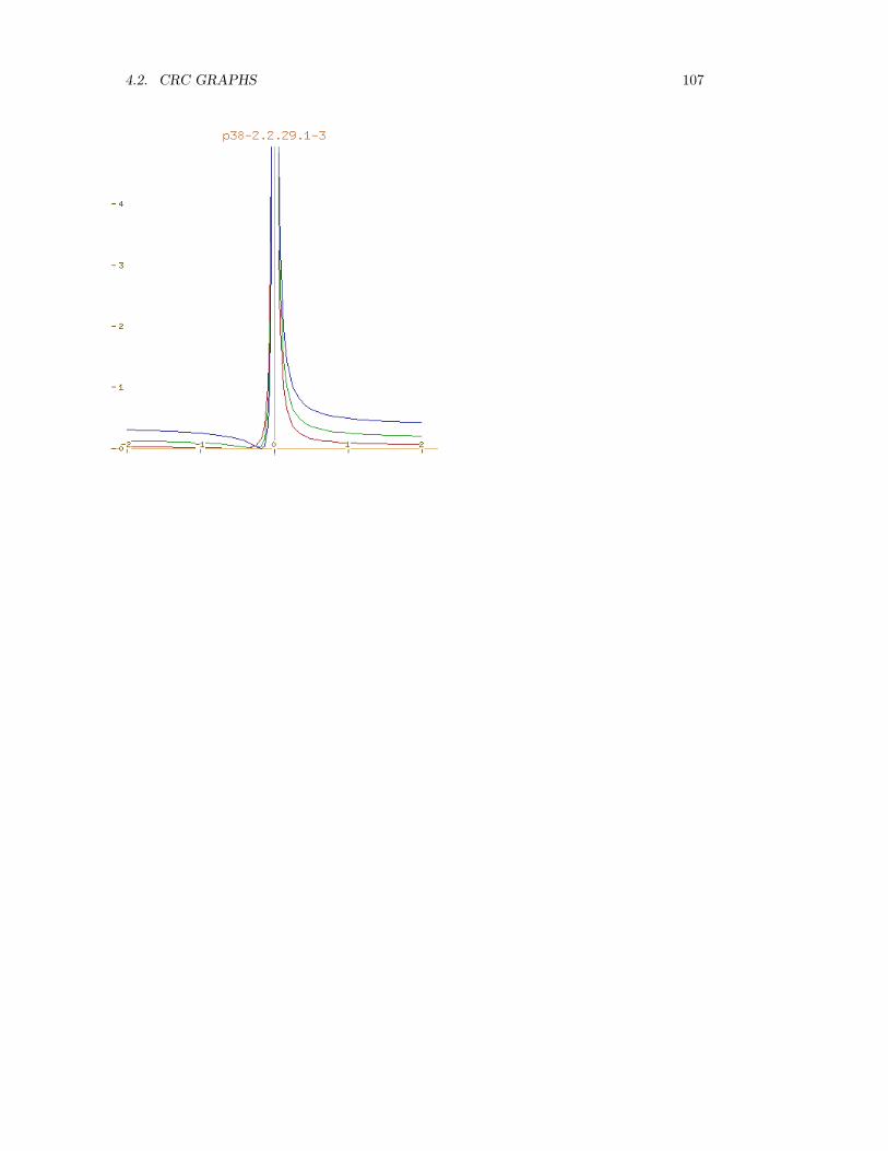
Page 38 2.2.29
y =c(a+ bx)2
x2
x2y − b2cx2 − 2abcx− a2c = 0
— p38-2.2.29.1-3 —
)clear all
f(x,a,b,c) == c*(a+b*x)^2/x^2
lineColorDefault(red())
viewport1:=draw(f(x,1.0,2.0,0.01),x=-2..2,adaptive==true,unit==[1.0,1.0],_
title=="p38-2.2.29.1-3")
graph22291:=getGraph(viewport1,1)
lineColorDefault(green())
viewport2:=draw(f(x,1.0,4.0,0.01),x=-2..2,adaptive==true,unit==[1.0,1.0])
graph22292:=getGraph(viewport2,1)
lineColorDefault(blue())
viewport3:=draw(f(x,1.0,6.0,0.01),x=-2..2,adaptive==true,unit==[1.0,1.0])
graph22293:=getGraph(viewport3,1)
putGraph(viewport1,graph22292,2)
putGraph(viewport1,graph22293,3)
units(viewport1,1,"on")
points(viewport1,1,"off")
points(viewport1,2,"off")
points(viewport1,3,"off")
makeViewport2D(viewport1)
———-
4.2. CRC GRAPHS 107

108 CHAPTER 4. CRC STANDARD CURVES AND SURFACES
Page 38 2.2.30
y =c(a+ bx)3
x2
x2y − b3cx3 − 3ab2cx2 − 3a2bcx− a3c = 0
— p38-2.2.30.1-3 —
)clear all
f(x,a,b,c) == c*(a+b*x)^3/x^2
lineColorDefault(red())
viewport1:=draw(f(x,1.0,2.0,0.003),x=-2..2,adaptive==true,unit==[1.0,1.0],_
title=="p38-2.2.30.1-3")
graph22301:=getGraph(viewport1,1)
lineColorDefault(green())
viewport2:=draw(f(x,1.0,4.0,0.003),x=-2..2,adaptive==true,unit==[1.0,1.0])
graph22302:=getGraph(viewport2,1)
lineColorDefault(blue())
viewport3:=draw(f(x,1.0,6.0,0.003),x=-2..2,adaptive==true,unit==[1.0,1.0])
graph22303:=getGraph(viewport3,1)
putGraph(viewport1,graph22302,2)
putGraph(viewport1,graph22303,3)
units(viewport1,1,"on")
points(viewport1,1,"off")
points(viewport1,2,"off")
points(viewport1,3,"off")
makeViewport2D(viewport1)
———-

4.2. CRC GRAPHS 109

110 CHAPTER 4. CRC STANDARD CURVES AND SURFACES
Page 40 2.2.31
y =c(a+ bx)
x3
x3y − bcx− ca = 0
— p40-2.2.31.1-3 —
)clear all
f(x,a,b,c) == c*(a+b*x)/x^3
lineColorDefault(red())
viewport1:=draw(f(x,1.0,2.0,0.02),x=-4..4,adaptive==true,unit==[1.0,1.0],_
title=="p40-2.2.31.1-3")
graph22311:=getGraph(viewport1,1)
lineColorDefault(green())
viewport2:=draw(f(x,1.0,4.0,0.02),x=-4..4,adaptive==true,unit==[1.0,1.0])
graph22312:=getGraph(viewport2,1)
lineColorDefault(blue())
viewport3:=draw(f(x,1.0,6.0,0.02),x=-4..4,adaptive==true,unit==[1.0,1.0])
graph22313:=getGraph(viewport3,1)
putGraph(viewport1,graph22312,2)
putGraph(viewport1,graph22313,3)
units(viewport1,1,"on")
points(viewport1,1,"off")
points(viewport1,2,"off")
points(viewport1,3,"off")
makeViewport2D(viewport1)
———-

4.2. CRC GRAPHS 111
112 CHAPTER 4. CRC STANDARD CURVES AND SURFACES
Page 40 2.2.32
y =c(a+ bx)2
x3
x3y − b2cx2 − 2abcx− a2c = 0
— p40-2.2.32.1-3 —
)clear all
f(x,a,b,c) == c*(a+b*x)^2/x^3
lineColorDefault(red())
viewport1:=draw(f(x,1.0,2.0,0.01),x=-2..2,adaptive==true,unit==[1.0,1.0],_
title=="p40-2.2.32.1-3")
graph22321:=getGraph(viewport1,1)
lineColorDefault(green())
viewport2:=draw(f(x,1.0,4.0,0.01),x=-2..2,adaptive==true,unit==[1.0,1.0])
graph22322:=getGraph(viewport2,1)
lineColorDefault(blue())
viewport3:=draw(f(x,1.0,6.0,0.01),x=-2..2,adaptive==true,unit==[1.0,1.0])
graph22323:=getGraph(viewport3,1)
putGraph(viewport1,graph22322,2)
putGraph(viewport1,graph22323,3)
units(viewport1,1,"on")
points(viewport1,1,"off")
points(viewport1,2,"off")
points(viewport1,3,"off")
makeViewport2D(viewport1)
———-

4.2. CRC GRAPHS 113

114 CHAPTER 4. CRC STANDARD CURVES AND SURFACES
Page 40 2.2.33
y =c(a+ bx)3
x3
x3y − b3cx3 − 3ab2cx2 − 3a2bcx− a3c = 0
— p40-2.2.33.1-3 —
)clear all
f(x,a,b,c) == c*(a+b*x)^3/x^3
lineColorDefault(red())
viewport1:=draw(f(x,1.0,2.0,0.002),x=-2..2,adaptive==true,unit==[1.0,1.0],_
title=="p40-2.2.33.1-3")
graph22331:=getGraph(viewport1,1)
lineColorDefault(green())
viewport2:=draw(f(x,1.0,4.0,0.002),x=-2..2,adaptive==true,unit==[1.0,1.0])
graph22332:=getGraph(viewport2,1)
lineColorDefault(blue())
viewport3:=draw(f(x,1.0,6.0,0.002),x=-2..2,adaptive==true,unit==[1.0,1.0])
graph22333:=getGraph(viewport3,1)
putGraph(viewport1,graph22332,2)
putGraph(viewport1,graph22333,3)
units(viewport1,1,"on")
points(viewport1,1,"off")
points(viewport1,2,"off")
points(viewport1,3,"off")
makeViewport2D(viewport1)
———-

4.2. CRC GRAPHS 115

116 CHAPTER 4. CRC STANDARD CURVES AND SURFACES
4.2.3 Functions with a2 + x2 and xm
Page 42 2.3.1
y =c
(a2 + b2)
a2y + x2y − c = 0
— p42-2.3.1.1-3 —
)clear all
f(x,a,c) == c/(a^2+x^2)
lineColorDefault(red())
viewport1:=draw(f(x,0.2,0.04),x=-2..2,adaptive==true,unit==[1.0,1.0],_
title=="p42-2.3.1.1-3")
graph1:=getGraph(viewport1,1)
lineColorDefault(green())
viewport2:=draw(f(x,0.5,0.04),x=-2..2,adaptive==true,unit==[1.0,1.0])
graph2:=getGraph(viewport2,1)
lineColorDefault(blue())
viewport3:=draw(f(x,0.8,0.04),x=-2..2,adaptive==true,unit==[1.0,1.0])
graph3:=getGraph(viewport3,1)
putGraph(viewport1,graph2,2)
putGraph(viewport1,graph3,3)
units(viewport1,1,"on")
points(viewport1,1,"off")
points(viewport1,2,"off")
points(viewport1,3,"off")
makeViewport2D(viewport1)
———-

4.2. CRC GRAPHS 117

118 CHAPTER 4. CRC STANDARD CURVES AND SURFACES
Page 42 2.3.2
y =cx
(a2 + b2)
a2y + x2y − cx = 0
— p42-2.3.2.1-3 —
)clear all
f(x,a,c) == c*x/(a^2+x^2)
lineColorDefault(red())
viewport1:=draw(f(x,0.2,0.3),x=-2..2,adaptive==true,unit==[1.0,1.0],_
title=="p42-2.3.2.1-3")
graph1:=getGraph(viewport1,1)
lineColorDefault(green())
viewport2:=draw(f(x,0.5,0.3),x=-2..2,adaptive==true,unit==[1.0,1.0])
graph2:=getGraph(viewport2,1)
lineColorDefault(blue())
viewport3:=draw(f(x,0.8,0.3),x=-2..2,adaptive==true,unit==[1.0,1.0])
graph3:=getGraph(viewport3,1)
putGraph(viewport1,graph2,2)
putGraph(viewport1,graph3,3)
units(viewport1,1,"on")
points(viewport1,1,"off")
points(viewport1,2,"off")
points(viewport1,3,"off")
makeViewport2D(viewport1)
———-

4.2. CRC GRAPHS 119
120 CHAPTER 4. CRC STANDARD CURVES AND SURFACES
Page 42 2.3.3
y =cx2
(a2 + b2)
a2y + x2y − cx2 = 0
— p42-2.3.3.1-3 —
)clear all
f(x,a,c) == c*x^2/(a^2+x^2)
lineColorDefault(red())
viewport1:=draw(f(x,0.2,1.0),x=-2..2,adaptive==true,unit==[1.0,1.0],_
title=="p42-2.3.3.1-3")
graph1:=getGraph(viewport1,1)
lineColorDefault(green())
viewport2:=draw(f(x,0.5,1.0),x=-2..2,adaptive==true,unit==[1.0,1.0])
graph2:=getGraph(viewport2,1)
lineColorDefault(blue())
viewport3:=draw(f(x,0.8,1.0),x=-2..2,adaptive==true,unit==[1.0,1.0])
graph3:=getGraph(viewport3,1)
putGraph(viewport1,graph2,2)
putGraph(viewport1,graph3,3)
units(viewport1,1,"on")
points(viewport1,1,"off")
points(viewport1,2,"off")
points(viewport1,3,"off")
makeViewport2D(viewport1)
———-
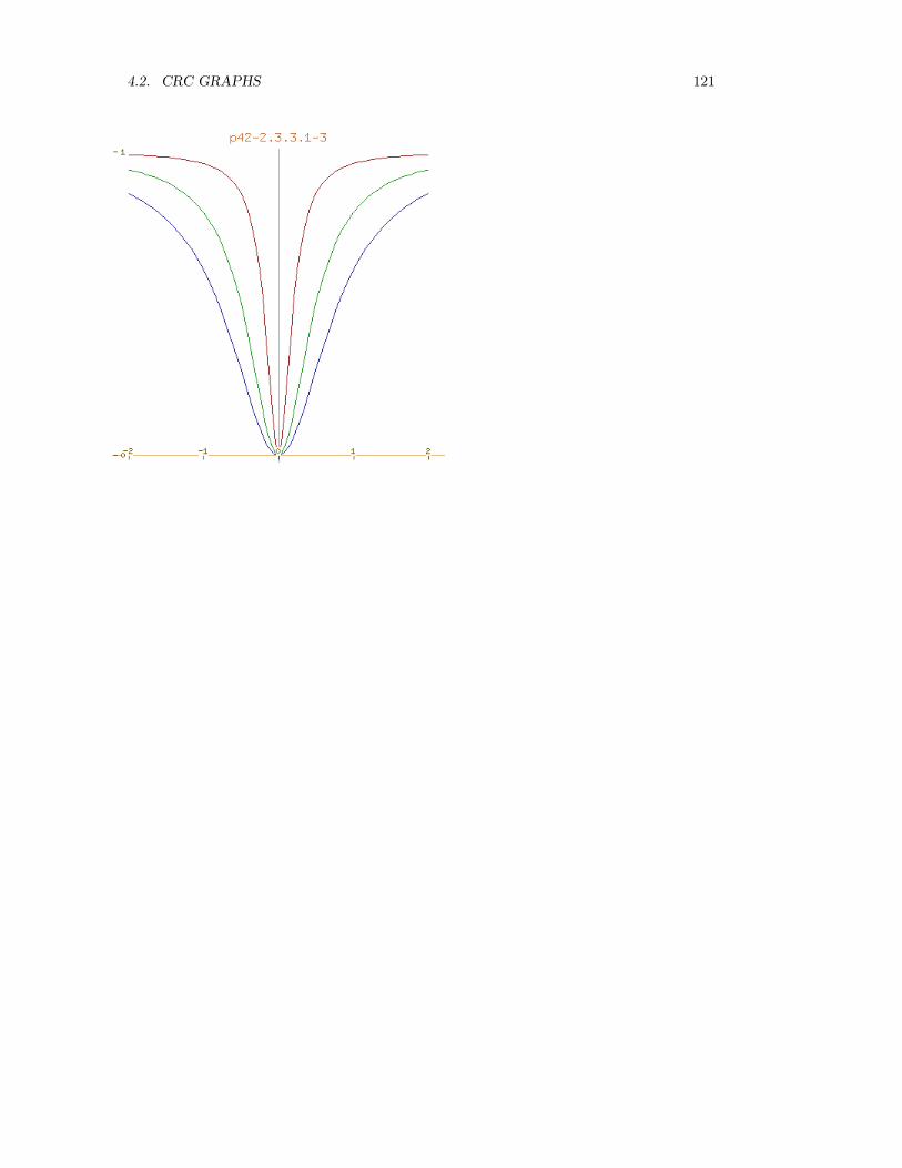
4.2. CRC GRAPHS 121

122 CHAPTER 4. CRC STANDARD CURVES AND SURFACES
Page 42 2.3.4
y =cx3
(a2 + b2)
a2y + x2y − cx3 = 0
— p42-2.3.4.1-3 —
)clear all
f(x,a,c) == c*x^3/(a^2+x^2)
lineColorDefault(red())
viewport1:=draw(f(x,0.2,1.0),x=-2..2,adaptive==true,unit==[1.0,1.0],_
title=="p42-2.3.4.1-3")
graph1:=getGraph(viewport1,1)
lineColorDefault(green())
viewport2:=draw(f(x,0.5,1.0),x=-2..2,adaptive==true,unit==[1.0,1.0])
graph2:=getGraph(viewport2,1)
lineColorDefault(blue())
viewport3:=draw(f(x,0.8,1.0),x=-2..2,adaptive==true,unit==[1.0,1.0])
graph3:=getGraph(viewport3,1)
putGraph(viewport1,graph2,2)
putGraph(viewport1,graph3,3)
units(viewport1,1,"on")
points(viewport1,1,"off")
points(viewport1,2,"off")
points(viewport1,3,"off")
makeViewport2D(viewport1)
———-

4.2. CRC GRAPHS 123

124 CHAPTER 4. CRC STANDARD CURVES AND SURFACES
Page 44 2.3.5
y =c
x(a2 + b2)
a2xy + x3y − c = 0
— p44-2.3.5.1-3 —
)clear all
f(x,a,c) == c/(x*(a^2+x^2))
lineColorDefault(red())
viewport1:=draw(f(x,0.2,1.0),x=-2..2,adaptive==true,unit==[1.0,1.0],_
title=="p44-2.3.5.1-3")
graph1:=getGraph(viewport1,1)
lineColorDefault(green())
viewport2:=draw(f(x,0.5,1.0),x=-2..2,adaptive==true,unit==[1.0,1.0])
graph2:=getGraph(viewport2,1)
lineColorDefault(blue())
viewport3:=draw(f(x,0.8,1.0),x=-2..2,adaptive==true,unit==[1.0,1.0])
graph3:=getGraph(viewport3,1)
putGraph(viewport1,graph2,2)
putGraph(viewport1,graph3,3)
units(viewport1,1,"on")
points(viewport1,1,"off")
points(viewport1,2,"off")
points(viewport1,3,"off")
makeViewport2D(viewport1)
———-
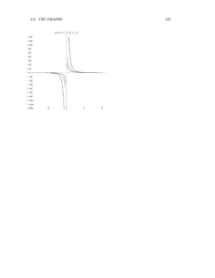
4.2. CRC GRAPHS 125

126 CHAPTER 4. CRC STANDARD CURVES AND SURFACES
Page 44 2.3.6
y =c
x2(a2 + b2)
a2x2y + x4y − c = 0
— p44-2.3.6.1-3 —
)clear all
f(x,a,c) == c/(x^2*(a^2+x^2))
lineColorDefault(red())
viewport1:=draw(f(x,0.2,0.02),x=-2..2,adaptive==true,unit==[1.0,1.0],_
title=="p44-2.3.6.1-3")
graph1:=getGraph(viewport1,1)
lineColorDefault(green())
viewport2:=draw(f(x,0.5,0.02),x=-2..2,adaptive==true,unit==[1.0,1.0])
graph2:=getGraph(viewport2,1)
lineColorDefault(blue())
viewport3:=draw(f(x,0.8,0.02),x=-2..2,adaptive==true,unit==[1.0,1.0])
graph3:=getGraph(viewport3,1)
putGraph(viewport1,graph2,2)
putGraph(viewport1,graph3,3)
units(viewport1,1,"on")
points(viewport1,1,"off")
points(viewport1,2,"off")
points(viewport1,3,"off")
makeViewport2D(viewport1)
———-

4.2. CRC GRAPHS 127

128 CHAPTER 4. CRC STANDARD CURVES AND SURFACES
Page 44 2.3.7
y = cx(a2 + x2)
y − a2cx− cx3 = 0
— p44-2.3.7.1-3 —
)clear all
f(x,a,c) == c*x*(a^2+x^2)
lineColorDefault(red())
viewport1:=draw(f(x,0.2,1.0),x=-2..2,adaptive==true,unit==[1.0,1.0],_
title=="p44-2.3.7.1-3")
graph1:=getGraph(viewport1,1)
lineColorDefault(green())
viewport2:=draw(f(x,0.5,1.0),x=-2..2,adaptive==true,unit==[1.0,1.0])
graph2:=getGraph(viewport2,1)
lineColorDefault(blue())
viewport3:=draw(f(x,0.8,1.0),x=-2..2,adaptive==true,unit==[1.0,1.0])
graph3:=getGraph(viewport3,1)
putGraph(viewport1,graph2,2)
putGraph(viewport1,graph3,3)
units(viewport1,1,"on")
points(viewport1,1,"off")
points(viewport1,2,"off")
points(viewport1,3,"off")
makeViewport2D(viewport1)
———-

4.2. CRC GRAPHS 129
Page 44 2.3.8
y = cx2(a2 + x2)
y − a2cx2 − cx4 = 0
— p44-2.3.8.1-3 —
)clear all
f(x,a,c) == c*x^2*(a^2+x^2)
lineColorDefault(red())
viewport1:=draw(f(x,0.2,1.0),x=-2..2,adaptive==true,unit==[1.0,1.0],_
title=="p44-2.3.8.1-3")
graph1:=getGraph(viewport1,1)
lineColorDefault(green())
viewport2:=draw(f(x,0.5,1.0),x=-2..2,adaptive==true,unit==[1.0,1.0])
graph2:=getGraph(viewport2,1)
lineColorDefault(blue())
viewport3:=draw(f(x,0.8,1.0),x=-2..2,adaptive==true,unit==[1.0,1.0])
graph3:=getGraph(viewport3,1)
putGraph(viewport1,graph2,2)
putGraph(viewport1,graph3,3)
units(viewport1,1,"on")
points(viewport1,1,"off")
points(viewport1,2,"off")
points(viewport1,3,"off")
makeViewport2D(viewport1)
———-

130 CHAPTER 4. CRC STANDARD CURVES AND SURFACES
4.2.4 Functions with a2 − x2 and xm
Page 46 2.4.1
y =c
(a2 − x2)
a2y − x2y − c = 0
— p46-2.4.1.1-3 —
)clear all
f(x,a,c) == c/(a^2-x^2)
lineColorDefault(red())
viewport1:=draw(f(x,0.2,0.03),x=-2..2,adaptive==true,unit==[1.0,1.0],_
title=="p46-2.4.1.1-3")
graph1:=getGraph(viewport1,1)
lineColorDefault(green())
viewport2:=draw(f(x,0.5,0.03),x=-2..2,adaptive==true,unit==[1.0,1.0])
graph2:=getGraph(viewport2,1)
lineColorDefault(blue())
viewport3:=draw(f(x,0.8,0.03),x=-2..2,adaptive==true,unit==[1.0,1.0])
graph3:=getGraph(viewport3,1)
putGraph(viewport1,graph2,2)
putGraph(viewport1,graph3,3)
units(viewport1,1,"on")
points(viewport1,1,"off")
points(viewport1,2,"off")
points(viewport1,3,"off")
makeViewport2D(viewport1)
———-

4.2. CRC GRAPHS 131

132 CHAPTER 4. CRC STANDARD CURVES AND SURFACES
Page 46 2.4.2
y =cx
(a2 − x2)
a2y − x2y − cx = 0
— p46-2.4.2.1-3 —
)clear all
f(x,a,c) == c*x/(a^2-x^2)
lineColorDefault(red())
viewport1:=draw(f(x,0.2,0.1),x=-2..2,adaptive==true,unit==[1.0,1.0],_
title=="p46-2.4.2.1-3")
graph1:=getGraph(viewport1,1)
lineColorDefault(green())
viewport2:=draw(f(x,0.5,0.1),x=-2..2,adaptive==true,unit==[1.0,1.0])
graph2:=getGraph(viewport2,1)
lineColorDefault(blue())
viewport3:=draw(f(x,0.8,0.1),x=-2..2,adaptive==true,unit==[1.0,1.0])
graph3:=getGraph(viewport3,1)
putGraph(viewport1,graph2,2)
putGraph(viewport1,graph3,3)
units(viewport1,1,"on")
points(viewport1,1,"off")
points(viewport1,2,"off")
points(viewport1,3,"off")
makeViewport2D(viewport1)
———-

4.2. CRC GRAPHS 133

134 CHAPTER 4. CRC STANDARD CURVES AND SURFACES
Page 46 2.4.3
y =cx2
(a2 − x2)
a2y − x2y − cx2 = 0
— p46-2.4.3.1-3 —
)clear all
f(x,a,c) == c*x^2/(a^2-x^2)
lineColorDefault(red())
viewport1:=draw(f(x,0.2,0.2),x=-2..2,adaptive==true,unit==[1.0,1.0],_
title=="p46-2.4.3.1-3")
graph1:=getGraph(viewport1,1)
lineColorDefault(green())
viewport2:=draw(f(x,0.5,0.2),x=-2..2,adaptive==true,unit==[1.0,1.0])
graph2:=getGraph(viewport2,1)
lineColorDefault(blue())
viewport3:=draw(f(x,0.8,0.2),x=-2..2,adaptive==true,unit==[1.0,1.0])
graph3:=getGraph(viewport3,1)
putGraph(viewport1,graph2,2)
putGraph(viewport1,graph3,3)
units(viewport1,1,"on")
points(viewport1,1,"off")
points(viewport1,2,"off")
points(viewport1,3,"off")
makeViewport2D(viewport1)
———-

4.2. CRC GRAPHS 135

136 CHAPTER 4. CRC STANDARD CURVES AND SURFACES
Page 46 2.4.4
y =cx3
(a2 − x2)
a2y − x2y − cx3 = 0
— p46-2.4.4.1-3 —
)clear all
f(x,a,c) == c*x^3/(a^2-x^2)
lineColorDefault(red())
viewport1:=draw(f(x,0.2,0.2),x=-2..2,adaptive==true,unit==[1.0,1.0],_
title=="p46-2.4.4.1-3")
graph1:=getGraph(viewport1,1)
lineColorDefault(green())
viewport2:=draw(f(x,0.5,0.2),x=-2..2,adaptive==true,unit==[1.0,1.0])
graph2:=getGraph(viewport2,1)
lineColorDefault(blue())
viewport3:=draw(f(x,0.8,0.2),x=-2..2,adaptive==true,unit==[1.0,1.0])
graph3:=getGraph(viewport3,1)
putGraph(viewport1,graph2,2)
putGraph(viewport1,graph3,3)
units(viewport1,1,"on")
points(viewport1,1,"off")
points(viewport1,2,"off")
points(viewport1,3,"off")
makeViewport2D(viewport1)
———-

4.2. CRC GRAPHS 137

138 CHAPTER 4. CRC STANDARD CURVES AND SURFACES
Page 48 2.4.5
y =c
x(a2 − x2)
a2xy − x3y − c = 0
— p48-2.4.5.1-3 —
)clear all
f(x,a,c) == c/(x*(a^2-x^2))
lineColorDefault(red())
viewport1:=draw(f(x,0.2,0.001),x=-2..2,adaptive==true,unit==[1.0,1.0],_
title=="p48-2.4.5.1-3")
graph1:=getGraph(viewport1,1)
lineColorDefault(green())
viewport2:=draw(f(x,0.5,0.001),x=-2..2,adaptive==true,unit==[1.0,1.0])
graph2:=getGraph(viewport2,1)
lineColorDefault(blue())
viewport3:=draw(f(x,0.8,0.001),x=-2..2,adaptive==true,unit==[1.0,1.0])
graph3:=getGraph(viewport3,1)
putGraph(viewport1,graph2,2)
putGraph(viewport1,graph3,3)
units(viewport1,1,"on")
points(viewport1,1,"off")
points(viewport1,2,"off")
points(viewport1,3,"off")
makeViewport2D(viewport1)
———-

4.2. CRC GRAPHS 139

140 CHAPTER 4. CRC STANDARD CURVES AND SURFACES
Page 48 2.4.6
y =c
x2(a2 − x2)
a2x2y − x4y − c = 0
— p48-2.4.6.1-3 —
)clear all
f(x,a,c) == c/(x^2*(a^2-x^2))
lineColorDefault(red())
viewport1:=draw(f(x,0.2,0.0003),x=-2..2,adaptive==true,unit==[1.0,1.0],_
title=="p48-2.4.6.1-3")
graph1:=getGraph(viewport1,1)
lineColorDefault(green())
viewport2:=draw(f(x,0.5,0.0003),x=-2..2,adaptive==true,unit==[1.0,1.0])
graph2:=getGraph(viewport2,1)
lineColorDefault(blue())
viewport3:=draw(f(x,0.8,0.0003),x=-2..2,adaptive==true,unit==[1.0,1.0])
graph3:=getGraph(viewport3,1)
putGraph(viewport1,graph2,2)
putGraph(viewport1,graph3,3)
units(viewport1,1,"on")
points(viewport1,1,"off")
points(viewport1,2,"off")
points(viewport1,3,"off")
makeViewport2D(viewport1)
———-

4.2. CRC GRAPHS 141

142 CHAPTER 4. CRC STANDARD CURVES AND SURFACES
Page 48 2.4.7
y = cx(a2 − x2)
y − a2cx+ cx3 = 0
— p48-2.4.7.1-3 —
)clear all
f(x,a,c) == c*x*(a^2-x^2)
lineColorDefault(red())
viewport1:=draw(f(x,0.2,1.0),x=-2..2,adaptive==true,unit==[1.0,1.0],_
title=="p48-2.4.7.1-3")
graph1:=getGraph(viewport1,1)
lineColorDefault(green())
viewport2:=draw(f(x,0.5,1.0),x=-2..2,adaptive==true,unit==[1.0,1.0])
graph2:=getGraph(viewport2,1)
lineColorDefault(blue())
viewport3:=draw(f(x,0.8,1.0),x=-2..2,adaptive==true,unit==[1.0,1.0])
graph3:=getGraph(viewport3,1)
putGraph(viewport1,graph2,2)
putGraph(viewport1,graph3,3)
units(viewport1,1,"on")
points(viewport1,1,"off")
points(viewport1,2,"off")
points(viewport1,3,"off")
makeViewport2D(viewport1)
———-
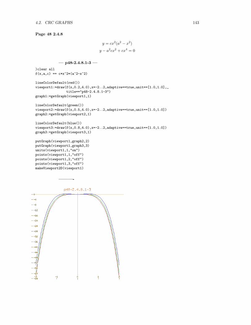
4.2. CRC GRAPHS 143
Page 48 2.4.8
y = cx2(a2 − x2)
y − a2cx2 + cx4 = 0
— p48-2.4.8.1-3 —
)clear all
f(x,a,c) == c*x^2*(a^2-x^2)
lineColorDefault(red())
viewport1:=draw(f(x,0.2,4.0),x=-2..2,adaptive==true,unit==[1.0,1.0],_
title=="p48-2.4.8.1-3")
graph1:=getGraph(viewport1,1)
lineColorDefault(green())
viewport2:=draw(f(x,0.5,4.0),x=-2..2,adaptive==true,unit==[1.0,1.0])
graph2:=getGraph(viewport2,1)
lineColorDefault(blue())
viewport3:=draw(f(x,0.8,4.0),x=-2..2,adaptive==true,unit==[1.0,1.0])
graph3:=getGraph(viewport3,1)
putGraph(viewport1,graph2,2)
putGraph(viewport1,graph3,3)
units(viewport1,1,"on")
points(viewport1,1,"off")
points(viewport1,2,"off")
points(viewport1,3,"off")
makeViewport2D(viewport1)
———-
144 CHAPTER 4. CRC STANDARD CURVES AND SURFACES
4.2.5 Functions with a3 + x3 and xm
Page 50 2.5.1
y =c
(a3 + x3)
a3y + x3y − c = 0
— p50-2.5.1.1-3 —
)clear all
f(x,a,c) == c/(a^3+x^3)
lineColorDefault(red())
viewport1:=draw(f(x,0.2,0.01),x=-2..2,adaptive==true,unit==[1.0,1.0],_
title=="p50-2.5.1.1-3")
graph1:=getGraph(viewport1,1)
lineColorDefault(green())
viewport2:=draw(f(x,0.3,0.01),x=-2..2,adaptive==true,unit==[1.0,1.0])
graph2:=getGraph(viewport2,1)
lineColorDefault(blue())
viewport3:=draw(f(x,0.4,0.01),x=-2..2,adaptive==true,unit==[1.0,1.0])
graph3:=getGraph(viewport3,1)
putGraph(viewport1,graph2,2)
putGraph(viewport1,graph3,3)
units(viewport1,1,"on")
points(viewport1,1,"off")
points(viewport1,2,"off")
points(viewport1,3,"off")
makeViewport2D(viewport1)
———-

4.2. CRC GRAPHS 145

146 CHAPTER 4. CRC STANDARD CURVES AND SURFACES
Page 50 2.5.2
y =cx
(a3 + x3)
a3y + x3y − cx = 0
— p50-2.5.2.1-3 —
)clear all
f(x,a,c) == c*x/(a^3+x^3)
lineColorDefault(red())
viewport1:=draw(f(x,0.1,0.01),x=-2..2,adaptive==true,unit==[1.0,1.0],_
title=="p50-2.5.2.1-3")
graph1:=getGraph(viewport1,1)
lineColorDefault(green())
viewport2:=draw(f(x,0.3,0.01),x=-2..2,adaptive==true,unit==[1.0,1.0])
graph2:=getGraph(viewport2,1)
lineColorDefault(blue())
viewport3:=draw(f(x,0.5,0.01),x=-2..2,adaptive==true,unit==[1.0,1.0])
graph3:=getGraph(viewport3,1)
putGraph(viewport1,graph2,2)
putGraph(viewport1,graph3,3)
units(viewport1,1,"on")
points(viewport1,1,"off")
points(viewport1,2,"off")
points(viewport1,3,"off")
makeViewport2D(viewport1)
———-

4.2. CRC GRAPHS 147

148 CHAPTER 4. CRC STANDARD CURVES AND SURFACES
Page 50 2.5.3
y =cx2
(a3 + x3)
a3y + x3y − cx2 = 0
— p50-2.5.3.1-3 —
)clear all
f(x,a,c) == c*x^2/(a^3+x^3)
lineColorDefault(red())
viewport1:=draw(f(x,0.1,0.01),x=-2..2,adaptive==true,unit==[1.0,1.0],_
title=="p50-2.5.3.1-3")
graph1:=getGraph(viewport1,1)
lineColorDefault(green())
viewport2:=draw(f(x,0.3,0.01),x=-2..2,adaptive==true,unit==[1.0,1.0])
graph2:=getGraph(viewport2,1)
lineColorDefault(blue())
viewport3:=draw(f(x,0.5,0.01),x=-2..2,adaptive==true,unit==[1.0,1.0])
graph3:=getGraph(viewport3,1)
putGraph(viewport1,graph2,2)
putGraph(viewport1,graph3,3)
units(viewport1,1,"on")
points(viewport1,1,"off")
points(viewport1,2,"off")
points(viewport1,3,"off")
makeViewport2D(viewport1)
———-

4.2. CRC GRAPHS 149

150 CHAPTER 4. CRC STANDARD CURVES AND SURFACES
Page 50 2.5.4
y =cx3
(a3 + x3)
a3y + x3y − cx3 = 0
— p50-2.5.4.1-3 —
)clear all
f(x,a,c) == c*x^3/(a^3+x^3)
lineColorDefault(red())
viewport1:=draw(f(x,0.1,0.02),x=-2..2,adaptive==true,unit==[1.0,1.0],_
title=="p50-2.5.4.1-3")
graph1:=getGraph(viewport1,1)
lineColorDefault(green())
viewport2:=draw(f(x,0.3,0.02),x=-2..2,adaptive==true,unit==[1.0,1.0])
graph2:=getGraph(viewport2,1)
lineColorDefault(blue())
viewport3:=draw(f(x,0.5,0.02),x=-2..2,adaptive==true,unit==[1.0,1.0])
graph3:=getGraph(viewport3,1)
putGraph(viewport1,graph2,2)
putGraph(viewport1,graph3,3)
units(viewport1,1,"on")
points(viewport1,1,"off")
points(viewport1,2,"off")
points(viewport1,3,"off")
makeViewport2D(viewport1)
———-

4.2. CRC GRAPHS 151

152 CHAPTER 4. CRC STANDARD CURVES AND SURFACES
Page 50 2.5.5
y =c
x(a3 + x3)
a3xy + x4y − c = 0
— p50-2.5.5.1-3 —
)clear all
f(x,a,c) == c/(x*(a^3+x^3))
lineColorDefault(red())
viewport1:=draw(f(x,0.5,0.01),x=-2..2,adaptive==true,unit==[1.0,1.0],_
title=="p50-2.5.5.1-3")
graph1:=getGraph(viewport1,1)
lineColorDefault(green())
viewport2:=draw(f(x,0.7,0.01),x=-2..2,adaptive==true,unit==[1.0,1.0])
graph2:=getGraph(viewport2,1)
lineColorDefault(blue())
viewport3:=draw(f(x,0.9,0.01),x=-2..2,adaptive==true,unit==[1.0,1.0])
graph3:=getGraph(viewport3,1)
putGraph(viewport1,graph2,2)
putGraph(viewport1,graph3,3)
units(viewport1,1,"on")
points(viewport1,1,"off")
points(viewport1,2,"off")
points(viewport1,3,"off")
makeViewport2D(viewport1)
———-

4.2. CRC GRAPHS 153

154 CHAPTER 4. CRC STANDARD CURVES AND SURFACES
Page 50 2.5.6
y = cx(a3 + x3)
y − a3cx− cx4 = 0
— p50-2.5.6.1-3 —
)clear all
f(x,a,c) == c*x*(a^3+x^3)
lineColorDefault(red())
viewport1:=draw(f(x,0.5,1.0),x=-2..2,adaptive==true,unit==[1.0,1.0],_
title=="p50-2.5.6.1-3")
graph1:=getGraph(viewport1,1)
lineColorDefault(green())
viewport2:=draw(f(x,0.7,1.0),x=-2..2,adaptive==true,unit==[1.0,1.0])
graph2:=getGraph(viewport2,1)
lineColorDefault(blue())
viewport3:=draw(f(x,0.9,1.0),x=-2..2,adaptive==true,unit==[1.0,1.0])
graph3:=getGraph(viewport3,1)
putGraph(viewport1,graph2,2)
putGraph(viewport1,graph3,3)
units(viewport1,1,"on")
points(viewport1,1,"off")
points(viewport1,2,"off")
points(viewport1,3,"off")
makeViewport2D(viewport1)
———-

4.2. CRC GRAPHS 155
4.2.6 Functions with a3 − x3 and xm
Page 52 2.6.1
y =c
(a3 − x3)
a3y − x3y − c = 0
— p52-2.6.1.1-3 —
)clear all
f(x,a,c) == c/(a^3-x^3)
lineColorDefault(red())
viewport1:=draw(f(x,0.2,0.01),x=-2..2,adaptive==true,unit==[1.0,1.0],_
title=="p52-2.6.1.1-3")
graph1:=getGraph(viewport1,1)
lineColorDefault(green())
viewport2:=draw(f(x,0.3,0.01),x=-2..2,adaptive==true,unit==[1.0,1.0])
graph2:=getGraph(viewport2,1)
lineColorDefault(blue())
viewport3:=draw(f(x,0.4,0.01),x=-2..2,adaptive==true,unit==[1.0,1.0])
graph3:=getGraph(viewport3,1)
putGraph(viewport1,graph2,2)
putGraph(viewport1,graph3,3)
units(viewport1,1,"on")
points(viewport1,1,"off")
points(viewport1,2,"off")
points(viewport1,3,"off")
makeViewport2D(viewport1)
———-

156 CHAPTER 4. CRC STANDARD CURVES AND SURFACES

4.2. CRC GRAPHS 157
Page 52 2.6.2
y =cx
(a3 − x3)
a3y − x3y − cx = 0
— p52-2.6.2.1-3 —
)clear all
f(x,a,c) == c*x/(a^3-x^3)
lineColorDefault(red())
viewport1:=draw(f(x,0.1,0.01),x=-2..2,adaptive==true,unit==[1.0,1.0],_
title=="p52-2.6.2.1-3")
graph1:=getGraph(viewport1,1)
lineColorDefault(green())
viewport2:=draw(f(x,0.3,0.01),x=-2..2,adaptive==true,unit==[1.0,1.0])
graph2:=getGraph(viewport2,1)
lineColorDefault(blue())
viewport3:=draw(f(x,0.5,0.01),x=-2..2,adaptive==true,unit==[1.0,1.0])
graph3:=getGraph(viewport3,1)
putGraph(viewport1,graph2,2)
putGraph(viewport1,graph3,3)
units(viewport1,1,"on")
points(viewport1,1,"off")
points(viewport1,2,"off")
points(viewport1,3,"off")
makeViewport2D(viewport1)
———-

158 CHAPTER 4. CRC STANDARD CURVES AND SURFACES
4.2. CRC GRAPHS 159
Page 52 2.6.3
y =cx2
(a3 − x3)
a3y − x3y − cx2 = 0
— p52-2.6.3.1-3 —
)clear all
f(x,a,c) == c*x^2/(a^3-x^3)
lineColorDefault(red())
viewport1:=draw(f(x,0.1,0.1),x=-2..2,adaptive==true,unit==[1.0,1.0],_
title=="p52-2.6.3.1-3")
graph1:=getGraph(viewport1,1)
lineColorDefault(green())
viewport2:=draw(f(x,0.3,0.1),x=-2..2,adaptive==true,unit==[1.0,1.0])
graph2:=getGraph(viewport2,1)
lineColorDefault(blue())
viewport3:=draw(f(x,0.5,0.1),x=-2..2,adaptive==true,unit==[1.0,1.0])
graph3:=getGraph(viewport3,1)
putGraph(viewport1,graph2,2)
putGraph(viewport1,graph3,3)
units(viewport1,1,"on")
points(viewport1,1,"off")
points(viewport1,2,"off")
points(viewport1,3,"off")
makeViewport2D(viewport1)
———-

160 CHAPTER 4. CRC STANDARD CURVES AND SURFACES

4.2. CRC GRAPHS 161
Page 52 2.6.4
y =cx3
(a3 − x3)
a3y − x3y − cx3 = 0
— p52-2.6.4.1-3 —
)clear all
f(x,a,c) == c*x^3/(a^3-x^3)
lineColorDefault(red())
viewport1:=draw(f(x,0.1,0.2),x=-2..2,adaptive==true,unit==[1.0,1.0],_
title=="p52-2.6.4.1-3")
graph1:=getGraph(viewport1,1)
lineColorDefault(green())
viewport2:=draw(f(x,0.3,0.2),x=-2..2,adaptive==true,unit==[1.0,1.0])
graph2:=getGraph(viewport2,1)
lineColorDefault(blue())
viewport3:=draw(f(x,0.5,0.2),x=-2..2,adaptive==true,unit==[1.0,1.0])
graph3:=getGraph(viewport3,1)
putGraph(viewport1,graph2,2)
putGraph(viewport1,graph3,3)
units(viewport1,1,"on")
points(viewport1,1,"off")
points(viewport1,2,"off")
points(viewport1,3,"off")
makeViewport2D(viewport1)
———-

162 CHAPTER 4. CRC STANDARD CURVES AND SURFACES

4.2. CRC GRAPHS 163
Page 52 2.6.5
y =c
x(a3 − x3)
a3xy − x4y − c = 0
— p52-2.6.5.1-3 —
)clear all
f(x,a,c) == c/(x*(a^3-x^3))
lineColorDefault(red())
viewport1:=draw(f(x,0.5,0.01),x=-2..2,adaptive==true,unit==[1.0,1.0],_
title=="p52-2.6.5.1-3")
graph1:=getGraph(viewport1,1)
lineColorDefault(green())
viewport2:=draw(f(x,0.7,0.01),x=-2..2,adaptive==true,unit==[1.0,1.0])
graph2:=getGraph(viewport2,1)
lineColorDefault(blue())
viewport3:=draw(f(x,0.9,0.01),x=-2..2,adaptive==true,unit==[1.0,1.0])
graph3:=getGraph(viewport3,1)
putGraph(viewport1,graph2,2)
putGraph(viewport1,graph3,3)
units(viewport1,1,"on")
points(viewport1,1,"off")
points(viewport1,2,"off")
points(viewport1,3,"off")
makeViewport2D(viewport1)
———-

164 CHAPTER 4. CRC STANDARD CURVES AND SURFACES

4.2. CRC GRAPHS 165
Page 52 2.6.6
y = cx(a3 − x3)
y − a3cx+ cx4 = 0
— p52-2.6.6.1-3 —
)clear all
f(x,a,c) == c*x*(a^3-x^3)
lineColorDefault(red())
viewport1:=draw(f(x,0.5,1.0),x=-2..2,adaptive==true,unit==[1.0,1.0],_
title=="p52-2.6.6.1-3")
graph1:=getGraph(viewport1,1)
lineColorDefault(green())
viewport2:=draw(f(x,0.7,1.0),x=-2..2,adaptive==true,unit==[1.0,1.0])
graph2:=getGraph(viewport2,1)
lineColorDefault(blue())
viewport3:=draw(f(x,0.9,1.0),x=-2..2,adaptive==true,unit==[1.0,1.0])
graph3:=getGraph(viewport3,1)
putGraph(viewport1,graph2,2)
putGraph(viewport1,graph3,3)
units(viewport1,1,"on")
points(viewport1,1,"off")
points(viewport1,2,"off")
points(viewport1,3,"off")
makeViewport2D(viewport1)
———-
166 CHAPTER 4. CRC STANDARD CURVES AND SURFACES
4.2.7 Functions with a4 + x4 and xm
Page 54 2.7.1
y =c
(a4 + x4)
a4y + x4y − c = 0
— p54-2.7.1.1-3 —
)clear all
f(x,a,c) == c/(a^4+x^4)
lineColorDefault(red())
viewport1:=draw(f(x,0.3,0.007),x=-2..2,adaptive==true,unit==[1.0,1.0],_
title=="p54-2.7.1.1-3")
graph1:=getGraph(viewport1,1)
lineColorDefault(green())
viewport2:=draw(f(x,0.4,0.007),x=-2..2,adaptive==true,unit==[1.0,1.0])
graph2:=getGraph(viewport2,1)
lineColorDefault(blue())
viewport3:=draw(f(x,0.5,0.007),x=-2..2,adaptive==true,unit==[1.0,1.0])
graph3:=getGraph(viewport3,1)
putGraph(viewport1,graph2,2)
putGraph(viewport1,graph3,3)
units(viewport1,1,"on")
points(viewport1,1,"off")
points(viewport1,2,"off")
points(viewport1,3,"off")
makeViewport2D(viewport1)
———-

4.2. CRC GRAPHS 167

168 CHAPTER 4. CRC STANDARD CURVES AND SURFACES
Page 54 2.7.2
y =cx
(a4 + x4)
a4y + x4y − cx = 0
— p54-2.7.2.1-3 —
)clear all
f(x,a,c) == c*x/(a^4+x^4)
lineColorDefault(red())
viewport1:=draw(f(x,0.2,0.01),x=-2..2,adaptive==true,unit==[1.0,1.0],_
title=="p54-2.7.2.1-3")
graph1:=getGraph(viewport1,1)
lineColorDefault(green())
viewport2:=draw(f(x,0.3,0.01),x=-2..2,adaptive==true,unit==[1.0,1.0])
graph2:=getGraph(viewport2,1)
lineColorDefault(blue())
viewport3:=draw(f(x,0.4,0.01),x=-2..2,adaptive==true,unit==[1.0,1.0])
graph3:=getGraph(viewport3,1)
putGraph(viewport1,graph2,2)
putGraph(viewport1,graph3,3)
units(viewport1,1,"on")
points(viewport1,1,"off")
points(viewport1,2,"off")
points(viewport1,3,"off")
makeViewport2D(viewport1)
———-

4.2. CRC GRAPHS 169

170 CHAPTER 4. CRC STANDARD CURVES AND SURFACES
Page 54 2.7.3
y =cx2
(a4 + x4)
a4y + x4y − cx2 = 0
— p54-2.7.3.1-3 —
)clear all
f(x,a,c) == c*x^2/(a^4+x^4)
lineColorDefault(red())
viewport1:=draw(f(x,0.3,0.15),x=-2..2,adaptive==true,unit==[1.0,1.0],_
title=="p54-2.7.3.1-3")
graph1:=getGraph(viewport1,1)
lineColorDefault(green())
viewport2:=draw(f(x,0.4,0.15),x=-2..2,adaptive==true,unit==[1.0,1.0])
graph2:=getGraph(viewport2,1)
lineColorDefault(blue())
viewport3:=draw(f(x,0.5,0.15),x=-2..2,adaptive==true,unit==[1.0,1.0])
graph3:=getGraph(viewport3,1)
putGraph(viewport1,graph2,2)
putGraph(viewport1,graph3,3)
units(viewport1,1,"on")
points(viewport1,1,"off")
points(viewport1,2,"off")
points(viewport1,3,"off")
makeViewport2D(viewport1)
———-

4.2. CRC GRAPHS 171

172 CHAPTER 4. CRC STANDARD CURVES AND SURFACES
Page 54 2.7.4
y =cx3
(a4 + x4)
a4y + x4y − cx3 = 0
— p54-2.7.4.1-3 —
)clear all
f(x,a,c) == c*x^3/(a^4+x^4)
lineColorDefault(red())
viewport1:=draw(f(x,0.2,0.25),x=-2..2,adaptive==true,unit==[1.0,1.0],_
title=="p54-2.7.4.1-3")
graph1:=getGraph(viewport1,1)
lineColorDefault(green())
viewport2:=draw(f(x,0.4,0.25),x=-2..2,adaptive==true,unit==[1.0,1.0])
graph2:=getGraph(viewport2,1)
lineColorDefault(blue())
viewport3:=draw(f(x,0.6,0.25),x=-2..2,adaptive==true,unit==[1.0,1.0])
graph3:=getGraph(viewport3,1)
putGraph(viewport1,graph2,2)
putGraph(viewport1,graph3,3)
units(viewport1,1,"on")
points(viewport1,1,"off")
points(viewport1,2,"off")
points(viewport1,3,"off")
makeViewport2D(viewport1)
———-

4.2. CRC GRAPHS 173

174 CHAPTER 4. CRC STANDARD CURVES AND SURFACES
Page 54 2.7.5
y =cx4
(a4 + x4)
a4y + x4y − cx4 = 0
— p54-2.7.5.1-3 —
)clear all
f(x,a,c) == c*x^4/(a^4+x^4)
lineColorDefault(red())
viewport1:=draw(f(x,0.2,1.0),x=-2..2,adaptive==true,unit==[1.0,1.0],_
title=="p54-2.7.5.1-3")
graph1:=getGraph(viewport1,1)
lineColorDefault(green())
viewport2:=draw(f(x,0.5,1.0),x=-2..2,adaptive==true,unit==[1.0,1.0])
graph2:=getGraph(viewport2,1)
lineColorDefault(blue())
viewport3:=draw(f(x,0.8,1.0),x=-2..2,adaptive==true,unit==[1.0,1.0])
graph3:=getGraph(viewport3,1)
putGraph(viewport1,graph2,2)
putGraph(viewport1,graph3,3)
units(viewport1,1,"on")
points(viewport1,1,"off")
points(viewport1,2,"off")
points(viewport1,3,"off")
makeViewport2D(viewport1)
———-

4.2. CRC GRAPHS 175

176 CHAPTER 4. CRC STANDARD CURVES AND SURFACES
Page 54 2.7.6
y = cx(a4 + x4)
y − a4cx− cx5 = 0
— p54-2.7.6.1-3 —
)clear all
f(x,a,c) == c*x*(a^4+x^4)
lineColorDefault(red())
viewport1:=draw(f(x,0.5,0.5),x=-2..2,adaptive==true,unit==[1.0,1.0],_
title=="p54-2.7.6.1-3")
graph1:=getGraph(viewport1,1)
lineColorDefault(green())
viewport2:=draw(f(x,1.0,0.5),x=-2..2,adaptive==true,unit==[1.0,1.0])
graph2:=getGraph(viewport2,1)
lineColorDefault(blue())
viewport3:=draw(f(x,1.2,0.5),x=-2..2,adaptive==true,unit==[1.0,1.0])
graph3:=getGraph(viewport3,1)
putGraph(viewport1,graph2,2)
putGraph(viewport1,graph3,3)
units(viewport1,1,"on")
points(viewport1,1,"off")
points(viewport1,2,"off")
points(viewport1,3,"off")
makeViewport2D(viewport1)
———-

4.2. CRC GRAPHS 177
4.2.8 Functions with a4 − x4 and xm
Page 56 2.8.1
y =c
(a4 − x4)
a4y − x4y − c = 0
— p56-2.8.1.1-3 —
)clear all
f(x,a,c) == c/(a^4-x^4)
lineColorDefault(red())
viewport1:=draw(f(x,0.4,0.01),x=-2..2,adaptive==true,unit==[1.0,1.0],_
title=="p56-2.8.1.1-3")
graph1:=getGraph(viewport1,1)
lineColorDefault(green())
viewport2:=draw(f(x,0.6,0.01),x=-2..2,adaptive==true,unit==[1.0,1.0])
graph2:=getGraph(viewport2,1)
lineColorDefault(blue())
viewport3:=draw(f(x,0.8,0.01),x=-2..2,adaptive==true,unit==[1.0,1.0])
graph3:=getGraph(viewport3,1)
putGraph(viewport1,graph2,2)
putGraph(viewport1,graph3,3)
units(viewport1,1,"on")
points(viewport1,1,"off")
points(viewport1,2,"off")
points(viewport1,3,"off")
makeViewport2D(viewport1)
———-

178 CHAPTER 4. CRC STANDARD CURVES AND SURFACES

4.2. CRC GRAPHS 179
Page 56 2.8.2
y =cx
(a4 − x4)
a4y − x4y − cx = 0
— p56-2.8.2.1-3 —
)clear all
f(x,a,c) == c*x/(a^4-x^4)
lineColorDefault(red())
viewport1:=draw(f(x,0.2,0.01),x=-2..2,adaptive==true,unit==[1.0,1.0],_
title=="p56-2.8.2.1-3")
graph1:=getGraph(viewport1,1)
lineColorDefault(green())
viewport2:=draw(f(x,0.4,0.01),x=-2..2,adaptive==true,unit==[1.0,1.0])
graph2:=getGraph(viewport2,1)
lineColorDefault(blue())
viewport3:=draw(f(x,0.6,0.01),x=-2..2,adaptive==true,unit==[1.0,1.0])
graph3:=getGraph(viewport3,1)
putGraph(viewport1,graph2,2)
putGraph(viewport1,graph3,3)
units(viewport1,1,"on")
points(viewport1,1,"off")
points(viewport1,2,"off")
points(viewport1,3,"off")
makeViewport2D(viewport1)
———-
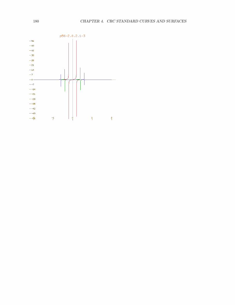
180 CHAPTER 4. CRC STANDARD CURVES AND SURFACES

4.2. CRC GRAPHS 181
Page 56 2.8.3
y =cx2
(a4 − x4)
a4y − x4y − cx2 = 0
— p56-2.8.3.1-3 —
)clear all
f(x,a,c) == c*x^2/(a^4-x^4)
lineColorDefault(red())
viewport1:=draw(f(x,0.2,0.1),x=-2..2,adaptive==true,unit==[1.0,1.0],_
title=="p56-2.8.3.1-3")
graph1:=getGraph(viewport1,1)
lineColorDefault(green())
viewport2:=draw(f(x,0.4,0.1),x=-2..2,adaptive==true,unit==[1.0,1.0])
graph2:=getGraph(viewport2,1)
lineColorDefault(blue())
viewport3:=draw(f(x,0.6,0.1),x=-2..2,adaptive==true,unit==[1.0,1.0])
graph3:=getGraph(viewport3,1)
putGraph(viewport1,graph2,2)
putGraph(viewport1,graph3,3)
units(viewport1,1,"on")
points(viewport1,1,"off")
points(viewport1,2,"off")
points(viewport1,3,"off")
makeViewport2D(viewport1)
———-

182 CHAPTER 4. CRC STANDARD CURVES AND SURFACES

4.2. CRC GRAPHS 183
Page 56 2.8.4
y =cx3
(a4 − x4)
a4y − x4y − cx3 = 0
— p56-2.8.4.1-3 —
)clear all
f(x,a,c) == c*x^3/(a^4-x^4)
lineColorDefault(red())
viewport1:=draw(f(x,0.2,0.1),x=-2..2,adaptive==true,unit==[1.0,1.0],_
title=="p56-2.8.4.1-3")
graph1:=getGraph(viewport1,1)
lineColorDefault(green())
viewport2:=draw(f(x,0.4,0.1),x=-2..2,adaptive==true,unit==[1.0,1.0])
graph2:=getGraph(viewport2,1)
lineColorDefault(blue())
viewport3:=draw(f(x,0.6,0.1),x=-2..2,adaptive==true,unit==[1.0,1.0])
graph3:=getGraph(viewport3,1)
putGraph(viewport1,graph2,2)
putGraph(viewport1,graph3,3)
units(viewport1,1,"on")
points(viewport1,1,"off")
points(viewport1,2,"off")
points(viewport1,3,"off")
makeViewport2D(viewport1)
———-

184 CHAPTER 4. CRC STANDARD CURVES AND SURFACES

4.2. CRC GRAPHS 185
Page 56 2.8.5
y =cx4
(a4 − x4)
a4y − x4y − cx4 = 0
— p56-2.8.5.1-3 —
)clear all
f(x,a,c) == c*x^4/(a^4-x^4)
lineColorDefault(red())
viewport1:=draw(f(x,0.2,0.1),x=-2..2,adaptive==true,unit==[1.0,1.0],_
title=="p56-2.8.5.1-3")
graph1:=getGraph(viewport1,1)
lineColorDefault(green())
viewport2:=draw(f(x,0.5,0.1),x=-2..2,adaptive==true,unit==[1.0,1.0])
graph2:=getGraph(viewport2,1)
lineColorDefault(blue())
viewport3:=draw(f(x,0.8,0.1),x=-2..2,adaptive==true,unit==[1.0,1.0])
graph3:=getGraph(viewport3,1)
putGraph(viewport1,graph2,2)
putGraph(viewport1,graph3,3)
units(viewport1,1,"on")
points(viewport1,1,"off")
points(viewport1,2,"off")
points(viewport1,3,"off")
makeViewport2D(viewport1)
———-

186 CHAPTER 4. CRC STANDARD CURVES AND SURFACES

4.2. CRC GRAPHS 187
Page 56 2.8.6
y = cx(a4 − x4)
y − a4cx+ cx5 = 0
— p56-2.8.6.1-3 —
)clear all
f(x,a,c) == c*x*(a^4-x^4)
lineColorDefault(red())
viewport1:=draw(f(x,0.4,1.0),x=-2..2,adaptive==true,unit==[1.0,1.0],_
title=="p56-2.8.6.1-3")
graph1:=getGraph(viewport1,1)
lineColorDefault(green())
viewport2:=draw(f(x,0.8,1.0),x=-2..2,adaptive==true,unit==[1.0,1.0])
graph2:=getGraph(viewport2,1)
lineColorDefault(blue())
viewport3:=draw(f(x,1.0,1.0),x=-2..2,adaptive==true,unit==[1.0,1.0])
graph3:=getGraph(viewport3,1)
putGraph(viewport1,graph2,2)
putGraph(viewport1,graph3,3)
units(viewport1,1,"on")
points(viewport1,1,"off")
points(viewport1,2,"off")
points(viewport1,3,"off")
makeViewport2D(viewport1)
———-

188 CHAPTER 4. CRC STANDARD CURVES AND SURFACES
4.2.9 Functions with (a+ bx)1/2 and xm
Page 58 2.9.1
Parabolay = c(a+ bx)1/2
y2 − bc2x− ac2 = 0
— p58-2.9.1.1-3 —
)clear all
f1(x,y) == y^2 - x/8 - 1/2
lineColorDefault(red())
viewport1:=draw(f1(x,y)=0,x,y,range==[-4.0..4.0,-4.0..4.0],adaptive==true,_
unit==[1.0,1.0],title=="p58-2.9.1.1-3")
graph1:=getGraph(viewport1,1)
f2(x,y) == y^2 - x - 1/2
lineColorDefault(green())
viewport2:=draw(f2(x,y)=0,x,y,range==[-4.0..4.0,-4.0..4.0],adaptive==true,_
unit==[1.0,1.0])
graph2:=getGraph(viewport2,1)
f3(x,y) == y^2 - 2*x - 1/2
lineColorDefault(blue())
viewport3:=draw(f3(x,y)=0,x,y,range==[-4.0..4.0,-4.0..4.0],adaptive==true,_
unit==[1.0,1.0])
graph3:=getGraph(viewport3,1)
putGraph(viewport1,graph2,2)
putGraph(viewport1,graph3,3)
units(viewport1,1,"on")
points(viewport1,1,"off")
points(viewport1,2,"off")
points(viewport1,3,"off")
makeViewport2D(viewport1)
———-

4.2. CRC GRAPHS 189

190 CHAPTER 4. CRC STANDARD CURVES AND SURFACES
Page 58 2.9.2
Trisectrix of Catalan... fails ”singular pts in region of sketch”
y = cx(a+ bx)1/2
y2 − bc2x3 − ac2x2 = 0
— p58-2.9.2.1-3 —
)clear all
f1(x,y) == y^2 - x^3/2 - x^2/2
lineColorDefault(red())
viewport1:=draw(f1(x,y)=0,x,y,range==[-4.0..4.0,-4.0..4.0],adaptive==true,_
unit==[1.0,1.0],title=="p58-2.9.2.1-3")
graph1:=getGraph(viewport1,1)
f2(x,y) == y^2 - x^3 - x^2/2
lineColorDefault(green())
viewport2:=draw(f2(x,y)=0,x,y,range==[-4.0..4.0,-4.0..4.0],adaptive==true,_
unit==[1.0,1.0])
graph2:=getGraph(viewport2,1)
f3(x,y) == y^2 - 2*x^3 - x^2/2
lineColorDefault(blue())
viewport3:=draw(f3(x,y)=0,x,y,range==[-4.0..4.0,-4.0..4.0],adaptive==true,_
unit==[1.0,1.0])
graph3:=getGraph(viewport3,1)
putGraph(viewport1,graph2,2)
putGraph(viewport1,graph3,3)
units(viewport1,1,"on")
points(viewport1,1,"off")
points(viewport1,2,"off")
points(viewport1,3,"off")
makeViewport2D(viewport1)
———-

4.2. CRC GRAPHS 191
Page 58 2.9.3
fails with ”singular pts in region of sketch”
y = cx2(a+ bx)1/2
y2 − bc2x5 − ac2x4 = 0
— p58-2.9.3.1-3 —
)clear all
f1(x,y) == y^2 - x^5/2 - x^4/2
lineColorDefault(red())
viewport1:=draw(f1(x,y)=0,x,y,range==[-4.0..4.0,-4.0..4.0],adaptive==true,_
unit==[1.0,1.0],title=="p58-2.9.3.1-3")
graph1:=getGraph(viewport1,1)
f2(x,y) == y^2 - x^5 - x^4/2
lineColorDefault(green())
viewport2:=draw(f2(x,y)=0,x,y,range==[-4.0..4.0,-4.0..4.0],adaptive==true,_
unit==[1.0,1.0])
graph2:=getGraph(viewport2,1)
f3(x,y) == y^2 - 2*x^5 - x^4/2
lineColorDefault(blue())
viewport3:=draw(f3(x,y)=0,x,y,range==[-4.0..4.0,-4.0..4.0],adaptive==true,_
unit==[1.0,1.0])
graph3:=getGraph(viewport3,1)
putGraph(viewport1,graph2,2)
putGraph(viewport1,graph3,3)
units(viewport1,1,"on")
points(viewport1,1,"off")
points(viewport1,2,"off")
points(viewport1,3,"off")
makeViewport2D(viewport1)
———-

192 CHAPTER 4. CRC STANDARD CURVES AND SURFACES
Page 58 2.9.4
y = c(a+ bx)1/2/x
x2y2 − c2bx− c2a = 0
— p58-2.9.4.1-3 —
)clear all
f1(x,y) == x^2*y^2 - x/50 - 1/50
lineColorDefault(red())
viewport1:=draw(f1(x,y)=0,x,y,range==[-2.0..2.0,-2.0..2.0],adaptive==true,_
unit==[1.0,1.0],title=="p58-2.9.4.1-3")
graph1:=getGraph(viewport1,1)
f2(x,y) == x^2*y^2 - x/25 - 1/50
lineColorDefault(green())
viewport2:=draw(f2(x,y)=0,x,y,range==[-2.0..2.0,-2.0..2.0],adaptive==true,_
unit==[1.0,1.0])
graph2:=getGraph(viewport2,1)
f3(x,y) == x^2*y^2 - 2*x/25 -1/50
lineColorDefault(blue())
viewport3:=draw(f3(x,y)=0,x,y,range==[-2.0..2.0,-2.0..2.0],adaptive==true,_
unit==[1.0,1.0])
graph3:=getGraph(viewport3,1)
putGraph(viewport1,graph2,2)
putGraph(viewport1,graph3,3)
units(viewport1,1,"on")
points(viewport1,1,"off")
points(viewport1,2,"off")
points(viewport1,3,"off")
makeViewport2D(viewport1)
———-

4.2. CRC GRAPHS 193

194 CHAPTER 4. CRC STANDARD CURVES AND SURFACES
Page 58 2.9.5
y = c(a+ bx)1/2/x2
x4y2 − c2bx− c2a = 0
— p58-2.9.5.1-3 —
)clear all
f1(x,y) == x^2*y^2 - x/200 - 1/200
lineColorDefault(red())
viewport1:=draw(f1(x,y)=0,x,y,range==[-2.0..2.0,-2.0..2.0],adaptive==true,_
unit==[1.0,1.0],title=="p58-2.9.5.1-3")
graph1:=getGraph(viewport1,1)
f2(x,y) == x^2*y^2 - x/100 - 1/200
lineColorDefault(green())
viewport2:=draw(f2(x,y)=0,x,y,range==[-2.0..2.0,-2.0..2.0],adaptive==true,_
unit==[1.0,1.0])
graph2:=getGraph(viewport2,1)
f3(x,y) == x^2*y^2 - x/50 - 1/200
lineColorDefault(blue())
viewport3:=draw(f3(x,y)=0,x,y,range==[-2.0..2.0,-2.0..2.0],adaptive==true,_
unit==[1.0,1.0])
graph3:=getGraph(viewport3,1)
putGraph(viewport1,graph2,2)
putGraph(viewport1,graph3,3)
units(viewport1,1,"on")
points(viewport1,1,"off")
points(viewport1,2,"off")
points(viewport1,3,"off")
makeViewport2D(viewport1)
———-

4.2. CRC GRAPHS 195

196 CHAPTER 4. CRC STANDARD CURVES AND SURFACES
Page 58 2.9.6
y = c/(a+ bx)1/2
ay2 + bxy2 − c2 = 0
— p58-2.9.6.1-3 —
)clear all
f1(x,y) == (x + 1)*y^2 - 1/4
lineColorDefault(red())
viewport1:=draw(f1(x,y)=0,x,y,range==[-4.0..4.0,-4.0..4.0],adaptive==true,_
unit==[1.0,1.0],title=="p58-2.9.6.1-3")
graph1:=getGraph(viewport1,1)
f2(x,y) == (2*x+1)*y^2 - 1/4
lineColorDefault(green())
viewport2:=draw(f2(x,y)=0,x,y,range==[-4.0..4.0,-4.0..4.0],adaptive==true,_
unit==[1.0,1.0])
graph2:=getGraph(viewport2,1)
f3(x,y) == (4*x+1)*y^2 - 1/4
lineColorDefault(blue())
viewport3:=draw(f3(x,y)=0,x,y,range==[-4.0..4.0,-4.0..4.0],adaptive==true,_
unit==[1.0,1.0])
graph3:=getGraph(viewport3,1)
putGraph(viewport1,graph2,2)
putGraph(viewport1,graph3,3)
units(viewport1,1,"on")
points(viewport1,1,"off")
points(viewport1,2,"off")
points(viewport1,3,"off")
makeViewport2D(viewport1)
———-

4.2. CRC GRAPHS 197

198 CHAPTER 4. CRC STANDARD CURVES AND SURFACES
Page 60 2.9.7
singular pts in region of sketch
y =cx
(a+ bx)1/2
ay2 + bxy2 − c2x2 = 0
— p60-2.9.7.1-3 —
)clear all
f1(x,y) == (x + 1)*y^2 - x^2
lineColorDefault(red())
viewport1:=draw(f1(x,y)=0,x,y,range==[-4.0..4.0,-4.0..4.0],adaptive==true,_
unit==[1.0,1.0],title=="p60-2.9.7.1-3")
graph1:=getGraph(viewport1,1)
f2(x,y) == (2*x+1)*y^2 - x^2
lineColorDefault(green())
viewport2:=draw(f2(x,y)=0,x,y,range==[-4.0..4.0,-4.0..4.0],adaptive==true,_
unit==[1.0,1.0])
graph2:=getGraph(viewport2,1)
f3(x,y) == (4*x+1)*y^2 - x^2
lineColorDefault(blue())
viewport3:=draw(f3(x,y)=0,x,y,range==[-4.0..4.0,-4.0..4.0],adaptive==true,_
unit==[1.0,1.0])
graph3:=getGraph(viewport3,1)
putGraph(viewport1,graph2,2)
putGraph(viewport1,graph3,3)
units(viewport1,1,"on")
points(viewport1,1,"off")
points(viewport1,2,"off")
points(viewport1,3,"off")
makeViewport2D(viewport1)
———-

4.2. CRC GRAPHS 199
Page 60 2.9.8
singular pts in region of sketch
y =cx2
(a+ bx)1/2
ay2 + bxy2 − c2x4 = 0
— p60-2.9.8.1-3 —
)clear all
f1(x,y) == (x + 1)*y^2 - x^4
lineColorDefault(red())
viewport1:=draw(f1(x,y)=0,x,y,range==[-4.0..4.0,-4.0..4.0],adaptive==true,_
unit==[1.0,1.0],title=="p60-2.9.8.1-3")
graph1:=getGraph(viewport1,1)
f2(x,y) == (2*x+1)*y^2 - x^4
lineColorDefault(green())
viewport2:=draw(f2(x,y)=0,x,y,range==[-4.0..4.0,-4.0..4.0],adaptive==true,_
unit==[1.0,1.0])
graph2:=getGraph(viewport2,1)
f3(x,y) == (4*x+1)*y^2 - x^4
lineColorDefault(blue())
viewport3:=draw(f3(x,y)=0,x,y,range==[-4.0..4.0,-4.0..4.0],adaptive==true,_
unit==[1.0,1.0])
graph3:=getGraph(viewport3,1)
putGraph(viewport1,graph2,2)
putGraph(viewport1,graph3,3)
units(viewport1,1,"on")
points(viewport1,1,"off")
points(viewport1,2,"off")
points(viewport1,3,"off")
makeViewport2D(viewport1)
———-

200 CHAPTER 4. CRC STANDARD CURVES AND SURFACES
Page 60 2.9.9
y =c
x(a+ bx)1/2
ax2y2 + bx3y2 − c2 = 0
— p60-2.9.9.1-3 —
)clear all
f1(x,y) == (4/5*x^3 + x^2)*y*2 - 1/25
lineColorDefault(red())
viewport1:=draw(f1(x,y)=0,x,y,range==[-4.0..4.0,-4.0..4.0],adaptive==true,_
unit==[1.0,1.0],title=="p60-2.9.9.1-3")
graph1:=getGraph(viewport1,1)
f2(x,y) == (x^3 + x^2)*y^2 - 1/25
lineColorDefault(green())
viewport2:=draw(f2(x,y)=0,x,y,range==[-4.0..4.0,-4.0..4.0],adaptive==true,_
unit==[1.0,1.0])
graph2:=getGraph(viewport2,1)
f3(x,y) == (6/5*x^3 + x^2)*y^2 - 1/25
lineColorDefault(blue())
viewport3:=draw(f3(x,y)=0,x,y,range==[-4.0..4.0,-4.0..4.0],adaptive==true,_
unit==[1.0,1.0])
graph3:=getGraph(viewport3,1)
putGraph(viewport1,graph2,2)
putGraph(viewport1,graph3,3)
units(viewport1,1,"on")
points(viewport1,1,"off")
points(viewport1,2,"off")
points(viewport1,3,"off")
makeViewport2D(viewport1)
———-

4.2. CRC GRAPHS 201

202 CHAPTER 4. CRC STANDARD CURVES AND SURFACES
Page 60 2.9.10
y =c
x2(a+ bx)1/2
ax4y2 + bx5y2 − c2 = 0
— p60-2.9.10.1-3 —
)clear all
f1(x,y) == (4/5*x^5 + x^4)*y*2 - 1/100
lineColorDefault(red())
viewport1:=draw(f1(x,y)=0,x,y,range==[-4.0..4.0,-4.0..4.0],adaptive==true,_
unit==[1.0,1.0],title=="p60-2.9.10.1-3")
graph1:=getGraph(viewport1,1)
f2(x,y) == (x^5 + x^4)*y^2 - 1/100
lineColorDefault(green())
viewport2:=draw(f2(x,y)=0,x,y,range==[-4.0..4.0,-4.0..4.0],adaptive==true,_
unit==[1.0,1.0])
graph2:=getGraph(viewport2,1)
f3(x,y) == (6/5*x^5 + x^4)*y^2 - 1/100
lineColorDefault(blue())
viewport3:=draw(f3(x,y)=0,x,y,range==[-4.0..4.0,-4.0..4.0],adaptive==true,_
unit==[1.0,1.0])
graph3:=getGraph(viewport3,1)
putGraph(viewport1,graph2,2)
putGraph(viewport1,graph3,3)
units(viewport1,1,"on")
points(viewport1,1,"off")
points(viewport1,2,"off")
points(viewport1,3,"off")
makeViewport2D(viewport1)
———-

4.2. CRC GRAPHS 203

204 CHAPTER 4. CRC STANDARD CURVES AND SURFACES
Page 60 2.9.11
y =cx1/2
(a+ bx)1/2
y2 − ac2x− bc2x2 = 0
— p60-2.9.11.1-6 —
)clear all
f1(x,y) == y^2 + 2*x^2 - 2*x
lineColorDefault(color(1))
viewport1:=draw(f1(x,y)=0,x,y,range==[-4.0..4.0,-4.0..4.0],adaptive==true,_
unit==[1.0,1.0],title=="p60-2.9.11.1-6")
graph1:=getGraph(viewport1,1)
f2(x,y) == y^2 + 3*x^2 - 2*x
lineColorDefault(color(2))
viewport2:=draw(f2(x,y)=0,x,y,range==[-4.0..4.0,-4.0..4.0],adaptive==true,_
unit==[1.0,1.0])
graph2:=getGraph(viewport2,1)
f3(x,y) == y^2 + 4*x^2 - 2*x
lineColorDefault(color(3))
viewport3:=draw(f3(x,y)=0,x,y,range==[-4.0..4.0,-4.0..4.0],adaptive==true,_
unit==[1.0,1.0])
graph3:=getGraph(viewport3,1)
f4(x,y) == y^2 - x^2 - 3*x/10
lineColorDefault(color(4))
viewport4:=draw(f4(x,y)=0,x,y,range==[-4.0..4.0,-4.0..4.0],adaptive==true,_
unit==[1.0,1.0])
graph4:=getGraph(viewport4,1)
f5(x,y) == y^2 - x^2 - x/2
lineColorDefault(color(5))
viewport5:=draw(f5(x,y)=0,x,y,range==[-4.0..4.0,-4.0..4.0],adaptive==true,_
unit==[1.0,1.0])
graph5:=getGraph(viewport5,1)
f6(x,y) == y^2 - x^2 -7*x/10
lineColorDefault(color(6))
viewport6:=draw(f6(x,y)=0,x,y,range==[-4.0..4.0,-4.0..4.0],adaptive==true,_
unit==[1.0,1.0])
graph6:=getGraph(viewport6,1)
putGraph(viewport1,graph2,2)
putGraph(viewport1,graph3,3)

4.2. CRC GRAPHS 205
putGraph(viewport1,graph4,4)
putGraph(viewport1,graph5,5)
putGraph(viewport1,graph6,6)
units(viewport1,1,"on")
points(viewport1,1,"off")
points(viewport1,2,"off")
points(viewport1,3,"off")
makeViewport2D(viewport1)
———-

206 CHAPTER 4. CRC STANDARD CURVES AND SURFACES

Chapter 5
Pasta by Design
This is a book[Lege11] that combines a taxonomy of pasta shapes with the Mathematicaequations that realize those shapes in three dimensions. We implemented examples fromthis book as a graphics test suite for Axiom.
207
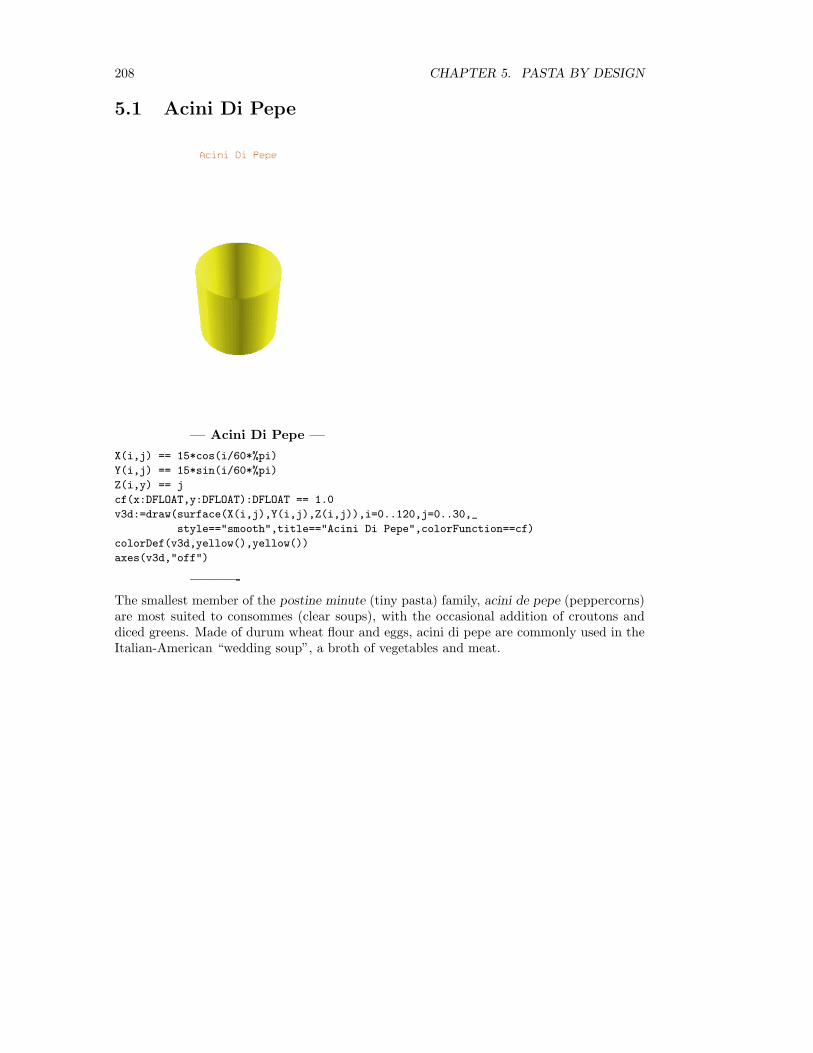
208 CHAPTER 5. PASTA BY DESIGN
5.1 Acini Di Pepe
— Acini Di Pepe —
X(i,j) == 15*cos(i/60*%pi)
Y(i,j) == 15*sin(i/60*%pi)
Z(i,y) == j
cf(x:DFLOAT,y:DFLOAT):DFLOAT == 1.0
v3d:=draw(surface(X(i,j),Y(i,j),Z(i,j)),i=0..120,j=0..30,_
style=="smooth",title=="Acini Di Pepe",colorFunction==cf)
colorDef(v3d,yellow(),yellow())
axes(v3d,"off")
———-
The smallest member of the postine minute (tiny pasta) family, acini de pepe (peppercorns)are most suited to consommes (clear soups), with the occasional addition of croutons anddiced greens. Made of durum wheat flour and eggs, acini di pepe are commonly used in theItalian-American “wedding soup”, a broth of vegetables and meat.

5.2. AGNOLOTTI 209
5.2 Agnolotti
— Agnolotti —
X(i,j) == (10*sin((i/120)*%pi)^(0.5) + _
(1/400)*sin(((3*j)/10)*%pi)) * _
cos(((19*j)/2000)*%pi+0.03*%pi)
Y(i,j) == (10*sin((i/120)*%pi) + _
(1/400)*cos(((30*j)/10)*%pi)) * _
sin(((19*j)/2000)*%pi+0.03*%pi)
Z(i,j) == 5*cos((i/120)*%pi)^5 * sin((j/100)*%pi) - _
5*sin((j/100)*%pi) * cos((i/120)*%pi)^200
cf(x:DFLOAT,y:DFLOAT):DFLOAT == 1.0
v3d:=draw(surface(X(i,j),Y(i,j),Z(i,j)),i=0..60,j=0..100,_
style=="smooth",title=="Agnolotti",colorFunction==cf)
colorDef(v3d,yellow(),yellow())
axes(v3d,"off")
zoom(v3d,0.6,0.6,0.6)
———-
These shell-like ravioli from Piedmont, northern italy, are fashioned from small pieces offlattened dough made of wheat flour and egg, and are often filled with braised veal, port,vegetables or cheese. The true agnolotto should feature a crinkled edge, cut using a flutedpasta wheel. Recommended with melted butter and sage
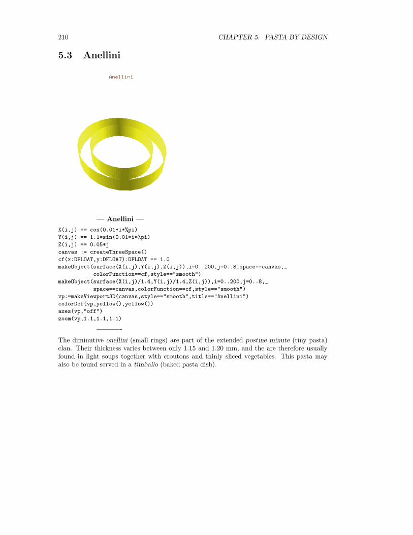
210 CHAPTER 5. PASTA BY DESIGN
5.3 Anellini
— Anellini —
X(i,j) == cos(0.01*i*%pi)
Y(i,j) == 1.1*sin(0.01*i*%pi)
Z(i,j) == 0.05*j
canvas := createThreeSpace()
cf(x:DFLOAT,y:DFLOAT):DFLOAT == 1.0
makeObject(surface(X(i,j),Y(i,j),Z(i,j)),i=0..200,j=0..8,space==canvas,_
colorFunction==cf,style=="smooth")
makeObject(surface(X(i,j)/1.4,Y(i,j)/1.4,Z(i,j)),i=0..200,j=0..8,_
space==canvas,colorFunction==cf,style=="smooth")
vp:=makeViewport3D(canvas,style=="smooth",title=="Anellini")
colorDef(vp,yellow(),yellow())
axes(vp,"off")
zoom(vp,1.1,1.1,1.1)
———-
The diminutive onellini (small rings) are part of the extended postine minute (tiny pasta)clan. Their thickness varies between only 1.15 and 1.20 mm, and the are therefore usuallyfound in light soups together with croutons and thinly sliced vegetables. This pasta mayalso be found served in a timballo (baked pasta dish).

5.4. BUCATINI 211
5.4 Bucatini
— Bucatini —
X(i,j) == 0.3*cos(i/30*%pi)
Y(i,j) == 0.3*sin(i/30*%pi)
Z(i,j) == j/45
canvas := createThreeSpace()
cf(x:DFLOAT,y:DFLOAT):DFLOAT == 1.0
makeObject(surface(X(i,j),Y(i,j),Z(i,j)),i=0..60,j=0..90,space==canvas,_
colorFunction==cf,style=="smooth")
makeObject(surface(X(i,j)/2,Y(i,j)/2,Z(i,j)),i=0..60,j=0..90,space==canvas,_
colorFunction==cf,style=="smooth")
vp:=makeViewport3D(canvas,style=="smooth",title=="Bucatini")
colorDef(vp,yellow(),yellow())
axes(vp,"off")
zoom(vp,2.0,2.0,2.0)
———-
Bucatini (pierced) pasta is commonly served as a pastasciutta (pasta boiled, drained, anddished up with a sauce, rather than in broth). Its best known accompaniment is amatriciana:a hearty traditional sauce made with dried port, Pecorino Romano and tomato sauce, andnamed after the medieval town of Amatrice in central Italy.

212 CHAPTER 5. PASTA BY DESIGN
5.5 Buccoli
— Buccoli —
X(i,j) == (0.7 + 0.2*sin(21*j/250 * %pi))*cos(i/20*%pi)
Y(i,j) == (0.7 + 0.2*sin(21*j/250 * %pi))*sin(i/20*%pi)
Z(i,j) == 39.0*i/1000. + 1.5*sin(j/50*%pi)
cf(x:DFLOAT,y:DFLOAT):DFLOAT == 1.0
v3d:=draw(surface(X(i,j),Y(i,j),Z(i,j)),i=0..200,j=0..25,_
style=="smooth",title=="Buccoli",colorFunction==cf)
colorDef(v3d,yellow(),yellow())
axes(v3d,"off")
zoom(v3d,2.0,2.0,2.0)
———-
A spiral-shaped example from the pasta corta (short pasta) family, and of rather uncertainpedigree, buccoli are suitable in a mushroom and sausage dish. They are also excellent witha tomato aubergine, pesto, and ricotta salad.

5.6. CALAMARETTI 213
5.6 Calamaretti
— Calamaretti —
X(i,j) == cos(i/75*%pi) + 0.1*cos(j/40*%pi) + 0.1*cos(i/75*%pi + j/40*%pi)
Y(i,j) == 1.2*sin(i/75*%pi) + 0.2*sin(j/40*%pi)
Z(i,j) == j/10
cf(x:DFLOAT,y:DFLOAT):DFLOAT == 1.0
v3d:=draw(surface(X(i,j),Y(i,j),Z(i,j)),i=0..150,j=0..20,_
style=="smooth",title=="Calamaretti",colorFunction==cf)
colorDef(v3d,yellow(),yellow())
axes(v3d,"off")
zoom(v3d,1.1,1.1,1.1)
———-
Literally “little squids”, calamaretti are small ring-shaped pasta cooked as pastasciutta(pasta boiled and drained) then dished up with a tomato-, egg-, or cheese-based sauce. Theirshape means that calamaretti hold both chunky and thin sauces equally well. Fittingly, theyare often served with seafood.
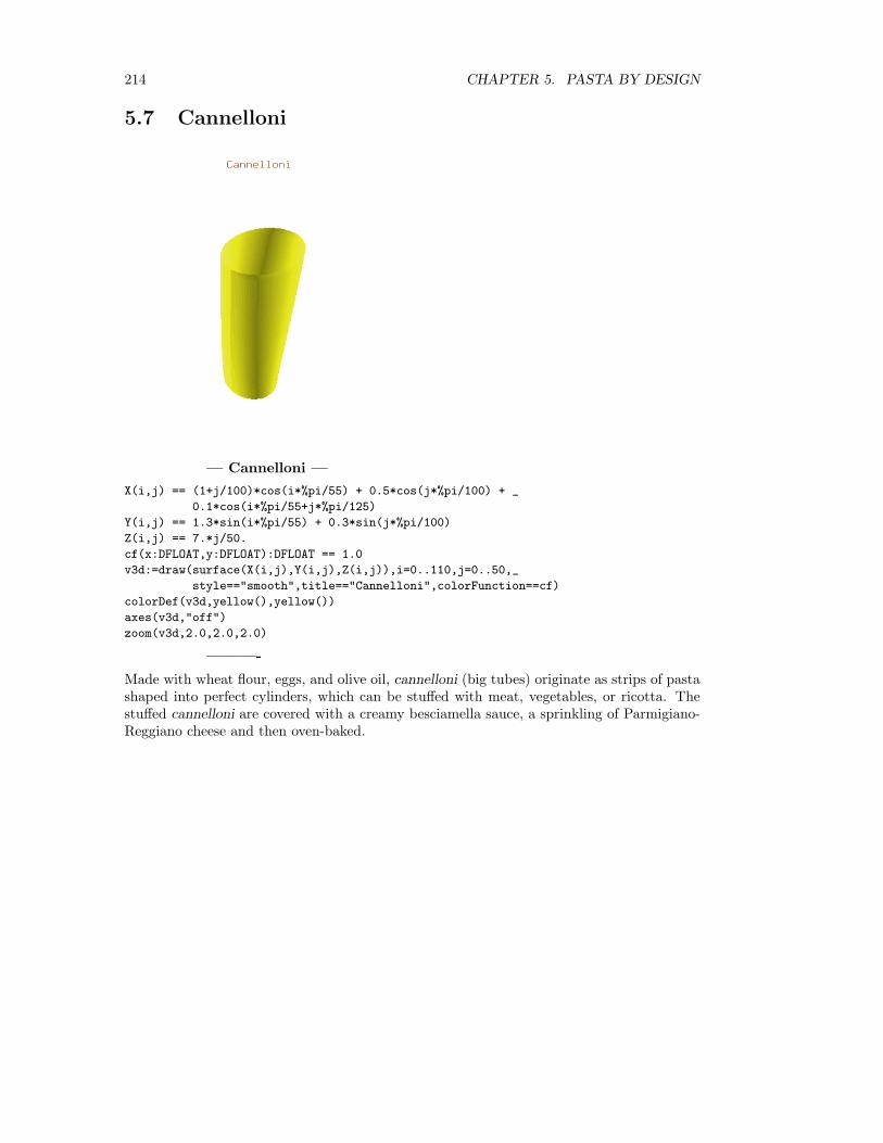
214 CHAPTER 5. PASTA BY DESIGN
5.7 Cannelloni
— Cannelloni —
X(i,j) == (1+j/100)*cos(i*%pi/55) + 0.5*cos(j*%pi/100) + _
0.1*cos(i*%pi/55+j*%pi/125)
Y(i,j) == 1.3*sin(i*%pi/55) + 0.3*sin(j*%pi/100)
Z(i,j) == 7.*j/50.
cf(x:DFLOAT,y:DFLOAT):DFLOAT == 1.0
v3d:=draw(surface(X(i,j),Y(i,j),Z(i,j)),i=0..110,j=0..50,_
style=="smooth",title=="Cannelloni",colorFunction==cf)
colorDef(v3d,yellow(),yellow())
axes(v3d,"off")
zoom(v3d,2.0,2.0,2.0)
———-
Made with wheat flour, eggs, and olive oil, cannelloni (big tubes) originate as strips of pastashaped into perfect cylinders, which can be stuffed with meat, vegetables, or ricotta. Thestuffed cannelloni are covered with a creamy besciamella sauce, a sprinkling of Parmigiano-Reggiano cheese and then oven-baked.

5.8. CANNOLICCHI RIGATI 215
5.8 Cannolicchi Rigati
— Cannolicchi Rigati —
X(i,j) == 8*cos(i*%pi/70) + 0.2*cos(2*i*%pi/7) + 5*cos(j*%pi/100)
Y(i,j) == 8*sin(i*%pi/70) + 0.2*sin(2*i*%pi/7) + 4*sin(j*%pi/100)
Z(i,j) == 6.0*j/5.0
cf(x:DFLOAT,y:DFLOAT):DFLOAT == 1.0
v3d:=draw(surface(X(i,j),Y(i,j),Z(i,j)),i=0..140,j=0..50,_
style=="smooth",title=="Cannolicchi Rigati",colorFunction==cf)
colorDef(v3d,yellow(),yellow())
axes(v3d,"off")
rotate(v3d,2,7)
zoom(v3d,3.0,3.0,3.0)
———-
Known as “little tubes”, cannolicchi exist both in a rigati (grooved) and lisci (smooth) form.These hollow pasta corta (short pasta) come in various diameters and are often served withseafood. Cannolicchi hail from Campania in southern Italy.

216 CHAPTER 5. PASTA BY DESIGN
5.9 Capellini
— Capellini —
X(i,j) == 0.05*cos(2*i*%pi/15) + 0.6*cos(j*%pi/100)
Y(i,j) == 0.05*sin(2*i*%pi/15) + 0.5*sin(j*%pi/100)
Z(i,j) == 7.0*j/100.0
cf(x:DFLOAT,y:DFLOAT):DFLOAT == 1.0
v3d:=draw(surface(X(i,j),Y(i,j),Z(i,j)),i=0..15,j=0..100,_
style=="smooth",title=="Capellini",colorFunction==cf)
colorDef(v3d,yellow(),yellow())
axes(v3d,"off")
zoom(v3d,3.0,3.0,3.0)
———-
An extra-fine rod-like pasta capellini (thin hair) may be served in a light broth, but alsocombine perfectly with butter, nutmeg, or lemon. This variety (or its even more slenderrelative, capelli d’angelo (angel hair) is sometimes used to form the basis of an unusualsweet pasta dish, made with lemons and almonds, called torta ricciolina.

5.10. CAPPELLETTI 217
5.10 Cappelletti
— Cappelletti —
X(i,j) == (0.1 + sin(((3*i)/160)*%pi)) * cos(((2.3*j)/120)*%pi)
Y(i,j) == (0.1 + sin(((3*i)/160)*%pi)) * sin(((2.3*j)/120)*%pi)
Z(i,j) == 0.1 + (1/400.)*j + (0.3 - 0.231*(i/40.)) * cos((i/20.)*%pi)
cf(x:DFLOAT,y:DFLOAT):DFLOAT == 1.0
v3d:=draw(surface(X(i,j),Y(i,j),Z(i,j)),i=0..40,j=0..120,_
style=="smooth",title=="Cappelletti",colorFunction==cf)
colorDef(v3d,yellow(),yellow())
axes(v3d,"off")
zoom(v3d,1.1,1.1,1.1)
———-
This pasta is customarily served as the first course of a traditional north Italian Christmasmeal, dished up in a chicken brodo (broth). Typically, it is the children of a houseold whoprepare the cappelletti (little hats) on Christmas Eve, filling the pasta parcels (made fromwheat flour and fresh eggs) with mixed meats or soft cheeses, such as ricotta.

218 CHAPTER 5. PASTA BY DESIGN
5.11 Casarecce
— Casarecce —
X(i,j) == _
if (i <= 30)_
then 0.5*cos(j*%pi/30)+0.5*cos((2*i+j+16)/40*%pi) _
else cos(j*%pi/40)+0.5*cos(j*%pi/30)+0.5*sin((2*i-j)/40*%pi)
Y(i,j) == _
if (i <= 30)_
then 0.5*sin(j*%pi/30)+0.5*sin((2*i+j+16)/40*%pi) _
else sin(j*%pi/40)+0.5*sin(j*%pi/30)+0.5*cos((2*i-j)/40*%pi)
Z(i,j) == j/4.0
cf(x:DFLOAT,y:DFLOAT):DFLOAT == 1.0
v3d:=draw(surface(X(i,j),Y(i,j),Z(i,j)),i=0..60,j=0..60,_
style=="smooth",title=="Casarecce",colorFunction==cf)
colorDef(v3d,yellow(),yellow())
axes(v3d,"off")
zoom(v3d,3.0,3.0,3.0)
———-
Easily identified by their unique s-shaped cross-section casarecce (home-made) are bestcooked as postasciutta (pasta boiled, drained and dished up with a sauce). Often casarecceare served with a classic ragu and topped with a sprinkle of pepper and Parmigiano-Reggianocheese.

5.12. CASTELLANE 219
5.12 Castellane
— Castellane —
X(i,j) == ((0.3*sin(j*%pi/120)*abs(cos((j+3)*%pi/6)) + _
i^2/720.*(sin(2*j*%pi/300)^2+0.1) + 0.3)) * cos(7*i*%pi/150)
Y(i,j) == ((0.3*sin(j*%pi/120)*abs(cos((j+3)*%pi/6)) + _
i^2/720.*(sin(2*j*%pi/300)^2+0.1) + 0.3)) * sin(7*i*%pi/150)
Z(i,j) == 12*cos(j*%pi/120)
cf(x:DFLOAT,y:DFLOAT):DFLOAT == 1.0
v3d:=draw(surface(X(i,j),Y(i,j),Z(i,j)),i=0..60,j=0..120,_
style=="smooth",title=="Castellane",colorFunction==cf)
colorDef(v3d,yellow(),yellow())
axes(v3d,"off")
viewpoint(v3d,0.0,0.0,45.0)
viewpoint(v3d,5,5,0)
zoom(v3d,1.5,1.5,1.5)
———-
The manufacturer Bailla has recently created this elegant pasta shape. Accordking to itsmaker, they were originally called paguri (hermit crabs) but renamed castellane (castledwellers). The sturdy form and rich nutty taste of castellane stand up to hearty mealsand full-flavoured sauces.

220 CHAPTER 5. PASTA BY DESIGN
5.13 Cavatappi
— Cavatappi —
X(i,j) == (3+2*cos(i*%pi/35)+0.1*cos(2*i*%pi/7))*cos(j*%pi/30)
Y(i,j) == (3+2*cos(i*%pi/35)+0.1*cos(2*i*%pi/7))*sin(j*%pi/30)
Z(i,j) == 3+2*sin(i*%pi/35)+0.1*sin(2*i*%pi/7)+j/6.0
v3d:=draw(surface(X(i,j),Y(i,j),Z(i,j)),i=0..70,j=0..150,_
style=="smooth",title=="Cavatappi")
colorDef(v3d,yellow(),yellow())
axes(v3d,"off")
zoom(v3d,3.0,3.0,3.0)
———-
Perfect with chunky sauces made from lamb or pork, cavatappi (corkscrews) are 36 mm-long,hollow helicoidal tubes. As well as an accompaniment to creamy sauces, such as boscaiola(woodsman’s) sauce, they are also often used in oven-baked cheese-topped dishes, or in saladswith pesto.
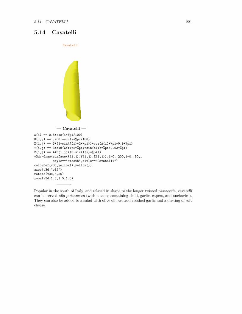
5.14. CAVATELLI 221
5.14 Cavatelli
— Cavatelli —
A(i) == 0.5*cos(i*%pi/100)
B(i,j) == j/60.*sin(i*%pi/100)
X(i,j) == 3*(1-sin(A(i)*2*%pi))*cos(A(i)*%pi+0.9*%pi)
Y(i,j) == 3*sin(A(i)*2*%pi)*sin(A(i)*%pi+0.63*%pi)
Z(i,j) == 4*B(i,j)*(5-sin(A(i)*%pi))
v3d:=draw(surface(X(i,j),Y(i,j),Z(i,j)),i=0..200,j=0..30,_
style=="smooth",title=="Cavatelli")
colorDef(v3d,yellow(),yellow())
axes(v3d,"off")
rotate(v3d,5,50)
zoom(v3d,1.5,1.5,1.5)
———-
Popular in the south of Italy, and related in shape to the longer twisted casareccia, cavatellican be served alla puttanesca (with a sauce containing chilli, garlic, capers, and anchovies).They can also be added to a salad with olive oil, sauteed crushed garlic and a dusting of softcheese.

222 CHAPTER 5. PASTA BY DESIGN
5.15 Chifferi Rigati
— Chifferi Rigati —
X(i,j) == (0.45+0.3*cos(i*%pi/100)+0.005*cos(2*i*%pi/5)) * cos(j*%pi/45) + _
0.15*(j/45.0)^10*cos(i*%pi/100)^3
Y(i,j) == (0.35+j/300.0)*sin(i*%pi/100) + 0.005*sin(2*i*%pi/5)
Z(i,j) == (0.4+0.3*cos(i*%pi/100))*sin(j*%pi/45)
v3d:=draw(surface(X(i,j),Y(i,j),Z(i,j)),i=0..200,j=0..45,_
style=="smooth",title=="Chifferi Rigati")
colorDef(v3d,yellow(),yellow())
axes(v3d,"off")
rotate(v3d,90,180)
———-
This pasta - available in both rigoti (grooved) and lisci (smooth) forms - is typically cooked inbroth or served in rogu alla bolognese, though chifferi rigati also make an excellent additionto salads with carrot, red pepper and courgette. Chifferi rigoti bear a resemblance to, andthe term is a transliteration of, the Austrian ’kipfel’ sweet.

5.16. COLONNE POMPEII 223
5.16 Colonne Pompeii
— Colonne Pompeii —
X0(i,j) == _
if (j <= 50) _
then 2*cos(i*%pi/20) _
else 2*cos(i*%pi/20)*cos(-j*%pi/25)
Y0(i,j) == _
if (j <= 50) _
then 0.0 _
else 2*cos(i*%pi/20)*sin(-j*%pi/25) + 3*sin((j-50)*%pi/200)
Z0(i,j) == _
if (j <= 50) _
then sin(i*%pi/20)+12 _
else sin(i*%pi/20)+6.0*j/25.0
X1(i,j) == _
if (j <= 200) _
then 2*cos(i*%pi/20)*cos(-j*%pi/25+2*%pi/3) _
else 2*cos(i*%pi/20)*sin(-28*%pi/3)
Y1(i,j) == _
if (j <= 200) _
then 2*cos(i*%pi/20)*sin(-j*%pi/20 + 2*%pi/3) + 3*sin(j*%pi/200) _
else 2*cos(i*%pi/20)*sin(-28*%pi/3)
Z1(i,j) == _
if (j <= 200) _
then 12+sin(i*%pi/20)+6.0*j/25.0 _
else sin(i*%pi/20)+60
X2(i,j) == _
if (j <= 200) _
then 2*cos(i*%pi/20)*cos(-j*%pi/25+4*%pi/3) _
else 2*cos(i*%pi/20)*sin(-28*%pi/3)
Y2(i,j) == _
if (j <= 200) _

224 CHAPTER 5. PASTA BY DESIGN
then 2*cos(i*%pi/200)*sin(-j*%pi/25+4*%pi/3)+3*sin(j*%pi/200) _
else 2*cos(i*%pi/20)*sin(-28*%pi/3)
vsp:=createThreeSpace()
makeObject(surface(X0(i,j),Y0(i,j),Z0(i,j)),i=0..10,j=0..250,space==vsp)
makeObject(surface(X1(i,j),Y1(i,j),Z1(i,j)),i=0..10,j=0..250,space==vsp)
makeObject(surface(X2(i,j),Y2(i,j),Z1(i,j)),i=0..10,j=0..250,space==vsp)
vp:=makeViewport3D(vsp,title=="Colonne Pompeii",style=="smooth")
colorDef(vp,yellow(),yellow())
axes(vp,"off")
zoom(vp,3.0,3.0,3.0)
———-
This ornate pasta (originally from Campania, southern Italy) is similar in shape to fusilloni(a large fusilli) but is substantially longer. Colonne Pompeii (columns of Pompeii) are bestserved with a seasoning of fresh basil, pine nuts, finely sliced garlic and olive oil, topped witha sprinkling of freshly grated Parmigiano-Reggiano.

5.17. CONCHIGLIE RIGATE 225
5.17 Conchiglie Rigate
— Conchiglie Rigate —
A(i,j) == 0.25*sin(j*%pi/250)*cos((6*j+25)/25*%pi)
B(i,j) == ((40.0-i)/40.0)*(0.3+sin(j*%pi/250))*%pi
C(i,j) == 2.5*cos(j*%pi/125)+2*sin((40-i)*%pi/80)^10 * _
sin(j*%pi/250)^10*sin(j*%pi/125+1.5*%pi)
X(i,j) == A(i,j)+cos(j*%pi/125)+(5+30*sin(j*%pi/250))*sin(B(i,j)) * _
sin(i/40*(0.1*(1.1+sin(j*%pi/250)^5))*%pi)
Y(i,j) == A(i,j)+(5+30*sin(j*%pi/250))*cos(B(i,j)) * _
sin(i/40*(0.1*(1.1+sin(j*%pi/250)^5))*%pi) + C(i,j)
Z(i,j) == 25.0*cos(j*%pi/250)
v3d:=draw(surface(X(i,j),Y(i,j),Z(i,j)),i=0..40,j=0..250,_
style=="smooth",title=="Conchiglie Rigate")
colorDef(v3d,yellow(),yellow())
axes(v3d,"off")
rotate(v3d,45,45)
zoom(v3d,1.5,1.5,1.5)
———-
Shaped like their namesake, conchiglie (shells) exist in both rigate (grooved) and lisce(smooth) forms. Suited to light tomato sauces, ricotta cheese or pesto genovese, conchigliehold flavourings in their grooves and cunningly designed shell. Smaller versions are used insoups, while larger shells are more commonly served with a sauce.

226 CHAPTER 5. PASTA BY DESIGN
5.18 Conchigliette Lisce
— Conchigliette Lisce —
A(i,j) == (60.0-i)/60.0*(0.5+sin(j*%pi/60))*%pi
B(i,j) == i/60.0*(0.1*(1.1+sin(j*%pi/60)^5))*%pi
C(i,j) == 2.5*cos(j*%pi/30)+2*sin((60-i)*%pi/120)^10 * _
sin(j*%pi/60)^10*sin((j+45)*%pi/30)
X(i,j) == (5+30*sin(j*%pi/60))*sin(A(i,j))*sin(B(i,j))+cos(j*%pi/30)
Y(i,j) == (5+30*sin(j*%pi/60))*cos(A(i,j))*sin(B(i,j))+C(i,j)
Z(i,j) == 25*cos(j*%pi/60)
v3d:=draw(surface(X(i,j),Y(i,j),Z(i,j)),i=0..60,j=0..60,_
style=="smooth",title=="Conchigliette Lisce")
colorDef(v3d,yellow(),yellow())
axes(v3d,"off")
rotate(v3d,45,45)
zoom(v3d,1.5,1.5,1.5)
———-
Typically found in central and southern Italy (notably Campania), conchigliette lisce (smallsmooth shells) can be served in soups such as minestrone. Alternatively, these shells canaccompany a meat- or vegetable-based sauce.

5.19. CONCHIGLIONI RIGATE 227
5.19 Conchiglioni Rigate
— Conchiglioni Rigate —
A(i,j) == 0.25*sin(j*%pi/200)*cos((j+4)*%pi/4)
B(i,j) == i/40.0*(0.1+0.1*sin(j*%pi/200)^6)*%pi
C(i,j) == 2.5*cos(j*%pi/100)+3*sin((40-i)*%pi/80)^10 * _
sin(j*%pi/200)^10*sin((j-150)*%pi/100)
X(i,j) == A(i,j)+(10+30*sin(j*%pi/200)) * _
sin((40.0-i)/40*(0.3+sin(j*%pi/200)^3)*%pi) * _
sin(B(i,j))+cos(j*%pi/100)
Y(i,j) == A(i,j)+(10+30*sin(j*%pi/200)) * _
cos((40.0-i)/40*(0.3+sin(j*%pi/200)^3)*%pi) * _
sin(B(i,j))+C(i,j)
Z(i,j) == 30.0*cos(j*%pi/200)
v3d:=draw(surface(X(i,j),Y(i,j),Z(i,j)),i=0..40,j=0..200,_
style=="smooth",title=="Conchiglioni Rigati")
colorDef(v3d,yellow(),yellow())
axes(v3d,"off")
rotate(v3d,45,45)
zoom(v3d,1.5,1.5,1.5)
———-
The shape of conchiglioni rigate (large ribbed shells) is ideal for holding sauces and fillings(either fish or meat based) and the pasta can be baked in the oven, or placed under a grilland cooked as a gratin. Conchiglioni rigati are often served in the Italian-American dishpasta primavera (pasta in spring sauce) alongside crisp spring vegetables.

228 CHAPTER 5. PASTA BY DESIGN
5.20 Corallini Lisci
— Corallini Lisci —
X(i,j) == 0.8*cos(i*%pi/50)
Y(i,j) == 0.8*sin(i*%pi/50)
Z(i,j) == 3.0*j/50.0
vsp:=createThreeSpace()
makeObject(surface(X(i,j),Y(i,j),Z(i,j)),i=0..140,j=0..70,space==vsp)
makeObject(surface(X(i,j)/2,Y(i,j)/2,Z(i,j)),i=0..140,j=0..70,space==vsp)
vp:=makeViewport3D(vsp,style=="smooth",title=="Corallini Lisci")
colorDef(vp,yellow(),yellow())
axes(vp,"off")
zoom(vp,2.0,2.0,2.0)
———-
Members of the postine minute (tiny pasta) group, corallini lisci (small smooth coral) are socalled because their pierced appearance resembles the coral beads worn as jewelry in Italy.Their small size (no larger than 3.5 mm in diameter) means that corallini are best cookedin broths, such as Tuscan white bean soup.

5.21. CRESTE DI GALLI 229
5.21 Creste Di Galli
— Creste Di Galli —
A(i) == ((1+sin((1.5+i)*%pi))/2)^5
B(i,j) == 0.3*sin(A(i/140.)*%pi+0.5*%pi)^1000*cos(j*%pi/70.0)
C(i,j) == 0.3*cos(A(i/140.)*%pi)^1000*sin(j*%pi/70.0)
X(i,j) == (0.5+0.3*cos(A(i/140.)*2*%pi))*cos(j*%pi/70.0) + _
0.15*(j/70.0)^10*cos(A(i/140.0)*2*%pi)^3 + B(i,j)
Y(i,j) == 0.35*sin(A(i/140.0)*2*%pi) + 0.15*j/70.0*sin(A(i/140.0)*2*%pi)
Z(i,j) == (0.4+0.3*cos(A(i/140.0)*2*%pi))*sin(j*%pi/70.0) + C(i,j)
v3d:=draw(surface(X(i,j),Y(i,j),Z(i,j)),i=0..140,j=0..70,_
style=="smooth",title=="Creste Di Galli")
colorDef(v3d,yellow(),yellow())
axes(v3d,"off")
zoom(v3d,1.5,1.5,1.5)
———-
Part of the pasta ripiena (filled pasta) family, creste di galli (coxcombs) are identical togalletti except for the crest, which is smooth rather than crimped. They may be stuffed,cooked and served in a simple marinara (mariner’s) sauce, which contains tomato, garlic,and basil.

230 CHAPTER 5. PASTA BY DESIGN
5.22 Couretti
— Couretti —
X(i,j) == 2*cos(i*%pi/150)-cos(i*%pi/75)-sin(i*%pi/300)^150 - _
(abs(cos(i*%pi/300)))^5
Y(i,j) == 2*sin(i*%pi/150)-sin(i*%pi/75)
Z(i,j) == j/10.0
v3d:=draw(surface(X(i,j),Y(i,j),Z(i,j)),i=0..300,j=0..10,_
style=="smooth",title=="Couretti")
colorDef(v3d,yellow(),yellow())
axes(v3d,"off")
———-
A romantically shaped scion of the postine minute (tiny pasta) clan, cuoretti (tiny hearts)are minuscule. In fact, along with acini di pepe, they are one of the smallest forms of pasta.Like all postine they may be served in soup, such as cream of chicken.

5.23. DITALI RIGATI 231
5.23 Ditali Rigati
— Ditali Rigati —
X(i,j) == cos(i*%pi/100) + 0.03*cos((7*i)*%pi/40) + 0.25*cos(j*%pi/50)
Y(i,j) == 1.1 * sin(i*%pi/100) + 0.03*sin((7*i)*%pi/40) + 0.25*sin(j*%pi/50)
Z(i,j) == j/10.0
v3d:=draw(surface(X(i,j),Y(i,j),Z(i,j)),i=0..200,j=0..25,_
style=="smooth",title=="Ditali Rigati")
colorDef(v3d,yellow(),yellow())
axes(v3d,"off")
zoom(v3d,1.5,1.5,1.5)
———-
Another speciality of the Campania region of southern Italy, ditali rigati (grooved thimbles)are compact and typically less than 10 mm long. Like other pastine, they are usually foundin soups such as pasta e patate. Their stocky shape makes them a sustaining winter snack,as well as an excellent addition to salads.
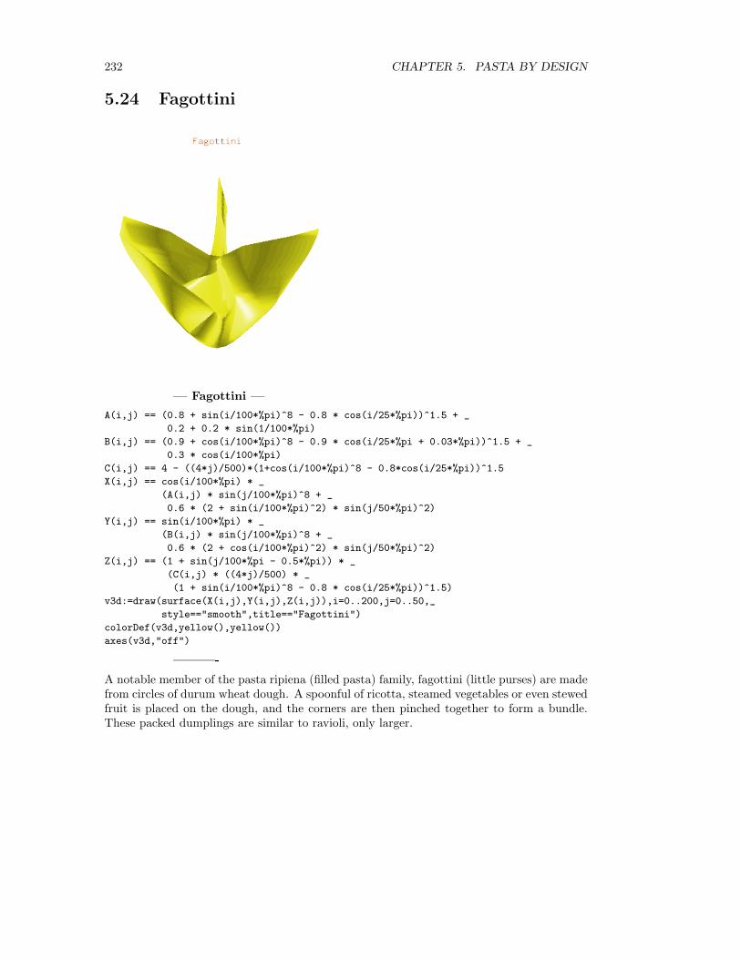
232 CHAPTER 5. PASTA BY DESIGN
5.24 Fagottini
— Fagottini —
A(i,j) == (0.8 + sin(i/100*%pi)^8 - 0.8 * cos(i/25*%pi))^1.5 + _
0.2 + 0.2 * sin(1/100*%pi)
B(i,j) == (0.9 + cos(i/100*%pi)^8 - 0.9 * cos(i/25*%pi + 0.03*%pi))^1.5 + _
0.3 * cos(i/100*%pi)
C(i,j) == 4 - ((4*j)/500)*(1+cos(i/100*%pi)^8 - 0.8*cos(i/25*%pi))^1.5
X(i,j) == cos(i/100*%pi) * _
(A(i,j) * sin(j/100*%pi)^8 + _
0.6 * (2 + sin(i/100*%pi)^2) * sin(j/50*%pi)^2)
Y(i,j) == sin(i/100*%pi) * _
(B(i,j) * sin(j/100*%pi)^8 + _
0.6 * (2 + cos(i/100*%pi)^2) * sin(j/50*%pi)^2)
Z(i,j) == (1 + sin(j/100*%pi - 0.5*%pi)) * _
(C(i,j) * ((4*j)/500) * _
(1 + sin(i/100*%pi)^8 - 0.8 * cos(i/25*%pi))^1.5)
v3d:=draw(surface(X(i,j),Y(i,j),Z(i,j)),i=0..200,j=0..50,_
style=="smooth",title=="Fagottini")
colorDef(v3d,yellow(),yellow())
axes(v3d,"off")
———-
A notable member of the pasta ripiena (filled pasta) family, fagottini (little purses) are madefrom circles of durum wheat dough. A spoonful of ricotta, steamed vegetables or even stewedfruit is placed on the dough, and the corners are then pinched together to form a bundle.These packed dumplings are similar to ravioli, only larger.

5.25. FARFALLE 233
5.25 Farfalle
— Farfalle —
A(i) == sin((7*i+16)*%pi/40)
B(i,j) == (7.0*j/16.0)+4*sin(i*%pi/80)*sin((j-10)*%pi/120)
C(i,j) == 10*cos((i+80)*%pi/80)*sin((j+110)*%pi/100)^9
D(i,j) == (7.0*j/16.0)-4*sin(i*%pi/80)-A(i)*sin((10-j)*%pi/20)
-- E(i,j) was never defined. We guess at a likely function - close but wrong
E(i,j) == _
if ((20 <= i) and (i <= 60)) _
then 7*sin((i+40)*%pi/40)^3*sin((2*j*%pi)/10+1.1*%pi)^9 _
else C(i,j)
F(i) == _
if ((20 <= i) and (i <= 60)) _
then 7*sin((i+40)*%pi/40)^3*sin((j+110)*%pi/100)^9 _
else C(i,j)
X(i,j) == (3.0*i)/8.0+F(i)
Y(i,j) == _
if ((10 <= j) and (j <= 70)) _
then B(i,j)-4*sin(i*%pi/80)*sin((70-j)*%pi/120) _
else if (j <= 10) _
then D(i,j) _
else E(i,j)
Z(i,j) == 3*sin((i+10)*%pi/20)*sin(j*%pi/80)^1.5
v3d:=draw(surface(X(i,j),Y(i,j),Z(i,j)),i=0..80,j=0..80,_
style=="smooth",title=="Farfalle")
colorDef(v3d,yellow(),yellow())
axes(v3d,"off")
zoom(v3d,0.5,0.5,0.5)
———-
A mixture of durum-wheat flour, eggs, and water, farfalle (butterflies) come from the Emilia-Romagnaand Lombardy regions of northern Italy. They are best served in a rich carbonara

234 CHAPTER 5. PASTA BY DESIGN
sauce (made with cream, eggs, and bacon). Depending on se, farfalle might be accompaniedby green peas and chicken or ham.
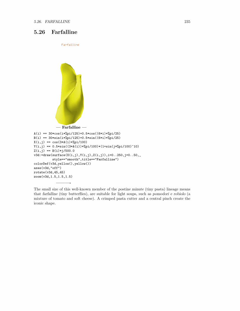
5.26. FARFALLINE 235
5.26 Farfalline
— Farfalline —
A(i) == 30*cos(i*%pi/125)+0.5*cos((6*i)*%pi/25)
B(i) == 30*sin(i*%pi/125)+0.5*sin((6*i)*%pi/25)
X(i,j) == cos(3*A(i)*%pi/100)
Y(i,j) == 0.5*sin((3*A(i))*%pi/100)*(1+sin(j*%pi/100)^10)
Z(i,j) == B(i)*j/500.0
v3d:=draw(surface(X(i,j),Y(i,j),Z(i,j)),i=0..250,j=0..50,_
style=="smooth",title=="Farfalline")
colorDef(v3d,yellow(),yellow())
axes(v3d,"off")
rotate(v3d,45,45)
zoom(v3d,1.5,1.5,1.5)
———-
The small size of this well-known member of the postine minute (tiny pasta) lineage meansthat farfalline (tiny butterflies), are suitable for light soups, such as pomodori e robiolo (amixture of tomato and soft cheese). A crimped pasta cutter and a central pinch create theiconic shape.

236 CHAPTER 5. PASTA BY DESIGN
5.27 Farfalloni
— Farfalloni —
A(i,j) == 10*cos((i+70)*%pi/70)*sin((2*j)*%pi/175+1.1*%pi)^9
B(j) == 0.3*sin((6-j)*%pi/7+0.4*%pi)
C(i,j) == _
if ((17 <= i) and (i <= 52)) _
then 7*sin((i+35)*%pi/35)^3*sin((2*j*%pi)/175+1.1*%pi)^9 _
else A(i,j)
D(i,j) == (j/2.0)+4*sin(i*%pi/70)*sin((j-10)*%pi/100) - _
4*sin(i*%pi/70)*sin((60-j)*%pi/100)
E(i,j) == (j/2.0)+4*sin(i*%pi/70)+0.3*sin((2*i+2.8)*%pi/7)*sin((j-60)*%pi/20)
F(i,j) == (j/2.0)-4*sin(i*%pi/70)-0.3*sin((2*i+2.8)*%pi/7)*sin((10-j)*%pi/20)
X(i,j) == (3.0*i)/7.0+C(i,j)
Y(i,j) == _
if ((10 <= j) and (j <= 60)) _
then D(i,j) _
else if (j <= 10) _
then F(i,j) _
else E(i,j)
Z(i,j) == 3*sin((2*i+17.5)*%pi/35.)*sin(j*%pi/70)^1.5
v3d:=draw(surface(X(i,j),Y(i,j),Z(i,j)),i=0..70,j=0..70,_
style=="smooth",title=="Farfalloni")
colorDef(v3d,yellow(),yellow())
axes(v3d,"off")
zoom(v3d,2.5,2.5,2.5)
———-
Like farfalle, farfalloni (large butterflies) are well matched by a tomato- or butter-based saucewith peas and ham. They are also perfect with marrow vegetables such as roast courgetteor pureed pumpkin, topped with Parmigiano-Reggiano and a sprinkling of noce moscata(nutmeg).

5.28. FESTONATI 237
5.28 Festonati
— Festonati —
X(i,j) == 5*cos(i*%pi/50)+0.5*cos(i*%pi/50)*(1+sin(j*%pi/100)) + _
0.5*cos((i+25)*%pi/25)*(1+sin(j*%pi/5))
Y(i,j) == 5*sin(i*%pi/50)+0.5*sin(i*%pi/50)*(1+sin(j*%pi/100)) + _
0.5*cos(i**%pi/25)*(1+sin(j*%pi/5))
Z(i,j) == j/2.0+2*sin((3*i+25)*%pi/50)
v3d:=draw(surface(X(i,j),Y(i,j),Z(i,j)),i=0..100,j=0..100,_
style=="smooth",title=="Festonati")
colorDef(v3d,yellow(),yellow())
axes(v3d,"off")
zoom(v3d,3.0,3.0,3.0)
———-
This smooth member of the pasta corta (short pasta) family is named after ’festoons’ (dec-orative lengths of fabric with the rippled profile of a garland). Festonati can be served withgrilled aubergine or home-grown tomatoes, topped with grated scamorza, fresh basil, oliveoil, garlic, and red chilli flakes.

238 CHAPTER 5. PASTA BY DESIGN
5.29 Fettuccine
— Fettuccine —
X(i,j) == 1.8*sin((4*i)*%pi/375)
Y(i,y) == 1.6*cos((6*i)*%pi/375)*sin((3*i)*%pi/750)
Z(i,j) == i/75.0 + j/20.0
v3d:=draw(surface(X(i,j),Y(i,j),Z(i,j)),i=0..150,j=0..10,_
style=="smooth",title=="Fettuccine")
colorDef(v3d,yellow(),yellow())
axes(v3d,"off")
———-
This famous pasta lunga (long pasta) is made with durum-wheat flour, water, and in thecase of fettuccine alluovo, eggs ideally within days of laying. Fettuccine (little ribbons) hailfrom the Lazio region. Popular in many dishes, they are an ideal accompaniment to Alfredosauce, a rich mix of cream, parmesan, garlic, and parsley.

5.30. FIOCCHI RIGATI 239
5.30 Fiocchi Rigati
— Fiocchi Rigati —
A(i,j) == 10*cos((i+80)*%pi/80)*sin((j+110)*%pi/100)^9
B(i,j) == 35.0*j/80.0+4*sin(i*%pi/80)*sin((j-10)*%pi/120)
X(i,j) == _
if ((20 <= i) and (i <= 60)) _
then 7*sin((i+40)*%pi/40)^3*sin((j+110)*%pi/100)^9 + 30.0*i/80.0 _
else A(i,j) + 30.0*i/80.0
Y(i,j) == B(i,j)-4*sin(i*%pi/80)*sin((70-j)*%pi/120)
Z(i,j) == 3*sin((1+10)*%pi/20)*sin(j*%pi/80)^1.5-0.7*((sin(3*j*%pi/8)+1)/2)^4
v3d:=draw(surface(X(i,j),Y(i,j),Z(i,j)),i=0..80,j=0..80,_
style=="smooth",title=="Fiocchi Rigati")
colorDef(v3d,yellow(),yellow())
axes(v3d,"off")
zoom(v3d,2.0,2.0,2.0)
———-
A distant relative of the farfalle family, fiocchi rigati (grooved flakes) are smaller than eitherfarfalloni or farfalle, but larger than farfalline. Their corrugated surface collects more saucethan a typical farfalle. For a more unusual disk, fiocchi rigati can be served in a tomato andvodka sauce.

240 CHAPTER 5. PASTA BY DESIGN
5.31 Fisarmoniche
— Fisarmoniche —
X(i,j) == (1.5+3*(i/70.0)^5+4*sin(j*%pi/200)^50)*cos(4*i*%pi/175)
Y(i,j) == (1.5+3*(i/70.0)^5+4*sin(j*%pi/200)^50)*sin(4*i*%pi/175)
Z(i,j) == j/50.0+cos(3*i*%pi/14)*sin(j*%pi/1000)
v3d:=draw(surface(X(i,j),Y(i,j),Z(i,j)),i=0..70,j=0..1000,_
style=="smooth",title=="Fisarmoniche")
colorDef(v3d,yellow(),yellow())
axes(v3d,"off")
zoom(v3d,2.0,2.0,2.0)
———-
Named after the accordion - whose bellows their bunched profiles recall - fisarmoniche areperfect for capturing thick sauces, which cling to their folds. This sturdy pasta is said tohave been invented in the fifteenth century, in the Italian town of Loreto in the Marche, eastcentral Italy.

5.32. FUNGHINI 241
5.32 Funghini
— Funghini —
A(i,j) == 5*cos(i*%pi/150)+0.05*cos(i*%pi/3)*sin(j*%pi/60)^2000
B(i,j) == j/30.0*(5*sin(i*%pi/150)+0.05*sin(i*%pi/3))
C(i,j) == j/10.0*(2*sin(i*%pi/150)+0.05*sin(i*%pi/3))
D(i,j) == _
if (i <= 150) _
then B(i,j) _
else if (j <= 10) _
then C(i,j) _
else 2*sin(i*%pi/150)+0.05*sin(i*%pi/6)
X(i,j) == 0.05*cos(A(i,j)*%pi/5)+0.3*cos(A(i,j)*%pi/5)*sin(3*D(i,j)*%pi/50)^2
Y(i,j) == 0.01*sin(A(i,j)*%pi/5)+0.3*sin(A(i,j)*%pi/5)*sin(3*D(i,j)*%pi/50)^2
Z(i,j) == 0.25*sin((D(i,j)+3)*%pi/10)
v3d:=draw(surface(X(i,j),Y(i,j),Z(i,j)),i=0..300,j=0..30,_
style=="smooth",title=="Funghini")
colorDef(v3d,yellow(),yellow())
axes(v3d,"off")
———-
The modest dimensions of this pastine minute (tiny pasta) make funghini (little mushrooms)especially suitable for soups, such as a minestrone made from chopped and sauteed celeriac.

242 CHAPTER 5. PASTA BY DESIGN
5.33 Fusilli
— Fusilli —
X(i,j) == 6*cos((3*i+10)*%pi/100)*cos(j*%pi/25)
Y(i,j) == 6*sin((3*i+10)*%pi/100)*cos(j*%pi/25)
Z(i,j) == (3.0*i)/20.0+2.5*cos((j+12.5)*%pi/25)
v3d:=draw(surface(X(i,j),Y(i,j),Z(i,j)),i=0..200,j=0..25,_
style=="smooth",title=="Fusilli")
colorDef(v3d,yellow(),yellow())
axes(v3d,"off")
zoom(v3d,2.0,2.0,2.0)
———-
A popular set from the pasta corta (short pasta) family, fusilli (little spindles) were originallymade by quickly wrapping a spaghetto around a large needle. Best served as pastasciutta(pasta boild and drained) with a creamy sauce containing slices of spicy sausage.

5.34. FUSILLI AL FERRETTO 243
5.34 Fusilli al Ferretto
— Fusilli al Ferretto —
A(i,j) == 6.0*i/7.0+15*cos(j*%pi/20)
X(i,j) == (3+1.5*sin(i*%pi/140)^0.5*sin(j*%pi/20))*sin(13*i*%pi/280) + _
5*sin(2*A(i,j)*%pi/135)
Y(i,j) == (3+1.5*sin(i*%pi/140)^0.5*sin(j*%pi/20))*cos(13*i*%pi/280)
Z(i,j) == A(i,j)
v3d:=draw(surface(X(i,j),Y(i,j),Z(i,j)),i=0..140,j=0..40,_
style=="smooth",title=="Fusilli al Ferretto")
colorDef(v3d,yellow(),yellow())
axes(v3d,"off")
zoom(v3d,3.0,3.0,3.0)
———-
To create this Neapolitan variety of fusilli, a small amount of durum-wheat flour is kneadedand placed along a ferretto (small iron stick) that is then rolled between the hands to createa thick irregular twist of dough. The shape is removed and left to dry on a wicker trayknown as a spasa. Fusilli al ferretto are best dished up with a lamb ragu.

244 CHAPTER 5. PASTA BY DESIGN
5.35 Fusilli Capri
— Fusilli Capri —
X(i,j) == 6*cos(j*%pi/50)*cos((i+2.5)*%pi/25)
Y(i,j) == 6*cos(j*%pi/50)*sin((i+2.5)*%pi/25)
Z(i,j) == 2.0*i/3.0 + 14*cos((j+25)*%pi/50)
v3d:=draw(surface(X(i,j),Y(i,j),Z(i,j)),i=0..150,j=0..50,_
style=="smooth",title=="Fusilli Capri")
colorDef(v3d,yellow(),yellow())
axes(v3d,"off")
zoom(v3d,2.5,2.5,2.5)
———-
A longer and more compact regional adaptation of fusilli, fusilli Capri are suited to a heartyragu of lamb or por sausages, or may also be combined with rocket and lemon to form alighter dish.

5.36. FUSILLI LUNGHI BUCATI 245
5.36 Fusilli Lunghi Bucati
— Fusilli Lunghi Bucati —
A(i,j) == 10+cos(i*%pi/10)+2*cos((j+10)*%pi/10)+10*cos((j+140)*%pi/160)
B(i,j) == 20+cos(i*%pi/10)+2*cos((j+10)*%pi/10)
C(i,j) == (j+10.0)*%pi/10.0
D(i,j) == i*%pi/10.0
E(i,j) == 7+20*sin((j-20)*%pi/160)
F(i,j) == 70*(0.1-(j-180.0)/200.0)
X(i,j) == _
if ((20 <= j) and (j <= 180)) _
then A(i,j) _
else if (j <= 20) _
then cos(D(i,j))+2*cos(C(i,j)) _
else B(i,j)
Y(i,j) == _
if ((20 <= j) and (j <= 180)) _
then sin(D(i,j))+2*sin(C(i,j)) _
else sin(D(i,j))+2*sin(C(i,j))
Z(i,j) == _
if ((20 <= j) and (j <= 180)) _
then E(i,j) _
else if (j <= 20) _
then ((7.0*j)/20.0) _
else F(i,j)
v3d:=draw(surface(X(i,j),Y(i,j),Z(i,j)),i=0..20,j=0..200,_
style=="smooth",title=="Fusilli Lunghi Bucati")
colorDef(v3d,yellow(),yellow())
axes(v3d,"off")
zoom(v3d,2.5,2.5,2.5)
———-
246 CHAPTER 5. PASTA BY DESIGN
A distinctive member of the extended fusilli clan, fusilli lunghi bucati (long pierced fusilli)originated in Campania, southern Italy, and have a spring-like profile. Like all fusilli theyare traditionally consumed with a meat-based ragu, but may also be combined with thickvegetable sauces and baked in an oven.

5.37. GALLETTI 247
5.37 Galletti
— Galletti —
A(i) == ((1+sin(i*%pi+1.5*%pi))/2)^5
B(i,j) == 0.4*sin(A(i/140)*%pi+0.5*%pi)^1000*cos(j*%pi/70)
C(i,j) == 0.15*sin(A(i/140)*%pi+0.5*%pi)^1000*cos(j*%pi/7)
D(i,j) == 0.4*cos(A(i/140)*%pi)^1000*sin(j*%pi/70)
X(i,j) == (0.5+0.3*cos(A(i/140)*2*%pi))*cos(j*%pi/70) + _
0.15*(j/70.0)^10*cos(A(i/140)*2*%pi)^3 + B(i,j)
Y(i,j) == 0.35*sin(A(i/140)*2*%pi)+0.15*(j/70.0)*sin(A(i/140)*2*%pi)+C(i,j)
Z(i,j) == (0.4+0.3*cos(A(i/140)*2*%pi))*sin(j*%pi/70) + D(i,j)
v3d:=draw(surface(X(i,j),Y(i,j),Z(i,j)),i=0..140,j=0..70,_
style=="smooth",title=="Galletti")
colorDef(v3d,yellow(),yellow())
axes(v3d,"off")
zoom(v3d,1.5,1.5,1.5)
———-
According to their maker, Barilla, the origin of galletti (small cocks) is uncertain, but theirshape recalls that of the chifferi with the addtion of an undulating crest. Galletti are usuallyserved in tomato sauces, but combine wqually well with a boscaiola (woodsman’s) sauce ofmushrooms.

248 CHAPTER 5. PASTA BY DESIGN
5.38 Garganelli
— Garganelli —
A(i,j) == (i-25.0)/125.0*j
B(i,j) == (i-25.0)/125.0*(150.0-j)
C(i,j) == _
if ((j <= 75) or (i <= 25)) _
then A(i,j) _
else if ((J >= 75) or (i <= 25)) _
then B(i,j) _
else if ((j >= 75) or (i >= 25)) _
then B(i,j) _
else A(i,j)
X(i,j) == 0.1*cos(j*%pi/3)+(3+sin(C(i,j)*%pi/60))*cos(7*C(i,j)*%pi/60)
Y(i,j) == 0.1*sin(j*%pi/3)+(3+sin(C(i,j)*%pi/60))*sin(7*C(i,j)*%pi/60)
Z(i,j) == 6.0*j/25.0+C(i,j)/4.0
v3d:=draw(surface(X(i,j),Y(i,j),Z(i,j)),i=0..50,j=0..150,_
style=="smooth",title=="Garganelli")
colorDef(v3d,yellow(),yellow())
axes(v3d,"off")
zoom(v3d,2.0,2.0,2.0)
viewpoint(v3d,-5,0,0)
———-
A grooved pasta corta (short pasta), similar to maccheroni but with pointed slanting ends,garganelli are shaped like the gullet of a chicken (’garganel’ in the northern Italian Emiliano-Romagnolo dialect). Traditionally cooked in broth, garganelli are also sometimes served inhare sauce with chopped bacon.

5.39. GEMELLI 249
5.39 Gemelli
— Gemelli —
X(i,j) == 6*cos(j*1.9*%pi/50+0.55*%pi)*cos(3.0*i/25.0)
Y(i,j) == 6*cos(j*1.9*%pi/50+0.55*%pi)*sin(3.0*i/25.0)
Z(i,j) == 8*sin(j*1.9*%pi/50+0.55*%pi)+3.0*i/4.0
v3d:=draw(surface(X(i,j),Y(i,j),Z(i,j)),i=0..100,j=0..50,_
style=="smooth",title=="Gemelli")
colorDef(v3d,yellow(),yellow())
axes(v3d,"off")
zoom(v3d,2.5,2.5,2.5)
———-
To create a gemello, a single pasta strand is twisted into a spiral with a deceptively dualappearance. In the south of Italy gemelli (twins) are served with tomato, mozzarella, andbasil, while in the northwest they are preferred with pesto and green beans, or in salads.

250 CHAPTER 5. PASTA BY DESIGN
5.40 Gigli
— Gigli —
X(i,j) == (0.8-0.6*sin(j*%pi/80)^0.5)*cos(i*%pi/50)+0.08*sin(j*%pi/40)
Y(i,j) == (0.8-0.6*sin(j*%pi/80)^0.5)*sin(i*%pi/50)+0.08*sin(j*%pi/40)
Z(i,j) == 1.1*j/40.0+0.7*(1-sin((150-i)*%pi/300))^2
v3d:=draw(surface(X(i,j),Y(i,j),Z(i,j)),i=0..150,j=0..40,_
style=="smooth",title=="Gigli")
colorDef(v3d,yellow(),yellow())
axes(v3d,"off")
zoom(v3d,2.0,2.0,2.0)
———-
With their fluted edges and cone-like shape, gigli resemble small bells (campanelle) or lilies(gigli), after which they are named. Another more recent design, gigli are shaped to capturethick meaty sauces.

5.41. GIGLIO ONDULATO 251
5.41 Giglio Ondulato
— Giglio Ondulato —
A(i,j) == 0.6+0.03*((40.0-j)/40.0)^10*cos((4*i+75)*%pi/15) - _
0.5*sin(j*%pi/80)^0.6
B(i,j) == sin(2*i*%pi/75)+(i/150.0)^10*(0.08*sin(j*%pi/40)+0.03*sin(j*%pi/5))
X(i,j) == A(i,j)*cos(2*i*%pi/75)+(i/150.0)^10 * _
(0.08*sin(j*%pi/40)+0.03*cos(j*%pi/5))
Y(i,j) == (0.6+0.03*((40.0-j)/40.0)^10*sin(4*i*%pi/15)-0.5*sin(j*%pi/80)^0.6)*_
B(i,j)
Z(i,j) == 1.1*j/40.0+0.7*(1-sin((150.0-i)*%pi/300.0))
v3d:=draw(surface(X(i,j),Y(i,j),Z(i,j)),i=0..150,j=0..40,_
style=="smooth",title=="Giglio Ondulato")
colorDef(v3d,yellow(),yellow())
axes(v3d,"off")
zoom(v3d,2.0,2.0,2.0)
———-
Identical to gigli but with crenellated edges, giglio ondulato are made of durum-wheat flourand water.

252 CHAPTER 5. PASTA BY DESIGN
5.42 Gnocchetti Sardi
— Gnocchetti Sardi —
A(j) == 0.8+3*sin(j*%pi/150)^0.8
B(i,j) == cos((2*j+7.5)*%pi/15)
X(i,j) == A(j)*cos(i*%pi/50)+0.2*cos(i*%pi/50)*sin(j*%pi/150)*B(i,j)
Y(i,j) == A(j)*sin(i*%pi/50)+0.2*sin(i*%pi/50)*sin(j*%pi/150)*B(i,j)
Z(i,j) == 13.0*cos(j*%pi/150)
v3d:=draw(surface(X(i,j),Y(i,j),Z(i,j)),i=0..50,j=0..150,_
style=="smooth",title=="Gnocchetti Sardi")
colorDef(v3d,yellow(),yellow())
axes(v3d,"off")
zoom(v3d,1.5,1.5,1.5)
———-
As their name suggests, gnocchetti are simply small gnocchi (or ’dumplings’). They go wellwith ricotta or Pecorino Romano cheese, or served with thick sauces such as a veal ragu.Gnocchetti originated in Sardinia, a Mediterranean island to the west of Italy.

5.43. GNOCCHI 253
5.43 Gnocchi
— Gnocchi —
A(i,j) == i/40.0*sin(j*%pi/130)
B(i,j) == abs(cos((j+13)*%pi/26))
X(i,j) == 0.2*cos(i*1.3*%pi/40)*sin(j*%pi/130)*B(i,j) + _
A(i,j)*cos(i*1.3*%pi/40)
Y(i,j) == 0.2*sin(i*1.3*%pi/40)*sin(j*%pi/130)*B(i,j) + _
A(i,j)*sin(i*1.3*%pi/40)
Z(i,j) == 1.5*cos(j*%pi/130)
v3d:=draw(surface(X(i,j),Y(i,j),Z(i,j)),i=0..40,j=0..130,_
style=="smooth",title=="Gnocchi")
colorDef(v3d,yellow(),yellow())
axes(v3d,"off")
zoom(v3d,1.5,1.5,1.5)
———-
Members of an extended family, gnocchi (dumplings) often resemble a semi-open groovedshell. Their preparation and ingredients (including potato, durum wheat, buckwheat andsemolina) vary according to type. Gnocchi are often added to a sauce made from fontinacheese.

254 CHAPTER 5. PASTA BY DESIGN
5.44 Gramigna
— Gramigna —
X(i,j) == (0.5+5.6*(j/150.0)^2+0.3*cos(2*i*%pi/25))*cos(2.1*j*%pi/150)
Y(i,j) == 0.3*sin(2*i*%pi/25)
Z(i,j) == (0.5+3.2*(j/150.0)^2+0.3*cos(2*i*%pi/25))*sin(2.1*j*%pi/150)
v3d:=draw(surface(X(i,j),Y(i,j),Z(i,j)),i=0..25,j=0..150,_
style=="smooth",title=="Gramigna")
colorDef(v3d,yellow(),yellow())
axes(v3d,"off")
zoom(v3d,2.0,2.0,2.0)
———-
A speciality of the northern Italian region of Emilia-Romagna, gramigna (little weed) aretraditionally served with a chunky sauce of sausages, or accompanied by the world-famousragu alla bolognese. Alternatively, gramigna are sometimes presented alla pomodoro (witha light tomato sauce).
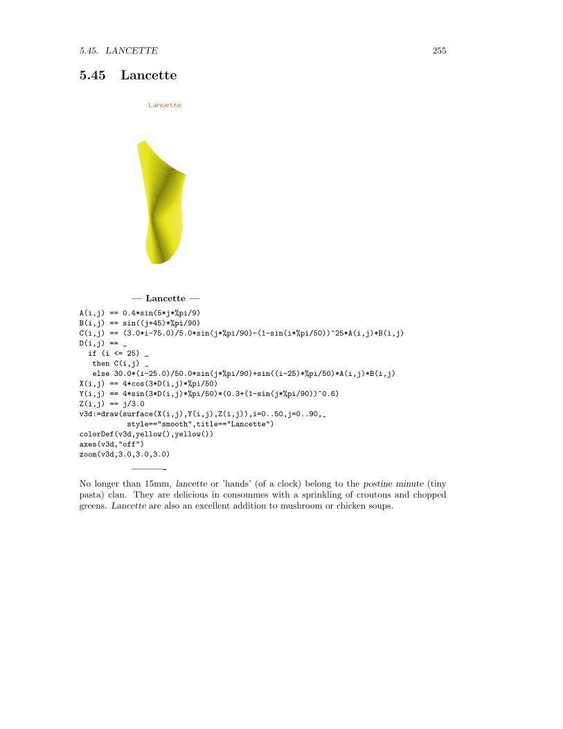
5.45. LANCETTE 255
5.45 Lancette
— Lancette —
A(i,j) == 0.4*sin(5*j*%pi/9)
B(i,j) == sin((j+45)*%pi/90)
C(i,j) == (3.0*i-75.0)/5.0*sin(j*%pi/90)-(1-sin(i*%pi/50))^25*A(i,j)*B(i,j)
D(i,j) == _
if (i <= 25) _
then C(i,j) _
else 30.0*(i-25.0)/50.0*sin(j*%pi/90)+sin((i-25)*%pi/50)*A(i,j)*B(i,j)
X(i,j) == 4*cos(3*D(i,j)*%pi/50)
Y(i,j) == 4*sin(3*D(i,j)*%pi/50)*(0.3+(1-sin(j*%pi/90))^0.6)
Z(i,j) == j/3.0
v3d:=draw(surface(X(i,j),Y(i,j),Z(i,j)),i=0..50,j=0..90,_
style=="smooth",title=="Lancette")
colorDef(v3d,yellow(),yellow())
axes(v3d,"off")
zoom(v3d,3.0,3.0,3.0)
———-
No longer than 15mm, lancette or ’hands’ (of a clock) belong to the postine minute (tinypasta) clan. They are delicious in consommes with a sprinkling of croutons and choppedgreens. Lancette are also an excellent addition to mushroom or chicken soups.

256 CHAPTER 5. PASTA BY DESIGN
5.46 Lasagna Larga Doppia Riccia
— Lasagna Larga Doppia Riccia —
X(i,j) == _
if ((8 <= i) and (i <= 42)) _
then 5.0/6.0+(5.0*i-40.0)/34.0 _
else if (i <= 8) _
then 5.0*i/48.0 _
else 5.0/6.0*(7+(i-42.0)/8)
Y(i,j) == j/15.0
Z(i,j) == _
if ((8 <= i) and (i <= 42)) _
then 0.0 _
else if (i <= 8) _
then (8.0-i)/32.0*cos((j+3)*%pi/6) _
else 0.25*(i-42)/8.0*cos((j+9)*%pi/6)
v3d:=draw(surface(X(i,j),Y(i,j),Z(i,j)),i=0..50,j=0..150,_
style=="smooth",title=="Lasagna Larga Doppia Riccia")
colorDef(v3d,yellow(),yellow())
axes(v3d,"off")
zoom(v3d,3.0,3.0,3.0)
———-
As their name suggests, lasagna larga doppia riccia (large doubly curled lasagna) have twolong undulating edges. The curls give the pasta a variable consistency when cooked, andhelp them to collect sauce. Lasagne are excellent with ricotta and a ragu napoletano, orcooked al forno (at the oven) with a creamy besciamella sauce.

5.47. LINGUINE 257
5.47 Linguine
— Linguine —
X(i,j) == cos(i*%pi/75)
Y(i,j) == 2*sin(i*%pi/75)
Z(i,j) == j/5.0
v3d:=draw(surface(X(i,j),Y(i,j),Z(i,j)),i=0..150,j=0..50,_
style=="smooth",title=="Linguine")
colorDef(v3d,yellow(),yellow())
axes(v3d,"off")
zoom(v3d,2.5,2.5,2.5)
———-
The thinnest member of the bavette (little dribble) family, linguine (little tongues) are bestaccompanied by fresh tomato, herbs, a drop of olive oil, garlic, anchovies, and hot peppers.Linguine may also be served with shellfish sauces, or white sauces of cream and soft cheese,flavoured with lemon, saffron, or ginger.

258 CHAPTER 5. PASTA BY DESIGN
5.48 Lumaconi Rigati
— Lumaconi Rigati —
A(i,j) == 0.45+0.01*cos(i*%pi/3)+j/300.0*abs(cos(i*%pi/240))*cos(i*%pi/120)^20
B(i,j) == j/300.0*abs(cos(i*%pi/240))*sin(i*%pi/120) + _
0.125*(j/60.0)^6*sin(i*%pi/120)
X(i,j) == (0.4*cos(i*%pi/120)+A(i,j))*cos(j*%pi/60) + _
0.48*(j/60.0)^6*sin((i+60)*%pi/120)^3
Y(i,j) == 0.5*sin(i*%pi/120)+0.01*sin(i*%pi/3)+B(i,j)
Z(i,j) == (0.45+0.4*cos(i*%pi/120))*sin(j*%pi/60)
v3d:=draw(surface(X(i,j),Y(i,j),Z(i,j)),i=0..240,j=0..60,_
style=="smooth",title=="Lumaconi Rigati")
colorDef(v3d,yellow(),yellow())
axes(v3d,"off")
rotate(v3d,90,180)
———-
Originally from Campania and Liguria, lumaconi rigati (big ribbed snails) can be stuffedwith a wide range of fillings, including spinach and ricotta cheese. Like cannelloni, theycan then be covered in besciamella and cooked in the oven. Smaller members of the family(lumache) are also available.

5.49. MACCHERONI 259
5.49 Maccheroni
— Maccheroni —
X(i,j) == 8*cos(i*%pi/75)+0.2*cos(4*i*%pi/15)+5*cos(j*%pi/100)
Y(i,j) == 8*sin(i*%pi/75)+0.2*sin(4*i*%pi/15)+4*sin(j*%pi/100)
Z(i,j) == 6.0*j/5.0
v3d:=draw(surface(X(i,j),Y(i,j),Z(i,j)),i=0..150,j=0..50,_
style=="smooth",title=="Maccheroni")
colorDef(v3d,yellow(),yellow())
axes(v3d,"off")
zoom(v3d,2.0,2.0,2.0)
———-
The origin of the name maccheroni is uncertain. It is used generically to describe a hollowpasta corta (short pasta) that is moade of durum-wheat flour and perhasp eggs. The pastacan be served con le sarde (with sardines) - a dish enhanced by a touch of fennel.

260 CHAPTER 5. PASTA BY DESIGN
5.50 Maccheroni Alla Chitarra
— Maccheroni Alla Chitarra —
X(i,j) == 0.05*cos(i*%pi/60)^3 + 0.05*cos(i*%pi/60)
Y(i,j) == 0.05*sin(i*%pi/60)^3 + 0.05*sin(i*%pi/60)
Z(i,j) == j/60.0
v3d:=draw(surface(X(i,j),Y(i,j),Z(i,j)),i=0..120,j=0..60,_
style=="smooth",title=="Maccheroni Alla Chitarra")
colorDef(v3d,yellow(),yellow())
axes(v3d,"off")
zoom(v3d,2.5,2.5,2.5)
———-
Coming from the central Italian region of Abruzzo, maccheroni alla chitarra (guitar mac-cheroni) have a square cross-section, produced when a thin sheet of pasta is pressed througha frame of closely ranged wires (or chitarra) that lends the pasta its name. Usually sevedwith a mutton ragu, or pallottelle (veal meatballs).

5.51. MAFALDINE 261
5.51 Mafaldine
— Mafaldine —
X(i,j) == 7.0*i/18.0
Y(i,j) == j/3.0
Z(i,j) == _
if ((6 <= i) and (i <= 24)) _
then 0.0 _
else if (i <= 6) _
then (6.0-i)/6.0*cos((j+5)*%pi/10) _
else (i-24.0)/6.0*cos((j+15)*%pi/10)
v3d:=draw(surface(X(i,j),Y(i,j),Z(i,j)),i=0..30,j=0..150,_
style=="smooth",title=="Mafaldine")
colorDef(v3d,yellow(),yellow())
axes(v3d,"off")
zoom(v3d,2.0,2.0,2.0)
———-
Named at the turn of the twentieth century after Princess Mafalda of the House of Savoy,mafaldine are thin flat sheets of durum-wheat flour pasta with a rippled finish on each longedge. They are generally served with meaty sauces such as ragu napoletano or in seafooddishes.
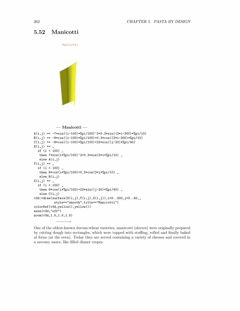
262 CHAPTER 5. PASTA BY DESIGN
5.52 Manicotti
— Manicotti —
A(i,j) == -7*sin((i-100)*%pi/100)^2+0.3*sin((3*i-300)*%pi/10)
B(i,j) == -8*cos((i-100)*%pi/100)+0.3*cos((3*i-300)*%pi/10)
C(i,j) == -8*cos((i-100)*%pi/100)+22*sin((j-20)*%pi/40)
X(i,j) == _
if (i < 100) _
then 7*sin(i*%pi/100)^2+0.3*sin(3*i*%pi/10) _
else A(i,j)
Y(i,j) == _
if (i < 100) _
then 8*cos(i*%pi/100)+0.3*cos(3*i*%pi/10) _
else B(i,j)
Z(i,j) == _
if (i < 100) _
then 8*cos(i*%pi/100)+22*sin((j-20)*%pi/40) _
else C(i,j)
v3d:=draw(surface(X(i,j),Y(i,j),Z(i,j)),i=0..200,j=0..40,_
style=="smooth",title=="Manicotti")
colorDef(v3d,yellow(),yellow())
axes(v3d,"off")
zoom(v3d,1.5,1.5,1.5)
———-
One of the oldest-known durum-wheat varieties, manicotti (sleeves) were originally preparedby cutting dough into rectangles, which were topped with stuffing, rolled and finally bakedal forno (at the oven). Today they are served containing a variety of cheeses and covered ina savoury sauce, like filled dinner crepes.

5.53. ORECCHIETTE 263
5.53 Orecchiette
— Orecchiette —
X(i,j) == 2.0*j/3.0*cos(i*%pi/75)+0.3*cos(2*i*%pi/15)
Y(i,j) == 10*sin(i*%pi/75)
Z(i,j) == 0.1*cos(i*%pi/3)+5*(0.5+0.5*cos(2*i*%pi/75))^4*cos(j*%pi/30)^2 + _
1.5*(0.5+0.5*cos(2*i*%pi/75))^5*sin(j*%pi/30)^10
v3d:=draw(surface(X(i,j),Y(i,j),Z(i,j)),i=0..150,j=0..15,_
style=="smooth",title=="Orecchiette")
colorDef(v3d,yellow(),yellow())
axes(v3d,"off")
———-
This pasta is popular in the southeastern coastal region of Puglia in Italy, where it is cus-tomarily cooked in dishes with rapini, a relative of broccoli that grows plentifully in the area.Orecchiette (litte ears) also pair well with other vegetables such as beans, and with saltyseasonings such as anchovies, capers, or olives.

264 CHAPTER 5. PASTA BY DESIGN
5.54 Paccheri
— Paccheri —
X(i,j) == (j+60.0)/60.0*cos(i*%pi/75)+0.5*cos(j*%pi/60)+cos((i+j)*%pi/75)
Y(i,j) == 2.6*sin(i*%pi/75)+0.3*sin(j*%pi/60)
Z(i,j) == 7.0*j/30.0
v3d:=draw(surface(X(i,j),Y(i,j),Z(i,j)),i=0..150,j=0..30,_
style=="smooth",title=="Paccheri")
colorDef(v3d,yellow(),yellow())
axes(v3d,"off")
zoom(v3d,2.0,2.0,2.0)
———-
Part of the pasta corta (short pasta) family, paccheri are ribbed pasta cylinders that (due totheir large size) are recommended with aubergine, seafood, or indeed any chunky sauce. Itis thought the name stems from the term paccare, which means ’to smack’ in the southernItalian region of Campania.

5.55. PAPPARDELLE 265
5.55 Pappardelle
— Pappardelle —
A(i,j) == cos(i*%pi/80)+(3.0*j)/50.0*sin(21*i*%pi/800)
B(i,j) == sin(i*%pi/3200)^0.1*sin(i*%pi/80)
C(i,j) == 3.0*j/50.0+0.5*sin(i*%pi/200)
D(i,j) == cos(i*%pi/80)+3.0*j/50.0*sin(21*i*%pi/800)
E(i,j) == sin(i*%pi/3200)^0.5*sin(i*%pi/80)
F(i,j) == 3.0*j/50.0+0.5*sin(i*%pi/200)
vsp:=createThreeSpace()
makeObject(surface(A(i,j),B(i,j),C(i,j)),i=0..800,j=0..5,space==vsp)
makeObject(surface(0.6*D(i,j),0.8*E(i,j),0.9*F(i,j)),i=0..800,j=0..5,_
space==vsp)
vp:=makeViewport3D(vsp,style=="smooth",title=="Pappardelle")
colorDef(vp,yellow(),yellow())
axes(vp,"off")
———-
This pasta lunga (long pasta) is often cooked with duck, pigeon, or other game fowl. Pap-pardelle are so popular that towns in Italy hold festivals in their honour, such as the Sagradelle Pappardelle al Cinghiale (Feast of the Pappardelle and Boar) in Torre Alfina, centralItaly.

266 CHAPTER 5. PASTA BY DESIGN
5.56 Penne Rigate
— Penne Rigate —
X(i,j) == _
if (i < 85) _
then 4*sin(i*%pi/85)^2+0.1*sin(6*i*%pi/17) _
else -4*sin((i-85)*%pi/85)^2+0.1*sin(6*(i-85)*%pi/17)
Y(i,j) == _
if (i < 85) _
then 4*cos(i*%pi/85)+0.1*cos(6*i*%pi/17) _
else -4*cos((i-85)*%pi/85)+0.1*cos(6*(i-85)*%pi/17)
Z(i,j) == _
if (i < 85) _
then 7*cos(i*%pi/85)+15*sin((j-20)*%pi/40) _
else -7*cos((i-85)*%pi/85)+15*sin((j-20)*%pi/40)
v3d:=draw(surface(X(i,j),Y(i,j),Z(i,j)),i=0..170,j=0..40,_
style=="smooth",title=="Penne Rigate")
colorDef(v3d,yellow(),yellow())
axes(v3d,"off")
zoom(v3d,2.0,2.0,2.0)
———-
A versatile pasta, penne rigate (grooved quills) come from Campania, in southern Italy, andbelong to the pasta corta (short pasta) family. they can be served with spicy arrabbiata(angry) sauce, which gets its name from the chillies and red peppers it contains.

5.57. PENNONI LISCI 267
5.57 Pennoni Lisci
— Pennoni Lisci —
X(i,j) == _
if (i < 100) _
then 7*sin(i*%pi/100)^2 _
else -7*sin((i-100)*%pi/100)^2
Y(i,j) == _
if (i < 100) _
then 8*cos(i*%pi/100) _
else -8*cos((i-100)*%pi/100)
Z(i,j) == _
if (i < 100) _
then 12*cos(i*%pi/100)+15*sin((j-20)*%pi/40) _
else -12*cos((i-100)*%pi/100)+15*sin((j-20)*%pi/40)
v3d:=draw(surface(X(i,j),Y(i,j),Z(i,j)),i=0..200,j=0..40,_
style=="smooth",title=="Pennoni Lisci")
colorDef(v3d,yellow(),yellow())
axes(v3d,"off")
zoom(v3d,2.0,2.0,2.0)
———-
Similar in appearance to penne rigate, but larger and without the grooves, pennoni (largequills) require a more oily sauce (perhaps containing sliced chorizo) to cling to their smoothsurface.

268 CHAPTER 5. PASTA BY DESIGN
5.58 Pennoni Rigati
— Pennoni Rigati —
A(i,j) == -7*sin((i-100)*%pi/100)^2+0.2*sin((3*i-300)*%pi/10)
B(i,j) == -8*cos((i-100)*%pi/100)+0.2*cos((3*i-300)*%pi/10)
C(i,j) == -12*cos((i-100)*%pi/100)+15*sin((j-20)*%pi/40)
X(i,j) == _
if (i < 100) _
then 7*sin(i*%pi/100)^2+0.15*sin(3*i*%pi/10) _
else A(i,j)
Y(i,j) == _
if (i < 100) _
then 8*cos(i*%pi/100)+0.15*cos(3*i*%pi/10) _
else B(i,j)
Z(i,j) == _
if (i < 100) _
then 12*cos(i*%pi/100)+15*sin((j-20)*%pi/40) _
else C(i,j)
v3d:=draw(surface(X(i,j),Y(i,j),Z(i,j)),i=0..200,j=0..40,_
style=="smooth",title=="Pennoni Rigati")
colorDef(v3d,yellow(),yellow())
axes(v3d,"off")
zoom(v3d,2.0,2.0,2.0)
———-
The angled trim of the penne pasta family makes its members easy to recognize. Pennonirigati (large grooved quills) are the ridged version of pennoni, and can be stuffed and cooked.

5.59. PUNTALETTE 269
5.59 Puntalette
— Puntalette —
X(i,j) == 1.4*sin(j*%pi/80)^1.2*cos(i*%pi/40)
Y(i,j) == 2.5*sin(j*%pi/80)^1.2*sin(i*%pi/40)
Z(i,j) == 8*cos(j*%pi/80)
v3d:=draw(surface(X(i,j),Y(i,j),Z(i,j)),i=0..80,j=0..80,_
style=="smooth",title=="Puntalette")
colorDef(v3d,yellow(),yellow())
axes(v3d,"off")
zoom(v3d,1.5,1.5,1.5)
———-
Another member of the pastine minute (tiny pasta) family, puntalette (tiny tips) are about9 mm long, and no thicker than 3 mm. Like most pastine, they are best consumed in creamysoups, or perhaps in a salad.

270 CHAPTER 5. PASTA BY DESIGN
5.60 Quadrefiore
— Quadrefiore —
X(i,j) == 2*cos(i*%pi/250)*(abs(sin(3*i*%pi/250)))^20 + _
(0.6+0.9*sin(j*%pi/50))*cos(i*%pi/250)+0.2*cos(4*j*%pi/25)
Y(i,j) == 2*sin(i*%pi/250)*(abs(sin(3*i*%pi/250)))^20 + _
(0.6+0.9*sin(j*%pi/50))*sin(i*%pi/250)+1.5*sin(j*%pi/50)
Z(i,j) == 3.0*j/10.0
v3d:=draw(surface(X(i,j),Y(i,j),Z(i,j)),i=0..500,j=0..50,_
style=="smooth",title=="Quadrefiore")
colorDef(v3d,yellow(),yellow())
axes(v3d,"off")
zoom(v3d,2.5,2.5,2.5)
———-
An uncommon variety of pasta corta (short pasta), quadrefiori (square flowers) are sturdy,with rippled edges running down their lengths. Francis Ford Coppola, the maker and dis-tributor, uses antique bronze moulds and wooden drying racks to achieve an authentic formand consistency.

5.61. QUADRETTI 271
5.61 Quadretti
— Quadretti —
X(i,j) == 3.0*i/14.0
Y(i,j) == 3.0*j/14.0
Z(i,j) == 0.0
v3d:=draw(surface(X(i,j),Y(i,j),Z(i,j)),i=0..70,j=0..70,_
style=="smooth",title=="Quadretti")
colorDef(v3d,yellow(),yellow())
axes(v3d,"off")
zoom(v3d,1.5,1.5,1.5)
———-
These flat shapes are made with durum-wheat flour, eggs, and even nutmeg. Quadretti (tinysquares) are a classic pastine prepared using the leftovers of larger pasta sheets, and can beserved as part of a traditional fish broth, or in soups containing fava beans. Their smallshape means that they need only be cooked for a short time.

272 CHAPTER 5. PASTA BY DESIGN
5.62 Racchette
— Racchette —
A(i) == sin(i*%pi/2000)^0.5
X0(i,j) == 2*cos((i+1500)*%pi/1500)+0.65*cos((i+750)*%pi/1500) + _
2*(abs(cos(i*%pi/300)))^100*cos(i*%pi/1500)
Y0(i,j) == 2.4*sin((i+1500)*%pi/1500)+0.1*sin(i*%pi/1500) + _
2.3*(abs(sin(i*%pi/300)))^100*sin(i*%pi/1500)
X1(i,j) == _
if (i <= 2000) _
then 2.1*cos((2*A(i)+1)*%pi)+0.65*cos((2*A(i)+0.5)*%pi)+_
2.5*sin((A(i)+1.83)*%pi)^500 _
else -2.1
Y1(i,j) == _
if (i <= 2000) _
then 2.5*sin((2*A(i)+1)*%pi)+0.1*sin(A(i)*2*%pi)+_
3*sin((A(i)+1.83)*%pi)^500 _
else 0.0
Z(i,j) == j/4.0
vsp:=createThreeSpace()
makeObject(surface(X0(i,j),Y0(i,j),Z(i,j)),i=0..3000,j=0..4,space==vsp)
makeObject(surface(X1(i,j),Y1(i,j),Z(i,j)),i=0..3000,j=0..4,space==vsp)
vp:=makeViewport3D(vsp,style=="smooth",title=="Racchette")
colorDef(vp,yellow(),yellow())
axes(vp,"off")
———-
Usually served in salads, racchette (rackets) suit crunchy pine nuts, sliced asparagus andfresh peas. Alternatively, the addition of diced watermelon or pomegranate seeds can createa light-tasking snack.
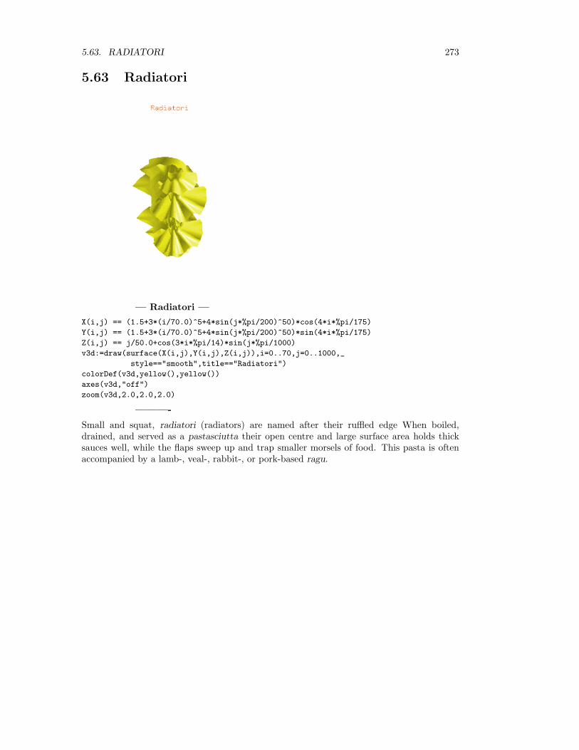
5.63. RADIATORI 273
5.63 Radiatori
— Radiatori —
X(i,j) == (1.5+3*(i/70.0)^5+4*sin(j*%pi/200)^50)*cos(4*i*%pi/175)
Y(i,j) == (1.5+3*(i/70.0)^5+4*sin(j*%pi/200)^50)*sin(4*i*%pi/175)
Z(i,j) == j/50.0+cos(3*i*%pi/14)*sin(j*%pi/1000)
v3d:=draw(surface(X(i,j),Y(i,j),Z(i,j)),i=0..70,j=0..1000,_
style=="smooth",title=="Radiatori")
colorDef(v3d,yellow(),yellow())
axes(v3d,"off")
zoom(v3d,2.0,2.0,2.0)
———-
Small and squat, radiatori (radiators) are named after their ruffled edge When boiled,drained, and served as a pastasciutta their open centre and large surface area holds thicksauces well, while the flaps sweep up and trap smaller morsels of food. This pasta is oftenaccompanied by a lamb-, veal-, rabbit-, or pork-based ragu.

274 CHAPTER 5. PASTA BY DESIGN
5.64 Ravioli Quadrati
— Ravioli Quadrati —
X(i,j) == i/2.0+0.4*sin((j+2.5)*%pi/5) * _
(sin(i*%pi/200)^0.2 - cos(i*%pi/200)^0.2)
Y(i,j) == j/2.0+0.4*sin((11*i+25)*%pi/50) * _
(sin(j*%pi/200)^0.2 - cos(j*%pi/200)^0.2)
Z(i,j) == _
if (((10 < j) and (j < 90)) or ((10 < i) and (i < 90))) _
then 10*sin((i-10)*%pi/80)^0.6*sin((j-10)*%pi/80)^0.6 _
else if ((10 > j) or (10 > i)) _
then 0.0 _
else 0.0
v3d:=draw(surface(X(i,j),Y(i,j),Z(i,j)),i=0..99,j=0..99,_
style=="smooth",title=="Ravioli Quadrati")
colorDef(v3d,yellow(),yellow())
axes(v3d,"off")
zoom(v3d,2.0,2.0,2.0)
———-
Except for the square outline, ravioli quadrati (square ravioli) are made in an identical fashionto ravioli tondi (round ravioli). Other variations on the theme include crescents, triangles,and hearts. Some suggest the name ravioli derives from the verb meaning ’to wrap’, otherslink it with rapa, the Italian word for turnip.

5.65. RAVIOLI TONDI 275
5.65 Ravioli Tondi
— Ravioli Tondi —
X(i,j) == 5.0*i/8.0+0.5*sin((j+2)*%pi/4) * _
(sin(i*%pi/160)^0.2-cos(i*%pi/160)^0.2)
Y(i,j) == 5.0*j/8.0+0.5*sin((i+2)*%pi/4) * _
(sin(j*%pi/160)^0.2-cos(j*%pi/160)^0.2)
Z(i,j) == _
if (600 >= ((i-40)^2+(j-40)^2)) _
then 0.5*sqrt(600 - (i-40)^2-(j-40)^2) _
else 0.0
v3d:=draw(surface(X(i,j),Y(i,j),Z(i,j)),i=0..80,j=0..80,_
style=="smooth",title=="Ravioli Tondi")
colorDef(v3d,yellow(),yellow())
axes(v3d,"off")
zoom(v3d,2.0,2.0,2.0)
———-
By far the best-known pasta ripiena (filled pasta), ravioli tondi (round ravioli) are made bysealing a filling between two layers of dough made from wheat flour and egg. Fillings varyenormously, from lavish pairings of meat and cheese, to more deleicate centres of mushrooms,spinach, or even nettle.

276 CHAPTER 5. PASTA BY DESIGN
5.66 Riccioli
— Riccioli —
X(i,j) == (2+8*sin(i*%pi/100)+9*sin((11*j+100)*%pi/400)^2)*cos(4*i*%pi/125)
Y(i,j) == (2+8*sin(i*%pi/100)+9*sin((11*j+100)*%pi/400)^2)*sin(4*i*%pi/125)
Z(i,j) == j/4.0
v3d:=draw(surface(X(i,j),Y(i,j),Z(i,j)),i=0..50,j=0..200,_
style=="smooth",title=="Riccioli")
colorDef(v3d,yellow(),yellow())
axes(v3d,"off")
zoom(v3d,2.0,2.0,2.0)
———-
A well-know pasta corta (short pasta), riccioli (curls) originated in the Emilia-Romagnaregion of northern Italy. Their ribbed exterior and hollow shape mean riccioli can retain alarge quantity of sauce.

5.67. RICCIOLI AL CINQUE SAPORI 277
5.67 Riccioli al Cinque Sapori
— Riccioli al Cinque Sapori —
X(i,j) == 1.5*cos(i*%pi/20)*(1+0.5*sin(j*%pi/25)*sin(i*%pi/40) + _
0.43*sin((j+18.75)*%pi/25)*cos(i*%pi/40))+2*cos(j*%pi/50)
Y(i,j) == 1.5*sin(i*%pi/20)^3+cos(j*%pi/25)
Z(i,j) == sin(j*%pi/100)+20*cos(j*%pi/200)^2
v3d:=draw(surface(X(i,j),Y(i,j),Z(i,j)),i=0..20,j=0..100,_
style=="smooth",title=="Riccioli al Cinque Sapori")
colorDef(v3d,yellow(),yellow())
axes(v3d,"off")
zoom(v3d,2.5,2.5,2.5)
———-
Riccioli and riccioli al cinque sapori (curls in five flavors) are both members of the pasta corta(small pasta) family, without being related by structural similarities. Made of durum-wheatflour, riccioli al cinque sapori get their color from the addition of spinach, tomato, beetroot,and turmeric, and are usually served in broth.

278 CHAPTER 5. PASTA BY DESIGN
5.68 Rigatoni
— Rigatoni —
X(i,j) == 0.2*sin((7*i+15)*%pi/30)+2*cos((j+60)*%pi/120) + _
(7+(60-j)/60.0*sin(i*%pi/240))*cos(i*%pi/120)
Y(i,j) == 0.2*sin(7*i*%pi/30)+(8+0.1*(60-j)/60+j/30*cos(i*%pi/240)) * _
sin(i*%pi/120)
Z(i,j) == j/2.0
v3d:=draw(surface(X(i,j),Y(i,j),Z(i,j)),i=0..240,j=0..60,_
style=="smooth",title=="Rigatoni")
colorDef(v3d,yellow(),yellow())
axes(v3d,"off")
zoom(v3d,2.0,2.0,2.0)
———-
Members of the pasta corta (short pasta) branch, and originally from southern Italy, rigatoni(large ridges) are very versitile. Their robust shape holds cream or tomato sauces well, butrigatoni are best eaten with sausages or game meat, mushrooms, and black pepper.

5.69. ROMBI 279
5.69 Rombi
— Rombi —
X(i,j) == _
if ((13 <= i) and (i <= 37)) _
then i/20.0+j/25.0-1/20.0 _
else if (i <= 13) _
then 3.0*i/65.0+j/25.0 _
else 6/65.0+3.0*i/65.0+j/25.0
Y(i,j) == j/25.0
Z(i,j) == _
if ((13 <= i) and (i <= 37)) _
then 0.0 _
else if (i <= 13) _
then 0.2*((13.0-i)/13.0)*cos((2.0*j+12.5)*%pi/25) _
else (i-37.0)/65.0*cos((2.0*j+37.5)*%pi/25)
v3d:=draw(surface(X(i,j),Y(i,j),Z(i,j)),i=0..50,j=0..50,_
style=="smooth",title=="Rombi")
colorDef(v3d,yellow(),yellow())
axes(v3d,"off")
zoom(v3d,3.0,3.0,3.0)
———-
A lesser-known pasta corta, rombi (rhombuses) feature two curled edges like lasagna doppiariccia, however, they are smaller and sheared on the diagonal. Generally served with sauceand pastasciutta or in brodo (in broth), according to size.

280 CHAPTER 5. PASTA BY DESIGN
5.70 Rotelle
— Rotelle —
X0(i,j) == 0.5*cos(i*%pi/1000)+1.5*(abs(sin(3*i*%pi/1000)))^50*cos(i*%pi/1000)
Y0(i,j) == 0.5*sin(i*%pi/1000)+1.5*(abs(sin(3*i*%pi/1000)))^50*sin(i*%pi/1000)
X1(i,j) == _
if (i <= 666) _
then 2*cos(3*i*%pi/1000)+0.03*cos(93*i*%pi/1000) _
else 2.03
Y1(i,j) == _
if (i <= 666) _
then 2.05*sin(3*i*%pi/1000)+0.03*sin(93*i*%pi/1000) _
else 0.0
Z(i,j) == j/5.0
vsp:=createThreeSpace()
makeObject(surface(X0(i,j),Y0(i,j),Z(i,j)),i=0..2000,j=0..5,space==vsp)
makeObject(surface(X1(i,j),Y1(i,j),Z(i,j)),i=0..2000,j=0..5,space==vsp)
vp:=makeViewport3D(vsp,style=="smooth",title=="Rotelle")
colorDef(vp,yellow(),yellow())
axes(vp,"off")
———-
A modern design from the more unusual side of the pasta corta (short pasta) family, rotelle(small wheels) are constructed with spokes that help trap various flavors, making the pastaa good companion for a variety of sauces. Smaller versions can be served in salads or cookedin soups.

5.71. SACCOTTINI 281
5.71 Saccottini
— Saccottini —
X(i,j) == cos(i*%pi/75)*(sin(j*%pi/50)+1.3*sin(j*%pi/200) + _
3*j/1000.0*cos((i+25)*%pi/25))
Y(i,j) == sin(i*%pi/75)*(sin(j*%pi/50)+1.3*sin(j*%pi/200) + _
0.7*(j/100.0)^2*sin(i*%pi/15))
Z(i,j) == 2*(1-(abs(cos(j*%pi/200)))^5+(j/100.0)^4.5)
v3d:=draw(surface(X(i,j),Y(i,j),Z(i,j)),i=0..150,j=0..100,_
style=="smooth",title=="Saccottini")
colorDef(v3d,yellow(),yellow())
axes(v3d,"off")
zoom(v3d,2.0,2.0,2.0)
———-
Another out-and-out member of the pasta ripiena (filled pasta) club, saccottini-like fagottini,to which they are closely related - are made of a durum-wheat circle of dough gathered intoan irregular ball-shaped bundle. Saccottini are usually stuffed with ricotta, meat, or steamedgreens.

282 CHAPTER 5. PASTA BY DESIGN
5.72 Sagnarelli
— Sagnarelli —
A(i) == 0.5*sin((i+1.5)*%pi/3)
B(i) == 0.05*sin((9*i+12.5)*%pi/25)
X(i,j) == i/10.0+A(j)*(cos(i*%pi/120)^100-sin(i*%pi/200)^100)
Y(i,j) == j/20.0+B(i)*(cos(j*%pi/120)^100-sin(j*%pi/200)^100)
Z(i,j) == 0.0
v3d:=draw(surface(X(i,j),Y(i,j),Z(i,j)),i=0..100,j=0..60,_
style=="smooth",title=="Sagnarelli")
colorDef(v3d,yellow(),yellow())
axes(v3d,"off")
zoom(v3d,3.0,3.0,3.0)
———-
This short and rectangular ribbon with four indented edges belongs to the pasta lunga(long pasta) branch. Sagnarelli are sometimes made with eggs and are generally served aspastasciutta with a meat ragu, or alongside vegetables such as wild asparagus.

5.73. SAGNE INCANNULATE 283
5.73 Sagne Incannulate
— Sagne Incannulate —
X0(i,j) == (1-0.2*sin(3*j*%pi/20))*cos((i+10)*%pi/20) + _
2*sin((i-100)*%pi/200)+(3*i)/200.0*sin(i*%pi/400)^200
Y0(i,j) == (1-0.2*sin(3*j*%pi/20))*sin((i+10)*%pi/20)+sin((i-50)/200*%pi)
X1(i,j) == -3+(1-0.1*sin(3*j*%pi/20))*sin((3*i-10)*%pi/50) + _
cos(i*%pi/200)+3*i/200.0*sin(i*%pi/400)^5
Y1(i,j) == -5+(1-01.*sin(3*j*%pi/20))*cos((3*i+10)*%pi/50)+2*sin(i*%pi/200)
Z(i,j) == i/4.0+7/2.0*(1+cos(j*%pi/20))
vsp:=createThreeSpace()
makeObject(surface(X0(i,j),Y0(i,j),Z(i,j)),i=0..200,j=0..20,space==vsp)
makeObject(surface(X1(i,j),Y1(i,j),Z(i,j)),i=0..200,j=0..20,space==vsp)
vp:=makeViewport3D(vsp,style=="smooth",title=="Sagne Incannulate")
colorDef(vp,yellow(),yellow())
axes(vp,"off")
zoom(vp,3.0,3.0,3.0)
———-
Shaping the twisted ribbons of durum-wheat pasta known as sagne incannulate requires skill.Strips of dough are held at the end against a wooden board with one hand, while the palmof the other rolls the rest of the pasta lunga (long pasta) to form the distinctive curl. Sagneare best consumed with a thick sauce or a traditional ragu.

284 CHAPTER 5. PASTA BY DESIGN
5.74 Scialatielli
ragu of pork or veal.— Scialatielli —
X(i,j) == 0.1*cos(i*%pi/75)+0.1*cos((i+7.5)*%pi/75)^3+0.1*sin(j*%pi/50)
Y(i,j) == 0.1*cos(i*%pi/75)+0.2*sin(i*%pi/75)^3+0.1*sin(j*%pi/50)
Z(i,j) == 3.0*j/50.0
v3d:=draw(surface(X(i,j),Y(i,j),Z(i,j)),i=0..150,j=0..50,_
style=="smooth",title=="Scialatielli")
colorDef(v3d,yellow(),yellow())
axes(v3d,"off")
zoom(v3d,2.5,2.5,2.5)
———-
Hailing from the Amalfi coast in the province of Naples, scialatielli are a rustic pasta lunga(long pasta) similar in appearance to fettuccine and tagliotelle. When they are made, milkand eggs can be added to the durum-wheat flour to lend it a golden color, Scialatielli arebest paired with seafood, or a

5.75. SPACCATELLE 285
5.75 Spaccatelle
— Spaccatelle —
X(i,j) == (0.5+5*(j/100.0)^3+0.5*cos((i+37.5)*%pi/25))*cos(2*j*%pi/125)
Y(i,j) == 0.6*sin((i+37.5)*%pi/25)
Z(i,j) == (0.5+5*(j/100.0)^3+0.5*cos((i+37.5)*%pi/25))*sin(2*j*%pi/125)
v3d:=draw(surface(X(i,j),Y(i,j),Z(i,j)),i=0..25,j=0..100,_
style=="smooth",title=="Spaccatelle")
colorDef(v3d,yellow(),yellow())
axes(v3d,"off")
zoom(v3d,2.0,2.0,2.0)
———-
This noted speciality of Sicily belongs to the pasta corta (short pasta) family. Spaccatelleare generally elongated curves with a concave centre, and are served as a pastasciutta (pastaboiled and drained) with a light tomato sauce or a thick meaty ragu.

286 CHAPTER 5. PASTA BY DESIGN
5.76 Spaghetti
— Spaghetti —
X(i,j) == 0.1*cos(i*%pi/20)
Y(i,j) == 0.1*sin(i*%pi/20)
Z(i,j) == j/10.0
v3d:=draw(surface(X(i,j),Y(i,j),Z(i,j)),i=0..40,j=0..100,_
style=="smooth",title=="Spaghetti")
colorDef(v3d,yellow(),yellow())
axes(v3d,"off")
zoom(v3d,3.0,3.0,3.0)
———-
Without a doubt, spaghetti (small strings) remain the best-known and most versatile pastalunga (long pasta) worldwide. Above all they are known for accompanying ragu bolognese,a mixture containing beef, tomato, cream, onions, and pancetta. More recently, spaghettihave become popular in a creamy carbonara.

5.77. SPIRALLI 287
5.77 Spiralli
— Spiralli —
X(i,j) == (2.5+2*cos(i*%pi/50)+0.1*cos(i*%pi/5))*cos(j*%pi/30)
Y(i,j) == (2.5+2*cos(i*%pi/50)+0.1*cos(i*%pi/5))*sin(j*%pi/30)
Z(i,j) == (2.5+2*sin(i*%pi/50)+0.1*sin(i*%pi/5))+j/6.0
v3d:=draw(surface(X(i,j),Y(i,j),Z(i,j)),i=0..100,j=0..120,_
style=="smooth",title=="Spiralli")
colorDef(v3d,yellow(),yellow())
axes(v3d,"off")
zoom(v3d,2.5,2.5,2.5)
———-
The ridged and helicoidal spirali (spirals) are similar in shape to cavatappi, but are slightlylarger. Spirali may be served with chunky sauces as pastasciutta, baked al forno (at theoven) with a thick cheese topping or added to salads.

288 CHAPTER 5. PASTA BY DESIGN
5.78 Stellette
— Stellette —
X(i,j) == (3.0+3.0*i/5.0)*cos(j*%pi/75)+i/10*cos((j+15)*%pi/15)
Y(i,j) == (3.0+3.0*i/5.0)*sin(j*%pi/75)+i/10*sin(j*%pi/15)
Z(i,j) == 0.0
v3d:=draw(surface(X(i,j),Y(i,j),Z(i,j)),i=0..25,j=0..150,_
style=="smooth",title=="Stellette")
colorDef(v3d,yellow(),yellow())
axes(v3d,"off")
———-
A member of the pastine minute (tiny pasta) family, stellette (little stars) are only marginallylarger than both acini di pepe and cuoretti. Like all pastine, they are best served in a lightsoup, perhaps flavored with portobello mushrooms or peas.

5.79. STORTINI 289
5.79 Stortini
— Stortini —
A(i,j) == 0.5*(abs(sin(2*i*%pi/125)))^3
B(i,j) == 1-abs(sin((2*i-500)*%pi/125))
C(i,j) == 1-0.5*(abs(sin(2*(i-375)*%pi/125)))^3
X(i,j) == _
if (i <= 250) _
then cos(2*i*%pi/125) _
else 1.7-cos((2*i-500)*%pi/125)
Y(i,j) == _
if (i <= 250) _
then if (i <= 125) _
then abs(sin(2*i*%pi/125)) _
else A(i,j) _
else if (i <= 375) _
then B(i,j) _
else C(i,j)
Z(i,j) == j/20.0
v3d:=draw(surface(X(i,j),Y(i,j),Z(i,j)),i=0..500,j=0..10,_
style=="smooth",title=="Stortini")
colorDef(v3d,yellow(),yellow())
axes(v3d,"off")
zoom(v3d,3.0,3.0,3.0)
———-
Another pastine minute (tiny pasta), stortini (little crooked pieces) are consumed in creamysoups with mushroom and celery. As a rule of thumb, smaller pasta is best in thinner soups,while larger pastina minute can be served with thicker varieties.

290 CHAPTER 5. PASTA BY DESIGN
5.80 Strozzapreti
— Strozzapreti —
A(i,j) == 0.5*cos(j*%pi/40)+0.5*cos((j+76)*%pi/40) + _
0.5*cos(j*%pi/30)+0.5*sin((2*i-j)*%pi/40)
B(i,j) == 0.5*sin(j*%pi/40)+0.5*sin((j+76)*%pi/40) + _
0.5*sin(j*%pi/30)+0.5*cos((2*i-j)*%pi/40)
X(i,j) == _
if (i <= 30) _
then 0.5*cos(j*%pi/30)+0.5*cos((2*i+j+16)*%pi/40) _
else A(i,j)
Y(i,j) == _
if (i <= 30) _
then 0.5*sin(j*%pi/30)+0.5*sin((2*i+j+16)*%pi/40) _
else B(i,j)
Z(i,j) == j/4.0
v3d:=draw(surface(X(i,j),Y(i,j),Z(i,j)),i=0..60,j=0..60,_
style=="smooth",title=="Strozzapreti")
colorDef(v3d,yellow(),yellow())
axes(v3d,"off")
zoom(v3d,2.5,2.5,2.5)
———-
The dough used to make strozzapreti (or strangolapreti; both translate to ’priest stranglers’)can be prepared with assorted flours, eggs, and even potato. Strozzapreti are an idealpastasciutta, and can be served with a traditional meat sauce, topped with Parmigiano-Reggiano.

5.81. TAGLIATELLE 291
5.81 Tagliatelle
— Tagliatelle —
X0(i,j) == 0.4*cos(3*i*%pi/250)+j/80.0*sin(31*i*%pi/1000)
Y0(i,j) == 0.4*sin(3*i*%pi/250)*sin(i*%pi/4000)^0.1
Z0(i,j) == j/80.0+0.12*sin(9*i*%pi/1000)
X1(i,j) == 0.4*cos(3*i*%pi/250)+j/80.0*sin(31*i*%pi/1000)
Y1(i,j) == 0.4*sin(i*%pi/4000)^0.5*sin(3*i*%pi/250)
Z1(i,j) == j/80.0+0.12*sin(9*i*%pi/1000)
vsp:=createThreeSpace()
makeObject(surface(X0(i,j),Y0(i,j),Z0(i,j)),i=0..1000,j=0..4,space==vsp)
makeObject(surface(0.8*X1(i,j),Y1(i,j),0.9*Z1(i,j)),i=0..1000,j=0..4,_
space==vsp)
makeObject(surface(X1(i,j),0.9*Y1(i,j),0.6*Z1(i,j)),i=0..1000,j=0..4,_
space==vsp)
vp:=makeViewport3D(vsp,style=="smooth",title=="Tagliatelle")
colorDef(vp,yellow(),yellow())
axes(vp,"off")
———-
A mixture of wheat-flour and eggs, tagliatelle (derived from the Italian tagliare - ’to cut’)belong to the pasta lunga (long pasta) family. Originally hailing from the north of Italy,tagliatelle are frequently served in carbonara sauce, but can also accompany seafood, oralternatively may form the basis of a timballo (baked pasta dish).

292 CHAPTER 5. PASTA BY DESIGN
5.82 Taglierini
— Taglierini —
X0(i,j) == 0.5*cos(i*%pi/100)+0.05*cos(i*%pi/40)
Y0(i,j) == 0.5*sin(i*%pi/4000)^0.1*sin(i*%pi/100)+0.075*sin(i*%pi/40)
Z0(i,j) == 3.0*j/200.0+0.1*sin(i*%pi/125)
X1(i,j) == 0.4*cos(i*%pi/100)
Y1(i,j) == 0.4*sin(i*%pi/4000)^0.2*sin(i*%pi/100)
Z1(i,j) == 3.0*j/200.0+0.1*sin(i*%pi/125)
X2(i,j) == 0.3*cos(i*%pi/100)
Y2(i,j) == 0.3*sin(3*i*%pi/1000)*sin(i*%pi/50)
Z2(i,j) == -0.05+3.0*j/200.0+0.1*sin(i*%pi/125)
vsp:=createThreeSpace()
makeObject(surface(X0(i,j)*0.6,Y0(i,j)*0.5,Z0(i,j)),i=0..1000,j=0..2,_
space==vsp)
makeObject(surface(X1(i,j),Y1(i,j),Z1(i,j)),i=0..1000,j=0..2,space==vsp)
makeObject(surface(0.8*X1(i,j),0.9*Y1(i,j),1.3*Z1(i,j)),i=0..1000,j=0..2,_
space==vsp)
makeObject(surface(X2(i,j),0.9*Y2(i,j),1.5*Z2(i,j)),i=0..1000,j=0..2,_
space==vsp)
vp:=makeViewport3D(vsp,style=="smooth",title=="Taglierini")
colorDef(vp,yellow(),yellow())
axes(vp,"off")
———-
Another coiling pasta lunga (long pasta), taglierini are of the same lineage as tagliatelle, butare substantially narrower - almost hair-like.

5.83. TAGLIOLINI 293
5.83 Tagliolini
— Tagliolini —
X0(i,j) == 0.5*cos(i*%pi/200)+0.05*cos(5*i*%pi/400)
Y0(i,j) == 0.5*sin(i*%pi/8000)^0.1*sin(i*%pi/200)+0.075*sin(5*i*%pi/400)
Z0(i,j) == 0.01*j+0.1*sin(i*%pi/250)
X1(i,j) == 0.4*cos(i*%pi/200)
Y1(i,j) == 0.4*sin(i*%pi/8000)^0.2*sin(i*%pi/200)
Z1(i,j) == 0.01*j+0.1*sin(i*%pi/250)
X2(i,j) == 0.3*cos(i*%pi/125)
Y2(i,j) == 0.3*sin(3*i*%pi/2000)*sin(3*i*%pi/200)
Z2(i,j) == -0.05+0.01*j+0.1*sin(i*%pi/250)
vsp:=createThreeSpace()
makeObject(surface(X0(i,j)*0.6,Y0(i,j)*0.5,Z0(i,j)),i=0..2000,j=0..1,_
space==vsp)
makeObject(surface(X1(i,j),Y1(i,j),Z1(i,j)),i=0..2000,j=0..2,space==vsp)
makeObject(surface(0.8*X1(i,j),0.9*Y1(i,j),1.3*Z1(i,j)),i=0..2000,j=0..2,_
space==vsp)
makeObject(surface(X2(i,j),0.9*Y2(i,j),1.5*Z2(i,j)),i=0..2000,j=0..2,_
space==vsp)
vp:=makeViewport3D(vsp,style=="smooth",title=="Tagliolini")
colorDef(vp,yellow(),yellow())
axes(vp,"off")
———-
Thinner even than taglierini, tagliolini are traditionally eaten as a starter with butter, softcheese, or al pomodoro (in a light tomato sauce). Alternatively, they may be served ina chicken broth. A versatile pasta, tagliolini are also the main ingredient for a variety oftimballo dishes baked al forno (at the oven).

294 CHAPTER 5. PASTA BY DESIGN
5.84 Torchietti
— Torchietti —
A(i,j) == (3.0*i-60.0)*j/100.0
B(i,j) == (3.0*i-60.0)*(100.0-j)/100.0
C(i,j) == 3.0*(i-20.0)*(100.0-j)/100.0
D(i,j) == 3.0*(i-20.0)*j/100.0
E(i,j) == _
if ((j <= 50) or (i <= 20)) _
then A(i,j) _
else if ((j >= 50) or (i <= 20)) _
then B(i,j) _
else if ((j >= 50) or (i >= 20)) _
then C(i,j) _
else D(i,j)
F(i,j) == (3+2.5*sin(E(i,j)*%pi/120)+3*sin(j*%pi/200)^10)
X(i,j) == F(i,j)*cos(E(i,j)*%pi/10)+0.1*cos(j*%pi/2)
Y(i,j) == F(i,j)*sin(E(i,j)*%pi/10)+0.1*sin(j*%pi/2)+3*sin(j*%pi/50)
Z(i,j) == 18.0*j/25.0+2.0*E(i,j)/5.0
v3d:=draw(surface(X(i,j),Y(i,j),Z(i,j)),i=0..40,j=0..100,_
style=="smooth",title=="Torchietti")
colorDef(v3d,yellow(),yellow())
axes(v3d,"off")
zoom(v3d,2.5,2.5,2.5)
———-
The whorls of torchietti (tiny torches) trap chunky sauces will. Also known as maccheronial torchio, they are best eaten in a tomato sauce with larger, coarsely chopped vegetablessuch as carrots, broccoli, and cauliflower.

5.85. TORTELLINI 295
5.85 Tortellini
— Tortellini —
A(i,j) == 0.2*sin(i*%pi/200)+j/400.0
B(i,j) == cos(j/60.0*(2.7+0.2*sin(i*%pi/120)^50)*%pi+1.4*%pi)
C(i,j) == sin(j/60.0*(2.7+0.2*sin(i*%pi/120)^50)*%pi+1.4*%pi)
X(i,j) == 0.5^(1+0.5*sin(i*%pi/120))*cos((11*i-60)*%pi/600) * _
(1.35+(3+sin(i*%pi/120))*A(i,j)*B(i,j))
Y(i,j) == 0.5*sin((11*i-60)*%pi/600) * _
(1.35+(0.6+sin(i*%pi/120))*A(i,j)*B(i,j))
Z(i,j) == 0.15+i/1200.0+0.5*(0.8*sin(i*%pi/120)+j/400.0)*sin(i*%pi/120)*C(i,j)
v3d:=draw(surface(X(i,j),Y(i,j),Z(i,j)),i=0..120,j=0..60,_
style=="smooth",title=="Tortellini")
colorDef(v3d,yellow(),yellow())
axes(v3d,"off")
———-
To prepare a tortellino, a teaspoon of meat, cheese, or vegetables is wrapped in a layer ofdough (made of wheat flour and egg) that is then skilfully rolled and folded. These shapelymembers of the pasta ripiena (filled pasta) family are traditionally eaten in steaming soups,but are also drained and served with a local sauce as pastasciutta.

296 CHAPTER 5. PASTA BY DESIGN
5.86 Tortiglioni
— Tortiglioni —
X(i,j) == 6*cos(i*%pi/75)-3.5*cos(j*%pi/100) + _
0.15*sin((13*i/75.0+j/15.0+1.5)*%pi)
Y(i,j) == 6*sin(i*%pi/75)+0.15*sin((13*i/75.0+j/15.0)*%pi)
Z(i,j) == 11.0*j/10.0
v3d:=draw(surface(X(i,j),Y(i,j),Z(i,j)),i=0..150,j=0..50,_
style=="smooth",title=="Tortiglioni")
colorDef(v3d,yellow(),yellow())
axes(v3d,"off")
zoom(v3d,2.5,2.5,2.5)
———-
Another classic pasta corta (short pasta), tortiglioni originate from the Campania region ofsouthern Italy. Tortiglioni (deriving from the Italian torquere - ’to cut’) are often baked ina timballo or boiled, drained and served as a pastasciutta coupled with a strong sauce oftomato, chorizo, and black pepper.

5.87. TRENNE 297
5.87 Trenne
— Trenne —
X(i,j) == _
(if (i <= 33) _
then (3.0*i/10.0) _
else ((300.0-3*i)/20.0))
Y(i,j) == _
(if (i <= 33) _
then (0.0) _
else (if (i <= 66) _
then ((9*i-300)/20.0) _
else ((900-9*i)/20.0)))
Z(i,j) == _
(if (i <= 33) _
then (if (i <= 16) _
then (-9.0*i/50.0+6.0*j/4.0) _
else (-6.0+9.0*i/50.0+3.0*j/2.0) ) _
else (if (i <= 66) _
then (-12.0+7.0*i/20.0+6.0*j/4.0) _
else (35.0-7.0*i/20.0+6.0*j/4.0)))
v3d:=draw(surface(X(i,j),Y(i,j),Z(i,j)),i=0..100,j=0..40,_
style=="smooth",title=="Trenne")
colorDef(v3d,yellow(),yellow())
axes(v3d,"off")
zoom(v3d,4.0,4.0,4.0)
———-
A hollow triangular variety of pasta corta (short pasta), trenne (penne with a triangular cross-section) are extremely sturdy. They are best served with mushrooms, tomato, and spinach- or in any sauce that would normally accompany their close cousins: penne, trennette, andziti.

298 CHAPTER 5. PASTA BY DESIGN
5.88 Tripoline
— Tripoline —
X(i,j) == i/20.0
Y(i,j) == j/20.0
Z(i,j) == _
if (i <= 30) _
then 0.0 _
else if (i <= 10) _
then (10.0-i)/50.0*cos((j+2)*%pi/4) _
else ((i-30.0)/50.0)*cos((j+15)*%pi/10)
v3d:=draw(surface(X(i,j),Y(i,j),Z(i,j)),i=0..40,j=0..200,_
style=="smooth",title=="Tripoline")
colorDef(v3d,yellow(),yellow())
axes(v3d,"off")
zoom(v3d,2.5,2.5,2.5)
———-
The ribbon-like tripoline are pasta lunga (long pasta) curled along one edge only. This wavegives the tripoline a varying texture after cooking, and helps them to gather extra sauce.Originally from southern Italy, they are often served with tomato and basil, or ragu allanapoletana and a sprinkling of Pecorino Romano.

5.89. TROFIE 299
5.89 Trofie
— Trofie —
A(i,j) == (3.0*i)/5.0+10*cos(j*%pi/25)
X(i,j) == (1+sin(i*%pi/150)+2*sin(i*%pi/150)*sin(j*%pi/25)) * _
sin(13*i*%pi/300)
Y(i,j) == (1+sin(i*%pi/150)+2*sin(i*%pi/150)*sin(j*%pi/25)) * _
cos(13*i*%pi/300)+5*sin(2*A(i,j)*%pi/125)
Z(i,j) == A(i,j)
v3d:=draw(surface(X(i,j),Y(i,j),Z(i,j)),i=0..150,j=0..50,_
style=="smooth",title=="Trofie")
colorDef(v3d,yellow(),yellow())
axes(v3d,"off")
zoom(v3d,3.0,3.0,3.0)
———-
The Ligurian version of gnocchi, trofie are made from a mixture of wheat flour, bran, water,and potatoes. Traditionally served boiled with green beans and more potatoes, they mayalso be paired with a simple mix of pesto genovese, pine nuts, salt, and olive oil.

300 CHAPTER 5. PASTA BY DESIGN
5.90 Trottole
— Trottole —
A(i,j) == 0.17-0.15*sin(j*%pi/120)+0.25*((60.0-j)/60.0)^10*sin(j*%pi/30)
B(i,j) == 0.17-0.15*sin(j*%pi/120)+0.25*((60.0-j)/60.0)^10*sin(j*%pi/30)
C(i,j) == 0.25*((60.0-j)/60.0)^5*(1-sin((i-128)*%pi/160))*cos(j*%pi/30)
D(i,j) == (7.0*i)/400.0-48/25+C(i,j)+j/120.0*(1-sin((i-128)*%pi/64))
X(i,j) == _
if (i >= 128) _
then (A(i,j)*(1-sin((i-128)*%pi/320)))*cos(7*i*%pi/160) _
else B(i,j)*cos(7*i*%pi/160)
Y(i,j) == _
if (i >= 128) _
then (A(i,j)*(1-sin((i-128)*%pi/160)))*sin(7*i*%pi/160) _
else B(i,j)*sin(7*i*%pi/160)
Z(i,j) == _
if (i >= 128) _
then D(i,j) _
else i/400.0+j/100.0+0.25*((60.0-j)/60.0)^5*cos(j*%pi/30)
v3d:=draw(surface(X(i,j),Y(i,j),Z(i,j)),i=0..160,j=0..60,_
style=="smooth",title=="Trottole")
colorDef(v3d,yellow(),yellow())
axes(v3d,"off")
zoom(v3d,2.0,2.0,2.0)
———-
A well-formed pasta corta (short pasta) comprised of rings that curl up about a central stalk,trottole are ideal for salads. They are also delicious with pumpkin or courgette, leek, pinenuts, and a few shavings of Parmigiano-Reggiano.

5.91. TUBETTI RIGATI 301
5.91 Tubetti Rigati
— Tubetti Rigati —
X(i,j) == 2*cos(i*%pi/75)+0.03*sin((4*i+7.5)*%pi/15)+0.5*cos(j*%pi/60)
Y(i,j) == 2*sin(i*%pi/75)+0.03*sin(4*i*%pi/15)+0.5*sin(j*%pi/60)
Z(i,j) == j/3.0
v3d:=draw(surface(X(i,j),Y(i,j),Z(i,j)),i=0..150,j=0..30,_
style=="smooth",title=="Tubetti Rigati")
colorDef(v3d,yellow(),yellow())
axes(v3d,"off")
zoom(v3d,2.0,2.0,2.0)
———-
The smallest members of the pasta corta (short pasta) clan, tubetti rigati (grooved tubes)were first created in Campania, southern Italy. When served e fagioli (with beans) theycreate very filling soups, but can also be served in a light marinara (mariner’s) sauce oftomato, basil, and onions.
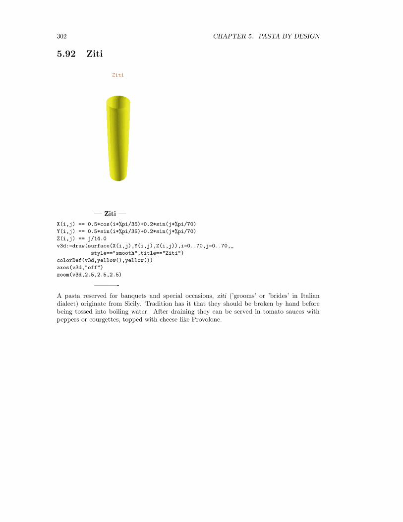
302 CHAPTER 5. PASTA BY DESIGN
5.92 Ziti
— Ziti —
X(i,j) == 0.5*cos(i*%pi/35)+0.2*sin(j*%pi/70)
Y(i,j) == 0.5*sin(i*%pi/35)+0.2*sin(j*%pi/70)
Z(i,j) == j/14.0
v3d:=draw(surface(X(i,j),Y(i,j),Z(i,j)),i=0..70,j=0..70,_
style=="smooth",title=="Ziti")
colorDef(v3d,yellow(),yellow())
axes(v3d,"off")
zoom(v3d,2.5,2.5,2.5)
———-
A pasta reserved for banquets and special occasions, ziti (’grooms’ or ’brides’ in Italiandialect) originate from Sicily. Tradition has it that they should be broken by hand beforebeing tossed into boiling water. After draining they can be served in tomato sauces withpeppers or courgettes, topped with cheese like Provolone.

Bibliography
[Lege11] George L. Legendre and Stefano Grazini. Pasta by Design. Thames and Hudson,2011, 978-0-500-51580-8.
[Segg93] David Henry von Seggern. CRC Standard Curves and Surfaces. CRC Press, 1993,0-8493-0196-3.
303

304 BIBLIOGRAPHY

Index
figures– CRCp26-2.1.1.1-3, 51– CRCp26-2.1.1.4-6, 52– CRCp26-2.1.2.1-3, 53– CRCp26-2.1.2.4-6, 54– CRCp28-2.1.3.1-6, 56– CRCp28-2.1.3.7-10, 57– CRCp28-2.1.4.1-6, 59– CRCp28-2.1.4.7-10, 60– CRCp30-2.2.1.1-3, 62– CRCp30-2.2.2.1-3, 63– CRCp30-2.2.3.1-3, 64– CRCp30-2.2.4.1-3, 65– CRCp30-2.2.5.1-3, 66– CRCp30-2.2.6.1-3, 67– CRCp32-2.2.10.1-3, 71– CRCp32-2.2.11.1-3, 72– CRCp32-2.2.12.1-3, 73– CRCp32-2.2.7.1-3, 68– CRCp32-2.2.8.1-3, 69– CRCp32-2.2.9.1-3, 70– CRCp34-2.2.13.1-3, 75– CRCp34-2.2.14.1-3, 77– CRCp34-2.2.15.1-3, 79– CRCp34-2.2.16.1-3, 81– CRCp34-2.2.17.1-3, 83– CRCp34-2.2.18.1-3, 85– CRCp36-2.2.19.1-3, 87– CRCp36-2.2.20.1-3, 89– CRCp36-2.2.21.1-3, 91– CRCp36-2.2.22.1-3, 93– CRCp36-2.2.23.1-3, 95– CRCp36-2.2.24.1-3, 97– CRCp38-2.2.25.1-3, 99– CRCp38-2.2.26.1-3, 101– CRCp38-2.2.27.1-3, 103– CRCp38-2.2.28.1-3, 105– CRCp38-2.2.29.1-3, 107– CRCp38-2.2.30.1-3, 109– CRCp40-2.2.31.1-3, 111– CRCp40-2.2.32.1-3, 113– CRCp40-2.2.33.1-3, 115– CRCp42-2.3.1.1-3, 117– CRCp42-2.3.2.1-3, 119
– CRCp42-2.3.3.1-3, 121– CRCp42-2.3.4.1-3, 123– CRCp44-2.3.5.1-3, 125– CRCp44-2.3.6.1-3, 127– CRCp44-2.3.7.1-3, 128– CRCp44-2.3.8.1-3, 129– CRCp46-2.4.1.1-3, 131– CRCp46-2.4.2.1-3, 133– CRCp46-2.4.3.1-3, 135– CRCp46-2.4.4.1-3, 137– CRCp48-2.4.5.1-3, 139– CRCp48-2.4.6.1-3, 141– CRCp48-2.4.7.1-3, 142– CRCp48-2.4.8.1-3, 143– CRCp50-2.5.1.1-3, 145– CRCp50-2.5.2.1-3, 147– CRCp50-2.5.3.1-3, 149– CRCp50-2.5.4.1-3, 151– CRCp50-2.5.5.1-3, 153– CRCp50-2.5.6.1-3, 154– CRCp52-2.6.1.1-3, 156– CRCp52-2.6.2.1-3, 158– CRCp52-2.6.3.1-3, 160– CRCp52-2.6.4.1-3, 162– CRCp52-2.6.5.1-3, 164– CRCp52-2.6.6.1-3, 165– CRCp54-2.7.1.1-3, 167– CRCp54-2.7.2.1-3, 169– CRCp54-2.7.3.1-3, 171– CRCp54-2.7.4.1-3, 173– CRCp54-2.7.5.1-3, 175– CRCp54-2.7.6.1-3, 176– CRCp56-2.8.1.1-3, 178– CRCp56-2.8.2.1-3, 180– CRCp56-2.8.3.1-3, 182– CRCp56-2.8.4.1-3, 184– CRCp56-2.8.5.1-3, 186– CRCp56-2.8.6.1-3, 187– CRCp58-2.9.1.1-3, 189– CRCp58-2.9.2.1-3, 190– CRCp58-2.9.3.1-3, 191– CRCp58-2.9.4.1-3, 193– CRCp58-2.9.5.1-3, 195– CRCp58-2.9.6.1-3, 197
305

306 Index
– CRCp60-2.9.10.1-3, 203– CRCp60-2.9.11.1-6, 205– CRCp60-2.9.7.1-3, 198– CRCp60-2.9.8.1-3, 199– CRCp60-2.9.9.1-3, 201