The 27-28 October 1986 FIRE IFO Cirrus Case Study: Cirrus ... · NASA-TM-113034 / e , The 27-28...
26
NASA-TM-113034 / e, The 27-28 October 1986 FIRE IFO Cirrus Case Study: Cirrus Parameter Relationships Derived from Satellite and Lidar Data PATRICK MINNIS , DAVID F. YOUNG , KENNETH SASSEN, JOSEPH M. fltLVAREZ AND CHRISTIAN J. GRUND Reprinted from MONTHLY WEATHER REVIEW, Vol. 118, No. 11, November 1990 American Meteorological Society https://ntrs.nasa.gov/search.jsp?R=19980026056 2018-05-27T05:06:40+00:00Z
Transcript of The 27-28 October 1986 FIRE IFO Cirrus Case Study: Cirrus ... · NASA-TM-113034 / e , The 27-28...
NASA-TM-113034 / e ,
The 27-28 October 1986 FIRE IFO Cirrus Case Study: Cirrus Parameter RelationshipsDerived from Satellite and Lidar Data
PATRICK MINNIS , DAVID F. YOUNG , KENNETH SASSEN,JOSEPH M. fltLVAREZ AND CHRISTIAN J. GRUND
Reprinted from MONTHLYWEATHERREVIEW, Vol. 118, No. 11, November 1990American Meteorological Society
https://ntrs.nasa.gov/search.jsp?R=19980026056 2018-05-27T05:06:40+00:00Z


Reprinted from MONTHLY WEATHER REVIEW, Vol. 118, No. 1 I, November 1990AmericanMeteorologicalSociety
The 27-28 October 1986 FIRE IFO Cirrus Case Study: Cirrus Parameter Relationships
Derived from Satellite and Lidar Data
PATRICK MINNIS*, DAVID F. YOUNG*, KENNETH SASSEN,**
JOSEPH M. ALVAREZ* AND CHRIST/AN J. GRUND ¢
*Atmospheric Sciences Division, NASA Langh'y Research Center, Hampton. Virginia,* Lockheed Engineering and Sciences Company, Hampton, Virginia,
* * Department o/Meteorology, University of Utah, Salt Lake City, Utah,*Department of Meteorology, University tf Wisconsin, Madison. Wisconsin
(Manuscript received 24 March 1989, in final form 12 June 1990)
ABSTRACT
Cirrus cloud radiative and physical characteristics are determined using a combination of ground-based,aircraft, and satellite measurements taken as part of the FIRE Cirrus Intensive Field Observations (IFO) during
October and November 1986. Lidar backscatter data are used with rawinsonde data to define cloud base, center,
and top heights and the corresponding temperatures. Coincident GOES 4-kin visible (0.65 _tm) and 8-km
infrared window ( 11.5 um) radiances are analyzed to determine cloud emittances and reflectances. Infrared
optical depth is computed from the emittance results. Visible optical depth is derived from reflectance using a
theoretical ice crystal scattering model and an empirical bidirectional reflectance model. No clouds with visible
optical depths greater than 5 or infrared optical depths less than 0.1 were used in the analysis.
Average cloud thickness ranged from 0.5 km to 8.0 km for the 71 scenes. Mean vertical beam emittances
derived from cloud-center temperatures were 0.62 for all scenes compared to 0.33 for the case study (27-28
October) reflecting the thinner clouds observed for the latter scenes. Relationships between cloud emittance,
extinction coefficients, and temperature for the case study are very similar to those derived from earlier surface-
based studies. The thicker clouds seen during the other IFO days yield different results. Emittances derivedusing cloud-top temperature were ratioed to those determined from cloud-center temperature. A nearly linear
relationship between these ratios and cloud-center temperature holds promise for determining actual cloud-top
temperatures and cloud thicknesses from visible and infrared radiance pairs.
The mean ratio of the visible scattering optical depth to the infrared absorption optical depth was 2.13 for
these data. This scattering efficiency ratio shows a significant dependence on cloud temperature. Values of mean
scattering efficiency as high as 2.6 suggest the presence of small ice particles at temperatures below 230 K. The
parameterization of visible reflectance in terms of cloud optical depth and clear-sky reflectance shows promise
as a simplified method for interpreting visible satellite data reflected from cirrus clouds. Large uncertainties in
the optical parameters due to cloud reflectance anisotropy and shading were found by analyzing data for various
solar zenith angles and for simultaneous AVHRR data. Inhomogeneities in the cloud fields result in uneven
cloud shading that apparently causes the occurrence of anomalously dark, cloudy pixels in the GOES data.These shading effects complicate the interpretation of the satellite data. The results highlight the need for
additional study of cirrus cloud scattering processes and remote sensing techniques.
I. Introduction
Accurate quantification of cirrus cloud propertiesfrom satellite measurements is particularly importantto the understanding of the role of cirrus in climatechange. The nonblackness of cirrus at thermal infraredwavelengths renders the interpretation of satellite datataken over cirrus more difficult than measurementsover most water clouds. The International Satellite
Cloud Climatology Project (ISCCP: see Schiffer andRossow 1983) is making an ambitious effort to derivedaytime cirrus coverage, altitudes, and optical depths
Corresponding author address: Patrick Minnis, Atmospheric Sci-
ences Division, NASA/Langley Research Center, Hampton, VA23665-5225.
over the globe during a 5-year period. The ISCCP anal-ysis algorithm (Rossow et al. 1988) relies entirely onbispectral data taken at visible (VIS: _0.65 #m) andinfrared (IR: _ 11.5 um) wavelengths. Although VIS-1R bispectral techniques have been suggested as feasiblemethods for determining bulk cirrus properties (e.g.,Shenk and Curran 1973; Reynolds and Vonder Haar1977), there has been very little application of thesetechniques to real data prior to the ISCCP.
The basic premise for using the bispectral approachis that the VIS extinction coefficient is related to the
IR absorption coefficient. This relationship implies thatthe cloud VIS reflectance may be used to infer thecloud's IR emittance. Having a value for the clear-skyIR radiance, it is possible to correct the observed cloudyradiance for cloud emittance resulting in an estimate

2403 MONTHLY WEATHER REVIEW VOLUMEII8
of the radiance emanating from a specified level in thecloud. The equivalent blackbody temperature of thislevel, usually the cloud center, is then converted tocloud altitude using a vertical sounding of temperature.The critical relationship required for this approach isthe dependence of IR emittance on VIS reflectancethrough the IR and VIS optical depths. Since cloudsscatter radiation anisotropically, this relationship is alsoinfluenced by the viewing and illumination conditions.
The ISCCP cirrus analysis (Rossow et al. 1988 ) uti-lizes a combination of theoretical and empirical modelsto determine the cloud visible optical depth from theobserved reflectance; the cloud emittance from the vis-ible optical depth; and finally, the cloud-top temper-ature from the cloud emittance and the observed in-frared radiance. The theoretical cloud model is a ra-
diative transfer scheme that simulates the scatteringand absorption of visible radiation by water dropletswith an effective radius of 10 #m. For water dropletsof this size, the ratio of VIS extinction to infrared ab-sorption optical depths is -_2.4. An analysis of coin-
cident satellite and lidar data by Platt et al. (1980) andtheoretical calculations employing cylinders (Piatt1979) suggest that this ratio is approximately equal to2.0 for cirrus. The ISCCP algorithm utilizes the lattervalue to provide a link between the water droplet modeland actual cirrus clouds.
Cirrus clouds are primarily composed of ice crystalswith various shapes having maximum dimensionsranging from about 20/_m to 2000 _m (e.g., Heyms-field and Platt 1984). The scattering properties of hex-agonal ice crystals differ considerably from sphericalparticles (Liou 1986). Because of the complexities in-volved in computing scattering by hexagonal solids,cylindrical columns have been used to approximatehexagonal crystals in radiative transfer calculations(e.g., Liou 1973). More recently, however, Takano andLiou (1989a) have solved the radiative transfer equa-tions for randomly oriented hexagonal plates and col-umns. Their results are the most realistic to date in
that they reproduce certain well-known cirrus opticalphenomena.
Absorption plays the dominant role in IR extinctionin cirrus clouds. Some theoretical investigations (Liouand Wittman 1979; Stephens 1980), however, haveshown that scattering effects may also be significant at
IR optical depths greater than t0. I. An IR radiancemeasured by a satellite over cirrus clouds, therefore, isthe product of both absorption and scattering processesin the cloud, as welt as the transmission of radiationfrom below the cloud (Platt and Stephens 1980). It isgenerally assumed, however, that scattering effects arenegligible so that the observed emittance is consideredto be the absorption beam emittance.
Empirical studies have also shed some light on theVIS reflectance-IR emittance relationship. Platt (1973)developed techniques for deriving cloud visible andinfrared properties from a ground-based lidar and an
upward-looking infrared radiometer. The backscatteredintensities measured with the lidar are used to define
cloud base and top heights. Cloud emittance was de-rived from the observed downwelling IR radiance. Plattand Dilley (1979) presented emittance results from aset of observations taken over Australia. Plattet al.
(1980) used lidar and satellite VIS-IR data to estimatethe dependence of beam emittance on VIS cloud re-flectance for a limited set of viewing and illuminationconditions over Colorado. Their results are more con-
sistent with theoretical scattering from ice cylinders
than with scattering from ice spheres. Aircraft radio-metric measurements taken over New Mexico (Pal-tridge and Platt 1981 ) have also been used to determinethe radiative characteristics of cirrus clouds as related
to the cloud ice water path. Those results provide fur-ther evidence that real clouds scatter more like cylindersthan spheres. Platt (1983) combined the results fromprevious studies and used them to explain the char-acteristics of two-dimensional bispectral histograms ofVIS-IR data observed from a geostationary satellite.Theoretical calculations of reflectance and emittance
for typical cirrus clouds were consistent with the sat-ellite data taken over areas of suspected cirrus clouds.While that study provided encouragement for using abispectral approach to retrieving cirrus properties frombispectral data, it also highlighted some of the diffi-culties that are likely to be encountered with such atechnique. Platt and Dilley (1984) used lidar and solarradiation measurements to measure part of the single-scattering phase function of real cirrus clouds. Theirresults fell within the range of laboratory measurementsand theoretical calculations for hexagonal crystals. Ananalysis of a large sample of ground-based lidar andinfrared data taken over Australia (Piatt et al. 1987)showed that the average emissivity of cirrus clouds isprimarily a function of the midcloud temperature.Though fraught with significant uncertainties, thatstudy also indicated that the theoretical value of theratio of visible extinction to infrared absorption forcirrus clouds may be too low.
From these previous studies, it appears that:
I ) cirrus cloud scattering properties are similar tothose of hexagonal crystals resulting in reflectance pat-terns that are unlike those from spheres;
2) scattering of IR radiation may be important indeterminations of IR optical depths; and
3 ) the ratio of VIS extinction to IR absorption coef-ficients is between --- 1.8 and 4.0.
The full impact of these results on using a VIS-IR bi-spectral mt.,i_od for retrieving cirrus properties is un-known. Differences between ice crystal and waterdroplet bidirectional reflectance patterns will introdt_eeerrors into the retrieved VIS optical depth. Use of anobserved beam emittance with a theoretical model that
assumes absorption only may affect the emittance es-timation. Finally, uncertainties in the extinction ratio

NOVEMBER1990 MINNIS, YOUNG, SASSEN, ALVAREZ AND GRUND 2404
(scattering efficiency) may cause significant errors inthe estimation of IR optical depth.
In this paper, the relationship between VIS reflec-tance and IR emittance is examined using data takenduring the First ISCCP Regional Experiment (FIRE)Cirrus Intensive Field Observations (IFO; see Starr
1987). Ground-based and aircraft lidars are used todefine the vertical locations of the cirrus clouds, while
satellites provide measurements of VIS and IR radi-ances. Both VIS and IR optical depths are computedfrom the reflectance and emittance data covering a
range of solar zenith angles missed in previous studies.These relationships are derived to provide a means forthe application ofa bispectral cirrus parameter retrievalalgorithm over the FIRE IFO region. Results are pre-sented for the entire IFO period with emphasis on 27-28 October 1986, the case study period. The data pre-sented here also constitute an initial source for devel-
oping cirrus bidirectional reflectance models and maybe used to help validate the models employed in the1SCCP algorithm.
2. Data
a. Lidar measurements
Lidar backscatter data were taken from four differentsources--three surface and one airborne. The lidars
and their operating systems and data products havebeen described elsewhere. Thus, only a brief descriptionof sources and their uses in this study are given here.
The University of Utah mobile polarization lidar(see Sassen et al. 1990) was located at Wausau, Wis-consin (WAU; 45.0°N, 89.7°W). The NASA Langley
ground lidar (Sassen et al. 1990) was situated at Ft.McCoy, Wisconsin (FMC; 43.9°N, 90.8°W), while theUniversity of Wisconsin High-Spectral Resolution LI-dar (Grund and Eloranta 1990) was in Madison, Wis-
consin (MAD; 43.1°N, 89.4°W). These ground sys-tems acquired nearly continuous lidar backscatter pro-files during the cirrus days of the IFO with especiallygood coverage during the case study period. The lidarreturns are used to define the cloud base and physicalthickness. Under conditions of small attenuation and
constant backscatter-phase function, the backscatterintensity profiles indicate the vertical distribution ofcloud extinction. A time series of these lidar returns
shown in Fig. 1 define the outlines of the cirrus cloudsas they passed over FMC during the afternoon of 28October. Solid black areas define the most intense cloud
backscatter. Grey denotes less backscatter and whiteindicates no cloud. Vertical stripes represent missing
data. Cloud-top altitude is fairly constant at _ 11 kin.Cloud base changes from _8 km to 10 km approxi-mately every half hour. In the morning, cloud base wasobserved at _7 kin, while cloud top varied between 8km and 11 kin. A similar variation is also seen in theWAU estimated volume backscatter coefficients shown
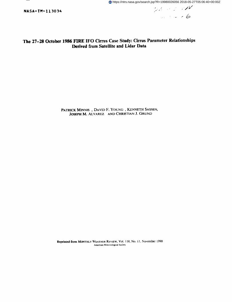
in Fig. 2 for the morning of 28 October. Darker portions
2oo I 12
87I 1 173 I
o. 160 1 10
1 33 I120_
_, o,lj Nog3F2
iosoQ2o_,_So,o; J
o 27L]
ooo_7i 1930 I i i2000 2030 21100 21130 22001900
UTC
FIG. 1. Lidar backscatter ratios from cirrus clouds passing over
Ft. McCoy during 28 October 1986.
of the plot correspond to higher backscatter coefficientvalues. The particle backscattering efficiency dependson cloud particle shape and phase. Further details ofthe lidar returns are reported in the cited references.
Three parameters are derived from plots like thosein Figs. 1 and 2 by averaging the data within + 15 rainof the UTC (Coordinated Universal Time) half hourplus 5 rain. All times, however, will be given here tothe nearest half hour. Cloud-top altitude, zt, and cloud-base altitude, zb, are defined as the average altitudesof the highest and lowest nonclear-air backscatter re-turns, respectively. Similarly, the cloud thickness is h= zt - zb. Mean cloud height (approximately cloudcenter height), Zc, is the backscatter-intensity weightedaverage height of the cloud. It corresponds roughly tothe altitude below which 50% of the lidar backscatter
is accumulated. These parameters were estimated
graphically for the FMC and WAU sites, while a com-puter analysis was applied to the MAD results. Thevalue of z_ for MAD corresponds to the midpoint inoptical thickness independent of cloud attenuation (seeGrund and Eloranta 1990). Since the clouds are ad-
vecting over the fixed surface sites, the averaged lidardata correspond to a thin vertical cross section takenout of some cloud volume. It is assumed that the cross-
section-averaged data represent the mean conditionsof that volume.
These same parameters were also derived from thedown-looking lidar backscatter plots reported by Spin-hirne et al. ( 1988 ) for selected flight tracks of the high-flying, NASA ER-2 aircraft over the IFO area. Shortertime averages were used since the plane's motion
greatly increased the cirrus advection rates relative tothe lidar. In some instances, the clouds were too thickfor complete penetration by the ground-based lidars.To determine these occurrences, the cloud altitudes
estimated from the ground were compared to thosedetermined from the nearest aircraft flight. On most
days, there was good agreement between the surfaceand airborne lidars. The thick clouds observed on 22October required use of the aircraft lidar to estimatez,. At other times when no aircraft data were availablefor comparison, a different approach was used to es-timate zt (see section 3a).
2405 MONTHLYWEATHERREVIEW VOLUMEII8
12
• -.---. .. ig_. :
/ • ,: -_=:-=._:-=,-_ _"._a_÷ _--=, '_
s -1 ....... __-;t_ ....
5 1 , I I I I l I
1500 1600 1700 1800UTC
FIG. 2. Estimated lidar volume extinction efftcienciesfrom cirrus clouds over WAU 28 October 1986.
-10
-1.5
..-?..P........
-2.5
-30
-35
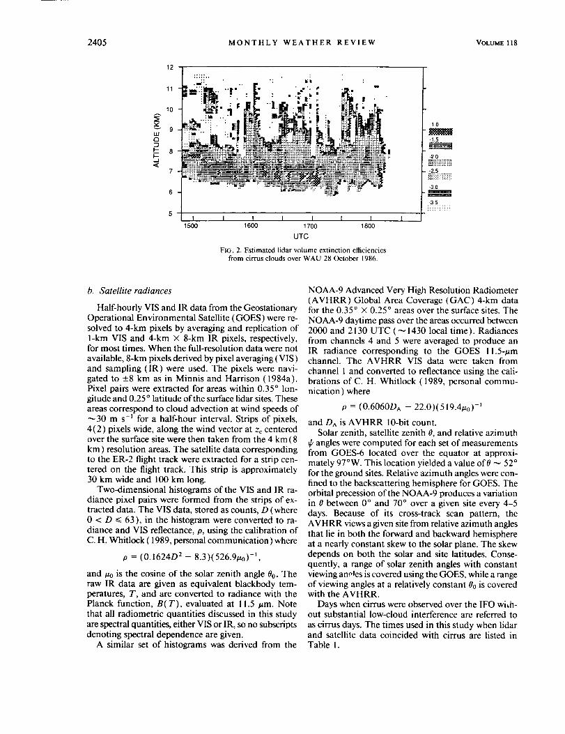
b. Satellite radiances
Half-hourly VIS and IR data from the GeostationaryOperational Environmental Satellite (GOES) were re-solved to 4-km pixels by averaging and replication ofl-km VIS and 4-km × 8-km IR pixels, respectively,for most times. When the full-resolution data were not
available, 8-km pixels derived by pixel averaging (VIS)and sampling (IR) were used. The pixels were navi-gated to _+8 km as in Minnis and Harrison (1984a).Pixel pairs were extracted for areas within 0.35 ° lon-gitude and 0.25 ° latitude of the surface lidar sites. Theseareas correspond to cloud advection at wind speeds of_30 m s -_ for a half-hour interval. Strips of pixels,
4(2) pixels wide, along the wind vector at z_ centeredover the surface site were then taken from the 4 km ( 8kin) resolution areas. The satellite data correspondingto the ER-2 flight track were extracted for a strip cen-tered on the flight track. This strip is approximately30 km wide and 100 km long.
Two-dimensional histograms of the VIS and IR ra-diance pixel pairs were formed from the strips of ex-tracted data. The VIS data, stored as counts, D (where0 < D _< 63), in the histogram were converted to ra-
diance and VIS reflectance, p, using the calibration ofC. H. Whitlock ( 1989, personal communication) where
= (0.1624D 2 - 8.3)(526.9_0) -_,
and uo is the cosine of the solar zenith angle 00. Theraw IR data are given as equivalent blackbody tem-peratures, T, and are converted to radiance with thePlanck function, B(T), evaluated at 11.5 vm. Notethat all radiometric quantities discussed in this studyare spectral quantities, either VIS or IR, so no subscriptsdenoting spectral dependence are given.
A similar set of histograms was derived from the
NOAA-9 Advanced Very High Resolution Radiometer(AVHRR) Global Area Coverage (GAC) 4-km datafor the 0.35 ° × 0.25 ° areas over the surface sites. The
NOAA-9 daytime pass over the areas occurred between2000 and 2130 UTC ( --- 1430 local time). Radiancesfrom channels 4 and 5 were averaged to produce anIR radiance corresponding to the GOES l l.5-#mchannel. The AVHRR VIS data were taken from
channel 1 and converted to reflectance using the cali-brations of C. H. Whitlock (1989, personal commu-nication ) where
p = (0.6060DA - 22.0)(519.4#0) -l
and DA is AVHRR 10-bit count.Solar zenith, satellite zenith O, and relative azimuthangles were computed for each set of measurements
from GOES-6 located over the equator at approxi-mately 97°W. This location yielded a value of 0 _ 52 °for the ground sites. Relative azimuth angles were con-fined to the backscattering hemisphere for GOES. Theorbital precession of the NOAA-9 produces a variationin 0 between 0 ° and 70 ° over a given site every 4-5days. Because of its cross-track scan pattern, the
AVHRR views a given site from relative azimuth anglesthat lie in both the forward and backward hemisphereat a nearly constant skew to the solar plane. The skewdepends on both the solar and site latitudes. Conse-quently, a range of solar zenith angles with constantviewing an_,les is covered using the GOES, while a rangeof viewing angles at a relatively constant O0 is coveredwith the AVHRR.
Days when cirrus were observed over the IFO with-out substantial low-cloud interference are referred to
as cirrus days. The times used in this study when lidarand satellite data coincided with cirrus are listed inTable I.
NOVEMBER 1990 MINNIS, YOUNG, SASSEN, ALVAREZ AND GRUND 2406
TABLE I. Times and locations of lidar-satellite data
used in this study.
Site Day Month Times (UTC)
FMC 22 October 1300, 1330, 1400, 1600, 1630, 1700,2000
27 2030, 210028 1330, 1400, 1430, 1500, 1600, 1700,
19001930, 2000, 2030, 2100, 2130, 2200
30 2000, 20301 November 1800, 19002 1900, 2000, 2100
MAD 28 October 1330, 1500, 1600, 1700, 1800, 1930,20O0
2030, 2100, 2130, 2200
WAU 22 October 1300, 1330, 1400, 1430, 1600, 1630,1700, 1800
1830, 1900, 1930, 2130, 220028 1500, 1600, 1700, 1800, 1900, 1930,
2000. 20302100, 2130
30 2130, 22001 November 1800, 1900, 20002 1700, 1800, 1900, 2000, 2100
c. Temperature data
Soundings from Green Bay, Wisconsin, determined
the temperature-height relationships for all of the data.
Linear interpolation was used to estimate half-hourly
soundings from the six-hourly data. Cloud-top tem-
perature, Tt, corresponds to zt on the soundings. Mean
cloud temperature, To, is found from Zc. Surface tem-
peratures taken every six hours at MAD, WAU, and
Lone Rock, Wisconsin (Hahn et al. 1988), and oc-
casionally at the FMC site, were used to supplement
the clear-sky temperatures derived from the satellite
data as described below.
The clear-sky temperature, Ts, is the equivalent
blackbody temperature for clear scenes. It is estimated
in several different ways. The first order estimate is
taken from the initial results of Minnis et al. (1990),
which applies the techniques of Minnis et ai. (1987)
to 0.5 ° regions within the greater IFO area. That ap-
proach sets a VIS threshold _2 counts above the clear-
sky count, Ds (see section 3). All pixels considered to
be clear must be darker than this threshold and have
a temperature that is no more than 3 K colder than
the maximum observed temperature. The 4 K range
for clear pixels, roughly double the typical value over
Wisconsin land areas, allows for shading effects in
partly cloudy scenes. The average temperature of the
clear pixels is the initial value of Ts. Surface air tem-
peratures, Tg, are also taken from nearby ground sta-
tions. A rough correction is applied to these tempera-
tures to adjust for atmospheric attenuation and the
difference between the temperature of the surface skin
and the air at shelter height. The resulting estimate of
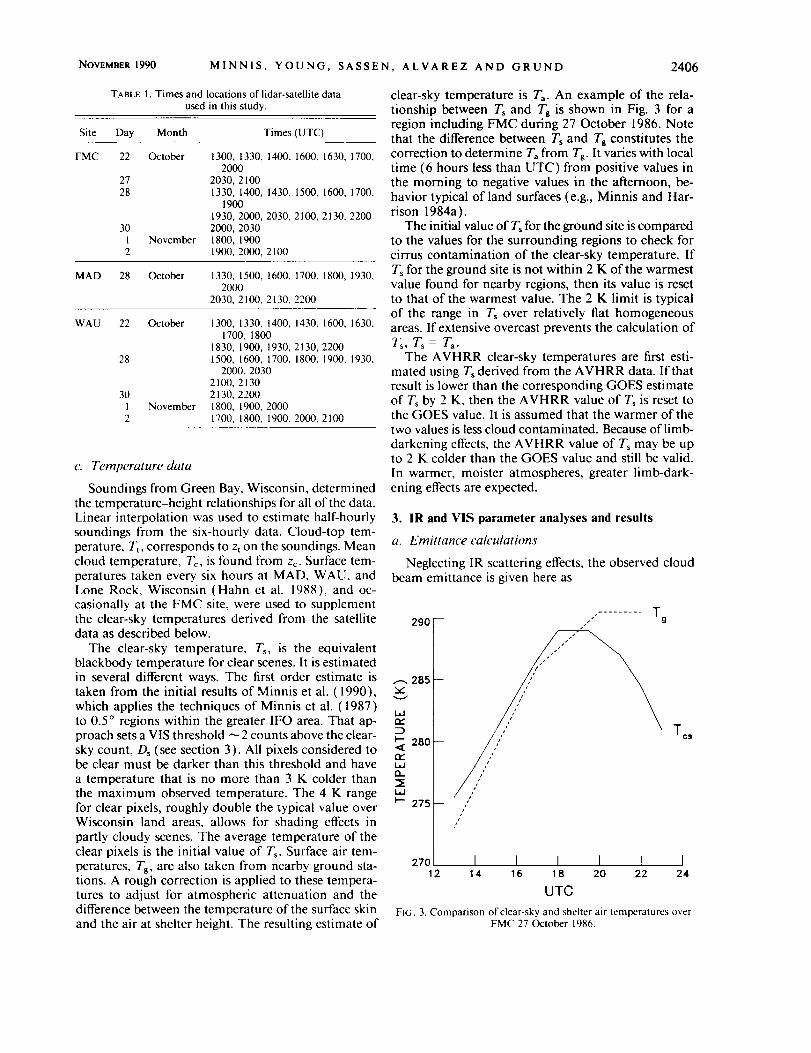
clear-sky temperature is Ta. An example of the rela-
tionship between T_ and Tg is shown in Fig. 3 for a
region including FMC during 27 October 1986. Note
that the difference between Ts and Tg constitutes the
correction to determine Ta from Tg. It varies with local
time (6 hours less than UTC) from positive values in
the morning to negative values in the afternoon, be-
havior typical of land surfaces (e.g., Minnis and Har-
rison 1984a).
The initial value of Ts for the ground site is compared
to the values for the surrounding regions to check for
cirrus contamination of the clear-sky temperature. If
T_ for the ground site is not within 2 K of the warmest
value found for nearby regions, then its value is reset
to that of the warmest value. The 2 K limit is typical
of the range in T_ over relatively flat homogeneous
areas. If extensive overcast prevents the calculation of
Ts, Ts=Ta.
The AVHRR clear-sky temperatures are first esti-
mated using T_ derived from the AVHRR data. If that
result is lower than the corresponding GOES estimate
of Ts by 2 K, then the AVHRR value of T_ is reset tothe GOES value. It is assumed that the warmer of the
two values is less cloud contaminated. Because of limb-
darkening effects, the AVHRR value of Ts may be up
to 2 K colder than the GOES value and still be valid.
In warmer, moister atmospheres, greater limb-dark-
ening effects are expected.
3. IR and VIS parameter analyses and results
a. Emittance calculations
Neglecting IR scattering effects, the observed cloud
beam emittance is given here as
290• ......... T
/
I
/
/
Xcs
.--., 285 --v
280-.<_cv.
EL
laJ
I-- 275-
270 I I I I I I12 14 16 18 20 22 24
UTC
FIG. 3. Comparison of clear-sky and shelter air temperatures overFMC 27 October 1986.

2407 MONTHLY WEATHER REVIEW VOLUMEII8
_b(0) = [B(T)- B(Ts)][B(Tz) - B(Ts)]-', (1)
where Tz is the temperature at some altitude z corre-sponding to the cloud. The mean clear-sky equivalentblackbody temperature over the area of interest, Ts,has a weak dependence on 0.
Cloud beam emittance is calculated twice for each
set of lidar-radiance data using Tz = Tc and Tz = Tt.The former value, which corresponds to the quantityused in most previous studies (e.g., Platt et al. 1980),may be more representative of the actual radiating partof the cloud. It does not necessarily correspond to thecenter of the cloud. The actual cloud-top temperaturedefines the vertical limit of the cloud. Emittances are
computed using both temperatures to determine ifthere is a relationship between them that may be usedto better define the physical boundaries of the cloudfrom the satellite data.
Due to angular effects, the values of Tc may requiresome adjustment from the initial lidar values. It is un-likely that a value ofeb = 1 will be measured at a usefulsatellite zenith angle using Tt because of the low densityof particles in the upper portions of the cloud. On theother hand, _b(Tc) may be greater than one for somethick cirrus clouds. Although emittances greater thanunity may be possible due to scattering enhancementsof the upward radiance (Platt and Stephens 1980), theuncertainties in zc for thick clouds preclude any defin-itive measurements of eb > I. Thus, if eb > 1, Tc is
decreased until the average value of eb for a given re-flectance is less than or equal to one. While this limitis reasonable, it is somewhat arbitrary resulting in in-creased uncertainty in the true value of Tc for thickclouds.
During initial processing of the data, it was deter-mined that the maximum emittance found using Ttwas _0.86, except for those cases with cloud cover toodense for complete penetration of the lidar beam. Toidentify and correct the exceptions, a new estimate ofTt was computed whenever Tc was adjusted as ex-plained above. This new estimate, T't, is determinedfrom the following formula, which forces the cloud tohave the maximum observed emittance:
B(T't) = [B(T) - O.14B(Ts)]/0.86.
The resulting value was then compared to Tt. If T't< Tt - 3 K, then Tt is reset to T't. The 3 K allowance(_0.5 km) is made to account for uncertainties in thelidar-determined cloud-top, due to time averaging andunknown penetration depth in thicker cloud. The result
was then compared to the tropopause temperature us-ing the assumptions that the cloud occurs in the tro-posphere and the tropopause temperature is the coldestin the troposphere. If Tt is colder, it is reset to equalthe tropopause temperature. The value of zt was thenadjusted to correspond to the final value of Tt.
It is also assumed that
% = 1 -- exp(--_'e/_t), (2)
where re is the IR absorption optical depth and= cos0. Based on the results of Platt and Stephens(1980), it is expected that the viewing zenith angledependence of _bwill not depart significantly from (2).Values of beam emittance derived with AVHRR data
may be adjusted to the GOES viewing zenith anglewith this relationship.
The vertical emittance from (2) is
_a = 1 - exp(-ze). (3)
It is assumed here that scattering effects are negligiblein the upwelling direction. Thus, re is equivalent tothe IR absorption optical depth and _a is equal to thevertical emittance.
b. VIS reflectance and optical depth calculations
Values of clear-sky reflectance m and clear-sky countD, were computed for each region using the 0.01 o clear-sky albedo, a_, map of the IFO area (42°N-47°N,87°W-92°W) constructed by Minnis et al. (1990) fromGOES data at each half hour. Clear-sky reflectance overany latitude ?_and longitude _ of the grid at time t, isestimated as
re(X, 4_, t, 0o, 0, _) = _s(X, O, t, Oo)Xs(Oo, O, _), (4)
where ×s is the anisotropic reflectance factor with valuesgiven by the model of Minnis and Harrison (1984b).Ds was determined by p_ using the VIS calibrations.The value of 0o varies by a few degrees over the IFOtime period, while the values of as were normalized to
a single value of solar zenith angle designated 0o,. Toaccount for these variations, as(t, 0o) = as(t,
00)uo//_o,, where _0_ = cos0o,. The clear-sky diffuse al-bedo is
a :f.s(Oo),,oa.o/f,,oa.o,integrated over Uo = 0, 1. The value of a_ is set equalto as(57 °) in this study since the full range of solarzenith angles is not observed at the time and latitudeof the IFO, the true value of a_ is usually equivalentto as measured at 0o _ 53 °, and 57 ° is the lowestobserved 0o for this dataset.
Cloud reflectance, pc, is estimated with a variant ofthe simple physical model used by Platt et al. (1980).That is,
p =TaPc + psTcTu + Cqd(1 -- Old)(1 -- Tc - C_c), (5)
where p is the measured reflectance, ac is the cloudalbedo at 0o, ×c is the anisotropic reflectance factor forthe cloud .... d p_ = a_xc(Oo, O, _/).
This model assumes that all ozone absorption occursabove the cloud (first term ) and all Raylelgh and aero-sol scattering is confined to the layers below the cloud.The second term in (5) accounts for direct solar ra-diation, which passes through the cloud, reflects fromthe surface, and passes back through the cloud in the

NOVEMBER1990 MINNIS, YOUNG, SASSEN, ALVAREZ AND GRUND 2408
direction of the satellite. The third term accounts for
the radiation that passes down through the cloud viamultiple scattering, reflects diffusely from the surfacebelow the cloud, and returns through the cloud scat-tered in the direction of the satellite.
Using the parameterization of Rossow et al. ( 1988 ),the transmittance of the air above the cloud is
T, = exp[-u(0.085 - 0.00052u)(1/_0 + 1/_)],
where u is the ozone abundance in cm-STP. The valueused here, it = 0.32 cm-STP, is the average of the mid-latitude winter and summer standard atmospheres
above 10 km from McClatchey et al. (1973). Platt etal. (1980) implicitly assumed that Ta = 1. The currentmodel accounts for ozone absorption in the Chappiusbands.
The transmittance of the cloud to direct solar radia-
tion at Oo is
Tc = exp(-r,,/2/_o), (6)
(see Platt et al. 1980). Similarly, the direct transmit-tance from the surface through the cloud along thesatellite line of sight is
Tu = exp(-rv/2/_).
The visible optical depth is reduced by a factor of twofor the direct transmittance because at least half of the
radiation scattered out of the beam is actually diffractedin the forward direction (Takano and Liou 1989a).Clear-sky reflectance along the satellite line of sight isPs and _a is the effective clear-sky albedo to diffuse
radiation directly below the cloud. Due to the relativehomogeneity of clear-sky reflectance over the IFO re-gion, it is assumed that c_a and ps may be computedfrom the same data. The albedo of the cloud to diffuse
radiation is ad.In addition to values for the clear-sky terms, the so-
lution of (5) for Pc requires specification of r v and Xc.VIS optical depth is estimated by iteration on ( 5 ) usinga linear interpolation of the relationships between _oand _c for randomly oriented hexagonal columns(length, 125 urn; width, 50 tzm) in Fig. 4 of Takanoand Liou (1989b). Similar interpolations are used toestimate O_d(_'v), where
;o' /fo'ad(rv) = c_a(rv, #0)de0 /_0d#0.
For a given measurement, (5) is solved iteratively usingan initial guess of cloud albedo such that Tc = T, = 1- c_c. A value for z_ is determined from this initial
guess using the theoretical data. A limit of 20 iterationsis imposed to achieve an absolute difference of less than0.001 between the guess and the computed value ofac. Generally, fewer than five iterations are required.Since O_cmust be greater than zero, ac is set to 0.001for initial guesses that are less than or equal to zero. Ifr,. < 0, c_o < 0.001, or c_c_< 0.001 after any iteration,
it is assumed that rv is indeterminate and the data arenot used. The causes for these indeterminate cases (e.g.,
shadowing of the surface by adjacent clouds or inad-equate specification of the cloud reflectance anisotropy)are discussed later.
A value for ×c, which depends on rv and the cloudmicrophysics, is needed to determine C_cfrom p_. Nomodels of Xc are currently available for ice clouds interms of z_. Because of favorable angles Platt et al.(1980) were able to assume that ×c = I. However, mostempirical and theoretical bidirectional reflectancemodels for cloudy scenes (e.g., Suttles et al. 1988) reveala systematic decrease in ×c with 00 for the angles usedin this study. The cloudy scene bidirectional reflectancemodel developed by Minnis and Harrison (1984b) isused initially to estimate xc. That model's reflectanceanisotropy is similar to other empirical and theoreticalmodels (Stuhlmann et al. 1985). The inclusion of all
cloud types in its derivation should produce a reflec-tance pattern that combines the scattering propertiesof both ice and liquid water clouds. New values of ×c,derived after the initial analysis, are used to reanalyzethe data to provide better estimates of VIS opticaldepth.
The data were preprocessed to define limits to elim-inate pixels containing low clouds and those scenescontaining only thick clouds. Underlying low cloudsconfuse the interpretation of cirrus radiances. Thickclouds increase the uncertainty in the determinationof To, Tt, and _b. A simple filter of the form,
_b = 1 -- exp(-kad_), (7)
where k is a regression coefficient, was used to eliminate
low clouds. This formula gives a first approximationto the relationship between _b and cloud albedo. Therationale for its use and the details of the filtering aredescribed in appendix A. The data were also screenedfor partially cloud-filled pixels as detailed in appen-dix B.
c. Results and discussion for rnidcloud temperatureemittances
All results discussed in this section are based on T_= T¢ in ( 1 ). Examples of the two-dimensional GOEShistograms used in this analysis are shown in Figs. 4aand 4b for 1500 UTC over FMC. The latter representsa cirrus case (see Fig. 1) on 28 October, while theformer, taken during the previous day, is typical ofclear conditions. Maximum clear-sky reflectance forthis hour is denoted with the dashed line in Fig. 4a.Some of the cold, apparently cloudy pixels in Fig. 4b
are no brighter than the clear pixels in Fig. 4a. More-over, some of these pixels are actually darker than thecloud-free pixels. Depending on Xc and rv, some of thecold, dim pixels yield a positive value of c_c in the so-lution of(5 ). Those pixels with indeterminate _'_ andT < Ts - 3 K are hereafter referred to as "dark" pixels.

2409 MONTHLY WEATHER REVIEW VOLUMEII8
20
I.-z:2)0015
I.d_J
10
4 3
5 2
2
27
25
2
I I 1 I282 281 280 279
11.5 /zm TEMPERATURE (K)
FIG. 4a. VIS-IR histogram of GOES pixels over FMC at 1500UTC 27 October 1986 (numbers denote frequency of occurrence oftemperature-count pairs).
They are not used to solve (7). Their impact and originsare discussed in section 4d. The cloud emittances
are plotted in Fig. 5a against the measured reflectancesfor the case in Fig. 4b. Eliminating the dark pixels andapplying (5) to the data in Fig. 5a yields the cloudalbedo values. Averaging the emittances for a givenalbedo produces the mean values and the standard de-viations plotted in Fig. 5b. The solid line representsthe solution to (7) using the average value of k = 5.1.The mean beam emittance and VIS optical depths for
the data used in Fig. 5b are gb = 0.38 and _v = 0.59.The data from FMC in Fig. 5b for this hour are
compared to those from MAD and WAU shown in
Fig. 6. Apparently, the clouds over WAU are muchdenser than those over MAD, while the MAD obser-vations are similar to those over FMC. Values of Tc
differed by only 1 K among the sites, while Tt rangedfrom 225 K at WAU to 217 K at MAD. Depolarizationratios derived from the lidar returns indicated inter-
mittent liquid layers during the morning of 28 October,especially at _ 1500 UTC. Those liquid layers may bethe source of the larger emittances over WAU. Datafrom all three sites were combined, averaged, and fitwith (7) yielding k = 5.6. The scatter in the meansbetween the sites at a given hour is of the same orderas that for different hours at the same site as seen in
Fig. 7 for FMC at 3 times during 28 October.
1) GOES-SURFACE LIDAR RESULTS
A summary of the results for the case study 27-28October is given in Table 2. Cloud-top heights rangefrom 9.5 to 11.0 km at all three sites. The cloud-center
temperatures vary by about 25 K. Cloud optical depthswere much greater over WAU than over the other sites.Dark pixels were found more often over FMC andMAD than over WAU.
Due to dropouts, the only data available for 1500UTC during the primary IFO cirrus days occurred on28 October. Data from other days were available formost of the afternoon hours. The combined datasets
permitted coverage of the full range of emittances at agiven hour as illustrated in Fig. 8 for 2000 UTC. Datafor all of the hours used in the case study and the entireIFO analyses are shown in Figs. 9a and 9b, respectively.The clouds over the area during 27-28 October weregenerally thinner with lower emittances than most ofthose observed during the other days. The combined
datasets (Fig. 9b) yield a large number of samples for_b < 0.5 and eb > 0.8 and relatively few for intermediatevalues of _b. Apparently, the cirrus, which occurredduring the IFO, tended to be either very thick or rel-
z
0
1
1
2 1 t t 2
2 1 1 l 2 I
1 1
l 1 t 1
t I 1 1 I
1 t I I
] I 2 2 2 I I
1 i i
4 _ 1 z
] 2 1 I
I I 2
t
1°1_-I 1 I I I I I I I I I I I
:ZT_ 21'? 275 27') 271 _69 267 265 26] 26t 2S9 _!S7 2S_
11.5 _m TEMPERATURE (K)
FIG. 4b. VIS-IR histogram of GOES pixels over FMC at 1500 UTC 28 October 1986.Dashed line refers to maximum clear-sky count.
I253

NOVEMBER 1990 MINNIS, YOUNG, SASSEN, ALVAREZ AND GRUND 2410
1.0 "
0.8-
I..U
¢_ .t..i.4-..t-
'_ 4-4-4-4- 4-
_ i..÷+41
4-',, +4. 4.U.I_÷ ÷
0 o,4- :+++++0. +_:*+
I
0 ,**0,2- , 4.+
J 4.4.:+% 4-I
0.0 ' II I , I i I i I * I
0,0 0.2 0.4 0.6 0.8 1.0
VISIBLE REFLECTANCE
FIG. 5a. Cloud emittances and observed reflcctances for T < 7",
- 3 K derived from Fig. 4b. Dashed line refers to maximum clear-
sky reflectance.
WOz<
W
O_.J¢,.)
1.0
0.8
0.6
0.4
0.2
+4-
4- 4-
0
0[]
O
OoDrlD
[]
+ WAUSAU
O FT. MCCOY
[] MADISON
0.0 , I I I i I , I I I
0.0 0.2 0.4 0.6 0.8 1.0
CLOUD ALBEDO
FIG. 6. Average cloud emittance versus cloud albedo at 1500 UTC28 October 1986 over three sites from GOES VIS-IR data.
atively thin. Perhaps, a longer time period would pro-duce more uniform sampling. No data are found for_b < 0.08 since no clouds are recognized if T > Ts-3K.
Table 3 summarizes the values of z_ derived fromall of the GOES-surface IFO data (Fig. 9b) and fromcase study data only (Fig. 9a) for each relevant time.The average scattering angles, O, between the sun, sat-
ellite, and scene are also listed in Table 3. Visible optical
depths observed during the case study are less than halfof those observed for all of the IFO cirrus days.
The mean vertical emittance is given as a function
of temperature in Fig. 10. The dashed line correspond-ing to the results from Fig. 7a of Platt et al. (1987) isincluded for comparison. Although there is a generalincrease in _a with increasing cloud temperature, the
1.0
LidOZ
I-
W
£3
O._J(,3
0.8
0.6
T
0.4 I
/0.0
0.0
I
0.2
. I , I i
0.4 0.6
CLOUD ALBEDO
I , I
0.8 1.0
FIG. 5b. Cloud albedos and mean cloud emittances derived from
Fig. 5a without "dark" pixels. Vertical lines represent standard de-
viations. The curved line denotes the regression fit to Eq. (7).
IiiOz
LU
r7
O_JO
1.0
0.8
0.6
0.4
0.2 []
D
+
4-%
o0- o-O
CD o
4-[]
+
+[]
[][]
4-
O[]
1600 UTC1930 UTC
2100 UTC
0.0 i I , I l I i I • I
0.0 0.2 0.4 0.6 0.8 1.0
CLOUD ALBEDO
FIG. 7. Average cloud emiltance and albedo at three times during28 October 1986 over FMC from GOES VIS-IR data.
2411 MONTHLY WEATHER REVIEW VOLUME II8
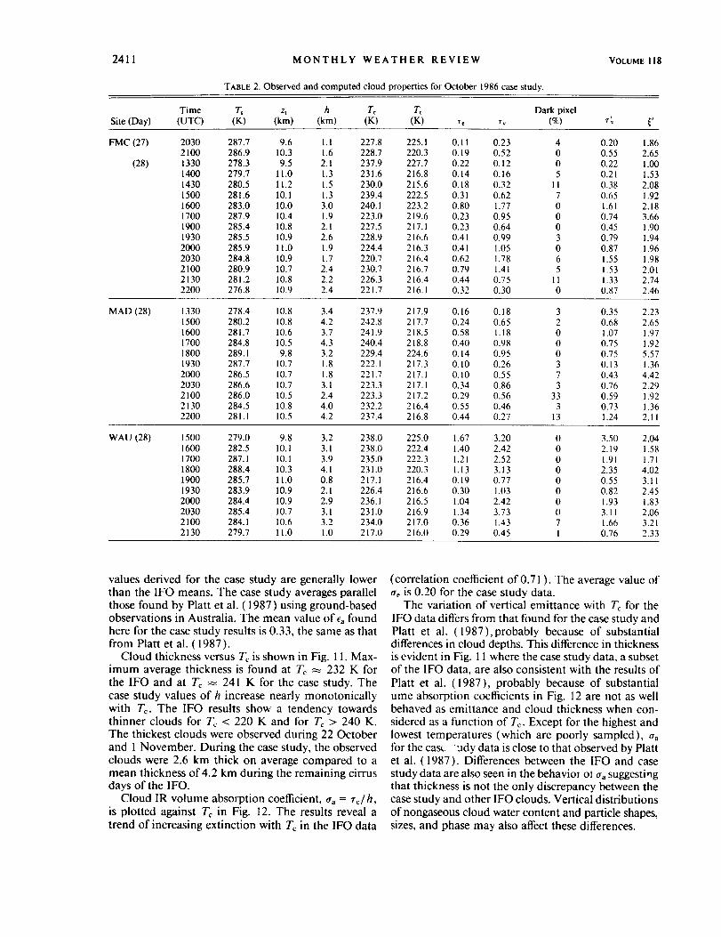
TABLE 2. Observed and computed cloud properties for October 1986 case study.
Time 7", z, h T¢ Tt Dark pixelSite (Day) (UTC) (K) (km) (km) (K) (K) re rv (%) r'v _'
FMC (27)
(28)
2030 287.7 9.6 1.1 227.8 225.1 0. l 1 0.23 4 0.20 1.862100 286.9 10.3 1.6 228.7 220.3 0.19 0.52 0 0.55 2.651330 278.3 9.5 2.1 237.9 227.7 0.22 0.12 0 0.22 1.001400 279.7 11.0 1.3 231.6 216.8 0.14 0.16 5 0.21 1.531430 280.5 11.2 1.5 230.0 215.6 0.18 0.32 11 0.38 2.08
1500 281.6 10.1 1.3 239.4 222.5 0.31 0.62 7 0.65 1.921600 283.0 10.0 3.0 240.1 223.2 0.80 1.77 0 1.61 2.181700 287.9 10.4 1.9 223.0 219.6 0.23 0.95 0 0.74 3.661900 285.4 10.8 2.1 227.5 217.1 0.23 0.64 0 0.45 1.901930 285.5 10.9 2.6 228.9 216.6 0.41 0.99 3 0.79 1.942000 285.9 11.0 1.9 224.4 216.3 0.41 1.05 0 0.87 1.962030 284.8 10.9 1.7 220.7 216.4 0.62 1.78 6 1.55 1.982100 280.9 10.7 2.4 230.7 216.7 0.79 1.41 5 1.53 2.012130 281.2 10.8 2.2 226.3 216.4 0.44 0.75 11 1.33 2.742200 276.8 10.9 2.4 221.7 216.1 0.32 0.30 0 0.87 2.46
MAD (28) 1330 278.4 10.8 3.4 237.9 217.9 0.16 0.18 3 0.35 2.231500 280.2 10.8 4.2 242.8 217.7 0.24 0.65 2 0.68 2.651600 281.7 10.6 3.7 241.9 218.5 0.58 1.18 0 1.07 1.971700 284.8 10.5 4.3 240.4 218.8 0.40 0.98 0 0.75 1.921800 289.1 9.8 3.2 229.4 224.6 0.14 0.95 0 0.75 5.571930 287.7 10.7 1.8 222. t 217.3 0.10 0.26 3 0.13 1.362000 286.5 10.7 1.8 221.7 217.1 0.10 0.55 7 0.43 4.422030 286.6 10.7 3.1 223.3 217.1 0.34 0.86 3 0.76 2.292100 286.0 10.5 2.4 223.3 217.2 0.29 0.56 33 0.59 1.922130 284.5 10.8 4.0 232.2 216.4 0.55 0.46 3 0.73 1.362200 281.1 10.5 4.2 237.4 216.8 0.44 0.27 13 1.24 2.11
WAU (28) 1500 279.0 9.8 3.2 238.0 225.0 1.67 3.20 0 3.50 2.041600 282.5 10.1 3.1 238.0 222.4 1.40 2.42 0 2.19 1.581700 287.1 10. t 3.9 235.0 222.3 1.21 2.52 0 1.91 1.711800 288.4 10.3 4.1 231.0 220.3 1.13 3.13 0 2.35 4.021900 285.7 11.0 0.8 217.1 216.4 0.19 0.77 0 0.55 3.111930 283.9 10.9 2.1 226.4 216.6 0.30 1.03 0 0.82 2.452000 284.4 10.9 2.9 236.1 216.5 1.04 2.42 0 1.93 1.832030 285.4 10.7 3.1 231.0 216.9 1.34 3.73 0 3.11 2.062100 284.1 10.6 3.2 234.0 217.0 0.36 1.43 7 1.66 3.212130 279.7 11.0 1.0 217.0 216.0 0.29 0.45 1 0.76 2.33
values derived for the case study are generally lower
than the IFO means. The case study averages parallel
those found by Platt et al. (1987) using ground-based
observations in Australia. The mean value of e, found
here for the case study results is 0.33, the same as that
from Platt et al. (1987).
Cloud thickness versus Tc is shown in Fig. 1 1. Max-
imum average thickness is found at Tc _ 232 K for
the IFO and at Tc _ 241 K for the case study. The
case study values of h increase nearly monotonically
with T_. The IFO results show a tendency towards
thinner clouds for Tc < 220 K and for Tc > 240 K.
The thickest clouds were observed during 22 October
and 1 November. During the case study, the observed
clouds were 2.6 km thick on average compared to a
mean thickness of 4.2 km during the remaining cirrus
days of the IFO.
Cloud IR volume absorption coefficient, aa = re�h,
is plotted against Tc in Fig. 12. The results reveal a
trend of increasing extinction with Tc in the IFO data
(correlation coefficient of 0.71 ). The average value of
a_ is 0.20 for the case study data.
The variation of vertical emittance with Tc for the
IFO data differs from that found for the case study and
Platt et al. (1987),probably because of substantial
differences in cloud depths. This difference in thickness
is evident in Fig. 1 1 where the case study data, a subset
of the 1FO data, are also consistent with the results of
Platt et al. (1987), probably because of substantial
ume absorption coefficients in Fig. 12 are not as wellbehaved as emittance and cloud thickness when con-
sidered as a function of T_. Except for the highest and
lowest temperatures (which are poorly sampled), aa
for the cas_ 'udy data is close to that observed by Platt
et al. (1987). Differences between the IFO and case
study data are also seen in the behavior ol % suggesting
that thickness is not the only discrepancy between the
case study and other IFO clouds. Vertical distributions
of nongaseous cloud water content and particle shapes,
sizes, and phase may also affect these differences.
NOVEMBER1990 MINNIS, YOUNG, SASSEN, ALVAREZ AND GRUND 2412
LUoz<
LLI
a
O....Io
1.0
0.8
0.6
0.4
0.2
Oo
ooo
oOo 0
+ ++
&+& D
ix+Aom[]
4-
[]nt_
&
0 OCTOBER 22+ OCTOBER 28[] OCTOBER 30/x NOVEMBER 2
0.0 , I • ! i I i I i I
0.0 0.2 0.4 0.6 0.8 1.0
CLOUD ALBEDO
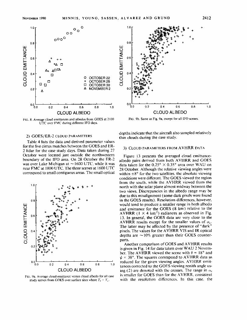
FIG. 8. Average cloud emittances and albedos from GOES at 2100UTC over FMC during different IFO days.
HJoz<v-v--
LM
O...Io
++%,_._1_, _r . +% +-_ _+ "r,. ++
0.8 *_,+_.***_.+ + . * +
+ +++ +
+ ..4- +
+ _±"-,L.+
0.4 +4" "t'4"._
+ +
0.0 , I * I , I , I *
0.0 0.2 0.4 0.6 0.8
CLOUD ALBEDO
FIG. 9b. Same as Fig. 9a, except for all IFO scenes.
I
1.0
2) GOES/ER-2 CLOUD PARAMETERS
Table 4 lists the data and derived parameter valuesfor the five cirrus matches between the GOES and ER-2 lidar for the case study days. Data taken during 27October were located just outside the northwesternboundary of the IFO area. On 28 October the ER-2was over Lake Michigan at _ 1600 UTC, while it wasnear FMC at 1800 UTC. The three scenes at 1600 UTCcorrespond to small contiguous areas. The small optical
itl¢DZ<V--
Illa
O._1¢D
1.0
0.8
0.6
0.4
0.2
+++ +.,.+
-,-"+ ÷-,-+ +.11.¢" + +
+ +
+ +++_._r.++'_¢_ +
.'it+++ +÷+_, ÷_+_ _"+ # _, +.4¢-
,.e¥
_1:+-_I: t-+I. 4._++ +
+
+, + +
+ +
+
0.0 i I I i I i I | I
0.0 0.2 0.4 0.6 0.8 1.0
CLOUD ALBEDO
FIG. 9a. Average cloud emittance versus cloud albedo for all casestudy scenes from GOES over surface sites where T, = Tc.
depths indicate that the aircraft also sampled relativelythin clouds during the case study.
3) CLOUD PARAMETERS FROM AVHRR DATA
Figure 13 presents the averaged cloud emittance-albedo pairs derived from both AVHRR and GOESdata taken for the 0.25 ° × 0.35 ° area over WAU on28 October. Although the relative viewing angles werewithin +8 ° for the two satellites, the absolute viewingconditions were different. The GOES viewed the regionfrom the south, while the AVHRR viewed from thenorth with the solar plane almost midway between thetwo views. Discrepancies in the albedo range may bedue to this misalignment (some dark pixels were foundin the GOES results). Resolution differences, however,would tend to produce a smaller range in both albedoand emittance for the GOES (8 km) relative to theAVHRR (1 × 4 km 2) radiances as observed in Fig.13. In general, the GOES data are very close to theAVHRR results except for the smaller values of ac.The latter may be affected by the presence of "dark"pixels. The values for the AVHRR VIS and IR opticaldepths are _ 10% greater than their GOES counter-parts.
Another comparison of GOES and AVHRR resultsis given in Fig. 14 for data taken over WAU 2 Novem-ber. The AVHRR viewed the scene with 0 = 18° and_b= 38 °. The squares correspond to AVHRR data asreduced for the given viewing angles. AVHRR emit-tances corrected to the GOES viewing zenith angle us-ing (2) are denoted with the crosses. The range in ,_is smaller for GOES than for the AVHRR, consistentwith the resolution differences. In this case, the

2413 MONTHLY WEATHER REVIEW
TABLE 3. Reflectance parameters computed for all GOES-surface lidar data.
VOLUME I 18
Time Cases 0 ¢ O(UTC) (IFO) (°) (°) (°)
Nominal (using ×c) Reanalyzed (using ×'c)
All data (IFO) Case study All data (IFO) Case study
1330 4 80.2 106.6 109 1.28
1400 3 75.6 112.6 117 2.21
1430 2 71.3 118.6 124 1.071500 3 67.9 125.7 131 1.72
1600 5 61.0 140.0 146 2.93
1630 2 57.8 147.7 153 2.59
1700 6 57.6 156.6 160 2.58
1800 6 57.3 174.1 173 2.43
1830 1 56.1 177.1 175 3.65
1900 7 59.9 169.0 168 1.62
1930 4 61.1 160.8 162 1.73
2000 8 65.0 153.6 154 2.07
2030 5 68.3 146.5 147 1.56
2100 6 72.8 140.3 140 1.072130 4 76.2 133.6 132 1.12
2200 5 81.2 128.1 125 0.80
Totals and
means 71 67.2 145.4 -- 1.69
1.17 0.15 0.83 0.28 1.61 0.28 1.61
1.42 0.17 1.12 3.22 2.32 0.21 1.53
1.79 0.32 1.72 1.35 2.22 0.38 2.082.02 1.72 2.02 1.87 2.15 1.87 2.15
2.50 1.82 2.11 2.64 2.25 1.64 1.91
1.85 -- -- 3.06 2.18 -- --
2.90 1.57 2.93 1.96 2.21 1.20 2.23
2.96 1.95 6.21 1.92 2.33 1.48 4.86
2.06 -- -- 3.88 2.19 -- --
3.12 0.69 3.43 1.82 2.12 0.49 2.36
2.74 0.75 2.76 1.34 1.97 0.57 1.91
2.68 1.69 2.87 2.27 2.26 1.35 2.30
2.55 1.87 2.37 1.33 2.23 1.59 2.05
2.07 1.02 2.19 t.17 2.24 1.12 2.38
1.29 0.55 1.25 0.81 2.23 0.94 2.08
2.360.84 0.28 0.70 1.04 2.30 0.80
2.13 1.04 2.17 1.80 2.19 1.11 2.16
AVHRR data produce a much lower minimum cloudalbedo. The application of (2) appears to have pro-duced very similar emittances for the two datasets, al-though there is a 20% difference in the average valuesof re. The mean VIS optical depths differ by a factorof 2.
All of the coincident AVHRR and GOES data are
summarized in Table 5. The AVHRR IR optical depths
are consistently greater than the corresponding GOESvalues by _0.1. This difference indicates the possibilityof a calibration offset in the thermal channels. Despitethis obvious bias, the good relative agreement in Fig.14 between the corrected AVHRR emittances and the
GOES emittances suggests that ( 3 ) is a reasonable ap-proximation to the IR absorption optical depth. AnyIR scattering effects that are ignored here are apparently
1.0
uJOz 0.8
LLI 0.6
...1
O
rr o.4w>a
O o.2_JO
0.021
s,ll
J
r-
, I I I , I , I I I
220 230 240 250 260
CLOUD TEMPERATURE (K)
FIG. 10. Variation of cloud vertical emittance with cloud-center
temperature for all IFO (circles) and case study (squares) data fromGOES over surface lidar sites. Vertical lines denote standard devia-
tions. Dashed line adapted from Platt et al. (1987).
6
09¢/)LLIZ 4Y
"1- 3 I-II-
°O 2
O1
0 I i I I , I
21 220 230 240 2_0
CLOUD TEMPERATURE (K)
FIG. 11. Variation of cloud thickness with cloud-center temperature
for all IFO (circles) and case study (squares) data from GOES oversurface lidar sites. Vertical lines denote standard deviations.

NOVEMBER1990 MINNIS, YOUNG, SASSEN, ALVAREZ AND GRUND 2414
0.6"7,
0.5
zW
O 0.4
u_LLLLI
O o3OzOI-- 0.2OzI-x 0.1LLI
t-r-
0.0210
i I
220
,,J
,11
/i
i I
|
/
I I I i i
230 240 250 260
CLOUD TEMPERATURE (K)
FIG. 12. Variation of in frared volu me extinction ( absorption ) coef-
ficient with cloud-center temperature for all IFO (circles) and case
study (squares) data from GOES over surface lidar sites. Vertical
lines denote standard deviations. Dashed curve adapted from Plan
et al. (1987).
insignificant compared to the other error sources. Dif-ferences between the GOES and AVHRR values of r,.vary from scene to scene. Even when the times andangles are very close and the data appear similar as inFig. 13, there are substantial differences in z,.. OverFMC during 28 October, there is good agreement be-tween the parameters however. The outstanding dif-ferences may be attributable to a number of factorsthat are discussed in section 3e.
tance tends to plateau at (b _ 0.86, while cloud-centeremittance appears to level at (b _ 0.98. The loweremittances lead to diminished values of rc relative to
those derived for Tc.The emittance ratio, r, = (b( Tt)/(b(To), was com-
puted for discrete intervals of To. Mean values andstandard deviations of these ratios are shown in Fig.16. The emittance ratio increases almost linearly withdecreasing cloud center temperature. Standard devia-
tions about a given mean rat,o are less than 0.1. Theemittance ratio is close to unity for Tc < 215 K.
The well-correlated variation of r, suggests the pos-sibility that Tt as well as Tc may be retrieved with VIS-IR radiance pairs. This ratio integrates many of theother parameters examined earlier. For example, cloudthickness in Fig. 1 ! is least at the highest altitudes andincreases before leveling or even decreasing for tem-peratures around 235 K. For the highest clouds, thereis little difference between T_ and Tt because the clouds
are not very thick. Since cloud depths are greater atlower altitudes, it is possible to sense radiation fromareas deep within the cloud thereby causing greaterdifferences between Tc and Tt. As the depth of the clouddecreases, the ratio should approach unity. At highertemperatures ( Tc > 250 K), the relationship of r, toT_ may not be as well defined because liquid waterbecomes more common and the mean cloud depthmay not be dependent on Tc. Whether the relationshipshown in Fig. 16 is typical for all observing angles isalso unknown. Additional sampling from other anglesand over a wider variety of temperatures would helpto better define the relationship between r, and Tc.However, the results shown in Figs. l l, 12, and 16suggest that it may be possible to obtain reasonableestimates of h and Tt over a limited range of To.
d. Results and discussion fi_r cloud-top temperatureswith GOES
The analyses discussed above were also performedfor the GOES-derived emittances for Tz = :Ft. A plotof all of the mean cloud emittance-albedo pairs isshown in Fig. 15. The largest concentrations of dataare found for _b(Tt) < 0.8. In general, ac is greater fora given value Of_b than it is in Fig. 9b. Cloud-top emit-
e. Emittance uncertainties
The parameter values derived here are subject toconsiderable uncertainty as evidenced by the results inTable 5 and the large standard deviations in earlierfigures. Potential sources of error abound in an analysisof this type due to the large number of variables andthe nonuniformity of cirrus clouds.
Parameters derived from the lidar essentially provide
TABLE 4. Observed and computed cloud properties for case study ER-2 data.
Dark
Time Lat. Lon. T, Tc h pixel
Day (UTC) (°N) (°W) (K) (K) (km) _-c r, _ (%) r_ _'
27 1830 45.8 93.1 290.0 225.0 0.5 0.12 0.69 5.73 0 0.46 3.86
1900 45.3 92.5 288.5 234.0 0.5 0.14 0.51 3.43 0 0.39 2.64
1930 44.9 91.1 288.4 234.0 0.5 0.24 0.73 2.91 3 0.61 1.68
28 1600 44.6 87.0 283.0 229.0 3.7 0.43 0.86 1.99 0 0.84 1.95
1600 44.5 87.1 283.0 229.0 3.7 0.42 0.92 2.12 0 0.91 2.10
1600 44.5 87.1 283.0 229.0 3.7 0.45 1.00 2.21 0 0.99 2.21
1800 43.6 89.4 288.9 228.0 1.5 0.28 0.90 3.23 0 0.69 2.57

2415 MONTHLY WEATHER REVIEW VOLUME II8
LU
Z
LU
a::DO_.1
(D
1.0
0.8
0.6
0.4
O
0.2 O+
++
÷
++O
+ + + +O+
_o_
+
0 +0o e
0 GOES 73.0 52.3 140.3
++ + AVHRR 73.1 48.9 146.3
, i , i , i i i , i
0"00.0 0.2 0,4 0.6 0.8 1.0
CLOUD ALBEDO
FIG. 13. Comparison of cloud albedos and emittances derived from28 October 1986 GOES and AVHRR data taken at _2100 UTCover WAU.
a two-dimensional view of the cirrus clouds. The va-
lidity of the assumption that zc, h, and zt represent the
average cloud heights within the large areas covered by
the strip of pixels is dii_cult to evaluate. One means
of estimating how well the lidar data represent the large-area cloud characteristics is to examine the differences
between the strip of pixels and surrounding areas. The
rms difference between the emittances for the strip and
the box containing the strip is 0.05 or 7%. This differ-
ence is equivalent to a +_0.7 km variation in cloud-
center height between the strip and the box. Changes
of 2 km in cloud-center altitude during a given half
hour are common as seen in Fig. 1. The variations in
the small-scale lidar data are greater than those in the
large-scale satellite data as expected.
Assuming that the large-scale differences are repre-sentative of the lidar-satellite scale differences, it is es-
timated that the use of lidar data to set zc causes an
uncertainty in _a of + 10% based on an average value
for (a of 0.62. Note that no clouds with (b < 0. l were
included in the analysis because of the cloud-detection
threshold of 3 K. A conservative estimate of the un-
certainty in Ts is _+2 K. Inclusion of this error raises
the overall uncertainty in (a to -+ 13%. This uncertainty
in ca is equivalent to a +-20% uncertainty in re for a
given scene over the range of optical depths considered
here. The AVHRR-GOES comparisons are, on aver-
age, within this uncertainty level. The average IR op-
tical thickness is 0.96 for all 71 scenes. From the strip
and box comparison, it is also estimated that zt and h
have uncertainties of +-0.7 km.
Another source of uncertainty in (a is the use of a
mean cloud height for the entire scene. This error
source may be examined by performing a pixel-by-pixel
analysis on a scene that varies systematically with time.
One example is the cloud over FMC between 2020 and
2050 UTC. The GOES pixels from the corresponding
wind strip data were averaged in lines perpendicular
to the wind vector. Using the wind speed, these aver-
aged pixels were converted to times and aligned with
the lidar-defined cloud parameters. The results shown
in Fig. 17 indicate good alignment between the two
datasets. In this case, it appears that the lidar data pro-
vide an accurate cross section of the cloud. The GOES
reflectance increases as the cloud thickens and T in-
creases as Zc lowers. Equations ( l ) and (5) were applied
to each average pixel using Tc derived from Fig. 17 to
determine re and zv. Figure 18 shows the variation of
the parameters with time. Although the thin part of
the cloud is detected with the IR data, a value for rv is
not computed since the reflectances are lower than that
for clear skies. Nevertheless, the mean values for 7e
and _b derived on a pixel-by-pixel basis are 0.59 and
0.54, respectively, compared to 0.62 and 0.59 derived
for the entire scene using a mean value of z_. This
comparison suggests that the error in _b for using the
mean cloud height is around 10% with a slight tendency
to bias the values to the high end because of nonlinear
effects. While these results may not represent all cases,
they indicate that the use of a mean cloud height for
the analysis is a reasonable approach.
4. Relationship between VIS and IR parameters
a. Scattering efficiency ratio
For a given cloud particle with cross-sectional area
2_ra 2, the VIS scattering cross section is
flv= Q_a27ra 2,
and the IR absorption cross section is
LLIO
z
uJa
o.._1
L)
1.0
0.8
0.6
0.4
0.2
0.00.0
+
[]
O++ ++
t_o",q []
++ _[]
o%
121I-I 0o 0
O GOES 67.1 52.3 154.5[] AVHRR 67.9 17.7 37.8+ CORRECTED AVHRR
i | t , i , l
0.2 0.4 0.6 0.8
CLOUD ALBEDO
FIG. 14. Same as Fig. 13, except for2 November 1986 at _2000 UTC.
i I
1.0
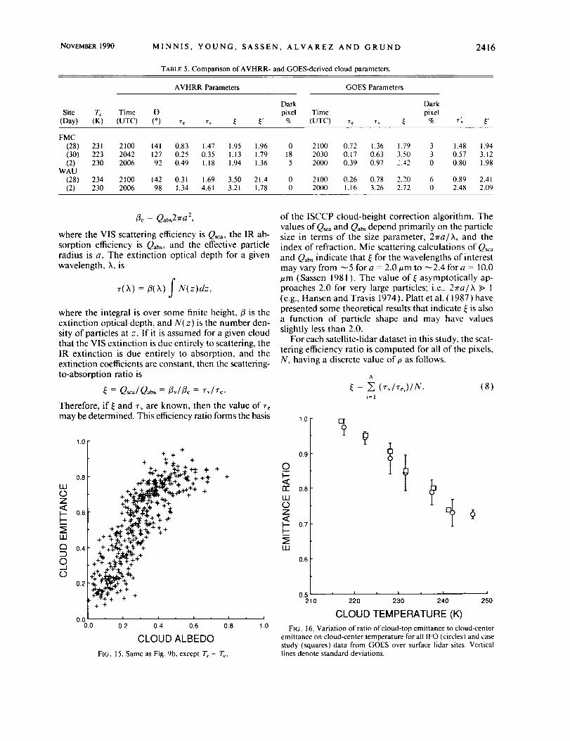
NOVEMBER 1990 MINNIS, YOUNG, SASSEN, ALVAREZ AND GRUND 2416
TABLE 5. Comparison of AVHRR- and GOES-derived cloud parameters.
AVHRR Parameters GOES Parameters
Dark Dark
Site T¢ Time O pixel Time pixel(Day) (K) (UTC) (°) r¢ rv _ _' % (UTC) r_ rv _ % r'v _'
FMC
(28) 231 2100 141 0.83 1.47 1.95 1.96 0 2100 0.72 1.36 1.79 3 1.48 1.94(30) 223 2042 127 0.25 0.35 1.13 1.79 18 2030 0.17 0.63 3.50 3 0.57 3.12(2) 230 2006 92 0.49 I. 18 1.94 1.36 5 2000 0.39 0.97 2.42 0 0.80 1.98
WAU
(28) 234 2100 142 0.31 1.69 3.50 21.4 0 2100 0.26 0.78 2.20 6 0.89 2.41(2) 230 2006 98 1.34 4.61 3.21 1.78 0 2000 1.16 3.26 2.72 0 2.48 2.09
13e = Qabs2ra 2,
where the VIS scattering efficiency is Q_ca, the IR ab-
sorption efficiency is Qabs, and the effective particle
radius is a. The extinction optical depth for a given
wavelength, X, is
r(X) = fl(X) f N(z)dz,
where the integral is over some finite height, 13 is the
extinction optical depth, and N(z) is the number den-
sity of particles at z. If it is assumed for a given cloud
that the VIS extinction is due entirely to scattering, the
IR extinction is due entirely to absorption, and the
extinction coefficients are constant, then the scattering-
to-absorption ratio is
= Osca/Qabs = _v/fle = rv/re.
Therefore, if _ and rv are known, then the value of re
may be determined. This efficiency ratio forms the basis
1.0
0.8
0.6
l 0.4
qO
0.2
0.0 , I
0.0 1.0
+
+ +
+ _. +
+._4ri"*'¢ + .+ +
+ "r_" -I_=tr_ql_. "-I-' "t-
++Nq+/:++ _ ._ +%-T-?,,_-++ ++-¢g+',t"+
++ .÷'+* +
WAI,_Im" _+ +
+ +
i | . I , l l l
0.2 0.4 0.6 0.8
CLOUD ALBEDO
FIG. 15. Same as Fig. 9b, except T, = T_.
of the ISCCP cloud-height correction algorithm. The
values of Q_ and Qa_ depend primarily on the particle
size in terms of the size parameter, 27ra/X, and the
index of refraction. Mie scattering calculations of Q_:,
and Q, bs indicate that _ for the wavelengths of interest
may vary from _ 5 for a = 2.0 um to _ 2.4 for a = I 0.0
tam (Sassen 1981 ). The value of _ asymptotically ap-
proaches 2.0 for very large particles; i.e., 27ra/X > 1
(e.g., Hansen and Travis 1974). Platt et al. (1987) have
presented some theoretical results that indicate _ is also
a function of particle shape and may have values
slightly less than 2.0.
For each satellite-lidar dataset in this study, the scat-
tering efficiency ratio is computed for all of the pixels,
N, having a discrete value of p as follows.
N
= _, (rWr_,)lN.i=l
(8)
O
<C£w0
w
1.0
0.9
0.8
0.7
0.6
0,5 i , i , i i
210 220 230 240 250
CLOUD TEMPERATURE (K)
FIG. 16. Variation of ratio ofcloud-top emittance to cloud-centeremittance on cloud-center temperature for all IFO (circles) and casestudy (squares) data from GOES over surface lidar sites. Verticallines denote standard deviations.

2417 MONTHLY WEATHER REVIEW VOLUME 118
3oI20v
_Z 10
0.0
_ul 0,0
90" '
°5t0.4
O- 0.3
0_2J
0.1 , i , i ,
280I_2_°r_
_ 26°r_ __" 250f240
230 ' ' • i ,
2020 2030 2040 2050UTC
FIG. 17.Comparisonof GOESand lidar observationsalong windvectorover FMC during 28October 1986.
Only one temperature, To, is used to compute re for agiven dataset since only one average cloud height isderived for each time. Changes in the actual cloudheight and thickness within the scene (e.g., Fig. 1 ) tendto introduce variations in re for a given reflectance•Thus, the mean value of _ is computed for each cloudreflectance value to minimize the effects of cloud height
variability.Visible optical depths for the case study GOES data
are given in Table 2. Tables 3-5 summarize the resultsof applying (8) to all of the data. Despite the differencesbetween the values ofrv for IFO and case study resultsin Table 3, two similarities are quite evident in a com-parison of the respective scattering efliciencies. For bothdatasets, the scattering efficiency appears to increasewith decreasing 00 and increasing O. At high values of8o, _ is well below the expected limit of 2. The averagevalues of _ are also very close, 2.17 and 2.13, for thecase study and IFO, respectively. In Table 4, the greatestvalues of _ also occur near local noon ( 1800 UTC).
b. Reanalyzed visible data
The temporal dependencies of rv and _j are not re-alistic. They are primarily due to shortcomings in theanalysis treatment ofxc. The anisotropy of the reflectedradiation field for real clouds depends on the opticalthickness, incident radiation, microphysical propertiesof the cloud, and the morphology of the cloud field.The value of Xc used here is fixed for a given set of
angles and represents an empirical average for all cloudtypes. The average cloud optical depth in the bidirec-
tional reflectance model used here is probably close to10, while rv for the clouds analyzed in this study isgenerally smaller than 2. Since cirrus clouds are theonly type considered here and the angles are fixed fora given hour, it is likely that Xc will be biased withrespect to local time. There will also be random errorsin X_ due to variations in microphysics, morphology,and cloud optical depth for a given hour. The mag-nitudes of these errors are currently unknown, but arepotentially large. Assuming that the time samplingrepresents a random sampling of ×_, the averages ofvarious parameters derived from all times should berelatively unbiased.
Using the assumption that the mean value of _ isindependent of time, new values of ×c were determinedfrom (5) using the observations of re and the meanscattering ratio of2.13. These new values were averagedat each time. The means, denoted as x_, are given inTable 6 with the mean nominal values from the bidi-rectional reflectance model. The results indicate more
anisotropy in the cirrus reflectance pattern than in theempirical model. The data of Takano and Liou (1989b)indicate that reflectance anisotropy diminishes withincreasing optical depth for scattering by hexagonalcolumns. Thus, the smaller optical depths of the cloudshere compared to those for the clouds in the empirical
model are probably responsible for the larger range ofX" compared to Xc.
To eliminate the temporal (angular) dependence ofrv, the data were reanalyzed using x'. The values ofthe visible optical depth and the scattering ratios de-termined from the reanalysis are listed in Tables 2-5and denoted with the primed variables, r" and _', re-spectively. Values of _' for the AVHRR data werecomputed by changing the nominal values ofx_ so thatthe derived value of z" for the AVHRR data was equal
to r" for the corresponding GOES data. In general, the
5O
40 f
30
2.0
10
00
15
10
05
O0
_0
f
J °8106
04
O2 j
0.0 , , , i ,
2020 2030 2040
UTC
FIG. 18. Cloud optical properties derived from Fig. 17.
205O
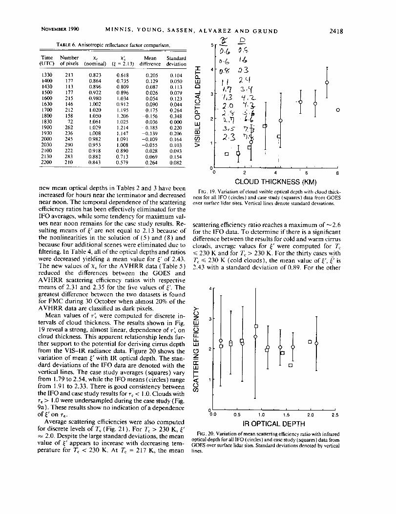
NOVEMBER 1990 M I N N ! S,
TABLE 6. Anisotropic reflectance factor comparison.
YOUNG, SASSEN, ALVAREZ AND GRUND
"1-
Time Number ×c X_ Mean Standard(UTC) of pixels (nominal) (4 = 2.13) difference deviation
f--1330 213 0.823 0.618 0.205 0.104 13.1400 177 0.864 0.735 0.129 0.050 ILl1430 113 0.896 0.809 0.087 0.113 ¢"11500 177 0.922 0.896 0.026 0.079 ....I1600 215 0.980 1.034 0.054 0.123 <i:
O1630 146 1.002 0.912 0.090 0.044 --
1700 212 1.020 1.195 -0.175 0.264 12.1800 158 1.050 1.206 -0.156 0.348 O1830 72 1.061 1.025 0.036 0.000 LM1900 262 1.029 1.214 -0.185 0.220 ....I1930 236 1.008 1.147 0.139 0.206 113
2000 245 0.982 1.091 -0.109 0.164 032030 290 0.953 1.008 -0.055 0.1032100 222 0.918 0.890 0.028 0.0932130 283 0.882 0.713 0.069 0.1542200 210 0.843 0.579 0.264 0.082
5
0,b 0,_
4 0._ 03
II 2.q
a /,....Z '4,2_
2.o "¢,2,-
.3,5 _'I
1
0 . . | ,I . ,•
2
0
reduced the differences between the GOES and
AVHRR scattering efficiency ratios with respective
means of 2.31 and 2.35 for the five values of _'. The 4 -
greatest difference between the two datasets is found
for FMC during 30 October when almost 20% of the
AVHRR data are classified as dark pixels. >-
Mean values of r" were computed for discrete in- OZ 3
tervals of cloud thickness. The results shown in Fig. u.I
19 reveal a strong, almost linear, dependence oft" on
cloud thickness. This apparent relationship lends fur- EL.ii
ther support to the potential for deriving cirrus depth ua
from the VIS-IR radiance data. Figure 20 shows the (5 z
variation of mean _' with IR optical depth. The stan- Zfl:
dard deviations of the IFO data are denoted with the t,u
vertical lines. The case study averages (squares) varyfrom 1.79 to 2.54, while the IFO means (circles) range < 1
from 1.91 to 2.33. There is good consistency between Oca0
the IFO and case study results for re < 1.0. Clouds with
7"e> 1.0 were undersampled during the case study (Fig.
9a). These results show no indication of a dependence 0of _' on re. 0.0
Average scattering efficiencies were also computed
for discrete levels of Tc (Fig. 21 ). For Tc > 230 K, _'
2.0. Despite the large standard deviations, the mean
value of _' appears to increase with decreasing tem-
perature for Tc < 230 K. At Tc = 217 K, the mean
i I t | t | i I i I
0.5 1.0 1.5 2.0 2.5
IR OPTICAL DEPTH
FIG. 20. Variation of mean scattering el_ciency ratio with infraredoptical depth for all IFO (circles) and case study (squares) data fromGOES over surface lidar sites. Standard deviations denoted by verticallines.
CLOUD THICKNESS (KM)new mean optical depths in Tables 2 and 3 have been
FIG. 19. Variation of cloud visible optical depth with cloud thick-increased for hours near the terminator and decreased hess for all IFO (circles) and case study (squares) data from GOESnear noon. The temporal dependence of the scattering over surface lidar sites. Vertical lines denote standard deviations.
efficiency ratios has been effectively eliminated for the
IFO averages, while some tendency for maximum val-
ues near noon remains for the case study results. Re- scattering efficiency ratio reaches a maximum of _2.6
suiting means of _' are not equal to 2.13 because of for the IFO data. To determine if there is a significant
the nonlinearities in the solution of (5) and (8) and difference between the results for cold and warm cirrus
because four additional scenes were eliminated due to clouds, average values for _' were computed for T_
filtering. In Table 4, all of the optical depths and ratios _< 230 K and for Tc > 230 K. For the thirty cases with
were decreased yielding a mean value for _' of 2.43. T_ _< 230 K (cold clouds), the mean value of _', _-_ is
The new values of Xc for the AVHRR data (Table 5) 2.43 with a standard deviation of 0.89. For the other
2418
J'' _ , I ! , I
q
4 6 8
2419 MONTHLY WEATHER REVIEW VOLUME I 18
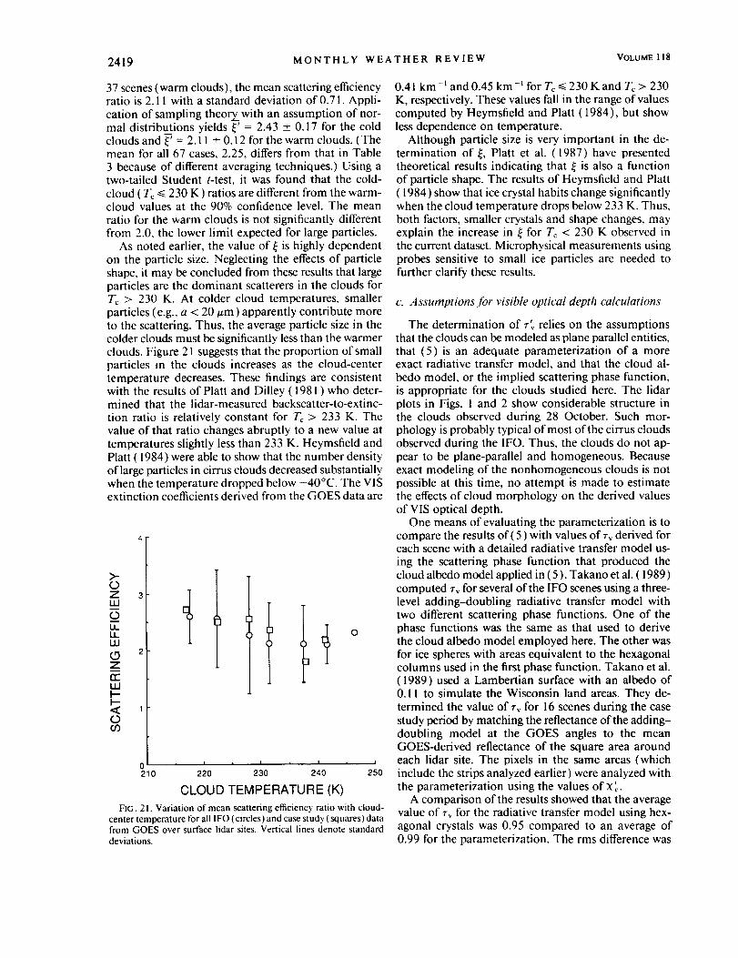
37 scenes (warm clouds), the mean scattering efficiencyratio is 2.11 with a standard deviation of 0.71. Appli-
cation of sampling theory with an assumption of nor-mal distributions yields _' = 2.43 ___0.17 for the coldclouds and _' = 2.11 + 0.12 for the warm clouds. (Themean for all 67 cases, 2.25, differs from that in Table3 because of different averaging techniques.) Using atwo-tailed Student t-test, it was found that the cold-
cloud ( Tc _<230 K) ratios are different from the warm-cloud values at the 90% confidence level. The mean
ratio for the warm clouds is not significantly differentfrom 2.0, the lower limit expected for large particles.
As noted earlier, the value of _ is highly dependenton the particle size. Neglecting the effects of particleshape, it may be concluded from these results that largeparticles are the dominant scatterers in the clouds forTc > 230 K. At colder cloud temperatures, smallerparticles (e.g., a < 20 _m) apparently contribute moreto the scattering. Thus, the average particle size in thecolder clouds must be significantly less than the warmerclouds. Figure 21 suggests that the proportion of smallparticles m the clouds increases as the cloud-centertemperature decreases. These findings are consistentwith the results of Platt and Dilley ( 1981 ) who deter-mined that the lidar-measured backscatter-to-extinc-
tion ratio is relatively constant for Tc > 233 K. Thevalue of that ratio changes abruptly to a new value attemperatures slightly less than 233 K. Heymsfield andPlatt (1984) were able to show that the number densityof large particles in cirrus clouds decreased substantiallywhen the temperature dropped below -40°C. The VISextinction coefficients derived from the GOES data are
>-0zLLI0LJ-
LJ-
LLI
ZI
n-"LLJ
<0CO
0
0 i i i i i210 220 230 240 250
CLOUD TEMPERATURE (K)
FIG. 21. Variation of mean scattering efficiency ratio with cloud-center temperature for all IFO (circles) and case study (squares) datafrom GOES over surface lidar sites. Vertical lines denote standarddeviations.
0.41 km -1 and 0.45 km-I for Tc _<230 K and T_ > 230
K, respectively. These values fall in the range of valuescomputed by Heymsfield and Platt (1984), but showless dependence on temperature.
Although particle size is very important in the de-termination of _, Platt et al. (1987) have presentedtheoretical results indicating that _ is also a functionof particle shape. The results of Heymsfield and Platt(1984) show that ice crystal habits change significantlywhen the cloud temperature drops below 233 K. Thus,both factors, smaller crystals and shape changes, mayexplain the increase in _ for Tc < 230 K observed inthe current dataset. Microphysical measurements usingprobes sensitive to small ice particles are needed tofurther clarify these results.
c. Assumptions Jor visible optical depth calculations
The determination of z" relies on the assumptionsthat the clouds can be modeled as plane parallel entities,
that (5) is an adequate parameterization of a moreexact radiative transfer model, and that the cloud al-bedo model, or the implied scattering phase function,is appropriate for the clouds studied here. The lidarplots in Figs. 1 and 2 show considerable structure inthe clouds observed during 28 October. Such mor-phology is probably typical of most of the cirrus cloudsobserved during the IFO. Thus, the clouds do not ap-pear to be plane-parallel and homogeneous. Becauseexact modeling of the nonhomogeneous clouds is notpossible at this time, no attempt is made to estimatethe effects of cloud morphology on the derived valuesof VIS optical depth.
One means of evaluating the parameterization is tocompare the results of( 5 ) with values ofrv derived foreach scene with a detailed radiative transfer model us-
ing the scattering phase function that produced thecloud albedo model applied in (5). Takano et al. ( 1989 )computed zv for several of the IFO scenes using a three-level adding-doubling radiative transfer model withtwo different scattering phase functions. One of thephase functions was the same as that used to derivethe cloud albedo model employed here. The other wasfor ice spheres with areas equivalent to the hexagonalcolumns used in the first phase function. Takano et al.(1989) used a Lambertian surface with an albedo of0.11 to simulate the Wisconsin land areas. They de-
termined the value of rv for 16 scenes during the casestudy period by matching the reflectance of the adding-doubling model at the GOES angles to the meanGOES-derived reflectance of the square area aroundeach lidar site. The pixels in the same areas (whichinclude the strips analyzed earlier) were analyzed withthe parameterization using the values of x'.
A comparison of the results showed that the averagevalue of z, for the radiative transfer model using hex-agonal crystals was 0.95 compared to an average of0.99 for the parameterization. The rms difference was

NOVEMBER1990 MINNIS, YOUNG, SASSEN, ALVAREZ AND GRUND 2420
17%. Although the 0.04 mean difference is not statis-tically significant, it is expected for several reasons. TheTakano et al. (1989) results include all of the pixels inthe region, while the results from (5) exclude all darkpixels. Furthermore, the radiative transfer model doesnot include ozone absorption. Exclusion of the darkpixels and inclusion of ozone absorption would bothtend to increase the mean model-derived optical depthby a few percent. The rms differences are most likelydue to the use of a Lambertian surface albedo in the
adding-doubling model and the use of a fixed value ofX_ for each hour in (5). The mean value of_j for themodel results was 2.55 compared to 2.56 for the pa-rameterization. From these comparisons it is evidentthat (5) is quite adequate for parameterizing the de-tailed radiative transfer model for the range of opticaldepths seen in the case study. In addition, the goodagreement between the average derived values of _' overland and water at the same hour (i.e., 1600 UTC) inTable 4 indicates that (5) is useful over a reasonablerange of surface albedos.
The cirrus clouds observed during the IFO containedmixtures of hexagonal columns, plates, and aggregatesof various sizes and shapes ( Kajikawa and Heymsfield1989). Even water droplets were found in some ofthe warmer cirrus clouds (Sassen et al. 1990). In thisstudy, the visible radiances have been treated as if theywere reflected from a cloud composed entirely of onesize of hexagonal columns. Although exact evaluationof the uncertainty in r_ due to the use of the singlephase function is not possible, some inferences may bedrawn from the results to make a qualitative assessment
of the hexagonal column, cloud-albedo model.One indication of the reasonability of the model used
here is that the mean value of _ is close to the limit of2.0 expected for large particles, especially for thewarmer clouds. An examination of the results of Tak-
ano et al. ( i 989) reveal that the mean value of rv de-rived with the equivalent ice-sphere model was 30%greater than that for the hexagonal column model. Theresulting mean value of _ for the ice spheres is 2.9.These results indicate that the ice-crystal model is moreappropriate than the spherical model for interpretingthe cirrus reflectance data.
The adding-doubling model of Takano and Liou(1989b) was used to calculate the cloud reflectancesfor the angles corresponding to GOES and AVHRRin Table 5 using the values of z" and the hexagonalcolumn phase function. The resulting reflectances atthe GOES angles were ratioed to the correspondingreflectances at the AVHRR angles. For the three casesin which the GOES and AVHRR angles differed sig-
nificantly (30 October and 2 November), the averageratio for the adding--doubling results was 1.6 comparedto 1.3, the mean ratio of the GOES and AVHRR valuesof Xc. About half of the difference in the mean ratiosmay be due to the uncertainties in the values of X_ foreach individual case. Thus, the actual difference in the
ratios may be as small as 0.15. This limited result sug-gests that the actual scattering by the cirrus clouds maybe less anisotropic than expected for the hexagonalcrystal model. Although discrepancies between the mi-crophysical characteristics of the actual and modeledclouds are likely to cause differences between the ob-served and modeled radiation fields, some of the ten-
dency for more diffuse reflectance from the cirrus maybe due to shadowing effects as discussed below. A morecomplete analysis using mucl more data is requiredto better define typical cirrus reflectance anisotropy andthe single scattering phase function that accounts forit. Given the current knowledge of cirrus cloud radia-tive properties, however, the cloud albedo model usedin (5) appears to be adequate for computing r'v.
d Dark pixels
It is possible that the "dark" pixels noted earlier maybe caused by the extreme reflectance anisotropy ex-pected for very thin clouds. For small values oft, andO _ 120 °, there should be very little reflection fromthe cloud in the direction of the satellite as comparedwith its albedo to upwelling diffuse radiation from thesurface. Thus, the pixel may appear darker than a clearscene for the same viewing and illumination conditions.
Examples of the variations of 0 as a function of accomputed with (5) are shown in Fig. 22a for WAU at1400 and 1800 UTC. The corresponding values of osare 0.13 and 0.16, respectively, with a_ = 0.11. Therelationship between cloud albedo and optical depthdepends on the solar zenith angle resulting in a diver-gence of the curves at larger values of ac. Additionalcalculations were performed for #0 = 0.4: ×c = 1; and
ps = 0.04, 0.08, 0.16, 0.32, and 0.64; with a_ = 0.92ps.
0.7 m
0.6--t._ /9s0Z .16
0.5--I.-(,.)I..iJ 13--J 0.4i.kidn,"
rl O.3
>n," 0.2I.IJ03rno o.1 -
0.o I I I I [ !0.0 0.1 0.2 0.3 0.4 0.5 0.6
CLOUD ALBEDO
FIG. 22a. Theoretical top-of-the-almosphere visible reflectance overWAU for 1400 UTC (m = 0.13) and for 1800 UTC (p_ = 0.16).

2421 MONTHLY WEATHER REVIEW VOLUME 118
0
laJm._1.<
w>cwla.I(/3cn0
0.7 -- P,,
0.6 __.........64.32
0.5 -- .16.08.04
0.4
0.3
0.2
0.1
o.ol I I I I I0.0 0.1 0.2 0.3 0.4 0.5
CLOUD ALBEDO
FIG. 22b. Theoretical top-of-the-atmosphere visible albedos for
various surface albedos.
I0.6
The results are shown in Fig. 22b. For relatively darksurfaces, the measured reflectance increases monoton-ically with ac. Over bright surfaces, the reflectance ac-tually decreases first, then increases at greater cloudalbedos. A dark surface contributes little to the upwardflux, while the opposite is true for bright surfaces. Theincreased reflectance of a cloud to diffuse radiation
tends to trap some of the reflected radiation from thesurface. For thin clouds over bright surfaces, this effectcan result in a reflectance that is lower than that ob-
served for the clear-sky case. Additional calculationsfor other solar zenith angles indicate that the insertionof the thin cirrus cloud above the bright surface de-creases the albedo at lower sun angles, making the dis-crimination of clear and cloudy skies more difficultover deserts and other bright scenes. It is possible thatthis effect may also be important at certain angles andvalues of ×c over dark surfaces.
Although such a mechanism may cause some pixel
darkening, it is probably not the primary cause. Cloudshading is more likely to be the predominant cause ofdark pixels. For example, at altitudes of 10 km, a 2km thick cloud can cast a shadow that has its leadingedge removed at least 8 km horizontally on the surfacefrom the position of the cloud's leading edge for 00>t 45 °. Thus, the cloud and the portion of the surfaceaffected by direct transmission through the cloud can
easily be offset by one or more GOES pixels. The pro-jected line of sight from the satellite through a cloudwill not line up with the cloud's shadow unless O
180 ° . In most instances, therefore, the direct trans-mission from the surface through the viewed cloud willcome from the shadow of a different cloud. The diffusereflectance will result from the combined effects of the
various clouds in the vicinity. For a homogeneous
cloud field, an optically thick viewed cloud, or O= 180 °, such effects are negligible. Figures 1, 2, and17 provide ample evidence that the clouds observedduring the case study are neither optically thick norhomogeneous. In an inhomogeneous cloud field, it ispossible to observe a surface darkened by the shadowof a thick cloud through a thin cloud that produceslittle scattering of its own in the direction of the satellite.Thus, to the viewer in space a pixel appears to be acloud by virtue of its cold temperature, but is darkerthan expected for a clear scene.
This effect may be examined quantitatively by con-sidering (5). Use of that model implicitly assumes ahomogeneous cloud field. To consider an inhomoge-neous cloud field, let rs replace rv in (6), where rs isthe VIS optical depth of the cloud casting a shadowonto the surface in the line of sight of the observedcloud that has optical depth rv. Since the diffuse ra-diation emerging from the bottom of the clouds andreflecting from the surface is coming from all of theclouds in the field, let ac in the third term of (5) bereplaced by the average albedo of the observed and theshading cloud. The results of solving this inhomoge-neous version of (5) for two different observed clouds
are displayed in Fig. 23. The circles represent rs = rv.Viewing angles were fixed at 0 -- 52 ° and Xc variedwith 00, which changed with time as in the lower halvesof Tables 3 and 6. Clear-sky reflectance is denotedwith the dashed horizontal line.
The greatest effects of cloud inhomogeneities are seenfor r_ -- 0.25. Both shading clouds cause dark pixelsfor 00 < 81 o. Some dark pixels occur for rs -- rv for 00< 60 °. Calculations using smaller u0's produced nodark pixels. The thickness of the shading cloud becomesmore important as _t0increases. The impact of shading
on the observed cloud having rv = 1 is less pronouncedwith little likelihood of dark pixels for the range of/_o
0.4
_. 0.2
rno
O
1-,- SHADING CLOUD
• "r, = 0.25
-0 m
I_'r, = 1.00
.................o........ ....... 0.252_
o.1 - "J 0 0 [] [_.'r, 1.0
<_ _.-r, = 4.0
o.o I I I I I0.1 0.2 0.3. 0.4 0.5 0.6
COSINE SOLAR ZENITH ANGLE
FIG. 23. Effect of cloud shading on observed reflectance. Optical
depth of observed cloud is r_. Solid symbols, r_ = 1. Open symbols,
r_ = 0.25. Dashed line is clear-sky reflectance.
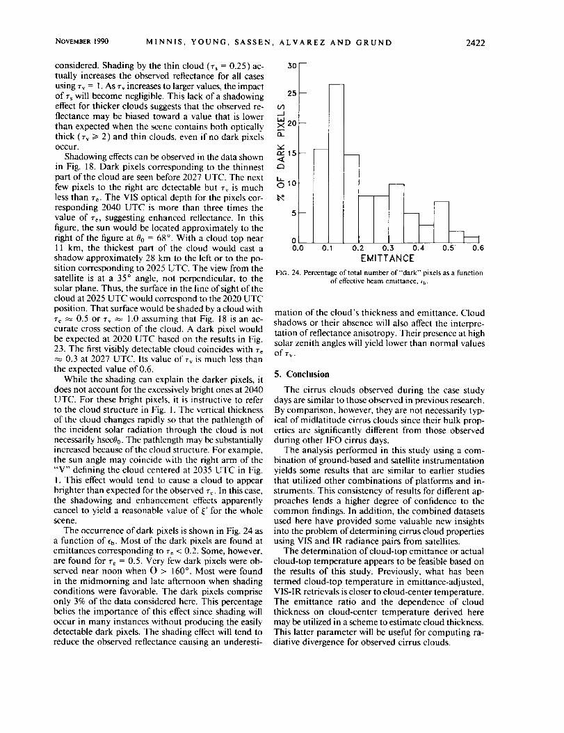
NOVEMBER1990 MINNIS, YOUNG, SASSEN, ALVAREZ AND GRUND 2422
considered. Shading by the thin cloud (r_ = 0.25) ac-tually increases the observed reflectance for all casesusing rv = 1. As rv increases to larger values, the impact
of rs will become negligible. This lack of a shadowingeffect for thicker clouds suggests that the observed re-flectance may be biased toward a value that is lowerthan expected when the scene contains both opticallythick (rv >/2) and thin clouds, even if no dark pixelsOccur.
Shadowing effects can be observed in the data shownin Fig. 18. Dark pixels corresponding to the thinnestpart of the cloud are seen before 2027 UTC. The next
few pixels to the fight are detectable but rv is muchless than re. The VIS optical depth for the pixels cor-responding 2040 UTC is more than three times thevalue of re, suggesting enhanced reflectance. In thisfigure, the sun would be located approximately to theright of the figure at 00 = 68 °. With a cloud top near11 km, the thickest part of the cloud would cast ashadow approximately 28 km to the left or to the po-sition corresponding to 2025 UTC. The view from thesatellite is at a 35 ° angle, not perpendicular, to thesolar plane. Thus, the surface in the line of sight of thecloud at 2025 UTC would correspond to the 2020 UTCposition. That surface would be shaded by a cloud withre _ 0.5 or rv _ 1.0 assuming that Fig. 18 is an ac-curate cross section of the cloud. A dark pixei wouldbe expected at 2020 UTC based on the results in Fig.23. The first visibly detectable cloud coincides with re
0.3 at 2027 UTC. Its value of rv is much less thanthe expected value of 0.6.
While the shading can explain the darker pixeis, itdoes not account for the excessively bright ones at 2040UTC. For these bright pixels, it is instructive to referto the cloud structure in Fig. 1. The vertical thicknessof the cloud changes rapidly so that the pathlength ofthe incident solar radiation through the cloud is notnecessarily hsec00. The pathlength may be substantiallyincreased because of the cloud structure. For example,the sun angle may coincide with the right arm of the"V" defining the cloud centered at 2035 UTC in Fig.1. This effect would tend to cause a cloud to appearbrighter than expected for the observed re. In this case,the shadowing and enhancement effects apparentlycancel to yield a reasonable value of _' for the wholescene.
The occurrence of dark pixels is shown in Fig. 24 asa function of _b. Most of the dark pixels are found atemittances corresponding to re < 0.2. Some, however,are found for re = 0.5. Very few dark pixels were ob-served near noon when O > 160 °. Most were found
in the midmorning and late afternoon when shadingconditions were favorable. The dark pixels comprise
only 3% of the data considered here. This percentagebelies the importance of this effect since shading willoccur in many instances without producing the easilydetectable dark pixels. The shading effect will tend toreduce the observed reflectance causing an underesti-
xilL-
rY<r'n
Lt.0
30--
25--
20--
15--
10--
5--
00.0 0.1 0.2 0.3 0.4 0.5" 0.6
EMITTANCE
FIG. 24. Percentage of total number of "dark" pixels as a functionof effective beam emittance, _b.
marion of the cloud's thickness and emittance. Cloud
shadows or their absence will also affect the interpre-tation of reflectance anisotropy. Their presence at highsolar zenith angles will yield lower than normal valuesof rv.
5. Conclusion
The cirrus clouds observed during the case studydays are similar to those observed in previous research.By comparison, however, they are not necessarily typ-ical of midlatitude cirrus clouds since their bulk prop-erties are significantly different from those observedduring other IFO cirrus days.
The analysis performed in this study using a com-bination of ground-based and satellite instrumentationyields some results that are similar to earlier studies
that utilized other combinations of platforms and in-struments. This consistency of results for different ap-proaches lends a higher degree of confidence to thecommon findings. In addition, the combined datasets
used here have provided some valuable new insightsinto the problem of determining cirrus cloud propertiesusing VIS and IR radiance pairs from satellites.
The determination of cloud-top emittance or actualcloud-top temperature appears to be feasible based onthe results of this study. Previously, what has beentermed cloud-top temperature in emittance-adjusted,VIS-IR retrievals is closer to cloud-center temperature.The emittance ratio and the dependence of cloudthickness on cloud-center temperature derived heremay be utilized in a scheme to estimate cloud thickness.
This latter parameter will be useful for computing ra-diative divergence for observed cirrus clouds.

2423 MONTHLY WEATHER REVIEW VOLUME118
The results indicate that scattering efficiencies aregreater for colder clouds. This finding holds promisefor improvements in determining the IR optical depthfrom reflected VIS data. Additional study, however, is
required to confirm this conclusion.From the examination of the reflectance data and
scattering efliciencies it is concluded that much workremains to adequately describe the scattered radiationfield for real cirrus clouds. Both theoretical and em-
pirical bidirectional reflectance models should be de-veloped for clouds composed of realistic particle shapes.As in the ISCCP model, the patterns should be devel-oped for various optical depths. Those models will re-quire confirmation with the aid of further observationaldata. The effects of cloud particle scattering in IR ra-diative transfer should also be examined observation-
ally.Cloud shadows are a problem for the interpretation
of cloud reflectances, especially for cirrus. The effectsare not limited to large solar zenith angles. Relativelyhigh viewing zenith angles can produce situations thatresult in the viewing of shadows, even for the near-zenith sun. It is apparent that analysis of a single pixelis most sensitive to shadowing problems. Some of theeffects may be diminished through averaging over sev-eral pixels. Other approaches to deal with shading needto be developed. Validations of cirrus scattering cal-culations must also consider these effects. The problemof shadows is not as important over water because of
the low surface albedo. Other problems in remotesensing of clouds such as partially cloud-filled pixelshave not been considered here. Future research effortsshould address these other factors.
Acknowledgments. The contributions of Messrs. P.Heck, R. Wheeler, and G. Gibson of Lockheed Engi-neering and Sciences Company to the satellite data re-duction and graphics are deeply appreciated. We alsothank Ms. S. Morgan of Computer Sciences Corpo-ration for her assistance in reducing the GOES data.Discussions with Dr. B. A. Wielicki of NASA LangleyResearch Center were also quite helpful. We wouldalso like to thank Drs. K. N. Liou and Y. Takano of
the University of Utah for making their radiativetransfer model available. The Madison lidar measure-
ments were supported by ARO Grant DAAG29-84-K-0069, ONR Grant N00014-87-K-0436, and NASAGrant NAAG i-882.
APPENDIX A
Low and thick cloud filtering
The presence of low clouds contaminates the datasince the analysis is predicated on the presence of onlyone cloud layer (the cirrus layer may contain two ormore distinct sublayers). The cloud heights are definedfor the upper-level cloud (generally, zb > 4 km) de-tected by the lidar. In some instances, the occurrence
of low clouds was either noted by the lidar operatorsor evident in the backscatter intensity plots. In othercases, the visual observations were not recorded or thelow clouds were located within the satellite-defined area
around the site, but beyond the observer's horizon.The datasets containing low clouds must either beeliminated or the pixels contaminated by low cloudsmust be removed. Elimination of all datasets contain-
ing low clouds would substantially reduce the numberof samples.
In order to define a simple preprocessing filter, it isfirst assumed that ac oc rv for small optical depths. Itis also assumed that, to a first approximation, p = TaO_ c
+ ps( 1 - c_c)2 and ac = pc. Using the definition of_j
(§ 3e) and (4), it can be shown that
_b = 1 -- exp(-kac/_t), (7)
where k is the constant of proportionality. Values fork are determined in the following manner. For a givensite and time, _b is computed with ( 1 ) for each cloudypixel having D > Ds and T < Ts - 3 K. The meanemittance is then computed for each value of D cor-responding to the approximated value of ac. Equation(7) is solved for k using each aibedo-emittance pair.
An average value of k is then computed for a specifiedsubset of the data. This procedure is applied using Tz= Tc.
To filter the data, it is assumed that low clouds are
generally brighter than cirrus, but their emittances de-pend on albedo, as in (7), in the same manner as cirrus.Thus, ifa maximum cloud albedo is known for a givencirrus emittance, then it may be assumed that any pixelsbrighter than that maximum contain some low clouds.The values of those maximum albedos, a .... must beestimated here. To determine those maximum values,
the histograms were first filtered manually to obtain aset containing no low clouds. The maximum albedofor each temperature (emittance) was extracted for ev-ery histogram at a given time. Data taken on 22 Oc-tober 1986, were used in the analysis. All maxima fora given time were compared to determine the greatestvalues for that time. Very little dependence on timewas found in this comparison. Therefore, the maximafrom all hours were combined. The resultant values
were then used to solve (7) for k using a least-squaresregression fit. The results were averaged to obtain thecoefficient, k .... which is used to define the maximumcloud albedo for a given emittance. The results of thisprocess yield kmax = 2.4. Thus, for a given time, (7)may be solved for amax using kmax and the emittance.Any pixel with ac > Ogmaxd- 0.025 is assumed to containlow clouds and is eliminated from further processing.The 0.025 increment is an estimate of the uncertaintyin amax resulting from the use of an approximation.
An example of this filtering is shown in Fig. A1 forthe data over FMC at 1930 UTC 28 October when low
clouds were noted in the observer's log. Crosses rep-resent individual pixels. The solid line represents Otma x

NOVEMBER 1990 MINNIS, YOUNG, SASSEN, ALVAREZ AND GRUND 2424
LUOz<
ILl
o
O....IO
1.0
0.8
++
÷**0.6 "+ +
'_.+
,÷0.4
0.2
+
++
$
_++
+
+ ++
+
++ + +
+ + +
0.0 ' , I , I i i . I
0.0 0.2 0.4 0.6 0.8 1.0
CLOUD REFLECTANCE
FIG. A I. Example of low-cloud filter application over FMC at
1930 UTC 28 October 1986. All data to right of solid line correspondto low clouds.
seen in Figs. 1 and 2, real cirrus clouds are anythingbut uniform and constant in altitude and depth. Anactual cloud field may also contain broken clouds withvariable optical depths. The nonuniformity of such realclouds blurs the distinction between the linear rela-
tionship for partly cloudy pixels and the exponentialdependency for variable thickness overcast pixels. Overland the ISCCP algorithm uses a threshold of 6 K colderthan the clear-sky temperature to determine cloudypixels (Rossow et al. 1988). Because of the low spatialvariability in T_ over the land areas in this study, it isassumed here that pixels colder than 7",- 3 K are over-cast. The data are not used, however, if there is evidence
of any significant breaks in the ceiling from the lidardisplays or if the mean IR optical depth is less than0.1. Very few breaks were seen over the sites on 28October. The cirrus observed on 27 October were
mostly scattered leading to the selection of only twoscenes for that day.
a
B
D, Dsh
k, kmax
computed using kma x. The vertical line, o/max = 0.20,is used at low reflectances because of larger uncertain-ties at those reflectance levels. This value is based on
a visual inspection of the data that contained lowclouds. The filtering process eliminates the pixels that Qa_, Q_aclearly contain low clouds (i.e., those to the right of r,the line). Some pixels containing both low and high T, Tsclouds, however, may remain in the data.
All cases having rv > 5.0 were also removed from To, Ttthe dataset. This arbitrary limit was imposed to min-imize the uncertainties in re, rv, and subsequent values Taof _j. The absolute error in derived optical depth in-
creases with increasing emittance. The value of Tc is Tz, T8also more uncertain for thick clouds than thinner
clouds. Thus, errors in emittance are greater for these tthick clouds. Their removal does not significantly affect uthe trends in the results. Inclusion of the thick clouds, Zb, Zc, Zthowever, greatly increases the noise in the data. Nocase study scenes were affected by the thick-cloudelimination.
O/c, o/d
o/s_ o/sd
O/max
APPENDIX B
Partially cloud-filled pixels /5' _/_'/_e
The use of (7) or (8) implicitly assumes that the 3'pixel is completely filled with cloud. While it is likely _a, _bthat some of the pixels are partially clear, definitive Omeans for determining which are overcast and which 0, 0oare partly cloudy are unavailable. Platt ( 1 .... . vposeda bispectral method to discriminate partly cloudy pixels ta, _0from those containing thin clouds. His technique re- _j
quires uniform blocks of constant height and thickness p, p_, pcfor detection of partly cloudy pixels. Detection of thinclouds allows variable thicknesses, but not heights. As aa
APPENDIX C
List of symbols
particle radiusPlanck function at 11.5 umobserved and clear-sky visible countscloud thickness
albedo coefficient, albedo coefficient formaximum cloud albedo
absorption and scattering efficienciescloud-top and -center emittance ratioobserved and clear-sky 11.5 um equivalent
blackbody temperaturescloud-center and -top 11.5 um equivalent
blackbody temperaturesclear-sky temperature estimated from sur-
face data
air temperatures at altitude z and at thesurface
timeozone abundancecloud-base, cloud-center, and cloud-top
altitudescloud and diffuse cloud albedos
clear-sky albedo, clear-sky diffuse albedomaximum albedo for high clouds at a
given emittanceextinction, scattering, and absorption cross
sections
density of particles in the mediumvertical emittance, beam emittance
single-scattering angleviewing zenith angle, solar zenith anglelatitude or wavelengthCOS0, COS00
scattering efficiency ratioobserved, clear-sky, and cloud visible re-
flectancevolume extinction coefficient

2425 MONTHLY WEATHER REVIEW VOLUME II8
re, rv infrared absorption and visible scatteringoptical depths
r5 visible scattering optical depth of shadingcloud
Ta, Tc, Tu ozone, downward cloud, and upwardcloud transmittances
longitude×5, ×c clear-sky and cloud anisotropic reflectance
factors
_b relative azimuth angleIFO Intensive Field Observations ( 19 October-
2 November 1986)IR infrared window (11.5 #m)
FMC Ft. McCoy, WisconsinUTC Coordinated Universal Time
MAD Madison, Wisconsin
WAU Wausau, WisconsinVIS visible (0.65 urn)
REFERENCES
Grund, C. J., and E. W. Eloranta, 1990: The 27-28 October 1986
FIRE IFO cirrus case study: optical properties of cirrus clouds
measured by the high spectral resolution lidar. Mort. 14"ea. Rev.,
118, 2344-2355.
Hahn, C. J., S. G. Warren and J. London, 1988: Surface synoptic
cloud reports for Wisconsin, 86 Oct-Nov 3. Cooperative Inst.
for Research in Environ. Sci., Campus Box 449, Univ. of Col-
orado, Boulder, CO, 15 pp.
Hansen, J. E., and L. D. Travis, 1974: Light scattering in planetary
atmospheres. Space Sci. Rev., 16, 527-610.
Heymsfield, A. J., and C. M. R. Platt, 1984: A parameterization ofthe particle size spectrum of ice clouds in terms of the ambient
temperature and the ice water content. J. Atmos. Sci., 41, 846-855.
Kajikawa, M., and A. J. Heymsfield, 1989: Aggregation of ice c_stals
in cirrus. J. Atmos. Sci., 46, 3108-3121.
Liou, K. N., 1973: Transfer of solar irradiance through cirrus cloud
layers. J. Geopkys. Res., 78, 1409-1418.
, 1986: Influence of cirrus clouds on weather and climate pro-
cesses: a global perspective. Mort. Wea. Rev., 114, 1167-1199.
, and G. D. Wittman, 1979: Parameterization of the radiative
properties of clouds. J. Atmos. Sci.. 36, 1261-1273.
McClatchey, R. A., R. W. Fenn, J. E. A. Selby, F. E. Volz and J. S.
Gating, 1973: Optical properties of the atmosphere (3rd edition ).AFCGRL-72-0497, 113 pp. [ NTIS-N73-18412.]
Minnis, P., and E. F. Harrison, 1984a: Diurnal variability ofregional
cloud and clear-sky radiative parameters derived from GOES
data, Part I: analysis method. J. Climate Appl. Meteor., 23, 993-1011.
, and --, 1984b: Diurnal variability of regional cloud and
clear-sky radiative parameters derived from GOES data, Part
!11: November 1978 radiative parameters. Z Climate Appl. Me-
teor., 23, 1032-1051.
, E. F. Harrison and G. G. Gibson, 1987: Cloud cover over the
eastern equatorial Pacific derived from July 1983 ISCCP data
using a hybrid bispectral threshold method..L Geophys. Res.,92, 4051-4073.
, P. W. Hock and E. F. Harrison, 1990: The 27-28 October
1986 FIRE Cirrus IFO case study: cloud parameter fields derivedfrom satellite data. Mort. Wea. Rev..ll8, 2426-2446.
Paltridge, G. W., and C. M. R. Platt, 1981: Aircraft measurements
of solar and infrared radiation and the microphysics of cirrus
cloud. Quart. Z Roy. Meteor Soe., 107, 367-380.
Plait, C. M. R., 1973: Lidar and radiometric observations of cirrus
clouds. J. Atmos. Sci.. 30, 1191-1204.
--, 1979: Remote sounding of high clouds, I: calculations of visible
and infrared optical properties from lidar and radiometer mea-
surements. J. Appl. Meteor., 18, 1130-1143.
--, 1983: On the bispectral method for cloud parameter deter-mination from satellite VISSR data: separating broken cloud
and semitransparent cloud. J. Climate AppL Meteor.. 22, 429-
439.
, and A. C. Dilley, 1979: Remote sounding of high clouds: II.Emissivity of cirrostratus. J. Appl. Meteor., 18, 1144-1150.
, and G. L. Stephens, 1980: The interpretation of remotely sensedhigh cloud emittances. J. Atmos. Sci., 37, 2314-2322.
, and A. C. Dilley, 1981: Remote sounding of high clouds: IV.
Observed temperature variations in cirrus optical properties. J.
Atmos. Sci., 38, 1069-1082.
, and --, 1984: Determination of cirrus particle single-scat-
tering phase function from lidar and solar radiometric data. AppL
Opt., 23, 380-386.
, D. W. Reynolds and N. L. Abshire, 1980: Satellite and lidar
observations of the albedo, emittance, and optical depth of cirrus
compared to model calculations. Mon. Wea. Rev., 108, 195-204.
, J. C. Scott and A. C. Dilley, 1987: Remote sounding of high
clouds, VI. Optical properties of midlatitude and tropical cirrus.J. Atmos. Sci., 44, 729-747.
Reynolds, D. W., and T. H. Vonder Haar, 1977: A bispectral methodfor cloud parameter determination. Mon. Wea. Rev.. 105, 446-457.
Rossow, W. B., L. C. Garder, P. Lu and A. Walker, 1988: International
Satellite Cloud Climatology Project (ISCCP), Documentationof cloud data. WCRP Report WMO/TD-No. 266, 122 pp.
[Available from Dr. W. B. Rossow at NASA Goddard SpaceFlight Center, Institute for Space Studies, 2880 Broadway, New
York, NY, 10025.]Sassen, K., 1981: Infrared (10.6 gm) scattering and extinction in
laboratory water and ice clouds. Appl. Opt., 20, 185-193.
--, C. J. Grund, J. Spinhirne, M. Hardesty and J. M. Alvarez,
1990: The 27-28 October 1986 FIRE 1FO cirrus case study: afive lidar view of cirrus cloud structure and evaluation. Mort.
Wea. Rev., 118, 2288-2312.
Shenk, W. E., and R. J. Curran, 1973: A multispectral method for
estimating cirrus cloud top heights. J. AppL Meteor.. 12, 1213-1216.
Schiffer, R. A., and W. B. Rossow, 1983: The International Satellite
Cloud Climatology Project ( ISCCP): the first project of the World
Climate Research Progamme. Bull. Amer Meteor Soc.. 64, 779-
784.
Spinhirne, J. D., D. I.. Hlavka and W. D. Hart, 1988:ER-2 lidarobservations from the October 1986 FIRE cirrus experiment.
NASA TM 100704, 49 pp. [NTIS-N89-21444.]
Starr, D. O'C., 1987: A cirrus-cloud experiment: intensive field ob-
servations planned for FIRE. Bull. Amer Meteor Soc., 68, 119-124.
Stephens, G. L., 1980: Radiative properties of cirrus clouds in the
infrared region. J. Atmos. Sci., 37, 435--446.Stuhlmann, R., P. Minnis and G. L. Smith, 1985: Cloud bidirectional
reflectance functions: a comparison of experimental and theo-retical results. Appl. Opt., 24, 396-401.
Suttles, J. T., R. N. Green, P. Minnis, G. U Smith, W. F. Staylor,
B. A. Wielicki, I. J. Walker, D. F. Young, V. R. Taylor and
L. L. Stowe, 1988: Angular radiation models for earth-atmo-sphere system: Volume l-Shortwave radiation. NASA RP 1184,
144 pp. [NTIS-N88-27677.]
Takano, Y., and K. N. Liou, 1989a: Radiative transfer in cirrus clouds:
I. Single scattering and optical properties of oriented hexagonal
ice crystals J. Atmos. Sci., 46, 3-20.
--, and --, 1989b: Radiative transfer in circus clouds: il. Theory
and computation of multiple scattering in an anisotropic me-dium. J. Atmos. Sci., 46, 21-38.
--, K. N. Liou and P. Minnis, 1989: Cirrus optical depth retrieval
from satellite-measured bidirectional reflectance. AMS Syrup.
on Role of Clouds in Atmos. Chem. and Global Climate, An-aheim, CA, Amer. Meteor. Soc., 178-180.