The 2016 HMT-WPC Winter Weather Experiment

25 January – 19 February, 2016

Weather Prediction Center College Park, MD

Final Report

April 8, 2016

1

1. INTRODUCTION The Hydrometeorology Testbed at the Weather Prediction Center (HMT-WPC) hosted 31 forecasters, researchers, and model developers (Appendix A) at its sixth annual Winter Weather Experiment (WWE) that took place from January 25 – February 19, 2016. Note that due to severe winter weather that impacted the Washington, D.C. area, two days of the experiment (January 25-26) were canceled. This year’s experiment allowed participants to explore innovative deterministic and ensemble-based snowfall forecasting techniques in the short range time period (Days 1-3). More specifically, the focus was on exploring the utility of both convection-allowing and non-convection-allowing models as well as downscaled snowfall forecasting techniques in the Day 1-2 period. For the first time, the experiment also explored the 6-12 hour time period for the purpose of identifying regional and temporal peaks in snowfall rates. The 2016 WWE continued the successful daily forecast briefing webinar that was introduced in last year’s WWE that again opened up a portion of the experiment to the general meteorological community allowing for remote participation. The science and operations goals of the 2016 WWE were to:

• Explore the Experimental High Resolution Rapid Refresh model (HRRRX) and the HRRR Time Lagged Ensemble (HRRR-TLE) provided by the NOAA Earth Systems Research Lab (ESRL) for winter weather forecasting.

• Explore the utility of an experimental version of the 3 km North American Mesoscale Forecast System Nest (NAMX) for winter weather forecasting.

• Explore the utility of the prediction of convective mesoscale snow banding by using increased spatial and temporal resolution of convection-allowing models (CAMs).

• Examine the utility of the WPC Watch Collaborator tool. • Create a probabilistic winter hazards impacts-based product. • Enhance collaboration among NCEP centers, WFOs, and NOAA research labs on winter weather

forecast challenges.

This report summarizes the activities, findings, and operational impacts of the 2016 WWE. 2. EXPERIMENT DESCRIPTION Daily Activities The 2016 experiment featured three forecasting activities. A detailed version of the daily schedule can be found in Appendix B.

a. Experimental Deterministic Snowfall Forecast

For the first forecasting activity of the day, participants were asked to use a combination of operational and experimental model guidance to issue a Day 1, 24-hour deterministic snowfall forecast valid 1200-1200 UTC for a storm/area of interest over the contiguous United States (CONUS). Participants were asked to draw contours of 1, 2, 4, 8, 12, and 20 inch snowfall amounts across the forecast domain. An example of a deterministic snowfall forecast produced during the

2

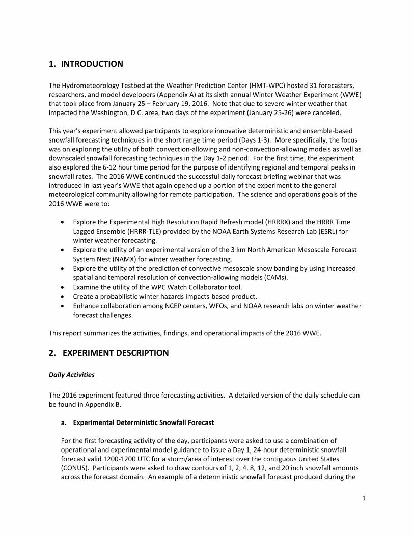
experiment is shown in Figure 1. Model implicit snowfall accumulation from the HRRRX, 6 and 24 hour change in snow depth from the HRRRX and NAMX, as well as derived snowfall from the High Resolution Adjusted Mean (HRAM) 3e and HRAM 3g ensembles were available for this activity.

Figure 1. 24-hour deterministic snowfall forecast valid from 12 UTC February 1, 2016 to 12 UTC February 2, 2016. Note the lowest contour value in this forecast was 4 inches.

b. Experimental Snowfall Rate Forecast

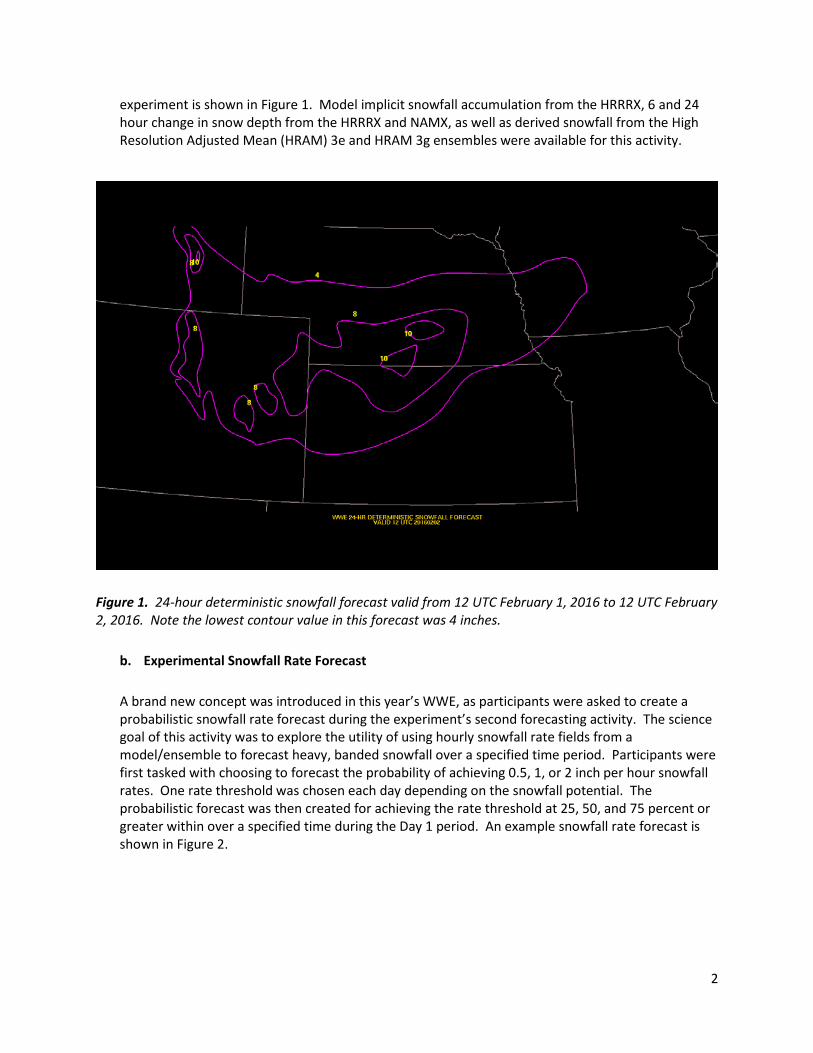
A brand new concept was introduced in this year’s WWE, as participants were asked to create a probabilistic snowfall rate forecast during the experiment’s second forecasting activity. The science goal of this activity was to explore the utility of using hourly snowfall rate fields from a model/ensemble to forecast heavy, banded snowfall over a specified time period. Participants were first tasked with choosing to forecast the probability of achieving 0.5, 1, or 2 inch per hour snowfall rates. One rate threshold was chosen each day depending on the snowfall potential. The probabilistic forecast was then created for achieving the rate threshold at 25, 50, and 75 percent or greater within over a specified time during the Day 1 period. An example snowfall rate forecast is shown in Figure 2.

3

Figure 2. Probability of a half inch of snow per hour occurring between 1800-2300Z on February 8, 2016. 25% or greater is represented by the yellow contour, 50% by the orange contour, and 75% by the red contour. c. Day 2 or 3 Winter Weather Hazards Product

The third forecast activity took place in the afternoon during which participants were asked to create a probabilistic Day 2 or Day 3 winter weather hazards impact-based product. As a starting point, threshold exceedance probabilities from the WPC Watch Collaborator tool for the watch/warning criteria for snow and freezing rain were used. From there, the participants utilized a variety of experimental and operational probabilistic guidance and then depicted areas of anticipated winter weather hazards in plain language. A rough guideline as to how the product developed is as follows: • Began with Watch Collaborator 30% likelihood of meeting/exceeding watch criteria for both

snow and freezing rain based on 24-hour WFO thresholds • Used probabilistic guidance and deterministic guidance to assess the predictability of the

impacting winter hazards • Used watch criteria CWA color-coded map as guidance to assess regional impact variability • Supplemented the winter weather hazards identified by the watch/warning criteria thresholds

with these potential hazards:

4

o heavy snow which may exceed watch/warning criteria in less than 6 hours o significant icing (greater than 0.05”) o ice glaze that may impact roadways (trace to 0.1”) during commute times o high winds (winds may reach or exceed threshold for blizzard conditions, typically

sustained 35 mph or higher over several hours) o rapidly falling temperatures o precipitation transition zones

One of the goals for this exercise was to enhance the predictability component of winter hazards forecasting in addition to highlighting impact criteria. Participants were given a free hand to experiment with various color schemes, descriptive plain language text, as well as the option to include or exclude numerical probabilities in their graphical depiction of winter hazards. An example of one of these forecasts is shown in Figure 3. A second goal of the exercise was to compile successful techniques and methods learned in this exercise, and determine whether they can be applied to plain language forecast products such as WPC’s National Forecast Chart.

Figure 3. Day 3 Winter weather hazards product valid from 1200 UTC February 7, 2016 to 1200 UTC February 8, 2016. The hazards being forecast are represented in the white text labels and the different colors represented the participants’ confidence in the hazards occurring. In this example, cyan represents low confidence, yellow medium confidence, and red high confidence. d. Forecast Discussion This year’s Winter Weather Experiment included a daily forecast discussion that was opened to the wider meteorological community (e.g. operational forecasters from local Weather Forecast Offices (WFOS), researchers, and academia). During the process of creating the experimental deterministic

5

and snowfall rate forecasts each day, a participant was asked to create a PowerPoint presentation that outlined the group’s forecast methodology and showed images of relevant data that were used in the forecasting process. The presentations aimed to feature experimental data being explored in the WWE. Each afternoon at 12:30 PM EST, a fifteen to twenty minute webinar presentation was given showing the forecasts the group created and explaining the rationale behind them with supporting data. The webinars were largely attended by those who had received an email announcement sent out to the meteorological community at-large which highlighted the region and weather focus of the day. Daily call participants were encouraged to interact with WWE participants by asking questions on the experimental data sets, and commenting on the forecast. e. Subjective Model Evaluation Each day participants worked together to subjectively evaluate the performance of the experimental forecasts and model guidance. The evaluation session consisted of a series of survey questions with associated graphics designed to evaluate the forecasts created or specific parameters from select model guidance. Participants were asked to give a subjective rating of 1-5 (very poor to very good) in each survey question and add comments that discussed the strengths, weaknesses, trends, biases, and overall effectiveness of the forecast or model being examined. Evaluations of the deterministic snowfall forecast and its associated model guidance were conducted using the National Operational Hydrologic Remote Sensing Center’s (NOHRSC) two-day quality controlled 24 hour 1200 UTC NOHRSC snowfall analysis (available at: http://www.nohrsc.noaa.gov/interactive/html/map.html). Data sources for the analysis include all possible observation networks (e.g. COOP and CoCoRaHS) and a spatial interpolation of these observations is performed via a fixed, Barnes 2-pass, method with fixed interpolation parameters. A sample NOHRSC analysis is shown in Figure 4. A second snowfall analysis was also available to participants each day provided by FirstEnergy Corp. This analysis was similar to the NOHRSC analysis, although it gathered more observational datasets and the analysis used did not discriminate or eliminate high amounts. The analysis was used to supplement the NOHRSC and all scores in the subjective evaluation portion of the experiment were predominantly based off of the NOHRSC analysis.

6

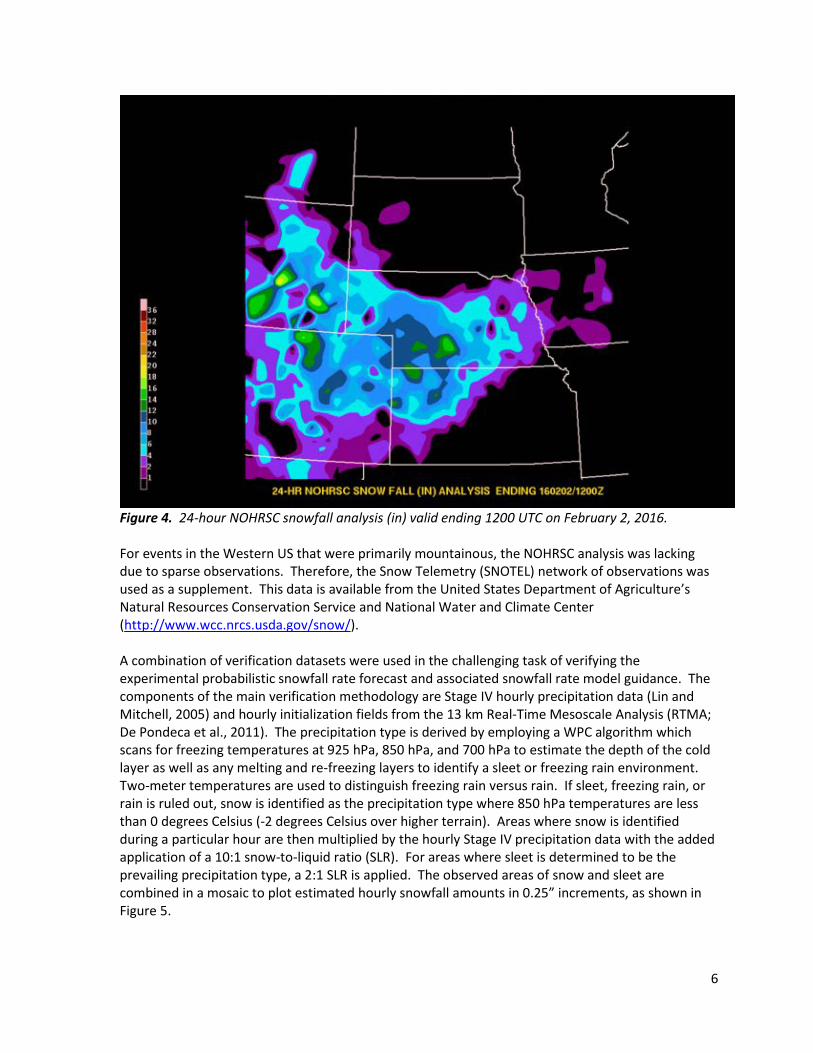
Figure 4. 24-hour NOHRSC snowfall analysis (in) valid ending 1200 UTC on February 2, 2016. For events in the Western US that were primarily mountainous, the NOHRSC analysis was lacking due to sparse observations. Therefore, the Snow Telemetry (SNOTEL) network of observations was used as a supplement. This data is available from the United States Department of Agriculture’s Natural Resources Conservation Service and National Water and Climate Center (http://www.wcc.nrcs.usda.gov/snow/). A combination of verification datasets were used in the challenging task of verifying the experimental probabilistic snowfall rate forecast and associated snowfall rate model guidance. The components of the main verification methodology are Stage IV hourly precipitation data (Lin and Mitchell, 2005) and hourly initialization fields from the 13 km Real-Time Mesoscale Analysis (RTMA; De Pondeca et al., 2011). The precipitation type is derived by employing a WPC algorithm which scans for freezing temperatures at 925 hPa, 850 hPa, and 700 hPa to estimate the depth of the cold layer as well as any melting and re-freezing layers to identify a sleet or freezing rain environment. Two-meter temperatures are used to distinguish freezing rain versus rain. If sleet, freezing rain, or rain is ruled out, snow is identified as the precipitation type where 850 hPa temperatures are less than 0 degrees Celsius (-2 degrees Celsius over higher terrain). Areas where snow is identified during a particular hour are then multiplied by the hourly Stage IV precipitation data with the added application of a 10:1 snow-to-liquid ratio (SLR). For areas where sleet is determined to be the prevailing precipitation type, a 2:1 SLR is applied. The observed areas of snow and sleet are combined in a mosaic to plot estimated hourly snowfall amounts in 0.25” increments, as shown in Figure 5.

7

Figure 5. An example of the combination Stage IV/RAP analysis used to verify hourly snowfall rates valid at 1800 UTC on February 5, 2016. The color scale for the shaded values is on the left and begins at .10 inch per hour (yellow). Radar reflectivity and METAR reports from stations that were within the probability contours drawn in the snowfall rate forecast were also used during verification. Complimentary observations such as dBZ readings from the radar reflectivity, as well as reports of snowfall and visibility from the hourly METAR reports were used to score forecasts over the specified time period. Iowa Emergency Management (IEM) in partnership with Iowa State University and the National Weather Service (NWS) has created a web-based database of NWS Local Storm Reports (LSRs) and Storm-Based Warnings (SBWs). This application allows the quick viewing of LSRs and SBWs issued by local NWS forecast offices for their area of responsibility (https://mesonet.agron.iastate.edu/lsr/). This flexible archive was a useful supplement to the verification resources utilized in the 2016 WWE.

Model Data The full multi-center suite of deterministic and ensemble guidance was available to WPC forecasters, as well as different experimental snowfall forecasting data. Table 1 summarizes the model guidance that served as the focus of the deterministic snowfall and probabilistic snowfall rate forecasts. More information about each dataset is provided below.

8

Table 1. Featured guidance for the 2016 HMT-WPC Winter Weather Experiment. Experimental guidance is shaded.

Provider Model Resolution Forecast

Hours Notes

EMC NAM Nest 4 km 60 The operational NAM Nest is a higher resolution nest of the 12 km parent NAM

EMC SREF

(26 members)

16 km

(32 km display) 87

Two dynamical cores (ARW and NMMB, 13 members each); Vertical resolution from 35-40 levels, mostly in the PBL; greater diversity in model initial conditions, perturbations, physics

EMC GEFS

(21 members) 55 km 168

Semi-Langrangian; GSI/EnKF hybrid analysis; vertical resolution of 64 levels

WPC PWPF ensemble

(68 members) 20 km 72

Operational PWPF ensemble includes the WPC deterministic forecast, SREF members, GFS mean, ECMWF mean, and deterministic NAM, GFS, CMC, and ECMWF; SLR is an average of multiple techniques

EMC NAMX 3 km 84 3 km CONUS and 3 km Alaska nest

ESRL

HRRR-TLE (high-resolution time-

lagged ensemble)

3 km 12 Neighborhood ensembling approach calculated over a 3 km grid of time-lagged HRRR deterministic members

ESRL HRRRX 3 km 24 Deterministic Experimental HRRR

WPC HRAM3E Ensemble

5 km 36 WPC multiplicative dynamic downscaling adjustment to hi-res multi-model ensemble

WPC HRAM3G

Ensemble 5 km 36

WPC multiplicative dynamic downscaling adjustment to hi-res multi-model ensemble

9

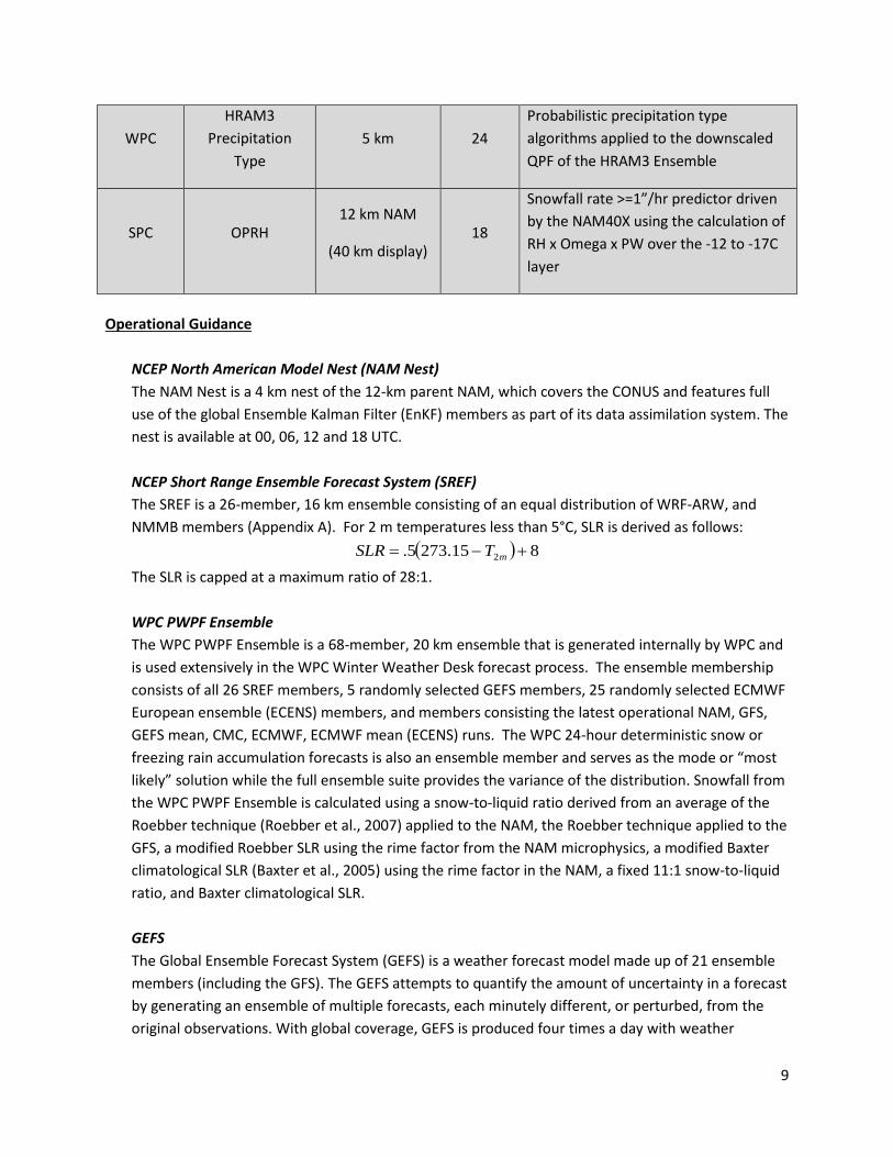
WPC HRAM3

Precipitation Type

5 km 24 Probabilistic precipitation type algorithms applied to the downscaled QPF of the HRAM3 Ensemble

SPC OPRH 12 km NAM

(40 km display) 18

Snowfall rate >=1”/hr predictor driven by the NAM40X using the calculation of RH x Omega x PW over the -12 to -17C layer

Operational Guidance

NCEP North American Model Nest (NAM Nest) The NAM Nest is a 4 km nest of the 12-km parent NAM, which covers the CONUS and features full use of the global Ensemble Kalman Filter (EnKF) members as part of its data assimilation system. The nest is available at 00, 06, 12 and 18 UTC. NCEP Short Range Ensemble Forecast System (SREF) The SREF is a 26-member, 16 km ensemble consisting of an equal distribution of WRF-ARW, and NMMB members (Appendix A). For 2 m temperatures less than 5°C, SLR is derived as follows:

( ) 815.2735. 2 +−= mTSLR

The SLR is capped at a maximum ratio of 28:1. WPC PWPF Ensemble The WPC PWPF Ensemble is a 68-member, 20 km ensemble that is generated internally by WPC and is used extensively in the WPC Winter Weather Desk forecast process. The ensemble membership consists of all 26 SREF members, 5 randomly selected GEFS members, 25 randomly selected ECMWF European ensemble (ECENS) members, and members consisting the latest operational NAM, GFS, GEFS mean, CMC, ECMWF, ECMWF mean (ECENS) runs. The WPC 24-hour deterministic snow or freezing rain accumulation forecasts is also an ensemble member and serves as the mode or “most likely” solution while the full ensemble suite provides the variance of the distribution. Snowfall from the WPC PWPF Ensemble is calculated using a snow-to-liquid ratio derived from an average of the Roebber technique (Roebber et al., 2007) applied to the NAM, the Roebber technique applied to the GFS, a modified Roebber SLR using the rime factor from the NAM microphysics, a modified Baxter climatological SLR (Baxter et al., 2005) using the rime factor in the NAM, a fixed 11:1 snow-to-liquid ratio, and Baxter climatological SLR. GEFS The Global Ensemble Forecast System (GEFS) is a weather forecast model made up of 21 ensemble members (including the GFS). The GEFS attempts to quantify the amount of uncertainty in a forecast by generating an ensemble of multiple forecasts, each minutely different, or perturbed, from the original observations. With global coverage, GEFS is produced four times a day with weather

10

forecasts going out to 16 days. The GEFS is a Semi-Langrangian model with a horizontal resolution of 55 km from 0-168 forecast hours. GEFS has 64 hybrid levels in its vertical resolution to match the GSI/EnKF hybrid analysis system. Experimental Guidance SPC OPRH Snowfall Rate Technique During the past several winters, the Storm Prediction Center (SPC), which is responsible for issuing the winter Mesoscale Discussion for heavy snow, has been utilizing a simple ingredient-based technique for identifying areas in which snowfall rates may exceed 1” per hour within the forecast period. SPC forecasters have found anecdotal correspondence between the absolute magnitude of OPRH values and hourly snowfall rates (- 1 OPRH value ≈ 1” per hr; –2 OPRH value ≈ 2” per hr). OPRH strives to physically represent processes involved in heavy snowfall rates [i.e., dendritic growth and upward vertical motion within a favorable layer]. The technique can be applied to any model. During the WWE, OPRH was applied to the 12km NAM, then displayed on a 40km projection. Below is an explanation of the OPRH calculation:

• The temperature is checked at every 25 hPa to determine when it falls between -12 and -17C.

• If that a grid point satisfies that criterion, the PW (in) is calculated (based on the mixing ratio) for that 25-mb layer.

• The RH (0-1.00) and omega (microbars/s) for that level are then multiplied together. The sum of this product is taken for each level between -12 and -17C.

• Finally, the average product of RH x omega is multiplied by the PW over the -12 to -17C layer to get OPRH.

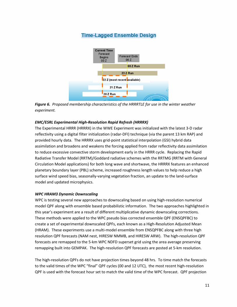
EMC NAMX The NAM Nest resolution increased from 4km in the operational NAM Nest to 3km. Snowfall rates were derived by multiplying the instantaneous one-hour precipitation rate * the instantaneous fraction of frozen precipitation * a 10:1 SLR. The 00Z cycle of the NAMX was available each day. EMC/ESRL HRRR-TLE A preliminary version of the HRRR-TLE was provided by ESRL for use in the experiment. This CONUS version of the ensemble featured a 3 km resolution, and used 3-5 time-lagged HRRR initializations to predict the probability of hourly snow fall exceeding specified accumulation thresholds. A schematic of how the system works can be found in Figure 6. The HRRR uses Thompson physics and applies a standard 10:1 snow-liquid ratio for calculating snowfall rate.

11

Figure 6. Proposed membership characteristics of the HRRRTLE for use in the winter weather experiment. EMC/ESRL Experimental High-Resolution Rapid Refresh (HRRRX) The Experimental HRRR (HRRRX) in the WWE Experiment was initialized with the latest 3-D radar reflectivity using a digital filter initialization (radar-DFI) technique (via the parent 13 km RAP) and provided hourly data. The HRRRX uses grid-point statistical interpolation (GSI) hybrid data assimilation and broadens and weakens the forcing applied from radar reflectivity data assimilation to reduce excessive convective storm development early in the HRRR cycle. Replacing the Rapid Radiative Transfer Model (RRTM)/Goddard radiative schemes with the RRTMG (RRTM with General Circulation Model applications) for both long wave and shortwave, the HRRRX features an enhanced planetary boundary layer (PBL) scheme, increased roughness length values to help reduce a high surface wind speed bias, seasonally-varying vegetation fraction, an update to the land-surface model and updated microphysics. WPC HRAM3 Dynamic Downscaling WPC is testing several new approaches to downscaling based on using high-resolution numerical model QPF along with ensemble based probabilistic information. The two approaches highlighted in this year’s experiment are a result of different multiplicative dynamic downscaling corrections. These methods were applied to the WPC pseudo bias corrected ensemble QPF (ENSQPFBC) to create a set of experimental downscaled QPFs, each known as a High-Resolution Adjusted Mean (HRAM). These experiments use a multi-model ensemble from ENSQPFBC along with three high resolution QPF forecasts (NAM nest, HIRESW NMMB, and HIRESW ARW). The high-resolution QPF forecasts are remapped to the 5-km WPC NDFD superset grid using the area average preserving remapping built into GEMPAK. The high-resolution QPF forecasts are posted at 5-km resolution. The high-resolution QPFs do not have projection times beyond 48 hrs. To time match the forecasts to the valid times of the WPC “final” QPF cycles (00 and 12 UTC), the most recent high-resolution QPF is used with the forecast hour set to match the valid time of the WPC forecast. QPF projection

12

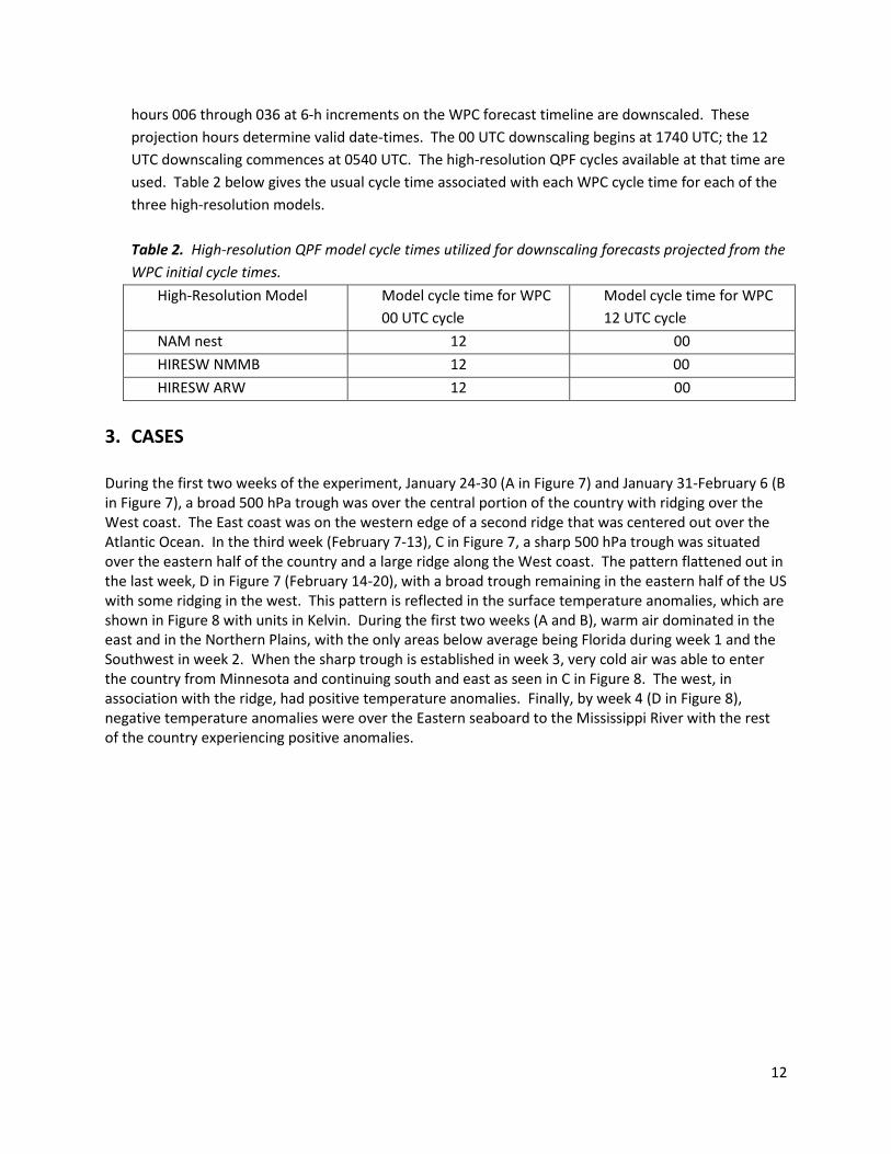
hours 006 through 036 at 6-h increments on the WPC forecast timeline are downscaled. These projection hours determine valid date-times. The 00 UTC downscaling begins at 1740 UTC; the 12 UTC downscaling commences at 0540 UTC. The high-resolution QPF cycles available at that time are used. Table 2 below gives the usual cycle time associated with each WPC cycle time for each of the three high-resolution models. Table 2. High-resolution QPF model cycle times utilized for downscaling forecasts projected from the WPC initial cycle times.

High-Resolution Model Model cycle time for WPC 00 UTC cycle

Model cycle time for WPC 12 UTC cycle

NAM nest 12 00 HIRESW NMMB 12 00 HIRESW ARW 12 00

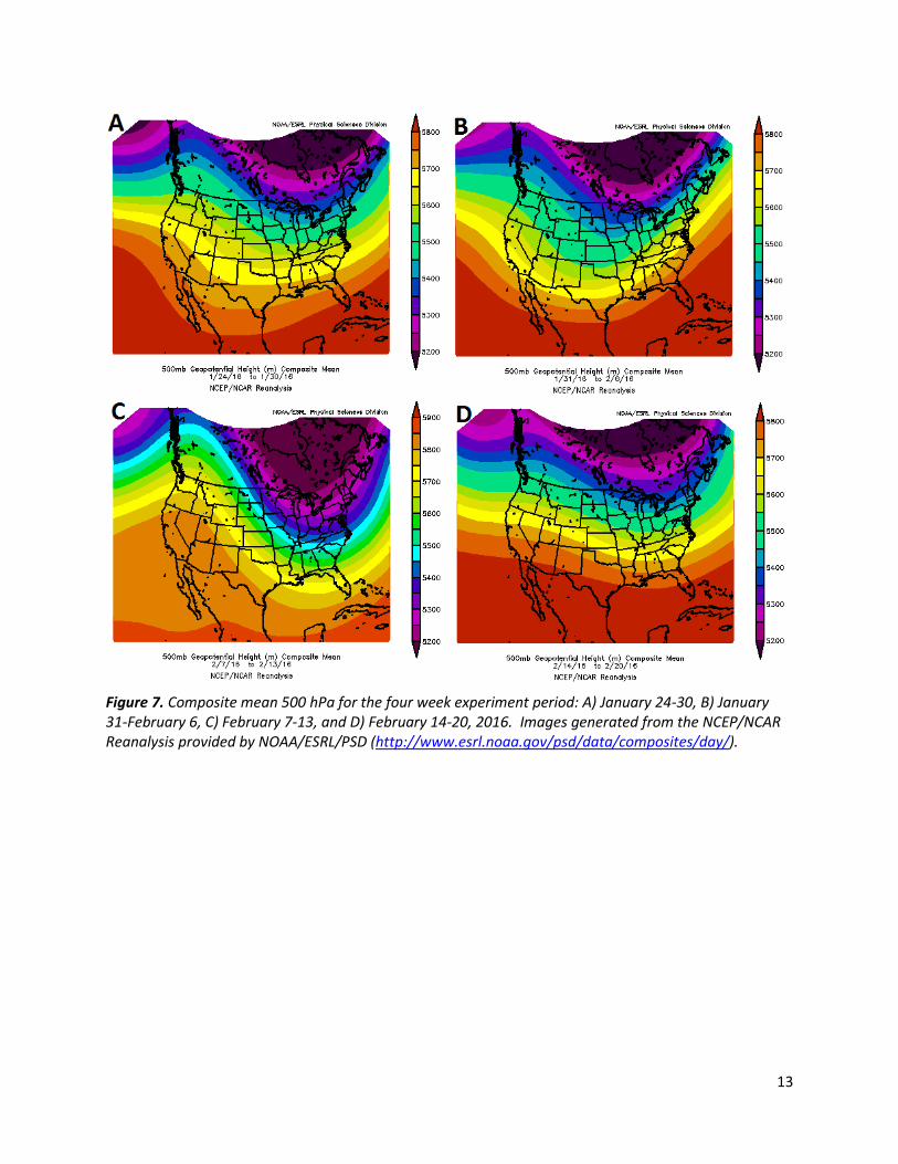
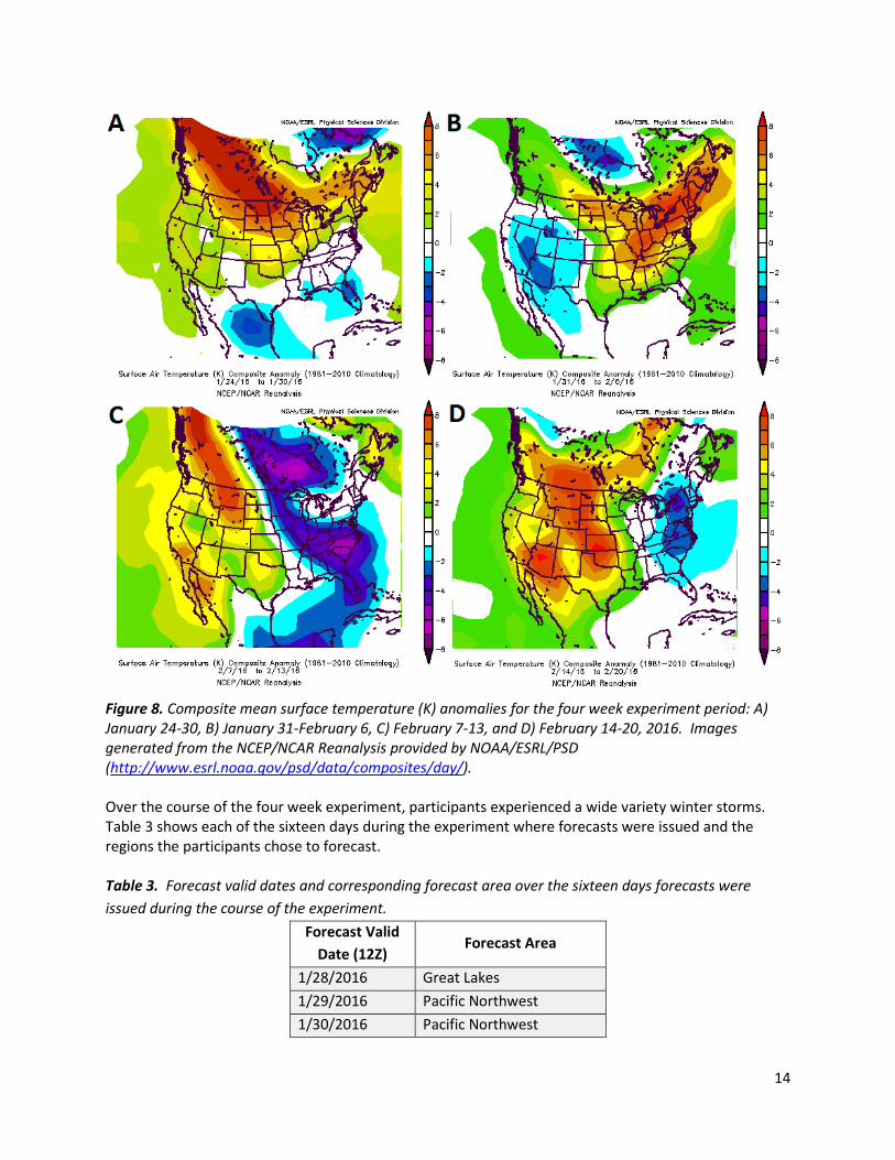
3. CASES During the first two weeks of the experiment, January 24-30 (A in Figure 7) and January 31-February 6 (B in Figure 7), a broad 500 hPa trough was over the central portion of the country with ridging over the West coast. The East coast was on the western edge of a second ridge that was centered out over the Atlantic Ocean. In the third week (February 7-13), C in Figure 7, a sharp 500 hPa trough was situated over the eastern half of the country and a large ridge along the West coast. The pattern flattened out in the last week, D in Figure 7 (February 14-20), with a broad trough remaining in the eastern half of the US with some ridging in the west. This pattern is reflected in the surface temperature anomalies, which are shown in Figure 8 with units in Kelvin. During the first two weeks (A and B), warm air dominated in the east and in the Northern Plains, with the only areas below average being Florida during week 1 and the Southwest in week 2. When the sharp trough is established in week 3, very cold air was able to enter the country from Minnesota and continuing south and east as seen in C in Figure 8. The west, in association with the ridge, had positive temperature anomalies. Finally, by week 4 (D in Figure 8), negative temperature anomalies were over the Eastern seaboard to the Mississippi River with the rest of the country experiencing positive anomalies.

13

Figure 7. Composite mean 500 hPa for the four week experiment period: A) January 24-30, B) January 31-February 6, C) February 7-13, and D) February 14-20, 2016. Images generated from the NCEP/NCAR Reanalysis provided by NOAA/ESRL/PSD (http://www.esrl.noaa.gov/psd/data/composites/day/).

14

Figure 8. Composite mean surface temperature (K) anomalies for the four week experiment period: A) January 24-30, B) January 31-February 6, C) February 7-13, and D) February 14-20, 2016. Images generated from the NCEP/NCAR Reanalysis provided by NOAA/ESRL/PSD (http://www.esrl.noaa.gov/psd/data/composites/day/). Over the course of the four week experiment, participants experienced a wide variety winter storms. Table 3 shows each of the sixteen days during the experiment where forecasts were issued and the regions the participants chose to forecast. Table 3. Forecast valid dates and corresponding forecast area over the sixteen days forecasts were issued during the course of the experiment.

Forecast Valid Date (12Z)

Forecast Area

1/28/2016 Great Lakes 1/29/2016 Pacific Northwest 1/30/2016 Pacific Northwest

15

2/2/2016 Front Range of the Rockies/Central Plains

2/3/2016 Central Plains 2/4/2016 New Hampshire/Maine 2/5/2016 New England 2/6/2016 Northeast 2/9/2016 New England 2/10/2016 Lakes, Mid-Atlantic

2/11/2016 Upper Plains, Lakes, Appalachians

2/12/2016 Upper Plains, Lakes, Appalachians

2/13/2016 Lakes, Appalachians, North Carolina

2/17/2016 New York/Lake Ontario 2/18/2016 Sierras 2/20/2016 Pacific Northwest

During the first week, the highlights were a weak clipper system that dropped down through the Upper Great Lakes and snow in the Pacific Northwest associated with atmospheric river driven storms. The beginning of the second week featured a strong storm affecting the front range of the Rockies and moving through the Central Plains. The focus then shifted to New England where a coastal storm spread snow over coastal New England on February 6. During the third week, where the coldest air was in place over the eastern part of the country, participants had lake-effect snow events almost daily. Two weaker storm systems also affected the Mid-Atlantic on February 10 and coastal North Carolina on February 13. Finally, during the fourth week, a strong storm tracked north along the Appalachian Mountains on February 17 spreading a swath of snow to the north and west of the mountains. On February 18, the participants made a retrospective forecast using an archived case study featuring the storm that impacted the Mid-Atlantic over the President’s Day holiday on February 15-16. The last two days of the experiment were spent back out west in the Sierra Nevada and in the Pacific Northwest. 4. EXPERIMENTAL DETERMINISITIC SNOWFALL FORECAST During experiment operations, 15 short-range deterministic forecasts were created. Through a combination of subjective evaluations completed during and after the experiment, all 15 forecasts were evaluated during verification using the NOHRSC snowfall analysis (supplemented with SNOTEL reports for the west). Figure 9 shows the total of scores per scoring option of the experimental snowfall forecasts. On a scale of 1 to 5, the average score overall was 3.4, with one forecast scoring a top score of 5. The comments were divided on forecast being either underdone or overdone with respect to the contours not entirely capturing the spatial extent of the snow event and/or amounts. Participants also tended to struggle at capturing forecast detail in areas of steep gradients between heavier and lighter amounts of snow.

16

Figure 9. Subjective scores assigned to the experimental deterministic snowfall forecasts created during the 2016 WWE. The forecasts were rated on a scale of 1 (Very Poor) to 5 (Very Good) Experimental HRAM3G and HRAM3E Ensemble: 24-hour Snowfall Accumulation Two of the HRAM3 downscaled ensembles run internally at WPC, the G and the E versions, were used to provide 24-hour snowfall guidance for the deterministic forecast exercise. The 24-hour snowfall was derived by masking the downscaled QPF from each respective HRAM ensemble with a weighted percentage for snow and sleet, then applying a 10:1 SLR for areas of snow, and a 2:1 SLR for sleet. Separate forecasts were generating for freezing rain by masking the downscaled QPF with the weighted percentage of freezing rain. The weighted percentages of precipitation type were computed from the hourly dominant precipitation type fields in the NAM NEST, HIRES ARW, and HIRES NMMB. An example of the output is shown in Figure 10. Participants noted that the HRAM3G and HRAM3E performed exceptionally well over the complex terrain in the western US with the downscaling significantly improving the high snowfall amounts generated by its deterministic members. It also served as very useful guidance in the Central Plains, New England, and Appalachian Mountains. However, the HRAM3E and the HRAM3G forecast snowfall amounts too light at times over the Great Lakes region for several events. The over-reduction of

17

snowfall may have been attributed to the 10:1 SLR used in deriving the forecast snowfall, thereby not accounting for the very cold environment where higher SLR values were likely. Another possible explanation for under forecasting the lake effect snowfall may be related to the narrow geometry of the snowfall bands, and variability in the location of the streamers in each of the 3 members of the ensemble. These conditions could have been over-smoothed the QPF during the downscaling process. The loss of detail maxima around the Great Lakes also tended to cause forecasters to under-forecast snowfall amounts.

Figure 10. An example of the HRAM3G (a) and HRAM3E (b) Ensembles accumulated 24-hour snowfall shown aside the deterministic snowfall forecast (c) created valid 12Z-12Z on 2/2/2016. Participants rated the HRAM3E an average score of 3.18 out of 5, which was marginally better than the HRAM3G, which received an average score of 3.06. Figure 11 shows the total of scores per scoring option for both the HRAM3E and the HRAM3G. Participants noted that the HRAM3E performed slightly better on magnitude and spatial extent of precipitation.

a) b)

c)

18

Figure 11. Subjective ratings of the HRAM3G and HRAM3E Ensembles for accumulated snowfall. The products were rated on a scale of 1 (Very Poor) to 5 (Very Good) 24-hour Change in Snow Depth Products Forecasts of 24-hour change in snow depth were used as guidance in forecast exercises, and evaluated for performance in the visual verification session each day. Two experimental models (NAMX, HRRRX), and two operational (NAM 12km, GFS) were featured. Figure 12 shows an example of the change in snow depth products along with the verification sources. Participants noted concerns regarding the utility using this field as guidance in snowfall accumulation forecasts because of the snowfall followed by melting potential over a region during the 24-hour period. The use of this field in a shorter 6-hour forecast period may make it easier to discern when snow accumulation and/or melting actually occurred. Forecasters suggested that the change in snow depth may be valuable in determining where snow may have fell and melted in areas where observational data is scarce.

19

Figure 12. An example of the NOHRSC (a) and First Energy (b) 24-hour snowfall analyses with the change in snow depth products from the HRRRX (c), NAMX (d), GFS (e), and NAM(f) models presented during subjective verification. Shaded regions in (c)-(f) show accumulating snow whereas the brown contours in (e) and (f) show areas where melting is occurring Figure 13 shows all the subjective scores given to all four products. The HRRRX was available for only 7 out of the 17 forecast days during the experiment. Participants noted over those 7 runs that the HRRRX typically under-forecast snowfall magnitude and spatial extent. The NAMX was the preferred solution based on how well it captured the coverage and magnitude of the precipitation with participants noting the “realistic” representation of streamers and bands with Lake Effect snows often being good enough to use as a first-guess when drawing contours for the snowfall forecast. The operational 12-km NAM change in snow depth product performed fairly well in capturing location and magnitude. The 27-km GFS received the poorest rating. Both lower-resolution models had difficulty over the Great Lakes and the west but were able to convey “general idea” of the snow event. It was suggested that higher performance of the models with respect to the transition of snow accumulation to melting were attributed to differences in the land surface models.

a) c)

e)

b) d) f)

20

Figure 13. Subjective ratings of the change in snow depth products from the HRRRX, NAMX, NAM, and GFS models. The products were rated on a scale of 1 (Very Poor) to 5 (Very Good).

5. EXPERIMENTAL PROBABILISTIC SNOWFALL RATE FORECAST AND GUIDANCE Participants were asked to use a suite of experimental guidance to produce a probabilistic snowfall rate forecast. Each day a threshold of 0.5, 1, or 2 inches per hour was chosen and then probability contours of 25, 50, and 75% were drawn to indicate the likelihood of the chosen snowfall rate. In addition to the probability contours, forecasters were asked to specify a time range during which the activity was most likely to occur. Over the course of the experiment, a total of fifteen experimental probabilistic snowfall rate forecasts were created and scored. Participants rated each probabilistic snowfall rate forecast subjectively each day on a scale of 0-5, ranging from very poor (1) to very good (5) and 0 for missing or forecasts that could not be scored due to a lack of verification. These ratings were based on how well both the probability contours captured the observed snowfall rates and if the observed rates occurred during the specified time period. Participants were able to forecast for any time window during the Day 1 period (first 24 hours). Over the course of the experiment, the average length of the probabilistic snowfall rate forecasts was five hours. Figure 14 displays how each probabilistic snowfall rate forecast was evaluated over the course of the experiment.

21

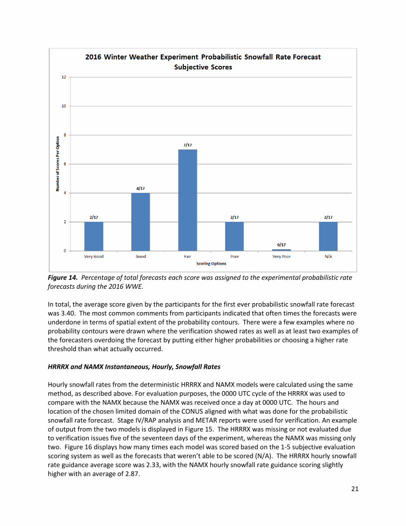
Figure 14. Percentage of total forecasts each score was assigned to the experimental probabilistic rate forecasts during the 2016 WWE. In total, the average score given by the participants for the first ever probabilistic snowfall rate forecast was 3.40. The most common comments from participants indicated that often times the forecasts were underdone in terms of spatial extent of the probability contours. There were a few examples where no probability contours were drawn where the verification showed rates as well as at least two examples of the forecasters overdoing the forecast by putting either higher probabilities or choosing a higher rate threshold than what actually occurred. HRRRX and NAMX Instantaneous, Hourly, Snowfall Rates Hourly snowfall rates from the deterministic HRRRX and NAMX models were calculated using the same method, as described above. For evaluation purposes, the 0000 UTC cycle of the HRRRX was used to compare with the NAMX because the NAMX was received once a day at 0000 UTC. The hours and location of the chosen limited domain of the CONUS aligned with what was done for the probabilistic snowfall rate forecast. Stage IV/RAP analysis and METAR reports were used for verification. An example of output from the two models is displayed in Figure 15. The HRRRX was missing or not evaluated due to verification issues five of the seventeen days of the experiment, whereas the NAMX was missing only two. Figure 16 displays how many times each model was scored based on the 1-5 subjective evaluation scoring system as well as the forecasts that weren’t able to be scored (N/A). The HRRRX hourly snowfall rate guidance average score was 2.33, with the NAMX hourly snowfall rate guidance scoring slightly higher with an average of 2.87.

22

Figure 15. Hourly snowfall rates from the HRRRX (A) and the NAMX (B) valid at 1800 UTC on February 5, 2016. Shaded values are in inches per hour.

Figure 16. The subjective evaluation ratings for the snowfall rate guidance from the deterministic HRRRX and NAMX models during the 2016 WWE.

23

The most common response about the guidance was that the rates in the models were often too light in intensity and underdone in areal coverage. The snowfall rate algorithm struggled the most around the Great Lakes region, highlighted during the third week of the experiment when there were many lake-effect snow events. However, they did show some promise in picking up narrow bands and streamers coming off the lakes. A possible reason for the underperformance in the lake-effect snow cases is thought to be at least partially attributed to the 10:1 SLR used in the algorithm for calculating the snowfall rate. Often in lake-effect events and other events with very cold air, SLR’s tend to be higher than 10:1. Because of this problem during the third week, an experimental version of the NAMX snowfall rate algorithm was made available using a Baxter SLR climatology values (Baxter et al., 2005). These rates were not formally evaluated with scores, however received positive feedback from the forecasters as they did show heavier rates in the lake-effect situations than the rate algorithm using the 10:1 SLR. Despite the problems at times in handling the intensity and areal coverage of the snow bands, participants overall had positive comments in regards to forecasting snowfall rates and were impressed having seen the data for the first time in this format. Many forecasters from WFOs stated that snowfall rate information is something that is often requested by their users and having that information is very beneficial to the impacts-based forecast they are providing to the public and their other partners. Because of the positive reception, it is suggested that work on the snowfall rate guidance and algorithms should continue. One suggestion for future work is to adjust the SLR within the calculation from a static 10:1 to either the Baxter climatological SLR or perhaps a blended SLR. Another possible improvement is to simply focus on hourly snowfall derived continuously from the model. Participants also expressed a desire for the maximum snowfall rate over the course of the entire hour. Many thought this information would be much more useful in trying to discern snowfall rates for a forecast rather than just an instantaneous value at the top of every hour. HRRR Time-Lagged Ensemble Probabilistic Snowfall Rates The HRRR Time-Lagged Ensemble was used and subjectively evaluated in the 2016 Winter Weather Experiment. The HRRR-TLE provided probabilistic snowfall rate guidance every hour, when available, out to twelve hours for three different rate thresholds: 0.5, 1 and 2 inches of snow per hour. Although all three thresholds were available for guidance to make a forecast, only the half inch and one inch thresholds were subjectively evaluated and assigned scores. An example of the HRRR-TLE half and one inch probability thresholds are displayed in Figure 17. Each threshold was evaluated over the same domain and time length of the probabilistic snowfall rate forecast and were one hour in length. For example, if 1800 UTC was being evaluated, the one hour forecast from the 1700 UTC HRRR-TLE run was used. Stage IV/RAP analysis and METAR reports were used for verification. Figure 18 shows a

24

breakdown of how the half and one inch thresholds were scored over the course of the experiment.

Figure 17. Probabilities of half-inch per hour (A) and one-inch per hour (B) snowfall rates from the HRRR-TLE valid at 1500 UTC on February 2, 2016. Probabilities are shaded beginning at 5% as the dark purple and increasing in 5% intervals to 95%. Six forecasts were unable to be scored due to missing data or lack of verification resources. The average score given to the half inch per hour threshold was 2.64 out of 5. The inch per hour threshold had a higher average score of 3.18 out of 5. Similar to the deterministic products, participants noted that the probabilities were frequently on the low side in terms of both magnitude and areal coverage; however the areal extent of the data was often correct. The higher average rating for the one inch per hour threshold can be attributed to a few cases when the participants ranked it more favorably when it did not have any false alarms. This occurred several times when the probabilities of an inch per hour were either zero or very low and the associated verification showed no snowfall rates that reached an inch per hour.

25

Figure 18. The subjective evaluation ratings for the snowfall rate guidance for the probability of 0.5 and 1 inch per hour snowfall rates from the HRRR-TLE model during the 2016 WWE. The HRRR-TLE also experienced problems handling lake-effect events around the Great Lakes. First, it uses an 80 km spatial filter where it treats forecasts at all grid points in an 80-km radius around a given point as ensemble “members”. A radius this large prevented the HRRR-TLE from being able to capture geographically-narrow lake-effect streams and convective bands around the Great Lakes region. Also, due to the deterministic HRRR members continuous snowfall accumulation, which is an actual estimate of snow accumulation using frozen hydrometeors generated via the microphysics minus the snow-melt from land use, there can be no measured snowfall over the lake waters. This frequently caused lower probabilities to be clustered around the periphery of the lake which could be misleading to forecasters expecting to see a more continuous signal over the lake. Much like the HRRRX and NAMX, despite some of the HRRR-TLE’s shortcomings, the majority of the participants had an overall positive opinion of the model and they were encouraged by the availability of this data. Many participants agreed that the forecast time of 12 hours was too short to have any impact on the watch/warning process in a typical WFO. However, for short-term forecasts and smaller, localized warning or advisory products that are issued in the near term, many felt that the HRRR-TLE would be very valuable guidance. Participants also liked having high resolution, probabilistic information to aid in determining confidence when forecasting different events. Based on this feedback, it is suggested that work continues to try and improve the snowfall rate probabilities. The

26

most prevalent suggestion is to create a smaller, varying spatial filter over the Great Lakes for lake-effect events. This would also prove beneficial in mountainous areas. OPRH Snowfall Rate Technique Participants were asked to subjectively evaluate the OPRH technique each day. One hour within the time range of the probabilistic snowfall rate forecast was chosen for evaluation each day. Stage IV/RAP analysis, radar reflectivity, and METAR reports were used for verification. An example of the OPRH technique is shown in Figure 19.

Figure 19. The OPRH technique valid at 1800 UTC on February 5, 2016. The dashed purple lines represent a -0.5 OPRH value which equates to a half inch per hour snowfall rate. The shaded values span from -1.0 to -3.0, or one inch per hour to three inches per hour. The scores assigned to the OPRH technique are shown in Figure 20. There was only one day where there was not suitable verification to score and out of sixteen total scores, twelve ranked either “fair” or “good.” The average score over the course of the experiment was 3.19.

27

Figure 20. The subjective evaluation ratings for the snowfall rate guidance for the OPRH technique during the 2016 WWE. The OPRH technique received mostly positive feedback from the participants. Although limited to just seeing one hour each day for verification, many noted that the tool did well in identifying the location and often times magnitude of the snowfall rates that verified. At times it was considered to be underdone, which was also a common criticism with the model guidance for snowfall rates. A concern with the technique is that the forecast snowfall rates are independent of the model precipitation forecast. This resulted in instances where the tool heightened awareness for hourly snowfall rates to impact the forecast; however no precipitation was forecast or observed. Moreover snowfall rates were triggered in areas where the precipitation type was sleet or rain. A suggestion for future work on this technique would be to add a check for precipitation-type and mask out precipitation types other than snow. The OPRH technique is also limited in scenarios where the optimum dendritic growth layer is shallow or above the optimum vertical motion. A closely related problem that was also frequently noted in cases was when strong orographic lift was present. Orographic lift is not always accounted for in the OPRH algorithm, and the lift over complex terrain areas often did not align with the optimum dendritic layer. 6. DAY 2 OR 3 PROBABILISTIC WINTER HAZARDS PRODUCT The afternoon activity featured the creation of a winter hazards depiction addressing impactful winter weather and its predictability. This was a free form drawing using plain language, assorted contours and

28

labeling, and the option of numerical probabilities. Participants started with the 30% probability of meeting or exceeding the 24-hour WFO thresholds for issuing a winter storm watch as produced by the Watch Collaborator. They were then encouraged to use an array of probabilistic guidance and reforecast tools to assess the predictability of snow, ice, wind, and precipitation transition zones to create a product that provides more information to the user than simply meeting legacy impact thresholds (Figure 21).

Figure 21. An example of a Day 2 Winter Hazards Product (valid 2/3/2016) produced during the 2016 WWE afternoon activity. For this example, hazardous weather was indicated using contours and labeling. Filled contours depicted areas of higher probability of hazard impact. The creation of this product drew upon the use of Global Ensemble Forecast System (GEFS) reforecast data for probabilistic QPF thresholds, and several experimental tools developed at WPC. These experimental tools included WPC PWPF data in 6-hour increments to assess the potential for impacting snow and freezing rain in a shorter time period, and the probability of NDFD surface winds exceeding significant thresholds (such as those used for blizzard conditions). The tools were developed to better assess the predictability of winter hazards, more finely identify impactful winter weather, and identify multiple threats over a specific region. The ultimate goal is to improve the operational Watch Collaborator and enhance public-facing products such as the National Forecast Chart. Overall, the synoptic features and impacts were considered well-forecast for Days 2 and 3 outlooks.

Much discussion regarding probabilistic forecasting and impacts-based messaging surrounded the development of this product each day. Frequent feedback and commentary included that more winter-focused probabilistic guidance and tools are needed at longer ranges to improve probabilistic

29

forecasting, and that impacts-based messaging should attempt to reduce ambiguity thus increasing confidence. Awareness of the product user is needed when applying these terms (i.e. decision support or hazards outlook).

7. WATCH COLLABORATOR

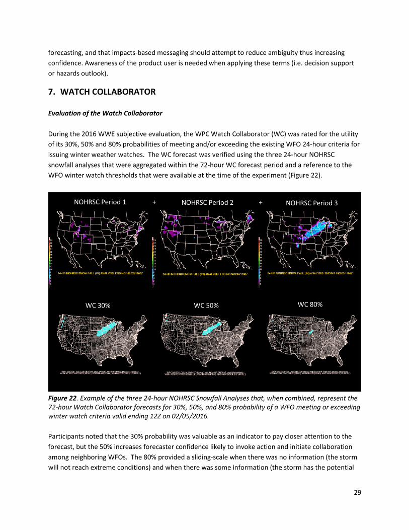
Evaluation of the Watch Collaborator During the 2016 WWE subjective evaluation, the WPC Watch Collaborator (WC) was rated for the utility of its 30%, 50% and 80% probabilities of meeting and/or exceeding the existing WFO 24-hour criteria for issuing winter weather watches. The WC forecast was verified using the three 24-hour NOHRSC snowfall analyses that were aggregated within the 72-hour WC forecast period and a reference to the WFO winter watch thresholds that were available at the time of the experiment (Figure 22).

Figure 22. Example of the three 24-hour NOHRSC Snowfall Analyses that, when combined, represent the 72-hour Watch Collaborator forecasts for 30%, 50%, and 80% probability of a WFO meeting or exceeding winter watch criteria valid ending 12Z on 02/05/2016. Participants noted that the 30% probability was valuable as an indicator to pay closer attention to the forecast, but the 50% increases forecaster confidence likely to invoke action and initiate collaboration among neighboring WFOs. The 80% provided a sliding-scale when there was no information (the storm will not reach extreme conditions) and when there was some information (the storm has the potential

NOHRSC Period 1 NOHRSC Period 2 NOHRSC Period 3

WC 30% WC 50% WC 80%

+ +

30

to have large impacts). As an additional tool during the second two weeks of the WWE, participants were offered a difference plot that presented an easier identification of locations where the 24-hour NOHRSC analysis exceeded the WFO winter watch criteria (Figure 23). This representation increased participant understanding of the WC product.

Figure 23. Example of the three 24-hour difference of NOHRSC Snowfall Analyses and the WFO winter watch criteria that, when combined, represent the 72-hour Watch Collaborator forecasts for 30%, 50%, and 80% probability of a WFO meeting or exceeding winter watch criteria valid ending 12Z on 02/05/2016. Figure 24 shows that the average subjective rating of the WC 30% probability forecast was 3.81 out of 5, the 50% was 4 out of 5, and the 80% was 3.87 out of 5. Participants commented that the 30% should, in theory, give you the most signal and the most information. The 50% was rated highly for accuracy and utility to WFO forecasters.

Shaded Region Indicates NOHRSC exceedance of WFO 24-hour Watch Criteria

WC 30% WC 50% WC 80%

31

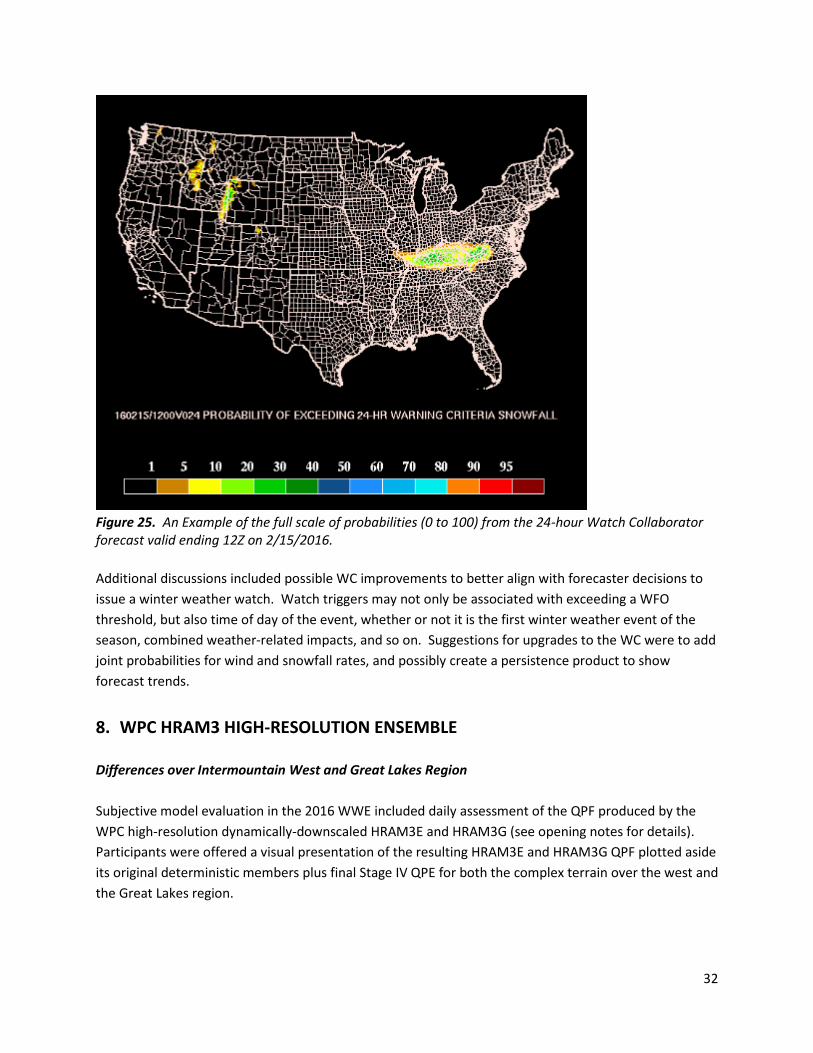
Figure 24. Average subjective ratings for each Watch Collaborator probability forecast of meeting or exceeding WFO Winter Watch Criteria. The probabilities were rated on a scale of 1 (Very Poor) to 5 (Very Good). Discussion: The Value and Future of the Watch Collaborator Participants from the WFOs were largely in agreement that there is value in the information provided by the WC. The WC has the potential to initiate collaboration among neighboring WFOs working to comply with consistency and messaging when issuing Winter Storm Watches. These forecasters unanimously expressed the desire to have all of the percentiles of the WC (Figure 25) available in the field, rather than being limited to the 30% and 50% probabilities offered to them in its current state. Participants also noted that the WPC PWPF has higher utility than the current WC because it does not account for the various impacts forecasters assess before issuing a watch. The PWPF is an ingredient to assess impacts before issuing a winter weather watch rather than a recommender. Run-to-run forecast trends for both the PWPF and the WC would be desired.

32

Figure 25. An Example of the full scale of probabilities (0 to 100) from the 24-hour Watch Collaborator forecast valid ending 12Z on 2/15/2016. Additional discussions included possible WC improvements to better align with forecaster decisions to issue a winter weather watch. Watch triggers may not only be associated with exceeding a WFO threshold, but also time of day of the event, whether or not it is the first winter weather event of the season, combined weather-related impacts, and so on. Suggestions for upgrades to the WC were to add joint probabilities for wind and snowfall rates, and possibly create a persistence product to show forecast trends.

8. WPC HRAM3 HIGH-RESOLUTION ENSEMBLE Differences over Intermountain West and Great Lakes Region Subjective model evaluation in the 2016 WWE included daily assessment of the QPF produced by the WPC high-resolution dynamically-downscaled HRAM3E and HRAM3G (see opening notes for details). Participants were offered a visual presentation of the resulting HRAM3E and HRAM3G QPF plotted aside its original deterministic members plus final Stage IV QPE for both the complex terrain over the west and the Great Lakes region.

33

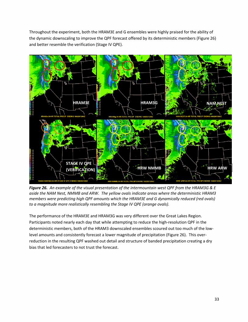
Throughout the experiment, both the HRAM3E and G ensembles were highly praised for the ability of the dynamic downscaling to improve the QPF forecast offered by its deterministic members (Figure 26) and better resemble the verification (Stage IV QPE).

Figure 26. An example of the visual presentation of the intermountain west QPF from the HRAM3G & E aside the NAM Nest, NMMB and ARW. The yellow ovals indicate areas where the deterministic HRAM3 members were predicting high QPF amounts which the HRAM3E and G dynamically reduced (red ovals) to a magnitude more realistically resembling the Stage IV QPE (orange ovals). The performance of the HRAM3E and HRAM3G was very different over the Great Lakes Region. Participants noted nearly each day that while attempting to reduce the high-resolution QPF in the deterministic members, both of the HRAM3 downscaled ensembles scoured out too much of the low-level amounts and consistently forecast a lower magnitude of precipitation (Figure 26). This over-reduction in the resulting QPF washed out detail and structure of banded precipitation creating a dry bias that led forecasters to not trust the forecast.

STAGE IV QPE (VERIFICATION)

HRAM3E HRAM3G NAM NEST

HRW ARW HRW NMMB

34

Figure 26. An example of the visual presentation of the Great Lakes QPF from the HRAM3G & E aside the NAM Nest, HRW NMMB and HRW ARW. The yellow ovals indicate areas where the deterministic HRAM3 members were predicting high QPF amounts which the HRAM3E and G over-reduced (red ovals) to a magnitude less resembling the Stage IV QPE (orange oval) than its members. Participants were content with the QPF provided by the HRAM3E and HRAM3G for all areas of the CONUS except for the Great Lakes region. Its highest utility was over the western half of the CONUS over areas of complex terrain. QPF Scoring Results During verification, participants were asked to comment on both the results over the Great Lakes and the intermountain west, but to score the QPF based on the domain that had the most weather activity (Figure 27). Of the 16 total evaluations, the HRAM3E received an average rating of 3.81, exceeding the HRAM3G average rating of 3.56. Whereas the HRAM3E and G performed very similarly with respect to areal extent, participants consistently noted that the HRAM3E better captured the magnitude of the QPF than the HRAM3G, resulting in the higher average score.

HRAM3E HRAM3G NAM NEST

HRW ARW HRW NMMB STAGE IV QPE (VERIFICATION)

35

Figure 27. The results of the 16 total subjective verification ratings of the QPF from the HRAM3E and HRAM3G during the 2016 WWE. The QPF was rated on a scale of 1 (Very Poor) to 5 (Very Good). 9. SUMMARY

The 6th annual WWE took place from January 25-February 19 at the NCWCP building in College Park. This experiment brought together 31 WFO forecasters, academic researchers, environmental modelers and social scientists to explore new model data sets and forecast tools with the goal of improving winter weather forecasting. Each day, the participants chose a weather-active area of the CONUS and used both experimental and operational guidance to create a 24-hour (Day 1) experimental deterministic snowfall forecast, one to three short-fuse experimental probabilistic snowfall rate forecasts, and a probabilistic based Day 2 or Day 3 Winter Hazards map. Participants also engaged in subjective evaluation of the experimental forecasts and guidance.

Preliminary results show that the new hourly snowfall rate parameters from the experimental high-resolution NAMX and HRRRX indicate skill in forecasting localized impactful high-intensity snow events, including the identification of lake effect streamers. Also promising are the probabilistic snowfall rate forecasts from the HRRR Time-lagged ensemble, although current spatial filters and neighborhood technique need improvement for lake effect snow forecasting. The initial exploration of these fields in the WWE, and the experiment results suggest that model developers should continue to work to

36

improve the forecast capability of these parameters. Moreover, given the demand from WFO forecasters, the snowfall rate data should be made available operationally to the field. Results from other high-resolution experimental guidance that provided 24-hour snowfall accumulation are also promising. Most noteworthy was the performance of the downscaled HRAM3 ensemble, which was well-rated by participants because of its ability to resolve QPF/snowfall detail over complex terrain such as the Sierras, Pacific Northwest, and Appalachian Mountains. Work must continue on improving these forecasts over the Great Lakes region. Lastly, the Watch Collaborator was both used as guidance and evaluated for utility. At the center of many participant discussions, it was determined that the Watch Collaborator does provide value to the WFOs for initiating collaboration on timing and placement of Winter Storm Watches. The field forecasters requested the capability to view all probabilities for thresholds of exceedance (10%-90%) rather than the currently-available 30% and 50%. It was determined that future work on improving the Watch Collaborator should include introducing joint probabilities that may factor into watch issuance such as wind and snowfall rates. Also desired is a persistence product between Watch Collaborator 12-hour predictions.

37

REFERENCES

Baxter, M. A., C. E. Graves, and J. T. Moore, 2005: A climatology of snow-to-liquid ratio for the contiguous United States. Wea. Forecasting, 20, 729-744.

De Pondeca, M. S. F. V., G. S. Manikin, G. DiMego, S. G. Benjamin, D. F. Parrish, R. J. Purser, W-S.

Wu, J. D. Horel, D. T. Myrick, Y. Lin, R. M. Aune, D. Keyser, B. Colman, G. Mann, and J. Vavra, 2011: The Real-Time Mesoscale Analysis at NOAA’s National Centers for Environmental Prediction: Current status and development. Wea. Forecasting, 26, 593-612.

Lin, Y. and K. Mitchell, 2005: The NCEP Stage II/IV hourly precipitation analyses: Development

and applications. Preprints. 19th Conf. on Hydrology, San Diego, CA., 1.2.

Roebber, P.J., Melissa R. Butt, Sarah J. Reinke, and Thomas J. Grafenauer, 2007: Real-Time Forecasting of Snowfall Using a Neural Network. Wea. Forecasting, 22, 676–684.

38

APPENDIX A

Participants

Week WPC Forecaster

WFO/National Center Research/Academia/Private Sector

EMC

January 25-29, 2016

Mary Beth Gerhardt

Pat Moore (GSP) Glen Merrill (SLC) Jeff Peters (SPC)

Phil Shafer (MDL) Curtis Alexander (ESRL

GSD)

Eric Aligo

February 1-5, 2016

Frank Pereira Ray Martin (LWX) Tom Hultquist (SOO

MPX)

Pat Market (University of Missouri)

Brian Koltz (FirstEnergy Corp.)

Isidora Jankov (ESRL GSD)

Brad Ferrier Jacob Carley

February 8-11, 2016

Dan Petersen Greg DeVoir (CTP) David Church (BUF)

Mike Montefusco (AKQ) Phil Schumacher (FSD) Marc Kavinsky (MKX)

Trevor Alcott (ESRL GSD)

February 16-19, 2016

Paul Kocin Brian D. Smith (LZK) Kevin Sullivan (JKL)

Rich Maliawaco (GGW)

Tara Jensen (UCAR DTC) Marty Baxter (Central Michigan University)

Josh Kastman (University of Missouri)

Ruiyu Sun Geoff Manikin

39

APPENDIX B

Daily Schedule

8:00am – 9:45am Determine the daily forecast area and time period (Day 1). Using 00 UTC and any available 12 UTC guidance, issue an experimental 24 hr deterministic snowfall forecast for the 12 – 12 UTC period.

9:45am – 10:00am Break

10:00am – 11:30am Additional to this forecast, probabilistically indicate areas in which snowfall rates may meet or exceed 1” per hour and when this peak may occur -OR- produce a probabilistic freezing rain forecast if no high rate events are expected.

Prepare forecast discussion.

11:30am – 12:30pm Lunch

12:30pm – 1:00pm Weather briefing to interested local WFOs

1:00pm – 2:30pm Subjective evaluation/verification

2:30pm – 2:40pm Break

2:40pm – 4:00pm Produce probabilistic Day 2 or Day 3 winter hazards impact-based product