The 11th CERThe 11th CEReeSSInternational Symposium International Symposium on on Remote SensingRemote Sensing

Satellite active and passive microwave sensing of sea ice in the Okhotsk Sea

Leonid M. Mitnik, Vyacheslav Dubina, and Maia Mitnik

V.I. Il’ichev Pacific Oceanological InstituteFar Eastern Branch, Russian Academy of Sciences

43 Baltiyskaya St., 690041, Vladivostok, RussiaPhone: 07.4232.312854, fax: 07.4232.312573 E-mail: mitnik@poi.dvo.ru

14 December 2005

Outlines

1. Introduction

2. Passive microwave sensing. Simulation of brightness temperatures over sea ice

3. Active microwave sensing

4. Sensors (SAR, ASAR, SeaWinds, AMSR, AMSR-E), supplementary satellite and in situ data

5. Sea ice on ERS-2 SAR and Envisat ASAR images

5.1. Aniva Bay

5.2. Northern and Western Okhotsk Sea

5.3. Eastern Okhotsk Sea 6. Conclusions

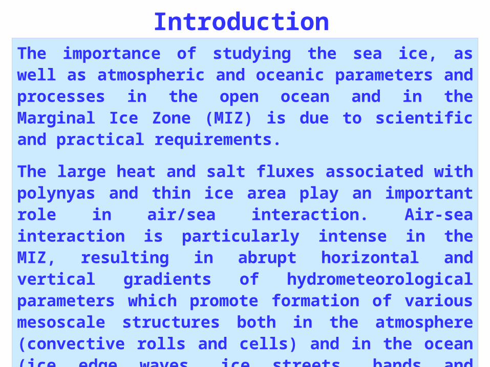
IntroductionThe importance of studying the sea ice, as well as atmospheric and oceanic parameters and processes in the open ocean and in the Marginal Ice Zone (MIZ) is due to scientific and practical requirements.

The large heat and salt fluxes associated with polynyas and thin ice area play an important role in air/sea interaction. Air-sea interaction is particularly intense in the MIZ, resulting in abrupt horizontal and vertical gradients of hydrometeorological parameters which promote formation of various mesoscale structures both in the atmosphere (convective rolls and cells) and in the ocean (ice edge waves, ice streets, bands and eddies).

Accurate estimation of their area and ice thickness will allow to improve the large-scale ice mass balance and the oceanic salt production.

Passive microwave sensingSatellite passive microwave measurements of brightness

temperatures TB() have been used for sea ice, wind speed, SST,

atmospheric water vapour content V and total cloud liquid water content Q and precipitation studies. The changes of the sea surface emissivity caused by variations of water temperature and salinity and wind action can be estimated reasonably well.

Over the compact ice cover and over marginal ice zone, variations of

TB() are due to the change of sea ice concentration C (from 0.0 to

1.0), types of sea ice, the evolution of snow/sea-ice thermophysical properties including liquid water presence in the system, snow pack density and snow grain metamorphism, air temperature and wind. V and Q retrieval presents a difficult problem due to the larger values and higher variability of the underlying surface emissivity compare to the water surface.

Simulation of the AMSR brightness temperatures

Modeling of microwave measurements over the open ocean, the MIZ and compacted ice was carried out with a microwave radiative transfer program. The program allows to compute the brightness temperatures of the underlying surface-atmosphere system TBV,H() at frequency with the vertical (V) and horizontal (H) polarizations. The radiosonde (r/s) database was built up to model atmospheric conditions observable near and over the MIZ. Total 478 r/s with SST tS  1C were selected: 69 sets from research vessels and 409 sets from 6 polar coastal and island stations. Every set consists of radiosonde, meteorological data (wind speed W and direction, forms and amount of clouds) and tS values. In the database, the water vapor content V = (0.63-18.5) kg/m2, cloud water content Q  0.25 kg/m2 and wind speed W  18.0 m/s. R/s atmospheric profiles were complimented by the cloud liquid water content profiles. For each r/s, the TBs() were computed for unifrmly distributed values

of sea ice concentration C = 0.0 - 1.0.

),(2,

),(,),(,

)],(1[

)],(1)[,(),(),(),(,

eT

eTTeTTHV

C

HVBatmBatmBocean

HVB

HV

SHVHV

Bocean TT ),(),( ,, is the brightness temperature of the under-lying surface, Ts is surface temperature .

),( BatmT is the upwelling brightness temperature of the atmosphere

),( BatmT is the downwelling brightness temperature of the atmosphere

- brightness temperature of the atmosphere-underlying surface - brightness temperature of the atmosphere-underlying surface system with vertical (system with vertical (VV) and horizontal () and horizontal (HH) polarization as a ) polarization as a function of frequency function of frequency and incidence angle and incidence angle . .

V,H(,,tS,W) is emissivityis emissivity of the surfaceof the surface

τ(,θ) is integral absorptionis integral absorption of the atmosphereof the atmosphere

Tc is brightness temperature of cosmic radiation

EmissivityFor each radiosonde, the brightness temperatures TBs() were

computed for 10 values of sea ice concentration C = 0.0 - 1.0. The emissivity of the underlying surface V,H was determined by Eq. 1 

V,H(,,tS,W) = WV,H(,,tS,W)(1 - C) + I

V,H(,, tI) C , (1) 

where W and I are sea surface and sea ice emissivity,

correspondingly, tS is sea surface temperature, W is wind speed, tI

is temperature of ice surface .

Emissivity of the calm sea surface at frequencies = 18.7, 23.8 and 36.5 GHz was computed from the Fresnel formulas [Ellison et al., Radio Sci., 1998] . Increments of emissivity associated with the wind action were found on the basis of experimental data [Rosenkranz, 1992; Sasaki et al., 1987; Wentz, 1992].

Emissivity of calm water and sea ice at = 55

Frequency, GHz (polarization)

18.7 (V/H) 23.8 (V/H) 36.5 (V/H)

Water (tS = -0.6C) [1] 0.6358/0.2825 0.6685/0.3045 0.7332/0.3524

Dark nilas [2] 0.76/0.67 0.76/0.67 0.80/0.77

Gray nilas [2] 0.84/0.80 0.85/0.82 0.88/0.84

Light nilas [2] 0.95/0.89 0.96/0.91 0.97/0.94

First-year ice (no melting) [2]Thick first-year ice [4]

0.95/0.91 0.97/0.90

0.945/0.91 0.94/0.900.97/0.90

1. Ellison et al., 1998; 2. Eppler et al., 1992; 3. Svendson et al., 1987; 4. Harouche, I.P-F. and D.G. Barber (2001)

Emissivity of new ice, nilas and water

0.2

0.3

0.4

0.5

0.6

0.7

0.8

0.9

-2 0 2 4 6 8 10 12 14

SST

Em

issi

vity

6.9H

18.7H

36.5H

89.0H

6.9V

18.7V

36.5V

89.0V

6.9H

18.7H

36.5H

89.0H

6.9V

18.7V

36.5V

89.0V

Emissivity as a function of frequency for grease ice and nilas of three different thickness ( = 50o) (left, Eppler et al., 1992 )

and water as a function of temperature at AMSR-E frequencies at V- and H-pol (right)

Emissivity of sea ice

Emissivity as a function of ice thickness at 18, 37 and 90 GHz (V-pol) for saline ice [Grenfell et al., 1988].

Brightness temperature of calm sea surface

Brightness temperature of the calm sea surface as a function of water temperature (V- and H-pol) at AMSR-E frequencies.

H

V

Spectra

Computed spectra of brightness temperature of the ocean-atmosphere system with V-pol (solid curves) and H-pol (dashed curves). Arrows mark AMSR-E frequencies.

Q (kg/m2)

V (kg/m2)

T (oC)

0.5619.3 0.34

0.2613.8 1.13

0.143.6 0.42

0.02.8-1.01

Frequency (GHz)

12

1

34

43

2

Spectra of brightness temperature

Spectra of brightness temperature over the Marginal Ice Zone

50

75

100

125

150

175

200

225

250

0 10 20 30 40 50

Frequency (GHz)

S

1

2

3

1

V

H

3

2

S=0

0< S< 30%

S=0

0< S< 30%

3

t

CV

kg/m2

Q kg/m2

1 0.6 2.8 0.0

2 0.5 9.1 0.09

3 0.0 15.6 0.17

C = 0

C = 0.3

C = 0.3

C = 0

V

H

Active microwave sensingBrightness of radar image is determined mainly by small-scale roughness and permittivity of the underlying snow-ice surface. These characteristics, in turn, are function of types of sea ice, the evolution of snow/sea-ice thermophysical properties including liquid water presence in the system, snow pack density and snow grain metamorphism, air temperature and wind.

The grease ice damps the small gravity and capillary waves due to increased viscosity and the corresponding areas look dark on SAR images. The areas with weak winds also look dark that hinders detection of the grease ice on the images.

Winds and waves are also favor to the formation of the pancake ice. It is characterized by the presence of plentiful cm-scale nonuniformities resulting in the increased backscatter. These features make possible their reliable identification.

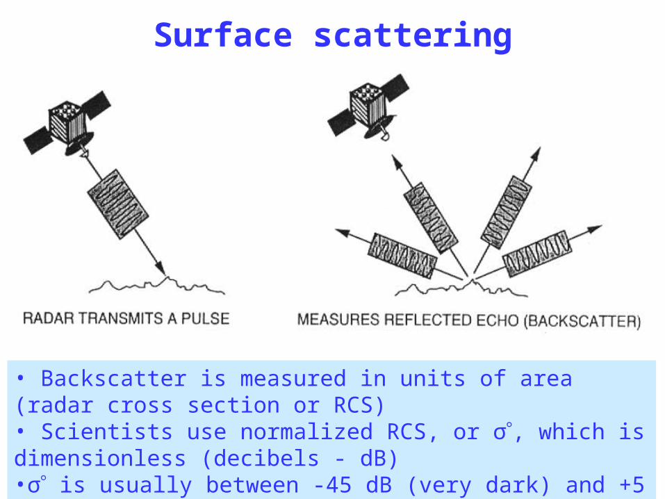
Surface scattering

• Backscatter is measured in units of area (radar cross section or RCS)• Scientists use normalized RCS, or σ, which is dimensionless (decibels - dB)•σ is usually between -45 dB (very dark) and +5 dB (very bright)

Sensors: AMSR, AMSR-E, SAR, ASAR,

SeaWinds and supplementary satellite and in situ data

Microwave radiometers

The Advanced Microwave Scanning Radiometer for EOS (AMSR-E) is a Japanese sensor that was launched on the NASA Aqua satellite in May 2002.

The AMSR, a similar instrument was launched on the Japan ADEOS-II satellite in December 2002. AMSR has about twice the spatial resolution of SSM/I with resolution as low as 5 km at frequency of 89.0 GHz. This is a substantial improvement over SSM/I and yields improved benefits from passive microwave imagery both over the ice-free sea and ice areas.

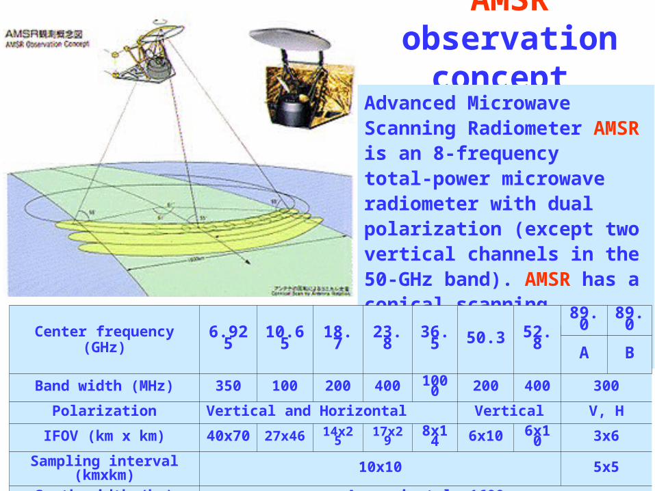
AMSR observation concept

Advanced Microwave Scanning Radiometer AMSR is an 8-frequency total-power microwave radiometer with dual polarization (except two vertical channels in the 50-GHz band). AMSR has a conical scanning geometry. Incidence angle is 55 deg.

Center frequency (GHz) 6.925 10.65 18.7 23.8 36.5 50.3 52.889.0 89.0

A BBand width (MHz) 350 100 200 400 1000 200 400 300

Polarization Vertical and Horizontal Vertical V, H

IFOV (km x km) 40x70 27x46 14x25 17x29 8x14 6x10 6x10 3x6

Sampling interval (kmxkm) 10x10 5x5

Swath width (km) Approximately 1600

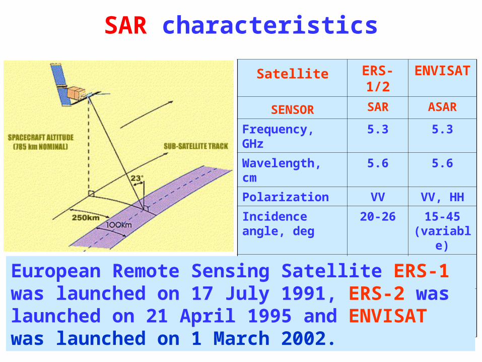
SAR characteristics

Satellite ERS-1/2 ENVISAT

SENSOR SAR ASAR

Frequency, GHz 5.3 5.3

Wavelength, cm 5.6 5.6

Polarization VV VV, HH

Incidence angle, deg

20-26 15-45 (variable)

Swath width, km 100 100-405

Ground resolution , m

25 x 25 25 x 25150x150

European Remote Sensing Satellite ERS-1 was launched on 17 July 1991, ERS-2 was launched on 21 April 1995 and ENVISAT was launched on 1 March 2002.

Envisat ASAR

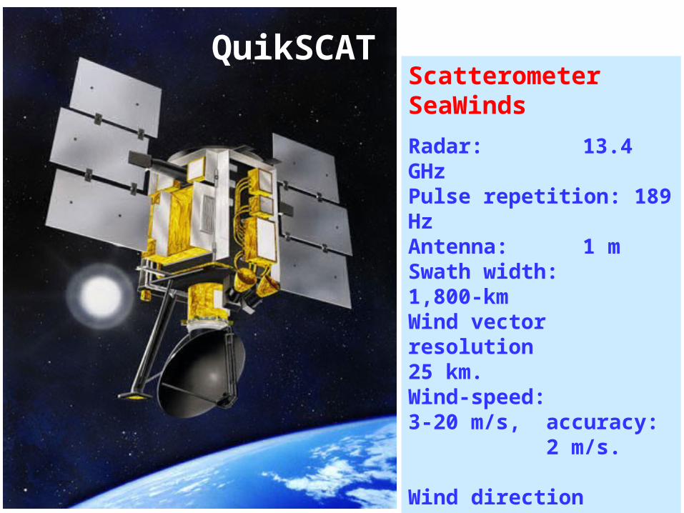
Scatterometer SeaWinds

Radar: 13.4 GHzPulse repetition: 189 Hz Antenna: 1 m Swath width: 1,800-km Wind vector resolution 25 km.Wind-speed: 3-20 m/s, accuracy: 2 m/s. Wind direction accuracy: 20 deg.

Rotating dish produces two spot beams, sweeping in a circular pattern. 90% coverage of Earth's oceans every day.

QuikSCAT

Satellite SAR

Precision (PRI) and quick look (QL) ERS-2 SAR and Envisat ASAR images taken in 2002-2005 are used for the sea ice study in the Okhotsk and Japan Seas. High spatial resolution of a SAR permits to determine the areas of grease ice, pancake ice and transition zone between them. The growth rate of the ice-covered areas can be estimated by comparison of the overlapping SAR images acquired on ascending and descending orbits.

ADEOS-II AMSR and Aqua AMSR-E data, NOAA AVHRR and MODIS images, QuikSCAT-derived wind fields as well as weather maps were used to confirm interpretation of SAR signatures. Several case studies cover the Aniva Bay and the northern, western and eastern Okhotsk Sea are considered.

SAR image location

Map of the Okhotsk Sea

(1) ERS-2 SAR for 24 Jan 2000 at 01:17 UTC (2) Envisat ASAR for 1 Dec 2004 at 11:46 UTC (3) Envisat

ASAR for 9 Dec 2002 at 12:11 UTC (4) Envisat

ASAR for 28 Feb 2003 at 00:02 UTC (5)

Envisat ASAR for 28 Feb 2003 at 11:25 UTC

1

2

5

4

3

Kamchatka

Hokkaido

Sakhalin

Kunashir

Iturup

Urup

Pacific Ocean

Okhotsk Sea

Japan Sea

Aniva Bay. ERS-2 SAR frames

Bathymetric map off the Hokkaido

coast

Red rectangles mark the location of the ERS-2 SAR images acquired on 18 February 1996 at 01:19 UTC (1) and at 12:39 UTC (2) ; 24 January 2000 and 15 March 1999 at 01:17 UTC (3).

1

2

3

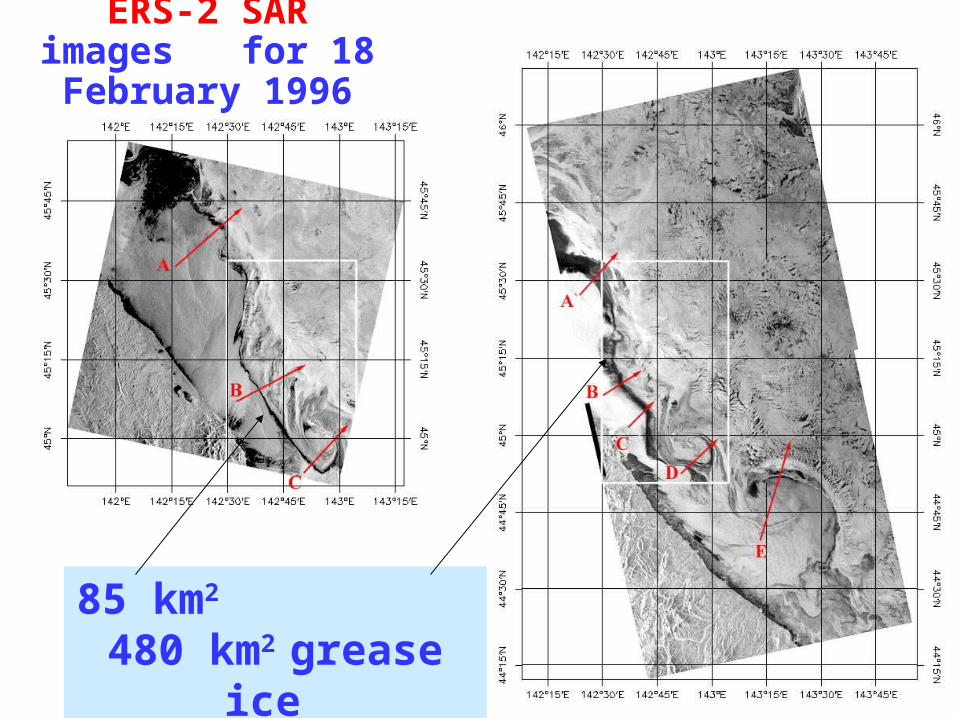
ERS-2 SAR images for 18 February 1996

85 km2 480 km2

grease ice

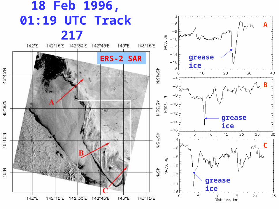
18 Feb 1996, 01:19 UTC Track 217 A

B

C

grease ice

grease ice

grease iceERS-2 SAR

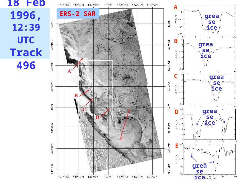
18 Feb 1996,

12:39 UTC Track

496

A

B

C

D

E

grease ice

grease ice

grease ice

grease ice

grease ice

ERS-2 SAR

Ice drift and ice eddies

The change of ice cover off Hokkaido for 11 h 20 min

Ice edge at 01:19 UTC

Ice edge at 12:39 UTC

Grease ice

01:19 UTC 12:39 UTCERS-2 SAR

Envisat ASAR

Fragment of ASAR quick look image with HH-pol at 11:46 UTC (a) and SeaWinds-derived wind field at 10:02 UTC on 1 December 2004 (b).

The ice bands 1 and ice field 2 have negative contrast against the open sea likely due to the presence of the grease ice. Ice fields 3 is in the area where wind speed lower than to the west of it. Their brightness is higher compare to 1 and 2 likely due to the presence of the pancake ice. The narrow dark bands adjacent to the fields 3 are very likely grease ice. The grease ice is clearly seen on the upwind side of ice massive 4. Its area is 16300 km2 and the grease ice area is 1600 km2.

1

2 3

4A B

5

(a) (b) QuikSCAT

ESA 2004

Surface analysis

map of the JMH for

1 Dec 2004 at 12:00

UTC.

Pink rectangle marks the

boundaries of Envisat ASAR image taken on 1 Dec 2004 at 11:46 UTC.

Sakhalin

QuikSCAT SeaWinds.1 Dec 2004, 19.50 UTC

Sakhalin

Envisat ASAR 1 Dec 2004

2

3

ESA 2004

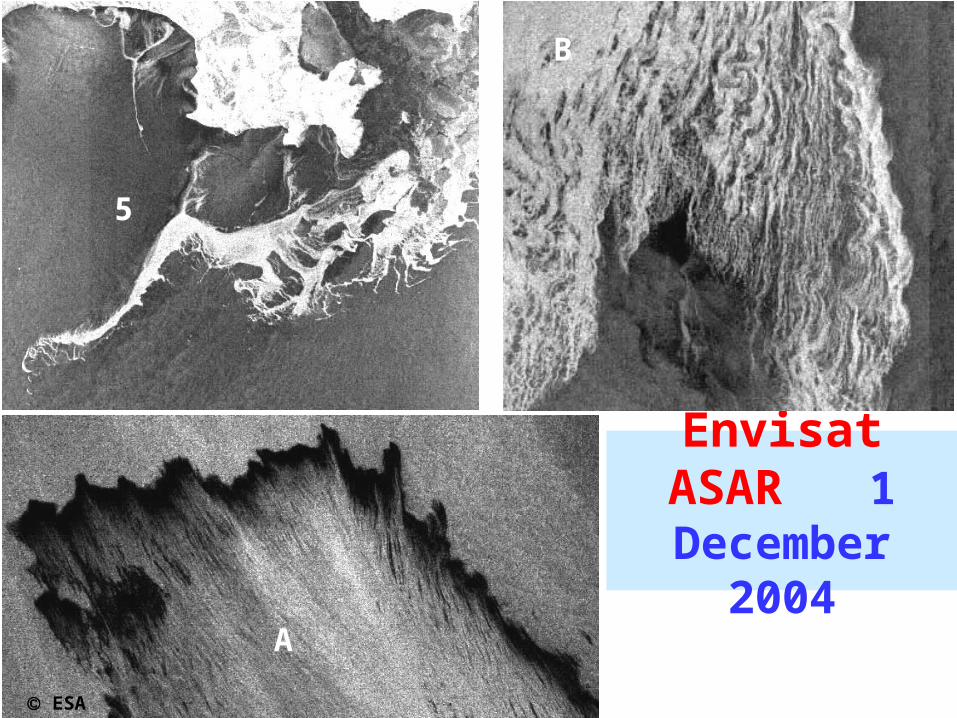
Envisat ASAR 1 December 2004

5

B

A

ESA 2004

Envisat ASAR

1 December

2004 at 11:46

UTC 4

ESA 2004

Western Okhotsk sea(a)

(b)

2

1

© ESA 2002

Envisat ASAR, HH, 12:11 UTCAqua AMSR-E at 15:23 UTC, 36.5 GHz, H-polarization

9 December 2002

Grease ice

3260 km2.

Pancake ice 6470 km2.

Envisat ASAR

Sakhalin

Sakhalin

(1)

(3)

(2)

(2)

NOAA AVHRR9 December 2002

Hokkaido

Kamchatka

Envisat ASAR

Sakhalin

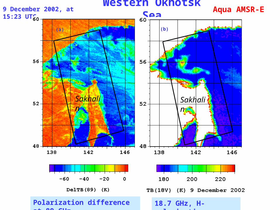
Western Okhotsk Sea

Polarization difference at 89 GHz 18.7 GHz, H-polarization

9 December 2002, at 15:23 UTC

1

22

(a) (b)

Aqua AMSR-E

Sakhalin Sakhalin

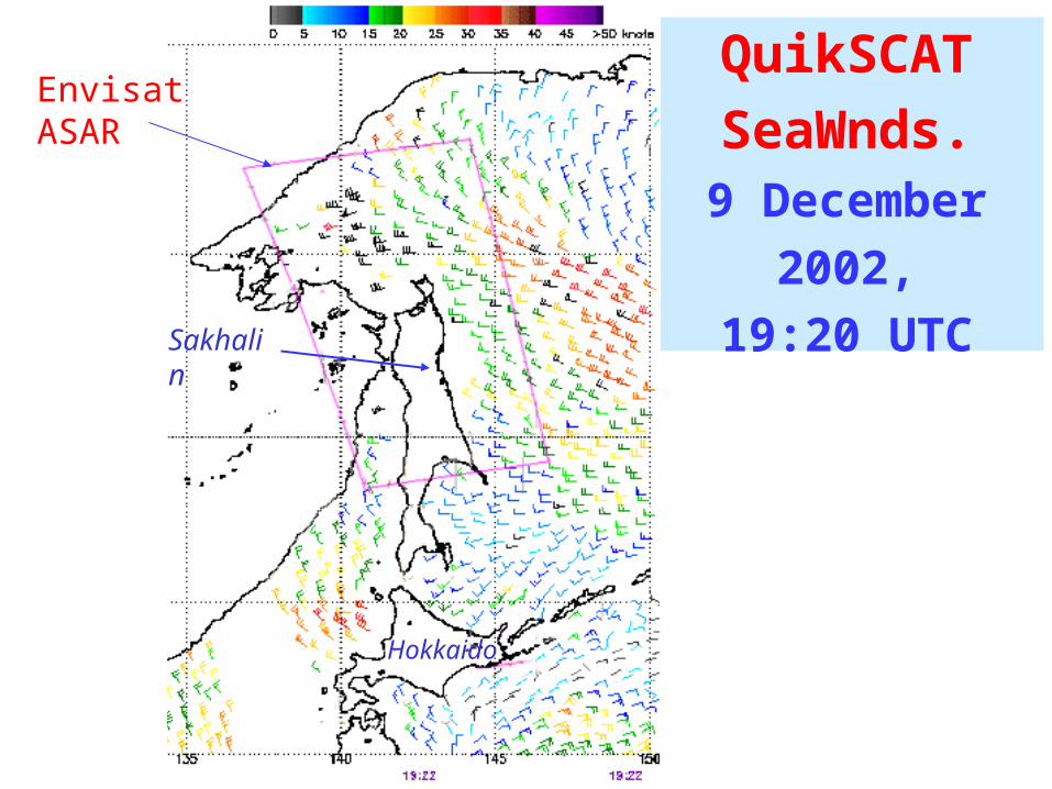
QuikSCAT

SeaWnds.9 December 2002,

19:20 UTC

Envisat ASAR

Sakhalin

Hokkaido

Envisat ASAR,HH,

9 December 2002,

12:11 UTCSakhalin

ESA 2002

Envisat ASAR

HH 9 Dec 2002 12:11 UTC

Sakhalin ESA 2002

NRCS profiles

A

B C

water

greaseice

pancakeice

hammock

gray-whiteIce?

polynya

water

greaseice

greaseice

pancakeice pancake

ice

hammock hammock

greaseice

Envisat ASAR, 9 Dec 2002, 12: 11 UTC

Patches of sea ice in the open sea

ESA 2002

Envisat ASAR

30 January 2005

31 January 2005

Sak

halin

ESA 2005 ESA 2005

Envisat ASAR,

11:31 UTC

31 January 2005

QuikSCAT SeaWinds 8:48 UTC

Sak

halin

MODIS 14 January

2005

Envisat ASAR images

taken on 14 January

2005at 00:41 and

at 12:04 UTC

Sakhalin Sakhalin

ESA 2005 ESA 2005

Envisat ASAR images taken at 00:41 UTC and at 12:04 UTC on 14 January 2005

Surface analysis map of the JMH for 28 February 2003, 00:00 UTC

Red rectangles mark the boundaries of Envisat ASAR images taken on 28 Feb 2003

at 00:00 UTC (1) and at 11:25 UTC (2)

(2)

(1)

Kam

chatk

a

Eastern Okhotsk Sea

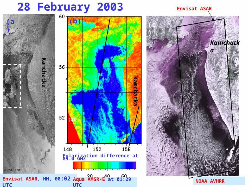
28 February 2003

© ESA 2003

Kamchatka

(d)

(c)(a) (b)

4

2

1

4

3

1

Envisat ASAR, HH, 00:02 UTC

Envisat ASAR

NOAA AVHRR

Polarization difference at 89.0 GHz

Aqua AMSR-E at 01:29 UTC

Kam

chatk

a

Kam

chatk

a

28 February 2003

1

2

2

(e) (f)

Envisat ASAR, HH, 11:25 UTC

Aqua AMSR-E. 15:29 UTC TB(36V)

QuikSCAT SeaWinds-derived wind field at 08:08 UTC

Kamchatka

Kam

chatk

a

Kam

chatk

a

© ESA 2003

Envisat ASAR28 Feb

2003 at 00:02 and at 11:25

UTC

© ESA 2003 © ESA 2003

ConclusionsThis study has demonstrated the utility of a multiscale multisensor approach for the sea ice study in the Okhotsk Sea. Data from satellite SAR, microwave scanning radiometer, scatterometer, AVHRR and MODIS were used for several case studies in different regions of the Sea. The sensors were chosen for their temporal simultaneity of measurement collection.

The primary attention was given to the satellite SAR due to the high spatial resolution capability of the instruments. SAR can provide precise data on the location and type of ice boundary, concentration and the presence or absence of polynyas and leads. Interpretation of SAR images is not straightforward due to the ambiguities associated with SAR backscatter from sea ice features that vary by season and geographic region.

Application of AMSR, AMSR-E, SeaWinds scatterometer and MODIS visible/ infrared observations decreases the ambiguities in the interpretation of SAR data.

Acknowledgments This study was carried out within•the cooperation between National Space Development Agency JAXA (Japan) and V.I. Il’ichev Pacific Oceanological Institute, Far Eastern Branch of the Russian Academy of Sciences (Russia) in the ADEOS-II Research Activity

(PROJECTS A2ARF006 and AD2M-3RA-UF002) as well as within •ESA ERS project AO3-401: “Mesoscale oceanic and atmospheric phenomena in the coastal area of the Japan and Okhotsk seas: Study with ERS SAR and research vessels” and •ESA Envisat project AO-ID-391: “Study of the interaction of oceanic and atmospheric processes in the Japan Sea and the Southern Okhotsk Sea”.

This work is partially sponsored by a grant for a project: “Investigation of ocean-atmosphere system with passive and active microwave sensing from new generation satellites” from Far Eastern Branch of the Russian Academy of Sciences.