Thanks to the authors of the

Supercomputing 2012 Tutorial,

nominally:

Kenneth Moreland W. Alan Scott Nathan Fabian

Sandia National Laboratories

Utkarsh Ayachit Robert Maynard

Kitware, Inc.

Sandia is a multiprogram laboratory operated by Sandia Corporation, a Lockheed Martin Company,

under contract DE-AC04-94AL85000.

Introduction to ParaView

Seán Óg Delaney,

Irish Centre for High End Computing

Visualisation Training Day @ EPCC

Prace Summer of HPC, July 2013

Outline

ParaView What is it? Why use it? Who uses it?

GUI intro, Graphics Pipeline, File Formats

Filters

Views and Multi-View

Streamlines, Line Plots

Time Dependent Data

Selections

Python traces

Advanced Topics Paraview at scale

Install ParaView 3.98.1 (or 4.0.0).

http://www.paraview.org Download

Get example material. http://www.paraview.org/Wiki/The_ParaView_Tutorial

Data also available on tutorial handout USB stick.

Help / Information

Online Help F1

http://paraview.org/Wiki/ParaView/Users_Guide/Table_Of_Contents

The ParaView web page

www.paraview.org

ParaView mailing list

paraview@paraview.org

Why ParaView?

Open-source

Multi-platform

Easy (open, flexible, and intuitive UI).

Scalable (does large visualisations on clusters)

An extensible, modular architecture based on open standards.

A flexible BSD 3 Clause license

Commercial maintenance and support.

Renato N. Elias, NACAD/COPPE/UFRJ, Rio de Janerio, Brazil Swiss National Supercomputing Centre

Jerry Clarke, US Army Research Laboratory

Current ParaView Usage

Used by academic, government, and commercial institutions worldwide.

Downloaded ~100K times per year.

HPCwire HPCwire Choice 2010 Awards for Best Visualization Product or Technology.

ParaView Application Architecture

MPI OpenGL IceT Etc.

VTK

ParaView Server

ParaView Client pvpython Custom App

UI (Qt Widgets, Python Wrappings)

Data Types

Uniform Rectilinear

(vtkImageData)

Non-Uniform Rectilinear

(vtkRectilinearData)

Curvilinear

(vtkStructuredData)

Polygonal

(vtkPolyData)

Unstructured Grid

(vtkUnstructuredGrid)

Multi-block Hierarchical Adaptive

Mesh Refinement

(AMR)

Hierarchical Uniform

AMR

Octree

Graphical User Interface (GUI)

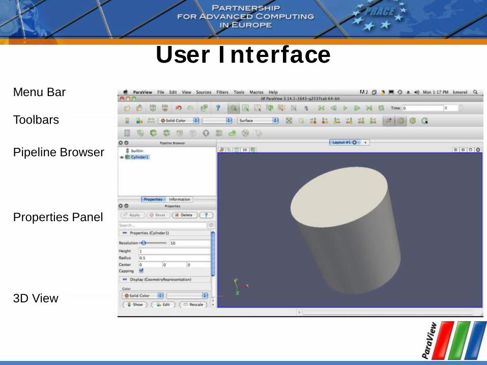
User Interface

Menu Bar

Toolbars

Pipeline Browser

Properties Panel

3D View

Getting Back GUI Components

Creating a Cylinder Source

1. menu and select Cylinder.

2. Click the Apply button to accept the default parameters.

Simple Camera Manipulation

Drag left, middle, right rotate, pan, zoom.

Also use Shift, Ctrl, Alt modifiers.

Creating a Cylinder Source

1. Go to the Sources menu and select Cylinder.

2. Click the Apply button to accept the default parameters.

3. Change the Height parameter to 0.1.

4. Click the Apply button again.

Creating a Cylinder Source

5. Look / Scroll down to the Display properties.

6. Click the Edit button under Color.

7. Change the color.

Creating a Cylinder Source

8. Click on the button at the top of the properties panel.

9. Increase the Resolution parameter.

10. Click the Apply button again.

11. Click again to hide advanced properties.

Pipeline Object Controls

Undo Redo

Redo Undo

Camera

Redo

Camera

Undo

Render View Options

Alternatively, go to Edit -> View Settings...

@ top of layout window

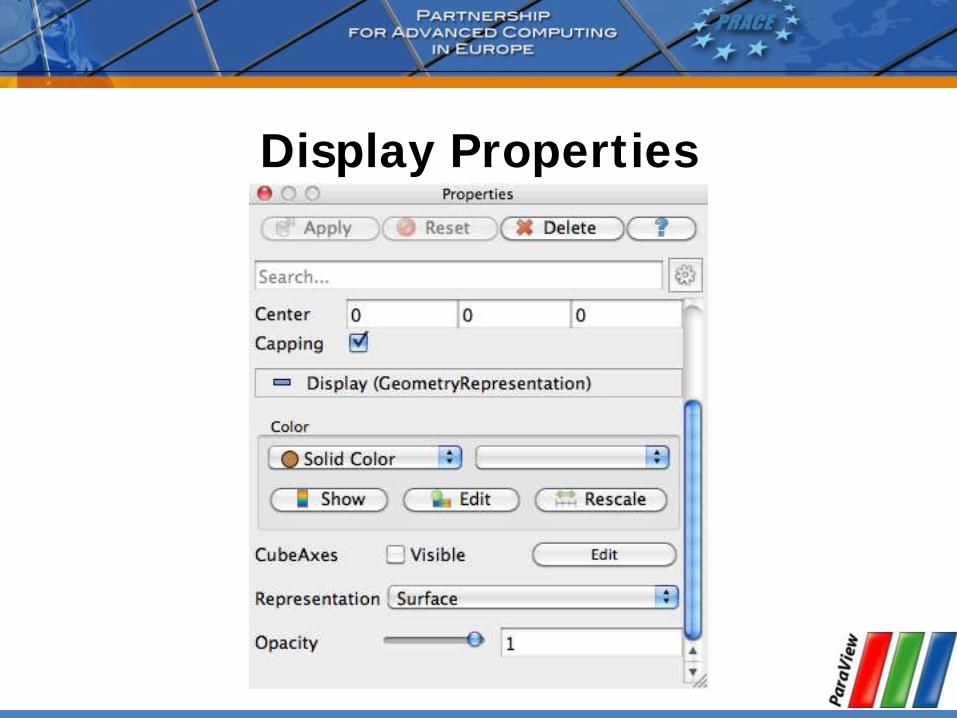
Display Properties

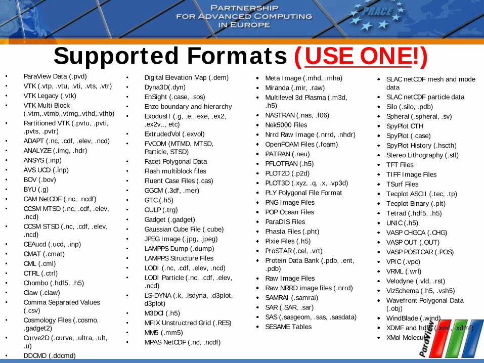
Supported Formats (USE ONE!) ParaView Data (.pvd)

VTK (.vtp, .vtu, .vti, .vts, .vtr)

VTK Legacy (.vtk)

VTK Multi Block (.vtm,.vtmb,.vtmg,.vthd,.vthb)

Partitioned VTK (.pvtu, .pvti, .pvts, .pvtr)

ADAPT (.nc, .cdf, .elev, .ncd)

ANALYZE (.img, .hdr)

ANSYS (.inp)

AVS UCD (.inp)

BOV (.bov)

BYU (.g)

CAM NetCDF (.nc, .ncdf)

CCSM MTSD (.nc, .cdf, .elev, .ncd)

CCSM STSD (.nc, .cdf, .elev, .ncd)

CEAucd (.ucd, .inp)

CMAT (.cmat)

CML (.cml)

CTRL (.ctrl)

Chombo (.hdf5, .h5)

Claw (.claw)

Comma Separated Values (.csv)

Cosmology Files (.cosmo, .gadget2)

Curve2D (.curve, .ultra, .ult, .u)

DDCMD (.ddcmd)

Digital Elevation Map (.dem)

Dyna3D(.dyn)

EnSight (.case, .sos)

Enzo boundary and hierarchy

ExodusII (.g, .e, .exe, .ex2, .ex2v.., etc)

ExtrudedVol (.exvol)

FVCOM (MTMD, MTSD, Particle, STSD)

Facet Polygonal Data

Flash multiblock files

Fluent Case Files (.cas)

GGCM (.3df, .mer)

GTC (.h5)

GULP (.trg)

Gadget (.gadget)

Gaussian Cube File (.cube)

JPEG Image (.jpg, .jpeg)

LAMPPS Dump (.dump)

LAMPPS Structure Files

LODI (.nc, .cdf, .elev, .ncd)

LODI Particle (.nc, .cdf, .elev, .ncd)

LS-DYNA (.k, .lsdyna, .d3plot, d3plot)

M3DCl (.h5)

MFIX Unstructred Grid (.RES)

MM5 (.mm5)

MPAS NetCDF (.nc, .ncdf)

Meta Image (.mhd, .mha)

Miranda (.mir, .raw)

Multilevel 3d Plasma (.m3d, .h5)

NASTRAN (.nas, .f06)

Nek5000 Files

Nrrd Raw Image (.nrrd, .nhdr)

OpenFOAM Files (.foam)

PATRAN (.neu)

PFLOTRAN (.h5)

PLOT2D (.p2d)

PLOT3D (.xyz, .q, .x, .vp3d)

PLY Polygonal File Format

PNG Image Files

POP Ocean Files

ParaDIS Files

Phasta Files (.pht)

Pixie Files (.h5)

ProSTAR (.cel, .vrt)

Protein Data Bank (.pdb, .ent, .pdb)

Raw Image Files

Raw NRRD image files (.nrrd)

SAMRAI (.samrai)

SAR (.SAR, .sar)

SAS (.sasgeom, .sas, .sasdata)

SESAME Tables

SLAC netCDF mesh and mode data

SLAC netCDF particle data

Silo (.silo, .pdb)

Spheral (.spheral, .sv)

SpyPlot CTH

SpyPlot (.case)

SpyPlot History (.hscth)

Stereo Lithography (.stl)

TFT Files

TIFF Image Files

TSurf Files

Tecplot ASCII (.tec, .tp)

Tecplot Binary (.plt)

Tetrad (.hdf5, .h5)

UNIC (.h5)

VASP CHGCA (.CHG)

VASP OUT (.OUT)

VASP POSTCAR (.POS)

VPIC (.vpc)

VRML (.wrl)

Velodyne (.vld, .rst)

VizSchema (.h5, .vsh5)

Wavefront Polygonal Data (.obj)

WindBlade (.wind)

XDMF and hdf5 (.xmf, .xdmf)

XMol Molecule

Load disk_out_ref.ex2

1. Open the file disk_out_ref.ex2.

2. Load all data variables.

3. Click

Data Representation

Toggle Color

Legend

Mapped

Variable

Representation

Vector

Component

Edit

Colors

Reset Scalar

Range

Geometry Representations

Points Wireframe Surface Surface

with Edges

Volume

Introduction to Filters

Common Filters

Calculator

Contour

Clip

Slice

Threshold

Extract Subset

Glyph

Stream Tracer

Warp (vector)

Group Datasets

Extract Level

Filters Menu

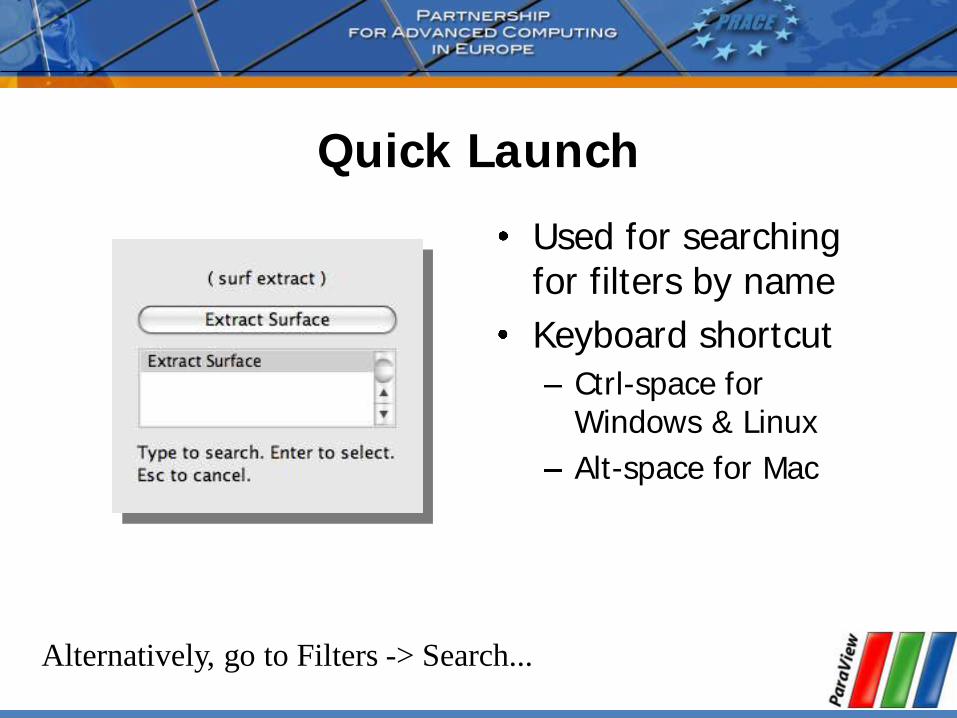
Quick Launch

Used for searching for filters by name

Keyboard shortcut

Ctrl-space for Windows & Linux

Alt-space for Mac

Alternatively, go to Filters -> Search...

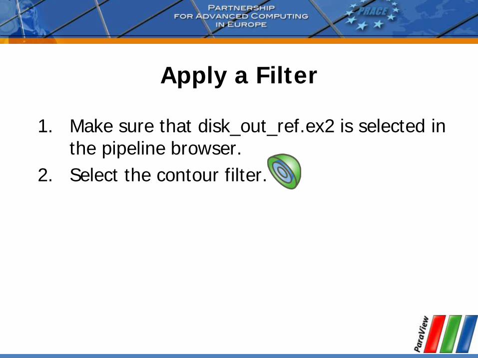
Apply a Filter

1. Make sure that disk_out_ref.ex2 is selected in the pipeline browser.

2. Select the contour filter.

Apply a Filter

3. Change parameters to create an isosurface at Temp = 400K.

Change to Temp

Change to 400

Apply a Filter

1. Make sure that disk_out_ref.ex2 is selected in the pipeline browser.

2. Select the contour filter.

3. Change parameters to create an isosurface at Temp = 400K.

4.

Create a Cutaway Surface

1. Select disk_out_ref.ex2 in the pipeline browser.

2. From the quick launch, select Extract Surface.

3.

Create a Cutaway Surface

1. Select disk_out_ref.ex2 in the pipeline browser.

2. From the quick launch, select Extract Surface.

3.

4. Create a clip filter.

5. Uncheck Show Plane.

6.

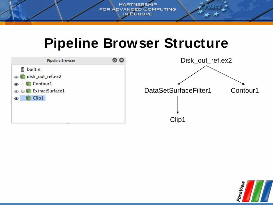
Pipeline Browser Structure Disk_out_ref.ex2

Contour1 DataSetSurfaceFilter1

Clip1

Reset ParaView

Views and Multiview

Multiview

Multiview

1. Open disk_out_ref.ex2. Load all variables.

2. Add clip filter.

3. Uncheck Show Plane.

4.

5. Color surface by Pres.

Multiview

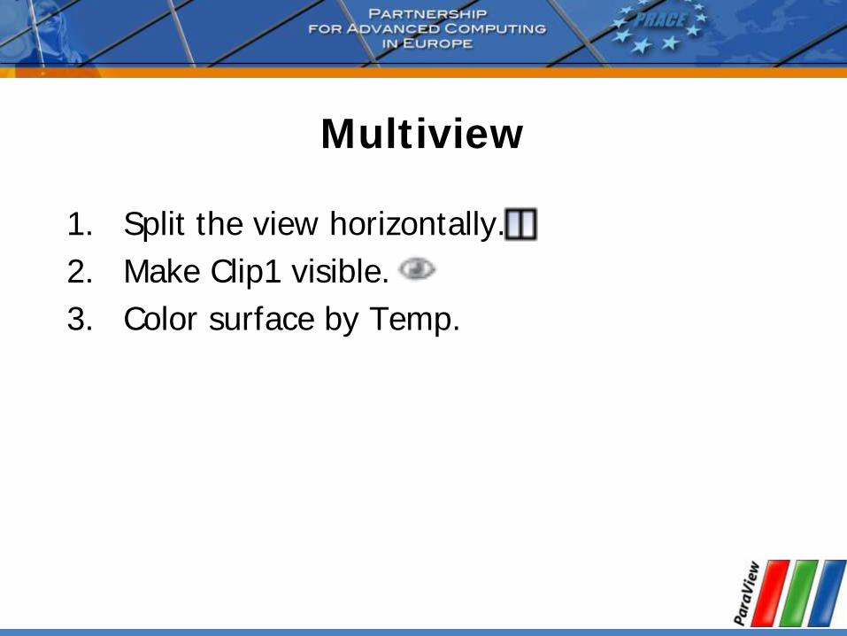
1. Split the view horizontally.

2. Make Clip1 visible.

3. Color surface by Temp.

Multiview

1. Split the view horizontally.

2. Make Clip1 visible.

3. Color surface by Temp.

4. Right-

5. Click other view.

Multiview

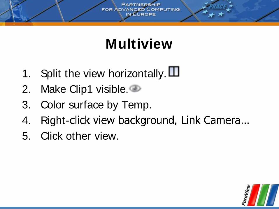
1. Split the view horizontally.

2. Make Clip1 visible.

3. Color surface by Temp.

4. Right-

5. Click other view.

6. Click

Modifying Views

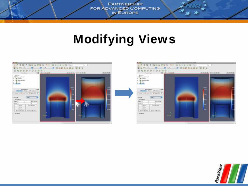
Modifying Views

Reset ParaView

Streamlines

1. Open disk_out_ref.ex2. Load all variables.

2. Add stream tracer.

3.

Streamlines

1. Open disk_out_ref.ex2. Load all variables.

2. Add stream tracer.

3.

4. From the quick launch, select Tube

5.

Getting Fancy

1. Select StreamTracer1.

2. Add glyph filter.

3. Change Vectors to V.

4. Change Glyph Type to Cone.

5.

Getting Answers

Where is the air moving the fastest? Near the disk or away from it? At the center of the disk or near its edges?

Which way is the plate spinning?

At the surface of the disk, is air moving toward the center or away from it?

Reset ParaView

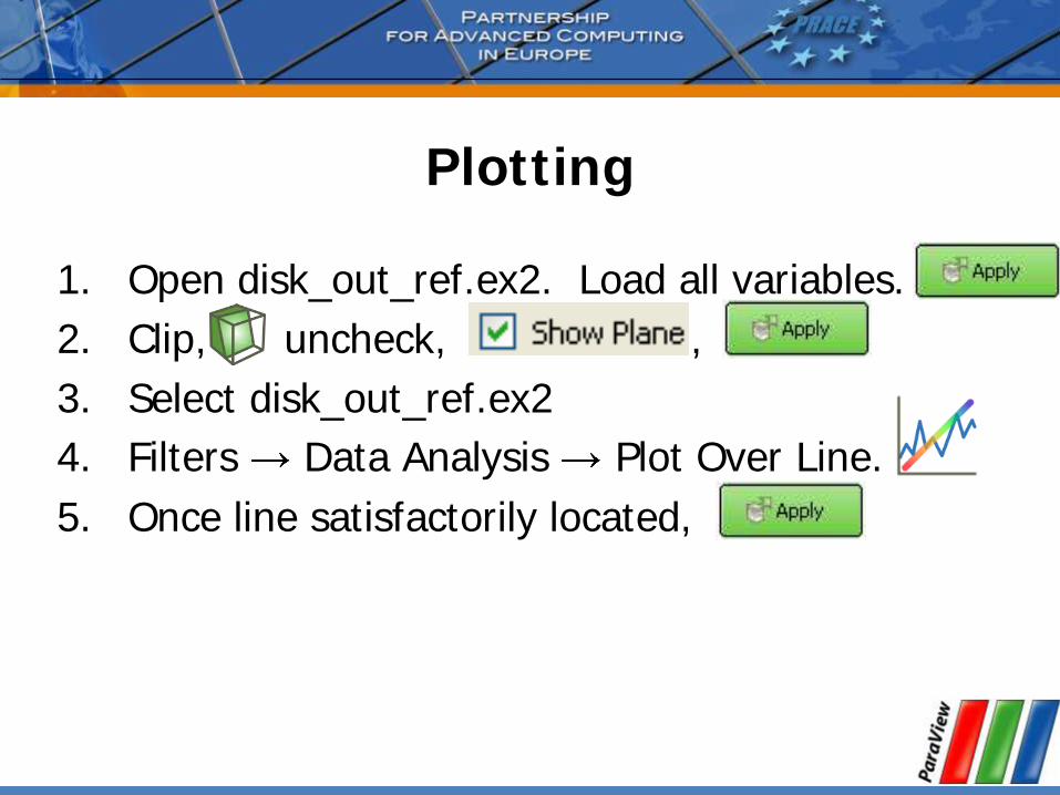
Plotting

1. Open disk_out_ref.ex2. Load all variables.

2. Clip, uncheck, ,

3. Select disk_out_ref.ex2

4. Filters Data Analysis Plot Over Line.

3D Widgets

Plotting

1. Open disk_out_ref.ex2. Load all variables.

2. Clip, uncheck, ,

3. Select disk_out_ref.ex2

4. Filters Data Analysis Plot Over Line.

5. Once line satisfactorily located,

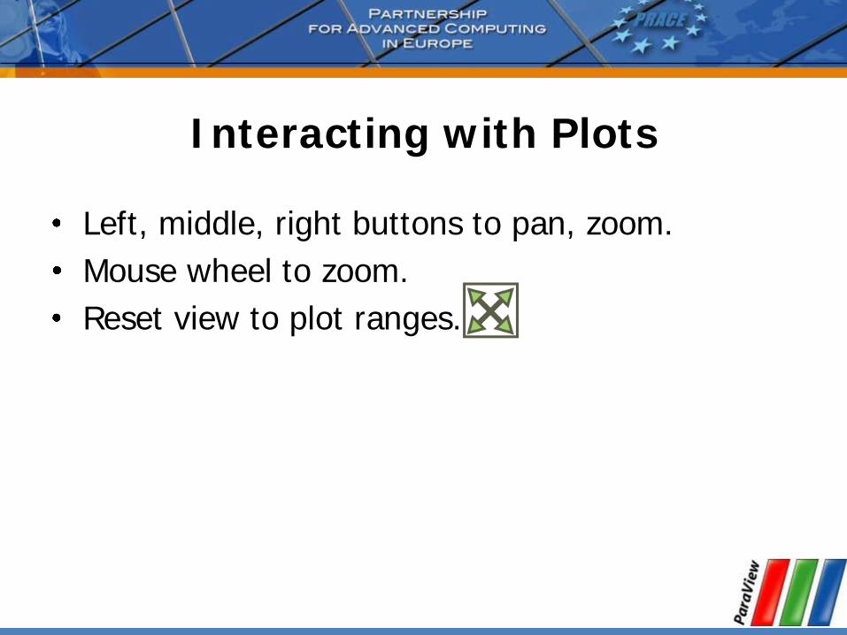
Interacting with Plots

Left, middle, right buttons to pan, zoom.

Mouse wheel to zoom.

Reset view to plot ranges.

Plots are Views Move them like Views.

Save screenshots.

Adjusting Plots

1. In Display tab, turn off all variables except Temp and Pres.

2. Select Pres in the Display tab.

3. Change Chart Axis to Bottom Right.

4. Verify the relationship between temperature and pressure.

Reset ParaView

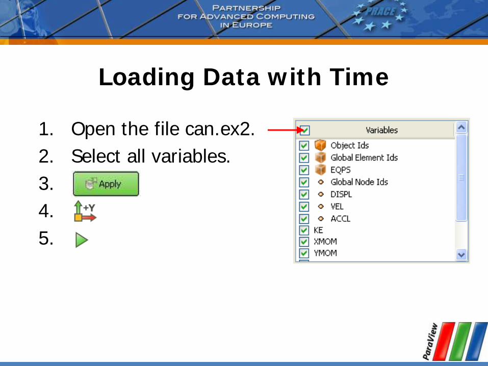
Loading Data with Time

1. Open the file can.ex2.

2. Select all variables.

3.

4.

5.

Animation Toolbar

First

Frame

Previous

Frame Play

Next

Frame

Last

Frame

Loop

Animation

Current

Time

Current

Time Step

Data Range Workarounds

Open color scale editor dialog

Rescale to Temporal Range

Save Screenshot/Animation

1. Choose File

2. Complete the subsequent dialogs to save an image.

3. Chose File

4. Complete the subsequent dialogs to save a movie.

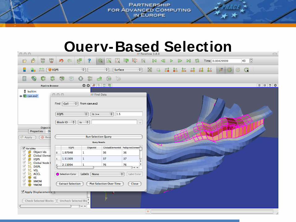
Query-Based Selection

1. Open can.ex2. All variables.

2. Go to last time step.

3. Edit Find Data.

4. Top combo box: find Cells.

5. Next row: EQPS, is >=, and 1.5.

6. Click Run Selection Query.

Query-Based Selection

Brush Selection

Surface Cell Selection (shortcut: s)

Surface Point Selection

Through Cell Selection

Through Point Selection

Block Selection (shortcut: b)

Selection Inspector

Create new selection

Active selection

properties

Selected cells ids

Selection type

Selection display

Properties/Labeling

Spreadsheet View

1. Split the view

2. In new view, click Spreadsheet View.

Spreadsheet View

Show only

selected items

Select block

to inspect

What is

shown in

the view

Attribute shown

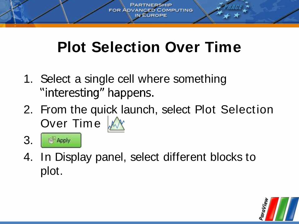
Plot Selection Over Time

1. Select a single cell where something

2. From the quick launch, select Plot Selection Over Time

3.

4. In Display panel, select different blocks to plot.

Reset ParaView

Extracting a Selection

1. Open can.ex2. Load all variables.

2. Turn off cell labels.

3. Perform a sizeable selection.

4. From the quick launch, select Extract Selection

5.

Python Trace Demo

Visualizing Large Models

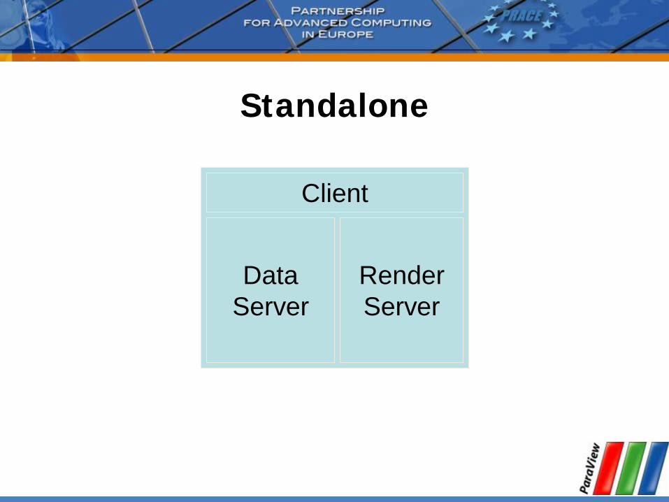
Standalone

Client

Data

Server

Render

Server

Client-Server

Client Data

Server

Render

Server

Client-Render Server-Data Server

Client Data

Server

Render

Server

Requirements for Installing ParaView Server

C++

CMake (www.cmake.org)

MPI

OpenGL (or Mesa3D www.mesa3d.org)

Qt 4.6 (optional)

Python (optional) http://www.paraview.org/Wiki/Setting_up_a_ParaView_Server#Compiling

Connecting to a ParaView Server

http://www.paraview.org/Wiki/Setting_up_a_ParaView_Server#Running_the_Server

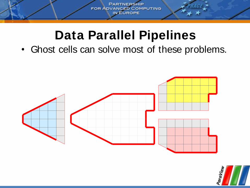
Data Parallel Pipelines Ghost cells can solve most of these problems.

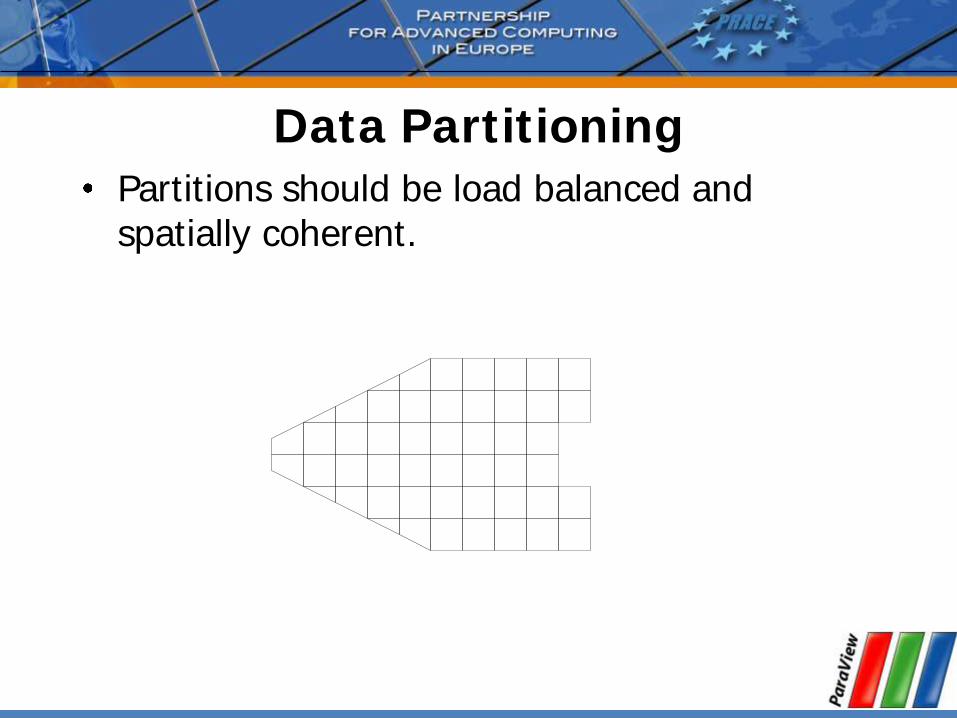
Data Partitioning

Partitions should be load balanced and spatially coherent.

Load Balancing/Ghost Cells

Automatic for Structured Meshes.

Partitioning/ghost cells for unstructured is

Use the D3 filter for unstructured

(Filters Alphabetical D3)

Job Size Rules of Thumb

Structured Data

Try for max 20 M cell/processor.

Shoot for 5 10 M cell/processor.

Unstructured Data

Try for max 1 M cell/processor.

Shoot for 250 500 K cell/processor.

Avoiding Data Explosion

Pipeline may cause data to be copied, created, converted.

This advice only for dealing with very large amounts of data.

Remaining available memory is low.

Topology Changing, No Reduction

Append Datasets

Append Geometry

Clean

Clean to Grid

Connectivity

D3

Delaunay 2D/3D

Extract Edges

Linear Extrusion

Loop Subdivision

Reflect

Rotational Extrusion

Shrink

Smooth

Subdivide

Tessellate

Tetrahedralize

Triangle Strips

Triangulate

Topology Changing, Moderate Reduction

Clip

Decimate

Extract Cells by Region

Extract Selection

Quadric Clustering

Threshold

Similar: Extract Subset

Topology Changing, Dimension Reduction

Cell Centers

Contour

Extract CTH Fragments

Extract CTH Parts

Extract Surface

Feature Edges

Mask Points

Outline (curvilinear)

Slice

Stream Tracer

Adds Field Data

Block Scalars

Calculator

Cell Data to Point Data

Compute Derivatives

Curvature

Elevation

Generate Ids

Gen. Surface Normals

Gradient

Level Scalars

Median

Mesh Quality

Octree Depth Limit

Octree Depth Scalars

Point Data to Cell Data

Process Id Scalars

Random Vectors

Resample with dataset

Surface Flow

Surface Vectors

Transform

Warp (scalar)

Warp (vector)

Total Shallow Copy or Output Independent of Input

Annotate Time

Append Attributes

Extract Block

Extract Datasets

Extract Level

Glyph

Group Datasets

Histogram

Integrate Variables

Normal Glyphs

Outline

Outline Corners

Plot Global Variables Over Time

Plot Over Line

Plot Selection Over Time

Probe Location

Temporal Shift Scale

Temporal Snap-to-Time-Steps

Temporal Statistics

Culling Data

Reduce dimensionality early.

Prefer data reduction over extraction.

Slice instead of Clip.

Contour instead of Threshold.

Only extract when reducing an order of magnitude or more.

Can still run into trouble.

Culling Data

Experiment with subsampled data.

Extract Subset

Use caution.

Subsampled data may be lacking.

Use full data to draw final conclusions.

Rendering Modes

Still Render

Full detail render.

Interactive Render

Sacrifices detail for speed.

Provides quick rendering rate.

Used when interacting with 3D view.

Level of Detail (LOD) Geometric decimation

Used only with Interactive Render

Original Data Divisions: 50x50x50 Divisions: 10x10x10

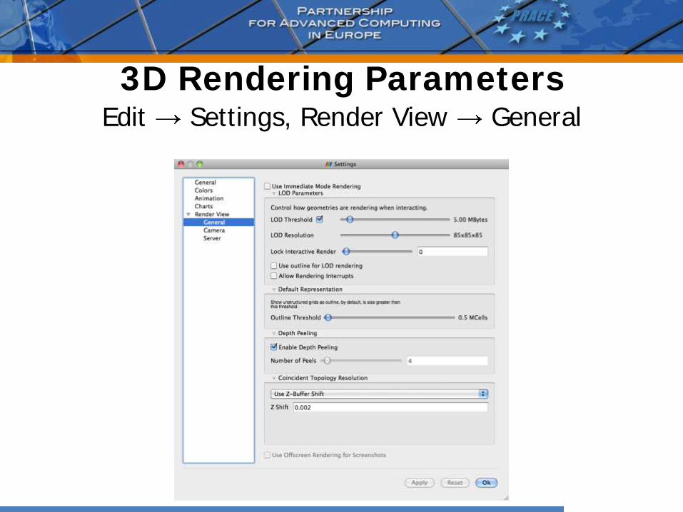
3D Rendering Parameters Edit Settings, Render View General

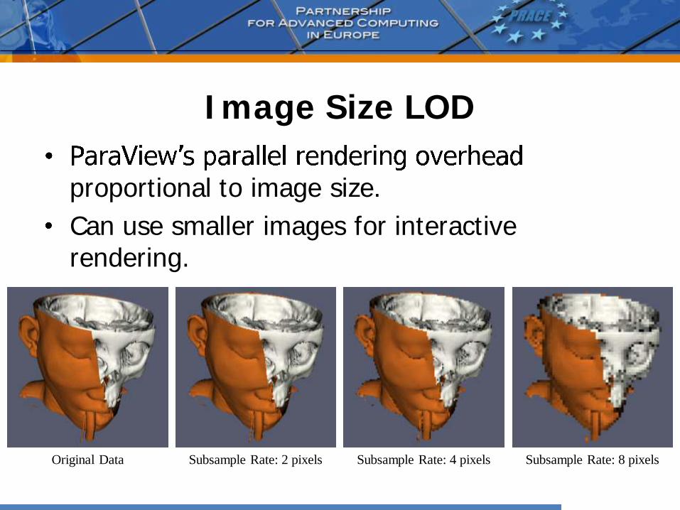
Image Size LOD

proportional to image size.

Can use smaller images for interactive rendering.

Original Data Subsample Rate: 2 pixels Subsample Rate: 4 pixels Subsample Rate: 8 pixels

Parallel Rendering Parameters Edit Settings, Render View Server

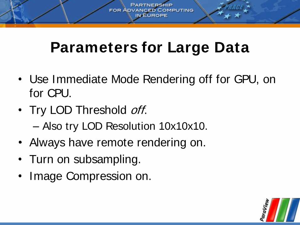
Parameters for Large Data

Use Immediate Mode Rendering off for GPU, on for CPU.

Try LOD Threshold off.

Also try LOD Resolution 10x10x10.

Always have remote rendering on.

Turn on subsampling.

Image Compression on.

Parameters for Low Bandwidth

Try larger subsampling rates.

Try Zlib compression and fewer bits.

Parameters for High Latency

Turn up Remote Render Threshold.

Turn on Use outline for LOD rendering if necessary.

Play with the LOD Threshold and LOD Resolution to control geometry sent to client.

Try turning on Lock Interactive Render.

Further Reading

Amy Henderson Squillacote. The ParaView Guide. Kitware, Inc., 2006.

http://www.paraview.org/Wiki/ParaView

http://www.paraview.org/Wiki/Setting_up_a_ParaView_Server