Texture Mapping & Shaders - MIT OpenCourseWare · PDF fileTexture Mapping & Shaders ... the...

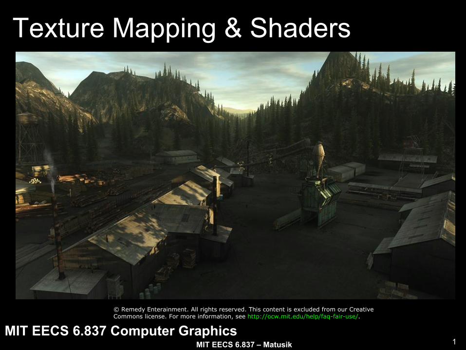
MIT EECS 6.837 Computer Graphics

1 MIT EECS 6.837 – Matusik

Texture Mapping & Shaders

© Remedy Enterainment. All rights reserved. This content is excluded from our CreativeCommons license. For more information, see http://ocw.mit.edu/help/faq-fair-use/.

http://ocw.mit.edu/help/faq-fair-use/

2

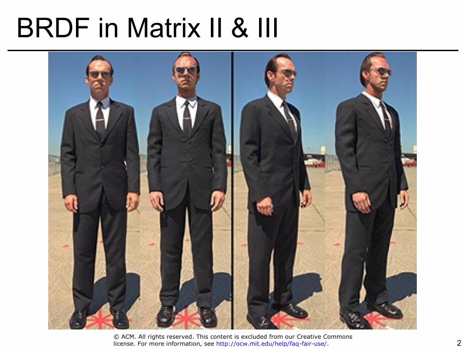
BRDF in Matrix II & III

© ACM. All rights reserved. This content is excluded from our Creative Commonslicense. For more information, see http://ocw.mit.edu/help/faq-fair-use/.


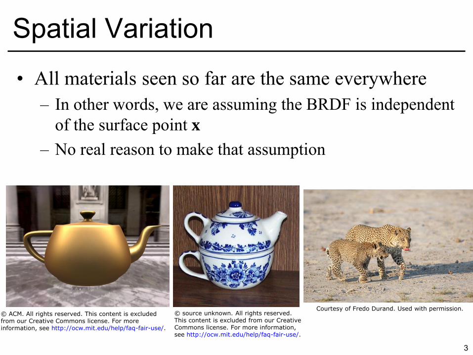
• All materials seen so far are the same everywhere – In other words, we are assuming the BRDF is independent

of the surface point x

– No real reason to make that assumption

3

Spatial Variation

© ACM. All rights reserved. This content is excludedfrom our Creative Commons license. For moreinformation, see http://ocw.mit.edu/help/faq-fair-use/.

Courtesy of Fredo Durand. Used with permission.© source unknown. All rights reserved.This content is excluded from our CreativeCommons license. For more information,see http://ocw.mit.edu/help/faq-fair-use/.



• We will allow BRDF parameters to vary over space – This will give us much more complex surface appearance – e.g. diffuse color kd vary with x – Other parameters/info can vary too: ks, exponent, normal

4

Spatial Variation

© ACM. All rights reserved. This content is excludedfrom our Creative Commons license. For moreinformation, see http://ocw.mit.edu/help/faq-fair-use/.

Courtesy of Fredo Durand. Used with permission.© source unknown. All rights reserved.This content is excluded from our CreativeCommons license. For more information,see http://ocw.mit.edu/help/faq-fair-use/.



• From data : texture mapping – read color and other information

from 2D images

• Procedural : shader – write little programs that compute

color/info as a function of location

5

Two Approaches


© Ken Perlin. All rights reserved. This content is excluded from our Creative Commonslicense. For more information, see http://ocw.mit.edu/help/faq-fair-use/.



6

Effect of Textures

Courtesy of Jeremy Birn.

7

Texture Mapping

Image of a cartoon of a man applying wall paper has been removed due to copyright restrictions.

8

Texture Mapping 3D model Texture mapped model

Image: Praun et al.

?

© ACM. All rights reserved. This content is excluded from our Creative Commonslicense. For more information, see http://ocw.mit.edu/help/faq-fair-use/.© Oscar Meruvia-Pastor, Daniel Rypl. All rights reserved. This

content is excluded from our Creative Commons license. Formore information, see http://ocw.mit.edu/help/faq-fair-use/.



http://doi.acm.org/10.1145/566654.566590

9

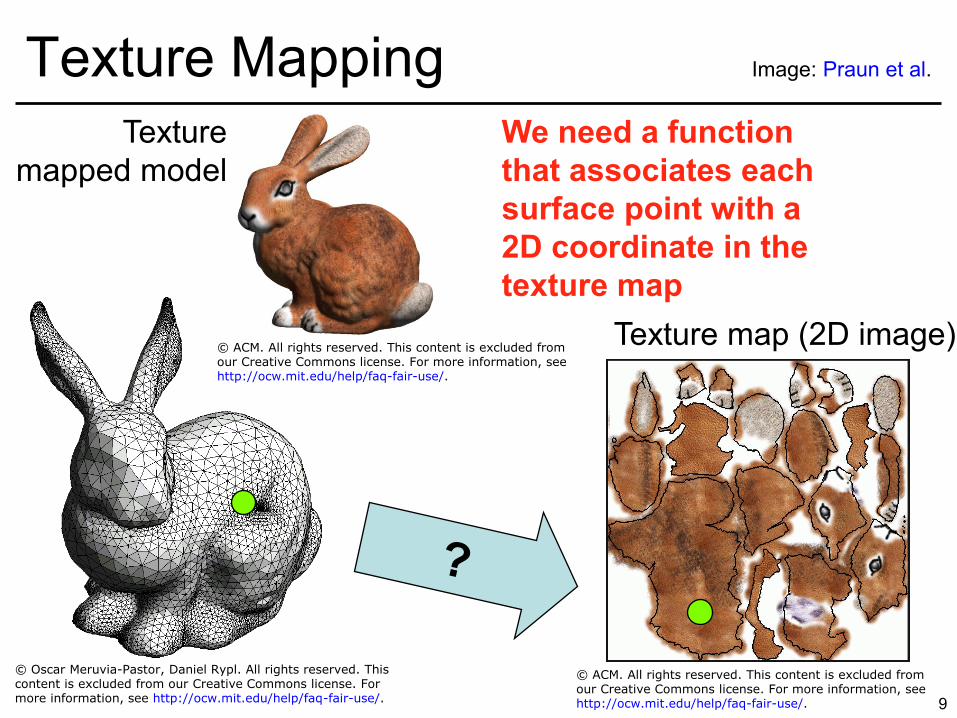
Texture Mapping Texture

mapped model

Image: Praun et al.

Texture map (2D image)

We need a function

that associates each

surface point with a

2D coordinate in the

texture map

© ACM. All rights reserved. This content is excluded fromour Creative Commons license. For more information, seehttp://ocw.mit.edu/help/faq-fair-use/.


© Oscar Meruvia-Pastor, Daniel Rypl. All rights reserved. Thiscontent is excluded from our Creative Commons license. Formore information, see http://ocw.mit.edu/help/faq-fair-use/.




http://doi.acm.org/10.1145/566654.566590

10

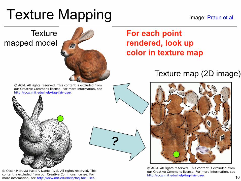
Texture Mapping Texture

mapped model

Image: Praun et al.

Texture map (2D image)

For each point

rendered, look up

color in texture map



© Oscar Meruvia-Pastor, Daniel Rypl. All rights reserved. Thiscontent is excluded from our Creative Commons license. Formore information, see http://ocw.mit.edu/help/faq-fair-use/.




http://doi.acm.org/10.1145/566654.566590

• Each vertex P stores 2D (u, v) “texture coordinates” – UVs determine the 2D location in the texture for the vertex – We will see how to specify them later

• Then we interpolate using barycentrics

11

UV Coordinates

(u0, v0)

(u1, v1) (u2, v2) u

v (αu0+βu1+γu2, αv0+βv1+γv2)

• Each vertex P stores 2D (u, v) “texture coordinates” – UVs determine the 2D location in the texture for the vertex – We will see how to specify them later

• Then we interpolate using barycentrics

12

UV Coordinates

(u0, v0)

(u1, v1) (u2, v2) u

v

✔

• Ray cast pixel (x, y), get visible point and α, β, γ • Get texture coordinates (u, v) at that point

– Interpolate from vertices using barycentrics • Look up texture color

using UV coordinates

13

Pseudocode – Ray Casting

Scene

Texture map

Leonard McMillan, Computer Science at the University of North Carolina in Chapel Hill.

• Per-vertex (u, v) “texture coordinates” are specified: – Manually, provided by user (tedious!) – Automatically using parameterization optimization – Mathematical mapping (independent of vertices)

14

UV Coordinates?

(u0, v0)

(u1, v1) (u2, v2) u

v

✔

• Goal : “flatten” 3D object onto 2D UV coordinates • For each vertex, find coordinates U,V such that

distortion is minimized – distances in UV correspond to distances on mesh – angle of 3D triangle same as angle of triangle in UV plane

• Cuts are usually required (discontinuities)

15

Texture UV Optimization



• For this course, assume UV given per vertex • Mesh Parameterization: Theory and Practice”

– Kai Hormann, Bruno Lévy and Alla Sheffer ACM SIGGRAPH Course Notes, 2007

• http://alice.loria.fr/index.php/publications.html?redirect=0&Paper=SigCourseParam@2007&Author=Levy

16

To Learn More

http://alice.loria.fr/index.php/publications.html?redirect=0&Paper=SigCourseParam@2007&Author=Levy




17

Slide from Epic Games

3D Model UV Mapping

© Epic Games Inc. All rights reserved. This content is excluded from our CreativeCommons license. For more information, see http://ocw.mit.edu/help/faq-fair-use/.


• Information we need: • Per vertex

– 3D coordinates – Normal – 2D UV coordinates

• Other information – BRDF (often same for the whole object, but could vary) – 2D Image for the texture map

18

3D Model

19

Questions?



• What of non-triangular geometry? – Spheres, etc.

• No vertices, cannot specify UVs that way!

• Solution: Parametric Texturing

– Deduce (u, v) from (x, y, z) – Various mappings are possible....

20

Mathematical Mapping

• Planar – Vertex UVs and

linear interpolation is a special case!

• Cylindrical • Spherical • Perspective

Projection

21

Common Texture Coordinate Mappings Planar

Spherical

Spherical

Images removed due to copyright restrictions.

22

Projective Mappings • A slide projector

– Analogous to a camera! – Usually perspective

projection tells us where points project to in our image plane

– This time we will use these coordinates as UVs

• No need to specify texture coordinates explicitly

Image removed due to copyright restrictions.

23

Projective Mappings • We are given the

camera matrix H of the slide projector

• For a given 3D point P • Project onto 2D space

of slide projector: HP – results in 2D texture

coordinates

Image removed due to copyright restrictions.

• Modeling from photographs • Using input photos as textures

24

Projective Texture Example

Figure from Debevec, Taylor & Malik http://www.debevec.org/Research



http://www.debevec.org/Research

25

Video removed due to copyright restrictions. Please see http://www.youtube.com/watch?v=RPhGEiM_6lM for further details.

http://www.youtube.com/watch?v=RPhGEiM_6lM

26

Questions?

• Specify texture coordinates (u,v) at each vertex • Canonical texture coordinates (0,0) → (1,1)

– Wrap around when coordinates are outside (0, 1)

Texture Tiling

seamless tiling (repeating) tiles with visible seams (0,0) (3,0)

(0,3)

(0,0) (3,0)

(0,3)

(0,0)

(1,1)

(0,0)

(1,1)

Note the range (0,1) unlike

normalized screen coordinates!

28

Questions?

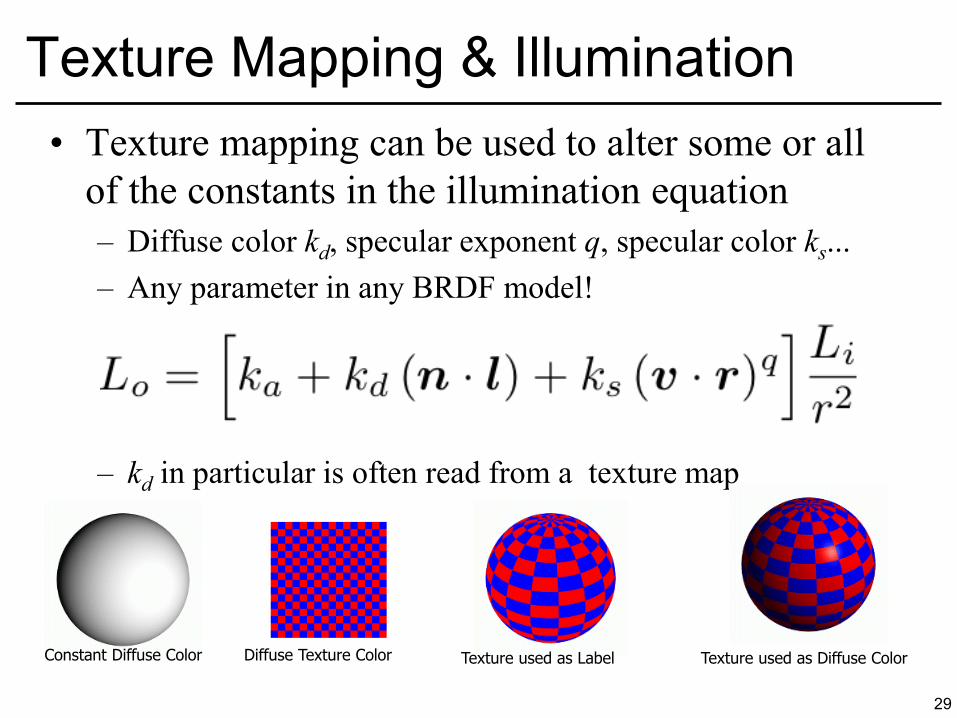
• Texture mapping can be used to alter some or all of the constants in the illumination equation – Diffuse color kd, specular exponent q, specular color ks... – Any parameter in any BRDF model!

– kd in particular is often read from a texture map

29

Texture Mapping & Illumination

Constant Diffuse Color Diffuse Texture Color Texture used as Label Texture used as Diffuse Color

30

Gloss Mapping Example

Spatially varying kd and ks

Ron

Fra

zier

© source unknown. All rights reserved. This content is excluded from our CreativeCommons license. For more information, see http://ocw.mit.edu/help/faq-fair-use/.


31

Questions?

• The normal vector is really important in conveying the small-scale surface detail – Remember cosine dependence – The human eye is really good at

picking up shape cues from lighting!

• We can exploit this and look up also the normal vector from a texture map – This is called “normal mapping” or “bump mapping” – A coarse mesh combined with detailed normal maps can

convey the shape very well! 32

We Can Go Even Further...

• For each shaded point, normal is given by a 2D image normalMap that stores the 3D normal

For a visible point interpolate UV using barycentric

// same as texture mapping Normal = normalMap[U,V] compute shading (BRDF) using this normal

33

Normal Mapping

34

Normal Map Example

Original Mesh 4M triangles

Paolo Cignoni

Image courtesy of Maksim on Wikimedia Commons. License: CC-BY-SA. This content is excluded fromour Creative Commons license. For more information, see http://ocw.mit.edu/help/faq-fair-use/.


http://commons.wikimedia.org/wiki/File:Normal_map_example.png

35

Normal Map Example

Simplified mesh, 500 triangles

Simplified mesh + normal mapping

Paolo Cignoni

Image courtesy of Maksim on Wikimedia Commons. License: CC-BY-SA. This content is excluded fromour Creative Commons license. For more information, see http://ocw.mit.edu/help/faq-fair-use/.


http://commons.wikimedia.org/wiki/File:Normal_map_example.png

36

Normal Map Example

Diffuse texture kd

Normal Map

Final render

Models and images: Trevor Taylor

© source unknown. All rights reserved. This content is excluded from our CreativeCommons license. For more information, see http://ocw.mit.edu/help/faq-fair-use/.

http://www.ttaylormade.com/


37

Generating Normal Maps

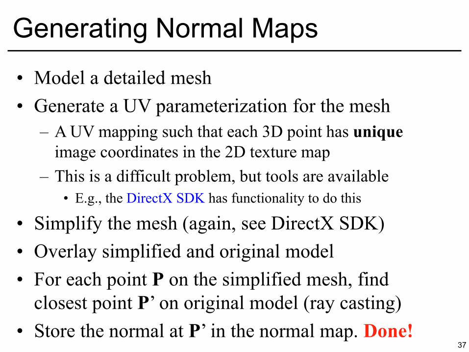
• Model a detailed mesh • Generate a UV parameterization for the mesh

– A UV mapping such that each 3D point has unique image coordinates in the 2D texture map

– This is a difficult problem, but tools are available • E.g., the DirectX SDK has functionality to do this

• Simplify the mesh (again, see DirectX SDK) • Overlay simplified and original model • For each point P on the simplified mesh, find

closest point P’ on original model (ray casting) • Store the normal at P’ in the normal map. Done!

http://msdn.microsoft.com/en-us/directx/default.aspx

• You can store an object-space normal – Convenient if you have a

unique parameterization • ....but if you want to use a tiling normal map, this will not work

– Must account for the curvature of the object!

– Think of mapping this diffuse+normal map combination on a cylindrical tower

• Solution: Tangent space normal map – Encode a “difference” from the

geometric normal in a local coord. system 38

Normal Map Details

39

Questions? Epic Games

Image from Epic Games has been removed due to copyright restrictions.

• Functions executed when light interacts with a surface

• Constructor: – set shader parameters

• Inputs: – Incident radiance – Incident and reflected light directions – Surface tangent basis (anisotropic shaders only)

• Output: – Reflected radiance

40

Shaders (Material class)

• Initially for production (slow) rendering – Renderman in particular

• Now used for real-time (Games) – Evaluated by graphics hardware – More later in the course

• Often makes heavy use of texture mapping

41

Shader

42

Questions?

43

Procedural Textures

Image by Turner Whitted

• Alternative to texture mapping

• Little program that computes color as a function of x,y,z:

f(x,y,z) color

© Turner Whitted, Bell Laboratories. All rights reserved. This content is excluded from ourCreative Commons license. For more information, see http://ocw.mit.edu/help/faq-fair-use/.


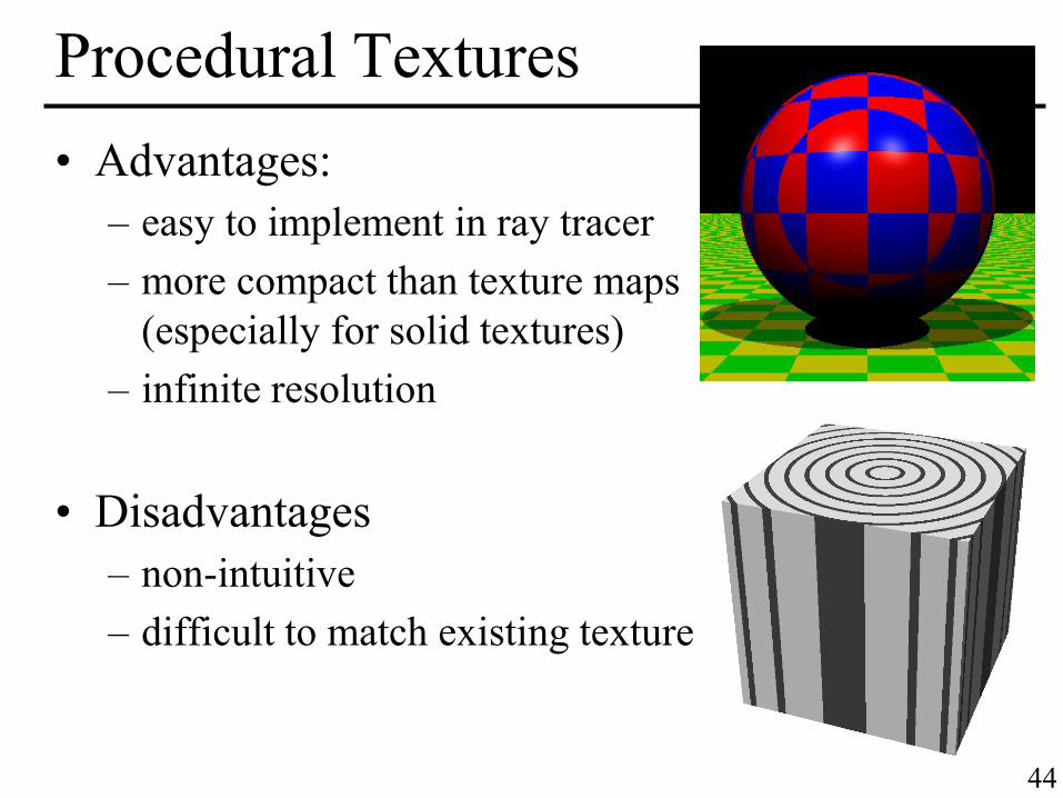
• Advantages: – easy to implement in ray tracer – more compact than texture maps

(especially for solid textures) – infinite resolution

• Disadvantages

– non-intuitive – difficult to match existing texture

44

Procedural Textures

45

Questions?

• Critical component of procedural textures

• Pseudo-random function – But continuous – band pass (single scale)

• Useful to add lots of visual detail http://www.noisemachine.com/talk1/index.html http://mrl.nyu.edu/~perlin/doc/oscar.html http://mrl.nyu.edu/~perlin/noise/ http://en.wikipedia.org/wiki/Perlin_noise http://freespace.virgin.net/hugo.elias/models/m_perlin.htm (not really Perlin noise but very good) http://portal.acm.org/citation.cfm?id=325247

46

Perlin Noise



http://www.noisemachine.com/talk1/index.html

http://mrl.nyu.edu/~perlin/doc/oscar.html

http://mrl.nyu.edu/~perlin/noise/

http://en.wikipedia.org/wiki/Perlin_noise

http://freespace.virgin.net/hugo.elias/models/m_perlin.htm

http://portal.acm.org/citation.cfm?id=325247

• Pseudo random • For arbitrary dimension

– 4D is common for animation • Smooth • Band pass (single scale) • Little memory usage

• How would you do it?

47

Requirements

• Cubic lattice • Zero at vertices

– To avoid low frequencies • Pseudo-random gradient

at vertices – define local linear functions

• Splines to interpolate the values to arbitrary 3D points

48

Perlin Noise

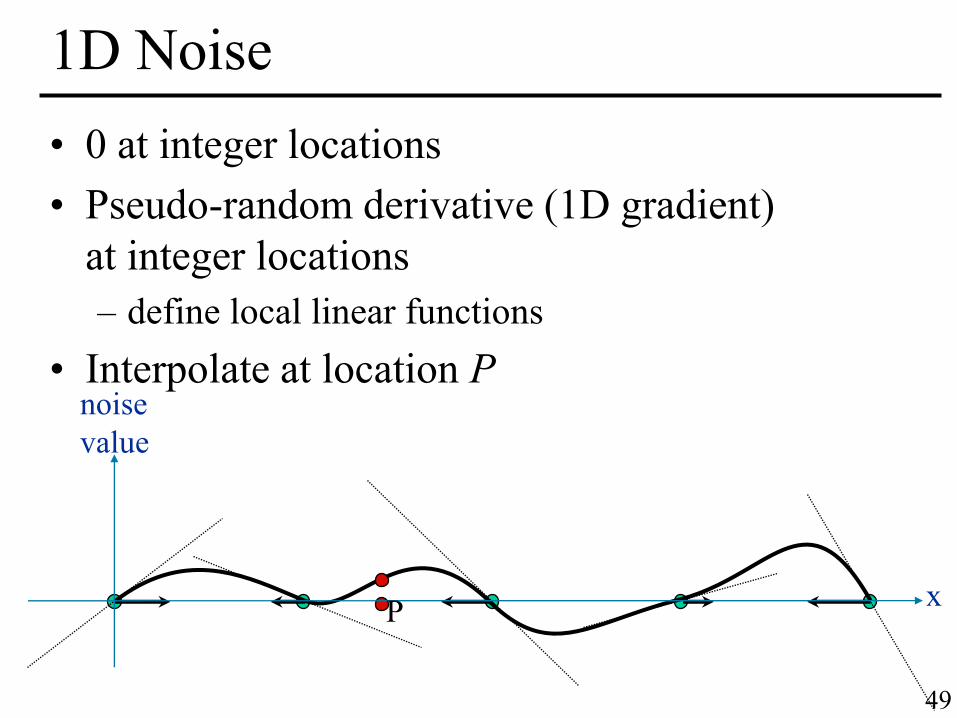
• 0 at integer locations • Pseudo-random derivative (1D gradient)

at integer locations – define local linear functions

• Interpolate at location P

1D Noise

49

noise value

x P

50

1D Noise: Reconstruct at P

noise value

x

dx

G1 G2 P

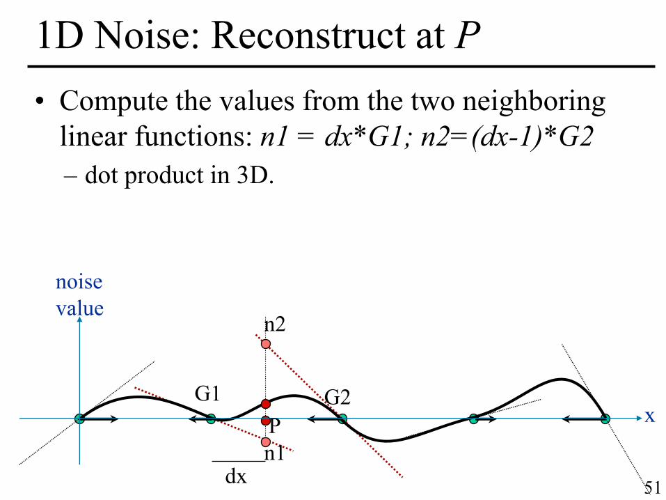
• dx: fractional x coordinate • Gradients G1 and G2 at neighboring vertices

– Scalars in 1D. They are 3D vectors in 3D • We know that noise is zero at vertices

51


noise value

x

dx

G1 G2

n2

n1 P

• Compute the values from the two neighboring linear functions: n1 = dx*G1; n2=(dx-1)*G2 – dot product in 3D.

52


noise value

x

dx

G1 G2

w1 w2 n2

n1 P

• Compute the values from the two neighboring linear functions: n1 = dx*G1; n2=(dx-1)*G2 – dot product in 3D

• Weight w1=3dx2–2dx3 and w2=3(1–dx)2–2(1–dx)3

– ie: noise=w1 G1 dx + w2 G2 (dx-1)

• Given an input point P • For each of its neighboring grid points:

– Get the "pseudo-random" gradient vector G – Compute linear function (dot product G·dP)

• Take weighted sum, using separable cubic weights

– [demo in 2D]

53

Algorithm in 3D

http://www.noisemachine.com/talk1/java/noisegrid.html

• Precompute (1D) table of n gradients G[n] • Precompute (1D) permutation P[n] • For 3D grid point i, j, k :

G(i,j,k) = G[ ( i + P[ (j + P[k]) mod n ] ) mod n ]

• In practice only n gradients are stored! – But optimized so that they are well distributed

54

Computing Pseudo-random Gradients

• A scale is also called an octave in noise parlance

55

Noise At One Scale



• A scale is also called an octave in noise parlance • But multiple octaves

are usually used, where the scale between two octaves is multiplied by 2 – hence the name

octave

56

Noise At Multiple Scales



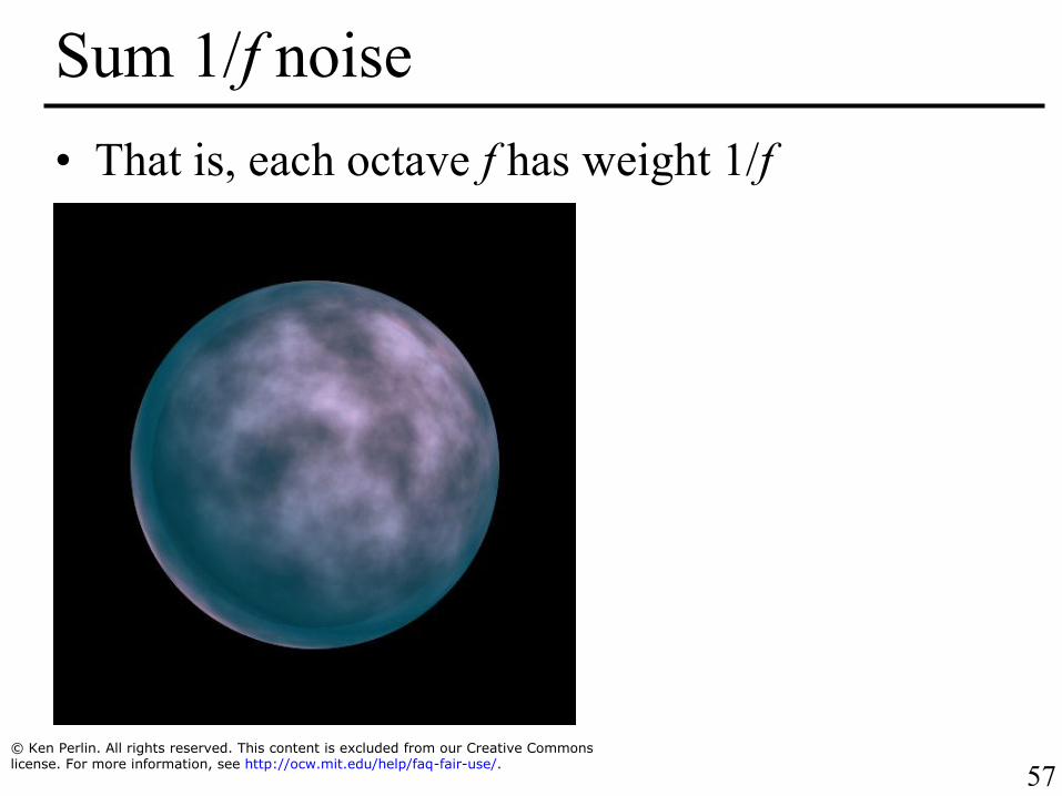
• That is, each octave f has weight 1/f

57

Sum 1/f noise



• Absolute value introduces C1 discontinuities

58

sum 1/f |noise|

• a.k.a. turbulence



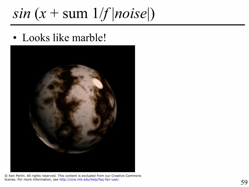
• Looks like marble!

59

sin (x + sum 1/f |noise|)



sum 1/f(noise) sum 1/f( |noise| )

60

Comparison •noise sin(x + sum 1/f( |noise| ))



61

Questions?

• Marble – recall sin (x[0] + sum 1/f |noise|) – BoringMarble = colormap (sin(x[0]) – Marble = colormap (sin(x[0]+turbulence)) – http://legakis.net/justin/MarbleApplet/

• Wood – replace x (or parallel plane)

by radius – Wood = colormap (sin(r+turbulence)) – http://www.connectedpixel.com/blog/texture/wood

62

Noise For Solid Textures

© Ken Perlin. All rights reserved. This content is excludedfrom our Creative Commons license. For more information,see http://ocw.mit.edu/help/faq-fair-use/.


http://legakis.net/justin/MarbleApplet/

http://www.connectedpixel.com/blog/texture/wood

• The corona was made as follows: – Create a smooth gradient function the drops off

radially from bright yellow to dark red. – Phase shift this function by adding a turbulence

texture to its domain. – Place a black cutout disk over the image.

• Animation – Scale up over time – Use higher dim noise (for time) – http://www.noisemachine.com/talk1/imgs/flame500.html

63

Corona

Slides by Ken Perlin

Image of corona removed due to copyright restrictions. Please see the link below for further details.

http://www.noisemachine.com/talk1/imgs/flame500.html

64

Other Cool Usage: Displacement, Fur



65

Questions?

Image removed due to copyright restrictions. Please the image of “blueglass.gif” from http://mrl.nyu.edu/~perlin/imgs/imgs.html.

http://mrl.nyu.edu/~perlin/imgs/imgs.html

• Noise: one ingredient of shaders • Can also use textures • Shaders control diffuse color, but also specular

components, maybe even roughness (exponent), transparency, etc.

• Shaders can be layered (e.g. a layer of dust, peeling paint, mortar between bricks).

• Notion of shade tree – Pretty much algebraic tree

• Assignment 5: checkerboard shader based on two shaders

66

Shaders

• Programmable shader provide great flexibility • Shaders can be extremely complex

– 10,000 lines of code! • Writing shaders is a black art

67

Bottom Line

68

That’s All For Today!

Justin Legakis

Justin Legakis

Courtesy of Justin Legakis.

MIT OpenCourseWarehttp://ocw.mit.edu

6.837 Computer GraphicsFall 2012

For information about citing these materials or our Terms of Use, visit: http://ocw.mit.edu/terms.

http://ocw.mit.edu

http://ocw.mit.edu/terms

Texture Mapping & Shaders - MIT OpenCourseWare · PDF fileTexture Mapping & Shaders ... the...

Documents

Transcript of Texture Mapping & Shaders - MIT OpenCourseWare · PDF fileTexture Mapping & Shaders ... the...