Texas Coastal Wetlands: Status and Trends, mid-1950's to early ...
34
STATUS AND TRENDS, MID-1950s TO EARLY 1990s
Transcript of Texas Coastal Wetlands: Status and Trends, mid-1950's to early ...
STATUS AND TRENDS, MID-1950sTO EARLY 1990s
Shrimp HarvestESTUARINE SYSTEM
STATUS AND TRENDS, MID-1950s TO EARLY 1990s
D. W. MOUlton
March, 1997Texas Parks and Wildlife Department
Austin, Texas
TEXAS PARKS & WILDLIFE DEPARTMENT
T . E . DahlU .S . Fish and Wildlife Service
St . Petersburg, Florida
D . M . Dal]U.S . Fish and Wildlife ServiceAlbuquerque, Ne« , Mexico
TEXASPARKS &
WILDLIFE
United States Department of the InteriorFish and Wildlife ServiceSouthwestern Region
Albuquerque, New Mexico
Cultivated RicePALUSTRINEFARMEDTEXAS PARKS& WILDLIFE DEPARTMENT
Coven'photo:
English/Metric ConversionsRecreational FishingESTUARINE SUBTIDAL
'acre= 0 .4 hectareTEXAS PARKS &WILDLIFEDEPARTMENT
squam me - 2,5),
1 toot = 0.3 meter
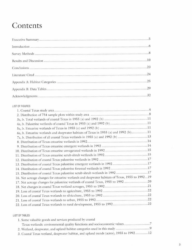
Contents
Executive Summary . . . . . . . . . . . . . . . . . . . . . . . . . . . . . . . . . . . . . . . . . . . . . . . . . . . . . . . . . . . . . . . . . . . . . . . . . . . . . . . . . . . . . . . . . . . . . . . . . . . . . . . . . . . . . . . . . . . . . . . . . .5
Introduction . . . . . . . . . . . . . . . . . . . . . . . . . . . . . . . . . . . . . . . . . . . . . . . . . . . . . . . . . . . . . . . . . . . . . . . . . . . . . . . . . . . . . . . . . . . . . . . . . . . . . . . . . . . . . . . . . . . . . . . . . . . . . . . . . . . .6
Survey Methods . . . . . . . . . . . . . . . . . . . . . . . . . . . . . . . . . . . . . . . . . . . . . . . . . . . . . . . . . . . . . . . . . . . . . . . . . . . . . . . . . . . . . . . . . . . . . . . . . . . . . . . . . . . . . . . . . . . . . . . . . . . . . . .8
Results and Discussion . . . . . . . . . . . . . . . . . . . . . . . . . . . . . . . . . . . . . . . . . . . . . . . . . . . . . . . . . . . . . . . . . . . . . . . . . . . . . . . . . . . . . . . . . . . . . . . . . . . . . . . . . . . . . . . . . . .10
Conclusions . . . . . . . . . . . . . . . . . . . . . . . . . . . . . . . . . . . . . . . . . . . . . . . . . . . . . . . . . . . . . . . . . . . . . . . . . . . . . . . . . . . . . . . . . . . . . . . . . . . . . . . . . . . . . . . . . . . . . . . . . . . . . . . . . . .23
Literature Cited . . . . . . . . . . . . . . . . . . . . . . . . . . . . . . . . . . . . . . . . . . . . . . . . . . . . . . . . . . . . . . . . . . . . . . . . . . . . . . . . . . . . . . . . . . . . . . . . . . . . . . . . . . . . . . . . . . . . . . . . . . . . .24
Appendix A: Habitat Categories . . . . . . . . . . . . . . . . . . . . . . . . . . . . . . . . . . . . . . . . . . . . . . . . . . . . . . . . . . . . . . . . . . . . . . . . . . . . . . . . . . . . . . . . . . . . . . . . . . . . .25
Appendix B : Data Tables . . . . . . . . . . . . . . . . . . . . . . . . . . . . . . . . . . . . . . . . . . . . . . . . . . . . . . . . . . . . . . . . . . . . . . . . . . . . . . . . . . . . . . . . . . . . . . . . . . . . . . . . . . . . . . . .29
Acknowledgments . . . . . . . . . . . . . . . . . . . . . . . . . . . . . . . . . . . . . . . . . . . . . . . . . . . . . . . . . . . . . . . . . . . . . . . . . . . . . . . . . . . . . . . . . . . . . . . . . . . . . . . . . . . . . . . . . . . . . . . . . .32
LIST OF FIGURES
1 . Coastal Texas studv area . . . . . . . . . . . . . . . . . . . . . . . . . . . . . . . . . . . . . . . . . . . . . . . . . . . . . . . . . . . . . . . . . . . . . . . . . . . . . . . . . . . . . . . . . . . . . . . . . . . . . . . . . .42 . Distribution of 754 sample plots within study area . . . . . . . . . . . . . . . . . . . . . . . . . . . . . . . . . . . . . . . . . . . . . . . . . . . . . . . . . . . . . . . . .83a, b. Total wetlands of coastal Texas in 1955 (a) and 1992 (b) . . . . . . . . . . . . . . . . . . . . . . . . . . . . . . . . . . . . . . . . . . . . . . . .114a, b. Palustrine wetlands ofcoastal Texas in 1955 (a) and 1992 (b) . . . . . . . . . . . . . . . . . . . . . . . . . . . . . . . . . . . . . . . . . .115a, b . Estuarine wetlands of Texas in 1955 (a) and 1992 (b) . . . . . . . . . . . . . . . . . . . . . . . . . . . . . . . . . . . . . . . . . . . . . . . . . . . . .116a, b . Estuarine wetlands and deepwater habitats of Texas in 1955 (a) and 1992 (b) . . . . . . . . . . . . . . . . . . I I7a, b . Distribution of all coastal Texas wetlands in 1955 (a) and 1992 (b) . . . . . . . . . . . . . . . . . . . . . . . . . . . . . . . . .138. Distribution of Texas estuarine wetlands in 1992 . . . . . . . . . . . . . . . . . . . . . . . . . . . . . . . . . . . . . . . . . . . . . . . . . . . . . . . . . . . . . . . . . . .149 . Distribution of Texas estuarine emergent wetlands in 1992 . . . . . . . . . . . . . . . . . . . . . . . . . . . . . . . . . . . . . . . . . . . . . . . . . . . 14
10 . Distribution of Texas estuarine unvegetated wetlands in 1992 . . . . . . . . . . . . . . . . . . . . . . . . . . . . . . . . . . . . . . . . . . . . . . . 1511 . Distribution of Texas estuarine scrub-shrub wetlands in 1992 . . . . . . . . . . . . . . . . . . . . . . . . . . . . . . . . . . . . . . . . . . . . . . . . 1512 . Distribution of coastal Texas palustrine wetlands in 1992 . . . . . . . . . . . . . . . . . . . . . . . . . . . . . . . . . . . . . . . . . . . . . . . . . . . . . . 1713 . Distribution of coastal Texas palustrine emergent wetlands in 1992 . . . . . . . . . . . . . . . . . . . . . . . . . . . . . . . . . . . . . . .1714 . Distribution of coastal Texas palustrine forested wetlands in 1992 . . . . . . . . . . . . . . . . . . . . . . . . . . . . . . . . . . . . . . . . .1715 . Distribution of coastal Texas palustrine scrub-shrub wetlands in 1992 . . . . . . . . . . . . . . . . . . . . . . . . . . . . . . . . . . .1716 . Net acreage changes for estuarine wetlands and deepwater habitats ofTexas, 1955 to 1992 . ..1917 . Net acreage changes for palustrine wetlands of coastal Texas, 1955 to 1992 . . . . . . . . . . . . . . . . . . . . . . . . . .2018 . Net changes in coastal Texas wetland acreages, 1955 to 1992 . . . . . . . . . . . . . . . . . . . . . . . . . . . . . . . . . . . . . . . . . . . . . . . . 2119 . Loss of coastal Texas wetlands to agriculture, 1955 to 1992 . . . . . . . . . . . . . . . . . . . . . . . . . . . . . . . . . . . . . . . . . . . . . . . . . .2220 . Loss of coastal Texas wetlands to silviculture, 1955 to 1992 . . . . . . . . . . . . . . . . . . . . . . . . . . . . . . . . . . . . . . . . . . . . . . . . . . 2221 . Loss of coastal Texas wetlands to urban, 1955 to 1992 . . . . . . . . . . . . . . . . . . . . . . . . . . . . . . . . . . . . . . . . . . . . . . . . . . . . . . . . . .2222 . Loss of coastal Texas wetlands to rural development, 1955 to 1992 . . . . . . . . . . . . . . . . . . . . . . . . . . . . . . . . . . . . . . .22
LIST OF TABLES
1 . Some valuable goods and services produced by coastalTexas wetlands : environmental quality functions and socioeconomic values . . . . . . . . . . . . . . . . . . . . . . . . . . . . .7
2 . Wetland, deepwater, and upland habitat categories used in this study . . . . . . . . . . . . . . . . . . . . . . . . . . . . . . . . . . . . . .93 . Coastal Texas wetland, deepwater habitat, and upland trends (acres), 1955 to 1992 . . . . . . . . . . . . . .12

0McAllen
Mid-continent
Plain,nnd
eseamment y
Wharron~
Houston
Beaumont
Upper CoastGaB,Yton . . "8
Texas City
P~ Galveston
Fig . 1Texas Physiographic Regions and Coastal Texas Study Area(comprised of Gulf-Atlantic Coastal Flats and Coastal Zone)

Executive Summary
The U .S . Fish and Wildlife Service prepared thisreport on the status and trends of coastal Texaswetlands in accordance with the CoastalWetlands Planning, Protection, and RestorationAct of 1990 (Title III of Public Law 101-646) .This report is a product of the Coastal TexasProject completed by the Fish and WildlifeService in cooperation with the Texas Parks andWildlife Department and the Texas GeneralLand Office .
This report analyzes data collected for the 12 .8million-acre coastal Texas study area (Fig . 1) .The design of the study consisted of a stratifiedrandom sample of 754 four-square-mile plots .Aerial photographs from the mid-1950s andearly 1990s (mean dates 1955 and 1992) foreach of the plots were analyzed to detect changesin wetlands, decpwater habitats, and uplandsacreage . Changes were determined to be eithernatural or human-induced . The total wetlandsacreage estimate for 1992 was subtracted fromthe 1955 total estimate and divided by the 37-year study period to give an estimate for averageannual net wetlands loss .
An estimated 4.1 million acres of wetlands exist-ed on the Texas coast in the mid-1950s . By theearly 1990s, wetlands had decreased to less than3 .9 million acres including 3 .3 million acres offreshwater wetlands and 567,000 acres of saltwa-ter wetlands . About 1 .7 million acres (52 per-cent) of the 3 .3 million acres of freshwaterwetlands were classified as farmed wetlands . Thetotal net loss of wetlands for the region wasapproximately 210,600 acres, making the aver-age annual net loss of wetlands about 5,700acres . The greatest losses were of freshwateremergent and forested wetlands .
Estuarine (saltwater) wetlands decreased byabout 9.5 percent, with an estimated net loss of59,600 acres, making the average annual net lossapproximately 1,600 acres . Loss of estuarineemergent wetlands occurred primarily betweenFreeport in Brazoria County and Port Arthur inJefferson County . The major cause was faultingand land subsidence, due to withdrawal ofunderground water and oil and gas, which hasresulted in the submergence (drowning) ofmarshes .
Palustrine (freshwater) wetlands showed a netdecline of 151,000 acres (4 .3 percent) .However, this average figure includes a 96,500-acre net increase in palustrine farmed wetlands .
Palustrine emergent wetlands (fresh marsh, wetprairie, etc .) declined by about 29 percent, withan estimated net loss of 235,100 acres, makingthe average annual net loss about 6,400 acres .This was the largest acreage change for any wet-land category studied . Most of the palustrineemergent loss was to upland agriculture andother upland land uses . Also, there was conver-sion of palustrine emergents to the palustrinefarmed and palustrine scrub-shrub wetland types .
Over 96,000 acres (a 10.9 percent decrease) offorested wetlands (swamps, hardwood bottom-lands, etc .) were lost or converted to other wet-land types . Most of the losses were to uplandagriculture and other upland land uses, with con-versions to the palustrine scrub-shrub and palus-trine farmed wetland types and to pcustrinedecpwater (reservoirs) .
Palustrine scrub-shrub wetlands showed a netincrease of over 63,000 acres (a 58 .7 percentincrease) . This increase was primarily at theexpense of palustrine emergent and palustrineforested wetland types . Invasion of fresh marshand cut-over forested wetlands by the introducedChinese Tallow-tree may be responsible formuch of the expansion of scrub-shrub wetlands .
Freshwater ponds showed a net gain of 21,700acres (a 137 percent increase) . About half of theincrease came from conversion of uplands tofarm ponds, stock tanks, and other smallimpoundments . The other half came from con-version of palustrine emergent, palustrinefarmed, and palustrine forested wetlands toponds . The proliferation of man-made pondsobscured the loss ofnatural prairie potholes .
The largest land-use category in the region wasagriculture (4 .7 million acres) . Agriculturalacreage declined by 618,000 acres even though98,000 acres of palustrine wetlands were lost toagriculture . Urban land use increased by529,000 acres, mostly at the expense of agricul-ture and other upland land uses . There was alsoloss of palustrine farmed and other palustrinewetlands to urban and rural development .Approximately 245,000 acres of the upland"other" category, much of it originally nativehardwood and pine-hardwood forest, were con-verted to forested plantation (silviculture) .
Introduction
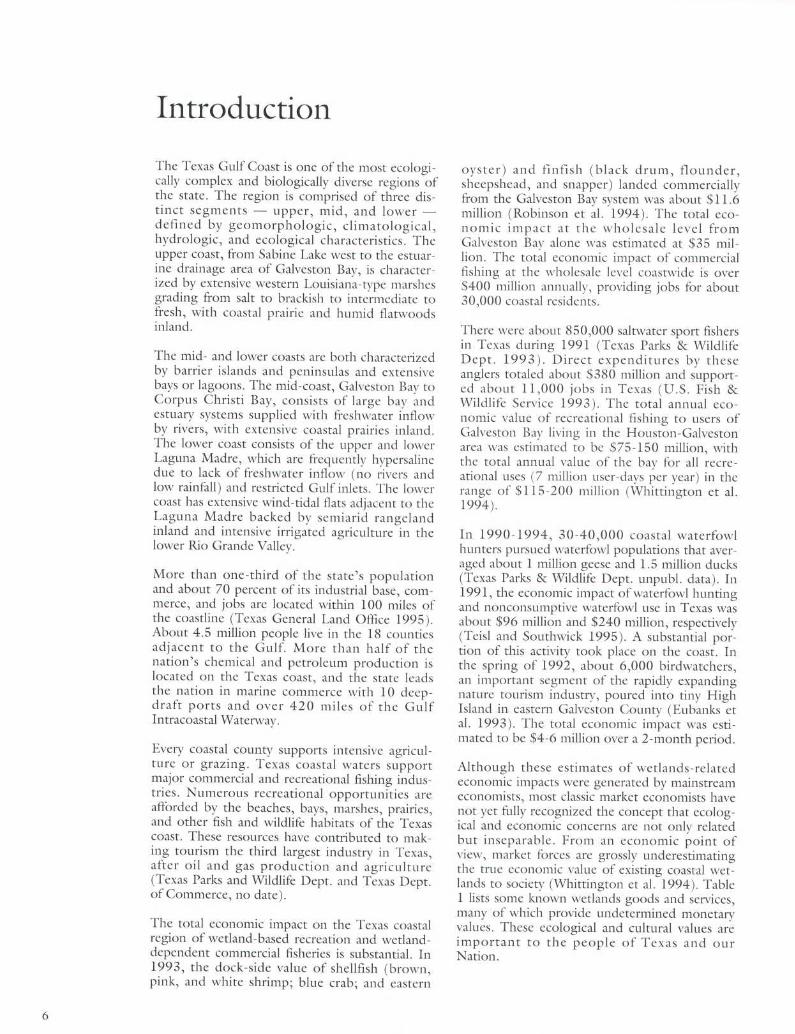
The Texas Gulf Coast is one of the most ecologi-cally complex and biologically diverse regions ofthe state . The region is comprised of three dis-tinct segments - upper, mid, and lower -defined by geomorphologic, climatological,hydrologic, and ecological characteristics . Theupper coast, from Sabine Lake west to the estuar-ine drainage area of Galveston Bay, is character-ized by extensive western Louisiana-type marshesgrading from salt to brackish to intermediate tofresh, with coastal prairie and humid flatwoodsinland .
The mid- and lower coasts are both characterizedby barrier islands and peninsulas and extensivebays or lagoons . The mid-coast, Galveston Bay toCorpus Christi Bay, consists of large bay andestuary systems supplied with freshwater inflowby rivers, with extensive coastal prairies inland .The lower coast consists of the upper and lowerLaguna Madre, which are frequently hypersalincdue to lack of freshwater inflow (no rivers andlow rainfall) and restricted Gulf inlets . The lowercoast has extensive wind-tidal flats adjacent to theLaguna Madre backed by semiarid rangelandinland and intensive irrigated agriculture in thelower Rio Grande Valley .
More than one-third of the state's populationand about 70 percent of its industrial base, com-merce, and jobs are located within 100 miles ofthe coastline (Texas General Land Office 1995) .About 4.5 million people live in the 18 countiesadjacent to the Gulf. More than half of thenation's chemical and petroleum production islocated on the Texas coast, and the state leadsthe nation in marine commerce with 10 deep-draft ports and over 420 miles of the GulfIntracoastal Waterway .
Every coastal county supports intensive agricul-ture or grazing . Texas coastal waters supportmajor commercial and recreational fishing indus-tries . Numerous recreational opportunities areafforded by the beaches, bays, marshes, prairies,and other fish and wildlife habitats of the Texascoast . These resources have contributed to mak-ing tourism the third largest industry in Texas,after oil and gas production and agriculture(Texas Parks and Wildlife Dept . and Texas Dept .of Commerce, no date) .
The total economic impact on the Texas coastalregion of wetland-based recreation and wetland-dependent commercial fisheries is substantial . In1993, the dock-side value of shellfish (brown,pink, and white shrimp ; blue crab ; and eastern
oyster) and finfish (black drum, flounder,sheepshead, and snapper) landed commerciallyfrom the Galveston Bay system was about $11 .6million (Robinson et al . 1994) . The total eco-nomic impact at the wholesale level fromGalveston Bay alone was estimated at $35 mil-lion . The total economic impact of commercialfishing at the wholesale level coastwide is over$400 million annually, providing jobs for about30,000 coastal residents .
There were about 850,000 saltwater sport fishersin Texas during 1991 (Texas Parks & WildlifeDept . 1993) . Direct expenditures by theseanglers totaled about $380 million and support-ed about 11,000 jobs in Texas (U .S . Fish &Wildlife Service 1993) . The total annual eco-nomic value of recreational fishing to users ofGalveston Bay living in the Houston- Galvestonarea was estimated to be $75-150 million, withthe total annual value of the bay for all recre-ational uses (7 million user-days per year) in therange of $115-200 million (Whittington et al .1994) .
In 1990-1994, 30-40,000 coastal waterfowlhunters pursued waterfowl populations that aver-aged about 1 million geese and 1 .5 million ducks(Texas Parks & Wildlife Dept . unpubl . data) . In1991, the economic impact of waterfowl huntingand nonconsumptivc waterfowl use in Texas wasabout $96 million and $240 million, respectively(Teisl and Southwick 1995) . A substantial por-tion of this activity took place on the coast . Inthe spring of 1992, about 6,000 birdwatchers,an important segment of the rapidly expandingnature tourism industry, poured into tiny HighIsland in eastern Galveston County (Eubanks etal . 1993) . The total economic impact was esti-mated to be $4-6 million over a 2-month period .
Although these estimates of wetlands-relatedeconomic impacts were generated by mainstreameconomists, most classic market economists havenot yet fully recognized the concept that ecolog-ical and economic concerns are not only relatedbut inseparable . From an economic point ofview, market forces are grossly underestimatingthe true economic value of existing coastal wet-lands to society (Whittington et al . 1994) . TableI lists some known wetlands goods and services,many of which provide undetermined monetaryvalues . These ecological and cultural values areimportant to the people of Texas and ourNation .
To conserve and manage Texas coastal wetlandsresources, it is necessary to understand thedynamics of the processes, both natural andhuman-induced, that are affecting them . Thisreport presents data that estimate the extent (sta-tus) of Texas coastal wetlands in the early 1990s
and the changes in areal extent (trends) that havetaken place since the mid-1950s . These data mayindicate the impact of existing policies and pro-grams intended to conserve the state's valuablecoastal wetlands resources, and identify whichwetland habitats are experiencing change .
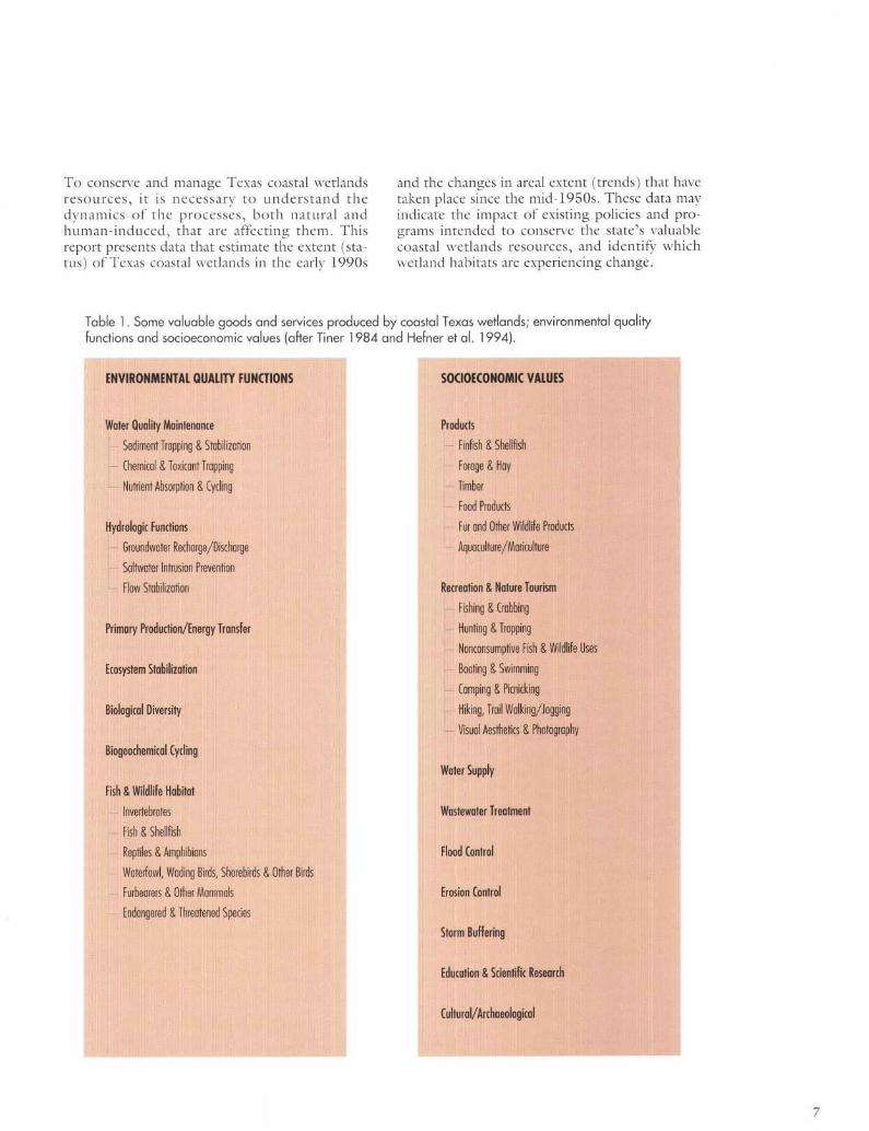
Table 1 . Some valuable goods and services produced by coastal Texas wetlands; environmental qualityfunctions and socioeconomic values (after Tiner 1984 and Hefner et al . 1994).
ENVIRONMENTAL QUALITY FUNCTIONS SOCIOECONOMIC VALUES
Water Quality Maintenance Products
Sediment Trapping & Stabilization Finfish & Shellfish
Chemical & Toxicant Trapping Forage & Hay
Nutrient Absorption & Cycling Timber
Food Products
Hydrologic Functions Fur and Other Wildlife Products
Groundwater Recharge/Discharge Aquaculture/Moriculture
Saltwater Intrusion Prevention
Flow Stabilization Recreation & Nature Tourism
- Fishing & Crabbing
Primary Production/Energy Transfer Hunting & Trapping
Nonconsumptive Fish & Wildlife Uses
Ecosystem Stabilization Boating & Swimming
Camping & Picnicking
Biological Diversity Hiking, Trail Walking/logging
Visual Aesthetics & Photography
Biogeochemical Cycling
Water Supply
Fish & Wildlife Habitat
Invertebrates Wastewater Treatment
Fish & Shellfish
Reptiles & Amphibians Flood Control
Waterfowl, Wading Birds, Shorebirds & Other Birds
Furbearers & Other Mammals Erosion Control
Endangered & Threatened Species
Storm Buffering
Education & Scientific Research
Cultural/Archaeological
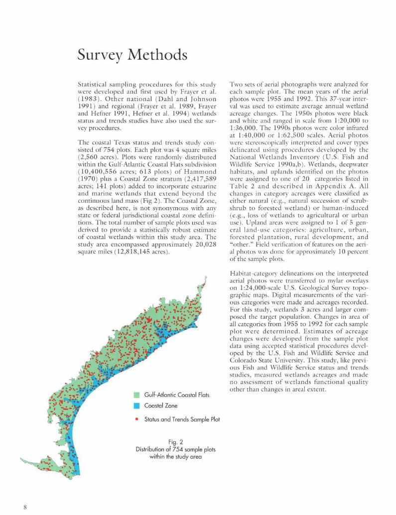
Survey MethodsStatistical sampling procedures for this studywere developed and first used by Frayer et al .(1983) . Other national (Dahl and Johnson1991) and regional (Frayer et al . 1989, Frayerand Hefner 1991, Hefner et al . 1994) wetlandsstatus and trends studies have also used the sur-vey procedures .
The coastal Texas status and trends study con-sisted of 754 plots. Each plot was 4 square miles(2,560 acres) . Plots were randomly distributedwithin the Gulf-Atlantic Coastal Flats subdivision(10,400,556 acres ; 613 plots) of Hammond(1970) plus a Coastal Zone stratum (2,417,589acres; 141 plots) added to incorporate estuarineand marine wetlands that extend beyond thecontinuous land mass (Fig 2) . The Coastal Zone,as described here, is not synonymous with anystate or federal jurisdictional coastal zone defini-tions. The total number of sample plots used wasderived to provide a statistically robust estimateof coastal wetlands within this study area . Thestudy area encompassed approximately 20,028square miles (12,818,145 acres) .
Gulf-Atlantic Coastal Flats
Coastal Zone
"
Status and Trends Sample Plot
Fig. 2Distribution of 754 sample plots
within the study area
Two sets of aerial photographs were analyzed foreach sample plot . The mean years of the aerialphotos were 1955 and 1992 . This 37-year inter-val was used to estimate average annual wetlandacreage changes . The 1950s photos were blackand white and ranged in scale from 1:20,000 to1 :36,000. The 1990s photos were color infraredat 1 :40,000 or 1 :62,500 scales . Aerial photoswere stereoscopically interpreted and cover typesdelineated using procedures developed by theNational Wetlands Inventory (U .S . Fish andWildlife Service 1990a,b) . Wetlands, deepwaterhabitats, and uplands identified on the photoswere assigned to one of 20 categories listed inTable 2 and described in Appendix A. Allchanges in category acreages were classified aseither natural (e.g ., natural succession of scrub-shrub to forested wetland) or human-induced(e .g ., loss of wetlands to agricultural or urbanuse) . Upland areas were assigned to 1 of 5 gen-eral land-use categories : agriculture, urban,forested plantation, rural development, and"other ." Field verification of features on the aeri-al photos was done for approximately 10 percentof the sample plots.
Habitat-category delineations on the interpretedaerial photos were transferred to mylar overlayson 1 :24,000-scale U.S . Geological Survey topo-graphic maps . Digital measurements of the vari-ous categories were made and acreages recorded .For this study, wetlands 3 acres and larger com-posed the target population . Changes in area ofall categories from 1955 to 1992 for each sampleplot were determined . Estimates of acreagechanges were developed from the sample plotdata using accepted statistical procedures devel-oped by the U.S . Fish and Wildlife Service andColorado State University . This study, like previ-ous Fish and Wildlife Service status and trendsstudies, measured wetlands acreages and madeno assessment of wetlands functional qualityother than changes in areal extent .

Table 2 . Wetland, deepwater, and upland habitat categories used in this study . (Detailed descriptions in Appendix A)
Adopted from Cowordin et ol. (1979)
** Deepwater Habitats
***Adopted from Anderson et oL (1976)
Saltwater Habitats* Common Description
Marine Subtidal** Permanent open water of Gulf
Marine Intertidal Shore Gulf beaches, bars, and flats
Estuarine Subtidal** ' Permanent open water of bays
Estuarine Intertidal Emergent Salt, brackish, intermediate marsh
Estuarine Intertidal Scrub-Shrub Baccharis, Black Mangrove, other shrubs
Estuarine Intertidal Unvegetated bay beaches, bars, and flatsUnconsolidated Shore
Freshwater Habitats* Common Description
Palustrine Forested Swamps, hardwood bottomlands, etc .
Palustrine Scrub-Shrub Shrub-sapling wetlands
Palustrine Emergent Fresh marshes, wet prairie, etc .
Palustrine Farmed Cultivated rice fields, some natural wetlands
Palustrine Unconsolidated Shore Unvegetated pond beaches, bars, and flats
Palustrine Unconsolidated Bottom Permanent open water of ponds
Palustrine Aquatic Beds Floating or submerged vegetation
Riverine"` Open water of rivers, streams, canals
Lacustrine** Lakes and reservoirs
Upland Land Use Common Description
Agriculture""" Cropland, pasture, managed rangeland
Urban*** Cities, towns, other densely built-up areas
Forested Plantation Planted or intensively managed forests
Rural Development Nonurban built-up areas and infrastructure
Other Uplands" Nonpatterned native forest, brush, and grassland, barren land
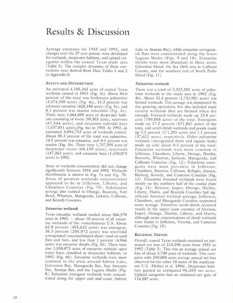
Results & Discussion
Acreage estimates for 1955 and 1992, andchanges over the 37-year period, were developedfor wetlands, deepwater habitats, and upland cat-egories within the coastal Texas study area(Table 3) . The complex dynamics of these con-versions were derived from Data Tables I and 2in Appendix B.
STATUS AND DISTRIBUTION
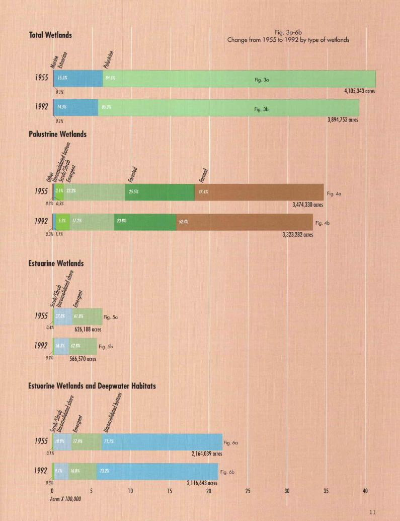
An estimated 4,105,343 acres of coastal Texaswetlands existed in 1955 (Fig . 3a) . About 84.6percent of the total was freshwater palustrine(3,474,330 acres) (Fig . 4a), 15 .3 percent wassaltwater estuarine (626,188 acres) (Fig . 5a), and0 .1 percent was marine intertidal (Fig . 3a) .There were 1,664,698 acres of deepwater habi-tats consisting of rivers (59,303 acres), reservoirs(67,544 acres), and estuarine subtidal bays(1,537,851 acres) ;(Fig. 6a) in 1955 . In 1992, anestimated 3,894,753 acres of wetlands existed .About 85 .3 percent of the total was palustrine,14 .5 percent was estuarine, and 0.1 percent wasmarine (Fig . 36). There were 1,757,595 acres ofdeepwater rivers (60,159 acres), reservoirs(147,363 acres), and estuarine bays (1,550,073acres) in 1992 .
Areas of wetlands concentration did not changesignificantly between 1955 and 1992 . Wetlandsdistribution is shown in Fig. 7a and Fig . 7b .Areas of greatest wetlands concentrationappeared to be in Jefferson, Liberty, andChambers Counties (Fig . 7b) . Substantialacreage also existed in Orange, Brazoria, FortBend, Wharton, Matagorda, Jackson, Calhoun,and Kenedy Counties .
Estuarine wetlands
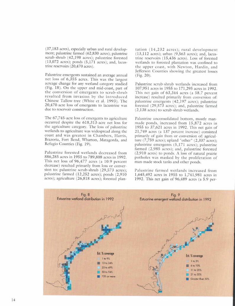
Texas estuarine wetlands totaled about 566,570acres in 1992 - about 10 percent of all estuar-ine wetlands of the conterminous U.S . About62.8 percent (355,632 acres) was emergent,36 .3 percent (205,972 acres) was intertidalunvegetated (unconsolidated shore) mud or sandflats and bars, and less than 1 percent (4,966acres) was estuarine shrubs (Fig . 5b) . There werealso 1,550,073 acres of estuarine subtidal openwater bays, classified as deepwater habitats, in1992 (Fig . 6b) . Estuarine wetlands were mostcommon in the areas around Sabine Lake,Galveston Bay, Matagorda Bay, San AntonioBay, Aransas Bay, and the Laguna Madre (Fig .8) . Estuarine emergent wetlands were concen-trated along the upper and mid-coast (Sabine
Lake to Aransas Bay), while estuarine unvegetat-ed flats were concentrated along the lowerLaguna Madre (Figs . 9 and 10) . Estuarineshrubs were most abundant in three areas :Galveston Island, the Sea Drift area in CalhounCounty, and the southern end of South PadreIsland (Fig . 11).
Palustrine wetlands
There was a total of 3,323,282 acres of palus-trine wetlands in the study area in 1992 (Fig .4b) . About 52 .4 percent (1,741,981 acres) wasfarmed wetlands . This acreage was dominated byrice growing operations, but also included somenatural wetlands that are farmed when dryenough . Forested wetlands made up 23 .8 per-cent (789,808 acres) of the total . Emergentsmade up 17.2 percent (571,867 acres) of thetotal, and scrub-shrub wetlands and ponds madeup 5.2 percent (171,295 acres) and 1 .1 percent(37,621 acres), respectively . Other palustrinewetlands (unvegetated shore and aquatic beds)made up only about 0 .3 percent of the total.Palustrine wetlands were most common inJefferson, Chambers, Liberty, Orange, Hardin,Brazoria, Wharton, Jackson, Matagorda, andCalhoun Counties (Fig . 12). Palustrine emer-gents were most prevalent in Jefferson,Chambers, Brazoria, Calhoun, Refugio, Aransas,Kleberg, Kenedy, and Cameron Counties (Fig .13) . Palustrine forested wetlands were foundmostly on the northern half of the coastal plain(Fig . 14) . Newton, Jasper, Orange, Hardin,Liberty, Harris, and Brazoria Counties had sig-nificant forested wetland acreage; Jefferson,Chambers, and Matagorda Counties supportedsome acreage . Palustrine scrub-shrub occurredmostly in the upper coast counties of Newton,Jasper, Orange, Hardin, Liberty, and Harris,although some concentrations of shrub wetlandswere found in Jefferson, Victoria, and CameronCounties (Fig . 15) .
REGIONAL TRENDS
Overall, coastal Texas wetlands sustained an esti-mated net loss of 210,590 acres from 1955 to1992 (Table 3) . This was an average annual netloss of about 5,700 acres of wetlands . This com-pares with 259,000 acres average annual net lossobserved for the other 10 states of the southeast-ern U.S . (Hefner et al . 1994) . Deepwater habi-tats gained an estimated 96,203 net acres .Upland categories had an estimated net gain of114,387 acres.
Total Wetlands
1955
1992
Palustrine Wetlands
1955
1992
1955
1992
1955
1992
0.1%
0.3 0.5%
0.3% 1.1%
Estuarine Wetlands
0.4%
0.9%
0.1%
Fig . 5a
626,188 acres
Fig . 5b
566,570 acres
Estuarine Wetlands and Deepwater Habitats0 0
haQ ~
00O ~ O
Fig . 6a
2,164,039 acres
Fig . 6b
Fig . 3a-6bChange from 1955 to 1992 by type of wetlands
Fig . 3a
Fig . 3b
Fig. 4a
3,414,330 acres
3,323,282 acres
Fig . 4b
3,894,753 acres
4,105,343 acres
0.3%
2,116,643 acres0
5
10
15
20
25
30
35
40Acres X 100, 000
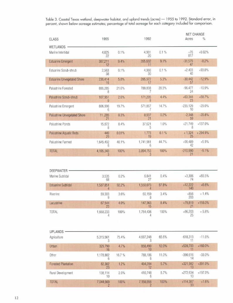
Table 3 . Coastal Texas wetland, deepwater habitat, and upland trends (acres) - 1955 to 1992 . Standard error, in
percent, shown below acreage estimates; percentage of total acreage for each category included for comparison .
NET CHANGE
CLASS 1955 1992 Acres
WETLANDS
Marine Intertidal 4,825 0.1% 4,901 0.1 % +76 +0.02%22 20 817
Estuarine Emergent 387,211 9 4% 355,632 9.1% -31,579 -8 .21%12 11 47
EstLarlre Scrub-shrub 2,563 0.1% 4,966 0.1 % +2,403 +93.8%38 30 40
Estuarine Unvegetated Shore 236,414 5.8% 205,972 5.3% -30,442- -12.9%15 17 57
Palustrlre Forested 886,285 21 .6% 789,808 20.3% -96,477 -10.9%8 7 24
Pal,jstrlne Scrub-shrub 107,951 2.6% 171,295 4.4% +63,344 +58.7%9 9 23
Palustrlne Emergent 806,9966
19.7% 571,8677
14.7% -235,12910
-29.0%
Palustrine Unvegetated Shore 11 ,285 0.3% 8,937 0.2% -2,348 -20.8%21 21 59
Palustrine Pords 15,872 0 .4% 37,621 1 .0% +21,749 +1370%8 5 8
palustrineAquatic Beds 449 0.01% 1,773 0.1 % +1,324 +294.9%29 19 25
PalustrineFarmed 1,645,492 40.1% 1,741,981 44 .7% +96,489 +5.9%6 6 42
TOTAL 4,105,343 100% 3,894,753 100% -210,590 -5 .13 3 21
DEEPWATER
Marine Subtidal 3,535 0.2% 6,841 04% +3,306 +93 .5%68 27 74
Estuarine Subtidal 1,537,851 92.2% 1,550,073 87.8% +12,222 +0.8%4 4 140
Riverine 59,303 3.6% 60,159 3.4% +856 +1 .4%9 8 203
Lacustrine 67,544 4.0% 147,363 8.4% +79,819 +118.0%23 15 21
TOTAL 1,668,233 100% 1,764,436 100% +96,203 +5.8%4 4 25
UPLANDS
Agriculture 5,315,561 75.4% 4,697,248 65.6% -618,313 -11 .6%3 3 11
Urban 329,790 4.7% 858,490 12.0% +528,700 +160.0%16 10 11
Other 1,178,802 16 .7 % 788,186 11 .0% -390,616 -33.0%6 6 14
Forested Plantation 82,302 12 "/, 404,284 5.7% +321,982 +391 .0%23 12 13
Rural Development 138,114 2.0% 410,748 5.7% +272,634 +197.0%10 6 10
TOTAL 7,044,569 100% 7,158,956 100% +114,387 +1 .6%2 2 33
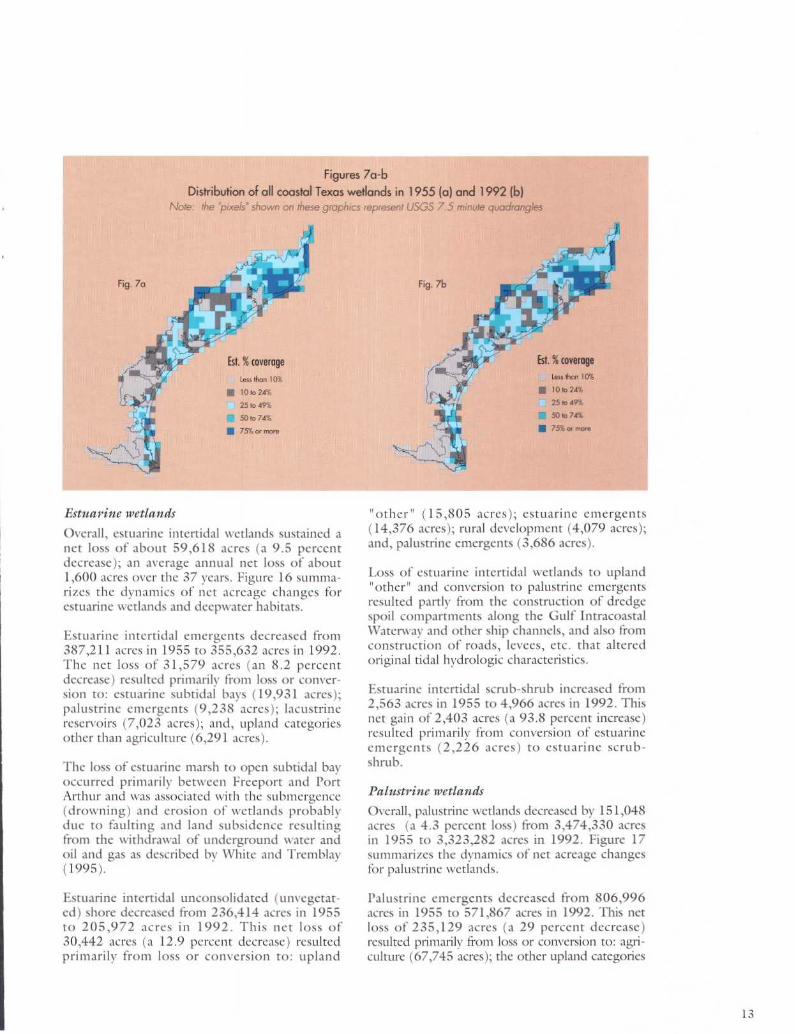
Figures 7a-bDistribution of all coastal Texas wetlands in 1955 (a) and 1992 (b)
Note: the 'pixels" shown on these graphics represent USGS 7.5 minute quadrangles
Fig . 7a
Estuarine wetlands
Est . % coverageLess than 10%
10 to 2490
25 to 49%
50 to 74%
75% or more
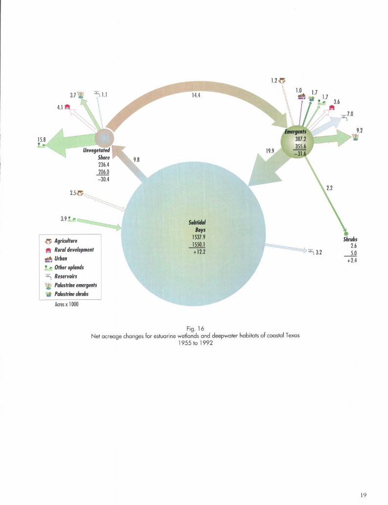
Overall, estuarine intertidal wetlands sustained anet loss of about 59,618 acres (a 9.5 percentdecrease) ; an average annual net loss of about1,600 acres over the 37 years . Figure 16 summa-rizes the dynamics of net acreage changes forestuarine wetlands and dcepNvater habitats .
Estuarine intertidal emergents decreased from387,211 acres in 1955 to 355,632 acres in 1992 .The net loss of 31,579 acres (an 8.2 percentdecrease) resulted primarily from loss or conver-sion to : estuarine subtidal bays (19,931 acres) ;palustrine emergents (9,238 acres) ; lacustrinereservoirs (7,023 acres) ; and, upland categoriesother than agriculture (6,291 acres) .
The loss of estuarine marsh to open subtidal bayoccurred primarily between Freeport and PortArthur and was associates{ with the submergence(drowning) and erosion of Nvetlands probablydue to faulting and land subsidence resultingfrom the withdrawal of underground water andoil and gas as described by White and Tremblay(1995) .
Estuarine intertidal unconsolidated (unvegetat-ed) shore decreased from 236,414 acres in 1955to 205,972 acres in 1992 . This net loss of30,442 acres (a 12 .9 percent decrease) resultedprimarily from loss or conversion to : upland
Fig . 7b
Palustrine wetlands
Est . % coverageLess than 10%
10 to 24%
25 to 49%
.~' 50to74%
75% or more
"other" (15,805 acres) ; estuarine emergents(14,376 acres) ; rural development (4,079 acres) ;and, palustrine emergents (3,686 acres) .
Loss of estuarine intertidal wetlands to upland"other" and conversion to palustrine emergentsresulted partly from the construction of dredgespoil compartments along the Gulf IntracoastalWatenvay and other ship channels, and also fromconstruction of roads, levees, etc . that alteredoriginal tidal hydrologic characteristics .
Estuarine intertidal scrub-shrub increased from2,563 acres in 1955 to 4,966 acres in 1992 . Thisnet gain of 2,403 acres (a 93.8 percent increase)resulted primarily from conversion of estuarineemergents (2,226 acres) to estuarine scrub-shrub .
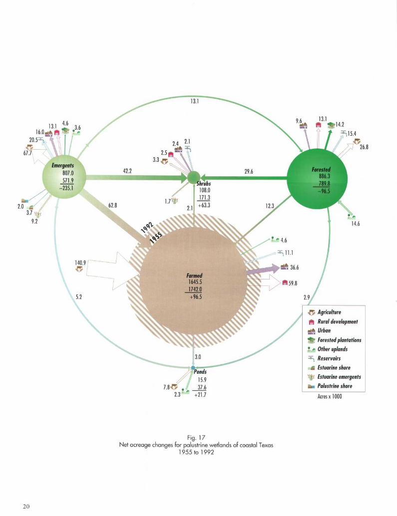
Overall, palustrine wetlands decreased by 151,048acres (a 4 .3 percent loss) from 3,474,330 acresin 1955 to 3,323,282 acres in 1992. Figure 17Summarizes the dynamics of net acreage changesfor palustrine wetlands .
Palustrine emergents decreased from 806,996acres in 1955 to 571,867 acres in 1992 . This netloss of 235,129 acres (a 29 percent decrease)resulted primarily from loss or conversion to : agri-culture (67,745 acres) ; the other upland categories
(37,183 acres), especially urban and rural develop-ment ; palustrine farmed (62,830 acres) ; palustrinescrub-shrub (42,198 acres) ; palustrine forested(13,072 acres) ; ponds (5,171 acres) ; and, lacus-trine reservoirs (20,470 acres) .
Palustrine emergents sustained an average annualnet loss of 6,355 acres . This was the largestacreage change for any wetland category studied(Fig. 18) . On the upper and mid-coast, part ofthe conversion of emergents to scrub-shrubresulted from invasion by the introducedChinese Tallow-tree (White et al . 1993). The20,470-acre loss of emergents to pcustrine wasdue to reservoir construction .
The 67,745-acre loss of emergents to agricultureoccurred despite the 618,313-acre net loss forthe agriculture category . The loss of palustrinewetlands to agriculture was widespread along thecoast and was greatest in Chambers, Harris,Brazoria, Fort Bend, Wharton, Matagorda, andRefugio Counties (Fig . 19) .
Palustrine forested wetlands decreased from886,285 acres in 1955 to 789,808 acres in 1992 .This net loss of 96,477 acres (a 10 .9 percentdecrease) resulted primarily from loss or conver-sion to : palustrine scrub-shrub (29,573 acres) ;palustrine farmed (12,252 acres) ; ponds (2,910acres) ; agriculture (26,818 acres) ; forested plan-
Fig. 8Estuarine wetland distribution in 1992
Est . % coverage1 to 9%
10 to 24%
25 to 49%
50 to 74
75% or more
tation (14,232 acres) ; rural development(13,112 acres) ; urban (9,563 acres) ; and, lacus-trine reservoirs (15,436 acres) . Loss of forestedwetlands to forested plantation was confined tothe upper coast, with Newton, Hardin, andJefferson Counties showing the greatest losses(Fig . 20) .
Palustrine scrub-shrub wetlands increased from107,951 acres in 1955 to 171,295 acres in 1992 .This net gain of 63,344 acres (a 58 .7 percentincrease) resulted primarily from conversion of:palustrine emergents (42,197 acres) ; palustrineforested (29,573 acres) ; and, palustrine farmed(2,138 acres) to scrub-shrub wetlands .
Palustrine unconsolidated bottom, mostly man-made ponds, increased from 15,872 acres in1955 to 37,621 acres in 1992 . This net gain of21,749 acres (a 137 percent increase) consistedprimarily of gain from or conversion of agricul-ture (7,759 acres) ; upland "other" (2,337 acres) ;palustrine emergents (5,171 acres) ; palustrinefarmed (2,985 acres) ; and, palustrine forested(2,910 acres) to ponds. A loss of natural prairiepotholes was masked by the proliferation ofman-made stock tanks and other ponds.
Palustrine farmed wetlands increased from1,645,492 acres in 1955 to 1,741,981 acres in1992 . This net gain of 96,489 acres (a 5.9 per-
Fig . 9Estuarine emergent wetland distribution in 1992
Est . % coverage1 to 51/
6 to 10
11 to 20%
21 to 50%
Greater than 50%

cent increase) consisted primarily of gain from orconversion of: agriculture (140,865 acres) ;palustrine emergents (62,830 acres) ; and, palus-trine forested (12,252 acres) to farmed wetlands .
Most of the palustrine farmed wetlands acreageis in some type of rice production rotation, pri-marily in Wharton, Colorado, Brazoria,Matagorda, Jackson, Jefferson, Chambers,Liberty, and Fort Bend counties . Texas ranksfourth among all states in rice production, withan average annual value in the early 1990s ofabout $150 million (Texas Agricultural StatisticsService 1994) .
There were losses of palustrine wetlands, particu-larly palustrine farmed (96,500 acres) and palus-trine emergents (29,100 acres), to urban andrural development . Loss to urban land use wasgreatest in the Houston and Beaumont-PortArthur areas (Fig . 21) . Loss to rural develop-ment was greatest in Orange, Jefferson,Chambers, Galveston, Harris, Brazoria, andNueces Counties (Fig . 22) .
Deepwater habitatsOverall, deepwater habitats increased by 96,203acres (a 5 .8 percent gain), from 1,668,233 acresin 1955 to 1,764,436 acres in 1992 .
Fig. 10Estuarine unvegetated wetland distribution in 1992
Est . % coverage1 to 5
a 6 to 10%11 to 20%21 to 50
,
Greater than 50%
Estuarine subtidal unconsolidated bottom, i.e .,open water of bays and lagoons, increased from1,537,851 acres in 1955 to 1,550,073 acres in1992 (Fig . 16) . This net gain of 12,222 acres (a0.8 percent increase) resulted primarily fromconversion of: estuarine emergents (19,931acres) ; upland "other" (3,875 acres) ; and, agri-culture (2,461 acres) to subtidal bays . Theseconversions resulted from the submergence anderosion of tidal marshes and bay shorelines most-ly along the upper and mid-coast .
Lacustrine acreage increased from 67,544 acresin 1955 to 147,363 acres in 1992 . This net gainof 79,819 acres (a 118 percent increase) resultedprimarily from conversion of. palustrine emer-gents (20,470 acres) ; palustrine forested (15,436acres) ; palustrine farmed (11,110 acres) ; upland"other" (11,791 acres) ; agriculture (6,409acres) ; and, estuarine intertidal wetlands (8,100acres), mostly emergents, to lacustrine . Theexpansion of the lacustrine category resultedfrom reservoir construction .
Marine subtidal habitats, i.e ., open Gulf water,were included in this study only insofar as theyrelate to losses or gains of the other measuredhabitat categories . For example, the erosion ofGulf beaches would create a loss of marine inter-tidal shore to marine subtidal ; or, the accretion
Fig . 1 1Estuarine scrub-shrub wetland distribution in 1992
Present/sparse
Some estuarine shrubs
Shrubs more common

of sand on a barrier island beach would create aloss of marine subtidal to marine intertidal . Inthat regard, marine subtidal acreage increasedfrom 3,535 in 1955 to 6,841 in 1992 . This netgain of 3,306 acres (a 93 .5 percent increase)resulted primarily from conversion of. marineintertidal beaches (2,044 acres) ; and upland"other" (1,627 acres) to marine subtidal .
Upland categoriesOverall, upland categories increased by 114,387acres (a 1.6 percent gain) from 7,044,569 acresin 1955 to 7,158,956 acres in 1992 .
Upland agriculture decreased from 5,315,561acres in 1955 to 4,697,248 acres in 1992 . Thisnet loss of 618,313 acres (a 11 .6 percentdecrease) resulted primarily from loss or conver-sion to : urban (323,706 acres) ; rural develop-ment (184,633 acres) ; forested plantation(58,891 acres) ; palustrine farmed (140,865acres) ; ponds (7,759 acres) ; and, paustrine reser-voirs (6,409 acres) .
Village Creek, Hardin CountyRIVERINE & PALUSTRINE FORESTEDJIM DICK
Agriculture, the largest land-use category, expe-rienced a 618,313-acre net loss even though98,000 acres of palustrine vegetated wetlands,mostly emergent and forested, were lost to agri-culture, as were 12,000 acres of upland "other."
Upland urban increased from 329,790 acres in1955 to 858,490 acres in 1992 . This gain of528,700 acres (a 160 percent increase) resultedprimarily from conversion of: agriculture(323,706 acres) ; upland "other" (72,271 acres) ;rural development (64,252 acres) ; palustrinefarmed (36,628 acres) ; palustrine emergents(15,966 acres) ; palustrine forested (9,563 acres) ;and, palustrine scrub-shrub (2,425 acres) tourban.
Upland "other," primarily unmanaged or non-patterned forest and rangelands, and barren land,decreased from 1,178,802 acres in 1955 to788,186 acres in 1992 . This net loss of 390,616acres (a 33 percent decrease) resulted primarilyfrom loss or conversion to : forested plantation(244,900 acres) ; urban (72,271 acres) ; ruraldevelopment (53,507 acres) ; agriculture (11,960
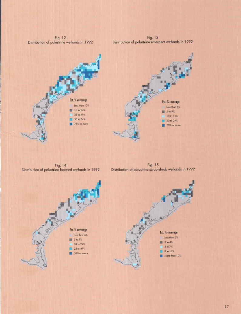
Fig . 12
Fig . 13Distribution of palustrine wetlands in 1992
Distribution of palustrine emergent wetlands in 1992
Est . % coverageLess than 10%
011
10 to 24%
25 to 49%
50 to 74%
75% or more
Est . % coverageLess than 5%
ilpl 5 to 9%
10 to 24%
25 to 49%
50% or more
Est . % coverageLess than 5%
5to9%
10 to 19%
11 .~ 1
20 to 29%
30% or more
Fig . 14
Fig. 15Distribution of palustrine forested wetlands in 1992
Distribution of palustrine scrub-shrub wetlands in 1992
Est . % coverageLess than 3%
3 to 4%
5to7%
8 to 10%
More than 10%
acres) ; palustrine forested (14,570 acres) ; ponds(2,337 acres) ; lacustrine reservoirs (11,791acres) ; and, estuarine subtidal bays (3,875 acres) .Much of the upland "other" acreage that wasconverted to forested plantation was originallynative hardwood and pine-hardwood forest .
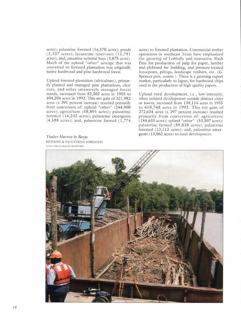
Upland forested plantation (silviculture), primar-ily planted and managed pine plantations, clearcuts, and other intensively managed foreststands, increased from 82,302 acres in 1955 to404,284 acres in 1992 . This net gain of 321,982acres (a 391 percent increase) resulted primarilyfrom conversion of: upland "other" (244,900acres) ; agriculture (58,891 acres) ; palustrineforested (14,232 acres) ; palustrine emergents(4,588 acres) ; and, palustrine farmed (1,774
Timber Harvest by BargeRIVERINE & PALUSTRINE FORESTEDTEXAS PARKS & WILDLIFE DEPARTMENT
acres) to forested plantation . Commercial timberoperations in southeast Texas have emphasizedthe growing of Loblolly and nonnative SlashPine for production of pulp for paper, lumberand plyboard for building, and pressure-treatedfenceposts, pilings, landscape timbers, etc. (G .Spencer pers . comm.) . There is a growing exportmarket, particularly to Japan, for hardwood chipsused in the production of high quality papers .
Upland rural development, i.e ., low-intensity,often isolated development outside distinct citiesor towns, increased from 138,114 acres in 1955to 410,748 acres in 1992 . This net gain of272,634 acres (a 197 percent increase) resultedprimarily from conversion of : agriculture(184,633 acres) ; upland "other" (53,507 acres) ;palustrine farmed (59,838 acres) ; palustrineforested (13,112 acres) ; and, palustrine emer-gents (13,062 acres) to rural development .
3.7
1 .1
4.1 1R~_ 7
3.9 f
2.5 !''
Agriculture
Rural development
Urban
t +^ Other uplands
Reservoirs
Palustrine emergentsPalustrine shrubs
Acres x 1000
14 .4
SubtidalBays
1537 .91550 .1
+12.2
Fig . 16Net acreage changes for estuarine wetlands and deepwater habitats of coastal Texas
1955 to 1992
3.2
2.2
Shrubs2.6
5.0+2 .4
Emergents15 .8 387.2t +° 355.6
Unvegetated 19 .9-31 .6Shore 9.8
236.4
206.0-30.4
16 .020.5
67.7
9 .2
Emergents807 .0571 .9
-235 .1
2 .0
,`
62.8
2.11,
+63 .3
12.33 .7
140 .9
INZ
I
2.4 2.1
13.1
---- _ __ -
Farmed1645 .51742 .0
5 .2
+96.5
Forested886 .3
Shrubs
789.8108 .0
-96.51713.1 .751`
`Ponds15.9
7 .8 ` �
37.62.3 "
+21 .7
Fig . 17Net acreage changes for palustrine wetlands of coastal Texas
1955 to 1992
2 .9
Agriculture
Rural development
Urban
Forested plantations
Other uplands
Reservoirs
Estuarine shoreEstuarine emergentsPalustrine shore
Acres x 1000

0
Palustrine Palustrine Palustrine Palustrine Ponds Other Estuarine Estuarine EstuarineForested Scrub-Shrub Emergent Farmed
Palustrine Emergent Scrub-Shrub Shore
d~0~# +oo,ouu -235,100 =96,500 ~z1,700 -1,000 -31,600 +2,400 -30,400
~;4'IGE ';r, riresl
Bird Watching, Mid-coastESTUARINE SCRUB/SHRUBTI.
PARKS&WILDLIFE DEPARTMENT
Figure 18Changes in coastal Texas wetland acreages, 1955 - 1992

Fig . 19
Fig. 20Loss of coastal Texas wetlands to agriculture
Loss of coastal Texas wetlands to silviculture1955 to 1992
1955 to 1992
Low to none
Moderate
High
0
Insufficient data
Low to none
Moderate
High
Insufficient data
Coastal study boundary
Coastal study boundary
_ _
Coastal study boundary
Fig . 21
Fig. 22Loss of coastal Texas wetlands to urban
Loss of coastal Texas wetlands to rural development1955 to 1992
1955 to 1992
Low to none
Moderate
High
Insufficient data
Low to none
Moderate
High
[]
Insufficient data
Coastal study boundary
ConclusionsWe examined the status of coastal Texas wet-lands at two points in time - the mid-1950sand the early 1990s. The average annual net lossof all vegetated wetlands for that period was5,400 acres. However, federal and state legisla-tion such as the 1948 "Clean Water Act" asamended, the 1969 National EnvironmentalPolicy Act, the 1985 and 1990 "Farm Bills," the1986 Emergency Wetlands Resources Act, the1989 North American Wetlands ConservationAct, the 1981 Texas Waterfowl Stamp Act, the1991 Texas Coastal Coordination Act, and oth-ers, have had a positive influence on wetlandsconservation and management in Texas . Forexample, in the Galveston Bay area, the averagerate of loss of vegetated wetlands decreased fromabout 1,000 acres per year from 1953-1979 toabout 500 acres per year from 1979-1989(White et al. 1993) .
Nevertheless, our results indicate that vegetatedwetlands, particularly freshwater emergent andforested wetlands, are resources that need addi-tional conservation efforts . The acreage losseswithin the upland agriculture and upland"other" categories also give cause for concern.The upland "other" category consists mostly of
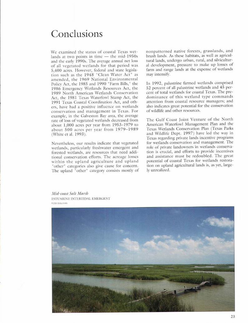
Mid-coast Salt MarshESTUARINE INTERTIDAL EMERGENTROSE SULLIVAN
nonpatterned native forests, grasslands, andbrush lands. As these habitats, as well as agricul-tural lands, undergo urban, rural, and silvicultur-al development, pressure to make up losses offarm and range lands at the expense of wetlandsmay intensify.
In 1992, palustrine farmed wetlands comprised52 percent of all palustrine wetlands and 45 per-cent of total wetlands for coastal Texas. The pre-dominance of this wetland type commandsattention from coastal resource managers ; andalso indicates great potential for the conservationof wildlife and other resources .
The Gulf Coast Joint Venture of the NorthAmerican Waterfowl Management Plan and theTexas Wetlands Conservation Plan (Texas Parksand Wildlife Dept . 1997) have led the way inTexas regarding private lands incentive programsfor wetlands conservation and management . Therole of private landowners in wetlands conserva-tion is crucial, and efforts to provide incentivesand assistance must be redoubled . The greatpotential of coastal Texas for wetlands restora-tion on upland agricultural lands is, as yet, large-ly unrealized .
2 3
Literature Cited
Anderson, J.R, E.E . Hardy, J.T . Roach, and R.E .Witner . 1976 . A land use and land cover classifica-tion system for use with remote sensor data. U.S .Geological Survey Professional Paper 964, U.S .Geological Survey, Washington, D.C .
Cowardin, L.M., V . Carter, F .C . Golet, and E.T .LaRoe . 1979 . Classificatio n of wetlands and deep-water habitats of the United States . U.S . Fish andWildlife Service, FWS/OBS - 79/31, Washington,D.C .
Dahl, T .E . and C.E . Johnson . 1991 . Status andtrends of wetlands in the conterminous UnitedStates, mid-1970's to mid-1980's . U.S . Dept. ofInterior, Fish and Wildlife Service, Washington, D.C .
Eubanks, T.L ., P . Kerfinger, and R.H . Payne . 1993 .High Island : a case study in avitourism . Birding25 :415-420 .
Fraycr, W.E . and J.M . Hefrier . 1991 . Florida Nvet-lands : status and trends, 1970's to 1980's . U.S .Dept . of Interior, Fish and Wildlife Service, Atlanta,GA .
Frayer, W.E ., T.J . Monahan, D.C . Bowden, andF.A . Graybill . 1983 . Status mid trends of wetlandsand deepwater habitats in the conterminous UnitedStates, 1950's to 1970's . Colorado State Univ., FortCollins, CO.
Fraycr, W.E., D.E . Peters, and H .R . Pywell . 1989 .Wetlands of the California Central Valley : status andtrends, 1939 to mid-1980's . U.S . Dept . of Interior,Fish and Wildlife Service, Portland, OR
Hammond, E.H . 1970 . Physical subdivisions of theUnited States ofAmerica. In : National Atlas of theUnited States of America . U.S . Geological Survey,Washington, D .C .
Hefner, J.M., B.O . Wilen, T.E . Dahl, and W.E .Fraycr . 1994 . Southeast wetlands ; status and trends,mid-1970's to mid-1980's . U.S . Dept. of Interior,Fish and Wildlife Service, Atlanta, GA.
Robinson, L., P . Campbell, and L . Butler . 1994 .Trends in Texas commercial fishery landings, 1972-1993 . Management Data Series No . 111, TexasParks and Wildlife Dept., Coastal Fisheries Branch,Austin, TX .
Teisl, M.F . and R . Southwick . 1995 . The economiccontributions of bird and waterfowl recreation inthe United States during 1991 . Southwick Assocs .,Arlington, VA.
Texas Agricultural Statistics Service . 1994 . 1993Texas Crop Statistics . Bull . 252(2), Austin, TX .
Texas General Land Office . 1995 . Texas coastalmanagement program . Austin, TX.
Texas Parks and Wildlife Department . 1993 .Saltwater finfish research and management in Texas :a report to the Governor and the 73rd Legislature .Coastal Fisheries Branch, Austin, TX .
Texas Parks and Wildlife Department. 1997 . Texaswetlands conservation plan . Austin, TX.
Texas Parks and Wildlife Dept. and Texas Dept. ofCommerce . No date . Nature tourism in the LoneStar State ; economic opportunities in nature : areport from the state task force on Texas naturetourism . Austin, TX.
Tiner, R.W., Jr . 1984 . Wetlands of the UnitedStates : current status and recent trends . U.S . Dept .of Interior, Fish and Wildlife Service, Washington,D.C .
U.S . Fish and Wildlife Service . 1990a . Cartographicconventions for the National Wetlands Inventory .St. Petersburg, FL.
U.S . Fish and Wildlife Service . 1990b . Photo inter-pretation conventions for the National WetlandsInventory . St. Petersburg, FL.
U.S . Fish and Wildlife Service . 1993 . 1991 nationalsurvey of fishing, hunting, and wildlife-associatedrecreation : Texas . U.S . Dept. of Interior and U.S .Dept. ofCommerce, U.S . Government PrintingOffice, Washington, D.C .
White, W.A . and T.A . Tremblay . 1995 .Submergence of wetlands as a result of human-induced subsidence and faulting along the upperTexas GulfCoast . J . Coastal Res . 11 :788-807 .
White, W.A., T.A. Tremblay, E .G . Wermund, Jr .,and L.R Handley . 1993 . Trends and status ofwet-land and aquatic habitats in the Galveston Bay sys-tem, Texas . Galveston Bay National Estuary Prog .Pub] . GBNEP-31, Webster, TX.
Whittington, D ., G . Cassidy, D . Amaral, E .McClelland, H . Wang, and C . Poulos . 1994 . Theeconomic value of improving the environmentalquality of Galveston Bay . Galveston Bay NationalEstuary Prog . Publ . GBNEP-38, Webster, TX.
Habitat CategoriesWetland and decpwater habitat categories usedin this report \vere adapted from Cowardin et al .(1979) . In general terms, wetlands arc landswhere saturation with water is the dominant fac-tor determining the nature of soil developmentand the types of plant and animal assemblagesliving in the soil and on its surface . Wetlands arelands transitional between terrestrial and aquaticecosystems where the water table usually is at ornear the surface or the land is covered by shallowwater . The classification system requires thatwetlands have one or more of the followingattributes : 1) at least periodically, the land sup-ports predominantly hydrophytes (water-lovingplants) ; 2) the substrate is predominantlyundrained hydric (water-logged) soil ; and, 3) thesubstrate is nonsoil and is saturated with water orcovered by shallow water at some time duringthe growing season of each year .
Deepwater habitats consist of certain permanent-ly flooded lands . The separation between \vet-land and deepwater habitat in tidal areas coin-cides with the elevation of the extreme low waterof spring tide . In other areas, the separation is ata depth of 2 meters (6.6 feet) below low water .
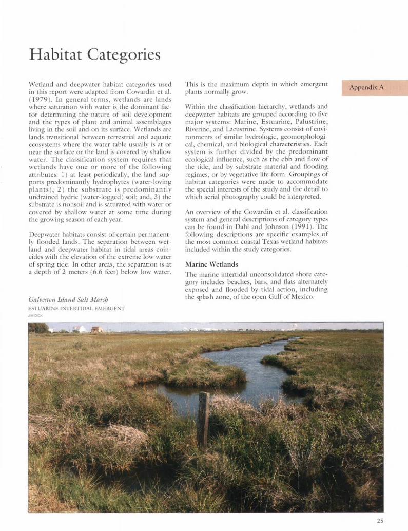
Galveston Island Salt MarshESTUARINE INTERXIDAL EMERGENT
This is the maximum depth in which emergentplants normally grow.
Within the classification hierarchy, wetlands anddeeper,, atcr habitats arc grouped according to livemajor systems : Marine, Estuarine, Palustrine,Riverine, and Lacustrine . Systems consist of envi-ronments of similar hydrologic, geomorphologi-cal, chemical, and biological characteristics . Eachsystem is further divided by the predominantecological influence, such as the ebb and flow ofthe tide, and by substrate material and floodingregimes, or by vegetative life form . Groupings ofhabitat categories were made to accommodatethe special interests of the study and the detail towhich aerial photography could be interpreted .
An overview of the Cowardin et al . classificationsystem and general descriptions of category typescan be found in Dahl and Johnson (1991) . Thefollowing descriptions are specific examples ofthe most common coastal Texas wetland habitatsincluded within the study categories .
Marine WetlandsThe marine intertidal unconsolidated shore cate-gory includes beaches, bars, and flats alternatelyexposed and flooded by tidal action, includingthe splash zone, of the open Gulf ofMexico .
Appendix A
2 5

Estuarine WetlandsThe estuarine intertidal emergent categoryincludes coastal marshes which arc flooded peri-odically by tidal waters with salinity of at ]cast0.5 parts per thousand . The three types of estu-arinc marshes that occur along the Gulf ofMexico are commonly called salt marsh, brackishmarsh, and intermediate marsh . These types canbe separated based on salinity, as reflected by thedominant plant assemblages . Some commonplants of the estuarine marshes include SmoothCordgrass (Spartina alternifora), Saltwort(Batis maritima), Seashore Saltgrass (Distichlisspicata), and Seashore Dropseed (Sporobolus vir-ginicus) in salt marshes ; Black Needlerush(Juneus roemerianus), Marshhay Cordgrass(Spartina patens), and Olney's Bulrush (Scirpusamericanus) in brackish marshes ; and CaliforniaBulrush (Scirpus californicus), Southern Cattail(Typha dowingensis), and Seashore Paspalum(Paspalum vaginatum) in intermediate marshes .
26
The estuarine intertidal scrub-shrub categorydescribes wetlands dominated by woody vegeta-tion and periodically flooded by tidal waters withsalinity of at least 0 .5 parts per thousand . On theTexas coast, this category includes wetlandsdominated by the evergreen shrubs EasternBaccharis (Baccharis halimifolia), Marshelder(Iva frutescens), and on the raid- and lowercoast, Black Mangrove (Avicennia germinans) .Sea Oxeye (Borrichia frutescens), although ashrub, does not appear as such on aerial photosprobably because it often occurs in low, densestands of unbranched plants .
The estuarine intertidal unconsolidated shorecategory includes wetlands with less than 30 per-cent areal coverage by vegetation and periodical-ly flooded by tidal waters with salinity of at least0 .5 parts per thousand . This category includessandbars, mudflats, and other nonvegetated orsparsely vegetated habitats called saltflats .Saltflats are hypersaline environments that gener-ally occur near the interface of salt marsh andupland habitats . Sparse vegetation of saltflatsmay include glassworts (Salicornia spp .),Saltwort, and Shoregrass (Monanthochloe lit-toralis) . Wetlands consisting mostly of sand flatsdominated by algal beds or blue-green algal matsand periodically flooded by astronomic or windtides were also included in this category . Thesehabitats occur extensively on the lower Texascoast along the Laguna Madre .
This study did not include estuarine subtidalaquatic beds (seagrasses) or oyster reefs becausethese habitats cannot always be accurately delin-eated on color infrared aerial photos .
Palustrine WetlandsThe palustrine forested category includes allfreshwater (less than 0 .5 parts per thousandocean-derived salinity) wetlands dominated bywoody vegetation greater than 6 meters (20 feet)in height . Floodplain wetlands called hardwoodbottomlands are the predominant habitat of thiscategory. Water regimes range from brief period-ic flooding to near permanent inundation . Forexample, assemblages dominated by oaks such asOvcrcup Oak (Quercus lyrata), Water Oak(Q nigra), and Willow Oak (Q phellos) alongwith Green Ash (Fraxinus pennsylvanica),Swcetgum (Liquidambar styracifua), and BlackWillow (Salix nigra) are subject to seasonalflooding . Old river channels and oxbows maysupport swamps vegetated predominantly byBald Cypress (Taxodium distichum) and Water-Tupelo (Nyssa aquatica) and may be floodedalmost continuously . Forested wetlands withintermediate degrees of flooding arc an extensivecomponent of the hardwood bottomland spec-trum . Some common trees of the intermediatezones include elms ( Ulmus spp .), Red Maple(Acer rubrum), Water Hickory (Carya aquatica),and Hackberry/Sugar-Berry (Celtis spp .) . Inaddition to hardwood bottomlands, intcrfluvialforested wetlands such as wet pine flatwoods
Cypress Swamp, Orange CountyPALUSTRINE FORESTEDTEXAS PARKS & WILDLIFE DEPT .
dominated by Loblolly Pine (Pinus taeda) coverlarge acreages on the upper Texas coast .
The palustrine scrub-shrub category includes allfreshwater wetlands dominated by woody vege-tation less than 20 feet in height . These habitatsinclude formerly forested wetlands experiencingregrowth or invasion by species such as GreenAsh or the introduced Chinese Tallow-tree(Sapium sebiferum) . This category includesshrub-dominated floodplain depressions, beaverponds, gravel pits, river point-bars, and backwa-ters of ponds and reservoirs vegetated by speciessuch as Swamp Privet (Forestiera acuminata),Brook-side Alder (Alnus serrulata), BlackWillow, ash (Fraxinus caroliniana, F. pennsyl-) ,anica), Buttonbush (Cephalanthus spp .), andPlaner-tree (Planes aquatica) . Chinese Tallow-trce is rapidly invading palustrine emergent wet-lands, including rice fields, on the upper andrnid-coast . Rattlebush (Sesbania spp .) andSaltcedar (Tamarix ramosissinut) arc common indepressions and along drainages throughout thecoastal plain .
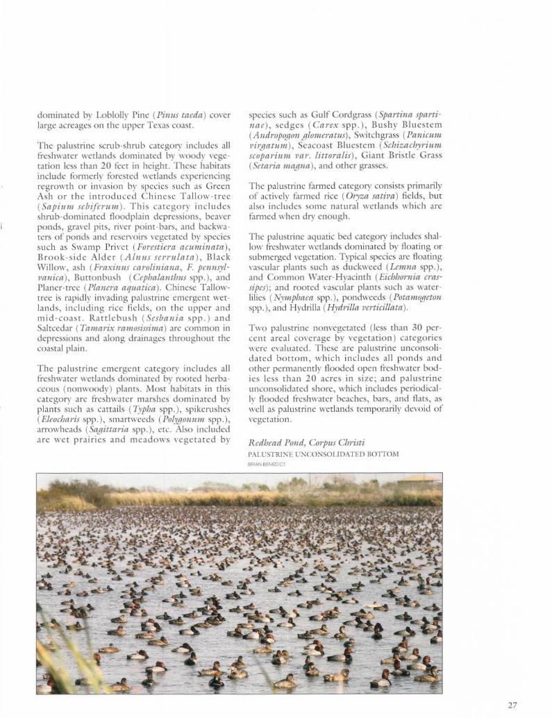
The palustrine emergent category includes allfreshwater wetlands dominated by rooted hcrba-ccous (nonwoody) plants . Most habitats in thiscategory are freshwater marshes dominated byplants such as cattails (Typha spp .), spikerushes(Eleocharis spp .), smartweeds (Po~,Lvjonum spp.),arro,,vheads (Sggittaria spp.), etc . Also includedare wet prairies and meadows vegetated by
species such as Gulf Cordgrass (Spartina sparti-nae), sedges (Carex spp .), Bushy Blucstem(Andropogon glomeratus), Switchgrass (Panicumvirgatum), Seacoast Bluestem (Schizachyriumscoparium var . littoralis), Giant Bristle Grass(Setaria magna), and other grasses .
The palustrine fanned category consists primarilyof actively farmed rice (Oryza sativa) fields, butalso includes some natural -,vetlands which arefarmed when dry enough .
The palustrine aquatic bed category includes shal-low freshwater wetlands dominated by floating orsubmerged vegetation . Typical species are floatingvascular plants such as duckweed (Lemna spp .),and Common Water-Hyacinth (Eichhornia cras-sipes) ; and rooted vascular plants such as water-lilies (Nymphaea spp.), pondweeds (Potamogetonspp .), and Hydrilla (Hydrilla verticillata) .
Two palustrine nonvegetated (less than 30 per-cent areal coverage by vegetation) categoriesNverc evaluated . These are palustrine unconsoli-dated bottom, which includes all ponds andother permanent]\, flooded open freshwater bod-ies less than 20 acres in size ; and palustrineunconsolidated shore, which includes periodical-ly flooded freshwater beaches, bars, and flats, aswell as palustrine wetlands temporarily devoid ofvegetation .
Redhead Pond, Corpus ChristiPAI.I'STRINE UNCONSOUDATED BOTTOMBRIAN BENEDICT

28
Deepwater HabitatsSeveral deepwater habitat categories were includ-ed as they arc the aquatic end of the continuumfor which wetlands function as transitionalzones . These categories are : marine subtidal,where the substrate is permanently submergedby the open Gulf of Mexico ; estuarine subtidal,which includes the permanently submerged areasof bays, lagoons, and lakes where ocean-derivedsalinity exceeds 0.5 parts per thousand, wherethere is at least partial obstruction (barrier islandsor peninsulas) from the open Gulf of Mexico,and there is occasional dilution by freshwaterrunoff from the land ; riverine, which includes allflooded unvegetated freshwater habitats foundwithin a channel ; and lacustrine, which includesall flooded unvegetated freshwater areas of lakesand reservoirs larger than 20 acres .
Houston Ship Channel, Scan Jacinto RiverRIVNRINETEXAS PARKS & WILDLIFE DEPARTMENT
Upland CategoriesAll areas not identified as wetlands or deepwaterhabitats were placed in five upland categories .The agriculture category consists of cropland,pasture, and managed range . The urban catego-n , consists of cities, towns, and other intensivelybuilt-up areas . The "other" uplands category wasadapted from Anderson et al . (1976) . "Other"includes unmanaged or nonpatterned forest landand rangeland, and barren land, as well as landsthat have been drained and cleared but not putto identifiable use . The forested plantation catc-gorv includes planted and managed pine planta-tions, clear cuts, and other intensively managedforests . The rural development category includeslow-density, often isolated development outsidedistinct cities and towns . Rural infrastructureincluding major roads, other transportation,power, and communications facilities, mines andquarries, and golf courses and other recreationalareas u -crc included .
Data TablesEstimates produced include acreages with associ-ated standard errors . Some estimates are notconsidered reliable enough to recommend theiruse for making decisions . An indication of thestatistical reliability of each acreage estimate isgiven in the summary tables included in thisappendix . The standard error of each entryexpressed as a percentage of the entry (SE %) isbelow each acreage estimate . Reliability can bestated generally as : "we are 68 percent confidentthat the true value is within the interval con-structed by adding to and subtracting from theestimate the SE%/100 times the estimate." Forexample, if an estimate is one million acres andthe SE% is 20, then we are 68 percent confidentthat the true value is between 800,000 and1,200,000 acres . An equivalent statement for 95percent confidence can be made by adding andsubtracting twice the amount to and from theestimate . Therefore, a large SE% indicates thatthe estimate has little, if any, reliability . If theSE% is 100 or greater, we can not state that weare 68 percent confident that the true value isnot zero .
This discussion of reliability is meant to aid ininterpretation of the study results . It was expect-ed that only certain estimates would be preciseenough to be meaningful . However, all estimatesare included in the summary tables for additivityand ease of comparison .
Estimates for 1955, 1992, and change over thatperiod were produced for the categoriesdescribed in Appendix A . These estimates aresummarized in Table 1 of Appendix B . Table 2Summarizes estimates by selected surface areagroups . Totals for columns are estimates of totalacreage by category for 1992 . Row totals (thecolumn on the extreme right) are estimates of
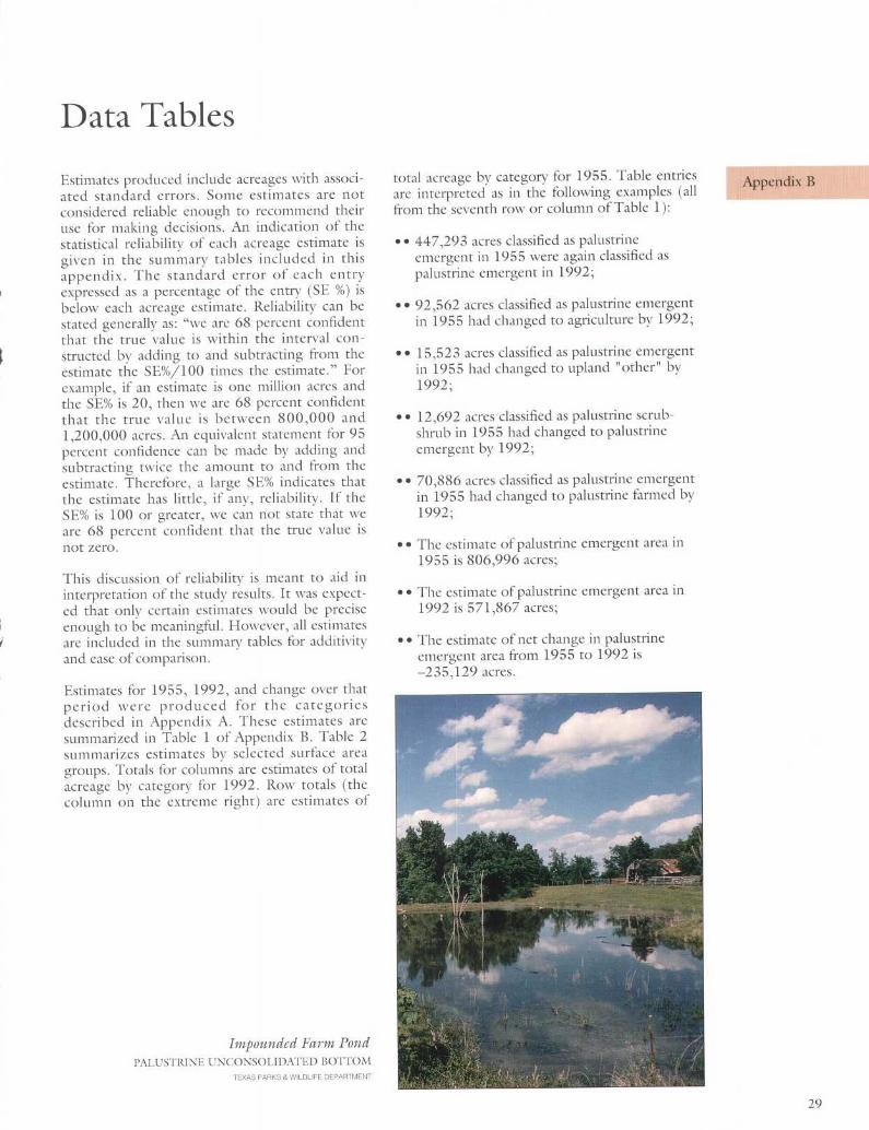
Impounded Farm PondPALUSTRINE UNCONSOLIDATED BOTTOM
TEXAS PARKS & WILDLIFE DEPARTMENT
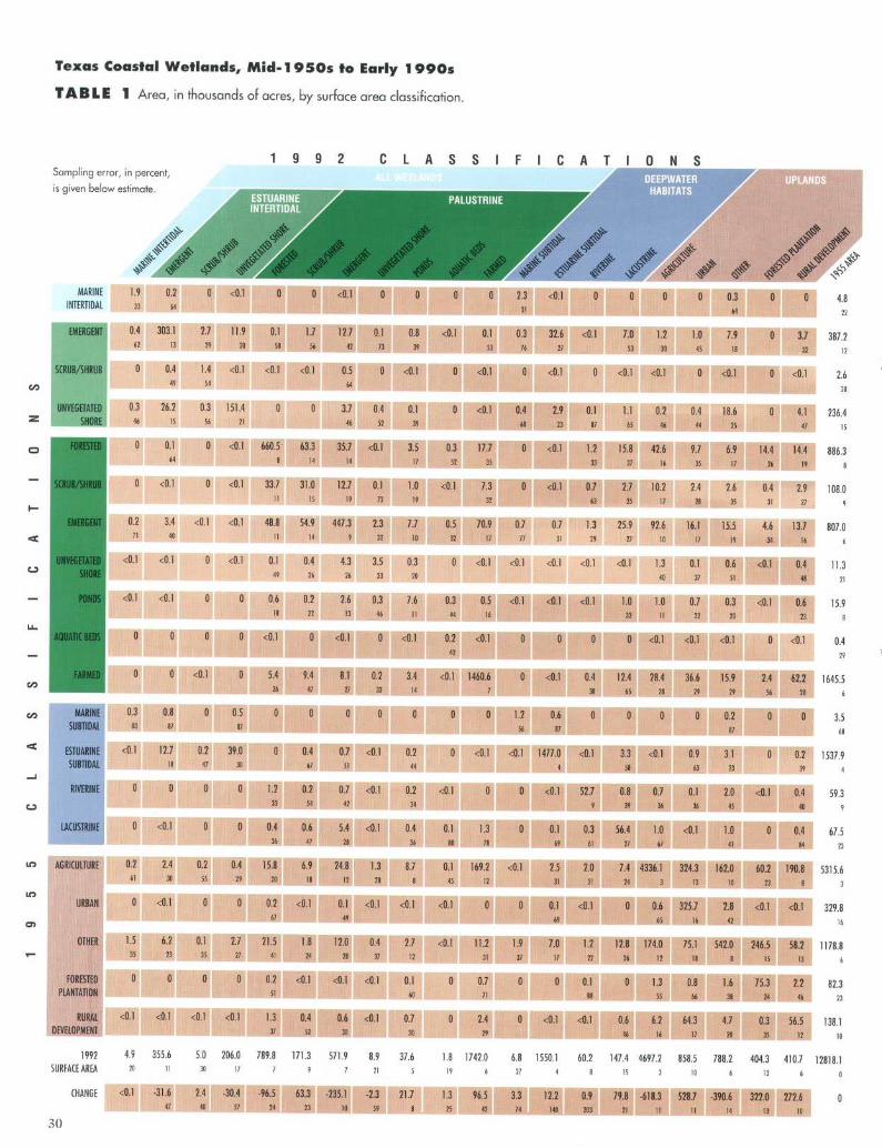
total acreage by category for 1955 . Table entriesare interpreted as in the following examples (allfrom the seventh row or column of Table 1) :
" " 447,293 acres classified as palustrineemergent in 1955 were again classified aspalustrine emergent in 1992;
" " 92,562 acres classified as palustrine emergentin 1955 had changed to agriculture by 1992;
" " 15,523 acres classified as palustrine emergentin 1955 had changed to upland "other" by1992 ;
12,692 acres classified as palustrine scrub-shrub in 1955 had changed to palustrineemergent by 1992;
70,886 acres classified as palustrine emergentin 1955 had changed to palustrine farmed by1992;
" " The estimate ofpalustrine emergent area in1955 is 806,996 acres ;
" " The estimate of palustrine emergent area in1992 is 571,867 acres ;
" " The estimate of net change in palustrineemergent area from 1955 to 1992 is-235,129 acres .
Appendix B
29
CA)
UNVEGETATED 0.3 26 .2 0.3 151 .4 0 0 3.7 0 .4 0.1 0 <0.1 0.4 2.9 0.1 1 .1 0.2 0.4 18 .6 0 4.1 236 .4z
SHORE 46 15 56 21
46 52 39
68 23 87 65 46 44 25
47 15
SCRUB/SHRUB 0 <0.1 0 <0.1 33.7 31 .0 12,7 0 .1 1 .0 <0.1 7 .3 0 <0.1 0 .7 2.7 10 .2 2 .4 2 .6 0 .4 2 .9 108.0.
11
15
19 72
19
32
63
25
17
28
35
31
27
9
Q
SHORE
Q
J
U
Texas Coastal Wetlands, Mid-1950s to Early 1990s
TABLE
1 Area, in thousands of acres, by surface area classification .
Sampling error, in percent,
is given below estimate .
30
EMERGENT
FARMED
MARINE 1 .9 0.2 0 <0.1 0 0 <0 .1 0 0 0 0 2 .3 <0 .1 0 0 0 0 0 .3 0 0 4.8INTERTIDAL 33 64
31
64
22
0.4 303 .1 2 .7 11 .9 0 .1 1 .7 12 .7 0.162 13 29 20 58 56 42 73 39
53 J6 27
53 30 45 18
32
12
SCRUB/SHRUB 0 0 .4 1 .4 <0 .1 <0 .1 <0 .1 0.5 0 <0 .149 54
64
FORESTED 0 0.1 0 <0.1 660 .5 63.3 35.7 <0 .1 3.5 0.3 17.7 0 <0.1 1 .2 15 .8 42 .6 9 .7 6 .9 14 .4 14 .4 886.364
8
14
14 ,.
17
52
35
'' 33 . . .
37
16
35
17
26
19
8
EMERGENT 0 .2 3.4 <0 .1 <0.1 48.8 54 .9 447 .3 2.3 7 .7 0 .5 70.9 0 .7 0 .7 1 .3 25.9 92 .6 16 .1 15.5 4 .6 13.7 807 .071
40
11
14
9 32
10
32
17
77
31
29
27
16
17
19
34
16
6
UNVEGETATED <0 .1 <0.1 0 <0 .1 0 .1 0 .4 4 .3 3.5 0 .3 0 <0 .1 <0 .1 <0 .1 <0 .1 <0 .1 1 .3 0.1 0.6 <0.1 0.4 11 .349 26
26 33 20
40 37 51
48
21
PONDS <0.1 <0 .1
0
0 0 .6 0.2 2:6 0 .3 7.6
0 .3 0.5 <0 .1 41< '<0.1 1 .0 1 .0 0.7 0.3 <0.1 0.6 15 .918
22
13 46
11
44
16
32 11
22
20
23
8
AQUATIC BEDS
0
0
0
0
<0 .1
0
<0.1
0
<0.1
0.2
<0.1
0
0
0
0
<0 .1
<0 .1
<0 .1
0
<0 .1
0.442
29
0 0 0 1 .2 0 .6 0 0 0 0 0 .2 0 0 3 .5SUBTIDAL 83 87
87
56 87
87 68
ESTUARINE <0 .1 12.7 0 .2 39 .0 0 0 .4 0 .7 <0.1 0 .2 0 <0 .1 41 1477 .0 <0 .1 3 .3 <0 .1 0 .9 3.1 0 0.2 1531 .9SUBTIDAL
18 47 30
67 51
44
4
58
63 23
39
4
RIVERINE
LACUSTRINE
URBAN
OTHER
<0 .1
AGRICULTURE
0.2 2 .4 0.2 0 .4 15 .8 6.9 24.8 1 .3 8.7
0.1 169.2 <0.1
2.5 2.0 7 .4 4336 .1 324 .3 162 .0 60 .2 190 .8 5315.661
30
55
29
20
18
12 28
8
45
12
31
21
24
3
13
10
23
8
3
1 .5 6 .235 23
1 9 9 2 C L A S S I F I C A T I 0 N S
0 <0.1 0 5.4 9 .4 8.1 0 .2 3.4 <0.1 1460.6 0 <0.1 0 .4 12 .4 28 .4 36 .6 15 .9 2 .4 62,2 1645.527 33 14
7
38 65 28 29 29
56 20
6
36 47
28
36
88
78
69 61
27 67
41
84
23
Sl0. J0
~~ '`L~O
k~F~G~CC~~ O~~EG~P~OSQ~O`'
POOPS\~Q+`r05PQ~kO
10cQ
O~
~
P -§P
0 .3 32 .6 <0 .1 7 .0 1 .2 1 .0 7.9 0 3.7 387 .2
y3O`y`t4~
~OQ``SStO
00O~
Sg55P~FP
<0.1 2 .6
0 .2 0 .7 <0 .1 0 .2 <0 .1 0 0 <0 .1 52 .7 0 .8 0.7 0.1 2.0 <0.1 0.4 59 .354 47
34
9 39 36 36 45
40
9
0,6 ` 5.4 <0 .1
0.4
0.1
1 .3
0
0.1
0.3
56 .4
1 .0
<0.1
1 .0
0
0 .4
67 .5
1 01 <0.1 <0.1 <0.1 0 0 0 .1 <0 .1 0 0 .6 325 .7 2 .8 <0 .1 <0 .1 329.869
65
16
42
16
12 .0 0.4 2 .7 <0 .1 11 .2 1 .9 7 .0 1 .2 12.8 174 .0 75.1 542.0 2465 58.2 1178 .828 37
12
31
37
17
22
36
12
18
8
15
13
6
FORESTED 0 0 0 0 0 .2 <0 .1 <0 .1 <0 .1 0 .1 0 0 .7 0 0 0 .1 0 1 .3 0.8 1 .6 75.3 2.2 82 .3PLANTATION
51
60
71
88
55 66 38 24 46 23
RURAL <0.1 <0 .1 <0 .1 <0 .1 1 .3 0.4 0.6 <0 .1 0.7 0 2.4 0 <0.1 <0.1 0 .6 6.2 64.3 4.7 0.3 56.5 138 .1DEVELOPMENT
37 52 30
30
29
46 16 17 20 35 12 10
1992
4.9 355 .6 5.0 206 .0 789 .8 171 .3 571 .9 8 .9 37.6
1 .8 1742.0 6 .8 1550 .1 60 .2 147 .4 4697 .2 858 .5 788 .2 404 .3 410 .7 12818 .1SURFACEAREA
20
11
30 17
7
9
7 21
5
19
6 27
4
8
1s
3
10
6
12
6
0
CHANGE <0 .1 -31 .6 2 .4 -30.4 -96.5 63 .3 .235 .1 -2 .3 21 .7 1 .3 96 .5 3 .3 12 .2 0 .9 79.8 -618 .3 528 .7 -390 .6 322 .0 272 .6
047
40
57
24
23
10 59
8
25
42
74
140 203
21
11
11
14
13
10

Texas Coastal Wetlands, Mid-1950s to Early 1990s
TABLE 2
Area, in thousands of acres, by selected surface area groups .
Sampling error, in percent,
is given below estimate .
Duck HuntingPALUSTRINE EMERGENTTEXAS PARKS & WILDLIFE DEPARTMENT
1 9 9 2 C L A S S I I'l CATIONS
MARINE
ESTUARINE
PALUSTRINE
1955 AREA
h
zMARINE 1 .9
0 .2
<0.1
2 .4
0 .3
4 .8
0
33
67
31
64
22
a ESTUARINE 0.7
497.4
20 .3
70.7
37 .1
626 .2
V
43
10
34
17
16
9
PALUSTRINE 0 .2
3 .7
3007 .7
63 .1
399 .7
3474.3N
68
38
4
70
7
3N
a0 .3
53 .1
12 .2
1592 .4
10 .2
1668 .2
81
23
18
4
17
4
`n
1 .8
12 .2
283 .1
35.8
6711 .6
7044 .6
34
1s
8
15
2
2
1992 AREA
4 .9
566 .6
3323 .3
1764 .4
7159 .0
12818 .1
20
9
4
4
2
0
CHANGE <0 .1
59 .6
151.1
96 .2
114.4
37
26
25
33
3 1
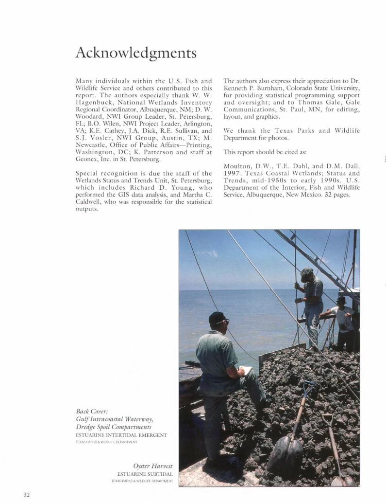
AcknowledgmentsMany individuals within the U.S . Fish andWildlife Service and others contributed to thisreport . The authors especially thank W. W.Hagenbuck, National Wetlands InvcntorvRegional Coordinator, Albuquerque, NM; D . W.Woodard, NWI Group Leader, St . Petersburg,FL; B .O . Wilen, NWI Project Leader, Arlington,VA; K.E . Cathcy, J.A . Dick, R.E . Sullivan, andS .J . Vosler, NWI Group, Austin, TX ; M.Newcastle, Office of Public Affairs-Printing,Washington, DC ; K. Patterson and staff atGconex, Inc. in St . Petersburg .
Special recognition is due the staff of theWetlands Status and Trends Unit, St . Petersburg,which includes Richard D. Young, whoperformed the GIS data analysis, and Martha C.Caldwell, who was responsible for the statisticaloutputs.
GulfIntracoastal Waterivay,Dredge Spoil CompartmentsESTUARINE INTERTIDAI . FAIER
Oyster HarvestESTUARINE SUBTIDAL
TEXAS PARKS& WILDLIFE DEPARTMENT
The authors also express their appreciation to Dr .Kenneth P. Burnham, Colorado State University,for providing statistical programming supportand oversight; and to Thomas Gale, GaleCommunications, St . Paul, MN, for editing,layout, and graphics .
We thank the Texas Parks and WildlifeDepartment for photos .
This report should be cited as :
Moulton, D.W ., T .E . Dahl, and D .M . Dall .1997 . Texas Coastal Wetlands; Status andTrends, mid-1950s to early 1990s . U .S .Department of the Interior, Fish and WildlifeService, Albuquerque, New Mexico . 32 pages.

Al