Tests for m-dependence based on sample splitting methods · PDF fileTests for m-dependence...

Ins t i tu t ional Reposi tory

This document is published in:

Journal of Econometrics, 173, 143-159, 2013

DOI: http://dx.doi.org/10.1016/j.jeconom.2012.11.005

© Elsevier

Tests for m-dependence based on SampleSplitting Methods∗

Seongman Moon † Carlos Velasco ‡

Universidad Carlos III de Madrid Universidad Carlos III de Madrid

November 6, 2012

Abstract

This paper develops new test methods for m-dependent data. Our ap-

proach is based on sample splitting by regular sampling of the original data

at lower frequencies, so that standard techniques for testing independence

can be used for each individual subsample. We then propose several alterna-

tive statistics that aggregate information across subsamples and investigate

their asymptotic and finite sample properties. We apply our methods to test

the predictability of excess returns in foreign exchange markets. We also il-

lustrate how our serial dependence tests can provide useful information for

identifying particular economic alternatives when testing the expectations

hypothesis in foreign exchange markets.

Keywords: m-dependence, sample splitting, pooled method, Wald method,

minimum/maximum/median method, expectations hypothesis.

JEL Classification: C14, F31, F37

∗We are grateful to Associate Editor and two anonymous referees for helpful comments andsuggestions.†Department of Economics, Universidad Carlos III de Madrid, Calle Madrid 126, 28903 Getafe

Madrid, SPAIN. Email: [email protected], Tel.: +34-91-624-8668, Fax: +34-91-624-9329. Re-search support from Spanish Secretary of Education (SEJ2007-63098) is gratefully acknowledged.‡Department of Economics, Universidad Carlos III de Madrid, Calle Madrid 126, 28903 Getafe

Madrid, SPAIN. Email: [email protected], Tel.: +34-91-624-9646, Fax: +34-91-624-9329.Research support from the Spanish Plan Nacional de I+D+I (SEJ2007-62908) is gratefully ac-knowledged

1

1 Introduction

In many contexts it is known or assumed that economic time series are m-

dependent. We say that a stochastic process Xt∞t=−∞ is m-dependent if for some

integer m ≥ 0 and every n, the collections

. . . , Xn−1, Xn and Xn+m+1, Xn+m+2, . . .

are independent. In such cases, usual independence is equivalent to 0-dependence.

m-dependence arises when data are sampled more finely than the forecasting in-

terval (or maturity) for testing the expectations or the efficient market hypotheses,

when differencing methods are applied to remove fixed effects, or when evaluating

the goodness-of-fit of a moving average (MA) model.

Our paper is inspired by testing the predictability of k-month ahead excess

returns, which is a key step when investigating the expectations hypotheses of for-

ward exchange rates or of the term structure of interest rates.1 If data are sampled

more finely, for example monthly, than the forecasting horizon, the forecasting er-

rors then display a MA structure and become m-dependent (or (k−1)-dependent,

in this example) under the expectations hypothesis.2 To take into account this

dependency, Hansen and Hodrick (1980) examined restrictions on a k-step ahead

forecasting regression and proposed corrected standard errors (see also Newey and

West (1987)). Researchers, however, have faced difficulties in applying their meth-

ods to tests that are designed only for independent data. For instance, Campbell

and Dufour (1995) had to assume that forecasting errors are independent to de-

velop tests of orthogonality based on signs and signed ranks. Escanciano and

Velasco (2006) who used nonlinear test methods also had to assume unpredictable

forecasting errors. The conditional test by Jansson and Moreira (2006) and the

Q-test by Campbell and Yogo (2006) are other examples of this issue.

In this paper we develop new testing methods for m-dependent data. Our

approach first splits the original time series into m + 1 subsamples so that the

observations within each subsample are independent under the null hypothesis of

1See Engel (1996) and Lewis (1995) for a survey of tests for the expectations hypothesis inforeign exchange markets; and see Campbell and Shiller (1991) and Cochrane and Piazzesi (2005)for tests of the expectations hypothesis of the term structure of interest rates.

2We use the notation of m-dependence for the general concept and (k − 1)-dependence fora specific example throughout the paper. The notation of m-dependence is from the statisticalliterature and the notation of k is from the expectations hypothesis literature.

2

m-dependence. Then, we apply standard techniques for testing uncorrelation to

the individual subsamples. However, m-dependence induces correlation between

the subsamples that must be accounted for when constructing test statistics to

aggregate information from the subsamples.

To apply our sample splitting methods, we focus on linear methods based on

the autocorrelations most stressed in practice.3 In particular, we apply them to

three common serial dependence tests: the variance ratio, the Box-Pierce portman-

teau, and the Fama-French (1988) tests. Specifically, we first propose Wald type

statistics exploiting joint distributions across subsamples. Second, we use Bonfer-

roni bounds to control the size of the tests based on one-sided maximal deviations.

Third, we design new statistics that pool estimates from individual subsamples.

To improve the finite sample behavior of these test procedures, we design a para-

metric bootstrap method that accounts for the effects of the m-dependence and

show that it provides very good size accuracy even with long return horizons, for

which the asymptotic normal approximation usually performs poorly.

Our sample splitting methods have several advantages for addressingm-dependent

data compared to previous studies. The residual-based methods using parameter

estimates can be subject to estimation errors. For example, for testing a lin-

ear MA(m) model, the asymptotic distribution of goodness-of-fit statistics based

on residuals autocorrelation might depend on the estimation method employed.4

Regression-based methods also need to account for this serial dependence through

different variants of autocorrelation robust standard errors. In contrast, our sam-

ple splitting methods guarantee exact independence of the data under the null

hypothesis of m-dependence because they do not estimate (or even specify) para-

metric models. Dufour and Torres (1998) proposed sample splitting in the context

of regression-based tests, but used bound methods to conduct asymptotic infer-

ence, while we explicitly account for the dependence among subsamples avoiding

possible efficiency losses due to these approximations.

We also distinguish our methods from the typical long-horizon tests based on

variance ratios for the random walk hypothesis of asset prices.5 These tests mainly

3Our approach can also permit different characterizations of the independence hypothesis,including the martingale difference and the white noise hypotheses.

4Those statistics include the Box-Pierce, the LM, and the Tp statistics. See Delgado andVelasco (2011) for a recent discussion.

5See, for example, Lo and MacKinlay (1988) and Poterba and Summers (1988) for stock

3

differ from ours in terms of the assumption of m-dependent data. The random

walk assumption always implies 0-dependence, regardless of how finely the data

are sampled. However, maturities (or forecasting intervals) in the expectations

hypothesis induce m-dependence components in excess returns. In this case, the

expected value of the usual variance ratio statistic is no longer 1, and is left unspec-

ified. Therefore, direct application of this and related predictability tests requires

adjusting the sampling time interval to maturity to guarantee uncorrelated re-

turns under the expectations hypothesis. Consequently, this approach leads to

inefficiencies due to an effectively reduced sample size and poses a new problem of

aggregating information if several subsamples are used instead.

The rest of the paper is organized as follows. Section 2 presents the asymp-

totic theory of our sample splitting methods and Section 3 provides the parametric

bootstrap procedures. We employ the sample splitting methods to tests for the

expectations hypothesis in foreign exchange markets in Section 4 and discuss their

size and power properties in Section 5. An empirical study for testing the ex-

pectations hypothesis in foreign exchange markets is provided in Section 6 and

concluding remarks follow.

2 The Asymptotic Theory of Sample Splitting Methods form-dependent Data

In this section, we present sample splitting methods for m-dependent data in

the context of testing the expectations hypothesis. We first characterize the notion

of the lack of linear predictability beyond a forecasting horizon k and introduce

further assumptions that lead to exact (k − 1)-dependence. We then provide the

asymptotic properties of the serial dependence tests implemented in the presence

of m-dependent data. We begin with the typical variance ratio test. To compare

our methods with previous studies, we briefly state the distributional results of

the variance ratios when k = 1. Here, k = 1 means that the variance test assumes

0-dependent data under the null hypothesis. Then, we analyze the asymptotic

properties of the variance ratio tests when k > 1. Furthermore, we show that the t

statistics of Fama-French (1988) belong to the class of generalized variance ratios,

and we analyze their asymptotic properties in this context. We also apply our

methods to the Box-Pierce (1970) portmanteau Q statistics. Finally, we relate our

prices, Liu and He (1991) for spot exchange rates, and Cochrane (1988) for the U.S. output.

4

results to previous studies and discuss the applications of our methods to other

tests, possibly capturing nonlinear dependence.

Let S = ξ1|k, ξ2|k, . . . , ξT |k be the original sample, where ξt|k denotes the k-

period excess return between period t − k and t. Suppose a researcher wants to

test the predictability of excess returns beyond horizon k. Then, the data become

(k − 1)-dependent under the null hypothesis, and the usual methods for testing

uncorrelation or independence cannot be used directly. For example, if data are

collected at a monthly frequency and the researcher wants to forecast excess returns

for a holding period of three-months, then k = 3. To address this dependence, we

propose sample splitting methods. The main idea of our procedure is to first di-

vide the original sample into k subsamples in the following way. Define each of the

k subsamples by S1 = ξ1|k, ξk+1|k, . . . , ξT−k+1|k, S2 = ξ2|k, ξk+2|k, . . . , ξT−k+2|k,. . ., Sk = ξk|k, ξ2k|k, . . . , ξT |k. Here, a subsample is constructed such that all

ξt|k are uncorrelated or unpredictable within the subsample under the null of no

predictability but a subsample itself is correlated with other subsamples. Then

we use the usual tests for uncorrelation or independence for each subsample. Fi-

nally, we propose several methods that aggregate information across the subsample

statistics.

2.1 An Econometric Framework

Assume that the k-period excess returns ξt|k are covariance stationary and have

autocorrelation sequence γk(i) = Cov(ξt|k, ξt+i|k)/V ar(ξt|k) satisfying γk (i) = 0 for

|i| ≥ k. Then, from the Wold decomposition, it holds that

H(k)0 : ξt+k|k = αk +

k∑i=1

ciet+i,

where et is weak noise, i.e., E [et] = 0, E [e2t ] = σ2 and E [etet−i] = 0 for any

i 6= 0, and σ2k = V ar

(ξt|k)

= σ2∑k

i=1 c2i > 0. Thus ξt|k follows a weak linear

MA (k − 1) model. Here, the hypothesis implies that information in or prior to

ξt|k is not useful to forecast ξt+k|k linearly and that the autocorrelation function is

truncated. However, the hypothesis does not restrict the possibility of nonlinear

relationships in higher order moments at any horizon. So et still can be nonlinearly

predictable at any horizon or can display conditional dynamic heteroscedasticity.

To build asymptotic theory on sample autocorrelations and variance ratios,

5

we need to further restrict the dependence of the innovation process et. For this,

we impose mixing conditions plus one assumption on the higher joint moments

restricting the form of a possible ARCH structure, using Assumption H∗ of Lo and

MacKinlay (1988) provided next.

Assumption 2.1 .

1. For all t, E [et] = 0 and E [etet−τ ] = 0 for any τ 6= 0.

2. et is φ-mixing with coefficients φ(j) of size r/(2r− 1) or is α-mixing with

coefficients α(j) of size r/(r − 1), where r > 1, such that for all t and for

any τ ≥ 0, there exists some δ > 0 for which E|etet−τ |2(r+δ) < ∆ <∞.

3. limT→∞1T

∑Tt=1E [e2t ] = σ2 <∞.

4. For all t, any nonzero j and i where j 6= i

E[e2t et−jet−i

]= 0. (1)

Assumption 2.1 guarantees that the linear projection of ξt+k|k given ξt|k, ξt−1|k, . . .

is constant. The mixing conditions in Assumption 2.1.2 can be replaced by a

martingale difference assumption stating that E [et|et−1, et−2, . . .] = 0 for all t.

This martingale assumption on et would imply that the process ξt|k is not pre-

dictable beyond horizon k under H(k)0 , i.e., the conditional expectation of ξt+k|k

given ξt|k, ξt−1|k, . . . is constant. Note that (1) allows for deterministic changes in

the variance and for ARCH effects. In general, this condition implies that the

sample autocorrelation coefficients of et at different lags are asymptotically uncor-

related, despite the presence of heteroscedasticity. Based on condition (1), Lo and

MacKinlay (1988) propose robust estimates of the asymptotic variance of autocor-

relation coefficients that lead to asymptotic normal feasible inference for variance

ratio tests. If we further impose the homoscedasticity of et, the asymptotic variance

expressions simplify, as is the case when we strengthen the dependence conditions

on et to exact independence as in the next assumption.

Assumption 2.2 et is an iid random variable with mean zero, variance σ2 and

finite fourth moment.

6

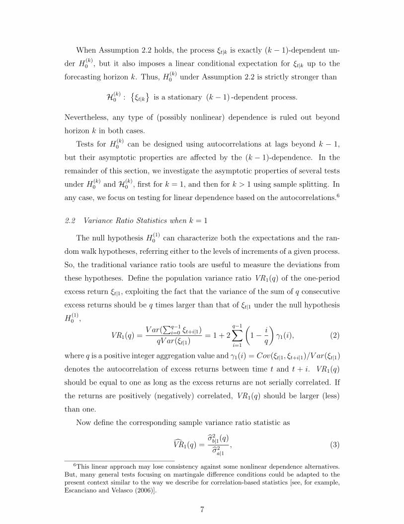
When Assumption 2.2 holds, the process ξt|k is exactly (k − 1)-dependent un-

der H(k)0 , but it also imposes a linear conditional expectation for ξt|k up to the

forecasting horizon k. Thus, H(k)0 under Assumption 2.2 is strictly stronger than

H(k)0 :

ξt|k

is a stationary (k − 1) -dependent process.

Nevertheless, any type of (possibly nonlinear) dependence is ruled out beyond

horizon k in both cases.

Tests for H(k)0 can be designed using autocorrelations at lags beyond k − 1,

but their asymptotic properties are affected by the (k − 1)-dependence. In the

remainder of this section, we investigate the asymptotic properties of several tests

under H(k)0 and H(k)

0 , first for k = 1, and then for k > 1 using sample splitting. In

any case, we focus on testing for linear dependence based on the autocorrelations.6

2.2 Variance Ratio Statistics when k = 1

The null hypothesis H(1)0 can characterize both the expectations and the ran-

dom walk hypotheses, referring either to the levels of increments of a given process.

So, the traditional variance ratio tools are useful to measure the deviations from

these hypotheses. Define the population variance ratio VR1(q) of the one-period

excess return ξt|1, exploiting the fact that the variance of the sum of q consecutive

excess returns should be q times larger than that of ξt|1 under the null hypothesis

H(1)0 ,

VR1(q) =V ar(

∑q−1i=0 ξt+i|1)

qV ar(ξt|1)= 1 + 2

q−1∑i=1

(1− i

q

)γ1(i), (2)

where q is a positive integer aggregation value and γ1(i) = Cov(ξt|1, ξt+i|1)/V ar(ξt|1)

denotes the autocorrelation of excess returns between time t and t + i. VR1(q)

should be equal to one as long as the excess returns are not serially correlated. If

the returns are positively (negatively) correlated, VR1(q) should be larger (less)

than one.

Now define the corresponding sample variance ratio statistic as

VR1(q) =σ2b|1(q)

σ2a|1

, (3)

6This linear approach may lose consistency against some nonlinear dependence alternatives.But, many general tests focusing on martingale difference conditions could be adapted to thepresent context similar to the way we describe for correlation-based statistics [see, for example,Escanciano and Velasco (2006)].

7

where σ2b|1(q) = (qg1(q))

−1∑Tt=q(ξt|1+ξt−1|1+· · ·+ξt−q+1|1−qα1)

2 and σ2a|1 = σ2

b|1(1).

Here, T is sample size, g1(q) = (T−q+1)(1−q/T ) corrects the bias in the variance

estimator σ2b|1(q) under the null, and α1 = T−1

∑Tt=1 ξt|1. Because the mean and

variance of the q consecutive returns are linear in the aggregation interval q under

the null hypothesis H(1)0 , σ2

b|1(q) is an unbiased estimate of the variance of a single

return. In this sense, the variance ratio test on uncorrelated excess returns shares

the essence of the random walk hypothesis test, which exploits that the variance

of random walk increments must be a linear function of the time interval.

Based on Lo and MacKinlay’s (1988) analysis, a variance ratio test for the

expectations hypothesis can be easily developed so that

z1(q) =√T(

VR1(q)− 1)(2(2q − 1)(q − 1)

3q

)− 12

follows the standard normal distribution asymptotically under H(1)0 and Assump-

tion 2.2, and further t statistics can be developed under Assumption 2.1.

Note that economic theories for both hypotheses do not explicitly guide the

choice of q. In the long-horizon predictability tests for the random walk of asset

prices, the choice of large values of q is motivated by the desire to detect the effect

of a highly persistent component in asset prices on the return predictability and

thus to improve the power of these tests. However, in principle, q = 2 can be

enough to test the expectations hypothesis, but examining the serial dependence

pattern across different q can provide useful information for the identification of

an alternative hypothesis as discussed in Section 4. Regardless of the objectives of

the study, the choice of q in both tests involves the use of overlapping observations

as is explicit in the definition of σ2b|1(q). However, as shown in detail below, the

nature of the dependence arising in this context is different from that induced by

subsampling when k > 1. One of our objectives in this paper is to address this

difference.

2.3 Variance Ratio Statistics when k > 1

The above approach can only be used for the case in which the maturity or

the forecasting interval exactly matches the sampling time interval. However, it is

not uncommon for researchers to use data that are sampled more finely than the

forecasting interval or maturity for testing the predictability of excess returns. In

8

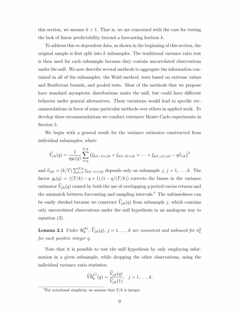
this section, we assume k > 1. That is, we are concerned with the case for testing

the lack of linear predictability beyond a forecasting horizon k.

To address thism-dependent data, as shown in the beginning of this section, the

original sample is first split into k subsamples. The traditional variance ratio test

is then used for each subsample because they contain uncorrelated observations

under the null. We now describe several methods to aggregate the information con-

tained in all of the subsamples: the Wald method, tests based on extreme values

and Bonferroni bounds, and pooled tests. Most of the methods that we propose

have standard asymptotic distributions under the null, but could have different

behavior under general alternatives. These variations would lead to specific rec-

ommendations in favor of some particular methods over others in applied work. To

develop these recommendations we conduct extensive Monte Carlo experiments in

Section 5.

We begin with a general result for the variance estimates constructed from

individual subsamples, where

Vj|k(q) =1

qgk(q)

T/k∑t=q

(ξk(t−1)+j|k + ξk(t−2)+j|k + · · ·+ ξk(t−q)+j|k − qαj|k

)2and αj|k = (k/T )

∑T/kt=1 ξk(t−1)+j|k depends only on subsample j, j = 1, . . . , k. The

factor gk(q) = ((T/k)− q + 1) (1− q/(T/k)) corrects the biases in the variance

estimator Vj|k(q) caused by both the use of overlapping q-period excess returns and

the mismatch between forecasting and sampling intervals.7 The unbiasedness can

be easily checked because we construct Vj|k(q) from subsample j, which contains

only uncorrelated observations under the null hypothesis in an analogous way to

equation (3).

Lemma 2.1 Under H(k)0 , Vj|k(q), j = 1, . . . , k are consistent and unbiased for σ2

k

for each positive integer q.

Note that it is possible to test the null hypothesis by only employing infor-

mation in a given subsample, while dropping the other observations, using the

individual variance ratio statistics:

VR(j)

k (q) =Vj|k(q)

Vj|k(1), j = 1, . . . , k.

7For notational simplicity we assume that T/k is integer.

9

However, a single subsample contains only T/k observations, which is a fraction

of the original sample. Instead, our modified approaches shown below increase

the effective sample size by k times and can yield important efficiency gains. For

example, k is 3 when monthly observations are used for testing the three-month

excess return predictability but k becomes 13 when weekly observations are used.

To exploit simultaneously all VR(j)

k (q) available in a given data set, we consider

the asymptotic joint distribution of

Uk(q) =

√T/k√

2(q − 1)(2q − 1)/3q

(VR

(1)

k (q)− 1, . . . , VR(k)

k (q)− 1)′. (4)

Denote as δ(a,b)k (i, j) the asymptotic covariance of sample autocorrelations at lags

i and j across the different subsamples a and b,

δ(a,b)k (i, j) = ACov

((T/k)1/2γ

(a)k (i), (T/k)1/2γ

(b)k (j)

).

Lemma 2.2 Under H(k)0 ,

Uk(q) ∼a N (0,Σk(q)) ,

where the diagonal elements of Σk(q) > 0 are 1, and in general, 1 ≤ b ≤ a ≤ k,

Σk(q)[a,b] =

1

σ4k

q−1∑i=1

(1− i

q

)2

δ(a,b)k (i, i)

+

q−1∑i=2

(1− i

q

)(1− i− 1

q

)[δ(a,b)k (i, i− 1) + δ

(a,b)k (i− 1, i)

],

with σ2k = V ar(ξt|k) and

δ(a,b)k (i, i) = E

[ξ0ξa−bξikξik+a−b

]+ E

[ξ0ξa−b−kξikξik+a−b−k

], i > 0;

δ(a,b)k (i, i− 1) = E

[ξ0ξa−bξikξik+a−b−k

], i > 1;

δ(a,b)k (i, i+ 1) = E

[ξ0ξa−b−kξikξik+a−b

], i > 0; (5)

for ξt = ξt|k − αk, and δ(a,a)k (i, j) = 0, i 6= j; δ

(a,b)k (i, j) = 0, |i− j| > 1.

The correlation among different subsamples is reflected in the terms depending

on δ(a,b)k (i, j) for a 6= b in Σk(q). However, if a = b, δ

(a,a)k (i, i) = E

[ξ20]E[ξ2ik]

=

E[ξ20]2

= σ4k, but δ

(a,a)k (i, j) = 0 for i 6= j under H(k)

0 so that Σk(q)[a,a] = 1,

recovering the usual result under independence, k = 1.

10

In general, for any a, b, and i > 1, the first element in δ(a,b)k (i, i) factorizes under

H(k)0 , i.e., E

[ξ0ξa−bξikξik+a−b

]= E

[ξ0ξa−b

]E[ξikξik+a−b

]= E

[ξ0ξa−b

]2, but does

not factorize when i = 1 because it is not possible to isolate pairs of independent

random variables in E[ξ0ξa−bξkξk+a−b

]. However, all other expectations in Σk(q)

factorize for all values of i indicated:

E[ξ0ξa−b−kξikξik+a−b−k

]= E

[ξ0ξa−b−k

]E[ξ0ξk−a+b

]= E

[ξ0ξa−b−k

]2, i > 0;

δ(a,b)k (i, i− 1) = E

[ξ0ξa−b

]E[ξ0ξa−b−k

], i > 1;

δ(a,b)k (i, i+ 1) = E

[ξ0ξa−b−k

]E[ξ0ξa−b

], i > 0,

so that the right hand side of the above three terms does not depend on i, and the

estimation of Σk(q) is simplified under H(k)0 .

If we impose linearity, but allow for general dynamic heteroscedasticity, the

basic results on the asymptotic distribution of Uk hold, but Σk(q) is affected. In

particular, under H(k)0 , condition (1) implies that E

[ξ2t ξt−j ξt−i

]= 0 for |j− i| ≥ k,

j > k, and i > k, leading to the following corollary.

Corollary 2.3 Under H(k)0 and Assumption 2.1, the conclusions of Lemma 2.2

hold, but the diagonal elements of Σk(q) are not necessarily equal to one.

The main difference with respect to the case of exactm-dependence in Lemma 2.2

is that all of the expectations in the terms δ(a,b)k (i, j) depend now on i and j and

on which particular subsamples a and b are involved in. Therefore, no general fac-

torizations are possible in this case due to the possible presence of conditional

heteroscedasticity effects. For instance, even if a = b, E[ξ0ξa−bξikξik+a−b

]=

E[ξ20 ξ

2ik

]6= σ4

k, because of possible correlation between ξ20 and ξ2ik (for all i > 0),

so that Σk(q) has no longer elements equal to one in the main diagonal.

However, if we impose both linearity and conditional homoscedasticity then

the following corollary follows, further exploiting these factorization properties.


hold with, 1 ≤ b ≤ a ≤ k,

Σk(q)[a,b] =

1

σ4k

E[ξ0ξa−b

]2+ E

[ξ0ξk−a+b

]2+

4(q − 2)

2q − 1E[ξ0ξa−b

]E[ξ0ξk−a+b

],

(6)

where E[ξ0ξs

]= σ2

∑k−si=1 cici−s, 0 ≤ s < k, and E

[ξ0ξk

]= 0.

11

Lemma 2.2 and its corollaries provide many alternative ways to devise tests

using the entire sample of size T . One approach is to use a Wald type statistic, as

proposed by Richardson and Smith (1991) in a related context. The class of Wald

statistics is defined by

Wk(q;R) = (RUk(q))′(RΣk(q)R

′)−1

RUk(q), (7)

where R is a full row-rank non-random r × k matrix. Wk(q;R) is asymptotically

distributed as a χ2k variable under the null for Σk(q) →p Σk(q).

8 Consistent esti-

mates Σk(q) can be obtained by sample analogs of the expectations in δ(a,b)k . The

standard case is when R = Ik, involving tests for the joint hypothesis of all in-

dividual variance ratios being equal to one. Taking R = (1/k, . . . , 1/k) we can

test whether the average variance ratio across subsamples is equal to one (see the

detailed discussion below). Setting r = 1, we can also provide t-tests for each

individual variance ratio.

A further approach to summarize the information of variance ratios in subsam-

ples can be based on the extreme statistics of Uk(q),

Maxzk(q) = maxUk(q), Minzk(q) = minUk(q). (8)

Using the max and min statistics we can perform one-sided tests, right and left

tests, respectively, based on the normal asymptotic critical values with a signifi-

cance level α/k, invoking Bonferroni inequality. Alternatively, one might wish to

further exploit the information on excess returns contained in the distribution of

subsample variance ratios, by looking at other summary statistics. Based on the

joint distribution of subsamples, for example, either calendar or seasonal effects

on excess returns can also be examined.

Finally, we describe a pooled variance ratio statistic using the estimates σ2b|k(1)

and σ2b|k(q),

σ2b|k(1) =

1

k

k∑j=1

Vj|k(1) and σ2b|k(q) =

1

k

k∑j=1

Vj|k(q),

8Richardson and Smith constructed the covariance matrix of variance ratios for various valuesof q when k = 1. In contrast, we construct the covariance matrix of variance ratios in subsamplesfor a given q. Their aim was to improve the efficiency of the tests based on predictive regressionsby using aggregated observations, which will induce MA errors in the transformed regressions. Inthat framework, the original prediction errors are uncorrelated, so the variance-covariance matrixof the OLS slope estimates with a different number of aggregated observations does not dependon further unknown parameters. However, this does not need to be the case in the presence ofa MA(k − 1) structure due to the mismatch between maturities and sampling time intervals.

12

where σ2b|k(q) are consistent and unbiased for σ2

k under the null hypothesis. Then,

the pooled sample variance ratio of the k-period excess returns is given by

VRk(q) =σ2b|k(q)

σ2b|k(1)

, (9)

whose asymptotic distribution is described in the next lemma.

Lemma 2.5 Under H(k)0 ,

√T (VRk(q)− 1)√

2(q − 1)(2q − 1)/3q∼a N (0,Λk (q))

where Λk (q) > 0 with

Λk (q) =6q

σ4k(q − 1)(2q − 1)

k∑a=1

k∑b=1

q∑i=1

q∧i+1∑j=1∨i−1

(1− i

q

)(1− j

q

)δ(a,b)k (i, j) ,

for δ(a,b)k (i, j) given in equation (5). Then,

zk(q) = Λk (q)−12

√T(

VRk(q)− 1)

√2(q − 1)(2q − 1)/3q

(10)

follows the standard normal distribution asymptotically.

From Lemma 2.5, the following corollary on the asymptotic distribution of the

pooled variance ratio of k-period excess returns under linearity is an immediate

consequence.


hold.

The expression for Λk (q) simplifies under linearity and conditional homoscedas-

ticity as given in the next corollary.

Corollary 2.7 Under H(k)0 and Assumption 2.2, Λk (q) = 1 + Ωk(q) > 0, where

Ωk(q) =2

σ4k

k−1∑i=1

k − ik

E[ξ0ξi]

2 + E[ξ0ξk−i]2 +

4(q − 2)

(2q − 1)E[ξ0ξi]E[ξ0ξk−i]

.

The term Ωk (q) appears only due to the correlation between the different k

subsamples. Obviously, this term appears neither in the asymptotic distribution

of the individual variance ratios nor in the tests for the random walk hypothesis

that are used in the typical long-horizon predictability tests.

13

Finally, it is easy to show that the average Wald statistic Wk(q;R0) with

R0 = (1/k, . . . , 1/k) in (7) is asymptotically equivalent to the square of the

zk(q) pooled statistic in (10) . Note that Λk (q) = (1/k)∑k

a=1

∑kb=1 Σk(q)

[a,b] and√T(

VRk(q)− 1)

=√T(σ2b|k(q)− σ2

b|k(1))/σ2

b|k(1) =√T(σ2b|k(q)− σ2

b|k(1))/σ2

k+

op (1). A similar expression holds for R0Uk (q) , up to scale, so that only the stan-

dardization changes between both statistics.

2.4 The Fama-French Test and Generalized Variance Ratios

We have considered variance ratio statistics for testing serial dependence. We

now present two other serial dependence test statistics, the Fama and French

(1988) t-statistics and the Box and Pierce (1970) Q statistics, and show how to

implement them in the presence of m-dependent data. We discuss the asymptotic

properties of the Fama and French (1988) t-statistics in this subsection and those

of the Box-Pierce statistics in the next subsection.

Fama and French (1988) regress the n-period future returns on the n-period

past returns to capture a slowly mean reverting component in stock prices:

ξn,kt+nk = αn,k + βn,kξn,kt + un,kt+nk, for positive integer n, (11)

where ξn,kt =∑n−1

i=0 ξt−ik|k denotes the stock returns between t and t−(n−1)k. The

implication of the null hypothesis tested here is βn,k = 0 for each n. The Fama-

French test was designed to test the random walk hypothesis of stock prices, i.e.,

k = 1 is assumed in the regression. However, this test can also be used for m-

dependent data, with a modification that takes into account the mismatch between

the forecasting horizon interval and the sampling interval. One way to implement

the test for m-dependent data is to run the OLS regression while the standard

errors of the slopes are adjusted for the (nk − 1) autocorrelations in the residuals

using the method of either Hansen and Hodrick (1980) or Newey and West (1987).

Note that the slope coefficient for the n-period future returns from this Fama-

French regression can be transformed into a particular variance ratio deviation if

the length of the base period changes. This fact can be easily shown by rewriting

the definition of the least squares estimate in equation (11) using the population

variance ratio deviation of the one-period excess return, VR1(q = 2n, q′ = n),

analogous to equation (2), while taking into account the change in the base period

14

and assuming k = 1,

βn,1 =Cov(ξn,1t , ξn,1t+n)

V ar(ξn,1t )=V ar(ξn,1t + ξn,1t+n)

2V ar(ξn,1t )− 1 = VR1(q = 2n, q′ = n)− 1, (12)

where we define the class of generalized variance ratios by

VR1(q, q′) =

V ar(∑q−1

i=0 ξt+i|1)/q

V ar(∑q′−1

i=0 ξt+i|1)/q′. (13)

In equation (13) q′ is the length of the base period, q is the aggregation value,

and VR1(q, q′) is defined such that it is equal to one if the excess returns are not

serially correlated. When q′ = 1, we obtain the usual variance ratio.

Then, analogous to equation (3), the corresponding sample variance ratio can

be defined by

VR1(q, q′) =

σ2b|1(q)

σ2b|1(q

′),

which leads to asymptotically equivalent tests of the Fama-French regression, with

potential differences in the calculation of standard errors. Finally, we summarize

the basic asymptotic properties of the generalized ratio statistics for k = 1 in the

next result, which is a direct extension of Lo and MacKinlay’s (1988) results.

Lemma 2.8 Under H(1)0 and Assumption 2.2,

√T (VR1(q, q

′)− 1) ∼a N(

0,2(q − q′)(2qq′ − 2q′2 + 1)

3qq′

).

When q = 2q′ and q′ = n, the asymptotic variance of VR1(q, q′) is (1+2n2)/3n,

which increases with n. One important issue is whether there is any potential

advantage to choosing q′ > 1 in terms of power. The problem is that, for a given

q, σ2b|1(q

′) can also change under the alternative. For example, suppose that the

excess returns only have a nonzero first order autocorrelation. Then, both σ2b|1(q

′)

and σ2b|1(q) incorporate this correlation for all q > q′ > 1, i.e.,

σ2b|1(q)→p V ar

(ξt+i|k

)+

2 (q − 1)

qCov

(ξt|k, ξt+1|k

),

so that

VR1(q, q′)− 1→p

2 (q − q′)q′q

γ1 (1) ,

and the probability limit of the corresponding t-statistic (scaled by (q/T )1/2) is(2(q − q′)(2qq′ − 2q′2 + 1)

3qq′

)−1/22 (q − q′)

q′γ1 (1) ,

15

which gets smaller in absolute value as q′ increases. For instance, if q′ = 1, q = 2n,

this limit is ((4n− 1) / (6 (2n− 1)))−1/2 γ1 (1) , which tends to (1/3)−1/2 γ1 (1) as

n increases, while if q′ = n, q = 2n, the limit is ((2n2 + 1) /6)−1/2

γ1 (1) , which is

smaller for any n > 1 and tends to zero as n increases. Our experiments suggest

that this analysis still holds for a wide range of cases in which there are nonzero

higher order correlations, but we do not pursue a general result further.

The results in Lemma 2.8 can be easily extended to the cases of k > 1 following

the methods in Subsection 2.2. We do not follow this line of research given the

potential disadvantages of letting q′ > 1.

2.5 Autocorrelations and the Box-Pierce Test

Variance-ratio statistics can be obtained as a weighted averages of sample au-

tocorrelations from lag 1 up to lag q − 1, as in equation (2). The sign of VRk(q),

however, can be unclear when the null hypothesis fails but true autocorrelations

have different signs over q. This implies that the autocorrelations of different

sign can cancel out when calculating variance ratio statistics over q. To alleviate

the problem that arises when there is no predominant sign in the autocorrelation

structure of returns, we can use statistics that do not depend on the sign of γk(i).

One of the simplest ways to achieve this property is to use the Box and Pierce

(1970) portmanteau statistic,

Q (q) = T

q∑i=1

γ(i)2,

or the variant by Ljung and Box (1978), which aggregates squared autocorrelations

with changing weights to improve asymptotic χ2 approximations,

L (q) = T

q∑i=1

T + 2

T − iγ(i)2.

Because the distribution of Q (q) and L (q) can be approximated by a χ2q variable

under the null of iid returns, these statistics lead to one-sided tests that are con-

sistent against any deviation from the null which implies nonzero autocorrelations

up to lag q. In fact, the Box-Pierce test is asymptotically equivalent to the La-

grange Multiplier test for correlations up to order q in a Gaussian environment

[for example, see Godfrey (1978)].

16

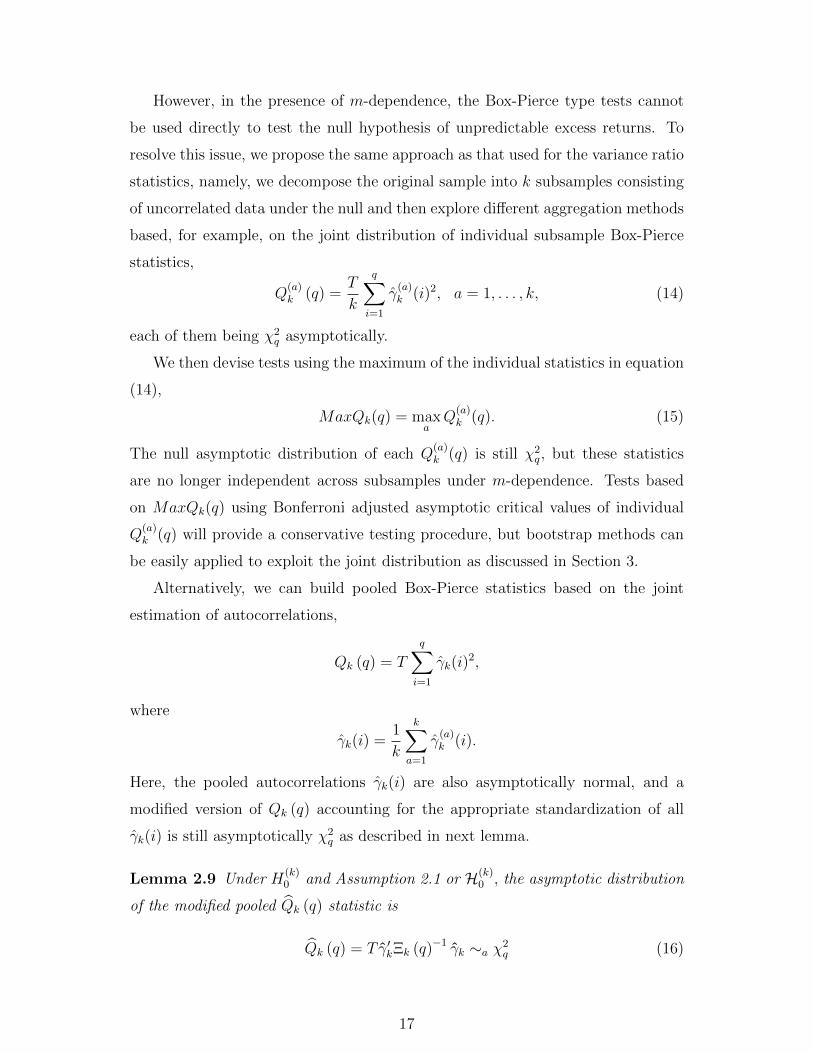
However, in the presence of m-dependence, the Box-Pierce type tests cannot

be used directly to test the null hypothesis of unpredictable excess returns. To

resolve this issue, we propose the same approach as that used for the variance ratio

statistics, namely, we decompose the original sample into k subsamples consisting

of uncorrelated data under the null and then explore different aggregation methods

based, for example, on the joint distribution of individual subsample Box-Pierce

statistics,

Q(a)k (q) =

T

k

q∑i=1

γ(a)k (i)2, a = 1, . . . , k, (14)

each of them being χ2q asymptotically.

We then devise tests using the maximum of the individual statistics in equation

(14),

MaxQk(q) = maxaQ

(a)k (q). (15)

The null asymptotic distribution of each Q(a)k (q) is still χ2

q, but these statistics

are no longer independent across subsamples under m-dependence. Tests based

on MaxQk(q) using Bonferroni adjusted asymptotic critical values of individual

Q(a)k (q) will provide a conservative testing procedure, but bootstrap methods can

be easily applied to exploit the joint distribution as discussed in Section 3.

Alternatively, we can build pooled Box-Pierce statistics based on the joint

estimation of autocorrelations,

Qk (q) = T

q∑i=1

γk(i)2,

where

γk(i) =1

k

k∑a=1

γ(a)k (i).

Here, the pooled autocorrelations γk(i) are also asymptotically normal, and a

modified version of Qk (q) accounting for the appropriate standardization of all

γk(i) is still asymptotically χ2q as described in next lemma.

Lemma 2.9 Under H(k)0 and Assumption 2.1 or H(k)

0 , the asymptotic distribution

of the modified pooled Qk (q) statistic is

Qk (q) = T γ′kΞk (q)−1 γk ∼a χ2q (16)

17

where γk = (γk(1), . . . , γk(q))′ and the elements of Ξk (q) are

Ξ(i,j)k (q) =

1

k2

k∑a=1

k∑b=1

δ(a,b)k (i, j) , i, j = 1, . . . , q,

with δ(a,b)k (i, j) given in equation (5).

To apply this statistic to the cases where conditional heteroscedasticity is al-

lowed, Ξ(i,j)k can be estimated by plugging in the estimates of the asymptotic

covariances δ(a,b)k (i, j) of the sample autocorrelations.

2.6 Discussion

We have focused on applying our aggregation methods across subsamples to

three serial dependence tests. The same idea can also be used for other tests

such as regression and general non-parametric tests. For example, we can employ

our methods to regression (11) or to regression-based predictability tests by imple-

menting the Wald, maximum/minimum, or pooled methods, based on the different

coefficient estimates, such as OLS, Campbell and Yogo (2005), and Jansson and

Moreira (2005).

Furthermore, one can adapt these methods to the sign and signed rank test

by Campbell and Dufour (1995) under m-dependence in a similar way. Camp-

bell and Dufour proposed conditional independence tests with exact finite sample

distribution under the null. These are nonparametric tests based on signs and

ranks that replace observed data and residuals, being valid under general forms of

non-normality and conditional heteroscedasticity. In the presence of m-dependent

disturbances, these tests can only be used directly on subsamples, leading to the

usual aggregation problem.

From a related perspective, the variance ratio statistics using the ranks of

Wright (2000)9 can be especially useful in the presence of data with either outliers

or important non-normality features that can affect the precision of the asymptotic

results or even their validity if higher order moments are not finite. Let rj(ξt|k) be

the rank of ξt|k among all elements ξj|k, ξk+j|k, . . . , ξT−k+j|k in subsample j. Then,

9Wright provides several alternative variance ratio tests using the ranks and signs of a timeseries. In principle, our methods can be applied to all of his tests. For the sake of simplicity, weonly discuss the application of rank-based variance ratio tests.

18

a simple linear transformation of the ranks rj(ξt|k) is defined by

rt =

(rj(ξt|k)−

T/k + 1

2

)((T/k − 1)(T/k + 1)

12

)−1/2,

where rt is standardized with sample mean 0 and variance 1. The rank-based

variance ratio statistic V rj|k(q) = (qgk(q))

−1∑T/kt=q

(rk(t−1)+j + · · ·+ rk(t−q)+j

)2in

subsample j is obtained by simply substituting rt for ξt|k in Vj|k(q). Let

U rk (q) =

√T/k√

2(q − 1)(2q − 1)/3q

(V r1|k(q)− 1, . . . , V r

k|k(q)− 1)′.

The denominator V rj|k(1), corresponding to Vj|k(1) in Uk(q) in equation (4), is

omitted because it is equal to 1 by construction. Then, the rank-based maximum,

minimum, and median variance ratios are calculated by

Maxzrk(q) = maxU rk (q), Minzrk(q) = minU r

k (q), Medzrk(q) = median U rk (q).

(17)

We now relate our results to the long-horizon tests based on the variance ratios.

It is now well established that the finite-sample distribution of variance ratios and

autocorrelation statistics can be quite different from the usual asymptotic approx-

imations due to overlap in the returns data, in particular with a small number of

non-overlapping asset returns. For example, Richardson and Stock (1989) show

that sample variance ratios are not consistent if q/T approaches some constant

and that asymptotic results based on fixed q theory perform poorly in finite sam-

ples. Our sample splitting methods would not solve this problem and should be

limited to cases in which q/(T/k) is reasonably small. To avoid any confusion, we

emphasize that the efficiency gains from our methods are achieved by exploiting

all subsamples for a given value of q/(T/k), which can work well in testing the

expectations hypothesis with relatively small values of q.10 If there is concern

regarding the poor finite sample properties of the conventional variance ratios

bootstrap methods can alternatively be used to alleviate those size distortions in

finite samples. We show that a parametric bootstrap method presented in the next

10Richardson and Stock (1989) assume that asset prices follow a random walk so that theanalysis is limited to k = 1. In this case, increasing T using higher frequency data would notsolve the issue because q will also increase proportionally. See, for example, Campbell, Lo, andMacKinlay (1997, p. 79) for the discussion on this matter. On the other hand, our focus is oncases of k > 1, which is dictated, e.g., by maturity (but not a research choice). So, the useof higher frequency data can obtain power gains by exploiting information from increasing thenumber, k, of subsamples.

19

section obtains quite reasonable size properties even for longer return horizons in

a variety of situations.

We finally discuss some possible power disadvantages of our sample splitting

methods. If higher order dependence only occurs at some specific lags, e.g., over

lag k + 1, the tests based on our methods might not detect this dependence. One

solution to this identification problem is to use sampling at longer intervals such as

k + 1, k + 2, etc., which renders subsamples with independent observations under

the null and spans wider ranges of dependence. These alternative sample splitting

schemes still generate dependence between subsamples, which could be accounted

for using similar methods.

3 Bootstrap Approximations

The asymptotic tests based on variance ratios are liable to have important size

distortions for several reasons. The distribution of variance ratios is asymmetric

because they are bounded by zero from below. The use of large q relative to

sample size T can affect the finite sample properties of estimates of Ωk or Σk. The

maximum deviation tests based on the Bonferroni inequality are very conservative

in some circumstances. The finite sample properties of Box-Pierce and regression-

based tests can also be poorly approximated by the asymptotic distribution in

situations with a small number of non-overlapping excess returns. Therefore, it

is worth pursuing better approximations of the actual joint distribution of those

statistics, which also permit a wider range of tests in applications to be conducted.

We use bootstrap techniques to improve the finite sample performance of those

serial dependence tests that depend on the joint distribution of subsample statistics

and to provide an approximation of the asymptotic distribution of any particular

continuous functional. One possibility in the present context is to use the block

bootstrap method by Kunsch (1989), which allows for the approximation of the

asymptotic distribution of statistics based on a weak dependent time series, such

as m-dependent series under the nonparametric null hypothesis H(k)0 . However,

we instead adopt the parametric bootstrap procedures based on the null H(k)0

under Assumptions 2.1 and 2.2. This approach avoids selecting the order of an

approximating parametric model, such as the autoregressive sieve bootstrap of

Buhlmann (1997), because the dependence horizon is known in our case.

20

To conserve space, we only provide a description of our bootstrap procedure

for the statistics that are continuous functionals of the subsample variance ratios,

VR(j)

k , j = 1, . . . , k, but similar ideas apply to pooled estimates or other statistics

depending on the autocovariances of subsamples.

1. Fit an MA(k − 1) model with an intercept to the original sample S =

ξ1|k, ξ2|k, . . . , ξT |k and obtain residuals et, t = 1, 2, . . . , T setting the ini-

tial values to zero.

2. Obtain an independent resample of size 2T , e∗1, e∗2, . . . , e∗2T from the empiri-

cal distribution of the centered residuals et = et−eT , where eT = T−1∑T

t=1 et.

3. Take the moving averages y∗t of the resampled errors e∗t from step 2 using

the estimated parameter values in step 1 and construct a bootstrap sample

S∗ = ξ∗1 , ξ∗2 , . . . , ξ∗T = y∗T+1, y∗T+2, . . . , y

∗2T.

4. Divide the bootstrap sample into k subsamples, S∗1 = ξ∗1 , ξ∗k+1, . . . , ξ∗T−k+1,

. . ., S∗k = ξ∗k, ξ∗2k, . . . , ξ∗T−k+k. Then, calculate variance ratios√T/k(VR

(j)∗k (q)−

1), j = 1, . . . , k and construct any test statistic of interest from these.

5. Repeat steps 2 to 4 B times.

6. Obtain estimates of the critical values for the one-sided and two-sided tests

based on the empirical distribution of the corresponding bootstrap statistics.

These estimated critical values can be compared to the test statistics obtained

from the data. Note that this bootstrap algorithm simulates the distribution of

variance ratio statistics under the null H(k)0 by imposing a MA(k− 1) structure on

the independent resampled residuals. In step 2, we obtain a sample of size 2T to

eliminate the influence of the initial values, which are set to zero.

The next lemma formally justifies that our bootstrap method can be applied

to the statistics introduced in the previous section when the parameter estimates

of the invertible MA structure are asymptotically equivalent to the maximum like-

lihood estimates, following similar procedures to those in Bose (1990) and Kreiss

and Franke (1992).

Lemma 3.1 Under H(k)0 and Assumption 2.2, and if the roots of the MA(k − 1)

polynomial with ck = 1 are outside the unit circle, c1 6= 0,√T/k(VR

(j)∗k (q) − 1),

21

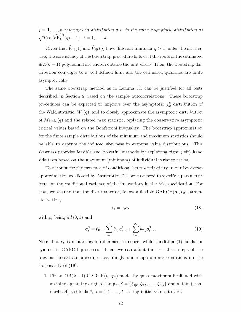
j = 1, . . . , k converges in distribution a.s. to the same asymptotic distribution as√T/k(VR

(j)

k (q)− 1), j = 1, . . . , k.

Given that Vj|k(1) and Vj|k(q) have different limits for q > 1 under the alterna-

tive, the consistency of the bootstrap procedure follows if the roots of the estimated

MA(k − 1) polynomial are chosen outside the unit circle. Then, the bootstrap dis-

tribution converges to a well-defined limit and the estimated quantiles are finite

asymptotically.

The same bootstrap method as in Lemma 3.1 can be justified for all tests

described in Section 2 based on the sample autocorrelations. These bootstrap

procedures can be expected to improve over the asymptotic χ2k distribution of

the Wald statistic, Wk(q), and to closely approximate the asymptotic distribution

of Minzk(q) and the related max statistic, replacing the conservative asymptotic

critical values based on the Bonferroni inequality. The bootstrap approximation

for the finite sample distributions of the minimum and maximum statistics should

be able to capture the induced skewness in extreme value distributions. This

skewness provides feasible and powerful methods by exploiting right (left) hand

side tests based on the maximum (minimum) of individual variance ratios.

To account for the presence of conditional heteroscedasticity in our bootstrap

approximation as allowed by Assumption 2.1, we first need to specify a parametric

form for the conditional variance of the innovations in the MA specification. For

that, we assume that the disturbances et follow a flexible GARCH(p1, p2) param-

eterization,

et = εtσt (18)

with εt being iid (0, 1) and

σ2t = θ0 +

p1∑i=1

θ1,ie2t−i +

p2∑j=1

θ2,jσ2t−j. (19)

Note that et is a martingale difference sequence, while condition (1) holds for

symmetric GARCH processes. Then, we can adapt the first three steps of the

previous bootstrap procedure accordingly under appropriate conditions on the

stationarity of (19).

1. Fit an MA(k− 1)-GARCH(p1, p2) model by quasi maximum likelihood with

an intercept to the original sample S = ξ1|k, ξ2|k, . . . , ξT |k and obtain (stan-

dardized) residuals εt, t = 1, 2, . . . , T setting initial values to zero.

22

2. Obtain an independent resample of size 2T , ε∗1, ε∗2, . . . , ε∗2T, from the empiri-

cal distribution of the centered residuals εt = εt−εT , where εT = T−1∑T

t=1 εt.

3a. Simulate a GARCH(p1, p2) series e∗t of size 2T with parameter values from

the estimates of step 1 and resampled errors ε∗t from step 2 as innovations.

3b. Compute the moving averages y∗t of the simulated heteroscedastic errors e∗t

from step 3a using the estimated parameter values in step 1 and construct a

bootstrap sample S∗ = ξ∗1 , ξ∗2 , . . . , ξ∗T = y∗T+1, y∗T+2, . . . , y

∗2T.

Then, the procedure continues as before in steps 4-6. The justification of the

bootstrap methods for the statistics of GARCH processes under regularity condi-

tions on θ and εt follows from Hidalgo and Zaffaroni (2007) [see also Assumption A

and the discussion in Corradi and Iglesias (2008)], but we omit the details.

4 An Application: Uncovered Interest Parity

We now apply the econometric methods developed in the previous sections to

the tests of uncovered interest rate parity (UIP), that is, the expectations hypoth-

esis in foreign exchange markets. Under the assumptions of rational expectations

and risk-neutral preferences, UIP is defined by

Et[st+k]− st = it|k − i∗t|k, for each maturity k,

where Et[·] denotes the mathematical expectation given the information set avail-

able at time t, st is the log of the spot exchange rate, or the log of the home

currency price of foreign currency at time t, and it|k(i∗t|k) is the nominal interest

rate on home (foreign) deposits with a maturity of k periods. Assuming that

covered interest rate parity holds,

ft|k − st = it|k − i∗t|k, for each maturity k,

where ft|k is the log of the forward exchange rate, or the time t home currency

price of the foreign currency delivered at time t + k. Then, UIP is equivalent to

the unbiasedness hypothesis of forward exchange rates defined by

Et[st+k] = ft|k, for each maturity k. (20)

In this sense, UIP implies that the foreign excess return between t and t + k,

st+k − ft|k, should be unpredictable using any variables in the time t information

23

set. As the definition of the foreign excess return indicates, any predictability tests

need to take into account the (k − 1)-dependence of excess returns, which might

motivate the use of our sample splitting methods.

The alternative hypothesis we are interested in has the following form:

Et[st+k] = ft|k − pt|k, for each maturity k, (21)

where pt|k is a deviation from UIP interpreted as a risk premium or as an expecta-

tional error. In this paper, we mainly consider these two alternatives because they

have been widely used in the literature.11 Furthermore, Moon and Velasco (2011)

argue that these two alternatives in the literature tend to generate the opposite sign

of serial dependence of excess returns, which can be used to judge the performance

of economic models. For example, they show that the rational expectations risk

premium models generate negative serial dependence patterns, while the models

of expectational errors tend to generate positive serial dependence patterns.

As a data-generating process, we use the typical monetary model of exchange

rates.12 In the model, the home money market relationship is given by

lnMt = lnPt + γy lnYt − φkit|k, (22)

where M,P , and Y are the home money supply, the price level, and the output,

respectively. γy is the income elasticity of money demand and φk is the interest

semi-elasticity of money demand, which varies with maturity k. We assume that a

similar equation holds in the foreign country. The corresponding foreign variables

are denoted by asterisks and the parameters of the money demand are the same in

both countries. From (21), covered interest parity, the home money market rela-

tionship (22) and its foreign counterpart, we derive a setup for the determination

of the exchange rate:

st = bEt[st+k] + bpt|k + (1− b)wt + (1− b)$t, (23)

where b = φk1+φk

is the discount factor, wt is the linear combination of the funda-

mental variables, wt = lnMt − lnM∗t − γy(lnYt − lnY ∗t ), and $t is the log of the

11There are other explanations in the literature that are mainly related to small sample prob-lems such as the peso problem, learning, and statistical biases. The variance ratio tests employedin the paper are robust to the statistical biases that typically arise in the regression-based tests.

12See, e.g., Engel and West (2005) and Obstfeld and Rogoff (2002) for the rational expectationsmodels and Frankel and Froot (1990) for the expectational errors models. See also the referencestherein.

24

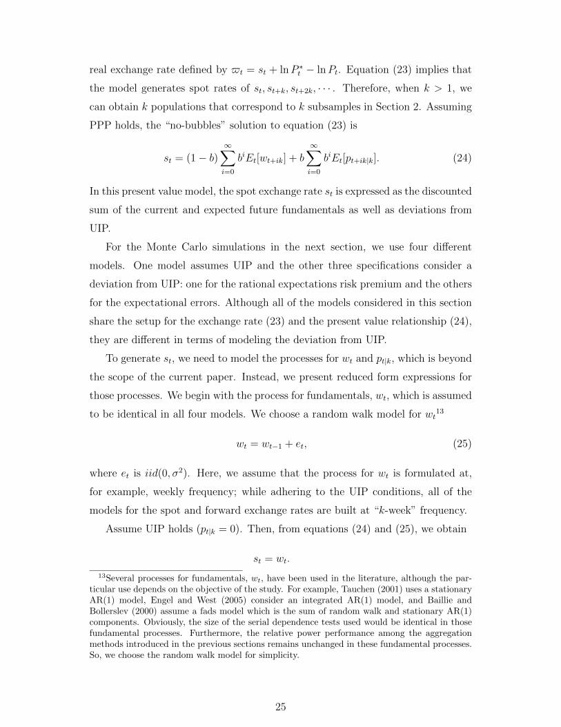
real exchange rate defined by $t = st + lnP ∗t − lnPt. Equation (23) implies that

the model generates spot rates of st, st+k, st+2k, · · · . Therefore, when k > 1, we

can obtain k populations that correspond to k subsamples in Section 2. Assuming

PPP holds, the “no-bubbles” solution to equation (23) is

st = (1− b)∞∑i=0

biEt[wt+ik] + b

∞∑i=0

biEt[pt+ik|k]. (24)

In this present value model, the spot exchange rate st is expressed as the discounted

sum of the current and expected future fundamentals as well as deviations from

UIP.

For the Monte Carlo simulations in the next section, we use four different

models. One model assumes UIP and the other three specifications consider a

deviation from UIP: one for the rational expectations risk premium and the others

for the expectational errors. Although all of the models considered in this section

share the setup for the exchange rate (23) and the present value relationship (24),

they are different in terms of modeling the deviation from UIP.

To generate st, we need to model the processes for wt and pt|k, which is beyond

the scope of the current paper. Instead, we present reduced form expressions for

those processes. We begin with the process for fundamentals, wt, which is assumed

to be identical in all four models. We choose a random walk model for wt13

wt = wt−1 + et, (25)

where et is iid(0, σ2). Here, we assume that the process for wt is formulated at,

for example, weekly frequency; while adhering to the UIP conditions, all of the

models for the spot and forward exchange rates are built at “k-week” frequency.

Assume UIP holds (pt|k = 0). Then, from equations (24) and (25), we obtain

st = wt.

13Several processes for fundamentals, wt, have been used in the literature, although the par-ticular use depends on the objective of the study. For example, Tauchen (2001) uses a stationaryAR(1) model, Engel and West (2005) consider an integrated AR(1) model, and Baillie andBollerslev (2000) assume a fads model which is the sum of random walk and stationary AR(1)components. Obviously, the size of the serial dependence tests used would be identical in thosefundamental processes. Furthermore, the relative power performance among the aggregationmethods introduced in the previous sections remains unchanged in these fundamental processes.So, we choose the random walk model for simplicity.

25

Because equations (20) and (25) imply ft|k = wt, the foreign excess return between

t and t+ k is

st+k − ft|k =k∑j=1

et+i. (26)

We call this result Model 1 in our Monte Carlo simulations in the next section.

We present a risk premium alternative in Model 2. The process for the time

varying risk premium between t and t+ k is given by

pt|k = (1− ϕk)p+ ϕkpt−k|k + νt + · · ·+ νt−k+1, (27)

where 0 < ϕk < 1 and νt is iid(0, σ2ν). The process for the risk premium is modeled

such that it conforms with a maturity k in equation (21). Using equations (24),

(25), and (27), the expression for the spot exchange rate is obtained as

st = wt +b

1− bϕkpt|k, (28)

where the constant terms are omitted for simplicity. Here, the spot exchange rate

is expressed by the sum of a random walk fundamental and a stationary risk pre-

mium, mirroring a well-known fads model for studying the long-run predictability

of stock returns in Fama and French (1988) and Poterba and Summers (1988).

The forward exchange rate is derived from equations (21), (25), (27), and (28)

ft|k = Et[st+k] + pt|k = wt +1

1− bϕkpt|k.

Then, the foreign excess return between t and t+ k under the risk premium alter-

native is

st+k − ft|k =k∑i=1

et+i +b

1− bϕk

k∑i=1

νt+i − pt|k, (29)

where the first two terms in the right-hand side of equation (29) are rational

forecasting errors: et is from the fundamental process and νt is from the risk

premium process. Equation (29) can be viewed as a reduced form expression for

the excess return that is derived from the time-varying risk premium models in

the literature. The expression shows that the forecasting errors will be correlated

with the future values of the risk premium, reflecting a feedback mechanism that

mainly determines the sign of the autocorrelations of excess returns. As shown in

26

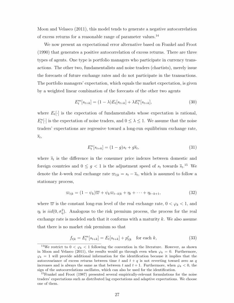
Moon and Velasco (2011), this model tends to generate a negative autocorrelation

of excess returns for a reasonable range of parameter values.14

We now present an expectational error alternative based on Frankel and Froot

(1990) that generates a positive autocorrelation of excess returns. There are three

types of agents. One type is portfolio managers who participate in currency trans-

actions. The other two, fundamentalists and noise traders (chartists), merely issue

the forecasts of future exchange rates and do not participate in the transactions.

The portfolio managers’ expectation, which equals the market expectation, is given

by a weighted linear combination of the forecasts of the other two agents

Emt [st+k] = (1− λ)Et[st+k] + λEn

t [st+k], (30)

where Et[·] is the expectation of fundamentalists whose expectation is rational,

Ent [·] is the expectation of noise traders, and 0 ≤ λ ≤ 1. We assume that the noise

traders’ expectations are regressive toward a long-run equilibrium exchange rate,

st,

Ent [st+k] = (1− g)st + gst, (31)

where st is the difference in the consumer price indexes between domestic and

foreign countries and 0 ≤ g < 1 is the adjustment speed of st towards st.15 We

denote the k-week real exchange rate $t|k = st − st, which is assumed to follow a

stationary process,

$t|k = (1− ψk)$ + ψk$t−k|k + ηt + · · ·+ ηt−k+1, (32)

where $ is the constant long-run level of the real exchange rate, 0 < ϕk < 1, and

ηt is iid(0, σ2η). Analogous to the risk premium process, the process for the real

exchange rate is modeled such that it conforms with a maturity k. We also assume

that there is no market risk premium so that

ft|k = Emt [st+k] = Et[st+k] + pet|k for each k, (33)

14We restrict to 0 < ϕk < 1 following the convention in the literature. However, as shownin Moon and Velasco (2011), the results would go through even when ϕk = 0. Furthermore,ϕk = 1 will provide additional information for the identification because it implies that theautocovariance of excess returns between time t and t + q is not reverting toward zero as qincreases and is always the same as that between t and t + 1. Furthermore, when ϕk < 0, thesign of the autocorrelations oscillates, which can also be used for the identification.

15Frankel and Froot (1987) presented several empirically-relevant formulations for the noisetraders’ expectations such as distributed lag expectations and adaptive expectations. We chooseone of them.

27

where pet|k = Emt [st+k] − Et[st+k] is an expectational error due to the presence of

noise traders and represents a deviation from UIP. Then, analogous to the risk

premium model, we have a setup for determining the exchange rate under the

expectational error alternative using

st = bEt[st+k] + bpet|k + (1− b)wt + (1− b)$t|k.

Note that the main difference from the previous setup under the rational expecta-

tions risk premium is that the risk premium pt|k is replaced by the expectational

error. Using the definition of pet|k and equations (30)-(32), we can rewrite the above

equation as

st = bEt[st+k] + bpet|k + (1− b)wt, (34)

where b = b(1−λ)1−bλ and pet|k = 1−b(1+λg)

b(1−λ) $t|k. The discount factor, b, is now related

not only to the interest semi-elasticity of the money demand but also to the weight

of the noise traders’ expectation, λ, in the market expectation.

Assuming no-bubble solutions, the foreign excess return is derived from equa-

tions (25) and (30)-(34)

st+k − ft|k =k∑i=1

et+i +1− b(1 + λg)

1− bλ− b(1− λ)ψk

k∑i=1

ηt+i − pet|k. (35)

For the sake of simplicity, we relegate the derivation of equation (35) to Appendix

B. We call this Model 3 in the simulations. Analogous to the risk premium alterna-

tive, the forecasting errors are correlated with the future values of pet|k, illustrating

the feedback mechanism. However, the excess returns now exhibit positive auto-

correlations for a reasonable range of parameter values.16

The power pattern of the variance ratio test with q would be quite similar

between the risk premium and the expectational errors alternatives because both

alternatives follow stationary AR(1) processes, although rejections mainly occur

at the opposite tail. That is, the power of the test will initially increase and

then decrease with q [see, e.g., Lo and MacKinlay (1989)]. For comparison, we

consider another alternative that generates a different power pattern with q by

modifying the noise traders’ expectation in equation (31) in the following way:

16Here, we confine our attention to the case where the real exchange rate is mean reverting inthe long run. However, allowing ψk = 1 would only strengthen the result.

28

Ent [st+k] = Et−k[st]. Assuming PPP holds, then the foreign excess return between

t and t+ k is

st+k − ft|k = (1− bλ)k∑i=1

et+i + λ

k−1∑i=0

et−i. (36)

Again, we relegate the derivation to Appendix B. We call this specification Model 4.

As shown in the Monte Carlo experiments, equation (36) generates not only posi-

tive autocorrelations but also a uniformly declining power of the serial dependence

tests with q.

5 Monte Carlo Simulations

We conduct Monte Carlo experiments to study the finite sample properties of

the test statistics for m-dependent data developed in Section 2. We explore the

properties of both asymptotic and parametric bootstrap tests for each statistic.

To improve the numerical efficiency in the simulations of bootstrap asymptotic

size and power, we use the method of Giacomini, Politis and White (2012), where

each simulation generates only one bootstrap resample and a single critical value

is estimated from all of the resamples.

5.1 Econometric Frameworks for Monte Carlo Simulations

To measure the size and power of the test statistics, we use four models pre-

sented in Section 4:

• Model 1 uses equations (25) and (26).

• Model 2 uses equations (25), (27), and (29).

• Model 3 uses equations (25), (32), and (35).

• Model 4 uses equations (25) and (36).

Model 1 generates excess returns under UIP, so the rejection rates provide the

empirical size of the test statistics. The remaining models generate excess returns,

which exhibit either negative or positive serial dependence. The rejection rates

from these models measure the power of the tests. Model 2 generates a negative

serial dependence of excess returns, while Model 3 and Model 4 generate a positive

serial dependence but with different power patterns over the aggregation value q.

29

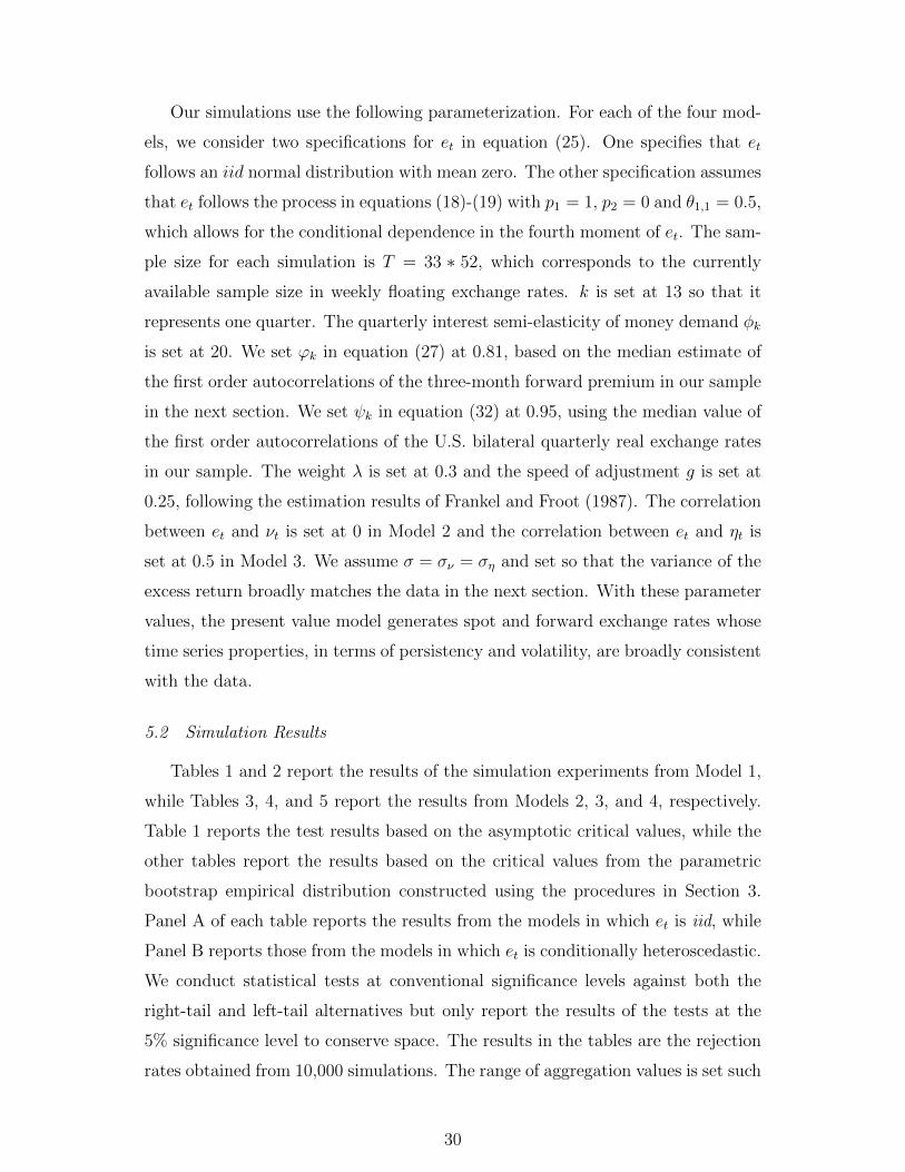
Our simulations use the following parameterization. For each of the four mod-

els, we consider two specifications for et in equation (25). One specifies that et

follows an iid normal distribution with mean zero. The other specification assumes

that et follows the process in equations (18)-(19) with p1 = 1, p2 = 0 and θ1,1 = 0.5,

which allows for the conditional dependence in the fourth moment of et. The sam-

ple size for each simulation is T = 33 ∗ 52, which corresponds to the currently

available sample size in weekly floating exchange rates. k is set at 13 so that it

represents one quarter. The quarterly interest semi-elasticity of money demand φk

is set at 20. We set ϕk in equation (27) at 0.81, based on the median estimate of

the first order autocorrelations of the three-month forward premium in our sample

in the next section. We set ψk in equation (32) at 0.95, using the median value of

the first order autocorrelations of the U.S. bilateral quarterly real exchange rates

in our sample. The weight λ is set at 0.3 and the speed of adjustment g is set at

0.25, following the estimation results of Frankel and Froot (1987). The correlation

between et and νt is set at 0 in Model 2 and the correlation between et and ηt is

set at 0.5 in Model 3. We assume σ = σν = ση and set so that the variance of the

excess return broadly matches the data in the next section. With these parameter

values, the present value model generates spot and forward exchange rates whose

time series properties, in terms of persistency and volatility, are broadly consistent

with the data.

5.2 Simulation Results

Tables 1 and 2 report the results of the simulation experiments from Model 1,

while Tables 3, 4, and 5 report the results from Models 2, 3, and 4, respectively.

Table 1 reports the test results based on the asymptotic critical values, while the

other tables report the results based on the critical values from the parametric

bootstrap empirical distribution constructed using the procedures in Section 3.

Panel A of each table reports the results from the models in which et is iid, while

Panel B reports those from the models in which et is conditionally heteroscedastic.

We conduct statistical tests at conventional significance levels against both the

right-tail and left-tail alternatives but only report the results of the tests at the

5% significance level to conserve space. The results in the tables are the rejection

rates obtained from 10,000 simulations. The range of aggregation values is set such

30

that the maximum value of q is 10 years relative to a base period of a quarter and

includes 2, 4, 8, 12, 16, 20, 32, and 40 quarters. For comparison, we also set n = q,

the holding period horizon in the Fama-French regression, except that q = 2 is

replaced with n = 1.

5.2.1 Size

(Insert Table 1 about here)

Panel A in Table 1 reports the rejection rates of the serial dependence tests

based on asymptotic critical values for the iid excess returns. We use three types of

serial dependence tests: variance ratio, Box-Pierce portmanteau, and Fama-French

regression tests. For the variance ratio tests, we use several aggregates based on

the pooled method, Bonferroni bounds, and the Wald method. Overall, most tests

have a reasonable size at the right-tail for the smaller aggregation value q, while

the variance ratio tests under-reject at the left-tail.

We begin with the test results at the right-tail. The empirical sizes of the

t-statistic of pooled variance ratios, zk(q), appear to be reasonable at the-right tail

over all q considered, although the test slightly over-rejects for large q. For exam-

ple, the rejection rates associated with the aggregation values q = 2, 4, 8, 12, 16, 20, 32,

and 40 quarters, are 4, 5, 6, 7, 7, 7, 8, and 9% at the right-tail, respectively. The

size of the Bonferroni maximum variance ratio test is close to the nominal value

even for large q: its rejection rates are approximately 5% for q = 32 and 40. The

right-tail t-test from the Fama-French regression also has a reasonable size over all

q, while the Box-Pierce pooled statistic tends to slightly over-reject for large q.

However, the empirical sizes of the t-statistics of the pooled variance ratios

become distorted for large q at the left-tail. For example, the rejection rates of the

left-tail test are 2% and 1% for q = 32 and q = 40 quarters, respectively. Similarly,

the Bonferroni minimum variance ratio test appears not to reject at all over most

values of q. As in Richardson and Stock (1991), one possible reason for this size

distortion can be that the variance ratios become inconsistent for large q relative

to the sample size T .

Panel B in Table 1 reports the rejection rates of the serial dependence tests in

the presence of conditional heteroscedasticity in excess returns. All of the tests

produce quite similar rejection patterns to those in Panel A.

31

Table 2 reports the rejection rates of the serial dependence tests based on the

critical values obtained from the parametric bootstrap method. In contrast to the

asymptotic tests, there are no size distortions at both tails even for large q. The

empirical sizes of all the tests are close to their nominal value at both tails and for

all q considered. For example, the rejections rates of the t statistics of estimated

pooled variance ratios are all 5% at both tails for each aggregation value q. The

results are almost identical even in the presence of conditional heteroscedasticity.

From now on, we will focus on the results from the parametric bootstrap

method because it corrects the potential size distortions of the serial dependence

tests from both skewness and Bonferroni inequality. Furthermore, we will mainly

discuss the results from the models with iid et because the tests produce similar

size and power properties for both specifications of et.17


5.2.2 Power

We now discuss the power properties of the serial dependence tests. In gen-

eral, the power of the tests is sensitive to the parameterization of the simulated

models. However, the two important features that we are interested in, the sign

of the autocorrelations of the excess returns and the power pattern over q, are not

sensitive for a broad range of parameter values. Nor is the relative performance

over tests considered. Therefore, we do not provide further sensitivity analysis on

the power of the tests with respect to changes in the parameter values.

Negative Serial Dependence


Table 3 reports the results of the serial dependence tests from Model 2. The

rejections mainly occur at the left-tail and the simulated variance ratios are less

than 1, suggesting that the excess returns generated from Model 2 exhibit negative

autocorrelations. Furthermore, the tests produce a hump-shaped power pattern

over q: the rejection rates initially increase and then decrease with q. For example,

17We also conduct the rank-based variance ratio tests because their size and power propertiesare not known for the m-dependent time series data, although their size is exact in finite samplesfor the 0-dependence data as in Wright (2000). We find that all three aggregates of rank-basedvariance ratios such as the minimum, maximum, and median have the size close to the nominalvalue. These results are available upon request.

32

the rejection rates of a pooled variance ratio test associated with the aggregation

values q = 2, 4, 8, 12, 16, 20, 32, and 40 quarters, are 30, 44, 58, 67, 70, 70, 65,

and 60% at the left-tail, respectively. The presence of the strongly persistent

component (the risk premium) in the exchange rates generated from Model 2

explains this non-monotonic power pattern of the variance ratio tests consistent

with Lo and MacKinlay (1989), who show that a mean reverting component in

asset prices generates this nonmonotone power pattern.

We compare the power of three serial dependence tests. The variance ratio

tests, except for the Wald method, are more powerful than the Box-Pierce and

Fama-French regression tests in that the power of the former is greater than those

of the latter for each q. Furthermore, the maximum power of the former is much

greater than the latter. For example, the largest rejection rate of the variance ratio

tests over q is approximately 70%, while those of the Box-Pierce portmanteau and

Fama-French t-tests are approximately 29% and 45%, respectively. The variance

ratio tests based on the pooled, median, maximum, and minimum methods have

similar power properties in terms of rejection rates and power patterns, while the

Wald method performs much worse, with much less power for each aggregation

value q. For example, the rejection rates of the Wald variance test associated with

the aggregation values are all under 3%.

Positive Serial Dependence


Table 4 reports the results from Model 3. Here, the rejections mainly occur at

the right-tail and the simulated variance ratios are greater than one, suggesting

that the excess returns generated from Model 3 display positive autocorrelations.

Furthermore, the power of the tests initially increases and then decreases with q.

This non-monotonic power pattern is produced because the expectational error is

persistent in Model 3, like the risk premium in Model 2.

Similar to Model 2, the variance ratio tests, except for the Wald method, are

more powerful than the Box-Pierce and Fama-French regression tests. For example,

the maximum power of the variance ratio tests is approximately 47%, while those

of the Box-Pierce portmanteau and Fama-French t-tests are approximately 18%

and 36%, respectively. Again, the variance ratio tests based on the pooled, median,

33

maximum, and minimum methods have similar power properties.

Table 5 reports the results from Model 4 which also generates the positive

autocorrelations of excess returns but a different power pattern from Model 3. All

of the serial dependence tests reject the null most strongly when q = 2 and then

their power uniformly decreases with q. For example, the rejection rates of the

pooled variance ratio test associated with the aggregation values are 100, 87, 50,

34, 26, 22, 14, and 13% at the right-tail. These results suggest that not only the

sign of serial dependence but also the power pattern over q can be used to identify

a particular economic alternative.

In contrast to Model 2 and Model 3, the Box-Pierce tests are now more pow-

erful than the variance ratio and Fama-French regression tests. Furthermore, the

power of the former is decreasing relatively more slowly over q. For example, the

rejection rates of the Box-Pierce maximum statistic, MaxQk, associated with the

aggregation values are 99, 99, 92, 84, 77, 71, 60, and 55% at the right-tail, while

the rejection rate of the Fama-French test is already approximately 10% for q=4.


6 Tests for the Expectations Hypothesis in Foreign ExchangeMarkets

In this section, we use our serial dependence tests for testing the predictability

of three-month foreign excess returns from January 1975 to December 2007 using

1716 weekly observations.18 The log foreign excess returns st+k−ft|k are measured

over a holding period of k = 13 weeks and annualized by (st+k−ft|k)∗5200/k. Our

sample includes weekly spot prices of the U.S. dollar against the German mark,

the British pound, and the Japanese yen as well as three-month prices (forward

exchange rates) of the U.S. dollar. The data are simultaneously collected from

London close bid and ask prices and obtained from Global Insight. The mid prices

are used for the empirical study. These are major currencies in foreign exchange

markets and have been widely used for testing UIP, the expectations hypothesis

in foreign exchange markets.


Table 6 reports the p-values of the test statistics obtained from the parametric

18Wednesday’s closing price is selected to form our sample. If the following Wednesday ismissing, then Thursday’s price is used (or Tuesday’s if Thursday’s is missing).

34

empirical bootstrap distributions. The table also reports the pooled variance ra-

tios, VRk(q), defined in equation (9).19 Overall, the expectations hypothesis in the

foreign exchange markets is rejected for the three-month excess returns, confirming

the previous empirical evidence on the predictability of foreign excess returns. In

addition, the patterns of variance ratios over the aggregation values suggest that

the foreign excess returns exhibit positive autocorrelations.

The variance ratio tests reject the expectations hypothesis at the 5% level

against the right-tail alternative up to the aggregation values q = 12 to 16 quarters

relative to a three-month base period. Furthermore, the p-values initially decrease

and then increase or they tend to be almost zero up to a certain q and then start

to increase. For example, the right-tail p-values of the minimum variance ratio

test associated with aggregation values q =2, 4, 8, 12, 16, 20, 32, and 40 quarters

are 2, 0, 0, 0, 0, 1, 8, and 12% for the three-month German mark excess return

against the U.S. dollar.

As predicted from our Monte Carlo simulations, the Fama-French regression

test is not able to reject the null for most values of q. On the other hand, the

Box-Pierce pooled and maximum Q statistics reject the null for the British pound

and Japanese yen excess returns. The p-values of these statistics tend to decrease

and then to increase over q. These results further confirm the conclusions from

the variance ratio tests.

7 Concluding Remarks

This paper investigates both the asymptotic and the finite sample properties

of the serial dependence tests for m-dependent data. We propose a general econo-

metric framework that first splits the original sample into m + 1 subsamples and

then aggregates information across them. These aggregation methods include the

pooled, median, maximum, minimum, and Wald methods. Our Monte Carlo sim-

ulations show that all of these methods except for the Wald perform similarly in

terms of size and power.

Using these methods, we conduct tests for the expectations hypothesis in for-

eign exchange markets and confirm the empirical evidence from previous studies.

In addition, we show that the serial dependence tests further provide informa-

19The variance ratios are slightly different among the aggregation methods. For brevity, weonly report the pooled variance ratios.

35

tion regarding the rejections of the null hypothesis. Evidence on positive serial

dependence of foreign excess returns supports an expectational error alternative.

36

Appendix A. Proofs

Proof of Lemma 2.2. The central limit theorem for Uk (q) follows by the Cramer-

Wold device and by a standard central limit for m-dependent processes, e.g. Di-

ananda (1955), since linear combinations of the cross products involved in autoco-

variances for different subsamples are also finite dependent for fixed lags. For the

asymptotic variance calculation, consider VR(a)

k (q) = 1+2∑q−1

i=1

(1− i

q

)γ(a)k (i)/σ2

k

with γ(a)k (i) being the lag i sample autocovariance of ξt = ξt|k − αk in subsam-

ple a which centers ξt|k around the true mean αk. Then, both VR(a)

k (q) − 1 and

VR(a)

k (q) − 1 have the same asymptotic distribution since γ(a)k (0) →p σ

2k for all

a = 1, . . . , k and αk = αk + Op

(T−1/2

)under the null. Therefore, from direct

calculation from the definition of VR(a)

k (q) − 1, it holds under the null that, for

1 ≤ b ≤ a ≤ k,

2(q − 1)(2q − 1)σ4k

12qΣk(q)

[a,b]

=

q−1∑i=1

(1− i

q

)2

δ(a,b)k (i, i) +

q−1∑i=1

∑j 6=i

(1− i

q

)(1− j

q

)δ(a,b)k (i, j) , (37)

where δ(a,b)k (i, j) is the asymptotic covariance between γ

(a)k (i) and γ

(b)k (j), i, j > 0,

normalized by (T/k)1/2 , given by (5) for j = i±1, while δ(a,b)k (i, j) = 0 for |j−i| > 1

and a 6= b because in this case the collectionξtk, ξrk+a−b, ξ(t+i)k, ξ(t+j)k+a−b

al-

ways contains one (zero mean) component independent of the other three ones

for any t, r = 1, . . . , T/k, and a, b = 1, . . . , k. Similarly δ(a,a)k (i, j) = 0 for i 6= j,

becauseξtk, ξrk, ξ(t+i)k, ξ(t+j)k

always contains independent individual ξt.

Proof of Corollary 2.3. It follows as Lemma 2.2 using Theorem 3 in Lo and

MacKinlay (1988) to exploit condition (1) for obtaining the asymptotic variance

of autocovariances Σk(q).

Proof of Corollary 2.4. Under H(k)0 and Assumption 2.2, using the iid assump-

tion on the innovations of the MA(k − 1) model,

E[ξtξt+a−bξt+ikξt+ik+a−b

]= E

[ξtξt+a−b

]E[ξt+ikξt+ik+a−b

]= E

[ξ0ξa−b

]2E[ξtξt+a−b−kξt+ikξt+a−b−k+ik

]= E

[ξtξt+a−b−k

]E[ξt+ikξt+a−b−k+ik

]= E

[ξ0ξk−a+b

]2E[ξtξt+a−b−kξt+ikξt+ik+a−b

]= E

[ξtξt+a−b−k

]E[ξtξt+a−b

]= E

[ξ0ξk−a+b

]E[ξ0ξa−b

]37

for i ≥ 1, while for i ≥ 2,

E[ξtξt+a−bξt+ikξt+ik+a−b−k

]= E

[ξtξt+a−b

]E[ξt+ikξt+ik+a−b−k

]= E

[ξ0ξa−b

]E[ξ0ξk−a+b

],

by (k − 1)-dependence, where the pairwise expectations of ξt do not depend on i

by stationarity. Note that for i = 1, the first expectation can be calculated as

E[ξtξt+a−bξt+kξt+k+a−b

]= E

[ξtξt+a−b

]E[ξt+kξt+k+a−b

]+ E

[ξtξt+k+a−b

]E[ξt+a−bξt+k

]+ E

[ξtξt+k

]E[ξt+a−bξt+k+a−b

]+ κ

[ξt, ξt+a−b, ξt+k, ξt+k+a−b

],

where κ indicates joint cumulant. Now E[ξtξt+a−b

]E[ξt+kξt+k+a−b

]= E

[ξ0ξa−b

]2,

but E[ξtξt+k+a−b

]= E

[ξtξt+k

]= 0, so the second and third terms are zero. Fi-

nally the joint cumulant is also zero because it can be written as a (weighted) sum

of joint cumulants of the serially independent innovations et. Note that all indexes

of et cannot be the same because ξt and ξt+k+a−b are independent.

A similar analysis can be done for a < b, so that δ(a,b)k (i, i− 1) = δ

(b,a)k (j, j + 1) , i >

1, j > 0, only depends on |a− b|.Then, the result follows by simple algebra noting that (37) is equal to

δ(a,b)k (i, i)

q−1∑i=1

(1− i

q

)2

+ 2δ(a,b)k (i, i− 1)

q−1∑i=2

(1− i

q

)(1− i− 1

q

),

because δ(a,b)k does not depend on i, q2

∑q−1i=1

(1− i

q

)2= (q − 1) q (2q − 1) /6 for

q > 1, and q2∑q−1

i=2

(1− i

q

)(1− i−1

q

)= (q − 1) q (2q − 4) /6 for q > 2. Finally,

for s > 0,

E[ξ0ξs

]2=

k∑i=1

k∑j=1

cicjE (ei−kes+j−k) = σ2

k−s∑i=1

cici−s,

since the expectation is only different from zero for j = i − s, and the sum is

zero when k − s < 1, i.e. s ≥ k. The fact that Σk(q) is positive definite fol-

lows from stationarity and the non perfect correlation among subsamples under

m-dependence.

Proof of Lemma 2.5. It follows from direct calculation from Lemma 2.2, where

i = a − b > 0, and noting that the asymptotic variance of√T VRk(q) is equal

to that of 1k

∑kj=1

√T VR

(j)

k (q) because it is not affected by standardization using

different, but consistent, estimates of σ2k. Then, Λk (q) > 0 follows from Σk(q) > 0,

38

cf. Lemma 2.2, and Bartlett’s weights (k − i) /k in the definition of Λk (q) .

Proof of Corollary 2.6. It follows from Lemma 2.5 and Corollary 2.3.

Proof of Corollary 2.7. It follows from Lemma 2.5 and Corollary 2.4.

Proof of Lemma 2.9. The proof is similar to that of Lemmas 2.2 and 2.5, noting

that γk is asymptotically normal and using directly the variance structure of γ(a)k (i)

to derive Ξ(i,j)k (q).

Proof of Lemma 3.1. We show that the bootstrap versions of VR statistics have

the same asymptotic distribution conditional on the sample, as the original VR

statistics. Since the bootstrapped residuals e∗t are iid conditional on the sample,

and the estimates ci of ci are a.s. consistent under H(k)0 and Assumption 2.2, see

Yao and Brockwell (2006), the bootstrapped ξ∗t follow an MA(k−1) model (up to a

negligible initial condition, see e.g. equation (2.1) in Bose (1990)). Then, to apply

a central limit theorem to VR(j)∗k (q), j = 1, . . . , k, or to any finite collection of sub-

sample autocovariances built with this particular (k − 1)-dependent series, we only

need to check the moment condition E∗ [ξ∗4t ] = O (1) a.s., where E∗ denotes expec-

tation conditional on the sample. For that we note that E∗[(ξ∗t )

4] = E∗[(y∗T+t

)4],

where

ξ∗t = y∗T+t =k∑i=1

cie∗T+t+i−k,

and ck = 1 for identification. Then, we have that

E∗[ξ∗4t]

=k∑

i1=1

· · ·k∑

i4=1

ci1 · · · ci4E∗[e∗T+t+i1−k · · · e

∗T+t+i4−k

],

and E∗[e∗T+t+i1−k · · · e

∗T+t+i4−k

]≤ E∗

[(e∗t )

4] = T−1∑T

t=1 e4t , with et = et − eT .

Finally,

et = ξt −t−1∑i=1

βiξt−i,

where βi are the coefficients of β (L) = 1/(1 + ck−1L+ · · ·+ c1L

k−1) . For large T,

|βi| ≤ Cδik a.s. for some 0 < δk < 1. Then, T−1∑T

t=1 (et)4 → E [e4t ] <∞ a.s., and

the moment condition holds. The covariance structure of subsample bootstrap

39

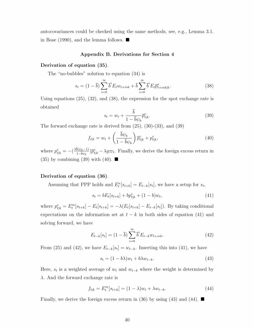
autocovariances could be checked using the same methods, see, e.g., Lemma 3.1.

in Bose (1990), and the lemma follows.

Appendix B. Derivations for Section 4

Derivation of equation (35).

The “no-bubbles” solution to equation (34) is

st = (1− b)∞∑i=0

biEtwt+i∗k + b

∞∑i=0

biEtp

et+i∗k|k. (38)

Using equations (25), (32), and (38), the expression for the spot exchange rate is

obtained

st = wt +b

1− bψkpet|k. (39)

The forward exchange rate is derived from (25), (30)-(33), and (39)

ft|k = wt +

(bψk

1− bψk

)pet|k + pet|k, (40)

where pet|k = −(λb(ψk−1)1−bψk

)pet|k−λg$t. Finally, we derive the foreign excess return in

(35) by combining (39) with (40).

Derivation of equation (36).

Assuming that PPP holds and Ent [st+k] = Et−k[st], we have a setup for st,

st = bEt[st+k] + bpet|k + (1− b)wt, (41)

where pet|k = Emt [st+k]− Et[st+k] = −λ(Et[st+k]− Et−k[st]). By taking conditional

expectations on the information set at t − k in both sides of equation (41) and

solving forward, we have

Et−k[st] = (1− b)∞∑i=0

biEt−kwt+i∗k. (42)

From (25) and (42), we have Et−k[st] = wt−k. Inserting this into (41), we have

st = (1− bλ)wt + bλwt−k. (43)

Here, st is a weighted average of wt and wt−k where the weight is determined by

λ. And the forward exchange rate is

ft|k = Emt [st+k] = (1− λ)wt + λwt−k. (44)

Finally, we derive the foreign excess return in (36) by using (43) and (44).

40

References

Baillie, R., Bollerslev, T., 2000, The forward premium anomaly is not as bad asyou think. Journal of International Money and Finance 19, 471-488.

Bose, A., 1990, Bootstrap in moving average models. Annals of the Institute ofStatistical Mathematics 42, 753-768.

Box, G., Pierce, D., 1970, Distribution of residual autocorrelations in autoregressive-integrated moving average time series models. Journal of the American.Statistical Association 65, 1509-1526.

Buhlmann, P., 1997, Sieve bootstrap for time series. Bernoulli 3, 123-148.

Campbell, B., Dufour, J., 1995, Exact nonparametric orthogonality and randomwalk tests. The Review of Economics and Statistics 77, 1-16.

Campbell, J., Shiller, R., 1991, Yield spreads and interest rate movements: Abird’s eye view. Review of Economic Studies 58, 495-514.

Campbell, J., Yogo, M., 2006, Efficient tests of stock return predictability. Jour-nal of Financial Economics 81, 27-60.

Cochrane, J., 1988, How big is the random walk in GNP?. Journal of PoliticalEconomy 96, 893-920.

Cochrane, J., Piazzesi, M., 2005, Bond risk premia. American Economic Review95, 138-160.

Corradi, V., Iglesias, E., 2008, Bootstrap refinements for QML estimators of theGARCH(1,1) parameters. Journal of Econometrics 144, 500-510.

Delgado, M., Velasco, C. 2011, An asymptotically pivotal transform of the resid-uals sample autocorrelations with application to model checking. Journal ofAmerican Statistical Association, in press.

Diananda, P., 1955, The central limit theorem for m-dependent variables. Math-ematical Proceedings of the Cambridge Philosophical Society 51, 92-95.

Dufour, J., Torres. O., 1998, Union-intersection and sample-split methods ineconometrics with applications to SURE and MA models. Chapter 14 inHandbook of Applied Economic Statistics, Eds. D. Giles and A. Ullah.(Marcel Dekker, New York).

Engel, C., 1996, The forward discount anomaly and the risk premium: A surveyof recent evidence. Journal of Empirical Finance 3, 123-192.

Engel, C., West, K., 2005, Exchange rates and fundamentals. Journal of PoliticalEconomy 113, 485-517.

Escanciano, J., Velasco, C., 2006, Generalized spectral tests for the martingaledifference hypothesis. Journal of Econometrics 134, 151-185.

41

Fama, E., French, K., 1988, Permanent and temporary components of stockprices. Journal of Political Economy 96, 246-273.

Frankel, J., Froot, K., 1987, Using survey data to test standard propositionsregarding exchange rate expectations. American Economic Review 77, 133-153.

Frankel, J., Froot, K., 1990, Chartists, fundamentalists, and demand for dollars.In Anthony S. Courakis and Mark P. Taylor, ed.: Private Behavior andInterdependent Government Policy (Clarendon Press, Oxford).

Giacomini, R., Politis, N., White, H., 2012, A Warp-speed method for conductingMonte Carlo experiments involving bootstrap estimators. mimeo.

Godfrey, L., 1978, Testing against general autoregressive and moving average er-ror models when the regressors include lagged dependent variables. Econo-metrica 46, 1293-1301.

Hansen, L., Hodrick, R., 1980, Forward exchange rates as optimal predictors offuture spot rates: An econometric analysis. Journal of Political Economy88, 829-53.

Hidalgo, J., Zaffaroni, P., 2007, A goodness-of-fit test for ARCH(∞) model. Jour-nal of Econometrics 141, 835-875.

Jansson, M., Moreira, M., 2006, Optimal inference in regression models withnearly integrated regressors. Econometrica 74, 681-714.

Kreiss, J-P., Franke, J., 1992, Bootstrapping stationary autoregressive moving-average models. Journal of Time Series Analysis 13, 297-321.

Kunsch, H., 1989, The jackknife and the bootstrap for general stationary obser-vations. Annals of Statistics 17 , 1217-1241.

Lewis, K., 1995, Puzzles in international financial markets. in Gene Grossmanand Kenneth Rogoff (eds.), Handbook of International Economics 3, Ams-terdam: North Holland.

Liu, C. He, J., 1991, A variance-ratio test of random walks in foreign exchangerates. Journal of Finance 46, 773-785.

Ljung, G., Box, G., 1978, On a measure of a lack of fit in time series models.Biometrika 65, 297-303.

Lo, A., MacKinlay, C., 1988, Stock market prices do not follow random walks:Evidence from a simple specification test. Review of Financial Studies 1,41-66.

Lo, A., MacKinlay, C., 1989, The size and power of the variance ratio tests infinite samples: A monte carlo investigation. Journal of Econometrics 40 ,203-38.

42

Moon, S., Velasco, C., 2011, The forward discount puzzle: identification of eco-nomic assumptions. Universidad Carlos III de Madrid.

Newey, W., West, K., 1987, A simple, positive semi-definite, heteroscedasticityand autocorrelation consistent covariance matrix. Econometrica 55, 703-708.

Obstfeld, M., Rogoff, K., 2002, Risk and exchange rates. in Elhanan Helpmanand Effraim Sadka (eds.), Contemporary Economic Policy: Essays in Honorof Assaf Razin. Cambridge: Cambridge University Press.

Poterba, J., Summers, L., 1988, Mean reversion in stock prices: evidence andimplications. Journal of Financial Economics 22, 27-59.

Richardson, M., Smith, T., 1991, Tests of financial models in the presence ofoverlapping observations. The Review of Financial Studies 4, 227-254.

Richardson, M., Stock, J., 1989, Drawing inferences from statistics based onmultiyear asset returns. Journal of Financial Economics 25, 323-348.

Tauchen, G., 2001, The bias of tests for a risk premium in forward exchange rates.Journal of Empirical Finance 8, 695-704.

Wright, J., 2000, Alternative variance ratio tests using ranks and signs. Journalof Business and Economic Statistics 18, 1-9.

Yao, Q., Brockwell, P. 2006, Gaussian maximum likelihood estimation for ARMAmodels I. Time Series. Journal of Times Series Analysis 27, 857-875.

43

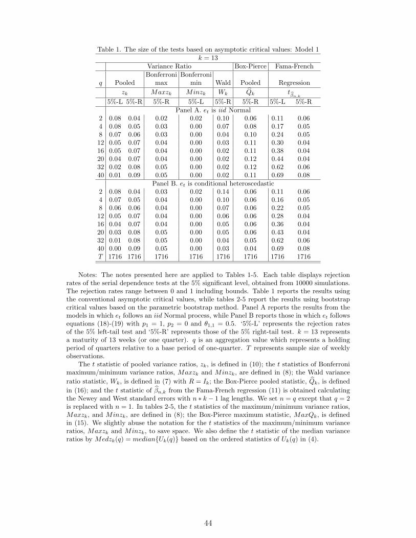
Table 1. The size of the tests based on asymptotic critical values: Model 1k = 13

Variance Ratio Box-Pierce Fama-FrenchBonferroni Bonferroni

q Pooled max min Wald Pooled Regression

zk Maxzk Minzk Wk Qk tβn,k

5%-L 5%-R 5%-R 5%-L 5%-R 5%-R 5%-L 5%-RPanel A. et is iid Normal

2 0.08 0.04 0.02 0.02 0.10 0.06 0.11 0.064 0.08 0.05 0.03 0.00 0.07 0.08 0.17 0.058 0.07 0.06 0.03 0.00 0.04 0.10 0.24 0.0512 0.05 0.07 0.04 0.00 0.03 0.11 0.30 0.0416 0.05 0.07 0.04 0.00 0.02 0.11 0.38 0.0420 0.04 0.07 0.04 0.00 0.02 0.12 0.44 0.0432 0.02 0.08 0.05 0.00 0.02 0.12 0.62 0.0640 0.01 0.09 0.05 0.00 0.02 0.11 0.69 0.08

Panel B. et is conditional heteroscedastic2 0.08 0.04 0.03 0.02 0.14 0.06 0.11 0.064 0.07 0.05 0.04 0.00 0.10 0.06 0.16 0.058 0.06 0.06 0.04 0.00 0.07 0.06 0.22 0.0512 0.05 0.07 0.04 0.00 0.06 0.06 0.28 0.0416 0.04 0.07 0.04 0.00 0.05 0.06 0.36 0.0420 0.03 0.08 0.05 0.00 0.05 0.06 0.43 0.0432 0.01 0.08 0.05 0.00 0.04 0.05 0.62 0.0640 0.00 0.09 0.05 0.00 0.03 0.04 0.69 0.08T 1716 1716 1716 1716 1716 1716 1716 1716

Notes: The notes presented here are applied to Tables 1-5. Each table displays rejectionrates of the serial dependence tests at the 5% significant level, obtained from 10000 simulations.The rejection rates range between 0 and 1 including bounds. Table 1 reports the results usingthe conventional asymptotic critical values, while tables 2-5 report the results using bootstrapcritical values based on the parametric bootstrap method. Panel A reports the results from themodels in which et follows an iid Normal process, while Panel B reports those in which et followsequations (18)-(19) with p1 = 1, p2 = 0 and θ1,1 = 0.5. ‘5%-L’ represents the rejection ratesof the 5% left-tail test and ‘5%-R’ represents those of the 5% right-tail test. k = 13 representsa maturity of 13 weeks (or one quarter). q is an aggregation value which represents a holdingperiod of quarters relative to a base period of one-quarter. T represents sample size of weeklyobservations.

The t statistic of pooled variance ratios, zk, is defined in (10); the t statistics of Bonferronimaximum/minimum variance ratios, Maxzk and Minzk, are defined in (8); the Wald variance

ratio statistic, Wk, is defined in (7) with R = Ik; the Box-Pierce pooled statistic, Qk, is defined

in (16); and the t statistic of βn,k from the Fama-French regression (11) is obtained calculatingthe Newey and West standard errors with n ∗ k − 1 lag lengths. We set n = q except that q = 2is replaced with n = 1. In tables 2-5, the t statistics of the maximum/minimum variance ratios,Maxzk, and Minzk, are defined in (8); the Box-Pierce maximum statistic, MaxQk, is definedin (15). We slightly abuse the notation for the t statistics of the maximum/minimum varianceratios, Maxzk and Minzk, to save space. We also define the t statistic of the median varianceratios by Medzk(q) = medianUk(q) based on the ordered statistics of Uk(q) in (4).

44

Table 2. The size of the tests based on the parametric bootstrap method: Model 1k = 13

Variance Ratio Box-Pierce Fama-Frenchq pooled median max min Wald pooled max regression

zk Medzk Maxzk Minzk Wk Qk MaxQk tβn,k

5%-L 5%-R 5%-L 5%-R 5%-L 5%-R 5%-L 5%-R 5%-R 5%-R 5%-R 5%-L 5%-RPanel A. et is iid Normal

2 0.05 0.05 0.05 0.06 0.05 0.05 0.05 0.05 0.05 0.05 0.05 0.05 0.054 0.05 0.05 0.05 0.05 0.05 0.05 0.05 0.05 0.05 0.05 0.05 0.05 0.058 0.05 0.05 0.05 0.05 0.05 0.05 0.05 0.05 0.05 0.05 0.05 0.05 0.0512 0.06 0.05 0.06 0.05 0.06 0.05 0.05 0.05 0.05 0.04 0.05 0.05 0.0516 0.05 0.05 0.05 0.05 0.05 0.05 0.05 0.05 0.04 0.05 0.05 0.05 0.0520 0.05 0.05 0.05 0.05 0.05 0.05 0.05 0.05 0.04 0.05 0.05 0.05 0.0632 0.05 0.05 0.05 0.05 0.05 0.04 0.05 0.05 0.04 0.05 0.05 0.05 0.0640 0.05 0.05 0.05 0.05 0.05 0.04 0.04 0.05 0.04 0.05 0.05 0.05 0.05

Panel B. et is conditional heteroscedastic2 0.05 0.05 0.06 0.05 0.06 0.04 0.05 0.05 0.05 0.06 0.05 0.05 0.054 0.05 0.05 0.06 0.05 0.05 0.04 0.05 0.05 0.05 0.05 0.05 0.05 0.058 0.06 0.05 0.06 0.05 0.06 0.04 0.05 0.05 0.05 0.05 0.05 0.05 0.0512 0.06 0.05 0.06 0.05 0.06 0.04 0.05 0.06 0.04 0.05 0.05 0.05 0.0516 0.06 0.05 0.05 0.05 0.06 0.04 0.05 0.05 0.04 0.05 0.05 0.05 0.0520 0.05 0.05 0.05 0.05 0.06 0.04 0.04 0.05 0.04 0.05 0.05 0.05 0.0432 0.05 0.05 0.05 0.05 0.06 0.04 0.04 0.05 0.04 0.05 0.05 0.05 0.0440 0.05 0.05 0.05 0.05 0.05 0.04 0.04 0.05 0.04 0.05 0.05 0.05 0.05T 1716 1716 1716 1716 1716 1716 1716 1716 1716 1716 1716 1716 1716

Table 3. The power of the tests based on the parametric bootstrap method: Model 2k = 13




2 0.29 0.00 0.29 0.00 0.27 0.00 0.26 0.00 0.03 0.28 0.19 0.29 0.004 0.45 0.00 0.44 0.00 0.43 0.00 0.43 0.00 0.02 0.27 0.19 0.45 0.008 0.60 0.00 0.60 0.00 0.59 0.00 0.58 0.00 0.01 0.23 0.16 0.40 0.0012 0.67 0.00 0.67 0.00 0.66 0.00 0.66 0.00 0.01 0.20 0.15 0.28 0.0016 0.70 0.00 0.71 0.00 0.71 0.00 0.69 0.00 0.00 0.19 0.13 0.19 0.0020 0.71 0.00 0.70 0.00 0.71 0.00 0.70 0.00 0.00 0.17 0.13 0.14 0.0032 0.64 0.00 0.64 0.00 0.65 0.00 0.62 0.00 0.00 0.17 0.12 0.06 0.0140 0.58 0.00 0.58 0.00 0.59 0.00 0.57 0.00 0.00 0.16 0.12 0.03 0.01


45





2 0.01 0.28 0.01 0.28 0.01 0.25 0.01 0.25 0.09 0.10 0.15 0.01 0.264 0.01 0.37 0.01 0.37 0.01 0.34 0.01 0.36 0.09 0.10 0.16 0.01 0.368 0.01 0.45 0.01 0.45 0.01 0.42 0.01 0.45 0.12 0.10 0.18 0.01 0.3312 0.01 0.47 0.01 0.47 0.01 0.43 0.01 0.47 0.16 0.09 0.17 0.01 0.2616 0.01 0.47 0.01 0.47 0.01 0.43 0.01 0.47 0.21 0.08 0.16 0.02 0.2120 0.01 0.46 0.01 0.47 0.01 0.43 0.01 0.47 0.22 0.07 0.15 0.02 0.1632 0.01 0.43 0.01 0.43 0.01 0.40 0.01 0.44 0.23 0.05 0.13 0.04 0.1140 0.01 0.41 0.01 0.41 0.01 0.38 0.01 0.42 0.23 0.04 0.12 0.07 0.10






2 0.00 1.00 0.00 1.00 0.00 1.00 0.00 1.00 0.14 1.00 0.99 0.00 1.004 0.00 0.91 0.00 0.91 0.00 0.87 0.00 0.92 0.04 0.99 0.99 0.02 0.108 0.00 0.63 0.00 0.63 0.00 0.57 0.00 0.66 0.01 0.85 0.92 0.04 0.0612 0.00 0.49 0.00 0.48 0.00 0.43 0.00 0.51 0.02 0.61 0.84 0.04 0.0616 0.00 0.39 0.00 0.39 0.00 0.34 0.00 0.42 0.02 0.40 0.77 0.04 0.0620 0.00 0.34 0.00 0.33 0.01 0.29 0.00 0.36 0.03 0.26 0.71 0.04 0.0632 0.01 0.24 0.01 0.24 0.01 0.20 0.00 0.26 0.03 0.10 0.60 0.06 0.0640 0.01 0.21 0.01 0.21 0.01 0.18 0.00 0.23 0.04 0.07 0.55 0.05 0.05


46

Table 6. Predictability of three-month foreign excess returns: p-valuesVariance Ratio Box-Pierce Fama-French

pooled median max min pooled max

q V Rk zk Medzk Maxzk Minzk Qk MaxQk tβn,k

Panel A. German mark excess returns: k = 132 1.11 0.06 0.03 0.17 0.02 0.21 0.41 0.074 1.35 0.02 0.01 0.05 0.00 0.12 0.14 0.038 1.73 0.01 0.00 0.03 0.00 0.37 0.15 0.3612 1.88 0.02 0.01 0.04 0.00 0.61 0.31 0.5216 1.91 0.04 0.01 0.08 0.00 0.55 0.19 0.7520 1.96 0.05 0.02 0.10 0.01 0.67 0.37 0.6832 1.33 0.24 0.19 0.43 0.08 0.70 0.65 1.0040 1.10 0.34 0.31 0.58 0.12 0.71 0.65 0.43

Panel B. British pound excess returns: k = 132 1.11 0.08 0.06 0.06 0.13 0.25 0.13 0.104 1.22 0.11 0.07 0.12 0.05 0.58 0.06 0.228 1.36 0.12 0.10 0.09 0.09 0.48 0.03 0.3412 1.49 0.11 0.08 0.07 0.08 0.62 0.05 0.7016 1.50 0.14 0.10 0.10 0.11 0.60 0.06 0.8220 1.31 0.24 0.20 0.19 0.19 0.37 0.01 0.8732 0.79 0.50 0.52 0.53 0.52 0.36 0.02 0.8640 0.62 0.57 0.64 0.65 0.62 0.41 0.02 0.24

Panel C. Japanese yen excess returns: k = 132 1.17 0.01 0.01 0.03 0.00 0.06 0.08 0.014 1.31 0.04 0.03 0.02 0.02 0.00 0.06 0.198 1.51 0.06 0.03 0.04 0.03 0.01 0.17 0.5812 1.55 0.10 0.06 0.08 0.05 0.03 0.48 0.7716 1.42 0.18 0.14 0.17 0.12 0.01 0.30 0.5720 1.24 0.28 0.25 0.30 0.20 0.02 0.12 0.3332 1.13 0.34 0.32 0.39 0.26 0.60 0.17 0.5540 1.33 0.26 0.24 0.29 0.18 0.39 0.26 0.40T 1716 1716 1716 1716 1716 1716 1716 1716

Notes: This table displays the right tail p-values of the tests obtained from the parametricempirical bootstrap distributions. V Rk denotes the estimated pooled variance ratios defined inequation (9). See also Notes in Table 1.

47

Tests for m-dependence based on sample splitting methods · PDF fileTests for m-dependence...

Documents

Transcript of Tests for m-dependence based on sample splitting methods · PDF fileTests for m-dependence...