Tests for Assessment of Agreement

Using Probability Criteria

Pankaj K. Choudhary

Department of Mathematical Sciences, University of Texas at Dallas

Richardson, TX 75083-0688; pankaj@utdallas.edu

H. N. Nagaraja

Department of Statistics, Ohio State University

Columbus, OH 43210-1247; hnn@stat.ohio-state.edu

Abstract

For the assessment of agreement using probability criteria, we obtain an exact

test, and for sample sizes exceeding 30, we give a bootstrap-t test that is remarkably

accurate. We show that for assessing agreement, the total deviation index approach

of Lin (2000, Statist. Med., 19, 255–270) is not consistent and may not preserve its

asymptotic nominal level, and that the coverage probability approach of Lin et al.

(2002, J. Am. Stat. Assoc., 97, 257–270) is overly conservative for moderate sample

sizes. We also show that the nearly unbiased test of Wang and Hwang (2001, J.

Stat. Plan. Inf., 99, 41–58) may be liberal for large sample sizes, and suggest a minor

modification that gives numerically equivalent approximation to the exact test for

sample sizes 30 or less. We present a simple and accurate sample size formula for

planning studies on assessing agreement, and illustrate our methodology with a real

data set from the literature.

Key Words: Bootstrap; Concordance correlation; Coverage probability; Limits of agree-

ment; Total deviation index; Tolerance interval.

1

1 Introduction

Suppose a paired sample of reference and test measurements, (X, Y ), are available on n

randomly chosen subjects from a population of interest. Generally the Y ’s are cheaper,

faster, easier or less invasive to obtain than the X’s. The question of our concern is: “Are X

and Y close enough so that they can be used interchangeably?” This comparison is the goal

of method comparison studies. We focus on a test of hypotheses approach for this problem

that infers satisfactory agreement between Y and X when the difference D = Y − X lies

within an acceptable margin with a sufficiently high probability. We will assume that D

follows a N(µ, σ2) distribution. Let F (·) and Φ(·) denote the c.d.f.’s of |D| and a N(0, 1)

distribution, respectively.

There are two measures of agreement based on the probability criteria. The first is the

p0-th percentile of |D|, say Q(p0), where p0 (> 0.5) is a specified large probability (usually

≥ 0.80). It was introduced by Lin (2000) who called it the total deviation index (TDI). Its

small value indicates a good agreement between (X, Y ). The TDI can be expressed as,

Q(p0) = F−1(p0) = σ{χ2

1(p0, µ2/σ2)

}1/2, (1)

where χ21(p0, ∆) is the p0-th percentile of a χ2-distribution with a single degree of freedom

and non-centrality parameter ∆.

The second measure, introduced by Lin et al. (2002), is the coverage probability (CP) of

the interval [−δ0, δ0], where a difference under ±δ0 is considered practically equivalent to

zero. There is no loss of generality in taking this interval to be symmetric around zero as it

can be achieved by a location shift. Letting,

dl = (−δ0 − µ)/σ, du = (δ0 − µ)/σ, (2)

2

the CP can be expressed as

F (δ0) = Φ(du)− Φ(dl). (3)

A high value of F (δ0) implies a good agreement between the methods.

For specified (p0, δ0), F (δ0) ≤ p0 ⇐⇒ Q(p0) ≥ δ0. Consequently, for assessing agreement

one can test either the hypotheses

H : Q(p0) ≥ δ0 vs. K : Q(p0) < δ0, (4)

or

H : F (δ0) ≤ p0 vs. K : F (δ0) > p0, (5)

and infer satisfactory agreement if H is rejected.

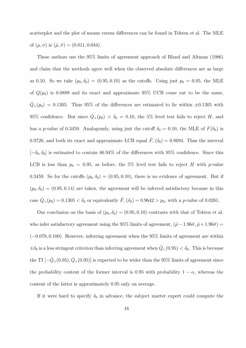
Let Θ = {(µ, σ) : |µ| < ∞, 0 < σ < ∞} be the parameter space. Also let ΘH and ΘK

be the subsets of Θ representing the regions under H and K, respectively, and ΘB be the

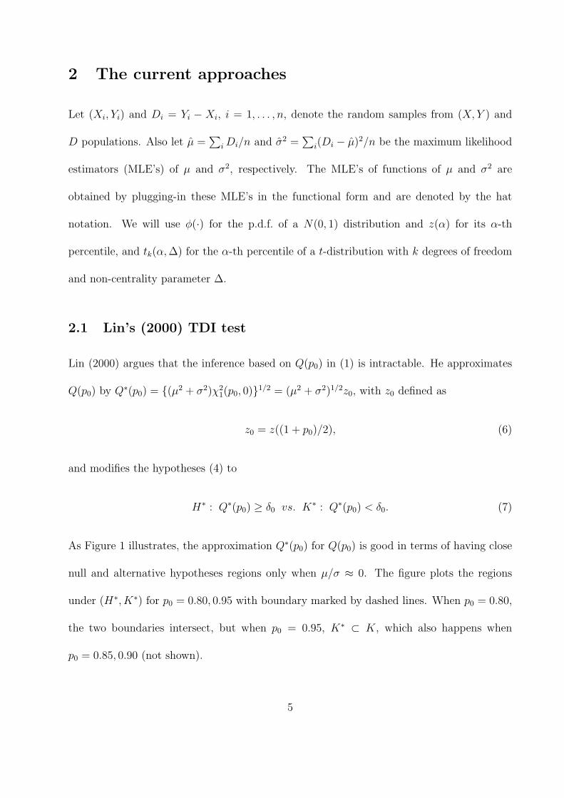
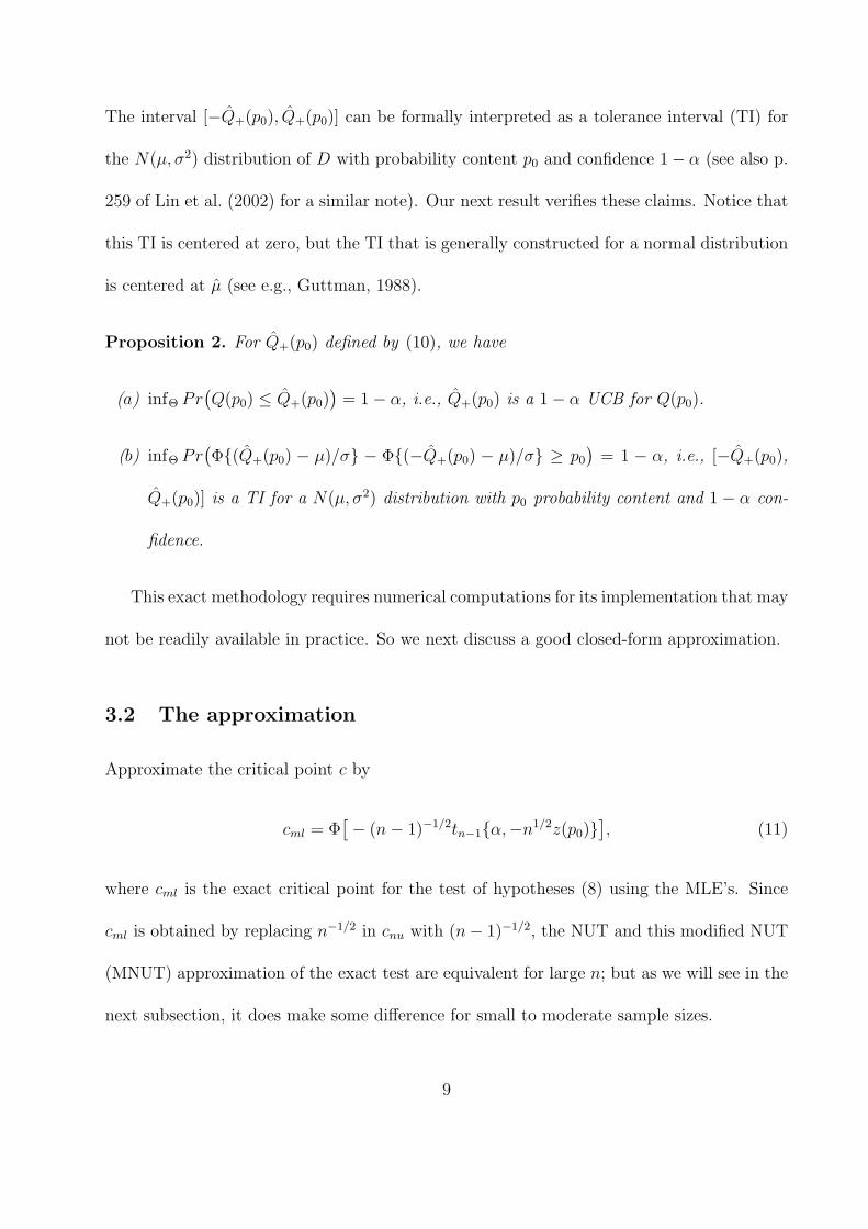
boundary of H. These regions can be visualized through the solid curves in Figure 1 for

p0 = 0.80, 0.95. Notice that they are symmetric in µ about zero.

[Figure 1 about here.]

Lin (2000) suggests a large sample test for the hypotheses (4) and we refer to it as

the TDI test. Lin et al. (2002) suggest a large sample test for (5), and we call it the

CP test. They also conclude that these tests are more powerful for inferring satisfactory

agreement than the test based on concordance correlation of Lin (1989). Sometimes the

hypotheses (5) are used to assess the individual bioequivalence of a test formulation Y of a

drug with a reference formulation X. In this context, Wang and Hwang (2001) proposed a

nearly unbiased test (NUT) and showed that it was more powerful than various other tests

3

available in the bioequivalence literature. They present numerical results to verify that a

nominal level α NUT also has size α, and call it nearly unbiased as its type-I error probability

on the boundary ΘB remains close to α.

We revisit all these tests in detail in Section 2. There we show that the TDI test for

(4) may not be consistent and may have type-I error probability of one in the limit as

n → ∞. We demonstrate that the CP test for (5) is overly conservative — its empirical

type-I error probability can be 3% or less for a nominal 5% level when n ≤ 50 and p0 ≥ 0.80.

Furthermore, even though the hypotheses (4) and (5) are equivalent, these two tests with a

common level may lead to different conclusions. We also show that the NUT can be liberal

when n is large.

In this article we discuss alternative tests that address the above concerns. Section 3

describes an exact test, which gives the same inference regarding agreement under setups (4)

and (5). To simplify its implementation, we suggest a minor modification of the NUT, say

MNUT, producing a simple closed form approximation numerically equivalent to the exact

test for n ≤ 30. We present an easy to use sample size formula for planning studies based on

this test. The MNUT can also be liberal for large n. But when both the NUT and MNUT

have their levels of significance under the nominal level, the MNUT is more nearly unbiased

and appears to be slightly, but uniformly, more powerful than the corresponding NUT. For

n ≥ 30, we provide in Section 4 an asymptotic level α parametric bootstrap-t test. It has

better properties than the asymptotic TDI and CP tests for samples of moderate sizes. In

Section 5, we illustrate the new procedures with a real data set. Section 6 contains some

concluding remarks.

4

2 The current approaches

Let (Xi, Yi) and Di = Yi − Xi, i = 1, . . . , n, denote the random samples from (X, Y ) and

D populations. Also let µ̂ =∑

i Di/n and σ̂2 =∑

i(Di − µ̂)2/n be the maximum likelihood

estimators (MLE’s) of µ and σ2, respectively. The MLE’s of functions of µ and σ2 are

obtained by plugging-in these MLE’s in the functional form and are denoted by the hat

notation. We will use φ(·) for the p.d.f. of a N(0, 1) distribution and z(α) for its α-th

percentile, and tk(α, ∆) for the α-th percentile of a t-distribution with k degrees of freedom

and non-centrality parameter ∆.

2.1 Lin’s (2000) TDI test

Lin (2000) argues that the inference based on Q(p0) in (1) is intractable. He approximates

Q(p0) by Q∗(p0) = {(µ2 + σ2)χ21(p0, 0)}1/2 = (µ2 + σ2)1/2z0, with z0 defined as

z0 = z((1 + p0)/2), (6)

and modifies the hypotheses (4) to

H∗ : Q∗(p0) ≥ δ0 vs. K∗ : Q∗(p0) < δ0. (7)

As Figure 1 illustrates, the approximation Q∗(p0) for Q(p0) is good in terms of having close

null and alternative hypotheses regions only when µ/σ ≈ 0. The figure plots the regions

under (H∗, K∗) for p0 = 0.80, 0.95 with boundary marked by dashed lines. When p0 = 0.80,

the two boundaries intersect, but when p0 = 0.95, K∗ ⊂ K, which also happens when

p0 = 0.85, 0.90 (not shown).

5

Lin’s TDI test rejects H∗ if the large-sample upper confidence bound (UCB) for Q∗(p0)

is less than δ0, i.e., exp{0.5(ln(U)+ z(1−α)V +2 ln(z0))} < δ0, where U =∑n

i=1 D2i /(n− 1)

and V 2 = 2(1 − µ̂4/U2)/(n − 1). Since this test has asymptotic level α and is consistent

for (H∗, K∗), whenever K∗ ⊂ K, there are (µ, σ) ∈ {K ∩ H∗} where the agreement is

satisfactory, but the test concludes otherwise with probability approaching one as n → ∞.

This happens with the four p0 values when µ2/σ2 >> 0. Moreover, the test may incorrectly

conclude satisfactory agreement with probability approaching one when (µ, σ) ∈ {H ∩K∗},

a possible scenario with p0 = 0.80, as Figure 1 indicates.

2.2 Lin et al.’s (2002) CP test

This test involves the estimation of F (δ0). To reduce bias, the authors estimate σ2 by

σ̂2L = nσ̂2/(n− 3). Let λ = ln{F (δ0)/(1− F (δ0))}, λ0 = ln{p0/(1− p0)} and

τ 2λ =

{(φ(du)− φ(dl)

)2+ 0.5

(duφ(du)− dlφ(dl)

)2}/{F (δ0)(1− F (δ0))

}2,

with (dl, du) defined by (2). The asymptotic level α CP test for (5) rejects H if (n−3)1/2(λ̂L−

λ0)/τ̂λ,L > z(1−α). The subscript L in the estimates implies that σ̂2L is used to estimate σ2.

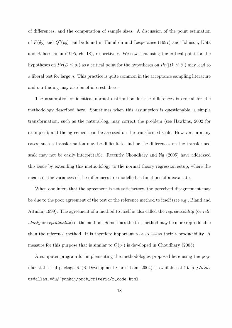
2.3 Wang and Hwang’s (2001) NUT

Here the unbiased estimator σ̃2 = nσ̂2/(n− 1) is used for σ2. Let F̃ (δ0) be the estimator of

F (δ0) that uses σ̃2 in place of σ̂2. The nominal level α NUT for (5) is: reject H if F̃ (δ0) > cnu

with cnu = Φ[− n−1/2tn−1{α,−n1/2z(p0)}

]. For this test, limσ→0 Pr(reject H |ΘB) = α.

Wang and Hwang present numerical results to argue that this test has size α. Although

this claim is true for the settings investigated by them, it is not true in general because

6

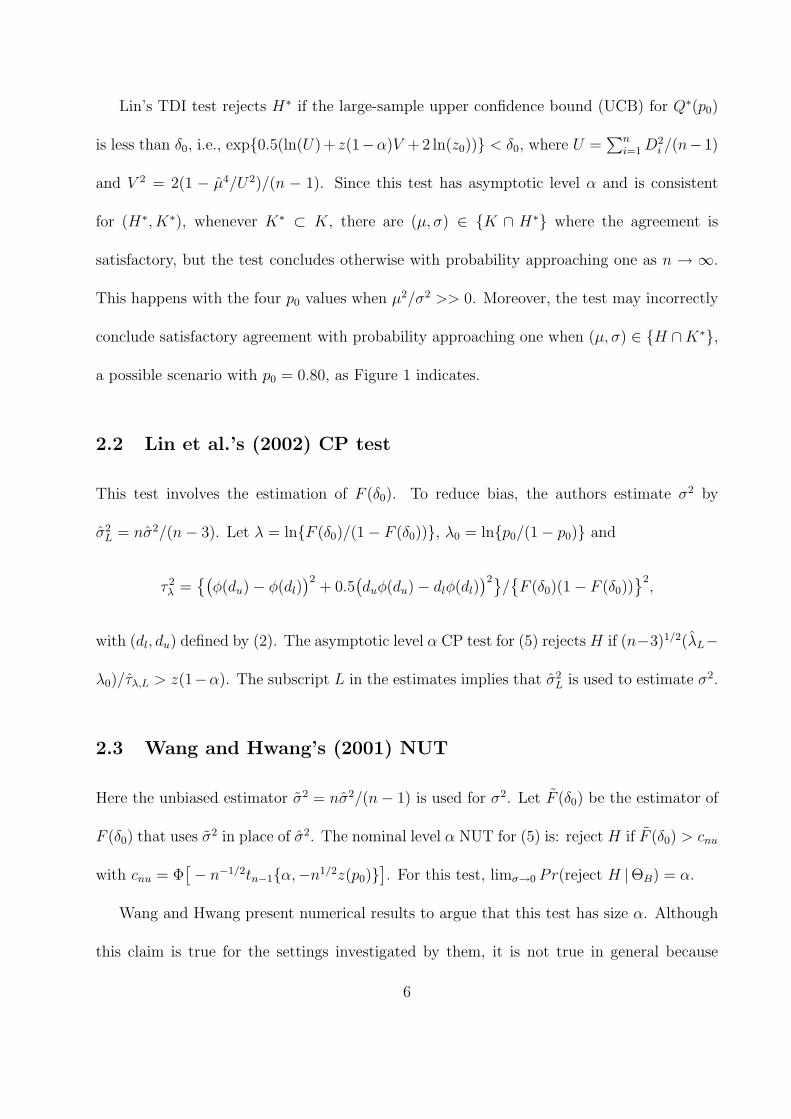
when n is large, the type-I error probability on ΘH is not maximized when σ → 0. Figure 2

plots the numerically computed minimum and maximum of these probabilities over ΘB, for

α = 5%, p0 = 0.80(0.05)0.95 and 5 ≤ n ≤ 200. The maximum exceeds the nominal 5% level

for p0 ≥ 0.85. Moreover, using standard asymptotics, it is easy to see that NUT’s asymptotic

type-I error probability on ΘB is,

1− Φ

z(1− α) φ(z(p0)

) (1 + z2(p0)/2

)1/2

((φ(du)− φ(dl)

)2+ 0.5

(duφ(du)− dlφ(dl)

)2)1/2

.

Maximizing this expression with respect to (µ, σ) ∈ ΘB gives the asymptotic size of NUT.

A numerical evaluation of these sizes for the four p0 values correspondingly produces 5.02%,

5.08%, 5.23% and 5.41%. This shows that the NUT can be liberal for large n.

[Figure 2 about here.]

It may be noted that the critical point cnu is exact for testing the hypotheses

Hnu : Pr(D ≤ δ0) ≤ p0 vs. Knu : Pr(D ≤ δ0) > p0. (8)

This technique of approximating the critical point for a test involving two-tailed probability

by the critical point for a test involving one-tailed probability is well established in the

acceptance sampling literature. There the interest lies in the parameter 1 − F (δ0), the

fraction of non-conforming items, and the test of hypotheses:

H ′ : F (δ0) ≥ p0 vs. K ′ : F (δ0) < p0,

where 1−p0 is an acceptable quality level. These hypotheses can be obtained by interchanging

H and K of (5). In acceptance sampling, it is also well-known that the tests based on

MLE’s are better than the one using the unbiased estimator of σ2 (see e.g., Hamilton and

Lesperance, 1995). This motivates some of our results in the next section.

7

3 An exact test and its approximation for n ≤ 30

3.1 The test

A size α test for (4) and (5) based on the exact distribution for the statistic F̂ (δ0) is the

following: reject H if F̂ (δ0) > c, where the critical point c is such that supΘHPr(F̂ (δ0) >

c) = α. The following result gives the power function of this test.

Proposition 1. For a fixed (µ, σ) ∈ Θ, we have

Pr(F̂ (δ0) > c) =

∫ m

0

[Φ

{n1/2

(t(σw1)−µ

)/σ

}−Φ{n1/2

(− t(σw1)−µ)/σ

}]hn−1(w)dw, (9)

where m = (nδ20)/

{σz

((1 + c)/2

)}2, w1 = (w/n)1/2, t(s) is the non-negative solution of

Φ((δ0 − t)/s

)− Φ((−δ0 − t)/s

)= c,

for t, and hn−1 is the p.d.f. of a χ2n−1-distribution. This probability function is symmetric in

µ about zero, and subject to (µ, σ) ∈ ΘH , it is maximized on ΘB.

This probability remains invariant under the transformation of D to D/δ0. After this

rescaling, H and K of (5) respectively become H1 : F1(1) ≤ p0 and K1 : F1(1) > p0, say,

where F1 is the c.d.f. of |D|/δ0. As a result, the critical points for testing (H, K) and (H1, K1)

are the same. Thus c does not depend on δ0, and in particular, one can take δ0 = 1 for its

computation by solving supΘBPr(F̂ (δ0) > c) = α. Note, however, that the value of (µ, σ)

that maximizes the probability on the LHS is not available in a closed form. So one must

use numerical maximization for this purpose.

Once c is available, the 1− α UCB for Q(p0), say Q̂+(p0), can simply be obtained as:

Q̂+(p0) = σ̂{χ21(c, µ̂

2/σ̂2)}1/2. (10)

8

The interval [−Q̂+(p0), Q̂+(p0)] can be formally interpreted as a tolerance interval (TI) for

the N(µ, σ2) distribution of D with probability content p0 and confidence 1− α (see also p.

259 of Lin et al. (2002) for a similar note). Our next result verifies these claims. Notice that

this TI is centered at zero, but the TI that is generally constructed for a normal distribution

is centered at µ̂ (see e.g., Guttman, 1988).

Proposition 2. For Q̂+(p0) defined by (10), we have

(a) infΘ Pr(Q(p0) ≤ Q̂+(p0)

)= 1− α, i.e., Q̂+(p0) is a 1− α UCB for Q(p0).

(b) infΘ Pr(Φ{(Q̂+(p0) − µ)/σ} − Φ{(−Q̂+(p0) − µ)/σ} ≥ p0

)= 1 − α, i.e., [−Q̂+(p0),

Q̂+(p0)] is a TI for a N(µ, σ2) distribution with p0 probability content and 1− α con-

fidence.

This exact methodology requires numerical computations for its implementation that may

not be readily available in practice. So we next discuss a good closed-form approximation.

3.2 The approximation

Approximate the critical point c by

cml = Φ[− (n− 1)−1/2tn−1{α,−n1/2z(p0)}

], (11)

where cml is the exact critical point for the test of hypotheses (8) using the MLE’s. Since

cml is obtained by replacing n−1/2 in cnu with (n− 1)−1/2, the NUT and this modified NUT

(MNUT) approximation of the exact test are equivalent for large n; but as we will see in the

next subsection, it does make some difference for small to moderate sample sizes.

9

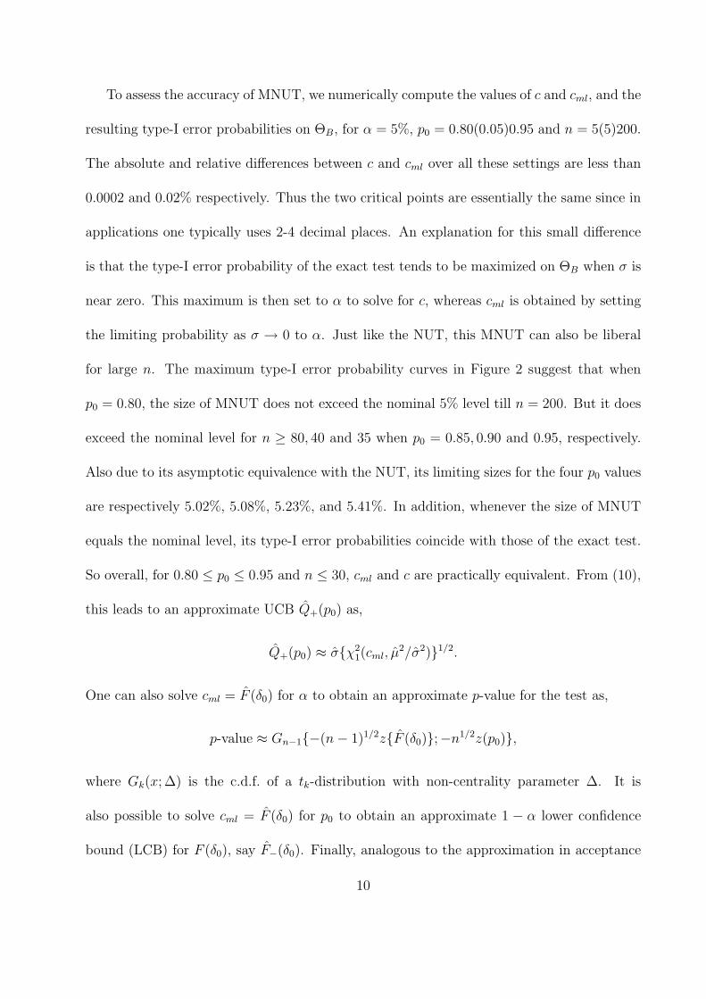
To assess the accuracy of MNUT, we numerically compute the values of c and cml, and the

resulting type-I error probabilities on ΘB, for α = 5%, p0 = 0.80(0.05)0.95 and n = 5(5)200.

The absolute and relative differences between c and cml over all these settings are less than

0.0002 and 0.02% respectively. Thus the two critical points are essentially the same since in

applications one typically uses 2-4 decimal places. An explanation for this small difference

is that the type-I error probability of the exact test tends to be maximized on ΘB when σ is

near zero. This maximum is then set to α to solve for c, whereas cml is obtained by setting

the limiting probability as σ → 0 to α. Just like the NUT, this MNUT can also be liberal

for large n. The maximum type-I error probability curves in Figure 2 suggest that when

p0 = 0.80, the size of MNUT does not exceed the nominal 5% level till n = 200. But it does

exceed the nominal level for n ≥ 80, 40 and 35 when p0 = 0.85, 0.90 and 0.95, respectively.

Also due to its asymptotic equivalence with the NUT, its limiting sizes for the four p0 values

are respectively 5.02%, 5.08%, 5.23%, and 5.41%. In addition, whenever the size of MNUT

equals the nominal level, its type-I error probabilities coincide with those of the exact test.

So overall, for 0.80 ≤ p0 ≤ 0.95 and n ≤ 30, cml and c are practically equivalent. From (10),

this leads to an approximate UCB Q̂+(p0) as,

Q̂+(p0) ≈ σ̂{χ21(cml, µ̂

2/σ̂2)}1/2.

One can also solve cml = F̂ (δ0) for α to obtain an approximate p-value for the test as,

p-value ≈ Gn−1{−(n− 1)1/2z{F̂ (δ0)};−n1/2z(p0)},

where Gk(x; ∆) is the c.d.f. of a tk-distribution with non-centrality parameter ∆. It is

also possible to solve cml = F̂ (δ0) for p0 to obtain an approximate 1 − α lower confidence

bound (LCB) for F (δ0), say F̂−(δ0). Finally, analogous to the approximation in acceptance

10

sampling (see Hamilton and Lesperance, 1995), the smallest sample size that ensures at least

1− β (> α) power for the exact level α test at F (δ0) = p1 (> p0) can be approximated as,

n ≈(

1 +k2

2

)(z(1− α) + z(1− β)

z(1− p0)− z(1− p1)

)2

; k =z(1− β)z(1− p0) + z(1− α)z(1− p1)

z(1− α) + z(1− β).

This simple approximation is also quite good as evident from Table 1 where the exact and

approximate values of n are presented for (α, 1−β) = (5%, 80%) and several (p0, p1) settings.

The approximate n’s tend to be a little smaller than the exact ones. However, their maximum

difference is 4, which only occurs when a relatively large n is needed.

[Table 1 about here.]

3.3 Comparison

For both equivalent formulations in (4) and (5) the exact test and its MNUT approximation

would lead to the same conclusion for any data set. This is an important practical advantage

over the CP and the TDI tests.

Figure 2 also demonstrates that at every (n, p0) combination where the sizes of both

MNUT and NUT equal the nominal level, the minimum type-I error rate on ΘB for the

former is always slightly higher than the latter. In this sense, the former is more nearly

unbiased than the latter. Numerical computations indicate that the exact test and its MNUT

approximation are slightly, but uniformly, more powerful than the NUT. The maximum

power of the exact test/MNUT and the NUT seem to be the same at every F (δ0) > p0,

but the minimum power of the former is at least as large as the minimum of the latter.

The increase in the minimum power of the former is small, only under 2% for n ≤ 30.

Nevertheless, there is an important theoretical advantage. This is because the power band,

11

the graph of the gap between the minimum and the maximum of the power function against

F (δ0) (> p0), for the exact test/MNUT is thinner than the band for the NUT. When the

two maxima agree, a thinner band is desirable since it tends to treat all (µ, σ) configurations

for a given F (δ0) in a more similar way, and also tends to ensure a higher power for a larger

F (δ0) value. So overall, for n ≤ 30 and 0.80 ≤ p0 ≤ 0.95, MNUT is the best option from

both theoretical and practical considerations.

4 The bootstrap-t test for n ≥ 30

4.1 The test

Let zB(α) be the α-th percentile of the parametric bootstrap distribution of the studentized

variable n1/2{

ln(Q̂(p0)

)− ln(Q(p0)

)}/(τ̂Q/Q̂(p0)

), where

τ 2Q = σ2

((φ(qu)− φ(ql)

)2+ 0.5

(quφ(qu)− qlφ(ql)

)2)

/(φ(ql) + φ(qu)

)2; (12)

with ql = (−Q(p0)− µ)/σ and qu = (Q(p0)− µ)/σ. The approximate (1− α) level UCB for

Q(p0) obtained using the bootstrap-t method (see e.g., Efron and Tibshirani, 1993) is:

Q̂B+(p0) = exp

[{ln

(Q̂(p0)

)− zB(α)τ̂Q/(n1/2 Q̂(p0)

)}],

and the asymptotic level α bootstrap test rejects H if Q̂B+(p0) < δ0. This procedure is based

on the following result.

Proposition 3. For a fixed p0 ∈ (0, 1) and (µ, σ) ∈ Θ, the asymptotic distribution of

n1/2{

ln(Q̂(p0)

)− ln(Q(p0)

)}/(τ̂Q/Q̂(p0)

)is N(0, 1).

12

The above test is implemented on the natural-log scale as this transformation reduces

the skewness and was originally observed by Lin (2000). The approximate (1−α) level LCB

F̂B− (δ0) for F (δ0) can be graphically obtained by plotting Q̂B

+(p0) against p0 and finding the

smallest p0 for which Q̂B+(p0) ≥ δ0.

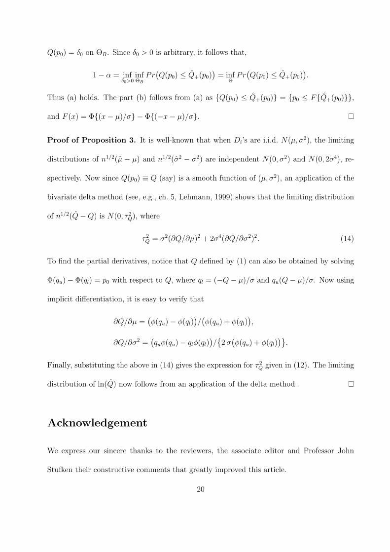
4.2 Comparison with asymptotic tests

To compare this bootstrap test with the TDI and CP tests for samples of moderate size, we

compute the empirical type-I error probabilities of the three using Monte Carlo simulation.

We restrict only to the non-positive values of µ as the distributions underlying these tests are

symmetric in µ about zero. For δ0, p0 and α, as before, we take δ0 = 1.0, p0 = 0.80(0.05)0.95

and α = 5%. Moreover, as the probabilities depend on (µ, σ) configurations that produce

the given F (δ0) = p0, the simulation is performed at 11 settings of (µ, σ) ∈ ΘB. They are

obtained by taking 11 equally spaced values of Pr(D ≥ δ0) = pu(δ0) (say) in the interval

[10−4, (1− p0)/2] and using the fact that ΘB can be characterized as the set

{0 < pu(δ0) < 1− p0, du = z

(1− pu(δ0)

), σ = 2δ0/

{du − z

(Φ(du)− p0

)}, µ = δ0 − duσ

}.

(13)

At each (µ, σ) setting, we generate a random sample of size n from a N(µ, σ2) distribution and

perform the three tests in the same way as one would do in practice with a real data set. This

process is repeated 25,000 times and the proportion of times H is rejected gives the empirical

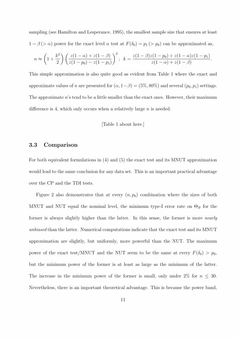
type-I error rates. They are plotted in Figure 3 for n = 30. For the computation of zB(0.05),

1999 parametric bootstrap resamples of each Monte Carlo sample is used. The numerically

computed error rates for the exact test are also included in the figure for comparison.

13

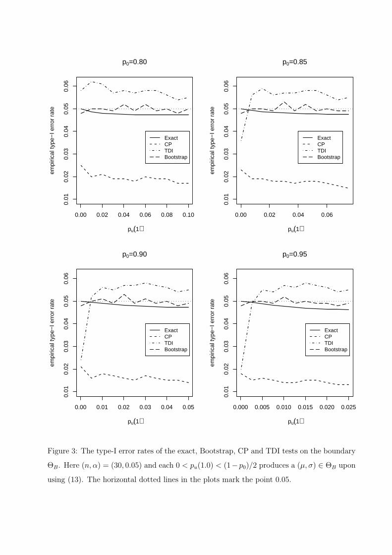
[Figure 3 about here.]

In all the four cases, the error rates for the bootstrap test remain stable around 5% and

vary between 4.8-5.3%. For the CP test, they generally lie between 1%-2%. For the TDI

test, as expected from the discussion in Section 2.1, their variation depends on the following

scenarios: (i) pu(1.0) ≈ 0 (i.e., µ2/σ2 >> 0) and p0 = 0.80; (ii) pu(1.0) ≈ 0 and p0 ≥ 0.85;

(iii) pu(1.0) ≈ (1 − p0)/2 (i.e., µ2/σ2 ≈ 0). The rates mostly lie between 5.7-6.2% for (i),

2.5-5.6% for (ii), and 5.4-5.7% for (iii). Thus, on the whole, the TDI test appears liberal.

The above pattern does not change much for the bootstrap and CP tests for n = 50, 100

(results not shown) except that the error rates come closer to the nominal 5%. However, for

these sample sizes, the rates for the TDI test, increase towards one for (i), decrease towards

zero for (ii), and come closer to 5% for (iii). This clearly demonstrates that the bootstrap

test is remarkably accurate and is the best among the three for moderate sample sizes. For

n under 30, it tends to be liberal and is not recommended. Additionally, a simulation based

power comparison for 30 ≤ n ≤ 100 indicates that it is more powerful than the CP test. This

is anticipated since the latter is overly conservative. Such a comparison of the bootstrap test

with the TDI test is not realistic due to the liberal nature of the latter.

Remark 1. This bootstrap test outperforms several other large-sample tests in moderate

sample performance. The list includes the test with z(α) in place of zB(α), the tests based

on the minimum variance unbiased estimator and the MLE of F (δ0), among others. Some

of these results are available in Choudhary and Nagaraja (2003).

Remark 2. We also computed the empirical type-I error rates at the settings studied by

Lin et al. (2002) in their Tables 2 and 3. These rates are also found to be less than 3%

14

for a nominal 5% level. They do not agree well with those reported in Lin et al. because

for computing empirical rates they use the true value of τλ whereas the CP test statistic

(n− 3)1/2(λ̂L − λ0)/τ̂λ,L that we use has its estimate in the denominator. Further, the rates

presented here for the TDI test are not comparable to those reported in Lin (2000) as we

are interested in testing hypotheses (4)-(5), but Lin focuses on (7).

4.3 Comparison with the exact test

From the Figure 3, it may be safe (up to the Monte Carlo error) to conclude that the type-I

error rates of the bootstrap test remain closer to the nominal level than those for the exact

test. It also appears that the former is slightly more powerful than the latter when n is

moderately large. The increase in power is up to about 1.5% for n = 30. Further since the

bootstrap test can be easily implemented, it provides a better option than the exact test for

n ≥ 30. One disadvantage, however, of the former is that a straightforward approach for

estimating sample size is not available — it would involve a great deal of computation.

5 An Application

Tekten et al. (2003) compare a new approach for measuring myocardial performance index

(MPI) that uses pulsed-wave tissue Doppler echocardiography with the conventional method

based on pulse Doppler. Using their data, we focus on the assessment of agreement between

the new method (Y ) and the conventional method (X) with respect to average MPI mea-

surements in the patients suffering from dilated cardiomyopathy (DCMP). There are n = 15

pairs of MPI measurements ranging between 0.50 to 1.20, and have correlation 0.95. Their

15

scatterplot and the plot of means versus differences can be found in Tekten et al. The MLE

of (µ, σ) is (µ̂, σ̂) = (0.011, 0.044).

These authors use the 95% limits of agreement approach of Bland and Altman (1986)

and claim that the methods agree well when the observed absolute differences are as large

as 0.10. So we take (p0, δ0) = (0.95, 0.10) as the cutoffs. Using just p0 = 0.95, the MLE

of Q(p0) is 0.0889 and its exact and approximate 95% UCB come out to be the same,

Q̂+(p0) = 0.1305. Thus 95% of the differences are estimated to lie within ±0.1305 with

95% confidence. But since Q̂+(p0) > δ0 = 0.10, the 5% level test fails to reject H, and

has a p-value of 0.3459. Analogously, using just the cutoff δ0 = 0.10, the MLE of F (δ0) is

0.9726, and both its exact and approximate LCB equal F̂−(δ0) = 0.8694. Thus the interval

[−δ0, δ0] is estimated to contain 86.94% of the differences with 95% confidence. Since this

LCB is less than p0 = 0.95, as before, the 5% level test fails to reject H with p-value

0.3459. So for the cutoffs (p0, δ0) = (0.95, 0.10), there is no evidence of agreement. But if

(p0, δ0) = (0.95, 0.14) are taken, the agreement will be inferred satisfactory because in this

case Q̂+(p0) = 0.1305 < δ0 or equivalently F̂−(δ0) = 0.9642 > p0, with a p-value of 0.0261.

Our conclusion on the basis of (p0, δ0) = (0.95, 0.10) contrasts with that of Tekten et al.

who infer satisfactory agreement using the 95% limits of agreement, (µ̂−1.96σ̃, µ̂+1.96σ̃) =

(−0.078, 0.100). However, inferring agreement when the 95% limits of agreement are within

±δ0 is a less stringent criterion than inferring agreement when Q̂+(0.95) < δ0. This is because

the TI [−Q̂+(0.95), Q̂+(0.95)] is expected to be wider than the 95% limits of agreement since

the probability content of the former interval is 0.95 with probability 1 − α, whereas the

content of the latter is approximately 0.95 only on average.

If it were hard to specify δ0 in advance, the subject matter expert could compute the

16

TI [−Q̂+(p0), Q̂+(p0)] for a given p0; and judge whether a difference in this interval is small

enough to be clinically unimportant. An affirmative answer means that the agreement is

inferred satisfactory. This way the assessment of agreement can be accomplished without

explicitly specifying a δ0, provided a p0 can be specified.

Table 2 compares the bounds Q̂+(0.95), F̂−(0.10) and F̂−(0.14) derived using various

methods discussed in this article. The UCB and LCB from the NUT are respectively slightly

larger and smaller than those for the exact test or its MNUT approximation. This is expected

as the latter are slightly more powerful than the former. Further since n = 15 is not large, we

do not expect the asymptotic approaches to work well, but the bootstrap and TDI bounds

are not far from the exact ones. The latter performs well because µ̂2/σ̂2 = 0.062 ≈ 0. The

CP bounds are quite off. The directions of the differences between these bounds and the

exact ones are consistent with our earlier observation on their moderate sample performance.

[Table 2 about here.]

6 Concluding remarks

In this article, we considered the problem of assessing agreement between two methods of

continuous measurement. Assuming that the differences of the paired measurements are

i.i.d. normal, we concentrated on the probability criteria approach that infers satisfactory

agreement between the methods when a sufficiently large proportion of differences lie within

an acceptable margin. We evaluated several tests of hypotheses (H,K) in this context and

proposed alternatives. We also discussed the construction of the relevant confidence bounds

for the quantile function Q(p0) and the c.d.f. F (δ0), the tolerance interval for the distribution

17

of differences, and the computation of sample sizes. A discussion of the point estimation

of F (δ0) and Q2(p0) can be found in Hamilton and Lesperance (1997) and Johnson, Kotz

and Balakrishnan (1995, ch. 18), respectively. We saw that using the critical point for the

hypotheses on Pr(D ≤ δ0) as a critical point for the hypotheses on Pr(|D| ≤ δ0) may lead to

a liberal test for large n. This practice is quite common in the acceptance sampling literature

and our finding may also be of interest there.

The assumption of identical normal distribution for the differences is crucial for the

methodology described here. Sometimes when this assumption is questionable, a simple

transformation, such as the natural-log, may correct the problem (see Hawkins, 2002 for

examples); and the agreement can be assessed on the transformed scale. However, in many

cases, such a transformation may be difficult to find or the differences on the transformed

scale may not be easily interpretable. Recently Choudhary and Ng (2005) have addressed

this issue by extending this methodology to the normal theory regression setup, where the

means or the variances of the differences are modelled as functions of a covariate.

When one infers that the agreement is not satisfactory, the perceived disagreement may

be due to the poor agreement of the test or the reference method to itself (see e.g., Bland and

Altman, 1999). The agreement of a method to itself is also called the reproducibility (or reli-

ability or repeatability) of the method. Sometimes the test method may be more reproducible

than the reference method. It is therefore important to also assess their reproducibility. A

measure for this purpose that is similar to Q(p0) is developed in Choudhary (2005).

A computer program for implementing the methodologies proposed here using the pop-

ular statistical package R (R Development Core Team, 2004) is available at http://www.

utdallas.edu/~pankaj/prob_criteria/r_code.html.

18

Appendix

Proof of Proposition 1. First observe that F (δ0) = Φ((δ0 − µ)/σ

) − Φ((−δ0 − µ)/σ

)

is a decreasing function of σ for a fixed µ, and is also decreasing function of |µ| for a

fixed σ. Thus taking µ = 0 maximizes F (δ0) over µ. Setting this maximum F (δ0) equal

to p0 and solving for σ we get σ = δ0/z0, where z0 is defined in (6). Now for a fixed

σ < δ0/z0, let a(σ) be the non-negative solution of F (δ0) = p0 with respect to µ. As a result

ΘK ={(µ, σ) : σ < δ0/z0, |µ| < a(σ)

}represents the region where F (δ0) > p0.

This argument also shows that the event {F̂ (δ0) > c} = {σ̂ < δ0/z((1+c)/2

), |µ̂| < t(σ̂)}.

The probability expression now follows since W = nσ̂2/σ2 ∼ χ2n−1, Z = n1/2(µ̂ − µ)/σ ∼

N(0, 1), and they are independent. The symmetry can be checked by replacing µ with −µ

and using the fact that Φ(x) = 1− Φ(−x).

For the next part, we write the null region as ΘH = {(µ, σ) : σ < δ0/z0, |µ| ≥ a(σ)} ∪

{(µ, σ) : σ ≥ δ0/z0} = ω1 ∪ ω2 (say). Further in (9): (i) the upper limit of integration is a

decreasing function for σ, (ii) when σ remains fixed, the integrand is a decreasing function

for |µ|, and (iii) when µ = 0, the integrand is a decreasing function of σ. So clearly in ω1, the

probability is maximized when |µ| = a(σ), and in ω2 it is maximized when µ = 0, σ = δ0/z0.

Thus in both cases the maximum occurs on the boundary.

Proof of Proposition 2. (a) Recall that c is the critical point of the size α test of (5) for

a fixed (p0 > 0.5, δ0 > 0), and the size is attained on the boundary ΘB of H. Hence we have,

1− α = infΘB

Pr(F̂ (δ0) ≤ c

)= inf

ΘB

Pr(δ0 ≤ F̂−1(c)Q̂+(p0)

)= inf

ΘB

Pr(Q(p0) ≤ Q̂+(p0)

),

where F̂ (·) is the c.d.f. of |D| when (µ, σ) = (µ̂, σ̂), and the last equality holds because

19

Q(p0) = δ0 on ΘB. Since δ0 > 0 is arbitrary, it follows that,

1− α = infδ0>0

infΘB

Pr(Q(p0) ≤ Q̂+(p0)

)= inf

ΘPr

(Q(p0) ≤ Q̂+(p0)

).

Thus (a) holds. The part (b) follows from (a) as {Q(p0) ≤ Q̂+(p0)} = {p0 ≤ F{Q̂+(p0)}},

and F (x) = Φ{(x− µ)/σ} − Φ{(−x− µ)/σ}.

Proof of Proposition 3. It is well-known that when Di’s are i.i.d. N(µ, σ2), the limiting

distributions of n1/2(µ̂ − µ) and n1/2(σ̂2 − σ2) are independent N(0, σ2) and N(0, 2σ4), re-

spectively. Now since Q(p0) ≡ Q (say) is a smooth function of (µ, σ2), an application of the

bivariate delta method (see, e.g., ch. 5, Lehmann, 1999) shows that the limiting distribution

of n1/2(Q̂−Q) is N(0, τ 2Q), where

τ 2Q = σ2(∂Q/∂µ)2 + 2σ4(∂Q/∂σ2)2. (14)

To find the partial derivatives, notice that Q defined by (1) can also be obtained by solving

Φ(qu)− Φ(ql) = p0 with respect to Q, where ql = (−Q− µ)/σ and qu(Q− µ)/σ. Now using

implicit differentiation, it is easy to verify that

∂Q/∂µ =(φ(qu)− φ(ql)

)/(φ(qu) + φ(ql)

),

∂Q/∂σ2 =(quφ(qu)− qlφ(ql)

)/{2 σ

(φ(qu) + φ(ql)

)}.

Finally, substituting the above in (14) gives the expression for τ 2Q given in (12). The limiting

distribution of ln(Q̂) now follows from an application of the delta method.

Acknowledgement

We express our sincere thanks to the reviewers, the associate editor and Professor John

Stufken their constructive comments that greatly improved this article.

20

References

Bland, J. M. and Altman, D. G. (1986). Statistical methods for assessing agreement between

two methods of clinical measurement. Lancet i, 307–310.

Choudhary, P. K. (2005). A tolerance interval approach for assessment of agreement in

method comparison studies with repeated measurements. Submitted.

Choudhary, P. K. and Nagaraja, H. N. (2003). Assessing agreement using coverage proba-

bility. Technical Report 721. Ohio State University, Columbus, OH.

Choudhary, P. K. and Ng, H. K. T. (2005). Assessment of agreement under non-standard con-

ditions using regression models for mean and variance. Biometrics doi: 10.1111/j.1541-

0420.2005.00422.x.

Efron, B. and Tibshirani, R. J. (1993). An Introduction to the Bootstrap. Chapman &

Hall/CRC, New York.

Guttman, I. (1988). Statistical tolerance regions. In Encyclopedia of Statistical Sciences,

Vol. 9, pp. 272-287, Kotz, S., Johnson, N. L. and Read, C. B. (Editors), John Wiley,

New York.

Hamilton, D. C. and Lesperance, M. L. (1995). A comparison of methods for univariate and

multivariate acceptance sampling by variables. Technometrics 37, 329–339.

Hamilton, D. C. and Lesperance, M. L. (1997). A comparison of estimators of the proportion

nonconforming in univariate and multivariate normal samples. Journal of Statistical

Computations and Simulations 59, 333–348.

21

Hawkins, D. M. (2002). Diagnostics for conformity of paired quantitative measurements.

Statistics in Medicine 21, 1913–1935.

Johnson, N. L., Kotz, S. and Balakrishnan, N. (1995). Continuous Univariate Distributions,

Vol. 2, 2nd edn. John Wiley, New York.

Lin, L. I. (1989). A concordance correlation coefficient to evaluate reproducibility. Biometrics

45, 255–268. Corrections: 2000, 56:324-325.

Lin, L. I. (2000). Total deviation index for measuring individual agreement with applications

in laboratory performance and bioequivalence. Statistics in Medicine 19, 255–270.

Lin, L. I., Hedayat, A. S., Sinha, B. and Yang, M. (2002). Statistical methods in assess-

ing agreement: Models, issues and tools. Journal of American Statistical Association

97, 257–270.

R Development Core Team (2004). R: A language and environment for statistical computing.

R Foundation for Statistical Computing. Vienna, Austria. http://www.R-project.org.

Tekten, T., Onbasili, A. O., Ceyhan, C., Unal, S. and Discigil, B. (2003). Novel approach to

measure myocardial performance index: Pulsed-wave tissue Doppler echocardiopraphy.

Echocardiography 20, 503–510.

Wang, W. and Hwang, J. T. G. (2001). A nearly unbiased test for individual bioequivalence

problems using probability criteria. Journal of Statistical Planning and Inference 99, 41–

58.

22

−1.0 −0.5 0.0 0.5 1.0

0.0

0.2

0.4

0.6

0.8

µ

σ

(H,K)(H*,K*)

Figure 1: The regions under the hypotheses (H, K) of our interest, given by (4) or (5),

and those under (H∗, K∗) of Lin (2000), given by (7). The top two curves represent the

boundaries of the two null regions for p0 = 0.80, and the bottom two for p0 = 0.95. The

alternative regions lie under the respective curves. Here we have taken δ0 = 1.0, so that the

x and the y axes actually represent µ/δ0 and σ/δ0, respectively.

0 50 100 150 200

0.03

80.

042

0.04

60.

050

p0=0.80

n

min

and

max

type

−I e

rror

rat

es

ExactApproxNUT

0 50 100 150 200

0.03

80.

042

0.04

60.

050

p0=0.85

n

min

and

max

type

−I e

rror

rat

es

ExactApproxNUT

0 50 100 150 200

0.03

80.

042

0.04

60.

050

p0=0.90

n

min

and

max

type

−I e

rror

rat

es

ExactApproxNUT

0 50 100 150 200

0.03

80.

042

0.04

60.

050

p0=0.95

n

min

and

max

type

−I e

rror

rat

es

ExactApproxNUT

Figure 2: The min and max type-I error rates of the exact test, its MNUT approximation

and the NUT on the boundary ΘB as functions of n. Here the tests have the same nominal

level α = 5%. These rates are computed numerically. In case of p0 = 0.80, the three max

curves agree, and the min curves of the exact test and its approximation coincide.

0.00 0.02 0.04 0.06 0.08 0.10

0.01

0.02

0.03

0.04

0.05

0.06

p0=0.80

pu(1)

empi

rical

type

−I e

rror

rat

e

ExactCPTDIBootstrap

0.00 0.02 0.04 0.06

0.01

0.02

0.03

0.04

0.05

0.06

p0=0.85

pu(1)

empi

rical

type

−I e

rror

rat

e

ExactCPTDIBootstrap

0.00 0.01 0.02 0.03 0.04 0.05

0.01

0.02

0.03

0.04

0.05

0.06

p0=0.90

pu(1)

empi

rical

type

−I e

rror

rat

e

ExactCPTDIBootstrap

0.000 0.005 0.010 0.015 0.020 0.025

0.01

0.02

0.03

0.04

0.05

0.06

p0=0.95

pu(1)

empi

rical

type

−I e

rror

rat

e

ExactCPTDIBootstrap

Figure 3: The type-I error rates of the exact, Bootstrap, CP and TDI tests on the boundary

ΘB. Here (n, α) = (30, 0.05) and each 0 < pu(1.0) < (1− p0)/2 produces a (µ, σ) ∈ ΘB upon

using (13). The horizontal dotted lines in the plots mark the point 0.05.

F (δ0) = p1

p0 0.85 0.90 0.95 0.99

0.80 242 (240) 55 (53) 21 (19) 9 (8)

0.85 181 (177) 36 (34) 12 (11)

0.90 106 (102) 19 (17)

0.95 46 (43)

Table 1: Exact (approximate) values of smallest sample sizes that give at least 80% power

for the 5% level test of (H, K) at F (δ0) = p1. Without loss of generality δ0 = 1.0 is taken

for these computations.

Q̂+(0.95) F̂−(0.10) F̂−(0.14)

Exact 0.1305 0.8694 0.9642

MNUT 0.1305 0.8694 0.9642

NUT 0.1309 0.8672 0.9637

Bootstrap 0.1270 0.8769 0.9673

TDI 0.1255

CP 0.7950 0.9108

Table 2: The 95% confidence bounds for Q(0.95), F (0.10) and F (0.14) obtained by inverting

various tests of (H,K) for the MPI data.