Testing unit for compliance testing of frequency ...
76
Testing unit for compliance testing of frequency regulating performance of power-generating modules Master’s thesis in Electric Power Engineering Johan Olson Nils Åkesson Department of Electrical Engineering CHALMERS UNIVERSITY OF TECHNOLOGY Gothenburg, Sweden 2021
Transcript of Testing unit for compliance testing of frequency ...
DF
Testing unit for compliance testing offrequency regulating performance ofpower-generating modules
Master’s thesis in Electric Power Engineering
Johan OlsonNils Åkesson
Department of Electrical EngineeringCHALMERS UNIVERSITY OF TECHNOLOGYGothenburg, Sweden 2021

Master’s thesis 2021:EENX30
Testing unit for compliance testing offrequency regulating performance of
power-generating modules
JOHAN OLSONNILS ÅKESSON
DF
Department of Electrical EngineeringDivision of Electric Power Engineering
Chalmers University of TechnologyGothenburg, Sweden 2021
Testing unit for compliance testing of frequencyregulating performance of power-generating modules
© JOHAN OLSON, NILS ÅKESSON, 2021.
Supervisor: Andreas Petersson, Protrol Engineering ABExaminer: Massimo Bongiorno, Department of Electrical Engineering, Chalmers
Master’s Thesis 2021:EENX30Department of Electrical EngineeringDivision of Electric Power EngineeringChalmers University of TechnologySE-412 96 GothenburgTelephone +46 31 772 1000
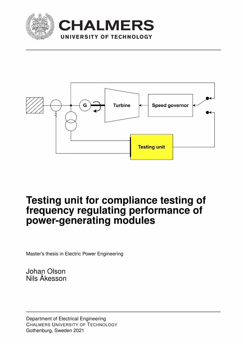
Cover: Test principle of a power-generating module and the testing unit for compli-ance testing of frequency regulating performance.
Typeset in LATEX, template by David FriskPrinted by TeknologtryckGothenburg, Sweden 2021
iv
Testing unit for compliance testing of frequencyregulating performance of power-generating modulesJOHAN OLSONNILS ÅKESSONDepartment of Electrical EngineeringChalmers University of Technology
AbstractWith more renewable energy sources and a decreasing amount of inertia in the powersystem the frequency deviations increase in amount and magnitude. New and up-dated regulations regarding frequency regulation increases the requirements of theperformance of a power-generating module’s frequency regulation. The requirementsalso increase the demand of testing the power-generating module’s compliance withthe new regulations.
The project has developed a testing unit with the purpose of testing a power gener-ation module’s performance due to frequency deviations in the power system. Thetesting unit’s functions is to measure active power output of a power generationmodule as well as providing a simulated frequency signal, representing the grid fre-quency.The software of the testing unit has been simulated in an ideal case together witha simple power-generating module model consisting of a hydro turbine governor, anexciter and a generator. The simulated voltages and currents from the generatorhave later been realised using variable voltage sources, used to test the hardwareperformance of the testing unit.
The results shows a testing unit that fulfills it’s purposes but also the importance ofusing the correct parameters in the governor depending on the purpose of the power-generating unit. The method of the project differs from the real application methodbut shows how to, in a safe manner, control a simulated model of a power-generatingmodule with external equipment.
Keywords: Frequency, RfG, FCR, PLL, Governor, Power-generating module, Speeddroop, Simulink, Matlab.
v


Testing unit for compliance testing of frequencyregulating performance of power-generating modulesJOHAN OLSONNILS ÅKESSONDepartment of Electrical EngineeringChalmers University of Technology
SammanfattningMed mer förnyelsebara energikällor och en minskande tröghetsmassa i kraftsys-temet ökar frekvensavvikelserna både i antal och i amplitud. Nya och uppdateradeföreskrifter och regulationer avseende frekvensreglering ökar kraven som ställs på enkraftproduktionsmoduls prestanda av frekvensreglering. De ökar också efterfråganpå att testa hur väl kraftproduktionsmodulen följer de nya kraven.
Projektet har utvecklat en testutrustning med syftet att testa en kraftmoduls pre-standa att reglera aktiv uteffekt givet en frekvensavvikelse i kraftsystemet. Tes-tutrustningens funktioner är att mäta aktiv effekt av en kraftproduktionsmodulsamt förse den med en simulerad frekvenssignal som representerar nätfrekvensen.Testutrustningens mjukvara har simulerats under ideella förhållanden med en enkelkraftproduktionsmodul bestående av en vattenkraftregulator, spänningsregulatoroch en generator. De simulerade spänningarna och strömmarna från generatornhar därefter realiserats med kontrollerbara spänningskällor för att testa testenhetenshårdvaruprestanda.
Resultaten visar att enhetens syften är uppfyllda samt vikten av att använda rättparametrar i turbinregulatorn beroende på kraftproduktionsmodulens syfte. Meto-den i projektet skiljer sig från tillämpningen vid ett riktigt test men visar på hur,på ett säkert sätt, en simulerad kraftproduktionsmodul kan kontrolleras med externutrustning.
Keywords: Frekvens, RfG, FCR, PLL, Turbineregulator, Kraftproduktionsmodul,Speed droop, Simulink, Matlab.
vii

AcknowledgementsWe would like to thank Andreas Petersson and Torbjörn Karlsson who have been ourguides along the way with implementing code and helping us understand it’s pur-pose. Thank you, Professor Massimo Bongiorno and Associate Professor PeiyuanChen for your interest and help with equipment used for tests at Chalmers. Allemployees at Protrol have our shared gratitude for their support and offering us agreat work environment.
"Att mäta är att veta" - Evert Agneholm
Johan Olson and Nils Åkesson, Gothenburg, February 2021
ix

Contents
List of Acronyms xiii
List of Figures xv
List of Tables xvii
1 Introduction 11.1 Background . . . . . . . . . . . . . . . . . . . . . . . . . . . . . . . . 2
1.1.1 Requirements for Generators (RfG) . . . . . . . . . . . . . . . 21.1.2 Nordic frequency market . . . . . . . . . . . . . . . . . . . . . 31.1.3 Electrical preparedness - island operation . . . . . . . . . . . . 51.1.4 Testing unit platform . . . . . . . . . . . . . . . . . . . . . . . 5
1.2 Aim . . . . . . . . . . . . . . . . . . . . . . . . . . . . . . . . . . . . 51.3 Problem definition . . . . . . . . . . . . . . . . . . . . . . . . . . . . 61.4 Limitations . . . . . . . . . . . . . . . . . . . . . . . . . . . . . . . . 61.5 Sustainability aspects . . . . . . . . . . . . . . . . . . . . . . . . . . . 7
1.5.1 Social aspects . . . . . . . . . . . . . . . . . . . . . . . . . . . 71.5.2 Ecological aspects . . . . . . . . . . . . . . . . . . . . . . . . . 81.5.3 Economic aspects . . . . . . . . . . . . . . . . . . . . . . . . . 8
2 Frequency control 92.1 Inertial response of synchronous machines at frequency deviations . . 102.2 RfG limitations . . . . . . . . . . . . . . . . . . . . . . . . . . . . . . 112.3 Frequency Containment Reserve . . . . . . . . . . . . . . . . . . . . . 122.4 Technical requirements for testing of FCR provision in the Nordic
synchronous area . . . . . . . . . . . . . . . . . . . . . . . . . . . . . 122.5 Governor and speed droop control . . . . . . . . . . . . . . . . . . . . 13
3 Test principle 153.1 Open loop operation . . . . . . . . . . . . . . . . . . . . . . . . . . . 163.2 Closed loop operation using hardware-in-the-loop . . . . . . . . . . . 17
4 Protrol’s testing unit 194.1 Hardware . . . . . . . . . . . . . . . . . . . . . . . . . . . . . . . . . 19
4.1.1 Sample rate of output file . . . . . . . . . . . . . . . . . . . . 204.2 Web interface . . . . . . . . . . . . . . . . . . . . . . . . . . . . . . . 214.3 Software development tool . . . . . . . . . . . . . . . . . . . . . . . . 21
xi
Contents
4.4 Signal processing and software implementation . . . . . . . . . . . . . 214.4.1 Synchronous coordinates . . . . . . . . . . . . . . . . . . . . . 214.4.2 Phase locked loop . . . . . . . . . . . . . . . . . . . . . . . . . 234.4.3 Instantaneous active and reactive power . . . . . . . . . . . . 254.4.4 Island operation and closed loop simulation . . . . . . . . . . 264.4.5 Discrete time low pass filter . . . . . . . . . . . . . . . . . . . 27
5 Performance testing 295.1 Measuring precision . . . . . . . . . . . . . . . . . . . . . . . . . . . . 29
5.1.1 ONLLY-AT633 and OMICRON CMC 356 . . . . . . . . . . . 305.2 Grid testing . . . . . . . . . . . . . . . . . . . . . . . . . . . . . . . . 315.3 Application testing . . . . . . . . . . . . . . . . . . . . . . . . . . . . 32
5.3.1 Simulation model in Simulink . . . . . . . . . . . . . . . . . . 335.3.2 Simulation environment and software to hardware interface . . 365.3.3 Amplifier equipment . . . . . . . . . . . . . . . . . . . . . . . 36
6 Results 376.1 Precision tests . . . . . . . . . . . . . . . . . . . . . . . . . . . . . . . 376.2 Grid tests . . . . . . . . . . . . . . . . . . . . . . . . . . . . . . . . . 406.3 Application tests . . . . . . . . . . . . . . . . . . . . . . . . . . . . . 41
6.3.1 Open loop operation . . . . . . . . . . . . . . . . . . . . . . . 426.3.2 Closed loop operation . . . . . . . . . . . . . . . . . . . . . . 48
7 Discussion 517.1 Precision of measurements . . . . . . . . . . . . . . . . . . . . . . . . 517.2 Deviation between measured and simulated values in the application
testing . . . . . . . . . . . . . . . . . . . . . . . . . . . . . . . . . . . 527.3 Simulated power-generating module or real power-generating module 527.4 Importance of parametrisation of the governor . . . . . . . . . . . . . 537.5 Future studies . . . . . . . . . . . . . . . . . . . . . . . . . . . . . . . 53
8 Conclusion 55
Bibliography 57
xii

List of Acronyms
AC Alternating currentADC Analog-to-digital converteraFRR Automatic frequency restoration reserve
CPU Central processing unit
DAC Digital-to-analog converterDC Direct current
ECU Electronic control unitEIFS Energimarknadsinspektionens författningssamling
FCR Frequency containment reserveFCR-D Frequency containment reserve-disturbanceFCR-N Frequency containment reserve-normalFFR Fast frequency reserve
HVDC High-voltage direct currentHWIL Hardware-in-the-loop
IDE Integrated development environment
MCPU Master controller processor unitmFRR Manual frequency restoration reserve
PCB Printed circuit boardPLL Phase locked loop
RfG Requirements for generators
TSO Transmission system operator
xiii

List of Acronyms
xiv
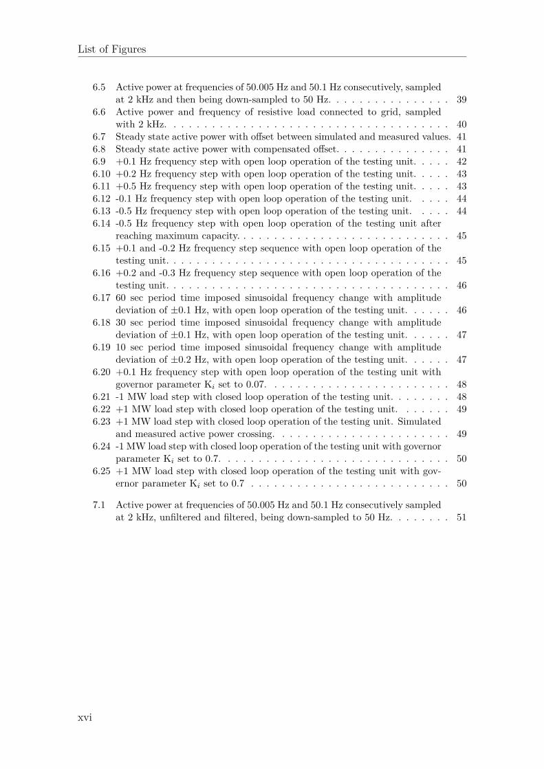
List of Figures
1.1 Frequency of the Nordic synchronous system sampled at 10 Hz for 24 hours,2019-03-04. The data was collected by Fingrid at a 400 kV substation inKangasala with local time (UTC+2) [8]. . . . . . . . . . . . . . . . . . . . . 3
1.2 Frequency of the Nordic synchronous system during 10 minutes from 12:00in Figure 1.1 [8]. . . . . . . . . . . . . . . . . . . . . . . . . . . . . . . . . . 4
1.3 Frequency of the Nordic synchronous system during 4 minutes from 14:04in Figure 1.1, with frequency drop to 49.591 Hz at 14:05:26 [8]. . . . . . . . 4
2.1 The frequency reserve activation process [12]. . . . . . . . . . . . . . . . . . 92.2 Ideal steady-state characteristics of a governor with speed droop control. . . 142.3 Simple governor model with a PI regulator including a speed droop feedback. 14
3.1 Principle description of test equipment connection. . . . . . . . . . . . . . . 163.2 A step test sequence. . . . . . . . . . . . . . . . . . . . . . . . . . . . . . . . 163.3 An imposed sinusoidal test sequence. . . . . . . . . . . . . . . . . . . . . . . 173.4 Schematic for island operation testing with HWIL. . . . . . . . . . . . . . . 173.5 A load step for island operation simulation. . . . . . . . . . . . . . . . . . . 18
4.1 Layout of the testing module. . . . . . . . . . . . . . . . . . . . . . . . . . . 204.2 Transformation from a three-phase system into αβ and dq-frame. . . . . . . 224.3 Block diagram of a phase locked loop [17]. . . . . . . . . . . . . . . . . . . . 234.4 Bode plot of the PLL described in Section 4.4.2. . . . . . . . . . . . . . . . 254.5 Measurement and tracking system including a Clarke transformation, a
Park transformation and a PLL. . . . . . . . . . . . . . . . . . . . . . . . . 25
5.1 Test setup with relay tester ONLLY-M783 and OMICRON CMC 356. Dot-ted lines are operations made in software and full lines are physical cables. . 29
5.2 Test setup with grid connection. Dotted lines are operations made in soft-ware and full lines are physical cables. . . . . . . . . . . . . . . . . . . . . . 31
5.3 Test setup with physical measurements. The simulated strong grid voltageis sent out with the DAC in MicroLabBox and the current comes from aamplified voltage from TC.ACS sent through a known resistor. Dotted linesare operations made in software and full lines are physical cables. . . . . . . 32
5.4 Simulink model of the power-generating module and the testing module. . . 34
6.1 Phase voltage Ub at 50.1 Hz, with 2 kHz sampling frequency. . . . . . . . . 376.2 Active power and frequency sampled at 2 kHz. . . . . . . . . . . . . . . . . 386.3 Step of active power and frequency with an output sample rate of 2 kHz. . 386.4 Step of active power and frequency with an output sample rate of 50 Hz. . 39
xv
List of Figures
6.5 Active power at frequencies of 50.005 Hz and 50.1 Hz consecutively, sampledat 2 kHz and then being down-sampled to 50 Hz. . . . . . . . . . . . . . . . 39
6.6 Active power and frequency of resistive load connected to grid, sampledwith 2 kHz. . . . . . . . . . . . . . . . . . . . . . . . . . . . . . . . . . . . . 40
6.7 Steady state active power with offset between simulated and measured values. 416.8 Steady state active power with compensated offset. . . . . . . . . . . . . . . 416.9 +0.1 Hz frequency step with open loop operation of the testing unit. . . . . 426.10 +0.2 Hz frequency step with open loop operation of the testing unit. . . . . 436.11 +0.5 Hz frequency step with open loop operation of the testing unit. . . . . 436.12 -0.1 Hz frequency step with open loop operation of the testing unit. . . . . 446.13 -0.5 Hz frequency step with open loop operation of the testing unit. . . . . 446.14 -0.5 Hz frequency step with open loop operation of the testing unit after
reaching maximum capacity. . . . . . . . . . . . . . . . . . . . . . . . . . . . 456.15 +0.1 and -0.2 Hz frequency step sequence with open loop operation of the
testing unit. . . . . . . . . . . . . . . . . . . . . . . . . . . . . . . . . . . . . 456.16 +0.2 and -0.3 Hz frequency step sequence with open loop operation of the
testing unit. . . . . . . . . . . . . . . . . . . . . . . . . . . . . . . . . . . . . 466.17 60 sec period time imposed sinusoidal frequency change with amplitude
deviation of ±0.1 Hz, with open loop operation of the testing unit. . . . . . 466.18 30 sec period time imposed sinusoidal frequency change with amplitude
deviation of ±0.1 Hz, with open loop operation of the testing unit. . . . . . 476.19 10 sec period time imposed sinusoidal frequency change with amplitude
deviation of ±0.2 Hz, with open loop operation of the testing unit. . . . . . 476.20 +0.1 Hz frequency step with open loop operation of the testing unit with
governor parameter Ki set to 0.07. . . . . . . . . . . . . . . . . . . . . . . . 486.21 -1 MW load step with closed loop operation of the testing unit. . . . . . . . 486.22 +1 MW load step with closed loop operation of the testing unit. . . . . . . 496.23 +1 MW load step with closed loop operation of the testing unit. Simulated
and measured active power crossing. . . . . . . . . . . . . . . . . . . . . . . 496.24 -1 MW load step with closed loop operation of the testing unit with governor
parameter Ki set to 0.7. . . . . . . . . . . . . . . . . . . . . . . . . . . . . . 506.25 +1 MW load step with closed loop operation of the testing unit with gov-
ernor parameter Ki set to 0.7 . . . . . . . . . . . . . . . . . . . . . . . . . . 50
7.1 Active power at frequencies of 50.005 Hz and 50.1 Hz consecutively sampledat 2 kHz, unfiltered and filtered, being down-sampled to 50 Hz. . . . . . . . 51
xvi
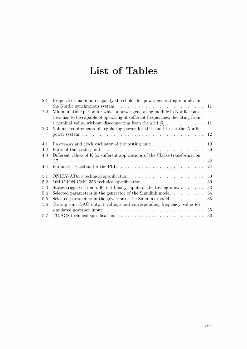
List of Tables
2.1 Proposal of maximum capacity thresholds for power-generating modules inthe Nordic synchronous system. . . . . . . . . . . . . . . . . . . . . . . . . . 11
2.2 Minimum time period for which a power-generating module in Nordic coun-tries has to be capable of operating at different frequencies, deviating froma nominal value, without disconnecting from the grid [5]. . . . . . . . . . . . 11
2.3 Volume requirements of regulating power for the countries in the Nordicpower system. . . . . . . . . . . . . . . . . . . . . . . . . . . . . . . . . . . . 12
4.1 Processors and clock oscillator of the testing unit. . . . . . . . . . . . . . . . 194.2 Ports of the testing unit. . . . . . . . . . . . . . . . . . . . . . . . . . . . . . 204.3 Different values of K for different applications of the Clarke transformation
[17]. . . . . . . . . . . . . . . . . . . . . . . . . . . . . . . . . . . . . . . . . 224.4 Parameter selection for the PLL. . . . . . . . . . . . . . . . . . . . . . . . . 24
5.1 ONLLY-AT633 technical specification. . . . . . . . . . . . . . . . . . . . . . 305.2 OMICRON CMC 356 technical specification. . . . . . . . . . . . . . . . . . 305.3 States triggered from different binary inputs of the testing unit. . . . . . . . 335.4 Selected parameters in the generator of the Simulink model. . . . . . . . . . 345.5 Selected parameters in the governor of the Simulink model. . . . . . . . . . 355.6 Testing unit DAC output voltage and corresponding frequency value for
simulated governor input. . . . . . . . . . . . . . . . . . . . . . . . . . . . . 355.7 TC.ACS technical specification. . . . . . . . . . . . . . . . . . . . . . . . . . 36
xvii

List of Tables
xviii
1Introduction
Today, the climate change forces the society to change to more carbon neutral energysources even though the production of power will vary more and introduce more instabil-ity to the system compared to before. The process of replacing the conventional thermaland nuclear power plants with renewable production units brings challenges to the system.When removing the base production units and replacing them with power electronic con-trolled power-generating modules, the total system inertia decreases. Less inertia meansless energy stored in the system and during power imbalances there will be faster devia-tions in frequency compared to power systems which has a higher amount of inertia [1].
Renewable energy sources follow a certain long-term pattern such as more wind hoursduring winter and more sun hours during the summer. The short-term pattern is morerandom due to rapid weather changes which causes imbalances in the power system andneeds to be compensated for with control equipment and production units.The load characteristic of the power system is seeing a shift as new technology has beenestablished and changes the way the loads act. The introduction of variable speed drivesmake induction motors act as a constant power sources and disconnects the spinning re-serves of kinetic energy from the system [2].
The fluctuating power generation combined with less inertia causes stress on the systemwhen balancing the supply to the demand. Frequency in the power system is a mea-surement of how well the supply and demand are matched and the system is designed tooperate at 50 Hz. The tripping of large production units or high-voltage direct current(HVDC) links are often the reason for large fluctuations and might, in the worst-casescenario, cause the frequency to drop to unacceptable levels. Off-limit frequencies mightlead disconnection of power-generating modules and loads, producing a cascade effect andwidespread power outages [3].
Frequency stability is the power system’s ability to maintain a steady frequency after asevere system disturbance resulting in an imbalance between the generation and the load.To cope with the ongoing transition to a more renewable reliant power production, thecontrol equipment for frequency stability needs to be simulated and validated for differentdynamic scenarios. The market for speed droop, ramping, frequency control reserve anddisturbance power reserve will continue to grow with more renewables along with validationof the frequency control equipment [4].
1
1. Introduction
1.1 BackgroundNew regulations, made to ensure the quality of power-generating module operation andgrid stability, has been established for power producers in Europe. The need to test power-generating modules is more dire now as verifying unit function is mandatory to enforcethe regulations.
1.1.1 Requirements for Generators (RfG)In 2016, the European commission released regulations for establishing a network code onrequirements for grid connection of generators (RfG). The requirements are set to bringharmonised standards that generators must respect in order to connect to the grid [5].
RfG should:
• Establish new rules for the interconnection of power generating modules.
• Ensure the power generators ability to contribute to the functionality of the grid.
• Increase the ability to connect renewable power production.
• Harmonise the rules for European power producers.
To reach this goal, all power production units that are rebuilt and/or being newly installedmust fulfill certain criterion in order to be connected to the grid. Among these criterionare frequency control, active power output regardless of the change in frequency, droopsettings, voltage levels and other boundaries set by the transmission system operator(TSO).The RfG is developed for the European market, but the regional or domestic marketswithin Europe may enforce more requirements as long as they are in line with the RfG.In Sweden, these requirements have been further explained in EIFS 2018:2 to be adaptedto the Nordic market [6].
2
1. Introduction
1.1.2 Nordic frequency marketThe frequency in the Nordic synchronous system fluctuates around the nominal 50 Hz. Tocope with these fluctuations, power-generating modules capable of controlling the activepower output as a response to system frequency changes are used in the system. Thefrequency regulating services used in the Nordic market are called frequency containmentreserves (FCR) and are divided into FCR-normal (FCR-N) and FCR-disturbance (FCR-D).
• FCR-N is an up- and down-regulating service with low frequency deviation thresholdset to be within ±0.1 Hz from the nominal 50 Hz.
• FCR-D is an up-regulating service that is activated for larger frequency deviationsand the threshold is set to be within -0.1 Hz and -0.5 Hz.
• FCR-D down regulation is a product soon to be introduced on the market with thethreshold set to be within +0.1 Hz and +0.5 Hz.
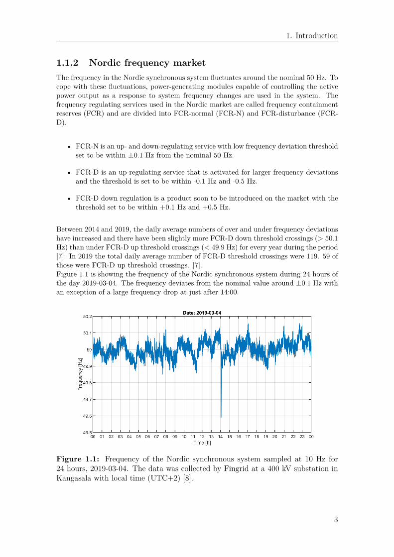
Between 2014 and 2019, the daily average numbers of over and under frequency deviationshave increased and there have been slightly more FCR-D down threshold crossings (> 50.1Hz) than under FCR-D up threshold crossings (< 49.9 Hz) for every year during the period[7]. In 2019 the total daily average number of FCR-D threshold crossings were 119. 59 ofthose were FCR-D up threshold crossings. [7].Figure 1.1 is showing the frequency of the Nordic synchronous system during 24 hours ofthe day 2019-03-04. The frequency deviates from the nominal value around ±0.1 Hz withan exception of a large frequency drop at just after 14:00.
Figure 1.1: Frequency of the Nordic synchronous system sampled at 10 Hz for24 hours, 2019-03-04. The data was collected by Fingrid at a 400 kV substation inKangasala with local time (UTC+2) [8].
3
1. Introduction
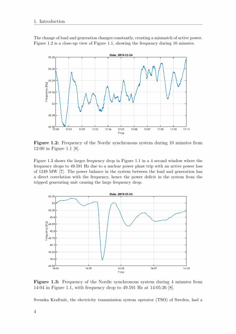
The change of load and generation changes constantly, creating a mismatch of active power.Figure 1.2 is a close-up view of Figure 1.1, showing the frequency during 10 minutes.
Figure 1.2: Frequency of the Nordic synchronous system during 10 minutes from12:00 in Figure 1.1 [8].
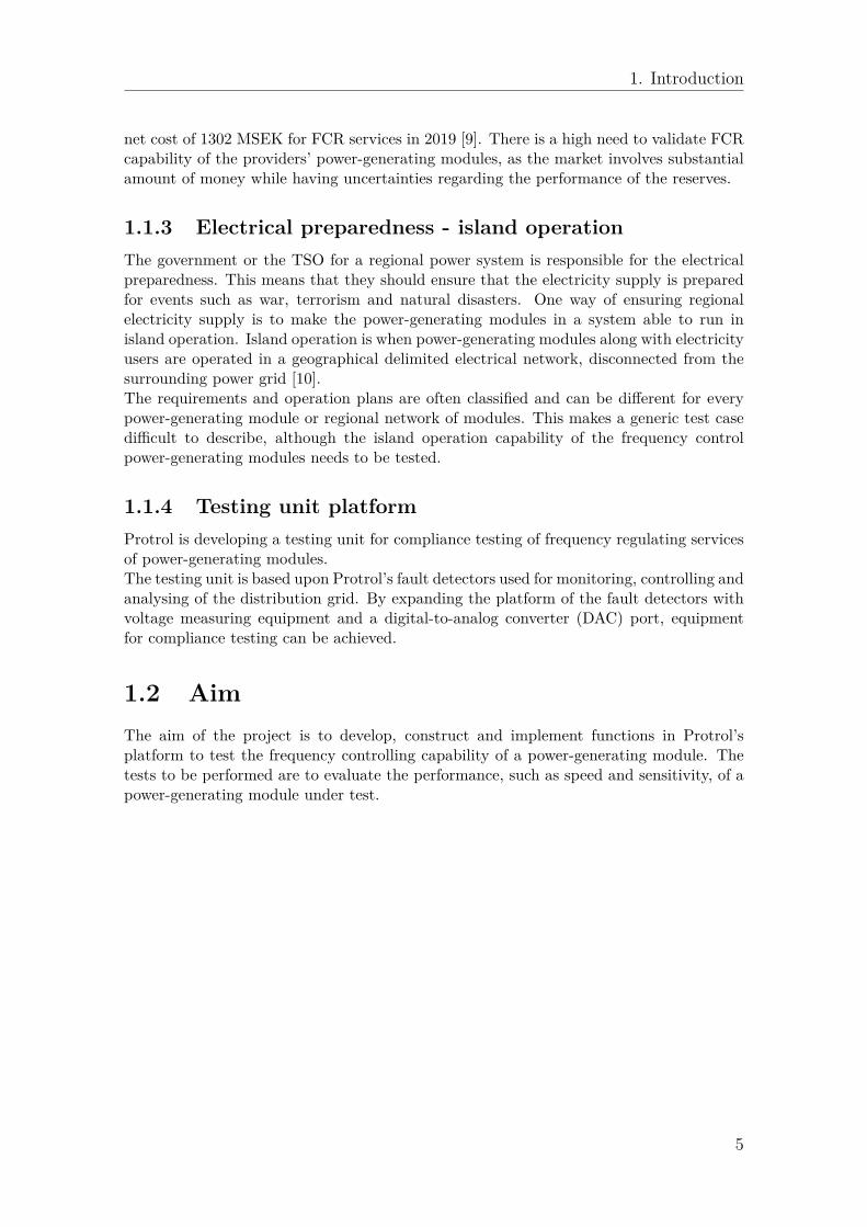
Figure 1.3 shows the larger frequency drop in Figure 1.1 in a 4 second window where thefrequency drops to 49.591 Hz due to a nuclear power plant trip with an active power lossof 1249 MW [7]. The power balance in the system between the load and generation hasa direct correlation with the frequency, hence the power deficit in the system from thetripped generating unit causing the large frequency drop.
Figure 1.3: Frequency of the Nordic synchronous system during 4 minutes from14:04 in Figure 1.1, with frequency drop to 49.591 Hz at 14:05:26 [8].
Svenska Kraftnät, the electricity transmission system operator (TSO) of Sweden, had a
4
1. Introduction
net cost of 1302 MSEK for FCR services in 2019 [9]. There is a high need to validate FCRcapability of the providers’ power-generating modules, as the market involves substantialamount of money while having uncertainties regarding the performance of the reserves.
1.1.3 Electrical preparedness - island operationThe government or the TSO for a regional power system is responsible for the electricalpreparedness. This means that they should ensure that the electricity supply is preparedfor events such as war, terrorism and natural disasters. One way of ensuring regionalelectricity supply is to make the power-generating modules in a system able to run inisland operation. Island operation is when power-generating modules along with electricityusers are operated in a geographical delimited electrical network, disconnected from thesurrounding power grid [10].The requirements and operation plans are often classified and can be different for everypower-generating module or regional network of modules. This makes a generic test casedifficult to describe, although the island operation capability of the frequency controlpower-generating modules needs to be tested.
1.1.4 Testing unit platformProtrol is developing a testing unit for compliance testing of frequency regulating servicesof power-generating modules.The testing unit is based upon Protrol’s fault detectors used for monitoring, controlling andanalysing of the distribution grid. By expanding the platform of the fault detectors withvoltage measuring equipment and a digital-to-analog converter (DAC) port, equipmentfor compliance testing can be achieved.
1.2 AimThe aim of the project is to develop, construct and implement functions in Protrol’splatform to test the frequency controlling capability of a power-generating module. Thetests to be performed are to evaluate the performance, such as speed and sensitivity, of apower-generating module under test.
5
1. Introduction
1.3 Problem definitionWith the regulations and requirements for testing of a power generating module, the mainquestion becomes:
How is the frequency regulating performance of a power generating module tested toensure the requirements of its application are met?
The focus is to develop a testing unit for validating the frequency control capabilitiesof type C and D power-generating modules, with regard to the regulations of RfG, FCRand island operation. The testing unit should be able to measure the active power out-put and send a simulated frequency signal to a power-generating module. The project isdivided into the following parts:
• Implementation of desired test methods in Protrol’s platform.
• Testing of measuring performance of the testing unit.
• Development and implementation of a simulation model of the testing unit and apower-generating module in Simulink.
• Real time simulations with a power-generating module model for application testingof the testing unit.
The chosen method of using simulations instead of measuring on a real power-generatingmodule may differ in the way the input signals to the testing unit behaves.
1.4 LimitationsThe limitations of the project are:
• The project will not include any designing of the printed circuit boards (PCBs) usedwithin the testing unit nor will it include writing the user interface of the testingmodule, as this is provided by the Protrol product development team.
• The guidelines and regulations used for the project will be ones made for the Euro-pean market and if applicable more specifically the Nordic synchronous system.
• The project will focus on implementing functions for FCR services and leave otherfrequency regulating services outside the scope.
• Power-generating modules of type A and B will not be investigated as these aresmaller units not required by RfG to provide frequency controlling services.
• Frequency dependent loads are not taken into account in closed loop operationsimulations.
6
1. Introduction
1.5 Sustainability aspectsIn order to enforce a certain level of integrity in the report and during the project, theauthors are following the IEEE Code of Ethics [11]. Here, ten guidelines are provided toensure that the work is conducted at the highest professional and ethical cautious manner,where some are more prominent for the project at hand.
"5. to seek, accept, and offer honest criticism of technical work, to acknowledge and correcterrors, to be honest and realistic in stating claims or estimates based on available data,and to credit properly the contributions of others;" [11].
Since the work is to be carried out at Protrol and is evolved around the company’s prod-ucts, it is necessary to acknowledge the material and help received from Protrol as well ascrediting other sources of information used in the project in order to ensure total trans-parency.
"3. to avoid real or perceived conflicts of interest whenever possible, and to disclose themto affected parties when they do exist;" [11].
As the master’s thesis is conducted at Protrol, the authors have responsibility towardsProtrol and Chalmers University of Technology, meaning any flaws or implication foundin the project and its end product should be disclosed and discussed between both parties.This both to give Protrol the chance of eliminating and/or avoiding any faults in theirproducts and to give the seat of learning from Chalmers the full insight concerning pitfallsregarding future works in the area.
1.5.1 Social aspectsBy ensuring that a power-generating module is up to par with the high standard of op-eration the network code has set, more renewable sources can be integrated into the gridwithout compromising the stability. Since most renewable sources fluctuate in productionas they are dependent of the environment (sun, wind and waves) they are inherently un-stable in output power and or frequency. Assuring the high operating standard is thereforekey to foresee and provide the needed generation with given environmental circumstancesand power demand from the market.
Introducing a power-generating module testing unit, which can be permanently installedand remotely operated, will pave way for more frequent testing of a module’s operatingcondition. With a grid powered only by highly functioning modules, the stability of thegrid will increase and further contribute to less power outages, giving the end users safetyand increased quality of life.
7
1. Introduction
1.5.2 Ecological aspectsRegulations such as RfG are meant to ease the integration of renewable power productionand enable more efficient use of the existing grid. By enabling the shift from old energysources to new renewable ones without losing the stability in the grid is key for a smallercarbon footprint in a society run on electricity. By ensuring that modules are functioningin accordance with the specified criterion, the need for buying power from regions withless renewable sources when demand is higher than local production is also reduced.
1.5.3 Economic aspectsThe process of testing a power-generating module today is time consuming as the testequipment is ungainly and the process of setting up the equipment, testing and disassem-ble everything once done may take days in man hours. When utilising a permanentlyinstalled module which can take measurements remotely, the total testing time is substan-tially reduced.
The regulations in the RfG states that all newly installed power-generating modules areto be tested as well as older modules which are being rebuilt or modified. By testingthe power-generating modules more frequently, occurring faults or non-optimized controlparameters may be found, which in turn can lead to less maintenance/reparation costs.
8
2Frequency control
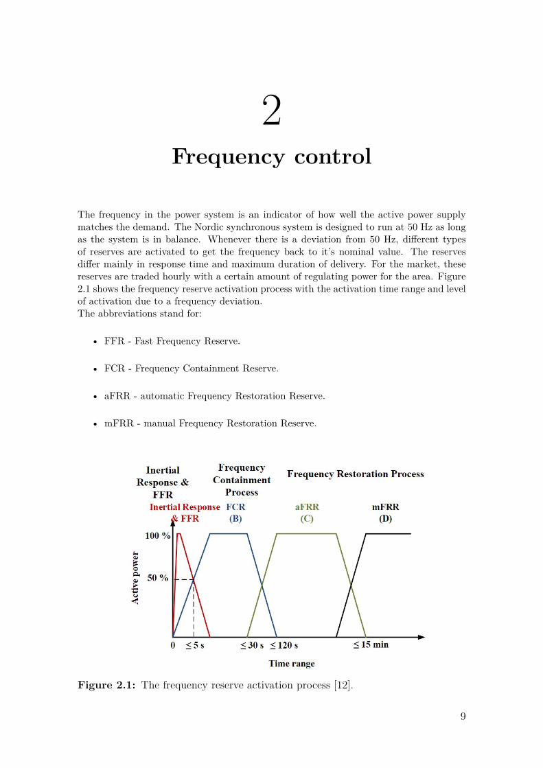
The frequency in the power system is an indicator of how well the active power supplymatches the demand. The Nordic synchronous system is designed to run at 50 Hz as longas the system is in balance. Whenever there is a deviation from 50 Hz, different typesof reserves are activated to get the frequency back to it’s nominal value. The reservesdiffer mainly in response time and maximum duration of delivery. For the market, thesereserves are traded hourly with a certain amount of regulating power for the area. Figure2.1 shows the frequency reserve activation process with the activation time range and levelof activation due to a frequency deviation.The abbreviations stand for:
• FFR - Fast Frequency Reserve.
• FCR - Frequency Containment Reserve.
• aFRR - automatic Frequency Restoration Reserve.
• mFRR - manual Frequency Restoration Reserve.
Figure 2.1: The frequency reserve activation process [12].
9
2. Frequency control
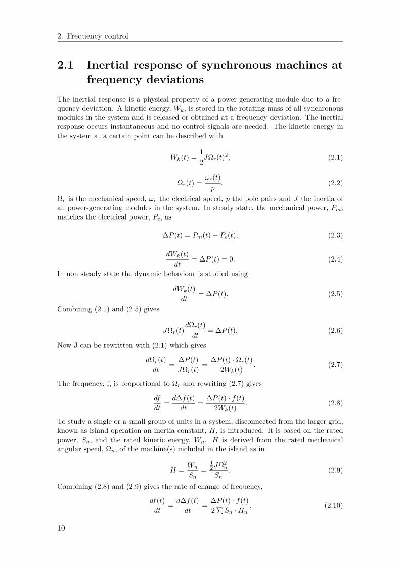
2.1 Inertial response of synchronous machines atfrequency deviations
The inertial response is a physical property of a power-generating module due to a fre-quency deviation. A kinetic energy, Wk, is stored in the rotating mass of all synchronousmodules in the system and is released or obtained at a frequency deviation. The inertialresponse occurs instantaneous and no control signals are needed. The kinetic energy inthe system at a certain point can be described with
Wk(t) =12JΩr(t)2, (2.1)
Ωr(t) =ωr(t)p
. (2.2)
Ωr is the mechanical speed, ωr the electrical speed, p the pole pairs and J the inertia ofall power-generating modules in the system. In steady state, the mechanical power, Pm,matches the electrical power, Pe, as
∆P (t) = Pm(t)− Pe(t), (2.3)
dWk(t)dt
= ∆P (t) = 0. (2.4)
In non steady state the dynamic behaviour is studied using
dWk(t)dt
= ∆P (t). (2.5)
Combining (2.1) and (2.5) gives
JΩr(t)dΩr(t)dt
= ∆P (t). (2.6)
Now J can be rewritten with (2.1) which gives
dΩr(t)dt
= ∆P (t)JΩr(t)
= ∆P (t) · Ωr(t)2Wk(t)
. (2.7)
The frequency, f, is proportional to Ωr and rewriting (2.7) gives
df
dt= d∆f(t)
dt= ∆P (t) · f(t)
2Wk(t). (2.8)
To study a single or a small group of units in a system, disconnected from the larger grid,known as island operation an inertia constant, H, is introduced. It is based on the ratedpower, Sn, and the rated kinetic energy, Wn. H is derived from the rated mechanicalangular speed, Ωn, of the machine(s) included in the island as in
H = Wn
Sn=
12JΩ2
n
Sn. (2.9)
Combining (2.8) and (2.9) gives the rate of change of frequency,
df(t)dt
= d∆f(t)dt
= ∆P (t) · f(t)2∑Sn ·Hn
. (2.10)
10
2. Frequency control
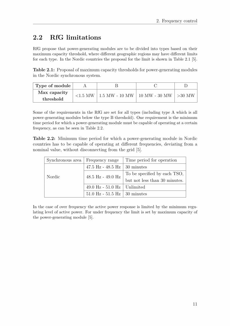
2.2 RfG limitationsRfG propose that power-generating modules are to be divided into types based on theirmaximum capacity threshold, where different geographic regions may have different limitsfor each type. In the Nordic countries the proposal for the limit is shown in Table 2.1 [5].
Table 2.1: Proposal of maximum capacity thresholds for power-generating modulesin the Nordic synchronous system.
Type of module A B C DMax capacitythreshold
<1.5 MW 1.5 MW - 10 MW 10 MW - 30 MW >30 MW
Some of the requirements in the RfG are set for all types (including type A which is allpower-generating modules below the type B threshold). One requirement is the minimumtime period for which a power-generating module must be capable of operating at a certainfrequency, as can be seen in Table 2.2.
Table 2.2: Minimum time period for which a power-generating module in Nordiccountries has to be capable of operating at different frequencies, deviating from anominal value, without disconnecting from the grid [5].
Synchronous area Frequency range Time period for operation
Nordic
47.5 Hz - 48.5 Hz 30 minutes
48.5 Hz - 49.0 Hz To be specified by each TSO,but not less than 30 minutes.
49.0 Hz - 51.0 Hz Unlimited51.0 Hz - 51.5 Hz 30 minutes
In the case of over frequency the active power response is limited by the minimum regu-lating level of active power. For under frequency the limit is set by maximum capacity ofthe power-generating module [5].
11
2. Frequency control
2.3 Frequency Containment ReserveThe inertia of the system slows down frequency changes but does not bring the frequencyback to it’s nominal value.
The FCR services are mainly consisting of hydro and non-nuclear thermal units. Theyare activated as soon as the frequency deviations exceeds the threshold for the differentservices and have different requirements for activation.
Technical requirements regarding FCR-N:
• Frequency deviation for full activation of FCR-N is ±100 mHz.
• FCR-N shall for a frequency step change be activated up to 63% within 60 secondsand 100 % within 180 seconds [13].
Technical requirements regarding FCR-D:
• Frequency deviation for full activation of FCR-D is -500 mHz.
• FCR-D shall for a frequency step change from 49.9 Hz to 49.5 Hz be activated upto 50% within 5 seconds and 100 % within 30 seconds [13].
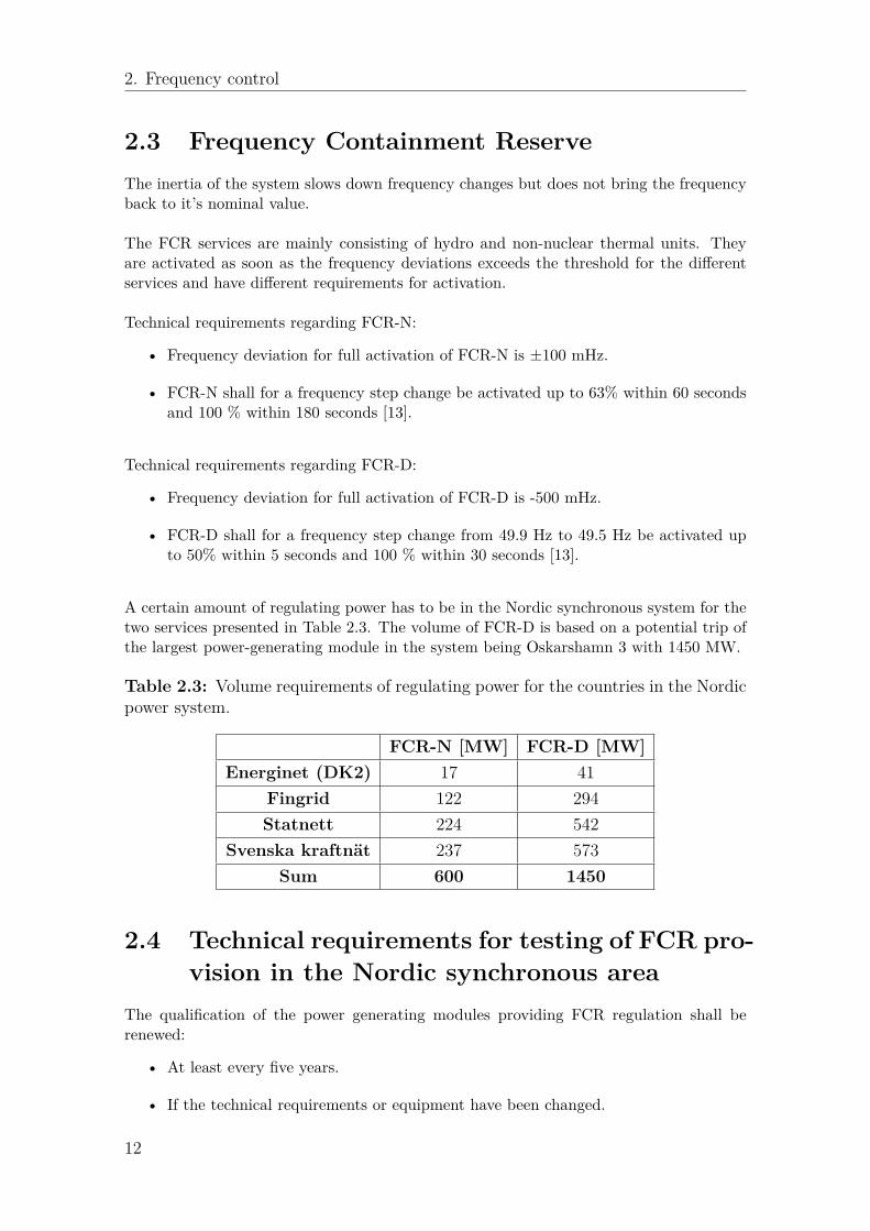
A certain amount of regulating power has to be in the Nordic synchronous system for thetwo services presented in Table 2.3. The volume of FCR-D is based on a potential trip ofthe largest power-generating module in the system being Oskarshamn 3 with 1450 MW.
Table 2.3: Volume requirements of regulating power for the countries in the Nordicpower system.
FCR-N [MW] FCR-D [MW]Energinet (DK2) 17 41
Fingrid 122 294Statnett 224 542
Svenska kraftnät 237 573Sum 600 1450
2.4 Technical requirements for testing of FCR pro-vision in the Nordic synchronous area
The qualification of the power generating modules providing FCR regulation shall berenewed:
• At least every five years.
• If the technical requirements or equipment have been changed.
12
2. Frequency control
• If the equipment regarding activation of FCR has been modernised [13].
The technical requirements for the testing unit are described in [14] and the logged datafile should as a minimum include the following list.
• Instantaneous active power in MW with a resolution of 0.01 MW and an accuracyof 0.5 % of the rated power of the providing entity, or better. The value shall besuch, that it covers all active power changes as a result of the FCR activation.
• Measured grid frequency in Hz, with a resolution of 1 mHz and an accuracy of 10mHz or better.
• Applied frequency signal, with a resolution of 1 mHz and an accuracy of 10 mHz orbetter.
• Status id indicating which controller parameter set is active, if it can be automati-cally changed during the test.
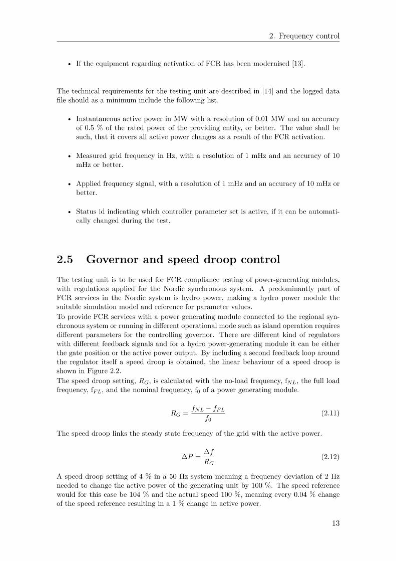
2.5 Governor and speed droop controlThe testing unit is to be used for FCR compliance testing of power-generating modules,with regulations applied for the Nordic synchronous system. A predominantly part ofFCR services in the Nordic system is hydro power, making a hydro power module thesuitable simulation model and reference for parameter values.To provide FCR services with a power generating module connected to the regional syn-chronous system or running in different operational mode such as island operation requiresdifferent parameters for the controlling governor. There are different kind of regulatorswith different feedback signals and for a hydro power-generating module it can be eitherthe gate position or the active power output. By including a second feedback loop aroundthe regulator itself a speed droop is obtained, the linear behaviour of a speed droop isshown in Figure 2.2.The speed droop setting, RG, is calculated with the no-load frequency, fNL, the full loadfrequency, fFL, and the nominal frequency, f0 of a power generating module.
RG = fNL − fFLf0
(2.11)
The speed droop links the steady state frequency of the grid with the active power.
∆P = ∆fRG
(2.12)
A speed droop setting of 4 % in a 50 Hz system meaning a frequency deviation of 2 Hzneeded to change the active power of the generating unit by 100 %. The speed referencewould for this case be 104 % and the actual speed 100 %, meaning every 0.04 % changeof the speed reference resulting in a 1 % change in active power.
13
2. Frequency control
Figure 2.2: Ideal steady-state characteristics of a governor with speed droop con-trol.
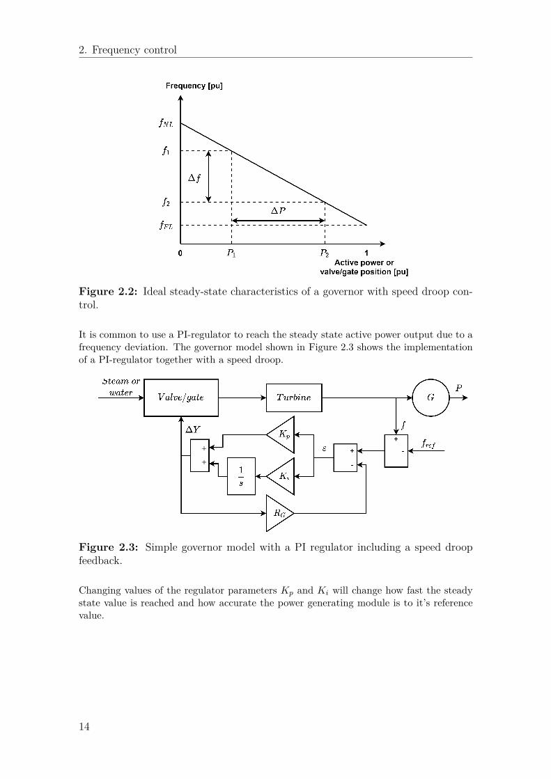
It is common to use a PI-regulator to reach the steady state active power output due to afrequency deviation. The governor model shown in Figure 2.3 shows the implementationof a PI-regulator together with a speed droop.
Figure 2.3: Simple governor model with a PI regulator including a speed droopfeedback.
Changing values of the regulator parameters Kp and Ki will change how fast the steadystate value is reached and how accurate the power generating module is to it’s referencevalue.
14

3Test principle
The principle of the testing procedure is to study the response of active power output ofpower-generating module due to a step of the frequency. This is done by replacing thenormal grid frequency feedback to the governor with a simulated frequency signal. Inorder to acquire the entire system response including the governor, the simulated signalis placed outside the governor shown in Figure 3.1 [15]. To obtain the active and reactivepower, the voltage and current are measured at the power-generating module’s terminal.The operational modes to be tested are a power-generating module in open loop and onein closed loop described in Section 3.1 and 3.2. The difference is that the frequency signalfor the open loop operation is based on a set value, while for the closed loop operation itis calculated from the measured active power of the power-generating module and a setvalue for the load in the system. The power-generating module will always be connectedto a strong grid and the response of a changing active power will be due to a changingcurrent.Using the testing unit to control a real power-generating module without verifying properfunctioning and performance of it would be unsafe, as the machine could reach criticaloperating limits. Therefore the development is first done in software and later realizedusing DACs, utilising the same principle described in Section 5.3. This method allowsfunction testing of the testing unit in close to ideal conditions while proceeding to adddelays and uncertainties in a safe manner.
15
3. Test principle
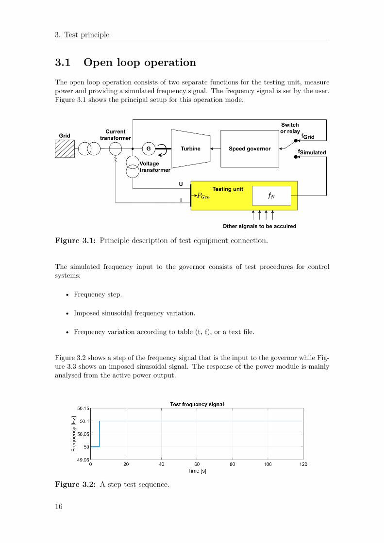
3.1 Open loop operationThe open loop operation consists of two separate functions for the testing unit, measurepower and providing a simulated frequency signal. The frequency signal is set by the user.Figure 3.1 shows the principal setup for this operation mode.
Figure 3.1: Principle description of test equipment connection.
The simulated frequency input to the governor consists of test procedures for controlsystems:
• Frequency step.
• Imposed sinusoidal frequency variation.
• Frequency variation according to table (t, f), or a text file.
Figure 3.2 shows a step of the frequency signal that is the input to the governor while Fig-ure 3.3 shows an imposed sinusoidal signal. The response of the power module is mainlyanalysed from the active power output.
Figure 3.2: A step test sequence.
16
3. Test principle
Figure 3.3: An imposed sinusoidal test sequence.
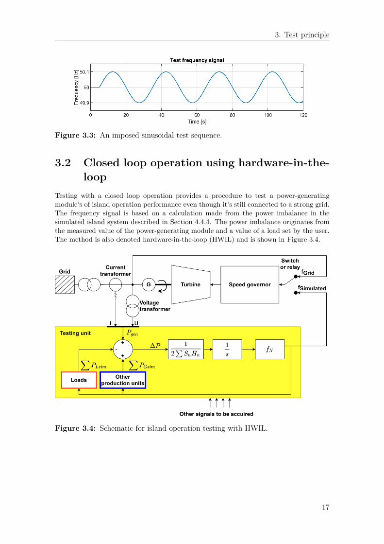
3.2 Closed loop operation using hardware-in-the-loop
Testing with a closed loop operation provides a procedure to test a power-generatingmodule’s of island operation performance even though it’s still connected to a strong grid.The frequency signal is based on a calculation made from the power imbalance in thesimulated island system described in Section 4.4.4. The power imbalance originates fromthe measured value of the power-generating module and a value of a load set by the user.The method is also denoted hardware-in-the-loop (HWIL) and is shown in Figure 3.4.
Figure 3.4: Schematic for island operation testing with HWIL.
17
3. Test principle
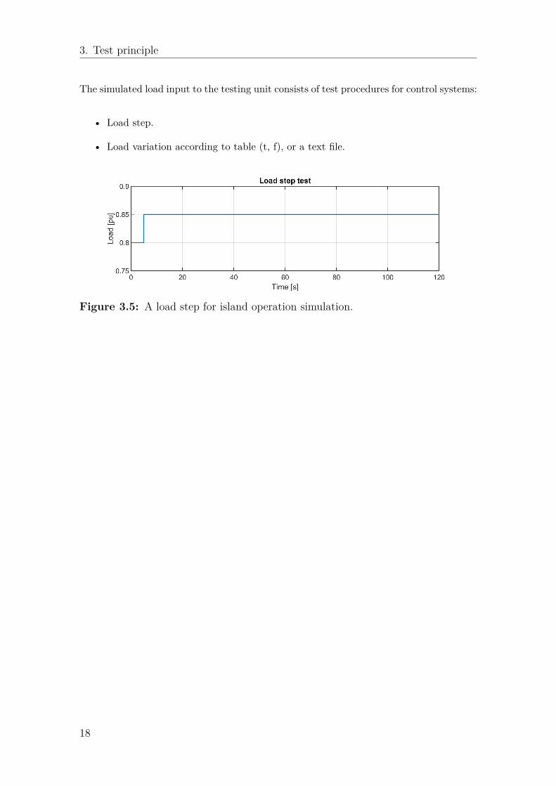
The simulated load input to the testing unit consists of test procedures for control systems:
• Load step.
• Load variation according to table (t, f), or a text file.
Figure 3.5: A load step for island operation simulation.
18

4Protrol’s testing unit
The hardware of the testing unit is Protrol’s already existing hardware for the productIPC4020 together with the expansion of a new PCB for the application.
4.1 HardwareThe testing unit holds two PCBs, one for current measurements, binary inputs, powersupply and auxiliary ports and the other with voltage measurements, analog inputs, binaryinputs and the DAC port. The two PCB:s are being run with two central processing units(CPUs) and a clock oscillator.
Table 4.1: Processors and clock oscillator of the testing unit.
Component DenotionMCPU STM32F765VIT6CPU STM32F413RGT6
Clock oscillator HXO-36A
The SRAM memory size of the MCPU is 512 Kbytes and the frequency stability of theclock oscillator is 3 ppm.
19
4. Protrol’s testing unit
The ports of the module are of a plug in type and described in Table 4.2 below.
Table 4.2: Ports of the testing unit.
Type of port Amount of ports Rating of port(s)Power supply 1 24-48 VDC
Current measurement 3 5 AVoltage measurement 4 110 VACL−N
Voltage measurement 8 10 VACL−N
Binary inputs 20 24-110 VDC
Binary outputs 4 Breaking capacity8 A at 250 VAC/30 VDC
Binary outputs 4 Breaking capacity5 A at 250 VAC/30 VDC
Analog voltage output 1 ±10 VAnalog current output 1 ± 20 mARJ45 communication 1 10/100 Base
USB type B 1 -
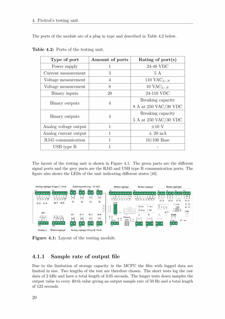
The layout of the testing unit is shown in Figure 4.1. The green parts are the differentsignal ports and the grey parts are the RJ45 and USB type B communication ports. Thefigure also shows the LEDs of the unit indicating different states [16].
Figure 4.1: Layout of the testing module.
4.1.1 Sample rate of output fileDue to the limitation of storage capacity in the MCPU the files with logged data arelimited in size. Two lengths of the test are therefore chosen. The short tests log the rawdata of 2 kHz and have a total length of 3.05 seconds. The longer tests down samples theoutput value to every 40:th value giving an output sample rate of 50 Hz and a total lengthof 122 seconds.
20

4. Protrol’s testing unit
4.2 Web interface
The web interface is reached through the RJ45 or USB connector and is used for monitoringthe unit real time or setting settings. The status of binary inputs and outputs, values ofmeasurements and the file with the logged data is reached through the web interface.
4.3 Software development tool
The drivers and implementation of the new hardware are already done and the imple-mentation of new code concerns handling of variables and signals. Atollic TrueSTUDIOis used as the C integrated development environment (IDE). It is an Eclipse based IDEmade for development with STM32 processors.
4.4 Signal processing and software implementa-tion
The testing unit’s main functionalities are:
• Measure active and reactive power in a circuit.
• Track the grid frequency.
• Provide a simulated frequency signal.
To do so a combination of a phase locked loop (PLL) and synchronous coordinates are usedtogether described in Section 4.4.3. The theory of them individually are first described inSection 4.4.1 and 4.4.2. They are based on the measurement of three phase voltages andcurrents.
4.4.1 Synchronous coordinates
To simplify analysis of three phase circuits, values are often transformed into the dq-frame.The benefit of having the vectors in this coordinate system is that they will appear as DCquantities in the corresponding reference frames and hence simplify calculations.
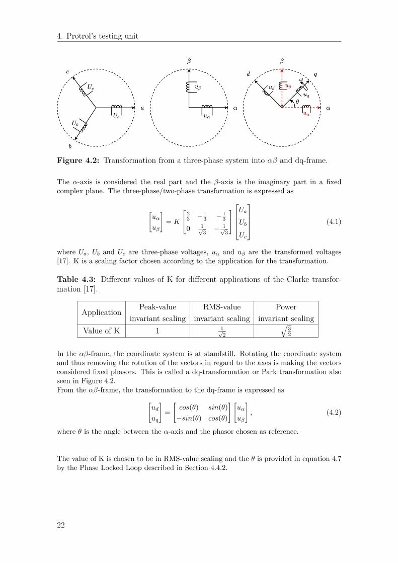
First the three phase values are transformed with a Clarke transformation into an equiv-alent two-phase system with two perpendicular axes, denoted α and β, shown in Figure4.2.
21
4. Protrol’s testing unit
Figure 4.2: Transformation from a three-phase system into αβ and dq-frame.
The α-axis is considered the real part and the β-axis is the imaginary part in a fixedcomplex plane. The three-phase/two-phase transformation is expressed as
[uα
uβ
]= K
23 −1
3 −13
0 1√3 − 1√
3
Ua
Ub
Uc
(4.1)
where Ua, Ub and Uc are three-phase voltages, uα and uβ are the transformed voltages[17]. K is a scaling factor chosen according to the application for the transformation.
Table 4.3: Different values of K for different applications of the Clarke transfor-mation [17].
Application Peak-valueinvariant scaling
RMS-valueinvariant scaling
Powerinvariant scaling
Value of K 1 1√2
√32
In the αβ-frame, the coordinate system is at standstill. Rotating the coordinate systemand thus removing the rotation of the vectors in regard to the axes is making the vectorsconsidered fixed phasors. This is called a dq-transformation or Park transformation alsoseen in Figure 4.2.From the αβ-frame, the transformation to the dq-frame is expressed as[
ud
uq
]=[cos(θ) sin(θ)−sin(θ) cos(θ)
] [uα
uβ
], (4.2)
where θ is the angle between the α-axis and the phasor chosen as reference.
The value of K is chosen to be in RMS-value scaling and the θ is provided in equation 4.7by the Phase Locked Loop described in Section 4.4.2.
22
4. Protrol’s testing unit
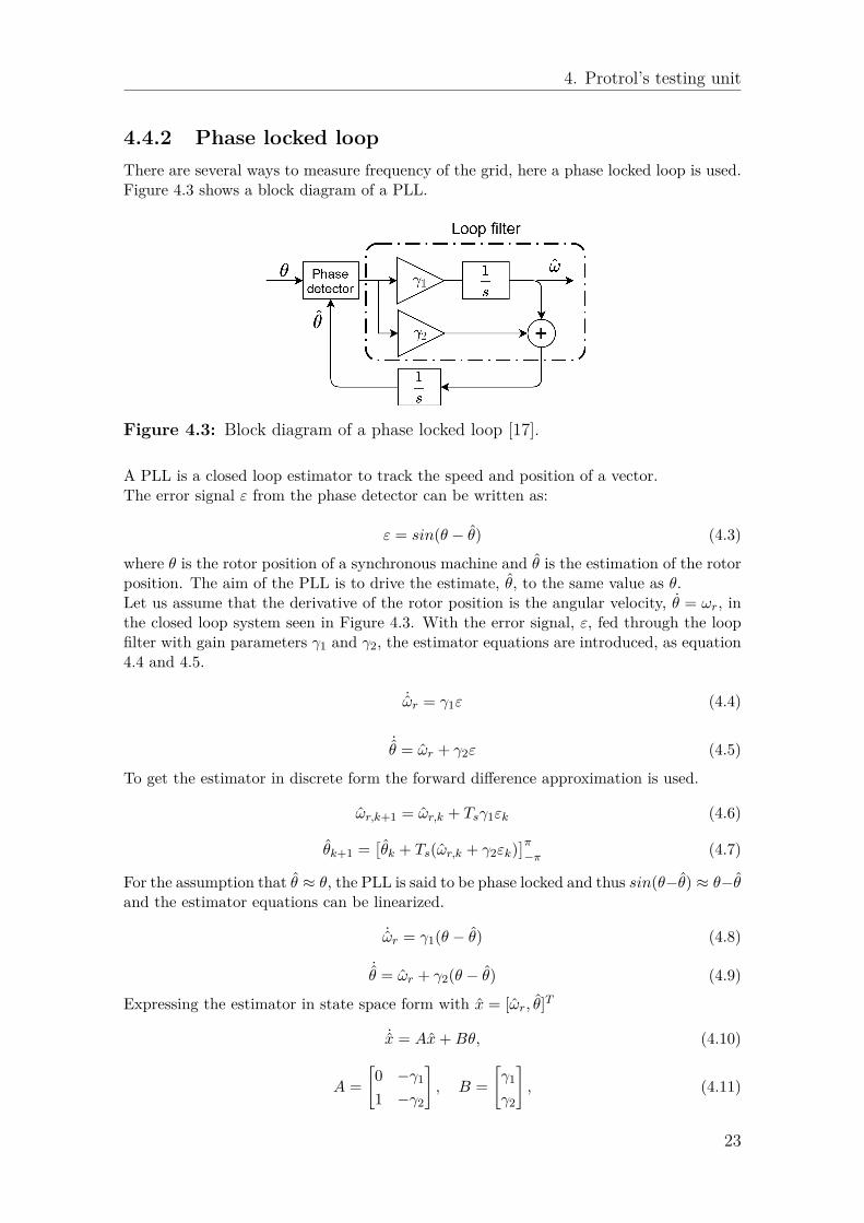
4.4.2 Phase locked loopThere are several ways to measure frequency of the grid, here a phase locked loop is used.Figure 4.3 shows a block diagram of a PLL.
Figure 4.3: Block diagram of a phase locked loop [17].
A PLL is a closed loop estimator to track the speed and position of a vector.The error signal ε from the phase detector can be written as:
ε = sin(θ − θ) (4.3)
where θ is the rotor position of a synchronous machine and θ is the estimation of the rotorposition. The aim of the PLL is to drive the estimate, θ, to the same value as θ.Let us assume that the derivative of the rotor position is the angular velocity, θ = ωr, inthe closed loop system seen in Figure 4.3. With the error signal, ε, fed through the loopfilter with gain parameters γ1 and γ2, the estimator equations are introduced, as equation4.4 and 4.5.
˙ωr = γ1ε (4.4)
˙θ = ωr + γ2ε (4.5)
To get the estimator in discrete form the forward difference approximation is used.
ωr,k+1 = ωr,k + Tsγ1εk (4.6)
θk+1 =[θk + Ts(ωr,k + γ2εk)
]π−π (4.7)
For the assumption that θ ≈ θ, the PLL is said to be phase locked and thus sin(θ−θ) ≈ θ−θand the estimator equations can be linearized.
˙ωr = γ1(θ − θ) (4.8)
˙θ = ωr + γ2(θ − θ) (4.9)
Expressing the estimator in state space form with x = [ωr, θ]T
˙x = Ax+Bθ, (4.10)
A =[0 −γ1
1 −γ2
], B =
[γ1
γ2
], (4.11)
23
4. Protrol’s testing unit
gives the poles by the characteristic polynomial
det(sI −A) = s2 + γ2s+ γ1. (4.12)
The poles can be chosen from the characteristic polynomial
(s+ ρ)2 = s2 + 2ρs+ ρ2 → γ1 = ρ2, γ2 = 2ρ (4.13)
where ρ is considered the bandwidth of the estimator.To keep a stable system performance of a closed loop system and have a precise forwarddifference approximation, the recommendation is to select the angular sampling frequency,ωs, at least 10 times higher than the closed loop bandwidth, ρ.
ωs ≥ 10 · ρ (4.14)
Where ωs comes from the sampling frequency fs.
ωs = 2πfs (4.15)
According to [18] the transfer function from ε to θ can be described as below, if the systemis considered linear and time-invariant.
GPLL(z) = z2ρTs + ρTs(ρTs − 2)z2 + z2(ρTs − 1) + ρTs(ρTs − 2) + 1 (4.16)
Where Ts is the sampling time.
Ts = 1fs
(4.17)
In case of an unsymmetrical grid, the dq-transformed signals described in Section 4.4.1,will contain a negative sequence voltage. The negative sequence component will occur asan oscillation of twice the grid frequency in the dq-frame. For the procedure describedin Section 4.4.3 where the uq phasor is the input signal to the PLL, the choice of a lowbandwidth can filter this oscillation out [18].
The parameters chosen in the PLL are:
Table 4.4: Parameter selection for the PLL.
Parameter fs ρ
Value 2000 31.4
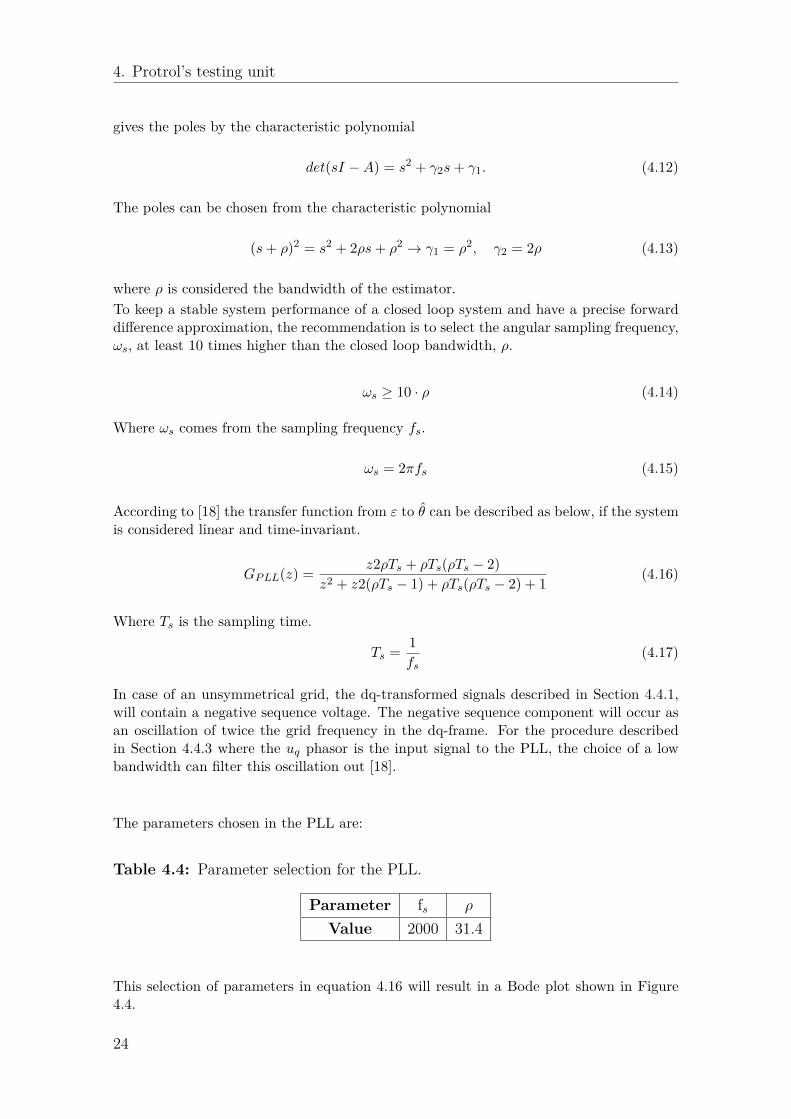
This selection of parameters in equation 4.16 will result in a Bode plot shown in Figure4.4.
24
4. Protrol’s testing unit
Figure 4.4: Bode plot of the PLL described in Section 4.4.2.
A 100 Hz oscillation in the uq phasor coming from a negative sequence voltage will thenbe filtered out -20 dB or 90%.
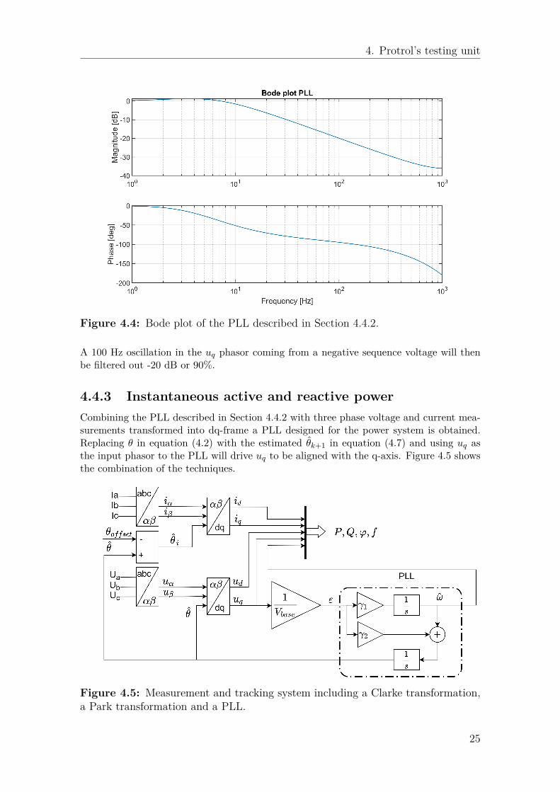
4.4.3 Instantaneous active and reactive powerCombining the PLL described in Section 4.4.2 with three phase voltage and current mea-surements transformed into dq-frame a PLL designed for the power system is obtained.Replacing θ in equation (4.2) with the estimated θk+1 in equation (4.7) and using uq asthe input phasor to the PLL will drive uq to be aligned with the q-axis. Figure 4.5 showsthe combination of the techniques.
Figure 4.5: Measurement and tracking system including a Clarke transformation,a Park transformation and a PLL.
25
4. Protrol’s testing unit
To calculate the active power, P , reactive power, Q, and the phase difference betweenvoltage and current, ϕ, measured currents also needs to be in the dq-frame as id and iq[17]. P, Q and ϕ is then calculated with
P = 32K2 (ud · id + uq · iq), (4.18)
Q = 32K2 (uq · id − ud · iq), (4.19)
ϕ = arctan(QP
). (4.20)
For calibration purposes θk+1,i in the Park transformation can be adjusted from θk+1 withθoffset.
θk+1,i = θk+1 − θoffset (4.21)
This offset is due to phase shift properties in transformers and hardware filters in the mea-suring equipment creating a phase shift between the voltage and the current. The abilityto calibrate the system is then possible with measuring voltage and current in a fully resis-tive circuit having θoffset set to zero and calculating ϕ. The value of ϕ is then set to θoffset.
The frequency in the circuit is calculated from the estimated speed ωr,k+1 in the PLL.
f = ωr,k+12π (4.22)
4.4.4 Island operation and closed loop simulationIsland operation refers to a power network running in isolation from the national grid.It consists of at least one power module or HVDC link supplying power to this network,controlling the frequency and voltage.To test a power-generating module’s performance of island operation frequency controlthe methodology in Section 3.2 is used. The frequency in the system is calculated basedon the knowledge of the kinetic energy, Wk, the active power input,
∑PGsim of other
power-generating module(s) and a simulated load curve∑PLsim. With the measured
active power, PGen, the power imbalance is calculated.
∆P = Pgen −∑
PLsim −∑
PGsim (4.23)
To describe the Rate-of-Change-of-Frequency (RoCoF) equation (2.10) is used in discreteform.
dfN
dt=
∆P · fN2 ·∑Mn=1 Sn ·Hn
(4.24)
whereM is the amount of units and Sn andHn are the rated power and the inertia constantof the unit(s). The difference in frequency is based on the sample time Ts between thetwo samples N and N + 1.
∆fN+1 =dfN
dt· Ts (4.25)
And the new frequency fN+1 is calculated.
fN+1 = fN + ∆fN+1 (4.26)
26
4. Protrol’s testing unit
4.4.5 Discrete time low pass filterTo smooth out a high frequent or random noise in a measurement signal it’s common touse a first order filter. To derive a filter with the backward differentiation method theLaplace transform transfer function is described as
H(s) = y(s)u(s) = 1
Tfs+ 1 . (4.27)
Where Tf is the time-constant, u the filter input and y the filter output. Rewriting (4.27)gives
Tfs · y(s) + y(s) = u(s). (4.28)
Taking the Laplace transform of both sides of equation (4.28) gives the following differentialequation.
Tf y(t) + y(t) = u(t) (4.29)
which in discrete form where tk is considered a point in time is written as
Tf y(tk) + y(tk) = u(tk) (4.30)
The derivative is approximated with the backward differentiation method seen below
y(tk) ≈y(tk)− y(tk−1)
h(4.31)
where h is the sample time or step size. Combining equation (4.30) and (4.31) then gives
Tfy(tk)− y(tk−1)
h+ y(tk) = u(tk). (4.32)
Solving for y(tk) gives
y(tk) = TfTf + h
y(tk−1) + h
Tf + hu(tk) (4.33)
and can be written asy(tk) = (1− a)y(tk−1) + au(tk), (4.34)
where the filter parameter usually is written as
a = h
Tf + h. (4.35)
27

4. Protrol’s testing unit
28
5Performance testing
To validate and get the performance of the testing unit, the implemented code is simulatedin ideal conditions and the hardware is tested with voltages and currents with a lowharmonic content. The last test is a combination of both, where a simulation of a hydropower-generating module is controlled and measured with the testing unit. The goal isto acquire limitations in the implemented code described but also hardware related issuessuch as delays and noise in the testing unit.
5.1 Measuring precisionTo test the precision in the measurements the relay testers described in Section 5.1.1 areused. A predefined sequence is provided to the testing unit changing the voltage leveland frequency. This gives a way of testing the response time and precision of the PLLand instantaneous power described in Section 4.4.3. Figure 5.1 shows the setup of themeasurement.
Figure 5.1: Test setup with relay tester ONLLY-M783 and OMICRON CMC 356.Dotted lines are operations made in software and full lines are physical cables.
The logging of the testing unit is activated with a binary input. The sequence of the relaytester is then matched to the length of the output file described in Section 4.1.1.The calibration of the voltage measurement is done with giving out a direct current (DC)voltage and adjusting the output to the real value.The voltage is kept at 10 VL−N , i.e. VBase=10 V.
29
5. Performance testing
5.1.1 ONLLY-AT633 and OMICRON CMC 356ONLLY-AT633 and OMICRON CMC 356 are both relay test units and commissioningtools able to send out both voltages, currents and binary signals on separate channels.They can be programmed to send out predefined sequences where the voltage, current,frequency and binary outputs are controlled over time. Below are the technical specifica-tions.
Table 5.1: ONLLY-AT633 technical specification.
Type of port Nr. of ports Rating Accuracy
Current output 3 35 A <4 mA absolute<0.2 % relative
Voltage output 3 125 V <4 mV absolute<0.29 % relative
Frequency - 10-1000 Hz 10 Hz <f <65 Hznot more than +0.001 Hz
Table 5.2: OMICRON CMC 356 technical specification.
Type Nr. of ports Rating AccuracyCurrent output 6 32 A <0.05% reading + 0.02% rangeVoltage output 4 400 V <0.03% reading + 0.01 % range
Binary output 4 6.67 A at 300 VAC
0.17 A at 300 VDC
-
Binary input 10 20-300 V -
Frequency - 10-1000 Hz ± 0.5 ppm± 1 ppm drift
30
5. Performance testing
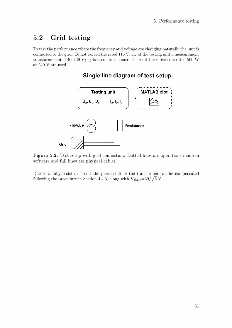
5.2 Grid testingTo test the performance where the frequency and voltage are changing naturally the unit isconnected to the grid. To not exceed the rated 115 VL−N of the testing unit a measurementtransformer rated 400/39 VL−L is used. In the current circuit three resistors rated 500 Wat 240 V are used.
Figure 5.2: Test setup with grid connection. Dotted lines are operations made insoftware and full lines are physical cables.
Due to a fully resistive circuit the phase shift of the transformer can be compensatedfollowing the procedure in Section 4.4.3, along with VBase=39/
√3 V.
31
5. Performance testing
5.3 Application testing
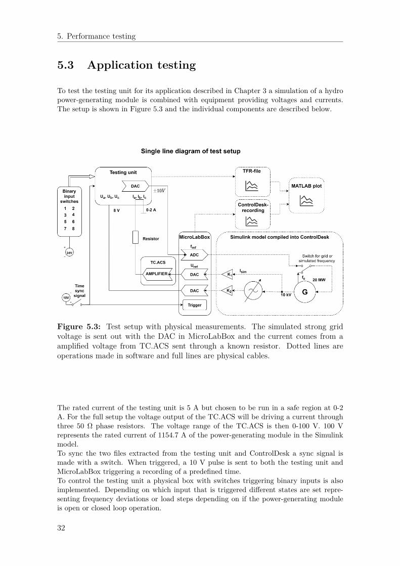
To test the testing unit for its application described in Chapter 3 a simulation of a hydropower-generating module is combined with equipment providing voltages and currents.The setup is shown in Figure 5.3 and the individual components are described below.
Figure 5.3: Test setup with physical measurements. The simulated strong gridvoltage is sent out with the DAC in MicroLabBox and the current comes from aamplified voltage from TC.ACS sent through a known resistor. Dotted lines areoperations made in software and full lines are physical cables.
The rated current of the testing unit is 5 A but chosen to be run in a safe region at 0-2A. For the full setup the voltage output of the TC.ACS will be driving a current throughthree 50 Ω phase resistors. The voltage range of the TC.ACS is then 0-100 V. 100 Vrepresents the rated current of 1154.7 A of the power-generating module in the Simulinkmodel.To sync the two files extracted from the testing unit and ControlDesk a sync signal ismade with a switch. When triggered, a 10 V pulse is sent to both the testing unit andMicroLabBox triggering a recording of a predefined time.To control the testing unit a physical box with switches triggering binary inputs is alsoimplemented. Depending on which input that is triggered different states are set repre-senting frequency deviations or load steps depending on if the power-generating moduleis open or closed loop operation.
32
5. Performance testing
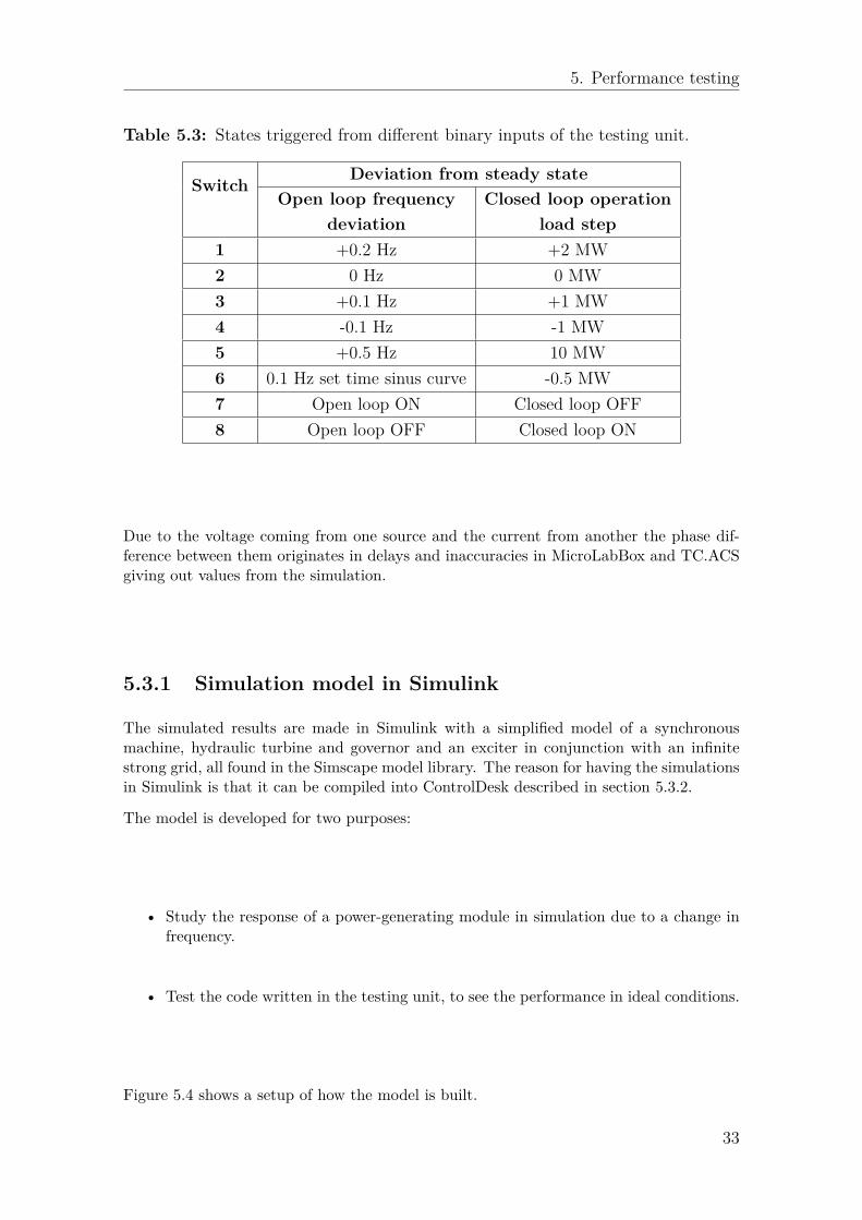
Table 5.3: States triggered from different binary inputs of the testing unit.
Switch Deviation from steady stateOpen loop frequency
deviationClosed loop operation
load step1 +0.2 Hz +2 MW2 0 Hz 0 MW3 +0.1 Hz +1 MW4 -0.1 Hz -1 MW5 +0.5 Hz 10 MW6 0.1 Hz set time sinus curve -0.5 MW7 Open loop ON Closed loop OFF8 Open loop OFF Closed loop ON
Due to the voltage coming from one source and the current from another the phase dif-ference between them originates in delays and inaccuracies in MicroLabBox and TC.ACSgiving out values from the simulation.
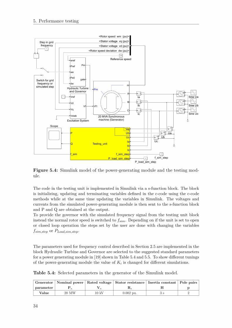
5.3.1 Simulation model in Simulink
The simulated results are made in Simulink with a simplified model of a synchronousmachine, hydraulic turbine and governor and an exciter in conjunction with an infinitestrong grid, all found in the Simscape model library. The reason for having the simulationsin Simulink is that it can be compiled into ControlDesk described in section 5.3.2.
The model is developed for two purposes:
• Study the response of a power-generating module in simulation due to a change infrequency.
• Test the code written in the testing unit, to see the performance in ideal conditions.
Figure 5.4 shows a setup of how the model is built.
33
5. Performance testing
Figure 5.4: Simulink model of the power-generating module and the testing mod-ule.
The code in the testing unit is implemented in Simulink via a s-function block. The blockis initializing, updating and terminating variables defined in the c-code using the c-codemethods while at the same time updating the variables in Simulink. The voltages andcurrents from the simulated power-generating module is then sent to the s-function blockand P and Q are obtained at the output.To provide the governor with the simulated frequency signal from the testing unit blockinstead the normal rotor speed is switched to fsim. Depending on if the unit is set to openor closed loop operation the steps set by the user are done with changing the variablesfsim,step or PLoad,sim,step.
The parameters used for frequency control described in Section 2.5 are implemented in theblock Hydraulic Turbine and Governor are selected to the suggested standard parametersfor a power generating module in [19] shown in Table 5.4 and 5.5. To show different tuningsof the power-generating module the value of Ki is changed for different simulations.
Table 5.4: Selected parameters in the generator of the Simulink model.
Generatorparameter
Nominal power Rated voltage Stator resistance Inertia constant Pole pairsPn Vn Rs H p
Value 20 MW 10 kV 0.002 pu. 3 s 2
34
5. Performance testing
Table 5.5: Selected parameters in the governor of the Simulink model.
Governorparameter
Permanent Droop ProportionalIntegratorOpen loop
IntegratorClosed loop
Droopreference
RG Kp Ki Ki
Value 4% 2.5 0.7 0.07 Gate position
The steady state active power of the power-generating module in the Simulink model isset to be 0.8 pu.
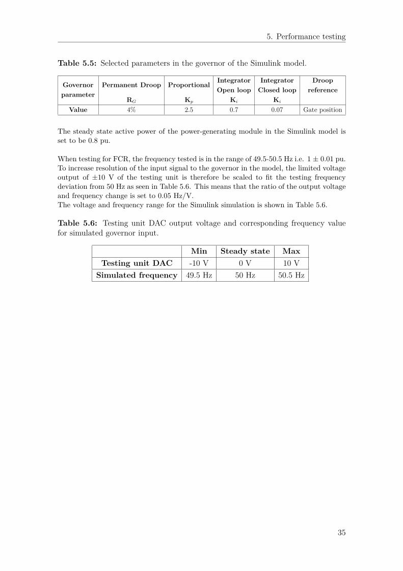
When testing for FCR, the frequency tested is in the range of 49.5-50.5 Hz i.e. 1 ± 0.01 pu.To increase resolution of the input signal to the governor in the model, the limited voltageoutput of ±10 V of the testing unit is therefore be scaled to fit the testing frequencydeviation from 50 Hz as seen in Table 5.6. This means that the ratio of the output voltageand frequency change is set to 0.05 Hz/V.The voltage and frequency range for the Simulink simulation is shown in Table 5.6.
Table 5.6: Testing unit DAC output voltage and corresponding frequency valuefor simulated governor input.
Min Steady state MaxTesting unit DAC -10 V 0 V 10 V
Simulated frequency 49.5 Hz 50 Hz 50.5 Hz
35
5. Performance testing
5.3.2 Simulation environment and software to hardware in-terface
To get a real-time-interface and measurable analog voltage signals ControlDesk and Mi-croLabBox from dSPACE are used. MicroLabBox is an electronic control unit (ECU) andControlDesk its instrumentation software.The MicroLabBox has 16 analog output cannels and 8 analog input channels with a voltagerange of ± 10 V all provided with a BNC-connector. The 10kV voltage and ∼ 1.6 kAcurrent that the power-generating module is being run at in steady state needs to bescaled down to fit the hardware. The Simulink model also needs to be modified withcertain dSPACE DAC and analog-to-digital converter (ADC) blocks, for communicationthe hardware. It is then compiled into ControlDesk where all the variables are monitoredand controlled.The testing unit samples data at a rate of 2 kHz and the MicroLabBox is set to a samplingrate of 20 kHz. The reason is to have better accuracy and higher resolution of the realtime simulations processed in ControlDesk. For the comparison of the results every 10:thsample of the ControlDesk-file is compared to the one from the testing unit.
5.3.3 Amplifier equipmentThe TC.ACS by REGATRON is a multi-level inverter acting as a full 4 quadrant 3-phasealternating current (AC) power source. Running it in amplifier mode and connecting theoutputs from the MicroLabBox to TC.ACS will amplify the voltage to the desired value.The technical specification of the TC.ACS is presented in Table 5.7.
Table 5.7: TC.ACS technical specification.
Type Rating AccuracyVoltage at 50/60 Hz - 0.05% FS
Voltage output 0-300 Vrms,L−N <1.5 VPhase angle - 1°Frequency 0-1000 Hz 2 mHz
36
6Results
This chapter contains the results of simulations and measurements, recorded simultaneousfor every test case, in graphs for different operation modes and control signals.
6.1 Precision testsThis section contains results from tests described in Section 5.1, performed to verify theprecision of the testing unit’s measurements.
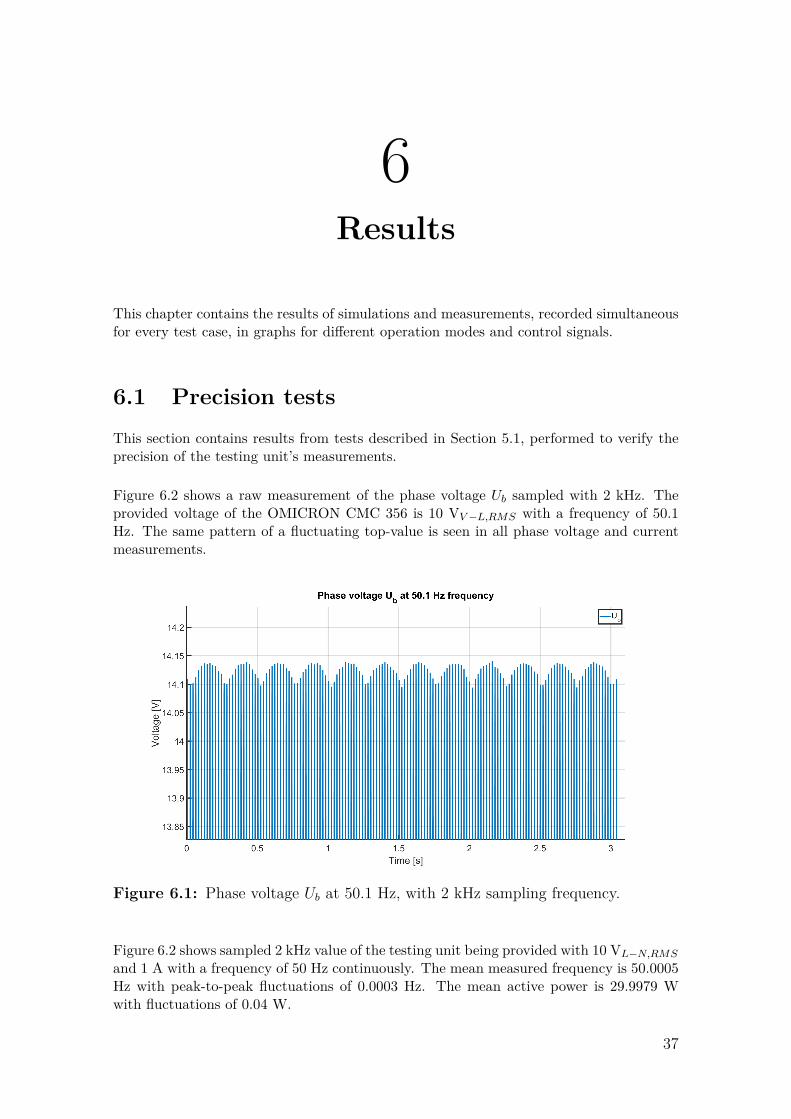
Figure 6.2 shows a raw measurement of the phase voltage Ub sampled with 2 kHz. Theprovided voltage of the OMICRON CMC 356 is 10 VV−L,RMS with a frequency of 50.1Hz. The same pattern of a fluctuating top-value is seen in all phase voltage and currentmeasurements.
Figure 6.1: Phase voltage Ub at 50.1 Hz, with 2 kHz sampling frequency.
Figure 6.2 shows sampled 2 kHz value of the testing unit being provided with 10 VL−N,RMS
and 1 A with a frequency of 50 Hz continuously. The mean measured frequency is 50.0005Hz with peak-to-peak fluctuations of 0.0003 Hz. The mean active power is 29.9979 Wwith fluctuations of 0.04 W.
37
6. Results
Figure 6.2: Active power and frequency sampled at 2 kHz.
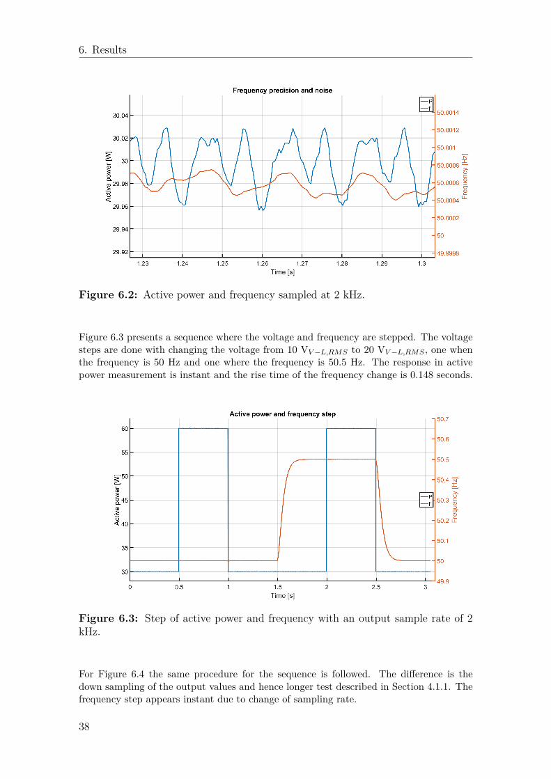
Figure 6.3 presents a sequence where the voltage and frequency are stepped. The voltagesteps are done with changing the voltage from 10 VV−L,RMS to 20 VV−L,RMS , one whenthe frequency is 50 Hz and one where the frequency is 50.5 Hz. The response in activepower measurement is instant and the rise time of the frequency change is 0.148 seconds.
Figure 6.3: Step of active power and frequency with an output sample rate of 2kHz.
For Figure 6.4 the same procedure for the sequence is followed. The difference is thedown sampling of the output values and hence longer test described in Section 4.1.1. Thefrequency step appears instant due to change of sampling rate.
38

6. Results
Figure 6.4: Step of active power and frequency with an output sample rate of 50Hz.
Looking closely at the active power when the frequency is 50.5 Hz shows small fluctuationsbut not when the frequency is at 50 Hz.
As soon as the frequency deviates from 50 Hz the magnitude of the voltage and currentmeasurements fluctuates for the long tests. The fluctuation appears to be linear with thedeviation from the nominal frequency, ∆f , and have the same pattern as the noise shownin Figure 6.2. Figure 6.5 shows a close up of the fluctuation, for a ∆f of 0.005 Hz and 0.1Hz.
Figure 6.5: Active power at frequencies of 50.005 Hz and 50.1 Hz consecutively,sampled at 2 kHz and then being down-sampled to 50 Hz.
39
6. Results
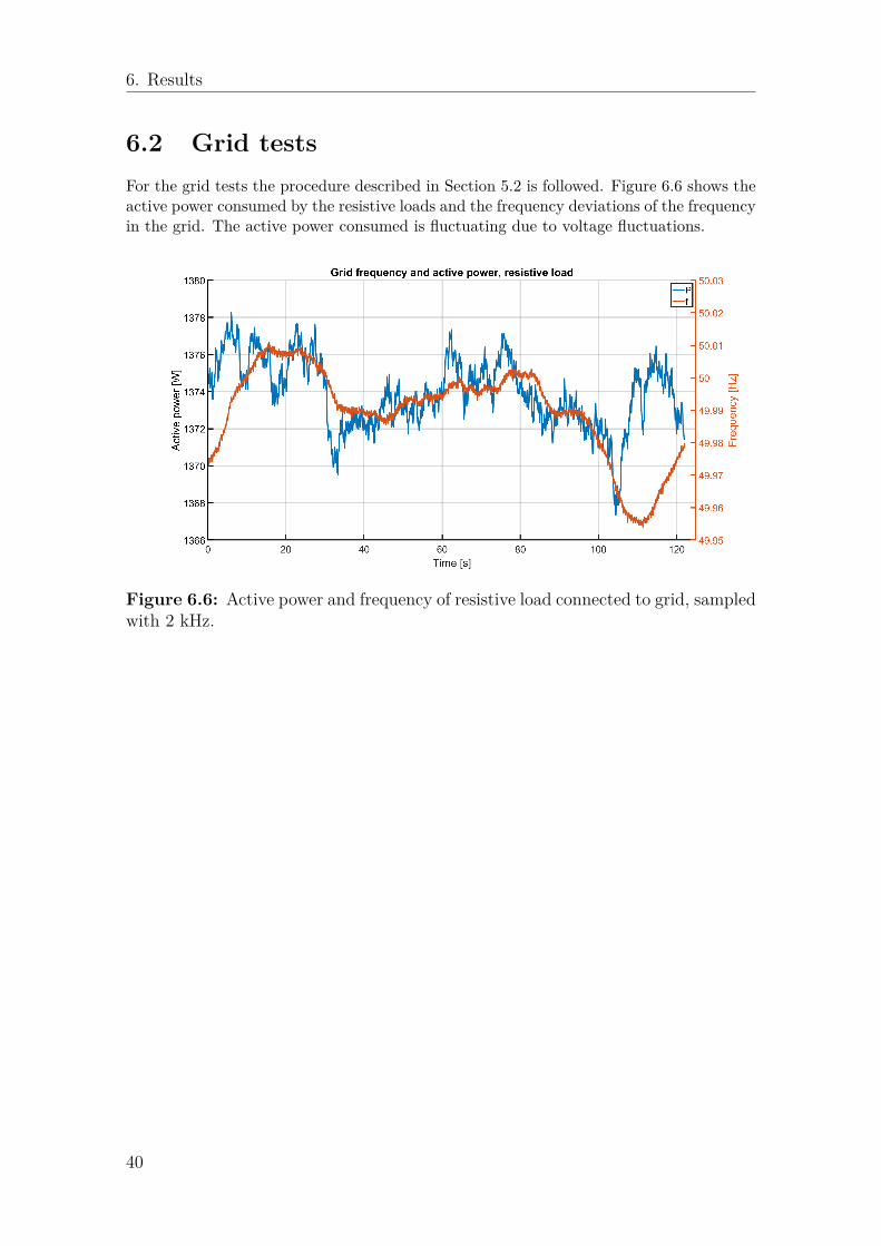
6.2 Grid testsFor the grid tests the procedure described in Section 5.2 is followed. Figure 6.6 shows theactive power consumed by the resistive loads and the frequency deviations of the frequencyin the grid. The active power consumed is fluctuating due to voltage fluctuations.
Figure 6.6: Active power and frequency of resistive load connected to grid, sampledwith 2 kHz.
40
6. Results
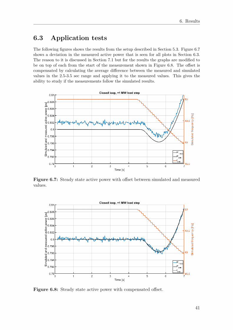
6.3 Application testsThe following figures shows the results from the setup described in Section 5.3. Figure 6.7shows a deviation in the measured active power that is seen for all plots in Section 6.3.The reason to it is discussed in Section 7.1 but for the results the graphs are modified tobe on top of each from the start of the measurement shown in Figure 6.8. The offset iscompensated by calculating the average difference between the measured and simulatedvalues in the 2.5-3.5 sec range and applying it to the measured values. This gives theability to study if the measurements follow the simulated results.
Figure 6.7: Steady state active power with offset between simulated and measuredvalues.
Figure 6.8: Steady state active power with compensated offset.
41
6. Results
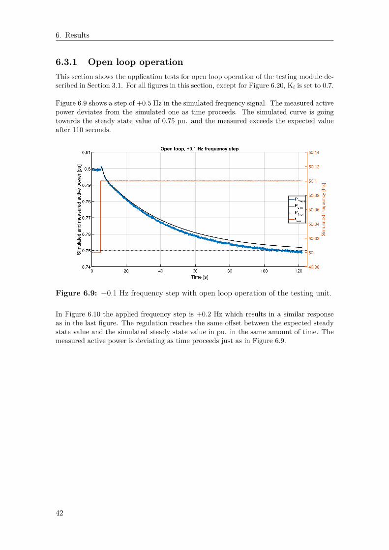
6.3.1 Open loop operationThis section shows the application tests for open loop operation of the testing module de-scribed in Section 3.1. For all figures in this section, except for Figure 6.20, Ki is set to 0.7.
Figure 6.9 shows a step of +0.5 Hz in the simulated frequency signal. The measured activepower deviates from the simulated one as time proceeds. The simulated curve is goingtowards the steady state value of 0.75 pu. and the measured exceeds the expected valueafter 110 seconds.
Figure 6.9: +0.1 Hz frequency step with open loop operation of the testing unit.
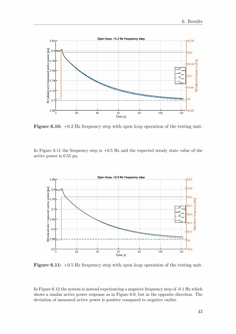
In Figure 6.10 the applied frequency step is +0.2 Hz which results in a similar responseas in the last figure. The regulation reaches the same offset between the expected steadystate value and the simulated steady state value in pu. in the same amount of time. Themeasured active power is deviating as time proceeds just as in Figure 6.9.
42
6. Results
Figure 6.10: +0.2 Hz frequency step with open loop operation of the testing unit.
In Figure 6.11 the frequency step is +0.5 Hz and the expected steady state value of theactive power is 0.55 pu.
Figure 6.11: +0.5 Hz frequency step with open loop operation of the testing unit.
In Figure 6.12 the system is instead experiencing a negative frequency step of -0.1 Hz whichshows a similar active power response as in Figure 6.9, but in the opposite direction. Thedeviation of measured active power is positive compared to negative earlier.
43
6. Results
Figure 6.12: -0.1 Hz frequency step with open loop operation of the testing unit.
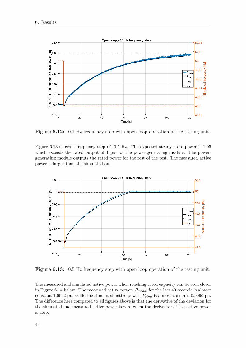
Figure 6.13 shows a frequency step of -0.5 Hz. The expected steady state power is 1.05which exceeds the rated output of 1 pu. of the power-generating module. The power-generating module outputs the rated power for the rest of the test. The measured activepower is larger than the simulated on.
Figure 6.13: -0.5 Hz frequency step with open loop operation of the testing unit.
The measured and simulated active power when reaching rated capacity can be seen closerin Figure 6.14 below. The measured active power, Pmeas, for the last 40 seconds is almostconstant 1.0042 pu, while the simulated active power, Psim, is almost constant 0.9990 pu.The difference here compared to all figures above is that the derivative of the deviation forthe simulated and measured active power is zero when the derivative of the active poweris zero.
44
6. Results
Figure 6.14: -0.5 Hz frequency step with open loop operation of the testing unitafter reaching maximum capacity.
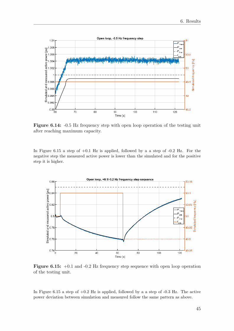
In Figure 6.15 a step of +0.1 Hz is applied, followed by a a step of -0.2 Hz. For thenegative step the measured active power is lower than the simulated and for the positivestep it is higher.
Figure 6.15: +0.1 and -0.2 Hz frequency step sequence with open loop operationof the testing unit.
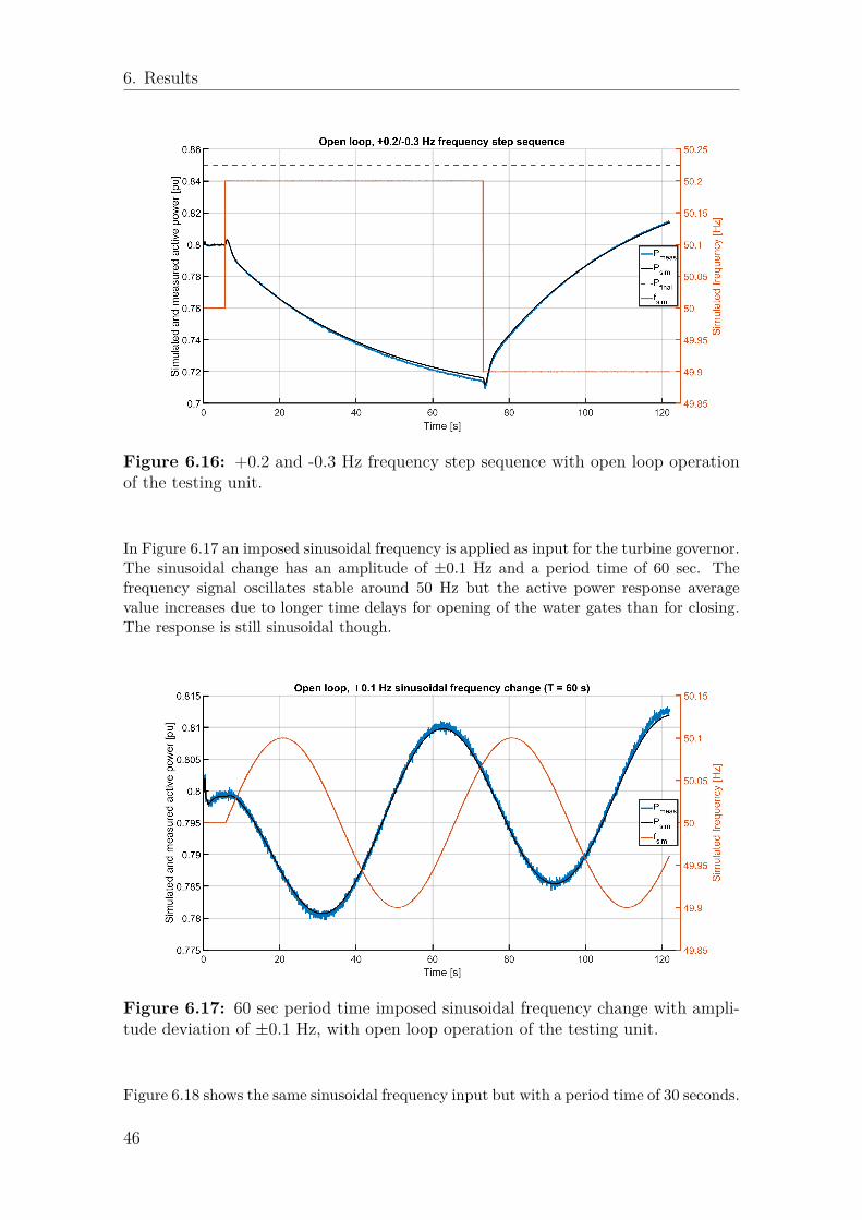
In Figure 6.15 a step of +0.2 Hz is applied, followed by a a step of -0.3 Hz. The activepower deviation between simulation and measured follow the same pattern as above.
45
6. Results
Figure 6.16: +0.2 and -0.3 Hz frequency step sequence with open loop operationof the testing unit.
In Figure 6.17 an imposed sinusoidal frequency is applied as input for the turbine governor.The sinusoidal change has an amplitude of ±0.1 Hz and a period time of 60 sec. Thefrequency signal oscillates stable around 50 Hz but the active power response averagevalue increases due to longer time delays for opening of the water gates than for closing.The response is still sinusoidal though.
Figure 6.17: 60 sec period time imposed sinusoidal frequency change with ampli-tude deviation of ±0.1 Hz, with open loop operation of the testing unit.
Figure 6.18 shows the same sinusoidal frequency input but with a period time of 30 seconds.
46
6. Results
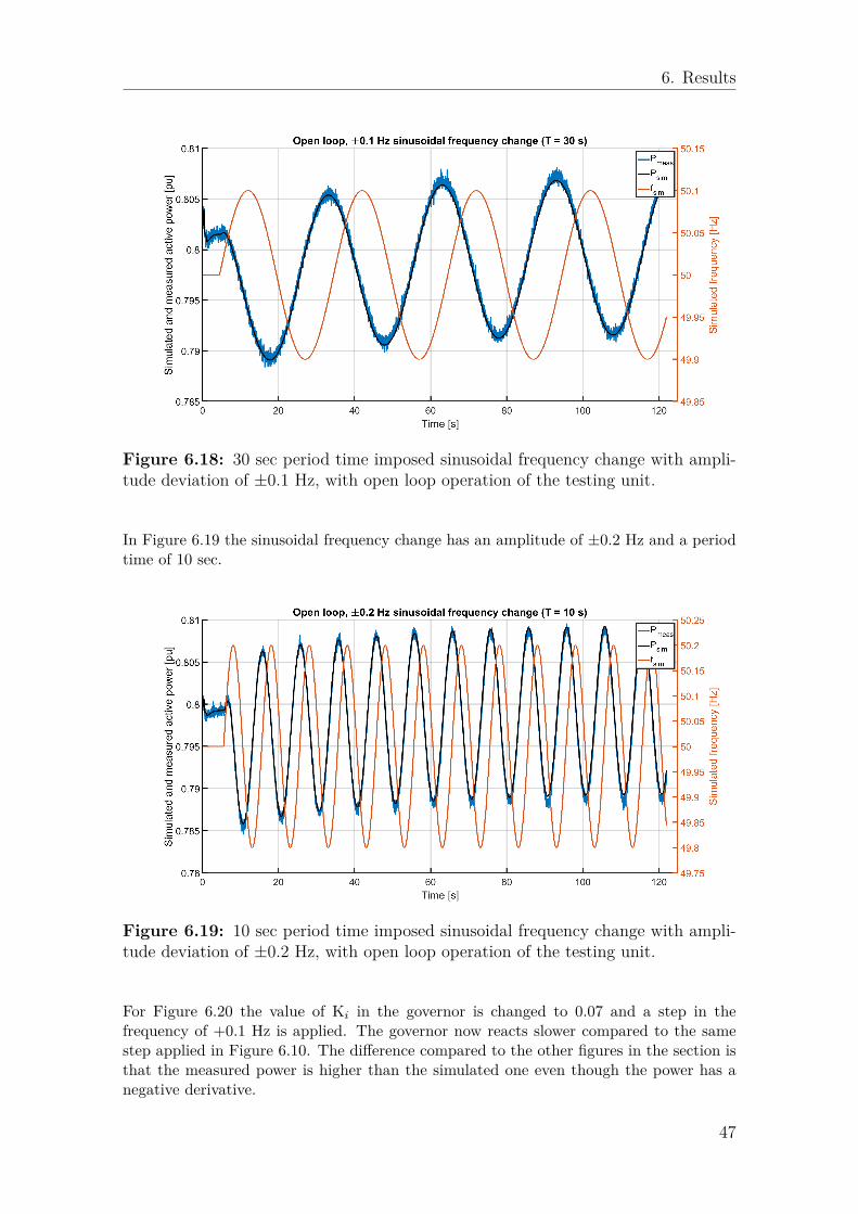
Figure 6.18: 30 sec period time imposed sinusoidal frequency change with ampli-tude deviation of ±0.1 Hz, with open loop operation of the testing unit.
In Figure 6.19 the sinusoidal frequency change has an amplitude of ±0.2 Hz and a periodtime of 10 sec.
Figure 6.19: 10 sec period time imposed sinusoidal frequency change with ampli-tude deviation of ±0.2 Hz, with open loop operation of the testing unit.
For Figure 6.20 the value of Ki in the governor is changed to 0.07 and a step in thefrequency of +0.1 Hz is applied. The governor now reacts slower compared to the samestep applied in Figure 6.10. The difference compared to the other figures in the section isthat the measured power is higher than the simulated one even though the power has anegative derivative.
47

6. Results
Figure 6.20: +0.1 Hz frequency step with open loop operation of the testing unitwith governor parameter Ki set to 0.07.
6.3.2 Closed loop operationThis section shows the application tests for closed loop operation of the testing moduledescribed in Section 3.2. The value of Ki is kept at 0.07.
Figure 6.21 shows the response for a load step of -1 MW. Notice the simulated frequencycalculation in the orange line. The expected steady state value is 0.75 pu. and the power-generating module reaches it after 22 seconds.
Figure 6.21: -1 MW load step with closed loop operation of the testing unit.
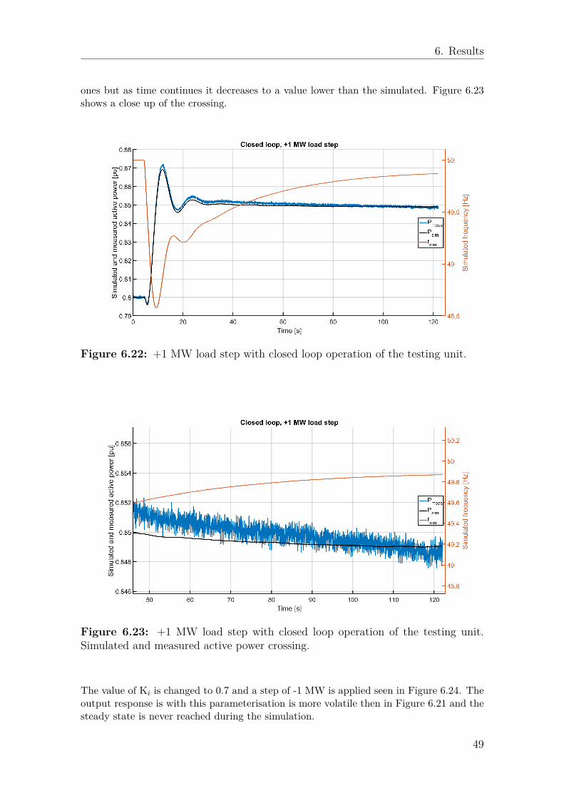
Figure 6.22 shows a load step of +1 MW and the result is similar to the previous one.The measured power is at the start of the steady state value higher than the simulated
48
6. Results
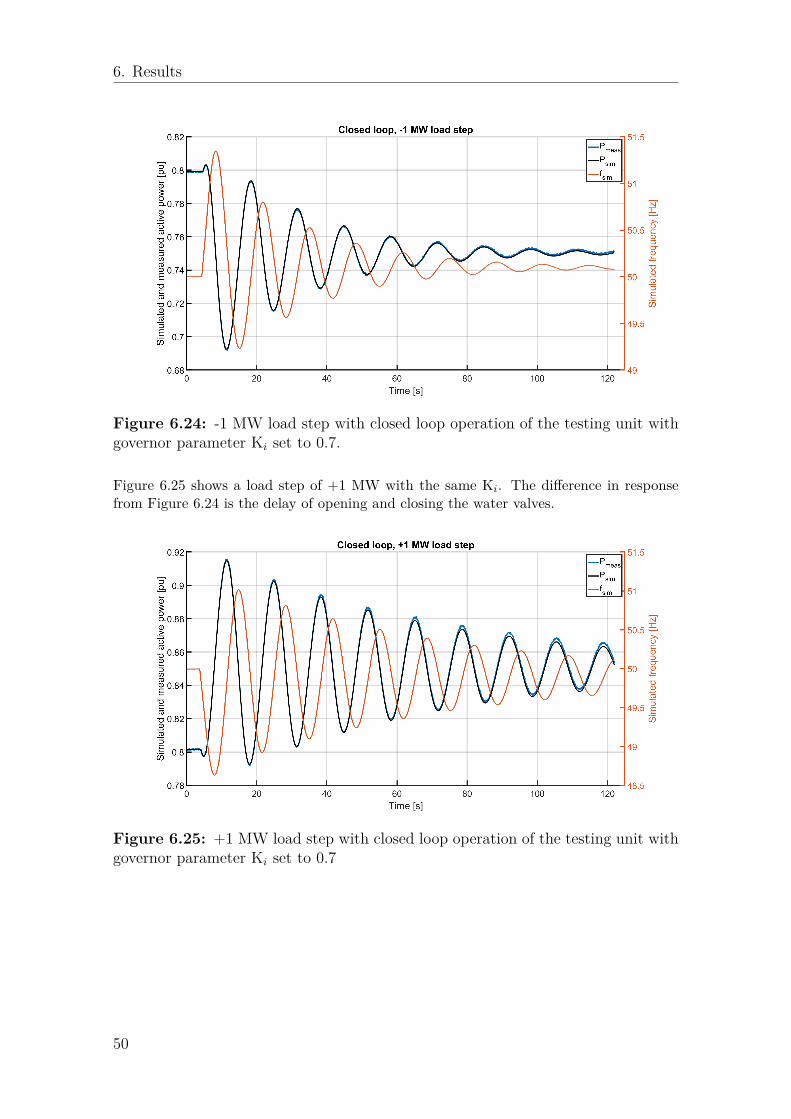
ones but as time continues it decreases to a value lower than the simulated. Figure 6.23shows a close up of the crossing.
Figure 6.22: +1 MW load step with closed loop operation of the testing unit.
Figure 6.23: +1 MW load step with closed loop operation of the testing unit.Simulated and measured active power crossing.
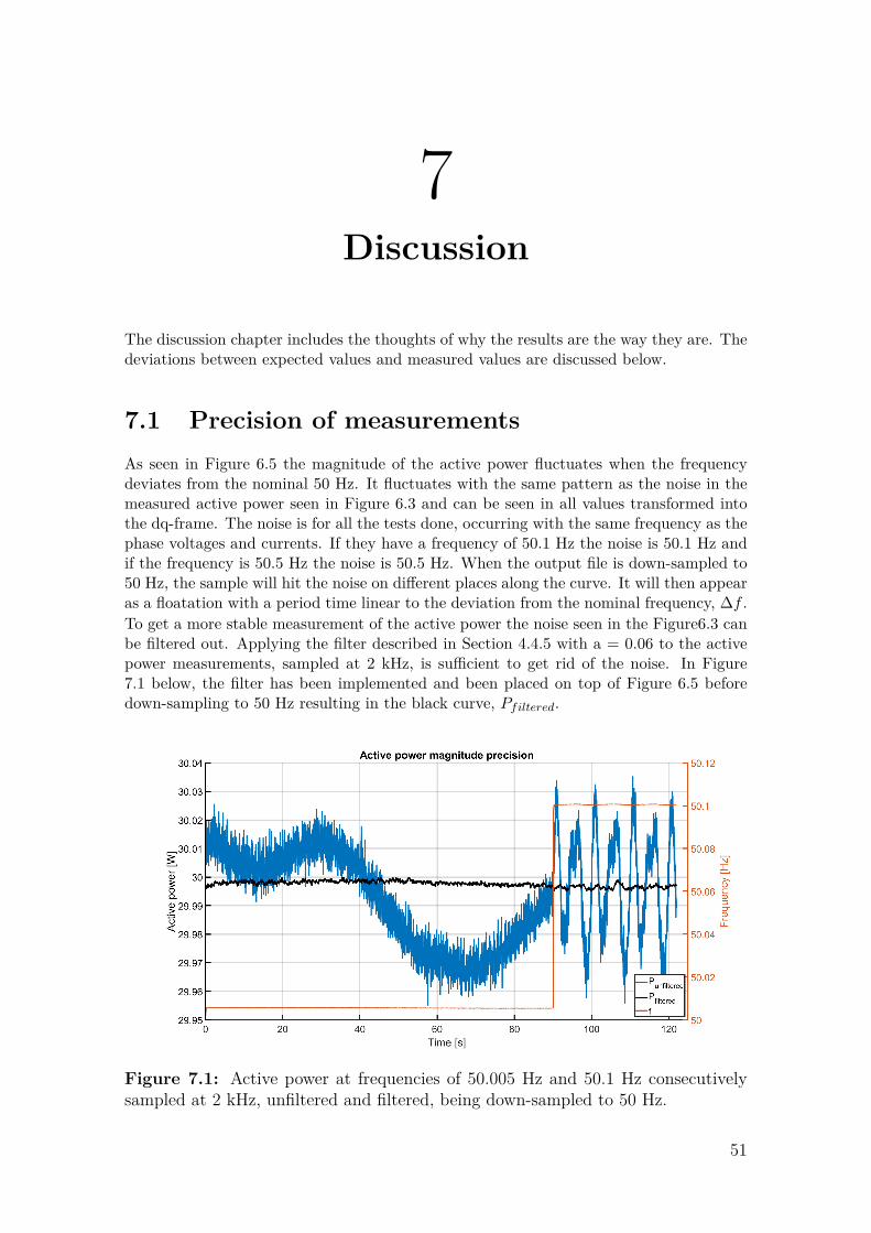
The value of Ki is changed to 0.7 and a step of -1 MW is applied seen in Figure 6.24. Theoutput response is with this parameterisation is more volatile then in Figure 6.21 and thesteady state is never reached during the simulation.
49
6. Results
Figure 6.24: -1 MW load step with closed loop operation of the testing unit withgovernor parameter Ki set to 0.7.
Figure 6.25 shows a load step of +1 MW with the same Ki. The difference in responsefrom Figure 6.24 is the delay of opening and closing the water valves.
Figure 6.25: +1 MW load step with closed loop operation of the testing unit withgovernor parameter Ki set to 0.7
50
7Discussion
The discussion chapter includes the thoughts of why the results are the way they are. Thedeviations between expected values and measured values are discussed below.
7.1 Precision of measurementsAs seen in Figure 6.5 the magnitude of the active power fluctuates when the frequencydeviates from the nominal 50 Hz. It fluctuates with the same pattern as the noise in themeasured active power seen in Figure 6.3 and can be seen in all values transformed intothe dq-frame. The noise is for all the tests done, occurring with the same frequency as thephase voltages and currents. If they have a frequency of 50.1 Hz the noise is 50.1 Hz andif the frequency is 50.5 Hz the noise is 50.5 Hz. When the output file is down-sampled to50 Hz, the sample will hit the noise on different places along the curve. It will then appearas a floatation with a period time linear to the deviation from the nominal frequency, ∆f .To get a more stable measurement of the active power the noise seen in the Figure6.3 canbe filtered out. Applying the filter described in Section 4.4.5 with a = 0.06 to the activepower measurements, sampled at 2 kHz, is sufficient to get rid of the noise. In Figure7.1 below, the filter has been implemented and been placed on top of Figure 6.5 beforedown-sampling to 50 Hz resulting in the black curve, Pfiltered.
Figure 7.1: Active power at frequencies of 50.005 Hz and 50.1 Hz consecutivelysampled at 2 kHz, unfiltered and filtered, being down-sampled to 50 Hz.
51
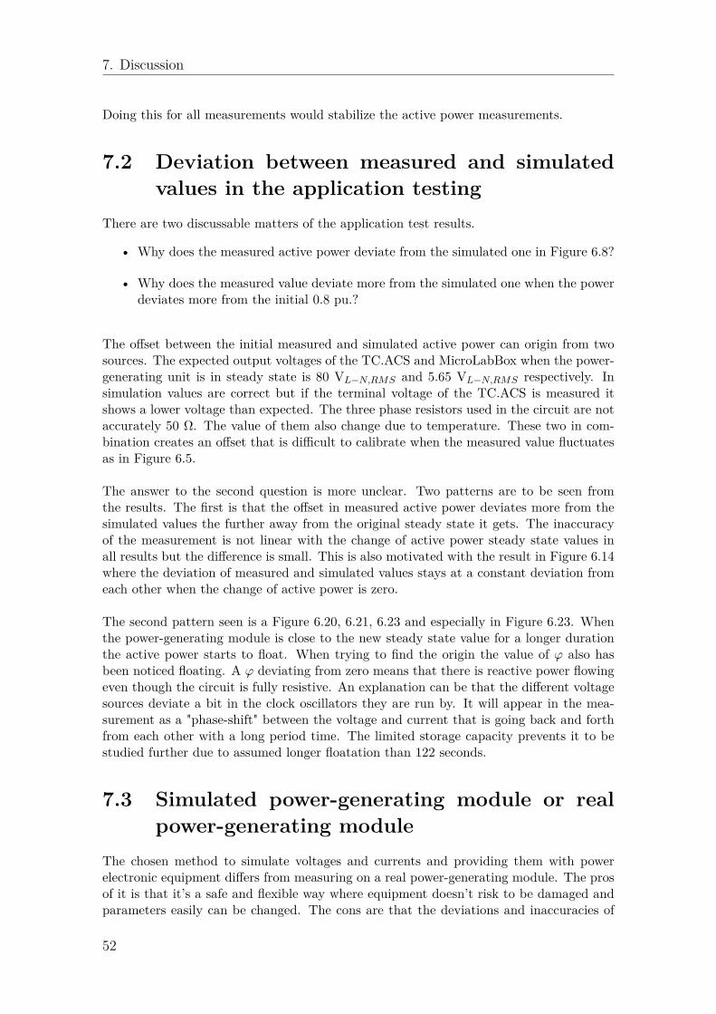
7. Discussion
Doing this for all measurements would stabilize the active power measurements.
7.2 Deviation between measured and simulatedvalues in the application testing
There are two discussable matters of the application test results.
• Why does the measured active power deviate from the simulated one in Figure 6.8?
• Why does the measured value deviate more from the simulated one when the powerdeviates more from the initial 0.8 pu.?
The offset between the initial measured and simulated active power can origin from twosources. The expected output voltages of the TC.ACS and MicroLabBox when the power-generating unit is in steady state is 80 VL−N,RMS and 5.65 VL−N,RMS respectively. Insimulation values are correct but if the terminal voltage of the TC.ACS is measured itshows a lower voltage than expected. The three phase resistors used in the circuit are notaccurately 50 Ω. The value of them also change due to temperature. These two in com-bination creates an offset that is difficult to calibrate when the measured value fluctuatesas in Figure 6.5.
The answer to the second question is more unclear. Two patterns are to be seen fromthe results. The first is that the offset in measured active power deviates more from thesimulated values the further away from the original steady state it gets. The inaccuracyof the measurement is not linear with the change of active power steady state values inall results but the difference is small. This is also motivated with the result in Figure 6.14where the deviation of measured and simulated values stays at a constant deviation fromeach other when the change of active power is zero.
The second pattern seen is a Figure 6.20, 6.21, 6.23 and especially in Figure 6.23. Whenthe power-generating module is close to the new steady state value for a longer durationthe active power starts to float. When trying to find the origin the value of ϕ also hasbeen noticed floating. A ϕ deviating from zero means that there is reactive power flowingeven though the circuit is fully resistive. An explanation can be that the different voltagesources deviate a bit in the clock oscillators they are run by. It will appear in the mea-surement as a "phase-shift" between the voltage and current that is going back and forthfrom each other with a long period time. The limited storage capacity prevents it to bestudied further due to assumed longer floatation than 122 seconds.
7.3 Simulated power-generating module or realpower-generating module
The chosen method to simulate voltages and currents and providing them with powerelectronic equipment differs from measuring on a real power-generating module. The prosof it is that it’s a safe and flexible way where equipment doesn’t risk to be damaged andparameters easily can be changed. The cons are that the deviations and inaccuracies of
52
7. Discussion
measurements are explained by other reasons.
The Simulink model has been a perfect tool to study a power-generating module’s depen-dency on different parameter values. The usage of testing the code under ideal conditionshas been a perfect way to get a hint if it’s going to work or not. It’s also been easy tocompile into ControlDesk.
The case of using different sources for provision of voltage and current may cause differentmagnitude deviations or phase positions from each other due to delays and noise of theequipment. Measuring with voltage and current transformers on a real power-generatingmodule has the benefit that the signals come from the same analog source.
7.4 Importance of parametrisation of the gover-nor
For frequency regulation, the results shows the importance of having a tuned parametri-sation of the governor. For open loop operation of the testing unit and the Ki value setto 0.7 the power-generating module would be approved for FCR-N but not for FCR-Daccording to the technical requirements in Section 2.3. For the closed loop operation thetechnical requirements are unknown but it’s clearly seen that a value of Ki set to 0.07 ismore stable and has a faster regulation compared to the ones with Ki set to 0.7.
7.5 Future studiesTo improve the testing unit it’s suggested to apply the filter described in 7.1 and tune itto it’s application to ensure a better accuracy.
To improve the application tests setup it’s suggested to find the reasons to the inac-curacies of the measured active power from the TC.ACS or the MicroLabBox.
The next step would be to test the unit on a real power-generating unit and study thedifferences.
53

7. Discussion
54
8Conclusion
In this chapter the results are compared to the technical requirements and to the aim.
The testing unit is able to meet the technical requirements for testing of FCR provi-sion in the Nordic synchronous area. The requirements states that the instantaneouspower measurements must have a minimum accuracy of 0.5 % of the rated power of theproviding entity, which the results from precision testing of the testing unit holds true.The frequency measurement requirements of 1 mHz resolution and 10 mHz accuracy isalso met by the testing unit, with a resolution of < 0.2 mHz and accuracy of < 1 mHz,from the precision tests.
The aim of the report, to develop a testing unit able to test the frequency controllingperformance of a power-generating module, is accomplished.
55

8. Conclusion
56
Bibliography
[1] N. Ung, “The effects of backlash on the frequency stability in a hydro basedpower system,” [Online]. Available: http://www.svk.se/siteassets/jobba-har/dokument/the- effects- backlash- on- frequency- stability- in-hydro-based-power-system.pdf.
[2] H. Engel, R. Hensley, S. Knupfer, and S. Sahdev, “The Potential Impactof Electric Vehicles on Global Energy Systems,” McKinsey Center for Fu-ture Mobility, no. Exhibit 1, p. 8, 2018. [Online]. Available: https://www.mckinsey.com/industries/automotive- and- assembly/our- insights/the- potential- impact- of- electric- vehicles- on- global- energy-systems.
[3] ENTSO-E, “Nordic Report: Future System Inertia,” Nordic Report, pp. 1–58,2017. [Online]. Available: https://www.entsoe.eu/Documents/Publications/SOC/Nordic/Nordic_report_Future_System_Inertia.pdf.
[4] E. Agneholm, N. Krantz, M. Emanuelsson, H. Hermansson, S. Ab, S. Kraft-nät, and V. A. Elproduktion, “Solvsim Power Station – a New Safe Way ofTesting the Frequency Control and Island Operation Capability of Power Sta-tions,” 2002. [Online]. Available: http://pscc.ee.ethz.ch/uploads/tx_ethpublications/s06p06.pdf.
[5] European Union, “Commission Regulation (Eu) 2016/631,” Official Journalof the European Union, no. 14 April 2016, p. 68, 2016.
[6] “Energimarknadsinspektionens författningssamling Energimarknadsinspektio-nens föreskrifter nätanslutning av generatorer ;,” 2018. [Online]. Available:https://www.ei.se/Documents/Publikationer/foreskrifter/El/EIFS_2018_2.pdf.
[7] Fingrid, “Frequency Quality Analysis 2019 FINGRID,” 2019. [Online]. Avail-able: https://www.fingrid.fi/en/grid/power-transmission/maintenance-of-power-balance/.
[8] M. Kuivaniemi, Frequency - historical data [CSV-file from Fingrid Oyj]. [On-line]. Available: https : / / data . fingrid . fi / en / dataset / frequency -historical-data.
[9] Svenska Kraftnät, “Årsredovisning 2019,” 2019. [Online]. Available: https://www.svk.se/press-och-nyheter/nyheter/allmanna-nyheter/2020/arsredovisning-2019/.
[10] ——, “Ödrift - För att säkerställa elförsörjning i krissituationer,” [Online].Available: https://www.svk.se/sakerhet-och-hallbarhet/elberedskap/.
[11] IEEE board, “IEEE Policies 2014,” no. February, 2014. [Online]. Available:https://www.ieee.org/about/corporate/governance/p7-8.html.
57
Bibliography
[12] P. Chen, PSAC SS5b FrequencyRestorationProcess [PowerPoint slides], 2020.[13] Svenska Kraftnät, “Villkor för FCR,” vol. 1, no. 16, pp. 1–16, [Online]. Avail-
able: https://www.svk.se/aktorsportalen/elmarknad/balansansvar/balansansvarsavtal/.
[14] P. W. Group, “Supporting Document on Technical Requirements for Fre-quency Containment Reserve Provision in the Nordic Synchronous Area Draft2017 Prequalification Working Group , FCP project THE REQUIREMENTSARE SO FAR DRAFT REQUIREMENTS,” no. June, 2017.
[15] “Turbine Governor Test Equipment,” no. July, pp. 1–30, 2019.[16] F. Fjärrterminal, “Feldetektor och Fjärrterminal,” 2005. [Online]. Available:
https://www.protrol.se/uploaded_files/IPC4020_datablad_2005_se1.pdf?v20200515104610.
[17] L. Harnefors, “Control of Variable-Speed Drives,” Applied signal processingand control department of electronics, Mälardalen university, 2002.
[18] M. Bongiorno, J. Svensson, and A. Sannino, “Effect of sampling frequency andharmonics on delay-based phase-sequence estimation method,” IEEE Trans-actions on Power Delivery, vol. 23, no. 3, pp. 1664–1672, 2008, issn: 08858977.doi: 10.1109/TPWRD.2008.915802.
[19] P. Kundur, Power System Stability And Control, 1994.
58

![[Compliance Presentation Title/Subject] · function. Compliance Testing is the independent testing arm of the Citi Compliance function. Our mission is to: Compliance Testing plans](https://static.fdocuments.us/doc/165x107/5e47b61e9e5ff6667e3cd0eb/compliance-presentation-titlesubject-function-compliance-testing-is-the-independent.jpg)