Geophys. J. Int. (2019) 218, 787–800 doi: 10.1093/gji/ggz191Advance Access publication 2019 April 26GJI Seismology

Testing the limits of virtual deep seismic sounding via new crustalthickness estimates of the Australian continent

D. A. Thompson ,1,2 N. Rawlinson2,3 and H. Tkalcic4

1School of Earth and Ocean Sciences, Cardiff University, Cardiff, UK. E-mail: thompsond10@cardiff.ac.uk2Department of Geology and Petroleum Geology, University of Aberdeen, Aberdeen, UK3Department of Earth Sciences-Bullard Laboratories, University of Cambridge, Cambridge, UK4Research School of Earth Sciences, Australian National University, Canberra, Australia

Accepted 2019 April 25. Received 2019 March 2; in original form 2018 September 7

S U M M A R YWe apply virtual deep seismic sounding (VDSS) to data collected from both permanent andtemporary seismic stations in Australia with the goal of examining (i) the resilience of themethod to the presence of complex lithospheric structure and (ii) the effectiveness of differentapproaches for estimating bulk crustal properties (namely thickness and Vp). Data from thepermanent station WRAB in the Northern Territory is ideal for benchmarking VDSS (largenumber and favourable distribution of recorded earthquakes), with the results from severalapproaches agreeing on a thickness of 40–42 km. Application of VDSS to data from thetemporary BILBY array, a linear distribution of broadband stations that traverses centralAustralia, shows that strong Moho reflections can be retrieved with as few as two earthquakeseven at the transition between crustal blocks of different character and in the presence ofthick sedimentary basins. Crustal thickness varies between 36 and 54 km and compares wellwith the reflectivity character of nearby deep seismic reflection lines. Furthermore, we findthat off-line estimates of crustal thickness, calculated by binning the source regions accordingto back-azimuth, produce values of crustal thickness that are consistent with the regionalgeology. Overall, we find that VDSS is a powerful technique for estimating crustal thicknessand velocity due to its insensitivity to complex short-wavelength structure and requirement ofa small number earthquakes to produce a stable result. However, not all schemes tested forextracting bulk crustal properties appear to be robust and stringent data quality checking isstill required during implementation.

Key words: Composition and structure of the continental crust; Australia; Body waves;Crustal imaging; Crustal structure.

1 I N T RO D U C T I O N

Australia has a long and convoluted tectonic history that has ledto a complicated present day lithospheric structure. Major oro-genic episodes have resulted in continental growth and rework-ing of older material (e.g. Musgrave, Arunta, Petermann and Al-ice Springs Orogens; Betts et al. 2002; Cawood & Korsch 2008)while major sedimentary basins have formed in response to ex-tensional tectonics (e.g. Amadeus, Officer and Georgina Basins;Walter et al. 1995). These structures can be problematic for typi-cal high-frequency passive seismic imaging tools such as P-wavereceiver functions because of energy becoming trapped within thelow-velocity sediments or because of complex signatures preservedat the crust–mantle boundary (Clitheroe et al. 2000; e.g. Langston2011). It is therefore desirable to implement a technique that is rel-atively insensitive to these complications, but that can still provide

important first-order information on crustal structure (i.e. crustalthickness, bulk velocity).

The virtual deep seismic sounding (VDSS) method is a rela-tively new approach that utilizes incident S-waves from earthquake-receiver distances of 30◦–50◦ (Tseng et al. 2009; Yu et al. 2012,2013). A free surface conversion from S to P leads to a top-side Moho reflection, analogous to conventional active sourcedeep seismic sounding, that has an extremely high signal-to-noise ratio and is low enough frequency to be insensitive tocomplicated small-scale structure. It has been used to delineatecrustal thickness variations in regions that are expected to havecomplex Moho signatures (e.g. Tibet and Ordos Plateau; Tsenget al. 2009; Yu et al. 2012), significant sedimentary cover (East-ern USA; Parker et al. 2016) and where large crustal variationslikely cause differences in isostatic compensation (Western USA;Yu et al. 2016).

C© The Author(s) 2019. Published by Oxford University Press on behalf of The Royal Astronomical Society. 787

Dow

nloaded from https://academ

ic.oup.com/gji/article-abstract/218/2/787/5480468 by Library user on 20 August 2019

788 D. A. Thompson, N. Rawlinson and H. Tkalcic

In this paper, we implement the VDSS method on two geographi-cally co-located datasets of contrasting deployment times and applya variety of migration and waveform modelling techniques to test thelimits of its applicability. Australia is the ideal natural laboratory fortesting VDSS given that it has complex lithospheric structures thatthe method is hypothesized to be insensitive to and is surroundedby seismogenic zones in the desired distance range. The approachcan provide robust results using comparatively few traces due to thesignal-to-noise ratio achieved. Despite this, we also highlight thatcertain modelling approaches can return spurious results even forvoluminous high quality data set.

2 G E O L O G I C A L S E T T I N G A N DP R E V I O U S G E O P H Y S I C A L S T U D I E S

The geology of Central Australia is dominated both by orogenyand widespread sedimentary sequences that range in age from Pa-leoproterozoic to Carboniferous (e.g. Cawood & Korsch 2008).The oldest terrane to be imaged by this study is the Arunta Block(Fig. 1), sometimes referred to as the Arunta Orogen. It comprisesPaleoproterozoic (1880-1800 Ma) sequences with various stages oftectonic activity being recorded as late as ∼1580 Ma (Cawood &Korsch 2008). The 1.30–1.10 Ga collision of the South AustralianCraton (containing the Gawler Craton, see Fig. 1) with the previ-ously amalgamated North and West Australian Cratons is preservedin the Musgrave Block (Betts et al. 2002; Howard et al. 2015),bounded in the north by the Amadeus Basin and to the south bythe Officer Basin (Fig. 1). Subsequent 1.10-1.00 Ga dyke emplace-ment and volcanism was followed by a period of quiescence thatculminated in uplift and further magmatism at ∼800 Ma. The ori-gin of this volcanism is believed to be due to the impingementof a mantle plume (Zhao et al. 1994) with subsequent extensionand crustal sagging forming the Centralian Superbasin (encompass-ing the vast majority of what is now Central Australia, includingthe Musgrave Block, Amadeus Basin, Officer Basin and southernGeorgina Basin; Walter et al. 1995). The current geometry of sed-imentary basins was achieved by segmentation of the CentralianSuperbasin due to two major phases of intraplate deformation asso-ciated with Neoproterozoic–Cambrian and Carboniferous orogeny.The Petermann Orogen (580–540 Ma) was focussed at the margin ofthe Amadeus Basin and Musgrave Block (Fig. 1). The Alice SpringsOrogen (∼320 Ma) reactivated structures along the northern marginof the Amadeus Basin, most notably the Redbank Shear Zone. Thisfocussed reactivation has led to large Moho offsets being preservedacross major faults by as much as 20 km in places (e.g. Goleby et al.1989).

On the broadest scale, surface wave analysis has mapped the longwavelength features of the Australian continent to asthenosphericdepths highlighting a strong east–west change between the ancient(Proterozoic and older, >1.1 Ga) domains of central/western Aus-tralia and the younger (<1 Ga) regions of eastern Australia (Fish-wick et al. 2005). The older terranes to the west of ∼140◦E (broadlycorresponding with a feature referred to as the Tasman Line) ex-hibit fast seismic velocities to depths of 200 km or greater whichis indicative of a thick, cold cratonic root often observed beneathsurface geology of this age (Polet & Anderson 1995; Kennett et al.2004; Fishwick et al. 2005; ). Despite this finding, the shallowestparts of the surface wave model (∼75 km depth) exhibit lower thanexpected seismic velocities which are also confirmed by body-waveobservations (Kaiho & Kennett 2000; Fishwick et al. 2008). Recent

Pn tomography work has identified a more complex pattern of litho-spheric velocity variations within our study area in central Australiaand conclude that regions exhibiting low mantle P-wave velocities(<8.0 km s−1) are likely affected by velocity gradients in regions ofthickened crust (Sun & Kennett 2016). Ambient noise tomographyhas also shown a complex pattern of crustal structure throughoutCentral Australia, including the signatures of the aforementionedsedimentary basins and Proterozoic collisional zones (Saygin &Kennett 2012). This type of study benefits from utilising higherfrequency surface waves for determination of shallower structure(<40 km), but for regions of thicker crust this sensitivity remainspoor (Saygin & Kennett 2012). P-to-S energy converted at the Mohovia the receiver function method again shows the presence of largevariations in crustal thickness that correlate with the major tectonicblocks of central Australia, with thicker crust (>50 km) and a dif-fusive Moho signature at the northern and southern margins of theAmadeus Basin (Sippl 2016). The diffusive nature of the Moho hasmade it difficult to derive a definitive crustal thickness at several ofthese localities (Sippl 2016). Active source seismic surveys providethe highest frequency probe of deep crustal structure, but are gen-erally limited to 2-D transects which provide limited geographicalcoverage. Sharp changes in crustal thickness, in excess of 25 km ofvertical Moho displacement across the Redbank Shear Zone at thenorthern margin of the Amadeus Basin (Fig. 1), were identified inearly crustal-scale reflection profiles (Goleby et al. 1989; Korschet al. 1998). A large number of seismic reflection transects have beenperformed across the Australian continent since these early studies(comprehensively reviewed by Kennett & Saygin 2015), with majorfindings including that the central Australian crust exhibits distinctjumps (8–10 km in places in addition to the previously mentionedvariations) in Moho geometry along with regions where the reflec-tivity character makes definitive determination of crustal thicknessimpossible (Kennett & Saygin 2015; Kennett et al. 2016; Korsch &Doublier 2016).

Based on the complexity of the surface geology/lithosphericstructures observed, the availability of broadband seismic datatraversing these terranes, co-located active source seismic stud-ies and the unavoidable technical difficulties faced by the commonsuite of geophysical techniques implemented in the region, it is clearthat central Australia represents the ideal region in which to test thelimits and sensitivities of the VDSS methodology.

3 DATA A N D M E T H O D S

3.1 Seismic stations

Permanent station WRAB (Streckeisen STS-2 shallow surface vaultseismometer; part of the IRIS-IDA Global Seismograph Network)is located at the Warramunga Seismic Array in northern Australia(Fig. 1) and has been recording continuously since 1994. We also in-corporate data from the temporary BILBY seismic network (Rawl-inson & Kennett 2008), a 23 station linear broadband network thatwas operational between 2008 and 2011 (Fig. 1, see Sippl 2016,for details).

Earthquakes of M5.5+ for the distance range of 20◦–60◦ wereselected for pre-processing, with a visual inspection of traces beingperformed to remove events that were poorly recorded. Data wereinitially filtered with a 2nd order zero phase Butterworth bandpassfilter with corner frequencies of 0.05 and 0.5 Hz with the hori-zontal components being subsequently rotated into the radial andtangential components for further processing.

Dow

nloaded from https://academ

ic.oup.com/gji/article-abstract/218/2/787/5480468 by Library user on 20 August 2019

Limits of virtual deep seismic sounding 789

130˚

130˚

135˚

135˚

140˚

140˚

35˚ 35˚

30˚ 30˚

25˚ 25˚

20˚ 20˚

15˚ 15˚

130˚

130˚

135˚

135˚

140˚

140˚

35˚

30˚

25˚

20˚

15˚

BL07BL08BL09BL10BL11BL12BL13BL14BL15BL16BL17BL18BL19BL20

WRABBL01

BL02

BL05BL06

Officer

Musgrave

Amadeus

Arunta

NB

Gawler

Georgina

10°20°30°40°50°60°

Figure 1. (a) Map of the Australian continent showing the locations of broadband seismometers used in this study and the main geological terranes. NB,Ngalia Basin. Inset is the location of seismicity that contribute to the VDSS data set both for WRAB and the BILBY seismic network. Blue dots are eventswith shallow hypocentres (<410 km) and red are events with deep (>410 km) hypocentres.

Dow

nloaded from https://academ

ic.oup.com/gji/article-abstract/218/2/787/5480468 by Library user on 20 August 2019

790 D. A. Thompson, N. Rawlinson and H. Tkalcic

(a)

(b) (c)

Figure 2. (a) Results of the 1-D depth migration for WRAB. Black line is the whole data set, blue line is data from the easterly back-azimuthal corridor and redis data from the northerly back-azimuthal corridor. (b) VDSS traces binned by slowness. Clear moveout of the SsPmp phase is observed across the epicentraldistance range of interest (30◦–50◦), along with the presence of both the precursory Smp phase and the reverberatory SsPmsPmp phase. The dashed lines arethe predicted arrival times for the crustal thickness derived from the migration approach (full data set). (c) Same as (b), but with the best-fitting model from thesingle parameter (H) waveform inversion approach underlain. Amplitudes are scaled such that the direct S-waves in both the real data and the synthetic tracesare equal. Inset is a ray diagram of the main SsPmp waveform utilized during VDSS analysis (i = incidence angle at the Moho, and ic = critical angle).

3.2 Virtual deep seismic sounding

The VDSS method relies on the fact that the topside P-to-P reflec-tion from the Moho (following the preceding S-to-P conversion atthe free surface, Fig. 2) is post-critical and hence undergoes totalinternal reflection (Tseng et al. 2009). This provides the high signal-to-noise that characterizes VDSS observations, but also results in aphase shift of the SsPmp phase that needs to be taken into account.

The source normalization approach described by Yu et al. (2013)was implemented on the Australian data to remove source-side scat-tering effects, making events suitable for VDSS analysis regardlessof focal depth. We use the theoretical ray parameter (pβ ) and inci-dence angle (j) for the direct S-wave assuming the ak135 velocitymodel (Kennett et al. 1995; Crotwell et al. 1999) to calculate the

rotation required to transform the vertical and radial componentsinto the pseudo-S component (φ1) using the following equation:

tan(φ1) = (ηα/ηβ ) tan 2 j, (1)

where ηα and ηβ are the P-wave and S-wave vertical slownesses,(V ′−2

p − p2β )1/2 and (V ′−2

s − p2β )1/2, respectively, with V ′

P and V ′S

being the near surface P and S velocities (for further details, see Yuet al. 2013). Rotating into the pseudo-S component provides an esti-mate of the shear-wave source wavelet for the VDSS analysis, withthis being deconvolved from the vertical component seismogramusing an extended time multitaper approach (10 s sliding windowlength, 75 % window overlap, 3 Slepian tapers; Helffrich 2006). ForWRAB, this led to 294 VDSS traces across the 22-year deploymenthistory. The temporary nature of the BILBY deployment led to a

Dow

nloaded from https://academ

ic.oup.com/gji/article-abstract/218/2/787/5480468 by Library user on 20 August 2019

Limits of virtual deep seismic sounding 791

38

40

42

44

46

H e

stim

ate

(km

)

0 50 100 150 200 250 300

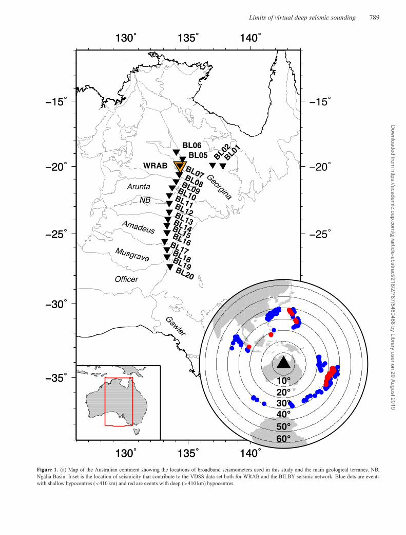
No. tracesFigure 3. Migration-based results from station WRAB for a range of data subsets (traces varying from 5 to the whole data set of 294). All subsets bar the60-trace subset lie within error of the whole data set result of 41.2 ± 0.5 km (dashed line).

35

40

45

50

H(k

m)

14.0 14.5 15.0 15.5

Slowness(s/deg)Figure 4. Comparison between the results of the VDSS trace migration approach using synthetic data for a 42-km-thick crust with a uniform Vp of 6.5 km s−1

(filled circles) and WRAB data sorted into 0.2 s deg−1 bins with 50 % overlap between bins (triangles). The dashed line is the true crustal thickness of thesynthetic model (42 km).

Dow

nloaded from https://academ

ic.oup.com/gji/article-abstract/218/2/787/5480468 by Library user on 20 August 2019

792 D. A. Thompson, N. Rawlinson and H. Tkalcic

Figure 5. Results of the simultaneous H–Vp inversion for WRAB. (a) Histogram of crustal thickness showing the best-fitting 50 (red), 100 (blue) and 150(black) models. (b) Histogram of crustal Vp (colour convention follows a). (c) Stacked VDSS traces with slowness. The synthetic traces for the best-fitting 50models are plotted in red.

significantly reduced number of usable traces, varying between 2and 19 traces per station. For each station, VDSS traces were binnedand stacked by slowness in 0.2 s deg−1 bins with 50 % overlap (seeFig. 2 for WRAB and supporting information for BILBY stations).A minimum of 3 traces were required to produce a stacked trace.

The data set was then interrogated using a variety of approacheswith the goal of assessing their robustness and repeatability bothfor a voluminous, high-quality data set (WRAB) and a compara-tively data-poor but geographically co-located seismic deployment(BILBY).

Firstly, a new migration-based approach was developed to mapthe seismic energy to depth assuming a single layer crust. Theworkflow is built upon receiver function migration (Wilson & Aster2003; Angus et al. 2009; Hammond et al. 2011; Thompson et al.2011, 2015) edited to incorporate the different geometry of theSsPmp phase. Given that the arrival time of this phase relative tothe incident S-wave in a constant velocity medium is:

TSs Pmp−Ss = 2H (V −2p − p2

β )1/2, (2)

where pβ is determined using the known source-receiver geometryand the ak135 velocity model (Crotwell et al. 1999), it is possible toconvert the arrival time into a depth by assuming a crustal velocity.We present results for an assumed P-wave velocity of 6.5 km s−1 andVp/Vs ratio of 1.73, but also provide results with Vp of 6.4 km s−1

and 6.6 km s−1 in the supporting information. Due to its post-criticalnature, the SsPmp arrival undergoes a phase shift of ∼π /2, leadingto the arrival time being manifested as a zero crossing as opposed toan amplitude maximum typical of other methodologies. Therefore,we migrate all traces at a given station to depth using the aforemen-tioned approach, producing a summary depth trace through linear

stacking and derive crustal thickness by determining the depth atwhich the zero-crossing occurs. Error estimates on this value areobtained by bootstrapping the input data 100 times (Efron & Tib-shirani 1991), randomly selecting traces from the data set up to theoriginal number (allowing repetition). We also attempt to removethe effect of the phase shift by calculating the envelope function(Bracewell 1978; Phinney et al. 1981; Parker et al. 2016) for allavailable VDSS traces and migrating these to depth using the sameapproach described above. Using the envelope functions, the arrivaltime would be seen as a positive peak in the stacked migrated trace.

Previous studies have relied on waveform modelling to determinecrustal thickness, and where a range of slownesses were available,to determine crustal Vp (Tseng et al. 2009; Yu et al. 2016). Weuse a similar approach to initially invert for H alone. Each of theslowness bins were used as input traces to model synthetic waveformdata for a simple layer over a half space, allowing crustal thicknessto vary between 30 and 55 km in 0.2 km increments. Synthetictraces were produced using the reflectivity method (Fuchs & Muller1971; Kennett 1983). Each model was compared to the real data bycalculating the L2 norm, with quoted values being the model withminimum misfit and associated errors calculated by repeating theprocess with Vp of 6.4 km s−1 and 6.6 km s−1.

It is not just the SsPmp phase that is present in the recorded traces,with the precursory Smp and reverberatory SsPmsPmp phases alsoappearing as strong arrivals (see Fig. 2 and supporting information).The time window over which the misfit was calculated is hence −10to +30 s relative to the direct S-wave arrival in order to incorporatethese observed phases. The same approach was used to simultane-ously invert for H and Vp (herein referred to as the simultaneousH–Vp inversion) with the same range of H but allowing Vp to vary

Dow

nloaded from https://academ

ic.oup.com/gji/article-abstract/218/2/787/5480468 by Library user on 20 August 2019

Limits of virtual deep seismic sounding 793

14.0

14.2

14.4

14.6

14.8

15.0

15.2

15.4

15.6

Slo

wne

ss(s

/deg

)

−5 0 5 10 15

Time(s)

WRAB

14.0

14.2

14.4

14.6

14.8

15.0

15.2

15.4

15.6

Slo

wne

ss(s

/deg

)

−5 0 5 10 15

Time(s)Figure 6. Envelope functions for station WRAB. Red dots are the max-imum amplitude picks for the SsPmp phase and the dashed curve is thepredicted moveout curve for the result of the migration based approach withan assumed crustal Vp of 6.5 s km−1.

between 6.1 km s−1 and 6.9 km s−1 in increments of 0.02 km s−1.In this case, quoted values are the average H and Vp from the 150best-fitting models.

Unlike SsPmp, the arrival times of Smp and SsPmsPmp are de-pendent on the Vp/Vs ratio. In addition to this, the relative timing ofmany of the phases of interest (Smp, SsPmsPmp) and the distance atwhich SsPmp becomes post-critical is also dependent on the crustalVp/Vs ratio and uppermost mantle velocity. To investigate the sensi-tivity of the data set to these parameters, we also attempted to invertfor H, Vp, Vp/Vs ratio and Pn velocity simultaneously.

The final method was the linear regression approach of Kanget al. (2016), where fitting a straight line through the SsPmp trav-eltime picks plotted in the form of p2

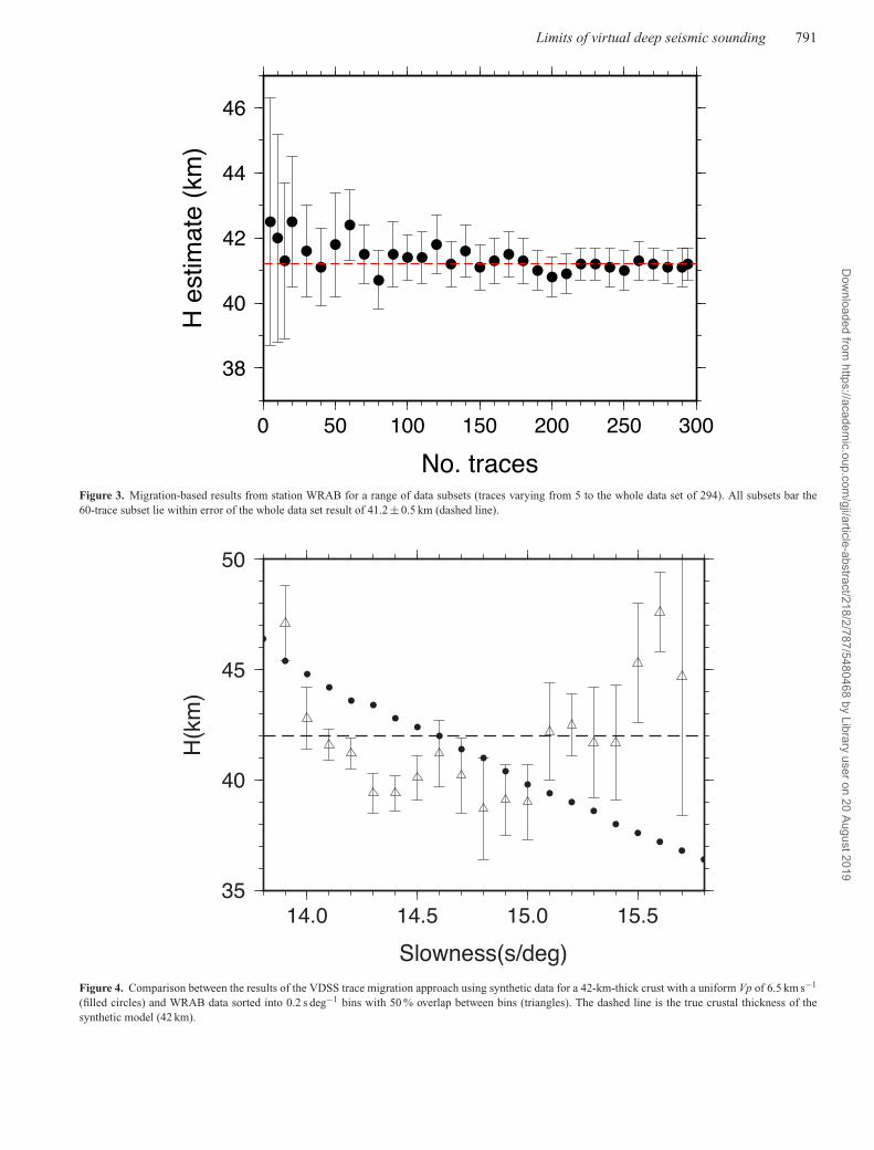
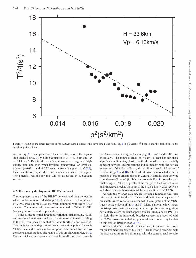
β versus T2/4 allows for thedetermination of H and Vp. Traveltimes were derived from the en-velope functions of each slowness bin to negate the phase shift ofthe post-critical reflection.

4 R E S U LT S

4.1 Permanent station: WRAB

The large data set (294 VDSS traces) and excellent slowness cov-erage (13.9–15.7 s deg−1) that WRAB provides is an ideal data setwith which to benchmark the VDSS method (Figs 2a–c). The main

phase of interest, the post-critical SsPmp reflection, is clearly ob-served with high signal-to-noise across the whole slowness rangewith an arrival time (relative to the phase Ss) varying from ∼6 s to8 s (Figs 2b and c). The precursory Smp phase can be seen arriving∼6 s prior to the direct S-wave in most bins, and the reverberatorySsPmsPmp is also clearly observed at times of 16–22 s (Figs 2b andc).

The migration-based approach returned a crustal thickness of41.2 ± 0.5 km (mean and 2σ data uncertainty); the summary mi-grated trace can be seen in Fig. 2(a). In order to utilize the largedata set and test the stability of this result, a number of data subsetswere randomly created (without allowing repetition of traces) forsample sizes ranging from five traces to the maximum 294. Theresults of this process can be seen in Fig. 3. All data subsets (withthe exception of the group containing 60 traces) lie within error ofthe result from the entire WRAB data set, highlighting the robust-ness of the H estimates even with a comparatively small number oftraces. Errors gradually reduce from ±3.8 km for 5 traces to ±1 kmor less for subsets of >70 traces (Fig. 3).

Despite being able to provide a single migration result for agiven station, we also investigate back-azimuthal variations by bin-ning data from the two dominant source regions (notably the Javasubduction system to the north and the Tonga-Fiji subduction sys-tem to the east). Fig. 2 shows that the migrated traces for both ofthese source regions are extremely similar with the results beingwithin error of each other (40.8 ± 0.6 km for the easterly data setand 41.6 ± 0.9 km for the northerly data set).

Due to the assumption of the migration approach that the zerocrossing represents the arrival time of the SsPmp phase, there maybe inherent bias in the crustal thickness estimate due to the fact thatthe phase shift is not equal to π /2 at all slownesses. This has beeninvestigated both through tests on synthetic data for a 42-km-thickcrust (Vp = 6.5 km s−1, based on the migration based result of 41.2± 0.5 km) and by binning the WRAB data set into 0.2 s deg−1 binswith 50 % overlap (Fig. 4). The maximum deviation due to thezero crossing assumption in the synthetic data set (filled circlesin Fig. 4) is ∼5 km below the true thickness at the high slownessend of the data coverage (15.7 s deg−1). The real data from WRABdoes not follow the expected pattern identified in the synthetic data,with most bins below 14.6 s deg−1 exhibiting lower values than thesynthetic values and the majority of bins above 15.0 s deg−1 showinggreater values than expected based on the synthetic tests.

The envelope function migration returned a value of 39.6 ±0.8 km, close to the result of the VDSS trace result of 41.2 ±0.5 km. The close agreement of these two approaches is likely dueto the excellent slowness coverage of the WRAB data set averagingout any potential bias due to the zero crossing assumption inherentto the VDSS trace migration approach.

The single parameter inversion gave a similar crustal thickness of42.4 ± 2.4 km (Table S1) and the simultaneous H–Vp inversion gaveestimates of H = 39.6 ± 3.3 km and Vp = 6.36 ± 0.16 km s−1 (Fig. 5and Table S3), also within error of both migration approaches. Re-sults from the simultaneous H–Vp inversion obtained by minimizingthe L1 norm give similar results (H = 40.7 ± 3.3 km and Vp = 6.40± 0.16 km s−1). The four parameter inversion shows H an Vp es-timates consistent with the previously discussed approaches (40.1± 5 km and 6.36 ± 0.2 km s−1) but only a weak dependance onVp/Vs (1.73 ± 0.07) and Pn velocity (8.3 ± 0.3 km s−1) based onthe broad spread in the histogram (Fig. S1 and Table S3).

The envelope functions, including the SsPmp−Ss traveltime pickderived from the traces themselves and the predicted traveltimecurve based on the result from the migration approach, can be

Dow

nloaded from https://academ

ic.oup.com/gji/article-abstract/218/2/787/5480468 by Library user on 20 August 2019

794 D. A. Thompson, N. Rawlinson and H. Tkalcic

6

8

10

12

14

16

18T

2 /4(

s2 )

0.014 0.016 0.018 0.020

p2(s2/km2)

H = 33.6km

Vp = 6.13km/s

Figure 7. Result of the linear regression for WRAB. Data points are the traveltime picks from Fig. 6 in p2β versus T2/4 space and the dashed line is the

best-fitting straight line.

seen in Fig. 6. These picks were then used to perform the regres-sion analysis (Fig. 7), yielding estimates of H = 33.6 km and Vp= 6.1 km s−1. Despite the excellent slowness coverage and highquality data, and even when invoking conservative 2σ error es-timates (±6.6 km and ±0.32 km s−1) from Kang et al. (2016),these results were quite different to other studies of the region.The potential reasons for this will be discussed in subsequentsections.

4.2 Temporary deployment: BILBY network

The temporary nature of the BILBY network and long periods inwhich no data were recorded (Sippl 2016) has lead to a low numberof VDSS traces at most stations when compared with the WRABdata set. The number of traces are summarized in Tables S1–S12(varying between 2 and 19 per station).

To investigate potential directional variations in the results, VDSSand envelope function traces for each station were binned accordingto the two main back-azimuthal corridors (northerly and easterly).This included calcuting SsPmp Moho reflection points for eachVDSS trace and a mean reflection point determined for the twocorridors at each station. The results of this are shown in Figs. 8-10.Crustal thicknesses appear consistent from all directions beneath

the Amadeus and Georgina Basins (Fig. 8, ∼24◦S and ∼20◦S, re-spectively). The thinnest crust (35–40 km) is seen beneath thesesignificant sedimentary basins while the northern data, spatiallycoherent between several stations and coincident with the surfaceexpression of the Ngalia Basin, also exhibits crustal thicknesses of∼35 km (Figs 8 and 10). The thickest crust is associated with themargins of major crustal blocks in Central Australia. Data arrivingfrom the east (Tonga-Fiji subduction zone) in Fig. 8 shows the crustthickening to ∼50 km or greater at the margin of the Gawler Cratonand Musgrave Block to the south of the BILBY line (∼27.5–26.5◦S),and also at the southern extent of the Arunta Block (∼23.0◦S).

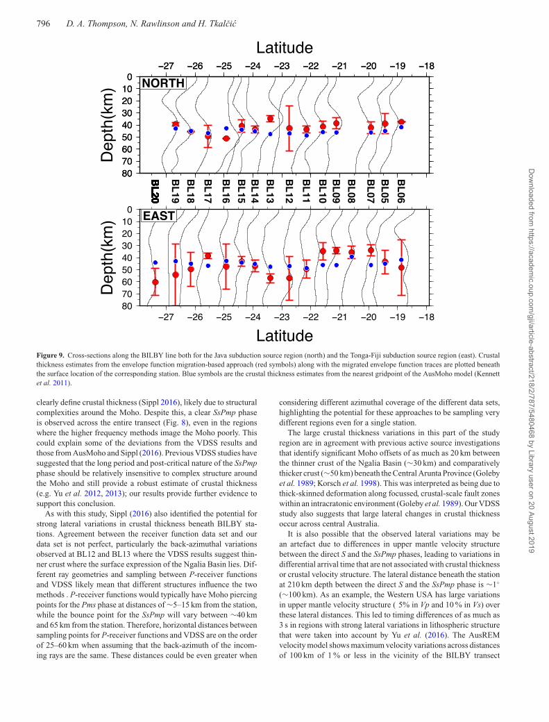
As with the WRAB data set, the envelope functions were alsomigrated to depth for the BILBY network, with the same pattern ofcrustal thickness variations as seen with the migration of the VDSStraces being evident (Figs 8 and 9). Many stations exhibit largerbootstrap error estimates using the envelope function migration,particularly where the crust appears thicker (BL12 and BL19). Thisis likely due to the inherently broader waveforms associated withthe SsPmp arrival time that are produced when converting the datain this fashion (Parker et al. 2016).

Where available, the single parameter waveform inversion resultsfor an assumed velocity of 6.5 km s−1 are in good agreement withthe associated migration estimates with the same crustal velocity

Dow

nloaded from https://academ

ic.oup.com/gji/article-abstract/218/2/787/5480468 by Library user on 20 August 2019

Limits of virtual deep seismic sounding 795

Figure 8. Cross-sections along the BILBY line both for the Java subduction source region (north) and the Tonga-Fiji subduction source region (east). Crustalthickness estimates from the VDSS trace migration-based approach (red symbols) along with the migrated VDSS traces are plotted beneath the surface locationof the corresponding station. Blue symbols are the crustal thickness estimates from the nearest gridpoint of the AusMoho model (Kennett et al. 2011).

(typically within error, see Fig. 11a and Tables S1–S12). This isreassuring given the identical crustal velocity assumed for the twoapproaches.

The general trend of thin crust within the Amadeus Basin andthicker crust at its margins is also seen in the simultaneous H–Vp in-version results (Table S2, Figs S26–S34). However, several stations(e.g. BL12, BL13 and BL14) have Vp values that are extremely vari-able, for example 6.21 km s−1 and 6.81 km s−1 at adjacent stations(Figs S28 and S29, respectively) and BL12 even showing a bimodaldistribution in its histograms (Fig. S27). This is highly likely to bedue to the large back-azimuthal variations observed and it is alsothese stations that tend to exhibit the poorest fits in the presentedslowness sections (Figs S11–S13). Several stations again agree towithin error when compared to the migration results (Fig. 11b), butthere are larger deviations evident than is observed when comparingthe results of the single parameter inversion (with the simultaneousH–Vp inversion crustal thickness estimates exhibiting significantlythinner crust than the migration results).

5 D I S C U S S I O N

The general pattern of crustal thickness is consistent with recentP-receiver function results from the BILBY array (Sippl 2016).

The thinnest crust is observed beneath the Amadeus and GeorginaBasins, with the thickest crust being observed at the northern mar-gin of the Amadeus Basin and the southern margin of the MusgraveBlock (Figs 8-10). An important observation is that high frequencyreceiver functions are complex in nature for the regions of thickercrust, making it difficult to obtain a confident estimate of crustalthickness (Sippl 2016). In contrast, the VDSS method retrieves aclear SsPmp phase from the Moho at all working stations includingthose expected to have complex Moho signatures (Fig. 8 and sup-porting information). This corroborates conclusions from previousVDSS studies in other localities (Tseng et al. 2009; Yu et al. 2012;Chen et al. 2013).

The AusMoho model of Kennett et al. (2011) incorporates arange of seismic data to produce crustal thickness estimates acrossthe Australian continent. The VDSS results are compared with Aus-Moho in Figs 8, 9 and 12. Most of the stations exhibit crustalthickness estimates that lie within error of the AusMoho predic-tion, although there are stations that deviate by significant amounts(10 km or more in places, BL20 and BL19 for example). Theseare mainly where the crust is expected to be at its thickest at themargin of the Gawler Craton and the Musgrave Block, and withinthe Arunta Block between the Amadeus and Georgina Basins (Ko-rsch & Doublier 2016). These are also regions where P-receiverfunctions have a diffuse Moho signature that make it problematic to

Dow

nloaded from https://academ

ic.oup.com/gji/article-abstract/218/2/787/5480468 by Library user on 20 August 2019

796 D. A. Thompson, N. Rawlinson and H. Tkalcic

Figure 9. Cross-sections along the BILBY line both for the Java subduction source region (north) and the Tonga-Fiji subduction source region (east). Crustalthickness estimates from the envelope function migration-based approach (red symbols) along with the migrated envelope function traces are plotted beneaththe surface location of the corresponding station. Blue symbols are the crustal thickness estimates from the nearest gridpoint of the AusMoho model (Kennettet al. 2011).

clearly define crustal thickness (Sippl 2016), likely due to structuralcomplexities around the Moho. Despite this, a clear SsPmp phaseis observed across the entire transect (Fig. 8), even in the regionswhere the higher frequency methods image the Moho poorly. Thiscould explain some of the deviations from the VDSS results andthose from AusMoho and Sippl (2016). Previous VDSS studies havesuggested that the long period and post-critical nature of the SsPmpphase should be relatively insensitive to complex structure aroundthe Moho and still provide a robust estimate of crustal thickness(e.g. Yu et al. 2012, 2013); our results provide further evidence tosupport this conclusion.

As with this study, Sippl (2016) also identified the potential forstrong lateral variations in crustal thickness beneath BILBY sta-tions. Agreement between the receiver function data set and ourdata set is not perfect, particularly the back-azimuthal variationsobserved at BL12 and BL13 where the VDSS results suggest thin-ner crust where the surface expression of the Ngalia Basin lies. Dif-ferent ray geometries and sampling between P-receiver functionsand VDSS likely mean that different structures influence the twomethods . P-receiver functions would typically have Moho piercingpoints for the Pms phase at distances of ∼5–15 km from the station,while the bounce point for the SsPmp will vary between ∼40 kmand 65 km from the station. Therefore, horizontal distances betweensampling points for P-receiver functions and VDSS are on the orderof 25–60 km when assuming that the back-azimuth of the incom-ing rays are the same. These distances could be even greater when

considering different azimuthal coverage of the different data sets,highlighting the potential for these approaches to be sampling verydifferent regions even for a single station.

The large crustal thickness variations in this part of the studyregion are in agreement with previous active source investigationsthat identify significant Moho offsets of as much as 20 km betweenthe thinner crust of the Ngalia Basin (∼30 km) and comparativelythicker crust (∼50 km) beneath the Central Arunta Province (Golebyet al. 1989; Korsch et al. 1998). This was interpreted as being due tothick-skinned deformation along focussed, crustal-scale fault zoneswithin an intracratonic environment (Goleby et al. 1989). Our VDSSstudy also suggests that large lateral changes in crustal thicknessoccur across central Australia.

It is also possible that the observed lateral variations may bean artefact due to differences in upper mantle velocity structurebetween the direct S and the SsPmp phases, leading to variations indifferential arrival time that are not associated with crustal thicknessor crustal velocity structure. The lateral distance beneath the stationat 210 km depth between the direct S and the SsPmp phase is ∼1◦

(∼100 km). As an example, the Western USA has large variationsin upper mantle velocity structure ( 5% in Vp and 10 % in Vs) overthese lateral distances. This led to timing differences of as much as3 s in regions with strong lateral variations in lithospheric structurethat were taken into account by Yu et al. (2016). The AusREMvelocity model shows maximum velocity variations across distancesof 100 km of 1 % or less in the vicinity of the BILBY transect

Dow

nloaded from https://academ

ic.oup.com/gji/article-abstract/218/2/787/5480468 by Library user on 20 August 2019

Limits of virtual deep seismic sounding 797

130˚

130˚

140˚

140˚

30˚

20˚

10˚

08GAOM1

09GAGA1

35 40 45 50 55

Crustal Thickness (km)Figure 10. Map view of VDSS-derived crustal thickness variations plot-ted at the average location of the Moho piercing point for the northerlyand easterly data subsets. The location of the two active source lines usedfor comparison, 08GA-OM1 (GOMA) and 09GA-GA1 (09GA), are alsoplotted.

(Kennett et al. 2013). This would be insufficient to produce thelarge, sharp back-azimuthal variations in crustal thickness observedat BILBY stations, making it likely that these are due to real structureas opposed to being an artefact. If this is the case, the results suggestthat there is heterogeneity in Central Australian crustal structure thatis not being fully resolved by the linear and geographically limited

active source studies and the roughly vertically incident nature ofP-receiver functions.

The coincidence of active source lines provides a unique com-parison between VDSS and true deep seismic sounding (Korsch &Doublier 2016), the first time this has been possible. GeoscienceAustralia and their associated partners have acquired numerousdeep seismic data set from across the continent over the previousdecades (comprehensively summarized by Kennett et al. 2016),with two lines being of particular interest to this study. The 08GA-OM1, commonly referred to as the GOMA seismic line, ran fromthe Gawler Craton through the Officer Basin, Musgrave Block andinto the Amadeus Basin (Figs 10 and 12). The southern end of theBILBY VDSS data coverage (BL17-BL20) are co-located with thenorthern extent of the GOMA line. The 09GA-GA1 line sampledthe northern Amadeus Basin, the Arunta Block and the southernparts of the Georgina Basin (Figs 10 and 12). While this lineis further east than our VDSS coverage, it is directly along strikeof the dominant structure warranting comparison between the twocomplimentary data set.

Results from GOMA and 09GA were incorporated into the crustalcomponent of the AusREM and AusMoho reference models (Ken-nett et al. 2011; Salmon et al. 2012), meaning the previous com-parisons with this model are also relevant when comparing with theactive source experiments. The seismic reflection signature of theMoho can vary depending on the tectonic setting, but it is commonto see a reduction in reflectivity from the lower crust into the uppermantle (Eaton 2005). This reduction in reflectivity is evident in theGOMA and 09GA data, with the VDSS crustal thickness estimatesagreeing well with this proxy (Fig. 12). The consistency betweenthese passive and active source techniques validates the VDSS ap-proach as a robust tool for determining bulk crustal structure.

The source normalization approach of Yu et al. (2013) was im-plemented in order to combine both shallow and deep earthquakesfrom the surrounding plate boundaries. With 113 events being lo-cated at depths of greater than 410 km and 127 at depths of beneath100 km, this allowed the data set to be greatly increased. This pro-vides strong support for the applicability of this method to regionswhere deep seismicity with simple source-time functions are sparse.The theoretical approach used here to rotate the P-SV componentsinto the pseudo-S component in order to obtain an estimate of theSsPmp source wavelet also contributed to producing a high qualityand easily repeatable data set for stations that are both data-rich anddata-poor. As with previous studies (Tseng et al. 2009; Yu et al.2013), our results suggest that where the crustal structure has thicksediments or complex Moho structure, the VDSS method still pro-vides a clear signal with which to robustly estimate crustal thicknessvariations, and to a lesser extent, Vp.

Finally, Kang et al. (2016) used data from two stations in Aus-tralia, including a station at Warramunga, to test their linear re-gression method. Our crustal thickness estimate of 39.6–42.4 kmfrom WRAB are in excellent agreement with their result of 42.0± 3.2 km. Kang et al. (2016) calculated a bulk crustal Vp of 6.51± 0.14 km s−1, within error of our estimates of 6.36–6.40 km s−1

(with an associated error of 0.16 km s−1) from the waveform mod-elling. Despite the large data volume and clear moveout of thetopside Moho reflection across the full distance range (Figs 2 and6), our attempt to implement the linear regression method on datafrom WRAB led to crustal thickness and Vp estimates of 33.6 kmand Vp = 6.1 km s−1, respectively (Fig. 7). These are vastly dif-ferent from the results of Kang et al. (2016), surprising given thedata volume and quality. It appears likely that the variability in theestimate for H is due to the great distance from the origin of the

Dow

nloaded from https://academ

ic.oup.com/gji/article-abstract/218/2/787/5480468 by Library user on 20 August 2019

798 D. A. Thompson, N. Rawlinson and H. Tkalcic

Figure 11. Comparison of single station crustal thickness estimate results from the different approaches used in the study (all available stations). Comparisonof (a) the migration approach with the single parameter inversion, (b) the migration approach and the simultaneous H–Vp inversion, and (c) the single parameterinversion and the simultaneous H–Vp inversion. Red symbols in (a) and (b) are stations BL12, BL13 and BL18 for which significant back-azimuthal variationsare observed.

Figure 12. Comparison between VDSS-derived crustal thickness from this study (red circles, easterly back-azimuths), AusMoho crustal thickness estimates(blue circles; Kennett et al. 2011) and the migrated sections from the GOMA/09GA active-source lines acquired from the atlas of deep crustal seismic reflectionprofiles provided by Kennett et al. (2016). The migrated sections from 09GA and GOMA (see Fig. 10 for true location) have been translated onto a N–Scross-section.

data that the intercept is calculated from on the p2 versus T2/4 plot(Fig. 7), with even minor changes to the input data potentially creat-ing large variations in estimates of H. Based on previous estimatesof Vp (Ford et al. 2010; Kang et al. 2016) and the values from thewaveform modelling being in the range ∼6.4–6.5 km s−1, the valueof 6.1 km s−1 returned from our linear regression analysis seemsboth inconsistent and unrealistic.

5.1 Recommendations for best practice

The analysis of contrasting VDSS data set has shown many of themethods associated with the technique to be robust even with com-paratively small data set. Despite this, some of the approaches havealso been shown to return spurious results even with an extensiveand high quality data set such as that from station WRAB. Basedon the findings of this study, we summarize below a number of keypoints that we consider to be best practice for the implementationof the VDSS approach for future studies:

(i) The source normalization approach of Yu et al. (2013) shouldbe used in order maximize the usable depth range of earthquakesand hence the number of usable traces.

(ii) For stations with limited data sets (both in terms of the numberof traces and slowness coverage), analysis should be limited to

the determination of crustal thickness alone either by migration orthrough waveform inversion.

(iii) Despite the theoretical validity of the linear regression ap-proach (Kang et al. 2016), application to the high quality data fromWRAB suggest that the solutions are potentially unstable. We there-fore believe that alternative data analysis techniques (waveform in-version in particular) are more robust for determining estimates ofcrustal thickness and crustal Vp.

(iv) Whilst both migration-based approaches (VDSS traces andenvelope functions) produce largely consistent results, the VDSStraces provide much more visually intuitive and interpretable results.We therefore prefer the use of this approach, but potential biassesdue to the phase shift associated with post-critical reflection notbeing equal to π /2 across all slownesses must be taken into accountduring implemention. This does not preclude the production ofenvelope functions and their subsequent migration to depth as thisprovides a worthwhile comparison.

(v) As with most geophysical techniques, it is desirable whenimplementing the VDSS methodology to use several approachesto investigate the stability of any recovered parameter estimates.As a minimum, we suggest that determination of crustal thick-ness alone can be done both through migration and by waveformmodelling.

Dow

nloaded from https://academ

ic.oup.com/gji/article-abstract/218/2/787/5480468 by Library user on 20 August 2019

Limits of virtual deep seismic sounding 799

6 C O N C LU S I O N S

A range of approaches for determining bulk crustal properties usingthe VDSS method have been tested using permanent and tempo-rary broadband seismic data from across Central Australia. Bothdata-rich and data-poor stations produce strong SsPmp phases inthe 30◦–50◦ distance range, and hence provide robust estimates ofcrustal thickness using a new migration-based method and a wave-form modelling approach. Crustal thicknesses correlate with knowngeological terranes and are broadly consistent with previous pas-sive and active source studies, although local deviations of up to10 km do exist. Estimates of Vp from waveform modelling rangefrom 6.2 km s−1 to 6.8 km s−1 where available with an average of6.42 km s−1, although caution should be exercised with this param-eter as not all of these observations can be considered to be repre-sentative due to lack of slowness coverage or large back-azimuthalvariations in the signature of the SsPmp phase. Results from Aus-tralia provide strong evidence to corroborate previous findings thatthe VDSS method is resilient against complex Moho signatures andsedimentary basin structure. As such, we advocate its wider use inseismic studies that seek to characterize the bulk seismic proper-ties of the continental crust, even when relatively few good qualityearthquakes are recorded.

A C K N OW L E D G E M E N T S

We thank the ANSIR National Facility for Earth Sounding andthe Research School of Earth Sciences (RSES) at the AustralianNational University for supplying the BILBY data. WRAB datawere acquired through the Incorporated Research Institutions forSeismology (IRIS). We also thank the reviewers of all versions ofthe article for constructive comments throughout the review process.

R E F E R E N C E SAngus, D.A., Kendall, J.-M., Wilson, D.C., White, D.J., Sol, S. & Thomson,

C.J., 2009. Stratigraphy of the Archean western Superior Province fromP-and S-wave receiver functions: further evidence for tectonic accretion?,Phys. Earth Planet. Inter., 177(3-4), 206–216.

Betts, P.G., Giles, D., Lister, G.S. & Frick, L.R., 2002. Evolution of theAustralian lithosphere, Aust. J. Earth Sci., 49(4), 661–695.

Bracewell, R.N., 1978. The Fourier Transform and its Applications, 2ndedn,Vol. 31999. McGraw-Hill.

Cawood, P.A. & Korsch, R.J., 2008. Assembling Australia: Proterozoic build-ing of a continent, Precambrian Res., 166(1), 1–35.

Chen, W.-P., Yu, C.-Q., Tseng, T.-L., Yang, Z., Wang, C.-Y., Ning, J. &Leonard, T., 2013. Moho, seismogenesis, and rheology of the lithosphere,Tectonophysics, 609, 491–503.

Clitheroe, G., Gudmundsson, O. & Kennett, B.L.N., 2000. Sedimentary andupper crustal structure of Australia from receiver functions, Aust. J. EarthSci., 47(2), 209–216.

Crotwell, H.P., Owens, T.J. & Ritsema, J., 1999. The TauP Toolkit: flexibleseismic travel-time and ray-path utilities, Seism. Res. Lett., 70(2), 154–160.

Eaton, D.W., 2005. Multi-genetic origin of the continental Moho: insightsfrom lithoprobe, Terra Nova, 18, 34–43.

Efron, B. & Tibshirani, R., 1991. Statistical data analysis in the computerage, Science, 253(5018), 390–395.

Fishwick, S., Heintz, M., Kennett, B.L.N., Reading, A.M. & Yoshizawa, K.,2008. Steps in lithospheric thickness within eastern Australia, evidencefrom surface wave tomography, Tectonics, 27(4), TC4009.

Fishwick, S., Kennett, B.L.N. & Reading, A.M., 2005. Contrasts in litho-spheric structure within the Australian craton—insights from surfacewave tomography, Earth Planet. Sci. Lett., 231(3-4), 163–176.

Ford, H.A., Fischer, K.M., Abt, D.L., Rychert, C.A. & Elkins-Tanton, L.T.,2010. The lithosphere–asthenosphere boundary and cratonic lithosphericlayering beneath Australia from Sp wave imaging, Earth Planet. Sci. Lett.,300(3), 299–310.

Fuchs, K. & Muller, G., 1971. Computation of synthetic seismograms withthe reflectivity method and comparison with observations, Geophys. J.Int., 23(4), 417–433.

Goleby, B.R., Shaw, R.D., Wright, C., Kennett, B.L.N. & Lambeck, K., 1989.Geophysical evidence for ’thick-skinned’ crustal deformation in centralAustralia, Nature, 337(6205), 325–330.

Hammond, J.O.S., Kendall, J-M., Stuart, G.W., Keir, D., Ebinger, C., Ayele,A. & Belachew, M., 2011. The nature of the crust beneath the Afar triplejunction: evidence from receiver functions, Geochem. Geophys. Geosyst.,12(12), Q12004–.

Helffrich, G., 2006. Extended-time multitaper frequency domain cross-correlation receiver-function estimation, Bull. Seism. Soc. Am., 96(1),344–347.

Howard, H.M. et al., 2015. The burning heart—the Proterozoic geologyand geological evolution of the west Musgrave Region, central Australia,Gondw. Res., 27(1), 64–94.

Kaiho, Y. & Kennett, B.L.N., 2000. Three-dimensional seismic structure be-neath the Australasian region from refracted wave observations, Geophys.J. Int., 142(3), 651–668.

Kang, D., Yu, C., Ning, J. & Chen, W.-P., 2016. Simultaneous determinationof crustal thickness and P wavespeed by virtual deep seismic sounding(VDSS), Seismol. Res. Lett., 87(5), 1104–1111.

Kennett, B.L.N., 1983. Seismic Wave Propagation in Stratified Media, Cam-bridge University Press.

Kennett, B.L.N., Engdahl, E.R. & Buland, R., 1995. Constraints on seis-mic velocities in the Earth from traveltimes, Geophys. J. Int., 122(1),108–124.

Kennett, B.L.N., Fichtner, A., Fishwick, S. & Yoshizawa, K., 2013. Aus-tralian seismological reference model (AuSREM): mantle component,Geophys. J. Int., 192(2), 871–887.

Kennett, B.L.N., Fishwick, S., Reading, A.M. & Rawlinson, N., 2004. Con-trasts in mantle structure beneath Australia: relation to Tasman Lines?,Aust. J. Earth Sci., 51(4), 563–569.

Kennett, B.L.N., Salmon, M. & Saygin, E., Group, AusMoho Working,2011. AusMoho: the variation of Moho depth in Australia, Geophys. J.Int., 187(2), 946–958.

Kennett, B.L.N. & Saygin, E., 2015. The nature of the Moho in Australiafrom reflection profiling: a review, GeoResJ, 5, 74–91.

Kennett, B.L.N., Saygin, E., Fomin, T. & Blewett, R., 2016. Deep CrustalSeismic Reflection Profiling: Australia 1978-2015, ANU Press, co-published with Geoscience Australia, RG Menzies Building (No. 2), TheAustralian National University, Acton, ACT 2601.

Korsch, R.J. & Doublier, M.P., 2016. Major crustal boundaries of Australia,and their significance in mineral systems targeting, Ore Geol. Rev., 76,211–228.

Korsch, R.J., Goleby, B.R., Leven, J.H. & Drummond, B.J., 1998. Crustalarchitecture of central Australia based on deep seismic reflection profiling,Tectonophysics, 288(1-4), 57–69.

Langston, C.A., 2011. Wave-field continuation and decomposition for pas-sive seismic imaging under deep unconsolidated sediments, Bull. Seism.Soc. Am., 101(5), 2176–2190.

Parker, E.H., Hawman, R.B., Fischer, K.M. & Wagner, L.S., 2016. Esti-mating crustal thickness using SsPmp in regions covered by low-velocitysediments: imaging the Moho beneath the Southeastern Suture of theAppalachian Margin Experiment (SESAME) array, SE Atlantic CoastalPlain, Geophys. Res. Lett., 43(18), 9627–9635.

Phinney, R.A., Chowdhury, K.R. & Frazer, L.N., 1981. Transformation andanalysis of record sections, J. Geophys. Res.: Solid Earth, 86(B1), 359–377.

Polet, J. & Anderson, D.L., 1995. Depth extent of cratons as inferred fromtomographic studies, Geology, 23, 205–208.

Rawlinson, S. & Kennett, B.L.N., 2008. BILBY - Australian Cratonic Litho-sphere. Australian Passive Seismic Server (AusPass). Australian NationalUniversity. Dataset/Seismic Network, doi:10.7914/SN/6F 2008.

Dow

nloaded from https://academ

ic.oup.com/gji/article-abstract/218/2/787/5480468 by Library user on 20 August 2019

800 D. A. Thompson, N. Rawlinson and H. Tkalcic

Salmon, M., Kennett, B.L.N. & Saygin, E., 2012. Australian seismologicalreference model (AuSREM): crustal component, Geophys. J. Int., 192(1),190–206.

Saygin, E. & Kennett, B.L.N., 2012. Crustal structure of Australiafrom ambient seismic noise tomography, J. Geophys. Res., 117(B1),doi:10.1029/2011JB008403.

Sippl, C., 2016. Moho geometry along a north–south passive seismic transectthrough Central Australia, Tectonophysics, 676, 56–69.

Sun, W. & Kennett, B.L.N., 2016. Uppermost mantle structure of the Aus-tralian continent from Pn traveltime tomography, J. Geophys. Res., 121(3),2004–2019.

Thompson, D.A., Hammond, J.O.S., Kendall, J-M., Stuart, G.W., Helffrich,G., Keir, D., Ayele, A. & Goitom, B., 2015. Hydrous upwelling acrossthe mantle transition zone beneath the Afar Triple Juntion, Geochem.Geophys. Geosyst., 16, doi:10.1002/2014GC005648.

Thompson, D.A., Helffrich, G., Bastow, I.D., Kendall, J.-M., Wookey, J.,Eaton, D.W. & Snyder, D.B., 2011. Implications of a simple mantle tran-sition zone beneath cratonic North America, Earth Planet. Sci. Lett.,312(1–2), 28–36.

Tseng, T.-L., Chen, W.-P. & Nowack, R.L., 2009. Northward thinning ofTibetan crust revealed by virtual seismic profiles, Geophys. Res. Lett.,36(24), doi:10.1029/2009GL040457.

Walter, M.R., Veevers, J.J., Calver, C.R. & Grey, K., 1995. Neoproterozoicstratigraphy of the Centralian Superbasin, Australia, Precambrian Res.,73(1-4), 173–195.

Wilson, D. & Aster, R., 2003. Imaging crust and upper mantle seismicstructure in the southwestern United States using teleseismic receiverfunctions, Leading Edge, 22(3), 232–237.

Yu, C., Chen, W.-P. & van der Hilst, R.D., 2016. Constraints on residualtopography and crustal properties in the western United States from virtualdeep seismic sounding, J. Geophys. Res., 121(8), 5917–5930.

Yu, C.-Q., Chen, W.-P., Ning, J.-Y., Tao, K., Tseng, T.-L., Fang, X.-D., Chen,Y.J. & van der Hilst, R.D., 2012. Thick crust beneath the Ordos plateau:Implications for instability of the North China craton, Earth Planet. Sci.Lett., 357, 366–375.

Yu, C.-Q., Chen, W.-P. & van der Hilst, R.D., 2013. Removing source-sidescattering for virtual deep seismic sounding (VDSS), Geophys. J. Int.,195(3), 1932–1941.

Zhao, J.-X., McCulloch, M.T. & Korsch, R.J., 1994. Characterisation of aplume-related ∼800 Ma magmatic event and its implications for basinformation in central-southern Australia, Earth Planet. Sci. Lett., 121(3-4),349–367.

S U P P O RT I N G I N F O R M AT I O N

Supplementary data are available at GJI online.Please note: Oxford University Press is not responsible for the con-tent or functionality of any supporting materials supplied by theauthors. Any queries (other than missing material) should be di-rected to the corresponding author for the article.

Dow

nloaded from https://academ

ic.oup.com/gji/article-abstract/218/2/787/5480468 by Library user on 20 August 2019