TESTING THE J-CURVE HYPOTHESIS FOR THE … (2012, 2017), Bahmani-Oskooee and Fariditivana, (2015 and...

South-Eastern Europe Journal of Economics 1 (2018) 21-34

Abstract This paper investigates the evidence of the J-curve hypothesis between the United States, a country which has the world’s largest trade deficits and an anchor currency, and its main 12 trading partner countries over the period 1991M1–2015M2. To this aim, we apply both linear and nonlinear Autoregressive Distributed Lag (ARDL) cointegration approaches and error-correction model (ECM). The nonlinear ARDL approach, recently introduced by Shin et al. (2014), allows us to examine the separate effects of both the appreciations and depreciations of the USD on the trade balances of the country. The empirical results indicate that while the linear approach supports the evidence of the J-curve for the USA with only 4 trading partners, the nonlinear approach supports such evidence with 8 trading partners. This implies that the nonlinear approach provides more evidence of the hypothesis than the linear approach. Therefore, this study reveals that existing but concealed potential evidence for the J-curve effect may be discovered with the nonlinear approach, which allows for nonlinearity in the adjustment process. Another empirical finding of this study is that depreciations in the USD seem to have more distinct long-run effects on the US trade balances than appreciations.

JEL Classification: F10, F14, F31Keywords: J-curve, Linear and Nonlinear ARDL Cointegration, ECM, Asymmetry, the USA.

*Corresponding Author: Serdar Ongan, Department of Economics, St.Mary’ College of Maryland, St. Mary’s City, Maryland, USA. E- mail: [email protected]

TESTING THE J-CURVE HYPOTHESIS FOR THE USA:APPLICATIONS OF THE NONLINEAR

AND LINEAR ARDL MODELS

SERDAR ONGANa*

DILEK OZDEMIRb*

CEM ISIKc

a Department of Economics, St. Mary’s College of Maryland, USAb Department of Economics, Ataturk University, Turkey

c Department of Tourism and Hotel Management, Ataturk University, Turkey

22 S. ONGAN, D. OZDEMIR, C. ISIK, South-Eastern Europe Journal of Economics 1 (2018) 21-34

1. Introduction

The United States has had the world’s largest trade deficits for more than two decades. The country’s trade deficits have grown from just $100 billion in 1989 to $745 billion in 2015 (Census, 2016). This huge and persistent deterioration trend in the trade balances, also known as the “global external imbalance” (Hunt and Rebucci, 2005; Narayan, 2006), might have been damaging the US economy by disrupting other balances in the economy. There are many protentional causes for the US having deficits in its trade balances, including various economic variables that are beyond the scope of this paper. However, one of the most important reasons may be the appreciations of the USD against other currencies (Ongan et al., 2017). Consequently, should the USD depreciate against other currencies, it is expected that US trade deficits may reduce. However, this expectation can be realized if the Marshall–Lerner (ML) condition developed by Marshall (1923) and Lerner (1944) is met. The J-curve hypothesis introduced by Magee (1973) was established on this expectation of the ML condition. This hypothesis assumes that after the depreciation of the USD, the US’s export products should become cheaper for consumers abroad. Likewise, foreign products should become more expensive for US consumers to import. Therefore, under this hypothesis, the US should export more and import less with a depreciated USD in the long-run. Nevertheless, the empirical findings of J-curve hypothesis studies for the USA are ambiguous and vary depending on the trading partner countries, data samples, different empirical methodologies used and time horizon studied in the different studies. It should be noted that the USA is one of the most used sample countries in such studies since the USA has the best reported country data (Bahmani-Oskooee et al. 2015). For instance, Rose and Yellen (1989) used the error correction model (ECM) and found no evidence of the J-curve hypothesis for the USA with her 6 G-7 trading partners. Wassink and Carbaugh (1989) found evidence of incomplete pass-through leading to a delayed J-Curve for the USA with Japan. Mahdavi and Sohrabian (1993) used the Granger causality test and found a delayed J-curve for the USA. Demirden and Pastine (1995) used the Vector autoregressive (VAR) approach and found evidence of the J-curve for the US trade balance. Marwah and Klein (1996) used the OLS method and found evidence of the J-curve for the USA with its five largest trading partners. Shirvani and Wilbratte (1997) used a VECM approach and found no evidence for the US with her trading partners. Bahmani-Oskooee and Brooks (1999) used ARDL and cointegration to ECM and found no evidence for the USA with its six trading partners. Bahmani-Oskooee and Ratha (2004) used the same methodology and found a J-curve for the USA with its seven trading partners. Bahmani-Oskooee and Wang (2007) used bounds testing approach to cointegration and error-correction modelling and found evidence of a J-curve between the USA

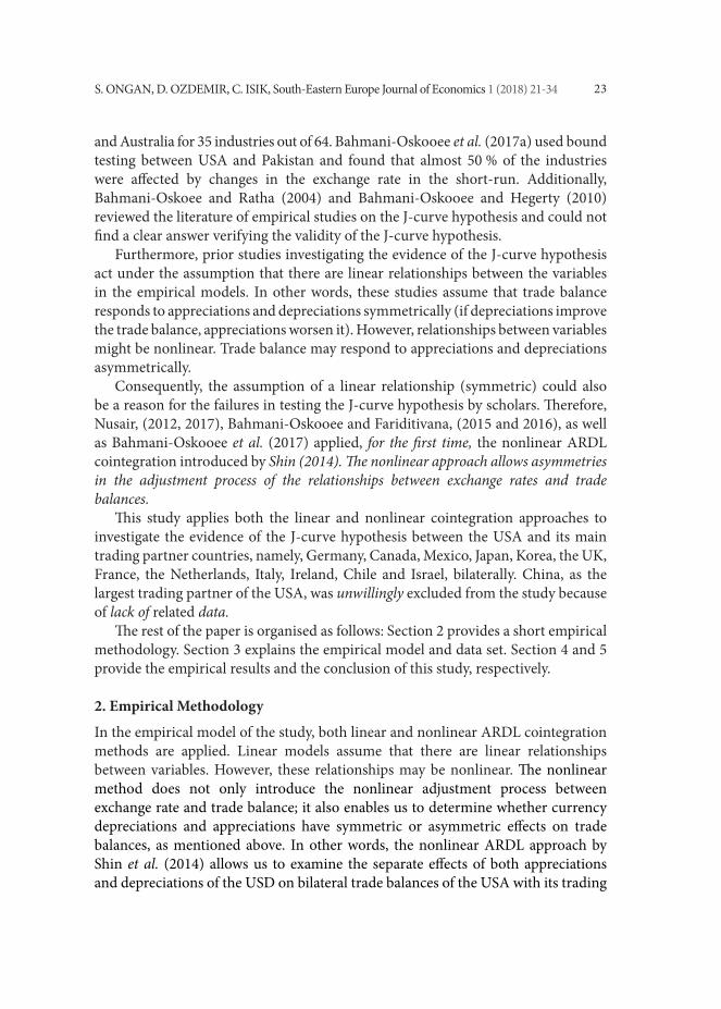
23S. ONGAN, D. OZDEMIR, C. ISIK, South-Eastern Europe Journal of Economics 1 (2018) 21-34

and Australia for 35 industries out of 64. Bahmani-Oskooee et al. (2017a) used bound testing between USA and Pakistan and found that almost 50 % of the industries were affected by changes in the exchange rate in the short-run. Additionally, Bahmani-Oskoee and Ratha (2004) and Bahmani-Oskooee and Hegerty (2010) reviewed the literature of empirical studies on the J-curve hypothesis and could not find a clear answer verifying the validity of the J-curve hypothesis. Furthermore, prior studies investigating the evidence of the J-curve hypothesis act under the assumption that there are linear relationships between the variables in the empirical models. In other words, these studies assume that trade balance responds to appreciations and depreciations symmetrically (if depreciations improve the trade balance, appreciations worsen it). However, relationships between variables might be nonlinear. Trade balance may respond to appreciations and depreciations asymmetrically. Consequently, the assumption of a linear relationship (symmetric) could also be a reason for the failures in testing the J-curve hypothesis by scholars. Therefore, Nusair, (2012, 2017), Bahmani-Oskooee and Fariditivana, (2015 and 2016), as well as Bahmani-Oskooee et al. (2017) applied, for the first time, the nonlinear ARDL cointegration introduced by Shin (2014). The nonlinear approach allows asymmetries in the adjustment process of the relationships between exchange rates and trade balances. This study applies both the linear and nonlinear cointegration approaches to investigate the evidence of the J-curve hypothesis between the USA and its main trading partner countries, namely, Germany, Canada, Mexico, Japan, Korea, the UK, France, the Netherlands, Italy, Ireland, Chile and Israel, bilaterally. China, as the largest trading partner of the USA, was unwillingly excluded from the study because of lack of related data. The rest of the paper is organised as follows: Section 2 provides a short empirical methodology. Section 3 explains the empirical model and data set. Section 4 and 5 provide the empirical results and the conclusion of this study, respectively.

2. Empirical Methodology

In the empirical model of the study, both linear and nonlinear ARDL cointegration methods are applied. Linear models assume that there are linear relationships between variables. However, these relationships may be nonlinear. The nonlinear method does not only introduce the nonlinear adjustment process between exchange rate and trade balance; it also enables us to determine whether currency depreciations and appreciations have symmetric or asymmetric effects on trade balances, as mentioned above. In other words, the nonlinear ARDL approach by Shin et al. (2014) allows us to examine the separate effects of both appreciations and depreciations of the USD on bilateral trade balances of the USA with its trading


partner countries. If appreciations of the USD affect trade balances of the country differently than depreciations do, this will imply asymmetric effects. Therefore, the nonlinear ARDL approach may provide more evidence than the linear approach in testing the hypothesis. The nonlinear ARDL approach also nests and extends the linear ARDL approach of Pesaran at al. (2001), as explained below.

3. Empirical Model and Data Set

Following previous studies (e.g. Bahmani-Oskooee and Fariditivana (2016), we adopt the following trade balance model:

(1)

Here, in the logarithmic form of the equation, it is assumed that the trade bal-ance (TB) of the US is a function of the incomes of the US and the US’s trading partner country i and the bilateral real exchange rate between the USD and the trading partner country i’s currency. In Eq. (1), is defined as the rate of US’s import from trading partner divided by its export to trading partner i. data were obtained from the IMF’s Direction of Trade Statistics. The are the US’s and trading partner country i’s Industrial Production Indices (as proxy of income). Data for this index were obtained from the database of the Federal Reserve Bank of St. Louis (FED). is the bilateral real exchange rate between the USD and trading partner country i’s currency. is defined as = (CPIUSA*NEXi/CPIi). NEXi is the nominal exchange rate defined as the number of units of trading partner i’s currency per USD. CPIUSA and CPIi are the Consumer Price Indices of the US and trading partner country i. The data of NEXi and CPI’s were obtained from the database of the Federal Reserve Bank of St. Louis (FED). The data used are monthly figures covering the period of 1991M1–2015M2. In Eqn.1, it is assumed that the sign of is to be positive in order to support the validity of the J-curve hypothesis between the US and its trading partner country. In other words, a decline in REX reflects real depreciation of the USD, increasing the US’s exports and improving the trade balance of the US (hence, the validity of the J-curve hypothesis). The sign of is assumed to be positive if an increase in income of the US leads to an increase in imports of the country. If an increase in income of the country is due to an increase in the production of substitute goods imported before, this may lead to less imports for the US yielding a negative sign for .Similarly, the sign of is also assumed to be positive or negative in the same way. Having defined the variables in Eqn. 1, we apply the linear ARDL cointegration approach of Pesaran et al. (2001), which considers both the short-run and long-run effects of the variables on a dependent variable. Therefore, we transform the model of Rose and Yellen (1989) in Eqn.1 to the linear ARDL approach of Pesaran et al. (2001) in Eqn.2.


In the linear model in Eqn.2, if short-run deterioration combines with long-run improvement on the trade balance (as the estimates of are negative or insignificant in the short-run and the estimate of normalized is positive and significant in the long-run) this will signify evidence of a J-curve according to the definition of Rose and Yellen (1989) (Bahmani-Oskooee and Fariditivana, 2016). In order to analyse the separate effects of depreciations and appreciations of the USD on the trade balances of the country, we apply the nonlinear approach introduced by Shin et al. (2014) and adapted by Bahmani-Oskooee and Fariditivana (2015 and 2016), as shown in the following model.

As seen in the equation above, appreciations (designated as POS) and depreciations (designated as NEG) of the USD are added, as additional variables, to Eqn.2. Thus Eqn.3 was derived from Eqn.2.The partial sums of POS and NEG changes in the USD are defined in the following form.

(4)

In the nonlinear model in Eqn.3, if the estimates of normalised long-run appreciation ( ) are significantly positive this will signify evidence of the J-curve hypothesis according to the definition of Bahmani-Oskooee and Fariditivana (2015 and 2016).

4. Empirical Results

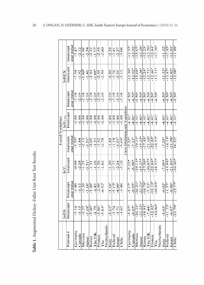
In this section of the study, we first present the empirical results of the linear ARDL cointegration approach of Pesaran et al. (2001). However, before this, we present the unit root test results of the Augmented Dickey-Fuller (ADF) for the stationary. ADF test results are reported in Table 1.

(3)

(2)

(4)


Tabl

e 1.

Aug

men

ted

Dic

key–

Fulle

r Uni

t Roo

t Tes

t Res

ults


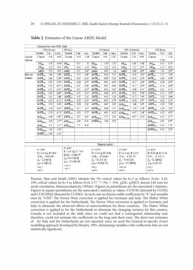
Test results show that some variables are stationary at their levels I (0) and some at their first differences I (1). But all are stationary at their first differences. Hence, we can apply the cointegration analysis for long-run relationships. To this aim, we apply the ARDL bounds testing, developed by Pasaran et al. (2001), using The critical values, tabulated by Pasaran et al. (2001) for a linear model of three exogenous variables with an unrestricted intercept and no trend, are 3.77 and 4.35 for the upper bounds and 2.72 and 3.23 for the lower bounds at the 10% and 5% significance levels, respectively. Hence, the empirical results of the linear models indicate that there are long-run relationships for all countries except Canada and Chile (neither is reported in Table 2), since their exceed the upper critical bounds value. Nevertheless, there is evidence of the J-curve hypothesis for the US with only Italy, the Netherlands, Mexico and France, since the estimates of ) are negative or insignificant in the short-run and estimates of normalised ( ) are positive and significant in the long-run. In other words, the J-curve hypothesis is supported since the depreciations in the USD deteriorate the US trade balance in the short-run and improve it in the long-run. The empirical results of the linear ARDL cointegration approach are reported in Table 2. On the other hand, the critical values tabulated by Pesaran et al. (2001) for a nonlinear model of four exogenous variables with an unrestricted intercept and no trend, are 3.52 and 4.01 for the upper bounds and 2.45 and 2.86 for the lower bounds at the 10% and 5% significance levels, respectively. Hence, the empirical results of the nonlinear models, reported in Table 3, indicate that there are long-run relationships for all countries since their exceed the upper critical bounds value. However, the evidence of the J-curve hypothesis for the USA is found with only Italy, Ireland, the Netherlands, Korea, Mexico, Japan, Israel and France, because the estimates of normalised long-run appreciation ( ) are significantly positive only for these countries. The empirical results of the nonlinear ARDL cointegration approach are reported in Table 3. Furthermore, the estimated ECM (error correction model) coefficients of both linear and nonlinear models are negative and significant for all countries except Germany. The speed of adjustment of the ECM in the nonlinear approach is higher than that of the ECM in the linear approach. To estimate the long-run asymmetric effects of appreciations and depreciations on the US trade balance, we apply the Wald test. The null hypothesis of long-run symmetry ( = ) is rejected implying that appreciations and depreciations have asymmetrical effects on the US trade balance with Canada, Ireland, Korea, Chile and Japan, since their long-run Wald statistics (WLR) are significant. Additional diagnostic tests are reported on relevant tables for the linear and nonlinear models.


Table 2. Estimates of the Linear ARDL Model

Pesaran, Shin and Smith (2001) tabulate the 5% critical values for k=3 as follows: Fcrit= 4.35, 10% critical values for k=3 as follows Fcrit 3.77. **: 5%, *: 10%. χ2SC, χ2HET, denote LM tests for serial correlation, Heteroscedasticity (White). Figures in parentheses are the associated t-statistics. Figures in square parentheses are the associated t-statistics p-values. CUSUM (denoted by CUSM) and CUSUMSQ (denoted by CUSM2). In each case we denote stable coefficients by “S” and unstable ones by “UNS”. The Newey-West correction is applied for Germany and Italy. The Huber White correction is applied for the Netherlands. The Newey-West correction is applied to Germany and Italy to eliminate the observed effects of autocorrelation for these countries. The Huber White correction is applied to for the Netherlands to eliminate the changing variance for this country. Canada is not included to the table since we could not find a cointegrated relationship and, therefore, could not estimate the coefficients in the long and short-runs. The short-run estimates of for Italy and the Netherlands are not reported, since we used the General-to-specific (Gets) modelling approach developed by Hendry 1995, eliminating variables with coefficients that are not statistically significant.


Table 2. Estimates of the Linear ARDL Model (continued)

Pesaran, Shin and Smith (2001) tabulate the 5% critical values for k=3 as follows: Fcrit= 4.35, 10% critical values for k=3 as follows Fcrit 3.77. ** : 5%, *:10%. χ2SC, χ2HET denote LM tests for serial correlation, Heteroscedasticity (White). Figures in parentheses are the associated t-statistics. Figures in square parentheses are the associated p-values. CUSUM (denoted by CUSM) and CUSUMSQ (denoted by CUSM2). In each case we denote stable coefficients by “S” and unstable ones by “UNS”.


Table 3. Estimates of the Nonlinear ARDL Model

Pesaran, Shin and Smith (2001) tabulate the 5% critical values for k=4 as follows: Fcrit= 4.01, 10% critical values for k=4 as follows Fcrit 3.52. **: 5%, *: 10%. χ2SC, χ2HET, denote LM tests for serial correlation, Heteroscedasticity (White). Figures in parentheses are the associated t-statistics. Figures in square parentheses are the associated p-values. CUSUM (denoted by CUSM) and CUSUMSQ (denoted by CUSM2). In each case, we denote stable coefficients by “S” and unstable ones by “UNS” WLR refers to the Wald test of long-run symmetry. The Newey-West correction is applied for Canada, Germany and Italy. The short-run estimates of and/or for Canada, Germany, Italy, Ireland, the Netherlands, the UK, Mexico and Israel are not reported, since we used the General-to-specific (Gets) modelling approach developed by Hendry 1995, eliminating variables with coefficients that are not statistically significant.


Table 3. Estimates of the Nonlinear ARDL Model (continued)

Pesaran, Shin and Smith (2001) tabulate the 5% critical values for k=4 as follows: Fcrit= 4.01, 10% critical values for k=4 as follows Fcrit 3.52. **: 5%, *: 10%. χ2SC, χ2HET denote LM tests for serial correlation, Heteroscedasticity (White). Figures in parentheses are the associated t-statistics. Figures in square parentheses are the associated p-values. CUSUM (denoted by CUSM) and CUSUMSQ (denoted by CUSM2). In each case, we denote stable coefficients by “S” and unstable ones by “UNS”. WLR refers to the Wald test of long-run symmetry. The short-run estimates of and/or for Canada, Germany, Italy, Ireland, the Netherlands, the UK, Mexico and Israel are not reported, since we used the General-to-specific (Gets) modelling approach developed by Hendry 1995, eliminating variables with coefficients that are not statistically significant.

The comparative empirical results of both linear and nonlinear ARDL cointegration approaches, in terms of validity of the J-curve hypothesis, are shown in Table 4. Table 4 clearly shows that while the nonlinear ARDL approach supports the evidence of the J-curve hypothesis for 8 countries, the linear approach supports this for only 4 countries. In other words, the nonlinear approach provides more evidence of the hypothesis than the linear approach. It should be noted that Bahmani-Oskooee and Fariditivana, in their recent study (2016), also found more evidence of the J-curve hypothesis with the nonlinear ARDL cointegration approach as compared to the linear approach. Canada, France, Germany, Italy, Japan and the UK are the countries our study has in common with the sample countries Bahmani-Oskooee


and Fariditivana (2016)’s study. When we compared the results of two studies in terms of these countries, we got some similar and some different findings. For instance, Italy and France are the countries supporting the evidence of the J-curve for the USA in both studies by both the linear and the nonlinear approaches. On the contrary, we found the evidence of a J-curve for the USA with Japan, whereas they could not find any such evidence for the same country. On the other hand, while we could not find any evidence of a J-curve for the USA with Germany, Canada and the UK, they found one for the same countries. Presumably, different findings for the same sample countries might result from the different time horizons and time frames used in both studies. While we used monthly data from 1991M1–2015M2, they used quarterly data from 1971Q1-2013Q3. Another reason for these differences might also arise from the different independent variables used in the two studies. While they used the GDP, we used the Industrial Production Index as the proxy of GDP, which allows researchers to make analyses using monthly data.

Table 4. The Validity of the J-curve Hypothesis by the Linear and Nonlinear Approaches

(+) denotes the validity of the J-curve hypothesis. (–) denotes the non-validity of thecurve hypothesis. (x) denotes no cointegration and, thereby, no estimated coefficients.


5. Conclusion

In conclusion, the US and its trading partner countries’ economic policy makers should take into consideration the validity or non-validity of the J-curve hypothesis and all these separate effects of both depreciations and appreciations of the USD in order to manage their countries’ sustainable trade balances, bilaterally. In addition, after the recent US election, the economic benefits of the North American Free Trade Agreement (NAFTA) have been scrutinised by the new presidential administration. Canada and Mexico, being members of the NAFTA, may experience some economic consequences depending on the USA’s actions with the agreement This is particularly true about Mexico, the country we found evidence for the J-curve hypothesis with the US from both linear and nonlinear ARDL approaches. Furthermore, apart from the evidence of the J-curve hypothesis, depreciations in the USD against to the Canadian Dollar deteriorate the US trade balance with this country both in the short- and the long-run. However, the same changes in the USD against the Korean Won improve the US trade balance with Korea in both the short- and the long-run. The empirical results of this study should also be considered on the basis of the Transatlantic Trade and Investment Partnership (TTIP) which is under ongoing negotiations between the US and the EU. The depreciations in the USD against to the Euro have significant positive effects on the USD trade balances with Italy, the Netherlands and France in the long-run. On the other hand, the depreciations and appreciations against to the British Pound do not have significantly negative or positive effects on the US trade balance with the UK, which is one of the largest trading partners of the USA in the EU and a country that is intending to leave the EU. This study also reveals the need for further empirical studies focused on the effects of depreciations and appreciations of the USD on the US and its trading partner countries’ bilateral trade balances. The results of these additional studies may be important for policymakers since the new US government has signaled a desire for changes in its bilateral international trade policy with its recent withdrawal from the proposed Trans-Pacific Partnership (TTP) trade deal between the US and Pacific Rim countries.

ReferencesBahmani-Oskooee, M. & T. J. Brooks., 1999, “Bilateral J-Curve between US and her Trading

Partners.” Weltwirtschaftliches Archive. 135, 156-165.Bahmani-Oskooee, M. & A. Ratha., 2004, “The J-Curve: a literature review.” Applied Economics,

36, 1377–1398.Bahmani-Oskooee, M., & A. Ratha., 2004, “Dynamics of the U.S. Trade with Developing

Countries.” Journal of Developing Areas 37(2): 1–11.Bahmani-Oskooee, M. & Y. Wang., 2007, “The J-Curve at the Industry Level: Evidence from Trade

between U.S. and Australia”, Australian Economic Papers, 46, 315-328.Bahmani-Oskooee, M. & S. W. Hegerty., 2010, “The J- and S-curves: A Survey of the Recent

Literature.” Journal of Economic Studies 37(6), 580–596.


Bahmani-Oskooee, M., Hegerty, S.W. & Hosny, A.S., 2015, “The effects of exchange-rate volatility on industry trade between the US and Egypt”, Economic Change and Restructuring, 48:93–117.

Bahmani-Oskooee, M. & Fariditavana, H., 2015, “Nonlinear ARDL Approach, Asymmetric Effects and the J-Curve,” Journal of Economic Studies, 43(3), 519-530.

Bahmani-Oskooee, M., Halicioglu, F & Hegerty, S.W., 2016, “Mexican bilateral trade and the J-curve: An application of the nonlinear ARDL model”, Economic Analysis and Policy, 50, 23-40.

Bahmani-Oskooee, M. & Fariditavana, H., 2016, “Open Economies Review, 27, 51-70.Bahmani-Oskooee, M., Halicioglu, F., & Mohammadian, A., 2017, “On the asymmetric effects of

exchange rate changes on domestic production in Turkey”. Economic Change and Restructuring, 1-16.

Bahmani-Oskooee, Iqbal, J. & Khan, S.U., 2017a, “Impact of exchange rate volatility on the commodity trade between Pakistan and the US”, Economic Change and Restructuring, 50(2), 161-187.

Census (2016). US Department of Commerce, Foreign Trade Statistics.Demirden, T. & I. Pastine., 1995, “Flexible Exchange Rates and the J-curve: An Alternative

Approach.” Economics Letters, 48, 373-377.Dickey, D. A., & W. A. Fuller., 1979, “Distribution of the Estimators for Autoregressive Time Series

with a Unit Root.” Journal of the American Statistical Association, 74, 427-431.FED (Federal Reserve Bank of St. Louis). 2016. Economic Research. https://research.stlouisfed.org/Hendry, D.F., 1995, Dynamic Econometrics: An Advanced Text in Econometrics, Oxford University

Press, Oxford.Hunt, B., Rebucci, A., 2005, “The US dollar and the trade deficit: what accounts for the late 1990s?”,

International Finance, 8 (3), 399–434.IMF (2017). Direction of Trade Statistics.Lerner, A., 1944, The Economics of Control, Macmillan, London.Mahdavi, S. & Sohrabian, A., 1993, “The exchange value of the dollar and the US trade balance: an

empirical investigation based on cointegration and Granger causality tests”, Quarterly Review of Economics and Finance, 33(4), 343–58.

Magee, S. P., 1973, “Currency contracts, pass through and devaluation.” Brooking Papers on Economic Activity, 1, 303–25.

Marwah, K. & Klein, L.R., 1996, “Estimation of J-curve: United Stated and Canada,” Canadian Journal of Economics, 29, 523-539.

Marshall, A., 1923, Money, Credit and Commerce, Macmillan, London.Narayan, Paresh, 2004, “New Zealand’s Trade Balance: Evidence of the J-Curve and Granger

Causality”, Applied Economics Letters, 11, 351-354.Nusair, A. S., 2012, “Nonlinear adjustment of Asian real exchange rates”, Economic Change and

Restructuring, 45(3), 221-246.Nusair, A. S., 2017, “The J-Curve phenomenon in European transition economies: A nonlinear

ARDL approach”, International Review of Applied Economics, 31(1), 1–27.Ongan, S.; Işik, C.; Özdemir, D. The Effects of Real Exchange Rates and Income on International

Tourism Demand for the USA from Some European Union Countries. Economies 2017 , 5 , 51.Pesaran, M.H., Y. Shin & R. J. Smith., 2001, “Bounds testing approaches to the analysis of level

relationships,” Journal of Applied Econometrics, 16, 289–326.Rose, A. K., & J. I. Yellen., 1989, “Is There a J-Curve?” Journal of Monetary Economics, 24, 53-68.Shin, Y, Yu, B., & Greenwood-Nimmo, M., 2014, “Modelling Asymmetric Cointegration and

Dynamic Multipliers in a Nonlinear ARDL Framework” Festschrift in Honor of Peter Schmidt: Econometric Methods and Applications, eds. by R. Sickels and W. Horrace: Springer, 281-314.

Shirvani, H., & B. Wilbratte., 1997, “The Relation Between the Real Exchange Rate and the Trade Balance: An Empirical Reassessment.” International Economic Journal, 11, 39-50.

Wassink, D. & Carbaugh, R., 1989, “Dollar-Yen Exchange rate effects on trade”, Rivista Int. Sci Econ. Com, 36(12), 1075–88.

TESTING THE J-CURVE HYPOTHESIS FOR THE … (2012, 2017), Bahmani-Oskooee and Fariditivana, (2015 and...

Documents

Transcript of TESTING THE J-CURVE HYPOTHESIS FOR THE … (2012, 2017), Bahmani-Oskooee and Fariditivana, (2015 and...