323

Charles University Center for Economic Research and Graduate Education

Academy of Sciences of the Czech Republic Economics Institute

Magdalena Morgese Borys

TESTING MULTI-FACTOR ASSET PRICINGMODELS IN THE VISEGRAD COUNTRIES

CERGE-EI

WORKING PAPER SERIES (ISSN 1211-3298) Electronic Version

Working Paper Series 323 (ISSN 1211-3298)

Testing Multi-Factor Asset Pricing Models in the Visegrad Countries

Magdalena Morgese Borys

CERGE-EI

Prague, March 2007

ISBN 978-80-7343-122-8 (Univerzita Karlova. Centrum pro ekonomický výzkum a doktorské studium) ISBN 978-80-7344-111-1 (Národohospodářský ústav AV ČR, v. v. i.)

1

Testing Multi-Factor Asset Pricing Models in the Visegrad Countries

Magdalena Morgese Borys*

CERGE-EI**

Abstract There is no consensus in the literature as to which model should be used to estimate the stock returns and the cost of capital in the emerging markets. The Capital Asset Pricing Model (CAPM) that is most often used for this purpose in the developed markets has a poor empirical record and is likely not to hold in the less developed and less liquid emerging markets. Various factor models have been proposed to overcome the shortcomings of the CAPM. This paper examines both the CAPM and the macroeconomic factor models in terms of their ability to explain the average stock returns using the data from the Visegrad countries. We find, as expected, that the CAPM is not able to do this task. However, a four-factor model, including factors such as: excess market return, excess industrial production, excess inflation, and excess term structure, can in fact explain part of the variance in the Visegrad countries’ stock returns.

Abstrakt V literatuře není konsensus ohledně toho, který model by měl být používán k odhadování výnosů z cenných papírů a kapitálových nákladů na rozvíjejících se trzích. Kapitálový model oceňování aktiv (KMOA), který je nejčastěji pro tento účel používán v rozvinutých trzích má slabou empirickou podporu a je pravděpodobné, že neplatí pro méně rozvinuté a méně likvidní rozvíjející se trhy. Různé faktorové modely byly navrženy, aby překlenuly nedostatky KMOA. Tato práce prozkoumává jak KMOA, tak makroekonomické faktorové modely ve světle jejich schopnosti vysvětlit průměrné výnosy z cenných papírů využívajíc data z Vyšegradských zemí. Zjišťujeme, v souladu s očekáváním, že KMOA není schopen tento požadavek naplnit. Nicméně, čtyřfaktorový model zahrnující faktory jako je tržní prémium, růst průmyslové produkce, inflace a struktura úrokových sazeb může ve skutečnosti vysvětlit část variance výnosů cenných papírů v zemích Vyšegradu. JEL Classification: G10, G 11, G12, G15, G31 Keywords: CAPM, macroeconomic factor models, asset pricing, cost of capital, Poland * I would like to express my gratitude to Petr Zemcik for useful comments and suggestions. I have also benefited from discussions with Evzen Kocenda and Jan Hanousek. **CERGE-EI is a joint workplace of the Center for Economic Research and Graduate Education, Charles University, and the Economics Institute of the ASCR, v. v. i. Address: CERGE-EI, P.O. Box 882, Politických vězňů 7, Prague 1, 111 21, Czech Republic E-mail: magdalena.borys@cerge-ei.cz

2

1. Introduction

Emerging markets have been quite extensively studied due to the large

interest of investors who view them as an attractive alternative to investing in

more developed markets. Emerging markets are typically characterized by

relatively higher returns, but also higher volatility of stock returns as compared

to the developed ones. However, there is no consensus in the literature as to

which model should be used to explain the returns in these markets and

estimate the cost of equity capital. The aim of this paper is to propose such a

model for the stock markets in Visegrad countries: the Czech Republic,

Hungary, Poland, and the Slovak Republic. More specifically, we will analyze

how different models perform in explaining the variations in stock returns on

the stock markets and which one of these models should be used to estimate

the cost of equity capital in this market.

Cost of equity capital is crucial information that is needed in order to

assess the investment opportunities and the performance of managed

portfolios. The cost of equity capital is used as a discount factor when

calculating the net present value (NPV) of the investment projects. In

principle, by using the net present value, investors want to verify whether the

payoff of the investment exceeds its cost1. The future payoffs expected from a

particular investment need to be discounted, so that they can be compared to

the costs of the investment that need to be incurred at the present time. In

1 A good discussion of the NPV methodology can be found in Brealey and Myers (1988). In

short, a simple NPV formula is as follows: NPV CC

rC

r= +

++

++0

1 221 1( )

.... ,

where C0 is the cash flow today (i.e. the cost of investment, a negative number), the C1 is the payoff from the investment one-period ahead, and r is the rate of return that investors demand for the delayed payment. This is the cost of capital.

3

developed markets, the capital asset pricing model (CAPM) is commonly used

by financial managers to calculate the cost of the equity capital, as well as to

assess the performance of managed portfolios, such as mutual funds (Fama

and French 2004). Graham and Harvey (2001) report that 75.5 percent of the

392 respondents to their survey use the CAPM to estimate the cost of equity

capital, which is then used to calculate the net present value (NPV) of the

investment projects, where the cost of equity capital is used as the discount

rate. The rationale behind using the cost of equity capital estimated by the

CAPM is the following: since the future payoffs from the investment are risky,

i.e. not certain, the rate of return used to calculate the NPV of this investment

should come from a comparably risky alternative investment opportunity. A

good candidate for such an alternative is investment in the stock market.

Therefore, the expected rate of return on the investment in the local stock

market, as predicted by the CAPM, can be used as a discount rate in

calculating the NPV of the investment project to be undertaken in a given

market. If the estimate of the firm’s beta coming from the CAPM is biased

upward it may lead to a rejection of profitable investments projects, i.e. when

the internal rate of return is not greater than the upward biased hurdle rate.

The CAPM formulated first by Sharpe (1964), Lintner (1965), and Black

(1972) describes the relationship between risk and expected return and is

used to price risky securities. A very clear and intuitive link between an asset’s

risk in relation to the risk of the overall market and an asset’s expected return

is one of the main advantages of the CAPM and is key to understanding its

widespread use. There are, however, also some caveats to using the CAPM.

Specifically, there are many empirical studies showing that the CAPM in its

4

classical version does not hold for the period of the second half of the

twentieth century even in developed markets. While Black, Jensen and

Scholes (1972) and Fama and Macbeth (1973) find that the CAPM holds for

the 1926-1968 period, more recent studies of the period 1960’s-2000’s find

otherwise. Among the first studies to report the disappearance of the simple

relation between the asset’s risk and the average return, as predicted by

CAPM, were Reinganum (1981) and Lakonishok and Shapiro (1986). Fama

and French (1993) propose a multi-factor model, which includes factors

related to the firm’s size and firm’s book value. This model performs better

than the classical CAPM and they argue that stock risks are multidimensional

and therefore the addition of other factors improves the CAPM power to

explain the average stock returns.

Fama-French factors (FF factors) are the most commonly used in the

literature as they turned out to be the most successful empirically. In order to

obtain these factors the stocks need to be grouped into portfolios on the basis

of the firm’s size, as well as firm’s book-to-market value2. In addition, factors

related to some macro variables have also proven to be able to explain the

variation in stock returns. Chen, Roll and Ross (1986) test whether additional

sources of risk such as innovations in macroeconomic variables are priced in

the stock market. They find that indeed some of these variables do affect the

stock market. The significantly priced macro variables include: the spread

between long- and short-term interest rates, expected and unexpected

inflation, industrial production, and the spread between high- and low-grade 2 Specifically, they advocate the multi-factor model with the following three factors: market return, the return on small stocks minus the return on the big stocks (SMB), and the return on stocks with high book to market ratio minus the return on stocks with low book to market ratio (HML).

5

bonds. Moreover they argue that neither the market portfolio, nor aggregate

consumption is priced separately. Given the widespread of factor models and

they empirical success, we will also propose and test a factor model that could

be used to explain the stock returns in the stock markets of Visegrad countries

and allow to estimate the cost of equity in these markets, subject to data

limitations.

The CAPM, as well as most factor models, include the overall market

return as a factor. Market portfolio by definition should contain all the traded

and non-traded assets and so in practice the composition of such true market

portfolio is unknown. Therefore, the researchers use various proxies for the

market portfolio that most often consist of traded stocks. Roll (1977) argued

that violations of the CAPM that are found in empirical works might be due to

the choice of the market portfolio. Low and Nayak (2005) show that the choice

of market portfolio is irrelevant for the validity of the CAPM. They conduct

comprehensive simulations to show that if the CAPM is found to hold using

one proxy for the market portfolio, it holds for all the alternative proxies. More

importantly, this is also true in an opposite case; if the CAPM does not hold for

one of the specifications, it does not hold for any other, where different proxies

for market portfolio are used. Similarly, Bartholdy and Peare (2003) show that

the Fama-Macbeth procedure (FMB) results in an unbiased estimate of the

expected returns even though a proxy is used for the market portfolio.

Moreover, they argue that unbiased results are obtained independently from

the proxy used as long as the FMB procedure is executed correctly.

As discussed above, the classical CAPM model does not always hold

in practice when used to analyze the markets in developed countries. The

6

markets in emerging markets, including the stock markets in Visegrad

countries, are less efficient and less liquid compared to the developed

markets and so it is likely that the CAPM model, especially in its classical

formulation, may not be suitable for estimating the cost of capital for these

economies. Harvey (1995) argues that the emerging markets are

characterized by low betas and the CAPM model is not able to capture the

relationship between the stock returns in these countries and the market

portfolio. Based on this finding there are several studies that analyze various

factors that influence the stock returns in the emerging markets and propose

models suitable for estimating the cost of capital in these markets. Erb,

Harvey, and Viskanta (1995, 1996) find that country credit ratings are

significantly related to stock returns, and they propose a model based on

these indices. Similarly, Harvey (2004) argues that the country risk rating from

the International Country Risk Guide impacts the expected returns in

emerging markets and so he incorporates these indices in his version of the

CAPM model.

The issue of the relative integration of the emerging markets with the

global markets and its implications on the stock returns in these markets has

been central in the literature. Bekaert and Harvey (1995) argue that the

integration of the emerging markets with the global markets has been a

dynamic process and therefore also the cost of capital should be allowed to

vary over time as the relative measure of the integration with global markets

changes. In a more recent paper, Bekaert and Harvey (2000) develop a

model, in which dividend yields are used as a measure of the equity cost of

capital. They find that the cost of capital declines as the emerging markets

7

become more integrated with global markets. In one of the few papers that

study the markets in Central and Eastern Europe (CEE), Sokalska (2001)

finds that stock prices of the Czech Republic, Hungary and Poland move

together. She argues that local macroeconomic fundamentals are of relatively

small importance in those markets and that the key factors influencing the

movements of stock prices are exogenous. Namely, she claims that it is the

flow of foreign portfolio capital that can be traced to affect the movement of

stock prices in those markets. De Jong and de Roon (2001) link the issue of

time varying market integration with expected returns in emerging markets.

They develop a model, in which expected returns depend on the degree of

market segmentation, measured as a ratio of assets in a given market that

cannot be traded by foreign investors. Given that the degree of segmentation

changes over time, they allow the expected returns to also vary with time.

Using data from 30 emerging markets, including the Visegrad countries, de

Jong and de Roon provide evidence that the market segmentation has a

significant effect on the expected returns. They find in line with the theory that

increasing market integration (or decreasing market segmentation) leads to

lower expected returns and hence lower cost of capital.

There are some important data and methodological issues that need to

be addressed in the Visegrad countries. First, the data available is of relatively

short time span, which may influence the plausibility of our results. Second,

there is a limited number of stocks traded on these stock exchanges3, which

makes some of the commonly used portfolio techniques not feasible. Taking

these considerations into account, we used the FMB procedure to estimate

3 The variability in the number of stocks traded in the sample is given in Table I and Table II.

8

our models. This procedure is extensively used by the researchers to estimate

and test the single- and multi-factor models’ predictions. It gives unbiased

estimates even when there is correlation between observations on different

firms in the same year. It also accounts for a variation coming from both time-

series and cross-section regressions, which is especially important when

there is a limited number of observations, as it is the case with the Visegrad

countries’ data.

First, we estimated the CAPM by the FMB procedure to see how this

model performs in stock markets of Visegrad countries. We found that we

could not reject the classical CAPM in Hungary and in Slovakia since the

constant term was not statistically different from zero. However, also the slope

coefficients on the excess market return were not significant, indicating that

they local market alone was not able to explain the variation in stock returns in

these markets. For the Czech Republic and Poland we could reject the CAPM

since the constant terms were significantly different from zero, which indicated

the presence of pricing errors in this model specification.

Given these results we proceeded with the estimation of the factor

model. Due to data limitations, we were not able to construct the FF factors.

Therefore, we developed a model, in which the macroeconomic factors are

used. We extended the classical CAPM by adding the following three factors:

industrial production, inflation, and the term structure. Similarly to the CAPM,

this four-factor model was not sufficient to explain the variation in stock

returns on these markets, although it had some explanatory power in Poland

and in Hungary. Specifically, both in Poland and in Hungary the term structure

was significantly priced, indicating that this factor is able to explain part of the

9

variation in the average stock returns in these markets. In Poland inflation was

similarly a priced factor. The presence of pricing errors was detected in the

model for Czech Republic, Poland, and the Slovak Republic since the

constant terms were significant. In addition, we estimated alternative factor

models, which included other variables that we believe may be important in

Visegrad countries. Some of the additional factors, which turned out to be

significantly priced, included money, exchange rate, and German industrial

production.

Given mixed results stemming from macroeconomic factor models we

proceeded to estimate other multi-factor models, in which we used the

principal components as factors. For all Visegrad countries we estimated a

four-factor model with excess market return and three first principal factors. In

case of Poland, all four factors were significant, though the constant term was

still significant, indicating the presence of pricing errors. The third principal

factor was also significant for Slovakia but none of the factors turned out to be

significant in other countries. Keeping in mind that there may be some errors-

in-variables present in the FMB estimation, we decided to proceed with an

alternative estimation method as a robustness check. The method that

appears to be the most suitable for this purpose is the General Method of

Moments (GMM), in which both time series factor sensitivities (betas) and

time-varying cross sectional loadings on the risk premia (gammas) are

estimated simultaneously, instead of two-stage estimation procedure in FMB.

We were able to obtain these alternative estimates only for Poland since we

10

run into empirical problems with data from other Visegrad countries4. The

results for Poland confirm that FMB estimation causes the estimates of

coefficients to be somewhat biased. The estimates obtained using the GMM,

an estimation method free of errors-in-variables problem, changed in the way

that is in line with literature on the errors-in-variables: estimates of slope

coefficients (gammas) increased and estimates of constant term decreased,

resulting in many factors that were previously not priced significantly turning

significant and resulting in constant terms loosing their significance.

This paper is organized as follows. In Section 2 we discuss CAPM and

factor models in greater detail, as well as the testing procedures. In Section 3

we introduce the data and discuss some its limitations that make the use of

some standard techniques impossible. Section 4 contains the empirical results

from testing the CAPM and factor models in the Visegrad countries. In Section

5, we briefly summarize the findings of this paper and suggest some direction

for further research.

2. Methodology

The main objective of this paper is to point to suitable asset-pricing

model that could be used to estimate the cost of equity capital in the Visegrad

countries. The first candidate is the Capital Asset Pricing Model (CAPM).

According to this classical model specification, the expected return on the

security or on the portfolio of securities should be equal to the risk-free rate

plus a risk premium, which consists of the portfolio's beta multiplied by the

4 The residual variance-covariance matrices for the Czech Republic, Hungary and Slovakia turned were not positive definite, hence it was not possible to invert these matrices to obtain the estimates.

11

expected excess return of the market portfolio (return on the market portfolio

minus the risk free rate). A classical, one-factor CAPM looks as follows:

( )E r -r = E r rit tf

i tm

tf( ) ( )β − , (1)

where E(rit) is the expected i-th stock return (i=1….N), rtf is the risk-free rate,

and E rtm( ) is the expected market return. This model can be empirically tested

using the following regression equation:

( )r -r = r rit tf

i im

tm

tf

itα β ε+ − + (2)

where rit - rtf is the excess market return on i-th stock, rmt is the market return

αi is the constant term, βim is the coefficient on the excess market return for

each of the i stocks, and εit is the error term. According to the CAPM

prediction, the constant term, αi , should be statistically insignificant (i.e. equal

to zero) for each of the i stocks. If this is the case, the pricing errors are zero

and the CAPM is said to hold empirically. In addition, the slope coefficient,

βim , should be significantly different from zero, indicating that the excess

market return is indeed priced by the stock market, i.e. it helps to explain the

variation in the stock returns. Moreover this coefficient, which represents the

measure of one stock’s risk as compared to the risk of the overall market,

should vary among the stocks.

We also considered an extension of the classical CAPM - a multi-factor

model. Suppose there are k-factors that are believed to influence the stock

12

returns in a given market. The k-factor model can be tested by using the

following regression equation:

( ) ( ) ( )r -r = r r r rit tf

i im

tm

tf

i t iK

tK

itα β β β ε+ − + + + +2 2 ..... (3)

where rtm

is a local index return, rtk is the k-th factor return (k=2…K), rit is the

i-th stock return, rtf is the risk-free rate, αi is the constant term, and εit is the

error term. Similarly to the CAPM, this multi-factor model predicts that the

constant terms, αi , should be insignificant and the slope coefficients, βim and

βik , should be significantly different from zero. As discussed, these factors

may include Fama-French factors or other factors, including macroeconomic

variables or the principal factors obtained by the principal component analysis.

In the literature one can find several ways of testing the capital asset

pricing models. They can be divided into the following three categories: tests

involving time-series regressions, tests involving cross-section regression,

and the tests involving a combination of the above5. One of the most widely

used methods is the FMB procedure, which combines the time series and the

cross section regressions. Suppose we have N firms returns for any given

month t, Rt. In the first stage we regress the excess stock return on the

excess market return and other k-factors in order to obtain the CAPM cross-

section betas, $βim and $βi

k , where i is a firm’s subscript (i =1….N), m stands

for the market return, and k is a factor’s subscript (k=2….K). In the second

5 A detailed discussion of these various methods can be found in Cuthbertson and Nitzsche (2001).

13

stage we run the following cross-section Ordinary Least Squares (OLS)

regression for any single month t6:

Rim

im k

ik

i= + + +γ γ β γ β η0$ $ (4)

where Ri=(R1, R2,…., RN) is a Nx1 vector of cross-section excess monthly

stock returns

$βim and $βi

k are NxK matrices of CAPM betas (obtained in the first

stage

regressions)

γ m and γ k are vectors of cross-section coefficients for each of the

k- factors

γ 0 is a scalar and an estimate of intercept

ηi is a Nx1 vector of cross-section error terms

Then we repeat this regression as in (4) for each month t=1,2,…T and

obtain T estimates of γ 0 , γ m and γ k . Finally, the time-series estimates of

these parameters are tested to see if: ( )E γ 0 0= (i.e. pricing errors are zero),

( )E mγ > 0 (i.e. positive risk premium on the excess market return), and

( )E kγ > 0 (i.e. positive risk premium on betas for each of the k factors).

Assuming the returns are iid and normally distributed the following t-statistic is

used:

6 This exposition of the FMB procedure is based on Cuthbertson and Nitzsche (2001) p. 193.

14

tk

kγ

γσ γ

=$

( $ ) , where ( )σ γ γ γ2

1

211

( $ ) ( $ $ )k k kt

T

T T=

−−

=∑ (5)

Similarly, one can obtain t-statistics tγ for γ m and γ 0 and test all of the

CAPM restrictions.

There is one important caveat to the FMB approach. Since the

estimates of betas, $βim and $βi

k , obtained in the first stage regressions may

be measured with error, we may encounter the ‘errors-in-variables’ problem in

the second stage regressions. Specifically, if the estimates of $βim and $βi

k that

we use in the second stage regressions contain measurement error, then the

estimates γ m and γ k will be biased7. The most common approach to

minimizing this problem is to group the stocks into portfolios8 and estimate the

portfolio betas instead of the stock betas in the first stage regression. Then, in

the second stage, the average excess return r rif− for each of the stocks is

regressed on the appropriate portfolio beta. This approach reduces the

measurement error but it does not completely resolve this problem since it still

uses betas estimated in the first step in the regressions in the second step.

Using portfolios rather than individual stocks can, however, improve the

estimates mainly due to utilizing the portfolios’ betas rather than the individual

stocks’ betas, which may contain structural breaks. Due to limited number of

companies listed on the Visegrad stock exchanges, there is not enough

observations at any given point of time to form portfolios of individuals stocks.

7 In the least squares regressions, the errors-in-variables are likely to cause the estimates of the slope coefficients to be biased downward and the estimate of a constant term to be biased upward. 8 The portfolios can be formed based on the size, beta or book-to-market ratio of individual stocks obtained from running the time-series regressions.

15

Instead, we proceed with alternative estimation method that allows for a

simultaneous estimation of betas and gammas, and therefore avoids the

errors-in-variable problem altogether. Cochrane (2005) shows that it is

possible to use the GMM estimation in this fashion. More specifically, in case

of single factor he proposes to combine the moment conditions used to

estimate betas and gammas in the following way:

( )( )( )[ ]

( ) ⎥⎥⎥

⎦

⎤

⎢⎢⎢

⎣

⎡=

⎥⎥⎥

⎦

⎤

⎢⎢⎢

⎣

⎡

−−−−−

=000

βγβαβα

ett

et

te

t

REffRE

fREbgT (6)

In this system there are N(1+K+1) moment conditions since for each asset N

we have one moment condition for the constant, K moment conditions for K

factors and one moment condition that allows to estimate the lambdas (asset-

pricing model condition).

To summarize, in this paper we estimated several alternative models,

including the classical CAPM, macroeconomic factor models and principal

factor model using the two alternative estimation methods: the FMB and the

GMM. One of the main advantages of FMB estimation procedure is that it

uses all the information available for a given data point, accounting for

variation coming from both sources: time-series and cross-section. Given

relatively short time spans of data available for the stock markets in Visegrad

countries, it is key to be able to utilize all the available data points to their

maximum. This procedure is, however, prone to errors-in-variables problem

due to a two-stage estimation. In order to account for this problem, we

obtained alternative estimates for Poland using the GMM one-step procedure,

16

which allowed us to assess the potential importance of the errors-in-variables

in our models. Unfortunately, we were not able to obtain similar estimates for

other Visegrad countries due to the variance-covariance matrices not being

positive definite, hence not invertible.

3. Data

Data on individual stocks, as well as local market indices needed in

order to test the validity of the classical CAPM in Visegrad countries were

obtained from Wharton Research Data Services. Other data was obtained

from IMF’s International Financial Statistics Database, national banks’ and

minister of finance’ websites. The summary of these variables is presented in

Table I.

17

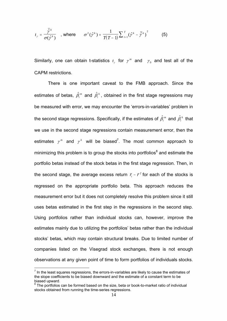
Table I

Summary Statistics for Variables Used in the CAPM Regressions

Sample mean, standard deviation, maximum and minimum values are reported for the variables used in the CAPM regression. These statistics are reported for the cross sectional distribution, where the number of firms varies from 8 to 74 depending on the country. All the variables represent monthly returns in local currency. Stock_rt stands for stock return, market_rt is the local market return, and tbill is a monthly return on short term government securities.

As argued, the classical, one-factor CAPM does not always hold

empirically and therefore various multi-factor models have been proposed in

the literature. FF factors are the most commonly used in the literature as they

turned out to be the most successful empirically. In order to obtain these

factors the stocks need to be grouped into portfolios on the basis of the firm’s

Variable/ Country

Mean Std. Dev. Min. Max.

Czech Republic 4660 obs; 1994:02 – 2003:02 No of Companies: 9-74

stock_rt -.0068 .1654 -.6325 1.535 market_rt -.0094 .0732 -.2059 .1699 Local t-bill .0074 .0025 .0021 .0129 Hungary 1867 obs; 1993:01-2003:02 No of Companies: 12-18

stock_rt .0181 .1760 -.5707 2.260 market_rt .0196 .1088 -.3582 .4583 Local t-bill .0151 .0063 .0044 .0283 Poland 2937 obs; 1994:02-2003:02 No of Companies: 12-35

stock_rt .0050 .1569 -.9962 1.895 market_rt .0057 .1055 -.3233 .3970 Local t-bill .0142 .0047 .0049 .0252 Slovak Republic 1200 obs; 1996:08-2003:02 No of Companies: 8-20

stock_rt .0427 1.008 -.9810 26.78 market_rt -.0097 .0759 -.1709 .3079 Local t-bill .0119 .0044 .0050 .0217

18

size, as well as firm’s book-to-market value. Due to a limited number of stocks

traded in the stock markets of Visegrad countries, the portfolio grouping is not

possible.

Therefore, in this paper a second best approach is used, namely the

macroeconomic factor model. It has been noted that observable economic

time series like inflation and interest rates can be used as measures of

pervasive and common factors in stock returns. Chen, Roll and Ross (1986)

argue that the stock prices can be expressed as expected discounted

dividends:

kcEp )(

= (6)

where c is the dividend stream and k is the discount factor. From this it can be

deducted that the economic variables that influence discount factors as well

as expected cash flows will also influence the expected returns. Chen, Roll

and Ross (CRR) use the following factors: industrial production growth, a

measure of unexpected inflation, changes in expected inflation, the difference

in returns on low grade corporate bonds and long-term government bonds

(risk premia), the difference in returns on long-term government bonds and

the short-term Treasury bills (term structure), changes in real consumption,

and oil prices. In our factor model, similarly to CRR, we included a monthly

industrial growth and the term structure. In contrast to CRR, we did not

include two inflation variables in order to avoid likely correlations between

them. Instead, we used only the monthly inflation. Since there is no time-

series data on corporate bond grading in Visegrad countries, we did not

incorporate any measure of risk premia in our model. CRR find that changes

in consumption and oil prices are not significantly related to the stock returns.

19

Therefore, we did not include these two factors in our specification. To

summarize, in our baseline factor model we used the following four factors:

market return, monthly growth rate of industrial production, inflation, and term

structure. Changes in the level of industrial production affect the real value of

cash flows. In addition, a direct link between the returns and production is

specified in the business cycle models. Inflation influences the nominal value

of cash flows, as well as the nominal interest rate. Finally, the discount rate is

affected by the changes in the term structure spreads between different

maturities. In addition, we estimated alternative factor models, which included

variables that we believe may be important in Visegrad countries. The

additional variables included: exchange rate, German industrial production,

money, and exports. Given that all these countries are relatively small, open

economies, the fluctuations in exchange rate, exports and money base are

likely to have strong impact on other macroeconomic variables. The economic

situation in Germany (proxied by its industrial production), one of the most

important trading partners for the Visegrad countries, may have a significant

impact on the economies of these countries and therefore may also influence

their stock markets. The time series of all these additional variables were

obtained from the IMF International Financial Statistics Database. The

summary of these variables is presented in Table II.

In order to overcome the limitations of factor models with respect to the

small number of variables that can be used in the estimation, we employed

the principal component analysis to extract the main factors driving the

economies of the Visegrad countries. This method is mainly used for

forecasting purposes. It is based on the principle that there are a few forces

20

driving the dynamics of all macroeconomic series. Since these forces are

unobservable they need to be estimated from a large number of economic

time series. Given the still transitionary character of the Visegrad stock

markets, as well as the limited span of data available, principal component

analysis may be very useful for explaining the stock returns in these countries.

The list of variables used to obtain the principal factors is included in the

Appendix. The first three principal factors, which explained most of the

variance of the average stock returns, were then used as the factors in the

alternative multi-factor model (principal factor model). In addition, the same

number of factors as the baseline multi-factor model, allowed a direct

comparison of the performance of these two models. The summary statistics

of the three first principal factors used in the principal factor model are

presented in Table III.

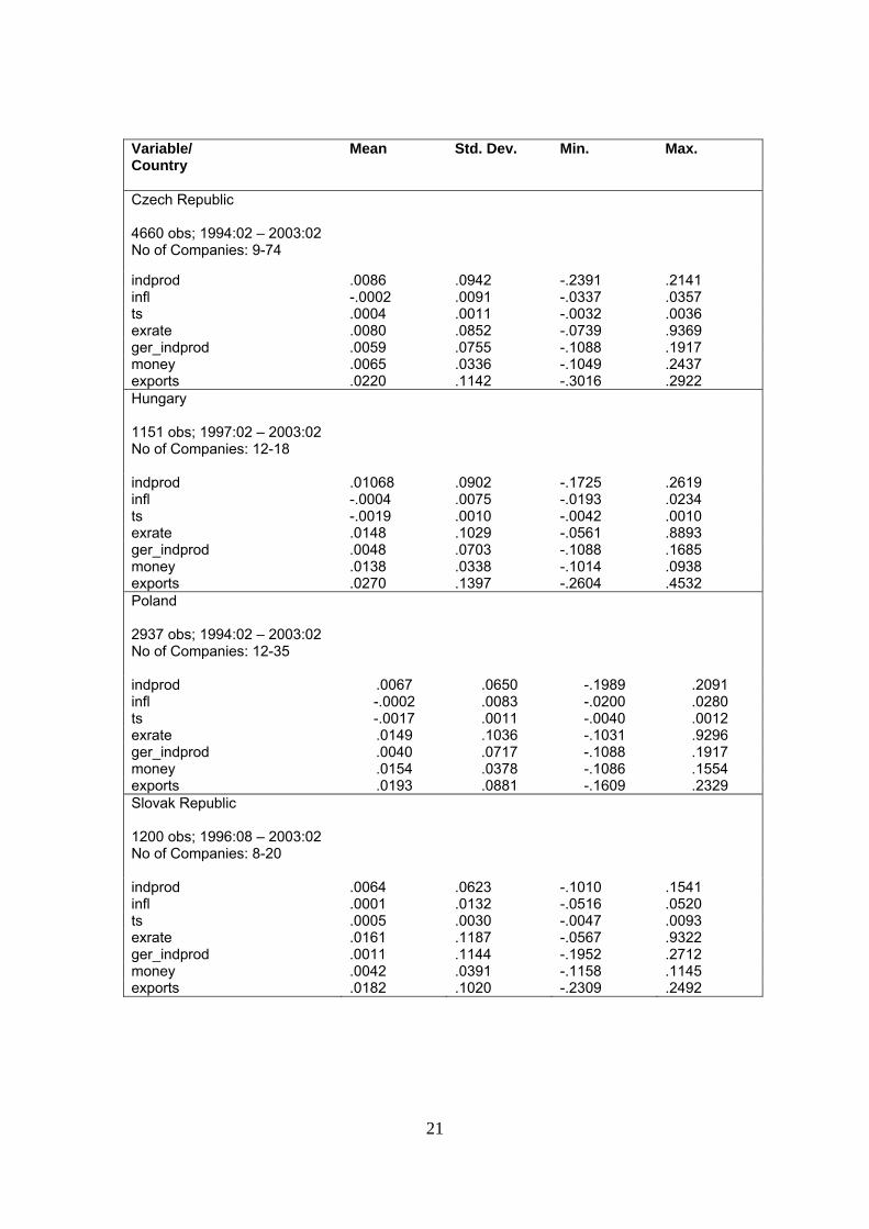
Table II

Summary Statistics for the Additional Variables Used in the Factor Model Regressions

Sample mean, standard deviation, maximum and minimum values are reported for the additional variables used in the multi-factor model regression (market return, stock return and local t-bill statistics are reported in Table I). These statistics are reported for the cross sectional distribution, where the number of firms varies from 8 to 74 depending on the country. All the variables represent monthly returns or growth rates in local currency. The time series for term structure was obtained by subtracting a monthly return on treasury bills from a monthly return on long-term government bonds. In the subsequent statistical analysis CPI inflation and term structure used in first differences since their original time series contain unit roots. Indprod stands for monthly industrial production growth rate, infl represents monthly growth in inflation, ts is a term structure, exrate is a monthly appreciation/depreciation of the national currency as compared to euro, ger_indprod stands for a monthly industrial production growth in Germany, money represents monthly growth in M1, and exports is a monthly growth in exports.

21

Variable/ Country

Mean Std. Dev. Min. Max.

Czech Republic 4660 obs; 1994:02 – 2003:02 No of Companies: 9-74

indprod .0086 .0942 -.2391 .2141 infl -.0002 .0091 -.0337 .0357 ts .0004 .0011 -.0032 .0036 exrate .0080 .0852 -.0739 .9369 ger_indprod .0059 .0755 -.1088 .1917 money .0065 .0336 -.1049 .2437 exports .0220 .1142 -.3016 .2922 Hungary 1151 obs; 1997:02 – 2003:02 No of Companies: 12-18

indprod .01068 .0902 -.1725 .2619 infl -.0004 .0075 -.0193 .0234 ts -.0019 .0010 -.0042 .0010 exrate .0148 .1029 -.0561 .8893 ger_indprod .0048 .0703 -.1088 .1685 money .0138 .0338 -.1014 .0938 exports .0270 .1397 -.2604 .4532 Poland 2937 obs; 1994:02 – 2003:02 No of Companies: 12-35

indprod .0067 .0650 -.1989 .2091 infl -.0002 .0083 -.0200 .0280 ts -.0017 .0011 -.0040 .0012 exrate .0149 .1036 -.1031 .9296 ger_indprod .0040 .0717 -.1088 .1917 money .0154 .0378 -.1086 .1554 exports .0193 .0881 -.1609 .2329 Slovak Republic 1200 obs; 1996:08 – 2003:02 No of Companies: 8-20

indprod .0064 .0623 -.1010 .1541 infl .0001 .0132 -.0516 .0520 ts .0005 .0030 -.0047 .0093 exrate .0161 .1187 -.0567 .9322 ger_indprod .0011 .1144 -.1952 .2712 money .0042 .0391 -.1158 .1145 exports .0182 .1020 -.2309 .2492

22

Table III

Summary Statistics for the Factors Obtained from the Principal Component Analysis

Sample mean, standard deviation, maximum and minimum values are reported for the first three leading factors obtained from the principal component analysis. These statistics are reported for the cross sectional distribution, where the number of firms varies from 8 to 74 depending on the country.

Principal components

Mean Std. Dev. Min. Max.

Czech Republic 4660 obs; Aug 1996 – Feb 2003

No of Companies: 9-74

Pc 1

.2753125 1.572405 -3.939665 4.25058

Pc 2

.0906176 1.408384 -2.782753 2.872529

Pc 3

-.2358732 1.288445 -4.73856 6.000414

Hungary 1151 obs; Feb 1997 – Feb 2003

No of Companies: 12-18

Pc 1

.6208512 1.669118 -3.753944 4.502163

Pc 2

.5866697 1.451879 - 2.114966 4.119454

Pc 3

.4055286

1.40061 -2.040843 4.104701

Poland 2937 obs; 1994:02 – 2003:02

No of Companies: 12-35

Pc 1

1.178026 1.753528 -2.95811 10.70719

Pc 2

.1220507 2.364502 12.76142 3.589532

Pc 3

-.109039 2.117285 -8.281503 9.921389

Slovak Republic 983 obs; May 1999 – Dec 2002

No of Companies: 8-20

Pc 1

.0111274 3.714044 -13.02892 13.76797

Pc 2

.0928082 3.166589 -7.305079 8.128183

Pc 3

.0319989 2.321968 -7.864149 5.494952

23

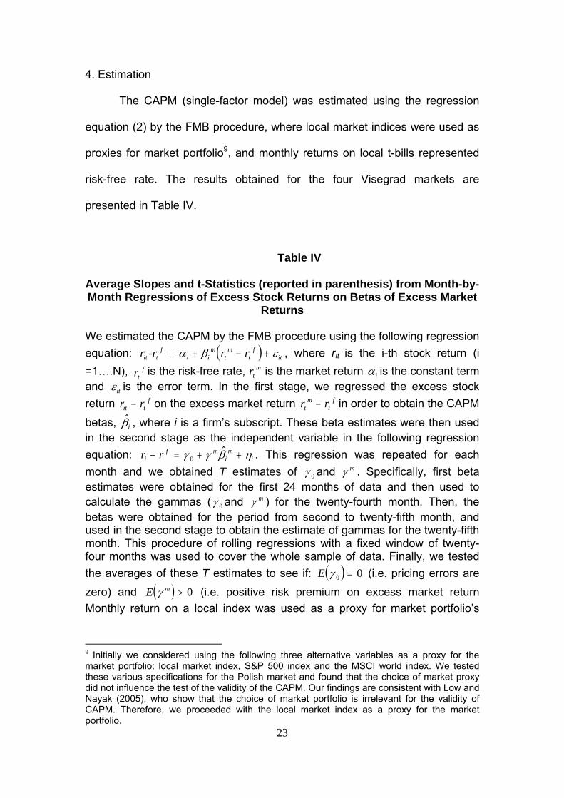
4. Estimation

The CAPM (single-factor model) was estimated using the regression

equation (2) by the FMB procedure, where local market indices were used as

proxies for market portfolio9, and monthly returns on local t-bills represented

risk-free rate. The results obtained for the four Visegrad markets are

presented in Table IV.

Table IV

Average Slopes and t-Statistics (reported in parenthesis) from Month-by-Month Regressions of Excess Stock Returns on Betas of Excess Market

Returns

We estimated the CAPM by the FMB procedure using the following regression equation: ( )r -r = r rit t

fi i

mtm

tf

itα β ε+ − + , where rit is the i-th stock return (i =1….N), rt

f is the risk-free rate, rtm

is the market return αi is the constant term and εit is the error term. In the first stage, we regressed the excess stock return r rit t

f− on the excess market return r rtm

tf− in order to obtain the CAPM

betas, $βi , where i is a firm’s subscript. These beta estimates were then used in the second stage as the independent variable in the following regression equation: r ri

f mim

i− = + +γ γ β η0$ . This regression was repeated for each

month and we obtained T estimates of γ 0 and γ m . Specifically, first beta estimates were obtained for the first 24 months of data and then used to calculate the gammas (γ 0 and γ m ) for the twenty-fourth month. Then, the betas were obtained for the period from second to twenty-fifth month, and used in the second stage to obtain the estimate of gammas for the twenty-fifth month. This procedure of rolling regressions with a fixed window of twenty-four months was used to cover the whole sample of data. Finally, we tested the averages of these T estimates to see if: ( )E γ 0 0= (i.e. pricing errors are

zero) and ( )E mγ > 0 (i.e. positive risk premium on excess market return Monthly return on a local index was used as a proxy for market portfolio’s

9 Initially we considered using the following three alternative variables as a proxy for the market portfolio: local market index, S&P 500 index and the MSCI world index. We tested these various specifications for the Polish market and found that the choice of market proxy did not influence the test of the validity of the CAPM. Our findings are consistent with Low and Nayak (2005), who show that the choice of market portfolio is irrelevant for the validity of CAPM. Therefore, we proceeded with the local market index as a proxy for the market portfolio.

24

return and monthly return on a local t-bill was used as a risk-free rate. *, **, *** indicate significant difference at the 10, 5, and 1 percent levels, respectively. Country Sample Local index

(γ m ) Constant

(γ 0 )

Czech Republic

Feb 1994 - Feb 2003 0.0026 (0.3117)

-0.0141 (-2.8732***)

Hungary

Jan 1993 - Feb 2003 0.0113 (0.7577)

-0.0109 (-0.8286)

Poland

Jan 1993 - Feb 2003 0.0106 (0.9052)

-0.0173 (-2.1076**)

Slovak Republic

Aug 1996 - Feb 2003 0.0114 (0.3225)

0.0207 (0.8865)

These results indicate that the CAPM should not be rejected for

Hungary and the Slovak Republic, as none of the constant terms was

statistically different from zero. However, also the coefficients gammas (γ m )

were not statistically different from zero, which implies that the market return

was not priced. Results for the Czech Republic and Poland indicated that the

CAPM should be rejected, as the constant terms were significantly different

from zero, which indicates the presence of pricing errors in this model

specification. This result is not surprising and is in line with the literature

covering the behavior of stock exchanges in the second half of the twentieth

century. Therefore, we extended the single-factor model by adding additional

macroeconomic factors. In the baseline factor model, we added the following

three variables: industrial production, inflation, and the term structure. This

extended four-factor model was also tested following the FMB procedure. The

results from these regressions are presented in Table V.

25

Table V Average Slopes and t-Statistics (reported in parenthesis) from Month-by-Month Regressions of Excess Stock Returns on Betas on Excess Market

Returns, Inflation, Industrial Production, and Term Structure We estimated the four-factor model by the FMB procedure using the following regression equation: ( ) ( ) ( )r -r = r r r rit t

fi i

mtm

tf

i t i t itα β β β ε+ − + + + +2 2 4 4..... , where rt

m is a local index return, rt

k is the k-th factor return (k=2…4), rit is the i-th stock return, rt

f is the risk-free rate, αi is the constant term, and εit is the error term. Monthly return on a local index was used as a proxy for market portfolio’s return and monthly return on a local t-bill was used as a risk-free rate. We considered the following four factors: excess market return, inflation, industrial production, and term structure. All series represent monthly growth rates or monthly returns. Inflation and term structure are used in first differences since the unit root tests detected nonstationarity in these series. Similarly to the CAPM, this multi-factor model predicts that the constant terms, should be insignificant and the slope coefficients should be significantly different from zero. In the first stage, we regressed the excess stock return r rit t

f− on the four factors in order to obtain the betas, $βim and $βi

f , where i is a firm’s subscript, m indicates the excess market return, and f is the factor’s subscript (f=2…4). These beta estimates were then used in the second stage as the independent variables in the following regression equation: r ri

f mim f

if

i− = + + +γ γ β γ β η0$ $ . This regression was repeated for each month

and we obtained T estimates of γ 0 , γ m and γ f (for each of the factors f). Specifically, first beta estimates were obtained for the first 24 months of data and then used to calculate the gammas (γ 0 , γ m and γ f ) for the twenty-fourth month. Then, the betas were obtained for the period from second to twenty-fifth month, and used in the second stage to obtain the estimate of gammas for the twenty-fifth month. This procedure of rolling regressions with a fixed window of twenty-four months was used to cover the whole sample of data. Finally, we tested the averages of these T estimates to see if: ( )E γ 0 0= (i.e.

pricing errors are zero), ( )E mγ > 0 and ( )E fγ > 0 (i.e. positive risk premium on excess market return and other factors f). *, **, *** indicate significant difference at the 10, 5, and 1 percent levels, respectively.

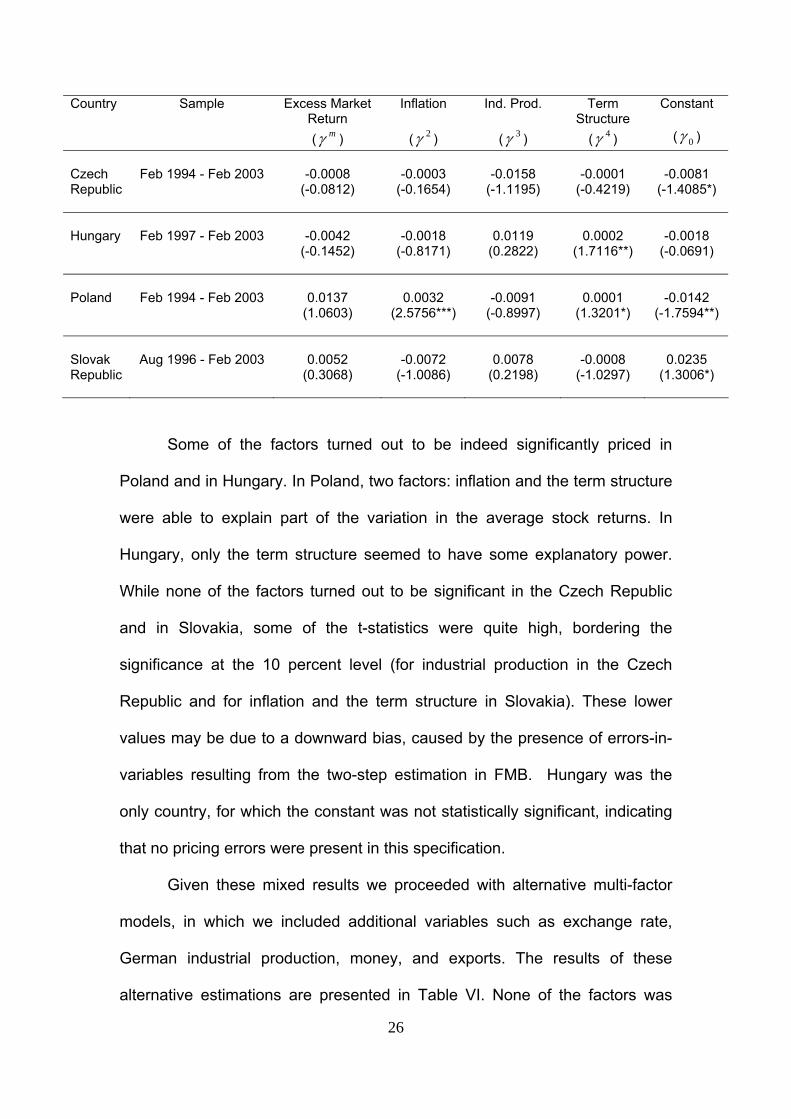
26

Some of the factors turned out to be indeed significantly priced in

Poland and in Hungary. In Poland, two factors: inflation and the term structure

were able to explain part of the variation in the average stock returns. In

Hungary, only the term structure seemed to have some explanatory power.

While none of the factors turned out to be significant in the Czech Republic

and in Slovakia, some of the t-statistics were quite high, bordering the

significance at the 10 percent level (for industrial production in the Czech

Republic and for inflation and the term structure in Slovakia). These lower

values may be due to a downward bias, caused by the presence of errors-in-

variables resulting from the two-step estimation in FMB. Hungary was the

only country, for which the constant was not statistically significant, indicating

that no pricing errors were present in this specification.

Given these mixed results we proceeded with alternative multi-factor

models, in which we included additional variables such as exchange rate,

German industrial production, money, and exports. The results of these

alternative estimations are presented in Table VI. None of the factors was

Country Sample Excess Market Return (γ m )

Inflation

(γ 2 )

Ind. Prod.

(γ 3 )

Term Structure

(γ 4 )

Constant

(γ 0 )

Czech Republic

Feb 1994 - Feb 2003

-0.0008

(-0.0812)

-0.0003

(-0.1654)

-0.0158

(-1.1195)

-0.0001

(-0.4219)

-0.0081

(-1.4085*)

Hungary

Feb 1997 - Feb 2003

-0.0042

(-0.1452)

-0.0018

(-0.8171)

0.0119

(0.2822)

0.0002

(1.7116**)

-0.0018

(-0.0691)

Poland

Feb 1994 - Feb 2003

0.0137

(1.0603)

0.0032

(2.5756***)

-0.0091

(-0.8997)

0.0001

(1.3201*)

-0.0142

(-1.7594**)

Slovak Republic

Aug 1996 - Feb 2003

0.0052

(0.3068)

-0.0072

(-1.0086)

0.0078

(0.2198)

-0.0008

(-1.0297)

0.0235

(1.3006*)

27

significant in the model for the Czech Republic, indicating that these

commonly used macroeconomic factors were not able to explain the variation

in average stock returns in this country. Given these results we decided to

proceed with the basic factor model for the Czech Republic. For Hungary, the

term structure was statistically significant in al model specifications, indicating

that this factor had some explanatory power in this market. By adding

additional factors we are also able to reduce the significance of constant

terms, thus reducing the pricing errors in these models. Having confirmed the

importance of term structure for the Hungarian market even when other

factors are included, we decided to continue with the basic factor model. In

case of Poland, as before, the term structure and inflation were significantly

priced. When money was included in a model, the slope coefficient on inflation

turned insignificant, as money gained explanatory power. By adding additional

factors, we were able to reduce the significance of constant terms. Given the

trade-off between inflation and money, we decided to proceed with the basic

factor model and include inflation rather than money in case of the Polish

market. In the Slovak market, exchange rate and the German industrial

production were both significant when included together with the four factors

encompassing the basic factor model.

28

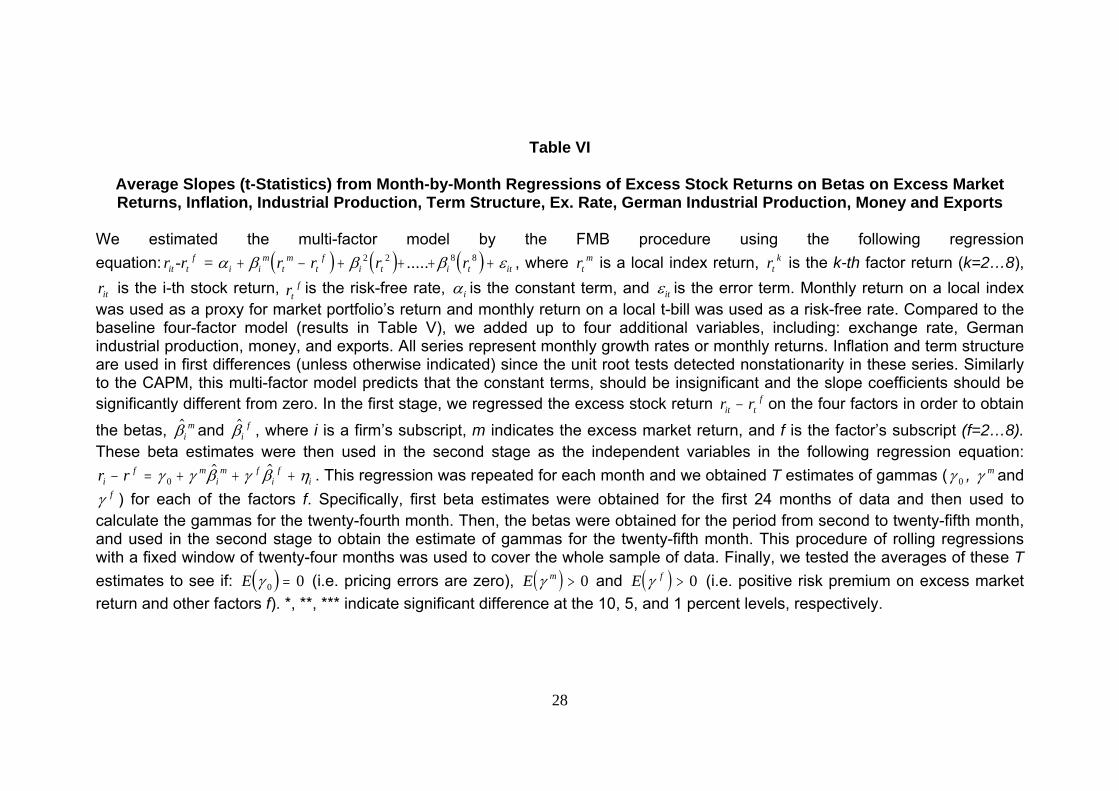
Table VI

Average Slopes (t-Statistics) from Month-by-Month Regressions of Excess Stock Returns on Betas on Excess Market Returns, Inflation, Industrial Production, Term Structure, Ex. Rate, German Industrial Production, Money and Exports

We estimated the multi-factor model by the FMB procedure using the following regression equation: ( ) ( ) ( )r -r = r r r rit t

fi i

mtm

tf

i t i t itα β β β ε+ − + + + +2 2 8 8..... , where rtm

is a local index return, rtk is the k-th factor return (k=2…8),

rit is the i-th stock return, rtf is the risk-free rate, αi is the constant term, and εit is the error term. Monthly return on a local index

was used as a proxy for market portfolio’s return and monthly return on a local t-bill was used as a risk-free rate. Compared to the baseline four-factor model (results in Table V), we added up to four additional variables, including: exchange rate, German industrial production, money, and exports. All series represent monthly growth rates or monthly returns. Inflation and term structure are used in first differences (unless otherwise indicated) since the unit root tests detected nonstationarity in these series. Similarly to the CAPM, this multi-factor model predicts that the constant terms, should be insignificant and the slope coefficients should be significantly different from zero. In the first stage, we regressed the excess stock return r rit t

f− on the four factors in order to obtain

the betas, $βim and $βi

f , where i is a firm’s subscript, m indicates the excess market return, and f is the factor’s subscript (f=2…8). These beta estimates were then used in the second stage as the independent variables in the following regression equation: r ri

f mim f

if

i− = + + +γ γ β γ β η0$ $ . This regression was repeated for each month and we obtained T estimates of gammas (γ 0 , γ m and

γ f ) for each of the factors f. Specifically, first beta estimates were obtained for the first 24 months of data and then used to calculate the gammas for the twenty-fourth month. Then, the betas were obtained for the period from second to twenty-fifth month, and used in the second stage to obtain the estimate of gammas for the twenty-fifth month. This procedure of rolling regressions with a fixed window of twenty-four months was used to cover the whole sample of data. Finally, we tested the averages of these T estimates to see if: ( )E γ 0 0= (i.e. pricing errors are zero), ( )E mγ > 0 and ( )E fγ > 0 (i.e. positive risk premium on excess market return and other factors f). *, **, *** indicate significant difference at the 10, 5, and 1 percent levels, respectively.

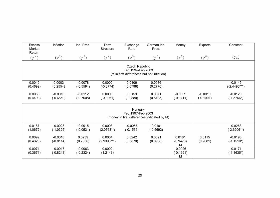
29

Excess Market Return (γ m )

Inflation

(γ 2 )

Ind. Prod.

(γ 3 )

Term Structure

(γ 4 )

Exchange Rate

(γ 5 )

German Ind. Prod.

(γ 6 )

Money

(γ 7 )

Exports

(γ 8 )

Constant

(γ 0 )

Czech Republic

Feb 1994-Feb 2003 (ts in first differences but not inflation)

0.0049

(0.4699) 0.0003

(0.2554) -0.0078

(-0.5594) 0.0000

(-0.3774) 0.0106

(0.6798) 0.0036

(0.2776) -0.0145

(-2.4496***)

0.0053 (0.4499)

-0.0010 (-0.6550)

-0.0112 (-0.7608)

0.0000 (-0.3061)

0.0159 (0.9880)

0.0071 (0.5405)

-0.0009 (-0.1411)

-0.0019 (-0.1001)

-0.0129 (-1.5766*)

Hungary Feb 1997-Feb 2003

(money in first differences indicated by M)

0.0187 (1.0672)

-0.0023 (-1.0325)

-0.0015 (-0.0531)

0.0003 (2.0763**)

-0.0057 (-0.1536)

-0.0101 (-0.5692)

-0.0263 (-2.6206**)

0.0099 (0.4325)

-0.0018 (-0.8114)

0.0239 (0.7536)

0.0004 (2.9398***)

0.0242 (0.6870)

0.0021 (0.0968)

0.0161 (0.9473)

M

0.0115 (0.2681)

-0.0198 (-1.1510*)

0.0074 (0.3671)

-0.0017 (-0.8248)

-0.0063 (-0.2324)

0.0002 (1.2143)

-0.0026 (-0.1691)

M

-0.0171 (-1.1635*)

30

Poland

Feb 1994 - Feb 2003

0.0145 (1.0917)

0.0016 (1.5969*)

-0.0112 (-1.2187)

0.0001 (0.5423)

-0.0009 (-0.0718)

0.0040 (0.4059)

-0.0147 (-1.8957**)

0.0079 (0.6858)

0.0010 (0.7348)

-0.0101 (-1.1014)

0.0001 (1.3070*)

0.0049 (0.3865)

0.0077 (0.7488)

-0.0142 (-1.6670**)

0.0006 (0.0500)

-0.0098 (-1.5903*)

0.0084 (0.6754)

0.0034 (0.9496)

-0.0092 (-0.8465)

0.0002 (1.9772**)

-0.0189 (-1.9010**)

-0.0102 (-1.3336*)

0.0097

(0.8033) -0.0058

(-0.5443) 0.0002

(1.3238*) -0.0170

(-1.6481**)

-0.0115 (-1.5659*)

0.0122

(1.0129) 0.0001

(1.0238) -0.0171

(-1.7302**) -0.0133

(-1.6993**)

Slovakia Aug 1996-Feb 2003

-0.0092

(-0.4443) -0.0051

(-0.5006) -0.0161

(-0.5697) 0.0000

(0.0646) -0.0870

(-2.0689**) -0.0529

(-1.7538*) 0.0183

(0.9716*)

0.0220 (0.6210)

-0.0109 (-1.3398*)

0.0274 (0.5873)

-0.0007 (-0.5537)

-0.0520 (-0.9212)

0.0187 (0.2743)

0.0300 (2.3262***)

0.0669 (0.6648)

-0.0237 (-0.7017)

31

In the next stage, we employed the principal component analysis to

obtain the leading factors, which we then incorporated into a factor model

together with an excess market return. This four-factor model (including three

principal factors/components and an excess market return) was estimated

using FMB. The results of this estimation are presented in Table VII.

Table VII

Average Slopes and t-Statistics (reported in parenthesis) from Month-by-Month Regressions of Excess Stock Returns on Betas on Excess Market

Returns and First Three Principal Factors

We estimated the principal model by the FMB procedure using the following regression equation: ( ) ( ) ( )r -r = r r r rit t

fi i

mtm

tf

i t i t itα β β β ε+ − + + + +2 2 4 4..... , where rt

m is a local index return, rt

k is the k-th principal factor return (k=2…4), rit is the i-th stock return, rt

f is the risk-free rate, αi is the constant term, and εit is the error term. Monthly return on a local index was used as a proxy for market portfolio’s return and monthly return on a local t-bill was used as a risk-free rate. We obtained the principal factors using the principal component analysis. Then, we used the first three as the principal factors in the asset-pricing model. Similarly to the CAPM, this multi-factor model predicts that the constant terms, should be insignificant and the slope coefficients should be significantly different from zero. In the first stage, we regressed the excess stock return r rit t

f− on the excess market return and on the three first principal

factors in order to obtain the betas ( $βim and $βi

f ), where i is a firm’s subscript, m indicates the excess market return, and f is the principal factor’s subscript (f=2…4). These beta estimates were then used in the second stage as the independent variables in the following regression equation: r ri

f mim f

if

i− = + + +γ γ β γ β η0$ $ . This regression was repeated for each month

and we obtained T estimates of γ 0 , γ m and γ f (for each of the factors f). Specifically, first beta estimates were obtained for the first 24 months of data and then used to calculate the gammas (γ 0 , γ m and γ f ) for the twenty-fourth month. Then, the betas were obtained for the period from second to twenty-fifth month, and used in the second stage to obtain the estimate of gammas for the twenty-fifth month. This procedure of rolling regressions with a fixed window of twenty-four months was used to cover the whole sample of data. Finally, we tested the averages of these T estimates to see if: ( )E γ 0 0= (i.e.

pricing errors are zero), ( )E mγ > 0 and ( )E fγ > 0 (i.e. positive risk premium on excess market return and other factors f). *, **, *** indicate significant difference at the 10, 5, and 1 percent levels, respectively.

32

According to the results presented in Table VII, the principal factors

were all significant in case of Poland and one factor was significant in case of

the Slovak Republic. Unlike in previous CAPM and factor models, the local

index was significant in Poland, indicating that it was able to explain some of

the volatility of the stock returns in the Polish market when principal factors

were included. In case of the Slovak Republic, only the third factor was

significant, which captured most of the variation included previously in

exchange rate. None of the principal factors, nor the local market were

significant for the Czech Republic and Hungary.

As argued, the results obtained by using FMB procedure are likely to

be biased due to errors-in-variables problem. In order to verify this hypothesis

we proceeded with alternative GMM estimation, in which all the slope

coefficients (betas and gammas) are estimated simultaneously. We obtained

Country Sample Excess Market Return (γ m )

Pc1

(γ 2 )

Pc2

(γ 3 )

Pc3

(γ 4 )

Constant

(γ 0 )

Czech Republic

Jul 1997 – Feb 2003

0.0021

(0.2175)

-0.1335

(-0.7441)

0.0083

(-0.0433)

0.0526

(0.2177)

-0.0131

(-2.4174***)

Hungary

Jan 1999 – Feb 2003

0.0023

(0.1451)

0.3067

(0.8919)

0.0566

(0.1777)

0.3640

(1.0919)

-0.0107

(-1.1197)

Poland

Feb 1994 - Feb 2003

0.0178

(1.3421*)

0.4562

(1.7947**)

-0.6822

(-1.8727**)

0.5878

(1.7155**)

-0.0166

(-1.7764**)

Slovak Republic

May 1999 – Dec 2002

0.0317

(1.1219)

-0.2340

(-0.2009)

0.1778

(0.1520)

-3.4302

(-1.3085*)

0.0016

(0.1015)

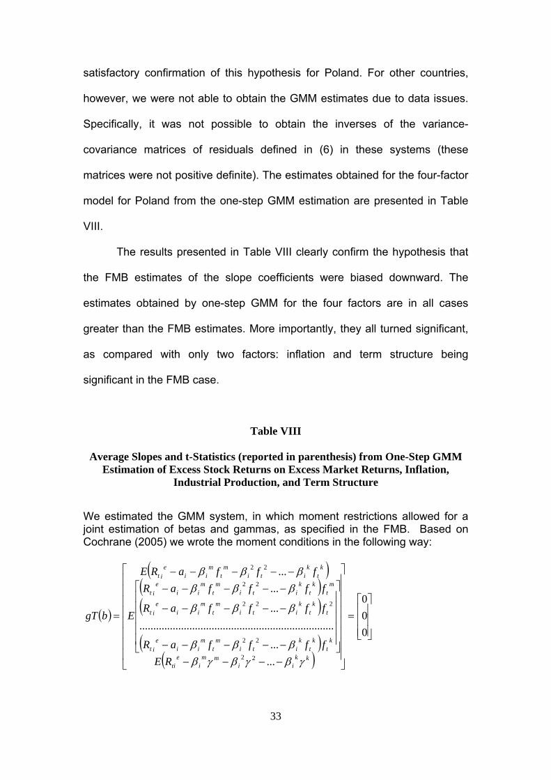
33

satisfactory confirmation of this hypothesis for Poland. For other countries,

however, we were not able to obtain the GMM estimates due to data issues.

Specifically, it was not possible to obtain the inverses of the variance-

covariance matrices of residuals defined in (6) in these systems (these

matrices were not positive definite). The estimates obtained for the four-factor

model for Poland from the one-step GMM estimation are presented in Table

VIII.

The results presented in Table VIII clearly confirm the hypothesis that

the FMB estimates of the slope coefficients were biased downward. The

estimates obtained by one-step GMM for the four factors are in all cases

greater than the FMB estimates. More importantly, they all turned significant,

as compared with only two factors: inflation and term structure being

significant in the FMB case.

Table VIII

Average Slopes and t-Statistics (reported in parenthesis) from One-Step GMM Estimation of Excess Stock Returns on Excess Market Returns, Inflation,

Industrial Production, and Term Structure

We estimated the GMM system, in which moment restrictions allowed for a joint estimation of betas and gammas, as specified in the FMB. Based on Cochrane (2005) we wrote the moment conditions in the following way:

( )

( )( )( )

( )( )

⎥⎥⎥

⎦

⎤

⎢⎢⎢

⎣

⎡=

⎥⎥⎥⎥⎥⎥⎥⎥

⎦

⎤

⎢⎢⎢⎢⎢⎢⎢⎢

⎣

⎡

−−−−

⎥⎥⎥⎥⎥

⎦

⎤

⎢⎢⎢⎢⎢

⎣

⎡

−−−−−

−−−−−

−−−−−−−−−−

=000

......

.........................................................................

......

22

22

222

22

22

kkii

mmi

eti

kt

kt

kiti

mt

mii

eit

tk

tk

itim

tm

iie

it

mt

kt

kiti

mt

mii

eit

kt

kiti

mt

mii

eit

REffffaR

ffffaR

ffffaR

E

fffaRE

bgT

γβγβγββββ

βββ

ββββββ

34

where eitR is the i-th stock excess return (i-th stock return minus risk-free

rate), mtf is a local index excess return (local index return minus risk-free

rate), ktf is the k-th factor return (k=2…4).

In this system there are N(1+K+1) moment conditions since for each asset N we have one moment condition for the constant, K moment conditions for K factors and one moment condition that allows to estimate the lambdas (asset-pricing model condition). We estimated this system by GMM, in which the optimal weighting matrix was obtained in an iterative process by sequential updating of the coefficients. To test the overall model we calculated the J-statistic in the following way: ( ) ( )[ ]bgSbgTJT TT

ˆˆ'ˆ** 1−= , where ( )bgTˆ are the

moment conditions evaluated at estimated values of coefficients β and γ , whereas 1ˆ −S is the inverse of optimal weighting matrix (variance-covariance matrix). This statistic follows approximately 2χ distribution with degrees of freedom equal to number of moment conditions minus the number of parameters. In our case J-statistic was equal to 17.4, whereas 2χ critical value at 95 percent level of significance with 39 degrees of freedom was 18.5. Since J-statistic was less than the appropriate critical value we could not reject the model. *, **, *** indicate significant difference at the 10, 5, and 1 percent levels, respectively.

5. Summary

Emerging markets returns have been quite extensively studied in the

last decade. However, there is still no consensus in the literature as to which

model should be used to explain the returns in these markets and to estimate

the cost of capital. Cost of capital is important information that is needed to

evaluate the investment opportunities, as well as to assess the performance

of managed portfolios. In the developed markets, the CAPM is most often

used to estimate the cost of capital, even though its empirical record is quite

Excess Market Return (γ m )

Inflation

(γ 2 )

Ind. Prod.

(γ 3 )

Term Structure

(γ 4 )

-0.0935 (-2.3566**)

-0.0073

(-1.9595*)

-0.0400

(-1.8555*)

-0.0016

(-2.3029**)

35

poor. Factor models have been developed to overcome some of the CAPM’s

shortcomings, namely the inability of the excess market return alone to

explain the variance of the average stock returns. Factor models extend the

CAPM by adding additional factors to the excess market return in order to

improve the predictive power of the model.

In this paper we tested various asset-pricing models and evaluated

their relative performance in explaining the average stock returns in the

Visegrad countries. These models, as argued, can be used to estimate the

cost of capital, which is then used to evaluate investment opportunities. There

is no consensus in the literature as to which model should be used for this

purpose in the emerging markets. We began by formally estimating the CAPM

by the FMB procedure using the data from the Visegrad markets to see how it

performs. While we were not able to reject the null hypothesis that the CAPM

holds (i.e. constant terms are not significantly different from zero) for Hungary

and Slovakia, we were also not able to reject the null hypothesis that the

coefficients on the factor loading (betas of the excess market return) were

statistically insignificant. In contrast, we could reject the CAPM for the Czech

and Polish markets. Having confirmed the low power of the CAPM in

explaining the variance of the average stock returns we then proceeded to

estimate a factor model. Due to a limited number of stocks traded in the

Visegrad markets we were not able to construct the FF factors. Another

alternative is to use so-called ‘macroeconomic factor models’, in which the

observable economic time series like inflation or interest rates are used as

measures of pervasive or common factors in asset returns. We employed a

macroeconomic factor model based on the factors used by CRR (1986). In

our model we included the following four factors: excess market return,

industrial production, inflation, and excess term structure. We estimated this

four-

factor model using the FMB procedure. This model had some explanatory

power in Poland and in Hungary since some of the slope coefficients were

significant, indicating that the factors were priced. Moreover, in Hungary, the

coefficient on the constant term was not significant; hence there were no

36

pricing errors present in this specification. The coefficients on the constant

terms were, however, significant in the Czech Republic, Poland and in the

Slovak Republic, indicating that some pricing errors were present. Using

alternative macroeconomic variables, as factors largely did not improve the

results10. Given these mixed results, we decided to proceed with the principal

component analysis in order to extract the key factors that explain the

variability of stock returns in these countries. The principal factor model had

some explanatory power in case of Poland and the Slovak Republic. Unlike in

previous CAPM and factor models, the local index was significant in Poland,

indicating that it was able to explain some of the volatility of the stock returns

in the Polish market when principal factors were included. In case of the

Slovak Republic, the slope coefficient on the third factor was significant,

indicating that this factor was priced. The principal factors did not add an

explanatory power in the Czech Republic and Hungary. Based on these

results we concluded that macroeconomic factor model, rather than the capital

asset pricing or the principal factor models, is suitable for estimating the cost

of capital in Visegrad countries. Our conclusion is supported by the results

obtained for Poland when using the one-step GMM estimation method. These

alternative estimates, free of errors-in-variables problem, resulted in all the

factors turning significant, confirming that the FMB estimates were biased

downward. Even though due to empirical problems we were not able to obtain

similar alternative estimates for other Visegrad countries we can expect that

the estimates obtained by the FMB most likely undermine the significance of

macroeconomic factors in explaining the average stock returns.

10 With the exception of Slovakia, for which the exchange rate and the German industrial production were significantly priced in contrast with the factors included in the baseline four-factor model, which were all insignificant.

37

6. References Bartholdy, J. and P. Peare, 2003, Unbiased Estimation of Expected Return Using CAPM, International Review of Financial Analysis, No12, 69–81. Bekaert, G., and C. Harvey, 1995, Time-Varying World Market Integration, Journal of Finance, 50, 403-444. Bekaert, G. and C. Harvey, 2000, Foreign Speculators and Emerging Equity Markets, he Journal of Finance, Vol. 55, No. 2, 565-613 Black, F., 1972, Capital Market Equilibrium with Restricted Borrowing, Journal of Business, 45, 444-455. Black F., M. Jensen and M. Scholes, 1972, The Capital-Asset Pricing Model: Some empirical tests, in Jensen: Studies in the Theory of Capital Markets. Brealey, R. A. and S. C. Myers, 1988, Principles of Corporate Finance, McGraw-Hill Book Company. Chen, N., R. Roll, and S.A. Ross, 1986, Economic Forces and the Stock Market, Journal of Business 59, 383-403. Cochrane, J. H., 2005, Asset Pricing, Princeton University Press, pp. 241-242. Cuthbertson, K. and D. Nitzsche, 2004, Quantitative Financial Economics : Stocks, Bonds and Foreign Exchange, John Wiley & Sons Ltd. Erb, C., C. Harvey, and T. Viskanta, 1995, Country Risk and Global Equity Selection, Journal of Portfolio Management, Winter, 74-83. Erb, C., C. Harvey, and T. Viskanta, 1996, Expected Returns and Volatility in 135 Countries, Journal of Portfolio Management, Spring, 46-58. Fama, E.F. and K.R. French, 1993, Common Risk Factors in the Returns on Stocks and Bonds, Journal of Financial Economics, 33, 3-56. Fama, E.F. and K.R. French, 2004, The CAPM: Theory and Evidence, Journal of Economic Perspectives, 18, 25-46. Fama, E.F. and J.D. MacBeth, 1973, Risk, Return, and Equilibrium: Empirical Tests, Journal of Political Economy, 81, 607-636. Graham, J.R. and C. R Harvey, 2001, The Theory and Practice of Corporate Finance: Evidence from the Field, Journal of Financial Economics: 60, 187-243. Harvey, C. R., 1995, Predictable Risk and Returns in Emerging Markets, The Review of Financial Studies, Vol. 8, No. 3, 773-816.

38

De Jong, F. and F. A. de Roon, 2001, Time-Varying Market Integration and Expected Returns in Emerging Markets, CentER Discussion Paper, No 78. Koulafetis, P. and M. Levis, 2002, The Fama-MacBeth Methodology versus the Non-Linear Unrelated Regression and Different Portfolio Formation Criteria, EFMA 2002 London Meetings, http://ssrn.com/abstract=314383 Lakonishok, J. and A. Shapiro, 1986, Systematic Risk, Total Risk, and Size as Determinants of Stock Market Returns, Journal of Banking and Finance, 10, 115-132. Leledakis, G., I. Davidson and G. Karathanassis, 2003, Cross-sectional Estimation of Stock Returns in Small Markets: The Case of the Athens Stock Exchange, Applied Financial Economics, No. 13, 413-426. Lintner, J., 1965, The Valuation of Risky Assets and the Selection of Risky Investments in Stock Portfolios and Capital Budgets, Review of Economics and Statistics 47, 13-37. Low, C. and S. Nayak, 2005, The Non-Relevance of the Elusive Holy Grail of Asset Pricing Tests: the 'True' Market Portfolio Doesn't Really Matter", EFA 2005 Moscow Meetings Paper, http://ssrn.com/abstract=675423 Reinganum, M., 1981, Misspecification of Capital Asset Pricing: Empirical anomalies, Journal of Financial Economics 9, 19-46. Roll R., 1977, A Critique of the Asset Pricing Theory’s Tests, Journal of Financial Economics, No 4, 129-176. Sharpe, W., 1964, Capital Asset Prices: A Theory of Market Equilibrium Under Conditions of Risk, The Journal of Finance, 19, 425-442. Sokalska, M., 2001, What Drives Equity Returns in Central and Eastern Europe, Working Paper, Warsaw School of Economics.

39

Appendix: Description of Data Used in the Principal Component

Analysis All data was downloaded from the IMF’ International Financial Statistics (IFS) Database. The series were downloaded for the quarterly frequency and then transformed into monthly frequency by the constant sum method (the quarterly value is divided by three and for each of the three months in this quarter the same value is repeated). The time series were imported into Eviews and automatically converted into logarithms of the original series if the values were positive. Then, unit root tests were performed and each series was differenced sufficient number of times to achieve stationarity. These series were then used in the principal component analysis. Series name Units

Foreign Assets (Net) Units of National Currency

Domestic Credit Units of National Currency

Claims on General Government (Net) Units of National Currency

Claims on Other Resident Sectors Units of National Currency

Money, Seasonally Adjusted Units of National Currency

Changes in Money Percent Per Annum

Money Units of National Currency

Quasi-Money Units of National Currency

Capital Accounts Units of National Currency

Other Items (Net) Units of National Currency

Monetary Authorities: Other Liabilities Millions of US$

Discount Rate (End of Period) Percent Per Annum

Money Market Rate Percent Per Annum

Treasury Bill Rate Percent Per Annum

Deposit Rate Percent Per Annum

Lending Rate Percent Per Annum

Share Price Index Index Number

Producer Prices: Industry Index Number

Changes in Consumer Prices Percent Per Annum

Wages: Average Earnings Index Number

Industrial Production Index Number

Industrial Employment Index Number

Unemployment Unspecified Unit

Employment Unspecified Unit

Unemployment Rate Percent Per Annum

Exports Millions of US$

Exports, F.O.B. Units of National Currency

Imports Millions of US$

40

Imports, C.I.F. Units of National Currency

Imports, National Currency FOB Units of National Currency

Volume of Exports Index Number

Import Unit Value Index Number

Export Prices Index Number

Import Prices Index Number

Export Prices Index Number

Import Prices Index Number

Deposit Money Banks: Assets Millions of US$

Deposit Money Banks: Liabilities Millions of US$

Deficit (-) or Surplus Units of National Currency

Total Financing Units of National Currency

Revenues Units of National Currency

Total Revenue and Grants Units of National Currency

Grants Units of National Currency

Expenditure Units of National Currency

Expenditure & Lending Minus Repayments Units of National Currency

Lending Minus Repayments Units of National Currency

Domestic Units of National Currency

Foreign Units of National Currency

Total Debt by Residence Units of National Currency

Domestic Units of National Currency

Foreign Units of National Currency

Exports of Goods and Services Units of National Currency

Government Consumption Expenditures Units of National Currency

Gross Fixed Capital Formation Units of National Currency

Changes in Inventories Units of National Currency

Household Consumption Expenditures Including NPISHS Units of National Currency

Imports of Goods and Services Units of National Currency

Gross Domestic Product (GDP) Units of National Currency

GDP Deflator 1995=100 Index Number

GDP Volume (1995=100) Index Number

Official Rate Units of National Currency

Exchange Rate Index 1995=100 Index Number

Nominal Effective Exchange Rate Index Number

Real Effective Exchange Rate Index Number

Actual Holdings in % of Quota Index Number

Total Liabilities % of Quota Index Number

Individual researchers, as well as the on-line and printed versions of the CERGE-EI Working Papers (including their dissemination) were supported from the following institutional grants:

• Center of Advanced Political Economy Research [Centrum pro pokročilá politicko-ekonomická studia], No. LC542, (2005-2009),

• Economic Aspects of EU and EMU Entry [Ekonomické aspekty vstupu do Evropské unie a Evropské měnové unie], No. AVOZ70850503, (2005-2010);

• Economic Impact of European Integration on the Czech Republic [Ekonomické dopady evropské integrace na ČR], No. MSM0021620846, (2005-2011);

Specific research support and/or other grants the researchers/publications benefited from are acknowledged at the beginning of the Paper. (c) Magdalena Morgese Borys, 2007 All rights reserved. No part of this publication may be reproduced, stored in a retrieval system or transmitted in any form or by any means, electronic, mechanical or photocopying, recording, or otherwise without the prior permission of the publisher. Published by Charles University in Prague, Center for Economic Research and Graduate Education (CERGE) and Economics Institute ASCR, v. v. i. (EI) CERGE-EI, Politických vězňů 7, 111 21 Prague 1, tel.: +420 224 005 153, Czech Republic. Printed by CERGE-EI, Prague Subscription: CERGE-EI homepage: http://www.cerge-ei.cz Editors: Directors of CERGE and EI Managing editors: Deputy Directors for Research of CERGE and EI ISSN 1211-3298 ISBN 978-80-7343-122-8 (Univerzita Karlova. Centrum pro ekonomický výzkum a doktorské studium) ISBN 978-80-7344-111-1 (Národohospodářský ústav AV ČR, v. v. i.)