DI

SC

US

SI

ON

P

AP

ER

S

ER

IE

S

Forschungsinstitut zur Zukunft der ArbeitInstitute for the Study of Labor

Testing for IIA with the Hausman-McFadden Test

IZA DP No. 5826

June 2011

Wim Vijverberg

Testing for IIA with the

Hausman-McFadden Test

Wim Vijverberg CUNY Graduate Center

and IZA

Discussion Paper No. 5826 June 2011

IZA

P.O. Box 7240 53072 Bonn

Germany

Phone: +49-228-3894-0 Fax: +49-228-3894-180

E-mail: iza@iza.org

Any opinions expressed here are those of the author(s) and not those of IZA. Research published in this series may include views on policy, but the institute itself takes no institutional policy positions. The Institute for the Study of Labor (IZA) in Bonn is a local and virtual international research center and a place of communication between science, politics and business. IZA is an independent nonprofit organization supported by Deutsche Post Foundation. The center is associated with the University of Bonn and offers a stimulating research environment through its international network, workshops and conferences, data service, project support, research visits and doctoral program. IZA engages in (i) original and internationally competitive research in all fields of labor economics, (ii) development of policy concepts, and (iii) dissemination of research results and concepts to the interested public. IZA Discussion Papers often represent preliminary work and are circulated to encourage discussion. Citation of such a paper should account for its provisional character. A revised version may be available directly from the author.

IZA Discussion Paper No. 5826 June 2011

ABSTRACT

Testing for IIA with the Hausman-McFadden Test* The Independence of Irrelevant Alternatives assumption inherent in multinomial logit models is most frequently tested with a Hausman-McFadden test. As is confirmed by many findings in the literature, this test sometimes produces negative outcomes, in contradiction of its asymptotic χ 2 distribution. This problem is caused by the use of an improper variance matrix and may lead to an invalid statistical inference even when the test value is positive. With a correct specification of the variance, the sampling distribution for small samples is indeed close to a χ 2 distribution. JEL Classification: C12, C35 Keywords: multinomial logit, IIA assumption, Hausman-McFadden test Corresponding author: Wim Vijverberg CUNY Graduate Center 365 5th Avenue New York, NY 10016-4309 USA E-mail: wvijverberg@gc.cuny.edu

* I appreciate the comments and contributions of seminar participants at Hunter College, Rutgers University at Newark, West Virginia University, and Wichita State University and in particular an insightful suggestion by Stratford Douglas.

1 Introduction

Multinomial logit models are valid under the Independence of Irrelevant Alternatives (IIA)

assumption that states that characteristics of one particular choice alternative do not impact

the relative probabilities of choosing other alternatives. For example, if IIA is valid, how I

choose between watching a movie or attending a football game is independent of whoever

is giving a concert that day. Violation of the IIA assumption complicates the choice model.

Therefore, much is gained when the IIA assumption is validated.

A number of tests of the IIA exist. One test was devised by Hausman and McFadden

(1984) as a variation of the Hausman (1978) test. It relies on the insight that (i) under

IIA, the parameters of the choice among a subset of alternatives may be estimated with

a multinomial logit model on just this subset or on the full set, though the former is less

efficient than the latter, and (ii) if IIA is not true, the parameter estimates of the full set are

inconsistent, whereas those of the subset are consistent provided that the subset is properly

selected. This test is implemented simply by two (multinomial) logit estimations and an

evaluation of the difference in the parameter estimates. Other tests include one designed

by Small and Hsiao (1985), which builds on McFadden, Train, and Tye (1977); another test

proposed by Hausman and McFadden (1984) based on an estimation of the nested logit

model; tests based on regression-based statistics by McFadden (1987) and Small (1994); a

nonparametric test by Zheng (2008); and a test by Weesie (1999) that will be discussed

below.

For the purpose of this paper, let us denote the Hausman-McFadden testing strategy as

the HM test and the popular implementation of this test as the H test, to be contrasted with

the H test that will be defined later on. The H test is by far the most frequently used test,

undoubtedly in no small part due to its simplicity. To illustrate, over the period from 1984

to February 2010, there were 388 studies published in the scholarly literature that cited the

1

Hausman and McFadden (1984) paper, 276 of which applied the H test for a total of 433

test results (Table 1).1 In fact, the use of this test is accelerating: as Table 1 shows, the test

was applied in as many studies in the last five years as in the first 20 years. Furthermore, the

test was included in comparative simulation studies by Fry and Harris (1996, 1998), Cheng

and Long (2007), and Zheng (2008); Small and Hsiao (1985) and Zhang and Hoffman (1993)

offer a numerical comparison as well.

One inconvenient finding about the H test is that, even though its asymptotic distribution

is χ2 and its outcomes should be therefore strictly positive, in applied situations the test

statistic sometimes yields negative outcomes. That negative values may occur has long been

known, starting with Hausman and McFadden (1984, p.1226) who suggest that a negative

outcome of the H test may still be taken as support for the Null hypothesis. The literature

clearly subscribes to this view: as Table 1 indicates, most studies do not reject IIA when H

is negative, and the Monte Carlo study of Cheng and Long (2007) continues this practice.

However, negative values occur frequently: in the literature described in Table 1, 16.2 percent

of the reported test values are negative, and one may suspect that the test statistic may well

be negative among some of the 32 percent of the cases where authors merely make mention

of the test without reporting its actual value.

The frequent occurrence of these negative values has unappreciated consequences. In

this paper, I contend that H is a test statistic with poor properties that, compounded by

errors in inference that are due to its common implementation, has put a significant body

of empirical research at risk. However, a better version of the HM test is readily available.

Through simulations as well as analytically derived small-sample distributions, I show

1These statistics are drawn from the Web of Science exclusively. Apart from the 276 studies that citedHausman and McFadden (1984) as a reference for the test that was implemented, 47 studies used its contri-bution as a building block in their own pursuits; 61 made reference without a clear indication how it addedvalue; and 4 listed the paper in the bibliography section but made no reference to it in the study itself.By comparison, McFadden, Train, and Tye (1977) was cited 76 times for all purposes combined; Small andHsiao (1985) was cited 73 times; McFadden (1987) was cited 36 times; Small (1994) was cited 13 times; andZheng (2008) has not been cited yet.

2

that the asymptotic χ2 distribution offers a poor approximation to the small-sample dis-

tribution of H for samples with 1000, 7500 or even 100,000 observations. The reason is

that the H test inserts a variance estimator of the parameter difference that is conceptually

inconsistent with the research question. This has two consequences. First, this (estimated)

variance matrix may become indefinite, according to our simulations not just occasionally

but actually very frequently even in very large samples. When this happens, large differences

between estimates of full and restricted models may equally well result in large positive or

large negative values of the H test, or small values for that matter. The fact that the variance

matrix may be indefinite also means that the test statistic must not be accepted as “valid”

whenever the variance happens to be positive definite. The inserted variance is part and

parcel of H; therefore, H has a distribution different from χ2. This leads us to the second

consequence: H is a pivotal test statistic only asymptotically. In small samples, its sampling

distribution depends on the sample at hand in two ways: (i) it uses parameter estimates

of both the full and the restricted model, and (ii) it is conditional on the sample’s choice

outcomes. With much effort, an unconditional distribution under IIA may be derived, but

the (estimated) sampling distribution remains sample-dependent and, as simulations show,

is not robust.

The conceptually correct formulation of the HM test will be referred to as the H test. Its

small-sample distribution does not deviate greatly from its asymptotic χ2 sampling distri-

bution: H is remarkably robust against small-sample deviations from non-normality in the

parameter estimates. This formulation was mentioned almost parenthetically by Hausman

and McFadden (1984), but it has not been taken seriously in the literature and is rarely

implemented in practice (Table 1).2 Overall, H performs significantly better than H.

2Hausman and McFadden (1984, p.1226) argued on the basis of work with H (at a time where computingpower limited Monte Carlo research relative to today’s standards) that negative values of H may be takenas support for the Null hypothesis. For some data structures, H actually proves to have little power, whichcould explain this recommendation.

3

HM tests must flag samples for which differences in restricted and unrestricted parameter

estimates are large. Across many simulations where IIA was violated, for those samples that

were flagged by H at a 5 percent significance level, the size-corrected probability that H was

significant was only about 11 percent in small (n = 1000) samples and 21 percent in larger

(n = 7500) samples—and H actually fell in its 5-percent left tail about 6 percent of the time.

Most of the time, H was insignificant. Combined with the fact that H is typically judged by

its asymptotic χ2 distribution and thus not evaluated properly, this strongly suggests that

many among the 276 studies summarized in Table 1 may have made erroneous inferences:

rejections of IIA may have been invalid, and acceptances of IIA may have been incorrect.

As mentioned, the inserted variance estimate is the cause of the troubles with the H test.

Weesie (1999) developed a general sandwich variance estimator that may be applied to HM

tests for IIA as well. It ensures that the estimated variance is positive definite, yielding a

formulation of the HM test that will be referred to as Hs.3 As this paper shows, in small

samples Hs is exceedingly conservative and, even after size correction, is less powerful than

H.

In the following, Section 2 discusses the differences between the two versions of the

Hausman-McFadden test and derives their analytical small-sample distributions, subject to

certain restrictions. Section 3 examines these restrictions and the H and H tests in a Monte

Carlo context. Section 4 compares the analytical small-sample densities with their simulated

counterparts. Section 5 describes Weesie’s Hs test and the Monte Carlo evidence about it.

Section 6 applies the three versions of the HM test, and Section 7 concludes.

3However, the literature has largely ignored (or been ignorant of) this test: over the period 2000-2010,only four studies that perform tests for IIA apply the Hs test that is based on Weesie (1999).

4

2 The HM test

This section reexamines the common implementation of the Hausman-McFadden test for

IIA. It is shown to rely on a shortcut that leads to a specification of a variance estimator

that contradicts the principle of comparison between the two multinomial logit models that

are being compared by the test. However, the specification of the test can be improved

upon with a simple modification. This section also develops tools to examine small-sample

properties of the test statistics.

2.1 Two specifications of the HM test

Let sample Sr = 1, ..., n consist of n individuals who each choose from J alternatives in

the choice set C = 1, ..., J. Across the different samples (r = 1, 2, . . . , R), the choice set

remains the same. The index r is suppressed in the notation until the appropriate time.

The utility derived from alternative j is given by

Uji = Xiβj + εji, j ∈ C, i ∈ Sr (1)

where Xiβj represents the systematic component of utility and εji the stochastic component.

Alternative j is chosen if Uji > max (Uki, k 6= j). Accordingly, define yji = 1 if j is chosen

and = 0 if not. Under the Null hypothesis of IIA, εji is distributed Gumbel. Then, the

log-likelihood function may be written as

lnLC =n∑i=1

∑j∈C

yjiXiβj −n∑i=1

ln

(∑k∈C

eXiβj

)(2)

Let βJ = 0 for standardization, and define β =(β′1, · · · , β′J−1

)′. Its true value is denoted as

β0. Let β maximize lnLC . Then, asymptotically, β is distributed under H0 as N(β0,Σ0C)

5

with

Σ0C =

(−E0

[hC(β0)

])−1 ≡ ΣC(β0) (3)

where block j, k of the hessian is given by

[hC(β0)

]jk

=∂2 lnLC(β0)

∂βj∂β′k= −

n∑i=1

p0ji(I(j = k)− p0ki

)XiX

′i (4)

in which p0ji = eXiβ0j /∑

k∈C eXiβ

0k and I is the familiar indicator function. Equation (4)

does not contain any random term, and so the expectation of it in equation (3) is the same

expression. In estimation, β is substituted for β0. We label the variance estimator therefore

as ΣC = ΣC(β).

For this same sample, let us test for IIA by removing some of the alternatives from the

choice set. The remaining choice set is denoted as D, which must be specified a priori, and

let D† = C \D be D’s complement. Without loss of generality it is assumed that D contains

alternative J and that it is once again the basis for standardization. Let yDi be the indicator

that individual i selects any j ∈ D: yDi =∑

j∈D yji. Define βD as the vector that stacks βj

for j ∈ D \ J, and extract β0D similarly from β0. Then the log-likelihood function for

this estimation problem is:

lnLD =n∑i=1

yDi

(∑j∈D

yjiXiβj − ln

(∑k∈D

eXiβj

))(5)

Let βD be the estimator that maximizes lnLD.

In the common formulation of this estimation problem, the summation over i is made

only over the subsample Sr(D) of members of Sr who select an alternative j ∈ D, and yDi

6

vanishes as it always equals 1. Denote this formulation as ln LDr:

ln LDr =∑

i∈Sr(D)

∑j∈D

yjiXiβj −∑

i∈Sr(D)

ln

(∑k∈D

eXiβj

)(6)

In other words, this becomes a regular MNL model estimated over a smaller sample and a

smaller choice set. Taken as such, this leads to the conclusion that the asymptotic variance

of βD is given by

Σ0Dr =

(−E0

[h0Dr(β

0D)])−1 ≡ ΣDr(β

0D) (7)

where for j, k ∈ D:

[h0Dr(β

0D)]jk

=∂2 ln LD(β0

D)

∂βj∂β′k= −

∑i∈Sr(D)

q0ji(I(j = k)− q0ki

)XiX

′i (8)

with q0ji = eXiβ0j /∑

k∈D eXiβ

0k = p0ji/p

0Di, where p0Di =

∑k∈D p

0ki. As before, in estimation, βD

is substituted for β0D, and we label the variance estimator therefore as ˘ΣDr = ΣDr(βD).

However, the likelihood function given in equation (5) yields a different expression for

the variance of βD:

Σ0D =

(−E0

[h0D(β0

D)])−1 ≡ ΣD(β0) (9)

where the expected value of block j, k of the hessian equals

ED

[[h0D(β0

D)]jk

]= E0

[∂2 lnLD(β0

D)

∂βj∂β′k

]= E

[−

n∑i=1

yDiq0ji

(I(j = k)− q0ki

)XiX

′i

]

= −n∑i=1

p0Diq0ji

(I(j = k)− q0ki

)XiX

′i

= −n∑i=1

p0ji(I(j = k)− q0ki

)XiX

′i (10)

Note that p0ji, even for j ∈ D, is a function of the entire β0 vector. Thus, Σ0D depends on

7

β0. Accordingly, to estimate Σ0D, we insert β: ΣD = ΣD(β).

What is the difference between Σ0D and Σ0

Dr? The answer lies in the recognition of εji

for all j = 1, . . . , J and all i = 1, . . . , n as the source of randomness. Σ0Dr describes the

variation in βD that results from confronting members of the subsample Sr(D) with different

realization of the world, by assigning them different draws of εji for j ∈ D and restricting

their choice to choice set D only. The membership of this subsample does not change; only

what they choose from D is changing. On the other hand, Σ0D describes the variation in βD

that results from assigning different draws of εji for all j ∈ C to the entire sample Sr, not

just for j ∈ D. Some members of Sr(D) will no longer choose j ∈ D, and some of Sr(D†) will

now choose j ∈ D. Given that sample Sr rather than the subsample Sr(D) is the basis of the

test for IIA, this second characterization of the randomness in βD is conceptually preferable

to the first.

It could be argued that ˘ΣDr and ΣD are merely two alternative estimators of Σ0D. Indeed,

they are, with two differences between them. First, they rely on different estimators of β,

namely βD and β, respectively. Second, rewrite equation (8) as

[h0Dr]jk

= −∑

i∈Sr(D)

q0ji(I(j = k)− q0ki

)XiX

′i

= −n∑i=1

yDiq0ji

(I(j = k)− q0ki

)XiX

′i =

[h0D]jk

(11)

This highlights the fact that the expectation in equation (7) is conditional on selection of

D (i.e., on yD) by members of Sr. Thus, it is more accurate to write Σ0Dr = ΣD(β0

D, yDr).

Then, compare the second line of equation (10) with equation (11): to estimate Σ0D, yDi is

substituted for pDi. Asymptotically, this does not matter since ˘Σ0D converges to Σ0

D as n

goes to ∞ (Appendix A). But in a small sample yDi is a poor substitute for pDi.4

4Of course, if the objective is to study the choice of alternatives from choice set D and samples are drawnaccordingly, the estimator ΣD(βD) is appropriate, just as ΣC(β) is for what is considered to be the “full”model in this paper.

8

This brings us to formulations of the HM test statistic. Let βD be the estimator of βD that

is extracted from β of the full MNL model; its variance Σ0C,DD consists of the corresponding

submatrix of Σ0C . Define δD = βD − βD. If IIA applies, the mean of δD equals 0, and its

asymptotic variance equals

Ω0D = Σ0

D − Σ0C,DD ≡ Ω(β0) (12)

In principle, the HM test statistic is then given by H = δ′DΩ0D−1δD. H is actually infeasible

since Ω0D is unknown, but it serves a purpose in the Monte Carlo study. In line with the

previous discussion, Ω0D may be estimated with ΩD = Ω(β) or with ˘ΩDr = ΣD(βD, yDr) −

ΣC,DD(β). Ω0D and ΩD are positive definite (see Appendix B), but nothing can be said

about ˘ΩDr. On the basis of these, the test statistics are denoted as H = δ′DΩ−1D δD and

H = δ′D˘Ω−1DrδD. H is the common formulation of the HM test that is used in nearly every

study that tests for IIA. H uses a conceptually preferred estimator of Ω0D.

Hausman and McFadden (1984) mention H almost parenthetically and then only as a

fix in case ˘ΩDr is indefinite and as a way to motivate that a negative outcome of H may

well indicate non-rejection of the Null hypothesis. The Monte Carlo analysis in Section 3

will shed light on the validity of this assessment. In particular, H is negative so often that

it would not be right to discard such outcomes and proceed to another test. Moreover, the

differences between ˘ΣDr and ΣD have the potential to cause a significant distortion in H

relative to H, which the literature has not yet recognized to be problematic.5

At a few points in the analysis below, we will compare H and H with He = δ′D(ΩeD)−1δD,

where ΩeD is the empirical covariance matrix of simulated δD values generated under the

null hypothesis, i.e., a simulation-based estimator of ΩD that is independent of any model

5Instead of replacing ˘ΣDr with ΣD, we could replace ΣC by a variance of β computed under conditionalsampling that assigns draws of εji for all i = 1, . . . , n such that the composition of subsamples Sr(D) and

Sr(D†) stays the same. Under such conditional sampling, β would actually be biased and inconsistent(Appendix C). Thus a HM test statistic that is derived from a conditional sampling approach would beflawed from the start.

9

structure. Because it is computation-intensive, it is not at the center of our interest, but

it does offer a yardstick to evaluate outliers of the HM statistics without the structure

that accompanies ΩD or ˘ΩDr. Moreover, in Section 5, we will examine the consequences of

estimating Ω0D with the sandwich estimator proposed by Weesie (1999).

2.2 Small-sample distribution of the HM tests

As ΩDr is not guaranteed to be positive definite—and indeed frequently is indefinite—, the

small-sample distribution may well deviate substantially from the asymptotic χ2 distribution.

Let us therefore develop tools to analyze the small-sample properties of the distribution of

the HM tests.

It is beneficial to reorder β such that β =(β′D† , β

′D

)′, such that the parameters associated

with D appear at the bottom; note that βJ = 0 because of standardization. Write H in

terms of(β′, β′D

)′:

H =

β

βD

′

R′D

(RDVDR

′D

)−1R

β

βD

(13)

where VD is the estimated variance of(β′, β′D

)′:

VD =

ΣC

ΣC,DD†

ΣC,DD

ΣC,D†D ΣC,DD ΣD

. (14)

and where R = (0 ID − ID), such that ID is an identity matrix conformable with βD and 0

is a matrix of zeroes. Thus(RDVDR

′D

)= ΩD. H may be rewritten in the same way, using

˘VDr instead of VD where ˘VDr is similar to equation (14) with ˘ΣDr substituted for ΣD.

Since ˘VD 6= VD ≈ Var

((β′, β′D

)′), we may call on the procedure developed by Imhof

(1961) to evaluate the distribution under the null hypothesis. A precise description of this

10

procedure is useful for an understanding of the small-sample behavior of the HM test statis-

tics. In general terms, let an m-dimentional vector δ be distributed N(δ,Ω). Consider the

quadratic form H = δ′Aδ. Use the Cholesky decomposition to define P such that Ω−1 = PP ′

and P ′ΩP = I. Then, rewrite H:

H = δ′Aδ = δ′PP−1A(P ′)−1P ′δ = δ′PEΘE ′P ′δ = η′Θη =m∑j=1

θj η2j =

m∑j=1

θjχ2(1, µ2

j) (15)

where the third equality uses the singular value decomposition such that E and Θ = diag(θj)

are the matrices of eigenvectors and eigenvalues of P−1A(P ′)−1, and where η = C ′P ′δ is

distributed N(µ, Im) with µ = E ′P ′δ.6 Provided that all eigenvalues are unique, H is

distributed as a weighted sum of noncentral χ2 random variables with degrees of freedom

equal to 1 and noncentrality parameter µ2j .

7

In the case of H under the null hypothesis of IIA, we have δ = 0, A = ΩD and Ω = Ω0D.

Thus, µj = 0 for all j. Since Ω0D is estimated by ΩD, we have P−1A(P ′)−1 = I, Θ = I,

and the estimated sampling distribution of H is χ2. In the case of H, δ = 0, A = ˘ΩDr and

Ω = Ω0D. Since ˘ΩDr 6= ΩD, H is distributed as a weighted sum of χ2(1) variates. Moreover,

whenever ˘ΩDr is an indefinite matrix, some of the eigenvalues are negative. In such a case,

the estimated distribution of H has a left tail stretching to −∞. Unusually large values of δ

may therefore result in outcomes of H in the right as well as the the left tail: the rejection

range should be not merely the right tail. We return to this issue at the end of Section 3.2

when the quantitative importance of the left tail has become clearer.

Next, let us consider the sampling distribution under an alternative hypothesis. Many

conditions could lead to a violation of IIA, but we employ the nested logit model as the

6By implication, Θ is also the matrix of eigenvalues of AΩ.7In case eigenvalues appear with multiplicity greater than 1, the associated η2j are combined into a single

χ2 with degrees of freedom equal to the multiplicity of that eigenvalue and a noncentrality parameter equalto the sum of the associated µ2

j . In our analysis of H (and of H under non-IIA), eigenvalues happen to bedistinct.

11

model that is valid under the alternative hypothesis.8 According to the nested logit model,

the probability that choice j is selected equals

P (yi = j|Xi) = pji =eXiβj

Fifor j ∈ D†

=eλIi

Fi

eXiβj/λ

Eifor j ∈ D (16)

where Ii = ln∑

j∈D eXiβj/λ, Fi =

∑j∈D† eXiβj + eλIi , and Ei = eIi .

The likelihood functions that are maximized are given by equations (2) and (5). Let

the gradients be given by gC(β) and gD(βD), respectively. Approximate gC at βa, which is

chosen such that E[gC(βa)] = 0 and thus equals the vector to which β converges as n→∞:

0 = gC(β) ≈ gC(βa) + hC(βa)(β − βa

)(17)

Approximate gD at βbD, which is chosen such that E[gD(βbD)] = 0:

0 = gD(βD) ≈ gD(βbD) + hD(βbD)(βD − βaD

). (18)

In view of equation (16), we have βbD = β0D/λ

0 if the test specifies D correctly. The following

results are straightforwardly derived:

E[gC(βa)gC(βa)′] = −h0C (19)

E[gD(βbD)gD(βbD)′] = −hD(βbD) (20)

8For example, violations of IIA may be related to arbitrary correlations among the εj , to nonlinearityamong linearly-included explanatory variables or to omitted explanatory variables; see Train (2009) for agood discussion. The nested logit model asserts that the only form of misspecification in the MNL model isthe failure to account for a specific type of correlation among the εj .

12

E[gC(βa)gD(βbD)′] =

0

−hD(βbD)

(21)

where h0C is the same as the right hand side of equation (4) with probabilities p0ji evaluated

through equation (16) at (β0, λ0). Thus,

VD =

hC(βa)−1 0

0 hD(βbD)−1

−h0C0

−hD(βbD)

0 −hD(βbD) −hD(βbD)

hC(βa)−1 0

0 hD(βbD)−1

(22)

Since h0C 6= hC(βa), VD no longer simplifies neatly, and in its estimated form, RVDR′ is

no longer equal to ΩD. The sampling distribution of both H and H are weighted sums of

non-central χ2(1, µ2j) distributions, with µ derived from δ = βbD − βaD.

These tools are predicated on the assumption that β and βD are normally distributed with

means equal to βa and βbD respectively and variances that are stated above. In the following

section, we first report on Monte Carlo simulations that put a face on the analytical results

and in the process examine the validity of this normality assumption in an ideal Monte Carlo

world, and then evaluate the analytical sampling densities under the null and alternative

hypotheses.

3 Monte Carlo evidence

3.1 Design

To examine the performance of the different versions of the Hausman-McFadden statistic,

we employ three sets of data for both J = 3 and J = 4 in small and large sample versions.

The first dataset is synthetic and is typical among Monte Carlo studies: it contains 1000

observations in the small sample version and 7500 observations in the large sample version;

13

the two explanatory variables are draws of standard normal variables with a correlation of

about 0.48; and values for β are chosen such that one alternative is relatively dominant (Table

2). The second dataset is synthetic as well and is inspired by Cheng and Long (2007): with

either 1000 or 7500 observations, its first variable is a uniform draw; its second is a normal

draw added to the first variable; its third is a χ2(1) draw added to the first variable; and the

weights in this construction are chosen such that the correlation between the first and second

variable is high (0.75) and moderate between the third and the first two (about 0.30). Thus,

the second dataset is characterized by both multicollinearity and skewness. Again, values

for β are chosen such that one alternative is relatively dominant. The third dataset derives

from an analysis of employment activities among men in Cote d’Ivoire in urban areas other

than Abidjan (Vijverberg, 1993). The explanatory variables consist of years of schooling and

of apprenticeship, age, age squared, and four dummy variables (marital status, citizenship,

and two time dummies). For β, we use parameters that are estimated from a MNL model

of the actual employment choice in this sample: for J = 3 we include wage employment,

non-farm self-employment, and farming, with N = 1118; for J = 4 we add non-employed

men, such that N = 1480. A large sample version of this dataset stacks copies of this small

sample until N equals approximately 7500: N = 7826 for J = 3, and N = 7400 for J = 4.

To examine behavior under the Null hypothesis of IIA, we generate R = 5000 runs; to

study power, we use R = 2000. Across all runs, values of the explanatory variables are the

same. As mentioned, the implementation of the Hausman-McFadden test is preceded by the

selection of the restricted choice set D: the alternatives in D are indicated in the tables as

well as by means of subscripts to H in the discussion.

3.2 Size

Let us start out with H, the version of the HM test that is formulated with the theoretical

variance Ω0D. If the small-sample distribution of δD is close to the asymptotic normal distri-

14

bution with mean 0 (as implied by IIA) and variance Ω0D, H should follow a distribution that

is close to its asymptotic χ2 distribution. Table 3 examines this by means of empirical sizes

at nominal sizes of 10, 5 and 1 percent, and by a goodness-of-fit test.9 Panel A describes

the case of J = 3 for each of the three possible specifications of D, denoted as “12” which

indicates inclusion of alternatives 1 and 2, “13” and “23”. Panel B illustrates the results

for J = 4 with a limited but representative selection of choice sets. It turns out that the

sampling distribution of H deviates greatly from its asymptotic one for N = 1000, and for

N = 7500 differences may still be large as well. How can this be, since H uses the correct

theoretical (but unknown) variance? Tests show that, individually, most elements of β and

βD appear to be normally distributed,10 but more than a few are significantly biased. Joint

tests for normality reported in Appendix D indicate that, for D = 12 and D = 123

for each Set and especially in small samples, the estimates of β and βD are biased, usually

have a variance that deviates from the theoretical variance, and also differ in skewness and

kurtosis from multivariate normality. All this applies a fortiori to δD as well. Thus, (i)

asymptotic p-values may indeed be inaccurate in small samples, and (ii) the accuracy of the

small-sample tools developed in Section 2.2 may be in question since they are predicated

on normality. Serious nonnormality may adversely impact the properties of H and H and

hamper the comparison between them. Fortunately, the robustness of H to nonnormality

demonstrated in the simulations below should alleviate these concerns and give validity to

the analytical investigation of properties of the test statistics in Section 4.

Table 4 describes the behavior of H, the common version of the HM test, under the Null

hypothesis of IIA. In addition to the empirical sizes and the goodness-of-fit test, it reports

the prevalence of indefinite ˘ΩDr-matrices, further distinguished by the likelihood of positive

9The goodness-of-fit test divides the χ2 distribution into 20 equiprobable intervals and thus has a χ2(19)distribution.

10Characteristics of the explanatory variables certainly matter. For example, estimated slopes that arerelated to the third (χ2(1)-related) variable of Set 2 are distinctly skewed.

15

or negative outcomes. Consider the first line of Table 4, the case of a small-sample Set 1

with J = 3 and D = 12: H suffers from large size distortions; for example, at a nominal

size of 10 percent, the actual size equals 4.5 percent. Fully 40.8 percent of the H values are

negative, and Ω fails to be positive definite in 76 percent of the runs. The goodness of fit

test value of 3918 far exceeds the 1% critical value of 36.19 and formally invalidates the use

of the asymptotic χ2 distribution to evaluate H.11

Results are similar for every simulation of H. In all three datasets, negative values of H

occur frequently, and in the vast majority of replications ˘ΩDr is indefinite. In fact, for J = 3

at least one of the diagonal elements of ˘ΩDr is negative for nearly 70 percent of the simulated

values. The number of alternatives in the choice set matters little: the results for J = 4

are similar. Moreover, when the sample size grows to N = 7500, these adverse features do

not improve much. Size distortions remain often serious and unpredictable—sometimes the

empirical size is greater, sometimes it is less.

Relative to H, the H test inserts an estimate Ω0D for Ω0

D, which constitutes a distortion

that should cause a deviation between the sampling distributions of H and H. Given what

was observed about H, Table 5 yields a surprise: the distortion moves the sampling dis-

tribution leftward such that it is fairly characterized by a χ2 distribution.12 The empirical

size corresponds well with the nominal size, and the goodness-of-fit statistics indicate much

smaller deviations (if any) from the χ2 distribution than the ideal H test.13 There is no clear

11In regard to the goodness-of-fit test, negative values of H are accumulated in the first interval, althoughin principle they already are refuting the validity of applying the asymptotic χ2 distribution.

12For J = 3, there are three configurations of D; for J = 4 there are 10. For six of the 39 small sampletests and three of the 39 large sample ones, all with Sets 1 or 2, we encountered a few negative outcomesof H that in each case amounted to less than 1 percent of the runs, and in a few other cases ΩD was foundto be indefinite even when H came out positive (usually in only a few runs but as many as 12.4 percent forD = 134 for Set 1 in a small sample setting). Mathematically, this is impossible since ΩD is a positivedefinite matrix. Numerical errors are to blame for this as ΩD is nearly singular: detailed analysis of thesecases indicates that minor variations (in the seventh decimal) of β and βD can change H drastically andwithout meaning. See Appendix E for a further illustration.

13For large samples across the three Sets, only two of the 39 goodness-of-fit statistics are significant at the1-percent level.

16

theoretical reason to expect this result. For one thing, non-normality of δD (Appendix D)

ought to be reflected in a deviation from χ2. Furthermore, ΩD varies substantially between

draws: HD is not just a simple quadratic form in δD.14 On the other hand, on average, ΩD

appears to be closer to the variance of the draws of δD than Ω0D.15

Across Tables 3, 4 and 5, results appear to be robust to variations in the structure of

the data. Results differ between the three datasets only in minor ways: Set 2 tends to

create larger deviations from the χ2 distribution, and increasing the number of explanatory

variables in Set 3 does not appear to harm–and may indeed help–the performance of the

statistics. Thus, we may conclude with confidence that these results may be extrapolated

to any type of data structure. Moreover, these tables indicate that deviations from the

asymptotic χ2 are larger when D includes only less frequently selected alternatives and thus

Sr(D) subsamples are smaller.

Values of H may be used to evaluate “outliers” of δD and their associated values of the

H statistic. Traditionally, only large positive values of H are considered extreme. Now,

let us consider H123 for Set 3 (small sample) in comparison with H123: of the draws that

H123 identifies as outliers (in its 5-percent upper tail), only 5.6 percent are found in the

5-percent right tail of H123. In fact, 50.8 percent of these outliers are associated with a

negative outcome of H123, and 6.4 percent fall in the 5-percent left tail of the distribution of

H123.16 Thus, the rejection range of the empirical distribution of H is in doubt: because of

14The coefficient of variation of the diagonal elements equals about 0.5 for slope coefficients and 1.1 forthe intercept, and off-diagonal elements vary similarly.

15For example, consider He123 for a small-sample Set 3 with J = 4 as an unstructured yardstick. The range

from the first to the 99th percentile is [7.1, 53.4] for H123, much wider than [6.0, 41.7] for He123 and [7.2, 36.2]

for H123. On the other hand, the correlation between H123 and He123 is 0.97, whereas the correlation between

H123 and He123 is lower at 0.83, and the goodness of fit test of the distribution of He

123 is 325, much worsethan 51 for H123.

16In contrast, 43.6 percent of these outlier draws of H123 yield a value of H123 in the 5-percent upper tail.In this light, also consider He

123: in the upper 5-percent tail area, there is an 81.6 percent overlap betweenH123 and He

123, 50.4 percent with H123, and only 3.6 percent with H123. However, 6.4 percent of the drawsin the upper 5-percent tail of He

123 fall in the lower 5-percent tail of H123.

17

the indefinite ˘ΩDr, outliers of δD may generate any value of H123.17

3.3 Power

To examine power, we assume that the data generating process follows a nested logit struc-

ture. The nesting structure is parameterized with a parameter λ (e.g., see Hausman and

McFadden (1984, Sec.2)): λ equals 1 for MNL, and a value of λ ∈ (0, 1) implies positive

correlation between alternatives, since the correlation equals 1− λ2. We specify a value of λ

such that violations of IIA should not be too hard to detect: λ = 0.5 and thus a correlation

of 0.75. As for notation, a nesting structure 1(234) would indicate that alternatives 2, 3 and

4 are correlated and 1 stands independent.

Table 6 evaluates the power properties of H, the common implementation of the HM

test, where power is computed at the empirical size of 5 percent, judged only by the right

tail of the (empirical) distribution of the test and ignoring the left tail even if it covers a

range of negative values. The number of alternatives equals J = 3 in Panel A and J = 4

in Panel B. For J = 3, all three nesting structures are considered: since some branches are

more popular choices than others (Table 2), this varies the size of the subsample for which

the restricted choice set is examined. For J = 4, we consider three structures, one with a

correlation among two branches and two with a correlation among three branches.

Consider the first block of results, namely for Set 1, correlation structure (12)3, and tests

based on D = 12, 13 and 23. When D = 12, the correlation structure is identified

correctly but correlation is detected only 7.4 percent of the time. There is a 19.5 percent

likelihood that H comes out negative and 36.9 percent chance that ˘ΩDr is indefinite, in

which case one is tempted to call the test inconclusive and thus perhaps not reject the Null.

17The H test might be reformulated as a two-tailed test such that large negative values count as outliersas well: define the rejection range as (−∞, HL]∪ [HU ,∞) where HL marks the 5th percentile of the negativetail such that F (HL)/F (0) = 0.05 with F being the cdf of H, and where HU denotes the 95th percentile ofthe positive tail such that (1− F (HU ))/(1− F (0)) = 0.05. However, the evidence about power in the nextsections makes this a moot point anyway.

18

Power is actually higher when the correlation structure is incorrectly specified as D = 23

but problems with a negative H and an indefinite ˘ΩDr are more pervasive, which might

strengthen the erroneous conclusion that correlation is absent.

All this is not peculiar to just the first set of results. In general, Table 6 suggests the

following: (i) Even for this high degree of correlation, power is low even in large samples. (ii)

Power is sometimes but not always higher if the nesting structure is identified correctly. (iii)

Unless the nesting structure is identified correctly, H is usually based on an indefinite ˘ΩDr,

especially when the number of alternatives grows, and all too frequently yields a negative

test value, even when samples are large. (iv) Conforming to Hausman and McFadden (1984,

p.1226), if indeed the test examines a restricted choice set that corresponds with the actual

nesting structure, problems with ˘ΩDr and H occur less frequently. Yet, it is not unusual for

˘ΩDr to be indefinite and for H to turn out negative, apparently depending on the type of

data and the size of the subsample that chooses from the restricted subset.

How does this compare with the power properties of H? Consider Table 7. For small

samples of Sets 1 and 2, power is not high either: across all alternatives with J = 3 or

J = 4, the highest value is 0.296. In large samples, power ranges from 0.357 to 0.960 for

correctly identified three-branch structures, but two-branch structures are still difficult to

detect (power ranges from 0.081 to 0.679). The situation is better for Set 3 when D is selected

correctly: when samples are small, power for J = 3 is 0.510, 0.709 and 0.592, respectively,

and for J = 4 power equals 0.595, 0.816 and 0.763 respectively. For N = 7500, power exceeds

0.99. Thus, H performs significantly better than H.

H flags different simulation samples for violation of IIA than H. Across all small-sample

Sets and branching structures, among the runs that produced a statistically significant value

of H, the probability that H was statistically significant was only 12.7 percent for J = 3 and

8.9 percent for J = 4. For large samples, these percentages were still low at 23.7 and 18.9,

respectively. Yet, across these four categories, the probability that the H fell in its 5-percent

19

left tail was 4.4, 5.7, 6.9 and 5.6 percent, respectively. If these percentages would have been

higher, this would suggest that a test for IIA through H is truly a two-tailed test. Instead, it

is hard to escape the conclusion that the information in H is confounded by a large amount

of statistical noise that leaves many large δD unflagged.18

4 Analytical small-sample densities

A Monte Carlo evaluation of the sampling distribution of H and H is computation-intensive.

The Imhof procedure offers a faster analytical approach that, strictly taken, is valid only

when the underlying assumptions are valid. As noted in Section 3.2, parameter estimates

do exhibit non-normality in small sample contexts, but H appears to be quite robust to

underlying non-normality. Therefore, we are now justified to use analytical tools in order to

further clarify the difference between H and H.

As indicated by the subscript r in the notation of ˘ΩDr, the estimated sampling distribu-

tion of H under the null hypothesis is sample-dependent. This dependence is caused by the

insertion of yDr and two different parameter estimates, namely β and βD, into ˘ΩDr, causing

sample-dependent variation in the eigenvalues θjr. The mean of the estimated sampling

distribution under IIA equals∑

j θjr; e.g., for the simulated Set 3 (J = 4, small sample)

and D = 123, this mean averaged 7.16 with a standard deviation of 507.69 across 5000

replications. Let us illustrate this sample dependence graphically for this data structure:

Figure 1 depicts the estimated Null distribution for the replication samples that generated

means at the 10th, 50th and 90th percentile (−18.58, 7.83 and 35.37) and are referred to as

the m10, m50 and m90 samples, respectively. These gray dashed, solid and dotted curves

each deviate substantially from the black dashed curve that denotes the asymptotic χ2(18)

distribution, which itself has a mean of 18.

18A comparison with He further confirms this conclusion: for example, for a small-sample Set 3 withJ = 4, He

123 is essentially uncorrelated with H123 (0.01) but positively correlated with H123 (0.68).

20

0

0.01

0.02

0.03

0.04

0.05

0.06

0.07

-75 -50 -25 0 25 50 75 100

f(H)

H

Kernel density

χ2

m10

m50

m90

Figure 1: Estimated density functions of H under the Null hypothesis

Note: Curves labeled m10, m50 and m90 are estimated densities on the basis of replicationsamples for which under the Null hypothesis the mean of the sampling distribution is at the10th, 50th and 90th percentile, respectively. These density curves are computed for Set 3,small sample, J = 4 and D = 123.

Ultimately, none of these sample-dependent densities can reliably identify the density

of H that indicates the spread of outcomes across many replications. Recall that ˘ΩDr =

˘ΣDr− ΣC,DD: as argued in Section 2.1, the formulation of ˘ΣDr presumes that membership of

subsample Sr(D) is preserved across replications. Even if the formulation of ΣC,DD is free of

such restriction, this still implies that the unconditional density of H is a mixture of these

sample-dependent densities with weights proportional to the probability that yDr occurs as

is observed.19 In practice, a researcher has access to only one database and, without further

Monte Carlo simulation (as was done here with Set 3), is unable to derive the unconditional

19Even this does not resolve sample dependence entirely since ˘ΩDr depends on both β and βD.

21

density of H.

An estimate of this unconditional density is given by the kernel density in Figure 1. Only

by a fortunate coincidence would a single sample-dependent density resemble the kernel

density. The tails of the kernel density are actually exceedingly long: the first and 99th

percentiles are at −314.5 and 334.1, respectively.

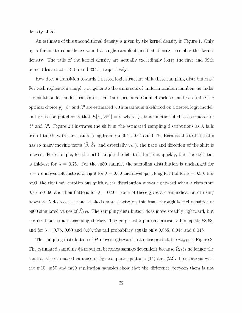
How does a transition towards a nested logit structure shift these sampling distributions?

For each replication sample, we generate the same sets of uniform random numbers as under

the multinomial model, transform them into correlated Gumbel variates, and determine the

optimal choice yj. β0 and λ0 are estimated with maximum likelihood on a nested logit model,

and βa is computed such that E[gC(βa)] = 0 where gC is a function of these estimates of

β0 and λ0. Figure 2 illustrates the shift in the estimated sampling distributions as λ falls

from 1 to 0.5, with correlation rising from 0 to 0.44, 0.64 and 0.75. Because the test statistic

has so many moving parts (β, βD and especially yDr), the pace and direction of the shift is

uneven. For example, for the m10 sample the left tail thins out quickly, but the right tail

is thickest for λ = 0.75. For the m50 sample, the sampling distribution is unchanged for

λ = 75, moves left instead of right for λ = 0.60 and develops a long left tail for λ = 0.50. For

m90, the right tail empties out quickly, the distribution moves rightward when λ rises from

0.75 to 0.60 and then flattens for λ = 0.50. None of these gives a clear indication of rising

power as λ decreases. Panel d sheds more clarity on this issue through kernel densities of

5000 simulated values of H123. The sampling distribution does move steadily rightward, but

the right tail is not becoming thicker. The empirical 5-percent critical value equals 58.63,

and for λ = 0.75, 0.60 and 0.50, the tail probability equals only 0.055, 0.045 and 0.046.

The sampling distribution of H moves rightward in a more predictable way; see Figure 3.

The estimated sampling distribution becomes sample-dependent because ΩD is no longer the

same as the estimated variance of δD; compare equations (14) and (22). Illustrations with

the m10, m50 and m90 replication samples show that the difference between them is not

22

0

0.01

0.02

0.03

0.04

-60 -40 -20 0 20 40 60

f(H)

H

Null

NL: λ=0.75

NL: λ=0.60

NL: λ=0.50

a: Replication sample m10

0

0.01

0.02

0.03

0.04

-60 -40 -20 0 20 40 60

f(H)

H

Null

NL: λ=0.75

NL: λ=0.60

NL: λ=0.50

b: Replication sample m50

0

0.01

0.02

0.03

0.04

-60 -40 -20 0 20 40 60

f(H)

H

Null

NL: λ=0.75

NL: λ=0.60

NL: λ=0.50

c: Replication sample m90

0

0.01

0.02

0.03

0.04

-60 -40 -20 0 20 40 60

f(H)

H

Null

NL: λ=0.75

NL: λ=0.60

NL: λ=0.50

d: Kernel density

Figure 2: Density functions of H under the null and alternative hypotheses

trivial, but in view of the critical value of 30.39, power clearly rises with falling λ for every

replication sample. The kernel density illustrates the steady shift rightward as λ decreases.

Note also that the density under the null hypothesis is not much different from the χ2 density

(dotted gray curve), even though the goodness of fit test (Table 5) pointed out a significant

difference.

23

0.00

0.01

0.02

0.03

0.04

0.05

0.06

0.07

0 20 40 60 80

f(H)

H

Null

NL: λ=0.75

NL: λ=0.60

NL: λ=0.50

a: Replication sample m10

0.00

0.01

0.02

0.03

0.04

0.05

0.06

0.07

0 20 40 60 80

f(H)

H

Null

NL: λ=0.75

NL: λ=0.60

NL: λ=0.50

b: Replication sample m50

λ=0.75

λ=0.60

λ=0.50

0.00

0.01

0.02

0.03

0.04

0.05

0.06

0.07

0 20 40 60 80

f(H)

H

Null

NL: λ=0.75

NL: λ=0.60

NL: λ=0.50

c: Replication sample m90

0

0.01

0.02

0.03

0.04

0.05

0.06

0.07

0 20 40 60 80

f(H)

H

Null

NL: λ=0.75

NL: λ=0.60

NL: λ=0.50

χ2

d: Kernel density

Figure 3: Density functions of H under the null and alternative hypotheses

5 A sandwich version of the HM test

The Hs test of Weesie (1999) replaces VD in equation (14) with a sandwich estimator, as an

application of a technique that applies more generally to tests on different sets of parameters

that are drawn from the same sample. Thus, use Taylor expansions as in equations (17) and

(18), and write the parameter vectors as

β − β0

βD − β0D

= −

hC(β0)−1 0

0 hD(β0D)−1

gC(β0)

gC(β0D)

(23)

24

Let gCi and gDi be the gradients of the respective log-likelihood functions for observation i.

Then, the sandwich estimator of VD is given by

V sD =

hC(β)−1 0

0 hD(βD)−1

n∑i=1

gCi(β)

gDi(βD)

gCi(β)

gDi(βD)

′ hC(β)−1 0

0 hD(βD)−1

(24)

Asymptotically, the middle term simplifies to an expression similar to that in equation (22)

evaluated at β0 and β0D, which underlies VD in equation (14). In small samples, the sandwich

estimator V sD may deviate from VD, which will cause the distribution of Hs to deviate from

that of H. Monte Carlo analysis must give insight into how large this deviation may be.

Table 8 shows size of Hs and must be compared with Table 5 for H. In small samples,

Hs suffers from serious size distortions: for example, the actual size at a nominal size of 5

percent is frequently below 1 percent. Even for large samples, the actual size is no larger

than 3.8 percent. Thus, the critical value given by the χ2 distribution is too high. The large

goodness of fit statistics highlight the gap between the distribution of Hs and the asymptotic

χ2 distribution.

This size distortion leads to substantial underrejection of the Null hypothesis. For J = 4

with a small-sample Set 3, in the cases with D = 12, D = 123 and D = 234 when

the nesting structure with λ = 0.50 is correctly specified, we find nominal power equal to

0.063, 0.065 and 0.043, respectively, whereas actual power is 0.176, 0.247 and 0.240 (Table

9, lower left block). However, these are substantially below the power of H in same three

cells of Table 7, equal to 0.595, 0.816, and 0.763, respectively. With a few exceptions, the

power of Hs is lower than that of H when the Null hypothesis represents the correlation

structure correctly. And in 17 out of 36 instances in Table 9, Hs has more power when the

correlation structure is misspecified than when it is correctly specified, which will likely lead

the researcher to select the wrong nesting structure.

25

0

0.01

0.02

0.03

0.04

0.05

0.06

0.07

0.08

0 20 40 60 80

H-hat (Null)

H-s (Null)

χ2

H-hat (λ=0.5)

H-s (λ=0.5)

f(H)

H

Figure 4: Comparing kernel density functions of H and Hs under Null and Alternativehypotheses (Set 3, small sample, J = 4, D = 123)

The divergence between H and Hs is well demonstrated in Figure 4. Solid density curves

refer to H, dashed curves to Hs, and the dotted curve to the χ2 distribution. Under the

Null, the gap between the density of Hs and the χ2 curve is pronounced. When λ decreases

from 1 (IIA) to 0.50, the pdf of Hs moves only gingerly to the right, whereas the pdf of H

slides a large distance rightward.

Overall, therefore, the Hs test addresses the main shortcoming of the traditionally applied

HM test for IIA by preventing indefinite estimated covariance matrices and negative H

outcomes, but the size distortion of Hs leads to many type-II errors in inference, unless the

proper critical value is computed by simulation. Moreover, Hs is dominated by H.

26

6 An application

The Ivorian data that are the basis for Set 3 of the simulation study offers a good contrast

between the three versions of the HM test. The employment choices are: 1=farming, 2=non-

farm self-employment, 3=wage employment, and 4=non-employment. Is MNL a good model

to understand employment outcomes, or is the IIA assumption too restrictive?

Table 10 shows tests for IIA for every possible specification of D on the basis of H, H

and Hs. Five of the H outcomes are large in the light of their χ2 distribution; four H’s are

negative; and none of the ˘ΩD matrices is positive definite. Size correction of the p-values of

H narrows the options: D = 234 or perhaps D = 34 looks to be a good selection, but

one might wonder what the H124 outcome in the far left tail signifies.

The H tests come to a different conclusion: D = 12 draws the largest H value and the

smallest p-value, rejecting IIA in favor of a nesting of outcomes 1 and 2 if the nested logit is

to be adopted. A nesting of D = 124 might also be considered.

Interestingly, the Hs tests feature two examples (Hs13 and Hs

234) where the asymptotic p-

value leads to non-rejection at a 5-percent significance level but the simulated p-value dictates

rejection. Based on p-values, the Hs tests suggest nesting either D = 12 or D = 123;

Hs124 is also statistically significant but not as large as Hs

123.

The last column of Table 10 reports the estimates of the nesting parameter λ for each

nesting structure. The nested logit model that nests outcomes 1 and 2 yields λ = 2.97,

outside the range (0, 1). In fact, for nine selections of D, λ exceeds 1, and for the tenth

(D = 134) it equals only 0.93, too close to 1 for a meaningful nesting structure. Thus,

despite the rejection of IIA by the H and Hs tests, the nested logit model may not be the

right econometric model for activity choice in Cote d’Ivoire. Indeed, that the alternative

hypothesis of the HM test is quite general (Train, 2009): the correct alternative model need

not be a nested logit model.

27

0

0.01

0.02

0.03

0.04

0.05

0.06

0.07

-60 -40 -20 0 20 40 60

n=1480

n=7400

n=25000

n=100000

χ2

H

f(H)

Figure 5: Kernel density functions of H under IIA for increasing sample sizes (Set 3, J = 4,D = 123)

7 Concluding remarks

The simulation and analytical results presented in this paper provide convincing evidence

that the distribution of the traditional implementation of the HM test through H deviates

greatly from the asymptotic χ2 distribution.

One might contend that the sample sizes in the Monte Carlo simulations were too small

to permit substitution of asymptotic distributions. Figure 5 extends the sample size for Set

3 with D = 123. The sampling distribution is moving towards χ2, but for n = 25180

observations the goodness of fit test equals 1345 (exceeding χ20.99 = 36.19), the chance of

a negative H equals 11.4 percent, and 91.3 percent of the ˘ΩDr are indefinite. Even for

n = 100640 observations, discrepancies remain large: the goodness of fit test equals 523,

28

the chance of a negative H equals 5.2 percent, and 59.7 percent of the ˘ΩDr are indefinite.

Meanwhile, the sampling distribution of H is indistinguishable from χ2 for n = 7400 and

deviates only little for n = 1480 (goodness of fit test equals 51).

The conclusions are clear. In its commonly applied form (H), the HM test for IIA that

has been the favorite among applied researchers over the past 26 years sometimes generates

negative values—or a kind warning by the software package that the covariance matrix is not

positive definite. It is time to take these signals seriously. These problems arise because of

an improper conceptualization of the covariance matrix and imply that, as a rule, the small-

sample distribution of H deviates dramatically from the χ2 distribution: negative test values

are common, and violations of IIA may in fact yield large negative test values.20 In other

words, judging the outcome of the standard HM test by the upper tail of a χ2 distribution is

likely to lead to an incorrect statistical inference. Given that there are at least 276 studies in

the literature with 433 applications of the standard HM test, these findings put a significant

body of empirical research at risk.

The conceptually correct implementation of the test, H, is distributed approximately

as χ2 in small samples, in principle without the occurrence of negative outcomes although

singularity of the covariance matrix may occasionally be an issue. H and H are nearly

uncorrelated, but other statistics that are available in a simulation study such as this strongly

suggest that H is a more reliable test instrument than H. Weesie’s (1999) sandwich version

of the HM test, Hs, offers an alternative approach to address the same shortcomings of H

but is dominated in our simulations by H. Thus, if researchers want to test for IIA with the

Hausman-McFadden test, they should abandon H and use H.

20For any given sample where it is unknown whether IIA is violated, the fact that the sampling distributionis sample-dependent implies that the density function under the null hypothesis is in fact unknown becausebehavior of sample members under certifiable IIA is not observed.

29

Appendices

A Comparing Σ0Dr with Σ0

D in large samples

Denote individuals by the double subscript it with i = 1, . . . , n and t = 1, . . . , T . Instead of

letting n go to ∞, consider gathering T samples of n individuals each, one of each type i,

such that Xit = Xi for all t, with T going to ∞. This simplifying assumption is adequate

for the purpose at hand. Then TΣ0D equals the inverse of − 1

TE[h0D(β0

D)]. Block j, k of this

expression equals

1

TE0

[∂2 lnLD(β0

D)

∂βj∂β′k

]= − 1

T

T∑t=1

n∑i=1

p0jit(I(j = k)− q0kit

)XitX

′it (A.1)

which, since by assumption Xit = Xi and thus also pjit = pji and qkit = qki for all t, is the

same as equation (10).

As for T Σ0Dr, rewriting equation (11) in a similar way yields

1

T

∂2 ln LD(β0D)

∂βj∂β′k= − 1

T

T∑t=1

n∑i=1

yDitq0jit

(I(j = k)− q0kit

)XitX

′it (A.2)

= −n∑i=1

(1

T

T∑t=1

yDit

)q0ji(I(j = k)− q0ki

)XiX

′i. (A.3)

Because 1T

∑Tt=1 yDit converges to p0Di as T → ∞, and since p0Diq

0ji = p0ji, the expression in

equation (A.3) converges to that in equation (10). Thus, T Σ0Dr converges to TΣ0

D. As β

converges to β0 and βD converges to β0D, T ˘ΣDr also converges to TΣ0

D.

B ΩD is positive definite for any β

Without loss of generality, assume that the restricted choice set D contains the base category,

and define D† as the complement of D. Reorder β such that β =(β′D† , β

′D

)′, such that

30

the parameters associated with D appear at the bottom; note that βJ = 0 because of

standardization. Thus, let D† = 1, . . . , j1 and D = j2, . . . , J with j2 = j1 + 1. Restate

the variance of β as

ΣC =

(−E

[∂2 lnLC∂β∂β′

])−1=

−A11 −A12

−A21 −A22

−1

(B.1)

which means that ΣC,DD =(−A22 + A21A

−111 A12

)−1. Define Πj = diag(p0.5ji ), Θ1 = (Π1 . . . Πj1)

′,

Θ2 = (Πj2 . . . ΠJ−1)′, ΠD = diag(p0.5Di) and Π∗j = ΠjΠ

−1D . Then, let Z1 = diag(Θ1) (Ij1 ⊗X)

and Z2 = diag(Θ2) (IJ−j2 ⊗X). Given equation (4) of Section 4.1, this allows us to write

A11 = Z1 (Θ1Θ′1 − Inj1)Z1, A12 = A′21 = Z1Θ1Θ

′2Z2, and A22 = Z2

(Θ2Θ

′2 − In(J−j2)

)Z2.

Furthermore, restate the variance of βD as

ΣD =

(−E

[∂2 lnLD∂βD∂β′D

])−1= −A−122 (B.2)

with block j, k of A22 equal to:

A22,jk = E

[∂2 lnLD∂βj∂β′k

]=

n∑i=1

(pjipkipDi

− pjiI(j = k)

)XiX

′i (B.3)

which implies that A22 = Z ′2(Θ2Π

−2D Θ′2 − In(J−j2)

)Z2.

Next, consider that ΩD > 0 if ΣD > ΣC,DD, i.e., if A−122 <(A22 − A21A

−111 A12

)−1, and

thus if A22 − A22 + A21A−111 A12 > 0. From the definitions above, we have A22 − A22 =

Z ′2Θ2

(Π−2D − In

)Θ′2Z2. As for the other term, write Inj1 −Θ1Θ

′1 = V , such that

A21A−111 A12 = −Z ′2Θ2Θ

′1Z1 (Z ′1V Z1)

−1Z ′1Θ1Θ

′2Z2

= −Z ′2Θ2Θ′1V−0.5

(V 0.5Z1 (Z ′1V Z1)

−1Z ′1V

0.5)V −0.5Θ1Θ

′2Z2 (B.4)

31

As it happens, V is a symmetric nj1×nj1 matrix that counts Θ1 (Θ′1Θ1)−1 among its eigen-

vectors, with eigenvalues Λ1 = (Θ′1Θ1)−1 − In. From the definition of Θ1, it follows that

Θ′1Θ1 = diag(∑j1

j=1 pji

)= diag(1 − pDi) = In − Π2

D and therefore Λ1 = Π2D (In − Π2

D)−1

.

Moreover, V −0.5Θ1 = Θ1 (In − Π2D)

0.5Π−1D ≡ Θ1Λ

∗1. Substitution of these results into equa-

tion (B.4) yields

A22 − A22 + A21A−111 A12 = Z ′2Θ2

(Π−2D − In

)Θ′2Z2 − Z ′2Θ2Λ

∗1Θ′1Θ1Λ

∗1Θ′2Z2

+ Z ′2Θ2Λ∗1Θ′1

(Inj1 − V 0.5Z1 (Z ′1V Z1)

−1Z ′1V

0.5)

Θ1Λ∗1Θ′2Z2 (B.5)

The second line of equation (B.5) is a quadratic form around a idempotent matrix and is

therefore positive semidefinite. With the insertion of Θ′1Θ1 = In−Π2D, the first line simplifies

to Z ′2Θ2 (In − Π2D) Θ′2Z2, which is positive definite. Thus, ΩD is positive definite, and this is

true for any β.

C β under conditional sampling

With conditional sampling, the properties of β are assessed under the assumption that the

randomness of β arises from assigning draws of εji to all members of sample Sr such that

members of subsample Sr(D) will always again choose an outcome from D and members of

subsample Sr(D†) will always again choose an outcome from D†. We refer to this as sampling

strategy r. In other words, this strategy is dictated by the outcome of the once-drawn random

sample of a given research project.

Maximizing lnLC in equation (2) yields the first order condition

gC(β) =n∑i=1

∑j∈C

(yji − pji)Xi (C.1)

32

where probability pji is evaluated at β. Take a Taylor expansion around β0:

(β − β0

)= −hC(β0)−1gC(β0) (C.2)

where hC(β0) is given in equation (4). Under conditional sampling with sampling strategy

r, we have:

E [yji|r] =

pji

1−pDifor j ∈ D† and i ∈ Sr(D†)

pjipDi

for j ∈ D and i ∈ Sr(D)

0 otherwise

With this, the conditional mean of gC(β0) under sampling strategy r equals

E [gC(β)|r] =n∑i=1

∑j∈C

ajipjiXi (C.3)

where

ayji =

pji

1−pDifor j ∈ D† and i ∈ Sr(D†)

pjipDi

for j ∈ D and i ∈ Sr(D)

−1 otherwise

Unconditionally, E [gC(β)] equals 0, but conditional on sampling strategy r, E [gC(β)|r] does

not equal 0 unless by coincidence. Thus, E[β − β0|r)

]6= 0.

Next, consider the question of whether β is consistent. As in Appendix A, let there be

n types of individuals; draw T individuals of each type to constitute a enlarged sample;

and denote individuals by the double subscript it with i = 1, . . . , n and t = 1, . . . , T . To

examine consistency, gather T samples of n individuals each, one of each type i, such that

Xit = Xi for all t, with T going to ∞, with the condition that the proportion of the sample

that chooses an outcome from set D remains the same as in the original sample Sr. In this

original sample, let n1r be the number of members of subsample Sr(D). Let N = nT be the

size of the enlarged sample, and let N1 be the number of members of the enlarged sample

33

that chooses j ∈ D. Then N1/N must remain equal to n1r as T →∞. Since the probability

of a person of type i choosing j ∈ D equals p0Di, the expected proportion of sample members

choosing j ∈ D equals p0 = 1n

∑ni=1 p

0Di where p0Di is evaluated at β0. This is true also in the

enlarged sample as T →∞. Unconditionally, N1/N converges to p0, but with the condition

of sampling strategy r, N1/N must equal n1r. Thus, with pDi evaluated at β as T → ∞,

p = 1n

∑ni=1 pDi must equals n1r. Unless by chance we have n1r = p0 in the original sample,

β has no chance to converge to β0 as T → ∞. Thus, generally, β is inconsistent under

sampling strategy r.

D Tests for normality

In a test of joint normality, three features of the simulated parameter estimates matter: is

their mean close to the theoretical mean; is their covariance matrix close to the theoretical

variance, and is the shape of the distribution close to normality? Table D1 examines the

simulated parameter values for each set for J = 3 and J = 4, for the estimator of the MNL

model with the overall choice set C (β) and with one or two versions of a restricted choice

set D (βD) and for the difference δD that is the immediate focus of the Hausman-McFadden

test.

Bias in the mean and variance is tested by means of a likelihood ratio test. For example,

if the draws βr are distributed N(β0,Σ0C), one may “estimate” β0 and Σ0

C by maximum

likelihood from the simulated sample β1, . . . , βR and then observe by a likelihood ratio

test whether the true β0 and Σ0C fairly represent the mean and variance of β. In Table

D1, LR(mean) inserts the covariance among the simulated sample for Σ0C and tests whether

E[βr] = β0. LR(var) inserts the mean of the simulated sample for β0 and tests whether

the simulated covariance equals Σ0C . The bias in the mean is usually more pronounced than

the bias in the variance, but especially for δD the variance of the simulated draws deviates

greatly from ΩD.

34

The shape of the distribution is examined with the test designed by Doornik and Hansen

(2008), which considers skewness and kurtosis of each element of the parameter vector

through a joint test statistic. Virtually without fail, joint normality is rejected. For ele-

ments of δD, while skewness is sometimes to the left and other times to the right, every

element is more peaked than normality, which also means that tails are more extended.

E Singularity of ΩD

As shown in Appendix B, ΩD is a positive definite matrix, regardless of the value of β for

which ΩD is evaluated. Nevertheless, during the simulations, a few negative values showed

up for H. Mathematically, this is impossible, but one would have to suspect that numerical

errors are to blame for this.

Let us consider this idea. First of all, one would think that H is more or less quadratic

in δD = βD − βD, but ΩD is of course a complicated function of β. Let us therefore examine

the values of H along a ray from β0 through β and βD: see Figure E.1. Thus, we evaluate H

at β = (1− θ)β0 + θβ, where θ varies from 0 to 2: for θ = 1, the Monte Carlo value obtains,

and for θ = 0, we have H = 0. For this we select two of the 5000 random samples of the

Monte Carlo analysis for Set 1, small sample, with J = 4. Sample r1 yields H34 = 3.57 and

H134 = 4.81, both of which are less than the 5-percent asymptotic critical value (χ20.95(3) =

7.81 and χ20.95(6) = 12.59. Figure E.1 shows a quadratic reference line through the Monte

Carlo value at θ = 1, which holds ΩD fixed. But clearly, H does not behave quadratically. In

fact, if β were estimated closer to β0, at around θ = 0.45, H34 would be judged statistically

significant. Moreover, the small value of H134 at θ = 1 seems fortuitous: the behavior of

H134 is highly erratic, to say the least.

For sample r2, the Monte Carlo values equal H34 = −13.09 and H134 = 1.31: along the

ray, both statistics behave erratically. For H34, |ΩD| drops below 10−18 at θ = 1, and for

35

0

2

4

6

8

10

12

14

16

0 0.5 1 1.5 2

H_h

at f

or

D=3

4

(a) Estimate r1: D = 34

-60

-40

-20

0

20

40

60

0 0.5 1 1.5 2

H_h

at f

or

D=1

34

(b) Estimate r1: D = 134

-60

-40

-20

0

20

40

60

0 0.5 1 1.5 2

H_h

at f

or

D=3

4

(c) Estimate r2: D = 34

-60

-40

-20

0

20

40

60

0 0.5 1 1.5 2

H_h

at f

or

D=1

34

(d) Estimate r2: D = 134

Figure E.1: H along a ray from β0 to 2β for two sets of estimates of β.

Note: The position on the ray is indicated by θ on the horizontal axis. Along the ray, β = (1 − θ)β0 + θβ.

The gray curve uses Ω(β), whereas the black line uses Ω(β). Values of H are truncated at 50 and −50 to

preserve the scale of the graphs.

36

H134, |ΩD| is always smaller than 10−35.21 Clearly, singularity of ΩD is playing a role.

References

Cheng, S., and J. S. Long (2007): “Testing for IIA in the Multinomial Logit Model,”Sociological Methods and Research, 35(4), 583–600.

Doornik, J. A., and H. Hansen (2008): “An omnibus test for univariate and multivariatenormality,” Oxford Bulletin of Economics and Statistics, 70(Supp.1), 927–939.

Fry, T. R. L., and M. N. Harris (1996): “A Monte Carlo study of tests for the Inde-pendence of Irrelevant Alternatives property,” Transportation Research Part B: Method-ological, 30(1), 19–30.

(1998): “Testing for Independence of Irrelevant Alternatives: some empirical re-sults,” Sociological Methods and Research, 26(3), 401–423.

Hausman, J. (1978): “Specification Tests in econometrics,” Econometrica, 46(6), 1251–1271.

Hausman, J., and D. McFadden (1984): “Specification Tests for the Multinomial LogitModel,” Econometrica, 52(5), 1219–1240.

Imhof, J. P. (1961): “Computing the distribution of quadratic forms in normal variables,”Biometrika, 48(3/4), 419–426.

McFadden, D. (1987): “Regression-based specification tests for the Multinomial Logitmodel,” Journal of Econometrics, 34(1-2), 63–82.

McFadden, D., K. Train, and W. Tye (1977): “An application of diagnostic tests forthe Independence of Irrelevant Alternatives property of the Multinomial Logit model,”Transportation Research Record, 637, 39–46.

Small, K. A. (1994): “Approximate generalized extreme value models of discrete choice,”Journal of Econometrics, 62(2), 351–382.

Small, K. A., and C. Hsiao (1985): “Multinomial Logit specification tests,” InternationalEconomic Review, 26(3), 619–627.

Train, K. E. (2009): Discrete Choice Methods with Simulation. New York: CambridgeUniversity Press, 2 edn.

21The careful observer may note that H34 along the curve does not pass through the Monte Carlo value of−13.09 but rather equals 4.47. The curve is generated with a grid search of width 0.01: the mere recalculationof ΩD at a value of β that might differ in the sixth or seventh decimal already generates a different outcome.

37

Vijverberg, W. P. M. (1993): “Educational investments and returns for women and menin Cote d’Ivoire,” Journal of Human Resources, 28(4), 933–974.

Weesie, J. (1999): “Seemingly unrelated estimation and the cluster-adjusted sandwichestimator,” Stata Technical Bulletin, 52, 34–47.

Zhang, J., and S. D. Hoffman (1993): “Discrete-Choice Logit Models: Testing the IIAproperty,” Sociological Methods & Research, 22(2), 193–213.

Zheng, X. (2008): “Testing for discrete choice models,” Economics Letters, 98(2), 176–184.

38

Table 1. Use of the Hausman-McFadden test in the literature, 1984-2010

1985-2004 2005-2010 TotalNumber Percent Number Percent Number Percent

A: Number of tested models

Reports all positive test valuesFails to reject IIA 79 35.4 69 32.9 148 34.2Rejects IIA 34 15.2 42 20.0 76 17.6Total 113 50.7 111 52.9 224 51.7

Reports at least one negative test valueFails to reject IIA 23 10.3 19 9.0 42 9.7Rejects IIA 5 2.2 2 1.0 7 1.6Draws no conclusion 7 3.1 0 0.0 7 1.6Use modified HM test statistic 9 4.0 5 2.4 14 3.2Total 44 19.7 26 12.4 70 16.2

Describes test outcome verballyFails to reject IIA 48 21.5 55 26.2 103 23.8Rejects IIA 18 8.1 18 8.6 36 8.3Total 66 29.6 73 34.8 139 32.1

Total 223 100.0 210 100.0 433 100.0

B: Number of studies that cite Hausman and McFadden (1984)

Implementing the HM test 136 140 276Citing for its theoretical/

conceptual contribution 34 13 47Citing without apparent

theoretical/conceptual contribution 45 16 61Incorrectly included in Web of Science: 3 1 4Total number of studies 218 170 388

Source: Web of Science, accessed in March-June 2005 and February 2010, in a search for studies that citeHausman and McFadden (1984). One study in 1992 is added that cited an earlier working paper.

39

Table 2. Characteristics of Monte Carlo Data Sets

J = 3 J = 4Min Mean Max St.Dev. Min Mean Max St.Dev.

Set 1 (N = 1000)p1 0.234 0.614 0.886 0.118 0.211 0.565 0.853 0.120p2 0.039 0.246 0.643 0.106 0.037 0.225 0.593 0.097p3 0.051 0.140 0.322 0.041 0.015 0.084 0.304 0.042p4 ... ... ... ... 0.050 0.127 0.225 0.030

Set 2 (N = 1000)p1 0.397 0.519 0.961 0.090 0.112 0.328 0.958 0.130p2 0.001 0.117 0.284 0.048 0.001 0.071 0.229 0.035p3 0.038 0.364 0.529 0.069 0.003 0.387 0.719 0.129p4 ... ... ... ... 0.038 0.215 0.236 0.020

Set 3 (N = 1118 for J = 3, N = 1480 for J = 4)p1 0.004 0.233 0.872 0.202 0.004 0.176 0.722 0.162p2 0.008 0.275 0.947 0.219 0.008 0.208 0.927 0.193p3 0.020 0.491 0.983 0.291 0.015 0.371 0.971 0.286p4 ... ... ... ... 0.004 0.245 0.831 0.265

40

Table 3: Behavior of H under the Null hypothesis

Small samplea Large sampleb

Empirical size at Goodness Empirical size at Goodnessa nominal size of of fit a nominal size of of fit

D 0.10 0.05 0.01 χ2(19)c 0.10 0.05 0.01 χ2(19)c

A: J = 3

Set 1 12 0.153 0.103 0.049 343 0.106 0.053 0.010 1813 0.368 0.309 0.221 7168 0.180 0.118 0.051 53623 0.323 0.268 0.178 5130 0.154 0.100 0.037 301

Set 2 12 0.263 0.202 0.126 2495 0.136 0.083 0.028 12913 0.277 0.221 0.147 3241 0.137 0.087 0.035 18423 0.406 0.346 0.250 9395 0.179 0.123 0.054 607

Set 3 12 0.224 0.152 0.068 1216 0.113 0.063 0.015 3513 0.203 0.138 0.062 902 0.118 0.060 0.015 3623 0.193 0.129 0.051 746 0.113 0.062 0.012 31

B: J = 4

Set 1 12 0.166 0.112 0.053 432 0.105 0.056 0.014 25123 0.366 0.298 0.200 6672 0.149 0.091 0.031 230234 0.872 0.852 0.814 67808 0.586 0.533 0.432 24659

Set 2 12 0.326 0.269 0.188 5164 0.151 0.094 0.037 231123 0.391 0.325 0.232 8143 0.165 0.099 0.036 329234 0.596 0.539 0.426 25373 0.241 0.172 0.089 1677

Set 3 12 0.232 0.162 0.080 1474 0.126 0.066 0.017 68123 0.264 0.190 0.089 2271 0.136 0.077 0.024 143234 0.267 0.186 0.090 2236 0.138 0.082 0.023 145

a N = 1000 for Sets 1 and 2; for Set 3, N = 1118 for J = 3 and N = 1480 for J = 4,b N = 7500 for Sets 1 and 2; for Set 3, N = 7826 for J = 3 and N = 7400 for J = 4.c Critical values are 27.20 (10 percent), 30.14 (5 percent) and 36.19 (1 percent).

41

Table 4: Behavior of H under the Null hypothesis

Empirical size at Goodness

a nominal size of Indefinite ˘ΩDr of fit

D 0.10 0.05 0.01 H ≤ 0 H > 0 Total χ2(19)a

A1: J = 3, Small sampleb

Set 1 12 0.045 0.039 0.027 0.408 0.352 0.760 391813 0.023 0.020 0.012 0.407 0.400 0.807 835723 0.044 0.035 0.024 0.380 0.323 0.703 4082

Set 2 12 0.041 0.034 0.027 0.344 0.572 0.916 976613 0.001 0.001 0.001 0.589 0.382 0.971 1633323 0.033 0.026 0.020 0.395 0.513 0.908 10661

Set 3 12 0.108 0.097 0.077 0.502 0.485 0.987 465513 0.168 0.147 0.114 0.401 0.530 0.930 404523 0.116 0.101 0.080 0.478 0.504 0.982 4341

A2: J = 3, Large samplec

Set 1 12 0.105 0.083 0.056 0.155 0.406 0.561 130413 0.083 0.068 0.048 0.249 0.459 0.708 324623 0.112 0.090 0.059 0.149 0.409 0.558 1375

Set 2 12 0.089 0.073 0.051 0.281 0.502 0.782 310113 0.012 0.011 0.008 0.561 0.381 0.942 1020823 0.105 0.087 0.064 0.288 0.505 0.793 3204

Set 3 12 0.292 0.240 0.171 0.091 0.414 0.504 422713 0.213 0.166 0.099 0.076 0.328 0.405 175323 0.277 0.231 0.162 0.082 0.381 0.464 3863

B1: J = 4, Small sampled

Set 1 12 0.066 0.054 0.038 0.384 0.362 0.746 3019123 0.045 0.038 0.027 0.422 0.507 0.930 11966234 0.037 0.029 0.022 0.284 0.593 0.877 18242

Set 2 12 0.056 0.048 0.034 0.337 0.574 0.911 7945123 0.059 0.051 0.040 0.473 0.506 0.979 9743234 0.026 0.022 0.018 0.426 0.550 0.976 18053

Set 3 12 0.153 0.135 0.109 0.428 0.533 0.961 4199123 0.106 0.097 0.084 0.471 0.529 1.000 9185234 0.085 0.077 0.062 0.563 0.437 1.000 7325

B2: J = 4, Large samplee

Set 1 12 0.111 0.084 0.051 0.138 0.403 0.541 1086123 0.099 0.085 0.061 0.127 0.756 0.883 8995234 0.044 0.034 0.025 0.173 0.696 0.869 15706

Set 2 12 0.101 0.081 0.056 0.256 0.519 0.775 2652123 0.122 0.098 0.072 0.145 0.806 0.950 6532234 0.102 0.087 0.066 0.247 0.710 0.957 9372

Set 3 12 0.279 0.231 0.162 0.090 0.380 0.470 3876123 0.222 0.199 0.156 0.239 0.758 0.997 6635234 0.238 0.214 0.175 0.272 0.726 0.998 6824

a Critical values are 27.20 (10 percent), 30.14 (5 percent) and 36.19 (1 percent).b N = 1000 for Sets 1 and 2; N = 1118 for Set 3.c N = 7500 for Sets 1 and 2; N = 7826 for Set 3.d N = 1000 for Sets 1 and 2; N = 1480 for Set 3.e N = 7500 for Sets 1 and 2; N = 7400 for Set 3.

42

Table 5: Behavior of H under the Null hypothesis

Small samplea Large sampleb

Empirical size at Goodness Empirical size at Goodnessa nominal size of of fit a nominal size of of fit

D 0.10 0.05 0.01 χ2(19)c 0.10 0.05 0.01 χ2(19)c

A: J = 3

Set 1 12 0.094 0.049 0.015 22 0.096 0.045 0.007 2313 0.105 0.053 0.015 15 0.101 0.053 0.011 2523 0.107 0.060 0.017 25 0.100 0.049 0.014 12

Set 2 12 0.099 0.053 0.016 22 0.104 0.050 0.012 1913 0.083 0.043 0.016 139 0.097 0.050 0.017 4323 0.107 0.057 0.015 28 0.102 0.049 0.011 31

Set 3 12 0.115 0.066 0.017 50 0.100 0.051 0.010 1513 0.122 0.066 0.017 49 0.112 0.054 0.008 2523 0.114 0.062 0.016 21 0.100 0.050 0.010 10

B: J = 4

Set 1 12 0.099 0.053 0.013 20 0.093 0.046 0.010 18123 0.104 0.061 0.019 56 0.097 0.049 0.011 15234 0.134 0.081 0.031 128 0.098 0.054 0.011 35

Set 2 12 0.116 0.070 0.024 64 0.101 0.052 0.010 21123 0.115 0.067 0.020 59 0.100 0.048 0.009 14234 0.107 0.058 0.013 33 0.105 0.053 0.012 18

Set 3 12 0.138 0.077 0.023 104 0.106 0.052 0.012 26123 0.122 0.068 0.014 51 0.106 0.052 0.014 26234 0.115 0.062 0.016 36 0.109 0.055 0.012 17

a N = 1000 for Sets 1 and 2; for Set 3, N = 1118 for J = 3 and N = 1480 for J = 4,b N = 7500 for Sets 1 and 2; for Set 3, N = 7826 for J = 3 and N = 7400 for J = 4.c Critical values are 27.20 (10 percent), 30.14 (5 percent) and 36.19 (1 percent).

43

Table 6: Size-adjusted power of H for three nesting structures

D Power H ≤ 0 ˘ΩDr is indefinite(12)3 2(13) 1(23) (12)3 2(13) 1(23) (12)3 2(13) 1(23)

A1: J = 3, Small sample

Set 1 12 0.074 0.023 0.021 0.195 0.527 0.500 0.369 0.866 0.84813 0.074 0.170 0.190 0.441 0.210 0.198 0.867 0.764 0.76423 0.177 0.072 0.083 0.292 0.276 0.279 0.723 0.764 0.764

Set 2 12 0.051 0.043 0.095 0.197 0.407 0.238 0.905 0.932 0.93413 0.006 0.284 0.011 0.632 0.482 0.621 0.990 0.914 0.98123 0.096 0.043 0.070 0.238 0.468 0.283 0.912 0.910 0.861

Set 3 12 0.026 0.085 0.065 0.050 0.668 0.621 0.113 0.995 0.98913 0.091 0.007 0.050 0.525 0.012 0.566 0.983 0.018 0.99523 0.026 0.048 0.036 0.617 0.644 0.017 0.999 1.000 0.026

A2: J = 3, Large sample

Set 1 12 0.053 0.072 0.057 0.008 0.273 0.291 0.010 0.718 0.70313 0.099 0.025 0.027 0.276 0.224 0.222 0.894 0.507 0.50923 0.140 0.039 0.045 0.116 0.223 0.216 0.828 0.713 0.704

Set 2 12 0.022 0.055 0.063 0.261 0.294 0.214 0.746 0.836 0.90813 0.001 0.397 0.012 0.578 0.300 0.610 0.973 0.646 0.97323 0.029 0.056 0.028 0.209 0.325 0.250 0.862 0.792 0.500

Set 3 12 0.000 0.456 0.353 0.000 0.428 0.355 0.000 0.999 0.96613 0.737 0.875 0.478 0.068 0.000 0.068 0.975 0.000 1.00023 0.093 0.276 0.038 0.602 0.420 0.000 0.897 1.000 0.000

(12)34 (123)4 1(234) (12)34 (123)4 1(234) (12)34 (123)4 1(234)

B1: J = 4, Small sample

Set 1 12 0.048 0.047 0.053 0.164 0.193 0.547 0.324 0.396 0.887123 0.065 0.070 0.098 0.226 0.155 0.396 0.840 0.845 0.990234 0.104 0.135 0.070 0.277 0.310 0.102 0.940 0.942 0.686

Set 2 12 0.027 0.037 0.066 0.220 0.219 0.213 0.892 0.855 0.957123 0.058 0.053 0.089 0.397 0.093 0.430 0.980 0.912 0.996234 0.067 0.176 0.120 0.353 0.428 0.206 0.990 0.996 0.943

Set 3 12 0.012 0.046 0.078 0.030 0.113 0.450 0.058 0.236 0.932123 0.073 0.045 0.060 0.402 0.127 0.574 1.000 0.770 1.000234 0.048 0.049 0.101 0.530 0.687 0.129 1.000 1.000 0.582

B2: J = 4, Large sample

Set 1 12 0.124 0.045 0.256 0.002 0.011 0.288 0.003 0.015 0.881123 0.025 0.011 0.093 0.048 0.023 0.202 0.583 0.465 0.991234 0.284 0.294 0.412 0.155 0.136 0.042 0.993 0.981 0.416

Set 2 12 0.024 0.043 0.029 0.283 0.279 0.216 0.747 0.646 0.973123 0.030 0.098 0.126 0.102 0.007 0.119 0.942 0.755 0.997234 0.042 0.466 0.023 0.252 0.060 0.053 0.984 1.000 0.732

Set 3 12 0.001 0.001 0.159 0.000 0.000 0.081 0.000 0.001 0.851123 0.045 0.031 0.132 0.130 0.016 0.380 0.780 0.041 1.000234 0.050 0.084 0.001 0.417 0.574 0.002 1.000 1.000 0.004

44

Table 7: Size-adjusted power of H for various nesting structures

A: J = 3

Small sample Large sampleD (12)3 2(13) 1(23) (12)3 2(13) 1(23)

Set 1 12 0.157 0.056 0.056 0.531 0.050 0.05213 0.044 0.072 0.069 0.085 0.085 0.08623 0.036 0.059 0.055 0.185 0.054 0.055

Set 2 12 0.065 0.051 0.051 0.071 0.044 0.06913 0.043 0.066 0.045 0.048 0.082 0.04523 0.053 0.065 0.081 0.060 0.047 0.120

Set 3 12 0.510 0.067 0.068 0.998 0.959 0.67813 0.057 0.709 0.089 0.848 1.000 0.85523 0.053 0.059 0.592 0.183 0.860 1.000

B: J = 4

Small sample Large sampleD (12)34 (123)4 1(234) (12)34 (123)4 1(234)

Set 1 12 0.163 0.118 0.048 0.679 0.463 0.228123 0.096 0.142 0.031 0.304 0.465 0.103234 0.033 0.042 0.234 0.165 0.097 0.696

Set 2 12 0.064 0.091 0.040 0.081 0.342 0.049123 0.057 0.257 0.033 0.058 0.960 0.119234 0.052 0.098 0.139 0.049 0.681 0.357

Set 3 12 0.595 0.210 0.034 0.999 0.576 0.151123 0.118 0.816 0.045 0.379 1.000 0.381234 0.050 0.053 0.763 0.190 0.488 1.000

Note: For the definition of sample size, see Table 3.

45

Table 8: Behavior of Hs under the Null hypothesis

Small samplea Large sampleb

Empirical size at Goodness Empirical size at Goodnessa nominal size of of fit a nominal size of of fit

D 0.10 0.05 0.01 χ2(19)c 0.10 0.05 0.01 χ2(19)c

A: J = 3

Set 1 12 0.044 0.019 0.004 380 0.077 0.036 0.007 4313 0.018 0.004 0.000 1267 0.053 0.022 0.003 26123 0.014 0.004 0.000 1500 0.049 0.023 0.003 219

Set 2 12 0.027 0.012 0.001 920 0.066 0.029 0.007 9713 0.006 0.002 0.000 1732 0.064 0.031 0.006 18823 0.006 0.000 0.000 1953 0.045 0.018 0.001 338

Set 3 12 0.025 0.007 0.000 776 0.075 0.036 0.005 5713 0.037 0.015 0.001 398 0.093 0.042 0.005 2223 0.035 0.010 0.001 468 0.080 0.038 0.007 48

B: J = 4

Set 1 12 0.048 0.021 0.004 371 0.077 0.032 0.007 49123 0.032 0.015 0.003 1424 0.057 0.024 0.004 165234 0.007 0.003 0.000 7427 0.017 0.006 0.001 1972

Set 2 12 0.022 0.008 0.000 1089 0.063 0.028 0.004 158123 0.020 0.008 0.001 1666 0.069 0.031 0.005 136234 0.006 0.002 0.000 5338 0.028 0.010 0.002 727

Set 3 12 0.034 0.014 0.001 545 0.074 0.032 0.007 88123 0.024 0.008 0.000 918 0.081 0.036 0.006 46234 0.019 0.006 0.001 1207 0.075 0.034 0.006 93

a N = 1000 for Sets 1 and 2; for Set 3, N = 1118 for J = 3 and N = 1480 for J = 4,b N = 7500 for Sets 1 and 2; for Set 3, N = 7826 for J = 3 and N = 7400 for J = 4.c Critical values are 27.20 (10 percent), 30.14 (5 percent) and 36.19 (1 percent).

46

Table 9: Size-adjusted power of Hs for various nesting structures

A: J = 3

Small sample Large sampleD (12)3 2(13) 1(23) (12)3 2(13) 1(23)

Set 1 12 0.069 0.078 0.156 0.413 0.078 0.23513 0.075 0.064 0.110 0.100 0.073 0.24823 0.160 0.067 0.164 0.326 0.063 0.521

Set 2 12 0.045 0.056 0.064 0.055 0.058 0.11613 0.026 0.100 0.045 0.045 0.059 0.04323 0.088 0.073 0.086 0.101 0.054 0.111

Set 3 12 0.148 0.402 0.270 0.992 0.991 0.84913 0.282 0.210 0.215 0.925 1.000 0.90923 0.081 0.238 0.177 0.283 0.938 0.998

B: J = 4

Small sample Large sampleD (12)34 (123)4 1(234) (12)34 (123)4 1(234)

Set 1 12 0.072 0.061 0.161 0.562 0.334 0.361123 0.042 0.060 0.194 0.180 0.306 0.308234 0.128 0.167 0.144 0.372 0.342 0.702

Set 2 12 0.050 0.048 0.072 0.045 0.247 0.082123 0.050 0.093 0.134 0.036 0.884 0.270234 0.074 0.194 0.135 0.080 0.747 0.414

Set 3 12 0.176 0.072 0.132 0.984 0.334 0.318123 0.050 0.247 0.191 0.174 1.000 0.678234 0.084 0.181 0.240 0.374 0.724 0.999

Note: For the definition of sample size, see Table 3.

47

Table 10: H, H, and Hs tests for IIA: Activity choice in Cote d’Ivoire

H H Hs Nestedp-value p-value p-value logit

D Value Asymp Sim Value Asymp Sim Value Asymp Sim λ

12 -10.60 ... 0.800 73.62 0.000 0.000 27.20 0.001 0.000 2.97*13 26.33 0.002 0.135 12.49 0.187 0.216 14.94 0.092 0.050 1.6014 -49.04 ... 0.950 16.17 0.063 0.094 19.88 0.019 0.004 2.52*23 30.11 0.000 0.095 26.66 0.002 0.003 19.14 0.024 0.006 1.7124 39.72 0.000 0.086 13.25 0.152 0.186 13.24 0.152 0.084 1.4334 75.70 0.000 0.041 25.37 0.003 0.009 21.63 0.010 0.003 1.03123 -15.54 ... 0.821 40.96 0.002 0.004 35.74 0.008 0.000 1.59124 -171.44 ... 0.982 55.48 0.000 0.000 32.91 0.017 0.001 2.42*134 17.74 0.473 0.136 22.49 0.211 0.253 16.68 0.545 0.317 0.93234 87.07 0.000 0.028 31.14 0.028 0.038 27.12 0.077 0.012 1.12

Notes: p-values evaluated at a 5% significance level

* The t-ratio of λ− 1 exceeds 2

The matrix ˘ΩD is indefinite for every choice of D.

48

Table D1: P-values of tests for normality of β, βD and δD

J = 3 J = 4Choice Doornik- Doornik-set Parameter LR(mean) LR(var) Hansen LR(mean) LR(var) Hansen

A: Small Sample

Set 1 C β < 10−9 0.4467 < 10−4 < 10−20 0.0002 < 10−6

D = 12 βD 0.0010 0.0357 < 10−5 0.0044 0.4609 0.0071

δD 0.0062 < 10−100 < 10−100 0.0036 < 10−100 < 10−100

D = 123 βD < 10−14 0.6836 0.0146

δD 0.0022 < 10−100 < 10−100

Set 2 C β < 10−31 0.0026 < 10−81 < 10−73 < 10−5 < 10−100

D = 12 βD < 10−32 < 10−5 < 10−78 < 10−56 < 10−10 < 10−100

δD 0.0061 < 10−100 < 10−100 < 10−6 < 10−100 < 10−100

D = 123 βD < 10−68 < 10−7 < 10−100

δD 0.1352 < 10−100 < 10−100

Set 3 C β < 10−71 0.0045 < 10−12 < 10−100 0.0001 < 10−26

D = 12 βD < 10−44 < 10−45 < 10−12 < 10−50 < 10−4 < 10−19

δD < 10−22 < 10−100 < 10−27 < 10−23 < 10−100 < 10−55

D = 123 βD < 10−67 0.0009 < 10−31

δD < 10−13 < 10−100 < 10−38

B: Large Sample

Set 1 C β 0.0297 0.7034 0.1836 0.0009 0.0002 0.0821

D = 12 βD 0.6309 0.2942 0.3944 0.0521 0.2169 0.0479

δD 0.1008 0.0007 < 10−16 0.8187 0.0309 < 10−5

D = 123 βD 0.0119 0.6481 0.4612

δD 0.8904 < 10−97 < 10−28

Set 2 C β < 10−5 0.4214 < 10−8 < 10−8 0.0239 < 10−11

D = 12 βD < 10−6 0.0197 < 10−7 < 10−8 0.5356 < 10−15

δD 0.0079 < 10−48 < 10−17 0.3324 < 10−100 < 10−32

D = 123 βD < 10−8 0.0430 < 10−11

δD 0.5370 < 10−100 < 10−34

Set 3 C β < 10−9 0.5072 0.0075 < 10−18 0.7662 < 10−8

D = 12 βD < 10−5 < 10−20 0.0339 < 10−11 0.7286 0.0035

δD 0.1475 < 10−6 0.1174 < 10−10 < 10−8 0.3267

D = 123 βD < 10−14 0.9585 < 10−7

δD 0.0020 < 10−20 0.0010

Notes: LR(mean) refers to a joint likelihood ratio test on the means of the parameter estimator, giventheir covariance and assuming normality.LR(variance) refers to a joint likelihood ratio test on the covariance matrix of the parameterestimator, given their mean and assuming normality.The Doornik-Hansen test examines skewness and kurtosis of all parameter estimators jointly.

49