QEDQueen’s Economics Department Working Paper No. 687

Testing for Consistency Using Artificial Regressions

Russell DavidsonQueen’s University

James G. MacKinnonQueen’s University

Department of EconomicsQueen’s University

94 University AvenueKingston, Ontario, Canada

K7L 3N6

1987

Testing for Consistency Using Artificial Regressions

Russell Davidson

and

James G. MacKinnon

Department of EconomicsQueen’s University

Kingston, Ontario, CanadaK7L 3N6

Abstract

We consider several issues related to Durbin-Wu-Hausman tests, that is tests basedon the comparison of two sets of parameter estimates. We first review a number ofresults about these tests in linear regression models, discuss what determines theirpower, and propose a simple way to improve power in certain cases. We then showhow in a general nonlinear setting they may be computed as “score” tests by meansof slightly modified versions of any artificial linear regression that can be used tocalculate Lagrange Multiplier tests, and explore some of the implications of this result.In particular, we show how to create a variant of the information matrix test that testsfor parameter consistency. We examine the conventional information matrix test andour new version in the context of binary choice models, and provide a simple way tocompute both tests using artificial regressions.

This research was supported, in part, by grants from the Social Sciences and Humanities

Research Council of Canada. We are grateful to Paul Ruud, three anonymous referees, and

seminar participants at GREQE (Marseille), Free University of Brussels, the University of

Bristol, and Nuffield College, Oxford, for comments on earlier versions. This paper appeared

in Econometric Theory, Volume 5, 1989, pp. 363–384. This version is similar to the published

version, but it includes the Monte Carlo results from the original working paper.

April, 1987

1. Introduction

There are at least two distinct questions we may ask when we test an econometricmodel. The first is simply whether certain parametric restrictions hold. This questionis what standard t and F tests attempt to answer in the case of regression models, andwhat the three classical tests, Wald, LM, and LR, attempt to answer in models esti-mated by maximum likelihood. The second is whether the parameters of interest havebeen estimated consistently. Hausman (1978), in a very influential paper, introduced afamily of tests designed to answer this second question and called them “specificationtests.” The basic idea of Hausman’s tests, namely that one may base a test on a “vec-tor of contrasts” between two sets of estimates, one of which will be consistent underweaker conditions than the other, dates back to a relatively neglected paper by Durbin(1954). Wu (1974) also made use of a test for possible correlation between errors andregressors in linear regression models which was based on a vector of contrasts. Weshall therefore refer to all tests of this general type as Durbin-Wu-Hausman, or DWH,tests.

There has been a good deal of work on DWH tests in recent years; see the survey paperby Ruud (1984). In this paper, we consider several issues related to tests of this type.In section 2, we review a number of results on DWH tests in linear regression models.The primary function of this section is to present results for the simplest possible case;these should then serve as an aid to intuition. We also present some new material onthe distribution of DWH test statistics when the model being tested is false, and on asimple way to improve the power of the tests in certain cases.

In section 3, we provide a simple and intuitive exposition of results, originally due toRuud (1984) and Newey (1985), on the calculation of DWH tests in nonlinear modelsas “score” tests by means of artificial linear regressions. We go beyond previous workby showing that any artificial regression which can be used to compute LM testscan be modified so as to compute DWH tests. An immediate implication of ourargument is Holly’s (1982) result on the equivalence of DWH and classical tests incertain cases. They will be equivalent whenever the number of restrictions tested bythe classical test is no greater than the number of parameters the consistency of whichis being tested by the DWH test, provided that those parameters would actually beestimated inconsistently if the restrictions were incorrect. We also show that thereare circumstances in which the DWH and classical tests will be equivalent (in finitesamples) even when incorrect restrictions would not prevent the parameters in questionfrom being estimated consistently. Thus rejection of the null by a DWH test does notalways indicate parameter inconsistency.

In section 4, we build on results of Davidson and MacKinnon (1987a) to show how tocompute a DWH version of any score-type test based on an artificial regression, evenone not designed against any explicit alternative. We show how this procedure may beapplied to tests such as the information matrix test (White, 1982; Chesher, 1984), andNewey’s (1985) conditional moment tests. In section 5, we discuss the power of DWHtests as compared with classical tests, in the case where the two are not identical.

–1–

It is seen that in many cases the DWH test, with fewer degrees of freedom than thecorresponding classical test, will be more powerful. Finally, in section 6, we discuss theinformation matrix test and its DWH version in the context of binary choice models.We provide a simple way to compute both tests based on artificial regressions.

2. The Case of Linear Regression ModelsSuppose the model to be tested is

y = Xβ + u, u ∼ IID(0, σ2I), (1)

where there are n observations and k regressors. When conducting asymptotic analysis,we shall assume that plim(n−1X>u) = 0 and that plim(n−1X>X) is a positive definitematrix. When conducting finite-sample analysis, we shall further assume that X isfixed in repeated samples and that the ut are normally distributed.

The basic idea of the DWH test is to compare the OLS estimator

β = (X>X)−1X>y

with some other linear estimator

β = (X>AX)−1X>Ay, (2)

where A is a symmetric n × n matrix assumed for simplicity to have rank no lessthan k. If (1) actually generated the data, these two estimators will have the sameprobability limit; they will have the same expectation if X is fixed in repeated samplesor independent of u.

The test is based on the vector of contrasts

β − β = (X>AX)−1X>Ay − (X>X)−1X>y

= (X>AX)−1(X>Ay −X>AX(X>X)−1X>y

= (X>AX)−1X>AMXy, (3)

where MX ≡ I−X(X>X)−1X is the orthogonal projection onto the orthogonal com-plement of the span of the columns of the matrix X. The complementary orthogonalprojection will be denoted PX , and throughout the paper the notations P and M sub-scripted by a matrix expression will denote orthogonal projections, respectively, onto,and onto the orthogonal complement of, the span of the columns of that expression.

The first factor in (3), (X>AX)−1, is simply a k×k matrix with full rank. Hence whatwe want to do is to test whether

plim(n−1X>AMXy) = 0. (4)

The vector X>AMXy has k elements, but even if AX has full rank, not all thoseelements may be random, because MX may annihilate some columns of AX. Suppose

–2–

that k∗ is the number of linearly independent columns of AX not annihilated by MX .Then if we let these columns be denoted by X∗, testing (4) is equivalent to testing

plim(n−1X∗>AMXy) = 0. (5)

Now consider the artificial regression

y = Xβ + AX∗δ + residuals.

The ordinary F statistic for δ = 0 in (5) is

y>PMXAX∗y/k∗

y>MX;AX∗y/(n− k − k∗). (6)

If (1) actually generated the data, this statistic will certainly be valid asymptotically,since the denominator will then consistently estimate σ2. It will be exactly distributedas F (k∗, n− k − k∗) in finite samples if the ut in (1) are normally distributed.

There are many possible choices for A. In the case originally studied by Durbin (1954),β is an IV estimator formed by first projecting X onto the space spanned by a matrixof instruments W, so that A = PW ; see Wu (1974), Hausman (1978), Nakamura andNakamura (1981) and Fisher and Smith (1985). The test is then often interpreted asa test for the exogeneity of those components of X not in the space spanned by W.This interpretation is misleading, since what is being tested is not the exogeneity orendogeneity of some components of X, but rather the effect on the estimates of β ofany possible endogeneity.

Alternatively, β may be the OLS estimator for β in the model

y = Xβ + Zγ + u, (7)

where Z is an n× l matrix of regressors not in the span of the columns of X, so thatA = MZ . This form of the test thus asks whether the estimates of β when Z isexcluded from the model are consistent. It is a simple example of the case examined,in a much more general context, by Holly (1982); see Section 3 below.

There is an interesting relationship between the “exogeneity” and omitted-variablesvariants of the DWH test. In the former, A = PW , and PWX∗ consists of all columnsof PWX that do not lie in the span of X, so that the test regression is

y = Xβ + PWX∗δ + residuals. (8)

In the latter, provided that the matrix [X Z] has full rank, MZX∗ = MZX. Nowsuppose that we expand Z so that it equals W. Evidently, X∗ will then consist ofthose columns of X which are not in the span of W, so that the test regression is

y = Xβ + MWX∗δ + residuals. (9)

–3–

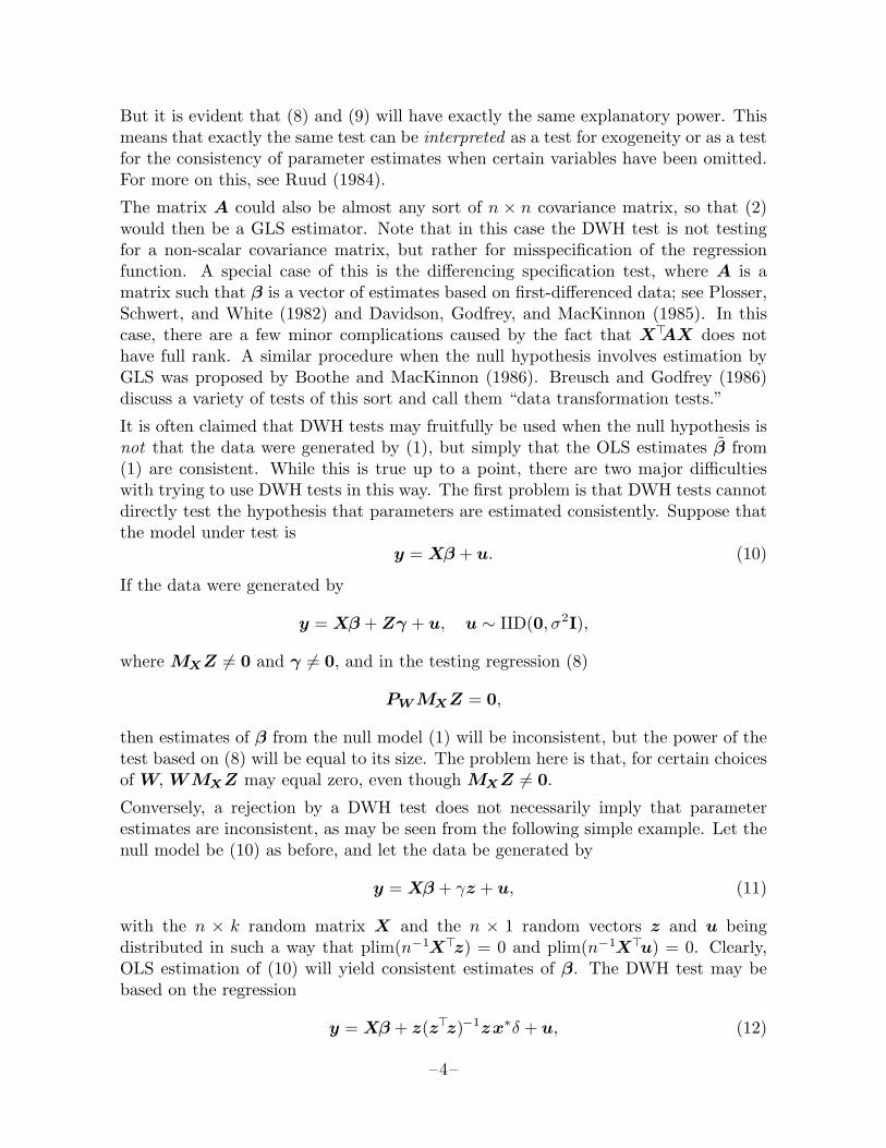
But it is evident that (8) and (9) will have exactly the same explanatory power. Thismeans that exactly the same test can be interpreted as a test for exogeneity or as a testfor the consistency of parameter estimates when certain variables have been omitted.For more on this, see Ruud (1984).

The matrix A could also be almost any sort of n × n covariance matrix, so that (2)would then be a GLS estimator. Note that in this case the DWH test is not testingfor a non-scalar covariance matrix, but rather for misspecification of the regressionfunction. A special case of this is the differencing specification test, where A is amatrix such that β is a vector of estimates based on first-differenced data; see Plosser,Schwert, and White (1982) and Davidson, Godfrey, and MacKinnon (1985). In thiscase, there are a few minor complications caused by the fact that X>AX does nothave full rank. A similar procedure when the null hypothesis involves estimation byGLS was proposed by Boothe and MacKinnon (1986). Breusch and Godfrey (1986)discuss a variety of tests of this sort and call them “data transformation tests.”

It is often claimed that DWH tests may fruitfully be used when the null hypothesis isnot that the data were generated by (1), but simply that the OLS estimates β from(1) are consistent. While this is true up to a point, there are two major difficultieswith trying to use DWH tests in this way. The first problem is that DWH tests cannotdirectly test the hypothesis that parameters are estimated consistently. Suppose thatthe model under test is

y = Xβ + u. (10)

If the data were generated by

y = Xβ + Zγ + u, u ∼ IID(0, σ2I),

where MXZ 6= 0 and γ 6= 0, and in the testing regression (8)

PWMXZ = 0,

then estimates of β from the null model (1) will be inconsistent, but the power of thetest based on (8) will be equal to its size. The problem here is that, for certain choicesof W, WMXZ may equal zero, even though MXZ 6= 0.

Conversely, a rejection by a DWH test does not necessarily imply that parameterestimates are inconsistent, as may be seen from the following simple example. Let thenull model be (10) as before, and let the data be generated by

y = Xβ + γz + u, (11)

with the n × k random matrix X and the n × 1 random vectors z and u beingdistributed in such a way that plim(n−1X>z) = 0 and plim(n−1X>u) = 0. Clearly,OLS estimation of (10) will yield consistent estimates of β. The DWH test may bebased on the regression

y = Xβ + z(z>z)−1zx∗δ + u, (12)

–4–

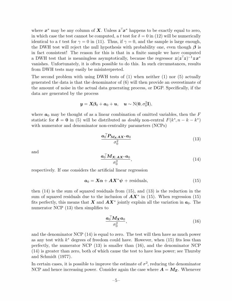
where x∗ may be any column of X. Unless z>x∗ happens to be exactly equal to zero,in which case the test cannot be computed, a t test for δ = 0 in (12) will be numericallyidentical to a t test for γ = 0 in (11). Thus, if γ = 0, and the sample is large enough,the DWH test will reject the null hypothesis with probability one, even though β isin fact consistent! The reason for this is that in a finite sample we have computeda DWH test that is meaningless asymptotically, because the regressor z(z>z)−1zx∗

vanishes. Unfortunately, it is often possible to do this. In such circumstances, resultsfrom DWH tests may easily be misinterpreted.

The second problem with using DWH tests of (1) when neither (1) nor (5) actuallygenerated the data is that the denominator of (6) will then provide an overestimate ofthe amount of noise in the actual data generating process, or DGP. Specifically, if thedata are generated by the process

y = Xβ0 + a0 + u, u ∼ N(0, σ20I),

where a0 may be thought of as a linear combination of omitted variables, then the Fstatistic for δ = 0 in (5) will be distributed as doubly non-central F (k∗, n − k − k∗)with numerator and denominator non-centrality parameters (NCPs)

a0>PMXAX∗a0

σ20

(13)

anda0>MX;AX∗a0

σ20

, (14)

respectively. If one considers the artificial linear regression

a0 = Xα + AX∗ψ + residuals, (15)

then (14) is the sum of squared residuals from (15), and (13) is the reduction in thesum of squared residuals due to the inclusion of AX∗ in (15). When regression (15)fits perfectly, this means that X and AX∗ jointly explain all the variation in a0. Thenumerator NCP (13) then simplifies to

a0>MXa0

σ20

, (16)

and the denominator NCP (14) is equal to zero. The test will then have as much poweras any test with k∗ degrees of freedom could have. However, when (15) fits less thanperfectly, the numerator NCP (13) is smaller than (16), and the denominator NCP(14) is greater than zero, both of which cause the test to have less power; see Thursbyand Schmidt (1977).

In certain cases, it is possible to improve the estimate of σ2, reducing the denominatorNCP and hence increasing power. Consider again the case where A = MZ . Whenever

–5–

ρ(AX) = ρ(MZX) < ρ(Z), the DWH test differs from the classical test for γ = 0 in(7), and the test regression

y = Xβ + MZXδ + u (17)

fits less well than regression (7), because the latter has additional regressors. Insteadof using the ordinary F statistic for δ = 0 in (17), then, one might use the test statistic

y>PMXMZXy/k∗

y>MX;Zy/(n− k − l). (18)

The denominator here is the estimate of σ2 from (7); the ordinary F statistic woulduse the estimate of σ2 from (17).

The test statistic (18) will be asymptotically valid whenever (7) generated the data,and it will have the F (k∗, n − k − l) distribution in finite samples when the nullhypothesis that E(β = β) is true, the regressors are fixed, and the errors are normal.Reducing the number of degrees of freedom in the denominator of an F test has theeffect of reducing power; see Das Gupta and Perlman (1974). Thus, if the data weregenerated by (17), the modified F test (18) would have less power than the ordinaryF test. However, in some cases where (1) is false, (7) may fit much better than (17),thus yielding a much lower estimate of σ2. In such cases, the modified F test (18) willbe more powerful than the ordinary one.

3. General Nonlinear ModelsSince the work of Hausman (1978), it has been well known that DWH tests may beused in the context of very general classes of models involving maximum likelihoodestimation. There are three principal theoretical results in this literature. The first,due to Hausman, is that the (asymptotic) covariance matrix of a vector of contrastsis equal to the difference between the (asymptotic) covariance matrices of the twovectors of parameter estimates, provided that one of the latter is (asymptotically)efficient under the null hypothesis. This is essentially a corollary of the Cramer-Raobound.

The second principal result, due to Holly (1982), is that when the two parametervectors being contrasted correspond to restricted and unrestricted ML estimates (thevectors consisting only of those parameters which are estimated under the restrictions),the DWH test will in certain circumstances be equivalent to the three classical teststatistics, Wald, LM, and LR. Whether this equivalence holds or not will depend onthe numbers of parameters in the restricted and unrestricted models, and on the rankof certain matrices; as we show below, the results are completely analogous to thoseon whether the DWH test based on (17) is equivalent to the F test based on (7).

The third principal result, due to White (1982), Ruud (1984), and Newey (1985), isthat tests asymptotically equivalent to DWH tests can be computed as score tests.As Ruud and Newey recognized, this implies that various artificial regressions can be

–6–

used to compute these tests. The only artificial regression which has been explicitlysuggested for this purpose is the so-called outer-product-of-the-gradient, or OPG, re-gression, in which a vector of ones is regressed on the matrix of contributions fromsingle observations to the gradient of the loglikelihood function. This regression iswidely used for calculating LM tests; see Godfrey and Wickens (1981). It has morerecently been suggested by Newey (1985) as an easy way to calculate “conditional mo-ment” tests, including some which are DWH tests. Unfortunately, the OPG regressionis known to have poor and often disastrous finite-sample properties. See Davidson andMacKinnon (1983, 1985a), Bera and McKenzie (1986), Chesher and Spady (1988), andKennan and Neumann (1988); the last two provide spectacular examples. As we shallnow show, any artificial regression that can be used to compute LM tests can also beused to compute DWH tests. In view of the poor properties of the OPG regression,this result may be important for applied work.

There are many classes of models for which artificial linear regressions other than theOPG regression are available. These include univariate and multivariate nonlinear re-gression models (Engle 1982, 1984), possibly with heteroskedasticity of unknown form(Davidson and MacKinnon, 1985b), probit and logit models (Davidson and MacKin-non, 1984b), and a rather general class of nonlinear models, with nonlinear transfor-mations on the dependent variable(s), for which “double-length” artificial regressionswith 2n “observations” are appropriate (Davidson and MacKinnon, 1984a, 1988). Tothe extent that evidence is available, these all appear to have better finite-sampleproperties than the OPG regression.

We shall deal with the following general case. There is a sample of size n which givesrise to a loglikelihood function

L(θ1, θ2) =n∑

t=1

`(θ1, θ2), (19)

where θ1 is a k --vector and θ2 an l --vector of parameters, the latter equal to zero if themodel is correctly specified. Maximum likelihood estimates of the vector θ = [θ1

>,θ2>]>

under the restriction θ2 = 0 will be denoted θ, while unrestricted estimates will bedenoted θ. The scores with respect to θ1 and θ2 are denoted by g1(θ) and g2(θ); thus

gi(θ) =n∑

t=1

∂`t(θ1, θ2)∂θi

, i = 1, 2.

A hat or a tilde over any quantity indicates that it is evaluated at θ or θ, respectively.

The model represented by (19) is assumed to satisfy all the usual conditions for maxi-mum likelihood estimation and inference to be asymptotically valid; see, for example,Amemiya (1985, Chapter 4). In particular, we assume that the true parameter vectorθ0 is interior to a compact parameter space, and that the information matrix

I(θ) ≡ lim(E(gg>)

)

–7–

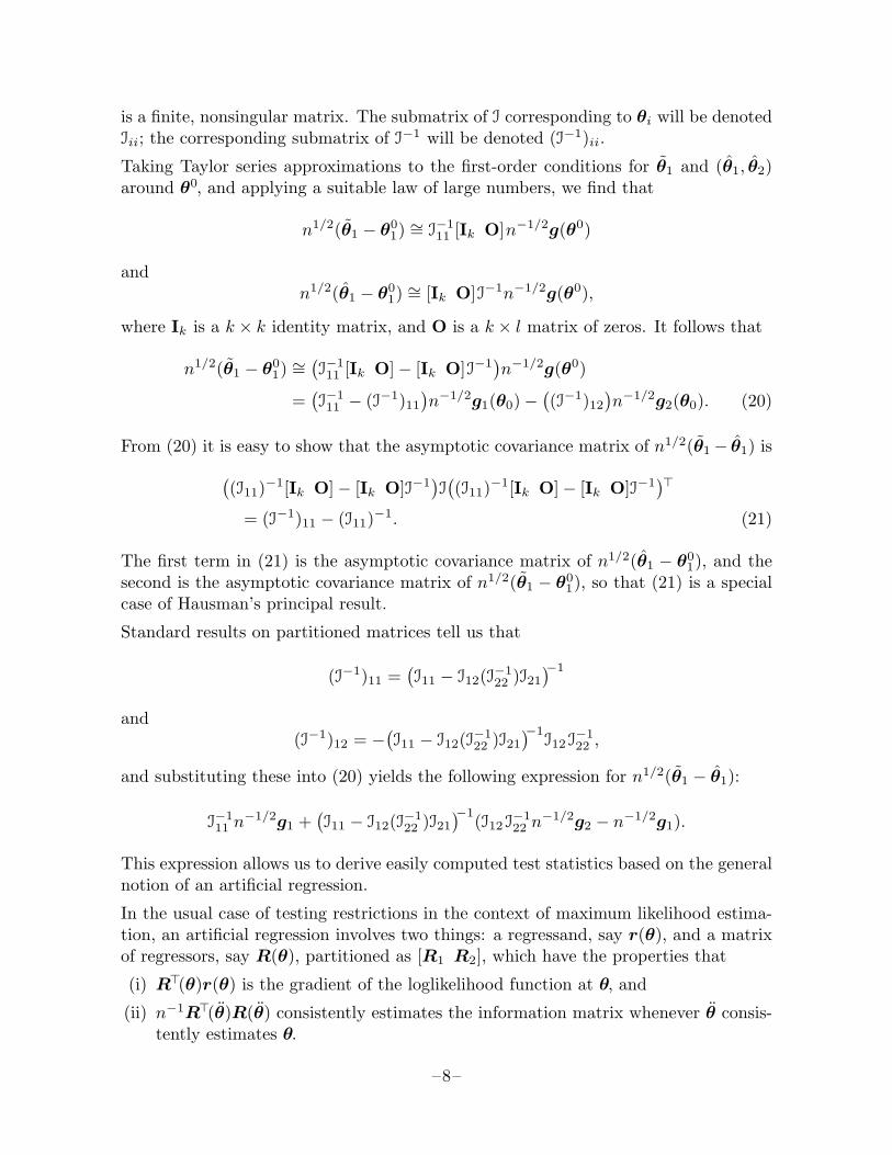
is a finite, nonsingular matrix. The submatrix of I corresponding to θi will be denotedIii; the corresponding submatrix of I−1 will be denoted (I−1)ii.

Taking Taylor series approximations to the first-order conditions for θ1 and (θ1, θ2)around θ0, and applying a suitable law of large numbers, we find that

n1/2(θ1 − θ01) ∼= I−1

11 [Ik O]n−1/2g(θ0)

andn1/2(θ1 − θ0

1) ∼= [Ik O]I−1n−1/2g(θ0),

where Ik is a k × k identity matrix, and O is a k × l matrix of zeros. It follows that

n1/2(θ1 − θ01) ∼=

(I−111 [Ik O]− [Ik O]I−1

)n−1/2g(θ0)

=(I−111 − (I−1)11

)n−1/2g1(θ0)−

((I−1)12

)n−1/2g2(θ0). (20)

From (20) it is easy to show that the asymptotic covariance matrix of n1/2(θ1− θ1) is

((I11)−1[Ik O]− [Ik O]I−1

)I((I11)−1[Ik O]− [Ik O]I−1

)>

= (I−1)11 − (I11)−1. (21)

The first term in (21) is the asymptotic covariance matrix of n1/2(θ1 − θ01), and the

second is the asymptotic covariance matrix of n1/2(θ1 − θ01), so that (21) is a special

case of Hausman’s principal result.

Standard results on partitioned matrices tell us that

(I−1)11 =(I11 − I12(I−1

22 )I21

)−1

and(I−1)12 = −(

I11 − I12(I−122 )I21

)−1I12 I−1

22 ,

and substituting these into (20) yields the following expression for n1/2(θ1 − θ1):

I−111 n−1/2g1 +

(I11 − I12(I−1

22 )I21

)−1(I12 I−122 n−1/2g2 − n−1/2g1).

This expression allows us to derive easily computed test statistics based on the generalnotion of an artificial regression.

In the usual case of testing restrictions in the context of maximum likelihood estima-tion, an artificial regression involves two things: a regressand, say r(θ), and a matrixof regressors, say R(θ), partitioned as [R1 R2], which have the properties that

(i) R>(θ)r(θ) is the gradient of the loglikelihood function at θ, and

(ii) n−1R>(θ)R(θ) consistently estimates the information matrix whenever θ consis-tently estimates θ.

–8–

Replacing the gradients and information sub-matrices in (22) by their finite-sampleanalogues, evaluated at θ, and ignoring factors of n, yields the expression

(R1>R1)−1R1

>r − (R1>M2R1)−1R1

>M2r = −(R1>M2R1)−1R1

>M2M1r, (23)

where Mi denotes the matrix which projects onto the orthogonal complement of thesubspace spanned by the columns of Ri, for i = 1, 2. Notice that the left-hand side of(23) resembles the expression for a restricted OLS estimator minus an unrestricted one.Think of r as the regressand, R1 as the matrix of regressors for the null hypothesis,and M2 as the matrix which projects onto the orthogonal complement of the spacespanned by the additional regressors whose coefficients are zero under the null.

Now consider the artificial regression

r = R1b1 + M2R∗1b2+ residuals, (24)

where the n × k∗ matrix R∗1 consists of as many columns of R1 as possible subject

to the condition that the matrix [R1 M2R∗1] have full rank. The explained sum of

squares from this regression is

r>PR1; M2R∗1r = r>PM1M2R∗1

r,

since R1>r = 0 by the first-order conditions. Under suitable regularity conditions, it is

easily shown that this statistic is asymptotically distributed as χ2(k∗) under the nullhypothesis that θ2 = 0. This result also extends to any situation where the data aregenerated by a sequence of local DGPs with θ2I21 = 0 which tends to θ2 = 0, providedthat I21 has full rank; we discuss this important proviso below.

Notice that (24) may be rewritten as

r = R1(b1 + b2)− R2(R2>R2)−1R2

>R1b2 + residuals.

Thus, as with the linear case, it makes no difference whether we use (24) or

r = R1c1 + P2R∗1c2 + residuals (25)

for the purpose of computing a test.

The classical LM test can of course be computed as the explained sum of squares fromthe artificial regression

r = R1b1 + R2b2 + residuals (26)

The equivalence result of Holly (1982) now follows immediately. Suppose that l < k,so that there are fewer restrictions than parameters under the null hypothesis, andthat R2

>R1 has rank l. Then it must be the case that R1 and

P2R1 = R2(R2>R2)−1R2

>R1

–9–

span the same space as R1 and R2, so that (26) and (25) will have exactly the sameexplanatory power. The LM and DWH tests will then be numerically identical. Pro-vided that I21 = plim(n−1R2

>R1) has full rank l, the asymptotic equivalence of allforms of classical and DWH tests, which is Holly’s result, then follows immediatelyfrom the numerical equality of these two tests.

When I21 does not have full rank, some elements (or linear combinations of elements)of the vector θ1 will be estimated consistently by θ1 even when the restrictions arelocally false. More precisely, if we assume that θ2 = n−1/2η, so that the discrepancybetween θ2 and 0 is O(n−1/2), then when I21 does not have full rank, certain linearcombinations of the components of the vector n1/2(θ1 − θ0

1) will have mean zero,regardless of the value of η. Ordinarily, when I21 has full rank, this could be trueonly for certain values of η (including η = 0), and the DWH test would have powerwhenever η did not have those values. This local result is of course true globally forlinear regression models.

In this situation, the results of DWH tests may easily be misinterpreted. When I21

does not have full rank, one must drop as many columns of P2R1 as necessary andreduce the degrees of freedom for the test accordingly. In practice, however, R2

>R1

may well have full rank even though I21 does not, so that the investigator may notrealize there is a problem. As a result, the null hypothesis of consistency may wellbe rejected even when θ1 is in fact consistent. The key to understanding this is torecognize that, even though the null hypothesis of the DWH version of a classical testis θ2 I21 = 0 rather than θ2 = 0, the test is still testing a hypothesis about θ2 andnot a hypothesis I21. When the test is done by an artificial regression, I21 is merelyestimated by n−1R2

>R1, and if I21 does not have full rank, the estimate by itself willalmost never reveal that fact (although combined with an estimate of the variance ofR2>R1, it could do so). This is precisely analogous to the case of the linear regression

model (10), where incorrectly omitting the regressor Z had no effect on the consistencyof β.

Note that this is a problem for all forms of the DWH test, and not simply for the scoreform. In cases where the information matrix is block-diagonal between the parameterswhich are estimated under the null and the parameters which are restricted, the formerwill always be estimated consistently even when the restrictions are locally false in thesense discussed above. This implies that the asymptotic covariance matrix of the vectorof contrasts, expression (21), must be a zero matrix. But the finite-sample analogueof (21) will almost never be a zero matrix, and it is usually computed in such a wayas to ensure that it is positive semi-definite. As a result, it will be just as possible tocompute, and misinterpret, the DWH statistic in its original form as in its score form.

4. DWH Tests in Other Directions

In Davidson and MacKinnon (1987a), we showed that the Holly result is perfectlygeneral when the null hypothesis is estimated by maximum likelihood. The reasonfor this is that when one set of estimates is asymptotically efficient if the model is

–10–

correctly specified, the other set is always asymptotically equivalent (locally) to MLestimates with some set of restrictions removed; Holly’s result then shows that, whenthe number of restrictions removed is no greater than the number of parameters esti-mated under the null, and the information matrix satisfies certain conditions, a DWHtest is equivalent to a classical test of those restrictions.

As a corollary of this result, we can start with any score-type test and derive a DWHvariant of it, similar to the test based on regression (24). Consider an artificial regres-sion analogous to (26), but with R2 replaced by an n×m matrix Z = Z(θ):

r = R1c1 + Zc2 + residuals. (27)

The matrix Z must satisfy certain conditions, which essentially give it the same prop-erties as R2; these are discussed below. Provided it does so, and assuming that thematrix [R1 Z] has full rank, the explained sum of squares from this regression will beasymptotically distributed as χ2(m) when the DGP is (19) with θ2 = 0.

The variety of tests covered by (27) is very great. In addition to LM tests based on allknown artificial regressions, tests of this form include Newey’s (1985) conditional mo-ment tests, all the score-type DWH tests discussed in sections 2 and 3 above, White’s(1982) information matrix test in the OPG form suggested by Lancaster (1984), andRamsey’s (1969) RESET test.

We now briefly indicate how to prove the above proposition. The proof is similar tostandard proofs for LM tests based on artificial regressions, and the details are thereforeomitted. As noted above, it is necessary that Z satisfy certain conditions, so that itessentially has the same properties as R2. First, we require that plim(n−1r>Z) = 0under the null hypothesis; if this condition were not satisfied, we obviously could notexpect c2 in (27) to be zero. Second, we require that

plim(n−1Z>r>rZ) = plim(n−1Z>Z) (28)

andplim(n−1Z>r>rR1) = plim(n−1Z>R1), (29)

which are similar to the condition that

plim(n−1R1>r>rR1) = plim(n−1R1

>R1); (30)

(30) does not have to be assumed because it is a consequence of property (ii) and theconsistency of θ. Finally, we require that a central limit theorem be applicable to thevector

n−1/2Z>M1r (31)

and that laws of large numbers be applicable to the quantities whose probability limitsappear on the right-hand sides of (28), (29), and (30).

–11–

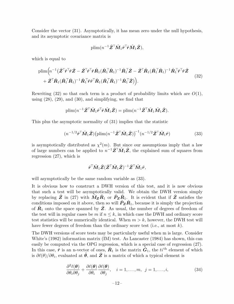
Consider the vector (31). Asymptotically, it has mean zero under the null hypothesis,and its asymptotic covariance matrix is

plim(n−1Z>M1r>rM1Z),

which is equal to

plim(n−1

(Z>r>rZ − Z>r>rR1(R1

>R1)−1R1>Z − Z>R1(R1

>R1)−1R1>r>rZ

+ Z>R1(R1>R1)−1R1

>rr>R1(R1>R1)−1R1

>Z))

.(32)

Rewriting (32) so that each term is a product of probability limits which are O(1),using (28), (29), and (30), and simplifying, we find that

plim(n−1Z>M1r>rM1Z) = plim(n−1Z>M1M1Z).

This plus the asymptotic normality of (31) implies that the statistic

(n−1/2r>M1Z)(plim(n−1Z>M1Z)

)−1(n−1/2Z>M1r) (33)

is asymptotically distributed as χ2(m). But since our assumptions imply that a lawof large numbers can be applied to n−1Z>M1Z, the explained sum of squares fromregression (27), which is

r>M1Z(Z>M1Z)−1Z>M1r,

will asymptotically be the same random variable as (33).

It is obvious how to construct a DWH version of this test, and it is now obviousthat such a test will be asymptotically valid. We obtain the DWH version simplyby replacing Z in (27) with MZR1 or PZR1. It is evident that if Z satisfies theconditions imposed on it above, then so will PZR1, because it is simply the projectionof R1 onto the space spanned by Z. As usual, the number of degrees of freedom ofthe test will in regular cases be m if n ≤ k, in which case the DWH and ordinary scoretest statistics will be numerically identical. When m > k, however, the DWH test willhave fewer degrees of freedom than the ordinary score test (i.e., at most k).

The DWH versions of score tests may be particularly useful when m is large. ConsiderWhite’s (1982) information matrix (IM) test. As Lancaster (1984) has shown, this caneasily be computed via the OPG regression, which is a special case of regression (27).In this case, r is an n-vector of ones, R1 is the matrix G1, the tith element of whichis ∂`(θ)/∂θi, evaluated at θ, and Z is a matrix of which a typical element is

∂2`(θ)∂θi∂θj

+∂`(θ)∂θi

∂`(θ)∂θj

, i = 1, . . . ,m, j = 1, . . . , i, (34)

–12–

evaluated at θ. The number of columns in Z is 12 (k2 + k), although in practice some

columns often have to be dropped if [G1 Z] has less-than-full rank.

Except when k is very small, the IM test is likely to involve a very large number ofdegrees of freedom. Various ways to reduce this have been suggested; one could, forexample, simply restrict attention to the diagonal elements of the information matrix,setting j = i in (34). But this seems arbitrary. Moreover, as Chesher (1984) hasshown, the implicit alternative of the IM test is a form of random parameter variationwhich will not necessarily be of much economic interest. People frequently employ thetest not to check for this type of parameter variation, but because it is thought to havepower against a wide range of types of model misspecification. Model misspecificationis often of little concern if it does not affect parameter estimates. A possible way toreduce the number of degrees of freedom of the IM test, then, is to use a DWH versionof it. This can easily be accomplished by replacing Z in the artificial regression (27)by PZG1.

In many circumstances, we believe, the DWH version of the IM test will be moreuseful than the original. Instead of asking whether there is evidence that the OPGand Hessian estimates of the information matrix differ, the test asks whether there isevidence that they differ for a reason which affects the consistency of the parameterestimates. One could reasonably expect the DWH version of the test to have morepower in many cases, since it will have at most k degrees of freedom, instead of 1

2 (k2+k)for the usual IM test. Note, however, that it will still be impossible to compute thetest when n < 1

2 (k2 + k), since PZG1 would in that case equal G1. Even in its DWHversion, then, the IM test remains a procedure to be used only when the sample sizeis reasonably large.

Of course, it makes sense to do a DWH version of the IM test only when the fulltest is testing in directions which affect parameter consistency. This is by no meansalways so, since the directions in which the IM test tests are those which affect theconsistency of the estimate of the covariance matrix of the parameter estimates. (Andthis implies that even the full IM test will have no power against misspecifications thataffect the consistency of the estimates of neither the parameters nor their covariancematrix.) Consider, for instance, the case of linear regression models, where the IM testis implicitly testing for certain forms of heteroskedasticity, skewness, and kurtosis; seeHall (1987). For a linear regression model with normal errors, the contribution to theloglikelihood function from the tth observation is

`t = 1−2

log(2π)− log(σ)− (yt −Xtβ)2

)/(2σ2) (35)

where β is a p--vector so that k = p+1. The contributions to the gradient for β and σ,respectively, are

Gti(yt −Xtβ)Xti/σ2, (36)

andGtσ = −1/σ + (yt −Xtβ)3/σ2. (37)

–13–

The second derivatives of (35) are

∂2`t

∂σ∂σ= −1/σ2 − 3(yt −Xtβ)2/σ4,

∂2`t

∂σ∂βi= −2(yt −Xtβ)Xti/σ3,

and∂2`t

∂βi∂βj= −XtiXtj/σ2.

The right-hand side of the OPG regression consists of the test regressors Ztj plus pregressors Gti, which correspond to the βi, and one regressor Gtσ, which correspondsto σ (Gti and Gtσ are evaluated at OLS estimates β and σ, the latter using n rathern−p in the denominator). The test regressor corresponding to any pair of parametersis the sum of the second derivative of `t with respect to those parameters and theproduct of the corresponding first derivatives, again evaluated at β and σ.

We simplify all these expressions by using the fact that, since the test statistic is anexplained sum of squares, multiplying any regressor by a constant will have no effecton it, and by defining et as ut/σ. The regressors for the OPG version of the IM testare thus seen to be:

for βi : eiXti, (38)

for σ : e2t − 1, (39)

for βi, βj : (e2t − 1)XtiXtj (40)

for βi, σ : (e3t − 3et)Xti (41)

for σ, σ : e4t − 5e2

t + 2. (42)

When the original regression contains a constant term, (40) will be perfectly collinearwith (39) when i and j both refer to the constant term, so that one of them will haveto be dropped, and the degrees of freedom for the test reduced by one to 1

2 (p2 + 3p).

It is evident that the (βi, βj) regressors are testing in directions which correspond toheteroskedasticity of the type that White’s (1980) test is designed to detect (namely,heteroskedasticity that affects the consistency of the OLS covariance matrix estimator)and that the (βi, σ) regressors are testing in directions that correspond to skewnessinteracting with the Xti. If we subtract (39) from (42), the result is e4

t − 6e2t +3, from

which we see that the linearly independent part of the (σ, σ) regressor is testing inthe kurtosis direction. The IM test is thus seen to be testing for heteroskedasticity,skewness, and kurtosis, none of which prevent β from being consistent. Hence it wouldmake no sense to compute a DWH variant of the IM test in this case, and indeed itwould be impossible to do so asymptotically. If one did do such a test in practice, onewould run into precisely the problem discussed in the previous section: The test mightwell reject if the model suffered from heteroskedasticity, skewness, or kurtosis, but therejection would not say anything about the consistency of β or of σ.

–14–

5. The Power of DWH and Classical TestsWhen the DWH version of a classical test differs from the original, the former may ormay not be more powerful than the latter. Although this fact and the reasons for itare reasonably well-known, it seems worthwhile to include a brief discussion which, wehope, makes the issues clear. We shall deal with the general case of section 3, and wewill rely heavily on results in Davidson and MacKinnon (1987a).

Suppose the data are generated by a sequence of local DGPs which tends to the pointθ0 ≡ (θ0

1,0). The direction in which the null is incorrect can always be representedby a vector

M1(R2w2 + R3w3),

where M1 ≡ M1(θ0), R2 ≡ R2(θ0), and R3 is a matrix with the same properties asR1 and R2, which represents directions other than those contained in the alternativehypothesis. The vectors w2 and w3 indicate the weights to be given to the variousdirections; one can think of w2 as being proportional to θ2. Following Davidson andMacKinnon (1987a), it is possible to show that under such a sequence any of theclassical test statistics for the hypothesis θ2 = 0 will be asymptotically distributed asnoncentral χ2(l) with noncentrality parameter (or NCP)

plim(

1−n(w2

>R2>+ w3

>R3>)M1R2

)(plim

(1−nR2>M1R2

)−1)

× plim(

1−nR2>M1(R2w2 + R3w3

).

(43)

This NCP is the probability limit of n−1 times the explained sum of squares from theartificial regression

M1(R2w2 + R3w3) = M1R2b + residuals. (44)

When the DGP belongs to the alternative hypothesis, so that w3 = 0, this regressionfits perfectly, and (43) simplifies to

plim(

1−nw2>R2

>M1R2w2

),

which is equivalent to expressions for noncentrality parameters found in standard ref-erences such as Engle (1984).

Similarly, the noncentrality parameter for the DWH variant of the classical test againstθ2 = 0 will be the probability limit of n−1 times the explained sum of squares fromthe artificial regression

M1(R2w2 + R3w3) = M1P2R2b∗ + residuals. (45)

If we make the definitionC ≡ (R2

>R2)−1R2>R1,

–15–

regression (45) can be rewritten as

M1(R2w2 + R3w3) = M1R2Cb∗ + residuals. (46)

From (44) and (46), it is clear that the DWH and classical tests will have the sameNCP in two circumstances. The first of these is when l = k and the matrix C hasfull rank, which is the familiar case where the classical and DWH tests are equivalent.The second is when

R2w2 = R2Cw∗, (47)

where w∗ is a k --vector. In both these cases, regressions (44) and (46) will have thesame explained sum of squares.

When the DWH test is not equivalent to the classical tests and condition (47) does nothold, it must have a smaller NCP than the classical tests. This will be true whetheror not w3 = 0, since R2C can never have more explanatory power than R2. Whetherthe DWH test will have more or less power than the classical test then depends onwhether its reduced number of degrees of freedom more than offsets its smaller NCP.

6. Binary Choice Models: An ExampleIn this section, we consider a simple example where a DWH variant of the IM test doesmake sense. Failures of distributional assumptions, of the sort which do not affect theconsistency of least squares estimates, do render ML estimates of binary choice modelsinconsistent. It is therefore both important to test for these and interesting to see ifthey are affecting the parameter estimates.

We shall be concerned with the simplest type of binary choice model, in which thedependent variable yt may be either zero or one and

Pr(yt = 1) = F (Xtβ), (48)

where F (x) is a thrice continuously differentiable function which maps from the realline to the 0–1 interval, is weakly increasing in x, and has the properties

F (x) ≥ 0; F (−∞) = 0; F (∞) = 1; F (−x) = 1− F (x). (49)

Two examples are the probit model, where F (x) is the cumulative standard normaldistribution function, and the logit model, where F (x) is the logistic function. Thecontribution to the loglikelihood of the tth observation is

`t(β) = yt log(F (Xtβ)

)+ (1− yt) log

(F (−Xtβ)

).

The contributions to the gradient for yt = 1 and yt = 0 are, respectively,

f(Xtβ)Xti/F (Xtβ)

–16–

and−f(−Xtβ)Xti/F (−Xtβ),

where f(x) is the first derivative of F (x). Thus the corresponding elements of thematrix G>G are (

f(Xtβ)F (Xtβ)

)2

XtiXtj (50)

and (f(−Xtβ)F (−Xtβ)

)2

XtiXtj . (51)

The second derivatives of `t(β) for yt = 1 and yt = 0 are, respectively,

f ′(Xtβ)F (Xtβ)− f2(Xtβ)F 2(Xtβ)

XtiXtj (52)

and−f ′(Xtβ)F (−Xtβ)− f2(−Xtβ)

F 2(−Xtβ)XtiXtj , (53)

where f ′(x) denotes the derivative of f(x), and we have used the symmetry propertyof (49) which implies that f ′(x) = −f ′(−x). The sum of (50) and (52) is

f ′(Xtβ)F (Xtβ)

XtiXtj , (54)

and the sum of (51) and (53) is

−f ′(Xtβ)F (−Xtβ)

XtiXtj . (55)

The random variable whose two possible realizations are (54) and (55) is the differencebetween the OPG and minus the Hessian. If the model is correctly specified, theexpectation of this random variable is

F (Xtβ)(

f ′(Xtβ)F (Xtβ)

XtiXtj

)+ F (−Xtβ)

(−f ′(Xtβ)F (−Xtβ)

XtiXtj

)

= f ′(Xtβ)XtiXtj − f ′(Xtβ)XtiXtj = 0.

The IM test asks whether it is in fact equal to zero.

The IM test may be based on the OPG regression, as usual, or it may be based on theartificial regression proposed by Engle (1984) and Davidson and MacKinnon (1984b)specifically for binary choice models, which we shall refer to as the PL (for probit andlogit) regression. Computing the IM test by means of an artificial regression otherthan the OPG regression may be attractive because of the very poor finite-sample

–17–

properties of the latter; see Chesher and Spady (1988), Davidson and MacKinnon(1985a), Kennan and Neumann (1988), and Orme (1987b).

The regressand for the PL artificial regression is

rt =yt − F (Xtβ)

(F (−Xtβ)F (Xtβ)

)1/2, (56)

and the regressors corresponding to the βi are

f ′(Xtβ)XtiXtj(F (−Xtβ)F (Xtβ)

)1/2. (57)

We want to construct the test regressors so that the ij th test regressor times (56)yields (54) when yt = 1 and (55) when yt = 0. It is thus easily seen that the ij th testregressor must be

Zt,ij =f ′(Xtβ)XtiXtj(

F (−Xtβ)F (Xtβ))1/2

. (58)

This artificial regression was also derived by Orme (1987a).

In the probit case, this artificial regression has a very interesting interpretation. Sincef(Xtβ) is the standard normal density,

f ′(Xtβ) = −(2π)−1/2 exp(

1−2(Xtβ)2

)Xtβ = −Xtβ f(Xtβ),

so that (58) becomes−f(Xtβ)XtβXtiXtj(F (−Xtβ)F (Xtβ)

)1/2. (59)

This is identical to the test regressor one would get if one did an LM test of the model(48) against the alternative

Pr(yt = 1) = F

((Xtβ)

/exp

( k∑

i=1

i∑

j=1

XtiXtjγij

)), (60)

which can be derived from the latent variable model

y∗t = Xtβ + ut, ut ∼ N(0, exp

(2

k∑

i=1

i∑

j=1

XtiXtjγij

))

yt = 1 if y∗t > 0, yt = 0 otherwise.

(61)

The model (61) is thus a special case of a model which incorporates a natural formof heteroskedasticity. The general model was considered by Davidson and MacKin-non (1984b), who derived the appropriate LM test. This model is special because the

–18–

variance of ut depends exclusively on the cross-products of the Xti. It is clear thatthe implicit alternative of the IM test is precisely this heteroskedastic model. More-over, just as for ordinary regression models it is only heteroskedasticity related to thecross-products of the regressors which affects the consistency of the covariance matrixestimates, so for probit models it is only heteroskedasticity of this type which (locally)prevents the information matrix equality from holding and which thus renders MLprobit estimates inconsistent. This is purely a local result, of course; if a DGP involv-ing any form of heteroskedasticity were some fixed distance from the probit model,one could not expect ML estimates based on homoskedasticity to be consistent.

Notice that if one of the Xti, say Xtj , is a constant term, the test regressor (59) whichcorresponds to Xtj is

−f(Xtβ)Xtβ(F (Xtβ)F (−Xtβ)

)1/2,

which is a linear combination of the regressors (57) that correspond to the βi. This testregressor must therefore be dropped, and the degrees of freedom of the test reducedto 1

2k(k + 1)− 1.

Newey (1985) recognized that the IM test implicitly tests against heteroskedasticity inthe case of probit models, and he suggested that this test may be particularly attractivefor such models. He proposed to use the OPG form of the test. The PL version dis-cussed here is no more difficult to compute than the OPG form, however, and it seemsto have much better finite-sample properties. In the Appendix, we present detailedresults of a small Monte Carlo experiment designed to investigate the performance ofthe OPG and PL tests, in regular and DWH versions.

The Monte Carlo experiments yielded two main results. First, we found that thePL form of the IM test proposed above performed reasonably well for moderatelylarge samples, but that it generated far too many realizations in the right-hand tail,and that its rate of convergence to its asymptotic distribution was disappointinglyslow. (Since binary choice models are often estimated with large samples, this will notnecessarily be a fatal drawback.) In contrast, the OPG form of the IM test performeddismally in samples of all sizes, sometimes rejecting the null more than 90% of thetime at the nominal 5% level. These dreadful results are consistent with those ofChesher and Spady (1988), Davidson and MacKinnon (1985a), Kennan and Neumann(1988), and Orme (1987) for other applications of the OPG form of the IM test; theproblem is primarily that n−1G>G tends to estimate I(θ) very poorly. Like Kennanand Neumann, we found that the performance of the OPG form deteriorated markedlyas the number of degrees of freedom for the test was increased.

Second, we found that in some realistic cases, but not all cases, the DWH version of theIM test can have significantly more power than the ordinary version. This was mostlikely to be the case when the number of parameters was large, so that the DWH variantof the IM test would have many fewer degrees of freedom than the ordinary IM test;unfortunately, this was also the circumstance in which the finite-sample performanceof all the tests was worst.

–19–

Based on these results, we find it difficult to endorse Newey’s (1985) recommendation ofthe IM test for probit models. The conventional OPG form of the test should clearlynot be used. Among the tests we studied, the DWH version computed via the PLregression generally performs the best, both under the null and under the alternativeswe studied, but its finite-sample performance is far from ideal. It might well be moreproductive to test for particular, relatively simple forms of heteroskedasticity whichdo not involve many degrees of freedom, especially those which seem plausible for themodel at hand, rather than to calculate any form of the IM test.

7. ConclusionThis paper has dealt with several aspects of Durbin-Wu-Hausman tests. The maincontribution of the paper has been to show that DWH tests may be based on anyartificial regression that can be used to compute score-type tests, and that any testbased on such a regression can be converted into a DWH test. In particular, we haveshown that this is true for the information matrix test, and we have demonstrated howto compute a DWH version of the IM test for the case of binary choice models.

References

Amemiya, T. (1985). Advanced Econometrics, Cambridge, MA, Harvard UniversityPress.

Bera, A. K., and C. R. McKenzie (1986). “Alternative forms and properties of thescore test,” Journal of Applied Statistics, 13, 13–25.

Boothe, P., and J. G. MacKinnon (1986). “A specification test for models estimatedby GLS,” Review of Economics and Statistics, 68, 711–714.

Breusch, T. S., and L. G. Godfrey (1986). “Data transformation tests,” EconomicJournal, 96, 47–58.

Chesher, A. (1984). “Testing for neglected heterogeneity,” Econometrica, 52,865–872.

Chesher, A., and R. Spady (1988). “Asymptotic expansions of the informationmatrix test statistic,” presented at the Econometric Study Group meeting,Bristol.

Das Gupta, S., and M. D. Perlman (1974). “Power of the noncentral F test: Effectof additional variates on Hotelling’s τ2 test,” Journal of the American StatisticalAssociation, 69, 174–180.

Davidson, R., L. G. Godfrey, and J. G. MacKinnon (1985). “A simplified version ofthe differencing test,” International Economic Review, 26, 639–647.

Davidson, R., and J. G. MacKinnon (1983). “Small sample properties of alternativeforms of the Lagrange Multiplier test,” Economics Letters 12, 269–275.

–20–

Davidson, R., and J. G. MacKinnon (1984a). “Model specification tests based onartificial linear regressions, International Economic Review, 25, 485–502.

Davidson, R., and J. G. MacKinnon (1984b). “Convenient specification tests forlogit and probit models,” Journal of Econometrics, 25, 241–262.

Davidson, R., and J. G. MacKinnon (1985a). “Testing linear and loglinearregressions against Box-Cox alternatives,” Canadian Journal of Economics, 25,499–517.

Davidson, R., and J. G. MacKinnon (1985b). “Heteroskedasticity-robust tests inregression directions. Annales de l’INSEE, 59/60, 183–218.

Davidson, R., and J. G. MacKinnon (1987a). “Implicit alternatives and the localpower of test statistics. Econometrica, 55, 1305–1329.

Davidson, R., and J. G. MacKinnon (1988). “Double-length artificial regressions.Oxford Bulletin of Economics and Statistics, 50, 203–217.

Durbin, J. (1954). “Errors in variables,” Review of the International StatisticalInstitute, 22, 23–32.

Engle, R. F. (1982). “A general approach to Lagrange multiplier model diagnostics,Journal of Econometrics, 20, 83–104.

Engle, R. F. (1984). “Wald, likelihood ratio and Lagrange multiplier testsin econometrics,” in Z. Griliches and M. Intriligator (ed.), Handbook ofEconometrics, Amsterdam, North Holland.

Fisher, G. R., and R. J. Smith (1985). “Least squares theory and the Hausmanspecification test,” Queen’s University Economics Working Paper No. 641.

Godfrey, L. G., and M. R. Wickens (1981). “Testing linear and log-linear regressionsfor functional form,” Review of Economic Studies, 48, 487–496.

Hall, A. (1987). “The information matrix test for the linear model,” Review ofEconomic Studies, 54, 257–263.

Hausman, J. A. (1978). “Specification tests in econometrics,” Econometrica, 46,1251–1272.

Holly, A. (1982). “A remark on Hausman’s specification test. Econometrica, 50,749–759.

Kennan, J., and G. R. Neumann (1988). “Why does the information matrixtest reject too often? A diagnosis of some Monte Carlo symptoms,” HooverInstitution, Stanford University, Working Papers in Economics E-88-10.

Lancaster, T. (1984). “The covariance matrix of the information matrix test,”Econometrica, 52, 1051–1053.

–21–

Nakamura, A., and M. Nakamura (1981). “On the relationships among severalspecification error tests presented by Durbin, Wu and Hausman. Econometrica,49, 1583–1588.

Newey, W. K. (1985). “Maximum likelihood specification testing and conditionalmoment tests,” Econometrica, 53, 1047–1070.

Orme, C. (1987a). “The calculation of the information matrix test for binary datamodels,” University of York, mimeo.

Orme, C. (1987b). “The small sample performance of the information matrix test,”University of York, mimeo.

Plosser, C. I., G. W. Schwert, and H. White (1982). “Differencing as a test ofspecification,” International Economic Review, 23, 535–552.

Ramsey, J. B. (1969). “Tests for specification errors in classical linear least-squaresregression analysis,” Journal of the Royal Statistical Society, Series B, 31,350–371.

Ruud, P. A. (1984). “Tests of specification in econometrics. Econometric Reviews, 3,211–242.

Thursby, J. G., and P. Schmidt (1977). “Some properties of tests for specificationerror in a linear regression model,” Journal of the American StatisticalAssociation 72, 635–641.

White, H. (1980). “A heteroskedasticity-consistent covariance matrix estimator anda direct test for heteroskedasticity,” Econometrica, 48, 817–838.

White, H. (1982). “Maximum likelihood estimation of misspecified models,”Econometrica, 50, 1-25.

Wu, D. (1973). “Alternative tests of independence between stochastic regressors anddisturbances,” Econometrica, 41, 733–750.

–22–

Appendix

In this appendix, we report the results of a small Monte Carlo experiment designed toshed light on Newey’s (1985) conjecture that the IM test may be particularly attractivefor probit models. There are two main results. First, we find that the OPG form of theIM test for probit models rejects the null far too often in samples of moderate or evenrather large size, while the PL form of the IM test proposed in this paper performsmuch better. Second, we find that in some realistic cases the DH version of the IMtest may have significantly more power than the ordinary version.

In all our experiments, the matrix X consisted of a constant term and one or moreother regressors, which were normally distributed and equi-correlated with correlationone half. Only one set of realizations of these variables was generated, and only for 100observations. For larger sample sizes, this set of observations was replicated as manytimes as necessary. This scheme reduced the costs of the simulation, made it easy tocalculate NCPs (which for a given test depend only on X and on the parameters ofthe DGP), and ensured that any changes as n was increased were not due to changesin the pattern of the exogenous variables.

We first investigated the performance under the null of the ordinary IM test and itsDH version, calculated by both the OPG and PL regressions, for samples of size 100,200, 400, 800, and 1600. We let k, the number of parameters under the null hypothesis,vary from 2 to 4, so that the number of degrees of freedom for the ordinary IM testwas 2, 5, or 9, and for the DH version 2, 3, or 4. The DH and ordinary IM tests arethus identical when k = 2.

Results for samples of sizes 100, 400, and 1600 are shown in Table 1. The most strikingresult is the extreme tendency to over-reject of the OPG tests, which worsens rapidlyas k increases and diminishes only slowly as the sample size increases. For k = 4, theOPG IM test rejects over 98% of the time at the nominal 5% level when n = 100,and over 50% of the time even when n = 1600. It is clear that the sample wouldhave to be enormous for this test’s true size to be anywhere close to its nominal one.The DH version of the OPG test is slightly better behaved than the original, but theimprovement is marginal. Previous results on the finite-sample performance of theOPG test have generally not been favorable to it, but the present results are far worsethan those reported previously. Since most applications are likely to involve manymore than four parameters, it seems doubtful that the OPG form of the IM test forprobit models can ever yield even approximately reliable results in samples of the sizethat are typically used by econometricians.

The tests based on the PL regression are far better behaved than the OPG tests, butare still a long way from their asymptotic distribution even in samples of 1600. Theyhave roughly the right mean, but their standard deviations are too high because verylarge values occur much more often than they should by chance. As a result, theytend to under-reject at the 10% level and over-reject at the 1% level, while being fairlyclose to their nominal size at 5%. Curiously, the problem of too many outliers appearsinitially to get worse as n increases; for k = 4 (the worst case), the standard deviation

–23–

for both the ordinary and DH versions is largest for n = 400, as is the rejectionfrequency at the nominal 1% level.

Since the OPG test rejects so often as to be completely useless, there is apparently nochoice but to use the PL version; however, these results suggest that even it shouldbe regarded with considerable suspicion, especially if there are more than a very fewparameters and the sample size is not very large indeed.

Our second set of experiments was designed to investigate power when the data weregenerated by (61). Calculation of NCPs showed that, for a wide range of γij chosenso that all cross-products contributed very roughly the same amount to the variance,the NCP for the DH version was only slightly smaller than the NCP for the ordinaryIM test. In more extreme cases, such as when only one γij was non-zero, the NCP forthe DH version could be less than half as large. In the former case, the DH versionshould be more powerful asymptotically, since a slight reduction in the NCP is morethan offset by what can be a substantial reduction in degrees of freedom, but in thelatter the ordinary IM test would be more powerful.

The object of the Monte Carlo experiments was to see how accurately the asymptoticanalysis of Section 5 predicted finite-sample power. We considered a single “plausible”pattern for the γij and then scaled the latter to the sample size so that the tests wouldhave power somewhere around 50% at the nominal 5% level. The resulting NCPs,which are of course invariant to the sample size, were 5.15 for k = 2, 6.18 and 5.97(DH version) for k = 3, and 9.16 and 8.57 (DH version) for k = 4.

Results for the PL tests only are shown in Table 2; results for the OPG tests are notshown because, as one would expect from the results in Table 1, they always rejectedfar more often than asymptotic theory predicted. The table also shows, in rows labelled“Asymp”, the values that would be expected if the test statistics actually had theirasymptotic non-central chi-squared distributions.

The behavior of the PL tests when the null is false is broadly consistent with theirbehavior when it is true. In particular, they reject much too often at the 1% level, andthey have means which are often far too large, because there are many more extremelylarge values than asymptotic theory predicts. However, they do not consistently under-reject at the 10% level, and the pattern as n increases is not always monotonic. Forthe case considered here, asymptotic analysis predicts that the DH version will have amodest power advantage. This is usually the case in the experimental results as well,although the ordinary IM test is sometimes more powerful when n is small, especiallyat the 1% level.

–24–

Table 1. Performance of Alternative Tests Under the Null

k Obs. Test Mean Std. Dev. Rej. 10% Rej. 5% Rej. 1%

2 100 OPG 6.94∗∗ 7.36∗∗ 46.5∗∗ 40.1∗∗ 28.2∗∗

PL 1.81∗ 2.67∗∗ 7.8∗ 5.2 2.3∗∗

2 400 OPG 4.11∗∗ 5.45∗∗ 28.0∗∗ 21.4∗∗ 12.4∗∗

PL 1.91 2.04 8.2∗ 4.1 1.2

2 1600 OPG 2.74∗∗ 3.60∗∗ 17.3∗∗ 11.0∗∗ 4.9∗∗

PL 1.96 1.95 9.3 4.3 1.0

3 100 OPG 21.71∗∗ 11.27∗∗ 84.5∗∗ 79.5∗∗ 67.6∗∗

PL 4.14∗∗ 5.87∗∗ 6.6∗∗ 4.9 2.7∗∗

OPG-DH 15.79∗∗ 11.07∗∗ 76.7∗∗ 70.1∗∗ 57.5∗∗

PL-DH 2.44∗∗ 4.69∗∗ 6.0∗∗ 4.4 2.3∗∗

3 400 OPG 13.40∗∗ 10.82∗∗ 55.7∗∗ 47.5∗∗ 32.2∗∗

PL 4.79 4.87∗∗ 9.8 6.4∗ 3.1∗∗

OPG-DH 9.31∗∗ 9.09∗∗ 51.2∗∗ 44.0∗∗ 30.3∗∗

PL-DH 2.81∗ 3.51∗∗ 8.8 5.7 2.4∗∗

3 1600 OPG 8.53∗∗ 6.94∗∗ 33.6∗∗ 25.3∗∗ 14.2∗∗

PL 4.91 4.04∗∗ 9.7 6.2∗ 2.9∗∗

OPG-DH 5.55∗∗ 5.81∗∗ 29.3∗∗ 22.9∗∗ 12.7∗∗

PL-DH 2.95 3.21∗∗ 9.6 5.8 2.4∗∗

4 100 OPG 35.37∗∗ 8.70∗∗ 99.4∗∗ 98.3∗∗ 94.2∗∗

PL 6.64∗∗ 5.72∗∗ 6.2∗∗ 4.5 2.6∗∗

OPG-DH 22.09∗∗ 10.01∗∗ 92.0∗∗ 88.7∗∗ 79.4∗∗

PL-DH 2.60∗∗ 3.19∗∗ 4.8∗∗ 3.0∗∗ 1.6∗

4 400 OPG 37.48∗∗ 21.15∗∗ 88.9∗∗ 84.4∗∗ 75.2∗∗

PL 8.22∗∗ 7.92∗∗ 9.1 6.6∗ 3.7∗∗

OPG-DH 24.72∗∗ 19.82∗∗ 82.0∗∗ 75.8∗∗ 65.4∗∗

PL-DH 3.57∗∗ 5.17∗∗ 8.0∗ 5.6 2.8∗∗

4 1600 OPG 21.94∗∗ 15.81∗∗ 62.5∗∗ 53.1∗∗ 38.5∗∗

PL 8.78 5.51∗∗ 9.9 6.0∗ 2.6∗∗

OPG-DH 12.92∗∗ 13.35∗∗ 55.7∗∗ 47.3∗∗ 33.3∗∗

PL-DH 3.76∗ 3.63∗∗ 8.9 5.8 2.2∗∗

All results are based on 2000 replications.∗ and ∗∗ indicate that a quantity differs from what it should be asymptotically at the .05 and.001 levels, respectively.

Degrees of freedom for the ordinary IM tests are 2 for k = 2, 5 for k = 3, and 9 for k = 4.

The standard deviations of χ2 random variables with 2, 3, 4, 5, and 9 degrees of freedom are,respectively, 2, 2.45, 2.83, 3.16, and 4.24.

–25–

Table 2. Power of Alternative Tests

k Obs. Test Mean Rej. 10% Rej. 5% Rej. 1%

2 Asymp. PL 7.15 64.0 51.6 28.3

100 PL 7.40 47.4∗∗ 40.3∗∗ 27.1∗

200 PL 7.49∗ 53.6∗∗ 44.0∗∗ 27.7

400 PL 7.77∗∗ 59.5∗∗ 48.9* 30.0

800 PL 7.90∗∗ 62.1 51.0 30.1

1600 PL 7.76∗∗ 65.4 53.2 31.4∗

3 Asymp. PL 11.18 57.4 44.5 22.6

PL-DH 8.97 64.0 51.5 28.5

100 PL 35.19∗∗ 55.1∗ 52.1∗∗ 46.8∗∗

PL-DH 31.43∗∗ 57.2∗∗ 51.5 44.9∗∗

200 PL 37.29∗∗ 63.2∗∗ 58.4∗∗ 51.6∗∗

PL-DH 33.02∗∗ 65.5 58.8∗∗ 49.0∗∗

400 PL 30.76 61.3∗∗ 56.4∗∗ 48.9∗∗

PL-DH 26.62∗∗ 64.9 57.5∗∗ 47.2∗∗

800 PL 23.22∗∗ 65.2∗∗ 58.5∗∗ 47.8∗∗

PL-DH 19.27∗∗ 67.2∗ 60.4∗∗ 46.3∗∗

1600 PL 17.84∗∗ 64.6∗ 56.5∗∗ 42.0∗∗

PL-DH 14.47∗∗ 67.1∗ 58.1∗∗ 43.1∗∗

4 Asymp. PL 18.16 64.5 51.9 28.6

PL-DH 12.57 75.0 63.9 40.1

100 PL 114.08∗∗ 50.8∗∗ 48.9∗ 45.9∗∗

PL-DH 114.18∗∗ 51.7∗∗ 50.1∗∗ 47.3∗∗

200 PL 159.94∗∗ 67.0∗ 64.3∗∗ 59.6∗∗

PL-DH 141.66∗∗ 69.8∗∗ 66.2∗ 61.0∗∗

400 PL 120.85∗∗ 68.7∗∗ 64.1∗∗ 57.8∗∗

PL-DH 107.29∗∗ 73.0∗ 68.8∗∗ 61.1∗∗

800 PL 69.29∗∗ 66.0 61.2∗∗ 51.4∗∗

PL-DH 60.12∗∗ 72.6∗ 67.2∗ 56.9∗∗

1600 PL 33.78∗∗ 60.0∗∗ 53.4 40.5∗∗

PL-DH 27.15∗∗ 68.5∗∗ 60.6∗ 48.6∗∗

All results are based on 2000 replications.∗ and ∗∗ indicate that a quantity differs from what it should be asymptotically at the .05 and.001 levels, respectively.

Degrees of freedom for the ordinary IM tests are 2 for k = 2, 5 for k = 3, and 9 for k = 4.

–26–