Testing for Competition in the South AfricanBanking Sector�y

January 29, 2013

Abstract

This paper uses panel data on banks to determine the level of com-

petition in the South African banking sector. Unlike earlier studies

such as Claessens and Laeven (2004), and Bikker et al. (2012) who test

for competition in the South African banking sector using the Panzar-

Rosse methodology, we employ both the Panzar and Rosse (1987) and

the Bresnahan (1982) models to test for the conduct of South African

banks during the periods 1998 to 2008 and 1992 to 2008 for the Pan-

zar and Rosse and Bresnahan models respectively. We �nd evidence

consistent with monopolistic competition in the South African bank-

ing sector. While this may be considered relatively good news from

the consumers�and authorities�viewpoints (South African banks are

not acting as a cartel) given the high concentration, there is need for

policies and other interventions to bring about more contestability in

the banking sector and thus improve e¢ ciencies. In addition, there

is need for continued vigilance by authorities to prevent banks from

cartelising.

Jelclassi�cation: C33, D4, G21, L1

�We thank the Editor and two anonymous referees for valuable comments and sugges-tions. We also thank Profs. Martin Wittenberg and Steve Koch for useful suggestions.We also thank Economic Research Southern Africa (ERSA) and the Competition Com-mission of South Africa for �nancial support. All the remaining errors are the authors�responsibility.

yThe views expressed herein are solely those of the authors - they do not re�ect theviews of the authors�respective institutions.

1

Key words: banking industry, competition, South Africa, Panzar-Rossemodel, Bresnahan model

1 Introduction

A competitive banking sector is important for the proper functioning of the

economy. Indeed, the banking sector is the cornerstone of any properly func-

tioning modern economy. At a micro level, banks, just like any other �rms,

sell products to consumers - hence we need to worry about e¢ ciency impli-

cations if the banking sector is not competitive. However, banks are much

more important than this at a macro level. Firstly, banks advance credit or

loans to both �rms and consumers and thus an uncompetitive banking sector

may lead to an underprovision of such credit or loans (Claessens & Laeven,

2005). This may negatively impact the overall economic performance of the

country. Secondly, banks act as the primary conduit of monetary policy. In

this regard, a low level of competition in the banking sector may hamper the

e¤ectiveness of monetary policy as banks may not respond appropriately to

monetary tightening and/or easing (Van Leuvensteijn et al. 2008).1

It is for these and other reasons that the issue of determining the level of

competition in the banking sector should be a topic of interest to academics,

policy makers as well as the general public. Despite the importance of such

competition research however, there has historically been very few studies

of the level of competition in the African banking sector in general and the

South African banking sector in particular. The South African economy

is the largest economy in Africa, constituting about 19% of Africa�s GDP

(Grobbelaar, 2004). Similarly, South Africa�s banking sector is the most

developed on the continent, and South Africa�s big four banks (ABSA, First

National Bank (FNB), Standard Bank and Nedbank) have branches in many

African countries, especially in the Southern African Development Commu-

nity (SADC). While data issues constrain conduct studies of the African

1 Indeed, Kot (2004), in his study of the interest rate pass-through in the new EU-member states, �nds that increases in the degree of competition in the banking sectorcoincides with faster transmission of the monetary policy impulses to the consumer creditprices.

2

banking sector as a whole, there is fairly good data available for the South

African banking sector - hence this study will focus on the South African

banking sector.

Looking at prior structural studies of the South African banking sector,

authors such as Falkena et al. (2004) and Okeahalam (2001) have gener-

ally concluded that the sector is highly concentrated. This high level of

concentration is due to a few large banks dominating the market. High con-

centration on its own however does not imply lack of competition.2 There

is therefore a need to �test�for competition in order to understand the con-

duct of the banks. This paper is an attempt at a comprehensive study of

the nature of competition in the South African banking sector.

Many authors3 have given much criticism to using structural methods

when measuring competition in the banking sector. First, there is no one-

way causal relationship between structure and conduct as purported by the

SCP literature. As Demsetz (1973) shows, conduct itself can determine

structure. Thus both conduct and structure should be treated as endoge-

nous. Second, high concentration does not imply lack of competition, as the

textbook Bertrand model with homogenous products would attest to. Third,

the link between structure and performance is tenuous at best.4 This paper

therefore focuses on non-structural forms of measurement which takes into

account that banks behave di¤erently depending on the market structure in

which they operate (Baumol, 1982).

The non-structural models used are the Panzar and Rosse (1987) model

and the Bresnahan (1982) model. Our results from these two models sug-

gest that the South African banking sector is monopolistic competition in

nature - consistent with the �nding from Bikker et al. (2012) who only use

the Panzar-Rosse methodology.5 While this may be viewed as �good�news

2 Indeed in the textbook model, under certain conditions, perfect competi-tion/contestability is achieved with only two �rms in the market (see for instance Tirole(1987), Baumol et al. (1982)).

3 Including Demsetz (1973); Berger (1995); and Mullineux & Sinclair (2000).4See section 3 for an indepth discussion.5Studies that estimate scaled revenue equations such as Claessens & Laeven (2004)

tend to �nd much higher levels of competition in the South African banking sector � aresult of the upward bias in these models.

3

by authorities, and to a lesser extent consumers (South African banks are

not acting as a cartel), this �nding suggests a need for policies and other in-

terventions to bring about more contestability in the banking sector. These

could include for example policies and measures that lower switching costs

for consumers or lock-ins. In addition, given the dominance of the four

largest banks, the scope for collusion is a risk that should be managed �

hence policy makers and sector regulators should remain vigilant.

This paper is organised as follows: Section 2 provides context to the

study, highlighting relevance of study beyond South African borders. Sec-

tion 3 discusses the various theories and methods used to measure compe-

tition and gives an overview of the South African banking sector. Section 4

discusses the Panzar and Rosse approach in detail while section 5 provides

the analysis and results of the Bresnahan methodology. Section 6 makes

a comparison of the results of this paper to outcomes found in comparable

developing countries and section 7 concludes the paper.

2 South Africa in Africa - broader relevance of study

As alluded to above, the present study will seek to determine the compet-

itiveness of the South African banking sector. We argue nonetheless that

the study has broader relevance for Africa, given South Africa�s economic

position and role in Africa. First, South Africa is the largest economy in the

whole of Africa, contributing about 19% to the continent�s GDP (Grobbe-

laar, 2004), and about 30% to Sub-Saharan Africa�s GDP (World Bank,

2011). Developments in South Africa therefore matter, especially given in-

creasing economic ties on the continent.

Second, since 1994 South African �rms have intensi�ed their invest-

ment into the continent, thus strengthening economic ties between South

Africa and the rest of the continent. For example, South African �rms

like MTN, Vodacom, SABMiller and Mvelaphanda Holdings are increasingly

showing their presence in Africa (Grobbelaar, 2004; Ramjee and Gwatidzo,

2012). Also, the country�s major banks, ABSA, FNB, Nedbank and Stan-

dard Bank do not only dominate the banking sectors in South Africa and the

4

other South African Customs Union (SACU) members (Botswana, Namibia,

Lesotho and Swaziland), they are also increasingly expanding their opera-

tions in other African countries, either through alliances with local banks or

on their own banners. For example Standard Bank, through its own opera-

tions and through Stanbic, has operations in 17 African countries. Nedbank,

by joining forces with Ecobank with operations in 32 African countries, also

has a huge presence on the continent. Through Barclays,6 ABSA now has

operations in 12 African countries, while FNB has operations in 6 African

countries (Table 1).

Table 1 about here.

Finally, South Africa is not only the only African country in the Group

of 20 (G-20) countries, where issues around �nance and the �nancial sector

are discussed, but it also recently joined the BRICS (Brazil, Russia, India,

China and South Africa ) countries, something which may further enhance

South Africa�s role as the gateway to Africa; further enhancing trade and

investment into the rest of Africa.

As alluded to earlier, an e¢ cient and competitive banking sector is im-

portant for growth (Claessens & Laeven, 2005) - hence the need for studies

that examine the competitiveness of the banking sector in Africa. Data de�-

ciency in a number of African countries however implies that an investigation

of the competitiveness of the banking sectors in the whole of Africa is not

feasible at present. Consequently, we focus on South Africa, but the study

has broader relevance given the importance of the South African banking

sector in Africa.

3 Literature Review

3.1 Banking Competition Theory

There have traditionally been two main methods for determining the level

of competition in the banking sector, namely tests on structural and non-

structural characteristics of banks.6Barclays acquired ABSA in 2005.

5

The structural tests focus on characteristics such as the level of concen-

tration in the industry, the number of banks, market share, etc. (Bain, 1951).

There are two main structural theories, the structure-conduct-performance

(SCP) framework and the e¢ ciency hypothesis (EH) (Bikker & Haaf, 2001).

The SCP framework says that in highly concentrated markets, banks use

market power to increase pro�ts through higher loan prices and lower de-

posits rates - leading to a low level of competition (Bain, 1951). This is a

commonly used structural test for competition.

There are many criticisms to the SCP framework. One theoretical criti-

cism was originally put forth by Demsetz (1973) and later by Berger (1995).

They postulate that, contrary to the SCP approach, the larger market shares

which lead to a high level of concentration, are a result of better e¢ ciency

and lower costs rather than a low level of competition. Other arguments

against the use of concentration as a measure of the level of competition

includes the theory introduced by Mullineux & Sinclair (2000). They ar-

gue that although higher concentration may lead to higher prices, and as

a result lower demand, it does not necessarily result in higher pro�ts for

a highly concentrated banking sector. Indeed, the modern (New Empirical

Industrial Organization (NEIO)) view is that both industry structure and

industry performance are endogenous - being driven by some other factors.

As Schmalensee (1989) puts it, �...except in textbook competitive markets,

derived market structure is clearly a¤ected by market conduct in the long

run�(p. 954). The NEIO thus does not assume a causal relationship be-

tween market structure and performance, but rather, the approach tests

competition and the use of market power (Bikker & Haaf, 2002: 21; Bres-

nahan, 1989).

The most commonly used non-structural models in banking sector stud-

ies are the Panzar and Rosse approach (Rosse & Panzar, 1977; Panzar &

Rosse, 1987) and the Bresnahan model7 (Bresnahan, 1982).8 These models

7Added to by Lau (1982).8The third model, the Iwata model (Iwata, 1974), is less utilised due to its rigid data

requirements (Perera et al. 2006). The Bresnahan model is an improved version of theIwata model and has been used in numerous studies.

6

recognise that banks behave di¤erently depending on the market structures

in which they operate (Baumol, 1982). They also do not ignore the relation-

ship between market contestability and revenue behaviour at the �rm level,

which the structural methods do (Perera et al. 2006).

3.2 Overview of the South African Banking Sector

In the recent Banking Enquiry carried out by the Enquiry Panel of the

Competition Commission (Jali et al. 2008), it was concluded that the South

African banks were not acting as a cartel.9 Despite this, the panel also

believes that the cost and trouble involved for customers to switch banks

weakens the competitive e¤ect of price di¤erences between banks. They

stated that this �allows supra-competitive pricing to be maintained.� (Jali

et al. 2008. p.28). The Competition Commission�s Enquiry Panel therefore

suggests that although there is competition in the banking sector, there is

still need for intervention in certain aspects of the banks�conduct. They rec-

ommend that banks should have to ensure greater transparency and disclose

product and pricing information; reduce search costs and improve compara-

bility between products; and reduce the actual cost of switching and assist

consumers in doing so. This would result in greater ease for customers to

switch between banks and prevent them from being locked in once they have

joined a bank. The panel believes that this will in turn raise the level of

competition in the banking sector. There is no guarantee of this improve-

ment in competition though. Increasing the market transparency on the

products and prices o¤ered by banks may actually help facilitate collusion

in the market (See for instance Tirole, 1988).10

Table 2 below shows how important the South African banking sector is

9This conclusion is arrived at based on qualitative (as opposed to quantitative) analysesof the banking sector.10A case where increased market transparency was harmful to competition is the famous

case in Danish Cement industry whereby the competition authority decided to interveneto enhance the competition by requiring a daily price list (for two grades of ready-mixedconcrete) to be revealed but this had an adverse e¤ect on the competition and ratherencouraged collusion. The requirement to publish a price list resulted in substantiallyreduced price dispersion and average prices of reported grades increased by 15 - 20 percentwithin one year (Albaek et al. 2003).

7

to the South African economy.

Table 2 about here.

The table illustrates that banks in South Africa play an important role

as major lenders, especially to the private sector. They also receive a huge

amount of deposits. They therefore play an important role towards the

facilitation of the credit process.

In the banking sector, a bank�s market share can be approximated by the

bank�s total assets (a proxy for total loans) or total deposits as a percentage

of industry totals. It can be seen in Table 3 below that the total deposits and

total assets in 2007 are dominated by the four main banks, Standard Bank,

Firstrand (FNB), Nedbank and ABSA. These four banks have market share

in excess of 90%. This high market share should potentially allow them to

partake in collusive practices, raising their lending rates and lowering their

deposit rates.

Table 3 about here

The South African banking sector has a total of 22 registered banks

including locally owned banks, foreign owned banks and mutual banks (Re-

serve Bank, 2008a; 2008b; 2008c). It can be seen that the majority of the

banks hold a very small portion of the market share. The South African

banking sector can therefore be characterised as highly concentrated (Okea-

halam, 2001).

3.3 Prior South African Banking Competition Research

Okeahalam (2001) attempts to measure the level of competition in the South

African banking sector by means of analysing the concentration in the in-

dustry. Okeahalam (2001) follows the structure-conduct-performance (SCP)

framework11 and concludes that the South African banking sector is highly

concentrated - which normally leads to a high likelihood that there will be

a collusive oligopoly in the industry.

11See also Berger & Hannan (1989) and Okeahalam (1998).

8

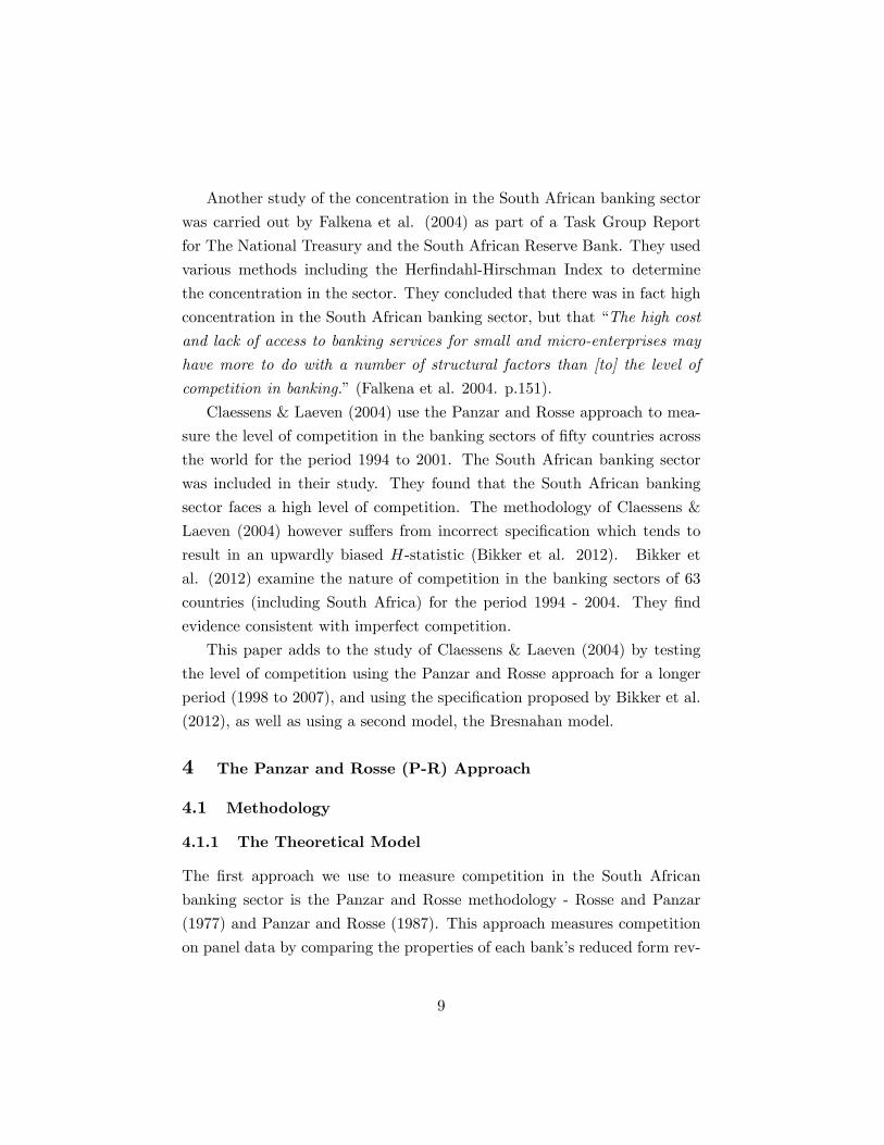
Another study of the concentration in the South African banking sector

was carried out by Falkena et al. (2004) as part of a Task Group Report

for The National Treasury and the South African Reserve Bank. They used

various methods including the Her�ndahl-Hirschman Index to determine

the concentration in the sector. They concluded that there was in fact high

concentration in the South African banking sector, but that �The high cost

and lack of access to banking services for small and micro-enterprises may

have more to do with a number of structural factors than [to] the level of

competition in banking.�(Falkena et al. 2004. p.151).

Claessens & Laeven (2004) use the Panzar and Rosse approach to mea-

sure the level of competition in the banking sectors of �fty countries across

the world for the period 1994 to 2001. The South African banking sector

was included in their study. They found that the South African banking

sector faces a high level of competition. The methodology of Claessens &

Laeven (2004) however su¤ers from incorrect speci�cation which tends to

result in an upwardly biased H-statistic (Bikker et al. 2012). Bikker et

al. (2012) examine the nature of competition in the banking sectors of 63

countries (including South Africa) for the period 1994 - 2004. They �nd

evidence consistent with imperfect competition.

This paper adds to the study of Claessens & Laeven (2004) by testing

the level of competition using the Panzar and Rosse approach for a longer

period (1998 to 2007), and using the speci�cation proposed by Bikker et al.

(2012), as well as using a second model, the Bresnahan model.

4 The Panzar and Rosse (P-R) Approach

4.1 Methodology

4.1.1 The Theoretical Model

The �rst approach we use to measure competition in the South African

banking sector is the Panzar and Rosse methodology - Rosse and Panzar

(1977) and Panzar and Rosse (1987). This approach measures competition

on panel data by comparing the properties of each bank�s reduced form rev-

9

enue equation across time. Two of the important assumptions underpinning

this model are (i) that banks operate in their long run equilibrium and (ii)

that all banks hold a homogeneous cost structure.12

The P-R model measures the level of competition by establishing how

each of the individual banks� revenues react to proportionate changes in

input prices. If the banks act as monopolies or at least in a monopolistic

manner, and face positive marginal costs, they will produce where demand

is elastic. An increase in input prices will increase marginal costs, causing

equilibrium output to decrease and equilibrium price to increase. Given that

their elasticity of demand is greater than unity, the increase in prices will

result in a reduction in the total revenue of the bank. This reduction in

revenue reveals that banks are acting in an anticompetitive manner.

In a perfectly competitive environment, an increase in input prices leads

to a rise in both marginal and average costs, with no change in the optimal

output for the individual banks.13 Theoretically, some banks should exit

the market, allowing the demand faced by the remaining banks to increase.

This should result in a proportionate increase in prices and revenues. The

percentage increase in revenues should be exactly equal to the percentage in-

crease in marginal costs in the case of a perfectly competitive market (Bikker

& Haaf, 2002). However, as shown by Bikker et al. (2012), if �rms face con-

stant average costs, it is possible that revenues will decrease following an

increase in input prices �negatively impacting the discriminating power of

the P-R methodology. Should the industry environment be that of monop-

olistic competition, the revenue will still increase by the same mechanism as

in perfect competition, but not by as much as the increase in marginal cost.

The more competitive the market, the more the revenues will increase as a

result of an increase in input prices.14

12However, the long run equilibrium hypothesis is not a prerequisite when testing formonopoly (Panzar and Rosse (1987: 446)).13This hinges on the assumptions of linear homogeneity of the cost function and long

run equilibrium.14This however must be quali�ed as the cost structure may disallow full pass-through of

input prices to revenues even for �rms in long-run competitive equilibrium, as shown byBikker et al. (2012). Thus the extent of pass-through is not necessarily that informativeregarding the nature of competition.

10

By maximising pro�ts at both the individual bank and industry level,

the equilibrium output and equilibrium number of banks can be found. At

the bank level, marginal revenues must equal marginal costs in order to

maximise each bank�s individual pro�ts, therefore

R0i(xi; n; zi)� C 0i(xi; wi; ti) = 0;

where R0i and C0i are the marginal revenue and marginal cost of bank i

respectively. The marginal revenue of bank i is a function of their output

(xi) and a vector of variables that shift their revenue function exogenously

(zi), as well as the number of banks (n). The marginal cost of bank i is a

function of their output, a vector of m factor input prices faced by the bank

(wi), and a vector of variables that shift their cost function exogenously (ti).

Furthermore, in order to determine the optimal number of banks,15 the

zero pro�t constraint must also hold at the industry level. Therefore

R�i (x�; n�; z)� C�i (x�; w; t) = 0;

where the superscript * denotes equilibrium values.

Panzar and Rosse have de�ned an H -statistic as the sum of the elasticity

of the banks� revenue with respect to a change in each of m factor input

prices. The H -statistic is therefore

H =

mXk=1

��R�i�wki

� wkiR�i

�;

where R�i is the equilibrium revenue for bank i and wki is the input price of

factor k for bank i.

The H -statistic derived by Panzar and Rosse is roughly speaking pos-

itively related to the level of competition in the banking sector. The in-

terpretation of the H-statistic is a bit complicated however, in the sense

that several situations may arise. For instance, H � 0 may indicate either15 If this condition does not hold at the industry level, banks will realise potential pro�ts

(losses) and enter (leave) the market until the equilibrium number of banks is obtained.This zero pro�t constraint holds at this equilibrium.

11

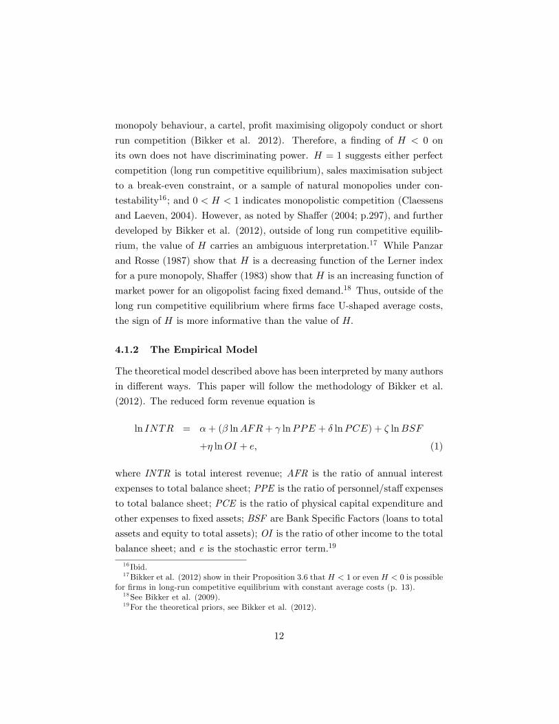
monopoly behaviour, a cartel, pro�t maximising oligopoly conduct or short

run competition (Bikker et al. 2012). Therefore, a �nding of H < 0 on

its own does not have discriminating power. H = 1 suggests either perfect

competition (long run competitive equilibrium), sales maximisation subject

to a break-even constraint, or a sample of natural monopolies under con-

testability16; and 0 < H < 1 indicates monopolistic competition (Claessens

and Laeven, 2004). However, as noted by Sha¤er (2004; p.297), and further

developed by Bikker et al. (2012), outside of long run competitive equilib-

rium, the value of H carries an ambiguous interpretation.17 While Panzar

and Rosse (1987) show that H is a decreasing function of the Lerner index

for a pure monopoly, Sha¤er (1983) show that H is an increasing function of

market power for an oligopolist facing �xed demand.18 Thus, outside of the

long run competitive equilibrium where �rms face U-shaped average costs,

the sign of H is more informative than the value of H:

4.1.2 The Empirical Model

The theoretical model described above has been interpreted by many authors

in di¤erent ways. This paper will follow the methodology of Bikker et al.

(2012). The reduced form revenue equation is

ln INTR = �+ (� lnAFR+ lnPPE + � lnPCE) + � lnBSF

+� lnOI + e; (1)

where INTR is total interest revenue; AFR is the ratio of annual interest

expenses to total balance sheet; PPE is the ratio of personnel/sta¤ expenses

to total balance sheet; PCE is the ratio of physical capital expenditure and

other expenses to �xed assets; BSF are Bank Speci�c Factors (loans to total

assets and equity to total assets); OI is the ratio of other income to the total

balance sheet; and e is the stochastic error term.19

16 Ibid.17Bikker et al. (2012) show in their Proposition 3.6 that H < 1 or even H < 0 is possible

for �rms in long-run competitive equilibrium with constant average costs (p. 13).18See Bikker et al. (2009).19For the theoretical priors, see Bikker et al. (2012).

12

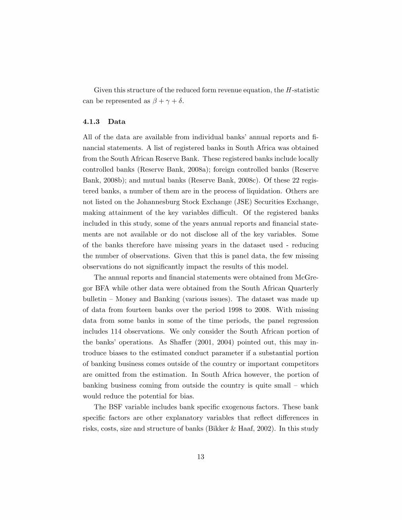
Given this structure of the reduced form revenue equation, theH -statistic

can be represented as � + + �.

4.1.3 Data

All of the data are available from individual banks�annual reports and �-

nancial statements. A list of registered banks in South Africa was obtained

from the South African Reserve Bank. These registered banks include locally

controlled banks (Reserve Bank, 2008a); foreign controlled banks (Reserve

Bank, 2008b); and mutual banks (Reserve Bank, 2008c). Of these 22 regis-

tered banks, a number of them are in the process of liquidation. Others are

not listed on the Johannesburg Stock Exchange (JSE) Securities Exchange,

making attainment of the key variables di¢ cult. Of the registered banks

included in this study, some of the years annual reports and �nancial state-

ments are not available or do not disclose all of the key variables. Some

of the banks therefore have missing years in the dataset used - reducing

the number of observations. Given that this is panel data, the few missing

observations do not signi�cantly impact the results of this model.

The annual reports and �nancial statements were obtained from McGre-

gor BFA while other data were obtained from the South African Quarterly

bulletin �Money and Banking (various issues). The dataset was made up

of data from fourteen banks over the period 1998 to 2008. With missing

data from some banks in some of the time periods, the panel regression

includes 114 observations. We only consider the South African portion of

the banks�operations. As Sha¤er (2001, 2004) pointed out, this may in-

troduce biases to the estimated conduct parameter if a substantial portion

of banking business comes outside of the country or important competitors

are omitted from the estimation. In South Africa however, the portion of

banking business coming from outside the country is quite small �which

would reduce the potential for bias.

The BSF variable includes bank speci�c exogenous factors. These bank

speci�c factors are other explanatory variables that re�ect di¤erences in

risks, costs, size and structure of banks (Bikker & Haaf, 2002). In this study

13

we use two bank speci�c ratios: Equity to Total Assets (BSF-EQ) and Loans

to Total Assets (BSF-LO).20 The inclusion of the non-performing loans ratio

reduces the sample size to half. It was decided that the bene�t of this gain

in a control variable does not outweigh the loss of power of the model. This

variable was therefore excluded from the regression.

4.2 Empirical Results

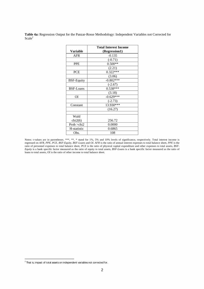
We estimate the unscaled revenue equation as proposed by Bikker et al.

(2012) using the feasible generalised least squares (FGLS) method. Total

interest income is regressed on bank input prices (price of deposits (AFR),

wage rate (PPE), and price of capital (PCE)), and control variables (credit

risk (BSF-LO), leverage (BSF-EQ), and other income (OI)). We �rst esti-

mate the unscaled revenue equation as given in (1) above. The results are

reported in Table 4a. The coe¢ cient on the average funding rate is negative

(-0.134) but insigni�cant, the wage rate is positive (0.50) and signi�cant at

the 5% level; the price of physical capital is also positive (0.32) and signi�-

cant at the 5% level. All the control variables are signi�cant and the signs

are consistent with the theory. In particular, BSF-LO is positive, suggesting

that a higher loans to total assets ratio raises interest income, BSF-EQ car-

ries a negative sign, indicating that lower leverage reduces interest income,

and OI has a negative impact on interest income as expected. The associ-

ated P-R statistic �which is given by the summation of the input elasticities

�is given by H = 0:69.

Table 4a about here.

A concern raised in Bikker et al. (2012) is that even though the estimated

equation is an unscaled equation, there are implicit scale e¤ects as some of

the right hand variables such as BSF-LO and BSF-EQ have total assets as

a denominator. To address this concern, we check for correlations between

20Bikker and Haaf (2001) used, in addition to the risk component, the di¤erences indeposit mix control and the divergent correspondent activities control. However, due tothe unavailability of data, these variables cannot be computed for South Africa.

14

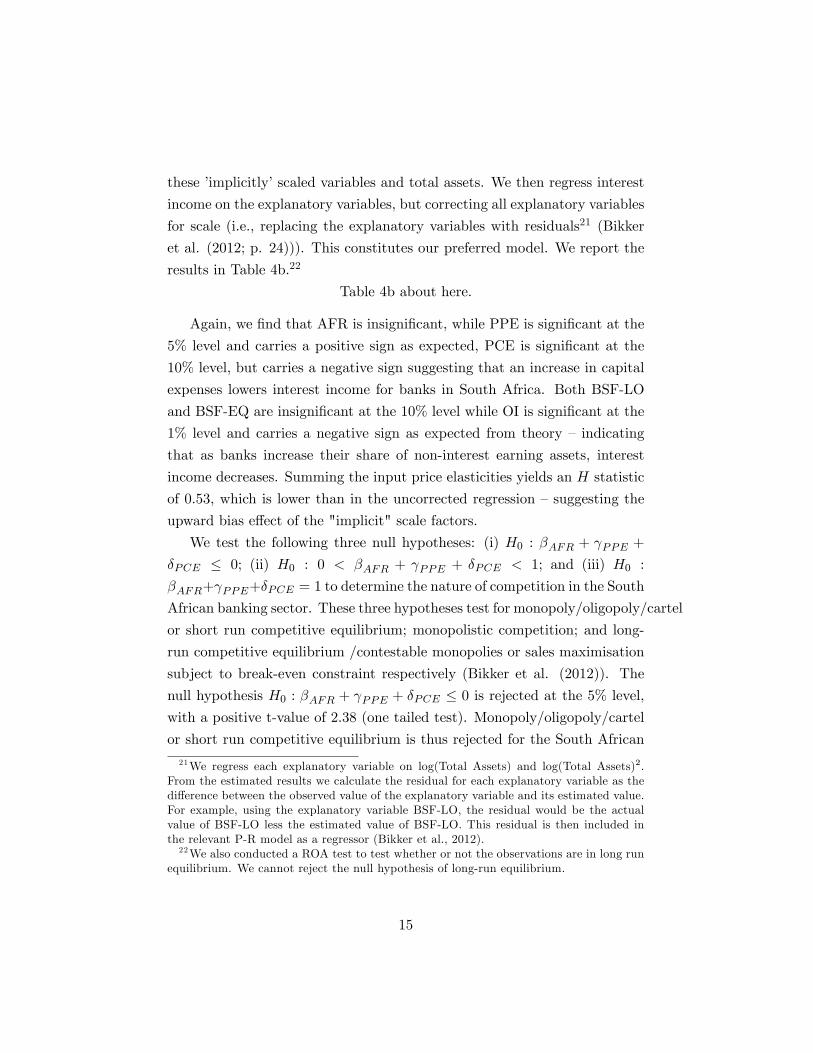
these �implicitly�scaled variables and total assets. We then regress interest

income on the explanatory variables, but correcting all explanatory variables

for scale (i.e., replacing the explanatory variables with residuals21 (Bikker

et al. (2012; p. 24))). This constitutes our preferred model. We report the

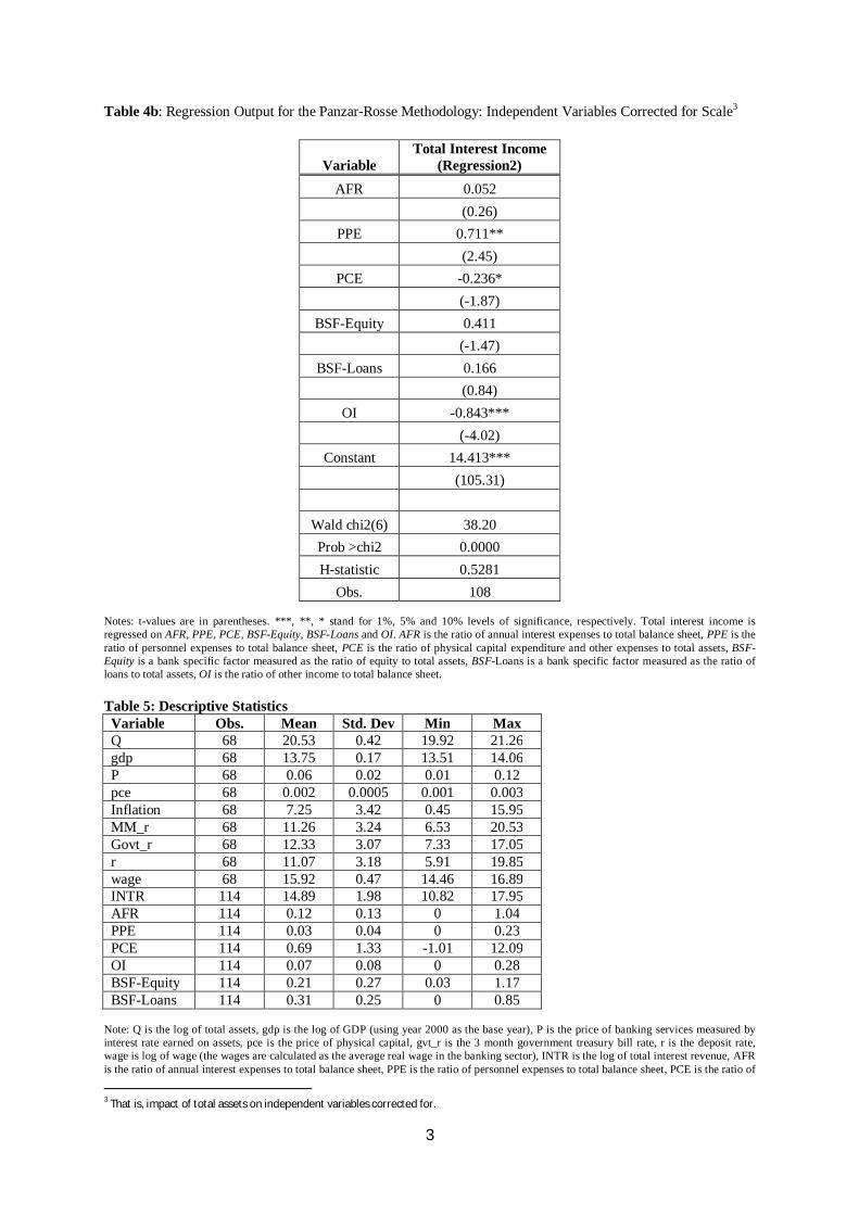
results in Table 4b.22

Table 4b about here.

Again, we �nd that AFR is insigni�cant, while PPE is signi�cant at the

5% level and carries a positive sign as expected, PCE is signi�cant at the

10% level, but carries a negative sign suggesting that an increase in capital

expenses lowers interest income for banks in South Africa. Both BSF-LO

and BSF-EQ are insigni�cant at the 10% level while OI is signi�cant at the

1% level and carries a negative sign as expected from theory � indicating

that as banks increase their share of non-interest earning assets, interest

income decreases. Summing the input price elasticities yields an H statistic

of 0:53, which is lower than in the uncorrected regression �suggesting the

upward bias e¤ect of the "implicit" scale factors.

We test the following three null hypotheses: (i) H0 : �AFR + PPE +

�PCE � 0; (ii) H0 : 0 < �AFR + PPE + �PCE < 1; and (iii) H0 :

�AFR+ PPE+�PCE = 1 to determine the nature of competition in the South

African banking sector. These three hypotheses test for monopoly/oligopoly/cartel

or short run competitive equilibrium; monopolistic competition; and long-

run competitive equilibrium /contestable monopolies or sales maximisation

subject to break-even constraint respectively (Bikker et al. (2012)). The

null hypothesis H0 : �AFR + PPE + �PCE � 0 is rejected at the 5% level,

with a positive t-value of 2.38 (one tailed test). Monopoly/oligopoly/cartel

or short run competitive equilibrium is thus rejected for the South African

21We regress each explanatory variable on log(Total Assets) and log(Total Assets)2.From the estimated results we calculate the residual for each explanatory variable as thedi¤erence between the observed value of the explanatory variable and its estimated value.For example, using the explanatory variable BSF-LO, the residual would be the actualvalue of BSF-LO less the estimated value of BSF-LO. This residual is then included inthe relevant P-R model as a regressor (Bikker et al., 2012).22We also conducted a ROA test to test whether or not the observations are in long run

equilibrium. We cannot reject the null hypothesis of long-run equilibrium.

15

banking sector. The null hypothesis H0 : �AFR + PPE + �PCE = 1 is

also rejected at the 5% level (p = 0:019), implying that the H -statistic is

statistically di¤erent from one (more precisely, smaller than unit, as it is a

one-tailed test). However, without information on the cost structure of the

banking sector, there is not su¢ cient information for us to conclude that

long run competitive equilibrium is rejected. We also tested for the null

hypothesis of monopolistic competition, H0 : 0 < �AFR+ PPE+�PCE < 1;

and we cannot reject this null hypothesis. We thus conclude that the South

African banks face monopolistic competition.

The result of this application of the Panzar and Rosse approach reveals

that, with regard to interest income, the South African banking sector is

monopolistic competition in nature. Thus banks appear to posses some

degree of market power, but do not operate as �absolute�monopolies. The

results of our study are relatively similar to the �ndings of Bikker et al.

(2012) who �nd an H�statistic of 0:46 for South Africa.23

That personnel costs signi�cantly explain interest income is interesting.

There are debates currently in South Africa around �nancialisation of the

economy. Concerns are that the �nancial sector is growing too fast, and

at the expense of other sectors, as it has been able to attract skills from

other sectors through its ability to pay higher wages. The high degree of

concentration and the high switching costs and complex bank products help

explain the monopolistic outcome (Jali et al. 2008). Indeed, despite the high

concentration, non-price competition appears to be signi�cant, for example,

advertising.

23A caveat is in order. As discussed in section 4.1.1, any value of H di¤erent from 1 isdi¢ cult to interpret as di¤erent levels of market power are consistent with such values. Seefor instance, Sha¤er (2004); Bikker et al. (2012). In particular, the relationship betweenH and the degree of competition is non-monotonic.

16

5 The Bresnahan Model

5.1 Methodology

5.1.1 The Theoretical Model

The second model that is used to measure competition in the South African

banking sector is the Bresnahan Model (Bresnahan (1982)). This is a non-

structural test for the degree of competitiveness, such that this model can

be used even when there is no cost or pro�t data available. This can be

done by using industry aggregate data to measure this competition.

The idea behind the Bresnahan approach is to see how price and quan-

tity react to changes in exogenous variables - revealing the degree of market

power of the average bank, and hence the level of competition in the banking

industry. In particular, rotations of the demand curve around the equilib-

rium point (i.e., changes in demand slope) - induced by changes in exogenous

variables - will discriminate between the di¤erent forms of market conduct

(Bresnahan, 1982: 92-93).

More formally, let the pro�t function for the average bank take the form

(Bikker, 2003):

�i = pxi � ci(xi; EXS); 24

where �i is pro�t; xi is the quantity of output of the bank; p is the output

price; and ci are the variable costs faced by bank i. The variable costs are a

function of the output of the bank, as well as the exogenous variables that

a¤ect marginal costs, but not the industry demand function (EXS).

The inverse of the demand function faced by the banks is

p = f(X;EXD) = f(x1 + x2 + : : :+ xn; EXD);

such that prices are a function of exogenous variables that a¤ect the industry

demand but not the marginal cost (EXD) and each of the n banks�outputs.

24We abstract from �xed costs as they do not in�uence the bank�s optimising behaviour.

17

The �rst order conditions for pro�t maximization of bank i is

d�idxi

= p+ f 0(X;EXD)dX

dxixi � c0(xi; EXS) = 0:

Summing over all banks gives

p+ f 0(X;EXD)dX

dxi

1

nX � c0(xi; EXS) = 0;

such that

p = ��f 0(X;EXD)X + c0(xi; EXS); (2)

where � is the measure of the level of competition in the banking sector and

is equal to

� =dX

dxi

1

n=

�1 +

dPj 6=i xj

dxi

�1

n:

In this case, � is a �function of the conjectural variation25 of the average �rm

in the market�(Bikker & Haaf, 2001). In a perfectly competitive industry,

an increase in the output of bank i should result in a decrease of all other

banks�outputs totalling the same magnitude as the initial increase in bank

i�s output. Thus � =�1 +

dPj 6=i xjdxi

�1n = (1 � 1)

1n = 0, irrespective of the

number of banks, n. If there is perfect collusion in the industry, an increase

in bank i�s output will result in an equal increase in the output of all the

other banks in the industry. This means thatdPj 6=i xjdxi

= X�xixi

and as a

result � = Xxin

= 1. For a single monopolist, there are no other banks in

the industry and thusdPj 6=i xjdxi

= 0. Therefore � = 1n where n = 1, from

which � = 1. Under the usual assumptions, these are the two extreme values

of � corresponding to opposite levels of competition in the industry. The

conduct parameter � is restricted between 0 and 1, and is proportional to

the level of competition in the industry.

25Conjectural variation is the change in output of the other banks, anticipated by banki as a response to an initial change in its own output.

18

5.1.2 The Empirical Model

As is standard in the literature, we consider deposits as an input rather than

an output of the bank. We consider the bank�s output to be loans, and the

demand for loans is given by,

Q = �0 + �1P + �2EXD + �3EXDP + �; (3)

where Q is the real value of total assets (a proxy for loans) in the industry

(used to measure banking services or output); P is the price of the banking

services; EXD are the exogenous variables that a¤ect industry demand for

banking services, but not the marginal costs - including disposable income,

number of bank branches and interest rates for alternative investments (the

money market rate and the government bond rate); and � is the error term.

The interaction terms EXDP are included to ensure the identi�cation of the

conduct parameter, �:Without the interaction terms, one cannot distinguish

competition from monopoly (Bresnahan, 1982: 152-153).

On the supply side, Bikker and Haaf (2002) as well as Sha¤er (1993)

postulate the following marginal cost function:26

MC = �0 + �1InQi +�j�j lnEXSj ; (4)

where MC is the marginal cost for each bank; EXS are the exogenous

variables that in�uence the supply of loans, including the cost of input fac-

tors for the production of loans - wages, deposit rate and price of physical

capital. The cost function as speci�ed, is a legitimate marginal cost function

as it satis�es all the requisite properties.

Rearranging the demand function yields,

P =1

�1 + �3EXD[Q� �0 � �2EXD � �] : (5)

The total revenue for each bank can be obtained by multiplying the above

26There is no requirement that the "true" marginal cost be linear. We can view (4) asa linear approximation of the marginal cost function.

19

rearranged demand equation by bank i�s output, Q,

TRi =1

�1 + �3EXD[Q� �0 � �2EXD � �]Q: (6)

Di¤erentiating this total revenue with respect to bank i�s output will give

the bank�s marginal revenue,

MRi =dTRidQi

=1

�1 + �3EXD[Q� �0 � �2EXD � �]

+1

�1 + �3EXD

dQ

dQiQi

= P +�n

�1 + �3EXDQi: (7)

Equating the marginal revenue and marginal cost of each bank to obtain the

market equilibrium yields,

P +�n

�1 + �3EXDQ = �0 + �1 lnQ+�j�j lnEXSj + vi: (8)

Rearranging and averaging to obtain the supply of loan facilities by the

banks yields:

P = �� Q

�1 + �3EXD+ �0 + �1 lnQ+�j�j lnEXSj + v: (9)

Equations (3) and (9) constitute a system of two equations which we need

to estimate to determine the � statistic.27 We thus have a simultaneous

equation system and because of the possible endogeneity problem, equations

(3) and (9) are estimated simultaneously to identify �:

5.1.3 The � Statistic

This coe¢ cient � is the value that determines the level of competition in

the banking sector. Speci�cally, � indexes the degree of market power of the

27 Identi�cation of � requires that both �1 6= 0 and �3 6= 0 holds.

20

average bank (Sha¤er, 2001). If � = 0; the outcome is competitive while � =

1 if the outcome is perfectly collusive. For � 2 (0; 1) ; the banking marketis imperfectly competitive, and allows for all forms of oligopoly behaviour

(see Sha¤er (2001) for further explanations).

The estimated equations are:

Q = a0 + a1P + a2gdp+ a3Pgdp+ a4govt_r + a5Pgovt_r + �; (10)

P =��Q

a1 + a3gdp+ a5govt_r+b0+b1 lnQ+b2 lnwage+b4 ln r+b5 ln pce+v;

(11)

where Q is the quantity of banking services measured as the dollar value

of total assets and P is the pricing of banking services measured by the

interest rate earned on the assets; gdp is the real gross domestic product,

govt_r is the 3 month government treasury bill rate, Pgovt_r and Pgdp

are interaction terms; wage is the average real wage in banking sector and

r is the deposit rate and pce is the price of physical capital. The variable,

Q� 1a1+a3gdp+a5govt_r

is the conduct variable and its coe¢ cient, ��, is theparameter of interest. The parameters � and v are the respective error terms.

The speci�cation of the � parameter implicitly assumes that banks are

input-price takers �which is plausible for labour and physical capital since

in South Africa banks compete with other �rms for labour and capital. For

deposits however, the case may be di¤erent. It is possible that the deposit

rate may be exogenous, if there is sti¤ competition for deposits (Sha¤er;

1993, 2004). In that case the above assumptions still hold and banks would

still be input price-takers even when it comes to deposits. However if banks

have market power in deposits then the � as speci�ed in the model may over-

state the degree of market power and thus be biased against the competitive

case (Sha¤er, 1993).

5.1.4 Data

The data required for the Bresnahan model are all macroeconomic (industry

level) time series variables. Macroeconomic data is generally easier to obtain

21

than microeconomic data. This is one of the bene�ts of using the Bresnahan

model versus models that use bank speci�c data such as the Panzar and

Rosse approach. In the case of a developing country such as South Africa

however, this data is not always readily available. For example, there is

not su¢ cient data to enable us to test directly competition for the loans

market. Following Sha¤er (1993) we use the value of total assets as a proxy

for output since we do not have su¢ cient information on loans.

Unfortunately, historical unemployment data is not readily available for

South Africa. The longest range was available from the International Mon-

etary Fund�s International Financial Statistics (IFS) database which con-

tained quarterly data from Q1 of 1992 until Q4 of 2008. This dataset has a

two year gap from Q1 of 1998 until Q4 of 1999. This therefore would restrict

the study to 57 periods. Since our sample is already small, we decided to

drop the unemployment variable from the sample in order to raise the num-

ber of observations. Most of the remaining variables were also obtained from

the IFS database. The banking sector wage variable was obtained from the

South African Reserve Bank online database. Disposable income data was

only available annually from the South African Reserve Bank database. Im-

puting quarterly values would result in inaccurate data, therefore a proxy

for the disposable income was used. The best proxy would be the Gross

Domestic Product (GDP) at constant 2000 prices. This is because the dis-

posable income is calculated from the GDP by subtracting aggregate taxes

from this value.28 There was insu¢ cient time series data on the number of

bank branches, therefore this variable was excluded from this study. Table

5 below provides some descriptive statistics.

Table 5 about here.

5.2 Empirical Results

The quantity of banking services is determined by the price of banking

services and exogenous variables such as GDP and government treasury bill

28Bikker & Haaf (2002) also used GDP as a proxy for disposable income.

22

rate. The price coe¢ cient should be consistent with a downward-sloping

demand curve. The government debt rate, being a price of a substitute,

should have a negative coe¢ cient. GDP proxies for income and it is expected

to be positive.

The supply equation (9) determines the price of banking services as a

function of the volume of banking services (Q), the price of inputs (wage

rate, price of physical capital and deposit rate), and the output times the

�rst derivative of the demand function. The estimated coe¢ cients of wages

of bank employees, interest rate on deposits (r), and price of physical capital

should be positive �showing that higher costs will be passed on to consumers

in the form of higher price of loans. The coe¢ cient on �output times the

inverse of the �rst derivative of the demand function� is the parameter of

interest in this exercise. It gives a measure of the degree of market power of

the average bank.

We estimate equations (10) and (11) and the outputs are reported in

the Tables 6a and 6b below.29 Given that P (an endogenous variable in the

supply equation) appears as a regressor in the demand equation (10) and

likewise Q (endogenous) appears as a regressor in the supply equation, we

have a (possible) simultaneity problem. In this case, estimating by OLS may

result in inconsistent and/or ine¢ cient estimates for at least two reasons:

First, one or more of the endogenous variables may be correlated with the

error term and second, the error terms may themselves be correlated. We

ran some endogeneity tests - speci�cally the Hausman test and the Durbin-

Wu-Hausman test. The test results suggest no endogeneity. However, the

identi�cation conditions for the conduct parameter (a3 6= 0 and/or a5 6= 0)are not met at the 5% signi�cance level. The joint test of a3 = a5 = 0

cannot be rejected at the 10% level. However, individual tests show that

a3 = 0 is rejected at the 10% level while a5 = 0 cannot be rejected at

the 10% level. Given these weak identi�cation results and our intuition29The Augmented Dickey-Fuller test identi�ed that each variable is integrated at the

�rst di¤erence, with unit roots at the levels. The Pesaran-Shin-Smith ARDL showed aunique long-run relationship, allowing the conduct variable to be interpreted as if no timeseries characteristics exist.

23

on the equilibrium relationship between demand and supply, we proceeded

to estimate the demand and supply equations simultaneously using a SAS

programme.

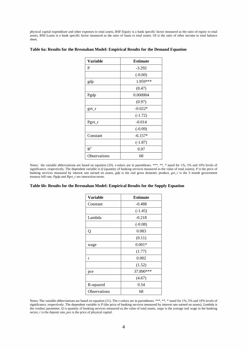
Tables 6a and 6b about here.

For the demand equation, GDP is positive and signi�cant at the 1% level

while the government rate (Govt_r) is only signi�cant at the 10% level, but

carries the correct (negative) sign. Price carries the correct (negative) sign

but is insigni�cant. The coe¢ cients on the interaction terms PGovt_r and

PGDP , are insigni�cant at the 10% level.

In the supply equation, the input price coe¢ cients carry the expected

(positive) signs �suggesting that higher prices of inputs raise the price of

loans. However, only two coe¢ cients are signi�cant: wages are signi�cant

at the 10% level only while price of capital is signi�cant at the 1% level.

The parameter of interest in this exercise is the coe¢ cient of the conduct

variable, ��. The estimation yields � equal to 0.2, with a t-statistic of -0.08. The � statistic is thus insigni�cant �implying that the coe¢ cient is

statistically equal to zero.30 This insigni�cant coe¢ cient means that � � 0;and that according to the Bresnahan model, perfect competition cannot be

rejected in the South African banking sector. This however does not imply

competitive conduct by the South African banks as failure to reject perfect

competition does not mean acceptance of competition or evidence of no

market power.31

The results of the Bresnahan model in general, and in the present paper

in particular, should be interpreted with caution for a number of reasons.

Among these are that the data are generally imprecise and fraught with

measurement errors and our sample is too short. In addition, the Bresna-

han methodology appears to have weak discriminating power in practice.

Even more pertinent to the present study, the model is not identi�ed at

the (standard) 5% signi�cance level, but only at the 10% signi�cance level -

30This insigni�cant coe¢ cient does not seem to be a problem as the output for theBresnahan model in Sha¤er (1989) on the U.S. banking sector, and the � coe¢ cients ofall of the countries in Bikker & Haaf (2002) are also insigni�cant.31The authors thank an anonymous referee for highlighting this observation to us.

24

suggesting less con�dence in the determination of signi�cance (i.e., greater

likelihood of committing a Type I error).

6 Comparison with other Developing Countries

Many studies have been conducted using di¤erent methods to �nd the level

of competition in the banking sectors of numerous countries across the world.

The two main approaches used are the two methods applied in this paper,

the Panzar and Rosse approach and the Bresnahan model.32

Perera et al. (2006) have used the Panzar and Rosse approach on some

developing Asian countries including Bangladesh, India, Pakistan and Sri

Lanka. Claessens & Laeven (2004) have conducted the Panzar and Rosse

approach on �fty countries around the world, of which thirty one are devel-

oping countries. Recently, Bikker et al. (2012) use a much larger sample to

estimate the H -statistics for di¤erent countries �developing and developed.

They �nd an H -statistic of 0.46 for South Africa.

The countries that are most comparable to South Africa in terms of their

level of development include Argentina, Brazil, Chile and Turkey. The H -

statistics for these range between 0.21 for Chile to 0.61 for Turkey. These

results suggest that these �ve countries all have low to moderate level of

competition in their respective banking sectors.

These results are however markedly di¤erent to those of Claessens &

Laeven (2004) and earlier studies who estimate a scaled revenue equation.

For instance, Claessens & Laeven (2004) �nd an H -statistic of 0.85 for South

Africa, and fairly high H -values for Chile, Argentina and Brazil (0.66, 0.73

and 0.83 respectively), but a moderate H -value for Turkey (0.46).

7 Conclusion

32Generally, the results of the Bresnahan approach are less robust than those of thePanzar-Rosse model, largely due to measurement errors in variables and weak discrimi-nating power.

25

Given the importance of the banking sector on the economic perfor-

mance of any modern economy, it is imperative that the banking sector is

competitive. This will help improve the e¢ ciency required to create a fully

functional credit system as well as strengthen the e¤ectiveness of monetary

policy.

This paper has used two non-structural models to test for the level of

competition in the South African banking sector. The Panzar and Rosse

model suggests imperfect competition in the South African banking sector

while the Bresnahan model fails to reject perfect competition. Although

the results of the Bresnahan model for South Africa should be interpreted

with caution (model is only identi�ed at the 10% signi�cance level and not

at the (standard) 5% signi�cance level), the fact that the results are not

inconsistent with the more reliable Panzar-Rosse model is encouraging. The

results of the models combined with support from other recent applications

of these models, as well as the similar results for comparable developing

countries, suggests behaviour consistent with monopolistic competition in

the South African banking sector.

The �nding of monopolistic competition in the South African banking

sector is likely to be "welcomed" consumers and South African authorities

(South African banks are not acting as a cartel), especially given the dom-

inance of the four largest banks in South Africa. While this (absence of

cartel) may be the case over the study period, the scope for collusion is a

risk that should continually be managed, given the high concentration. Pol-

icy makers and sector regulators should thus remain vigilant. In addition,

the �nding of monopolistic competition suggests a need for policies to bring

about more contestability in the banking sector. The general implication of

the �ndings of this study is that regulators and policy makers should not

obsess with reducing banking sector concentration per se - as competition

and concentration are not mutually exclusive. Instead, e¤orts need to be

focused on measures that facilitate competition; for example policies that

lower switching costs for consumers or lock-ins. Also, our �ndings provide

evidence to the theoretical �nding of no obvious casual relationship between

structure and conduct.

26

References

[1] ABSA Annual Report (2011). ABSA Integrated Annual Re-

port, 31 December 2011. Retrieved on 10 January 2013

from http://www.absa.co.za/Absacoza/About-Absa/Investor-

Relations/Annual-Reports.

[2] Albaek, S., Mollgaard, P. and Overgaard, Per B., (2003). Government-

Assisted Oligopoly Coordination? A Concrete Case. Journal of Indus-

trial Economics 45(4), 429-443.

[3] Bain, J. (1951). Relation of Pro�t Rate to Industry Concentration.

Quarterly Journal of Economics, No. 65 , 293-324.

[4] Baumol, W. (1982). Contestable Markets: An Uprising in the Theory

of Industry Structure. American Economic Review, Vol. 72 , 1-15.

[5] Berger, A.N. (1995). The Pro�t-Structure Relationship in Banking -

Tests of Market Power and E¢ cient-Structure Hypothesis. Journal of

Money, Credit, and Banking 27, 404-431.

[6] Berger, A.N., & Hannan, T. (1989). The Price-Concentration Relation-

ship in Banking. The Review of Economics and Statistics, No. 71 ,

291-299.

[7] Bikker, J.A., (2003). Testing for imperfect competition on EU deposit

and loan markets with Bresnahan�s market power model. Kredit und

Kapital 36, 167-212.

[8] Bikker, J., & Haaf, K. (2001). Measure of Competition and Concen-

tration: A Review of the Literature. De Nederlandsche Bank Research

Supervision Studies, No. 27.

[9] Bikker, J., & Haaf, K. (2002). Competition, Concentration and their

Relationship: An Empirical Analysis of the Banking Industry. Journal

of Banking & Finance, Elsevier, Vol. 26(11) , 2191-2214.

27

[10] Bikker, J.A., S. Sha¤er and L. Spierdijk (2009). �The Panzar�Rosse

Revenue Test: To Scale or Not to Scale�, 22nd Australasian Finance

and Banking Conference, 21 August.

[11] Bikker, J.A., Sha¤er, S., and Spierdijk, L., (2012). Assessing Compe-

tition with the Panzar-Rosse Model: The Role of Scale, Costs, and

Equilibrium. Forthcoming, Review of Economics and Statistics.

[12] Bresnahan, T.F., (1982). The Oligopoly Solution Concept is Identi�ed.

Economics Letters 10 , 87-92.

[13] Bresnahan, T.F., 1989, Empirical studies of industries with market

power, in: Schmalensee, R., Willig, R.D. (Eds): Handbook of Indus-

trial Organisation, Volume II, 1012-1055.

[14] Claessens, S., & Laeven, L. (2004). What Drives Bank Competition?

Some International Evidence. Journal of Money, Credit and Banking,

Vol. 36, No. 3, 563-583.

[15] Claessens, S., & Laeven, L. (2005). Financial Dependence, Banking

Sector Competition, and Economic Growth. Journal of the European

Economic Association, Vol. 3, No. 1, 179-207.

[16] Demsetz, H. (1973). Industry Structure, Market Rivalry and Public

Policy. Journal of Law and Economics, No. 3 , 1-9.

[17] Falkena, H. et al.. (2004). Competition in South African Banking. Task

Group Report - The National Treasury and The South African Reserve

Bank.

[18] FNB Annual Report (2011). Firstrand Integrated An-

nual Report. Retrieved on 10 January 2013 from

http://www.�rstrand.co.za/InvestorCentre/Pages/annual-

reports.aspx.

[19] Grobbelaar, N., (2004). Can South Africa business drive regional in-

tegration on the continent? South African Journal of International

A¤airs, Vol. 1 (2), 91-106.

28

[20] Iwata, G. (1974). Measurement of Conjectural Variations in Oligopoly.

Econometrica, No. 42 , 947-966.

[21] Jali, T., Nyasulu, H., Bodibe, O., & Petersen, R. (2008). Banking En-

quiry. Competition Commission.

[22] Kot, A. (2004). Is interest rate pass-through related to banking sector

competitiveness? Working paper, National Bank of Poland.

[23] Lau, L. (1982). On Identifying the Degree of Competitiveness from

Industry Prices and Output Data. Economics Letters 10 , 93-99.

[24] Mullineux, A., & Sinclair, P. (2000). Oligopolistic Banks: Theory and

Policy Implications. Unpublished.

[25] Nedbank Annual Report (2011). Nedbank Limited Annual Report for

the year ended 31 December 2011. Retrieved on 10 January 2011 from

bhttp://www.nedbankgroup.co.za/pdfs/groupCompanies/nedbank_ar2011.pdf.

[26] Okeahalam, C. (1998). An Analysis of the Price-Concentration Rela-

tionship in the Botswana Commercial Banking Industry. Journal of

African Finance and Economic Development, No. 3 , 65-84.

[27] Okeahalam, C. (2001). Structure and Conduct in the Commercial Bank-

ing Sector of South Africa. Presented at TIPS 2001 Annual Forum.

[28] Panzar, J.C., & Rosse, J.N., (1987). Testing for �Monopoly�Equilib-

rium. The Journal of Industrial Economics. Vol. 35, No. 4 , 443-456.

[29] Perera, S., Skully, M., & Wickramanayake, J. (2006). Competition and

Structure of South Asian Banking: A Revenue Behavior Approach.

Applied Financial Economics 16 , 789-901.

[30] Ramjee, A., and Gwatidzo, T., (2012). Dynamics of capital structure

determinants in South Africa. Meditari Accountancy Research, Vol.

20(1), 52-67.

29

[31] Reserve Bank. (2008a). Registered Banks - Locally Con-

trolled. Retrieved January 2008, from Reserve Bank Website:

http://www2.resbank.co.za/33

[32] Reserve Bank. (2008b). Registered Banks - Foreign Con-

trolled. Retrieved January 2008, from Reserve Bank Website:

http://www2.resbank.co.za/34

[33] Reserve Bank. (2008c). Registered Mutual Banks. Retrieved January

2008, from Reserve Bank Website: http://www2.resbank.co.za/35

[34] Rosse, J.N., and Panzar, J.C., (1977). Chamberlin vs Robinson: An

empirical study for monopoly rents. Bell Laboratories Economic Dis-

cussion Paper, No. 90.

[35] Schmalensee, R., (1989). Interindustry studies of structure and per-

formance. In Schmalensee, R. and Willig, R. D. (Eds.): Handbook of

Industrial Organisation, Vol. II. North-Holland, Amsterdam.

[36] Sha¤er, S. (1983). The Panzar-Rosse statistic and the Lerner Index in

the short run, Economics Letters, 11, Issues 1-2, 175-178.

[37] Sha¤er, S. (1989). Competition in the U.S. Banking Industry. Eco-

nomics Letters 29 , 321-323.

[38] Sha¤er, S. (1993). A Test of Competition in Canadian Banking. Journal

of Money, Credit and Banking, Vol. 25(1) , 49-61.

[39] Sha¤er, S. (2001). Banking conduct before the European single bank-

ing licence: A cross-country comparison. North American Journal of

Economics and Finance, Vol. 12, 79-104.

33http://www2.resbank.co.za/BankSup/BankSup.nsf/$$ViewTemplate+for+Banks+-+Locally+Controlled?OpenForm34http://www2.resbank.co.za/BankSup/BankSup.nsf/$$ViewTemplate+for+Banks+-

+Foreign+Controlled?OpenForm35http://www2.resbank.co.za/BankSup/BankSup.nsf/$$ViewTemplate+for+Mutual+-

Banks?OpenForm

30

[40] Sha¤er, S. (2004). Patterns of competition in banking. Journal of Eco-

nomics and Business, Vol. 56, 287-213.

[41] Standard Bank Annual Report (2011). The Standard Bank of

South Africa Annual Report. Retrieved on 10 January 2011

fromhttp://reporting.standardbank.com/downloads/archive/2011/Standard_Bank_Plc_Consolidated_Annual_Report_2011.pdf.

[42] Tirole, J. (1988). The Theory of Industrial Organization. Cambridge,

MA: The MIT Press.

[43] Van Leuvensteijn, M., Kok-Sørensen, C., Bikker, J., & Van Rixtel, A.

(2008). Impact of Bank Competition on the Interest Rate Pass-Through

in the Euro Area. Working Paper Series, No. 885 - European Central

Bank.

[44] World Bank (2011). Global Statistics: Key indicators for country

groups and selected economies.

31

1

TABLES TABLE 1: The Reach of South African banks in Africa Name of South African Bank Other African Countries where the bank has operations

Standard Bank

Angola, Ghana, Malawi, Namibia, Swaziland, Lesotho, Mozambique, South Africa, Uganda, Zimbabwe, Tanzania, Nigeria, Mauritius, Kenya, Bots, Zambia, DRC

FNB Namibia, Botswana, Swaziland, Lesotho, Mozambique and Zambia.

Nedbank1

Angola, Benin, Burkina Faso, Burundi, Cape Verde, Cameroon, Central African Republic, Chad, Congo Brazzaville, Democratic Republic of Congo, Côte d'Ivoire, Equatorial Guinea, Gabon, Ghana, The Gambia, Guinea, Guinea Bissau, Kenya, Liberia, Malawi, Mali, Niger, Nigeria, Rwanda, Sao Tome & Principe, Senegal, Sierra Leone, Tanzania, Togo, Uganda, Zambia, Zimbabwe.

ABSA Ghana, Zambia, Botswana, Zimbabwe, Kenya, Uganda, Egypt, Mauritius, Seychelles.

Source: Standard Bank Annual Report (2011), FNB Annual Report (2011), ABSA Annual Report (2011), Nedbank Bank Annual Report (2011). TABLE 2 - Key Banking Values as a Percentage of GDP

2003 2004 2005 2006 2007

Total Deposits 72% 74% 80% 88% 93% Loans to Public Sector 6% 5% 5% 4% 3% Loans to Private Sector 58% 61% 67% 76% 81%

Source: The South African Reserve Bank Quarterly Bulletin - Money and Banking Online Database TABLE 3 - Market Share by Deposits and Total Assets (2007)

Name of Bank Total Deposits

(R Billion) % of Industry

Deposits Total Assets (R Billion)

% of Industry Assets

Standard Bank 705.84 36% 1175.41 36% Firstrand 416.51 21% 717.26 22% Nedbank 384.54 19% 483.61 14% ABSA 368.55 19% 640.61 19% Other Banks 96.24 5% 290.23 9% Total 1971.68 100% 3307.12 100%

Source: The South African Reserve Bank Quarterly Bulletin - Money and Banking Online Database 1 Through its Ecobank Nedbank Alliance, Nedbank has access to the client base in these countries.

2

Table 4a: Regression Output for the Panzar-Rosse Methodology: Independent Variables not Corrected for Scale2

Variable Total Interest Income

(Regression1) AFR -0.135

(-0.71)

PPE 0.500**

(2.21)

PCE 0.322***

(3.06)

BSF-Equity -0.802***

(-2.67)

BSF-Loans 0.538***

(3.18)

OI -0.629***

(-2.73)

Constant 13.930***

(16.27)

Wald chi2(6) 256.72

Prob >chi2 0.0000 H-statistic 0.6865

Obs. 108 Notes: t-values are in parentheses. ***, **, * stand for 1%, 5% and 10% levels of significance, respectively. Total interest income is regressed on AFR, PPE, PCE, BSF-Equity, BSF-Loans and OI. AFR is the ratio of annual interest expenses to total balance sheet, PPE is the ratio of personnel expenses to total balance sheet, PCE is the ratio of physical capital expenditure and other expenses to total assets, BSF-Equity is a bank specific factor measured as the ratio of equity to total assets, BSF-Loans is a bank specific factor measured as the ratio of loans to total assets, OI is the ratio of other income to total balance sheet. 2 That is, impact of total assets on independent variables not corrected for.

3

Table 4b: Regression Output for the Panzar-Rosse Methodology: Independent Variables Corrected for Scale3

Variable Total Interest Income

(Regression2) AFR 0.052

(0.26)

PPE 0.711**

(2.45)

PCE -0.236*

(-1.87)

BSF-Equity 0.411

(-1.47)

BSF-Loans 0.166

(0.84)

OI -0.843***

(-4.02)

Constant 14.413***

(105.31)

Wald chi2(6) 38.20 Prob >chi2 0.0000 H-statistic 0.5281

Obs. 108 Notes: t-values are in parentheses. ***, **, * stand for 1%, 5% and 10% levels of significance, respectively. Total interest income is regressed on AFR, PPE, PCE, BSF-Equity, BSF-Loans and OI. AFR is the ratio of annual interest expenses to total balance sheet, PPE is the ratio of personnel expenses to total balance sheet, PCE is the ratio of physical capital expenditure and other expenses to total assets, BSF-Equity is a bank specific factor measured as the ratio of equity to total assets, BSF-Loans is a bank specific factor measured as the ratio of loans to total assets, OI is the ratio of other income to total balance sheet. Table 5: Descriptive Statistics Variable Obs. Mean Std. Dev Min Max Q 68 20.53 0.42 19.92 21.26 gdp 68 13.75 0.17 13.51 14.06 P 68 0.06 0.02 0.01 0.12 pce 68 0.002 0.0005 0.001 0.003 Inflation 68 7.25 3.42 0.45 15.95 MM_r 68 11.26 3.24 6.53 20.53 Govt_r 68 12.33 3.07 7.33 17.05 r 68 11.07 3.18 5.91 19.85 wage 68 15.92 0.47 14.46 16.89 INTR 114 14.89 1.98 10.82 17.95 AFR 114 0.12 0.13 0 1.04 PPE 114 0.03 0.04 0 0.23 PCE 114 0.69 1.33 -1.01 12.09 OI 114 0.07 0.08 0 0.28 BSF-Equity 114 0.21 0.27 0.03 1.17 BSF-Loans 114 0.31 0.25 0 0.85

Note: Q is the log of total assets, gdp is the log of GDP (using year 2000 as the base year), P is the price of banking services measured by interest rate earned on assets, pce is the price of physical capital, gvt_r is the 3 month government treasury bill rate, r is the deposit rate, wage is log of wage (the wages are calculated as the average real wage in the banking sector), INTR is the log of total interest revenue, AFR is the ratio of annual interest expenses to total balance sheet, PPE is the ratio of personnel expenses to total balance sheet, PCE is the ratio of

3 That is, impact of total assets on independent variables corrected for.

4

physical capital expenditure and other expenses to total assets, BSF-Equity is a bank specific factor measured as the ratio of equity to total assets, BSF-Loans is a bank specific factor measured as the ratio of loans to total assets. OI is the ratio of other income to total balance sheet. Table 6a: Results for the Bresnahan Model: Empirical Results for the Demand Equation

Variable Estimate P -3.292 (-0.60) gdp 1.959*** (8.47) Pgdp 0.000004 (0.97) gvt_r -0.022* (-1.72) Pgvt_r -0.014 (-0.09) Constant -6.157* (-1.87) R2 0.97 Observations 68

Notes: the variable abbreviations are based on equation (10). t-values are in parentheses. ***, **, * stand for 1%, 5% and 10% levels of significance, respectively. The dependent variable is Q (quantity of banking services measured as the value of total assets); P is the price of banking services measured by interest rate earned on assets, gdp is the real gross domestic product, gvt_r is the 3 month government treasury bill rate, Pgdp and Pgvt_r are interaction terms. Table 6b: Results for the Bresnahan Model: Empirical Results for the Supply Equation

Variable Estimate Constant -0.488 (-1.45) Lambda -0.218 (-0.08) Q 0.083 (0.11) wage 0.001* (1.77) r 0.002 (1.52) pce 37.890*** (4.67) R-squared 0.54 Observations 68

Notes: The variable abbreviations are based on equation (11). The t-values are in parentheses. ***, **, * stand for 1%, 5% and 10% levels of significance, respectively. The dependent variable is P (the price of banking services measured by interest rate earned on assets), Lambda is the conduct parameter, Q is quantity of banking services measured as the value of total assets, wage is the average real wage in the banking sector, r is the deposit rate, pce is the price of physical capital.