TESTING FOR COMPETITION IN BANKING SECTOR: EVIDENCE

FROM UKRAINE

by

Trembovetskyi Vadym

A thesis submitted in partial fulfillment of the requirements for the degree of

MA in Economics

Kyiv School of Economics

2010

Thesis Supervisor: Professor Krasnikova Larysa Approved by ___________________________________________________ Head of the KSE Defense Committee, Professor [Type surname, name]

__________________________________________________

__________________________________________________

__________________________________________________

Date ___________________________________

Kyiv School of Economics

Abstract

TESTING FOR COMPETITION IN BANKING SECTOR: EVIDENCE

FROM UKRAINE

by Trembovetskyi Vadym

Thesis Supervisor: Professor Krasnikova Larysa

This paper investigates the market structure of Ukrainian banking system during

2005:1 - 2009:1 and evaluates the degree of competition with the help H-statistics

developed by Panzar and Rosse (1987). The estimated value of H-statistics varies

from 0.11 to 0.62 and robust to inclusion of other variables in regression

equations. In addition, the F test for perfect competition as well as pure

monopolistic competition is rejected for all specifications. Thus, Ukrainian banks

earn their profits in the market where monopolistic competition dominates.

i

TABLE OF CONTENTS

Chapter 1: INTRODUCTION……………….……………………….….……..1

Chapter 2: LITERATURE REVIEW………….…..…..…….……….…….……5

Chapter 3: METHODOLOGY……………….……………………….………..9

Chapter 4: DATA DISCRIPTION…………………………………………….15

Chapter 5: ESTIMATION RESULTS…………..…………………………...…21

Chapter 6: CONCLUSIONS……..………………………………………..…...24

BIBLIOGRAPHY……………………………………………………………26

APPENDIX A………………….………………....……………………….…29

APPENDIX B…………………….……………....……………………….…30

APPENDIX C…………………….……………....……………………….…31

APPENDIX D…………………………………....………………….………32

ii

LIST OF FIGURES

Number Page Figure 4.1: Concentration ratios for loans, % ………………………………..17

Figure 4.2: Concentration ratios for assets, % ……………………………….18

Figure 4.3: HHI during 2005-2009 …………………………………………..18

iii

LIST OF TABLES

Number Page

Table 4.1. Sample summary statistics over the whole period…………………..19

Table A1. Correlation matrix of regression sample……………………………29

Table B1. Descriptive statistics of the whole population………………..............30

Table C1. Estimation results for regression equations (3) and (4)……………....31

Table C2. Long-run equilibrium test for regression equations (3) and (4)….…...32

Table D1. Estimation results for regression specifications (3) and (4)………….33

Table D2. Long-run equilibrium test for regression specifications (3) and (4)….34

iv

ACKNOWLEDGMENTS

The author wishes to express thankfulness to his supervisor Larysa Krasnikova

for her supervision, invaluable comments and useful suggestions during the

whole year. Special thanks to Tom Coupe for crucial comments and his help to

implement my thoughts in given paper. At last, I express my sincerest gratitude to

my parents and relatives for whom I have already become by now.

v

GLOSSARY

Banking Assets. Something valuable that a bank uses in generating profits.

Competition. The act of competing, as for profit or a prize; rivalry.

Loan Portfolio. Total of all loans held by a bank or finance company on any given day.

1

C h a p t e r 1

INTRODUCTION

Today’s financial globalization determines not only the modern trends of

international capital movements, but also the development of financial system. In

the financial market system, banks play the role of the major carriers and

organizers of the monetary relations. Considering the fact that banks accumulate

and manage the resources of corporate entities and individuals through attracting

deposits and managing assets, economic agents’ welfare becomes more and more

dependant on the soundness of banking system. Segura (2010) argues that banks

can be considered as public goods, because the financial stability of the banking

system affects not only banks, but the entire economy since banks perform a

variety of functions starting from providing country’s payment system up to the

corporate governance. In turn, Schaeck and Čihák (2008) state that competition

in banking sector increases bank efficiency. That is, the level of competition of

Ukrainian banks is an indicator of the whole banking system strength.

Hempell (2002) argues that there are several reasons why market competition in

the banking sector is important. The first reason is the competitive selection:

banks selected via a cut-throat competition are the ones that use their capital

more efficiently, quicker adapt to market innovations and have more flexible,

strategically balanced policy, better qualified management and efficient

information systems. The second reason is that competition for the consumer of

banking services leads to expansion of services and exclusion from the market

low quality products, meaning that having higher level of competition institutions

do their best in order to provide their clients with the best quality services.

Finally, the consequence of competition is the reduction of prices for banking

2

services. In contrast, Cetorelli (2001) argues that neither monopoly nor perfect

competition may be the most desirable market structure for the banking sector.

The central bank as a regulator faces the tradeoff: more competition is more

likely to lead to a larger amount of loans provided, while market power increases

bank’s incentives to determine the borrower’s creditworthiness, thus leading to

higher quality of applicant pool. Higher quality of applicant pool implies lower

default rate among borrowers, which is beneficial for both parties (banks and

borrowers).

The real economy and the banking sector of Ukraine experienced a serious

downturn during the global financial crisis of 2008, worsened by political and

economic instability in the country. According to the NBU, the profitability of

assets of the Ukrainian banks in 2009 declined to 0.7 %. To compare, in 2005 the

latter indicator was 1.1 %. In January, 2009 negative operational income reported

by 64 banks out of 181 listed on the NBU website, whereas in 2005 all banks had

positive income. Some institutions also report a considerable decline in capital

(National bank of Ukraine). According to the analysis done by NBU, among the

determinants of these negative financial results are the high cost of resources and

the significant decline in asset quality. However, during this crisis, the

performance of banks varied widely – some banks such as Rodovid and Nadra

had to be protected by the state, while other banks were affected to a lesser

extend. “Recent decreases in bank efficiency could be a signal that banks

exploited increasing market power” (Casu and Girardone, 2009). That is, along

with bank-specific characteristics (loans given, asset value) increase in market

power is also a driver to poor performance.

In this paper the relationship between the operational income and factor prices

(attracted funds, labor, capital) is investigated with the help of Panzar-Rosse

(1987) approach. Given approach determinates the competitiveness of banking

3

sector based on the value of sum of factor prices coefficients (so-called H-

statistics): the closer the value of H to one, the higher degree of competitiveness

may be assigned to industry. This methodology is frequently applied when

investigating the competition in particular industry. The strongest of this method

is the assumption that banks are price takers in input market. However, the

important advantage of this methodology is the use of operational income rather

than output prices, since income is more likely to be observable than actual cost

information. Given methodology is of special interest, because it assigns a

concrete numerical value to the overall banking sector competitiveness, which

gives the opportunity to determine the market structure of industry (monopoly,

oligopoly, competitive market). Panel quarterly data covering the period of 2005-

2009 are estimated with the help of fixed effects to account for bank-specific

unobservables.

There were attempts to estimate the degree of competitiveness of Ukrainian loan

market by other scientists. In particular, Maslovych (2009) used Boone indicator

and concluded that bank loan market of Ukraine may be considered as the

competitive market. However, competitiveness of loan market does not

necessarily imply that other markets in which banks operate are also competitive.

For example, interbank foreign currency market, especially after establishing the

floating exchange rate, which is additional instrument for different actions

inconsistent with fair competition. Moreover, there were claims that NBU

artificially sets the exchange rate, so that banks were able to benefit from it.

Definitely, such actions ruin the existence of fair competition. This is why, to

account for the rest of activities (not only loan market) the total income is used,

but not interest revenue as the dependant variable. Combining Panzar-Rosse

approach and panel regression (fixed effects) allows to account for bank specific

unobservables fixed over time (e.g. geographical situation, quality of management,

bank’s ability to attract funds) and make the conclusions about the banking

4

system as a whole instead of focusing on every of its activity separately.

Determining the level competition allows to see whether average consumer

overpays for banking services (in case of monopolistic competition).

This paper contributes the literature on Ukrainian banking system in the

following ways:

- the methodology by Panzar-Rosse accounts for testing the

competition in a banking sector as a whole, thus containing the

information about all bank’s activities;

- the approach is beneficial when only limited data base is available.

Panzar-Rosse statistics is considered as a valuable tool in modern

literature when dealing with competition (Hempell, 2002);

- this is the first attempt to estimate the competitiveness of banking

sector in Ukraine using this methodology;

The rest paper is organized as follows. Chapter 2 contains the literature review of

empirical and theoretical papers, different methodologies the most frequently

applied in modern literature to address the question about competition. Chapter 3

presents the methodology used in the paper, describes the models, justifies the

variables and also contains the description. Chapter 4 focuses on main sources of

data and its applicability to the given study. Chapter 5 provides with estimation

results. The last part of the thesis (chapter 6) summarizes the main findings and

specifies the directions for further research.

5

C h a p t e r 2

LITERATURE REVIEW

The literature on measuring the competition may be divided between two

approaches: structural and non-structural. The structural approach “investigates

whether a highly concentrated market causes collusive behavior among larger

banks resulting in superior market performance; whereas the efficiency

hypothesis tests whether it is the efficiency of larger banks that makes for

enhanced performance” (Bikker and Haaf, 2002). Non-structural models measure

the overall competition level of particular industry without focusing on market

structure. Panzar-Rosse approach is the representative of non-structural

approach.

Boone and Lerner index are the most recent representatives of structural

approach widely used in literature. For example, Leuvensteijn et al (2007)

investigate the loan market in Euro area (France, Germany, Italy, Netherlands

and Spain) and compared their findings to the UK, US and Japan. The Boone

indicator was used for quantifying the impact of marginal costs on performance

(measured in terms of market shares). It was found that during the analyzed

period the US economy had the most competitive loan market among considered

countries; French and British markets are reported to be less competitive overall.

Authors state that “banks, which are more exposed to competition from foreign

banks and capital markets, tend to be more competitive, particularly in Germany

and the US, than savings and cooperative banks, which typically operate in local

markets”. The latter finding is consistent with the fact that international banks, on

average, are one step ahead from local banks in terms of its efficiency, quality of

management etc. Similar findings are reported by Maslovych (2009) who

investigated the degree of Ukrainian loan market competitiveness with the help of

6

Boone indicator approach. The author concludes that loan market is competitive

in Ukraine and foreign banks face relatively high degree of competition

comparing to domestic banks which is similar to findings of Leuvensteijn et al.

(2007).

Lerner index describes the relationship between elasticity and price margins for a

profit-maximizing firm. The common thing for Boone indicator and Lerner index

is that both require using marginal costs in analysis which are not directly

observable. That is, additional approximations are needed (i.e. average costs, use

of translog cost functions) to proxy marginal costs which are the main limitations

of both methods.

Turning to the non-structural approach, the most popular models here are

Bresnahan’s market power and Panzar-Rosse models. Moreover, the latter

models yield similar results to structural approach discussed previously. For

example, Bikker (2003) justifies that EU countries have competitive loan and

deposit markets when tested apart and jointly, thus inferring that members of

European Union, on average, have competitive banking system although

different countries have different concentration ratios. Casu and Girardone

(2004) claim that the least competitive banking systems tend to be the most

efficient. This happens because pro-competitive regulation pushes banks to gain

higher efficiency through cost cutting and rationalization. However, not all banks

manage to do so; less efficient banks are acquired by the most cost efficient

banks. This is why relationship between competition and efficiency is not

obvious. There are also debates concerning the influence of monopolistic or

competitive market on welfare of agents. For example, Boot and Thakor (2000)

report that increased competition in banking industry will improve borrower’s

welfare for some, but not for all. In turn, Cetorelli (2001) argues that increased

7

competition not always good and central banks may allow some monopoly at

market, subject to its (central bank’s) specific purposes.

Gischer and Stiele (2004) use Panzar-Rosse approach to measure the degree of

competitiveness in German banking sector. The authors conclude that Germany

faces competition which is far from perfect, but also far from completely

collusive, because banks try to find the niches where competitive pressure is

lower.

Bikker and Haaf (2002) investigated the interrelationship between competitive

conditions and market structure controlling for the size of bank measured by the

statutory fund among banks of Japan, Europe and US. The degree of

competition was defined using Panzar-Rosse methodology. Level of competition

increases with the size of bank and its geography also matters. That is,

international banks face higher level of competition, which is consistent with

other authors who used different methodology (Leuvensteijn et al., 2007;

Maslovych, 2009), namely, non-structural approach. Thus, the main conclusions

of authors do not differ with respect to methodology employed. The adherents of

either structural or non-structural approaches converge to the conclusion that

higher level of concentration is associated with lower degree of competition.

It is worth mentioning, that estimation results for developed countries are

different from emerging markets countries. Hempell (2002) and Majid et al.

(2007) who investigate the competitiveness of German and Malaysian banking

sectors respectively, using Panzar-Rosse approach and fixed effect estimation,

report contradicting coefficients (different sign) near the same factor prices. For

example, Hempell (2002) reported that rise in price of labor in Germany

negatively affects the revenue of banks whereas Majid et al. (2007) concluded that

opposite situation is observed in Malaysia. That is, one can not extrapolate the

8

existing models for investigating Ukrainian banking sector at least because of

contradictions in literature concerning the factor prices and its effect on revenue.

Concerning the Ukrainian banking system researchers, mostly authors have been

investigating the loan market and focused on the determinants of lending

behavior of banks. For example, Talavera et al. (2006) report that

macroeconomic uncertainty negatively affects the volume of banks’ lending.

Golodniuk (2006) concludes that banks’ loans significantly depend on monetary

policy. Small and undercapitalized banks are exposed more to impact of monetary

policy. In spite of the fact that Ukrainian banking system is widely investigated,

none of the researchers focused on the competition issue of Ukrainian banks as a

sector. In this research the Panzar-Rosse (1987) approach is used to determine

the degree of competitiveness by assigning a particular numerical value to the

banking sector ranging from -1 to 1, from which conclusions are made about the

dominant market structure (monopoly, oligopoly, perfect competition).

To conclude, literature analysis shows that in spite of different methodologies the

main conclusion of authors is common: among the variety of banking systems

investigated there was no case of perfect monopoly.

9

C h a p t e r 3

METHODOLOGY

According to Thakor and Boot (2008) the Panzar and Rosse approach

investigates the extent to which changes in factor input prices are reflected in

equilibrium industry or bank-specific revenues. This method was chosen mainly

because it does not account for market structure; it uses verifiable variables,

which are explicitly stated in the balance sheet and allows for bank-specific

unobservables, which is beneficial when conducting empirical research. In

particular, Panzar and Rosse (1987) developed the approach to define whether

empirical conduct of the banks in accordance with text books models of perfect

competition, monopoly or oligopoly (Goddard and Wilson, 2006).

Let’s follow Panzar and Rosse (1987) to formulate their method. The model is

derived from general market model, which determines the equilibrium number of

banks and equilibrium output by maximizing profits at the bank and the industry

level. The core assumption here is that market is in a long-run equilibrium (will be

additionally tested). From theory it follows that to maximize profits the following

condition must hold: MR=MC, in addition zero profits are earned in market

equilibrium:

(1)

Ri – revenues, n – number of banks, Ci – costs, Yi – output, wi – vector of k

factor input prices, Zi and Ti refer to vectors of exogenous variables that impact

the bank’s revenue and cost functions respectively.

0),,(),,( ***** =− iiiii TwYCZnYR

10

Variables with asterisk (*) are the equilibrium values. The extend to which a

change in factor input prices )( ,ikdw for k=1,…., m is reflected in the

equilibrium revenues *)(dR , earned by bank i. A measure of competition H is

defined as the sum of the reduced form revenues with respect to factor prices:

*,

1 ,

*

i

ikm

k ik

i

R

w

w

RH ∑

= ∂∂= (2)

According to Bikker and Haaf (2002) different values of H correspond to

different conclusions about the degree of competitiveness. For example, 0≤H

indicates a collusive oligopoly or a monopoly, in which an increase in costs causes

output to fall and price to increase. Because the profit-maximizing firm must be

operating on the price elastic portion of its demand function, total revenue will

fall. If 10 << H , industry faces the intermediate case of monopolistic

competition in which an increase in costs causes revenues to increase at a rate

slower than the rate of increase in costs. Finally, H=1 points out the perfect

competitive industry, in which an increase in costs causes some firms to exit,

price to increase and the revenue of the survivors to increase at the same rate as

the increase in costs.

The strongest assumption of this model, namely, that markets are in long-term

equilibrium can be empirically tested. According to Stewart et al. (2009) markets

in the competitive equilibrium imply that return is uniform among banks. That is,

input prices should not correlate statistically with the rate of return.

Consequently, by replacing the bank revenues by return on asset (ROA) and

calculating the E statistics1 one can define whether market in long term

equilibrium (E=0), the rest of possible values of E would imply that market in

disequilibrium.

11

When dealing with non-structural models describing the competition the choice

must be done on how to define bank’s production process. In given research

input/output definition is used, developed by Sealey and Lindley (1977).

However, the specifics of given research is different: only inputs and its effect on

operational income is considered. In given research it is assumed that banks

employ three factors: attracted funds (deposits, savings certificates, debt securities

etc), labor and capital. Thus, banks care about the price for each factor. Different

authors use different proxies for the factors specified above based on data

availability. In this study factor prices are defined as follows:

FP1 – the ratio of interest expenses to deposits. This variable reflects the unit

price of attracted funds.

FP2 - the ratio of personnel expenses to total assets. It is a proxy for the price of

labor. Definitely, the ratio of personnel expenses to total number of employees is

undoubtedly better measure of price of labor, but such information concerning

the quantity of employees in bank is not available in Ukraine. Besides, this proxy

for price of labor is widely used in literature.

FP3 - is the ratio of non-personnel expenditures to total assets. This is the proxy

for average cost of capital.

The dependant variable is operational income (OI). The sum of coefficients near

the factor prices yields the value of H-statistics defined above, from which can be

deduced about the degree of competitiveness.

Besides factor prices the set of bank-specific variables will be included in

estimation equation to check for robustness of factor prices to inclusion of other

variables. Regression equations have different specifications, based on the

1 E statistics is defined as the sum of coefficients near the factor prices having ROA as a dependant variable.

12

covariance matrix to avoid the multicollinearity problem. Bank specific variables

are as follows:

Market share: Measured as a ratio of bank’s assets to total assets of all banks.

From theoretical point of view bigger banks can generate more profits from

existing assets since they have higher product diversification, but as Pasiouras and

Kosmidou (2007) point out there may be reversed effect on bank’s profitability

because “economy of scale” sometimes affects only small banks. So, expected

sign is ambiguous.

Statutory fund dummies (STF). Given variables are included to see whether

size of bank influences the revenue bank generates. In research the distinctiveness

is made between local banks (statutory fund 1000€≥ thousand), regional banks

( 3000€≥ thousand) and big banks ( 5000€≥ thousand). The distinction comes

directly from the legislation about the bank’s activity.

Total assets (TASS) are included to control for the size of bank. Some authors

also reason its inclusion in order to have the proxy for economies of scale

(Shaffer, 1994).

Loans to assets (RL) ratio is considered as the proxy for risk. Expected sign is

ambiguous since riskier banks sometimes are able to generate higher revenues.

Equity over total assets (EQAS): this variable is used as a proxy for the bank

capital. The expected sign is ambiguous, since banks with higher level of equity

tend to be less risky than those with lower level of equity which means that bigger

banks may be less profitable. From the other side, banks with higher equity level

don’t need as much external financing comparing to banks with lower level of

equity, thus paying less interest on loan and decreasing their expenses. So, this

13

variable is widely used by different authors (Dietrich and Wanzenried, 2009; Delis

et al., 2006 etc) and often reported to be highly significant.

The key tasks of given research is to determine the overall competitiveness of

Ukrainian banking system and to check its robustness to inclusion of another

variables in estimation equations. This is why all bank specific variables will be

included in revenue equations in different combinations.

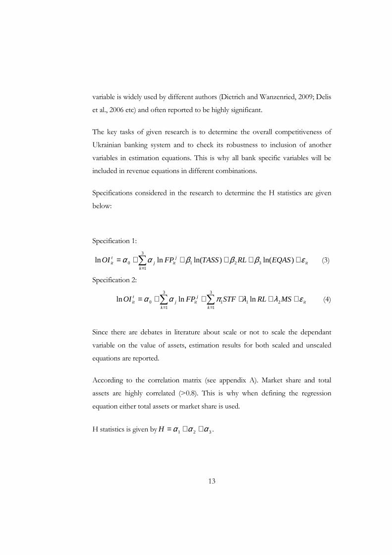
Specifications considered in the research to determine the H statistics are given

below:

Specification 1:

∑=

+++++=3

13210 )ln()ln(lnln

kit

jitj

tit EQASRLTASSFPOI εβββαα (3)

Specification 2:

∑ ∑= =

+++++=3

121

3

110 lnlnln

kit

k

jitj

tit MSRLSTFFPOI ελλπαα (4)

Since there are debates in literature about scale or not to scale the dependant

variable on the value of assets, estimation results for both scaled and unscaled

equations are reported.

According to the correlation matrix (see appendix A). Market share and total

assets are highly correlated (>0.8). This is why when defining the regression

equation either total assets or market share is used.

H statistics is given by 321 ααα ++=H .

14

Since there are two specifications used in the study, one needs corresponding two

specifications for testing the long-term equilibrium (E). Specification (5) for

testing the latter assumption for equation (3) and specification (6) for testing

whether assumption holds for equation (4):

∑=

+++++=+3

13210 )ln()ln(ln)1ln(

kit

jitj

tit EQASRLTASSFPROAA εβββϕα (5)

∑ ∑= =

+++++=+3

121

3

110 lnln)1ln(

kit

k

jitj

tit MSRLSTFFPROAA ελλπϕα (6)

where: ROA – return on assets.

E statistics defined as: 321 ϕϕϕ ++=E .

To estimate equations (3)-(6) the fixed and random effect estimation are used.

Various specification tests are to be applied to determine the best fit model.

Error term is assumed to be:

itiit eu +=ε (7)

According to Wooldridge (2003) simple regression may suffer from

omitted variable (efficiency of management, bank’s access to funding etc) bias –

this is the key reason for using the fixed effects estimator. The variable

iu captures all unobserved, time-constant factors that affect dependant variable.

The fixed effect estimator is robust to possible correlation of ui with other

explicative variables.

15

C h a p t e r 4

DATA DESCRIPTION

Data were collected primarily from the two sources: NBU and Association of

Ukrainian banks websites. The period is covered by the panel quarterly data

ranges from 2005:1 to 2009:1 inclusively and consists of 4 observations per each

year (quarterly data) reported in: January, April, July, October. The choice of

period for research is based on data availability. Because mostly variables used in

regression were not directly given, some deductions and ratios were made in

order to obtain all necessary variables for regression.

The main bank-by-bank dataset may be divided by four blocks:

• Assets. Given block enabled the research with the key scale variable –

assets per se. In addition, block allows to calculate the proxy for risk –

loans to assets ratio and market share of particular bank.

• Financial results. Contain the information about all kinds of expenses

which together with other blocks allow calculating the proxy for labor

expenses (factor price 2) and proxy for capital expenses (factor price 3),

operational income, return on assets. Unfortunately, given block stops

reporting the “personnel expenses” after 2009:1. The latter fact makes

impossible to expand research to further periods.

• Liabilities. This block together with “assets” allows to determine the

price of attracted funds (factor price 1). Also statistics concerning the

owners of deposits is reported (physical vs juridical person).

16

• Equity. Main variables contained within given block are statutory fund

dummies, which are reported in UAH. So, statutory fund in EUR in

particular quarter was found by converting the UAH into EUR using the

exchange rate prevailing at the same quarter. Reported equity column

allows to calculate the equity to assets ratio.

Reliability of data for some banks has been crosschecked by comparing the data

reported on the NBU website and those available at bank’s website. The sample

of about 40 % of banks has been taken in different points of time. Large

discrepancies were not observed since every rational bank understands that biased

information may lead to the loss of already obtained clients’ credence. Besides,

according to the information of website by Financial Initiative bank, Ukrainian

banks keep working at their openness. To illustrate this, “from 107 banks

included in the rating, 22 received the highest credibility category, 59 showed

acceptable credibility level and 26 financial institutions were assigned satisfactory

credibility level” (Financial Initiative, 2008). Thus, the major part of banks is quite

reliable (at least starting from 2005), which makes Ukrainian statistics useful. All

sites mentioned above have the data from which it is possible to calculate all

explicative and endogenous variables for equations (3) - (6).

Except for the Panzar-Rosse (1987) approach, there are also exist less advanced

methodologies for determining the level of competition in particular industry,

namely, the concentration ratio (CR) and Herfindahl-Hirschman Index (HHI).

The concentration ratio is the sum of market shares (MS) of m largest banks (3, 5

and 10 are the most widely used) calculated as the ratio of bank’s i assets and total

17

amount of all banks’ assets; assets are defined as the proxy for bank activity2. The

HHI is calculated as the sum of squared market shares of all industry participants.

Figures 4.1 and 4.2 contain the concentrations ratios for loans and assets

respectively. Empirically CR3 and CR5 for loans declined by January, 2009

comparing to January, 2005, may be because of increased quantity of banks (160

vs. 179), whereas the CR10 increased within the given period. That is, loans

concentration ratios yield ambiguous results depending on the number of banks

m used.

0

10

20

30

40

50

60

CR3 CR5 CR10

2005 loans

2009 loans

Figure 4.1. Concentration ratios for loans, %

Concentration ratios in terms of assets (figure 4.2) show similar results to loans:

decrease in CR3 and CR5, and negligible changes in CR10. This may be explained

by the fact that top 10 banks (in terms of assets) are different in 2005 and 2009

and during the wave of mergers and acquisitions of Ukrainian banks, foreign

banks had an opportunity to become top 10 banks. Although high concentration

ratio does not necessarily imply that market faces imperfect competition, but the

2 Alternatively in order to make proxy for bank activity more narrow loans or deposits may be used instead of

assets.

18

fact that 5 % (10 banks) are owners of 50 % of loans and assets puts a question

mark on the degree of competitiveness of Ukrainian banking sector.

0

10

20

30

40

50

60

CR3 CR5 CR10

2005 Assets

2009 Assets

Figure 4.2. Concentration ratios for assets, %

Looking at figure 4.3 one can see that HHI declines in January, 2009 comparing

to January, 2005. In spite of fluctuations HHI during the whole period indicates

an unconcentrated index which is consistent with competitive market.

340

360

380

400

420

HHI

2005q1 2006q1 2007q1 2008q1 2009q1period

Figure 4.3. HHI during 2005-2009

19

However, Claessens and Laeven (2004) and Bikker (2003) shown that

concentration ratios and HHI are poor measures of competition, because

industry may have high concentration ratios whereas the overall level of

competition is quite high. In given paper more advanced methodology is used

developed by Panzar and Rosse in order to obtain the unambiguous results

concerning the degree of competition of Ukrainian banks. To estimate the degree

of competition regression equations (3) and (4) include three factor prices

variables defined in the methodology section and bank-specific variables to

control for different size of banks and risks.

Descriptive statistics for all variables necessary for estimation of equations (3), (4)

is presented in table 4.1. It contains the aggregated statistics over the whole

period 2005:1-2009:1. Worth mentioning that, the total number of observations is

2861 (see appendix for descriptive statistics of the whole population). However,

due to the log-log specification of estimated equations and unbalanced panel data,

negative values of operational income were dropped (91 observations). That is,

regression sample represents about 97 % of initial population (2770 vs 2861),

which makes sample data quite reliable.

Table 4.1. Sample summary statistics over the whole period

Variable Obs Mean Std. Dev. Min Max

Opertional income, mil UAH

2770 122.54 409.68 0.06 9844.54

ROA, ratio 2770 0.01 0.02 -0.45 0.23

Interest revenue/deposits and equivalents (FP1), ratio

2770 0.05 0.04 0.00 1.30

20

Table 4.1 – Continued

Variable Obs Mean Std. Dev. Min Max

Personnel expenses/total assets (FP2), ratio 2770 0.02 0.01 0.00 0.23

Non-personnel expenses/total assets (FP3), ratio

2770 0.02 0.01 0.00 0.22

loans/assets (RL), ratio 2770 0.66 0.25 0.02 11.25

total assets (TASS), mil UAH

2770 2471.93 6474.24 24.21 80200.00

equity/assets (EQAS), ratio

2770 0.22 0.18 0.00 2.24

market share (MS), % 2770 0.61 1.39 0.01 11.11

Statutory fund dummies

statutory fund (small banks), mil euro 72 2488.51 378.87 1744.38 2988.51

statutory fund (medium banks), mil euro

468 4103.18 564.77 3006.66 4995.33

statutory fund (big banks), mil euro

2230 31090.77 63801.47 5000 1280369

Looking at table 4.1 one can deduce that in spite of the quite high operational

income the return on asset in banking sector is quite low (on average 1 %). This

may be explained by the high value of total assets (average value about 3 billion

UAH). Loans to assets ratio varies a lot from 0.02 to 11.25 multiple. Worth

mentioning that most part of Ukrainian banks are big banks with statutory fund

higher than 5 000 000 euro.

21

C h a p t e r 5

ESTIMATION RESULTS

Estimation results for both specifications (3), (4) are reported in Appendix C.

Since there are two different specifications which use both scaled and unscaled

operational income, the total number of regression equation totals to four.

Equations in Appendix C do not control for time specific intercept. In contrast,

Appendix E contains obtained results for the same specifications, but controlling

for time-specific intercept and Appendix F reports the long-run equilibrium test

when controlling for time specific intercept.

Let’s consider equations without time dummies first (Appendix C). From

estimated results it may be concluded that all factor prices are significant at 1 %

confidence interval. In given case, in spite of different value of H statistics (ranges

from 0.94 to 0.99) the main conclusion is not changed: Ukrainian banking system

faces the intermediate case of competition (between monopolistic and perfect) in

which an increase in costs causes operational income to increase at a rate slower

than the rate of increase in costs. Obtained estimates of H statistics are robust to

inclusion of other explicative variables (since all specifications yield similar value

of H), in spite of difference in values of estimates near the factor prices. In spite

of the fact that, the value of H statistics is very close to 1 the F-test rejects the

hypothesis that H=1 (H=0 is rejected either) 1 % confidence interval in three out

of four different specifications (see Appendix C).

As an alternative to fixed effect one could use the random effect estimation.

However, the random effect model is rejected by Hausman and Breusch-Pagan

tests. Thus, that variation of bank-specific unobservables across banks is not

22

random, but constant over time and correlated with the independent variables

included in the model.

From looking at estimate results it may be concluded that rise in total assets by

1 % increases the operational income by 1.05 % (economy of scale) and

operational income/asset ratio by .05 %, which is consistent with the difference

in models’ specifications.

Estimation results suggest that ratio of loans to assets has the significant impact

on the dependant variable although its value changes as the specification of the

model changes. On average increase in the loans/assets ratio by 1 % causes

operational income to increase by 0.2-0.5 % (depending on the specification of

model) and operational income to assets ratio by 0.2 %. Thus, in any case,

Ukrainian banking loan market remunerates for risk.

Dummy variables reflecting the size of statutory capital are quite ambiguous and

depend on the model specification. Market share has unambiguously positive

significant impact on dependent variables despite of its specification.

Let’s switch to Appendix D where regressions coefficients are reported, but

controlling for time specific intercept. Depending on the specification the value

of H statistics varies from 0.11 to 0.62, indicating mush higher variation

comparing to the specifications which did not control for time specific intercept.

Nevertheless, since the value of H statistics lies in the interval between 0 and 1

for all specifications, the conclusion about monopolistic competition in Ukrainian

banking sector is still valid and confirms the results of regressions obtained

without control for time specific intercept (Appendix C). Concerning the bank

specific variables one can deduce that total assets and equity to assets ratio have

positive and significant impact on operational income disregarding the scaling.

However, the market share positively and significantly impacts operational

23

income only in specification with unscaled dependant variable (operational

income per se).

Thus, two sets of models presenting the same conclusions concerning the market

structure of the market (monopolistic competition). In order to choose the best

one needs to refer to the assumption of long-run equilibrium, according to which

the profitability of banks should not be statistically correlated with factor prices.

For doing the dependant variable in both specifications is replaced by the return

on assets (ROA) and regressed against all explicative variables considered in

particular specifications (equations (5), (6)). According to Matousek et al. (2009)

at competitive markets the return is uniform across the banks. That is, bank’s

operational income should not be correlated statistically with the rate of return

(E=0). Table C2 contains the value of E statistics for specification without period

dummies in which F test rejects the hypothesis that E=0 since the p-value is 0. In

contrast, from Table D2 it follows that for specification 1 the hypothesis that

E=0 can not be rejected at even 10 % confidence interval, whereas the E

statistics for specification 2 may be rejected at 10 % confidence interval. In any

case, when controlling for time-specific intercept the assumption about long-run

equilibrium is more likely to hold comparing to models without time dummies

(Appendix C).

To conclude, it was found that controlling for time dummies imply that

assumption about long run equilibrium holds. In such a way, it is deduced that

Ukrainian banking sector faces the monopolistic competition since estimated

value of H statistics ranges from 0.11 to 0.62. The hypotheses about pure

monopoly and perfect competition are strongly rejected.

24

C h a p t e r 6

CONCLUSIONS

In given paper the Panzar-Rosse (1987) approach is used to estimate the degree

of competition of Ukrainian banking sector. Instead of focusing on some

particular bank’s activity (loan or deposits market), this methodology tests the

level of competitiveness over bank’s activities, since the total operational income

is used as a dependant variable. From estimated results it may be deduced that

purely theoretical formulation of H statistics is consistent with bank’s conduct in

the case of Ukraine; given methodology proved itself to be quite reliable and

widely used in modern literature. Panzar-Rosse methodology assigns a particular

numerical value which is the basis for the conclusion about the dominant market

structure in the industry.

Banks play the vital role in economy through payment system functioning,

redistribution of wealth through attracting deposits and giving loans etc.

Moreover, there are certain papers which prove that economic growth of the

country is linked to the development of banking system (Strahan, 1996; Levine,

2003). The crucial role of banks in country’s growth makes the issue of

competition extremely important. Since, the inevitable consequence of

competition is the reduction of prices charged by banks for their services which

positively impacts the welfare of consumers.

In paper different specifications are used to see whether factor prices coefficients

are robust to inclusion of different variables. Regressions which contain the time-

specific intercept tend to be more reliable comparing to models with common

intercept, since time dummies insure that long-run equilibrium assumption holds.

25

Concerning the estimated value of H statistics, it varies between 0.11 and 0.62

(controlling for time-specific intercept). In spite of fluctuations, the main

conclusion of a paper is common for all specifications: Ukrainian banks earn their

profits in market with monopolistic competition, which is far from perfect3. The

hypothesis about perfect monopoly is strongly rejected for all specifications.

However, there is still place for improvement towards the perfect competition.

Concerning the bank specific variables, total assets have positive and significant

impact on both scaled and unscaled operational income. Loans to assets ratio

indicates that market remunerates for risk – higher values of operational income

are associated with proxy for risk. Equity positively and significantly impacts

operational income, whereas the market share has ambiguous impact on income.

From the theoretical point of view the estimated value of H statistics indicate that

average consumer overpays for bank services comparing to perfect competition

situation. Governors are also worse off since the competitive markets are easier

to regulate through market mechanisms, whereas the monopolistic competition

requires directive policy methods.

As an extension of given paper one could extrapolate the given methodology for

determining the level of competition in other industries. This would help policy

makers to apply the most appropriate mechanism for regulations (market or

administrative mechanism).

3 Although models with common intercept suggest the value of H at the level of 0.98. The assumption about

long-run equilibrium fails, since the value of E is not equal to zero statistically.

26

WORKS CITED

Bikker, J. A. 2003. Testing for Imperfect Competition on EU Deposit and Loan Markets

with Bresnahan's Market Power Model. Kredit und Kapital, 2, 167-212.

Bikker, J. A. and K. Haaf. 2002. Competition, concentration and their relationship: An

empirical analysis of the banking industry. Journal of Banking & Finance 26 (2002),

2191-2214.

Bikker, J. A., S. Shaffer and L. Spierdijk. 2009. The Panzar-Rosse Revenue Test: To

Scale or Not to Scale? Working paper

Boone, J. 2008. A new way to measure competition. Economic Journal, Vol. 118,

1245-1261, 2008.

Boot A., and A.V. Thakor. 2000. Can the relationship banking survive competition? The

Journal of finance, Vol. LV, NO.2.

Breshahan, T. F. 1982. The oligopoly solution concept is identified. Economics Letters,

10, pp. 87-92.

Casu, B., and C. Girardone. 2009. Bank Competition, Concentration and Efficiency in the

Single European Market. Working paper.

Cetorelli N. 2001. Competition among banks: Good or bad? Federal Reserve Bank of

Chicago. Working paper.

Claessens S., L. Laeven. 2003. What Drives Bank Competition? Some International

Evidence. The World Bank Financial Sector Operations and Policy Department,

2003.

27

Dietrich, A., and G. Wanzenried. 2009. What determines the profitability of commercial

banks? New evidence from Switzerland.

Financial Initiative. 2008. “News”. www.the-bank.com.ua

Gischer H., and M. Stiele. 2003. Testing for Banking Competition in Germany: Evidence

from Savings Banks. Working paper.

Golodniuk, I. 2006. Evidence on the Bank Lending Channel in Ukraine. Research in

International Business and Finance, Volume 20/2.

Hempell, H.S. 2002. Testing for Competition Among German Banks. Discussion

paper 04/02 Economic Research Centre of the Deutsche Bundesbank.

Leuvensteijn, M., J.A. Bikker, A. Rixtel, and C. Kok-Sorensen. 2007. A New

Approach to Measuring Competition in the Loan Markets of the Euro Area. Working

paper.

Levine, Ross. 2003. More on Finance and Growth: More Finance, More Growth? Federal

Reserve Bank of St. Louis Review, July/August 2003, 85(4), pp. 31-46

Maslovych M. 2009. The Boone Indicator as a Measure of Competition in Banking Sector:

the case of Ukraine. EERC thesis.

Matousek, R., S. Minegishi, and C. Stewart. 2009. Competitiveness of Credit

Associations and Credit Cooperatives in Japan. Discussion paper.

Panzar, J.C., and J. N. Rosse. 1987. “Testing for “Monopoly Equilibrium”.

Journal of Industrial Economics, 35, 4, 443-456.

28

Pasiouras F., and K. Kosmidou. 2007. Factors influencing the profitability of domestic and

foreign commercial banks in the European Union. Research in International Business

and Finance 21 (2007) 222–237.

Schaek K., M. Cihak. 2008. How does the competition affect efficiency and soundness in

banking? New empirical evidence. Working paper

Sealey, C.W. and J. T. Lindley. 1977. Inputs, Outputs, and Theory of Production Cost at

Depository Financial Institutions. Journal of Finance 32, 1251-1266.

Segura, E. 2010. Banking/Financial Crises and Financial Sector Reform. Lecture notes

Shaffer, S. 1994. Conduct in a Banking Duopoly. Journal of Banking and Finance 18.

Talavera, O. et al. 2006. Macroeconomic Uncertainty and Bank Lending: The Case of

Ukraine. Discussion Papers of DIW Berlin 637, DIW Berlin, German Institute

for Economic Research.

Thakor A.V., and A.W. Boot. 2008. Handbook of financial intermediation and banking.

Vol.1, p. 6-10.

Turchynska K.. 2005. Bank mergers and acquisitions in Ukraine: efficiency effects and

implications. EERC thesis.

Ukrainian Banks Assosiation. 2002. “Activity of Banks”

http://www.aub.com.ua/

APPENDIX A

Table A1: Correlation matrix of regression sample

Operational income

Factor price 1

Factor price 2

Factor price 3

Total assets

Loans/Assets, ratio

Equity/Assets, ratio

Market share, %

Return on assets, ratio

Operational income 1.00 Factor price 1 0.02 1.00 Factor price 2 0.07 0.33 1.00 Factor price 3 0.01 0.37 0.76 1.00 Total assets 0.89 -0.05 -0.04 -0.11 1.00

Loans/Assets, ratio 0.10 0.07 0.10 0.09 0.10 1.00

Equity/Assets, ratio -0.17 0.06 0.17 0.24 -0.23 0.08 1.00 Market share, % 0.72 -0.07 -0.05 -0.09 0.84 0.08 -0.26 1.00

Return on assets, ratio 0.05 0.04 -0.14 -0.17 0.03 0.03 -0.04 0.03 1.00

29

30

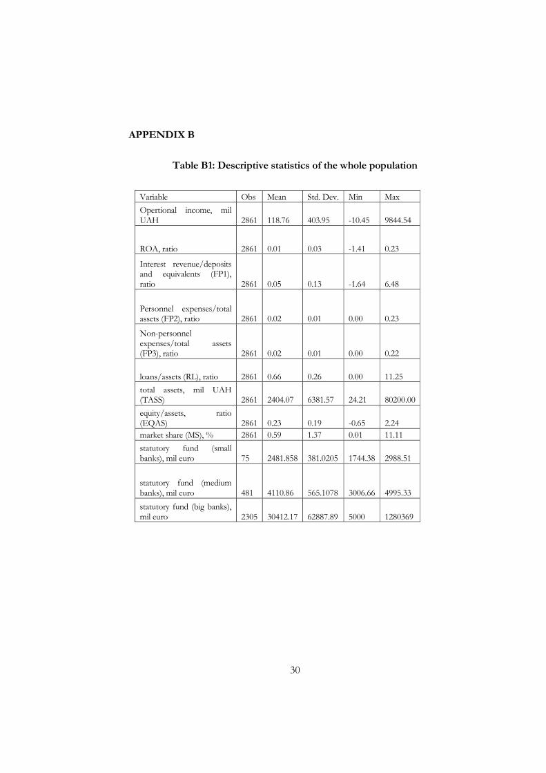
APPENDIX B

Table B1: Descriptive statistics of the whole population

Variable Obs Mean Std. Dev. Min Max

Opertional income, mil UAH 2861 118.76 403.95 -10.45 9844.54

ROA, ratio 2861 0.01 0.03 -1.41 0.23

Interest revenue/deposits and equivalents (FP1), ratio 2861 0.05 0.13 -1.64 6.48

Personnel expenses/total assets (FP2), ratio 2861 0.02 0.01 0.00 0.23

Non-personnel expenses/total assets (FP3), ratio 2861 0.02 0.01 0.00 0.22

loans/assets (RL), ratio 2861 0.66 0.26 0.00 11.25

total assets, mil UAH (TASS) 2861 2404.07 6381.57 24.21 80200.00

equity/assets, ratio (EQAS) 2861 0.23 0.19 -0.65 2.24 market share (MS), % 2861 0.59 1.37 0.01 11.11

statutory fund (small banks), mil euro 75 2481.858 381.0205 1744.38 2988.51

statutory fund (medium banks), mil euro 481 4110.86 565.1078 3006.66 4995.33

statutory fund (big banks), mil euro 2305 30412.17 62887.89 5000 1280369

31

APPENDIX C

Table C1: Estimation results for regression equations (3) and (4)

Specification 1 Specification 2 Dependant variable LN(OI) LN(OI/ASSETS) LN(OI) LN(OI/ASSETS)

log of FP1 0.134 (0.031)**

0.134 (0.031)**

0.523 (0.060)**

0.151 (0.033)**

log of FP2 0.294 (0.033)**

0.294 (0.033)**

0.736 (0.058)**

0.341 (0.032)**

log of FP3 0.512 (0.025)**

0.512 (0.025)**

-0.274 (0.053)**

0.464 (0.026)**

log of Total Assets

1.051 (0.012)**

0.051 (0.012)** - -

log of Loans/Assets

0.177 (0.037)**

0.177 (0.037)**

0.429 (0.085)**

0.189 (0.038)**

log of Equity/Assets

0.022 (0.005)**

0.022 (0.005)** - -

small banks - - -0.62 (0.082)**

0.068 -0.037

midle banks - - -0.314 (0.045)**

0.067 (0.022)**

market share - - 0.676 (0.104)**

0.072 (0.020)**

Constant 0.215 -0.19

0.215 -0.19

13.832 (0.125)**

0.866 (0.064)**

Observations 2770 2770 2770 2770 H stats (logFP1+logFP2+logFP3) 0.94 0.94 0.985 0.956 F test that ∑FP=1, p-value 0 0 0.52 0 Number of unique_id 212 212 212 212 R-squared 0.9 0.81 0.54 0.81

Robust standard errors in parentheses

* significant at 5%; ** significant at 1%

32

Table C2: Long-run equilibrium test for regression equations (3) and (4)

Specification 1 Specification 2 Dependant variable ln(ROA)

log of FP1 0.006 (0.004)

0.007 (0.005)

log of FP2 -0.004 (0.004)

-0.003 (0.003)

log of FP3 0 (0.002)

-0.001 (0.002)

log of Loans/Assets 0.005 (0.004)

0.006 (0.004)

log of Total Assets 0.002 0.001 -

log of Equity/Assets 0 0 -

small banks - 0.004 (0.002)*

midle banks - 0.002 (0.001)

market share - 0 (0.001)

Constant -0.008 (0.022)

0.014 (0.008)

Observations 2770 2770 E stats (logFP1+logFP2+logFP3) 0.002 0.003 F test that ∑FP=0, p-value 0 0 Number of unique_id 212 212 R-squared 0.05 0.05

Robust standard errors in parentheses

* significant at 5%; ** significant at 1%

33

APPENDIX D

Table D1: Estimation results for regression equations (3) and (4)4

Specification 1 Specification 2

Dependant variable LN(OI) LN(OI/ASSETS) LN(OI) LN(OI/ASSETS)

log of FP1 0.06 (0.030)*

0.06 (0.030)*

0.197 (0.046)**

0.073 (0.032)*

log of FP2 0.27 (0.032)**

0.27 (0.032)**

-0.191 (0.048)**

0.228 (0.033)**

log of FP3 0.286 (0.037)**

0.286 (0.037)**

0.102 -0.054

0.272 (0.037)**

log of Loans/Assets 0.301 (0.039)**

0.301 (0.039)**

0.487 (0.067)**

0.316 (0.040)**

log of Total Assets 1.104 (0.029)**

0.104 (0.029)** - -

log of Equity/Assets 0.03 (0.009)**

0.03 (0.009)** - -

small banks - - -0.008 (-0.061)

0.024 (-0.037)

midle banks - - -0.009 (-0.029)

0.048 (0.021)*

market share - - 0.497 (0.058)**

-0.007 (0.019)

Constant -1.337 (0.327)**

-1.337 (0.327)**

10.161 (0.230)**

-0.274 (0.167)

Observations 2770 2770 2770 2770 H stats (logFP1+logFP2+logFP3) 0.616 0.616 0.108 0.573 F test that ∑FP=1, p-value 0 0 0 0 Number of unique_id 212 212 212 212 R-squared 0.92 0.84 0.82 0.84

Robust standard errors in parentheses

* significant at 5%; ** significant at 1%

4 All four specifications in Table D1 control for time specific intercept.

34

Table D2: Long-run equilibrium test for regression equations (3) and (4)5

Specification 1 Specification 2 Dependant variable ln(ROA)

log of FP1 0.004 (0.004)

0.005 (0.004)

log of FP2 -0.001 (0.003)

-0.004 (0.004)

log of FP3 -0.006 (0.003)*

-0.007 (0.003)*

log of Loans/Assets 0.008 (0.004)*

0.01 (0.004)*

log of Total Assets 0.008 (0.003)** -

log of Equity/Assets 0.001 (0.001) -

small banks - 0.002 (0.002)

midle banks - 0.001 (0.001)

ms - -0.001 (0.001)

Constant -0.094 (0.042)*

-0.012 (0.016)

Observations 2770 2770 E stats (logFP1+logFP2+logFP3) 0.00 -0.01 F test that ∑FP=0, p-value 0.27 0.07 Number of unique_id 212 212 R-squared 0.09 0.08

Robust standard errors in parentheses

* significant at 5%; ** significant at 1%

5 All four specifications in Table D2 control for time specific intercept