Testing Factor Models

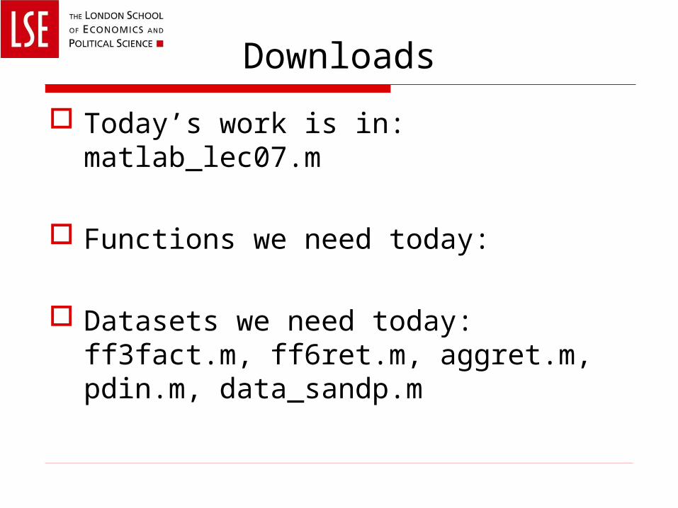
Downloads

Today’s work is in: matlab_lec07.m

Functions we need today:

Datasets we need today: ff3fact.m, ff6ret.m, aggret.m, pdin.m, data_sandp.m

Factor Models

Suppose factors are good proxies for risk Suppose factors are uncorrelated Suppose factors themselves can be represented by

excess returns (ie Rm-Rf or Ri-Rk) E[Ri-Rk]=B1

iE[F1]+B2iE[F2]+… +εit where

B1i=Cov[Ri-Rk,F1]/Var[F1] …

This implies that in a regression: Rit-Rft=αi+β1

iF1t+β2

iF2t+εit and αi=0 for all assets!

(this part does not need factors to be uncorrelated) If α≠0 for some asset, either (1) This is model does

not do a good job or (2) This asset, for some reason, has an abnormal return

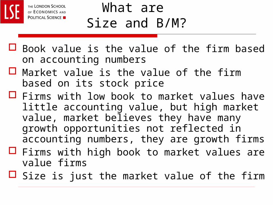
What are Size and B/M?

Book value is the value of the firm based on accounting numbers

Market value is the value of the firm based on its stock price

Firms with low book to market values have little accounting value, but high market value, market believes they have many growth opportunities not reflected in accounting numbers, they are growth firms

Firms with high book to market values are value firms

Size is just the market value of the firm

SortingPortfolios

Fama and French calculate each firm’s size and B/M each year and then sort them according to those quantities

This is called a double sort They then create 6 portfolios (3x2), ie (highest

B/M+lowest size), (middle B/M+highest size), etc They calculate each portfolio’s return for one year Next year they resort and form new portfolios This is a strategy that a market participant (ie

mutual fund) could follow as well

FF factors

They use the sorted portfolios to create new, long/short portfolios

SMB (small minus big) goes long in the small portfolio, and finances this by going short in the large portfolio, its return is RS-RB

HML (high minus low) goes long in the high B/M (value) portfolio, and finances this by going short in the low B/M (growth) portfolio, its return is RB-RL

Note, these are zero cost portfolios, other than transaction costs, these portfolios cost you nothing

Download Returns and Factors

Load the files ff3fact.m and ff6ret.m into Matlab Alternately, save files into your matlab directory

and type their names into the matlab prompt This data comes from Kenneth French’s website:

http://mba.tuck.dartmouth.edu/pages/faculty/ken.french/data_library.html

% Small Big % Low 2 High Low 2 High >>disp(mean(FF6ret(:,2:7))); 1.0234 1.3215 1.5255 0.9237 1.0125 1.2404% Mkt-RF SMB HML RF>>disp(mean(FFfactors(:,2:5))); 0.6511 0.2314 0.4097 0.3064

What is Risk?

Small and Value stocks have higher average returns, does this imply market is inefficient? No!

They should have higher average returns, if they are more risky? Are they more risky? What is risk?

Assets that covary with aggregate risk are more risky. What is aggregate risk?

CAPM says the market return is a proxy for aggregate risk

Test CAPM on FF6

The CAPM says that the average return on any asset (or portfolio of assets) should depend on the covariance of that asset (or portfolio) with the market return

E[R-Rf]=[Cov(R,Rm)/Var(Rm)]*E[Rm-Rf] Think back to the definition of regression: if we

regress Rt-Rtf=α+β*(Rt

m-Rtf)+εt, then

β=[Cov(R-Rf,Rm-Rf)/Var(RmRf)]=[Cov(R,Rm)/Var(Rm)] and α=E[R-Rf]-B*E[Rm-Rf] Thus, CAPM predicts α=0 for each asset

Test CAPM on FF6

>>[T w]=size(FFfactors);>>X=[ones(T,1) FFfactors(:,2)];>>for i=1:6; Y=FF6ret(:,1+i)-FFfactors(:,5); [regcoef sterr]=regress(Y,X); outcapm(i,:)=[regcoef(1) sterr(1,1) sterr(1,2)]; end;>>disp(outcapm);>>plot(mean(FF6ret(:,2:7)),mean(FF6ret(:,2:7)),'k-');>>hold on;>>plot(mean(FF6ret(:,2:7)), mean(FF6ret(:,2:7))-outcapm(:,1)','b.');

Predicted vs actual

Test FF 3 factor

A multifactor model is similar to a one factor model

FF 3-Factor Model suggests market is not the only source of risk, SMB and HML also proxy for risk

The regression Rt-Rt

f=α+β1*(Rtm-Rt

f)+β2*SMBt+β3*HMLt +εt

should have α=0 for each asset Note that the factors are all excess returns, so

this conforms to definition in first slide F1=Rm-Rf, F2=RS-RB, F3=RH-RL

Test FF 3 factor

>>[T w]=size(FFfactors);>>X=[ones(T,1) FFfactors(:,2:4)];>>for i=1:6; Y=FF6ret(:,1+i)-FFfactors(:,5); [regcoef sterr]=regress(Y,X); out3f(i,:)=[regcoef(1) sterr(1,1) sterr(1,2)]; end;>>disp(outcapm);>>plot(mean(FF6ret(:,2:7)),mean(FF6ret(:,2:7)),'k-');>>hold on;>>plot(mean(FF6ret(:,2:7)), mean(FF6ret(:,2:7))-out3f(:,1)','rx');

Predictedvs actual

Return Predictability

Returns seem to be weakly predictable The predictability becomes stronger when we

aggregate returns over longer horizons Several variables have predictive power, among

these are P/D, P/E, cay, long-term component of consumption growth

This does not necessarily violate EMH For example, expected returns may be higher

during recessions, but these are also times when investors face the most risk, and when they are most likely to be constrained

Getting P/D data (optional)

From CRSP get the Market, Value Weighted Return, including distributions, and excluding dividends for 1926-2008

Since you need to enter the name of a security, use GE (it existed for all those years)

This is used to make the dataset aggret.m (on my website). This dataset contains return (including dividends) in the 3rd column, and return (excluding dividends) in the 4th column. Load this into matlab

>>[T b]=size(aggreturn);>>price(1)=1; dividend(1)=0;>>for t=2:T; timeline(t)=round(aggreturn(t,2)/10000); price(t)=price(t-1)*(aggreturn(t,4)+1); %calculate price of firm next year using the ex-dividend return dividend(t)=price(t-1)*(aggreturn(t,3)+1)-price(t); %calculate dividend by subtracting ex-dividend price from %cum-dividend price end; dividend(1)=dividend(2); %use some number other than zero This creates a monthly time series for prices (Jan 1926 normalized to 1)

and dividends

DownloadPredictors

Load the data from pdin.m on my website>>pdin; matrix called pddata (996x5), contains monthly data for

Jan 1926-Dec 2006 Its columns are date, price (normalized to Jan 1926 being

1), dividend, price/dividend, aggregate return Gordon Growth Model: P/D high implies prices are high

relative to payouts, so high growth expected>>subplot(2,1,1); plot(pddata(:,5));>>in=1:12:T; >>subplot(2,1,2);

plot(round(pddata(in,1)/10000),pddata(in,4)); Note that P/D has increased over the period, have

distributions changed so dramatically? P/E is a better measure, firms are paying less dividends,

but investors are getting paid in other ways

Monthly Predictability

In practice want to use most recent data In historical analysis, use extra lags to make

sure you are not using contemporaneous information

>>[T a]=size(pddata);>>Y=pddata(7:T,5); >>X=[ones(T-6,1) pddata(1:T-6,4)/12];>>[regcoef sterr a3 a4 rsq]=regress(Y,X);>>disp([regcoef sterr]); disp(rsq(1)); Regression coefficient is negative (high prices

today lead to low returns in future), but not significant

R2 is very small

Annual Predictability

What if we try to predict the cumulative annual return rather than just a monthly return?

Calculate cumulative annual return for year t, regress it on the P/D ratio in July of t-1

>>T1=floor(T/12); %number of years in our data>>for i=2:T1; in=(i-1)*12+1:(i-1)*12+12; %selective index for year i Y(i,1)=sum(pddata(in,5)); X(i,1)=1; X(i,2)=pddata((i-1)*12+1-7,4); end;>>[regcoef sterr a3 a4 rsq]=regress(Y(2:T1),X(2:T1,:));>>disp([regcoef sterr]); disp(rsq(1)); R2=7.3%, annual returns over this period are predicted by

P/D!

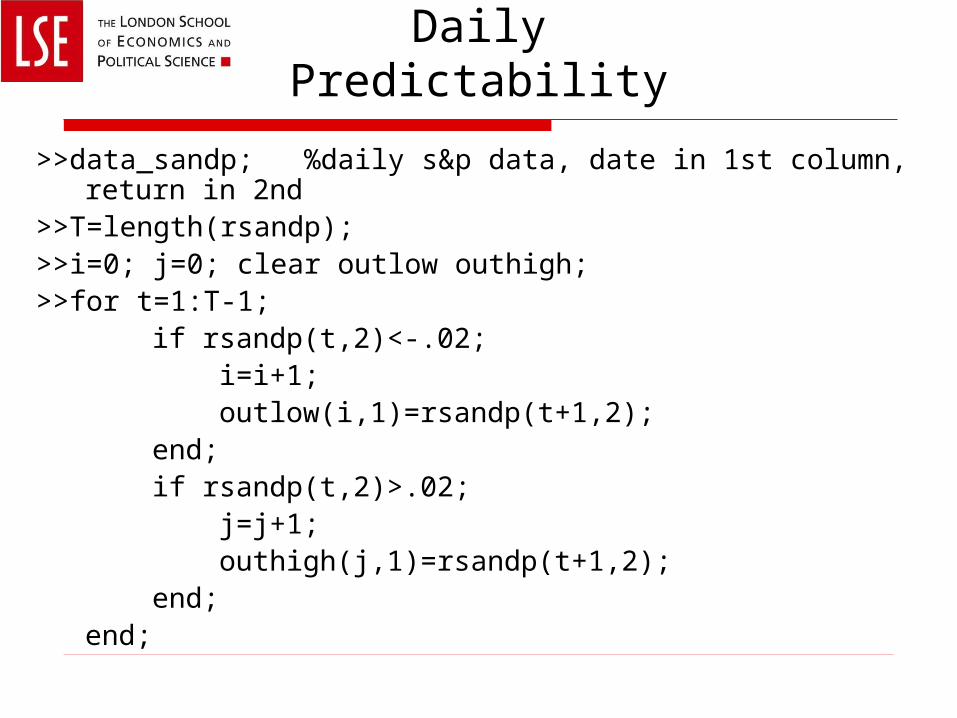
DailyPredictability

Technical Analysis: Claims the ability to forecast the future direction of stock prices through the study of past market data, primarily price and volume.

“I realized technical analysis didn't work when I turned the charts upside down and didn't get a different answer” Warren Buffet

“Market really went down [up] today, I bet its going up [down] tomorrow!” My dad

DailyPredictability

>>data_sandp; %daily s&p data, date in 1st column, return in 2nd

>>T=length(rsandp);>>i=0; j=0; clear outlow outhigh;>>for t=1:T-1;

if rsandp(t,2)<-.02; i=i+1; outlow(i,1)=rsandp(t+1,2); end; if rsandp(t,2)>.02; j=j+1; outhigh(j,1)=rsandp(t+1,2); end;end;

DailyPredictability

>>disp([mean(rsandp(:,2)) mean(outlow) mean(outhigh) std(outlow) std(outhigh)]);

0.0003 0.0004 0.0033 0.0226 0.0134

>>rmin=min(rsandp(:,2));>>rmax=max(rsandp(:,2));>>subplot(2,1,1);>>hist(outlow,[rmin:.01:rmax]); >>subplot(2,1,2);>>hist(outhigh,[rmin:.01:rmax]);

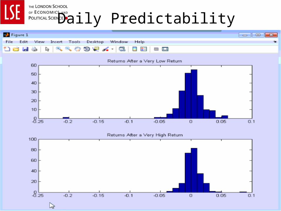
Daily Predictability