Testing dark energy and modified gravity modelswith EFTCAMB/EFTCosmoMC

Noemi Frusciante

Based onNF, Marco Raveri, Alessandra Silvestri, JCAP 1402 026 (2014) [arXiv:1310.6026]

Bin Hu, Marco Raveri, NF, Alessandra Silvestri, PRD 89 (2014) 103530 [arXiv:1312.5742]

Marco Raveri, Bin Hu, NF, Alessandra Silvestri, PRD 90 (2014) 043513 [arXiv:1405.1022]

Bin Hu, Marco Raveri, Alessandra Silvestri, NF, PRD 91 (2015) 063524 [arXiv:1410.5807]

EFTCAMB webpage : http://wwwhome.lorentz.leidenuniv.nl/ hu/codes/

Hot topics in Modern Cosmology - SW IX27 April - 1 May 2015, Cargese

Outline

• Motivation;

• Effective Field Theory for cosmic acceleration;

• Dynamical analysis of the background equations;

• EFTCAMB/EFTCosmoMC;

• Testing theory of gravity: examples.

State of the art of Modern Cosmology

• Two Unknown components:• Dark Energy: SNIa, CMB, BAO, Galaxy Cluster counts (68.3%)

⇓Recent accelerated expansion

• Dark Matter: flat RCs, BBN, CMB, Lensing, LSS (26.8%)⇓

Only Gravitational interaction, Non-Baryonic

• Homogeneous & Isotropic Universe;

• Spatially Flat Ωk ∼ 0;

⇓Dark Universe ∼ 95%

Best working model:

ΛCDM → GR + FLRW + Λ+CDM

Λ→ extra fluid : wΛ ≡ pΛ

ρΛ= −1

Deviations from General Relativity in Cosmology

Why do we need to Modify Gravity?

• Inflation: Fine tuning problems in theearly Universe;

• Late time accelerated expansion;

• Quantum Gravity;

• Dark Matter issues: Observations vsN-body simulations

Modifying General Relativity

How to modify GR:

• extra DoF(s): scalar, vector, tensor field(s);

• going beyond the 2nd order differential equations;

• diffeomorphism invariance breaking;

• higher than 4 dimensions;

In the following we will focus on theories with

• An extra scalar and dynamical DoF;

• Higher order field equations.

Solar system constraints

• Screening mechanisms(Chameleon, Symmetron, k-mouflage, Vainshtein)

Test gravity on cosmological scale

• Pletora of Dark Energy & Modified Gravity models• cosmological constant, quintessence, k-essence...• f(R), Brans-Dicke theories, Galileon.....

• Model independent parametrizations to test gravity on cosmologicalscale, to name (among others) the most recent• Growth functions: µ and γ,

[Silvestri et al. PRD 87, 104015 (2013)]

• Parametrized Post Friedmann framework,

[Baker et al., PRD 87, 024015 (2013)]

• Effective Field Theory of Cosmic Acceleration,

[Gubitosi et al. JCAP 1302 (2013) 032Bloomfield et al. JCAP 1308 (2013) 010]

• Horndeski parametrization,

[Bellini & Sawicki, JCAP 1407 (2014) 050]

Effective Field Theory Action• Operators are time-dependent spatial diffeomorphisms invariants;

• Unitary gauge: the extra scalar d.o.f. does not appear directly in theaction, i.e. scalar field perturbations are vanishing;

• Jordan frame: directly related to observations;

• Sm[χi , gµν ]: Validity of the Weak Equivalence Principle.

The action:

S =

∫d4x√−g

m2

0

2(1 + Ω(t)) R + Λ(t)− c(t)δg 00+

M42 (t)

2(δg 00)2

−M31 (t)

2δg 00δK − M2

3 (t)

2δKµ

ν δKνµ +

M2(t)

2δg 00δR(3)

−M22 (t)

2(δK )2 + m2

2(t)(gµν + nµnν)∂µg 00∂νg 00 + . . .

+ Sm[χi , gµν ]

where e.g. δA = A− A(0)

Stuckelberg Field & the extra dynamical scalar DoF

Stuckelberg technique: restoring the time diffeomorphism invariance byan infinitesimal time coordinate transformation

t → t + π(xµ).

Making manifest the extra scalar DoF will modify all the EFT functionswhich are typically Taylor expanded in π according to

f (t)→ f (t + π(xµ)) = f (t) + f (t)π +f (t)

2π2 + . . . .

Operators that are not fully diffeomorphism invariant transform accordingto the tensor transformation law, e.g.

g 00 → ∂(t + π(xµ))

∂xµ

∂(t + π(xµ))

∂xνgµν

= g 00 − 2π + 2πδg 00 − π2 − (∇π)2

a2+ ...

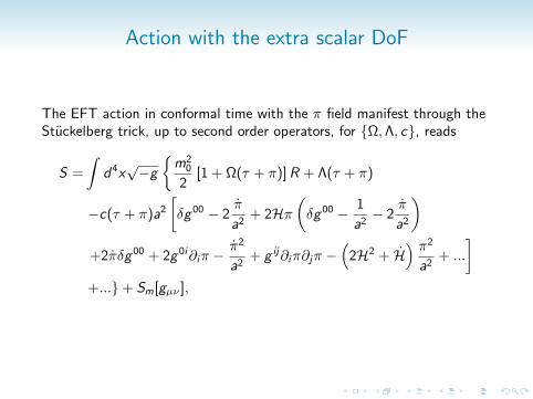
Action with the extra scalar DoF

The EFT action in conformal time with the π field manifest through theStuckelberg trick, up to second order operators, for Ω,Λ, c, reads

S =

∫d4x√−g

m2

0

2[1 + Ω(τ + π)] R + Λ(τ + π)

−c(τ + π)a2

[δg 00 − 2

π

a2+ 2Hπ

(δg 00 − 1

a2− 2

π

a2

)+2πδg 00 + 2g 0i∂iπ −

π2

a2+ g ij∂iπ∂jπ −

(2H2 + H

) π2

a2+ ...

]+...+ Sm[gµν ],

Advantages & Limitations

• Model independent framework to address the acceleration issue;

• Parametrization of DE/MG theories with a single extra scalar DoF ;

• The EFT functions are all unknown functions of time;

• Precise mapping between EFT functions and most of the singlescalar field DE/MG models.

• Low energy description of cosmological phenomena;

• Only single scalar field → No vector or tensor fields;

• Action does not describe higher-dimensional theories.

Examples of Mapping

• f(R)-theory:∫d4x

m20

2(R + f (R))→

∫d4x

m20

2[(1 + f ′0 ))) R + f0 − R0f ′0 ]

then

Ω(t) = f ′0 , Λ(t) =m2

0

2f0 − R0f ′0 , c(t) = 0

• Minimally coupled quintessence:

Sφ =∫

d4x√−g[

m20

2 R − 12∂

νφ∂νφ− V (φ)].

→∫

d4x√−g[

m20

2 R +φ2

0

2 δg 00 +φ2

0

2 − V (φ0)].

then

Ω(t) = 0, c(t) =φ2

0

2, Λ(t) =

φ20

2− V (φ0).

others:ΛCDM, non-minimally coupled quintessence, k-essence, Galileon ...

Fixing the backgroundFrom the Friedmann equations

c = −m20Ω

2a2+

m20HΩ

a2+

m20(1 + Ω)

a2(H2 − H)− 1

2(ρm + Pm),

Λ = −m20Ω

a2− m2

0HΩ

a2− m2

0(1 + Ω)

a2(H2 + 2H)− Pm.

When studying perturbations the expansion history is fixed

H2 =8πG

3a2(ρm + ρr + ρDE + ρν)

Then

Λ(t), c(t) → Ω(t) + wDE

To study perturbations we need to fix a priori the background evolutionthen we need some ansatze for the form of Ω

→ Dynamical Analysis

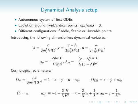
Dynamical Analysis setup

• Autonomous system of first ODEs;

• Evolution around fixed/critical points: dpi/dlna = 0;

• Different configurations: Saddle, Stable or Unstable points

Introducing the following dimensionless dynamical variables:

x =c

3m20H2Ω

, y =c − Λ

3m20H2Ω

, u =ρr

3m20H2Ω

,

αn = −Ω(n+1)

HΩ(n), λm = − (c − Λ)(m+1)

H (c − Λ)(m)

Cosmological parameters:

Ωm =ρm

3m02ΩH2

= 1− x − y − u − α0, ΩDE = x + y + α0,

Ωr = u, weff ≡ −1− 2

3

H

H2= x − 2

3α0 +

1

3α1α0 − y +

1

3u,

Dynamical SystemBackground Eqs & contunuity Eqs → set of first order ODEs, nonlinear,

non-autonomous and hierarchical system

dx

d ln a= λ0y − 6x − 2α0 + xα0 − (α0 + 2x)

H

H2,

dy

d ln a=

(α0 − λ0 − 2

H

H2

)y ,

du

d ln a=

(α0 − 4− 2

H

H2

)u,

dαn−1

d ln a=

(−αn + αn−1 −

H

H2

)αn−1, (n ≥ 1)

dλm−1

d ln a=

(−λm + λm−1 −

H

H2

)λm−1, (m ≥ 1)

whereH

H2= −3

2− 3

2x +

3

2y + α0 −

1

2α1α0 −

1

2u.

Dynamical System

To make the system autonomous we have to impose

αn = const and λm = const

• we fix λ0 = const;

• we allow αn to vary → different couplings.

Working cosmological model:

RDE → MDE→ Accelerated Expansion

Saddle → Saddle → Attractor/Stable Node

Viability: Ωm ≥ 0 , Ωr ≥ 0, weff < − 13

Dynamical Analysis set up

From the definition of the α′s, we see that fixing αN = const gives

Ω(N)(t) = Ω(N)(t0)a−αN ,

Now that we have an expression for the N th derivative of Ω, we can useit to write

Ω(t) =N−1∑i=0

Ω(i)(t0)

i !(t − t0)i + Ω(N)(t0)

∫ t

t0

(t − τ)N−1

(N − 1)!a−αN (τ) dτ,

NOTE: The same for c − Λ!

The Zeroth-order system

• α0 = const and λ0 = const

Ω(t) = Ω0a−α0 , c(t)− Λ(t) = (c − Λ)0a−λ0

P1: matter point → saddle point:α0 = 0 ∧ λ0 < 3

P2: stiff matter point → Unstable node: α0 = 0, weff = 1

P3: DE point → Attractor:(α0 ≥ 3∧α0 +λ0 < 6)∨ (α0 < 1∧λ0 < α0 + 2)∨ (1 ≤ α0 < 3∧λ0 < 3)

P4: radiation point → Saddle point :α0 = 0 ∧ λ0 6= 4

Viable Model: P4 → P1 → P3

α0 = 0→ Ω = const and λ0 < 3allowing for P3 closer to its ΛCDM position λ0 ≈ 0

Reconstructing Quintessence models at zero-th order

EFT functions for Quintessence

c =φ2

2, c − Λ = V (φ) = (c − Λ)0a−λ0

Minimally coupled → α0 = 0

2 1 0 1 2

0.006

0.008

0.01

0.012

0.014

Φm0VΦm

02H

024 2 0 2 4

0.0.5

1.1.5

2.2.5

3.

Log 1z

HH

2

The slow roll parameter and the quintessence potential: α0 = 0, λ0 = 0.1model (blue lines).Planck best fit ΛCDM model (red dashed line) [Ade et al. arXiv:1303.5076

[astro-ph.CO]].

1-st order dynamical system• α1 = const and λ0 = const

Ω(t) = Ω0a−α1 , c(t)− Λ(t) = (c − Λ)0a−λ0

We find 8 critical points:

• Matter point: P1, P5(scaling)• stiff matter point P2

• DE point: P3, P4 (phantom), P6

• Radiation point: P7, P8(scaling)

Viable Transitions:

• Radiation Saddle point: P7

• Matter Saddle point P1

• DE Attractor: P3, P4, P6

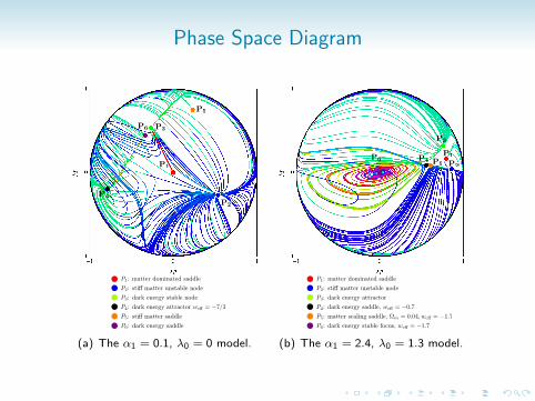
Phase Space Diagram

(a) The α1 = 0.1, λ0 = 0 model. (b) The α1 = 2.4, λ0 = 1.3 model.

Effective equation of state & matter/DE densities

5 4 3 2 1 0 1 2 3 4 50.40.1

0.20.50.81.11.4

Log1z5 4 3 2 1 0 1 2 3 4 5

1.

0.5

0.

0.5

Log1z

wef

f

0.10.20.50.81.1

108642

0

wef

f

0.0.20.40.60.81.

2.52.1.51.0.5

0.

wef

f

Goals

• General tool to investigate Dynamical System of DE/MG models;

• Investigation of general conditions for viability of Ω,Λ, c:• to study perturbations we need to fix the background evolution,• Viable models for Ω → EFTCAMB;

• (Not shown) Study of the recursive nature of the system forλ0 = const :• Families of critical points;• Stability and cosmological viability;• c − Λ grows in time;

• Interesting aspects to work on:• More realizations of the system allowing λm to vary;• Scaling solutions.

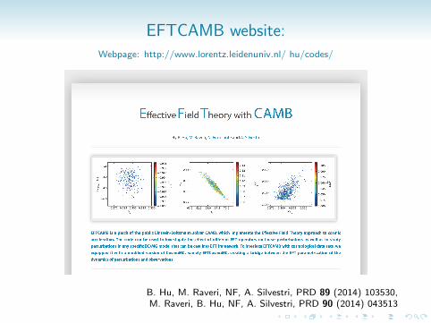
EFTCAMB website:Webpage: http://www.lorentz.leidenuniv.nl/ hu/codes/

B. Hu, M. Raveri, NF, A. Silvestri, PRD 89 (2014) 103530,M. Raveri, B. Hu, NF, A. Silvestri, PRD 90 (2014) 043513

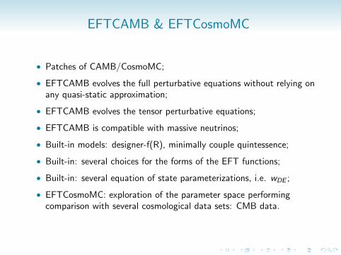
EFTCAMB & EFTCosmoMC

• Patches of CAMB/CosmoMC;

• EFTCAMB evolves the full perturbative equations without relying onany quasi-static approximation;

• EFTCAMB evolves the tensor perturbative equations;

• EFTCAMB is compatible with massive neutrinos;

• Built-in models: designer-f(R), minimally couple quintessence;

• Built-in: several choices for the forms of the EFT functions;

• Built-in: several equation of state parameterizations, i.e. wDE ;

• EFTCosmoMC: exploration of the parameter space performingcomparison with several cosmological data sets: CMB data.

Stability check of perturbations

Deviations from GR are enclosed in the π-field equations:

A(τ, k) π + B(τ, k) π + C (τ)π + k2 D(τ, k)π + E (τ, k) = 0

To ensure that the underlying theory of gravity is stable we place thefollowing theoretical constraints:

• 1 + Ω > 0: the effective Newtonian constant does not change sign;

• A > 0: effective scalar d.o.f. should not be a ghost;

• c2s ≡ D/A ≤ 1: to prevent super-luminary propagation;

• m2π ≡ C/A ≥ 0: to avoid tachyonic instabilities.

EFTCosmoMC: stability requirements become viability priors

EFTCAMB Structure

Standard CAMB

EFTCAMB STRUCTURE(Main EFT flag: EFTflag)

0: GR code

1: pure EFT

Background DE equation of state:(Flag: EFTwDE)

0: LCDM

1: wCDM

2: CPL

3: JBP

4: Turning point

5: Taylor expansion

6: User defined

Pure EFT \Omega model selection:(Flag: PureEFTmodelOmega)

0: Zero

1: Constant

2: Linear model

3: Power law model

4: Exponential model

5: User defined

Pure EFT \alpha_1 model selection:(Flag: PureEFTmodelAlpha1)

Pure EFT \alpha_2 model selection:(Flag: PureEFTmodelAlpha2)

Pure EFT \alpha_3 model selection:(Flag: PureEFTmodelAlpha3)

Pure EFT \alpha_4 model selection:(Flag: PureEFTmodelAlpha4)

Pure EFT \alpha_5 model selection:(Flag: PureEFTmodelAlpha5)

Pure EFT \alpha_6 model selection:(Flag: PureEFTmodelAlpha6)

2: designer matching EFT

Designer EFT model selection:(Flag: DesignerEFTmodel)

1: f(R)

2: minimally coupled quintessence

3: non-minimally coupled quintessence

4: k-essence

5: Horndeski

6: Brans-Dicke

7: …

Background DE equation of state:(Flag: EFTwDE)

0: LCDM

1: wCDM

2: CPL

3: JBP

4: Turning point

5: Taylor expansion

6: User defined

Use someparametrizedforms for the EFT functions

Use a theory whosebackground mimicsexactly the one specified

Notes: B. Hu, M. Raveri, NF, A. Silvestri, arXiv:1405.3590[astro-ph.IM]

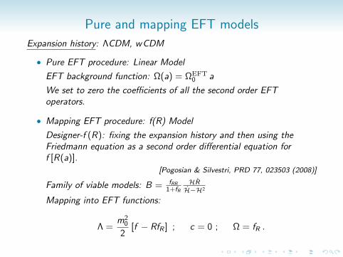
Pure and mapping EFT models

Expansion history: ΛCDM, wCDM

• Pure EFT procedure: Linear Model

EFT background function: Ω(a) = ΩEFT0 a

We set to zero the coefficients of all the second order EFToperators.

• Mapping EFT procedure: f(R) Model

Designer-f (R): fixing the expansion history and then using theFriedmann equation as a second order differential equation forf [R(a)].

[Pogosian & Silvestri, PRD 77, 023503 (2008)]

Family of viable models: B = fRR

1+fR

HRH−H2

Mapping into EFT functions:

Λ =m2

0

2[f − RfR ] ; c = 0 ; Ω = fR .

Results: Stability regions of linear EFT and designer f (R)models

Linear EFT

• viability prior:

ΛCDM: ΩEFT0 ≥ 0

wCDM: ΩEFT0 > 0

ΩEFT0 = 0 → w0 > −1

⇓Quintessence

Designer-f(R)

• viability prior:

ΛCDM: B0 > 0wCDM: w0 not < −1

Results: Bounds for Planck+WP+BAO+Lensing(68% or 95% C.L.)

66

68

70

72

−6.0

−4.5

−3.0

−1.5

0.0

0.250 0.275 0.300 0.325−1.000

−0.992

−0.984

−0.976

−0.968

66 68 70 72 −6.0 −4.5 −3.0 −1.5 0.0

w0

Log 1

0(B

0)H

0Log10 (B0)H0Ωm

b) Designer f(R) on wCDM background

Planck + WP+ BAO+ LensingPlanck + WP+ BAOPlanck + WP55

60

65

70

0.04

0.00

0.08

0.12

0.32 0.40 0.48

−1.0

−0.8

−0.6

55 60 65 70 0.040.00 0.08 0.12

w0

ΩEF

T0

H0

H0Ωm ΩEFT0

a) Linear EFT on wCDM background

Planck + WP+ BAO+ LensingPlanck + WP+ BAOPlanck + WP

ΛCDM: H0 = 68.22± 0.75Ωm = 0.3028± 0.0096ΩEFT

0 < 0.061 (95%C.L.)wCDM:H0 = 67.08± 1.21

Ωm = 0.312± 0.013ΩEFT

0 < 0.058 (95%C.L.)

w0 = −0.95+0.08−0.07 (95%C.L.)

ΛCDM: H0 = 68.41± 0.72Ωm = 0.3005± 0.0092Log10B0 < −2.37 (95%C.L.)

wCDM: H0 = 68.89± 0.75Ωm = 0.2944± 0.0093w0 ∈ (−1,−0.9997) (95%C.L.)Log10B0 = −3.35+1.79

−1.77 (95%)

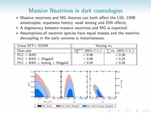
Massive Neutrinos in dark cosmologies• Massive neutrinos and MG theories can both affect the LSS, CMB

anisotropies, expansion history, weak lensing and ISW effects;• A degeneracy between massive neutrinos and MG is expected;• Assumptions:all neutrino species have equal masses and the neutrino

decoupling in the early universe is instantaneous.

Linear EFT+ ΛCDM Varying mν

Data sets ΩEFT0 (95% C.L.)

∑mν (95% C.L.)

PLC + BAO < 0.06 < 0.30PLC + BAO + WiggleZ < 0.06 < 0.25PLC + BAO + lensing + WiggleZ < 0.05 < 0.26

0.00

0.02

0.04

0.06

0.08

0.10

0.15 0.30 0.45 0.60 0.72 0.78 0.84 0.90 0.96 0.72 0.78 0.84 0.90 0.96

0.15

0.30

0.45

0.60

Ω0EF

TΣm

[eV]

ν

Σm [eV]ν σ8 σ8

PLC, BAO PLC, BAO, WiggleZ PLC, BAO, lensing, WiggleZ

Massive Neutrinos in dark cosmologiesf(R)+ΛCDM (95% C.L.) Varying mν Fixing mν

Data sets Log10B0∑

mν Log10B0

PLC + BAO > −6.35 < 0.37 nonePLC + BAO + lensing < −1.0 < 0.43 < −2.3PLC + BAO + lensing + WiggleZ < −3.8 < 0.32 < −4.1PLC + BAO + WiggleZ (EFTCAMB) < −3.8 < 0.30 < −3.9PLC + BAO + WiggleZ (QS f (R)) < −3.2 < 0.24 < −3.7PLC + BAO + WiggleZ (MGCAMB) < −3.1 < 0.23 < −3.5

0.15 0.30 0.45 0.60 -8 -6 -4 -2 0

P / Pm

ax

MGCAMB QS f(R) EFTCAMB

a) PLC, BAO, WiggleZ with massive neutrinos b) without massive neutrinos

Σm [eV]ν

0

-2

-4

-6

-8-8 -6 -4 -2 0

0.0

0.5

1.0

Log

(B

)10

0

Log (B )10 0 Log (B )10 0

• With EFTCAMB less degeneracy due to the exact designerimplementation

Conclusion

EFTCAMB/EFTCosmoMC:

• Evolves full dynamical perturbative equations;

• Evolves the tensor perturbative equations;

• it is compatible with massive neutrinos;

• Allows for model independent test of gravity at large scale;

• Allows to test specific DE/MG models (built-in: f(R); minimallycoupled quintessence);

• built-in stability check.

WHAT’s NEXT?

• Additional DE/MG models of Cosmological interest in the mappingdesigner: BD; Horndeski; Specific galileon models.

• More data set, in particular for LSS test;

• Investigation of the validity of the QS approximation.