Testing cosmological structure formation in Uni ed Dark...
111
UNIVERSIDADE DE LISBOA FACULDADE DE CI ˆ ENCIAS DEPARTAMENTO DE F ´ ISICA Testing cosmological structure formation in Unified Dark Matter-Energy models Diogo Manuel Lopes Castel˜ao Mestrado em F´ ısica especializa¸c˜aoemAstrof´ ısica e Cosmologia Disserta¸c˜ ao orientada por: Ismael Tereno Alberto Rozas-Fern´ andez 2017
Transcript of Testing cosmological structure formation in Uni ed Dark...

UNIVERSIDADE DE LISBOA
FACULDADE DE CIENCIAS
DEPARTAMENTO DE FISICA
Testing cosmological structure formation in UnifiedDark Matter-Energy models
Diogo Manuel Lopes Castelao
Mestrado em Fısicaespecializacao em Astrofısica e Cosmologia
Dissertacao orientada por:Ismael Tereno
Alberto Rozas-Fernandez
2017


i
Agradecimentos
Neste breve pedaco de texto respiro a liberdade de nao escrever exaustivamente sob as normas e formal-idades exigidas adiante. E aproveito-o para agradecer ao doutor Ismael Tereno por ter sido o melhororientador de sempre (e o pior, porque foi o unico) e uma pessoa magnıfica. Ao doutor Alberto Rozas-Fernandez por toda a ajuda, disponibilidade e conversas estimulantes. Agradeco a Katrine, por todaa paciencia e motivacao, por ser bela e estar sempre ao meu lado. Agradeco ao Joao Pereira e aoBartolomeu, por serem o meu refugio emocional. Agradeco a toda a minha famılia, mas agradeco maisao meus pais, a minha irma e ao Ricardo, que me deu abrigo e amizade. Tambem agradeco ao Manuel,a Joana, ao Batalha, ao Joao Gandara, a Joana Filipa, a Sara e a outros amigos por mencionar, porquefazem parte de mim e me inspiram, por vezes expiram, como bons amigos. Dou, por fim, um grandebeijinho ao meu avo, que vive todos os dias no meu pensamento.


iii
Abstract
There is a large number of cosmological models that are able to explain the recent acceleration ofexpansion of the universe. Besides describing the dynamics of the universe, cosmological models alsoneed to correctly predict the observed structure in the universe. The ΛCDM model is in a very goodagreement with most cosmological observations.This thesis deals with an alternative approach, Unified Dark Matter-Energy models (UDM), a classof models that entertains the possibility of a universe where dark matter and dark energy exist as asingle essence. We focus on a model with a fast transition between dark matter-like and dark energy-like behaviours. The rapidity of the transition is an important feature to enable the formation ofstructure. We also discuss another model, the Generalised Chaplygin Gas (GCG), with a small note onthe important effect of non-linear clustering on small scales in this type of models. We implementedthese two models in the Boltzmann Code CLASS which allowed us to obtain the relevant structureformation quantities. From these, we studied the viability of the UDM model using several cosmologicalobservations in an MCMC analysis. The chosen observations were SNe Ia, BAO, CMB and weak lensingdata. At the end of our analysis, we were able to conclude for the first time that this model is able toform structure and is in agreement with structure formation data.
Key words: Unified dark matter-energy models, large scale structure, cosmological parameters, Bayesian in-
ference


v
Resumo em portugues
A dinamica do universo em grandes escalas e dominada pela interacao gravıtica, que actualmente eexplicada pela teoria da Relatividade Geral (GR). Para la da interaccao gravıtica, os componentes quepreenchem o universo e suas interacoes devem ser explicadas pelo modelo padrao da Fısica de partıcu-las. Desta simbiose esperamos poder descrever a evolucao do nosso Universo desde o seu princıpio,comecando na altura em que o universo era um plasma muito quente e denso, com uma taxa de in-teracao entre partıculas elevada. Com a expansao do Universo, a taxa de interacao vai diminuindoe o plasma primordial vai arrefecendo, permitindo a formacao dos primeiros elementos leves como ohidrogenio, helio e lıtio. Quando a densidade de energia diminuiu o suficiente para que os primeiros ato-mos se tornassem estaveis, os fotoes comecaram a propagar-se livremente: este evento e hoje detectadona forma de radiacao de microondas (CMB). Esta radiacao e quase uniforme, com uma temperaturamedia que ronda os 2.7 K em todas as direcoes. No entanto, ele contem pequenas flutuacoes de temper-atura e essas pequenas variacoes representam pequenas nao-homogeneidades na densidade primordialda materia. Essas flutuacoes da materia permitiram a criacao de regioes com uma densidade superiora densidade media e que com o passar do tempo foram crescendo, criando por um lado regioes cadavez mais densas que eventualmente levaram a criacao de galaxias, estrelas e planetas, e por outro ladoregioes de menor densidade que se foram tornando cada vez menos densas, formando grandes zonas de“vazio”. No entanto, a luz do modelo padrao de Fısica de partıculas e da GR nao somos capazes derecriar esta historia do nosso Universo.
Para tornar isso possıvel, em primeiro lugar, logo apos o Big-bang, precisamos introduzir aquilo aque chamamos de inflacao cosmica, um perıodo em que o universo teve uma grande expansao acelerada.Mais tarde, e necessario introduzir dois componentes desconhecidos no Universo. Componentes essesque acabam por ser os elementos mais abundantes do Universo. O primeiro componente desconhecidoe denominado materia escura, e e necessario para a formacao de estrutura. O segundo componente, aenergia escura, e necessario para explicar a actual expansao acelerada do Universo.
A natureza destes dois componentes e actualmente desconhecida e a sua deteccao directa ou indirectae um dos grandes objectivos actuais da cosmologia observacional.
Por parte da cosmologia teorica, a lista de modelos que tenta explicar a actual expansao aceleradado universo, bem como a formacao de estrutura, e extensa. O modelo mais aceite chama-se ΛCDM, emque a energia escura e a constante cosmologica Λ e a materia escura e uma componente fria (CDM).
Nesta dissertacao, exploramos uma alternativa ao modelo ΛCDM, onde se considera que estes doiscomponentes sao na verdade apenas um, havendo uma unificacao da materia escura e da energia escura.Esta abordagem e conhecida como modelos de Unified Dark Matter-Energy (UDM). Em particular,iremo-nos concentrar em descrever e testar com dados observacionais um modelo UDM especıfico quetem uma transicao rapida entre um regime em que se comporta como materia escura e um regime deenergia escura.
Este modelo foi proposto na literatura pelo co-orientador desta dissertacao e colaboradores e naotinha ainda sido testado com dados observacionais de formacao de estrutura. Para fazer uma analise daspropriedades do nosso modelo UDM comecamos no primeiro capıtulo com uma revisao da cosmologiapadrao, onde fazemos referencia ao modelo ΛCDM e dedicamos algum tempo a teoria das perturbacoeslineares. No segundo capıtulo comecamos por fazer um levantamento das varias ideias propostas quantoa origem da energia escura, alternativas ao modelo padrao, e apresentamos uma revisao historica dosmodelos UDM. De seguida, estudamos em detalhe a dinamica do nosso modelo UDM, onde e feitauma analise relativa as perturbacoes e a formacao de estrutura para este modelo. E tambem abordado

vi
o tema das condicoes iniciais para este caso particular, necessarias para resolver numericamente asequacoes de evolucao das perturbacoes. Neste capıtulo e tambem apresentado um outro modelo UDM,o Generalised Chaplygin Gas (GCG), que foi usado como modelo de controlo na implementacao domodelo UDM num codigo de evolucao das perturbacoes lineares. No fim deste capıtulo abordamosainda o efeito de backreaction, isto e, o impacto que as regioes ja colapsadas tem na evolucao dasperturbacoes. Este efeito foi apresentado recentemente na literatura aplicado ao modelo GCG mas etambem aplicavel ao nosso modelo UDM.
O programa usado para o calculo da evolucao das perturbacoes chama-se Cosmic Linear AnisotropySolving System (CLASS) e e apresentado no terceiro capıtulo. Neste capıtulo, apos uma pequenaintroducao sobre o funcionamento do codigo, e feita uma apresentacao detalhada da implementacaode ambos os modelos UDM neste programa. A nossa apresentacao segue a estrutura do CLASS ee dividida em varios modulos (background, perturbations, etc) onde mostramos e analisamos variosresultados obtidos com a implementacao, tais como: a evolucao da densidade de energia, a evolucao daequacao de estado e da velocidade do som, a evolucao da densidade de contraste e o power spectrumda materia.
No capıtulo seguinte, procedemos ao teste do nosso modelo UDM face aos dados observaveis.Comecamos por apresentar os resultados ja publicados do teste a este modelo face a varios observaveisde background, onde o modelo se mostrou tao viavel quanto o modelo ΛCDM.
Tendo em conta que o principal objectivo desta dissertacao e o teste deste modelo na sua capacidadede formar estrutura, fazemos uma pequena revisao teorica do efeito de lentes gravitacionais fracas (weaklensing), uma importante sonda de formacao de estrutura cosmologica.
De seguida sao apresentados os dados usados no teste do nosso modelo: JLA (usando SupernovasIa) e BOSS (usando as oscilacoes acusticas barionicas) como testes de background, Planck (usando oCMB) e KiDS (usando weak lensing) como testes a formacao de estrutura.
Os testes ao modelo, foram feitos com inferencia Bayesiana, usando um codigo Monte Carlo decadeias de Markov, chamado MontePython. Na nossa analise, dividimos o espaco dos parametros emtres regimes e para cada um deles corremos varias cadeias de Markov para diferentes combinacoesde dados e parametros livres. Em particular, fizemos analises com e sem os dados do KiDS, parapermitir isolar a contribuicao das lentes gravitacionais e compreender melhor o seu impacto na analise.Fizemos tambem analises com um maior e menor numero de parametros livres, de modo a diminuir asdegenerescencias entre parametros.
Um aspecto importante a considerar e que com o CLASS calculamos o power spectrum linear damateria, enquanto que a maior parte dos dados medidos pelo KiDS estao no regime nao linear deformacao de estrutura. Depois de apresentada a metodologia adoptada para a analise incluımos oprocedimento usado para lidar com a nao linearidade e apresentamos finalmente os resultados.
Concluımos que o modelo e viavel num dos tres regimes estudados e rejeitado noutro dos regimes.No regime intermedio os resultados sao estatisticamente inconclusivos mas promissores, pois apresentaalgumas das combinacoes de parametros com melhor likelihood no conjunto dos tres regimes.
Em resumo, esta dissertacao mostra pela primeira vez a viabilidade deste modelo na formacaode estrutura, concluindo que e um possıvel candidato para descrever a materia e energia escura, erestringindo os valores dos parametros viaveis em relacao aos encontrados em analise anterior onde omodelo foi testado a nıvel de background.
Identificamos tambem melhoramentos possıveis de efectuar em analises futuras, ao nıvel do trata-mento das integracoes numericas, do tratamento do regime nao-linear e do metodo numerico de amostragem

vii
da distribuicao de probabilidades no espaco dos parametros. E ainda alternativas relacionadas ao mod-elo teorico proposto.
Palavras-chave: Modelos de unificacao de materia e energia escuras, estrutura de grande escala do Universo,
parametros cosmologicos, inferencia Bayesiana

viii

Contents
Agradecimentos i
Abstract iii
Resumo em portugues v
Introduction 9
1 Cosmology 11
1.1 The Homogeneous universe . . . . . . . . . . . . . . . . . . . . . . . . . . . . . . . . . . 11
1.2 Cosmological perturbation theory . . . . . . . . . . . . . . . . . . . . . . . . . . . . . . . 15
1.2.1 Synchronous gauge and Newtonian gauge . . . . . . . . . . . . . . . . . . . . . . 16
1.2.2 Random Fields . . . . . . . . . . . . . . . . . . . . . . . . . . . . . . . . . . . . . 20
2 Unified Dark Matter-Energy models 23
2.1 UDM with fast transition . . . . . . . . . . . . . . . . . . . . . . . . . . . . . . . . . . . 24
2.2 The Generalised Chaplygin Gas . . . . . . . . . . . . . . . . . . . . . . . . . . . . . . . . 30
2.3 Non-linearity (Backreaction) . . . . . . . . . . . . . . . . . . . . . . . . . . . . . . . . . . 31
3 Cosmic Linear Anisotropy Solving System (CLASS) 33
3.1 Input module . . . . . . . . . . . . . . . . . . . . . . . . . . . . . . . . . . . . . . . . . . 35
3.2 Background module . . . . . . . . . . . . . . . . . . . . . . . . . . . . . . . . . . . . . . 37
3.2.1 Results . . . . . . . . . . . . . . . . . . . . . . . . . . . . . . . . . . . . . . . . . 39
3.3 Perturbation module . . . . . . . . . . . . . . . . . . . . . . . . . . . . . . . . . . . . . . 42
3.3.1 Results: evolution of the density contrast . . . . . . . . . . . . . . . . . . . . . . 46
3.4 Other modules . . . . . . . . . . . . . . . . . . . . . . . . . . . . . . . . . . . . . . . . . 50
3.4.1 Results: power spectra . . . . . . . . . . . . . . . . . . . . . . . . . . . . . . . . . 50
4 Testing cosmological models 55
4.1 Background tests . . . . . . . . . . . . . . . . . . . . . . . . . . . . . . . . . . . . . . . . 55
4.2 Tests in the inhomogeneous universe . . . . . . . . . . . . . . . . . . . . . . . . . . . . . 56
4.2.1 Weak gravitational lensing . . . . . . . . . . . . . . . . . . . . . . . . . . . . . . . 56
4.2.2 KiDS Survey . . . . . . . . . . . . . . . . . . . . . . . . . . . . . . . . . . . . . . 60
4.3 Analysis . . . . . . . . . . . . . . . . . . . . . . . . . . . . . . . . . . . . . . . . . . . . . 61
4.3.1 MontePython . . . . . . . . . . . . . . . . . . . . . . . . . . . . . . . . . . . . . . 61
4.3.2 Methodology . . . . . . . . . . . . . . . . . . . . . . . . . . . . . . . . . . . . . . 62

2 CONTENTS
4.3.3 Regime 1: UDM late transition . . . . . . . . . . . . . . . . . . . . . . . . . . . . 654.3.4 Regime 2: UDM mid transition . . . . . . . . . . . . . . . . . . . . . . . . . . . . 684.3.5 Regime 3: UDM early transition . . . . . . . . . . . . . . . . . . . . . . . . . . . 724.3.6 Model comparison . . . . . . . . . . . . . . . . . . . . . . . . . . . . . . . . . . . 75
5 Conclusions 79
Appendices 83
A Results for the GCG 85
B Continuous approximations to the Heaviside function 91
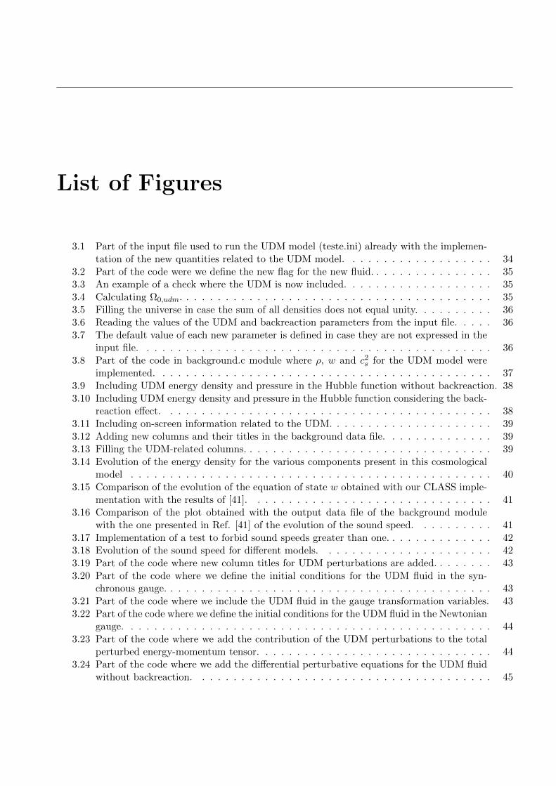
List of Figures
3.1 Part of the input file used to run the UDM model (teste.ini) already with the implemen-tation of the new quantities related to the UDM model. . . . . . . . . . . . . . . . . . . 34
3.2 Part of the code were we define the new flag for the new fluid. . . . . . . . . . . . . . . . 353.3 An example of a check where the UDM is now included. . . . . . . . . . . . . . . . . . . 353.4 Calculating Ω0,udm. . . . . . . . . . . . . . . . . . . . . . . . . . . . . . . . . . . . . . . . 353.5 Filling the universe in case the sum of all densities does not equal unity. . . . . . . . . . 363.6 Reading the values of the UDM and backreaction parameters from the input file. . . . . 363.7 The default value of each new parameter is defined in case they are not expressed in the
input file. . . . . . . . . . . . . . . . . . . . . . . . . . . . . . . . . . . . . . . . . . . . . 363.8 Part of the code in background.c module where ρ, w and c2
s for the UDM model wereimplemented. . . . . . . . . . . . . . . . . . . . . . . . . . . . . . . . . . . . . . . . . . . 37
3.9 Including UDM energy density and pressure in the Hubble function without backreaction. 383.10 Including UDM energy density and pressure in the Hubble function considering the back-
reaction effect. . . . . . . . . . . . . . . . . . . . . . . . . . . . . . . . . . . . . . . . . . 383.11 Including on-screen information related to the UDM. . . . . . . . . . . . . . . . . . . . . 393.12 Adding new columns and their titles in the background data file. . . . . . . . . . . . . . 393.13 Filling the UDM-related columns. . . . . . . . . . . . . . . . . . . . . . . . . . . . . . . . 393.14 Evolution of the energy density for the various components present in this cosmological
model . . . . . . . . . . . . . . . . . . . . . . . . . . . . . . . . . . . . . . . . . . . . . . 403.15 Comparison of the evolution of the equation of state w obtained with our CLASS imple-
mentation with the results of [41]. . . . . . . . . . . . . . . . . . . . . . . . . . . . . . . 413.16 Comparison of the plot obtained with the output data file of the background module
with the one presented in Ref. [41] of the evolution of the sound speed. . . . . . . . . . 413.17 Implementation of a test to forbid sound speeds greater than one. . . . . . . . . . . . . . 423.18 Evolution of the sound speed for different models. . . . . . . . . . . . . . . . . . . . . . 423.19 Part of the code where new column titles for UDM perturbations are added. . . . . . . . 433.20 Part of the code where we define the initial conditions for the UDM fluid in the syn-
chronous gauge. . . . . . . . . . . . . . . . . . . . . . . . . . . . . . . . . . . . . . . . . . 433.21 Part of the code where we include the UDM fluid in the gauge transformation variables. 433.22 Part of the code where we define the initial conditions for the UDM fluid in the Newtonian
gauge. . . . . . . . . . . . . . . . . . . . . . . . . . . . . . . . . . . . . . . . . . . . . . . 443.23 Part of the code where we add the contribution of the UDM perturbations to the total
perturbed energy-momentum tensor. . . . . . . . . . . . . . . . . . . . . . . . . . . . . . 443.24 Part of the code where we add the differential perturbative equations for the UDM fluid
without backreaction. . . . . . . . . . . . . . . . . . . . . . . . . . . . . . . . . . . . . . 45

4 LIST OF FIGURES
3.25 Part of the code where we add the differential perturbative equations for the UDM fluidwith backreaction. . . . . . . . . . . . . . . . . . . . . . . . . . . . . . . . . . . . . . . . 45
3.26 Part of the code where we add the contribution of the UDM perturbations to the δm. . 46
3.27 Evolution of the density contrast for several UDM models for a large scale. . . . . . . . 47
3.28 Evolution of the density contrast for several UDM models for a intermediate scale. . . . 47
3.29 Evolution of the density contrast for several UDM models for a small scale. . . . . . . . 48
3.30 Evolution of the density contrast for a GCG model a large scale. . . . . . . . . . . . . . 49
3.31 Temperature angular power spectrum of the CMB for different values of the model pa-rameters. . . . . . . . . . . . . . . . . . . . . . . . . . . . . . . . . . . . . . . . . . . . . 50
3.32 Matter power spectrum for different values of model parameters (first part). . . . . . . . 52
3.33 Matter power spectrum for different values of model parameters (second part). . . . . . 53
4.1 Ilustration of the lens effect. . . . . . . . . . . . . . . . . . . . . . . . . . . . . . . . . . . 57
4.2 Example of Input file used to run MontePython. . . . . . . . . . . . . . . . . . . . . . . 62
4.3 Regime 1: Posterior probabilities for each parameter in the minimal set-up, as well asthe contours with the 1-σ and 2-σ confidence regions. . . . . . . . . . . . . . . . . . . . 66
4.4 Regime 1: Posterior probabilities for each parameter in the vanilla set-up, as well as thecontours with the 1-σ and 2-σ confidence regions. . . . . . . . . . . . . . . . . . . . . . . 68
4.5 Regime 2: Posterior probabilities for each parameter in the minimal set-up, as well asthe contours with the 1-σ and 2-σ confidence regions. . . . . . . . . . . . . . . . . . . . 70
4.6 Regime 2: Posterior probabilities for each parameter in the vanilla set-up, as well as thecontours with the 1-σ and 2-σ confidence regions. . . . . . . . . . . . . . . . . . . . . . . 71
4.7 Regime 3: Posterior probabilities for each parameter in the minimal set-up, as well asthe contours with the 1-σ and 2-σ confidence regions. . . . . . . . . . . . . . . . . . . . 73
4.8 Regime 3: Posterior probabilities for each parameter in the vanilla set-up, as well as thecontours with the 1-σ and 2-σ confidence regions. . . . . . . . . . . . . . . . . . . . . . . 75
A.1 Evolution of the density contrast for a GCG model for a intermediate scale. . . . . . . . 86
A.2 Evolution of the density contrast for a GCG model for a small scale. . . . . . . . . . . . 86
A.3 Matter power spectrum for a GCG model. . . . . . . . . . . . . . . . . . . . . . . . . . . 87
A.4 Evolution of the density contrast for a GCG model with backreaction for a large scale. . 87
A.5 Evolution of the density contrast for a GCG model with backreaction for a intermediatescale. . . . . . . . . . . . . . . . . . . . . . . . . . . . . . . . . . . . . . . . . . . . . . . . 88
A.6 Evolution of the density contrast for a GCG model with backreaction for a small scale. . 89
A.7 Matter power spectrum for a GCG model with backreaction. . . . . . . . . . . . . . . . 89
B.1 Sound speed for the first attempt of a continuous approximation to the Heaviside stepfunction. . . . . . . . . . . . . . . . . . . . . . . . . . . . . . . . . . . . . . . . . . . . . . 92
B.2 Matter power spectrum for the first attempt of a continuous approximation to the Heav-iside step function. . . . . . . . . . . . . . . . . . . . . . . . . . . . . . . . . . . . . . . . 92
B.3 Sound speed for the second attempt of a continuous approximation to the Heaviside stepfunction. . . . . . . . . . . . . . . . . . . . . . . . . . . . . . . . . . . . . . . . . . . . . . 93
B.4 Sound speed for the fourth attempt of a continuous approximation to the Heaviside stepfunction. . . . . . . . . . . . . . . . . . . . . . . . . . . . . . . . . . . . . . . . . . . . . . 94
B.5 Matter power spectrum for the fourth attempt of a continuous approximation to theHeaviside step function (first case) . . . . . . . . . . . . . . . . . . . . . . . . . . . . . . 95

LIST OF FIGURES 5
B.6 Matter power spectrum for the fourth attempt of a continuous approximation to theHeaviside step function (second case) . . . . . . . . . . . . . . . . . . . . . . . . . . . . . 95

6 LIST OF FIGURES

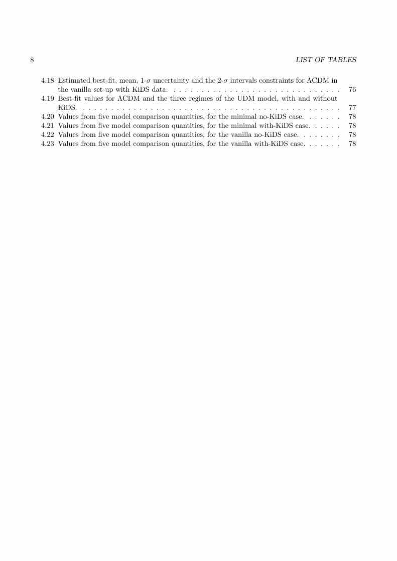
List of Tables
4.1 Summary of the constraints (median values and 1-σ intervals) for the model parametersusing CMB, BAO and SN data. The minimum reduced χ2 and the Bayes factor withrespect to ΛCDM are also shown. . . . . . . . . . . . . . . . . . . . . . . . . . . . . . . . 56
4.2 The allowed ranges for the parameters of the model in the three cases. . . . . . . . . . . 64
4.3 Estimated best-fit, mean, 1-σ uncertainty and 2-σ intervals constraints for regime 1 inthe minimal set-up without KiDS data. . . . . . . . . . . . . . . . . . . . . . . . . . . . 65
4.4 Estimated best-fit, mean, 1-σ uncertainty and the 2-σ intervals constraints for regime 1in the minimal set-up with KiDS data. . . . . . . . . . . . . . . . . . . . . . . . . . . . . 66
4.5 Estimated best-fit, mean, 1-σ uncertainty and the 2-σ intervals constraints for regime 1in the vanilla set-up without KiDS data. . . . . . . . . . . . . . . . . . . . . . . . . . . . 67
4.6 Estimated best-fit, mean, 1-σ uncertainty and the 2-σ intervals constraints for regime 1in the vanilla set-up with KiDS data. . . . . . . . . . . . . . . . . . . . . . . . . . . . . . 67
4.7 Estimated best-fit, mean, 1-σ uncertainty and the 2-σ intervals constraints for regime 2in the minimal set-up without KiDS data. . . . . . . . . . . . . . . . . . . . . . . . . . . 69
4.8 Estimated best-fit, mean, 1-σ uncertainty and the 2-σ intervals constraints for regime 2in the minimal set-up with KiDS data. . . . . . . . . . . . . . . . . . . . . . . . . . . . . 69
4.9 Estimated best-fit, mean, 1-σ uncertainty and the 2-σ intervals constraints for regime 2in the vanilla set-up without KiDS data. . . . . . . . . . . . . . . . . . . . . . . . . . . . 70
4.10 Estimated best-fit, mean, 1-σ uncertainty and the 2-σ intervals constraints for regime 2in the vanilla set-up with KiDS data. . . . . . . . . . . . . . . . . . . . . . . . . . . . . . 71
4.11 Estimated best-fit, mean, 1-σ uncertainty and the 2-σ intervals constraints for regime 3in the minimal set-up without KiDS data. . . . . . . . . . . . . . . . . . . . . . . . . . . 72
4.12 Estimated best-fit, mean, 1-σ uncertainty and the 2-σ intervals constraints for regime 3in the minimal set-up with KiDS data. . . . . . . . . . . . . . . . . . . . . . . . . . . . . 73
4.13 Estimated best-fit, mean, 1-σ uncertainty and the 2-σ intervals constraints for regime 3in the vanilla set-up without KiDS data. . . . . . . . . . . . . . . . . . . . . . . . . . . . 74
4.14 Estimated best-fit, mean, 1-σ uncertainty and the 2-σ intervals constraints for regime 3in the vanilla set-up with KiDS data. . . . . . . . . . . . . . . . . . . . . . . . . . . . . . 74
4.15 Estimated best-fit, mean, 1-σ uncertainty and the 2-σ intervals constraints for ΛCDM inthe minimal set-up without KiDS data. . . . . . . . . . . . . . . . . . . . . . . . . . . . 75
4.16 Estimated best-fit, mean, 1-σ uncertainty and the 2-σ intervals constraints for ΛCDM inthe minimal set-up with KiDS data. . . . . . . . . . . . . . . . . . . . . . . . . . . . . . 76
4.17 Estimated best-fit, mean, 1-σ uncertainty and the 2-σ intervals constraints for ΛCDM inthe vanilla set-up without KiDS data. . . . . . . . . . . . . . . . . . . . . . . . . . . . . 76
8 LIST OF TABLES
4.18 Estimated best-fit, mean, 1-σ uncertainty and the 2-σ intervals constraints for ΛCDM inthe vanilla set-up with KiDS data. . . . . . . . . . . . . . . . . . . . . . . . . . . . . . . 76
4.19 Best-fit values for ΛCDM and the three regimes of the UDM model, with and withoutKiDS. . . . . . . . . . . . . . . . . . . . . . . . . . . . . . . . . . . . . . . . . . . . . . . 77
4.20 Values from five model comparison quantities, for the minimal no-KiDS case. . . . . . . 784.21 Values from five model comparison quantities, for the minimal with-KiDS case. . . . . . 784.22 Values from five model comparison quantities, for the vanilla no-KiDS case. . . . . . . . 784.23 Values from five model comparison quantities, for the vanilla with-KiDS case. . . . . . . 78

Introduction
The dynamics of the universe on large scales is dominated by the gravitational interaction, which is, inthe standard view, explained by the theory of General Relativity (GR). On the other hand, the contentsof the universe and their interactions besides gravity are expected to be explained by the standard modelof particle physics. From this symbiosis we expect to be able to describe our universe from the verybeginning, when the universe was a very hot and dense plasma, matter was in the form of free electronsand atomic nuclei and the interactions between particles were very energetic and frequent, to the veryend. In the thermal evolution of the universe, the primordial plasma cooled down and light elementslike hydrogen, helium and lithium were formed. When the energy dropped enough for the first stableatoms to exist, the universe transparent and the photons have been propagating freely since, and wenow observe them in the form of microwave radiation (CMB). This radiation is almost uniform, withthe same temperature of about 2.7 K in all directions. However, this CMB contains small fluctuationsin temperature and those tiny variations represent small inhomogeneities in the primordial density ofmatter. As time passed by, this matter fluctuation grew and overdense regions became increasinglydenser leading to the creation of galaxies, stars and planets. This brief history is well known, andnowadays it seems to be so right that even when we were small children that history made perfectsense. What causes a child, that has no deep knowledge of physics, to feel this idea to be true goesbeyond this dissertation, but the most important thing is that we are, unfortunately, not able to recreatethe universe dynamics if we rely only on the standard model of particle physics and on standard GR.
First of all, we need to introduce inflation at the the very beginning. Later on, some exotic com-ponents must also be introduced that turn out to dominate the matter-energy content of the universe.These are dark matter (DM), needed to form structure, and dark energy (DE), required to explain thelate-time accelerated expansion of the universe. The true nature of these two components is unknownand the search for it is an ongoing quest of cosmological studies. The first step in this quest is to assessif a certain model of DM and DE matches our current observations. There are many models proposedthat pass this first test. However, these several ideas have different characteristics, even if they try toreplicate the same universe. This pushes the searches for the nature of these components to increasinglevels of precision, where we try to find small signatures that distinguish a model from another.
In this dissertation we explore the elegant idea of considering that the two components are in factjust one. This approach is known as the Unified Dark Matter-Energy models (UDM). More specifically,we focus on describing and testing a specific UDM model that has a fast transition from a DM likebehavior to a DE like one. In order to fully describe the properties of our UDM model of interestwe start, in chapter 1, with a review of standard cosmology, with an emphasis on linear perturbationtheory, and proceed in chapter 2 with the detailed description of the model. We also introduce inchapter 2 another type of unified model, the well-known Generalised Chaplygin Gas (GCG) (includingback-reaction effects), that we will use as a benchmark in implementation tests. In order to test the

10 LIST OF TABLES
model, we start by implementing it in the Cosmic Linear Anisotropy Solving System (CLASS). CLASSis a software program designed to compute the evolution of linear perturbations in the universe. Thedetails of the modifications of CLASS for both models are presented in chapter 3, where we also furtherdiscuss the properties of the models now supported by outputs of CLASS, such as the matter powerspectrum. We then move to the actual model testing in chapter 4. Here we perform several Bayesianinference analyses using the Markov Chain Monte Carlo (MCMC) code MontePython. The UDM modelwith fast transition is tested against various sets of cosmological structure formation and backgroundexpansion data (JLA Supernova data, BOSS BAO data, Planck CMB data and KiDS weak lensingdata) using various sets of varying and fixed cosmological and nuisance parameters. We conclude inchapter 5, showing for the first time the viability of this model at structure formation level, implyingthat the UDM approach is still a possible candidate to describe DM and DE.

Chapter 1
Cosmology
1.1 The Homogeneous universe
Standard Big Bang cosmology rests on two fundamental assumptions:
-When we average over a sufficiently large scale, the observable properties of the universe areisotropic. In particular, the microwave background is almost perfectly isotropic and the distributionof distant galaxies approaches isotropy, while on the contrary nearby galaxies are very anisotropicallydistributed.
-Our position in the universe is by no means preferred to any other. This implies that the firstassumption must hold for every observer in the universe. But if the universe is isotropic around all itspoints, it is also necessarily homogeneous.
These two assumptions requiring that the universe is homogeneous and isotropic when averagingover larges volumes are expressed, in general relativity, on the Friedmann-Lemaitre-Robertson-Walker(FLRW) metric:
ds2 = gµνdxµdxν = −dt2 + a2
[dr2
1− kr2 + r2(dθ2 + sin(θ)2dϕ2)], (1.1)
usually written as
ds2 = dt2 − a2(t)γijdxidxj , (1.2)
where a(t) is known as the scale factor, t is the cosmic time and k is the space curvature. For k > 0 theuniverse is closed. For k = 0 the universe is flat. For k < 0 the universe is open, having a hyperbolicspatial section.
In addition to the cosmic time t, it is also convenient to introduce the conformal time defined by
τ ≡∫a−1dt. (1.3)
The Einstein equations, describing the dynamics of the universe, can be computed as follows [1, 2].From the metric gµν , we first obtain the Christoffel symbols

12 CHAPTER 1. COSMOLOGY
Γµνδ = 12g
µα(gαν,δ + gαδ,ν − gνδ,α) , (1.4)
with gαν,δ = ∂gαν∂xδ
. The Ricci curvature tensor is then defined by
Rµν = Γαµν,α − Γαµα,ν + ΓαµνΓβαβ − ΓαµβΓβαν , (1.5)
and can contracted in order to get the Ricci scalar
R = gµνRµν . (1.6)
The desired Einstein field equations can be obtained from the following action
S =∫d4x√−g
[R
16πG + LM
], (1.7)
where the first term in the action comes from the Einstein-Hilbert action and the LM represents all thematter fields present.
From the principle of least action we have
0 = δS =∫d4x
[ 116πG
δ (√−gR)
δgµν+ δ (
√−gLM )δgµν
]δgµν
=∫d4x√−g
[ 116πG
(δR
gµν+ R√−g
δ√−g
δgµν
)+ 1√−g
δ (√−gLM )δgµν
]δgµν . (1.8)
Since this should hold for any variation with respect to gµν , it follows that
δR
gµν+ R√−g
δ√−g
δgµν= 8πG (−2)√
−gδ (√−gLM )δgµν
. (1.9)
The right-hand side of the equation is the energy-momentum tensor
Tµν = − 2√−g
δ (√−gLM )δgµν
, (1.10)
that contains the density and pressure of all the cosmological fluids (the source of gravity). By definingthe properties of each fluid we determine the cosmic expansion.
It was proved in [4] that the variation of the Ricci scalar R and the variation of the determinant gis
δR
δgµν= Rµν (1.11)
δg = δdet(gµν) = ggµνδgµν ⇒1√−g
δ√−g
δgµν= −1
2gµν , (1.12)
which allow us to rewrite the right-hand side of Eq.(1.9) and obtain the Einstein equations
Rµν −12gµνR = Gµν = 8πGTµν , (1.13)

1.1. THE HOMOGENEOUS UNIVERSE 13
where Gµν is the Einstein tensor.The dynamical evolution of the universe is known once we solve the Einstein equations of General
Relativity [1, 2, 5].For the FLRW metric Eq.(1.2), the non-vanishing Christoffel symbols are
Γ0ij = aaγij , (1.14)
Γi0j = a
aδij , (1.15)
Γijk = 12γ
ij (∂jγkl + ∂kγjl − ∂lγjk) . (1.16)
From that we get the following non-vanishing components of the Ricci tensor and the Ricci scalar
R00 = −3 aa, (1.17)
Rij = −[a
a+ 2
(a
a
)2+ 2 k
a2
]gij , (1.18)
R = −6[a
a+(a
a
)2+ k
a2
], (1.19)
and we obtain the non-vanishing components of the Einstein tensor
G00 = 3
[(a
a
)2+ k
a2
], (1.20)
Gij =[2 aa
+(a
a
)2+ k
a2
]δij , (1.21)
with Gµν = gµδGδν . Here a dot represents the derivative with respect to the cosmic time t.The Einstein equations can be reduced to two differential equations by combining Eqs. (1.20) and
(1.21) with the energy-momentum tensor Eq.(1.10)(a
a
)2= 8πG
3 ρ− K
a2 + Λ3 , (1.22)
a
a= −4πG
3 (ρ+ 3p) + Λ3 . (1.23)
Eqs.(1.22) and (1.23), the Friedmann equations, can be combined to give the continuity equation
d
dt(a3ρ) + p
d
dt(a3) = 0 , (1.24)
which intuitively states energy conservation: the first term is the change in internal energy and thesecond term is the pressure work. This is the first law of thermodynamics in the absence of heat flow(which would violate isotropy).

14 CHAPTER 1. COSMOLOGY
The universe is filled with different matter components (barotropic fluids) that will provide the lastequation needed to solve the set of equations, the equation of state
w = p
ρ, (1.25)
which relates the energy density and pressure of the various possible cosmological fluids. For cold darkmatter (CDM) (w = 0), radiation (w = 1/3), vacuum energy (w = −1) or for any other barotropic fluidwith a dynamical equation of state w(a), the solution to Eq.(1.24) is
ρ(a) = ρ(a0)e−∫ aa0
3(1+w(a))a−1da. (1.26)
ΛCDM model
The simplest model capable of explaining several evidences observed in our real universe is ΛCDM. It isa universe filled with two main components of unknown nature: the cosmological constant Λ, responsiblefor the late accelerated expansion of the universe, and CDM, as the main component driving structureformation and of structure itself. In the ΛCDM model Eq.(1.22) becomes(
a
a
)2= H2 = 8πG
3
[ρr
(a0a
)4+ ρm
(a0a
)3+ ρΛ
], (1.27)
where ρi denotes the energy density of the different components of the energy budget today, at t = t0.We will also use the conventional normalisation for the scale factor, a0 ≡ 1.
For a flat universe, the critical density today is [2, 5]
ρcrit = 3H20
8πG = 1.1× 10⁻⁵h2 protonscm3 , (1.28)
and we use the critical density to define the dimensionless density parameter
Ωi = ρiρcrit
. (1.29)
Then the Friedmann equation (1.27) becomes
H2(a) = E2H20 = H2
0
[Ωr
(a0a
)4+ Ωm
(a0a
)3+ ΩΛ
]. (1.30)
A combination of several cosmological observations have allowed the Planck team to estimate thedensity parameters of the ΛCDM model with high precision [6]. Their central values are Ωr = 9.4×10⁻⁵,Ωm = 0.31 and ΩΛ = 0.68. The matter density parameter, Ωm, has contributions around 0.04 of ordi-nary (baryonic) matter and 0.27 of DM. [2, 5].

1.2. COSMOLOGICAL PERTURBATION THEORY 15
1.2 Cosmological perturbation theory
So far, we considered the universe as perfectly homogeneous. To understand the formation and evolutionof large-scale structures, we have to introduce inhomogeneities. As long as these perturbations remainrelatively small, we can define a metric that deviates from the FLRW spacetime as the sum of theunperturbed FLRW part plus something else, that is usually called the perturbed metric.
gµν = g(0)µν + δgµν . (1.31)
Then, by using the flat FLRW background spacetime with no curvature,
ds2 = a2(τ)[−dτ2 + δijdx
idxj], (1.32)
the perturbed metric is
ds2 = a2(τ)[−(1− 2A)dτ2 + 2Bidxidτ − (δij + hij)dxidxj
]. (1.33)
where A, Bi and hij are functions of space and time.Now that we have defined the perturbed metric it is important to perform a scalar-vector-tensor
(SVT) decomposition of the perturbations, that will allow us to get the Einstein equations for scalars,vectors and tensors unmixed at linear order and will allow us to treat them separately [2].
For the 3-vector Bi we can split it into the gradient of a scalar plus a divergenceless vector
Bi = ∂iB + Bi, (1.34)
with ∂iBi = 0.The rank-2 simmetric tensor can be written as
hij = 2Cδij + 2(∂i∂j −
13δij∇
2)E +
(∂iEj + ∂jEi
)+ 2Eij , (1.35)
where the tensor perturbation is traceless, Eii = 0, ∂iEi and ∂iEij = 0.This allow us to re-writte the 10 degrees of freedom of the metric as 4 scalar, 4 vectors and 2 tensors
components.
Here we have to take into account a small consideration. The metric perturbations that we definedEq.(1.33) were made by choosing a specific time slicing of the spacetime and a defined specific spatialcoordinates on this time slice. Then, by making a different choice of coordinates we can change thevalues of these perturbations variables and we can introduce fake perturbations or even remove trueones. For example, if we take the homogeneous FLRW metric Eq.(1.32) and make the following changeof the spatial coordinates xi → xi = xi+εi(τ, ~x), where we assume εi to be small and therefore amenableto being treated as a perturbation. With dxi = dxi − ∂τ εidτ − ∂kεidxk, the FLRW metric Eq.(1.32)becomes
ds2 = a2(τ)[−dτ2 + 2∂τ εidxidτ − (δij + ∂iεj + ∂jεi) dxidxj
], (1.36)
dropping the quadratic terms in εi. We have apparently introduced the metric perturbations Bi = ∂τ εiand Ei = εi, but these are just fictitious gauge modes that can be removed by going back to the oldcoordinates. In the same way, we can change our time slicing, τ → τ + ε0(τ, ~x), and the homogeneous

16 CHAPTER 1. COSMOLOGY
energy density of the universe gets perturbed, ρ(τ)→ ρ(τ + ε0(τ, ~x)) = ρ(τ) + ρ′ε0. This means that a
change of the time coordinate can lead to fake density perturbations, δρ = ρ′ε0. On the other hand, a
real perturbation in the perturbed metric can be removed in the same way by a change of coordinates.These examples show us that we need a more physical way to identify true perturbations. One
way to avoid the gauge problems is to define a special combination of metric perturbations that do nottransform under a change of coordinates. These are called Bardeen variables. Another alternative is tofix the gauge and keep track of all perturbations.
1.2.1 Synchronous gauge and Newtonian gauge
Throughout this dissertation we will consider two gauges, the synchronous gauge and the Newtoniangauge, because they are the ones that will be used later in CLASS. Also, thanks to the SVT decompo-sition, we are able to only consider the scalar perturbations, since vector and tensor perturbations arenot of much interest in current DE research. In this case, Eq.(1.33) becomes,
ds2 = a2(τ)[− (1 + 2A) dτ2 + 2∂iBdτdxi + [(1 + 2C)δij + 2∂i∂jE] dxidxj
]. (1.37)
The synchronous gauge is the most commonly used gauge, adopted by Lifshitz [3]. For this gaugethe components g00 and g0i of the metric tensor are by definition unperturbed, i.e., A = B = 0, andthe line element is usually written as
ds2 = a2(τ)[−dτ2 + [(1 + 2C)δij + 2∂i∂jE] dxidxj
]. (1.38)
These two scalar fields (C and E) characterise the scalar mode of hij . The scalar mode of hij is
usually written as a Fourier integral, as a function of two fields h(~k, τ) and η(~k, τ):
hij(~x, τ) =∫d3kei
~k~x[kikjh(~k, τ) + (kikj −
13δij)6η(~k, τ)
](1.39)
In addition, to fix the gauge we need to impose the extra condition that the synchronous gauge iscomoving with pressureless species i.
For the Newtonian gauge we fix two of the scalar perturbations to zero E = B = 0, which gives themetric:
ds2 = a2(τ)[− (1 + 2Ψ) dτ2 + (1− 2Φ)δijdxidxj
], (1.40)
where we renamed A ≡ Ψ and C ≡ −Φ, as it is usually defined in the literature.
With all this set we will now derive the first order Einstein equations using the Newtonian gauge.To do that we decompose the Einstein tensor Gµν and the energy-momentum tensor Tµν into a
background part and a perturbed part
Gµν = Gµ(0)ν + δGµν (1.41)
Tµν = Tµ(0)ν + δTµν . (1.42)
The background part was already solved in the previous section. The perturbed part of the Einsteinequation is then given by

1.2. COSMOLOGICAL PERTURBATION THEORY 17
δGµν = 8πGδTµν . (1.43)
First we need to calculate the perturbed Christoffel symbols
δΓµνλ = 12δg
µα (gαν,λ + gαδ,ν − gνλ,α) + 12g
µα (δgαν,λ + δgαδ,ν − δgνλ,α) . (1.44)
For the the metric Eq.(1.40), the non-zero components are
δΓ0ij = δij
[2H (Φ−Ψ) + Φ′
], (1.45)
δΓ000 = Ψ′, (1.46)
δΓ00i = δΓi00 = Ψ,i, (1.47)
δΓij0 = δijΦ′. (1.48)
Here a prime represents the derivative with respect to the conformal time τ . Next, we derive theperturbation in the Ricci tensor and scalar
δRµν = δΓαµν,α − δΓαµα,ν + δΓαµνΓβαβ + ΓαµνδΓβαβ − δΓ
αµβΓβαν − ΓαµβδΓβαν (1.49)
δR = δgµαRαµ + gµαδRαµ, (1.50)
with this we obtain the perturbed Einstein tensor
δGµν = δRµν −12δgµνR−
12gµνδR (1.51)
δGµν = δgµαGαν + gµαδGαν . (1.52)
Inserting all these quantities, we can write the perturbed Einstein tensor as function of the metriccomponents [1]
δG00 = 2a−2
[3H
(HΨ− Φ′
)+∇2Φ
], (1.53)
δG0i = 2a−2∇i
(Φ′ −HΨ
), (1.54)
δGij = 2a−2[(H2 + 2H′
)Ψ +HΨ′ − Φ′′ − 2HΦ′
]δij + a−2
[∇2 (Ψ + Φ) δij −∇ij (Ψ + Φ)
]. (1.55)
Notice that we defined the conformal Hubble function H ≡ Ha.Now we will take a look at the perturbed energy momentum tensor Tµν , where we will consider it
to be the energy momentum tensor of a single perfect fluid. As we will see later, this is what we needto implement a UDM model in CLASS.

18 CHAPTER 1. COSMOLOGY
For a perfect fluid, the energy momentum tensor is
Tµν = Tµ(0)ν + δTµν , (1.56)
where the unperturbed part is given by
Tµ(0)ν = (ρ+ P ) uµuν + Pδµν . (1.57)
The perturbed part is then
δTµν = (δρ+ δP )uµuν + (ρ+ P )(uµδuν + uνδuµ) + δPδµν , (1.58)
that we can rewrite as
δTµν = ρ[δ(1 + c2
s)uν uµ + (1 + w)(δuν uµ + uνδuµ) + c2
sδδµν
]. (1.59)
Here we introduced important quantities, the density contrast and the sound speed
δ ≡ δρ
ρ, (1.60)
c2s ≡
δP
δρ. (1.61)
If the fluid is barotropic, P = P (ρ), then c2s = P ′/ρ′.
We also have to define the 4-velocity vector uµ = a−1δ0µ. Since gµνu
µuν = 1 and gµν uµuν = 1, we
have at linear order
δgµν uµuν + 2uµδuµ = 0. (1.62)
For the Newtonian gauge δg00 = 2a2Ψ, we get δu0 = −Ψa−1, and we write the spatial part of theperturbed 4-velocity vector as δui ≡ vi/a, with vi ≡ dxi/dτ . So we have
uµ = a−1[(1−Ψ) , vi
], (1.63)
uµ = gµνuν = [−a (1 + Ψ) , avi] . (1.64)
The perturbed components of the energy-momentum tensor are then
δT 00 = −δρ (1.65)
δT 0i = −δT i0 = (1 + w)ρvi (1.66)
δT 11 = δT 2
2 = δT 33 = c2
sδρ. (1.67)
We finally obtain the perturbed Einstein equations
3H(HΨ− Φ′
)+∇2Φ = 4πGa2δT 0
0 = −4πGa2ρδ, (1.68)

1.2. COSMOLOGICAL PERTURBATION THEORY 19
∇2 (Φ′ −HΨ)
= 4πGa2(ρ+ P )θ = 4πGa2(1 + w)ρθ, (1.69)
Ψ = −Φ, (1.70)
Φ′′ + 2HΦ′ −HΨ′ −(H2 + 2H′
)Ψ = −4πGa2c2
sρδ, (1.71)
where we introduced the velocity divergence θ ≡ ∇ivi, where in the synchronous gauge θi = 0 for anypressureless species.
The energy-momentum tensor satisfies the identity ∇µTµν = 0. And for the perturbed part it writes
∇µδTµν = δTµν,µ − δΓανβT βα − ΓανβδT βα + δΓαβαT βν + ΓαβαδT βν = 0. (1.72)
For the component ν = 0, we obtain a continuity equation
∂τ (δρ) + 3H (δρ+ δP ) = − (ρ+ P )(θ + 3Φ′
), (1.73)
and using the unperturbed continuity equation (1.24) we get
δ′ + 3H(c2s − w
)δ = − (1 + w)
(θ + 3Φ′
). (1.74)
The equation ∇µδTµν = 0 for ν = i leads to
θ′ +[H(1− 3w) + w′
1 + w
]θ = −∇2
(c2s
1 + wδ + Ψ
). (1.75)
We can rewrite the perturbed Einstein equations (1.68)-(1.71) and the conservation equations (1.74),(1.75) in Fourier space, yielding
3H(HΨ− Φ′
)+ k2Φ = 4πGa2δT 0
0 = −4πGa2ρδ, (1.76)
k2 (Φ′ −HΨ)
= 4πGa2(ρ+ P )θ = 4πGa2(1 + w)ρθ, (1.77)
Ψ = −Φ, (1.78)
Φ′′ + 2HΦ′ −HΨ′ −(H2 + 2H′
)Ψ = −4πGa2c2
sρδ, (1.79)
δ′ + 3H(c2s − w
)δ = − (1 + w)
(θ + 3Φ′
), (1.80)
θ′ +[H(1− 3w) + w′
1 + w
]θ = −k2
(c2s
1 + wδ + Ψ
). (1.81)
Following the same procedure for the synchronous gauge we arrive at an equivalent set of equations[7]

20 CHAPTER 1. COSMOLOGY
k2η − 12Hh
′ = 4πGa2δT 00 = −4πGa2ρδ, (1.82)
k2η′ = 4πGa2(ρ+ P )θ = 4πGa2(1 + w)ρθ, (1.83)
h′′ + 2Hh′ − 2k2η = −8πGa2δT ii = −24πGa2c2sρδ, (1.84)
h′′ + 6η′′ + 2H(h′ + 6η′)− 2k2η = −24πG(ρ+ P )σ, (1.85)
δ′ + 3H(c2s − w
)δ = − (1 + w)
(θ + h′
2
), (1.86)
θ′ +[H(1− 3w) + w′
1 + w
]θ = k2 c2
s
1 + wδ. (1.87)
The conservation equations both in the synchronous and in the Newtonian gauge are valid for asingle uncoupled fluid, or for the total δ and θ that include all fluids.
1.2.2 Random Fields
It is important to note that all perturbed quantities are random fields and not deterministic quantities.Indeed, the structures that we see today arrive from the quantum fluctuations of the energy densityfrom the very beginning of the universe. At that time, the energy density at each point results from astochastic process. As such, initial conditions for δ as a function of spatial location cannot be known,but only its statistical distribution. The primordial distributions are assumed to be Gaussian and aredescribed by the mean, which is 〈δ〉 = 0 by definition, and the variance. The variance defines a matrixin real space (the covariance matrix, a 2-point quantity in the space of spatial coordinates) and it is thecentral quantity to describe structure formation in cosmology. This implies that, due to the randomnessof initial conditions, the goal of structure formation studies is not to determine the values of δ at givenlocations, but to determine the covariance matrix of the δ field.
As an example let us start by considering N galaxies in a volume V (assuming that galaxies tracethe δ field). We can calculate the average numerical density as ρ0 = N/V , but this will not tell us if theN points are evenly distributed across the volume or if they are distributed inhomogeneously. Indeed,that information is contained in the covariance matrix. What we can do is then analyse a smallervolume dV inside the volume V , where ρ0dV is still the average number of points in this infinitesimalvolume. Let us define dNab = 〈nanb〉 as the product of the number of points in one volume times thenumber of points in the other volume, separated by rab
dNab = 〈nanb〉 = ρ20dVadVb [1 + ξ(rab)] . (1.88)
The excess number of pairs in the volumes dVa and dVb, compared with the number of pairs forindependent distributions of points randomly distributed is determined by the factor ξ(rab) implicitlydefined in Eq. (1.88). This is called the 2-point correlation function ξ(rab) and corresponds to thecoefficients of the covariance matrix.
This average could be evaluated in two ways. We can average over many realisations of the distri-bution (like in N-body simulations), selecting in each realisation the volumes dVa and dVb at the same

1.2. COSMOLOGICAL PERTURBATION THEORY 21
location and then average the pair number nanb. This is called the ensemble average. We can alsotake the pairs at different locations in a single realisation, separated by the same distance rab. This iscalled the sample average. If the regions are so distant that they are uncorrelated, then we can considerthat this is the same thing as considering different realisations and both methods will give the sameresult. However, we only know the existence of one universe and we are not completely sure if theregions are really uncorrelated and we cannot confirm this with an ensemble average. This problem ismore important when we are studying large scales, but still, the correlation function is a very usefulestimator and we will consider that the properties of the sample distribution are a good approximationto the ensemble ones.
Assuming the number density of galaxies trace the density contrast δ, Eq.(1.88) may be written as
ξ(rab) = dNab
ρ20dVadVb
− 1 = 〈δ(ra)δ(rb)〉, (1.89)
and, if we want to do a sample average, we have to average over all possible positions
ξ(r) = 1V
∫δ(y)δ(y + r)dVy. (1.90)
In our case, we are interested in having a function that allows us to study the amplitude of thedensity contrast. Also, instead of using sizes defined by the separation between points we would like touse a set of independent characteristic sizes, that we will usually call scales. One excellent choice are aset of Fourier modes.
For the density contrast of a density field δ(x), the Fourier transform is
δk = 1V
∫δ(x)e−ikxdV . (1.91)
This will allow us to introduce a well known quantity called the power spectrum
P (k) = V |δk|2 = V δkδ∗k = 1
V
∫δ(x)δ(y)e−ik(x−y)dVxdVy, (1.92)
and by defining r = x− y and from Eq.(1.90) we get
P (k) =∫ξ(r)e−ikrdV , (1.93)
meaning that the power spectrum is the Fourier transform of the correlation function.If we assume spacial isotropy, the correlation function will only depend on the modulus r = |r| and
the power spectrum will depend only on k = |k|
P (k) =∫ξ(r)r2dr
∫ π
0e−ikrcosθsinθdθ
∫ 2π
0dφ = 4π
∫ξ(r)sinkr
krr2dr. (1.94)
The power spectrum is a very important quantity in cosmology due to its ability to describe thelevel of clustering. It can be measured in the observational data of a given cosmological field g(~x), suchas the CMB temperature field in CMB data, or the galaxy ellipticity field in the gravitational lensingdata, or in the galaxy density field of galaxy clustering data, among many others.
In order to test the viability of our UDM model and constrain its parameters, we will compare itsstructure formation predictions with observed data. To do this, we need first to compute the powerspectrum in the UDM model.

22 CHAPTER 1. COSMOLOGY

Chapter 2
Unified Dark Matter-Energy models
There are several theoretical ideas, alternatives to ΛCDM, proposing various forms of DE to explain theorigin of the late-time acceleration of the universe. ΛCDM may be considered as the simplest solution,borrowing Einstein’s idea of vacuum energy, namely cosmological the constant Λ. However, there aretwo problems that arise with the cosmological constant and motivates us to study other alternatives.The first one is called the fine-tuning problem and the second one the coincidence problem (see for e.g.[1, 9]).
In Quantum Field Theory (QFT) and therefore in modern Particle Physics, the notion of emptyspace has been replaced by a vacuum state, defined to be the ground state of a collection of quan-tum fields (meaning the lowest energy density). These quantum fields exhibit zero-point fluctuationseverywhere in space. These zero-point fluctuations of the quantum fields, as well as other ‘vacuumphenomena’ of QFT, give rise to an enormous vacuum energy density ρvac. This vacuum energy densityis believed to act as a contribution to the cosmological constant Λ. Several observations [6, 10, 11]show us that this Λ is in fact very small, | Λ |< 10−56cm2. This constraint can be interpreted as aconstraint on the vacuum energy density in QFT, | ρvac |< 10−29g/cm3 ∼ 10−47GeV4. However, we cantheoretically estimate the various contributions to the vacuum energy density in QFT, and predictionsexceed the observational bound by at least 40 orders of magnitude. This large discrepancy is the mainproblem associated to the cosmological constant.
The second problem addresses the single question of why ρΛ is not only small but of the same orderof magnitude of the matter energy density present in the universe, ρm.
One of the first alternative models that tried to solve these problems was quintessence (see e.g.[12–16]). The name quintessence means the fifth element, besides baryons, DM, radiation and spatialcurvature. This fifth element is the missing cosmic energy density component with negative pressurethat we are searching for today. The basic idea of quintessence is that DE is in the form of a timevarying scalar field which is slowly rolling down toward its potential minimum. The quintessence modelassumes a canonical kinetic energy and the potential energy term in the action. By modifying thiscanonical kinetic energy term, we can get a non-canonical (non-linear) kinetic energy of the scalar fieldthat can drive the negative pressure without the help of potential terms. The non-linear kinetic energyterms are thought to be small and are usually ignored because the Hubble expansion damps the kineticenergy density over time. However, it is possible to have a dynamical attractor solution which forcesthe non-linear terms to remain non-negligible. These other kind of models are called k-essence (see e.g.[17, 18]).

24 CHAPTER 2. UNIFIED DARK MATTER-ENERGY MODELS
There are other types of models like the Coupled Dark Energy models that consider an interactionbetween DM and DE [19, 20], or f(R) gravity [21–23] that consists of the modification of gravity onlarge scales, or even other ideas like the DGP model [24, 25] and the inhomogeneous LTB model [26, 27].
The alternative here considered are the Unified Dark Matter-Energy models (UDM), also known asquartessence. These models propose the interesting idea of considering a single fluid that behaves asDM and DE, studying the possibility that the two unknown components of the universe are in fact one.That idea, besides being elegant, also releases us from the coincidence problem. Most of these modelsare characterised by a sound speed, whose value and evolution imprints oscillations on the matter powerspectrum.
The first UDM model proposed was the Generalised Chaplygin Gas (GCG) [28, 29], which canproduce cosmic acceleration, successefully explaining the late-time acceleration of the universe. How-ever, this model has a speed of sound which may become significantly large during the evolution ofthe universe preventing the formation of structure [30]. As we will later see, having a speed of sounddifferent from zero gives rise to two regimes: scales where the density contrast grows and scales wherethere is an oscillatory solution, preventing the growth. The threshold between the two regimes is knownas the Jean scale. In the original GCG model the Jean scale was too large, preventing the formation ofstructure. To evade this problem, four main solutions have been considered to make the GCG viable:the vanishing sound speed models, also known as silent Chaplygin Gas [31]; the decomposition models,where the UDM models are seen as an interaction between DM and the vacuum energy; the clusteringGCG model [32]; and the backreaction [33]. The decomposition models can be divided into two mainmodels: the Barotropic model [34], that unfortunately does not solve the clustering problem, and thegeodesic flow model [34–36].
Besides the alternatives considered for the CGC many other UDM models were proposed (see e.g.[37, 38]). Some of them have a non-canonical kinetic term in the Lagrangian (a kinetic term f(ψ2)instead of ψ2/2), that allows to build a model with a small effective sound speed and eventually allowstructure formation. Another alternative considered are the UDM models with fast transition. Thesemodels have a fast transition between a CDM-like epoch, with an Einstein-de Sitter evolution, and anaccelerated DE-like epoch. This fast transition results in having a speed of sound different from zerobut only for a short period of time and therefore a Jeans scale large enough to allow structure to form.By prescibing an evolution for the equation of state w, for the pressure p or for the energy density ρ wecan define the dynamics of the UDM model. The first UDM model with fast transition was proposedin [39], where it was prescribed the evolution of p. In this model the UDM fluid was considered to bebarotropic p = p(ρ) and the perturbations were adiabatic. A second UDM model with fast transitionwas presented in [40]. This model was built from a k-essence scalar field. In this model it was alsoprescribed an evolution for p but non-adiabatic perturbations were considered. In this dissertation weconsidered a third UDM model proposed in [41]. The dynamics of this UDM fluid is prescribed throughthe energy density ρ, and it has adiabatic perturbations. This model was presented as a phenomeno-logical model, with no discussion about the physical process behind the fast transition.
2.1 UDM with fast transition
At background level this UDM model can be created by considering it has a CDM behaviour at earlytimes,
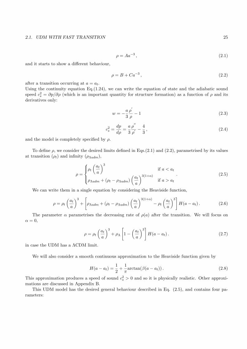
2.1. UDM WITH FAST TRANSITION 25
ρ = Aa−3 , (2.1)
and it starts to show a different behaviour,
ρ = B + Ca−3 , (2.2)
after a transition occurring at a = at.Using the continuity equation Eq.(1.24), we can write the equation of state and the adiabatic soundspeed c2
s = ∂p/∂ρ (which is an important quantity for structure formation) as a function of ρ and itsderivatives only:
w = −a3ρ′
ρ− 1 (2.3)
c2s = dp
dρ= a
3ρ′′
ρ′− 4
3 , (2.4)
and the model is completely specified by ρ.
To define ρ, we consider the desired limits defined in Eqs.(2.1) and (2.2), parametrised by its valuesat transition (ρt) and infinity (ρΛudm),
ρ =
ρt
(ata
)3if a < at
ρΛudm + (ρt − ρΛudm)(ata
)3(1+α)if a > at
. (2.5)
We can write them in a single equation by considering the Heaviside function,
ρ = ρt
(ata
)3+[ρΛudm + (ρt − ρΛudm)
(ata
)3(1+α)− ρt
(ata
)3]H(a− at) . (2.6)
The parameter α parametrises the decreasing rate of ρ(a) after the transition. We will focus onα = 0,
ρ = ρt
(ata
)3+ ρΛ
[1−
(ata
)3]H(a− at) . (2.7)
in case the UDM has a ΛCDM limit.
We will also consider a smooth continuous approximation to the Heaviside function given by
H(a− at) = 12 + 1
πarctan(β(a− at)) . (2.8)
This approximation produces a speed of sound c2s > 0 and so it is physically realistic. Other approxi-
mations are discussed in Appendix B.This UDM model has the desired general behaviour described in Eq. (2.5), and contains four pa-
rameters:

26 CHAPTER 2. UNIFIED DARK MATTER-ENERGY MODELS
at: the scale factor at the transition.
ρt: the value of ρ(a) at a = at.
ρΛudm: the limiting value of ρ(a) at a→∞.
β: parametrising the rapidity of the transition.
Only three of the parameters are independent due to the constraint imposed by the Friedmannequation:
ρt =1−
∑i ρ0,i −
[ρΛudm − ρΛudma
3(1+α)t
]H(1− at)
a3t +
[a
3(1+α)t − a3
t
]H(1− at)
, (2.9)
where the sum is the contribution from the various components of the universe (baryons, photons,neutrinos or any other component). This model has thus two extra parameters (at, β) as compared toΛCDM.
It is important to note that at does not correspond to a time of transition from a DM-like regimeto a DE-like regime. It just defines the time at which the second term of Eq.(2.7) is ”activated”.
We are interested in studying structure formation in the UDM scenario. For the evolution of theperturbations the UDM fluid will follow Eqs.(1.79) and (1.80) or Eqs.(1.85) and (1.86), depending onthe gauge, where the equation of state and the sound speed are those of the UDM fluid.
Starting with the equations (1.75)-(1.80) in the Newtonian gauge, if we combine Eqs.(1.75), (1.77)and (1.78) we obtain an equation for φ
φ′′ + 3H(1 + c2
s
)φ′′ +
(c2sk
2 + 3H2c2s + 2H′ +H2
)φ = 0. (2.10)
On the other hand, if we combine Eqs.(1.75) and (1.76), we obtain the relativistic Poisson equation
k2φ = 4πGa2ρ[δ + 3H (1 + w) θ/k2
]. (2.11)
We can then transform δ of the Newtonian gauge into a gauge independent variable
δ∗ ≡ δ + 3H (1 + w) θ/k2, (2.12)
and the Eq.(2.11) becomes
k2φ = 4πGa2ρδ∗. (2.13)
Using Eq.(2.13) and its derivatives, we obtain an equation for δ∗
δ′′∗ +H(1 + 3c2
s − 6w)δ′∗ −
[32H
2(1− c2
s − 3w2 + 8w)− c2
sk2]δ∗ = 0. (2.14)
To see if δ∗ grows, forming structure, or decays, we can start again from Eq. (2.10). Even if thisequation cannot be solved for an arbitrary equation of state it is possible to derive asymptotic solutions.To do that it is useful to introduce a new variable in order to eliminate the friction term (the termproportional to φ′)

2.1. UDM WITH FAST TRANSITION 27
u ≡ 2φ√ρ+ p
. (2.15)
By expressing H in terms of ρ and p via the conservation law ρ′ = −3H(ρ+ p) we obtain [43]
u′′ + k2c2su−
θ′′
θu = 0, (2.16)
where
θ ≡√
ρ
3(ρ+ p)1a. (2.17)
The solution of Eq.(3.16) may be a growing solution or an oscillatory solution, depending on thescale. The Jeans scale, defined as [40]
k2J ≡
∣∣∣∣ θ′′c2sθ
∣∣∣∣ , (2.18)
is the threshold between the two behaviours. Density contrast will grow on scales larger than kJ andwill not grow efficiently (will oscillate) on smaller scales. Models with large kJ (small scales) are thenthe most favourable to produce structure. Models with a low sound speed (CDM-like) are obviouslyfavourable for structure formation, and as we may have guessed, they have a large value of kJ.
The Jean scale, Eq.(2.18) may be computed as function of the derivatives of ρ, which in turnintroduces dependencies on w and c2
s. After some lenghty calculations we obtain an explicit form fork2
J, (see also, [39])
k2J = 3
2ρa2 (1 + w)
c2s
∣∣∣∣∣12(c2s − w)− ρdc
2s
dρ+ 3(c2
s − w)2 − 2(c2s − w)
6(1 + w) + 13
∣∣∣∣∣ . (2.19)
From this equation we conclude that we can obtain a large k2J, that in principle allows structure
formation, not only when we have a speed of sound equal to zero but also when the speed of soundchanges rapidly. This is the motivation to build UDM models with fast transition.
An important subject to consider when solving numerically the differential equations of the pertur-bations related to each fluid are the initial conditions. Here we will closely follow [7], where we can findan excellent study on cosmological perturbation theory. Numerically, the integration starts at earlytimes, when a given k -mode is still outside the horizon (kτ 1, where kτ is dimensionless), deep in theradiation epoch. At that time, the expansion rate is a/a = τ−1 and massive neutrinos are relativisticand the UDM fluid and the baryons all make a very small contribution to the total energy density(ρt = ργ + ρν). From the differential equations (1.81), (1.83) and the perturbed Boltzmann equation forphotons and neutrinos (which are not described here) we can analytically extract the time-dependenceof the metric and density perturbations on super-horizon scales and end up with the following set ofequations in the synchronous gauge
τ2h′′ + τh′ + 6 [(1−Rν) δγ +Rνδν ] = 0, (2.20)
δ′γ + 43θγ + 2
3h′ = 0, (2.21)

28 CHAPTER 2. UNIFIED DARK MATTER-ENERGY MODELS
θ′γ −14k
2δγ = 0, (2.22)
δ′ν + 43θν + 2
3h′ = 0, (2.23)
θ′ν −14k
2 (δν − 4σν) = 0, (2.24)
σ′ν −215(2θν + h′ + 6η′
)= 0, (2.25)
where Rν ≡ ρν/ (ργ + ρν).For Nν flavour of neutrinos, after the electron-positron pair annihilation and before the massive
neutrinos become nonrelativistic, ρν/ργ = (7Nν/8) (4/11)4/3 is constant.
At first order, and neglecting the terms ∝ k2 in the equations above, we get θ′ν = θ′γ = 0, and theseequations can be combined into a single fourth-order equation for h
τd4h
dτ4 + 5d3h
dτ3 = 0, (2.26)
with four power laws solutions allowing us to obtain the following equations
h = A+B (kτ)−2 + C (kτ)2 +D (kτ) , (2.27)
δ ≡ (1−Rν) δγ +Rνδν = −23B (kτ)−2 − 2
3C (kτ)2 − 16D (kτ) , (2.28)
θ ≡ (1−Rν) θγ +Rνθν = −38Dk. (2.29)
The other metric perturbation η can also be obtained
η = 2C + 34D (kτ)−1 . (2.30)
A general expression for the time depending of the four eigenmodes is derived in [8] and theyshowed that the first two modes (A and B) are gauge modes and can be eliminated by a coordinatetransformation and the other two modes (C and D) are physical modes of density perturbations in theradiation epoch. In the synchronous gauge both appear as growing modes in the radiation epoch butin the matter epoch D decays [13], meaning that the C(kτ)2 mode dominates at later times.
In that sense, we define our initial conditions so that only the fastest growing mode is present andwe obtain the initial conditions at super-horizon-sized perturbations
δγ = −23C(kτ)2, δcdm = δb = 3
4δν = 34δγ , (2.31)
θcdm = 0, θγ = θb = − 118Ck
4τ3, θν = 23 + 4Rν15 + 4Rν
θγ , (2.32)

2.1. UDM WITH FAST TRANSITION 29
σν = 4C3 (15 + 4Rν) (kτ)2 , (2.33)
h = C(kτ)2, η = 2C − 5 + 4Rν6 (15 + 4Rν)C (kτ)2 . (2.34)
And for the Newtonian gauge we obtain
δγ = − 40C15 + 4Rν
= −2ψ, δcdm = δb = 34δν = 3
4δγ , (2.35)
θcdm = θγ = θν = θb = − 10C15 + 4Rν
k2τ = 12k
2τψ, (2.36)
σν = 4C3 (15 + 4Rν) (kτ)2 = 1
15 (kτ)2 ψ, (2.37)
ψ = 20C15 + 4Rν
, φ =(
1 + 25Rν
)ψ. (2.38)
The initial conditions for the UDM fluid are then very straightforward. Since we have all thepotentials as a dependency on the growing mode C, we can replace these potentials in the differentialequations for the UDM fluid in the synchronous or Newtonian gauge. Obtaining, for the Newtoniangauge,
δ′ + 31τ
(c2s − w
)δ = − (1 + w) θ, (2.39)
θ′ +[1τ
(1− 3w) + w′
1 + w
]θ = −k2
(c2s
1 + wδ + 20C
15 + 4Rν
); (2.40)
and for the synchronous gauge
δ′ + 31τ
(c2s − w
)δ = − (1 + w)
(θ + 2Ck2τ
2
), (2.41)
θ′ +[1τ
(1− 3w) + w′
1 + w
]θ = k2 c2
s
1 + wδ. (2.42)
These equations can be simplified by considering that during the radiation epoch, the UDM fluidbehaves exactly as CDM, and we can approximate w = w′ = c2
s = 0, obtaining the CDM initialconditions.

30 CHAPTER 2. UNIFIED DARK MATTER-ENERGY MODELS
2.2 The Generalised Chaplygin Gas
In chapter 3 we shall describe in detail the numerical implementation of the UDM model with a fasttransition. This is the first time that linear structure formation is computed in detail for this particularmodel. As such, there are no previous results with which to compare our results. In order to testif our numerical implementation is well done, we decided to also implement the more widely studiedGeneralised Chaplygin Gas (GCG). Even though the behaviours of the two models are quite different,we can compare the power spectra of the GCG computed with our implementation with published GCGresults, and use it as an indirect test of possible numerical problems in our implementations.
We will now briefly introduce the GCG model. The GCG is defined as a perfect fluid with thefollowing equation of state [33, 44]
pcg = − A
ραcg, (2.43)
where α (ranging from 0 to 1) allows to generalise the standard Chaplygin Gas model, which correspondsto the case α = 0. From the continuity equation (1.24) we get an equation for the evolution of theenergy density of the GCG
ρcg(a) =[A+ a−3(1+α)
(ρ1+αcg(0) −A
)] 11 + α (2.44)
This equation can be rewritten as
ρcg(a) = ρcg(0)[A+ (1− A)a−3(1+α)
] 11 + α . (2.45)
We can see that just like the UDM with fast transition, the GCG has a period (a 1) where
it behaves like DM with ρcg ∝(1− A
) 11+α a−3 and a period (a 1) where it behaves like DE with
ρcg ∝ A1
1 + α (in particular, it can behave like a cosmological constant).
This behaviour is of course expressed also in the evolution of the equation of state, that for theGCG is
wcg = p
ρ= − A
ρ1+αcg
. (2.46)
and in the evolution of the speed of sound
c2s,cg = dp
dρ= −αwcg. (2.47)
The same differential equations (1.79), (1.80), (1.85), (1.86) describe the evolutions of the pertur-bations for this fluid.

2.3. NON-LINEARITY (BACKREACTION) 31
2.3 Non-linearity (Backreaction)
In this thesis we focus on linear perturbations and we will test the model using data on linear scales(see discussion in chapter 4). However, we are aware that in single fluid models the existence of non-linearities also has an impact on the large scale evolution of the universe. This effect, known as theback reaction of small scale clustering onto large scales was studied in [33] for the case of the GCGmodel. This effect arises because as regions of the single fluid collapse and decouple from the evolution,the energy density available to continuing the evolution decreases. This has an impact on both thebackground dynamics of the universe and on the linear clustering. It was shown in [33] that, by alteringthe background evolution, this backreaction may reconcile the original Chaplygin gas model (α = 1)with Supernova data, and, that by altering the oscillations in the linear power spectrum, may reconcilethe GCG model with large-scale structure data.
We implemented backreaction in CLASS for both the GCG model and our fast transition UDMmodel. However, a detailed study of this effect is beyond the goals of this thesis and we do not considerit when testing the UDM model with data in our central analysis. We leave the backreaction resultsand discussion for the appendix.
We followed the idea presented in [33, 44], and considered that the UDM fluid is essentially dividedinto collapsed regions (+) where the energy density is much larger than the average energy density ofthe fluid, and underdense regions (−), that occupy most of the volume of the universe, where the energydensity is smaller than the average.
The average fraction of the total UDM energy E that belongs to collapsed objects (with total energyE+) in a comoving region of the universe of comoving volume V is
ε = E+E. (2.48)
The contribution of the collapsed regions to the average energy density of the universe is
ρ+ = E+V
= ερ, (2.49)
and the contribution from the underdense regions is
ρ− = E−V
= E − E+V
= (1− ε)ρ. (2.50)
The contributions to the pressure come only from the underdense regions, which implies that theeffective equation of state of the fluid is
w = p−ρ
= ρ−ρ
p−ρ−
= (1− ε)w−. (2.51)
The fact that the underdense regions determine the background evolution, but do not contain allthe energy of the fluid, imposes this new effective w and constitutes a backreaction of the collapsedregions on the background evolution.
To completely describe the effect, we need to define the evolution of the fraction ε. We follow [33]and consider the simple model where E+ remains fixed. On the other hand, the total energy evolves asE ∝ ρa−3, and so the evolution of ε is given by

32 CHAPTER 2. UNIFIED DARK MATTER-ENERGY MODELS
ε = ε0ρ0ρa3 , (2.52)
where we introduced the parameter ε0 = ε(a = 1).With ε0 we can now calculate ρ+, ρ− as well as the effective equation of state and the speed of sound
associated with the fluid ρ−. With this, we have all the ingredients needed to compute the perturbationsfor this model including the backreaction. We use the differential Eqs. (1.79), (1.80), (1.85), (1.86),separately for both regions + and −. In particular, for the collapsed regions we use w+ = 0 and c2
s,+ = 0.And for the underdense regions, we use w and cs calculated for the GCG, Eqs.(2.46),(2.47), but nowwith the energy density ρ−.

Chapter 3
Cosmic Linear Anisotropy SolvingSystem (CLASS)
Now that we introduced the UDM and the GCG models, we need a code to allow us to solve the fullset of differential equations for the evolution of perturbations in these models. This will allow us tocalculate the quantities needed to test the models against observables.
In chapter 1, we described the system of perturbed Einstein equations in the Newtonian and syn-chronous gauges for the perturbed energy-momentum tensor of a cosmological fluid. That system ofequations governs the evolution of metric perturbations and contains the fluid equations valid for thematter species. In particular, this system of equations describes linear structure formation in the UDMand GCG models. For radiative cosmological species, such as the CMB photons, the fluid descriptionis not valid and Boltzmann equations must be used [45]. There are a few public cosmological pertur-bations codes available that implement the full set of Einstein-Boltzmann equations. These are usuallyknown in cosmology as Boltzmann codes. Our approach is to implement our models in CLASS [46] bymodifying the Einstein and fluid equations. The UDM and GCG models do not introduce additionalcouplings or modifications in the radiation sector and do not require modifications of the Boltzmanndescription in the code.
The main reason to choose CLASS over other Boltzmann codes such as CAMB [47], CMBFAST[48] or CMBEASY [49] is because CLASS is a new accurate code designed to offer a more user-friendlyand flexible coding environment to cosmologists. CLASS is very well structured, can be modified in aconsistent way, offers a rigorous way to control the accuracy of output quantities, is faster than otherscodes, and is written in C.
A great part of our work relied on the implementation of the UDM model in CLASS to test the modelwith observational data of the inhomogeneous universe. But, as said before, since this implementationis not trivial, we decided to implement in a separate code a GCG model that had been already studiedat perturbation level [44] and compare the results.
Compiling CLASS requires no specific version of the compiler, no special package or library [46].The code is executed with a maximum of two input files, e.g../class explanatory.ini chi2pl1.preThe file with a .ini extension is the cosmological parameters input file, and the one with a .pre extensionis the precision file. Both files are optional: all parameters are set to default values corresponding to the“most usual choices”, and are eventually replaced by the parameters passed in the two input files. For

34 CHAPTER 3. COSMIC LINEAR ANISOTROPY SOLVING SYSTEM (CLASS)
instance, if one is happy with default accuracy settings, it is enough to run with ./class explanatory.ini.Input files do not necessarily contain a line for each parameter, since many of them can be left to defaultvalues. Fig. 3.1 shows part of a modified input file.
Figure 3.1: Part of the input file used to run the UDM model (teste.ini) already with the implementationof the new quantities related to the UDM model.
The code is divided in several modules: one module for the background evolution, one for thethermodynamics, another one for the perturbations, etc. There are no duplicate equations and a givenphysical assumption should be formulated only in a single place. For an illustrative representation ofthe flexibility of CLASS and how it works let us take an example where we integrate over time a setof background and perturbation equations. For the background equations, CLASS uses an adaptiveRunge-Kutta integrator. Such integrators need to be called several times over small time steps. The edgeof these time steps defines the discrete values of time at which background quantities will be tabulatedand stored, in view of being interpolated in other modules. CLASS infers the step sizes automaticallyfrom the rate at which background equations change. So, in a non-standard cosmological model wheresomething special would happen at a given time, the step size would automatically decrease around thattime. The same occurs with the perturbation equations when we use the same Runge-Kutta integrator,which is only an option (the default integrator for perturbations, called ndf15, is described in [50]).
To show how the implementation was made we will follow the flexibility and structure of CLASSand present the implementation for each module separately. Since the code is quite big, we will onlyinclude the most important modules and we will not explain in detail those modules, but rather showthe implementation added in each module and briefly explain its job. Also, it is important to note thatthe implementation of these new fluids was made in a way that allows us to ”activate” or not this newcomponents. If we do not define any parameters of the new fluid, CLASS will set those fluids to zeroand will reproduce the ΛCDM model.

3.1. INPUT MODULE 35
3.1 Input module
The input.c is basically where the code reads the .ini file and goes through a check list of conditionsneeded in order to run the code properly.
We start the implementation by defining a flag for the input parameter Omega lambda udm thatwill activate in case CLASS finds the parameter defined as shown in Fig. 3.2. That flag will tell thecode that we have this fluid in the universe.
Figure 3.2: Part of the code were we define the new flag for the new fluid.
We included the new fluid in some of the conditions of the check list and added new conditions tothe list. As an example, Fig. 3.3 shows the inclusion of the UDM fluid in an already existing conditionto enable to run a model with a DE scalar field.
Figure 3.3: An example of a check where the UDM is now included.
After that we calculate the value of Ωudm today. As we saw in section 2.1, the UDM model isnot parametrised by Ωudm today. We compute this value by subtracting the sum of all other densitycomponents of the cosmological fluid to 1, as shown in Fig. 3.4. In case this does not fill the universecompletely, CLASS completes the sum by adding small amounts of fluids that were not used such asΩΛ, Ωfld, Ωscf and Ωudm (where fld stands for fluid and scf stands for scalar field). This is the generalprocedure used by CLASS to always set the total density to one. We include Ωudm as an availablechoice for CLASS users by including the lines of code shown in Fig. 3.5.
Figure 3.4: Calculating Ω0,udm.

36 CHAPTER 3. COSMIC LINEAR ANISOTROPY SOLVING SYSTEM (CLASS)
Figure 3.5: Filling the universe in case the sum of all densities does not equal unity.
Another important modification is the inclusion of the lines of code shown in Fig. 3.6, that allowsCLASS to read the values of the UDM parameters and backreaction parameters defined in the inputfile.
Figure 3.6: Reading the values of the UDM and backreaction parameters from the input file.
Figure 3.7: The default value of each new parameter is defined in case they are not expressed in theinput file.
Similar to what is done for all other components, we also define default values for the new parameters

3.2. BACKGROUND MODULE 37
in case the user does not define them in the input file. In the example shown in Fig. 3.7 we set thedefault value of Ωudm to zero, meaning that the code will run ΛCDM if we do not assign any value forthis parameter in the input file.
3.2 Background module
At background level, we introduced the new fluid in CLASS as a new component that can enter theHubble function. This modification involves the introduction of new quantities in the background struc-ture (background.h), and in the background module (background.c).
The background structure, as all structures of other modules, is where we define the quantities thatwe need to store and pass from one module to another, including flags, variables and vectors.
We start by calculating the value of Ωudm at the time of the transition. We define it as ρtρcrit,0,using the critical density of today as normalisation. Then we define how the energy density of the UDMfluid evolves Eq.(2.6) as well as the other important quantities related to the fluid, like the equation ofstate Eq.(2.3) and the speed of sound Eq.(2.4). Also, we define a matter-like part of the UDM fluid,ρm,udm, as
ρm,udm = ρt
(ata
)3. (3.1)
This means that the UDM fluid was purely matter-like behaviour before the transition, and after thetransition this evolving density will be considered as a matter component of the UDM. The remainingdensity, ρudm − ρm,udm, will be considered as the dark energy component of the UDM, ρDE,udm. Thecomputation of all these quantities is shown in Fig. 3.8.
Figure 3.8: Part of the code in background.c module where ρ, w and c2s for the UDM model were
implemented.
After we defined these background equations we verify whether we want to consider backreaction

38 CHAPTER 3. COSMIC LINEAR ANISOTROPY SOLVING SYSTEM (CLASS)
or not. In case we do not want to, we add the energy density of the UDM to the total energy density,as well as the pressure. When backreaction is considered, we separate the energy density in a part thatbelongs to collapse regions and a part that belongs to underdense regions and re-calculate the speedof sound and the equation of state as discussed in section 3.3. After these considerations, we can thenproceed to modify the Hubble function, as shown in Figs. 3.9 and 3.10.
Figure 3.9: Including UDM energy density and pressure in the Hubble function without backreaction.
Figure 3.10: Including UDM energy density and pressure in the Hubble function considering the back-reaction effect.
Upon running, the code outputs some information on-screen, that now has UDM-related informa-tions, and an output data file showing the evolution of various background quantities, such as the Hubblefunction and various cosmological distances and densities, against redshift. Besides UDM-related quan-tities, we have also included the scale factor in the output file, which is a convenient time variable,
related to the redshift as a = 1z + 1 . The various steps needed to modify the outputs are shown in Figs.
3.11, 3.12 and 3.13.

3.2. BACKGROUND MODULE 39
Figure 3.11: Including on-screen information related to the UDM.
Figure 3.12: Adding new columns and their titles in the background data file.
Figure 3.13: Filling the UDM-related columns.
3.2.1 Results
The implementation of the UDM model at background level already allows us to study some of itsproperties.
Fig. 3.14 shows the evolution of the densities of the various fluids present in this cosmology. Wecan notice that the density of radiation decreases faster than the density of matter or the UDM, justlike in ΛCDM, and that the UDM decreases first with the same rate as the baryons but later graduallydeviates (when the transition takes place) and approaches the critical density. It is also important tonote, as mentioned in section 2.1, that in this example at = 0.01, but the scale factor at which theUDM fluid is dominated by the DE-like density (ρDE,udm = ρudm − ρm,udm) is a∗ ∼ 0.714.

40 CHAPTER 3. COSMIC LINEAR ANISOTROPY SOLVING SYSTEM (CLASS)
Figure 3.14: Plot of the evolution throughout time (redshift) of the energy densities of the variouscomponents present in this cosmological model. The UDM fluid is characterised by at = 0.01, β = 5×10⁴
and ΩΛudm = 0.7. The components are radiation (rho g, blue line), baryons (rho b, orange) and UDM(rho udm, green). The evolution of the critical density is also shown (rho crit,red).
By adding the c2s and w evolution to the output data file, we can make comparisons with the results
of [41], as shown in Figs. 3.15 and 3.16. In both cases, there is a perfect match.
In Fig. 3.16 notice that the evolution of ρ(a)ρΛ is a monotonic decreasing function and can beused as a time variable. In this model, the transition is at at ∼ 0.2 and the value ρρΛ = 50 correspondsto ρ = ρt, showing that the peak in the sound speed occurs at the transition a = at. In our results,shown as function of redshift, the peak occurs at zt ∼ 4, or at ∼ 0.2 and the two results match perfectly.

3.2. BACKGROUND MODULE 41
Figure 3.15: Comparison of the evolution of the equation of state w obtained with our CLASS imple-mentation (left panel) with the results of [41] (right panel).
Figure 3.16: Comparison of the plot obtained with the output data file of the background module (left)with the one presented in Ref. [41] (right) of the evolution of the c2
s. Right panel uses the density as atime variable, since its evolution is monotonic. ρ/ρΛ = 50 corresponds to ρ = ρt showing that the peakoccurs at the transition a = at. The transition occurs at at ' 0.2 ⇔ zt ' 4, and the 2 panels matchperfectly.

42 CHAPTER 3. COSMIC LINEAR ANISOTROPY SOLVING SYSTEM (CLASS)
Figure 3.17: Implementation of a test to forbid sound speeds greater than one.
It is also important to note that after the transition the sound speed does not actually go to zero butto values very close to it. This remaining sound speed, even if very small, could have a large influenceon the evolution of perturbations. We will address this issue in Appendix B.
Figure 3.18: Evolution of the speed of sound for the models: (at = 0.05, β = 100 and ΩΛudm = 0.7;blue), (at = 0.01, β = 500 and ΩΛudm = 0.7; orange), (at = 0.001, β = 1000 and ΩΛudm = 0.7; green).In these cases, the sound speed does not go to zero as the universe evolves.
Fig. 3.18 shows the evolution of the speed of sound for three models that produce sound speedpeaks of low amplitude at the transition. In those cases the speed of sound does not drop to zeroafter the transition but increases again. This is a feature of the Heaviside approximation and it ismost proemient in models with low amplitude peaks. Other choices of Heaviside approximations arediscussed in Appendix B.
3.3 Perturbation module
In the perturbation module, as in every module, we add the UDM-related variables in the perturbationheader (perturbation.h). These are δudm and θudm or δ+,udm,δ−,udm, θ+,udm, θ−,udm in the case of back-reation. In the file perturbation.c we check the flags that tell us if we want to consider perturbations inthe UDM fluid and backreaction. According to that, we add the evolution of the relevant perturbationsfor the UDM fluid in the output file of perturbations as shown in Fig. 3.19. Those quantities are alsopassed on to the next modules.
Then, we define the initial conditions. In CLASS, the initial conditions for photons are computedfrom the matter components according to the standard prescription derived in section 3.1. This is the

3.3. PERTURBATION MODULE 43
major reason why we needed to define a matter-like component of the UDM fluid. We add then thiscomponent, ρm,udm to the total ρm, which is used to define others quantities that will be used to definethe initial condition of the photons. From the initial conditions for the photons we add the initialconditions for the UDM fluid with and without backreactions using the equations defined in section 3.1.Fig. 3.20 shows the inclusion of these conditions for the case of the synchronous gauge.
Figure 3.19: Part of the code where new column titles for UDM perturbations are added.
Figure 3.20: Part of the code where we define the initial conditions for the UDM fluid in the synchronousgauge.
Figure 3.21: Part of the code where we include the UDM fluid in the gauge transformation variables.

44 CHAPTER 3. COSMIC LINEAR ANISOTROPY SOLVING SYSTEM (CLASS)
To have the possibility to compute UDM perturbations in the Newtonian gauge, we also implementedthe gauge transformation equations for the UDM fluid (see Fig. 3.21) and the corresponding initialconditions (see Fig. 3.22).
Figure 3.22: Part of the code where we define the initial conditions for the UDM fluid in the Newtoniangauge.
We arrive now to the point of adding the UDM perturbations to the total perturbed energy mo-mentum tensor. This is shown in Fig. 3.23.
Figure 3.23: Part of the code where we add the contribution of the UDM perturbations to the totalperturbed energy-momentum tensor.
We can now include in CLASS the differential equations of the perturbations for the UDM fluidfor the two implementations, with or without backreaction. These are Eqs. (1.79), (1.80), (1.85) and(1.86). The new lines of code are shown in Figs. 3.24 and 3.25.

3.3. PERTURBATION MODULE 45
Figure 3.24: Part of the code where we add the differential perturbative equations for the UDM fluidwithout backreaction.
Figure 3.25: Part of the code where we add the differential perturbative equations for the UDM fluidwith backreaction.
The central quantity to study the large scale structure in the universe, and the one we will use to testthe models against data, is the matter power spectrum. To test the UDM model, besides computing theevolution of all of its perturbed quantities, we also need to define what its contribution is to the total

46 CHAPTER 3. COSMIC LINEAR ANISOTROPY SOLVING SYSTEM (CLASS)
matter perturbations δm, the basis of the matter power spectrum. We did a similar choice at backgroundlevel, when we defined a ρm,udm. Here, at perturbative level, we follow the approach suggested in [42]and consider that the matter-like contribution of the UDM density contrast δudm is the fraction
δm,udm = ρudmδudmρm
. (3.2)
In Fig. 3.26 we can see the lines of code where we add the matter-like contribution of the UDMdensity contrast to the total δm.
Figure 3.26: Part of the code where we add the contribution of the UDM perturbations to the δm, usedlater to calculate the matter power spectrum.
3.3.1 Results: evolution of the density contrast
With the implementation of this module finished we can now compute the evolution of the densitycontrast and the divergence velocity for the UDM fluid and observe some general behaviours that arecharacteristic of the model.
As an example, we look at the evolution of δudm for different values of the parameters of the modeland compare it with the evolution of δcdm in ΛCDM. Figs. 3.27, 3.28 and 3.29 show the evolutions forthree different scales.

3.3. PERTURBATION MODULE 47
Figure 3.27: Evolution of δudm for a large scale k = 0.01 for different values of the model parameters:orange: ΩΛudm = 0.70, βudm = 200, atransition = 0.17; green: ΩΛudm = 0.5, βudm = 200, atransition =0.17; red: ΩΛudm = 0.70, βudm = 200, atransition = 0.05; violet: ΩΛudm = 0.70, βudm = 10, atransition =0.11; brown: ΩΛudm = 0.70, βudm = 100, atransition = 0.3; pink: ΩΛudm = 0.70, βudm = 5 × 10⁵,atransition = 0.01; blue: δcdm in a flat ΛCDM model with ΩΛ = 0.70.
Figure 3.28: Evolution of δudm for a intermediate scale k = 0.1 for different values of the modelparameters: orange: ΩΛudm = 0.70, βudm = 200, atransition = 0.17; green: ΩΛudm = 0.5, βudm = 200,atransition = 0.17; red: ΩΛudm = 0.70, βudm = 200, atransition = 0.05; violet: ΩΛudm = 0.70, βudm = 10,atransition = 0.11; brown: ΩΛudm = 0.70, βudm = 100, atransition = 0.3; pink: ΩΛudm = 0.70, βudm =5× 10⁵, atransition = 0.01; blue: δcdm in a flat ΛCDM model with ΩΛ = 0.70.

48 CHAPTER 3. COSMIC LINEAR ANISOTROPY SOLVING SYSTEM (CLASS)
Figure 3.29: Evolution of δudm for a small scale k = 10 for different values of the model parameters:orange: ΩΛudm = 0.70, βudm = 200, atransition = 0.17; green: ΩΛudm = 0.5, βudm = 200, atransition =0.17; red: ΩΛudm = 0.70, βudm = 200, atransition = 0.05; violet: ΩΛudm = 0.70, βudm = 10, atransition =0.11; brown: ΩΛudm = 0.70, βudm = 100, atransition = 0.3; pink: ΩΛudm = 0.70, βudm = 5 × 10⁵,atransition = 0.01; blue: δcdm in a flat ΛCDM model with ΩΛ = 0.70.
We notice that the free parameters of the UDM model have a strong influence on the evolution ofthe density contrast and also that the same parameter’s values give different features for the densitycontrast on different scales.
In these figures we try to provide a wide range of possibilities for the evolution of the density contrastof UDM in those three scales by choosing several combinations of the parameter values. We try to showthe impact of each parameter by fixing two parameters and changing only one. For example, from theorange curve to the green one we only change the parameter ΩΛudm and we see that at k = 0.01 thedensity contrast for the green curve is always very close to zero while for the orange curve there is astrong deviation from zero. However at k = 0.1 the green curve shows a strong oscillatory solution incomparison to the orange one that now tends much faster to zero.
We also try to show the differences between a very early and very fast transition (pink curve) anda slower and late transition (violet and brown curves). In those cases we observe that the pink curvefollows closer the δcdm at k = 0.01 in comparison to the other cases, especially comparing with thebrown curve where we observe a huge oscillation. At k = 0.1 we still see a good behaviour for the pinkcurve while the other two are already oscillating very close to zero, suggesting that with this choice ofparameters the evolution of δudm strongly decays with the scale. At the small scale k = 10 we now seea strong oscillation for the pink curve and the other two cases have δudm = 0.
We can also compare a case with an early and fast transition (pink curve) with an early and slowertransition (red curve). We see that both cases show the same behaviour at k = 0.01, but at the othersscales, k = 0.1 and k = 10, the red curve δudm tends to zero. These comparisons give us an indicationthat a UDM model with a very fast and early transition could result in a promising matter powerspectrum.

3.3. PERTURBATION MODULE 49
We also find a general behaviour in all the cases. At all scales, the UDM fluid follows the ΛCDMmodel until the transition takes place and after that, we observe an oscillatory solution in all cases.These oscillations are very different from model to model and they are of course related to the soundspeed being different from zero. In some cases, the oscillations are very large. This does not happenin our control model, the GCG, where in Fig. 3.30 and in the results of Appendix A we can see thatthe density contrast also follows ΛCDM until the transition and then starts to oscillate but with smalloscillations.
The results for the GCG model, shown in Appendix A, are in perfect agreement with the resultspublished in [44], and successfully validate our implementation procedure in CLASS. However theremight be some numerical problems with the UDM implementation, not shown by this test. Numerically,the main difference between the two models is the fact that the speed of sound may be very peaked inthe UDM model with fast transition. We need to be sure that the large oscillations found are truly afeature of the model and are not due to some numerical problem related to the numerical integrationof a strongly peaked function.
Figure 3.30: Evolution of δGCG and δcdm over time for the large scale k = 0.01, for A chap=0.72 andα = 0.2.
We made two different consistency tests to verify our solutions of δ. The first test was to use aRunge-Kutta integrator as an alternative to the ndf15 numerical integrator used by default in CLASS.The second test was to use a different continuous approximation to the Heaviside function, to see theimpact on the oscillatory pattern. In both tests we found no significant difference from the previousresult, and we consider our UDM results to be reliable for model testing and will use them in the nextchapter. As a side product of the second test, we found that some of the Heaviside approximationsused (the sigmoid functions) allow for some interesting physical properties. We discuss this point inAppendix B.

50 CHAPTER 3. COSMIC LINEAR ANISOTROPY SOLVING SYSTEM (CLASS)
3.4 Other modules
After finishing this module we have the implementation almost complete. Now, we only need to modifytwo more modules: spectra.c and thermodynamics.c. The first one will allow us to calculate the desiredmatter power spectrum and the angular power spectrum for the CMB. On the second one, we addedthe UDM fluid to be part of the matter sector of the universe that is passed to the two recombina-tions codes that are integrated with CLASS (RECFAST and HyRec). It is important to note thatfurther modifications would be needed if we wanted for example to consider models with dark matterannihilation.
3.4.1 Results: power spectra
With these last implementations we obtain all the desired quantities to test our model. In Fig. 3.31 weshow the CMB temperature angular power spectrum.This power spectrum is very sensitive to ΩΛ, or more precisely to Ωm due to the flatness condition.Shallower potential wells allow for large oscillations in the baryon-photon plasma and so models withless matter (large ΩΛ) such as the green model in Fig. 3.31 has larger amplitude than smaller ΩΛ models(orange).
Figure 3.31: Temperature angular power spectrum of the CMB for different values of the model pa-rameters: green: ΩΛudm = 0.70, βudm = 200, atransition = 0.17; orange: ΩΛudm = 0.5, βudm = 200,atransition = 0.17; red: ΩΛudm = 0.70, βudm = 5× 10⁵, atransition = 0.01; blue: flat ΛCDM model withΩΛ = 0.70.
The CMB power spectrum is also sensitive to the UDM at and β parameters. The model in red, inFig. 3.31, shows a UDM model with early and fast transition that produces a CMB power spectrumvery similar to ΛCDM.
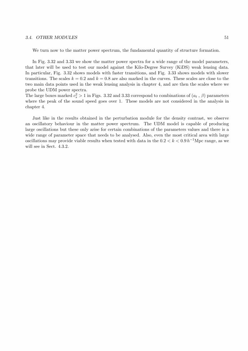
3.4. OTHER MODULES 51
We turn now to the matter power spectrum, the fundamental quantity of structure formation.
In Fig. 3.32 and 3.33 we show the matter power spectra for a wide range of the model parameters,that later will be used to test our model against the Kilo-Degree Survey (KiDS) weak lensing data.In particular, Fig. 3.32 shows models with faster transitions, and Fig. 3.33 shows models with slowertransitions. The scales k = 0.2 and k = 0.8 are also marked in the curves. These scales are close to thetwo main data points used in the weak lensing analysis in chapter 4, and are then the scales where weprobe the UDM power spectra.The large boxes marked c2
s > 1 in Figs. 3.32 and 3.33 correspond to combinations of (at , β) parameterswhere the peak of the sound speed goes over 1. These models are not considered in the analysis inchapter 4.
Just like in the results obtained in the perturbation module for the density contrast, we observean oscillatory behaviour in the matter power spectrum. The UDM model is capable of producinglarge oscillations but these only arise for certain combinations of the parameters values and there is awide range of parameter space that needs to be analysed. Also, even the most critical area with largeoscillations may provide viable results when tested with data in the 0.2 < k < 0.9h−1Mpc range, as wewill see in Sect. 4.3.2.

52 CHAPTER 3. COSMIC LINEAR ANISOTROPY SOLVING SYSTEM (CLASS)
Figure 3.32: Matter power spectrum for a fixed value of ΩΛudm = 0.7 and for at =0.001, 0.01, 0.05, 0.1, 0.15, 0.2, 0.3, 0.5, 0.7, 0.9, 1.5, increasing from the bottom to the top and for val-ues of βudm = 103, 5 × 10³, 104, 5 × 10⁴, 105, 5 × 10⁵, increasing the speed of the transition from theright to the left.

3.4. OTHER MODULES 53
Figure 3.33: Matter power spectrum for a fixed value of ΩΛudm = 0.70 and for at =0.001, 0.01, 0.05, 0.1, 0.15, 0.2, 0.3, 0.5, 0.7, 0.9, 1.5, increasing from the bottom to the top and for val-ues of βudm = 0.1, 1, 10, 50, 100, 500, increasing the speed of the transition from the right to theleft.

54 CHAPTER 3. COSMIC LINEAR ANISOTROPY SOLVING SYSTEM (CLASS)

Chapter 4
Testing cosmological models
After the implementation of the model it is time to test it with several quantities that can be observedand used to constrain the parameters space of the model.
In this chapter we start by presenting the current constraints on the UDM model based on back-ground tests. Then we will present the analysis made in this dissertation, where we test the model firstwith a combination of SNe Ia, BAO and CMB data, and later by introducing structure formation usingweak lensing data.
4.1 Background tests
The UDM model that we study in this dissertation was already tested at background level in [51].There, the authors used a combination of data related with quantities obtained in the homogeneousstudy of the model. They used two background features of CMB data, which are the scaled distance tothe photon-decoupling surface
R ≡√
ΩmH20r(z∗)c
, (4.1)
and the angular scale of the sound horizon at the photon-decoupling epoch
la ≡ πr(z∗)rs(z∗)
, (4.2)
where r(z∗) is the comoving distance to the photon-decoupling surface lying at redshift z∗ and rs(z∗) isthe comoving sound horizon at z∗. These quantities are measured in the CMB observations, for examplela is the scale of the first peak in the CMB power spectrum, and can be calculated for the UDM modelas a function of its parameters, allowing to estimate the parameter values and test the model.
In [51], they also used BAO data, which depend on H(z)rs(zd)/c and DA (angular diameter dis-tance). Finally, they also used SNe Ia data which provide the distance modulus, which is a quantitythat can be computed theoretically for the UDM model.
µ(z) = 5 log10 dL(z) + µ0 , (4.3)

56 CHAPTER 4. TESTING COSMOLOGICAL MODELS
Model h Ωc Ωb at β ΩΛ χ2red lnBiΛ
UDM 0.69508+0.00068−0.00064 0.2445+0.00011
−0.00012 0.04626+0.00024−0.00026 0.17+0.010
−0.011 552+75−69 0.7091+0.0015
−0.0013 0.9501 +0.791ΛCDM 0.6906+0.0090
−0.0093 0.245+0.011−0.010 0.0462+0.00097
−0.00096 – – 0.708+0.011−0.012 0.9488 0
Table 4.1: Summary of the constraints (median values and 1-σ intervals) for the model parametersusing CMB, BAO and SN data. The minimum reduced χ2 and the Bayes factor with respect to ΛCDMare also shown.
where dL is the luminosity distance that can be computed from
dL(z) = (1 + z)∫ z
0
dz′
E(z′) . (4.4)
In their analysis, the model was found to fit the data as well as the concordance model does.The Bayes factor is the ratio between the evidences of two models and is a criteria to make modelselection. We see in Tab. 4.1 that the UDM model is slightly preferred over the ΛCDM model, witha small positive value of the logarithm of the Bayes factor, despite having two extra parameters. Wecan also see that the estimated values for the UDM parameters are a scale factor at a value for thetransition of at = 0.17, corresponding to a redshift zt = 4.9, and β = 552. These parameters wereestimated with a good precision of 6 % and 13 % respectively.
Thus, at background level this model is a viable alternative to explain the late accelerated expansionof the universe.
4.2 Tests in the inhomogeneous universe
Now, we will describe the analysis performed in this dissertation, concerning the tests at perturbationlevel. For that, we will start by introducing the structure formation observable that we used (weakgravitational lensing). Then we will show the analysis procedure and in particular the Markov ChainMonte Carlo (MCMC) code that we used (MontePython), for parameter estimation. There are twomain parts in the code, the algorithm for sampling the parameters space and the likelihood codes ofthe various datasets.Finally, we present the results.
4.2.1 Weak gravitational lensing
Cosmological weak gravitational lensing, also known as cosmic shear, is the deflection of photons pathscaused by inhomogeneities in the universe where the photons propagate. The photons are emitted byastrophysical sources such as galaxies, and this lensing effect is caused by the variation of density, andtherefore by the gravitational potentials, that exist along the propagation path. In that way, cosmicshear is a way to learn more about the distribution of matter in the universe. Since cosmological modelsmake predictions of how matter is distributed in the universe, cosmic shear is then an excellent tool todiscover the best model for the universe.
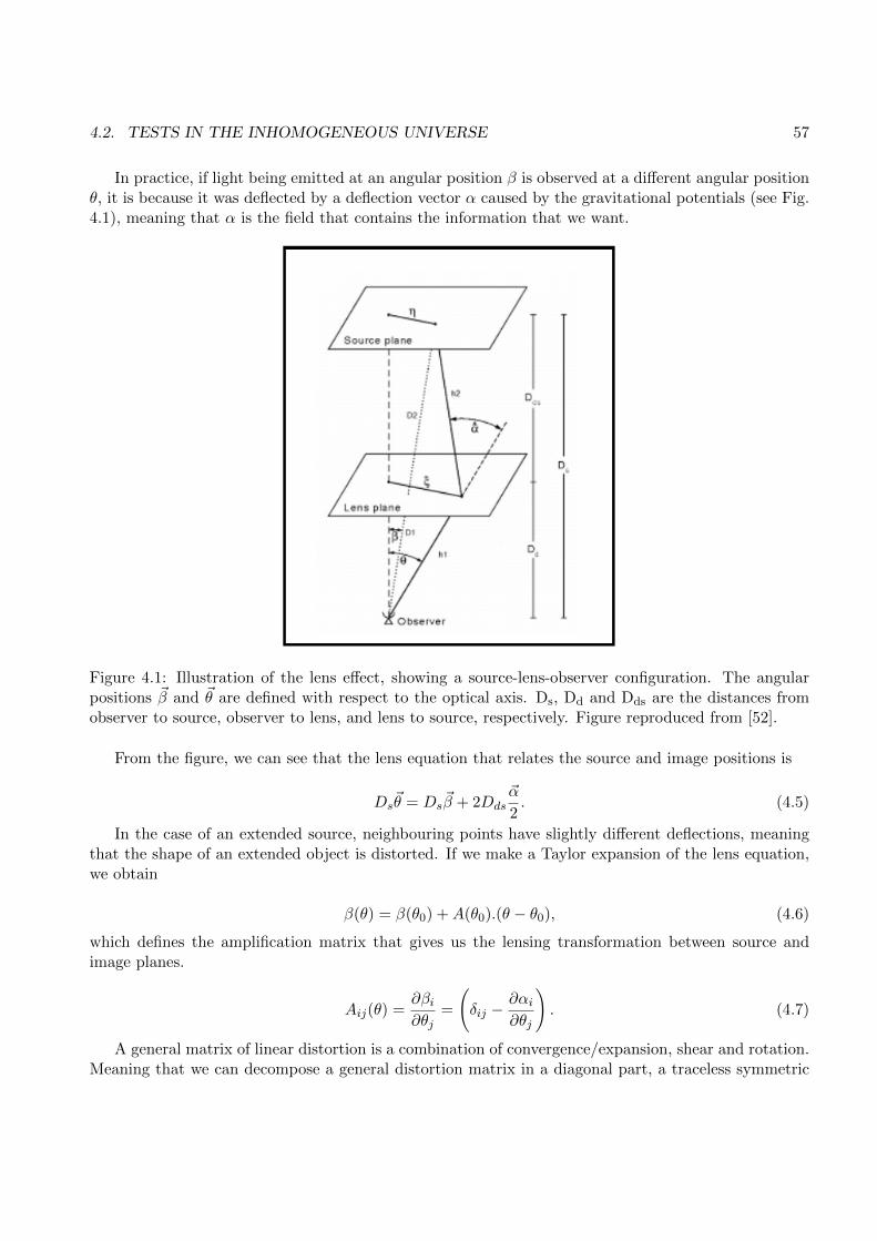
4.2. TESTS IN THE INHOMOGENEOUS UNIVERSE 57
In practice, if light being emitted at an angular position β is observed at a different angular positionθ, it is because it was deflected by a deflection vector α caused by the gravitational potentials (see Fig.4.1), meaning that α is the field that contains the information that we want.
Figure 4.1: Illustration of the lens effect, showing a source-lens-observer configuration. The angularpositions ~β and ~θ are defined with respect to the optical axis. Ds, Dd and Dds are the distances fromobserver to source, observer to lens, and lens to source, respectively. Figure reproduced from [52].
From the figure, we can see that the lens equation that relates the source and image positions is
Ds~θ = Ds
~β + 2Dds~α
2 . (4.5)
In the case of an extended source, neighbouring points have slightly different deflections, meaningthat the shape of an extended object is distorted. If we make a Taylor expansion of the lens equation,we obtain
β(θ) = β(θ0) +A(θ0).(θ − θ0), (4.6)
which defines the amplification matrix that gives us the lensing transformation between source andimage planes.
Aij(θ) = ∂βi∂θj
=(δij −
∂αi∂θj
). (4.7)
A general matrix of linear distortion is a combination of convergence/expansion, shear and rotation.Meaning that we can decompose a general distortion matrix in a diagonal part, a traceless symmetric

58 CHAPTER 4. TESTING COSMOLOGICAL MODELS
and a traceless antisymmetric part, respectively.
A =[k 00 k
]+[γ1 γ2γ2 −γ1
]+[
0 w−w 0
]We need to see how to relate the deflection field ~α with the deflection potential. Let us consider
that the light that comes from the source passes then through a local potential φ. The potential canbe included as a scalar perturbation in the FLRW metric, as we saw in section 1.2
ds2 = − (1 + 2φ) dt2 + (1− 2φ)[dx2
1 + dx22 + dx2
3
]. (4.8)
Let us consider photon trajectories in this metric. From the equation of geodesic deviation we canfind the following differential equation for the separation vector (~x) between the photon trajectory andthe optical axis, as function of comoving radial distance w [52]
d2~x
dw2 +K~x = −2[~∇⊥φ
(~x(~θ, w
), w)− ~∇⊥φ (0, w)
], (4.9)
where K is the curvature of the universe. This shows that the separation vector, and consequently thedeflection, depends on the gradient of the potential in the plane orthogonal to the trajectory (meaningin the lens plane).
The equation has the following solution
~x(~θ, w
)= fK(w)~θ − 2
∫ w
0dw′fK(w − w′)
[~∇⊥φ
(~x(~θ, w
′), w′)− ~∇⊥φ
(0, w′
)]. (4.10)
We can write this solution in terms of angular positions
βi(~θ, w
)= θi − 2
∫ w
0dw′ fK
(w − w′
)fK (w) fK
(w′) [
φ,i(~x(~θ, w
′), w′)− φ,i (0, w′
)]. (4.11)
This has exactly the structure of the lens equation Eq. (4.5), telling us that the second term of theright-hand side is the solution for the deflection as a function of the potential. where the second term isthe solution for the deflection as a function of the potential. This shows that the total deflection is theintegral over all local deflections, each one multiplied by a ‘weight’ or efficiency factor that is essentially
DdsDd
Ds. (4.12)
From Eqs. (4.7) and (4.8), we know that the spatial derivatives of the deflection field define theoptical scalar fields, the elements of the amplification matrix. We see then that they are second-orderderivatives of an effective cosmological lensing potential defined as
ψ(~θ, w
)= 2
∫ w
0dw′ fK
(w − w′
)fK (w) fK
(w′)φ(fKθ, w
′). (4.13)
With this definition we can write the optical scalars as

4.2. TESTS IN THE INHOMOGENEOUS UNIVERSE 59
convergence
k = 12 (ψ,11 + ψ,22) . (4.14)
shear
γ1 = 12 (ψ,11 − ψ,22) , γ2 = ψ,12, (4.15)
and rotation
w = 0. (4.16)
The convergence k in Eq. (4.14), is the Laplacian of a potential and can be related with the massof the lens through the Poisson equation
∇2pφ = 4πGρδ = a24πGΩmρca
−3δ = 3H20 Ωmδ
2a . (4.17)
This allows us to obtain the dependency of the lensing optical scalars fields on the density contrastfield
k(~θ, w
)= 3
2H20 Ωm
∫ w
0dw′ fK
(w − w′
)fK(w′)
fK (w) a (w′) δ(fK(w′) ~θ, w′) . (4.18)
This is the convergence field produced by the lenses δ(w′) located in the comoving distance rangew′ ∈ [0, w]. They affect the image of a single source located at w. In practice there is not a singlesource but a distribution of source galaxies that are distributed over redshift, between 0 and a maximumpossible distance wH .The convergence then becomes
k(~θ)
= 32H
20 Ωm
∫ wH
0dw′ fK
(w′)
a (w′) δ(fK(w′) ~θ, w′) g (w′) , (4.19)
with
g(w′) =
∫ wH
wdw p (w)
fK(w − w′
)fK (w) (4.20)
being the contribution weight of each source galaxy w′ that belongs to the source redshift distributionp(w). The power spectrum of the convergence field is then related to the matter power spectrum
Pk (l) = 94H
40 Ω2
m
∫ wH
0dw
g2 (w)a2 (w)Pδ
(l
fK (w) , w). (4.21)
That means that if our model predicts a certain Pδ we can also compute the Pk that will correspondto a certain source distribution.
Since the convergence field and the shear field are second-order derivatives of the cosmological lensingpotential, they are related. It is easy to compute their relation in the Fourier space, which is,

60 CHAPTER 4. TESTING COSMOLOGICAL MODELS
γ(~l)
=(l21 − l22 + 2il1l2
l2
)k(~l), (4.22)
and implies that their power spectra are identical
Pγ (l) = Pk (l) . (4.23)
This procedure allows us to relate the matter power spectrum to the convergence power spectrum,to the shear power spectrum and to the shear correlation function. The shear correlation function orpower spectrum are the quantities usually computed from measurements of ellipticity of galaxies inweak lensing surveys. This then allow us to compare our theoretical calculation of the shear powerspectrum with the observed ones and compare them and test our model.It is important to note that this procedure allows us to compute the linear power spectrum. However,on small scales (k > 0.2hMpc−1) the dark matter density contrast is large and non-linear correctionsmay be needed.
The regime where the non-linearity starts depends on the model and how fast or slow the structureforms, however we expect that any model will require some level of non-linear corrections. To solve thisproblem what is usually done is to use of N-body simulations that allow us to evolve the model startingfrom a time where the power spectrum is still linear at all scales. These simulations demand heavycomputation and what is common to do, for example in the ΛCDM, is to evolve the system for certainparameter values and from these simulations extrapolate a fitting function that allows to correct thelinear power spectrum in the non-linear regime [53].
4.2.2 KiDS Survey
The Kilo-Degree Survey (KiDS) is an ongoing ESO optical survey that will try to cover 1350 deg2 ofthe extragalactic sky in four bands (u,g,r,i). It uses the OmegaCAM CCD mosaic camera mounted atthe Cassegrain focus of the VLT Survey Telescope (VST). This combination of camera and telescopewas specifically designed for the weak lensing studies [54, 55].
A weak lensing cosmological survey measures the ellipticity of the image galaxies. The ellipticity isa two component polar vector with a modulus describing the deviation from circularity and a direction.In the weak lensing approximation, where the optical scalars are small, the observed ellipticity is infact the sum of two features: the intrinsic ellipticity of the galaxies plus the shear caused by the lensingpotential [52], γob = γs + γcosmo. The intrinsic ellipticities of galaxies are not necessarily independentbecause the orientations of galaxies are determined by physical processes that could produce correlatedintrinsic alignments. For this reason the correlation function measured by KiDS is
〈γobγob〉 = 〈γcosmoγcosmo〉+ 〈γcosmoγs〉+ 〈γsγcosmo〉+ 〈γsγs〉. (4.24)
The terms 〈γcosmoγs〉, 〈γsγcosmo〉 and 〈γsγs〉 are three types of intrinsic alignments, while 〈γcosmoγcosmo〉is the shear correlation function containing the cosmological information. This equation is then a biasedestimator of the shear correlation function.
In our analysis we have used the KiDS-450 dataset where the galaxies ellipticities were measuredusing 450 deg2 of imaging data. From the observed ellipticities, the KiDS team computed the ellipticitycorrelation function 〈γcosmoγcosmo〉 and the ellipticity power spectrum with a quadratic estimator. This

4.3. ANALYSIS 61
was done separating the source galaxies in three redshift bins (zbins: 0.1− 0.3, 0.3− 0.6 and 0.6− 0.9),producing five different shear power spectrum spectra and correlation functions (bin1-bin1, bin2-bin1,bin2-bin2, bin3-bin3, bin1-bin3), each of the five power spectra measured on angular scales rangingfrom l = 76 to l = 1310.We will work with the publicly available shear power spectra and will use the public likelihood codeprovided in [55].
To compute the likelihood of our UDM model given these KiDS data we will need to specify notonly the cosmological parameters values, but also six extra (nuisance) parameters that account for thebias in the measurements. These are: the 3 parameters A noise z1,2,3 that represents the uncertaintyassociated to the 3 redshift bins of the galaxies. The m corr parameter that represents the uncertaintyon the calibration of the ellipticity measurement of the galaxies. The A IA parameter that representsthe uncertainty in the amplitude of the intrinsic alignment effect. The A bary parameter allows for anuncertainty on the dark matter power spectrum amplitude due to feedback from baryons. Also, thelikelihood code by default already accounts for the uncertainty in the n(z) distribution of galaxies byrandomly choosing one of one thousand realisations.
4.3 Analysis
4.3.1 MontePython
MontePython is a Monte Carlo code for Cosmological Parameter extraction. It is prepared to workintegrated with CLASS and contains already several likelihood codes for the most recent experiments[56]. It includes several methods to sample the parameter space: Metropolis-Hastings [57], NestedSampling [58, 59] (through MultiNest [60]), EMCEE [61] (through CosmoHammer [62]) and ImportanceSampling.
In our analysis we will mostly use the Metropolis-Hastings algorithm, which is a Markov Chain MonteCarlo (MCMC) method. In this method, points in the parameter space are generated in sequence froman auxiliary proposal distribution. Each point may be accepted or rejected by evaluating its likelihoodagainst the data and comparing it with the likelihood of the previous point. The algorithm is designedsuch that the sequence of points mainly moves towards regions of higher likelihood, probing those regionswith higher resolution. The chain of points formed is called a Markov chain because each point dependson the previous point of the chain. When the process is finished, the resulting chain is a representativesample of the probability distribution in the parameters space.
Running the code is very straightforward. After defining several configurations, we are ready to useit. MontePython comes with only two main commands. The first one is used to run a chain and thesecond one reads the chains and produces several outputs such as covariant matrices, plots or bestfitvalues. To see the list of arguments available in each command all we need to do is type ”pythonmontepython/Montepython.py run -h/–help” for the run, and ”python montepython/Montepython.pyinfo -h/–help” for analysing the chain.
To run a chain the basic thing that we need is to choose the data that we want to use (e.g.JLA), which is defined by an input file that contains the data as well as its nuisance parameters,the free parameters of the model, the derived parameters that we want and the fixed parameters(e.g. JLA.param).We also need to define the place where we want to store the chains (e.g. ”python

62 CHAPTER 4. TESTING COSMOLOGICAL MODELS
montepython/Montepython.py run -p JLA.param -o chains/JLA”). Other arguments are the samplingmethod (e.g. -m NS ), the number of iterations (e.g. -N 1000 ), if we want to use a specific covariantmatrice (e.g. -c covmat/JLA.covmat ) or the bestfit values to start the chain (e.g. -b bestfit/JLA.bestfit). As an example Fig. 4.3 shows the input file to test the UDM model against JLA.
Figure 4.2: Input file used to run MontePython and test our UDM model againsts JLA.
In the input file we can see the free parameters associated to the model that we want to extract,named ”cosmo” parameters, the ”nuisance” parameters associated to the experiment used, and the fixedparameters of the model named ”data.cosmo arguments”.
4.3.2 Methodology
Before testing the model with weak lensing, we first calculate the combined likelihood of three surveysthat contain three cosmological probes. These are JLA for Supernovae, BOSS for BAO, and Planck forCMB. Before decoupling sound waves travelled on the baryon-photon plasma. At decoupling, this prop-agation stopped and a baryonic matter overdensity remained at a distance equal to the sound horizonfrom dark matter overdensity locations. This overdensity is still detected today in the form of a peakin the matter correlation function, or in the form of oscillations in its Fourier transform, the matterpower spectrum. The measured scale where the peak appears constrains a cosmological distance. Weused the BOSS 2014 combined BAO data provided in MontePython and the corresponding likelihood.This consist of six data points taken from the BOSS CMASS-DR11 and LOWZ-DR11 samples [63],

4.3. ANALYSIS 63
BOSS LyAQSO [64], the SDSS DR7 main galaxy sample [65] and the 6dF Galaxy survey [66]. We cansee more clearly in the likelihood code that the most important theoretical quantities that we requirefrom CLASS is the angular-diameter distance (DA), defined as
DA = 1(1 + z)
∫ z
0
dz′
H(z′) , (4.25)
and the volume distance, defined as
DV =[D2A(1 + z)2 z
H(z)
] 13. (4.26)
For the SNe Ia tests we used the JLA sample, a data set of 740 SNe Ia that includes data from SDSSand SNLS surveys [67]. We used the likelihood already implemented in Monte Python, ”JLA simple”.This code only includes one nuisance parameter ”M ” related to the uncertainty in the SNe Ia absolutemagnitude instead of using the full ”JLA” likelihood code that includes all the four nuisance parametersof JLA.
For the CMB we use the Planck 2015 data [6]. The likelihood codes used were also provided bythe Planck Team 1 and installed in MontePython. The likelihoods used for the analysis were the”Planck lowl” that measure the CMB at small scales and the ”Planck highl lite” that measure the CMBat larger scales. For the large scales the Planck power spectrum is derived from Planck data combinedwith the nine-year WMAP sky maps [68], and the 408-MHz survey [69], including 93% of the sky. Forhigh l we use the lite version of likelihood like we did for JLA test because this version has most of thenuisance parameters fixed, leaving us only with one CMB nuisance parameter allowing us to work in alower dimensional parameters space and have a faster convergence.
The analysis with these three datasets is different from the analysis described in Section 4.1, sincenow we are testing the model using the full CMB power spectrum instead of only using the first peaklocation and distance information. This is already a test in the inhomogeneous universe (at highredshift) and no longer a background test. We expect that the most relevant test of the UDM modelin the inhomogeneous universe will be the one made with weak lensing (a test of structure formationat lower redshifts, after transition). However, it is very important to combine these datasets in orderthe break degeneracies between the cosmological parameters.
Another important point to consider is the following. In our model, the rapidity of the transition,defined by the parameter β, is not constrained by any upper limit, however, as it was discussed before,for several combinations of β, ΩΛudm, and atransition we expect c2
s to be larger than one. In fact, forvery high values of β, only a very small region of atransition gives a c2
s ≤ 1. (for example, β = 500000and ΩΛudm = 0.72, only the range atransition ≤ 0.041 provides a sound speed with a peak lower thanone). This means that if we try to run a chain exploring a wide prior for atransition and β at the sametime such as atransition ∈ [0, 1] and β ∈ [0, 500000], a very large amount of points will be rejected, whichcould be a problem if there is not enough time and computer resources. To avoid this problem andobtain faster results for our model we decided to separate the space of parameter of the model in thethree regions shown in Tab. 4.2. For all the combinations of likelihoods that we used, we ran separatechains confined to each region.
1Likelihood downloaded from (http://pla.esac.esa.int/pla)

64 CHAPTER 4. TESTING COSMOLOGICAL MODELS
at,udm βudm ΩΛudmregime 1 0.15 - 1 0.01 - 103 0.01 - 1regime 2 0.055 - 0.15 0.01 - 104.5 0.01 - 1regime 3 0.001 - 0.055 0.01 - 105.7 0.01 - 1
Table 4.2: The allowed ranges for the parameters of the model in the three cases.
Using the Metropolis-Hasting algorithm, we have made a total of twelve different analyses. First,we used the combined likelihood of Planck, BAO from BOSS and JLA for the three regimes of Tab. 4.2to test a cosmological model with four free parameters: the three model parameters (atransition, βudm,ΩΛudm) and the amplitude of the primordial power spectrum, As. In these case, all the nuisance param-eters and remaining cosmological parameters were kept fixed. This is the minimal UDM cosmologicalmodel.
Then, we used the same combined likelihood for the three regimes of at, but this time consideringseven free parameters: the three UDM parameters and four other fundamental cosmological parameters:the amplitude of the primordial power spectrum (As) and the slope (ns), the baryon density (Ωb) andthe reduced Hubble constant (h).
Note that this corresponds to the so-called vanilla six parameter cosmological model studied byPlanck for ΛCDM (minus the reionization parameter τre not relevant here) but for the case of UDMwith two extra parameters. Thus, the corresponding vanilla UDM cosmology has seven free parameters.Note that we do not include a dark matter density parameter, but used the ΩΛudm parameter instead,which is more convenient in the UDM model.
After that, we added KiDS data to the combined likelihood and performed six more analyses. Thesecorrespond to the same three sets of minimal and vanilla models, with one extra nuisance parameter,the intrinsic alignment amplitude (AIA).
When including KiDS data, in principle we need to consider the non-linear matter power spectrum.CLASS computes the linear power spectrum and then applies a non-linear correction (HALOFIT) validfor ΛCDM. However, in many cases we were not able to use the non-linear module, that applies theHALOFIT to the matter power spectrum, because of the large oscillations that prevents the code tocalculate the scale where the matter power spectrum becomes non-linear.
To be able to use KiDS data in this situation, we decided to investigate if the KiDS datapointsare close to the linear regime. The largest angular scale measured is the datapoint in the angular binl that ranges from the multipole l = 76 to l = 220, which corresponds to an angular separation ofΘ = 98.2 arcmin to Θ = 284.2 arcmin. The efficiency of lensing is greater for lenses placed at halfway between source and observer, according to the efficiency factor (Eq. (4.12)). This means thatfor each of the three redshift bins, we may compute the source distance and also the distance to themost significant lens. From the distance to the lens, we compute the physical scale that correspondsto the angular scale. We find that the largest scale contributing to the first l-bin is k = 0.28 h/Mpc.Doing the same calculation for the second l-bin (ranging form l = 221 to l = 420), we find that itcorresponds to a minimal scale of k = 0.84 h/Mpc. Therefore, k = 0.28 − 0.84 is the widest range ofthe matter power spectrum probed by the KiDS lensing power spectra. These two data points arethen in the mildly non-linear regime, since the threshold is usually considered to be k = 0.2 h/Mpc.To proceed, we computed the matter power spectrum for the concordance ΛCDM model with andwithout the HALOFIT correction. The linear and non-linear power spectra are identical for large scales(k < 0.2 h/Mpc) and deviate for smaller scales. We then computed the likelihood of these ΛCDM power

4.3. ANALYSIS 65
spectra using only these two points in the five KiDS power spectra. We found that the two likelihoods(ΛCDM with and without HALOFIT correction) deviate by 15%. We also verified that the deviationincreases a lot if we increase the number of KiDS data points, going into the stronger non-linear regime.
We decided then to use only these two KiDS scales and used the linear power spectrum in all ouranalyses, keeping in mind that we are implicitly introducing an extra theoretical uncertainty of around15% in the statistical analysis.
In the following sections, we present the results of the twelve cases. We remind that for each of thethree at regimes we made four different tests: minimal and vanilla, with and without lensing data. Forthe non-UDM parameters we used standard flat priors already suggested in [55].
For each analysis, we usually ran several chains, to be able to compare them and check for conver-gence, using MontePython tools. The first part of the chains are discarded, since the points are not yetrepresentative of the final distribution. Finally, we found out that the most critical part of the runningprocedure is the definition of the step of the proposal distribution. MontePython also allows us tochoose the number of parameters that change at each iteration and to introduce a covariance matrix,such that the points move preferentially along an eigenvector direction. For the cases with complexlikelihoods we had to try many different ways before obtaining an efficient sampling.
4.3.3 Regime 1: UDM late transition
In Table 4.3 we can find the mean and the marginalized 2-σ confidence interval for the first regime (withat between 0.15 and 1) in the minimal set-up of four free parameters. In table 4.4 we give the results forthe same set-up but now including KiDS data which introduces the intrinsic alignment parameter. Wealso show results for the σ8 parameter (the amplitude of the linear matter power spectrum at redshiftzero around the scale 8 Mpc), which is a derived parameter. Fig. 4.3 show us the corresponding poste-rior probabilities for each parameter, as well as two-dimensional contours with 1-σ and 2-σ confidenceregions.
Parameters best-fit mean±σ 95% lower 95% upper
at 0.15 0.1502+2.5e−05−0.00015 0.15 0.1505
logβ,udm 1.177 1.17+0.026−0.026 1.117 1.221
ΩΛudm 0.7018 0.702+0.0012−0.0012 0.6995 0.7045
ln1010As 3.112 3.113+0.0019−0.0019 3.109 3.117
− lnLmin = 5668.45, minimum χ2 = 1.134e+ 04
Table 4.3: Estimated best-fit, mean, 1-σ uncertainty and 2-σ intervals constraints for regime 1 in theminimal set-up without KiDS data.

66 CHAPTER 4. TESTING COSMOLOGICAL MODELS
Parameters best-fit mean±σ 95% lower 95% upper
at 0.15 0.1501+2.5e−05−0.00015 0.15 0.1504
logβ,udm 1.183 1.172+0.027−0.026 1.117 1.225
ΩΛudm 0.7017 0.7018+0.0011−0.0014 0.6994 0.7045
ln1010As 3.11 3.113+0.002−0.0017 3.109 3.117
AIA 4.575 prior prior prior
σ8 0.03554 0.03545+0.00033−0.00037 0.03475 0.03616
− lnLmin = 5731.3, minimum χ2 = 1.146e+ 04
Table 4.4: Estimated best-fit, mean, 1-σ uncertainty and the 2-σ intervals constraints for regime 1 inthe minimal set-up with KiDS data.
The results are very similar for the two cases. The distribution of at values is strongly peaked at thelower end of the allowed range. This result and the higher values of χ2 in comparison to the regimes 2and 3 (see sections 4.3.4 and 4.3.5) indicates that this range of values is not favoured for the UDM model.
1.1
1.2
1.3
log β
udm
0.7
0.7
0.71
Ωλudm
3.1
3.1
3.1
ln10
10As
-6
0
6
AIA
0.035 0.036 0.037
σ80.15 0.15 0.15atransitionudm
0.035
0.036
0.037
σ8
1.1 1.2 1.3
logβudm0.7 0.7 0.71
Ωλudm
3.1 3.1 3.1ln1010As
-6 0 6AIA
FAST3
KiDS33
Figure 4.3: Regime 1: Posterior probabilities for each parameter in the minimal set-up, as well as thecontours with the 1-σ and 2-σ confidence regions for the analysis with (black lines) and without KiDS(blue lines).

4.3. ANALYSIS 67
It is also important to note in Fig. 4.3 the anti-correlation relation between ΩΛudm and β and thestrong correlation relation between β and σ8 in the analysis with KiDS. These two correlations indicatethat models with faster transition produce universes with more structure and less dark energy today.Nevertheless, the amount of formed structure is very small for all parameter values in this regime, asseen by the very small value of σ8 found. This is in fact the reason for the strong rejection of this regime.Finally, the word ”prior” in Tab. 4.4 indicates that this parameter is unconstrained by the data and werecover the input flat prior in the result.
In Tables 4.5 and 4.6 we present the results obtained for the same at regime but now for the vanillaset-up of seven (eight with KiDS) free parameters. We obtain the same conclusions of the previousanalysis with a slight difference in the mean value for ΩΛudm and β. We obtain, as expected, larger 2-σintervals since now we have less fixed parameters and we are marginalising over a large number of freeparameters. In Fig. 4.4 it is also important to report that we have strong correlation relations betweenh and ΩΛudm, ns and β, ns and ΩΛudm, ωb and As, a slight correlation relations between h and ns;and strong anti-correlation between ns and As, As and β, As and ΩΛudm, and a slight anti-correlationbetween h and As.
Parameters best-fit mean±σ 95% lower 95% upper
at 0.15 0.1502+2.7e−05−0.00016 0.15 0.1505
logβ,udm 1.894 1.895+0.021−0.017 1.856 1.933
ΩΛudm 0.6536 0.6547+0.0038−0.0048 0.6468 0.6629
ln1010As 3.056 3.054+0.0039−0.004 3.046 3.062
ωb 0.02 0.01999+0.00016−0.00018 0.01966 0.02033
ns 1.048 1.049+0.0058−0.0059 1.037 1.06
h 0.6439 0.6443+0.002−0.0029 0.64 0.6486
− lnLmin = 5537.99, minimum χ2 = 1.108e+ 04
Table 4.5: Estimated best-fit, mean, 1-σ uncertainty and the 2-σ intervals constraints for regime 1 inthe vanilla set-up without KiDS data.
Parameters best-fit mean±σ 95% lower 95% upper
at 0.15 0.1502+2.4e−05−0.00016 0.15 0.1505
logβ,udm 1.883 1.893+0.021−0.016 1.852 1.931
ΩΛudm 0.6557 0.6547+0.0037−0.005 0.6467 0.6632
ln1010As 3.056 3.055+0.0037−0.0043 3.046 3.063
ωb 0.02009 0.01998+0.00017−0.00016 0.01965 0.02032
ns 1.044 1.048+0.006−0.0057 1.037 1.06
h 0.6449 0.6442+0.002−0.0029 0.64 0.6486
AIA −3.163 prior prior prior
σ8 0.05855 0.0596+0.0021−0.0018 0.05559 0.06355
− lnLmin = 5600.97, minimum χ2 = 1.12e+ 04
Table 4.6: Estimated best-fit, mean, 1-σ uncertainty and the 2-σ intervals constraints for regime 1 inthe vanilla set-up with KiDS data.
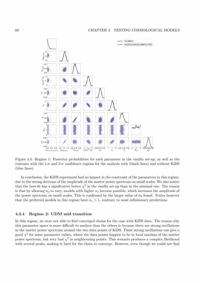
68 CHAPTER 4. TESTING COSMOLOGICAL MODELS
1.8
1.9
1.9
log β
udm
0.64
0.66
0.67
Ωλudm
3
3.1
3.1
ln10
10As
0.019
0.02
0.02
ωb
1
1
1.1
ns
0.64
0.65
0.65
h
-6
0
6
AIA
0.0530.0590.065
σ80.15 0.15 0.15atransitionudm
0.053
0.059
0.065
σ8
1.8 1.9 1.9logβudm
0.64 0.66 0.67Ωλudm
3 3.1 3.1ln1010As
0.019 0.02 0.02ωb
1 1 1.1ns
0.64 0.65 0.65
h-6 0 6
AIA
SLOW33
KiDSSLOW33COMPLETED
Figure 4.4: Regime 1: Posterior probabilities for each parameter in the vanilla set-up, as well as thecontours with the 1-σ and 2-σ confidence regions for the analysis with (black lines) and without KiDS(blue lines).
In conclusion, the KiDS experiment had no impact in the constraint of the parameters in this regime,due to the strong decrease of the amplitude of the matter power spectrum on small scales. We also noticethat the best-fit has a significative better χ2 in the vanilla set-up than in the minimal one. The reasonis that by allowing ns to vary, models with higher ns become possible, which increases the amplitude ofthe power spectrum on small scales. This is confirmed by the larger value of σ8 found. Notice howeverthat the preferred models in this regime have ns > 1, contrary to most inflationary predictions.
4.3.4 Regime 2: UDM mid transition
In this regime, we were not able to find converged chains for the case with KiDS data. The reason whythis parameter space is more difficult to analyse than the others is because there are strong oscillationsin the matter power spectrum around the two data points of KiDS. These strong oscillations can give agood χ2 for some parameter values, where the data points happen to be in local maxima of the matterpower spectrum, but very bad χ2 in neighbouring points. This scenario produces a complex likelihoodwith several peaks, making it hard for the chain to converge. However, even though we could not find

4.3. ANALYSIS 69
reliable statistical constraints, we were able to find particular models that match the observations aswell as ΛCDM, as we can see in Tables 4.8 and 4.10.
In Tables 4.7 and 4.8 we present the results for the second regime in the minimal set-up. We noticethat the best-fit is significantly better than in the first regime, and the amount of formed structure(as measured by σ8) is higher. In Fig. 4.5 we show the corresponding contours. The strong contrastbetween the smooth contours of the no-KiDS analysis and the plots from the non-converged chain iswell visible.
Parameters best-fit mean±σ 95% lower 95% upper
at 0.06362 0.06282+0.0024−0.0017 0.0581 0.06707
logβ,udm 3.092 3.1+0.048−0.056 2.989 3.214
ΩΛudm 0.6886 0.6885+0.00077−0.00078 0.687 0.6901
ln1010As 3.113 3.114+0.0041−0.0039 3.106 3.122
− lnLmin = 5386.33, minimum χ2 = 1.077e+ 04
Table 4.7: Estimated best-fit, mean, 1-σ uncertainty and the 2-σ intervals constraints for regime 2 inthe minimal set-up without KiDS data.
Parameters best-fit mean±σ 95% lower 95% upper
at 0.06472 0.06433+nannan nan nan
logβ,udm 3.036 3.05+nannan nan nan
ΩΛudm 0.6879 0.6884+nannan nan nan
ln1010As 3.11 3.111+nannan nan nan
AIA 2.603 1.727+nannan nan nan
σ8 0.302 0.3049+nannan nan nan
− lnLmin = 5432.23, minimum χ2 = 1.086e+ 04
Table 4.8: Estimated best-fit, mean, 1-σ uncertainty and the 2-σ intervals constraints for regime 2 inthe minimal set-up with KiDS data.

70 CHAPTER 4. TESTING COSMOLOGICAL MODELS
2.9
3.1
3.3
log β
udm
0.69
0.69
0.69
Ωλudm
3.1
3.1
3.1
ln10
10As
-3.3
0.41
4.1
AIA
0.27 0.3 0.33
σ80.055 0.061 0.068atransitionudm
0.27
0.3
0.33
σ8
2.9 3.1 3.3
logβudm0.69 0.69 0.69
Ωλudm
3.1 3.1 3.1ln1010As
-3.3 0.41 4.1AIA
FAST2
KiDSF2c
Figure 4.5: Regime 2: Posterior probabilities for each parameter in the minimal set-up, as well as thecontours with the 1-σ and 2-σ confidence regions for the analysis with (black lines) and without KiDS(blue lines).
Parameters best-fit mean±σ 95% lower 95% upper
at 0.0726 0.0687+0.00474−0.00398 0.0613 0.0768
logβ,udm 2.87 2.966+0.097−0.16 2.757 3.215
ΩΛudm 0.7105 0.7091+0.0058−0.0059 0.6977 0.7204
ln1010As 3.092 3.099+0.0087−0.014 3.081 3.12
ωb 0.0229 0.02265+0.00025−0.00034 0.02206 0.02327
ns 0.951 0.9578+0.0056−0.01 0.9436 0.9762
h 0.6953 0.6932+0.0046−0.005 0.6836 0.7029
− lnLmin = 5378.17, minimum χ2 = 1.076e+ 04
Table 4.9: Estimated best-fit, mean, 1-σ uncertainty and the 2-σ intervals constraints for regime 2 inthe vanilla set-up without KiDS data.

4.3. ANALYSIS 71
Parameters best-fit mean±σ 95% lower 95% upper
at 0.06718 0.06603+nannan nan nan
logβ,udm 3.024 3.021+nannan nan nan
ΩΛudm 0.7095 0.7077+nannan nan nan
ln1010As 3.102 3.106+nannan nan nan
ωb 0.02237 0.02248+nannan nan nan
ns 0.9592 0.9619+nannan nan nan
h 0.693 0.692+nannan nan nan
AIA −4.584 −4.103+nannan nan nan
σ8 0.3385 0.324+nannan nan nan
− lnLmin = 5396.25, minimum χ2 = 1.079e+ 04
Table 4.10: Estimated best-fit, mean, 1-σ uncertainty and the 2-σ intervals constraints for regime 2 inthe vanilla set-up with KiDS data.
2.6
3
3.3
log β
udm
0.69
0.71
0.72
Ωλudm
3.1
3.1
3.1
ln10
10As
0.022
0.023
0.024
ωb
0.94
0.96
0.99
ns
0.68
0.69
0.71
h
-6
-2.1
1.9
AIA
0.27 0.32 0.37
σ80.055 0.068 0.08atransitionudm
0.27
0.32
0.37
σ8
2.6 3 3.3logβudm
0.69 0.71 0.72Ωλudm
3.1 3.1 3.1ln1010As
0.0220.0230.024ωb
0.94 0.96 0.99ns
0.68 0.69 0.71
h-6 -2.1 1.9AIA
SLOW222
teste3
Figure 4.6: Regime 2: Posterior probabilities for each parameter in the vanilla set-up, as well as thecontours with the 1-σ and 2-σ confidence regions for the analysis with (black lines) and without KiDS(blue lines).

72 CHAPTER 4. TESTING COSMOLOGICAL MODELS
Tables 4.9, 4.10 and Fig. 4.6 show the results of the vanilla set-up analyses. They are consistentwith the minimal set-up, with no statistical results from the KiDS case. While the best-fit model nolonger has a slope ns > 1, indicating that this regime is more capable of forming structure than regime1.
4.3.5 Regime 3: UDM early transition
In Tables 4.11, 4.12 and Fig. 4.7 we show the results of our analyses in this regime for the minimalset-up, while Tabs. 4.13, 4.14 and Fig. 4.8 show the results for the vanilla set-up. We can see that inthis range of values for the cosmological parameters KiDS strongly constraint the values of at and β.
The results for the two set-ups are consistent and we can clearly see for the first time the interestin using the weak lensing data. In fact, for example in Figs. 4.7 and 4.8, we see a strong reduction inthe UDM parameters contours when adding the KiDS data. In particular, the at distribution withoutweak lensing data is bimodal with the strongest peak at lower values (Fig. 4.8), while the addition ofKiDS data enhances the second peak (Fig. 4.8) dramatically changing the result. Indeed, comparingthe at results from Tab. 4.13 to Tab. 4.14 we see a strong shift in the mean value. The same happensfor the β parameter where 1-σ decreases from 28% to 2% in the minimal case (Tabs. 4.11 and 4.12).The gain is smaller in the case of the UDM vanilla set-up, due to the correlations with the extra freeparameters.
The parameter σ8 has now for the first time values compatible with the known ΛCDM values [55].Since we are adding KiDS to the Planck combination of data, we have more data points and consistentlyobtain stronger constraints on σ8 in comparison with the contours obtained in [55].
We can then conclude that fast and early transition UDM models are compatible with structureformation on quasi-linear scales at low redshift.
Parameters best-fit mean±σ 95% lower 95% upper
at 0.01182 0.01616+0.0079−0.0119 0.00209 0.03052
logβ,udm 5.63 4.631+1.2771−1.3052 3.0458 5.6281
ΩΛudm 0.6884 0.6884+0.0008−0.00078 0.6868 0.69
ln1010As 3.121 3.121+0.0019−0.002 3.117 3.125
− lnLmin = 5379.71, minimum χ2 = 1.076e+ 04
Table 4.11: Estimated best-fit, mean, 1-σ uncertainty and the 2-σ intervals constraints for regime 3 inthe minimal set-up without KiDS data.

4.3. ANALYSIS 73
Parameters best-fit mean±σ 95% lower 95% upper
at 0.0349 0.03614+0.0016−0.0015 0.03312 0.0389
logβ,udm 5.639 5.568+0.13−0.04 5.378 5.7
ΩΛudm 0.6886 0.6883+0.00086−0.00075 0.6867 0.6899
ln1010As 3.121 3.122+0.002−0.0021 3.118 3.126
AIA −4.333 −4.413+0.2701−1.4360 −5.8489 −2.4071
σ8 0.7726 0.7703+0.03−0.047 0.6967 0.8559
− lnLmin = 5413.66, minimum χ2 = 1.083e+ 04
Table 4.12: Estimated best-fit, mean, 1-σ uncertainty and the 2-σ intervals constraints for regime 3 inthe minimal set-up with KiDS data.
3.1
4.4
5.7
log β
udm
0.69
0.69
0.69
Ωλudm
3.1
3.1
3.1
ln10
10As
-6
-3.4
-0.82
AIA
0.71 0.9 1.1
σ80.001 0.021 0.04atransitionudm
0.71
0.9
1.1
σ8
3.1 4.4 5.7
logβudm0.69 0.69 0.69
Ωλudm
3.1 3.1 3.1ln1010As
-6 -3.4 -0.82AIA
FAST1
KiDS11
Figure 4.7: Regime 3: Posterior probabilities for each parameter in the minimal set-up, as well as thecontours with the 1-σ and 2-σ confidence regions for the analysis with (black lines) and without KiDS(blue lines).
We can also look for correlations on the two-dimensional plots of Figs. 4.7 and 4.8. In comparisonwith the first regime we no longer have the correlation between ns and β, and we obtain values ofns very similar to the ones obtained for ΛCDM. We also lost the anti-correlation between ΩΛudm and

74 CHAPTER 4. TESTING COSMOLOGICAL MODELS
β. In fact we cannot conclude in this case if the correlation still exist, since the values of β are veryconstrained near the maximum value allowed and we cannot see if there is any correlation trend. Wealso do not see a correlation between β and σ8, however a correlation is expected since the value ofβ is strongly correlated with the Jeans scale that will affect the matter power spectrum at the scaleswhere σ8 is calculated. We observe that there is new a anti-correlation between As and ΩΛudm that didnot exist in the first regime. On the contrary, now at and σ8 seem to have a correlation that we wereunable to see in the first regime since at was always near its minimum value allowed. This correlationis expected since the value of at is also related to the Jean scale.
Finally, since our model is now sensitive to KiDS data, we get for the first time a measurementof the instrinsic alignment amplitude. In particular, we find a negative value in agreement with thevalues obtained in [55] for ΛCDM. We also find a correlation between the value of σ8 and the intrinsicalignment, because the intrinsic alignment affects the amplitude of the power spectrum at the measuredscales.The negative value of AIA indicates that the alignment is dominated by the cross term in Eq. 4.24 andnot by the auto-correlation term.
Parameters best-fit mean±σ 95% lower 95% upper
at 0.005355 0.01516+0.0025−0.014 0.00213 0.04128
logβ,udm 5.458 5.001+0.7−0.21 4.038 5.7
ΩΛudm 0.7088 0.709+0.0056−0.0053 0.6981 0.7198
ln1010As 3.12 3.119+0.0033−0.0042 3.111 3.128
ωb 0.02254 0.02249+0.00019−0.00019 0.0221 0.02289
ns 0.9734 0.9734+0.0037−0.0049 0.964 0.9836
h 0.6925 0.6924+0.0044−0.0043 0.6837 0.7011
− lnLmin = 5370.78, minimum χ2 = 1.074e+ 04
Table 4.13: Estimated best-fit, mean, 1-σ uncertainty and the 2-σ intervals constraints for regime 3 inthe vanilla set-up without KiDS data.
Parameters best-fit mean±σ 95% lower 95% upper
at 0.03723 0.03007+0.0120.003 0.03356 0.04144
logβ,udm 5.521 5.365+0.33−0.046 4.772 5.7
ΩΛudm 0.7084 0.7085+0.0053−0.0054 0.6978 0.719
ln1010As 3.122 3.121+0.0032−0.0048 3.114 3.131
ωb 0.02253 0.02252+0.00021−0.00019 0.02213 0.02291
ns 0.9752 0.9752+0.0043−0.0054 0.9655 0.9855
h 0.6919 0.6922+0.0042−0.0044 0.6834 0.7008
AIA −3.673 −3.085+0.3749−2.6643 −5.7489 5.7212
σ8 0.8336 0.8286+0.067−0.11 0.671 1.057
− lnLmin = 5406.97, minimum χ2 = 1.081e+ 04
Table 4.14: Estimated best-fit, mean, 1-σ uncertainty and the 2-σ intervals constraints for regime 3 inthe vanilla set-up with KiDS data.
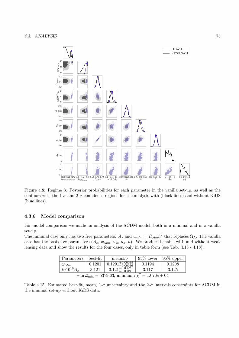
4.3. ANALYSIS 75
3.4
4.5
5.7
log β
udm
0.69
0.71
0.72
Ωλudm
3.1
3.1
3.1
ln10
10As
0.022
0.022
0.023
ωb
0.96
0.98
0.99
ns
0.68
0.69
0.7
h
-6
-3.5
-1
AIA
0.72 0.92 1.1
σ80.001 0.021 0.042atransitionudm
0.72
0.92
1.1
σ8
3.4 4.5 5.7logβudm
0.69 0.71 0.72Ωλudm
3.1 3.1 3.1ln1010As
0.0220.0220.023ωb
0.96 0.98 0.99ns
0.68 0.69 0.7
h-6 -3.5 -1AIA
SLOW11
KiDSSLOW11
Figure 4.8: Regime 3: Posterior probabilities for each parameter in the vanilla set-up, as well as thecontours with the 1-σ and 2-σ confidence regions for the analysis with (black lines) and without KiDS(blue lines).
4.3.6 Model comparison
For model comparison we made an analysis of the ΛCDM model, both in a minimal and in a vanillaset-up.The minimal case only has two free parameters: As and wcdm = Ωcdmh
2 that replaces ΩΛ. The vanillacase has the basis five parameters (As, wcdm, wb, ns, h). We produced chains with and without weaklensing data and show the results for the four cases, only in table form (see Tab. 4.15 - 4.18).
Parameters best-fit mean±σ 95% lower 95% upper
ωcdm 0.1201 0.1201+0.00038−0.00036 0.1194 0.1208
ln1010As 3.121 3.121+0.0022−0.0019 3.117 3.125
− lnLmin = 5379.63, minimum χ2 = 1.076e+ 04
Table 4.15: Estimated best-fit, mean, 1-σ uncertainty and the 2-σ intervals constraints for ΛCDM inthe minimal set-up without KiDS data.

76 CHAPTER 4. TESTING COSMOLOGICAL MODELS
Parameters best-fit mean±σ 95% lower 95% upper
ωcdm 0.1199 0.12+0.00032−0.00037 0.1193 0.1207
ln1010As 3.12 3.121+0.0018−0.002 3.117 3.124
AIA 0.7002 0.8844+0.3333−0.3114 0.3114 1.6214
σ8 0.8563 0.8564+0.0019−0.0022 0.8525 0.8606
− lnLmin = 5412.43, minimum χ2 = 1.082e+ 04
Table 4.16: Estimated best-fit, mean, 1-σ uncertainty and the 2-σ intervals constraints for ΛCDM inthe minimal set-up with KiDS data.
Parameters best-fit mean±σ 95% lower 95% upper
ωcdm 0.1169 0.1169+0.001−0.0011 0.1148 0.119
ln1010As 3.119 3.119+0.0033−0.0022 3.1128 3.1253
ωb 0.02249 0.02252+0.00019−0.00018 0.02215 0.02289
ns 0.973 0.9733+0.0037−0.0041 0.9656 0.9816
h 0.6926 0.6929+0.0044−0.0045 0.6841 0.7019
− lnLmin = 5370.54, minimum χ2 = 1.074e+ 04
Table 4.17: Estimated best-fit, mean, 1-σ uncertainty and the 2-σ intervals constraints for ΛCDM inthe vanilla set-up without KiDS data.
Parameters best-fit mean±σ 95% lower 95% upper
ωcdm 0.117 0.1168+0.001−0.0011 0.1146 0.119
ln1010As 3.119 3.119+0.0042−0.0041 3.11 3.127
ωb 0.02252 0.02251+0.00017−0.00021 0.02215 0.02294
ns 0.9737 0.9735+0.0044−0.0041 0.9649 0.982
h 0.6929 0.6934+0.0047−0.0045 0.6843 0.7026
AIA −0.9944 −0.8434+0.69−0.77 −2.239 0.6273
σ8 0.8475 0.8465+0.0041−0.0043 0.838 0.8552
− lnLmin = 5394.00, minimum χ2 = 1.079e+ 04
Table 4.18: Estimated best-fit, mean, 1-σ uncertainty and the 2-σ intervals constraints for ΛCDM inthe vanilla set-up with KiDS data.
We start by comparing the best-fit values for each case with ΛCDM (Tab. 4.19). We confirm thatregime 1, that we already ruled out, is very different from the ΛCDM values. The other cases, speciallyUDM3, have similar best-fit values for the standard models as ΛCDM.

4.3. ANALYSIS 77
Parameters ΛCDM UDM1 UDM2 UDM3(no KiDS/KiDS) (no KiDS/KiDS) (no KiDS/KiDS) (no KiDS/KiDS)
h 0.6926/0.6929 0.6439/0.6449 0.6953/0.6930 0.6925/0.695ln1010As 3.119/3.119 3.056/3.056 3.092/3.102 3.120/3.119ωb 0.02249/0.02252 0.0200/0.0201 0.02290/0.02237 0.02254/0.02246ns 0.973/0.9737 1.048/1.044 0.951/0.9592 0.9734/0.9749ΩΛudm / ΩΛ 0.7094/0.7094 0.6536/0.6557 0.7105/0.7095 0.7088/0.7123AIA −−/−0.9944 −−/−3.163 −−/−4.584 −−/−4.632χ2 5370.54/5394.00 5537.99/5600.97 5378.17/5396.25 5370.78/5407.85
Table 4.19: Best-fit values for ΛCDM and the three regimes of the UDM model, with and withoutKiDS.
We took the matter power spectrum of the best-fit UDM3 model obtained from the analysis withoutKiDS and computed its σ8 value. We found σ8 = 0.8218. Comparing with the result obtained from theanalysis with KiDS (σ8 = 0.8063) we expect a similar tension between the predicted values of σ8 fromPlanck and KiDS as in ΛCDM.
We also compute a number of information criteria to make a quantitative model comparison withΛCDM. These criteria are the Bayesian information criteria (BIC), defined as [70, 71]
BIC = −2 ln Lmax + klnN , (4.27)
the Deviance information criteria (DIC), following [72]
DIC = 2〈χ2〉 − χ2min , (4.28)
and the Akaike information criteria (AIC) [70]
AIC = 2k − 2 ln Lmax. (4.29)
These criteria depend on the best-fit χ2, mean χ2 over the sample, number of model parameters kand number of data points N . In general, a large number of model parameters penalises the model. Soa model with more parameters needs to have a better best-fit in order to be favoured in these compar-isons.Tables 4.20 - 4.22 show the values found for the three criteria, plus the best-fit χ2 and reduced χ2 forthe four models in the two set-ups and the two combinations of data.
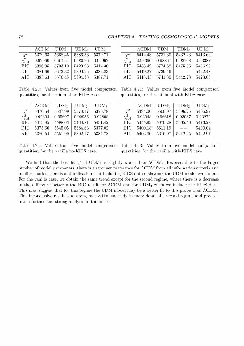
78 CHAPTER 4. TESTING COSMOLOGICAL MODELS
ΛCDM UDM1 UDM2 UDM3χ2 5379.63 5668.45 5386.33 5379.71χ2
red 0.92960 0.97951 0.93076 0.92962BIC 5396.95 5703.10 5420.98 5414.36DIC 5381.66 5673.32 5390.95 5382.83AIC 5383.63 5676.45 5394.33 5387.71
Table 4.20: Values from five model comparisonquantities, for the minimal no-KiDS case.
ΛCDM UDM1 UDM2 UDM3χ2 5412.43 5731.30 5432.23 5413.66χ2
red 0.93366 0.98867 0.93708 0.93387BIC 5438.42 5774.62 5475.55 5456.98DIC 5419.27 5739.46 −− 5422.48AIC 5418.43 5741.30 5442.23 5423.66
Table 4.21: Values from five model comparisonquantities, for the minimal with-KiDS case.
ΛCDM UDM1 UDM2 UDM3χ2 5370.54 5537.99 5378.17 5370.78χ2
red 0.92804 0.95697 0.92936 0.92808BIC 5413.85 5598.63 5438.81 5431.42DIC 5375.60 5545.05 5384.63 5377.02AIC 5380.54 5551.99 5392.17 5384.78
Table 4.22: Values from five model comparisonquantities, for the vanilla no-KiDS case.
ΛCDM UDM1 UDM2 UDM3χ2 5394.00 5600.97 5396.25 5406.97χ2
red 0.93048 0.96618 0.93087 0.93272BIC 5445.99 5670.28 5465.56 5476.28DIC 5400.18 5611.19 −− 5430.04AIC 5406.00 5616.97 5412.25 5422.97
Table 4.23: Values from five model comparisonquantities, for the vanilla with-KiDS case.
We find that the best-fit χ2 of UDM3 is slightly worse than ΛCDM. However, due to the largernumber of model parameters, there is a stronger preference for ΛCDM from all information criteria andin all scenarios there is and indication that including KiDS data disfavours the UDM model even more.For the vanilla case, we obtain the same trend except for the second regime, where there is a decreasein the difference between the BIC result for ΛCDM and for UDM2 when we include the KiDS data.This may suggest that for this regime the UDM model may be a better fit to this probe than ΛCDM.This inconclusive result is a strong motivation to study in more detail the second regime and proceedinto a further and strong analysis in the future.

Chapter 5
Conclusions
This dissertation allowed me to learn the full procedure of how to test a cosmological model. Startingfrom learning a new cosmological model allowed me to study the problems related to ΛCDM and GRand gain a broader view of several proposed solutions. Then studying the theoretical details of themodel gave me the opportunity to understand in more detail the evolution of scalar perturbations,how structure is formed and how it depends on a cosmological model. Then I was able to master aBoltzmann code (CLASS) which involved a review of the C programming language. Having modifiedthe code, I was in a position to solve the equations of perturbations for this specific model. For thefuture, this will be an important expertise that will give me the chance to work on new models and newobservables, such as solving the tensor modes of perturbation and extracting the gravitational wavespredicted from a cosmological model. This dissertation also allowed me to explore the world of param-eter estimation and gain expertise in an MCMC code, which makes a bridge between the theoreticalquantities obtained from CLASS and the observable data.Finally, I learnt many details about various cosmological data, using the likelihood codes of each dataset.
The analysis made in this dissertation leads to the conclusion that this UDM model is a viablecosmological model, compatible with the structure formation data used.As in all scientific analysis, we made several assumptions and verifications that are important to keepin mind.First of all, we verified that the large oscillations produced for some parameters values were real and nota numerical artefact. To verify this, we used a different numerical integrator and considered differentapproximations to the Heaviside function.The oscillations impede to properly compute a non-linear scale in the standard way. In addition thereis no non-linear prescription developed specifically for UDM models. For these reasons, we decided tokeep only the linear or quasi-linear data points from the weak lensing dataset. The points kept fromthe various cosmic shear power spectrum at various redshift bins probe the scale range k = [0.28, 0.82]of the matter power spectrum. By using these data points in two different ΛCDM analysis (with andwithout making the Halofit non-linear correction) we verified that the error in the likelihood is of order10 %.Another assumption, was to divide the n-dimension parameter space in three separate regimes, in orderto discard the volume where most of the models produced a sound speed larger than one and reachconvergence faster. This division granted us to study three specific cases of the model: one where thematter power spectrum strongly decreases at small scales, suppressing structure formation; a case where

80 CHAPTER 5. CONCLUSIONS
the scales that we used to test against KiDS are in a strong oscillatory regime, giving regions of thespace parameter with very good results next to regions of the space parameter with bad results; and athird case where the oscillations of the matter power spectrum only appears on very small scales andallow structure formation. In the first and third regime, due to the smoothness of the matter powerspectrum in the tested regions the chains were able to converge. In the second regime we were notable to made a complete analysis, but we were able to find UDM models with good agreement withthe observations. To obtain results for the second case we expect in the future to divide this spaceparameter in more parts or preferentially use a different sampling method that can better account formultiple likelihood peaks than the MCMC, such as the Nested Sampling.
We also performed the same analysis for ΛCDM without the HALOFIT non-linear corrections andfrom the comparison between our UDM model and ΛCDM we could conclude that our model is stilla strong candidate and a model capable of forming structure. However, a strong preference for theΛCDM model still remains.
There are several ways in which we could try to improve our analysis in future work. Besides theimprovement in the statistical analysis, in particular for the second case, we may also improve thetheoretical matter power spectrum by including the non-linear corrections. This will pass by being ableto implement the HALOFIT or other non-linear correction to our UDM model. This will be mandatoryto use if we want to test this model with the future data from the Euclid space mission.
We may also consider a different approach to the treatment of the UDM perturbations. In thisdissertation we always performed a standard procedure to deal with the linear perturbation and thenapply, when possible, non-linear corrections that start to appear at late times. However, in futureworks this method may also be revisited and we should check if a new approach for the case of modelswith large oscillations in the density contrast must be considered. This is because large oscillationscan produce, in some scale, a large amplitude in the density contrast giving rise to a non-linear regimemuch earlier in time. Then, the linear density contrast goes down again as it oscillates and the powerspectrum today is linear at that scale. However, we might consider that linear evolution is no longervalid from the time of the oscillation peak, and from this time onwards that scale could be removedfrom the linear evolution, and this effect could backreact on the evolution of the other scales.The oscillations are indeed caused by the variation of the sound speed. As a test, we fix the sound speedto zero in the perturbation module of CLASS and we were able to obtain a matter power spectrum withno oscillations. This give rises to possible ideas that allow the model to be well behaved and removethe large oscillations obtained. One option might be to construct a lagrangian for this model, where weobtain a more generalised fluid, or even just consider the fluid to be non-adiabatic. This will introducea new degree of freedom, related to the fact that the variation of pressure now has a dependency on theentropy, allowing us to fix the sound speed and reduce the oscillations. These new approaches usuallygive rise to new degrees of freedom that will penalise the model according to the information criteriaused in Sec. 4.6. However, it is important to consider all possible variations of a model that are realistand physically allowed. A model should not be ignored just because it requires more degrees of freedom.It could turn out to be the true description of the Universe.
Another possibility is to continue working with this model as it is, but considering the backreactioneffect discussed in Sec. 2.3. This backreaction was already implemented in CLASS for the GCG and

81
based on the results obtained for the GCG (see Appendix A) it might have a strong influence in thematter power spectrum of the UDM model.
Therefore, there are may aspects of the UDM models that may be refined and many variations thatare worth exploring, motivated by our results that these models are still viable given current structureformation data.

82 CHAPTER 5. CONCLUSIONS

Appendices


Appendix A
Results for the GCG
In this appendix, we show results from our implementation of the generalised Chaplygin gas (GCG),introduced in Section 2.2. The main goal of implementing this model was to compare our results withpublished ones.The comparison was successful, and we may now also discuss some of the models’ features.
In Figs. A.1 and A.2 we show the density contrast obtained when using the GCG for two differentscales. Just like in Fig. 3.30, there is a much smoother pattern in the oscillations compared with theUDM model with fast transition. These oscillations, as shown in Fig. A.3 also result in a matter powerspectrum with some oscillations.
We also considered the backreaction of the collapsed regions on the evolution of the linear den-sity contrast, as described in Section 2.3. The evolution of the two components, δ+ and δ− is shownin Fig. A.4, A.5, A.6 for three different scales, together with the evolution of δcdm in a flat ΛCDM model.
We see that δ+, the density contrast of the collapsed regions, grows as CDM while δ− behaves asin the standard GCG model. The presence of the collapsed regions smooths out the oscillations in thefinal matter power spectrum, as shown in Fig. A.7.This is a very interesting case and we have already implemented this approach for the UDM model forfuture analyses.

86 APPENDIX A. RESULTS FOR THE GCG
Figure A.1: Evolution of δGCG and δcdm over time for the intermediate scale k = 0.1, for Achap = 0.72and α = 0.2.
Figure A.2: Evolution of δGCG and δcdm over time for the small scale k = 10, for Achap = 0.72 andα = 0.2.

87
Figure A.3: Matter power spectrum for Achap = 0.72 and α = 0.2.
Figure A.4: Evolution of δ+,GCG, δ−,GCG and δcdm over time for the large scale k = 0.01, for Achap =0.72, α = 0.2 and using a backreaction parameter εi = 0.4.

88 APPENDIX A. RESULTS FOR THE GCG
Figure A.5: Evolution of δ+,GCG, δ−,GCG and δcdm over time for the intermediate scale k = 0.1, forAchap = 0.72, α = 0.2 and using a backreaction parameter εi = 0.4.

89
Figure A.6: Evolution of δ+,GCG, δ−,GCG and δcdm over time for the small scale k = 10, for Achap = 0.72,α = 0.2 and using a backreaction parameter εi = 0.4.
Figure A.7: Matter power spectrum for Achap = 0.72, α = 0.2 and using a backreaction parameterεi = 0.4.

90 APPENDIX A. RESULTS FOR THE GCG

Appendix B
Continuous approximations to theHeaviside function
In order to investigate that the large oscillations were not a numerical artifact, we decided to use dif-ferent continuous approximations to the Heaviside step function.We considered various popular S-shaped curves, also called sigmoid curves.
First attempt
H(a− at) = 12 [1 +×tanh (β (a− at))] . (B.1)
We started by considering the well-known logistic function.This attempt was unsuccessful since this approximation gives a negative speed of sound for a certainperiod of time, as seen in Fig. B.1.

92 APPENDIX B. CONTINUOUS APPROXIMATIONS TO THE HEAVISIDE FUNCTION
Figure B.1: Speed of sound for the first attempt, with at = 0.01, ΩΛudm = 0.7 and β = 500.
This result in a exponential growth of the density contrast for the fluid, and therefore, for the matterpower spectrum, shown in Fig. B.2. This results is of course not found in the observed universe.
Figure B.2: Matter power spectrum for the first attempt with at = 0.01, ΩΛudm = 0.7 and β = 500.

93
Second attempt
H(a− at) = 12
1 + β (a− at)(1 + β2 (a− at)2
)1/2
. (B.2)
In this attempt we obtained the same result as in the previous one, finding again a negative soundspeed, as shown in Fig. B.1.
Figure B.3: Speed of sound for the second attempt, with at = 0.01, ΩΛudm = 0.7 and β = 500.
Third attempt
H(a− at) = 12
[1 + β (a− at)
1 + β|a− at|
]. (B.3)
With this approximation we were not even able to compute any good result.
Fourth attempt
H(a− at) = 2πatan (exp (β (a− at))) . (B.4)
This function is similar to the one used in our UDM model. It only differs in having an exponentialin the argument of arctan. It turns out to be an interesting viable function that may deserve furtherconsideration in future works.Its main interesting feature is that it produces a sound speed that remains null after the peak the attransition (see Fig. B.4) This is not always the case for the original function, where the sound speedslowly increases from zero after the peak. This new feature allows for a very smooth matter spectrum,

94 APPENDIX B. CONTINUOUS APPROXIMATIONS TO THE HEAVISIDE FUNCTION
as shown in Fig. B.5, even though large oscillations are still formed for models with later transitions,as shown in Fig. B.6
Figure B.4: Speed of sound for the fourth attempt, with at = 0.01, ΩΛudm = 0.7 and β = 500.

95
Figure B.5: Matter power spectrum for the fourth attempt with at = 0.01, ΩΛudm = 0.7 and β = 500.
However, for higher values of at what could be a numerical problem remains:
Figure B.6: Matter power spectrum for the fourth attempt with at = 0.09, ΩΛudm = 0.7 and β = 500.

96 APPENDIX B. CONTINUOUS APPROXIMATIONS TO THE HEAVISIDE FUNCTION
Discussion
After testing these new functions it has become clearer that an approximation to the Heaviside functionis not only a mathematical device to connect the two regimes of the UDM model, but it contains a lotof physics in it. This is related to the fact that even if these functions have exactly the same shape, itsderivatives are not the same, resulting in different evolutions for the equation of state and the soundspeed. A different function consequently represents a new model, with different characteristics.We also found no evidences for numerical issues in our CLASS implementation.
Bibliography
[1] Amendola L., Tsujikawa S., Dark Energy (Book), Cambridge University Press (2010).
[2] Baumann D. Cosmology: Part III Mathematical Tripos (Lecture)
[3] Lifshitz E. M. Republication of: On the gravitational stability of the expanding universe, J. Phys.(USSR) 10 116 (1946)
[4] Carroll S. Spacetime and Geometry: An Introduction to General Relativity (Book), Pearson (2003).
[5] Bartelmann M. Cosmology (Lecture), Institut fur Theoretische Astrophysik Universitat Heidelberg.
[6] Planck Collaboration Planck 2015 results. XIII. Cosmological parameters, Astron.Astrophys. 594A13 (2016).
[7] Chung-Pei Ma, Bertschinger E. Cosmological Perturbation Theory in the Synchronous and Confor-mal Newtonian Gauges, Astrophys.J. 455 7-25 (1995).
[8] W. H. Press and Vishniac, E. T. Ap. J.,239, 1. (1980)
[9] Yoo J., Watanabe Y. Theoretical Models of Dark Energy, Int.J.Mod.Phys. D21 1230002 (2012).
[10] Supernova Search Team Collaboration, Riess A. G. et. al. Type Ia supernova discoveries at z >1 from the Hubble Space Telescope: Evidence for past deceleration and constraints on dark energyevolution, Astrophys.J. 607 665-687 (2004).
[11] SDSS Collaboration, Eisenstein D. J. et. al. Detection of the baryon acoustic peak in the large-scalecorrelation function of SDSS luminous red galaxies, Astrophys.J. 633 560-574 (2005).
[12] Wetterich C. Cosmology and the Fate of Dilatation Symmetry, Nucl.Phys. B302 668 (1988).
[13] Ratra B. and Peebles P. Cosmological Consequences of a Rolling Homogeneous Scalar Field,Phys.Rev. D37 3406 (1988).
[14] Caldwell R., Dave R. and Steinhardt P. J. Cosmological imprint of an energy component withgeneral equation of state, Phys.Rev.Lett. 80 1582-1585 (1998).
[15] Zlatev I., Wang L.M. and Steinhardt P. J., Quintessence, cosmic coincidence, and the cosmologicalconstant, Phys.Rev.Lett. 82 896-899 (1999).
[16] Caldwell R. and Linder E. V. The Limits of quintessence, Phys.Rev.Lett. 95 141301 (2005).

98 BIBLIOGRAPHY
[17] Armendariz-Picon C., Mukhanov V. F. and Steinhardt P. J. A Dynamical solution to the problemof a small cosmological constant and late time cosmic acceleration, Phys.Rev.Lett. 85 4438-4441(2000).
[18] Armendariz-Picon C., Mukhanov V. F. and Steinhardt P. J. Essentials of k-essence, Phys.Rev.D63 103510 (2001).
[19] Wetterich C. The Cosmon model for an asymptotically vanishing time dependent cosmological ’con-stant’, Astron.Astrophys. 301 321-328 (1995).
[20] Amendola L., Coupled quintessence, Phys.Rev. D62 043511 (2000).
[21] Capozziello S., Carloni S. and Troisi A. Quintessence without scalar fields, RecentRes.Dev.Astron.Astrophys. 1 625 (2003).
[22] Carroll S. M., Duvvuri V., Trodden M. and Turner M. S. Is cosmic speed - up due to new gravita-tional physics?, Phys.Rev. D70 043528 (2004).
[23] Nojiri S., Odintsov S., Unified cosmic history in modified gravity: From F(R) theory to Lorentznon-invariant models, D., Phys.Rept., 505,59 (2011).
[24] Dvali G., Gabadadze G. and Porrati M. 4-D gravity on a brane in 5-D Minkowski space, Phys.Lett.B485 208-214 (2000).
[25] Deffayet C. Cosmology on a brane in Minkowski bulk, Phys.Lett. B502 199-208 (2001).
[26] Tomita K. A local void and the accelerating universe, Mon.Not.Roy.Astron.Soc. 326 287 (2001).
[27] Alnes H., Amarzguioui M. and Gron O. An inhomogeneous alternative to dark energy?, Phys.Rev.D73 083519 (2006).
[28] Kamenshchik A. Y., Moschella U. and Pasquier V. An Alternative to quintessence, Phys.Lett. B511265-268 (2001).
[29] Bento M., Bertolami O. and SenA. Generalized Chaplygin gas, accelerated expansion and darkenergy matter unifcation, Phys.Rev. D66 043507 (2002).
[30] Sandvik H., Tegmark M., Zaldarriaga M. and Waga I. The end of unified dark matter?, Phys.Rev.D69 123524 (2004).
[31] Amendola L., Waga I. Observational constraints on silent quartessence, JCAP 0511 009 (2005).
[32] Kumar S., Sen A.A. Clustering GCG: a viable option for unified dark matter-dark energy?, JCAP10, 036 (2014).
[33] Avelino P.P., Bolejko K., Lewis G.F. Nonlinear Chaplygin Gas Cosmologies, Phys.Rev. D89 no.10,103004 (2014).
[34] Wang Y., Wands D., Xu L., De-Santiago J., Hojjati A. Cosmological constraints on a decomposedChaplygin gas, Phys. Rev. D 87, 083503 (2013).

BIBLIOGRAPHY 99
[35] Wands D., De-Santiago J., Wang Y. Inhomogeneous vacuum energy, Class. Quantum Grav.29,145017 (2012).
[36] De-Santiago J., Wands D., Wang Y. Inhomogeneous and interacting vacuum energy, Proceedingsof 4th International Meeting on Gravitation and Cosmology (MGC 4), p.183-196 (2014).
[37] Scherrer R. J. Purely kinetic k-essence as unified dark matter, Phys.Rev.Lett. 93 011301 (2004).
[38] Piattella O.F., Bertacca D. Gravitational potential evolution in Unified Dark Matter Scalar FieldCosmologies: an analytical approach, Mod.Phys.Lett. A26 2277-2286 (2011).
[39] Piattella O.F., Bertacca D., Bruni M., Pietrobon D. Unified Dark Matter models with fast transi-tion, JCAP 1001 014 (2010).
[40] Bertacca D., Bruni M., Piattella O.F., Pietrobon D. Unified Dark Matter scalar field models withfast transition, JCAP 1102 018 (2011).
[41] Bruni M., Lazkoz R. and Rozas-Fernandez A. Phenomenological models for Unified Dark Matterwith fast transition, Mon. Not. R. Astron. Soc.431,2907 (2013).
[42] Camera S., Kitching T. D., Heavens A. F., Bertacca D., Diaferio A. Measuring Unified Dark Matterwith 3D cosmic shear, Mon.Not.Roy.Astron.Soc. 415 399-409 (2011).
[43] Mukhanov V. Physical Foundations of Cosmology, (Book) Cambridge University Press (2005).
[44] Ferreira V., Unified Models of Dark Energy and Dark Matter (Master Dissertation), Universidadedo Porto (2014).
[45] Nadkarni-Ghosh S., Refregier A. The Einstein-Boltzmann equations revisited, Mon. Not. Roy. As-tron. Soc. 471 2391 (2017).
[46] Lesgourgues J. The Cosmic Linear Anisotropy Solving System (CLASS) I: Overview, CERN-PH-TH/2011-081, LAPTH-009/11 (2011).
[47] Seljak U., Zaldarriaga M. A Line of Sight Approach to Cosmic Microwave Background Anisotropies,Astrophys.J.469:437-444 (1996).
[48] Lewis A., Challinor A., Lasenby A. Efficient Computation of CMB anisotropies in closed FRWmodels, Astrophys.J.538:473-476 (2000).
[49] Doran M. CMBEASY:: an Object Oriented Code for the Cosmic Microwave Background, JCAP0510 011 (2005).
[50] Blas D., Lesgourgues J., Tram T. The Cosmic Linear Anisotropy Solving System (CLASS)II:Approximation schemes, arXiv:1104.2933 [astro-ph.CO] (2011).
[51] Lazkoz R., Leanizbarrutia I.,and Salzano V. Cosmological constrains on fast transition UnifiedDark Energy/Matter models , PRD93,043537 (2016).
[52] Bartelmann M., Schneider P. Weak gravitational lensing , Phys.Rept. 340 291-472 (2001).

100 BIBLIOGRAPHY
[53] The Virgo Consortium, Smith R.E., Peacock J.A., Jenkins A., White S.D.M., Frenk C.S., PearceF.R., Thomas P.A., Efstathiou G.,Couchmann H.M.P. Stable clustering, the halo model and nonlin-ear cosmological power spectra, Mon.Not.Roy.Astron.Soc.341:1311 (2003).
[54] Hildebrandt H., Viola M., Heymans C., Joudaki S., Kuijken K., Blake C., Erben T., Joachimi B.,Klaes D., Miller L. et al. KiDS-450: Cosmological parameter constraints from tomographic weakgravitational lensing, Mon.Not.Roy.Astron.Soc. 465 1454 (2017).
[55] Kohlinger F., Viola M., Joachimi B., Hoekstra H., Van Uitert E., Hildebrandt H., Choi A., ErbenT., Heymans C., Joudaki S. et al. KiDS-450: The tomographic weak lensing power spectrum andconstraints on cosmological parameters, arXiv:1706.02892 [astro-ph.CO] (2017).
[56] Audren B., Lesgourgues J., Benabed K., Prunet S. Conservative Constraints on Early Cosmology:an illustration of the Monte Python cosmological parameter inference code, JCAP 1302 001 (2013).
[57] Lewis A., Bridle S. Cosmological parameters from CMB and other data: A Monte Carlo approach,Phys.Rev. D66 103511 (2002).
[58] Feroz F., Hobson M.P. Multimodal nested sampling: an efficient and robust alternative to MCMCmethods for astronomical data analysis, Mon. Not. Roy. Astron. Soc., 384, 2, 449-463 (2008).
[59] Feroz F., Hobson M.P., Bridges M. MultiNest: an efficient and robust Bayesian inference tool forcosmology and particle physics, Mon. Not. Roy. Astron. Soc. 398: 1601-1614 (2009).
[60] Feroz F., Hobson M.P., Cameron E., Pettitt A.N. Importance Nested Sampling and the MultiNestAlgorithm, arXiv:1306.2144 [astro-ph.IM] (2013).
[61] Foreman-Mackey D., Hogg D. W., Lang D., Goodman J. emcee: The MCMC Hammer,arXiv:1202.3665 [astro-ph.IM] (2012).
[62] Akeret J., Seehars S., Amara A., Refregier A., Csillaghy A. CosmoHammer: Cosmological pa-rameter estimation with the MCMC Hammer, Astronomy and Computing, Volume 2, Pages 27-39,(2013).
[63] BOSS Collaboration The clustering of galaxies in the SDSS-III Baryon Oscillation Spectro-scopic Survey: baryon acoustic oscillations in the Data Releases 10 and 11 Galaxy samples,Mon.Not.Roy.Astron.Soc. 441 no.1, 24-62 (2014).
[64] BOSS Collaboration Quasar-Lyman α Forest Cross-Correlation from BOSS DR11: Baryon Acous-tic Oscillations, JCAP 1405 027 (2014).
[65] Ross A. J., Samushia L., Howlett C., Percival W. J., Burden A., Manera M. The cluster-ing of the SDSS DR7 main Galaxy sample - I. A 4 per cent distance measure at z = 0.15,Mon.Not.Roy.Astron.Soc. 449 no.1, 835-847 (2015).
[66] Beutler F., Blake C., Colless M., Jones D. H., Staveley-Smith L., Campbell L., Parker Q., SaundersW., Watson F. The 6dF Galaxy Survey: baryon acoustic oscillations and the local Hubble constant,Monthly Notices of the Royal Astronomical Society, Volume 416, Issue 4, pp. 3017-3032, (2011).
[67] SDSS Collaboration Improved cosmological constraints from a joint analysis of the SDSS-II andSNLS supernova samples, Astron.Astrophys. 568 A22 (2014)
BIBLIOGRAPHY 101
[68] Bennett C. L., Larson D., Weiland J. L., Jarosik N., Hinshaw G., Odegard N., Smith K. M.,Hill R. S., Gold B., Halpern M., Komatsu E., Nolta M. R., Page L., Spergel D. N., Wollack, E.,Dunkley J., Kogut A., Limon M., Meyer S. S., Tucker G. S., Wright E. L. Nine-year WilkinsonMicrowave Anisotropy Probe (WMAP) Observations: Final Maps and Results, The AstrophysicalJournal Supplement, Volume 208, Issue 2, article id. 20, 54 pp. (2013)
[69] Haslam C. G. T., Salter, C. J., Stoffel, H., Wilson, W. E. A 408 MHz all-sky continuum survey. II- The atlas of contour maps, Astronomy and Astrophysics Supplement Series, vol. 47, p. 1, 2, 4-51,53-142. (1982).
[70] Liddle A. How many cosmological parameters?, Mon.Not.Roy.Astron.Soc. 351 L49-L53 (2004).
[71] Kass R. E., Raftery A. E. Bayes Factors, J.Am.Statist.Assoc. 90 no.430, 773-795 (1995).
[72] Saez-Gomez D., Carvalho S. C., Lobo F. S. N., Tereno I. Constraining f(T, T) gravity models usingtype Ia supernovae, Phys. Rev. D 94, 024034 (2016).