1

Testing and modeling of a traditional timber mortise and

tenon joint

Artur O. Feio1 *, Paulo B. Lourenço2 & José S. Machado3

1,* Corresponding author. Auxiliar Professor, Faculty of Architecture, University Lusíada, Largo Tinoco de Sousa - 4760-108 Vila

Nova de Famalicão, Portugal. Phone: +351 252 309 200, fax: +351 252 376 363, email: arturfeio@gmail.com

2 Cathedratic Professor, Department of Civil Engineering, University of Minho, Azurém, P-4800-058 Guimarães, Portugal. Phone:

+351 253 510 209, fax: +351 253 510 217, email: pbl@civil.uminho.pt

3 Research Officer, National Laboratory for Civil Engineering, Timber Structures Division, Lisbon, Portugal. Phone: +351 21

8443299, fax: +351 21 8443025, email: saporiti@lnec.pt

Abstract: The structural safety and behaviour of traditional timber structures depends

significantly on the performance of their connections. The behaviour of a traditional

mortise and tenon timber joint is addressed using physical testing of full-scale

specimens. New chestnut wood and old chestnut wood obtained from structural

elements belonging to ancient buildings is used. In addition, the performance of

different semi and non-destructive techniques for assessing global strength is also

evaluated. For this purpose, ultrasonic testing, micro-drilling and surface penetration are

considered, and the possibility of their application is discussed based on the application

of simple linear regression models. Finally, nonlinear finite element analysis is used to

better understand the behaviour observed in the full-scale experiments, in terms of

failure mode and ultimate load.

The results show that the ultrasonic pulse velocity through the joint provides a

reasonable estimate for the effectiveness of the assembly between the rafter and brace

and novel linear regressions are proposed. The failure mechanism and load-

displacement diagrams observed in the experiments are well captured by the proposed

non-linear finite element analysis, and the parameters that affect mostly the ultimate

load of the timber joint are the compressive strength of wood perpendicular to the grain

2

and the normal stiffness of the interface elements representing the contact between

rafter and brace.

Keywords: Ancient timber structures; Chestnut wood; Semi and Non-destructive

methods; Pilodyn; Resistograph; Ultrasonic testing; Experimental testing; Finite

element analysis; Nonlinear mechanics.

3

1. Introduction

In the past, timber structural design was dominated by carpenter know-how, resulting

from tradition and empirical knowledge. Even if it was evident that some members were

subjected to tension and others to compression stresses, the observation of old timber

structures indicates often a complex structural understanding. Deterioration of timber

trusses led often to some sort of anarchy in ancient structures due to continuous changes

and repair works, mostly with additional stiffening or propping, resulting in

heterogeneity of the members, a multiplicity of connections and diversity of supports.

With respect to traditional wood-wood joints, rules-of-thumb dominated the technology

and the present knowledge is still rather limited, Schmidt et al. (1996), Schmidt and

Scholl (2000) and Palma and Cruz (2007). However, there has been a growing interest

in this field, Parisi and Piazza (2000), Sandberg et al. (2000), Eckelman and Haviarova

(2008) and Haviarova and Eckelman (2009).

In the present research program, a mortise and tenon joint, see Figure 1, was selected

because it is one of the most commonly used in ancient timber structures and a typical

example of an interlocking joint. Mortise and tenon joints connect two or more linear

components, forming usually an “L” or “T” type configuration. The key problem found

in these joints is the possible premature failure induced in the structure caused by large

displacements in the joint, Parisi and Piazza (2002) and Min et al. (2011).

The bearing capacity of mortise and tenon joints is a function of the angle of the

connection, and length of the toe and mortise depth, Aman et al. (2008), Judd et al.

(2012) and Likos et al. (2012). The lack of knowledge about this particular joint is

determinant in the assessment of the load carrying capacity of existing wooden

structures, Eckelman et al. (2007), Shanks and Walker (2009), Branco (2008) and

Branco et al. (2011). Here, the objective are to quantify the strength capacity of the joint

4

by physical testing of full-scale specimens, to validate the possible usage of semi and

non-destructive testing techniques to predict the joint properties and the joint

effectiveness and to validate the adequacy of an anisotropic failure criterion to represent

the behaviour of the joint by the comparison between experimental and numerical

results.

The adopted semi-destructive methods (SDT) and non-destructive methods (NDT) for

the joints are the Pilodyn, Resistograph and ultrasonic tests, respectively, which are

standard techniques for wood testing, Biechele et al. (2010) and Kasal and Tannert

(2010). For testing the joint effectiveness the ultrasonic test was used, Saporiti and

Palma (2011).

For the purpose of numerical analysis wood is often considered as an orthotropic or

transverse isotropic material with different properties in three mutually orthogonal

directions, axial, radial and tangential, Stehn and Börjes (2004) and Vilar et al. (2007).

Here, the finite element method is adopted to simulate the structural behaviour and

obtain a better understanding of the failure process observed in experimental tests.

Calculations are performed using a plane stress continuum model and the failure

criterion is based on multi-surface plasticity, comprising an anisotropic Rankine yield

criterion for tension, combined with an anisotropic Hill criterion for compression. The

full Newton-Raphson method, with stiffness matrix update in each iteration is used in

the analyses carried out in this work.

In the case of timber joints, two-dimensional approaches, e.g. Bouchair and Vergne

(1995), and three-dimensional approaches, e.g. Guan and Rodd (2000) and Moses and

Prion (2003), have been used in the past. Therefore, calculations are performed here

using a plane stress continuum model combined with different thicknesses and possible

slip provided by the addition of interface elements. Given the adoption of a 2D model

5

some parameters could not be taken fully into account, namely geometric imperfections

(joints and members), the contact friction between tenon and mortise and non-uniform

stress distribution inside the joint.

The plane stress model can capture different strengths and softening/hardening

characteristics in orthogonal directions, Chen et al (2003) and Sawata and Yasumura

(2003). Using the finite element model, the influence of compression perpendicular to

the grain and elastic stiffness on the response is addressed in detail.

2. Description of test specimens

Chestnut wood (Castanea sativa Mill.) is usually present in historical Portuguese

buildings and all the wood used in the test specimens came from the North of Portugal.

In order to assess the influence of service time in the response, two groups were

considered: New Chestnut Wood (NCW), obtained from recently sawn timber, and Old

Chestnut Wood (OCW), obtained from structural elements belonging to ancient

buildings (date and precise origin unknown) with unknown load history. The old logs

were obtained from rehabilitation works and were provided by a specialist contractor

claiming that the wood has been in service for over 100 years. All specimens were

prepared by the same carpenter, under similar moisture conditions and aiming at

including the fewest possible defects. An electronic device registered the air

temperature and relative humidity during the tests. The average values of temperature

and relative humidity were 24 ± 2 ºC and 52 ± 12%, respectively. The time elapsed

between the tests and withdrawal of the specimens from the climatic chamber (less than

24 h) did not affect the conditioning of the specimens.

Each specimen consists of two timber elements, with a cross section of 9250 mm,

connected by a mortise and tenon joint without any pegs, see Figure 1. Because of their

6

frequency in the preliminary roofs survey undertaken, the angle between the elements is

65º. Density tests were carried out in samples removed from the specimens’ ends.

Similar average values were found for NCW and OCW group, with an average of 593.6

kg/m3 for NCW and 568.8 kg/m3 for OCW (4% difference), indicating that the sample

is relatively homogenous on average. The coefficient of variation in each sample is

high: 25% (NCW) and 31% (OCW), see Feio (2006) for details.

3 Experimental program

The specimens were tested under compression in order to assess local compressive

failure and slipping of the joint, see Figure 2. One hydraulic jack was used to apply a

compression force aligned with the rafter, with a programmed loading cycle. The

system included a support plate with stiffeners, able to rotate and to ensure verticality of

the brace. The support plate included a toe so that the rafter did not slide. The brace was

kept in the original vertical alignment with a horizontal bar, connected to a load cell.

The jack had a maximum loading capacity of 300 kN and a maximum stroke of

200 mm.

The displacements were measured using linear variable differential transducers

(LVDTs), with an accuracy of ±0.025 mm and continuously recorded until failure. The

vertical and horizontal displacements in the specimens were measured by two pairs of

LVDTs placed on opposite faces of the specimens.

The loading procedure consisted of the application of two monotonic load stages, EN

26891 (1991): firstly, the load was applied up to 50% of the estimated maximum load

and was maintained for 30s. The load was then reduced to 10% of the estimated

maximum load and maintained for another 30s. This procedure was repeated once again

7

and, thereafter, the load was increased until ultimate load or until a maximum slip of

15 mm between the two timber elements was reached.

A constant rate of loading corresponding to about 20% of the estimate maximum load

per minute was used, leading to a total testing time of about 9 to 12 minutes. Each load-

displacement (vertical displacement of the brace) curve was reduced to a force-

displacement plot. The ultimate load of the joint ( int, joultF ) was defined as the

conventional value corresponding to a strain equal to a 2% offset in the usual

terminology (Nbr7190, 1997), as shown in Figure 3.

3.1 Ultimate force and failure patterns

Table 1 shows the results of the tests in terms of ultimate force. The scatter found is

moderate, with the ultimate force ranging between 121.6 kN up and 161.5 kN. Even if

the number of specimens is rather low, the average force in terms of groups NCW and

OCW exhibits only a marginal difference. Specimen J_7 was discarded in this table

because the ultimate load found (98.5 kN) was very low and controlled by a local

defect: a longitudinal crack in the rafter.

The main characteristic of the adopted joint is that the direction of the grain of the two

assembled pieces it is not coincident, forming an acute angle. The rafter was loaded in

the direction parallel to the grain, whereas the brace was loaded at an oblique angle

inducing large stresses perpendicular to the grain. Due to the anisotropic behaviour of

wood, wood stressed parallel to the grain presents the highest values of strength.

Therefore, the rafter, stressed in compression parallel to the grain, easily penetrates the

brace. The compressive damage in the brace occurred either localized at the toe or

distributed along the full contact length. Often, out-of-plane bulging of the rafter under

the contact length was observed. In some cases, compressive damage was accompanied

8

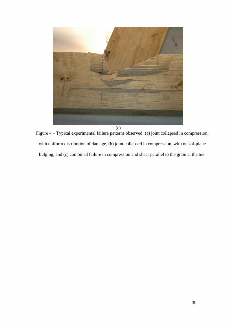
with shear failure in the rafter in front of the toe. Figure 4 illustrates the typical damages

observed at ultimate load.

The specimens were produced avoiding the presence of large defects although accepting

small defects. During the tests it was observed that the longitudinal and radial cracks of

moderate width (1-2 mm) in the rafter had a minor influence in the ultimate force and in

the global behaviour of the joints. The longitudinal pre-existing cracks tend to close and

the radial pre-existing cracks tend to open, being this behaviour more noticeable when

the cracks are close to the joint. On the other hand, the cracks present in the brace,

namely the longitudinal ones, show a tendency to propagate and to open during the

tests.

3.2 Load-displacement diagrams

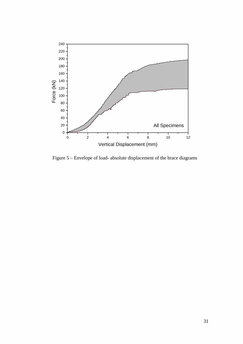
The envelope of all tests in terms of load-displacement diagrams, given by the vertical

force vs. vertical/absolute displacement of the brace, is given in Figure 5. In a first

phase, the diagrams exhibit a nonlinear response, which is due to the adjustment of the

tenon and the mortise. In a second phase, within working stress levels, the response

exhibits an approximately linear branch up to the ultimate force, which occurred at an

average displacement of 7.5 mm. It is noted that unloading-reloading cycles within

working stress levels provide a constant stiffness, which is higher than the loading

stiffness, see Figure 3. The justification of this behavior is attributed to the nonlinear

behavior of the interface between rafter and brace, which exhibits a closure

phenomenon. Finally, after the ultimate force the displacement increases rapidly with a

much lower stiffness, due essentially to the compressive failure of the wood in the rafter

around the joint.

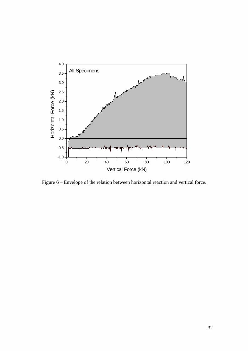
Figure 6 shows the relation between the vertical load and the horizontal load (reaction

load measured in the horizontal load cell). It can be observed that the horizontal reaction

9

varies between 0% and 3.5% of the vertical load. Such low values indicate that the

horizontal effects in the testing set-up can be neglected for practical purposes.

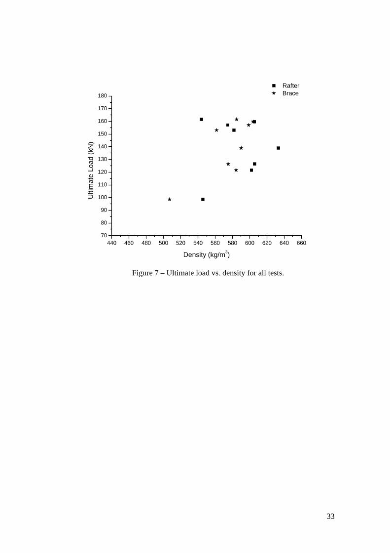
3.3 Correlations between density, ultimate load and stiffness

Higher wood density means usually higher stiffness and strength. Figure 7 shows the

relations between density and ultimate load, in case of the brace and of the rafter, as the

structural response is controlled by the rafter. It is clear that no correlation can be found.

A possible reason for this result is that the structural response is controlled by the local

characteristics of wood and density was measured at the specimens’ ends.

4. Semi and non-destructive testing

In order to investigate possible correlations and to validate the use of semi-destructive

and non-destructive techniques for the evaluation of the joint the Resistograph, the

Pilodyn and ultrasonic tests have been used, see Figure 8. Average values were

considered in all measurements, using two readings per specimen, per side, as described

below. A third reading was added only if the two first readings differed significantly.

Pilodyn and Resistograph have been carried out in samples removed from the elements

ends, in order not to affect the strength of the joint, whereas the ultrasonic tests were

carried out at the joint location.

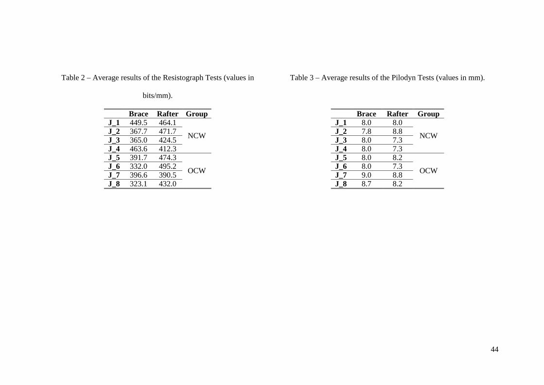
4.1. Resistograph and Pilodyn test procedure

Drilling and impact penetration was made on planes TL and LR, which, in real cases,

represents the accessible faces of timber elements. Micro-drilling measurements were

made using the Resistograph 3450-S and a 3 mm diameter drill bit. The resistographic

measure (RM) was calculated from the diagram obtained with the Resistograph, see

Lourenço et al. (2007), as the ratio between the integral of the area of the diagram and

the length l of the drilled perforation. The average results are presented in Table 2. The

10

Pilodyn 6J can measure the penetration of a metallic needle with 2.5 mm of diameter,

which is inversely proportional to the density of the wood, evaluating the surface

hardness or resistance to superficial penetration. The average results are presented in

Table 3.

4.2. Ultrasonic test procedure

A Pundit/Plus device (ultrasound generator) and a pair of cylinder-shaped transducers

(150 kHz) were used for ultrasonic testing. In all tests, performed after cutting the joints

but before load testing, coupling between the transducers and the specimens was

assured by a conventional hair gel, and a constant coupling pressure was applied on top

of the transducers by means of a rubber spring. Given the dimensions of the wood

elements and the diameter of the transducers used ( = 25 mm), a reference testing

mesh was defined on the central mid-third of each element, as shown in Figure 8. Five

distinct locations were defined, corresponding to three distinct zones of testing: (a) three

locations in the brace, (b) one location in the rafter, and (c) one location in the joint.

The tests in the brace and rafter aimed at characterizing the mechanical properties of the

elements in the zones nearby the joint. The test across the joint tried to evaluate in a

qualitative way the effectiveness of the assembly between the two elements. A through-

transmission indirect method (both transducers placed on the same surface) was adopted

measuring the wave propagation velocity parallel to the grain in each element and joint.

The average and the standard deviation results for the ultrasonic pulse velocity, for each

considered group, are presented in Table 4.

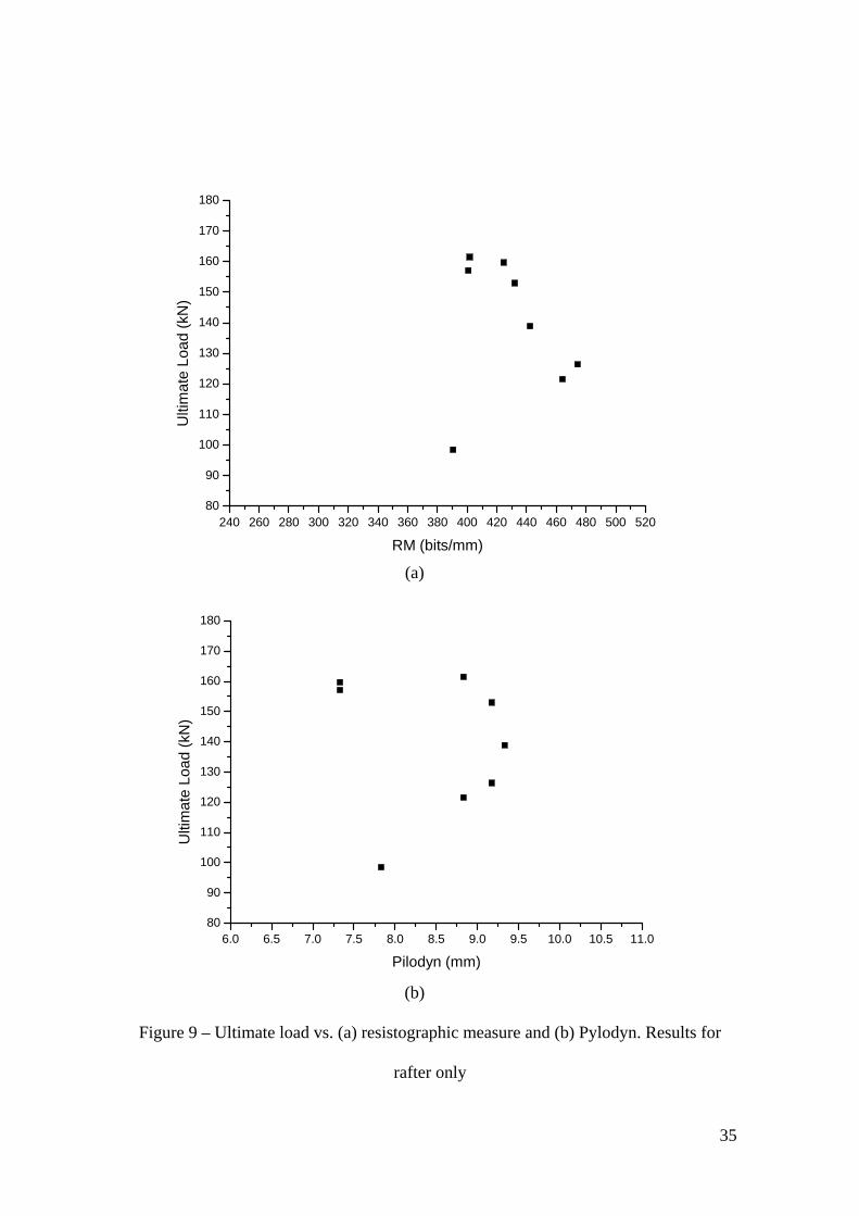
4.3. Results and correlations with semi and non-destructive tests

Figure 9 shows the correlations between the ultimate load and the measurements made

in the rafter using the Pilodyn and Resistograph techniques. Because the measurements

have been made in specimens’ ends and not at the joint location, no correlation could be

11

found. This conclusion holds if the rafter and brace are considered together, Feio

(2006). Similar results were found for the mechanical properties of chestnut

perpendicular to the grain in Lourenço et al. (2007).

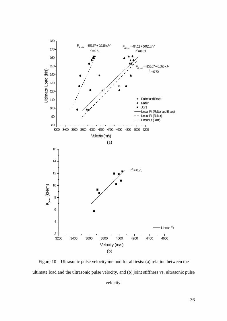
Figure 10a illustrates the relation between the ultimate load and the ultrasonic pulse

velocity. The results show that ultrasonic pulse velocity could be a good indicator for

the prediction of the ultimate load. Here, it is noted that the results using local

measurements only in the rafter, or rafter and brace together provide better correlations

than measurements across the joint. In the latter, also the stiffness of the joint is taken

into account, meaning that the ultrasonic pulse velocity is much lower. The joint

stiffness is also a relevant parameter for the estimation of deformations and strength of

existing timber structures. Figure 10b illustrates the correlation between joint stiffness

intjok and the ultrasonic pulse velocity across the joint. A clear linear correlation was

found, indicating that it seems possible to estimate joint stiffness from ultrasonic

testing.

5. Numerical simulation

In order to further discuss the experimental results, a finite element simulation of the

tests has been carried out and continuum quadratic elements (8-noded) were used to

represent the wood and to represent the line interface between rafter and brace quadratic

elements (6-noded) were used. The integration schemes used are 22 Gauss

integration points for the continuum elements and 3 Lobatto integration points for the

interface elements. The simulations have been carried out using a globally convergent

solution process, combining a Newton-Raphson method with arc-length and line search.

The adopted failure criterion for wood consists of an extension of conventional

formulations for isotropic quasi-brittle materials to describe orthotropic behaviour. It is

12

based on multi-surface plasticity, including a Hill yield criterion for compression and a

Rankine yield criterion for tension, and having different strengths in the directions

parallel and perpendicular to the grain, see Lourenço et al. (1997) for details.

In the present case, the tensile part of the yield criterion was ignored due to the

irrelevant contribution of the tensile strength in the global behaviour of the joint. This

means that the yield surface reduces to the standard Hill criterion in compression. The

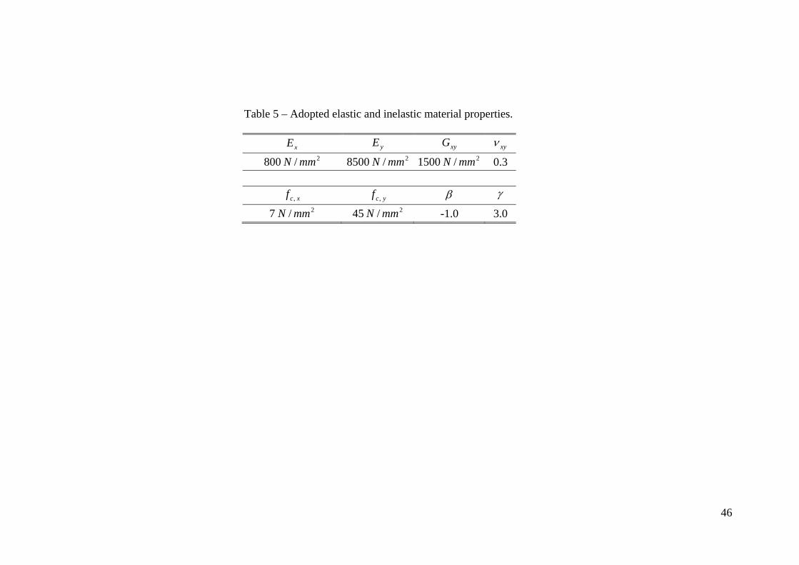
adopted elastic and inelastic materials properties are detailed in Table 5 and have been

obtained from a testing program aiming at characterizing chestnut, see Lourenço et al.

(2007) and Feio (2006).

Figure 11 illustrates the shape of the adopted yield criterion in the compression-

compression regime, which features an extreme degree of anisotropy with a ratio

156.0/ ,, ycxc ff .

5.1 Numerical vs. experimental results

A structured mesh is used for the rafter and the brace, whereas an irregular transition

mesh is used in the vicinity of the connection between rafter and brace. Interface

elements are also used between the rafter and the brace. The thickness ranges from

62 mm to 93 mm, as shown in Figure 12a. This aims at representing the thickness of the

mortise.

The comparison between numerical and experimental load-displacement diagrams is

given in Figure 12b. A preliminary analysis with an infinite stiffness of the interface,

assuming a fully rigid connection, indicated that such an assumption provided far too

stiff results. Therefore, the stiffness of the interface elements was obtained by inverse

fitting. Given this procedure and taking into account the possibility of using this model

towards other joint geometries and/or loadings, the model present a great sensitivity to

13

the stiffness of the interface elements. Thus, a first conclusion is that the stiffness of the

interface elements has considerable influence on the yield strength of timber joints.

In Figure 12b, three distinct situations are presented:

a numerical simulation with infinite stiffness of the interface elements in the normal

direction, kn, and shear direction, ks (9

infinite 10 sn kkk N/mm³);

a numerical simulation with an adjusted stiffness of the interface elements obtained

by inverse fitting of the experimental results ( fitk ), assuming that the shear and

normal stiffness are related via the Poisson’s coefficient by )1/(2/ vkk ns :

6000nk N/mm³ and 2308sk N/mm³;

a numerical simulation with a spring ( 610springk N/m) located in the brace to

simulate the reaction cell used in the experimental sets. The stiffness of the spring

was again obtained by inverse fitting of the experimental results, keeping the

adjusted stiffness of the interface elements.

For the purpose of numerical analysis, the load-displacement diagrams were corrected

with an offset that eliminates the upward curve related to the nonlinear behaviour of the

joint previous to full contact (joint closure). The numerical results, in terms of force-

displacement diagrams, with the adjusted stiffness for the interface elements, provide

very good agreement with the experimental results both in the linear and nonlinear

parts. The influence of the experimental horizontal restraint, simulated by a linear

spring, is only marginal.

A more relevant conclusion is that the usage of infinite stiffness for the interface (rigid

joint) results in an increase of the slope of the first part of the response, from 30 kN/mm

to 80 kN/mm (+ 266.7%). The ultimate force of the joint, given by an offset of the

14

linear stretch by 2% in terms of strain values, also changes from 130 kN to 152 kN (+

17%), once the joint becomes fully rigid.

Figure 13 shows the contour of minimum principal stresses at ultimate load. It is

possible to observe a concentration of stresses in a narrower band with peak stresses at

the joint (zone where the interface elements were placed), upon increasing loading. As

observed in the experiments, failure is governed by wood crushing, being the

compressive strength of the wood, in the direction perpendicular to the joint, exhausted

at failure.

5.2 Sensitivity study

A strong benefit of using numerical simulations is that parametric studies can be easily

carried out and the sensitivity of the response to the material parameters can be easily

evaluated. This allows a better understanding of the structural response. However, it is

important to understand the limitations of the model given the adoption of a 2D model,

as referred some parameters could not be taken fully into account, and the introduction

of interface elements referred. In this perspective a future 3D model can bring some

additional accuracy to the results now obtained.

The influence of the key parameters of the model in the response will be analyzed

separately. The values nk (normal stiffness of the interface), sk (tangent stiffness of the

interface), xE and yE (Young’s moduli in the directions parallel and perpendicular to

the grain, respectively) are assumed to be less well known and variations of 50% and

100% are made. xf and yf (compressive strengths in the directions parallel and

perpendicular to the grain, respectively) are assumed to be well known and variations of

+25% and -25% are made, corresponding to 0.75 and 1.25 times the initial value.

5.2.1 Normal and tangential stiffness of the interface

15

Figure 14a shows a comparison between the results of the variation of the normal joint

stiffness: with a reduction of 50% in nk , the ultimate force of the joint, given by an

offset of the linear stretch by 2%, decreases from 127.2 kN to 120 kN (-6%).

Multiplying nk by a factor of two the ultimate force of the joint, given by an offset of

the linear stretch by 2%, increases from 127.2 kN to 135.0 kN (+7%).

The reduction/increase of the normal stiffness of the interface also affects the global

stiffness of the joint; the global stiffness of the joint decreases as the normal stiffness of

the interface decreases, being more sensitive to this variation when compared with the

ultimate force. The reduction of 50% of the nk parameter, results in a decrease of the

slope of the first part of the response, from 32 kN/mm to 26 kN/mm (-23%). On the

other hand, the multiplication by a factor of 2 of this parameter results in an increase of

the slope of the first part of the response, from 32 kN/mm to 41 kN/mm (+ 28%).

Figure 14b shows a comparison between the results of the variation of the sk parameter.

The ultimate force is insensitive to a sk variation, whereas the reduction/increase of the

sk parameter affects the global stiffness of the joint: the global stiffness of the joint

decreases as the sk parameter decreases. The reduction of 50% of the sk parameter,

results in a decrease of the slope of the first part of the response, from 32 kN/mm to

28 kN/mm (-14%). On the other hand, the multiplication by a factor of 2 of this

parameter results in an increase of the slope of the first part of the response, from

32 kN/mm to 37 kN/mm (+16%).

5.2.2 Elastic modulus

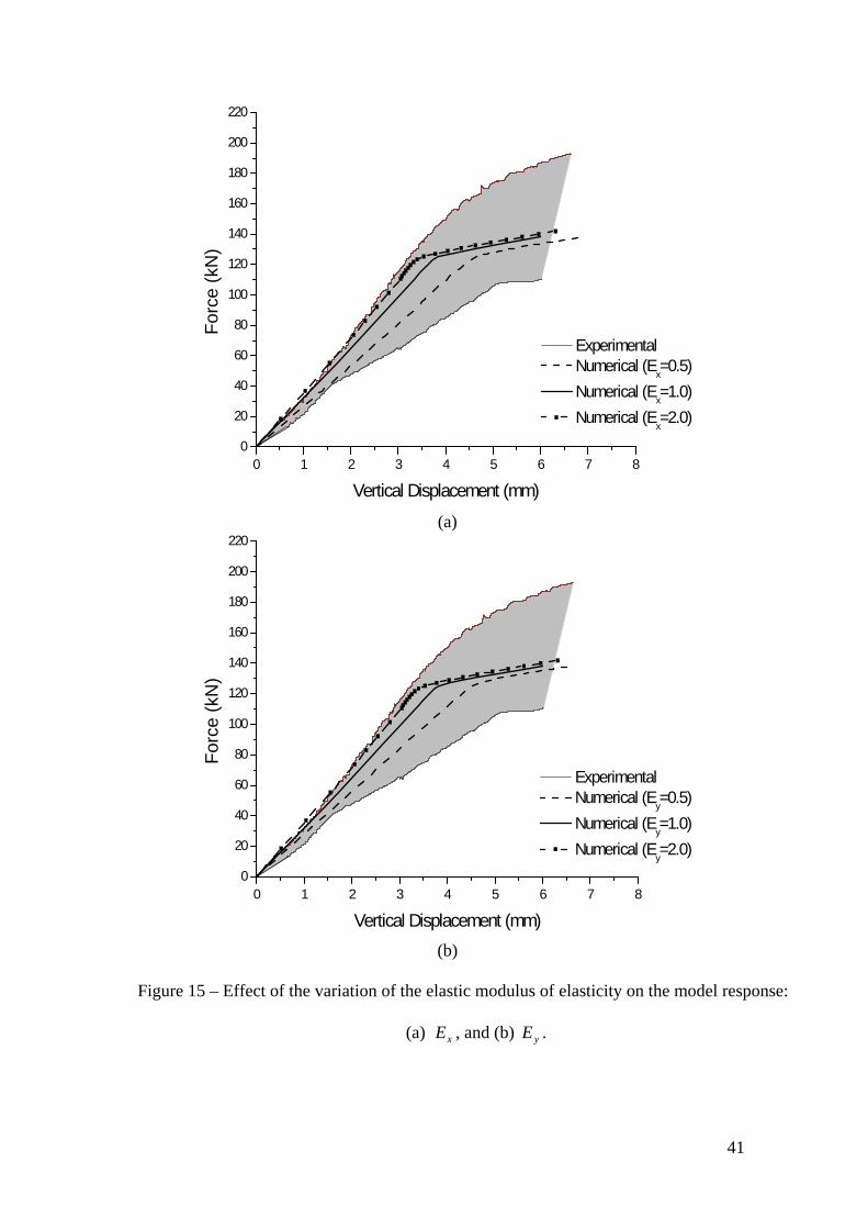
The effect of the variation of the modulus of elasticity parallel and perpendicular to the

grain was considered individually, see Feio (2006) for details. Figure 15 indicates that

the ultimate force is almost insensitive to the variation of the elastic modulus for wood

16

(± 4%), in both considered directions. The inclusion of the effects of the elastic modulus

does change significantly the elastic stiffness of the joint. The reduction of 50% of the

xE parameter, see Figure 15a, results in a decrease of the slope of the first part of the

response, from 32 kN/mm to 28 kN/mm (-14%). On the other hand, the multiplication

by a factor of 2 of this parameter results in an increase of the slope of the first part of the

response, from 32 kN/mm to 36 kN/mm (+13%).

The reduction of 50% of the yE parameter, see Figure 15b, results in a decrease of the

slope of the first part of the response, from 32 kN/mm to 28 kN/mm (-14%). On the

other hand, the multiplication by a factor of 2 of this parameter results in an increase of

the slope of the first part of the response, from 32 kN/mm to 36 kN/mm (+13%).

5.2.3 Compressive strength

Finally, the relationship between the global behaviour of the joint and the compressive

strength of wood in both considered directions is shown in Figure 16. It is apparent in

Figure 16a that the ultimate force and the global stiffness of the joint are insensitive to

the variation of the compressive strength of wood in the direction parallel to the grain.

Figure 16b indicates higher sensitivity of the ultimate force of the joint to the variation

of the compressive strength of wood in direction perpendicular to the grain, as expected:

with a reduction of 0,75, the ultimate force of the joint, given by an offset of the linear

stretch by 2‰, decreases from 130 kN to 100 kN (-30%); multiplying by a factor of

1.25 the ultimate force of the joint, given by an offset of the linear stretch by 2‰,

increases from 130 kN to 160 kN (+23%). However, the global stiffness of the joint is

insensitive to the variation of the compressive strength perpendicular to the grain.

6. Conclusions

17

Despite the wide use of mortise and tenon joints in existing timber structures scarce

information is available for design and in situ assessment. The objective of the present

study was to quantify the strength capacity of a wood-wood mortise and tenon joint by

physical testing of full-scale specimens. In addition, the performance of different semi

and non-destructive tests for assessing global joint strength was also evaluated. Finally,

the adequacy of an anisotropic failure criterion to represents the behaviour of a

traditional mortise and tenon joint was assessed from the comparison between

experimental and numerical results.

Two different wood groups have been used, one from new logs and another one from

old logs. Reducing the defects to a minimum, no influence could be attributed to service

time. Thus, safety assessment of new timber structures, made from old or new wood

elements, can be made using similar mechanical data.

Density, Resistograph and Pilodyn are recommended for qualitative assessment of

timber elements. On the contrary, ultrasonic testing provided reasonable correlations for

the joint strength. The results also show that the ultrasonic pulse velocity through the

joint provides a reasonable estimate for the joint stiffness, or effectiveness of the

assembly between the rafter and brace. Additionally, novel linear regressions have been

proposed for chestnut mortise and tenon joints with interlocking.

The failure mechanism and load-displacement diagrams observed in the experiments are

well captured by the used non-linear finite element analysis. Nevertheless, the normal

stiffness of the interface has considerable influence in the yield strength and

deformation of timber joints. The parameters that affect mostly the ultimate load of the

timber joint are the compressive strength of wood perpendicular to the grain and the

normal stiffness of the interface elements representing the contact between rafter and

brace. The tangential stiffness of the interface and the Young’s moduli of wood have

18

only very limited influence in the response. The compressive strength of wood parallel

to the grain has no influence in the response.

The sensitivity of ultimate force and stiffness of the joint towards the compression

perpendicular to the grain and the modulus of elasticity, respectively, shows that SDT

and NDT methods can provide some in situ information about the structural behavior of

traditional timber mortise and tenon joints. This statement is based on: the correlation

between ultrasonic velocity and ultimate load and stiffness found in the present study;

and, the correlations found between the dynamic modulus of elasticity (ultrasonic) and

the modulus of elasticity perpendicular to the grain determined by Lourenço et al

(2007). This information can be used to sustain a reliability analysis following the work

performed for other types of timber joints (Leijten et al 2004).

The correlation found between ultrasonic tests and joint performance can be important

and represent a step towards design/diagnosis, structural analysis and possible remedial

measures of chestnut timber structures. Also, in the design of new timber structures and

rehabilitation projects this correlation can be useful. However, without further

experimental investigations, namely in others timber joint types, this correlation should

be used as a comparative term, namely of the effectiveness of the joint, when analyzed

in terms of a specific structure. Future research should therefore concentrate on the

confirmation of this finding.

References

1. Aman, R., West, H., Cormier, D. (2008), An evaluation of loose tenon joint

strength. Forest Products Journal, 58(3), pp. 61-64.

19

2. Biechele, T., Chui, Y., Gong, M. (2010), Assessing stiffness on finger-jointed

timber with different non-destructive testing techniques. Proceedings of the

Final Conference of COST Action E53.

3. Bouchoir, A., Vergne, A. (1995), An application of the Tsai criterion as a

plastic-flow law for timber bolted joint modeling, Wood Science and

Technology, 30(1), p. 3-19

4. Branco, J. (2008), Influence of the joints stiffness in the monotonic and cyclic

behaviour of traditional timber trusses. Assessment of the efficacy of different

strengthening techniques. PhD thesis, University of Minho and University of

Trento.

5. Branco, J., Piazza, M., Cruz, P. J. S. (2011), Experimental evaluation of

different strengthening techniques of traditional timber connections.

Engineering Structures, Volume 33, Issue 8, Pages 2259–2270.

6. CEN (1991), EN 26891 – Timber structures. Joints made with mechanical

fasteners general principles for the determination of strength and deformation

characteristics. European Committee for Standardization, Brussels, Belgium.

7. CEN (2003), EN 408 – Timber structures. Structural timber and glued

laminated timber. Determination of some physical and mechanical properties.

European Committee for Standardization, Brussels, Belgium.

8. Chen, C., Lee, T., Jeng, D. (2003), Finite element modeling for the mechanical

behavior of dowel-type timber joints. Computers & Structures, 81(30–31), pp.

2731–2738

9. Eckelman, C., Akcay, H., Haviarova, E. (2007), Exploratory study of truss

heel joints constructed with round mortise and tenon joints. Forest Products

Journal, 57(9), pp. 68-72.

10. Eckelman, C., Haviarova, E. (2008), Rectangular mortise and tenon semirigid

joint connection factors. Forest Products Journal, 58(12), pp. 49-55.

11. Feio, A. (2006), Inspection and diagnosis of historical timber structures: NDT

correlations and structural behaviour, PhD Thesis, University of Minho,

Portugal. Available from www.civil.uminho.pt/masonry.

20

12. Guan, Z.W., Rodd, P.D. (2000), A three-dimensional finite element model for

locally reinforced timber joints made with hollow dowel fasteners, Canadian,

J. Civil Engineering, 27(4), p. 785-797

13. Haviarova, E., Eckelman, C. (2009), Semi-rigid connection factors for small

round mortise and tenon joints. Forest Products Journal. 59(9), pp. 55-60.

14. Judd, J., Fonseca, F., Walker, C., Thorley, P. (2012), Tensile strength of

varied-angle mortise and tenon connections in timber frames. Journal of

Structural Engineering, Vol. 137, No. 5, May 2012, pp. 636-644.

15. Kasal, B., Tannert, T. (2010), In situ Assessment of Structural Timber. Eds.

RILEM State of the Art Reports.

16. Leijten, A., Köhler, J., Jorissen, A. (2004), Review of probability data for

timber connections with dowel-type fasteners. Proceedings of the 37th

Meeting, International Council for Research and Innovation in Building and

Construction, Working Commission W18 – Timber Structures, CIB-W18,

Paper No. 37-7-13, Edinburgh, UK.

17. Likos, E., Haviarova, E., Eckelman, C., Erdil, Y., Ozcifci, A. (2012), Effect of

tenon geometry, grain orientation, and shoulder on bending moment capacity

and moment rotation characteristics of mortise and tenon joints. Wood and

Fiber Science, 44(4), pp. 1-8.

18. Lourenço, P., De Borst, R., Rots, J. (1997), A plane stress softening plasticity

model for orthotropic materials, Int. J. Numerical Methods in Engineering, 40,

p. 4033-4057.

19. Lourenço, P.B., Feio, A.O., Machado, J.S. (2007), Chestnut wood in

compression perpendicular to the grain: non-destructive correlations for test

results in new and old wood. Construction and Building Materials, Volume 21,

Issue 8, pp. 1617-1627.

20. Min, K., Na, Y., Qun, C. (2011), Studies on static performance of mortise and

tenon joint in traditional column and tie construction timber structure.

International Conference on Electric Technology and Civil Engineering

(ICETCE), pp. 6197 - 6200.

21

21. Moses, D., Prion, H. (2003), A three-dimensional model for bolted

connections in wood. Canadian Journal of Civil Engineering, 30(3), pp. 555–

567.

22. Palma, P., Cruz, H. (2007), Mechanical behaviour of traditional timber

carpentry joints in service conditions - results of monotonic tests. In From

material to Structure – Mechanical behaviour and failures of the timber

structures XVI International Symposium, Venice, Italy. ICOMOS IWC.

23. Parisi, M., Piazza, M. (2000), Mechanics of plain and retrofitted traditional

timber connections. Journal of Structural Engineering, 126(12):1395–1403.

24. Parisi, M., Piazza, M. (2002), Seismic behavior and retrofitting of joints in

traditional timber roof structures. Soil Dynamics and Earthquake Engineering,

Vol. 22, Issues 9–12, pp. 1183–1191.

25. Ross, R., Brashaw, B., Pellerin, R. (1998), Nondestructive evaluation of wood,

Forest Products Journal, 48(1), pp. 101-105.

26. Sandberg L.B., Bulleit, W.M., Reid, E.H. (2000), Strength and stiffness of oak

pegs in traditional timber-frame joints, J. Structural Engineering, ASCE,

126(6), p. 717-723.

27. Saporiti, J., Palma, P. (2011), Non-destructive evaluation of the bending

behaviour of in-service pine timber structural elements. Materials and

Structures, Vol. 44, 5, pp. 901-910.

28. Sawata K; Yasumura M (2003). Estimation of yield and ultimate strengths of

bolted timber joints by nonlinear analysis and yield theory. Journal of Wood

Science, 49(5), pp. 83–391.

29. Schmidt, R. J., MacKay, R. B., Leu, B. L. (1996), Design of joints in

traditional timber frame buildings, Proceedings of the International Wood

Engineering Conference, Vol. 4, pp. 240-247, New Orleans, LA. 28-31.

Reprinted in --, Timber Frame Joinery and Design Workbook, Timber Framers

Guild of North America, pp. 77-91.

30. Schmidt, R., Scholl, G. (2000), Load duration and seasoning effects on mortise

and tenon connections. Research Report, University of Wyoming, Department

of Civil and Architectural Engineering, Wyoming, pp. 111.

22

31. Shanks, J., Walker, P. (2009), Strength and stiffness of all-timber pegged

connections. Journal of Materials in Civil Engineering, 21(1), pp. 10–18.

32. Stehn, L., Borjes, K. (2004), The influence of nail ductility on the load

capacity of a glulam truss structure. Engineering Structures, 26(6), pp. 809–

816.

33. Villar, J. R., Guaita, M., Vidal, P., Arriaga, F. (2007), Analysis of the stress

state at the cogging joint in timber structures. Biosystems Engineering, Vol.

96, Issue 1, pp. 79–90.

23

List of Figures

Figure 1 – Details of a typical tenon and mortise joint, with the geometry adopted in the

testing program (dimensions in mm). 

Figure 2 – Aspects of the test set-up and location of LVDTs 

Figure 3 – Definition of the ultimate load from the force-displacement diagram. 

Figure 4 – Typical experimental failure patterns observed: (a) joint collapsed in

compression, with uniform distribution of damage, (b) joint collapsed in

compression, with out-of-plane bulging, and (c) combined failure in compression

and shear parallel to the grain at the toe. 

Figure 5 – Envelope of load- absolute displacement of the brace diagrams 

Figure 6 – Envelope of the relation between horizontal reaction and vertical force. 

Figure 7 – Ultimate load vs. density for all tests. 

Figure 8 – Location of semi-destructive and non-destructive tests. 

Figure 9 – Ultimate load vs. (a) resistographic measure and (b) Pylodyn. Results for

rafter only 

Figure 10 – Ultrasonic pulse velocity method for all tests: (a) relation between the

ultimate load and the ultrasonic pulse velocity, and (b) joint stiffness vs. ultrasonic

pulse velocity. 

Figure 11 – Shape of the proposed yield criterion for chestnut wood. Material

parameters: 0.7, xcf N/mm²; 45, ycf N/mm²; 0.1 ; 0.3 . 

Figure 12 – (a) localization of the interface elements, and (b) comparison between

numerical and experimental load-displacement diagrams. 

Figure 13 – Minimum principal stresses (values in N/m²) at ultimate load. 

Figure 14 – Effect of the variation of parameter: (a) nk , and (b) sk on the model

response. 

24

Figure 15 – Effect of the variation of the elastic modulus of elasticity on the model

response: 

Figure 16 – Effect of the variation of the compressive strength on the model response:

(a) xcf , , and (b) ycf , . 

25

List of Tables

Table 1 – Test results: ultimate force.

Table 2 – Average results of the Resistograph Tests (values in bits/mm).

Table 3 – Average results of the Pilodyn Tests (values in mm).

Table 4 – Results of the Ultrasonic Tests (average and standard deviation values in m/s).

Table 5 – Adopted elastic and inelastic material properties.

26

Figure 1 – Details of a typical tenon and mortise joint, with the geometry adopted in the

testing program (dimensions in mm).

27

Figure 2 – Aspects of the test set-up and location of LVDTs

28

0 1 2 3 4 5 6 7 8 9 10 11 12 130

2

4

6

8

10

12

14

16

Offset - 2%

ult, joint = 2%

For

ce (

N)

Displacement (mm)

Fult, joint

Figure 3 – Definition of the ultimate load from the force-displacement diagram.

29

(a)

(b)

30

(c)

Figure 4 – Typical experimental failure patterns observed: (a) joint collapsed in compression,

with uniform distribution of damage, (b) joint collapsed in compression, with out-of-plane

bulging, and (c) combined failure in compression and shear parallel to the grain at the toe.

31

0 2 4 6 8 10 120

20

40

60

80

100

120

140

160

180

200

220

240

All Specimens

For

ce (

kN)

Vertical Displacement (mm)

Figure 5 – Envelope of load- absolute displacement of the brace diagrams

32

0 20 40 60 80 100 120-1.0

-0.5

0.0

0.5

1.0

1.5

2.0

2.5

3.0

3.5

4.0

All Specimens

Hor

izon

tal F

orce

(kN

)

Vertical Force (kN)

Figure 6 – Envelope of the relation between horizontal reaction and vertical force.

33

440 460 480 500 520 540 560 580 600 620 640 66070

80

90

100

110

120

130

140

150

160

170

180

Rafter Brace

Ulti

ma

te L

oad

(kN

)

Density (kg/m3)

Figure 7 – Ultimate load vs. density for all tests.

34

Figure 8 – Location of semi-destructive and non-destructive tests.

35

240 260 280 300 320 340 360 380 400 420 440 460 480 500 52080

90

100

110

120

130

140

150

160

170

180U

ltim

ate

Lo

ad

(kN

)

RM (bits/mm)

(a)

6.0 6.5 7.0 7.5 8.0 8.5 9.0 9.5 10.0 10.5 11.080

90

100

110

120

130

140

150

160

170

180

Ulti

ma

te L

oad

(kN

)

Pilodyn (mm)

(b)

Figure 9 – Ultimate load vs. (a) resistographic measure and (b) Pylodyn. Results for

rafter only

36

3200 3400 3600 3800 4000 4200 4400 4600 4800 5000 520080

90

100

110

120

130

140

150

160

170

180

Rafter and Brace Rafter Joint Linear Fit (Rafter and Brace) Linear Fit (Rafter) Linear Fit (Joint)

Fult, joint

= -116.67 + 0.055 x V

Ulti

mat

e L

oad

(kN

)

Velocity (m/s)

r2 = 0.70

r2 = 0.68F

ult, joint = -94.13 + 0.051 x VF

ult, joint = -306.57 + 0.115 x V

r2 = 0.61

(a)

3200 3400 3600 3800 4000 4200 4400 46002

4

6

8

10

12

14

16

Linear Fit

Kjo

int (

kN/m

)

Velocity (m/s)

r2 = 0.75

(b)

Figure 10 – Ultrasonic pulse velocity method for all tests: (a) relation between the

ultimate load and the ultrasonic pulse velocity, and (b) joint stiffness vs. ultrasonic pulse

velocity.

37

Figure 11 – Shape of the proposed yield criterion for chestnut wood. Material parameters:

0.7, xcf N/mm²; 45, ycf N/mm²; 0.1 ; 0.3 .

38

(a)

0 1 2 3 4 5 6 7 80

20

40

60

80

100

120

140

160

180

200

220

KSpring, fit

Numerical Experimental

Kfit

For

ce (

kN)

Vertical Displacement (mm)

Kinfinite

(b) Figure 12 – (a) localization of the interface elements, and (b) comparison between numerical

and experimental load-displacement diagrams.

39

Figure 13 – Minimum principal stresses (values in N/m²) at ultimate load.

40

0 1 2 3 4 5 6 7 80

20

40

60

80

100

120

140

160

180

200

220

Experimental Numerical (k

n=0.5)

Numerical (kn=1.0)

Numerical (kn=2.0)

For

ce (

kN)

Vertical Displacement (mm)

(a)

0 1 2 3 4 5 6 7 80

20

40

60

80

100

120

140

160

180

200

220

Experimental Numerical (k

s=0.5)

Numerical (ks=1.0)

Numerical (ks=2.0)

For

ce (

kN)

Vertical Displacement (mm)

(b)

Figure 14 – Effect of the variation of parameter: (a) nk , and (b) sk on the model response.

41

0 1 2 3 4 5 6 7 80

20

40

60

80

100

120

140

160

180

200

220

Experimental Numerical (E

x=0.5)

Numerical (Ex=1.0)

Numerical (Ex=2.0)

For

ce (

kN)

Vertical Displacement (mm)

(a)

0 1 2 3 4 5 6 7 80

20

40

60

80

100

120

140

160

180

200

220

Experimental Numerical (E

y=0.5)

Numerical (Ey=1.0)

Numerical (Ey=2.0)

For

ce (

kN)

Vertical Displacement (mm)

(b)

Figure 15 – Effect of the variation of the elastic modulus of elasticity on the model response:

(a) xE , and (b) yE .

42

0 1 2 3 4 5 6 7 80

20

40

60

80

100

120

140

160

180

200

220

Experimental Numerical (f

c,x=0.75)

Numerical (fc,x

=1.0)

Numerical (fc,x

=1.25)

For

ce (

kN)

Vertical Displacement (mm)

(a)

0 1 2 3 4 5 6 7 80

20

40

60

80

100

120

140

160

180

200

220

Experimental Numerical (f

c,y=0.75)

Numerical (fc,y

=1.0)

Numerical (fc,y

=1.25)

For

ce (

kN)

Vertical Displacement (mm)

(b)

Figure 16 – Effect of the variation of the compressive strength on the model response:

(a) xcf , , and (b) ycf , .

43

Table 1 – Test results: ultimate force.

Ultimate Force (kN) Average Std. Dev. Group J_1 121.6

145.4 18.9 NCW J_2 161.5 J_3 159.7 J_4 138.9 J_5 126.4

145.5 16.7 OCW J_6 157.1 J_8 153.0

44

Table 2 – Average results of the Resistograph Tests (values in

bits/mm).

Table 3 – Average results of the Pilodyn Tests (values in mm).

Brace Rafter GroupJ_1 449.5 464.1

NCW J_2 367.7 471.7J_3 365.0 424.5J_4 463.6 412.3J_5 391.7 474.3

OCW J_6 332.0 495.2J_7 396.6 390.5J_8 323.1 432.0

Brace Rafter GroupJ_1 8.0 8.0

NCW J_2 7.8 8.8J_3 8.0 7.3J_4 8.0 7.3J_5 8.0 8.2

OCW J_6 8.0 7.3J_7 9.0 8.8J_8 8.7 8.2

45

Table 4 – Results of the Ultrasonic Tests (average and standard deviation values in m/s).

NCW

Brace Joint Rafter

Average 4484.0 3940.8 4776.0

Std. Dev. 182.2 34.0 131.1

OCW

Brace Joint Rafter

Average 4559.4 3826.3 4613.5

Std. Dev. 153.7 49.8 97.2

46

Table 5 – Adopted elastic and inelastic material properties.

xE yE xyG xy

2/800 mmN 2/8500 mmN 2/1500 mmN 0.3

xcf , ycf , 2/7 mmN 2/45 mmN -1.0 3.0