SoC Level Formal Verification - Test and Verification Solutions
Upload
hoangkhanhCategory
view
243download
2
Helical3D Validation Manual
Advanced Numerical SolutionsHilliard OH
February 24, 2005

ii

Contents
Preface xiii
1 Introduction 1
2 Calculation of contact pressure for a spur gear model using Calyx 32.1 Contact pressure for spur gear model with no tooth tip modifications . . . . . . . 3
2.1.1 The example file . . . . . . . . . . . . . . . . . . . . . . . . . . . . . . . . 32.1.2 Obtaining the contact pressure from the postprocessing menu . . . . . . . 82.1.3 Contact pressure from theoretical calculations . . . . . . . . . . . . . . . . 11
2.2 Contact pressure for spur gear model with linear tooth tip modification . . . . . 182.2.1 The example file . . . . . . . . . . . . . . . . . . . . . . . . . . . . . . . . 182.2.2 Obtaining the contact pressure from the postprocessing menu . . . . . . . 192.2.3 Obtaining contact pressure from theoretical calculations . . . . . . . . . . 22
2.3 Contact pressure for spur gear model with quadratic tooth tip modification . . . 332.3.1 The example file . . . . . . . . . . . . . . . . . . . . . . . . . . . . . . . . 332.3.2 Obtaining the contact pressure from the postprocessing menu . . . . . . . 332.3.3 Contact pressure from theoretical calculations . . . . . . . . . . . . . . . . 37
2.4 Contact pressure for spur gear model with lead crown tooth modification . . . . 452.4.1 The example file . . . . . . . . . . . . . . . . . . . . . . . . . . . . . . . . 452.4.2 Obtaining the contact pressure from the postprocessing menu . . . . . . . 472.4.3 Contact pressure from theoretical calculations . . . . . . . . . . . . . . . . 50
2.5 Conclusion . . . . . . . . . . . . . . . . . . . . . . . . . . . . . . . . . . . . . . . 55
3 Sub-surface stresses in a spur gear model using Calyx 573.1 The spur gear model with no tooth modification . . . . . . . . . . . . . . . . . . 57
3.1.1 The example file . . . . . . . . . . . . . . . . . . . . . . . . . . . . . . . . 573.1.2 Obtaining the sub-surface stress from the postprocessing menu . . . . . . 57
4 Calculation of transmission error for a spur and helical gear model usingCalyx 634.1 Introduction . . . . . . . . . . . . . . . . . . . . . . . . . . . . . . . . . . . . . . . 634.2 Measuring the transmission error using calyx . . . . . . . . . . . . . . . . . . . . 64
4.2.1 Comparison of transmission error values obtained from Calyx and LDPfor Spur gears . . . . . . . . . . . . . . . . . . . . . . . . . . . . . . . . . . 64
4.2.2 Comparison of transmission error values obtained from Calyx and LDPfor Helical gears . . . . . . . . . . . . . . . . . . . . . . . . . . . . . . . . 71
4.3 Conclusion . . . . . . . . . . . . . . . . . . . . . . . . . . . . . . . . . . . . . . . 71
5 Internal helical gear pair example 755.1 The example file . . . . . . . . . . . . . . . . . . . . . . . . . . . . . . . . . . . . 755.2 Results . . . . . . . . . . . . . . . . . . . . . . . . . . . . . . . . . . . . . . . . . . 81

iv CONTENTS
6 Internal helical gear with webbed rim 836.1 The example file . . . . . . . . . . . . . . . . . . . . . . . . . . . . . . . . . . . . 836.2 Modeling the rim . . . . . . . . . . . . . . . . . . . . . . . . . . . . . . . . . . . . 836.3 Results . . . . . . . . . . . . . . . . . . . . . . . . . . . . . . . . . . . . . . . . . . 85
7 Modeling splines using the Helical 3D program 877.1 Internal splines on external gear . . . . . . . . . . . . . . . . . . . . . . . . . . . 87
7.1.1 The example file . . . . . . . . . . . . . . . . . . . . . . . . . . . . . . . . 877.1.2 Modeling the splines . . . . . . . . . . . . . . . . . . . . . . . . . . . . . . 877.1.3 Results . . . . . . . . . . . . . . . . . . . . . . . . . . . . . . . . . . . . . 87
7.2 External splines on external gear . . . . . . . . . . . . . . . . . . . . . . . . . . . 917.2.1 The example file . . . . . . . . . . . . . . . . . . . . . . . . . . . . . . . . 917.2.2 Modeling the splines . . . . . . . . . . . . . . . . . . . . . . . . . . . . . . 917.2.3 Results . . . . . . . . . . . . . . . . . . . . . . . . . . . . . . . . . . . . . 93
7.3 External splines on internal gear . . . . . . . . . . . . . . . . . . . . . . . . . . . 957.3.1 The example file . . . . . . . . . . . . . . . . . . . . . . . . . . . . . . . . 957.3.2 Modeling the splines . . . . . . . . . . . . . . . . . . . . . . . . . . . . . . 957.3.3 Results . . . . . . . . . . . . . . . . . . . . . . . . . . . . . . . . . . . . . 97
7.4 Internal splines on internal gear . . . . . . . . . . . . . . . . . . . . . . . . . . . . 997.4.1 The example file . . . . . . . . . . . . . . . . . . . . . . . . . . . . . . . . 997.4.2 Modeling the splines . . . . . . . . . . . . . . . . . . . . . . . . . . . . . . 997.4.3 Results . . . . . . . . . . . . . . . . . . . . . . . . . . . . . . . . . . . . . 101
8 Example of topographic modification 1038.1 The example file . . . . . . . . . . . . . . . . . . . . . . . . . . . . . . . . . . . . 1038.2 Applying topographic modifications on the pinion tooth . . . . . . . . . . . . . . 1038.3 Results . . . . . . . . . . . . . . . . . . . . . . . . . . . . . . . . . . . . . . . . . . 107
9 Convergence study 1139.1 Effect of Tip radius on the max ppl normal stress . . . . . . . . . . . . . . . . . . 113
9.1.1 The example file . . . . . . . . . . . . . . . . . . . . . . . . . . . . . . . . 1139.1.2 Results and discussion . . . . . . . . . . . . . . . . . . . . . . . . . . . . . 118
9.2 Effect of Tooth thickness on the max ppl normal stress . . . . . . . . . . . . . . . 1219.3 Effect of number of elements in the face direction on the max ppl normal stress . 1239.4 Effect of displacement order on the max ppl normal stress . . . . . . . . . . . . . 1259.5 Conclusions . . . . . . . . . . . . . . . . . . . . . . . . . . . . . . . . . . . . . . . 125
10 Fatigue theory and life prediction using the Helical gear program 12710.1 Introduction . . . . . . . . . . . . . . . . . . . . . . . . . . . . . . . . . . . . . . . 12710.2 Fatigue characteristics . . . . . . . . . . . . . . . . . . . . . . . . . . . . . . . . . 12710.3 Low and High cycle fatigue . . . . . . . . . . . . . . . . . . . . . . . . . . . . . . 12810.4 Fatigue loading . . . . . . . . . . . . . . . . . . . . . . . . . . . . . . . . . . . . . 12810.5 Example of a laboratory fatigue testing . . . . . . . . . . . . . . . . . . . . . . . 13310.6 Gear fatigue failure . . . . . . . . . . . . . . . . . . . . . . . . . . . . . . . . . . . 13410.7 Running the Helical3D program for fatigue failure . . . . . . . . . . . . . . . . . 135
10.7.1 The example file . . . . . . . . . . . . . . . . . . . . . . . . . . . . . . . . 13510.7.2 Locating the point of maximum stress . . . . . . . . . . . . . . . . . . . . 13510.7.3 Results . . . . . . . . . . . . . . . . . . . . . . . . . . . . . . . . . . . . . 141
10.8 Calculating the fatigue life . . . . . . . . . . . . . . . . . . . . . . . . . . . . . . . 14210.8.1 Goodman’s Linear relationship . . . . . . . . . . . . . . . . . . . . . . . . 14310.8.2 Gerber’s parabolic relationship . . . . . . . . . . . . . . . . . . . . . . . . 14410.8.3 Soderberg’s linear relationship . . . . . . . . . . . . . . . . . . . . . . . . 144
CONTENTS v
10.8.4 Elliptic relationship . . . . . . . . . . . . . . . . . . . . . . . . . . . . . . 14410.9 Effect of rigid internal diameter on fatigue life . . . . . . . . . . . . . . . . . . . . 146
10.9.1 Locating the point of maximum stress . . . . . . . . . . . . . . . . . . . . 14610.9.2 Results . . . . . . . . . . . . . . . . . . . . . . . . . . . . . . . . . . . . . 150
10.10Fatigue life for a thin flexible rim model . . . . . . . . . . . . . . . . . . . . . . . 15010.10.1Locating the point of maximum stress . . . . . . . . . . . . . . . . . . . . 15010.10.2Results . . . . . . . . . . . . . . . . . . . . . . . . . . . . . . . . . . . . . 154
10.11Cumulative damage . . . . . . . . . . . . . . . . . . . . . . . . . . . . . . . . . . 15410.11.1Linear damage theory . . . . . . . . . . . . . . . . . . . . . . . . . . . . . 15410.11.2Gatts Cumulative damage theory . . . . . . . . . . . . . . . . . . . . . . . 156
10.12Fatigue life based on duty cycle for a gear set . . . . . . . . . . . . . . . . . . . 15710.13Calculating life based on cumulative damage theory . . . . . . . . . . . . . . . . 16310.14Conclusions . . . . . . . . . . . . . . . . . . . . . . . . . . . . . . . . . . . . . . . 163
A Values of m and n for various values of θ 165

vi CONTENTS

List of Figures
2.1 Graph of contact pressure against time for pinion tooth no.1 . . . . . . . . . . . 92.2 Grid pressure histogram for pinion tooth no.1 at t=0 (Contact Pressure = 1.596110E+005
at Time = 0.000000E+000. Range of contact pressure is from 0.000000E+000 to1.596110E+005 and each division corresponds to 2.000000E+004) . . . . . . . . . 10
2.3 Drawing defining the radius of curvature(R) and the roll angle(θ) . . . . . . . . . 122.4 Plot of tooth load against time for pinion tooth no.1 . . . . . . . . . . . . . . . . 132.5 Toothload histogram at t=0.0 . . . . . . . . . . . . . . . . . . . . . . . . . . . . . 142.6 A graph comparing Calyx’s and Hertz’s contact pressure predictions . . . . . . . 162.7 Linear tip relief applied to the pinion tooth . . . . . . . . . . . . . . . . . . . . . 182.8 Linear tip relief applied to the gear tooth . . . . . . . . . . . . . . . . . . . . . . 192.9 Graph of contact pressure against time for pinion tooth no.1 . . . . . . . . . . . 202.10 Grid pressure histogram for pinion tooth no.1 at t=0.5s (Contact Pressure at
Time = 5.000000E-001s. Range of contact pressure is from 0.000000E+000 to1.183206E+005 and each division corresponds to 2.000000E+004 . . . . . . . . . 21
2.11 Toothload histogram at t=0.5s . . . . . . . . . . . . . . . . . . . . . . . . . . . . 282.12 A graph comparing Calyx’s and Hertz’s contact pressure predictions for linear
modification at the teeth . . . . . . . . . . . . . . . . . . . . . . . . . . . . . . . . 302.13 A plot of contact pressure against time obtained from Calyx in the time range
from 0.0s to 0.2s . . . . . . . . . . . . . . . . . . . . . . . . . . . . . . . . . . . . 312.14 Quadratic tip relief applied to the pinion tooth . . . . . . . . . . . . . . . . . . . 332.15 Quadratic tip relief applied to the gear tooth . . . . . . . . . . . . . . . . . . . . 342.16 Plot of contact pressure against time for pinion tooth no.1 . . . . . . . . . . . . . 352.17 Grid pressure histogram for pinion tooth no.1 at t=0.5s (Contact Pressure at
Time= 5.000000E-001 is 1.241488E+005s. Range of contact pressure is from0.000000E+000 to 1.241488E+005 and each division corresponds to 2.000000E+004 36
2.18 Toothload histogram at t=0.5s . . . . . . . . . . . . . . . . . . . . . . . . . . . . 412.19 A graph comparing Calyx’s and Hertz’s contact pressure predictions for quadratic
modification at the teeth . . . . . . . . . . . . . . . . . . . . . . . . . . . . . . . . 432.20 Crowning applied to the pinion tooth . . . . . . . . . . . . . . . . . . . . . . . . . 452.21 Crowning applied to the gear tooth . . . . . . . . . . . . . . . . . . . . . . . . . . 462.22 Plot of contact pressure against time for pinion tooth no.1 . . . . . . . . . . . . . 482.23 Grid pressure histogram for crowned pinion tooth no.1 at t=0 (Contact Pressure at
Time= 0.00 is 2.014838E+005. Range of contact pressure is from 0.000000E+000to 2.014838E+005 and each division corresponds to 1.000000E+005 . . . . . . . . 49
2.24 Figure showing the crowning curvature . . . . . . . . . . . . . . . . . . . . . . . . 502.25 Toothload histogram at the t=0 . . . . . . . . . . . . . . . . . . . . . . . . . . . . 54
3.1 Graph of sub-surface Von Mises stress as a function of depth at pinion tooth no.1.The contact is at the pitch point. . . . . . . . . . . . . . . . . . . . . . . . . . . . 59

viii LIST OF FIGURES
3.2 Graph of sub-surface max. shear stress as a function of depth at pinion toothno.1.The contact is at the pitch point. . . . . . . . . . . . . . . . . . . . . . . . . 60
3.3 Comparison of sub-surface σxx predicted by Calyx with that computed by thetheory of elasticity (K. L. Johnson [20]). . . . . . . . . . . . . . . . . . . . . . . . 61
3.4 Comparison of sub-surface σyy predicted by Calyx with that computed by thetheory of elasticity (K. L. Johnson [20]). . . . . . . . . . . . . . . . . . . . . . . . 61
3.5 Comparison of sub-surface σzz predicted by Calyx with that computed by thetheory of elasticity (K. L. Johnson [20]). . . . . . . . . . . . . . . . . . . . . . . . 62
3.6 Comparison of sub-surface τmax = (σxx − σzz)/2 predicted by Calyx with thatcomputed by the theory of elasticity (K. L. Johnson [20]). . . . . . . . . . . . . . 62
4.1 Comparison of transmission error predicted by LDP and CAPP for a low contactratio spur gear model under a load of 1000lbf − in. Peak to Peak transmissionerror obtained from LDP is about 190µin. CAPP predicts a peak to peak T.E of150µin. (From “Analysis of spur and helical gears using a combination of finiteelement and surface integral techniques”, M.S. Thesis by Avinashchandra Singhat The Ohio State University). . . . . . . . . . . . . . . . . . . . . . . . . . . . . 65
4.2 Transmission error predicted by Calyx for a low contact ratio spur gear modelunder a load of 1000lbf − in. Peak to Peak transmission error predicted by Calyxis 1.50132× 10⁻⁴rads. . . . . . . . . . . . . . . . . . . . . . . . . . . . . . . . . 66
4.3 Transmission error predicted by Calyx for a low contact ratio spur gear modelunder a load of 1000lbf − in. Peak to Peak transmission error obtained fromCalyx is about 180µin. . . . . . . . . . . . . . . . . . . . . . . . . . . . . . . . . 67
4.4 Comparison of transmission error predicted by LDP and CAPP for a high contactratio spur gear model under a load of 900lbf − in. Peak to Peak transmissionerror obtained from LDP is about 50µin. (From “Analysis of spur and helicalgears using a combination of finite element and surface integral techniques”, M.S.Thesis by Avinashchandra Singh at The Ohio State University). . . . . . . . . . 69
4.5 Transmission error predicted by Calyx for a low contact ratio spur gear modelunder a load of 900lbf− in. Peak to Peak transmission error obtained from Calyxis 37.411µin. . . . . . . . . . . . . . . . . . . . . . . . . . . . . . . . . . . . . . . 70
4.6 Comparison of transmission error predicted by LDP and CAPP for a helical gearmodel under a load of 8040.0lbf − in. Peak to Peak transmission error obtainedfrom LDP is about 40µin. (From “Analysis of spur and helical gears using acombination of finite element and surface integral techniques”, M.S. Thesis byAvinashchandra Singh at The Ohio State University). . . . . . . . . . . . . . . . 72
4.7 Transmission error predicted by CAPP for a helical gear model under a load of8040lbf − in. Peak to Peak transmission error obtained from CAPP is 23.40µin. 73
4.8 Transmission error predicted by Calyx for a low contact ratio spur gear modelunder a load of 8040lbf − in. Peak to Peak transmission error obtained fromCalyx is 27.75µin. . . . . . . . . . . . . . . . . . . . . . . . . . . . . . . . . . . . 74
5.1 Finite element model of an internal helical gear set . . . . . . . . . . . . . . . . . 765.2 Maximum principal normal stress contour for an internal helical gear set . . . . . 81
6.1 Finite element model of an internal helical gear set with a webbed rim . . . . . . 846.2 Maximum principal normal stress contour for an internal helical gear set with a
webbed rim . . . . . . . . . . . . . . . . . . . . . . . . . . . . . . . . . . . . . . . 85
7.1 An internal helical gear set with internal splines on the external gear . . . . . . . 887.2 Maximum principal normal stress contour for an internal helical gear set with
internal splines on the pinion . . . . . . . . . . . . . . . . . . . . . . . . . . . . . 88

LIST OF FIGURES ix
7.3 Load distribution on the pinion and the splines . . . . . . . . . . . . . . . . . . . 907.4 An internal helical gear set with external splines on the external gear . . . . . . . 917.5 Maximum principal normal stress contour for an internal helical gear set with
external splines on the pinion . . . . . . . . . . . . . . . . . . . . . . . . . . . . . 937.6 Load distribution on the pinion and the splines . . . . . . . . . . . . . . . . . . . 947.7 An internal helical gear set with external splines on the internal gear . . . . . . . 957.8 Maximum principal normal stress contour for an internal helical gear set with
external splines on the internal gear . . . . . . . . . . . . . . . . . . . . . . . . . 977.9 Contact pressure distribution for an internal helical gear set with external splines
on the internal gear . . . . . . . . . . . . . . . . . . . . . . . . . . . . . . . . . . 987.10 An internal helical gear set with internal splines on the internal gear . . . . . . . 997.11 Maximum principal normal stress contour for an internal helical gear set with
internal splines on the internal gear . . . . . . . . . . . . . . . . . . . . . . . . . . 1017.12 Contact pressure distribution for an internal helical gear set with internal splines
on the internal gear . . . . . . . . . . . . . . . . . . . . . . . . . . . . . . . . . . 102
8.1 An external helical gear set with topographical modifications applied on to thepinion tooth . . . . . . . . . . . . . . . . . . . . . . . . . . . . . . . . . . . . . . . 104
8.2 Roll angle and zeta values for which modification is applied . . . . . . . . . . . . 1058.3 Contact pattern for pinion tooth with topographical modifications . . . . . . . . 1088.4 Contact pattern for pinion tooth without any modifications . . . . . . . . . . . . 1098.5 Body deflection plot showing the transmission error for pinion tooth with topo-
graphical modifications . . . . . . . . . . . . . . . . . . . . . . . . . . . . . . . . . 1108.6 Body deflection plot showing the transmission error for pinion tooth without any
modifications . . . . . . . . . . . . . . . . . . . . . . . . . . . . . . . . . . . . . . 111
9.1 Graph of Max ppl normal stresses against time for pinion tooth nos.20,1 and 2,for a tip radius 0.02in with a medium template . . . . . . . . . . . . . . . . . . . 119
9.2 Graph of Max ppl normal stresses against tip radii (0.010 in-0.045 in) for medium,fineroot and finest templates . . . . . . . . . . . . . . . . . . . . . . . . . . . . . 120
9.3 Graph of Max ppl normal stresses against tooth thickness (0.10in-0.16in) formedium, fineroot and finest templates . . . . . . . . . . . . . . . . . . . . . . . . 122
9.4 Graph of Max ppl normal stresses against No.of elements along the face width formedium and fineroot templates . . . . . . . . . . . . . . . . . . . . . . . . . . . . 124
9.5 Graph of Max ppl normal stresses against displacement order for medium andfineroot templates . . . . . . . . . . . . . . . . . . . . . . . . . . . . . . . . . . . 126
10.1 Completely reversed cyclic stress plot . . . . . . . . . . . . . . . . . . . . . . . . . 12810.2 Nonzero mean stress-time pattern . . . . . . . . . . . . . . . . . . . . . . . . . . . 12910.3 Released tension, R=0, stress-time pattern . . . . . . . . . . . . . . . . . . . . . . 13010.4 Changing amplitude stress-time pattern . . . . . . . . . . . . . . . . . . . . . . . 13010.5 Quasi-random stress-time pattern . . . . . . . . . . . . . . . . . . . . . . . . . . . 13110.6 Completely reversed ramp stress-time pattern . . . . . . . . . . . . . . . . . . . . 13110.7 Stress-time pattern with distorted peaks . . . . . . . . . . . . . . . . . . . . . . . 13210.8 Schematic of the rotating-bending fatigue testing machine of the constant bending
moment type . . . . . . . . . . . . . . . . . . . . . . . . . . . . . . . . . . . . . . 13310.9 Stress-time pattern for point A at the surface of the critical section . . . . . . . . 13310.10Plot of maximum principal normal stress against time for pinion tooth no.1 using
the SEARCHSTRESS menu . . . . . . . . . . . . . . . . . . . . . . . . . . . . . . 13610.11The MEDIUM.TPL template file. . . . . . . . . . . . . . . . . . . . . . . . . . . . 13710.12Orientation of ξ, η and ζ on the tooth . . . . . . . . . . . . . . . . . . . . . . . . 138
x LIST OF FIGURES
10.13Plot of maximum and minimum principal normal stress for a point on the piniontooth against time . . . . . . . . . . . . . . . . . . . . . . . . . . . . . . . . . . . 140
10.14An example of an S-N curve for predicting fatigue life . . . . . . . . . . . . . . . 14210.15Various empirical relationships for estimating the influence of nonzero-mean stress
on fatigue failure . . . . . . . . . . . . . . . . . . . . . . . . . . . . . . . . . . . . 14310.16Example of an S-N plot for wrought steel . . . . . . . . . . . . . . . . . . . . . . 14510.17Plot of maximum principal normal stress against time for pinion tooth no.1 using
the SEARCHSTRESS menu . . . . . . . . . . . . . . . . . . . . . . . . . . . . . . 14710.18Plot of maximum and minimum principal stresses against time for pinion tooth
for the case with rigid pinion inner diameter . . . . . . . . . . . . . . . . . . . . . 14910.19Plot of maximum principal normal stress against time for pinion tooth no.1 using
the SEARCHSTRESS menu . . . . . . . . . . . . . . . . . . . . . . . . . . . . . . 15110.20Plot of maximum and minimum principal stresses against time for pinion tooth
for the case with thin flexible pinion inner diameter . . . . . . . . . . . . . . . . . 15310.21S-N plot illustrating the linear damage theory . . . . . . . . . . . . . . . . . . . . 15510.22S-N curve approximation proposed by Gatt . . . . . . . . . . . . . . . . . . . . . 15610.23Maximum principal normal stress plot against time for pinion tooth no.1 for a
output torque of 1222.22 lbf.in . . . . . . . . . . . . . . . . . . . . . . . . . . . . 15810.24Maximum and minimum principal normal stress plot against time for pinion tooth
for output torque of 1222.22 lbf.in . . . . . . . . . . . . . . . . . . . . . . . . . . 15910.25Maximum and minimum principal normal stress plot against time for pinion tooth
for output torque of 1111.11 lbf.in . . . . . . . . . . . . . . . . . . . . . . . . . . 16010.26Maximum and minimum principal normal stress plot against time for pinion tooth
for output torque of 500 lbf.in . . . . . . . . . . . . . . . . . . . . . . . . . . . . . 16110.27Maximum and minimum principal normal stress plot against time for pinion tooth
for output torque of 1000 lbf.in . . . . . . . . . . . . . . . . . . . . . . . . . . . . 162
List of Tables
2.1 Units used for the test cases . . . . . . . . . . . . . . . . . . . . . . . . . . . . . . 42.2 System configuration parameters . . . . . . . . . . . . . . . . . . . . . . . . . . . 42.3 Pinion input data . . . . . . . . . . . . . . . . . . . . . . . . . . . . . . . . . . . . 42.4 Pinion tooth input data . . . . . . . . . . . . . . . . . . . . . . . . . . . . . . . . 52.5 Pinion rim input data . . . . . . . . . . . . . . . . . . . . . . . . . . . . . . . . . 52.6 Gear input data . . . . . . . . . . . . . . . . . . . . . . . . . . . . . . . . . . . . . 52.7 Gear tooth input data . . . . . . . . . . . . . . . . . . . . . . . . . . . . . . . . . 62.8 Gear rim input data . . . . . . . . . . . . . . . . . . . . . . . . . . . . . . . . . . 62.9 Setup input data . . . . . . . . . . . . . . . . . . . . . . . . . . . . . . . . . . . . 72.10 Contact menu inputs used to obtain the plot of pressure against time . . . . . . 82.11 GRIDPRHIST menu inputs used to obtain the grid pressure histogram for tooth
no.1 at t=0.0 . . . . . . . . . . . . . . . . . . . . . . . . . . . . . . . . . . . . . . 82.12 Toothload menu inputs used to obtain the plot of load against time . . . . . . . 122.13 Toothldhist menu inputs used to obtain the tooth load histogram . . . . . . . . 122.14 Contact pressure values obtained from calyx and theoretical calculations for var-
ious pinion roll angles . . . . . . . . . . . . . . . . . . . . . . . . . . . . . . . . . 172.15 Modification menu for the pinion tooth . . . . . . . . . . . . . . . . . . . . . . . 182.16 Modification menu for the gear tooth . . . . . . . . . . . . . . . . . . . . . . . . 192.17 Toothload menu to obtain the contact load at t=0.5s . . . . . . . . . . . . . . . . 272.18 Toothldhist menu to obtain the tooth load histogram at t=0.5s . . . . . . . . . . 272.19 Contact pressure values for linear tip modified tooth obtained from calyx and
theoretical calculations for various pinion roll angles . . . . . . . . . . . . . . . . 322.20 Modification menu for the pinion tooth . . . . . . . . . . . . . . . . . . . . . . . 332.21 Modification menu for the gear tooth . . . . . . . . . . . . . . . . . . . . . . . . 342.22 Toothload menu to obtain the contact load at t=0.5s . . . . . . . . . . . . . . . . 402.23 Toothldhist menu to obtain the tooth load histogram at t=0.5s . . . . . . . . . . 402.24 Contact pressure values for quadratic tip modified tooth obtained from calyx and
theoretical calculations for various pinion roll angles . . . . . . . . . . . . . . . . 442.25 Modification menu inputs used for the pinion tooth . . . . . . . . . . . . . . . . 452.26 Modification menu inputs used for the gear tooth . . . . . . . . . . . . . . . . . 462.27 Toothload menu inputs used to obtain the contact load at t=0 . . . . . . . . . . 532.28 Toothldhist menu inputs used to obtain the tooth load histogram at t=0 . . . . . 53
3.1 Setup menu inputs . . . . . . . . . . . . . . . . . . . . . . . . . . . . . . . . . . . 583.2 Sub-surface menu inputs . . . . . . . . . . . . . . . . . . . . . . . . . . . . . . . . 58
4.1 Data for low contact ratio spur gear . . . . . . . . . . . . . . . . . . . . . . . . . 644.2 Data for a high contact ratio spur gear . . . . . . . . . . . . . . . . . . . . . . . . 684.3 Data for a helical gear set . . . . . . . . . . . . . . . . . . . . . . . . . . . . . . . 71
xii LIST OF TABLES
5.1 Units used for the internal helical gear set . . . . . . . . . . . . . . . . . . . . . . 765.2 System configuration parameters . . . . . . . . . . . . . . . . . . . . . . . . . . . 775.3 Pinion data . . . . . . . . . . . . . . . . . . . . . . . . . . . . . . . . . . . . . . . 775.4 Pinion tooth data . . . . . . . . . . . . . . . . . . . . . . . . . . . . . . . . . . . . 775.5 Pinion rim data . . . . . . . . . . . . . . . . . . . . . . . . . . . . . . . . . . . . . 785.6 Pinion bearing menu . . . . . . . . . . . . . . . . . . . . . . . . . . . . . . . . . . 785.7 Gear data . . . . . . . . . . . . . . . . . . . . . . . . . . . . . . . . . . . . . . . . 785.8 Gear tooth data . . . . . . . . . . . . . . . . . . . . . . . . . . . . . . . . . . . . 795.9 Gear rim data . . . . . . . . . . . . . . . . . . . . . . . . . . . . . . . . . . . . . . 795.10 Gear bearing menu . . . . . . . . . . . . . . . . . . . . . . . . . . . . . . . . . . . 795.11 Setup data . . . . . . . . . . . . . . . . . . . . . . . . . . . . . . . . . . . . . . . 80
6.1 Webbed rim data common to all segments . . . . . . . . . . . . . . . . . . . . . . 846.2 Data for each segment of the webbed rim . . . . . . . . . . . . . . . . . . . . . . 84
7.1 Pinion rim menu to model the internal splines . . . . . . . . . . . . . . . . . . . . 897.2 Pinion rim menu to model the external splines . . . . . . . . . . . . . . . . . . . 927.3 Gear rim menu to model the external splines . . . . . . . . . . . . . . . . . . . . 967.4 Gear rim menu to model the internal splines . . . . . . . . . . . . . . . . . . . . . 100
9.1 System configuration parameters . . . . . . . . . . . . . . . . . . . . . . . . . . . 1149.2 Pinion data . . . . . . . . . . . . . . . . . . . . . . . . . . . . . . . . . . . . . . . 1149.3 Pinion tooth data . . . . . . . . . . . . . . . . . . . . . . . . . . . . . . . . . . . . 1149.4 Modification menu for the pinion tooth . . . . . . . . . . . . . . . . . . . . . . . 1159.5 Pinion rim data . . . . . . . . . . . . . . . . . . . . . . . . . . . . . . . . . . . . . 1159.6 Gear data . . . . . . . . . . . . . . . . . . . . . . . . . . . . . . . . . . . . . . . . 1159.7 Gear tooth data . . . . . . . . . . . . . . . . . . . . . . . . . . . . . . . . . . . . 1169.8 Modification menu for the gear tooth . . . . . . . . . . . . . . . . . . . . . . . . 1169.9 Gear rim data . . . . . . . . . . . . . . . . . . . . . . . . . . . . . . . . . . . . . . 1169.10 Setup data . . . . . . . . . . . . . . . . . . . . . . . . . . . . . . . . . . . . . . . 1179.11 Searchstress data . . . . . . . . . . . . . . . . . . . . . . . . . . . . . . . . . . . . 1189.12 Max ppl normal stress values for different radii . . . . . . . . . . . . . . . . . . . 1209.13 Max ppl normal stress values for different tooth thicknesses . . . . . . . . . . . . 1219.14 Max ppl normal stress values for different number of elements along the face width1239.15 Max ppl normal stress values for different Displ. order . . . . . . . . . . . . . . . 125
10.1 Searchstress data . . . . . . . . . . . . . . . . . . . . . . . . . . . . . . . . . . . . 13910.2 FE probe data . . . . . . . . . . . . . . . . . . . . . . . . . . . . . . . . . . . . . 13910.3 Bearing menu to specify rigid inner diameter for the pinion . . . . . . . . . . . . 14610.4 Searchstress data . . . . . . . . . . . . . . . . . . . . . . . . . . . . . . . . . . . . 14810.5 FE probe data . . . . . . . . . . . . . . . . . . . . . . . . . . . . . . . . . . . . . 14810.6 Bearing menu to specify flexible inner diameter for the pinion . . . . . . . . . . . 15010.7 Searchstress data . . . . . . . . . . . . . . . . . . . . . . . . . . . . . . . . . . . . 15210.8 FE probe data . . . . . . . . . . . . . . . . . . . . . . . . . . . . . . . . . . . . . 15210.9 Fatigue life for a duty cycle . . . . . . . . . . . . . . . . . . . . . . . . . . . . . . 157
A.1 Values of m and n for various values of θ . . . . . . . . . . . . . . . . . . . . . . . 165

Preface
The Helical3D computer program has been under development for many years, and is finallyavailable for use by the gearing community. We have received active support and encouragementfrom many people. We would especially like to thank Timothy Krantz of the Army ResearchLaboratory at the NASA Glenn Research Center for his support and encouragement.
Sandeep VijayakarSamir AbadHilliard OH

xiv Preface

Chapter 1
Introduction
The Helical3D program is used for the analysis of external and internal spur and helical gearpairs. The Users manual describes the various features of the Helical3D package. It providesdetailed information to help you run the program. The Validation manual describes throughexamples some of the applications of the Helical3D program.
Various modeling aspects related to rim models and spline connections is discussed. Also,comparison of contact pressure and transmission error values obtained from Calyx with thoseobtained from analytical solutions is made. Test cases are documented so as to study the effect ofvarious parameters such as tip radius, tooth thickness, number of face elements and displacementorder on the stresses for helical gears and also the convergence of the stress values for differenttypes of mesh templates. Finally the manual discusses the application of the Helical3D programrelated to fatigue theory and life prediction in helical gears.
Users should read the Users manual before trying out the examples in the Validation manual.All the files referred to in the Validation manual are in the Working directory created duringthe time of installation.

2 Introduction
Chapter 2
Calculation of contact pressurefor a spur gear model using Calyx
Following test cases are conducted to study the effects of tooth tip modifications and crowningon the contact pressure values for a spur gear pair and also to compare those values obtainedfrom Calyx with theoretical results. A detailed procedure for calculating the contact pressureusing the Helical3D program in each case is given.
2.1 Contact pressure for spur gear model with no toothtip modifications
This first example compares Calyx’s predictions of contact pressure on unmodified spur gearteeth with those obtained from Hertz’s equations. Simple involute calculations are used toobtain radii of curvature for Hertz’s model.
2.1.1 The example file
After hitting the CONNECT button, choose the CONTACTPRESSURE directory under theSAMPLES directory. This in turn is located in the Working directory WORKDIR selected by theUser at the installation time. Load the file nomodification.ses from the CONTACTPRESSUREdirectory.
As the session file name suggests no tooth tip modifications are applied at the gear or piniontooth for this case. All the data describing the model is entered in the submenus of the EDITmenu. The data for the example problem is given in English units (force is in lbf , and length isin in). The outputs also appear in English units. Table 2.1 shows the English units for commonphysical quantities used to run the test cases.
Tables 2.2 through 2.9 show the data to be entered in the EDIT menu for running the analysis.No assembly errors are considered for the pinion and the gear. Also there are no bearings in themodel.

4 Calculation of contact pressure for a spur gear model using Calyx
Table 2.1: Units used for the test cases
Physical quantity EnglishLENGTH inTIME sANGLE deg or radMASS lbf.s2/inMOMENT OF INERTIA lbf.s2.inSTIFFNESS lbf/inSPEED RPM or rad/sTORQUE lbf.inYOUNGS MODULUS lbf/in2
DENSITY lbf.s2/in4
LOAD lbfSTRESSES psi
Table 2.2: System configuration parameters
Item DescriptionMESHTYPE CALYX3DCENTERDIST 3.00OFFSET 0.00ROTX 0.00ROTY 0.00INPUT PINIONTORQUEINPUT 1000.00RPMINPUT -3.00MU 0.00MAGRUNOUTGEAR 0.00ANGRUNOUTGEAR 0.00MAGRUNOUTPINION 0.00ANGRUNOUTPINION 0.00BACKSIDECONTACT FALSE
Table 2.3: Pinion input data
Item DescriptionLUMPMASS 0.00LUMPMOMINERTIA 0.00LUMPALPHA 0.00

2.1 Contact pressure for spur gear model with no tooth tip modifications 5
Table 2.4: Pinion tooth input data
Item DescriptionNTEETH 20NFACEELEMS 4COORDORDER 10DISPLORDER 3PLANE TRANSVERSEXVERSEDIAMPITCH 10XVERSEPRESSANGLE 20XVERSETHICK 0.15708FACEWIDTH 1HAND LEFTHELIXANGLE 0.00RACKTIPRAD 0.02OUTERDIA 2.18ROOTDIA 1.76RIMDIA 1.40YOUNGSMOD 3x10⁷
POISSON 0.3MSHFILE pinion.mshTPLFILE medium.tpl
Table 2.5: Pinion rim input data
Item DescriptionRIMTYPE SIMPLERIMDIA 1.40INNERDIA 1.20WIDTH 1.00OFFSET 0.00AXIALORDER 2CIRCORDER 8ELEMTYPE LINEARNDIVSRADIAL 2NTHETA 32NDIVSWIDTH 4
Table 2.6: Gear input data
Item DescriptionTYPE EXTERNALLUMPMASS 0.00LUMPMOMINERTIA 0.00LUMPALPHA 0.00

6 Calculation of contact pressure for a spur gear model using Calyx
Table 2.7: Gear tooth input data
Item DescriptionNTEETH 40NFACEELEMS 4COORDORDER 10DISPLORDER 3PLANE TRANSVERSEXVERSEDIAMPITCH 10XVERSEPRESSANGLE 20XVERSETHICK 0.15708FACEWIDTH 1HAND RIGHTHELIXANGLE 0.00RACKTIPRAD 0.02OUTERDIA 4.18ROOTDIA 3.78RIMDIA 3.40YOUNGSMOD 3x10⁷
POISSON 0.3MSHFILE gear.mshTPLFILE medium.tpl
Table 2.8: Gear rim input data
Item DescriptionRIMTYPE SIMPLERIMDIA 3.40INNERDIA 2.40WIDTH 1.00OFFSET 0.00AXIALORDER 2CIRCORDER 16ELEMTYPE QUADRATICNDIVSRADIAL 4NTHETA 64NDIVSWIDTH 4

2.1 Contact pressure for spur gear model with no tooth tip modifications 7
Table 2.9: Setup input data
Item DescriptionSEPTOL 0.01NPROFDIVS 8NFACEDIVS 12DSPROF 0.001ZEROINITIAL TRUEINITIALTIME -0.8NRANGES 1RANGE 1SOLMETHOD STATICNTIMESTEPS 15DELTATIME 0.1STARTSPEEDFACTOR 1.0STARTTORQUEFACTOR 1.0ENDTORQUEFACTOR 1.0SAVEPERIODICALLY FALSEOUTPUTRESTART FALSEPOSTPROCWRITE TRUEPOSTFILENAME postprocnotipmod.datNSTEPSWRITE 1

8 Calculation of contact pressure for a spur gear model using Calyx
Table 2.10: Contact menu inputs used to obtain the plot of pressure against time
Item DescriptionSURFACEPAIR GEAR SURFACE1 PINION SURFACE1MEMBER PINIONTOOTHBEGIN 1TOOTHEND 1BEGINSTEP 1ENDSTEP 15SPROFBEGIN 0.0SPROFEND 48.0TFACEBEGIN -1.0TFACEEND 1.0OUTPUTTOFILE FALSE
Table 2.11: GRIDPRHIST menu inputs used to obtain the grid pressure histogram for toothno.1 at t=0.0
Item DescriptionSURFACEPAIR GEAR SURFACE1 PINION SURFACE1MEMBER PINIONTOOTHBEGIN 1TOOTHEND 1TIMESTEP 8OUTPUTTOFILE FALSE
2.1.2 Obtaining the contact pressure from the postprocessing menu
During the analysis, a post processing data file is created in the working directory. The CON-TACT command in the postprocessing menu is used to obtain the contact pressure at a particularinstant. At t = 0, the pinion tooth no.1 is in contact with the gear tooth no.1 at the pitch point.Figure 2.1 shows the contact pressure plot against time. Table 2.10 shows the inputs in thecontact menu used to obtain this plot. The exact value of the contact pressure at the pitch pointcan be obtained from the GRIDPRHIST plot at t = 0 as shown in Figure 2.2. The menu forsuch a plot is shown in Table 2.11.
The contact pressure obtained from calyx is 1.5961× 10⁵psi.

2.1 Contact pressure for spur gear model with no tooth tip modifications 9
-0.8
0000
0-0
.600
000
-0.4
0000
0-0
.200
000
-0.0
0000
00.
2000
000.
4000
000.
6000
000.
8000
00
9000
0.00
0000
1000
00.0
0000
0
1100
00.0
0000
0
1200
00.0
0000
0
1300
00.0
0000
0
1400
00.0
0000
0
1500
00.0
0000
0
1600
00.0
0000
0
1700
00.0
0000
0
Tim
e
Con
tact
Pre
ssur
e on
sur
face
pai
r: P
INIO
N_S
UR
FAC
E1_
GE
AR
_SU
RFA
CE
1
1.68
4019
E+
005:
Too
th 1
of
PIN
ION
at t
ime=
-2.0
0000
0E-0
01, S
PRO
F=2.
5808
93E
+00
1, T
FAC
E=
-9.
6000
00E
-001
Figure 2.1: Graph of contact pressure against time for pinion tooth no.1

10 Calculation of contact pressure for a spur gear model using Calyx
Contact Pressure at Time = 0.000000E+000, Range=[0.000000E+000,1.596110E+005]. Each Div.=2.000000E+004
Tooth 1
Figure 2.2: Grid pressure histogram for pinion tooth no.1 at t=0 (Contact Pressure =1.596110E+005 at Time = 0.000000E+000. Range of contact pressure is from 0.000000E+000to 1.596110E+005 and each division corresponds to 2.000000E+004)
2.1 Contact pressure for spur gear model with no tooth tip modifications 11
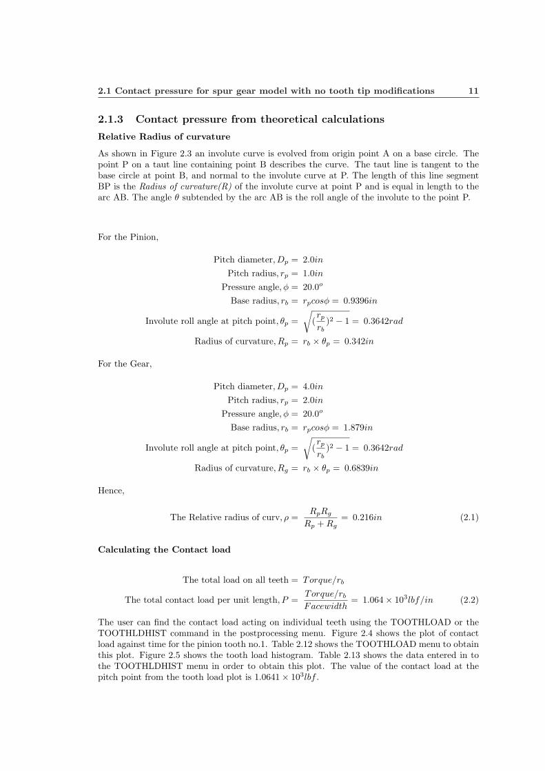
2.1.3 Contact pressure from theoretical calculations
Relative Radius of curvature
As shown in Figure 2.3 an involute curve is evolved from origin point A on a base circle. Thepoint P on a taut line containing point B describes the curve. The taut line is tangent to thebase circle at point B, and normal to the involute curve at P. The length of this line segmentBP is the Radius of curvature(R) of the involute curve at point P and is equal in length to thearc AB. The angle θ subtended by the arc AB is the roll angle of the involute to the point P.
For the Pinion,
Pitch diameter, Dp = 2.0in
Pitch radius, rp = 1.0in
Pressure angle, φ = 20.0o
Base radius, rb = rpcosφ = 0.9396in
Involute roll angle at pitch point, θp =√
(rp
rb)2 − 1 = 0.3642rad
Radius of curvature, Rp = rb × θp = 0.342in
For the Gear,
Pitch diameter, Dp = 4.0in
Pitch radius, rp = 2.0in
Pressure angle, φ = 20.0o
Base radius, rb = rpcosφ = 1.879in
Involute roll angle at pitch point, θp =√
(rp
rb)2 − 1 = 0.3642rad
Radius of curvature, Rg = rb × θp = 0.6839in
Hence,
The Relative radius of curv, ρ =RpRg
Rp + Rg= 0.216in (2.1)
Calculating the Contact load
The total load on all teeth = Torque/rb
The total contact load per unit length, P =Torque/rb
Facewidth= 1.064× 10³lbf/in (2.2)
The user can find the contact load acting on individual teeth using the TOOTHLOAD or theTOOTHLDHIST command in the postprocessing menu. Figure 2.4 shows the plot of contactload against time for the pinion tooth no.1. Table 2.12 shows the TOOTHLOAD menu to obtainthis plot. Figure 2.5 shows the tooth load histogram. Table 2.13 shows the data entered in tothe TOOTHLDHIST menu in order to obtain this plot. The value of the contact load at thepitch point from the tooth load plot is 1.0641× 10³lbf .

12 Calculation of contact pressure for a spur gear model using Calyx
Figure 2.3: Drawing defining the radius of curvature(R) and the roll angle(θ)
Table 2.12: Toothload menu inputs used to obtain the plot of load against time
Item DescriptionSURFACEPAIR PINION SURFACE1 GEAR SURFACE1MEMBER PINIONTOOTHBEGIN 1TOOTHEND 1BEGINSTEP 1ENDSTEP 15
Table 2.13: Toothldhist menu inputs used to obtain the tooth load histogram
Item DescriptionSURFACEPAIR PINION SURFACE1 GEAR SURFACE1MEMBER PINIONTIMESTEP 8HISTCOLOR BLACKAUTOSCALE TRUEOUTPUTTOFILE FALSE

2.1 Contact pressure for spur gear model with no tooth tip modifications 13
-0.8
0000
0-0
.600
000
-0.4
0000
0-0
.200
000
-0.0
0000
00.
2000
000.
4000
000.
6000
000.
8000
00
400.
0000
00
500.
0000
00
600.
0000
00
700.
0000
00
800.
0000
00
900.
0000
00
1000
.000
000
1100
.000
000
Tim
e
Too
th L
oad
on s
urfa
ce p
air:
PIN
ION
_SU
RFA
CE
1_G
EA
R_S
UR
FAC
E1
1.06
4178
E+
003:
Too
th 1
of
PIN
ION
at t
ime=
-2.0
0000
0E-0
01
Figure 2.4: Plot of tooth load against time for pinion tooth no.1

14 Calculation of contact pressure for a spur gear model using Calyx
0.0
200
.0
400
.0
600
.0
800
.0
100
0.0
120
0.0
510
1520
Loa
d on
sur
face
pai
r: P
INIO
N_S
UR
FAC
E1_
GE
AR
_SU
RFA
CE
1
Too
th N
o.
Figure 2.5: Toothload histogram at t=0.0
2.1 Contact pressure for spur gear model with no tooth tip modifications 15
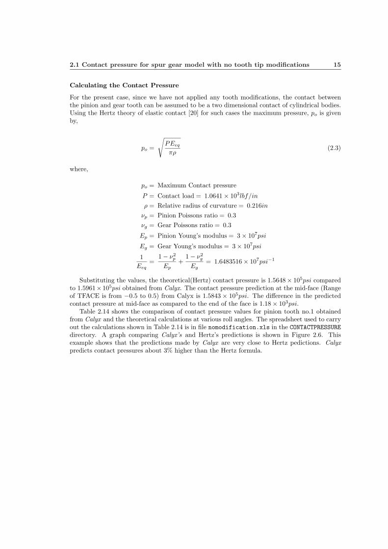
Calculating the Contact Pressure
For the present case, since we have not applied any tooth modifications, the contact betweenthe pinion and gear tooth can be assumed to be a two dimensional contact of cylindrical bodies.Using the Hertz theory of elastic contact [20] for such cases the maximum pressure, po is givenby,
po =
√PEeq
πρ(2.3)
where,
po = Maximum Contact pressure
P = Contact load = 1.0641× 10³lbf/in
ρ = Relative radius of curvature = 0.216in
νp = Pinion Poissons ratio = 0.3νg = Gear Poissons ratio = 0.3
Ep = Pinion Young’s modulus = 3× 10⁷psi
Eg = Gear Young’s modulus = 3× 10⁷psi
1Eeq
=1− ν2
p
Ep+
1− ν2g
Eg= 1.6483516× 10⁷psi−1
Substituting the values, the theoretical(Hertz) contact pressure is 1.5648× 10⁵psi comparedto 1.5961× 10⁵psi obtained from Calyx. The contact pressure prediction at the mid-face (Rangeof TFACE is from −0.5 to 0.5) from Calyx is 1.5843 × 10⁵psi. The difference in the predictedcontact pressure at mid-face as compared to the end of the face is 1.18× 10³psi.
Table 2.14 shows the comparison of contact pressure values for pinion tooth no.1 obtainedfrom Calyx and the theoretical calculations at various roll angles. The spreadsheet used to carryout the calculations shown in Table 2.14 is in file nomodification.xls in the CONTACTPRESSUREdirectory. A graph comparing Calyx’s and Hertz’s predictions is shown in Figure 2.6. Thisexample shows that the predictions made by Calyx are very close to Hertz pedictions. Calyxpredicts contact pressures about 3% higher than the Hertz formula.

16 Calculation of contact pressure for a spur gear model using Calyx
0 2 4 6 8 10 12 140.8
1
1.2
1.4
1.6
1.8
2x 10
5
Time step
Her
tz/C
alyx
con
tact
pre
ssur
e (p
si)
Hertz contact pressureCalyx contact pressure
Figure 2.6: A graph comparing Calyx’s and Hertz’s contact pressure predictions

2.1 Contact pressure for spur gear model with no tooth tip modifications 17
Table 2.14: Contact pressure values obtained from calyx and theoretical calculations for variouspinion roll angles
Time (s) Pinioninvoluterollangle(deg)
Gearinvoluterollangle(deg)
Pinionradiusof curv(in)
Gearradiusof curv(in)
Effectiveradiusof curv(in)
Contactload(lbf/in)
Hertz con-tact pres-sure (psi)
Calyxcontactpressure(psi)
-0.7 8.2539 27.1539 0.1353 0.8906 0.1175 495.34 1.4871 ×10⁵ 1.5243 ×10⁵
-0.6 10.0539 26.2539 0.1648 0.8611 0.1383 526.80 1.4132 ×10⁵ 1.4499 ×10⁵
-0.5 11.8539 25.3539 0.1944 0.8316 0.1575 563.73 1.3700 ×10⁵ 1.3994 ×10⁵
-0.4 13.6539 24.4539 0.2239 0.8021 0.1750 596.79 1.3374 ×10⁵ 1.3611 ×10⁵
-0.3 15.4539 23.5539 0.2534 0.7726 0.1908 629.82 1.3158 ×10⁵ 1.3416 ×10⁵
-0.2 17.2539 22.6539 0.2829 0.7430 0.2049 1064.1 1.6506 ×10⁵ 1.6840 ×10⁵
-0.1 19.0539 21.7539 0.3124 0.7135 0.2173 1064.1 1.6028 ×10⁵ 1.6340 ×10⁵
0.0 20.8539 20.8539 0.3420 0.6840 0.2280 1064.1 1.5648 ×10⁵ 1.5961 ×10⁵
0.1 22.6539 19.9539 0.3715 0.6545 0.2370 1064.1 1.5348 ×10⁵ 1.5683 ×10⁵
0.2 24.4539 19.0539 0.4010 0.6249 0.2442 681.39 1.2097 ×10⁵ 1.2290 ×10⁵
0.3 26.2539 18.1539 0.4305 0.5954 0.2498 568.83 1.0928 ×10⁵ 1.1084 ×10⁵
0.4 28.0539 17.2539 0.4601 0.5659 0.2537 537.37 1.0540 ×10⁵ 1.0715 ×10⁵
0.5 29.8539 16.3539 0.4896 0.5364 0.2559 500.44 1.0128 ×10⁵ 1.0300 ×10⁵
0.6 31.6539 15.4539 0.5191 0.5069 0.2564 467.38 9.7782 ×10⁴ 9.9784 ×10⁴
0.7 33.4539 14.5539 0.5486 0.4773 0.2552 434.35 9.4485 ×10⁴ 9.7802 ×10⁴

18 Calculation of contact pressure for a spur gear model using Calyx
2.2 Contact pressure for spur gear model with linear toothtip modification
Applying a surface modification affects stresses in two ways. Firstly, it changes the load distri-bution between teeth. Secondly, it affects the curvature of the surfaces. This example illustratesthis effect.
2.2.1 The example file
Load the file lineartipmodification.ses from the CONTACTPRESSURE directory.To study the effect of linear tip relief on contact pressure, a linear tip modification is applied
on pinion and gear tooth as shown in Figures 2.7 and 2.8. Tables 2.15 and 2.16 show themodification menus for pinion and gear teeth respectively. All the other menus including thesetup menu are similar to the case with no tooth modifications.
Figure 2.7: Linear tip relief applied to the pinion tooth
Table 2.15: Modification menu for the pinion tooth
Item DescriptionLINEARTIPMOD TRUEROLLLINEARTIPMOD 27.25MAGLINEARTIPMOD 0.0005

2.2 Contact pressure for spur gear model with linear tooth tip modification 19
Figure 2.8: Linear tip relief applied to the gear tooth
Table 2.16: Modification menu for the gear tooth
Item DescriptionLINEARTIPMOD TRUEROLLLINEARTIPMOD 19.60MAGLINEARTIPMOD 0.0005
2.2.2 Obtaining the contact pressure from the postprocessing menu
After the analysis is complete, a post processing data file is created in the working directory.CONTACT command in the postprocessing menu is used to obtain the contact pressure at aparticular instant. Figure 2.9 shows the plot of contact pressure against time for pinion toothno.1. The involute roll angle,θ at the start, θi, and at the tip, θo, of the linear tip relief forthe pinion tooth is 27.25o and 33.68o respectively. At t = 0, the pinion tooth no.1 is in contactwith the gear tooth no.1 at the pitch point. In order to look at the contact pressure valuefor the pinion in the tip relief region a value of θ somewhere between the start and the tip ofthe modified tooth is considered. The contact pressure value from the postprocessing menu att = 0.5s is 1.1832 × 10⁵psi. The exact value of the contact pressure at t=0.5s can be obtainedby plotting the GRIDPRHIST plot as shown in Figure 2.10.

20 Calculation of contact pressure for a spur gear model using Calyx
-0.8
0000
0-0
.600
000
-0.4
0000
0-0
.200
000
-0.0
0000
00.
2000
000.
4000
000.
6000
000.
8000
00
4000
0.00
0000
6000
0.00
0000
8000
0.00
0000
1000
00.0
0000
0
1200
00.0
0000
0
1400
00.0
0000
0
1600
00.0
0000
0
1800
00.0
0000
0
Tim
e
Con
tact
Pre
ssur
e on
sur
face
pai
r: P
INIO
N_S
UR
FAC
E1_
GE
AR
_SU
RFA
CE
1
1.67
7080
E+
005:
Too
th 1
of
PIN
ION
at t
ime=
-2.0
0000
0E-0
01, S
PRO
F=2.
5991
05E
+00
1, T
FAC
E=
-9.
6000
00E
-001
Figure 2.9: Graph of contact pressure against time for pinion tooth no.1

2.2 Contact pressure for spur gear model with linear tooth tip modification 21
Contact Pressure at Time = 5.000000E-001, Range=[0.000000E+000,1.183206E+005]. Each Div.=2.000000E+004
Tooth 1
Figure 2.10: Grid pressure histogram for pinion tooth no.1 at t=0.5s (Contact Pressure at Time= 5.000000E-001s. Range of contact pressure is from 0.000000E+000 to 1.183206E+005 andeach division corresponds to 2.000000E+004

22 Calculation of contact pressure for a spur gear model using Calyx
2.2.3 Obtaining contact pressure from theoretical calculations
Relative Radius of curvature
S.Vijayakar [14] showed that applying tip relief changes the curvature of the surface significantly.The following derivation gives the formula for calculating the curvatures for an involute withlinear tip modification.
If θ is the involute roll angle at a particular point on a involute curve, then the positionvector and its derivatives for a point r(θ) on an unmodified involute curve are given by:
rx(θ) = rb
√1 + θ2(sin(θ − tan−1 θ))
ry(θ) = rb
√1 + θ2(cos(θ − tan−1 θ))
drx
dθ= rbθ(sin(θ))
dry
dθ= rbθ(cos(θ))
d2rx
dθ2= rb(sin(θ) + θ cos(θ))
d2ry
dθ2= rb(cos(θ)− θ sin(θ))
The unit normal vector to the involute and its derivatives are:
nx(θ) = − cos(θ)ny(θ) = + sin(θ)dnx
dθ= +sin(θ)
dny
dθ= +cos(θ)
d2nx
dθ2= +cos(θ)
d2ny
dθ2= − sin(θ)
If e(θ) is the modification for the involute at a particular roll angle θ, E is the magnitude of thelinear modification at the tip, and θi and θo are the roll angles at the start of modification andat the tip, respectively, then the value of linear modification in the relieved part of the involuteis:
e(θ) = Eθ − θi
θo − θi
de
dθ=
E
θo − θi
d2e
dθ2= 0.0
2.2 Contact pressure for spur gear model with linear tooth tip modification 23
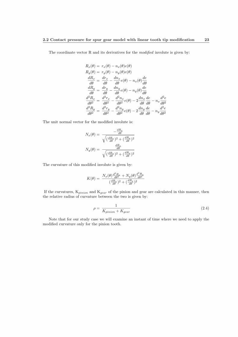
The coordinate vector R and its derivatives for the modified involute is given by:
Rx(θ) = rx(θ)− nx(θ)e(θ)Ry(θ) = ry(θ)− ny(θ)e(θ)dRx
dθ=
drx
dθ− dnx
dθe(θ)− nx(θ)
de
dθdRy
dθ=
dry
dθ− dny
dθe(θ)− ny(θ)
de
dθd2Rx
dθ2=
d2rx
dθ2− d2nx
dθ2e(θ)− 2
dnx
dθ
de
dθ− nx
d2e
dθ2
d2Ry
dθ2=
d2ry
dθ2− d2ny
dθ2e(θ)− 2
dny
dθ
de
dθ− ny
d2e
dθ2
The unit normal vector for the modified involute is:
Nx(θ) =−dRy
dθ√(dRx
dθ )2 + (dRy
dθ )2
Ny(θ) =dRx
dθ√(dRx
dθ )2 + (dRy
dθ )2
The curvature of this modified involute is given by:
K(θ) =Nx(θ)d2Rx
dθ2 + Ny(θ)d2Ry
dθ2
(dRx
dθ )2 + (dRy
dθ )2
If the curvatures, Kpinion and Kgear of the pinion and gear are calculated in this manner, thenthe relative radius of curvature between the two is given by:
ρ =1
Kpinion + Kgear(2.4)
Note that for our study case we will examine an instant of time where we need to apply themodified curvature only for the pinion tooth.

24 Calculation of contact pressure for a spur gear model using Calyx
Calculating the value of θ at 0.5s
Angular velocity of the pinion, ωp = 3.0rpm = 0.31415rad/s.
Therefore,
Rotation of the pinion in 0.5s = 0.5× 0.31415 = 0.1570rad.
At t = 0.0(pitch point), the involute roll angle = 0.36427rad.
Thus,
At t = 0.5s, the pinion involute roll angle, θ = 0.36427 + 0.1570 = 0.5213rad.
At t = 0.5s, the gear involute roll angle, θ = 0.36427− ( rbp
rbg)0.1570 = 0.2854rad.
For the pinion:
Base radius of the pinion is:
rbp = 0.9396in
Involute roll angle at 0.5s is:
θ = 29.85o = 0.5213rad
Involute roll angle at the start of modification is:
θi = 27.21o = 0.475rad
Involute roll angle at the tip of modification is:
θo = 33.68o = 0.588rad
Modification at the tip is:
E = 0.0005in
If e(θ) is the modification for the involute at a roll angle θ = 29.85o, then,
e(θ) = 0.000204inde
dθ= 0.004424in/rad
d2e
dθ2= 0.00

2.2 Contact pressure for spur gear model with linear tooth tip modification 25
The position vector and its derivatives for a point r(θ) on an unmodified involute curve aregiven by:
rx(θ) = 0.043118ry(θ) = 1.058724drx
dθ= 0.243731
dry
dθ= 0.424651
d2rx
dθ2= 0.892422
d2ry
dθ2= 0.571260
The unit normal vector to the involute and its derivatives are:
nx(θ) = −0.867297ny(θ) = 0.497791dnx
dθ= 0.497791
dny
dθ= 0.867297
d2nx
dθ2= 0.867297
d2ny
dθ2= −0.497791
The coordinate vector R and its derivatives for the modified involute is given by:
Rx(θ) = 0.043295Ry(θ) = 1.058622dRx
dθ= 0.247467
dRy
dθ= 0.422272
d2Rx
dθ2= 0.887840
d2Ry
dθ2= 0.563687
The unit vector for the modified involute is:
Nx(θ) = −0.862761Ny(θ) = 0.505611
The curvature of this modified involute is:
Kp = 2.007843in−1
26 Calculation of contact pressure for a spur gear model using Calyx
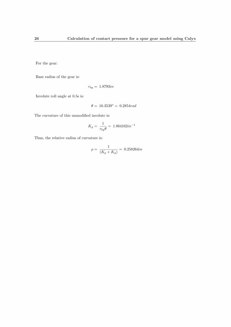
For the gear:
Base radius of the gear is:
rbg = 1.8793in
Involute roll angle at 0.5s is:
θ = 16.3539o = 0.2854rad
The curvature of this unmodified involute is:
Kg =1
rbgθ= 1.864162in−1
Thus, the relative radius of curvature is:
ρ =1
(Kp + Kg)= 0.258264in

2.2 Contact pressure for spur gear model with linear tooth tip modification 27
Calculating the Contact load
The user can find the contact load on individual teeth using the TOOTHLOAD or the TOOTHLD-HIST command in the postprocessing menu. Table 2.17 shows the TOOTHLOAD menu inputsused to obtain the contact load value at t = 0.5s. Figure 2.11 shows the tooth load histogramat t = 0.5s. Table 2.18 shows the TOOTHLDHIST menu inputs used to obtain this plot. Thevalue of contact load at t = 0.5s from the tooth load plot is 6.6757× 10²lbf .
Contact load per unit length =Contact loadFacewidth
= 6.6757× 10²lbf/in (2.5)
Table 2.17: Toothload menu to obtain the contact load at t=0.5s
Item DescriptionSURFACEPAIR PINION SURFACE1 GEAR SURFACE1MEMBER PINIONTOOTHBEGIN 1TOOTHEND 1BEGINSTEP 13ENDSTEP 13
Table 2.18: Toothldhist menu to obtain the tooth load histogram at t=0.5s
Item DescriptionSURFACEPAIR PINION SURFACE1 GEAR SURFACE1MEMBER PINIONTIMESTEP 13HISTCOLOR BLACKAUTOSCALE TRUEOUTPUTTOFILE FALSE

28 Calculation of contact pressure for a spur gear model using Calyx
0.0
100
.0
200
.0
300
.0
400
.0
500
.0
600
.0
700
.0
510
1520
Loa
d on
sur
face
pai
r: P
INIO
N_S
UR
FAC
E1_
GE
AR
_SU
RFA
CE
1
Too
th N
o.
Figure 2.11: Toothload histogram at t=0.5s

2.2 Contact pressure for spur gear model with linear tooth tip modification 29
Calculating the Contact Pressure
For the present case, since we have not applied any lead modifications the contact between thepinion and gear tooth can be assumed to be a two dimensional contact of cylindrical bodies.Using the Hertz theory of elastic contact for such cases the maximum pressure, po is given by,
po =
√PEeq
πρ(2.6)
where,
po = Maximum Contact pressure
P = Contact load per unit length = 6.6757× 10²lbf/in
ρ = Relative radius of curvature = 0.258264in
νp = Pinion Poissons ratio = 0.3νg = Gear Poissons ratio = 0.3
Ep = Pinion Young’s modulus = 3× 10⁷psi
Eg = Gear Young’s modulus = 3× 10⁷psi
1Eeq
=1− ν2
p
Ep+
1− ν2g
Eg
Eeq from above = 1.648351× 10⁷psi
Substituting the above values the theoretical contact pressure is 1.16457× 10⁵psi, comparedwith 1.18321× 10⁵psi predicted by Calyx.
Table 2.19 shows the comparison of contact pressure values for pinion tooth no.1 obtainedfrom Calyx and the Hertz calculations at various roll angles. The spreadsheet used to carry outthe calculations shown in Table 2.19 is in file lineartipmodification.xls in the CONTACTPRESSUREdirectory. A graph comparing Calyx’s and Hertz’s predictions is shown in Figure 2.12. The peakat t = 0.14s corresponding to Invoute angle for gear = 19.60o obtained in the contact pres-sure plot from Calyx is due to the start of the linear modification at the gear tooth. At thispoint the radius of curvature tends to 0.0 and hence we get a high value of contact pressure(1.7650 × 10⁵psi). Hertz formula does not take in to consideration the change in curvature atthe start of modification. Hence we do not see the peak in the contact pressure predictions fromthe Hertz theory. Figure 2.13 shows a plot of contact pressure against time obtained from Calyxin the time range from 0.0s to 0.2s. The peak is clearly seen at t = 0.14s. This example showsthat the predictions made by Calyx are very close to Hertz pedictions.

30 Calculation of contact pressure for a spur gear model using Calyx
−0.8 −0.6 −0.4 −0.2 0 0.2 0.4 0.6 0.80.2
0.4
0.6
0.8
1
1.2
1.4
1.6
1.8x 10
5
Time(s)
Her
tz/C
alyx
con
tact
pre
ssur
e(ps
i)
Hertz contact pressure Calyx contact pressure
Figure 2.12: A graph comparing Calyx’s and Hertz’s contact pressure predictions for linearmodification at the teeth

2.2 Contact pressure for spur gear model with linear tooth tip modification 31
0.00
0000
0.10
0000
0.20
0000
0.30
0000
1500
00.0
0000
0
1600
00.0
0000
0
1700
00.0
0000
0
1800
00.0
0000
0
Tim
e
Con
tact
Pre
ssur
e on
sur
face
pai
r: P
INIO
N_S
UR
FAC
E1_
GE
AR
_SU
RFA
CE
1
1.76
5069
E+
005:
Too
th 1
of
PIN
ION
at t
ime=
1.40
0000
E-0
01, S
PRO
F=3.
2505
61E
+00
1, T
FAC
E=
9.6
0000
0E-0
01
Figure 2.13: A plot of contact pressure against time obtained from Calyx in the time range from0.0s to 0.2s

32 Calculation of contact pressure for a spur gear model using Calyx
Table 2.19: Contact pressure values for linear tip modified tooth obtained from calyx and theo-retical calculations for various pinion roll angles
Time(s) Pinioninvoluterollangle(deg)
Gearinvoluterollangle(deg)
Pinionradiusof curv(in)
Gearradiusof curv(in)
Effectiveradiusof curv(in)
Contactload(lbf/in)
Hertz con-tact pres-sure (psi)
Calyxcontactpressure(psi)
-0.70 8.2539 27.1539 0.1353 0.8975 0.1176 22.015 3.1336 ×10⁴ 4.0065 ×10⁴
-0.60 10.0539 26.2539 0.1648 0.8683 0.1385 154.255 7.6422 ×10⁴ 7.7455 ×10⁴
-0.50 11.8539 25.3539 0.1944 0.8391 0.1578 399.800 1.1528 ×10⁵ 1.1706 ×10⁵
-0.40 13.6539 24.4539 0.2239 0.8099 0.1754 642.476 1.3861 ×10⁵ 1.4057 ×10⁵
-0.30 15.4539 23.5539 0.2534 0.7808 0.1913 872.134 1.5464 ×10⁵ 1.5687 ×10⁵
-0.20 17.2539 22.6539 0.2829 0.7517 0.2055 1064.18 1.6480 ×10⁵ 1.6770 ×10⁵
-0.10 19.0539 21.7539 0.3124 0.7226 0.2181 1064.18 1.5998 ×10⁵ 1.6257 ×10⁵
0.00 20.8539 20.8539 0.3420 0.6935 0.2290 1064.18 1.5612 ×10⁵ 1.5858 ×10⁵
0.02 21.2139 20.6739 0.3479 0.6781 0.2299 1064.18 1.5582 ×10⁵ 1.5749 ×10⁵
0.04 21.5739 20.4939 0.3538 0.6722 0.2318 1064.18 1.5519 ×10⁵ 1.5724 ×10⁵
0.06 21.9339 20.3139 0.3597 0.6663 0.2336 1064.18 1.5460 ×10⁵ 1.5677 ×10⁵
0.08 22.2939 20.1339 0.3656 0.6604 0.2353 1064.18 1.5403 ×10⁵ 1.5712 ×10⁵
0.10 22.6539 19.9539 0.3715 0.6545 0.2370 1064.18 1.5348 ×10⁵ 1.6248 ×10⁵
0.12 23.0139 19.7739 0.3774 0.6486 0.2385 1064.18 1.5297 ×10⁵ 1.7139 ×10⁵
0.14 23.3739 19.5939 0.3833 0.6427 0.2401 1064.18 1.5248 ×10⁵ 1.7650 ×10⁵
0.16 23.7339 19.4139 0.3892 0.6368 0.2415 1064.18 1.5202 ×10⁵ 1.7001 ×10⁵
0.18 24.0939 19.2339 0.3951 0.6309 0.2429 1064.18 1.5159 ×10⁵ 1.5629 ×10⁵
0.20 24.4539 19.0539 0.4010 0.6249 0.2442 1064.18 1.5118 ×10⁵ 1.5428 ×10⁵
0.30 26.2539 18.1539 0.4305 0.5954 0.2498 1042.16 1.4792 ×10⁵ 1.5088 ×10⁵
0.40 28.0539 17.2539 0.4692 0.5659 0.2565 914.303 1.3674 ×10⁵ 1.4261 ×10⁵
0.50 29.8539 16.3539 0.4980 0.5364 0.2582 667.574 1.1645 ×10⁵ 1.1832 ×10⁵
0.60 31.6539 15.4539 0.5269 0.5069 0.2583 423.727 9.2763 ×10⁴ 9.4124 ×10⁴
0.70 33.4539 14.5539 0.5558 0.4773 0.2568 192.965 6.2787 ×10⁴ 6.3045 ×10⁴
2.3 Contact pressure for spur gear model with quadratic tooth tip modification 33
2.3 Contact pressure for spur gear model with quadratictooth tip modification
2.3.1 The example file
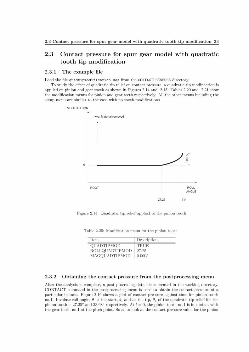
Load the file quadtipmodification.ses from the CONTACTPRESSURE directory.To study the effect of quadratic tip relief on contact pressure, a quadratic tip modification is
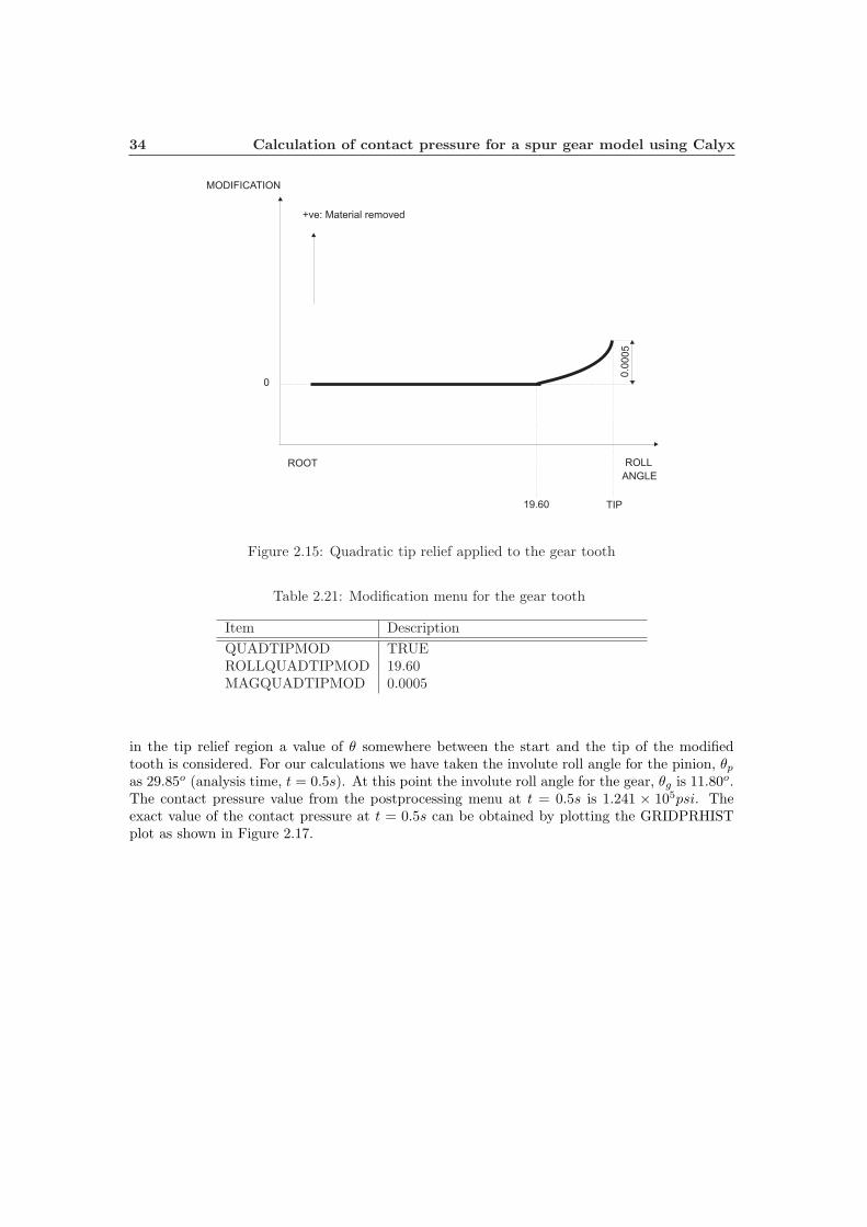
applied on pinion and gear tooth as shown in Figures 2.14 and 2.15. Tables 2.20 and 2.21 showthe modification menus for pinion and gear teeth respectively. All the other menus including thesetup menu are similar to the case with no tooth modifications.
Figure 2.14: Quadratic tip relief applied to the pinion tooth
Table 2.20: Modification menu for the pinion tooth
Item DescriptionQUADTIPMOD TRUEROLLQUADTIPMOD 27.25MAGQUADTIPMOD 0.0005
2.3.2 Obtaining the contact pressure from the postprocessing menu
After the analysis is complete, a post processing data file is created in the working directory.CONTACT command in the postprocessing menu is used to obtain the contact pressure at aparticular instant. Figure 2.16 shows a plot of contact pressure against time for pinion toothno.1. Involute roll angle, θ at the start, θi and at the tip, θo of the quadratic tip relief for thepinion tooth is 27.25o and 33.68o respectively. At t = 0, the pinion tooth no.1 is in contact withthe gear tooth no.1 at the pitch point. So as to look at the contact pressure value for the pinion
34 Calculation of contact pressure for a spur gear model using Calyx
Figure 2.15: Quadratic tip relief applied to the gear tooth
Table 2.21: Modification menu for the gear tooth
Item DescriptionQUADTIPMOD TRUEROLLQUADTIPMOD 19.60MAGQUADTIPMOD 0.0005
in the tip relief region a value of θ somewhere between the start and the tip of the modifiedtooth is considered. For our calculations we have taken the involute roll angle for the pinion, θp
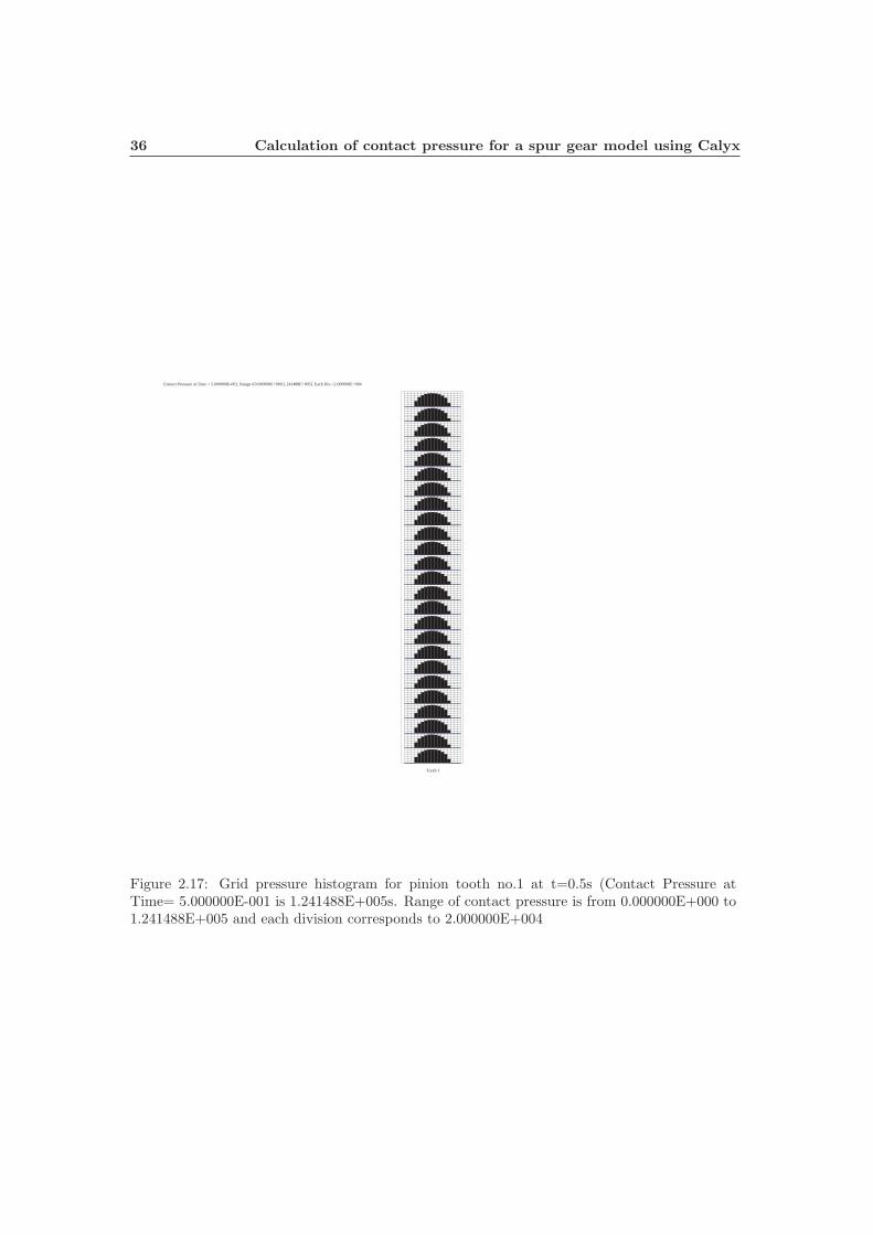
as 29.85o (analysis time, t = 0.5s). At this point the involute roll angle for the gear, θg is 11.80o.The contact pressure value from the postprocessing menu at t = 0.5s is 1.241 × 10⁵psi. Theexact value of the contact pressure at t = 0.5s can be obtained by plotting the GRIDPRHISTplot as shown in Figure 2.17.

2.3 Contact pressure for spur gear model with quadratic tooth tip modification 35
-0.8
0000
0-0
.600
000
-0.4
0000
0-0
.200
000
-0.0
0000
00.
2000
000.
4000
000.
6000
000.
8000
00
4000
0.00
0000
6000
0.00
0000
8000
0.00
0000
1000
00.0
0000
0
1200
00.0
0000
0
1400
00.0
0000
0
1600
00.0
0000
0
1800
00.0
0000
0
Tim
e
Con
tact
Pre
ssur
e on
sur
face
pai
r: P
INIO
N_S
UR
FAC
E1_
GE
AR
_SU
RFA
CE
1
1.69
2024
E+
005:
Too
th 1
of
PIN
ION
at t
ime=
-2.0
0000
0E-0
01, S
PRO
F=2.
5938
07E
+00
1, T
FAC
E=
-9.
6000
00E
-001
Figure 2.16: Plot of contact pressure against time for pinion tooth no.1
36 Calculation of contact pressure for a spur gear model using Calyx
Contact Pressure at Time = 5.000000E-001, Range=[0.000000E+000,1.241488E+005]. Each Div.=2.000000E+004
Tooth 1
Figure 2.17: Grid pressure histogram for pinion tooth no.1 at t=0.5s (Contact Pressure atTime= 5.000000E-001 is 1.241488E+005s. Range of contact pressure is from 0.000000E+000 to1.241488E+005 and each division corresponds to 2.000000E+004

2.3 Contact pressure for spur gear model with quadratic tooth tip modification 37
2.3.3 Contact pressure from theoretical calculations
Relative Radius of curvature
If e(θ) is the quadratic modification for the involute at a particular roll angle θ, E is the mag-nitude of the modification at the tip, and θi and θo are the involute roll angles at the start ofthe modification and at the tip, respectively, then the value of the quadratic modification in therelieved part of the involute is given by:
e(θ) = E(θ − θi
θo − θi)2
de
dθ= 2E
(θ − θi)(θo − θi)2
d2e
dθ2= 2E
1(θo − θi)2
Note that for our study case we will need to apply the modified curvature only for the piniontooth.
For the pinion:
Base radius of the pinion is:
rbp = 0.9396in
Involute roll angle at 0.5s is:
θ = 29.85o = 0.5213rad
Involute roll angle at the start of modification is:
θi = 27.21o = 0.475rad
Involute roll angle at the tip of modification is:
θo = 33.68o = 0.588rad
Modification at the tip is:
E = 0.0005in
If e(θ) is the quadratic modification for the involute at a roll angle θ = 29.85o, then,
e(θ) = 8.3037× 10⁻⁵in
de
dθ= 0.003606in/rad
d2e
dθ2= 0.078314in/(rad)2

38 Calculation of contact pressure for a spur gear model using Calyx
The position vector and its derivatives for a point r(θ) on an unmodified involute curve aregiven by:
rx(θ) = 0.043118ry(θ) = 1.058724drx
dθ= 0.243731
dry
dθ= 0.424651
d2rx
dθ2= 0.892422
d2ry
dθ2= 0.571260
The unit normal vector to the involute and its derivatives are:
nx(θ) = −0.867297ny(θ) = 0.497791dnx
dθ= 0.497791
dny
dθ= 0.867297
d2nx
dθ2= 0.867297
d2ny
dθ2= −0.497791
The coordinate vector R and its derivatives for the modified involute is given by:
Rx(θ) = 0.0431907Ry(θ) = 1.058683dRx
dθ= 0.246818
dRy
dθ= 0.422784
d2Rx
dθ2= 0.956681
d2Ry
dθ2= 0.526062
The unit vector for the modified involute is:
Nx(θ) = −0.863606Ny(θ) = 0.504166
The curvature of this modified involute is:
Kp = 2.340647in−1

2.3 Contact pressure for spur gear model with quadratic tooth tip modification 39
For the gear:
Base radius of the gear is:
rbg = 1.8793in
Involute roll angle at 0.5s is:
θ = 16.3539o = 0.2854rad
The curvature of this unmodified involute is:
Kg =1
rbgθ= 1.864162in−1
Thus, the relative radius of curvature is:
ρ =1
(Kp + Kg)= 0.237823in
40 Calculation of contact pressure for a spur gear model using Calyx
Calculating the Contact load
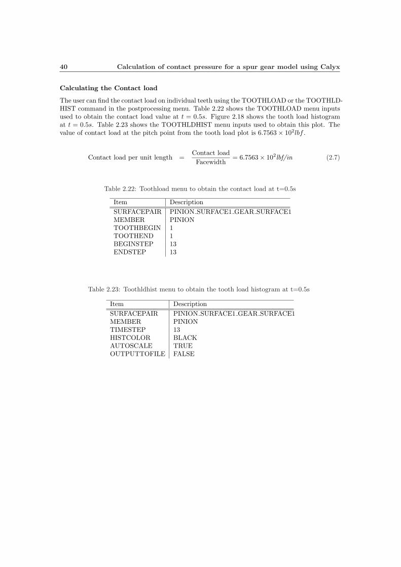
The user can find the contact load on individual teeth using the TOOTHLOAD or the TOOTHLD-HIST command in the postprocessing menu. Table 2.22 shows the TOOTHLOAD menu inputsused to obtain the contact load value at t = 0.5s. Figure 2.18 shows the tooth load histogramat t = 0.5s. Table 2.23 shows the TOOTHLDHIST menu inputs used to obtain this plot. Thevalue of contact load at the pitch point from the tooth load plot is 6.7563× 10²lbf .
Contact load per unit length =Contact loadFacewidth
= 6.7563× 10²lbf/in (2.7)
Table 2.22: Toothload menu to obtain the contact load at t=0.5s
Item DescriptionSURFACEPAIR PINION SURFACE1 GEAR SURFACE1MEMBER PINIONTOOTHBEGIN 1TOOTHEND 1BEGINSTEP 13ENDSTEP 13
Table 2.23: Toothldhist menu to obtain the tooth load histogram at t=0.5s
Item DescriptionSURFACEPAIR PINION SURFACE1 GEAR SURFACE1MEMBER PINIONTIMESTEP 13HISTCOLOR BLACKAUTOSCALE TRUEOUTPUTTOFILE FALSE
2.3 Contact pressure for spur gear model with quadratic tooth tip modification 41
0.0
100
.0
200
.0
300
.0
400
.0
500
.0
600
.0
700
.0
510
1520
Loa
d on
sur
face
pai
r: P
INIO
N_S
UR
FAC
E1_
GE
AR
_SU
RFA
CE
1
Too
th N
o.
Figure 2.18: Toothload histogram at t=0.5s

42 Calculation of contact pressure for a spur gear model using Calyx
Calculating the Contact Pressure
For the present case, since we have not applied any tooth modifications the contact between thepinion and gear tooth can be assumed to be a two dimensional contact of cylindrical bodies.Using the Hertz theory of elastic contact for such cases the maximum pressure, po is given by,
po =PEeq
πρ(2.8)
where,
po = Maximum Contact pressure
P = Contact load per unit length = 6.7563× 10²lbf/in
ρ = Relative radius of curvature = 0.237823in
νp = Pinion Poissons ratio = 0.3νg = Gear Poissons ratio = 0.3
Ep = Pinion Young’s modulus = 3× 10⁷psi
Eg = Gear Young’s modulus = 3× 10⁷psi
1Eeq
=1− ν2
p
Ep+
1− ν2g
Eg
Eeq from above = 1.648351× 10⁷psi
Substituting the above values the theoretical contact pressure is 1.22089× 10⁵psi, comparedwith 1.24148× 10⁵psi predicted by Calyx.
Table 2.24 shows the comparison of contact pressure values for pinion tooth no.1 obtainedfrom Calyx and the theoretical calculations at various roll angles. The spreadsheet used tocarry out the calculations shown in Table 2.24 is in file quadtipmodification.xls in theCONTACTPRESSURE directory. A graph comparing Calyx’s and Hertz’s predictions is shown inFigure 2.19. As can be seen from the plot there is no spike in the contact pressure value whenthe start of modified involute for the gear or pinion comes in contact. This is due to the gradualchange in the curvature of the tooth when you apply quadratic tip modification. This exampleshows that the predictions made by Calyx are very close to Hertz pedictions.

2.3 Contact pressure for spur gear model with quadratic tooth tip modification 43
0 5 10 150.4
0.6
0.8
1
1.2
1.4
1.6
1.8
2x 10
5
Time step
Her
tz/C
alyx
con
tact
pre
ssur
e(ps
i)
Hertz contact pressure Calyx contact pressure
Figure 2.19: A graph comparing Calyx’s and Hertz’s contact pressure predictions for quadraticmodification at the teeth

44 Calculation of contact pressure for a spur gear model using Calyx
Table 2.24: Contact pressure values for quadratic tip modified tooth obtained from calyx andtheoretical calculations for various pinion roll angles
Time(s) Pinioninvoluterollangle(deg)
Gearinvoluterollangle(deg)
Pinionradiusof curv(in)
Gearradiusof curv(in)
Effectiveradiusof curv(in)
Contactload(lbf/in)
Hertz con-tact pres-sure (psi)
Calyxcontactpressure(psi)
-0.7 8.2539 27.1539 0.1353 0.8572 0.1169 64.4317 5.3774 ×10⁴ 5.5576 ×10⁴
-0.6 10.0539 26.2539 0.1648 0.8266 0.1374 193.627 8.5966 ×10⁴ 8.6454 ×10⁴
-0.5 11.8539 25.3539 0.1944 0.7960 0.1562 390.95 1.1457 ×10⁵ 1.1548 ×10⁵
-0.4 13.6539 24.4539 0.2239 0.7654 0.1732 649.995 1.4030 ×10⁵ 1.4206 ×10⁵
-0.3 15.4539 23.5539 0.2534 0.7347 0.1884 960.308 1.6351 ×10⁵ 1.6613 ×10⁵
-0.2 17.2539 22.6539 0.2829 0.7039 0.2018 1064.18 1.6632 ×10⁵ 1.6920 ×10⁵
-0.1 19.0539 21.7539 0.3124 0.6730 0.2134 1064.18 1.6175 ×10⁵ 1.6456 ×10⁵
0.0 20.8539 20.8539 0.3420 0.6420 0.2231 1064.18 1.5818 ×10⁵ 1.6111 ×10⁵
0.1 22.6539 19.9539 0.3715 0.6109 0.2310 1064.18 1.5546 ×10⁵ 1.5873 ×10⁵
0.2 24.4539 19.0539 0.4010 0.6249 0.2442 1064.18 1.5118 ×10⁵ 1.5453 ×10⁵
0.3 26.2539 18.1539 0.4305 0.5954 0.2498 999.747 1.4488 ×10⁵ 1.4789 ×10⁵
0.4 28.0539 17.2539 0.3948 0.5659 0.2325 871.498 1.4021 ×10⁵ 1.4311 ×10⁵
0.5 29.8539 16.3539 0.4272 0.5364 0.2378 675.636 1.2208 ×10⁵ 1.2414 ×10⁵
0.6 31.6539 15.4539 0.4593 0.5069 0.2409 416.723 9.5256 ×10⁴ 9.6432 ×10⁴
0.7 33.4539 14.5539 0.4911 0.4773 0.2420 104.778 4.7655 ×10⁴ 4.7873 ×10⁴

2.4 Contact pressure for spur gear model with lead crown tooth modification 45
2.4 Contact pressure for spur gear model with lead crowntooth modification
When the spur gear teeth are crowned, Hertz’s equations for cylindrical contact can no longerbe used. Hertz’s relationships for elliptical contact need to be used.
2.4.1 The example file
Load the file toothcrowning.ses from the CONTACTPRESSURE directory.To study the effect of crowning on Contact pressure, a lead crown is applied on pinion and
gear tooth as shown in Figures 2.20 and 2.21. Tables 2.25 and 2.26 show the modification menusfor pinion and gear teeth respectively. All the other menus including the setup menu are similarto the case with no tooth modifications.
Figure 2.20: Crowning applied to the pinion tooth
Table 2.25: Modification menu inputs used for the pinion tooth
Item DescriptionLEADCROWN TRUEMAGLEADCROWN 0.0003
46 Calculation of contact pressure for a spur gear model using Calyx
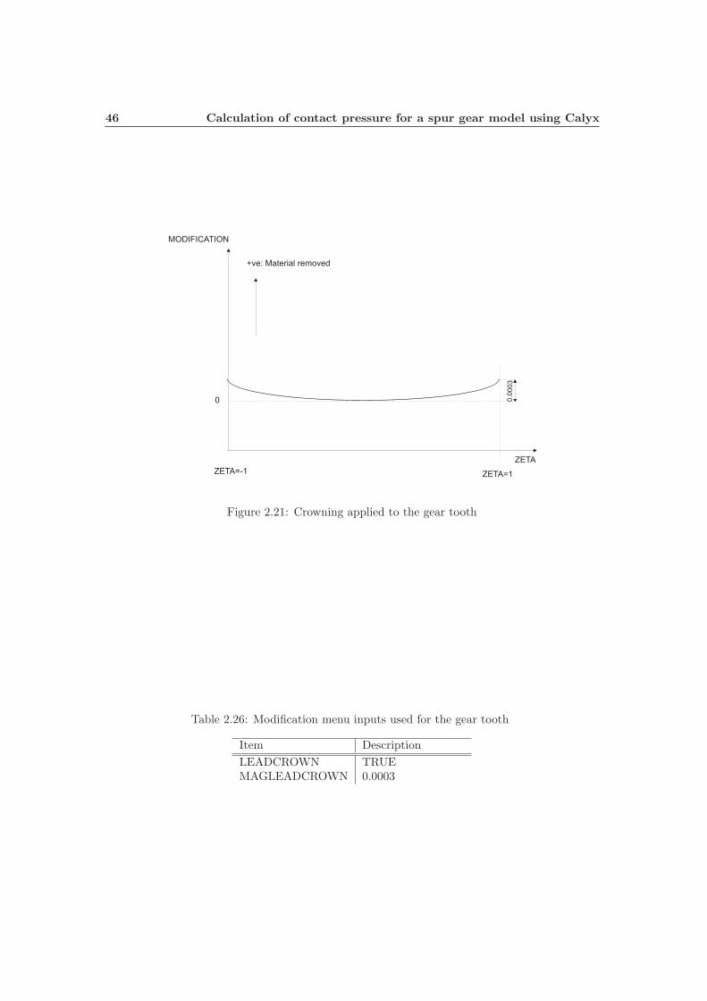
Figure 2.21: Crowning applied to the gear tooth
Table 2.26: Modification menu inputs used for the gear tooth
Item DescriptionLEADCROWN TRUEMAGLEADCROWN 0.0003

2.4 Contact pressure for spur gear model with lead crown tooth modification 47
2.4.2 Obtaining the contact pressure from the postprocessing menu
After the analysis is complete, a post processing data file is created in the working directory.CONTACT command in the postprocessing menu is used to obtain the contact pressure at aparticular instant. Figure 2.22 shows the plot of contact pressure against time for pinion toothno.1. At t = 0, the pinion tooth no.1 is in contact with the gear tooth no.1 at the pitch point.The contact pressure value from the postprocessing menu at t = 0 is 2.0148× 10⁵psi. The exactvalue of the contact pressure at t = 0 can be obtained by plotting the GRIDPRHIST plot asshown in Figure 2.23.

48 Calculation of contact pressure for a spur gear model using Calyx
-0.8
0000
0-0
.600
000
-0.4
0000
0-0
.200
000
-0.0
0000
00.
2000
000.
4000
000.
6000
000.
8000
00
1300
00.0
0000
0
1400
00.0
0000
0
1500
00.0
0000
0
1600
00.0
0000
0
1700
00.0
0000
0
1800
00.0
0000
0
1900
00.0
0000
0
2000
00.0
0000
0
2100
00.0
0000
0
Tim
e
Con
tact
Pre
ssur
e on
sur
face
pai
r: P
INIO
N_S
UR
FAC
E1_
GE
AR
_SU
RFA
CE
1
2.08
9915
E+
005:
Too
th 1
of
PIN
ION
at t
ime=
-2.0
0000
0E-0
01, S
PRO
F=2.
5808
81E
+00
1, T
FAC
E=
-8.
3266
73E
-017
Figure 2.22: Plot of contact pressure against time for pinion tooth no.1

2.4 Contact pressure for spur gear model with lead crown tooth modification 49
Contact Pressure at Time = 0.000000E+000, Range=[0.000000E+000,2.014838E+005]. Each Div.=1.000000E+005
Tooth 1
Figure 2.23: Grid pressure histogram for crowned pinion tooth no.1 at t=0 (Contact Pres-sure at Time= 0.00 is 2.014838E+005. Range of contact pressure is from 0.000000E+000 to2.014838E+005 and each division corresponds to 1.000000E+005
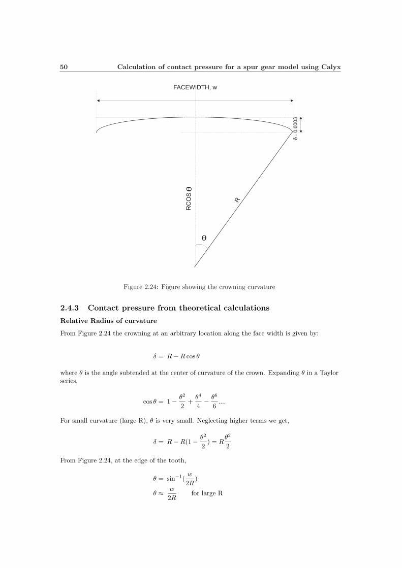
50 Calculation of contact pressure for a spur gear model using Calyx
Figure 2.24: Figure showing the crowning curvature
2.4.3 Contact pressure from theoretical calculations
Relative Radius of curvature
From Figure 2.24 the crowning at an arbitrary location along the face width is given by:
δ = R−R cos θ
where θ is the angle subtended at the center of curvature of the crown. Expanding θ in a Taylorseries,
cos θ = 1− θ2
2+
θ4
4− θ6
6....
For small curvature (large R), θ is very small. Neglecting higher terms we get,
δ = R−R(1− θ2
2) = R
θ2
2
From Figure 2.24, at the edge of the tooth,
θ = sin−1(w
2R)
θ ≈ w
2Rfor large R
2.4 Contact pressure for spur gear model with lead crown tooth modification 51
Therefore,
δ =w2
8R
The Radius of curvature, is therefore,
R =w2
8δ(2.9)
For contact at crowned teeth we assume that the shape of contact is elliptical having semi-axesa and b. To calculate the pressure for such bodies we use the Hertz theory of elastic contact [21]between two general bodies.
If R1 & R′1 denote the principal radii of curvature at the point of contact of one of the bodies,and R2 & R′2 those of the other, and ψ is the angle between the normal planes containing thecurvatures 1/R1 and 1/R2, the constants A and B are determined from the equations:
A + B =12(
1R1
+1
R′1+
1R2
+1
R′2) (2.10)
B −A =12[(
1R1
− 1R′1
)2 + (1
R2− 1
R′2)2
+ 2(1
R1− 1
R′1)(
1R2
− 1R′2
) cos ψ]1/2 (2.11)
For our case we consider R as the radius of curvature in the profile direction and R′ as the radiusof curvature in the facewidth direction. For the case where in the contact is at the pitch point,the radius of curvature in the profile direction for the pinion, R1 = 0.3419in and that for thegear, R2 = 0.6839in. Note that we have already calculated these values in the case where we donot have any tooth modifications. From equation 1.16, the radius of curvature in the facewidthdirection for the pinion, R′1 = 416.67in and that for the gear, R′2 = 416.67in. Also the angle, ψbetween the normal planes containing the curvatures is 0.0.
Substituting the values of R1, R′1, R2, R′2 and ψ in equations for (A + B) and (B - A), we getA + B = 2.1959 and B −A = 2.191.
cosα =B −A
A + B= 0.9977
α = 3.8283o (2.12)
Using the table given for m and n values in Appedix A, by linear interpolation, we get m =13.8577 and n = 0.2150.

52 Calculation of contact pressure for a spur gear model using Calyx
The magnitudes of the semi-axes for the ellipsoid can be calculated using the following:
a = m(3π
4P (kp + kg)(A + B)
)1/3 (2.13)
b = n(3π
4P (kp + kg)(A + B)
)1/3 (2.14)
where,
a, b = semiaxes of the contact regionm,n = constants
P = Contact load per unit lengthνp = Pinion Poissons ratio = 0.3νg = Gear Poissons ratio = 0.3
Ep = Pinion Young’s modulus = 3× 10⁷
Eg = Gear Young’s modulus = 3× 10⁷
kp =1− ν2
p
πEp
kg =1− ν2
g
πEg

2.4 Contact pressure for spur gear model with lead crown tooth modification 53
Table 2.27: Toothload menu inputs used to obtain the contact load at t=0
Item DescriptionSURFACEPAIR PINION SURFACE1 GEAR SURFACE1MEMBER PINIONTOOTHBEGIN 1TOOTHEND 1BEGINSTEP 8ENDSTEP 8
Table 2.28: Toothldhist menu inputs used to obtain the tooth load histogram at t=0
Item DescriptionSURFACEPAIR PINION SURFACE1 GEAR SURFACE1MEMBER PINIONTIMESTEP 8HISTCOLOR BLACKAUTOSCALE TRUEOUTPUTTOFILE FALSE
Calculating the Contact load
The user can find the contact load value using the TOOTHLOAD or the TOOTHLDHISTcommand in the postprocessing menu. Table 2.27 shows the TOOTHLOAD menu to obtain thecontact load value at t = 0. Figure 2.25 shows the tooth load histogram at t = 0. Table 2.28shows the TOOTHLDHIST menu to obtain this plot. The value of contact load at the pitchpoint from the tooth load plot is 1.0641× 10³lbf .

54 Calculation of contact pressure for a spur gear model using Calyx
0.0
200
.0
400
.0
600
.0
800
.0
100
0.0
120
0.0
510
1520
Loa
d on
sur
face
pai
r: P
INIO
N_S
UR
FAC
E1_
GE
AR
_SU
RFA
CE
1
Too
th N
o.
Figure 2.25: Toothload histogram at the t=0

2.5 Conclusion 55
Calculating the Contact Pressure
Using the Hertz theory of elastic contact for elliptical contact the maximum pressure, po is givenby,
po =32
P
πab(2.15)
Calculating a & b and Substituting the value of P from above the theoretical contact pressureis 2.161× 10⁵psi, compared to 2.014× 10⁵psi from the program .
2.5 Conclusion
The difference between the theoretical contact pressure values and those obtained from Calyxis due to the assumption of a very large tooth thickness in the derivations for the Radius ofcurvatures given by the Hertz theory related to contacting bodies. In actual cases the gear bodieshave finite thicknesses. Since Calyx takes in to consideration all the geometrical parameters wefeel that it gives a more accurate representation of the contact pressure values. When youreduce the value of tooth thickness you can see the change in the value of the contact pressure.For tooth thickness=0.15in, the contact pressure value obtained from calyx is 2.003221×10⁵psi.Further reducing the thickness to 0.145in reduces the contact pressure value to 1.993894×10⁵psi.Furthermore, there is error in the analytical predictions because of the error in the values of mand n obtained from linear interpolation.

56 Calculation of contact pressure for a spur gear model using Calyx

Chapter 3
Sub-surface stresses in a spurgear model using Calyx
A verification study comparing the sub-surface stresses predicted by Calyx with those predictedby the theory of elasticity is presented here.
3.1 The spur gear model with no tooth modification
This example uses an unmodified spur gear .
3.1.1 The example file
After hitting the CONNECT button, choose the CONTACTPRESSURE directory under the SAMPLESdirectory. This in turn is located in the Working directory(WORKDIR) selected by the User at theinstallation time. Load the file subsurface.ses from the CONTACTPRESSURE directory.
This session file contains a model identical to the spur gear set described in the previouschapter. The only difference is that only one time step will be analyzed. We have chosen toanalyze the gear pair at the pitch point.
Tables 3.1 shows the analysis setup.
3.1.2 Obtaining the sub-surface stress from the postprocessing menu
During the analysis, a post processing data file is created in the working directory. The SUB-SURFACE command in the postprocessing menu is used to obtain the sub-surface stress at aparticular instant. At t = 0, the pinion tooth no.1 is in contact with the gear tooth no.1 atthe pitch point. Figure 3.1 shows the sub-surface Von-Mises stress as a function of depth. Ta-ble 3.2 shows the inputs used to obtain this plot. The SUBSURFACE command selects thegrid cell with the maximum contact pressure as the location for sub-surface stress computation.We restricted ourselves to the middle of the face width by setting TFACEBEGIN = -0.01 andTFACEEND = +0.01. The depth was varied from 0.00001 inch to 0.02 inch. A total of 101points were sampled. The predicted maximum Von Mises stress is 41,529 psi at a depth of 0.003inches, and the maximum shear stress is 47,551 psi at a depth of 0.0034 inches. The maximumshear stress predicted by the theory of elasticity is 47,928 psi at the same depth. Figure 3.2shows the maximum shear as a function of depth.
Figures 3.3 through 3.6 show the comparison between Calyx and theory (K. L. Johnson [20]) ofthe normal stresses and maximum shear stress as a function of depth. An excel file subsurface.xlscontaining the theory of elasticity calculations can be found in the CONTACTPRESSURE directory.

58 Sub-surface stresses in a spur gear model using Calyx
Table 3.1: Setup menu inputs
Item DescriptionSEPTOL 0.05NPROFDIVS 8NFACEDIVS 25DSPROF 0.0005ZEROINITIAL TRUEINITIALTIME -0.1NRANGES 1RANGE 1SOLMETHOD STATICNTIMESTEPS 1DELTATIME 0.1STARTSPEEDFACTOR 1.0STARTTORQUEFACTOR 1.0ENDTORQUEFACTOR 1.0SAVEPERIODICALLY FALSEOUTPUTRESTART FALSEPOSTPROCWRITE TRUEPOSTFILENAME postproc.datNSTEPSWRITE 1
Table 3.2: Sub-surface menu inputs
Item DescriptionSURFACEPAIR PINION SURFACE1 GEAR SURFACE1MEMBER PINIONTOOTHBEGIN 1TOOTHEND 1TIMESTEP 1SPROFBEGIN 0.0SPROFEND 48.0TFACEBEGIN -0.01TFACEEND 0.01DEPTHBEGIN 0.00001DEPTHEND 0.02NUMDEPTH 101COMPONENT VONMISESOUTPUTTOFILE FALSE

3.1 The spur gear model with no tooth modification 59
0.00
0000
0.00
2000
0.00
4000
0.00
6000
0.00
8000
0.01
0000
0.01
2000
0.01
4000
0.01
6000
0.01
8000
0.02
0000
1000
0.00
0000
2000
0.00
0000
3000
0.00
0000
4000
0.00
0000
5000
0.00
0000
Dep
th
Von
Mis
es S
tres
s (s
vm)
4.15
2929
E+
004:
Too
th 1
at d
epth
=3.
0085
00E
-003
, s=
2.94
4747
E+
001,
t=2.
9447
47E
+00
1 (c
onta
ct p
ress
ure=
1.58
3446
E+
005)
Figure 3.1: Graph of sub-surface Von Mises stress as a function of depth at pinion tooth no.1.The contact is at the pitch point.

60 Sub-surface stresses in a spur gear model using Calyx
0.00
0000
0.00
2000
0.00
4000
0.00
6000
0.00
8000
0.01
0000
0.01
2000
0.01
4000
0.01
6000
0.01
8000
0.02
0000
1000
0.00
0000
2000
0.00
0000
3000
0.00
0000
4000
0.00
0000
5000
0.00
0000
Dep
th
Max
She
ar (
s3-s
1)/2
4.75
5080
E+
004:
Too
th 1
at d
epth
=3.
4083
00E
-003
, s=
2.94
4747
E+
001,
t=2.
9447
47E
+00
1 (c
onta
ct p
ress
ure=
1.58
3446
E+
005)
Figure 3.2: Graph of sub-surface max. shear stress as a function of depth at pinion toothno.1.The contact is at the pitch point.

3.1 The spur gear model with no tooth modification 61
Sigma xx
-180000
-160000
-140000
-120000
-100000
-80000
-60000
-40000
-20000
0
0.00E+00 5.00E-03 1.00E-02 1.50E-02 2.00E-02 2.50E-02
Calyx sxx
Hertz sxx
Figure 3.3: Comparison of sub-surface σxx predicted by Calyx with that computed by the theoryof elasticity (K. L. Johnson [20]).
Sigma yy
-120000
-100000
-80000
-60000
-40000
-20000
0
0.00E+00 5.00E-03 1.00E-02 1.50E-02 2.00E-02 2.50E-02
Calyx syy
Hertz syy
Figure 3.4: Comparison of sub-surface σyy predicted by Calyx with that computed by the theoryof elasticity (K. L. Johnson [20]).

62 Sub-surface stresses in a spur gear model using Calyx
Sigma zz
-200000
-180000
-160000
-140000
-120000
-100000
-80000
-60000
-40000
-20000
0
0.00E+00 5.00E-03 1.00E-02 1.50E-02 2.00E-02 2.50E-02
Calyx szz
Hertz szz
Figure 3.5: Comparison of sub-surface σzz predicted by Calyx with that computed by the theoryof elasticity (K. L. Johnson [20]).
Tau_max=(sxx-szz)/2
0
10000
20000
30000
40000
50000
60000
0.00E+00 5.00E-03 1.00E-02 1.50E-02 2.00E-02 2.50E-02
Calyx MaxShear=(sxx-szz)/2
Hertz Maxshear
Figure 3.6: Comparison of sub-surface τmax = (σxx − σzz)/2 predicted by Calyx with thatcomputed by the theory of elasticity (K. L. Johnson [20]).

Chapter 4
Calculation of transmission errorfor a spur and helical gear modelusing Calyx
4.1 Introduction
Gear noise is mainly characterized by components at the gear mesh frequency and its multiples.The gear mesh frequency is the inverse of the time period between consecutive tooth contact andmay be computed multiplying the number of teeth on the gear by its rotational velocity. Otherfrequency components can also occur, but they are usually secondary with respect to the meshfrequency. The most important exciters of the gear forces, which are periodic at the gear meshfrequency are:
• Transmission error
• Mesh stiffness changes
If gears were perfect involutes, absolutely rigid and correctly spaced, there would be novibration generated when meshing. In practice, for a variety of reasons, this does not occurand the idea of transmission error came into existence. The transmission error is defined as thedifference between the current position of the output gear and the position it would occupy ifit were perfectly conjugated with the input gear. For unloaded gears, transmission error is theresult of surface modifications and manufacturing inaccuracies such as profile errors, spacingerrors and runout. For loaded gears, the teeth deflection due to the mesh stiffness variation,superimposed to the unloaded gear errors, is the cause of the transmission error.
A vibration transmission path starts from a combination of manufacturing errors and toothand gear deflections to generate the transmission error. The transmission error is then the sourceof vibration and it drives the internal dynamics of the gears to give vibration forces through thebearing supports. In turn, these bearing forces drive the external gear case vibration or, via anyisolation mounts, drive the external structure to find the sound radiating panel which transmitsnoise. In a vehicle, after the vibration has travelled from the gear box through the engine maincasting to the support mounts and hence to the structure, it may travel several meters in thebody before exciting a panel to emit sound that annoys the occupants.

64 Calculation of transmission error for a spur and helical gear model using Calyx
Table 4.1: Data for low contact ratio spur gear
Item Pinion GearNUMBER OF TEETH 20 119TRANSVERSE DIAM. PITCH (in−1) 7.8 7.8TRANSVERSE PRESSURE ANGLE (deg) 20.0 20.0CENTER DISTANCE (in) 8.9102 8.9102OPERATING PITCH DIAM. (in) 2.56409 15.2563OUTSIDE PITCH DIAM. (in) 2.82050 15.4927ROOT DIAM. (in) 2.19486 14.8671INNER DIAM. (in) 1.20 13.90FACE WIDTH (in) 1.0 1.0STANDARD PITCH RADIUS (in) 0.201382 0.19410OPERATING PITCH RADIUS (in) 0.201382 0.19410CONTACT RATIO 1.6443 1.6443TORQUE (lbf − in) 1000 5950
4.2 Measuring the transmission error using calyx
A. Singh [22] in his Masters thesis made a comparison between the transmission error valuespredicted by the Contact Analysis Program Package called CAPP and the Load DistributionProgram called LDP developed at The Ohio State University. In this chapter we have comparedthe transmission error values obtained from Calyx with these results.
4.2.1 Comparison of transmission error values obtained from Calyxand LDP for Spur gears
Two sets of spur gears are analysed. The first is a low contact ratio spur gear and is described inTable 4.1. Load the file tespurlowcr.ses from the TRANSERROR directory in the Working direc-tory(WORKDIR). Figure 4.1 shows the transmission error curves obtained from LDP and CAPPfor this gear set. Figure 4.2 shows the transmission error plot for the gear set obtained usingCalyx. This plot is obtained using the BODYDEFLECTION command in the postprocessingmenu. The peak to peak transmission error(T.E) which is the difference in the maximum deflec-tion and the minimum deflection in the Z-direction is 1.50132 × 10⁻⁴rads = 180.86µin (Usinga base radius value of 1.204728in). Figure 4.3 shows the same T.E curve in µin. The sign usedfor the transmission error is opposite to that used in Figure 4.1. LDP predicts a peak to peakT.E value of 190µin. CAPP predicts a peak to peak T.E of 150µin.

4.2 Measuring the transmission error using calyx 65
Figure 4.1: Comparison of transmission error predicted by LDP and CAPP for a low contactratio spur gear model under a load of 1000lbf − in. Peak to Peak transmission error obtainedfrom LDP is about 190µin. CAPP predicts a peak to peak T.E of 150µin. (From “Analysisof spur and helical gears using a combination of finite element and surface integral techniques”,M.S. Thesis by Avinashchandra Singh at The Ohio State University).

66 Calculation of transmission error for a spur and helical gear model using Calyx
-0.6
0000
0-0
.400
000
-0.2
0000
0-0
.000
000
0.20
0000
0.40
0000
0.60
0000
-0.0
0042
0
-0.0
0040
0
-0.0
0038
0
-0.0
0036
0
-0.0
0034
0
-0.0
0032
0
-0.0
0030
0
-0.0
0028
0
-0.0
0026
0
-0.0
0024
0
Tim
e
Bod
y Fr
ame
defl
ectio
n T
HE
TA
Z
TH
ET
AZ
, Ran
ge=
[-4.
1068
10E
-004
,-2.
6054
90E
-004
], P
eak
to P
eak=
1.50
1320
E-0
04
Figure 4.2: Transmission error predicted by Calyx for a low contact ratio spur gear model undera load of 1000lbf−in. Peak to Peak transmission error predicted by Calyx is 1.50132×10⁻⁴rads.

4.2 Measuring the transmission error using calyx 67
−0.8 −0.6 −0.4 −0.2 0 0.2 0.4 0.6−500
−480
−460
−440
−420
−400
−380
−360
−340
−320
−300
Time(s)
Tra
nsm
issi
on e
rror
(µ in
)
Figure 4.3: Transmission error predicted by Calyx for a low contact ratio spur gear model undera load of 1000lbf − in. Peak to Peak transmission error obtained from Calyx is about 180µin.

68 Calculation of transmission error for a spur and helical gear model using Calyx
Table 4.2: Data for a high contact ratio spur gear
Item Pinion GearNUMBER OF TEETH 27 34TRANSVERSE DIAM. PITCH (in−1) 10.233 10.233TRANSVERSE PRESSURE ANGLE (deg) 20.811 20.811CENTER DISTANCE (in) 2.980 2.980OPERATING PITCH DIAM. (in) 2.63803 3.32197OUTSIDE PITCH DIAM. (in) 2.885 3.622ROOT DIAM. (in) 2.320 3.039INNER DIAM. (in) 1.5 2.0FACE WIDTH (in) 1.152 1.152STANDARD PITCH RADIUS (in) 0.142 0.160OPERATING PITCH RADIUS (in) 0.142159 0.160203CONTACT RATIO 2.17 2.17TORQUE (lbf − in) 900 1133.33
The data for a high contact ratio spur gear is described in Table 4.2. Load the file tespurhighcr.sesfrom the TRANSERROR directory in the Working directory(WORKDIR). Figure 4.4 shows the trans-mission error curves obtained from LDP and CAPP for this gear set. Figure 4.5 shows the T.Ecurve in µin obtained from Calyx. The peak to peak T.E predicted by CAPP is approximately35µin. LDP predicts approximately 50µin. Calyx predicts a peak to peak T.E of 37.4µin witha base radius of 1.232959in.

4.2 Measuring the transmission error using calyx 69
Figure 4.4: Comparison of transmission error predicted by LDP and CAPP for a high contactratio spur gear model under a load of 900lbf − in. Peak to Peak transmission error obtainedfrom LDP is about 50µin. (From “Analysis of spur and helical gears using a combination offinite element and surface integral techniques”, M.S. Thesis by Avinashchandra Singh at TheOhio State University).

70 Calculation of transmission error for a spur and helical gear model using Calyx
−0.4 −0.3 −0.2 −0.1 0 0.1 0.2 0.3 0.4165
170
175
180
185
190
195
200
205
Time(s)
Tra
nsm
issi
on e
rror
(µ in
)
Figure 4.5: Transmission error predicted by Calyx for a low contact ratio spur gear model undera load of 900lbf − in. Peak to Peak transmission error obtained from Calyx is 37.411µin.

4.3 Conclusion 71
Table 4.3: Data for a helical gear set
Item Pinion GearNUMBER OF TEETH 13 127NORMAL DIAM. PITCH (in−1) 6.173435 6.173435TRANSVERSE DIAM. PITCH (in−1) 5.29167 5.29167TRANSVERSE PRESSURE ANGLE (deg) 23.00704 23.00704NORMAL PRESSURE ANGLE (deg) 20.0 20.0HELIX ANGLE (deg) 31.00 31.00CENTER DISTANCE (in) 13.22835 13.22835PITCH DIAM. (in) 2.4567 24.00OUTSIDE DIAM. (in) 2.9637 24.2278ROOT DIAM. (in) 2.1202 23.3842INNER DIAM. (in) 0.90 22.00FACE WIDTH (in) 2.00 2.00TRANSVERSE CIRCULAR THICKNESS (in) 0.341357 0.234960FACE CONTACT RATIO 2.0242 2.0242TRANSVERSE CONTACT RATIO 1.3944 1.3944TORQUE (lbf − in) 8040.0 78544.6
4.2.2 Comparison of transmission error values obtained from Calyxand LDP for Helical gears
The data for a helical gear set is described in Table 4.3. Load the file tehelical.ses fromthe TRANSERROR directory in the Working directory(WORKDIR). Figure 4.6 shows the transmissionerror curves obtained from LDP and CAPP for this gear set. The T.E curve obtained fromCAPP in Figure 4.6 seems to be wrong. Figure 4.7 shows the T.E curve obtained from a morerecent run made with CAPP. Note that the sign convention used for this model is opposite tothat shown in Figure 4.6. Figure 4.8 shows the T.E curve in µin obtained from Calyx. The peakto peak T.E predicted by CAPP is 23.40µin. LDP predicts aproximately 40µin. Calyx predictsa peak to peak T.E of 27.745µin with a base radius of 1.130643in.
4.3 Conclusion
The deflection curve obtained from Calyx closely matches with that obtained from LDP andCAPP. LDP does not predict the premature contact of the gear teeth due to deflection underload because of the assumption of contact along the line of action. The contact ratio obtainedfrom LDP is the theoretical contact ratio. So, the transmission error obtained from LDP has asudden jump when the gears go from one pair of teeth to two pairs of teeth in contact. But theT.E curve obtained from CAPP and Calyx has a smooth transition from one pair of teeth to twopairs of teeth in contact. Thus Calyx gives a reasonably correct representation of transmissionerror for both spur and helical gears.
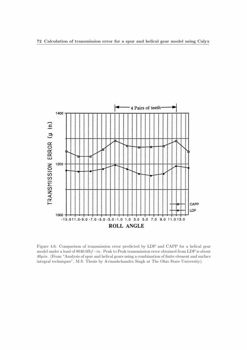
72 Calculation of transmission error for a spur and helical gear model using Calyx
Figure 4.6: Comparison of transmission error predicted by LDP and CAPP for a helical gearmodel under a load of 8040.0lbf−in. Peak to Peak transmission error obtained from LDP is about40µin. (From “Analysis of spur and helical gears using a combination of finite element and surfaceintegral techniques”, M.S. Thesis by Avinashchandra Singh at The Ohio State University).

4.3 Conclusion 73
-20
.0 -
10.0
0.
0 1
0.0
20.
0
-0.
0716
-0.
0714
-0.
0712
-0.
0710
-0.
0708
-0.
0706
-0.
0704
-0.
0702
Rol
l Ang
le (
Deg
)
Tra
ns. E
rror
The
ta_Z
at G
ear
1 (D
egre
es):
Max
=-0
.702
8E-0
1, M
in=
-0.7
147E
-01,
Pea
k to
pea
k= 0
.118
6E-0
2
Tra
nsm
issi
on E
rror
Figure 4.7: Transmission error predicted by CAPP for a helical gear model under a load of8040lbf − in. Peak to Peak transmission error obtained from CAPP is 23.40µin.

74 Calculation of transmission error for a spur and helical gear model using Calyx
0 0.2 0.4 0.6 0.8 1 1.2 1.4 1.6 1.81525
1530
1535
1540
1545
1550
1555
1560
Time(s)
Tra
nsm
issi
on e
rror
(µ in
)
Figure 4.8: Transmission error predicted by Calyx for a low contact ratio spur gear model undera load of 8040lbf − in. Peak to Peak transmission error obtained from Calyx is 27.75µin.

Chapter 5
Internal helical gear pair example
The internal helical gear set example will help the user model an internal helical gear pair usingthe Helical3D program. Figure 5.1 shows the finite element model of a internal helical gear set.
5.1 The example file
Load the file internal.ses from the EXAMPLES directory under the SAMPLES directory.The example model does not have any tooth modifications on the pinion or the gear.Tables 5.2 through 5.11 show the data to be entered in the EDIT menu for running the
internal gear model. No assembly errors are considered for the pinion and the ring/gear. Alsothere are no bearings in the model.

76 Internal helical gear pair example
Figure 5.1: Finite element model of an internal helical gear set
Table 5.1: Units used for the internal helical gear set
Physical quantity EnglishLENGTH inTIME secsANGLE deg or radMASS lbf.s2/inMOMENT OF INERTIA lbf.s2.inSTIFFNESS lbf/inSPEED RPM or rad/secTORQUE lbf.inYOUNGS MODULUS lbf/in2
DENSITY lbf.s2/in4
LOAD lbfSTRESSES psi

5.1 The example file 77
Table 5.2: System configuration parameters
Item DescriptionMESHTYPE CALYX3DCENTERDIST 3.02OFFSET 0.00ROTX 0.00ROTY 0.00INPUT PINIONTORQUEINPUT 1000.00RPMINPUT -3.00MU 0.00MAGRUNOUTGEAR 0.00ANGRUNOUTGEAR 0.00MAGRUNOUTPINION 0.00ANGRUNOUTPINION 0.00BACKSIDECONTACT FALSE
Table 5.3: Pinion data
Item DescriptionLUMPMASS 0.00LUMPMOMINERTIA 0.00LUMPALPHA 0.00
Table 5.4: Pinion tooth data
Item DescriptionNTEETH 20NFACEELEMS 4COORDORDER 10DISPLORDER 3PLANE TRANSVERSEXVERSEDIAMPITCH 10XVERSEPRESSANGLE 20XVERSETHICK 0.15708FACEWIDTH 1HAND LEFTHELIXANGLE 20.00RACKTIPRAD 0.02OUTERDIA 2.18ROOTDIA 1.70RIMDIA 1.40YOUNGSMOD 3x10⁷
POISSON 0.3MSHFILE pinion.mshTPLFILE medium.tpl

78 Internal helical gear pair example
Table 5.5: Pinion rim data
Item DescriptionRIMTYPE SIMPLERIMDIA 1.40INNERDIA 1.20WIDTH 1.00OFFSET 0.00AXIALORDER 2CIRCORDER 8ELEMTYPE LINEARNDIVSRADIAL 2NTHETA 32NDIVSWIDTH 4
Table 5.6: Pinion bearing menu
Item DescriptionRIGIDRACE FALSECIRCORDER 8AXIALORDER 2BEARING FALSE
Table 5.7: Gear data
Item DescriptionTYPE INTERNALLUMPMASS 0.00LUMPMOMINERTIA 0.00LUMPALPHA 0.00

5.1 The example file 79
Table 5.8: Gear tooth data
Item DescriptionNTEETH 80NFACEELEMS 4COORDORDER 10DISPLORDER 3PLANE TRANSVERSEXVERSEDIAMPITCH 10XVERSEPRESSANGLE 20XVERSETHICK 0.14FACEWIDTH 1HAND LEFTHELIXANGLE 20.00RACKTIPRAD 0.04OUTERDIA 7.80ROOTDIA 8.30RIMDIA 8.65YOUNGSMOD 3x10⁷
POISSON 0.3MSHFILE gear.mshTPLFILE medium.tpl
Table 5.9: Gear rim data
Item DescriptionRIMTYPE SIMPLERIMDIA 8.65OUTERDIA 9.00WIDTH 1.00OFFSET 0.00AXIALORDER 2CIRCORDER 16ELEMTYPE QUADRATICNDIVSRADIAL 4NTHETA 64NDIVSWIDTH 4
Table 5.10: Gear bearing menu
Item DescriptionRIGIDRACE FALSECIRCORDER 16AXIALORDER 2BEARING FALSE
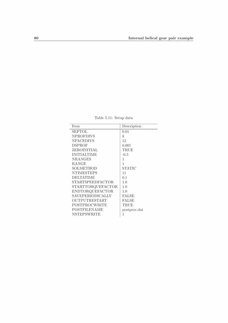
80 Internal helical gear pair example
Table 5.11: Setup data
Item DescriptionSEPTOL 0.01NPROFDIVS 8NFACEDIVS 12DSPROF 0.001ZEROINITIAL TRUEINITIALTIME -0.5NRANGES 1RANGE 1SOLMETHOD STATICNTIMESTEPS 11DELTATIME 0.1STARTSPEEDFACTOR 1.0STARTTORQUEFACTOR 1.0ENDTORQUEFACTOR 1.0SAVEPERIODICALLY FALSEOUTPUTRESTART FALSEPOSTPROCWRITE TRUEPOSTFILENAME postproc.datNSTEPSWRITE 1

5.2 Results 81
Figure 5.2: Maximum principal normal stress contour for an internal helical gear set
5.2 Results
After the analysis is complete a postprocessing file is created in the working directory. Figure 5.2shows the maximum principal normal stress contour for the internal helical gear pair.

82 Internal helical gear pair example

Chapter 6
Internal helical gear with webbedrim
Figure 6.1 shows the finite element model of a internal helical gear set with webbed rim .
6.1 The example file
Load the file internalwebbed.ses from the EXAMPLES directory.The data is similar to the previous example except for the rim menu. The example model
does not have any tooth modifications on the pinion or the gear.
6.2 Modeling the rim
The purpose of including a rim model is to apply the correct boundary conditions to the toothmodel. This is important because the boundary conditions can have a significant effect on theload and stress distribution.
The webbed rim is composed of an arbitrary number of ‘segments’(in this case 4). Theposition of the first segment cannot be changed. As discussed in the Users manual each of theremaining segments can be placed in four different positions(AHEAD, BEHIND, INSIDE andOUTSIDE) relative to the previous segment.
Table 6.1 shows the data common to all the segments for the webbed rim for the internalgear. Table 6.2 show the radial and axial coordinates for each segment and their respectivepositions relative to the previous segment.
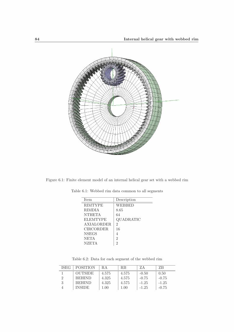
84 Internal helical gear with webbed rim
Figure 6.1: Finite element model of an internal helical gear set with a webbed rim
Table 6.1: Webbed rim data common to all segments
Item DescriptionRIMTYPE WEBBEDRIMDIA 8.65NTHETA 64ELEMTYPE QUADRATICAXIALORDER 2CIRCORDER 16NSEGS 4NETA 2NZETA 2
Table 6.2: Data for each segment of the webbed rim
ISEG POSITION RA RB ZA ZB1 OUTSIDE 4.575 4.575 -0.50 0.502 BEHIND 4.325 4.575 -0.75 -0.753 BEHIND 4.325 4.575 -1.25 -1.254 INSIDE 1.00 1.00 -1.25 -0.75

6.3 Results 85
Figure 6.2: Maximum principal normal stress contour for an internal helical gear set with awebbed rim
6.3 Results
After the analysis is complete a postprocessing file is created in the working directory. Figure 6.2shows the maximum principal normal stress contour for the internal helical gear pair.

86 Internal helical gear with webbed rim

Chapter 7
Modeling splines using theHelical 3D program
Using the Helical3D program external splines or internal splines can be used with external orinternal gears. Thus it is possible to model four different combinations of gears and splines.
7.1 Internal splines on external gear
The following example has internal splines on an external gear(Pinion). Figure 7.1 shows themodel of a internal helical gear set with splines on the inner diameter of the Pinion .
7.1.1 The example file
Load the file extgearintsplines.ses from the EXAMPLES directory.The data is similar to the Internal helical gear pair example except for the pinion rim menu.
The example model does not have any tooth modifications on the pinion or the gear.
7.1.2 Modeling the splines
The INTERNALSPLINED option in the Rim menu refers to the internal splines. The pinionrim data to model the internal splines on the pinion is shown in Table 7.1. All the splines areevenly spaced along the inner diameter of the pinion.
7.1.3 Results
After the analysis is complete a postprocessing file is created in the working directory. Figure 7.2shows the maximum principal normal stress contour for the internal helical gear pair. Figure 7.3shows the load distribution on the pinion and the splines.

88 Modeling splines using the Helical 3D program
Figure 7.1: An internal helical gear set with internal splines on the external gear
Figure 7.2: Maximum principal normal stress contour for an internal helical gear set with internalsplines on the pinion

7.1 Internal splines on external gear 89
Table 7.1: Pinion rim menu to model the internal splines
Item DescriptionRIMTYPE INTERNALSPLINEDTYPE DOUBLESIDEDBACKLASH 0.00RIMDIA 1.40INNERDIA 1.20RIMWIDTH 1.00RIMOFFSET 0.00AXIALORDER 2CIRCORDER 8ELEMTYPE LINEARNDIVSRADIAL 2NTHETA 32NDIVSWIDTH 4NSPLINES 8PRESSANGLE 10SPLINEWIDTH 0.15SPLINEHEIGHT 0.10SPLINELENGTH 0.35SPLINEOFFSET 0.15EVEN TRUEANGPOSNFIRSTSPLIN 0.00SPLINEELEMTYPE QUADRATICNDIVSSPLINEWIDTH 2NDIVSSPLINEHEIGHT 2NDIVSSPLINELENGTH 2

90 Modeling splines using the Helical 3D program
Figure 7.3: Load distribution on the pinion and the splines
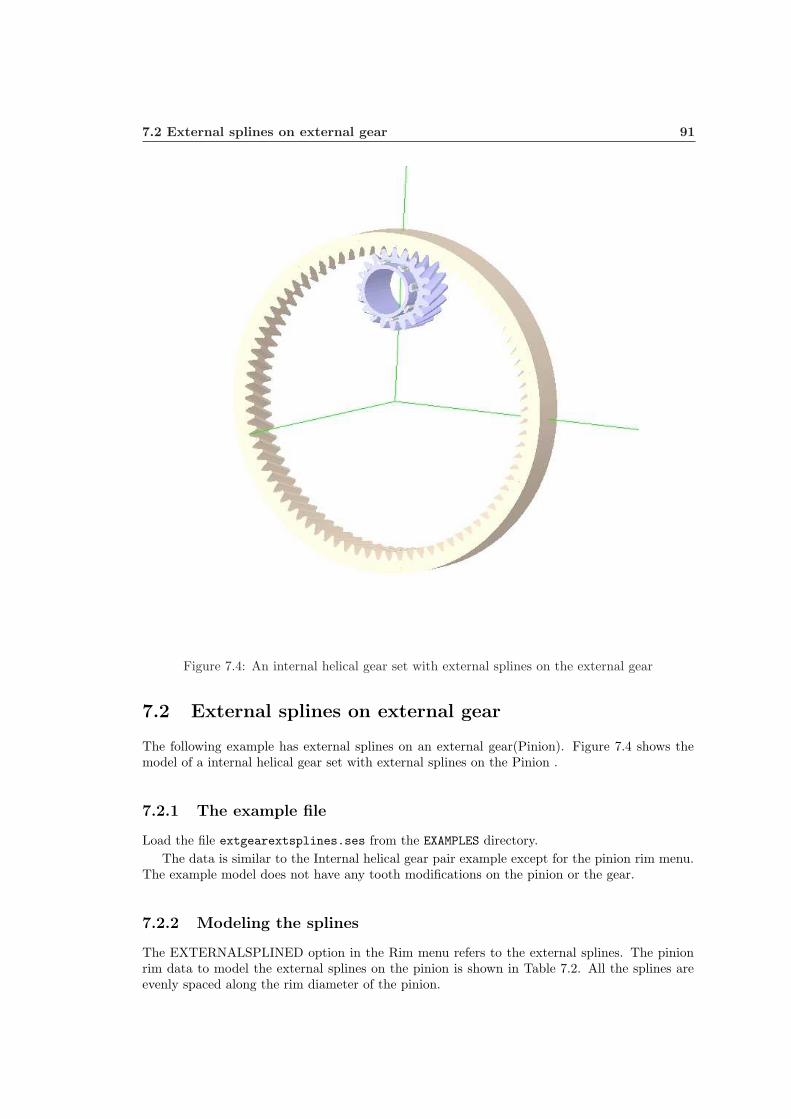
7.2 External splines on external gear 91
Figure 7.4: An internal helical gear set with external splines on the external gear
7.2 External splines on external gear
The following example has external splines on an external gear(Pinion). Figure 7.4 shows themodel of a internal helical gear set with external splines on the Pinion .
7.2.1 The example file
Load the file extgearextsplines.ses from the EXAMPLES directory.The data is similar to the Internal helical gear pair example except for the pinion rim menu.
The example model does not have any tooth modifications on the pinion or the gear.
7.2.2 Modeling the splines
The EXTERNALSPLINED option in the Rim menu refers to the external splines. The pinionrim data to model the external splines on the pinion is shown in Table 7.2. All the splines areevenly spaced along the rim diameter of the pinion.
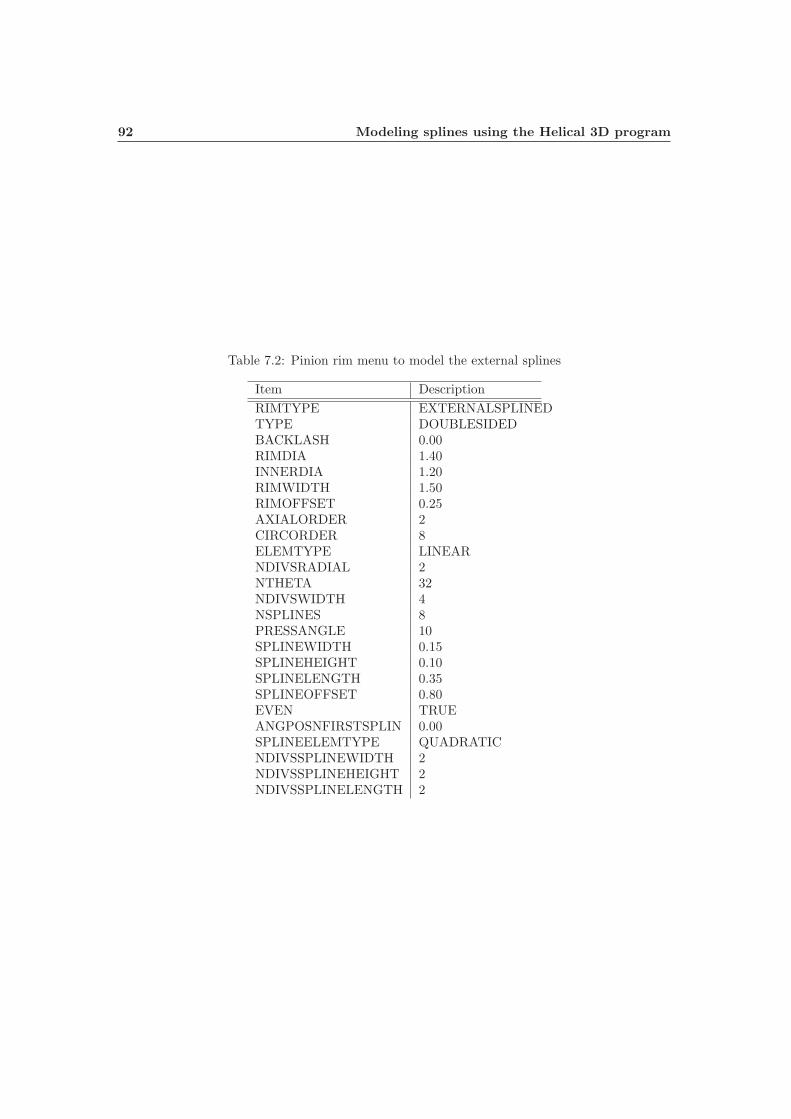
92 Modeling splines using the Helical 3D program
Table 7.2: Pinion rim menu to model the external splines
Item DescriptionRIMTYPE EXTERNALSPLINEDTYPE DOUBLESIDEDBACKLASH 0.00RIMDIA 1.40INNERDIA 1.20RIMWIDTH 1.50RIMOFFSET 0.25AXIALORDER 2CIRCORDER 8ELEMTYPE LINEARNDIVSRADIAL 2NTHETA 32NDIVSWIDTH 4NSPLINES 8PRESSANGLE 10SPLINEWIDTH 0.15SPLINEHEIGHT 0.10SPLINELENGTH 0.35SPLINEOFFSET 0.80EVEN TRUEANGPOSNFIRSTSPLIN 0.00SPLINEELEMTYPE QUADRATICNDIVSSPLINEWIDTH 2NDIVSSPLINEHEIGHT 2NDIVSSPLINELENGTH 2

7.2 External splines on external gear 93
Figure 7.5: Maximum principal normal stress contour for an internal helical gear set with externalsplines on the pinion
7.2.3 Results
After the analysis is complete a postprocessing file is created in the working directory. Figure 7.5shows the maximum principal normal stress contour for the internal helical gear pair. Figure 7.6shows the load distribution on the pinion and the splines.

94 Modeling splines using the Helical 3D program
Figure 7.6: Load distribution on the pinion and the splines
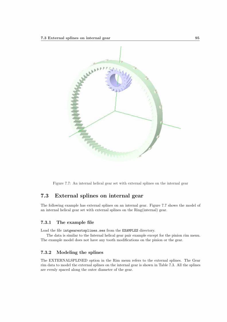
7.3 External splines on internal gear 95
Figure 7.7: An internal helical gear set with external splines on the internal gear
7.3 External splines on internal gear
The following example has external splines on an internal gear. Figure 7.7 shows the model ofan internal helical gear set with external splines on the Ring(internal) gear.
7.3.1 The example file
Load the file intgearextsplines.ses from the EXAMPLES directory.The data is similar to the Internal helical gear pair example except for the pinion rim menu.
The example model does not have any tooth modifications on the pinion or the gear.
7.3.2 Modeling the splines
The EXTERNALSPLINED option in the Rim menu refers to the external splines. The Gearrim data to model the external splines on the internal gear is shown in Table 7.3. All the splinesare evenly spaced along the outer diameter of the gear.

96 Modeling splines using the Helical 3D program
Table 7.3: Gear rim menu to model the external splines
Item DescriptionRIMTYPE EXTERNALSPLINEDTYPE DOUBLESIDEDBACKLASH 0.00RIMDIA 8.65OUTERDIA 9.00RIMWIDTH 1.00RIMOFFSET 0.00AXIALORDER 2CIRCORDER 16ELEMTYPE QUADRATICNDIVSRADIAL 4NTHETA 64NDIVSWIDTH 4NSPLINES 20PRESSANGLE 25SPLINEWIDTH 0.20SPLINEHEIGHT 0.10SPLINELENGTH 0.30SPLINEOFFSET -0.25EVEN TRUEANGPOSNFIRSTSPLIN 0.00SPLINEELEMTYPE QUADRATICNDIVSSPLINEWIDTH 2NDIVSSPLINEHEIGHT 2NDIVSSPLINELENGTH 2

7.3 External splines on internal gear 97
Figure 7.8: Maximum principal normal stress contour for an internal helical gear set with externalsplines on the internal gear
7.3.3 Results
After the analysis is complete a postprocessing file is created in the working directory. Figure 7.8shows the maximum principal normal stress contour for the internal helical gear pair. Figure 7.9shows the contact pressure distribution on the gear and the splines.

98 Modeling splines using the Helical 3D program
Figure 7.9: Contact pressure distribution for an internal helical gear set with external splines onthe internal gear

7.4 Internal splines on internal gear 99
Figure 7.10: An internal helical gear set with internal splines on the internal gear
7.4 Internal splines on internal gear
The following example has internal splines on an internal gear. Figure 7.10 shows the model ofan internal helical gear set with internal splines on the Ring(internal) gear.
7.4.1 The example file
Load the file intgearintsplines.ses from the EXAMPLES directory.The data is similar to the Internal helical gear pair example except for the gear rim menu.
The example model does not have any tooth modifications on the pinion or the gear.
7.4.2 Modeling the splines
The INTERNALSPLINED option in the Rim menu refers to the internal splines. The Gear rimdata to model the internal splines on the internal gear is shown in Table 7.4. All the splines areevenly spaced along the rim diameter of the gear.

100 Modeling splines using the Helical 3D program
Table 7.4: Gear rim menu to model the internal splines
Item DescriptionRIMTYPE INTERNALSPLINEDTYPE DOUBLESIDEDBACKLASH 0.00RIMDIA 8.65OUTERDIA 9.00RIMWIDTH 1.50RIMOFFSET 0.25AXIALORDER 2CIRCORDER 16ELEMTYPE QUADRATICNDIVSRADIAL 4NTHETA 64NDIVSWIDTH 4NSPLINES 20PRESSANGLE 25SPLINEWIDTH 0.20SPLINEHEIGHT 0.10SPLINELENGTH 0.30SPLINEOFFSET 0.85EVEN TRUEANGPOSNFIRSTSPLIN 0.00SPLINEELEMTYPE QUADRATICNDIVSSPLINEWIDTH 2NDIVSSPLINEHEIGHT 2NDIVSSPLINELENGTH 2
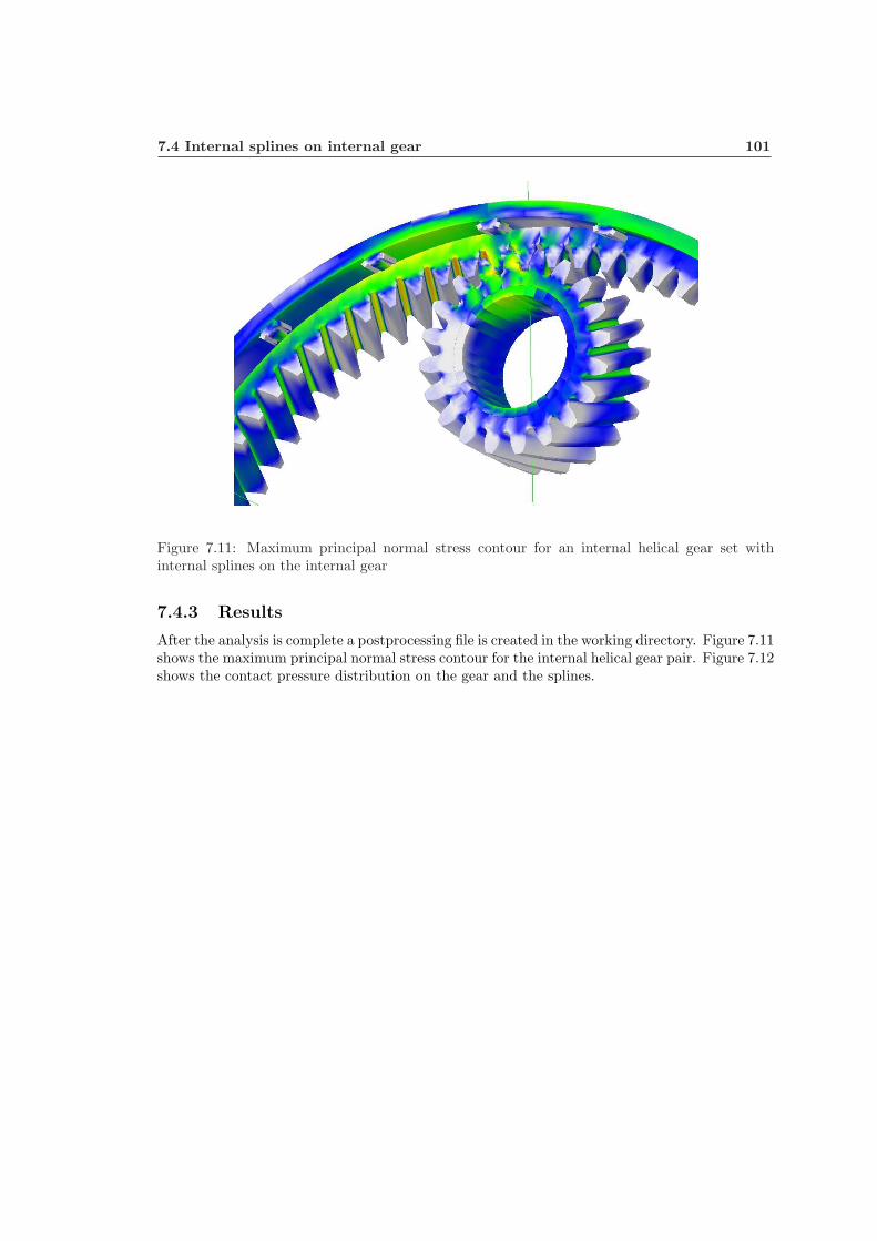
7.4 Internal splines on internal gear 101
Figure 7.11: Maximum principal normal stress contour for an internal helical gear set withinternal splines on the internal gear
7.4.3 Results
After the analysis is complete a postprocessing file is created in the working directory. Figure 7.11shows the maximum principal normal stress contour for the internal helical gear pair. Figure 7.12shows the contact pressure distribution on the gear and the splines.

102 Modeling splines using the Helical 3D program
Figure 7.12: Contact pressure distribution for an internal helical gear set with internal splineson the internal gear
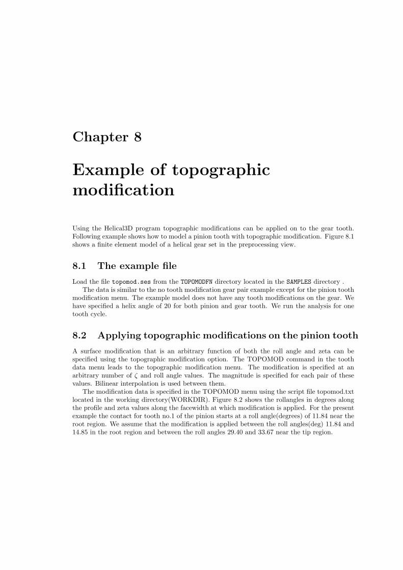
Chapter 8
Example of topographicmodification
Using the Helical3D program topographic modifications can be applied on to the gear tooth.Following example shows how to model a pinion tooth with topographic modification. Figure 8.1shows a finite element model of a helical gear set in the preprocessing view.
8.1 The example file
Load the file topomod.ses from the TOPOMODFN directory located in the SAMPLES directory .The data is similar to the no tooth modification gear pair example except for the pinion tooth
modification menu. The example model does not have any tooth modifications on the gear. Wehave specified a helix angle of 20 for both pinion and gear tooth. We run the analysis for onetooth cycle.
8.2 Applying topographic modifications on the pinion tooth
A surface modification that is an arbitrary function of both the roll angle and zeta can bespecified using the topographic modification option. The TOPOMOD command in the toothdata menu leads to the topographic modification menu. The modification is specified at anarbitrary number of ζ and roll angle values. The magnitude is specified for each pair of thesevalues. Bilinear interpolation is used between them.
The modification data is specified in the TOPOMOD menu using the script file topomod.txtlocated in the working directory(WORKDIR). Figure 8.2 shows the rollangles in degrees alongthe profile and zeta values along the facewidth at which modification is applied. For the presentexample the contact for tooth no.1 of the pinion starts at a roll angle(degrees) of 11.84 near theroot region. We assume that the modification is applied between the roll angles(deg) 11.84 and14.85 in the root region and between the roll angles 29.40 and 33.67 near the tip region.
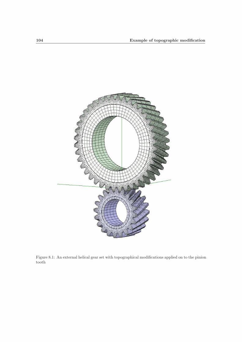
104 Example of topographic modification
Figure 8.1: An external helical gear set with topographical modifications applied on to the piniontooth
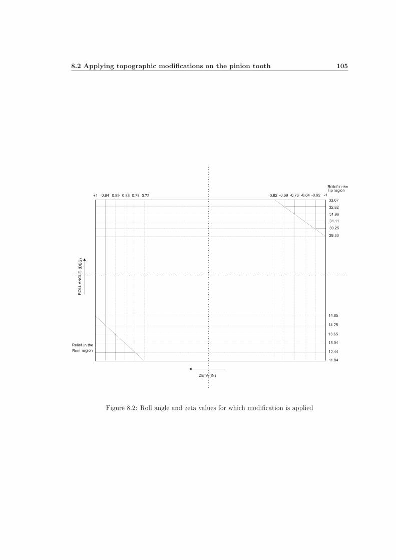
8.2 Applying topographic modifications on the pinion tooth 105
Figure 8.2: Roll angle and zeta values for which modification is applied

106 Example of topographic modification
The zeta extension for modification is found using the following:
From the Pinion tooth geometry data:
Pitch diam(Dp) = 2in
Helix angle(ψ) = 20o
Facewidth(W ) = 1in
Lead(L) =πDp
tanψ
= 17.2629in
In the root region :
Distance of modfn along the profile in roll angle(θ) = 14.85− 11.84= 3.01o
Distance of modification along the profile in inches = rb × θ(rads)= 0.9395× 0.0525= 0.049in
Distance of modification along the width in inches =0.049× L
2π= 0.135in.
Note that the ZETA along the facewidth goes from -1 to +1.
The corresponding Zeta distance of modification along the facewidth is 0.135 × 2 = 0.27in.
In the tip region :
Distance of modfn along the profile in roll angle(θ) = 33.67− 29.40= 4.27o
Distance of modification along the profile in inches = rb × θ(rads)= 0.9395× 0.0745= 0.07in
Distance of modification along the width in inches =0.07× L
2π= 0.192in.
The corresponding Zeta distance of modification along the facewidth is 0.192 × 2 = 0.384in.

8.3 Results 107
For this example we have considered 6 points along the modified profile and width in both theroot and the tip region as shown in Figure 8.2. In the root region, maximum modification mag-nitude of 0.0005in is applied at Rollangle(deg) and zeta(in) value of 11.84 and +1 respectively.In the tip region, maximum modification magnitude of 0.0005in is applied at Rollangle(deg) andzeta(in) value of 33.67 and −1 respectively. We reduce the modification magnitude in steps of0.0001in as we go away from the root and the tip regions. The modification at roll angles(deg)14.85 and 29.30 is 0.00in. Refer to the text file topomod.txt for further details.
8.3 Results
After the analysis is complete a postprocessing file is created in the working directory. Figure 8.3shows the contact pattern plot for pinion tooth with topographical modification. The relievedtip region at Zeta = −1 and root region at Zeta = 1 can be clearly seen in this plot. Figure 8.4shows the contact pattern plot for pinion tooth without any modifications. Figure 8.5 shows thebody deflection plot for pinion tooth with topographical modification. The transmission errorfor the gear model with modification is 1.953× 10⁻⁵rads = 1.8348× 10⁻⁵in. Figure 8.6 showsthe body deflection plot for pinion tooth without any modifications. The transmission error forthe Helical gear set without any modification is 2.508× 10⁻⁵rads = 2.356× 10⁻⁵in.

108 Example of topographic modification
Z
R
Con
tact
Pre
ssur
e
0.00
0E+
000
1.25
0E+
004
2.50
0E+
004
3.75
0E+
004
5.00
0E+
004
7.50
0E+
004
1.00
0E+
005
1.50
0E+
005
2.00
0E+
005
Figure 8.3: Contact pattern for pinion tooth with topographical modifications

8.3 Results 109
Z
R
Con
tact
Pre
ssur
e
0.00
0E+
000
1.25
0E+
004
2.50
0E+
004
3.75
0E+
004
5.00
0E+
004
7.50
0E+
004
1.00
0E+
005
1.50
0E+
005
2.00
0E+
005
Figure 8.4: Contact pattern for pinion tooth without any modifications

110 Example of topographic modification
-0.6
0000
0-0
.400
000
-0.2
0000
0-0
.000
000
0.20
0000
0.40
0000
0.60
0000
-0.0
0073
8
-0.0
0073
6
-0.0
0073
4
-0.0
0073
2
-0.0
0073
0
-0.0
0072
8
-0.0
0072
6
-0.0
0072
4
-0.0
0072
2
-0.0
0072
0
-0.0
0071
8
-0.0
0071
6
-0.0
0071
4
Tim
e
Bod
y Fr
ame
defl
ectio
n T
HE
TA
Z
TH
ET
AZ
, Ran
ge=
[-7.
3736
50E
-004
,-7.
1782
90E
-004
], P
eak
to P
eak=
1.95
3600
E-0
05
Figure 8.5: Body deflection plot showing the transmission error for pinion tooth with topograph-ical modifications
8.3 Results 111
-0.6
0000
0-0
.400
000
-0.2
0000
0-0
.000
000
0.20
0000
0.40
0000
0.60
0000
-0.0
0072
0
-0.0
0071
0
-0.0
0070
0
-0.0
0069
0
-0.0
0068
0
Tim
e
Bod
y Fr
ame
defl
ectio
n T
HE
TA
Z
TH
ET
AZ
, Ran
ge=
[-7.
1826
90E
-004
,-6.
9318
90E
-004
], P
eak
to P
eak=
2.50
8000
E-0
05
Figure 8.6: Body deflection plot showing the transmission error for pinion tooth without anymodifications

112 Example of topographic modification
Chapter 9
Convergence study
The following test cases are meant to study the effect of various parameters such as tip radius,thickness, nfaceelems and displorder on the maximum principle normal stress for a helical pinionand also the convergence of the stress values for different types of mesh templates.
9.1 Effect of Tip radius on the max ppl normal stress
9.1.1 The example file
Load the file convergence.ses from the CONVERGENCE directory located in the SAMPLES directory.Tables 9.1 through 9.10 show the data to be entered in the EDIT menu for running the
analysis. No assembly errors are considered for the pinion and the gear. Also there are nobearings in the model. In order to study the effect of tip radius on the stress values we run theanalysis for different tip radii for all the mesh templates. We vary the tip radius from 0.01in to0.045in in steps of 0.005in.

114 Convergence study
Table 9.1: System configuration parameters
Item DescriptionMESHTYPE CALYX3DCENTERDIST 3.00OFFSET 0.00ROTX 0.00ROTY 0.00INPUT PINIONTORQUEINPUT 1000.00RPMINPUT -3.00MU 0.00MAGRUNOUTGEAR 0.00ANGRUNOUTGEAR 0.00MAGRUNOUTPINION 0.00ANGRUNOUTPINION 0.00BACKSIDECONTACT FALSE
Table 9.2: Pinion data
Item DescriptionLUMPMASS 0.00LUMPMOMINERTIA 0.00LUMPALPHA 0.00
Table 9.3: Pinion tooth data
Item DescriptionNTEETH 20NFACEELEMS 4COORDORDER 10DISPLORDER 3PLANE TRANSVERSEXVERSEDIAMPITCH 10XVERSEPRESSANGLE 20XVERSETHICK 0.15708FACEWIDTH 1HAND LEFTHELIXANGLE 0.00RACKTIPRAD 0.02OUTERDIA 2.18ROOTDIA 1.76RIMDIA 1.40YOUNGSMOD 3x10⁷
POISSON 0.3MSHFILE pinion.mshTPLFILE medium.tpl

9.1 Effect of Tip radius on the max ppl normal stress 115
Table 9.4: Modification menu for the pinion tooth
Item DescriptionQUADTIPMOD TRUEROLLQUADTIPMOD 27.25MAGQUADTIPMOD 0.0005LEADCROWN 0.0005
Table 9.5: Pinion rim data
Item DescriptionRIMTYPE SIMPLERIMDIA 1.40INNERDIA 1.20WIDTH 1.00OFFSET 0.00AXIALORDER 2CIRCORDER 8ELEMTYPE LINEARNDIVSRADIAL 2NTHETA 32NDIVSWIDTH 4
Table 9.6: Gear data
Item DescriptionTYPE EXTERNALLUMPMASS 0.00LUMPMOMINERTIA 0.00LUMPALPHA 0.00
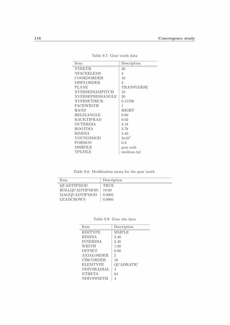
116 Convergence study
Table 9.7: Gear tooth data
Item DescriptionNTEETH 40NFACEELEMS 4COORDORDER 10DISPLORDER 3PLANE TRANSVERSEXVERSEDIAMPITCH 10XVERSEPRESSANGLE 20XVERSETHICK 0.15708FACEWIDTH 1HAND RIGHTHELIXANGLE 0.00RACKTIPRAD 0.02OUTERDIA 4.18ROOTDIA 3.78RIMDIA 3.40YOUNGSMOD 3x10⁷
POISSON 0.3MSHFILE gear.mshTPLFILE medium.tpl
Table 9.8: Modification menu for the gear tooth
Item DescriptionQUADTIPMOD TRUEROLLQUADTIPMOD 19.60MAGQUADTIPMOD 0.0005LEADCROWN 0.0005
Table 9.9: Gear rim data
Item DescriptionRIMTYPE SIMPLERIMDIA 3.40INNERDIA 2.40WIDTH 1.00OFFSET 0.00AXIALORDER 2CIRCORDER 16ELEMTYPE QUADRATICNDIVSRADIAL 4NTHETA 64NDIVSWIDTH 4

9.1 Effect of Tip radius on the max ppl normal stress 117
Table 9.10: Setup data
Item DescriptionSEPTOL 0.01NPROFDIVS 8NFACEDIVS 12DSPROF 0.001ZEROINITIAL TRUEINITIALTIME 0.0NRANGES 1RANGE 1SOLMETHOD STATICNTIMESTEPS 11DELTATIME 0.1STARTSPEEDFACTOR 1.0STARTTORQUEFACTOR 1.0ENDTORQUEFACTOR 1.0SAVEPERIODICALLY FALSEOUTPUTRESTART FALSEPOSTPROCWRITE TRUEPOSTFILENAME postproc.datNSTEPSWRITE 1
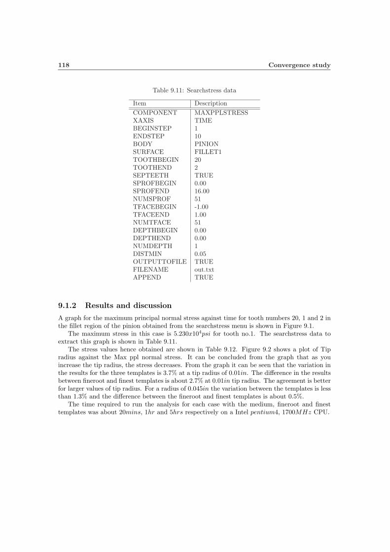
118 Convergence study
Table 9.11: Searchstress data
Item DescriptionCOMPONENT MAXPPLSTRESSXAXIS TIMEBEGINSTEP 1ENDSTEP 10BODY PINIONSURFACE FILLET1TOOTHBEGIN 20TOOTHEND 2SEPTEETH TRUESPROFBEGIN 0.00SPROFEND 16.00NUMSPROF 51TFACEBEGIN -1.00TFACEEND 1.00NUMTFACE 51DEPTHBEGIN 0.00DEPTHEND 0.00NUMDEPTH 1DISTMIN 0.05OUTPUTTOFILE TRUEFILENAME out.txtAPPEND TRUE
9.1.2 Results and discussion
A graph for the maximum principal normal stress against time for tooth numbers 20, 1 and 2 inthe fillet region of the pinion obtained from the searchstress menu is shown in Figure 9.1.
The maximum stress in this case is 5.230x10⁴psi for tooth no.1. The searchstress data toextract this graph is shown in Table 9.11.
The stress values hence obtained are shown in Table 9.12. Figure 9.2 shows a plot of Tipradius against the Max ppl normal stress. It can be concluded from the graph that as youincrease the tip radius, the stress decreases. From the graph it can be seen that the variation inthe results for the three templates is 3.7% at a tip radius of 0.01in. The difference in the resultsbetween fineroot and finest templates is about 2.7% at 0.01in tip radius. The agreement is betterfor larger values of tip radius. For a radius of 0.045in the variation between the templates is lessthan 1.3% and the difference between the fineroot and finest templates is about 0.5%.
The time required to run the analysis for each case with the medium, fineroot and finesttemplates was about 20mins, 1hr and 5hrs respectively on a Intel pentium4, 1700MHz CPU.
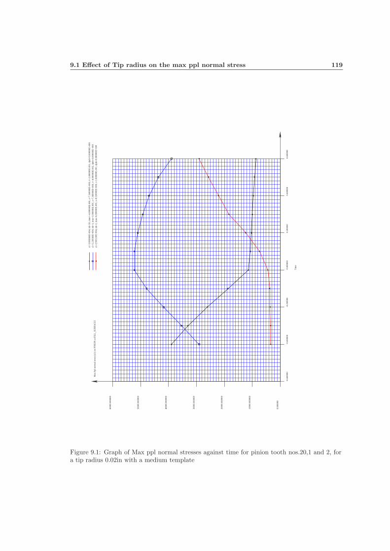
9.1 Effect of Tip radius on the max ppl normal stress 119
-0.6
0000
0-0
.400
000
-0.2
0000
0-0
.000
000
0.20
0000
0.40
0000
0.60
0000
0.00
0000
1000
0.00
0000
2000
0.00
0000
3000
0.00
0000
4000
0.00
0000
5000
0.00
0000
6000
0.00
0000
Tim
e
Max
Ppl
nor
mal
str
ess
(s1)
on
PIN
ION
at F
ILL
_SU
RFA
CE
1
s1=
3.89
3800
E+
004,
tth=
20, t
ime=
-4.0
0000
0E-0
01, s
=7.
3600
00E
+00
0, t=
-2.8
0000
0E-0
01, d
pth=
0.00
0000
E+
000
s1=
5.23
0360
E+
004,
tth=
1, ti
me=
1.00
0000
E-0
01, s
=7.
3600
00E
+00
0, t=
-4.0
0000
0E-0
02, d
pth=
0.00
0000
E+
000
s1=
2.90
5130
E+
004,
tth=
2, ti
me=
6.00
0000
E-0
01, s
=8.
3200
00E
+00
0, t=
1.60
0000
E-0
01, d
pth=
0.00
0000
E+
000
Figure 9.1: Graph of Max ppl normal stresses against time for pinion tooth nos.20,1 and 2, fora tip radius 0.02in with a medium template
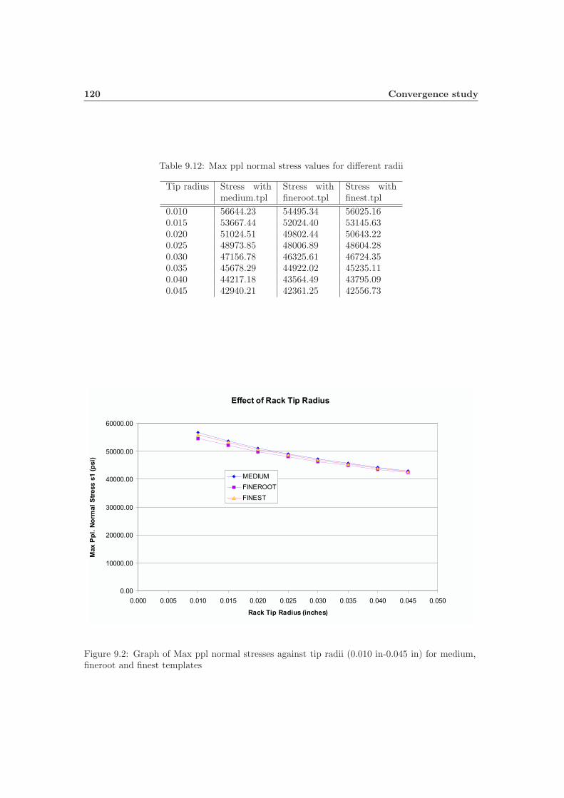
120 Convergence study
Table 9.12: Max ppl normal stress values for different radii
Tip radius Stress withmedium.tpl
Stress withfineroot.tpl
Stress withfinest.tpl
0.010 56644.23 54495.34 56025.160.015 53667.44 52024.40 53145.630.020 51024.51 49802.44 50643.220.025 48973.85 48006.89 48604.280.030 47156.78 46325.61 46724.350.035 45678.29 44922.02 45235.110.040 44217.18 43564.49 43795.090.045 42940.21 42361.25 42556.73
Effect of Rack Tip Radius
0.00
10000.00
20000.00
30000.00
40000.00
50000.00
60000.00
0.000 0.005 0.010 0.015 0.020 0.025 0.030 0.035 0.040 0.045 0.050
Rack Tip Radius (inches)
Max
Pp
l.N
orm
al
Str
ess
s1
(psi)
MEDIUM
FINEROOT
FINEST
Figure 9.2: Graph of Max ppl normal stresses against tip radii (0.010 in-0.045 in) for medium,fineroot and finest templates
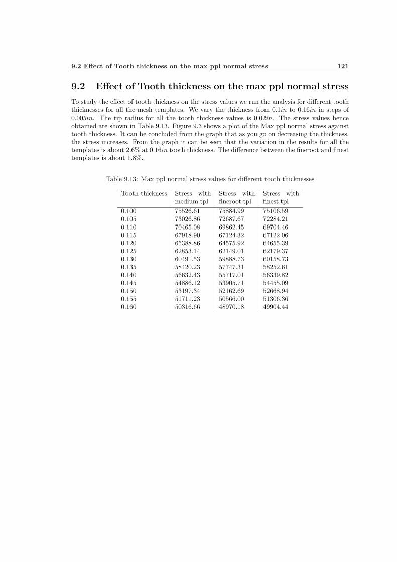
9.2 Effect of Tooth thickness on the max ppl normal stress 121
9.2 Effect of Tooth thickness on the max ppl normal stress
To study the effect of tooth thickness on the stress values we run the analysis for different tooththicknesses for all the mesh templates. We vary the thickness from 0.1in to 0.16in in steps of0.005in. The tip radius for all the tooth thickness values is 0.02in. The stress values henceobtained are shown in Table 9.13. Figure 9.3 shows a plot of the Max ppl normal stress againsttooth thickness. It can be concluded from the graph that as you go on decreasing the thickness,the stress increases. From the graph it can be seen that the variation in the results for all thetemplates is about 2.6% at 0.16in tooth thickness. The difference between the fineroot and finesttemplates is about 1.8%.
Table 9.13: Max ppl normal stress values for different tooth thicknesses
Tooth thickness Stress withmedium.tpl
Stress withfineroot.tpl
Stress withfinest.tpl
0.100 75526.61 75884.99 75106.590.105 73026.86 72687.67 72284.210.110 70465.08 69862.45 69704.460.115 67918.90 67124.32 67122.060.120 65388.86 64575.92 64655.390.125 62853.14 62149.01 62179.370.130 60491.53 59888.73 60158.730.135 58420.23 57747.31 58252.610.140 56632.43 55717.01 56339.820.145 54886.12 53905.71 54455.090.150 53197.34 52162.69 52668.940.155 51711.23 50566.00 51306.360.160 50316.66 48970.18 49904.44

122 Convergence study
Effect of Tooth Thickness
0.00
10000.00
20000.00
30000.00
40000.00
50000.00
60000.00
70000.00
80000.00
0.080 0.090 0.100 0.110 0.120 0.130 0.140 0.150 0.160 0.170
Transverse Circular Tooth Thickness (inches)
Max
Pp
l.N
orm
al
Str
ess
s1
(psi)
MEDIUM
FINEROOT
FINEST
Figure 9.3: Graph of Max ppl normal stresses against tooth thickness (0.10in-0.16in) for medium,fineroot and finest templates

9.3 Effect of number of elements in the face direction on the max ppl normal stress123
9.3 Effect of number of elements in the face direction onthe max ppl normal stress
To study the effect of number of elements along the face width on the stress values we run theanalysis for different NFACEELEMS for all the mesh templates. The polynomial order of theelements DISPLORDER is maintained at 3. We vary the NFACEELEMS parameter from 2 to10 in steps of 2. The tip radius and the tooth thickness values for all the test cases are 0.02inand 0.15708in respectively. The stress values hence obtained are shown in Table 9.14. Figure 9.4shows a plot of the Max ppl normal stress against the no. of face elements for the medium andfineroot templates. Results for higher elements with the finest mesh could not be obtained dueto CPU limitations. As expected the stress values converge for higher number of elements. Forthe fineroot template, the difference between 2 elements and 10 elements is less than 0.1%. Thisimplies that the stress variation in the face direction in the fillet can be well approximated evenwith 4 elements when a polynomial order of 3 is used along the face width.
Table 9.14: Max ppl normal stress values for different number of elements along the face width
Nfaceelems Stress withmedium.tpl
Stress withfineroot.tpl
Stress withfinest.tpl
2 51107.14 49911.72 50799.474 51024.51 49802.44 50643.226 51084.53 49867.04 -8 51082.93 49865.59 -10 51079.74 49862.72 -
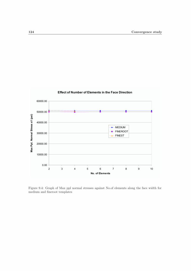
124 Convergence study
Effect of Number of Elements in the Face Direction
0.00
10000.00
20000.00
30000.00
40000.00
50000.00
60000.00
2 3 4 5 6 7 8 9 10
No. of Elements
Max
Pp
l.N
orm
al
Str
ess
s1
(psi)
MEDIUM
FINEROOT
FINEST
Figure 9.4: Graph of Max ppl normal stresses against No.of elements along the face width formedium and fineroot templates
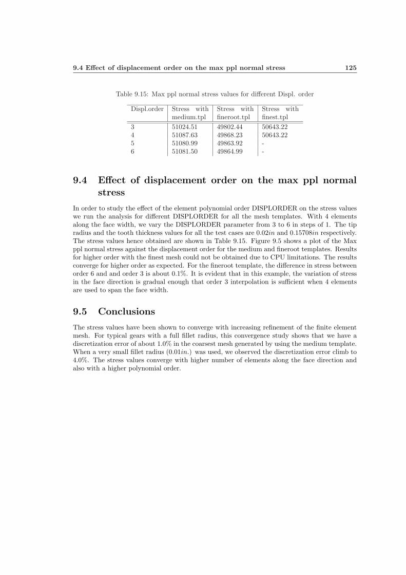
9.4 Effect of displacement order on the max ppl normal stress 125
Table 9.15: Max ppl normal stress values for different Displ. order
Displ.order Stress withmedium.tpl
Stress withfineroot.tpl
Stress withfinest.tpl
3 51024.51 49802.44 50643.224 51087.63 49868.23 50643.225 51080.99 49863.92 -6 51081.50 49864.99 -
9.4 Effect of displacement order on the max ppl normalstress
In order to study the effect of the element polynomial order DISPLORDER on the stress valueswe run the analysis for different DISPLORDER for all the mesh templates. With 4 elementsalong the face width, we vary the DISPLORDER parameter from 3 to 6 in steps of 1. The tipradius and the tooth thickness values for all the test cases are 0.02in and 0.15708in respectively.The stress values hence obtained are shown in Table 9.15. Figure 9.5 shows a plot of the Maxppl normal stress against the displacement order for the medium and fineroot templates. Resultsfor higher order with the finest mesh could not be obtained due to CPU limitations. The resultsconverge for higher order as expected. For the fineroot template, the difference in stress betweenorder 6 and and order 3 is about 0.1%. It is evident that in this example, the variation of stressin the face direction is gradual enough that order 3 interpolation is sufficient when 4 elementsare used to span the face width.
9.5 Conclusions
The stress values have been shown to converge with increasing refinement of the finite elementmesh. For typical gears with a full fillet radius, this convergence study shows that we have adiscretization error of about 1.0% in the coarsest mesh generated by using the medium template.When a very small fillet radius (0.01in.) was used, we observed the discretization error climb to4.0%. The stress values converge with higher number of elements along the face direction andalso with a higher polynomial order.

126 Convergence study
Effect of Displacement Order
0.00
10000.00
20000.00
30000.00
40000.00
50000.00
60000.00
3 4 5 6
Element Displacement Order
Max
Pp
l.N
orm
al
Str
ess
s1
(psi)
MEDIUM
FINEROOT
FINEST
Figure 9.5: Graph of Max ppl normal stresses against displacement order for medium and fineroottemplates

Chapter 10
Fatigue theory and life predictionusing the Helical gear program
10.1 Introduction
Most engineering design projects involve machine parts subjected to fluctuating or cyclic loads.Such loading induces fluctuating or cyclic stresses that often result in failure by fatigue. Materialsfracturing under repeated loadings were found to exhibit no gross deformation and gave theappearance of having suddenly snapped. It is difficult to detect the progressive changes in thematerial properties that occur during fatigue stressing and failure may therefore occur withlittle or no warning. Also, periods of rest, with the fatigue stress removed, do not lead to anymeasurable healing or recovery from the effects of prior cyclic stressing. Thus the damage doneduring the fatigue process is cumulative and generally unrecoverable.
With the increasing demand for more efficient and economic components and structuresoperation at higher speeds with minimum weight design the number of failures by fatigue hascontinued to increase. It is by far the most common cause of failure of load carrying metallicparts operating at or close to room temperature.
10.2 Fatigue characteristics
Fatigue may be characterised as a progressive failure phenomenon that proceeds by the initiationand propagation of cracks to an unstable size. Fatigue crack nuclei, from which crack grows andoften propagate to failure, are thought to be formed through the movements of dislocationsthat produce fine slip bands at the crystal surfaces. Under cyclic loading these fine slip bandsultimately turn out to be the regions in which fatigue cracks are initiated. Further, the fatigueslip bands gives rise to intrusions as a result of reversed slip in adjacent slip planes caused byload reversal. Once formed, these intrusions grow in depth by reverse slip process, and theirgrowth may well constitute a major portion of the fatigue of the metal. Crack propagation andhence fatigue are affected by various factors such as material composition, grain size and graindirection, heat treatment, welding, geometrical discontinuities, surface conditions, size, residualsurface stresses, corrosion, fretting, operating temperature, operating speed, etc.
A term called fatigue limit(endurance limit) is very commonly used while studying fatiguefailure. It is the stress level below which an infinite number of cycles can be sustained withoutfailure. To characterize the failure response of components in the finite life range, the termfatigue strength at a specified life, SN is used. The term fatigue strength identifies the stresslevel at which failure will occur at specified life.

128 Fatigue theory and life prediction using the Helical gear program
σmax
σmin
σm
= 0
Time
σa
∆σ
Str
ess
Figure 10.1: Completely reversed cyclic stress plot
10.3 Low and High cycle fatigue
It is observed that the fatigue process embraces two domains of cyclic stressing or straining thatare significantly different in character, and in each of which failure is probably produced bydifferent physical mechanisms. One domain of cyclic loading is that for which significant plasticstrains occur during each cycle. This domain is associated with high loads and short lives, or lownumber of cycles to produce fatigue failure, and is commonly referred to as low cycle fatigue.
The other domain of cyclic loading is that for which the strain cycles are largely confined tothe elastic range. This domain is associated with lower loads and long lives, or high number ofcycles to produce fatigue failure, and is commonly referred to as high cycle fatigue. Low-cyclefatigue is typically associated with cycle lives up to about 104 or 105 cycles, and high cyclefatigue for lives greater than about 104 or 105 cycles. In most gearing applications fatigue failureis associated with high cycle fatigue. Hence we address the helical fatigue failure problem basedon the theory related to the high cycle fatigue.
10.4 Fatigue loading
As discussed earlier fatigue failure is caused in materials or components when subjected to cyclicor alternating stress. A simple example of a fatigue stress spectrum to which an element may besubjected could be a zero-mean sinusoidal stress-time pattern of constant amplitude and fixedfrequency, applied for a specified number of cycles. Such a stress-time pattern, often referred toas a completely reversed cyclic stress is shown in Figure 10.1.
Using the figure we define the following terms and symbols so as to calculate the fatiguestrength or fatigue life for a helical gear set.

10.4 Fatigue loading 129
σmax
σmin
σm
Time
Str
ess
Figure 10.2: Nonzero mean stress-time pattern
σmax = Maximum Stress in the cycle (10.1)σmin = Minimum Stress in the cycle (10.2)
σm = Mean Stress
=σmax + σmin
2(10.3)
σa = Alternating Stress amplitude
=σmax − σmin
2(10.4)
∆σ = Range of Stress= σmax − σmin (10.5)
R = Stress Ratio
=σmin
σmax(10.6)
A = Amplitude Ratio
=σa
σm(10.7)
Some of the examples of Stress-time patterns are shown in Figures 10.2 through 10.7.
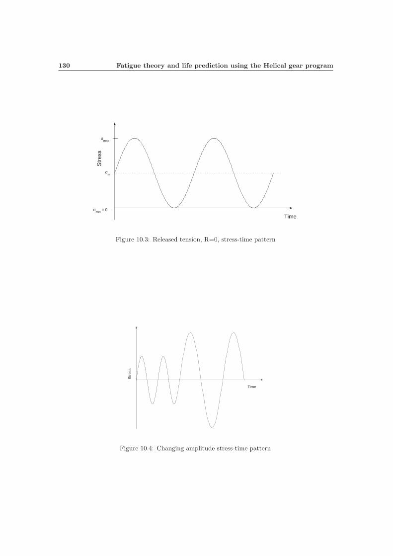
130 Fatigue theory and life prediction using the Helical gear program
σmax
σmin
= 0
σm
Time
Str
ess
Figure 10.3: Released tension, R=0, stress-time pattern
Str
ess
Time
Figure 10.4: Changing amplitude stress-time pattern

10.4 Fatigue loading 131
Figure 10.5: Quasi-random stress-time pattern
Figure 10.6: Completely reversed ramp stress-time pattern

132 Fatigue theory and life prediction using the Helical gear program
Figure 10.7: Stress-time pattern with distorted peaks

10.5 Example of a laboratory fatigue testing 133
10.5 Example of a laboratory fatigue testing
Designing machine parts or structures that are subjected to fatigue loading is usually based onthe results of laboratory fatigue tests using specimens of the material of interest. An exampleof a laboratory fatigue testing called as the rotating bending machine of the constant bendingmoment type is shown in Figure 10.8.
Figure 10.8: Schematic of the rotating-bending fatigue testing machine of the constant bendingmoment type
ω t
Str
ess
at A
Figure 10.9: Stress-time pattern for point A at the surface of the critical section

134 Fatigue theory and life prediction using the Helical gear program
With this type of device the region of the rotating beam between the inboard bearingsis subjected to a constant bending moment all along its length. While under the influenceof this constant moment, the specimen is caused to rotate with the drive spindles about thelongitudinal axis. Any point on the surface is thereby subjected to a completely reversed stress-time pattern, as can be deduced by following the stress history of a point as it rotates frommaximum compression at the top position down through zero stress when at the side throughmaximum tension at the bottom, and then back through zero to maximum compression at thetop again. The stress-time pattern for a point on the surface of the critical section is shown inFigure 10.9.
10.6 Gear fatigue failure
Gears may fail by wear and scuffing but the main causes of failure are bending fatigue leading tobreakage at the root of the tooth and surface contact fatigue leading to pitting. Fatigue failurein gears can be broadly classified in to two types:
• Those arising from a tensile fatigue failure of the material at the root of a gear tooth i.e.away from the area of contact between intermeshing teeth.
• Those arising from compressive stresses on the working surface of the gear tooth, whereit is in contact with the intermeshing gear.
Tensile fatigue failure occurs in materials subjected to fluctuating stresses where the continu-ously repeated stress is much lower than the static tensile strength of the material. This type ofhigh cycle fatigue failure generally depends upon the number of stress cycles rather than on thetotal time under load and does not occur below a certain stress, called the fatigue and endurancelimit. In a homogeneous material tensile fatigue crack always starts at and propagates from thepoint of maximum stress concentration. Under normal operation and with correct design thepoint of maximum tensile stress concentration on a gear is at the root of the tooth on the loadedside. The crack progresses through the tooth to the root on the opposite side. During thiscrack propagation the tooth can bend over and shed the load on to the next tooth which alsoultimately fails.
Surface fatigue failure is brought about by cumulative damage to the gear material caused byrepeated application of contact stresses. Surface contact fatigue does not usually lead to catas-trophic breakage (as in the case of a tensile fatigue failure) but rather to progressive deteriorationof the surface by pitting or spalling.
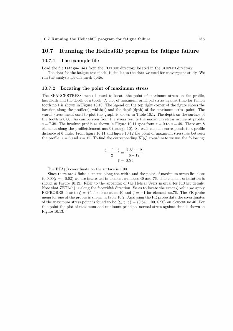
10.7 Running the Helical3D program for fatigue failure 135
10.7 Running the Helical3D program for fatigue failure
10.7.1 The example file
Load the file fatigue.ses from the FATIGUE directory located in the SAMPLES directory.The data for the fatigue test model is similar to the data we used for convergence study. We
run the analysis for one mesh cycle.
10.7.2 Locating the point of maximum stress
The SEARCHSTRESS menu is used to locate the point of maximum stress on the profile,facewidth and the depth of a tooth. A plot of maximum principal stress against time for Piniontooth no.1 is shown in Figure 10.10. The legend on the top right corner of the figure shows thelocation along the profile(s), width(t) and the depth(dpth) of the maximum stress point. Thesearch stress menu used to plot this graph is shown in Table 10.1. The depth on the surface ofthe tooth is 0.00. As can be seen from the stress results the maximum stress occurs at profile,s = 7.38. The involute profile as shown in Figure 10.11 goes from s = 0 to s = 48. There are 8elements along the profile(element nos.3 through 10). So each element corresponds to a profiledistance of 6 units. From figure 10.11 and figure 10.12 the point of maximum stress lies betweenthe profile, s = 6 and s = 12. To find the corresponding XI(ξ) co-ordinate we use the following:
ξ − (−1)2
=7.38− 126− 12
ξ = 0.54
The ETA(η) co-ordinate on the surface is 1.00.Since there are 4 finite elements along the width and the point of maximum stress lies close
to 0.00(t = −0.02) we are interested in element numbers 40 and 76. The element orientation isshown in Figure 10.12. Refer to the appendix of the Helical Users manual for further details.Note that ZETA(ζ) is along the facewidth direction. So as to locate the exact ζ value we applyFEPROBES close to ζ = +1 for element no.40 and ζ = −1 for element no.76. The FE probemenu for one of the probes is shown in table 10.2. Analysing the FE probe data the co-ordinatesof the maximum stress point is found to be (ξ, η, ζ) = (0.54, 1.00, 0.90) on element no.40. Forthis point the plot of maximum and minimum principal normal stress against time is shown inFigure 10.13.

136 Fatigue theory and life prediction using the Helical gear program
-0.6
0000
0-0
.400
000
-0.2
0000
0-0
.000
000
0.20
0000
0.40
0000
0.60
0000
2000
0.00
0000
3000
0.00
0000
4000
0.00
0000
5000
0.00
0000
6000
0.00
0000
Tim
e
Max
Ppl
nor
mal
str
ess
(s1)
on
PIN
ION
at F
ILL
_SU
RFA
CE
1
s1=
5.23
2980
E+
004,
tth=
1, ti
me=
1.00
0000
E-0
01, s
=7.
3880
00E
+00
0, t=
-2.0
0000
0E-0
02, d
pth=
0.00
0000
E+
000
Figure 10.10: Plot of maximum principal normal stress against time for pinion tooth no.1 usingthe SEARCHSTRESS menu

10.7 Running the Helical3D program for fatigue failure 137
Figure 10.11: The MEDIUM.TPL template file.

138 Fatigue theory and life prediction using the Helical gear program
Figure 10.12: Orientation of ξ, η and ζ on the tooth
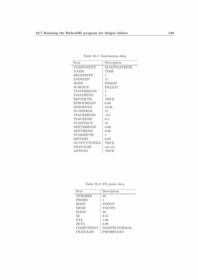
10.7 Running the Helical3D program for fatigue failure 139
Table 10.1: Searchstress data
Item DescriptionCOMPONENT MAXPPLSTRESSXAXIS TIMEBEGINSTEP 1ENDSTEP 11BODY PINIONSURFACE FILLET1TOOTHBEGIN 1TOOTHEND 1SEPTEETH TRUESPROFBEGIN 6.00SPROFEND 12.00NUMSPROF 51TFACEBEGIN -0.5TFACEEND 0.5NUMTFACE 51DEPTHBEGIN 0.00DEPTHEND 0.00NUMDEPTH 1DISTMIN 0.05OUTPUTTOFILE TRUEFILENAME out.txtAPPEND TRUE
Table 10.2: FE probe data
Item DescriptionNPROBES 40PROBE 1BODY PINIONMESH TOOTHELEM 40XI 0.54ETA 1.00ZETA 0.90COMPONENT MAXPPLNORMALFILENAME PROBES.DAT
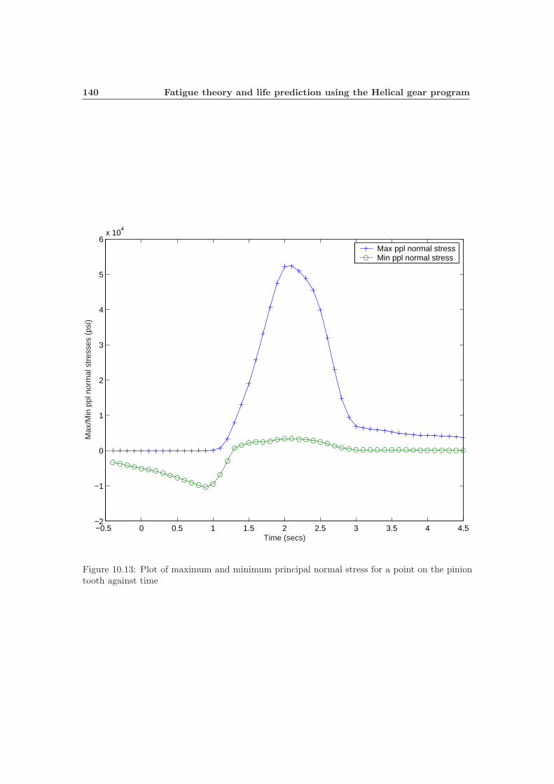
140 Fatigue theory and life prediction using the Helical gear program
−0.5 0 0.5 1 1.5 2 2.5 3 3.5 4 4.5−2
−1
0
1
2
3
4
5
6x 10
4
Time (secs)
Max
/Min
ppl
nor
mal
str
esse
s (p
si)
Max ppl normal stressMin ppl normal stress
Figure 10.13: Plot of maximum and minimum principal normal stress for a point on the piniontooth against time

10.7 Running the Helical3D program for fatigue failure 141
10.7.3 Results
The maximum principal and the minimum principal normal stress plot obtained from theFE probe data is shown in Figure 10.13. The maximum principal normal stress (σmax) =5.2330x10⁴psi and the minimum principal normal stress (σmin) = −9.7156x10³psi. Hence, Al-ternating stress, σa = 3.10232x10⁴psi and the Mean stress, σm = 2.13075x10⁴psi.

142 Fatigue theory and life prediction using the Helical gear program
Figure 10.14: An example of an S-N curve for predicting fatigue life
10.8 Calculating the fatigue life
The stress life, S-N, method was the first approach used in an attempt to understand and quantifyfatigue life. The S-N approach is still widely used in design applications where the applied stressis primarily within the elastic range of the material and the resultant lives (cycles to failures) arelong, such as power transmission shafts. The S-N diagram is a plot of alternating stress, S, versuscycles to failure, N. One of the major drawbacks of the stress-life approach is that it ignores thetrue stress-strain behavior and treats all strains as elastic. This may be significant since theinitiation of fatigue cracks is caused by plastic deformation. The simplifying assumptions of theS-N approach are valid only if the plastic strains are small. At long lives most steels have onlya small component of cyclic strain which is plastic and the S-N approach is valid. An exampleof an S-N plot is shown in Figure 10.14.
The magnitude of mean stress has an important influence on the fatigue behavior of a spec-imen or a machine part. Most service applications involve nonzero mean cyclic stresses. Thepresent case under consideration also is an example of a nonzero mean cyclic stress. The influ-ence of non-zero mean stress on failure can be estimated by empirical relationships (Figure 10.15)that relate the failure at a given life under non-zero mean conditions to failure at the same lifeunder zero mean cyclic stresses.

10.8 Calculating the fatigue life 143
Figure 10.15: Various empirical relationships for estimating the influence of nonzero-mean stresson fatigue failure
10.8.1 Goodman’s Linear relationship
Let,
σa = Alternating stress amplitudeσN = Fatigue strengthσm = Mean stressσu = Ultimate strength
σyp = Yield point stress
Goodman’s linear relationship states that fatigue failure occurs when
σa
σN+
σm
σu≥ 1 (10.8)
For G43400 steel 1 with tensile strength 140 kpsi and fatigue limit 71 kpsi, using the results forσa and σm, the Goodman linear relationship gives
σa
σN+
σm
σu= 0.5890

144 Fatigue theory and life prediction using the Helical gear program
10.8.2 Gerber’s parabolic relationship
Gerber’s parabolic relationship states that fatigue failure occurs when
σa
σN+ (
σm
σu)2 ≥ 1 (10.9)
For G43400 steel with tensile strength 140 kpsi and fatigue limit 71 kpsi, the Gerber’s parabolicrelationship gives
σa
σN+ (
σm
σu)2 = 0.4600
10.8.3 Soderberg’s linear relationship
Soderberg’s linear relationship states that fatigue failure occurs when
σa
σN+
σm
σyp
≥ 1 (10.10)
For G43400 steel with yield strength 100 kpsi and fatigue limit 71 kpsi, the Soderberg’s linearrelationship gives
σa
σN+
σm
σyp
= 0.6499
10.8.4 Elliptic relationship
Elliptic relationship states that fatigue failure occurs when
(σa
σN)2 + (
σm
σu)2 ≥ 1 (10.11)
For G43400 steel with tensile strength 140 kpsi and fatigue limit 71 kpsi, the Elliptic relationshipgives
(σa
σN)2 + (
σm
σu)2 = 0.2140
The above theories can be used to find the alternating stress at which fatigue failure will occur.For instance, according to the Goodman’s linear relationship, for a steel with tensile strength80 kpsi, the fatigue stress is 42.285 kpsi. Using an S-N plot for steel shown in Figure 10.16 2,the corresponding fatigue life is 4.5 × 10⁵ cycles. Note that the S-N plot used in the figure isnot a standard curve for gear materials. It is used to demonstrate the ability of the Helical3Dprogram in calculating the fatigue life.

10.8 Calculating the fatigue life 145
103
104
105
106
107
108
0.4
0.5
0.6
0.7
0.8
0.9
1
Life to failure, N(cycles)
Fat
igue
str
engt
h, S
e/U
ltim
ate
Str
engt
h, S
u
Figure 10.16: Example of an S-N plot for wrought steel
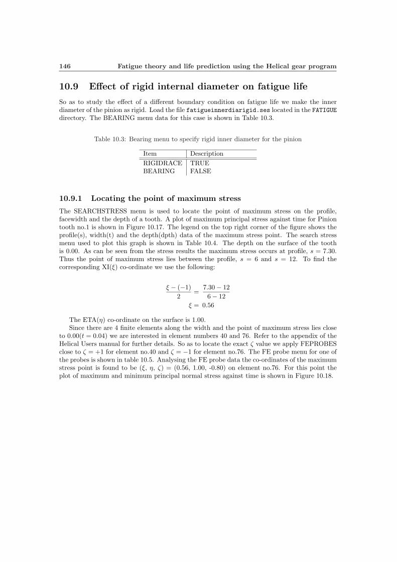
146 Fatigue theory and life prediction using the Helical gear program
10.9 Effect of rigid internal diameter on fatigue life
So as to study the effect of a different boundary condition on fatigue life we make the innerdiameter of the pinion as rigid. Load the file fatigueinnerdiarigid.ses located in the FATIGUEdirectory. The BEARING menu data for this case is shown in Table 10.3.
Table 10.3: Bearing menu to specify rigid inner diameter for the pinion
Item DescriptionRIGIDRACE TRUEBEARING FALSE
10.9.1 Locating the point of maximum stress
The SEARCHSTRESS menu is used to locate the point of maximum stress on the profile,facewidth and the depth of a tooth. A plot of maximum principal stress against time for Piniontooth no.1 is shown in Figure 10.17. The legend on the top right corner of the figure shows theprofile(s), width(t) and the depth(dpth) data of the maximum stress point. The search stressmenu used to plot this graph is shown in Table 10.4. The depth on the surface of the toothis 0.00. As can be seen from the stress results the maximum stress occurs at profile, s = 7.30.Thus the point of maximum stress lies between the profile, s = 6 and s = 12. To find thecorresponding XI(ξ) co-ordinate we use the following:
ξ − (−1)2
=7.30− 126− 12
ξ = 0.56
The ETA(η) co-ordinate on the surface is 1.00.Since there are 4 finite elements along the width and the point of maximum stress lies close
to 0.00(t = 0.04) we are interested in element numbers 40 and 76. Refer to the appendix of theHelical Users manual for further details. So as to locate the exact ζ value we apply FEPROBESclose to ζ = +1 for element no.40 and ζ = −1 for element no.76. The FE probe menu for one ofthe probes is shown in table 10.5. Analysing the FE probe data the co-ordinates of the maximumstress point is found to be (ξ, η, ζ) = (0.56, 1.00, -0.80) on element no.76. For this point theplot of maximum and minimum principal normal stress against time is shown in Figure 10.18.
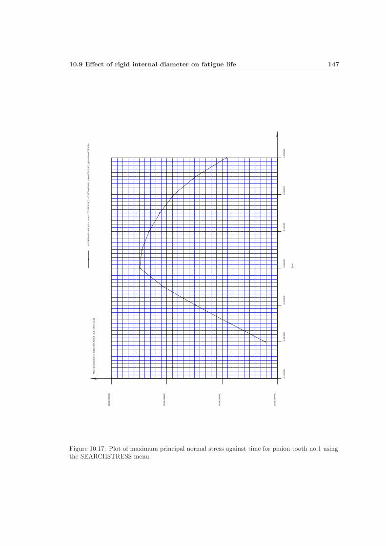
10.9 Effect of rigid internal diameter on fatigue life 147
-0.6
0000
0-0
.400
000
-0.2
0000
0-0
.000
000
0.20
0000
0.40
0000
0.60
0000
3000
0.00
0000
4000
0.00
0000
5000
0.00
0000
6000
0.00
0000
Tim
e
Max
Ppl
nor
mal
str
ess
(s1)
on
PIN
ION
at F
ILL
_SU
RFA
CE
1
s1=
5.48
9840
E+
004,
tth=
1, ti
me=
-2.7
7556
0E-0
17, s
=7.
3000
00E
+00
0, t=
4.00
0000
E-0
02, d
pth=
0.00
0000
E+
000
Figure 10.17: Plot of maximum principal normal stress against time for pinion tooth no.1 usingthe SEARCHSTRESS menu

148 Fatigue theory and life prediction using the Helical gear program
Table 10.4: Searchstress data
Item DescriptionCOMPONENT MAXPPLSTRESSXAXIS TIMEBEGINSTEP 1ENDSTEP 11BODY PINIONSURFACE FILLET1TOOTHBEGIN 1TOOTHEND 1SEPTEETH TRUESPROFBEGIN 6.00SPROFEND 12.00NUMSPROF 51TFACEBEGIN -0.5TFACEEND 0.5NUMTFACE 51DEPTHBEGIN 0.00DEPTHEND 0.00NUMDEPTH 1DISTMIN 0.05OUTPUTTOFILE TRUEFILENAME out.txtAPPEND TRUE
Table 10.5: FE probe data
Item DescriptionNPROBES 40PROBE 1BODY PINIONMESH TOOTHELEM 76XI 0.56ETA 1.00ZETA -0.80COMPONENT MAXPPLNORMALFILENAME PROBES.DAT

10.9 Effect of rigid internal diameter on fatigue life 149
−0.5 0 0.5 1 1.5 2 2.5 3 3.5 4 4.5−1
0
1
2
3
4
5
6x 10
4
Time (secs)
Max
/Min
ppl
nor
mal
str
ess
(psi
)
Max ppl normal stressMin ppl normal stress
Figure 10.18: Plot of maximum and minimum principal stresses against time for pinion toothfor the case with rigid pinion inner diameter
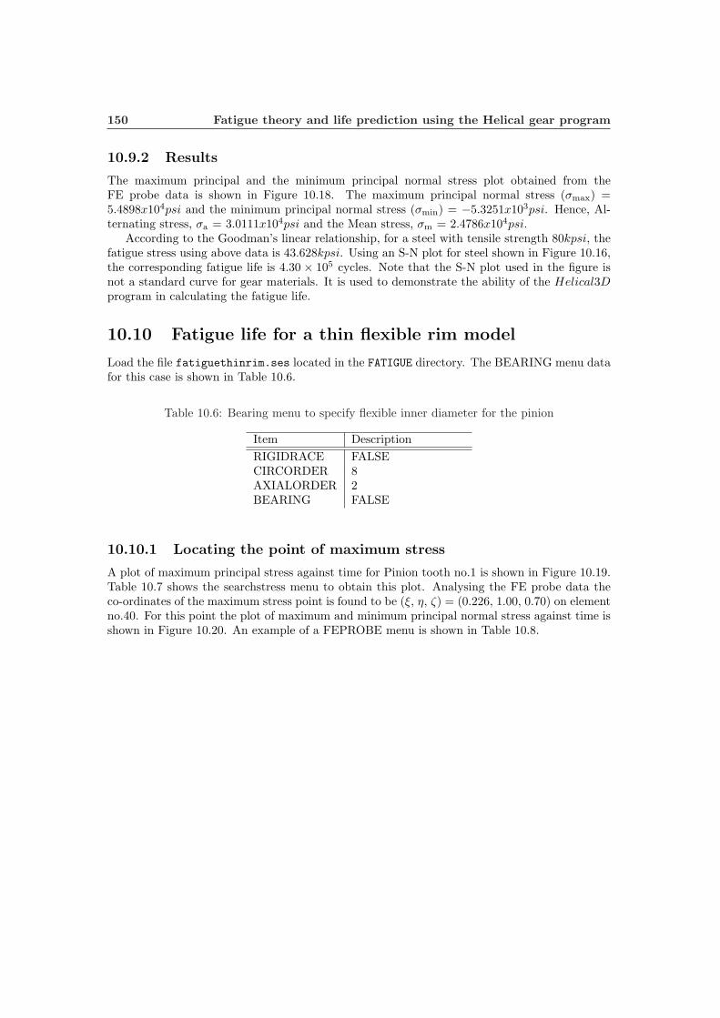
150 Fatigue theory and life prediction using the Helical gear program
10.9.2 Results
The maximum principal and the minimum principal normal stress plot obtained from theFE probe data is shown in Figure 10.18. The maximum principal normal stress (σmax) =5.4898x10⁴psi and the minimum principal normal stress (σmin) = −5.3251x10³psi. Hence, Al-ternating stress, σa = 3.0111x10⁴psi and the Mean stress, σm = 2.4786x10⁴psi.
According to the Goodman’s linear relationship, for a steel with tensile strength 80kpsi, thefatigue stress using above data is 43.628kpsi. Using an S-N plot for steel shown in Figure 10.16,the corresponding fatigue life is 4.30 × 10⁵ cycles. Note that the S-N plot used in the figure isnot a standard curve for gear materials. It is used to demonstrate the ability of the Helical3Dprogram in calculating the fatigue life.
10.10 Fatigue life for a thin flexible rim model
Load the file fatiguethinrim.ses located in the FATIGUE directory. The BEARING menu datafor this case is shown in Table 10.6.
Table 10.6: Bearing menu to specify flexible inner diameter for the pinion
Item DescriptionRIGIDRACE FALSECIRCORDER 8AXIALORDER 2BEARING FALSE
10.10.1 Locating the point of maximum stress
A plot of maximum principal stress against time for Pinion tooth no.1 is shown in Figure 10.19.Table 10.7 shows the searchstress menu to obtain this plot. Analysing the FE probe data theco-ordinates of the maximum stress point is found to be (ξ, η, ζ) = (0.226, 1.00, 0.70) on elementno.40. For this point the plot of maximum and minimum principal normal stress against time isshown in Figure 10.20. An example of a FEPROBE menu is shown in Table 10.8.
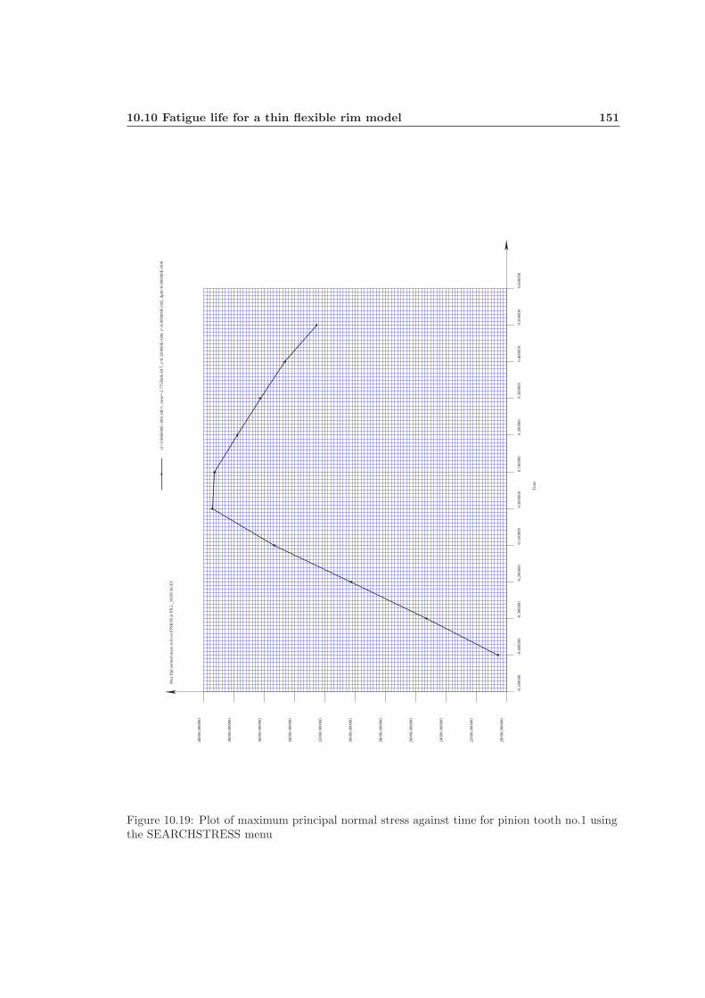
10.10 Fatigue life for a thin flexible rim model 151
-0.5
0000
0-0
.400
000
-0.3
0000
0-0
.200
000
-0.1
0000
0-0
.000
000
0.10
0000
0.20
0000
0.30
0000
0.40
0000
0.50
0000
0.60
0000
2000
0.00
0000
2200
0.00
0000
2400
0.00
0000
2600
0.00
0000
2800
0.00
0000
3000
0.00
0000
3200
0.00
0000
3400
0.00
0000
3600
0.00
0000
3800
0.00
0000
4000
0.00
0000
Tim
e
Max
Ppl
nor
mal
str
ess
(s1)
on
PIN
ION
at F
ILL
_SU
RFA
CE
1
s1=
3.94
6040
E+
004,
tth=
1, ti
me=
-2.7
7556
0E-0
17, s
=8.
3200
00E
+00
0, t=
-8.0
0000
0E-0
02, d
pth=
0.00
0000
E+
000
Figure 10.19: Plot of maximum principal normal stress against time for pinion tooth no.1 usingthe SEARCHSTRESS menu

152 Fatigue theory and life prediction using the Helical gear program
Table 10.7: Searchstress data
Item DescriptionCOMPONENT MAXPPLSTRESSXAXIS TIMEBEGINSTEP 1ENDSTEP 11BODY PINIONSURFACE FILLET1TOOTHBEGIN 1TOOTHEND 1SEPTEETH TRUESPROFBEGIN 6.00SPROFEND 12.00NUMSPROF 51TFACEBEGIN -0.5TFACEEND 0.5NUMTFACE 51DEPTHBEGIN 0.00DEPTHEND 0.00NUMDEPTH 1DISTMIN 0.05OUTPUTTOFILE TRUEFILENAME out.txtAPPEND TRUE
Table 10.8: FE probe data
Item DescriptionNPROBES 40PROBE 1BODY PINIONMESH TOOTHELEM 40XI 0.226ETA 1.00ZETA 0.70COMPONENT MAXPPLNORMALFILENAME PROBES.DAT
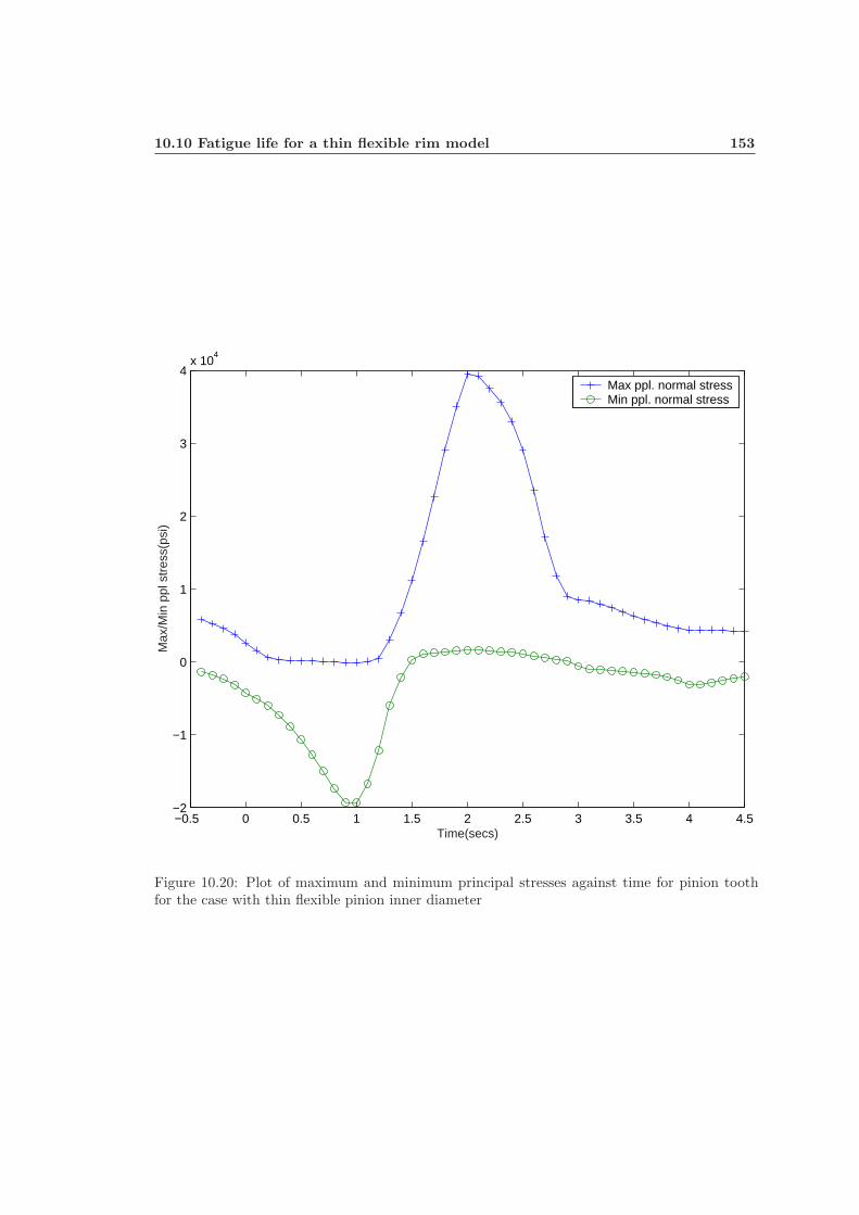
10.10 Fatigue life for a thin flexible rim model 153
−0.5 0 0.5 1 1.5 2 2.5 3 3.5 4 4.5−2
−1
0
1
2
3
4x 10
4
Time(secs)
Max
/Min
ppl
str
ess(
psi)
Max ppl. normal stressMin ppl. normal stress
Figure 10.20: Plot of maximum and minimum principal stresses against time for pinion toothfor the case with thin flexible pinion inner diameter

154 Fatigue theory and life prediction using the Helical gear program
10.10.2 Results
The maximum principal and the minimum principal normal stress plot obtained from theFE probe data is shown in Figure 10.20. The maximum principal normal stress (σmax) =3.9462x10⁴psi and the minimum principal normal stress (σmin) = −9.659x10³psi. Hence, Alter-nating stress, σa = 2.4560x10⁴psi and the Mean stress, σm = 1.49015x10⁴psi.
According to the Goodman’s linear relationship, for a steel with tensile strength 80kpsi, thefatigue stress using above data is 30.181kpsi. The fatigue life for this stress is almost infinite.
10.11 Cumulative damage
The S-N curves discussed in previous section are developed for constant stress amplitude op-eration. But, in virtually every engineering application where fatigue is an important failuremode, the alternating stress amplitude may be expected to vary or change in some way duringthe service life. Hence the usage of S-N curves in such cases is inapplicable. Therefore theoriesbased on cumulative damage are used while predicting fatigue failure.
The fatigue damage produced at any given cyclic stress amplitude will be related to the totalnumber of cycles of operation at that stress amplitude and also related to the total numberof cycles that would be required to produce failure of an undamaged specimen at that stressamplitude. It is further postulated that the damage incurred is permanent and operation atseveral different stress amplitudes in sequence will result in an accumulation of total damageequal to the sum of the damage increments accrued at each individual stress level. When thetotal accumulated damage reaches a critical value, fatigue failure occurs. Many different theoriesbased on this concept of cumulative damage have been proposed. We discuss here two theoriesvery commonly used for the purposes of assessing fatigue damage.
10.11.1 Linear damage theory
The linear damage theory is also referred as the Plamgren-Miner hypothesis or the linear damgerule. As discussed earlier the S-N curve(Figure 10.21) at a constant stress amplitude S1 willproduce complete damage, or failure, in N1 cycles. Operation at stress amplitude S1 for anumber of cycles n1 smaller than N1 will produce a smaller fraction of damage, D1. D1 isusually termed as the damage fraction. Operation over a spectrum of different stress levelsresults in a damage fraction Di for each of the different stress levels Si in the spectrum. Whenthis damage fractions sum to unity, failure is predicted, that is,
Failure is predicted to occur if:
D1 + D2 + ... + Di−1 + Di ≥ 1 (10.12)
The Palmgren-Miner hypothesis asserts that the damage fraction at any stress level Si islinearly proportional to the ratio of number of cycles of operation to the total number of cyclesthat would produce failure at that stress level, that is
Di =ni
Ni(10.13)
Thus we can also say that failure is predicted to occur if:
n1
N1+
n2
N2+ ... +
ni−1
Ni−1+
ni
Ni≥ 1 (10.14)
or failure is predicted to occur if:
i∑
j=1
nj
Nj≥ 1 (10.15)

10.11 Cumulative damage 155
Figure 10.21: S-N plot illustrating the linear damage theory

156 Fatigue theory and life prediction using the Helical gear program
Figure 10.22: S-N curve approximation proposed by Gatt
The Palmgren-Miner hypothesis is widely used because of its simplicity and the experimentalfact that the other much more complex cumulative damage theories do not always yield a signif-icant improvement in failure prediction reliability. The most significant drawback of the theorythough is that no influence of the order of application of various stress levels is recognized, anddamage is assumed to accumulate at the same rate at a given stress level without regard to pasthistory. Experimental data suggest that the order in which various stress levels are applied doeshave a significant influence and also that the damage rate at a given stress level is a function ofthe prior cyclic stress history.
10.11.2 Gatts Cumulative damage theory
Gatts postulated that the fatigue strength and the the fatigue limit change continuously withthe application of stress cycles, and that the change is proportional to a function of the stressamplitude.
The S-N curve3 according to the Gatt’s theory is given as:
kN =1
S − Se0
− 1S(1− C)
(10.16)
where,
3See Failure of materials in mechanical design by J.A. Collins.

10.12 Fatigue life based on duty cycle for a gear set 157
C, k = Material constant and proportionality constantSe0 = fatigue limit when N = 0Sq = Instantaneous value of strengthSe = Fatigue limit, a function of cyclic stress history, not a constant
= CSq
N = Number of cycles of stress appliedS = Amplitude of applied cyclic stress
Figure 10.22 shows the S-N curve based on the Gatt’s cumulative damage theory.Knowing the material properties and calculating the stress amplitude from the FE probe data
it is possible to calculate the fatigue life for a hypoid gear pair based on the Gatts cumulativedamage theory.
10.12 Fatigue life based on duty cycle for a gear set
We assume the gear set shown in example file fatigue.ses to be running at 90% of the totaltorque.
Load the file fatigueload1.ses located in the FATIGUE directory. We now run the gear setat about 110% of the total load(Torque=1222.22 lbf.in). For this load the maximum sress plotfrom the search stress menu is shown in Figure 10.23. The maximum stress point using the FEprobe data is found to be (0.546,1.00,0.91). For this point the maximum and minimum principalnormal stress plot is shown in Figure 10.25. The corresponding fatigue life hence obtained is6.0× 104cycles.
Load the file fatigueload2.ses located in the FATIGUE directory. We now run the gearset at 100% load(Torque = 1111.11lbf.in). For the point (0.546,1.00,0.91) on element no.40 themaximum and minimum principal normal stress plot is shown in Figure 10.24. The correspondingfatigue life hence obtained is 2.3× 10⁵cycles.
Load the file fatigueload3.ses located in the FATIGUE directory. We now run the gearset at Torque = 500lbf.in. For the point (0.546,1.00,0.91) on element no.40 the maximum andminimum principal normal stress plot is shown in Figure 10.26. The corresponding fatigue lifehence obtained is infinite.
Load the file fatigueload4.ses located in the FATIGUE directory. We now run the gear setat Torque = 1000lbf.in. For the point (0.546,1.00,0.91) on element no.40 the maximum andminimum principal normal stress plot is shown in Figure 10.27. The corresponding fatigue lifehence obtained is 5.2× 10⁵cycles.
The load and the corresponding fatigue life is summarised in Table 10.9.
Table 10.9: Fatigue life for a duty cycle
Torque(lbf-in) Fatiguelife(cycles)
Runningtime (%)
500 ∞ 70%1000 5.2e5 20%1111.11 2.3e5 9%1222.22 6.0e4 1%

158 Fatigue theory and life prediction using the Helical gear program
-0.6
0000
0-0
.400
000
-0.2
0000
0-0
.000
000
0.20
0000
0.40
0000
0.60
0000
0.80
0000
1.00
0000
3000
0.00
0000
4000
0.00
0000
5000
0.00
0000
6000
0.00
0000
7000
0.00
0000
Tim
e
Max
Ppl
nor
mal
str
ess
(s1)
on
PIN
ION
at F
ILL
_SU
RFA
CE
1
s1=
6.01
1540
E+
004,
tth=
1, ti
me=
1.00
0000
E-0
01, s
=7.
3600
00E
+00
0, t=
-2.0
0000
0E-0
02, d
pth=
0.00
0000
E+
000
Figure 10.23: Maximum principal normal stress plot against time for pinion tooth no.1 for aoutput torque of 1222.22 lbf.in

10.12 Fatigue life based on duty cycle for a gear set 159
−0.5 0 0.5 1 1.5 2 2.5 3 3.5 4 4.5−2
−1
0
1
2
3
4
5
6
7x 10
4
Time(secs)
Max
/Min
ppl
nor
mal
str
ess
(psi
)
Max ppl normal stressMin ppl normal stress
Figure 10.24: Maximum and minimum principal normal stress plot against time for pinion toothfor output torque of 1222.22 lbf.in

160 Fatigue theory and life prediction using the Helical gear program
−0.5 0 0.5 1 1.5 2 2.5 3 3.5 4 4.5−2
−1
0
1
2
3
4
5
6x 10
4
Time(secs)
Max
/Min
ppl
nor
mal
str
ess
(psi
)
Max ppl normal stressMin ppl normal stress
Figure 10.25: Maximum and minimum principal normal stress plot against time for pinion toothfor output torque of 1111.11 lbf.in

10.12 Fatigue life based on duty cycle for a gear set 161
−0.5 0 0.5 1 1.5 2 2.5 3 3.5 4 4.5−1
−0.5
0
0.5
1
1.5
2
2.5
3
3.5x 10
4
Time(s)
Max
/Min
ppl
nor
mal
str
ess(
psi)
Max ppl normal stressMin ppl normal stress
Figure 10.26: Maximum and minimum principal normal stress plot against time for pinion toothfor output torque of 500 lbf.in

162 Fatigue theory and life prediction using the Helical gear program
−0.5 0 0.5 1 1.5 2 2.5 3 3.5 4 4.5−2
−1
0
1
2
3
4
5
6x 10
4
Time(s)
Max
/Min
ppl
nor
mal
str
ess(
psi)
Max ppl normal stressMin ppl normal stress
Figure 10.27: Maximum and minimum principal normal stress plot against time for pinion toothfor output torque of 1000 lbf.in

10.13 Calculating life based on cumulative damage theory 163
10.13 Calculating life based on cumulative damage theory
From the Linear damage theory failure occurs when:
n1
N1+
n2
N2+ ... +
ni−1
Ni−1+
ni
Ni= 1 (10.17)
Substituting the values from Table 10.9 in the above we get:
0.7n
∞ +0.2n
5.2× 10⁵+
0.09n
2.3× 10⁵+
0.01n
6.0× 104= 1 (10.18)
Thus, the life cycle for the gear set is 1.06091× 10⁶cycles.
10.14 Conclusions
Helical3D program can be employed to calculate the fatigue life for gear bodies. Although forthe example cases we gave considered a helical gear pair the same procedure can be applied tospur gear pair. As can be seen from the Table 10.9 as the load increases the fatigue life is foundto decrease as expected. We feel calyx gives a reasonable approach towards calculation of fatiguelife although we cannot verify the results obtained from Calyx with experimental or analyticalcalculations due to lack of information at this time.

164 Fatigue theory and life prediction using the Helical gear program
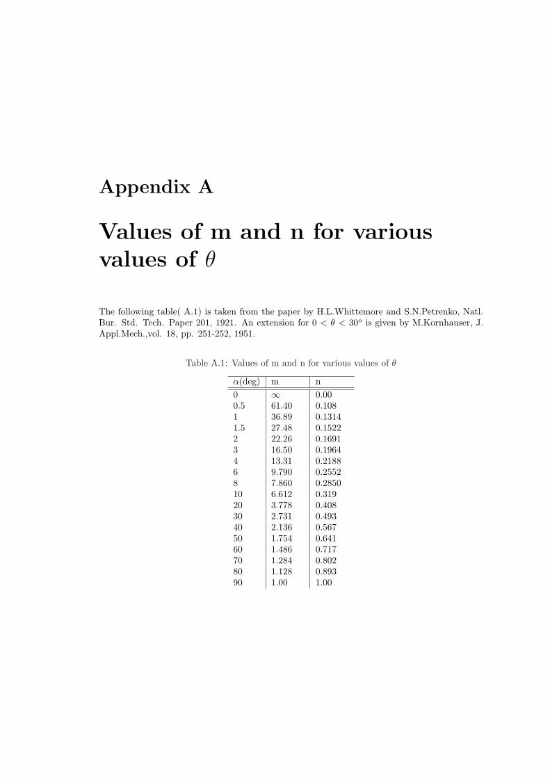
Appendix A
Values of m and n for variousvalues of θ
The following table( A.1) is taken from the paper by H.L.Whittemore and S.N.Petrenko, Natl.Bur. Std. Tech. Paper 201, 1921. An extension for 0 < θ < 30o is given by M.Kornhauser, J.Appl.Mech.,vol. 18, pp. 251-252, 1951.
Table A.1: Values of m and n for various values of θ
α(deg) m n0 ∞ 0.000.5 61.40 0.1081 36.89 0.13141.5 27.48 0.15222 22.26 0.16913 16.50 0.19644 13.31 0.21886 9.790 0.25528 7.860 0.285010 6.612 0.31920 3.778 0.40830 2.731 0.49340 2.136 0.56750 1.754 0.64160 1.486 0.71770 1.284 0.80280 1.128 0.89390 1.00 1.00

166 Values of m and n for various values of θ
Bibliography
[1] Planetary Gear Train Ring Gear and Support Structure Investigation, Mark Valco, Ph.D.Dissertation, Cleveland State University, 1992.
[2] Gear Tooth Stress Measurements of Two Helicopter Planetary Stages, Krantz, T. L., NASATechnical Memorandum 105651, AVSCOM Technical Report 91-C-038, 1992.
[3] A combined surface integral and finite element solution for a three-dimensional contactproblem, S. Vijayakar, International Journal for Numerical Methods in Engineering, vol.31,pp. 525-545, 1991.
[4] Nonlinear and dynamic programming, G. Hadley, Addison Wesley Publishing company,1964.
[5] Linear programming, George Hadley, Addison Wesley, 1962.
[6] Linear and Combinatorial Programming, Katta G. Murty, John Wiley, 1976 ISBN: 0-471-57370-1.
[7] Linearization of multibody frictional contact problems, S. Vijayakar, H. Busby and D.Houser, Computers and Structures, vol. 29, no. 4, pp. 569-576, 1987.
[8] Natural Frequency Spectra and Vibration Modes of Planetary Gears, Jian Lin and RobertParker, 1998 ASME Design Engineering Technical Conference, September 1998, AtlantaGeorgia.
[9] Gear Dynamics Experiments, Part I: Characterization of Forced Response, Blankenshipand Kahraman, ASME 7th International Power Transmissions and Gearing Conference,San Diego, October 1996.
[10] Gear Dynamics Experiments, Part II: Effect of Involute Contact Ratio, Blankenship andKahraman, ASME 7th International Power Transmissions and Gearing Conference, SanDiego, October 1996.
[11] Gear Dynamics Experiments, Part III: Effect of Involute Tip Relief, Blankenship and Kahra-man, ASME 7th International Power Transmissions and Gearing Conference, San Diego,October 1996.
[12] The use of boundary elements for the determination of the geometry factor, Vijayakar andHouser, 1986 AGMA Fall Technical Meeting, Paper no. 86-FTM-10.
[13] Finite element analysis of quasi-prismatic structures, S. Vijayakar, H. Busby and D. Houser,International Journal for Numerical Methods in Engineering, vol. 24, pp. 1461-1477, 1987.
[14] Edge effects in gear tooth contact, S. Vijayakar, ASME 7th International Power Transmis-sions and Gearing Conference, San Diego, October 1996.

168 BIBLIOGRAPHY
[15] Vibration Measurements on Planetary Gears of Aircraft Turbine Engines, M. Botman,AIAA Journal, vol. 17, no. 5, 1980.
[16] Dynamic Tooth Loads in Epicyclic Gears, F. Cunliffe, J. D. Smith, and D.B. Welbourn, J.Eng. Ind. Trans. ASME, May 1974.
[17] Effect of Internal Gear Flexibility on the Quassi-Static Behavior of a Planetary Gear Set,A. Kahraman, S. Vijayakar, Transactions of the ASME, September 2001.
[18] Study on bending fatigue strength of Helical gears, Oda, Koide, Bull.JSME, Vol 26, 1983.
[19] Bending strength estimation of thin-rimmed spur gears, Oda, Miyachika, Transactions ofthe ASME, October 1996.
[20] Contact Mechanics, Johnson, K. L., Cambridge University Press, 1985
[21] Theoryof Elasticity, Timoshenko and Goodier, Mcgraw-Hill publication, Third Edition, 1970
[22] Analysis of spur and helical gears using a combination of finite element and surface integraltechniques, Avinashchandra Singh, The Ohio State University, M.S. Thesis, 1992