TERRESTRIAL HYDROMETEOROLOGY - Universidad ZamoranoTERRESTRIAL HYDROMETEOROLOGY W. JAMES...
473
TERRESTRIAL HYDROMETEOROLOGY
Transcript of TERRESTRIAL HYDROMETEOROLOGY - Universidad ZamoranoTERRESTRIAL HYDROMETEOROLOGY W. JAMES...
TERRESTRIAL HYDROMETEOROLOGY
Shuttleworth_ffirs.indd iShuttleworth_ffirs.indd i 11/3/2011 10:06:59 AM11/3/2011 10:06:59 AM

COMPANION WEBSITE
This book has a companion website:
www.wiley.com/go/shuttleworth/hydrometeorology
with Figures and Tables from the book for downloading
Shuttleworth_ffirs.indd iiShuttleworth_ffirs.indd ii 11/3/2011 10:06:59 AM11/3/2011 10:06:59 AM

TERRESTRIAL HYDROMETEOROLOGY
W. JAMES SHUTTLEWORTH
A John Wiley & Sons, Ltd., Publication
Shuttleworth_ffirs.indd iiiShuttleworth_ffirs.indd iii 11/3/2011 10:06:59 AM11/3/2011 10:06:59 AM
This edition first published 2012
© 2012 by John Wiley & Sons, Ltd
Wiley-Blackwell is an imprint of John Wiley & Sons, formed by the merger of Wiley’s global
Scientific, Technical and Medical business with Blackwell Publishing.
Registered office
John Wiley & Sons, Ltd, The Atrium, Southern Gate, Chichester, West Sussex, PO19 8SQ, UK
Editorial offices
9600 Garsington Road, Oxford, OX4 2DQ, UK
The Atrium, Southern Gate, Chichester, West Sussex, PO19 8SQ, UK
111 River Street, Hoboken, NJ 07030-5774, USA
For details of our global editorial offices, for customer services and for information about how
to apply for permission to reuse the copyright material in this book please see our website at
www.wiley.com/wiley-blackwell.
The right of the author to be identified as the author of this work has been asserted in
accordance with the UK Copyright, Designs and Patents Act 1988.
All rights reserved. No part of this publication may be reproduced, stored in a retrieval system,
or transmitted, in any form or by any means, electronic, mechanical, photocopying, recording
or otherwise, except as permitted by the UK Copyright, Designs and Patents Act 1988, without
the prior permission of the publisher.
Designations used by companies to distinguish their products are often claimed as trademarks.
All brand names and product names used in this book are trade names, service marks,
trademarks or registered trademarks of their respective owners. The publisher is not associated
with any product or vendor mentioned in this book. This publication is designed to provide
accurate and authoritative information in regard to the subject matter covered. It is sold on the
understanding that the publisher is not engaged in rendering professional services. If
professional advice or other expert assistance is required, the services of a competent
professional should be sought.
Library of Congress Cataloging-in-Publication Data
Shuttleworth, W. James.
Terrestrial hydrometeorology / W. James Shuttleworth.
p. cm.
ISBN 978-0-470-65938-0 (hardback) – ISBN 978-0-470-65937-3 (paper) 1. Hydrometeorology–
Textbooks. I. Title.
GB2803.2.S58 2012
551.57–dc23
2011041765
A catalogue record for this book is available from the British Library.
Set in 10/12.5pt Minion Pro by SPi Publisher Services, Pondicherry, India
1 2012
Shuttleworth_ffirs.indd ivShuttleworth_ffirs.indd iv 11/3/2011 10:07:00 AM11/3/2011 10:07:00 AM

This book is dedicated with love and gratitude to Hazel, Craig, Matthew, Nicholas, Jonathan and Amy for all the
good and worthwhile things they have brought into my life.
Shuttleworth_ffirs.indd vShuttleworth_ffirs.indd v 11/3/2011 10:07:00 AM11/3/2011 10:07:00 AM
Contents
Foreword xvi
Preface xviii
Acknowledgements xix
1 Terrestrial Hydrometeorology and the Global Water Cycle 1
Introduction 1
Water in the Earth system 2
Components of the global hydroclimate system 4
Atmosphere 5
Hydrosphere 8
Cryosphere 9
Lithosphere 9
Biosphere 10
Anthroposphere 10
Important points in this chapter 12
2 Water Vapor in the Atmosphere 14
Introduction 14
Latent heat 14
Atmospheric water vapor content 15
Ideal Gas Law 16
Virtual temperature 17
Saturated vapor pressure 18
Measures of saturation 20
Measuring the vapor pressure of air 21
Important points in this chapter 23
3 Vertical Gradients in the Atmosphere 25
Introduction 25
Hydrostatic pressure law 26
Adiabatic lapse rates 27
Dry adiabatic lapse rate 27
Moist adiabatic lapse rate 28
Environmental lapse rate 28
Vertical pressure and temperature gradients 29
Potential temperature 30
Virtual potential temperature 31
Shuttleworth_ftoc.indd viiShuttleworth_ftoc.indd vii 11/3/2011 10:06:53 AM11/3/2011 10:06:53 AM
viii Contents
Atmospheric stability 32
Static stability parameter 32
Important points in this chapter 34
4 Surface Energy Fluxes 36
Introduction 36
Latent and sensible heat fluxes 37
Energy balance of an ideal surface 38
Net radiation, Rn 38
Latent heat flux, lE 39
Sensible heat flux, H 39
Soil heat flux, G 39
Physical energy storage, St 40
Biochemical energy storage, P 40
Advected energy, Ad 41
Flux sign convention 41
Evaporative fraction and Bowen ratio 45
Energy budget of open water 46
Important points in this chapter 46
5 Terrestrial Radiation 48
Introduction 48
Blackbody radiation laws 49
Radiation exchange for ‘gray’ surfaces 51
Integrated radiation parameters for natural surfaces 52
Maximum solar radiation at the top of atmosphere 54
Maximum solar radiation at the ground 56
Atmospheric attenuation of solar radiation 58
Actual solar radiation at the ground 59
Longwave radiation 59
Net radiation at the surface 62
Height dependence of net radiation 63
Important points in this chapter 64
6 Soil Temperature and Heat Flux 66
Introduction 66
Soil surface temperature 66
Subsurface soil temperatures 67
Thermal properties of soil 68
Density of soil, rs 69
Specific heat of soil, cs 70
Heat capacity per unit volume, Cs 70
Thermal conductivity, ks 70
Thermal diffusivity, as 71
Formal description of soil heat flow 71
Thermal waves in homogeneous soil 72
Important points in this chapter 75
Shuttleworth_ftoc.indd viiiShuttleworth_ftoc.indd viii 11/3/2011 10:06:54 AM11/3/2011 10:06:54 AM
Contents ix
7 Measuring Surface Heat Fluxes 77
Introduction 77
Measuring solar radiation 77
Daily estimates of cloud cover 77
Thermoelectric pyranometers 78
Photoelectric pyranometers 79
Measuring net radiation 80
Measuring soil heat flux 81
Measuring latent and sensible heat 82
Micrometeorological measurement of surface energy fluxes 83
Bowen ratio/energy budget method 83
Eddy correlation method 85
Evaporation measurement from integrated water loss 87
Evaporation pans 88
Watersheds and lakes 89
Lysimeters 90
Soil moisture depletion 91
Comparison of evaporation measuring methods 91
Important points in this chapter 94
8 General Circulation Models 96
Introduction 96
What are General Circulation Models? 96
How are General Circulation Models used? 98
How do General Circulation Models work? 100
Sequence of operations 100
Solving the dynamics 102
Calculating the physics 103
Intergovernmental Panel on Climate Change (IPCC) 104
Important points in this chapter 105
9 Global Scale Influences on Hydrometeorology 107
Introduction 107
Global scale influences on atmospheric circulation 107
Planetary interrelationship 109
Latitudinal differences in solar energy input 109
Seasonal perturbations 109
Daily perturbations 109
Persistent perturbations 109
Contrast in ocean to continent surface exchanges 109
Continental topography 109
Temporary perturbations 110
Perturbations in oceanic circulation 110
Perturbations in atmospheric content 110
Perturbations in continental land cover 110
Latitudinal imbalance in radiant energy 110
Shuttleworth_ftoc.indd ixShuttleworth_ftoc.indd ix 11/3/2011 10:06:54 AM11/3/2011 10:06:54 AM
x Contents
Lower atmosphere circulation 111
Latitudinal bands of pressure and wind 111
Hadley circulation 112
Mean low-level circulation 113
Mean upper level circulation 115
Ocean circulation 116
Oceanic influences on continental hydroclimate 118
Monsoon flow 118
Tropical cyclones 119
El Niño Southern Oscillation 120
Pacific Decadal Oscillation 122
North Atlantic Oscillation 123
Water vapor in the atmosphere 123
Important points in this chapter 126
10 Formation of Clouds 128
Introduction 128
Cloud generating mechanisms 129
Cloud condensation nuclei 131
Saturated vapor pressure of curved surfaces 132
Cloud droplet size, concentration and terminal velocity 133
Ice in clouds 134
Cloud formation processes 135
Thermal convection 135
Foehn effect 136
Extratropical fronts and cyclones 138
Cloud genera 140
Important points in this chapter 141
11 Formation of Precipitation 143
Introduction 143
Precipitation formation in warm clouds 144
Precipitation formation in other clouds 146
Which clouds produce rain? 148
Precipitation form 149
Raindrop size distribution 150
Rainfall rates and kinetic energy 151
Forms of frozen precipitation 151
Other forms of precipitation 152
Important points in this chapter 153
12 Precipitation Measurement and Observation 155
Introduction 155
Precipitation measurement using gauges 156
Instrumental errors 157
Site and location errors 157
Shuttleworth_ftoc.indd xShuttleworth_ftoc.indd x 11/3/2011 10:06:54 AM11/3/2011 10:06:54 AM
Contents xi
Gauge designs 160
Areal representativeness of gauge measurements 162
Snowfall measurement 165
Precipitation measurement using ground-based radar 168
Precipitation measurement using satellite systems 171
Cloud mapping and characterization 171
Passive measurement of cloud properties 172
Spaceborne radar 173
Important points in this chapter 174
13 Precipitation Analysis in Time 176
Introduction 176
Precipitation climatology 177
Annual variations 177
Intra-annual variations 177
Daily variations 180
Trends in precipitation 181
Running means 182
Cumulative deviations 183
Mass curve 184
Oscillations in precipitation 186
System signatures 187
Intensity-duration relationships 189
Statistics of extremes 190
Conditional probabilities 195
Important points in this chapter 196
14 Precipitation Analysis in Space 198
Introduction 198
Mapping precipitation 199
Areal mean precipitation 200
Isohyetal method 200
Triangle method 202
Theissen method 202
Spatial organization of precipitation 203
Design storms and areal reduction factors 205
Probable maximum precipitation 207
Spatial correlation of precipitation 209
Important points in this chapter 211
15 Mathematical and Conceptual Tools of Turbulence 213
Introduction 213
Signature and spectrum of atmospheric turbulence 213
Mean and fluctuating components 216
Rules of averaging for decomposed variables 217
Variance and standard deviation 219
Shuttleworth_ftoc.indd xiShuttleworth_ftoc.indd xi 11/3/2011 10:06:54 AM11/3/2011 10:06:54 AM
xii Contents
Measures of the strength of turbulence 220
Mean and turbulent kinetic energy 220
Linear correlation coefficient 221
Kinematic flux 223
Advective and turbulent fluxes 225
Important points in this chapter 229
16 Equations of Atmospheric Flow in the ABL 231
Introduction 231
Time rate of change in a fluid 232
Conservation of momentum in the atmosphere 234
Pressure forces 235
Viscous flow in fluids 236
Axis-specific forces 239
Combined momentum forces 242
Conservation of mass of air 243
Conservation of atmospheric moisture 244
Conservation of energy 245
Conservation of a scalar quantity 246
Summary of equations of atmospheric flow 247
Important points in this chapter 247
17 Equations of Turbulent Flow in the ABL 248
Introduction 248
Fluctuations in the ideal gas law 248
The Boussinesq approximation 249
Neglecting subsidence 250
Geostrophic wind 251
Divergence equation for turbulent fluctuations 252
Conservation of momentum in the turbulent ABL 252
Conservation of moisture, heat, and scalars
in the turbulent ABL 254
Neglecting molecular diffusion 255
Important points in this chapter 258
18 Observed ABL Profiles: Higher Order Moments 259
Introduction 259
Nature and evolution of the ABL 259
Daytime ABL profiles 261
Nighttime ABL profiles 263
Higher order moments 265
Prognostic equations for turbulent departures 265
Prognostic equations for turbulent kinetic energy 269
Prognostic equations for variance of moisture and heat 271
Important points in this chapter 276
Shuttleworth_ftoc.indd xiiShuttleworth_ftoc.indd xii 11/3/2011 10:06:54 AM11/3/2011 10:06:54 AM
Contents xiii
19 Turbulent Closure, K Theory, and Mixing Length 277
Introduction 277
Richardson number 277
Turbulent closure 279
Low order closure schemes 280
Local, first order closure 281
Mixing length theory 283
Important points in this chapter 288
20 Surface Layer Scaling and Aerodynamic Resistance 289
Introduction 289
Dimensionless gradients 290
Obukhov length 292
Flux-gradient relationships 293
Returning fluxes to natural units 294
Resistance analogues and aerodynamic resistance 296
Important points in this chapter 299
21 Canopy Processes and Canopy Resistances 300
Introduction 300
Boundary layer exchange processes 301
Shelter factors 306
Stomatal resistance 308
Energy budget of a dry leaf 310
Energy budget of a dry canopy 311
Important points in this chapter 314
22 Whole Canopy Interactions 316
Introduction 316
Whole-canopy aerodynamics and canopy structure 317
Excess resistance 319
Roughness sublayer 321
Wet canopies 323
Equilibrium evaporation 325
Evaporation into an unsaturated atmosphere 327
Important points in this chapter 332
23 Daily Estimates of Evaporation 334
Introduction 334
Daily average values of weather variables 335
Temperature, humidity, and wind speed 335
Net radiation 337
Open water evaporation 339
Reference crop evapotranspiration 341
Penman-Monteith equation estimation of ERC
342
Shuttleworth_ftoc.indd xiiiShuttleworth_ftoc.indd xiii 11/3/2011 10:06:54 AM11/3/2011 10:06:54 AM
xiv Contents
Radiation-based estimation of ERC
344
Temperature-based estimation of ERC
345
Evaporation pan-based estimation of ERC
346
Evaporation from unstressed vegetation: the Matt-Shuttleworth
approach 348
Evaporation from water stressed vegetation 353
Important points in this chapter 355
24 Soil Vegetation Atmosphere Transfer Schemes 359
Introduction 359
Basis and origin of land-surface sub-models 359
Developing realism in SVATS 362
Plot-scale, one-dimensional ‘micrometeorological’ models 364
Improving representation of hydrological processes 367
Improving representation of carbon dioxide exchange 368
Ongoing developments in land surface sub-models 370
Important points in this chapter 373
25 Sensitivity to Land Surface Exchanges 380
Introduction 380
Influence of land surfaces on weather and climate 381
A. The influence of existing land-atmosphere interactions 383
1. Effect of topography on convection and precipitation 383
2. Contribution by land surfaces to atmospheric
water availability 385
B. The influence of transient changes in land surfaces 385
1. Effect of transient changes in soil moisture 385
2. Effect of transient changes in vegetation cover 388
3. Effect of transient changes in frozen precipitation cover 389
4. Combined effect of transient changes 391
C. The influence of imposed persistent changes in land cover 392
1. Effect of imposed land cover change on near
surface observations 392
2. Effect of imposed land-cover change on
regional-scale climate 393
3. Effect of imposed heterogeneity in land cover 395
Important points in this chapter 398
26 Example Questions and Answers 404
Introduction 404
Example questions 404
Question 1 404
Question 2 405
Question 3 407
Question 4 408
Question 5 410
Shuttleworth_ftoc.indd xivShuttleworth_ftoc.indd xiv 11/3/2011 10:06:54 AM11/3/2011 10:06:54 AM

Contents xv
Question 6 411
Question 7 412
Question 8 414
Question 9 416
Question 10 418
Example Answers 418
Answer 1 418
Answer 2 420
Answer 3 420
Answer 4 425
Answer 5 426
Answer 6 427
Answer 7 429
Answer 8 432
Answer 9 434
Answer 10 437
Index 441
COMPANION WEBSITE
This book has a companion website:
www.wiley.com/go/shuttleworth/hydrometeorology
with Figures and Tables from the book for downloading
Shuttleworth_ftoc.indd xvShuttleworth_ftoc.indd xv 11/3/2011 10:06:54 AM11/3/2011 10:06:54 AM
Foreword
As a doctoral student of hydrology in the 1970s my only exposure to the
meteorological aspects of the hydrologic cycle was a few introductory chapters in
hydrology textbooks. These were limited in scope because class emphasis was on
the surface and subsurface water flow. Coverage of precipitation and evaporation
were also limited to single brief chapters, and there was no exposure to the
interface between meteorology and hydrology. Since then there has been a
complete transformation. The discipline of hydrometeorology has evolved
rapidly due to advances in observational technologies and large scale modeling,
both stimulated by the scientific need to address emerging issues such as climate
change and the requirement to provide water resources to a growing global
population. International programs such as the Global Energy and Water Cycle
EXperiment (GEWEX) initiated by the World Climate Research Programme and
the Biospheric Aspects of the Hydrologic Cycle (BAHC) initiated by the
International Geosphere Biosphere Program heightened interest in the coupling
between atmospheric and the terrestrial systems. But the many scientists and
students involved in this new interdisciplinary research had to gain their
knowledge of the two fields in piecemeal fashion. A textbook was obviously
needed to bridge the two disciplines.
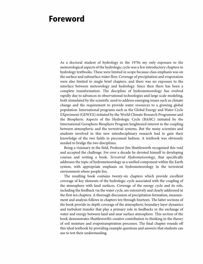
Being a visionary in the field, Professor Jim Shuttleworth recognized this void
and accepted the challenge. For over a decade he devoted himself to developing
courses and writing a book, Terrestrial Hydrometeorology, that specifically
addresses the topic of hydrometeorology as a unified component within the Earth
system, with appropriate emphasis on hydrometeorology in the terrestrial
environment where people live.
The resulting book contains twenty-six chapters which provide excellent
coverage of key elements of the hydrologic cycle associated with the coupling of
the atmosphere with land surfaces. Coverage of the energy cycle and its role,
including the feedback via the water cycle, are extensively and clearly addressed in
the first ten chapters. A thorough discussion of precipitation formation, measure-
ment and analysis follows in chapters ten through fourteen. The latter sections of
the book provide in-depth coverage of the atmospheric boundary layer dynamics
and turbulent transfer that play a primary role in feedbacks in the exchange of
water and energy between land and near surface atmosphere. This section of the
book demonstrates Shuttleworth’s creative contribution to thinking in the theory
of soil moisture and evapotranspiration processes. The final chapter rounds off
this ideal textbook by providing example questions and answers that students can
use to test their understanding.
Shuttleworth_fbetw.indd xviShuttleworth_fbetw.indd xvi 11/3/2011 10:06:48 AM11/3/2011 10:06:48 AM

Foreword xvii
It is exciting to finally have a single textbook on terrestrial hydrometeorology
that is balanced, timely and elegant, and that will be appropriate for use in graduate
courses for many years to come. Terrestrial Hydrometeorology will provide
opportunity for atmospheric science and hydrology programs to develop courses
that satisfy their cross-disciplinary educational requirements and, in this way, play
an important role in the education of the new generation of interdisciplinary
scientists who investigate the complex role of the hydrologic cycle in the climate
system. For many academics such a book would be the capstone publication of
their career but, knowing Jim Shuttleworth as I do, I am certain that we can expect
more such creative contributions in the future!
Soroosh Sorooshian
Director of the Center for Hydrometeorology and Remote Sensing
Distinguished Professor of Civil and Environmental Engineering
and Earth System Science at the University of California – Irvine
Shuttleworth_fbetw.indd xviiShuttleworth_fbetw.indd xvii 11/3/2011 10:06:48 AM11/3/2011 10:06:48 AM
Preface
Water is the medium through which the atmosphere has most influence on human
wellbeing and terrestrial surfaces have significant influence on the atmosphere.
Hitherto atmospheric and hydrologic science and practice have largely developed
separately. To hydrologists, meteorological variables were monitored and used as
independent forcing in models of hydrological responses. But hydrologists now
understand that near-surface meteorology is itself in part determined by how
surface water moves and how much water the land surface returns to the
atmosphere as evaporation. Consequently, graduate-level hydrological training
must now include relevant aspects of meteorological science. To meteorologists,
atmospheric exchanges with the land surface were regarded as boundary conditions
that could be calculated simply, with corrections to weather forecast models then
made by assimilating meteorological observations. But because about half the
energy that drives the atmosphere enters from below, meteorological forecasts
beyond a few days, and climate predictions in particular, require models that
include adequately realistic sub-models of surface hydrology and associated
energy exchanges. Consequently, graduate-level meteorological training must
now include relevant aspects of hydrological science. In fact the relationship
between hydrologists and meteorologists and their need to speak a common
scientific language is such that it is now recognized that a new science discipline
that overlies the land-atmosphere interface is needed, and courses that teach this
new discipline of Hydrometeorology are now being created at universities.
Hitherto there has been no single graduate-level text with sufficient breadth
across the hydrological and meteorological sciences that provides understanding
with adequate depth in both disciplines for use in hydrology departments to teach
relevant aspects of meteorology, in meteorological departments to teach relevant
aspects of surface hydrology, and to serve as an introductory text to teach the
emerging discipline of hydrometeorology. The primary intended readership of
this book is, therefore, graduate students studying surface water hydrology,
meteorology, and hydrometeorology. However this book could be used in relevant
advanced undergraduate courses and it will likely also find broader readership
among scientists seeking to broaden their education.
Shuttleworth_fpref.indd xviiiShuttleworth_fpref.indd xviii 11/3/2011 10:06:41 AM11/3/2011 10:06:41 AM

Acknowledgments
This book was written in response to a need for an appropriate text for use in
teaching a core course in the University of Arizona Hydrometeorology Program.
That course was based on an existing course taught by the author in the
Hydrology and Water Resources Program that had evolved over the years in
response to students’ needs and students’ input. The resulting syllabus ultimately
determined the content of this book. I would, therefore, like to thank all the
many students who contributed to that evolution and who have in this way
participated in the definition of Terrestrial Hydrometeorology, both the subject
and the text book. The manuscript was largely written while the author was on
sabbatical leave as a Fellow of the Joint Centre for Hydro-Meteorological
Research (JCHMR) which is located in the Centre for Ecology and Hydrology
(CEH), Wallingford, UK. I am grateful for the support and the friendship I
received from everyone at the CEH, and in particular I would like to thank
Richard Harding, Eleanor Blyth, Bob Moore, Martin Best, and Alan Jenkins for
facilitating my pleasant and rewarding time at JCHMR. The NSF Science and
Technology Center for Sustainability of semi-Arid and Riparian Areas (SAHRA)
provided partial financial support during that period and also subsequently
supported the refinement of this text through the patience and precision of
Annisa Tangreen who provided copy editing support for the manuscript. I am
pleased to acknowledge the support of SAHRA, and Annisa in particular.
I would also like to thank my good friend and ex-colleague, John Gash, who
carefully checked for typographic errors in equations and made a final review of
the manuscript, and I am also happy to acknowledge Xu Liang of University of
Pittsburg for advice and her input to the review of SVATS given in Chapter 24.
Finally, I would like to give my wholehearted thanks to my wife, Hazel, for her
immense patience through the many exacting hours it took to prepare this text,
for her cheerfulness when the writing was difficult, and the gin-and-tonics we
shared when it was just too difficult!
Shuttleworth_flast.indd xixShuttleworth_flast.indd xix 11/3/2011 8:37:13 PM11/3/2011 8:37:13 PM
Landprecipitation
113
Land
Riverslakes178
Soil moisture122Ocean
1,335,040
Surface flow
Ground water flow
Oceanevaporation 413
Oceanprecipitation
373
Ocean to landwater vapor transport
40
Atmosphere12.7
Groundwater15,300
Permafrost22
Vegetation
Percolation
40
Evaporation, transpiration 73
Ocean
Ice26,350
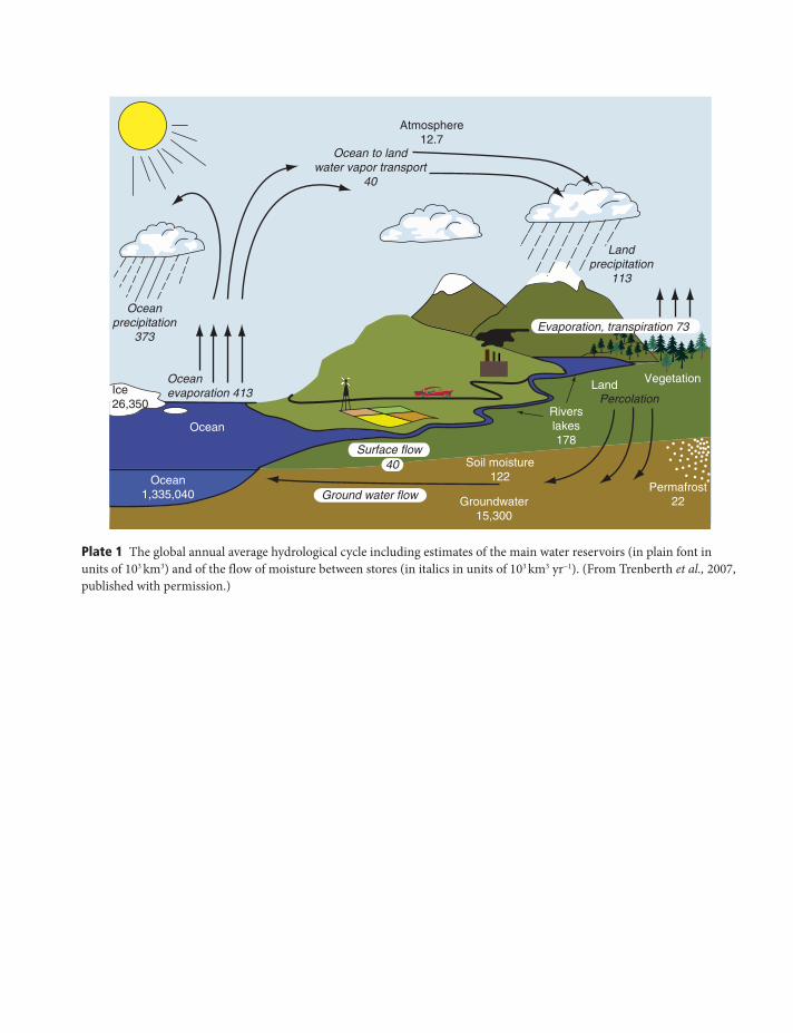
Plate 1 The global annual average hydrological cycle including estimates of the main water reservoirs (in plain font in
units of 103 km3) and of the flow of moisture between stores (in italics in units of 103 km3 yr−1). (From Trenberth et al., 2007,
published with permission.)
Shuttleworth_bins.indd 1Shuttleworth_bins.indd 1 11/3/2011 5:39:26 PM11/3/2011 5:39:26 PM
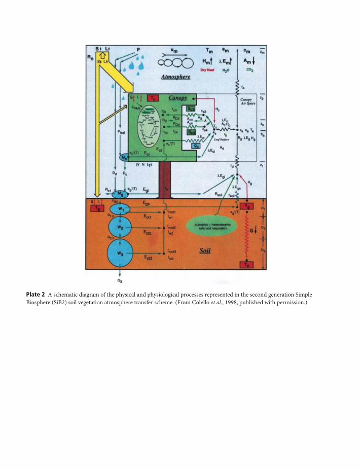
Plate 2 A schematic diagram of the physical and physiological processes represented in the second generation Simple
Biosphere (SiB2) soil vegetation atmosphere transfer scheme. (From Colello et al., 1998, published with permission.)
Shuttleworth_bins.indd 2Shuttleworth_bins.indd 2 11/3/2011 5:39:28 PM11/3/2011 5:39:28 PM
lE
lE
lEH
H
H Sr
Lu
Lu
LuSr
Sr lEH
Lu
SrlE
H
Lu
Sr
P S Ld
Runoff
Runoff
RunoffRunoff
Bare soil
Snow pack
Deep drainageDeep drainage
Deep drainage
Deep drainage
Plate 3 Schematic diagram of second generation one-dimensional SVATs in which a plot-scale micrometeorological model
with an explicit vegetation canopy was applied at grid scale.
Mixedvegetation
grid squares
S
lE
lElE
lE
H
HH
H
Sr
SrSr
Sr
Snow pack
Water table
Bare soil
P
m
1-m
Fractional precipitation on each grid
Topography
Lu
Lu
Lu
Lu
Ld
Plate 4 Schematic diagram of SVATS with improved representation of hydrologic processes.
Shuttleworth_bins.indd 3Shuttleworth_bins.indd 3 11/3/2011 5:39:30 PM11/3/2011 5:39:30 PM
Vegetationdynamics Vegetation
growth cycle
CO2
N2
lE
lE
lE
H
H
H Sr
Lu
Lu
LuSr
Sr lEH
Lu
SrlE
H
Lu
Sr
PS Ld
Runoff
Snow pack Runoff
RunoffRunoff
Bare soil
Deep drainageDeep drainage
Deep drainage
Deep drainage
Plate 5 Schematic diagram of SVATS with improved representation of vegetation related processes, including CO2
exchange and ecosystem evolution.
Mixed vegetationwith vegetation
dynamics
SLd
(CO2, N2,...)
Dataassimilation
m
1-m
Fractional precipitation on each grid
(CO2, N2,...)
LuLu
SrSr
HH
lElE
Snowpack
Routing
Routing
Plate 6 Schematic diagram of potential future developments in SVATS.
Shuttleworth_bins.indd 4Shuttleworth_bins.indd 4 11/3/2011 5:39:34 PM11/3/2011 5:39:34 PM
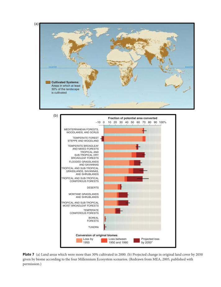
Cultivated Systems:Areas in which at least30% of the landscapeis cultivated
(a)
MEDITERRANEAN FORESTS,WOODLANDS, AND SCRUS
TEMPERATE FORESTSTEPPE AND WOODLAND
TEMPERATE BROADLEAFAND MIXED FORESTS
TROPICAL ANDSUB-TROPICAL DRY
BROADLEAF FORESTS
FLOODED GRASSLANDSAND SAVANNAS
TROPICAL AND SUB-TROPICALGRASSLANDS, SAVANNAS,
AND SHRUBLANDS
TROPICAL AND SUB-TROPICALCONIFEROUS FORESTS
DESERTS
MONTANE GRASSLANDSAND SHRUBLANDS
TROPICAL AND SUB-TROPICALMOIST BROADLEAF FORESTS
TEMPERATECONIFEROUS FORESTS
BOREALFORESTS
TUNDRA
Conversion of original biomesLoss by1950
Fraction of potential area converted−10 0 10 20 30 40 50 60 70 80 90 100%
Loss between1950 and 1990
Projected lossby 2050*
(b)
Plate 7 (a) Land areas which were more than 30% cultivated in 2000. (b) Projected change in original land cover by 2050
given by biome according to the four Millennium Ecosystem scenarios. (Redrawn from MEA, 2005, published with
permission.)
Shuttleworth_bins.indd 5Shuttleworth_bins.indd 5 11/3/2011 5:39:39 PM11/3/2011 5:39:39 PM
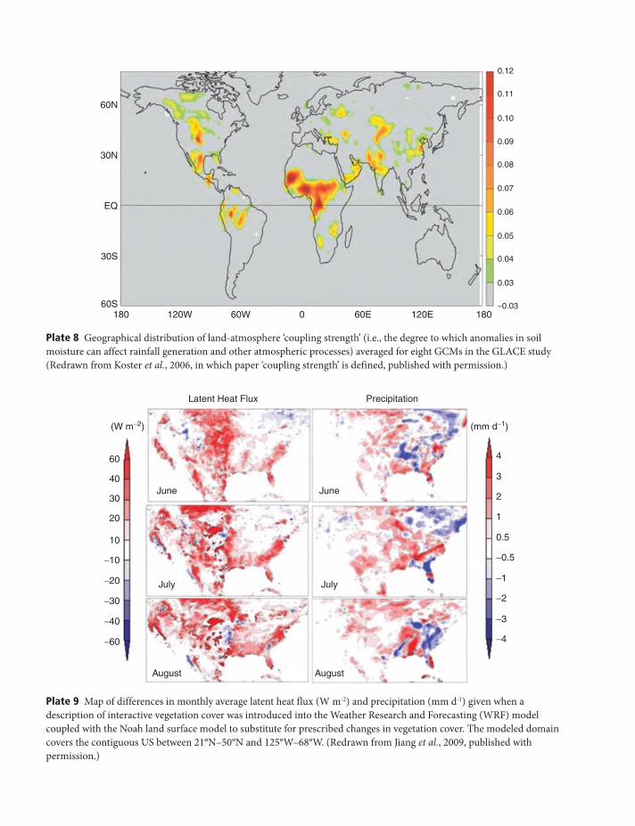
60N
30N
EQ
30S
60S180 120W 60W 0 60E 120E 180
−0.03
0.03
0.04
0.05
0.06
0.07
0.08
0.09
0.10
0.11
0.12
Plate 8 Geographical distribution of land-atmosphere ‘coupling strength’ (i.e., the degree to which anomalies in soil
moisture can affect rainfall generation and other atmospheric processes) averaged for eight GCMs in the GLACE study
(Redrawn from Koster et al., 2006, in which paper ‘coupling strength’ is defined, published with permission.)
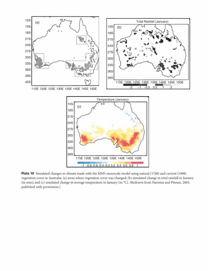
60
(W m−2) (mm d−1)
4
3
2
1
0.5
−0.5
−1
−2
−3
−4
June June
Latent Heat Flux Precipitation
July July
August August
40
30
20
10
−10
−20
−30
−40
−60
Plate 9 Map of differences in monthly average latent heat flux (W m-2) and precipitation (mm d-1) given when a
description of interactive vegetation cover was introduced into the Weather Research and Forecasting (WRF) model
coupled with the Noah land surface model to substitute for prescribed changes in vegetation cover. The modeled domain
covers the contiguous US between 21°N–50°N and 125°W–68°W. (Redrawn from Jiang et al., 2009, published with
permission.)
Shuttleworth_bins.indd 6Shuttleworth_bins.indd 6 11/3/2011 5:39:41 PM11/3/2011 5:39:41 PM
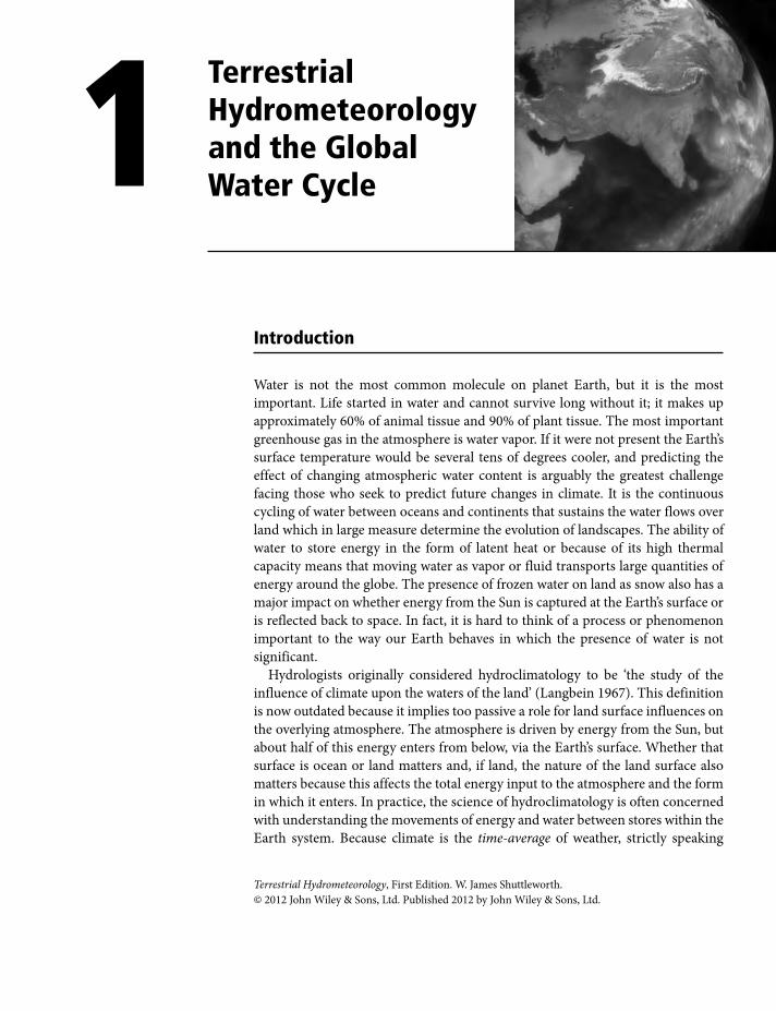
Temperature (January)
(c)
−1 −0.8−0.6−0.4−0.2 0.2 0.4 0.6 0.8 1
115E39S
36S
33S
30S
27S
24S
21S
18S
15S
120E 125E 130E 135E 140E 145E 150E
(a)
42S
39S
36S
33S
30S
27S
24S
21S
18S
15S
12S
115E 120E 125E 130E 135E 140E 145E 150E −3 −1 1 3−0.5 0.5
(b)
39S
36S
33S
30S
27S
24S
21S
18S
15S
115E 120E 125E 130E 135E 140E 145E 150E
Total Rainfall (January)
Plate 10 Simulated changes in climate made with the MM5 mesoscale model using natural (1788) and current (1988)
vegetation cover in Australia: (a) areas where vegetation cover was changed; (b) simulated change in total rainfall in January
(in mm); and (c) simulated change in average temperature in January (in °C). (Redrawn from Narisma and Pitman, 2003,
published with permission.)
Shuttleworth_bins.indd 7Shuttleworth_bins.indd 7 11/3/2011 5:39:44 PM11/3/2011 5:39:44 PM
Terrestrial Hydrometeorology, First Edition. W. James Shuttleworth.
© 2012 John Wiley & Sons, Ltd. Published 2012 by John Wiley & Sons, Ltd.
Introduction
Water is not the most common molecule on planet Earth, but it is the most
important. Life started in water and cannot survive long without it; it makes up
approximately 60% of animal tissue and 90% of plant tissue. The most important
greenhouse gas in the atmosphere is water vapor. If it were not present the Earth’s
surface temperature would be several tens of degrees cooler, and predicting the
effect of changing atmospheric water content is arguably the greatest challenge
facing those who seek to predict future changes in climate. It is the continuous
cycling of water between oceans and continents that sustains the water flows over
land which in large measure determine the evolution of landscapes. The ability of
water to store energy in the form of latent heat or because of its high thermal
capacity means that moving water as vapor or fluid transports large quantities of
energy around the globe. The presence of frozen water on land as snow also has a
major impact on whether energy from the Sun is captured at the Earth’s surface or
is reflected back to space. In fact, it is hard to think of a process or phenomenon
important to the way our Earth behaves in which the presence of water is not
significant.
Hydrologists originally considered hydroclimatology to be ‘the study of the
influence of climate upon the waters of the land’ (Langbein 1967). This definition
is now outdated because it implies too passive a role for land surface influences on
the overlying atmosphere. The atmosphere is driven by energy from the Sun, but
about half of this energy enters from below, via the Earth’s surface. Whether that
surface is ocean or land matters and, if land, the nature of the land surface also
matters because this affects the total energy input to the atmosphere and the form
in which it enters. In practice, the science of hydroclimatology is often concerned
with understanding the movements of energy and water between stores within the
Earth system. Because climate is the time-average of weather, strictly speaking
1 Terrestrial Hydrometeorology and the Global Water Cycle
Shuttleworth_c01.indd 1Shuttleworth_c01.indd 1 11/3/2011 6:35:05 PM11/3/2011 6:35:05 PM
2 TH and the Global Water Cycle
hydroclimatology emphasizes the time-average movement of energy and water.
Such movement occurs in two directions, both out of and into the atmosphere.
Consequently, the present text is motivated not only by the need to understand the
global and regional scale atmospheric features that affect the weather in a specific
catchment, but also to understand how the surface-atmosphere exchanges that
operate inside a catchment contribute along with those from nearby catchments to
determine the subsequent state of the atmosphere downwind.
Broadly speaking, hydrometeorology differs from hydroclimatology in much
the same way that meteorology differs from climatology. Hydrometeorologists
therefore tend to be more interested in activity at shorter time scales than
hydroclimatologists. They are particularly concerned with the physics, mathematics,
and statistics of the processes and phenomena involved in exchanges between
the atmosphere and ground that typically occur over hours or days. Sometimes
these short-term features are described statistically. Hydrometeorologists may, for
example, analyze precipitation data to compute the historical statistics of intense
storms and flood hazards. However, hydrometeorologists are also interested
in seeking basic physical understanding of surface exchanges of water and energy.
This commonly involves the study of processes that act in the vegetation covering
the ground, or the soil and rock beneath the ground, or in lower levels of the
atmosphere where most atmospheric water vapor is found. The present text
includes some description of the statistical approaches used in hydrometeorology
but gives greater prominence to providing an understanding of fundamental
hydrometeorological processes.
Water in the Earth system
Although there have been several studies which have attempted to quantify where
water is to be found across the globe, the magnitude of the Earth’s water reservoirs
and how much water flows between these reservoirs still remains poorly defined.
Table 1.1 gives estimates of the size of the eight main reservoirs together with the
approximate proportion of the entire world’s water stored in each reservoir and
an estimate of the turnover time for the water. The magnitude of the groundwater
reservoir and the associated residence time is complicated by the fact that a large
proportion of the water in this reservoir is ‘fossil water’ stored in deep aquifers
which were created over thousands of years by slow geo-climatic processes. The
amount of such fossil water stored is very difficult to estimate globally. Defining
a residence time for oceans is also complicated. This is because oceans usually
have a fairly shallow layer of surface water on the order of 100 m deep that
interacts comparatively readily with the atmospheric and terrestrial reservoirs,
but this layer overlies a much deeper, slower moving, and more isolated reservoir
of saline water.
Clearly oceans are by far the largest reservoir of water on Earth, which means
that a vast proportion of water on the Earth is salt water. The majority of Earth’s
Shuttleworth_c01.indd 2Shuttleworth_c01.indd 2 11/3/2011 6:35:06 PM11/3/2011 6:35:06 PM
TH and the Global Water Cycle 3
freshwater supply is currently stored in the polar ice caps, as glaciers or permafrost,
or as groundwater. Freshwater lakes, rivers, and marshes contain only about 0.01%
of Earth’s total water. The water present in the atmosphere is very small indeed,
only about 0.001%. However, the water exchanged between this atmospheric
reservoir and the oceanic and land reservoirs is comparatively large, on the order
of 100 km3 per year for land and 400 km3 per year for oceans. Consequently, there
is a rapid turnover in atmospheric water and the atmospheric residence time is
low.
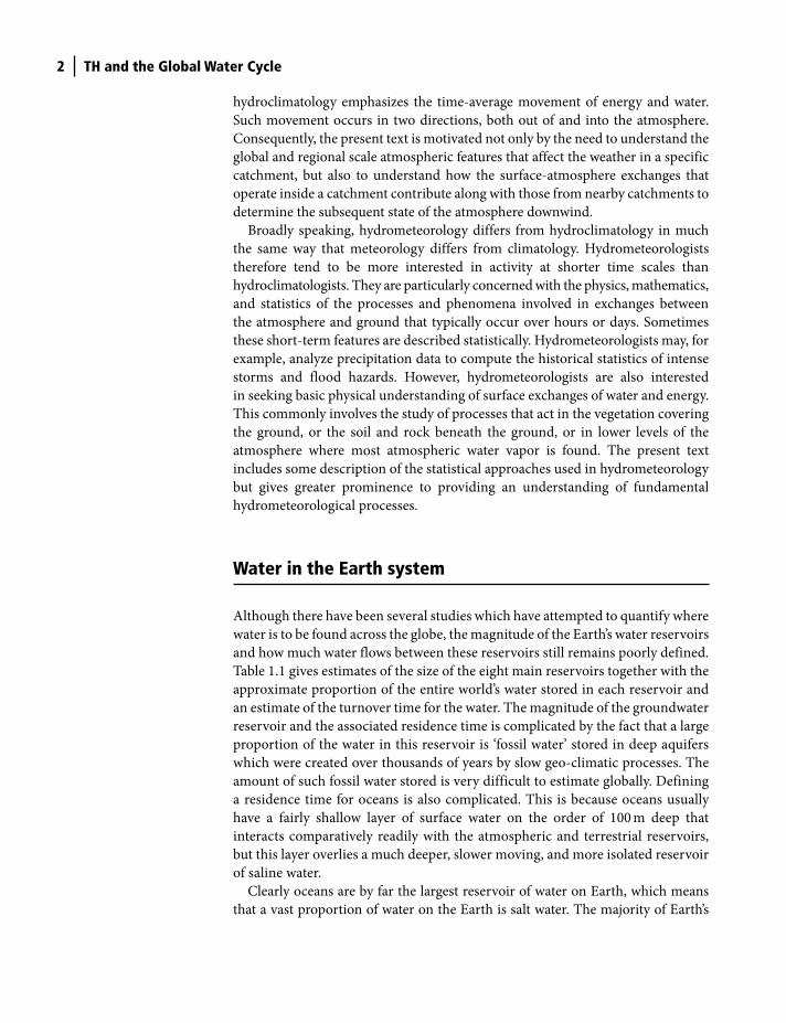
Figure 1.1 illustrates the annual average hydrological cycle for the Earth as a
whole, together with an alternative set of estimates of water stores made by
combining observations with model-calculated data. It is clear that the simple
concept of a hydrological cycle that merely involves water evaporating from the
ocean, falling as precipitation over land then running back to the ocean is a poor
representation of the truth. There are also substantial hydrological cycles over the
oceans which cover about 70% of the globe, and over the continents which cover
the remainder, as well as water exchanged in atmospheric and river flows between
these two.
On average there is a net transfer from oceanic to continental surfaces because
the oceans evaporate about 413 × 103 km3 yr −1 of water, which is equivalent to about
1200 mm of evaporation, but they receive back only about 90% of this as
precipitation. Some of the water evaporated from the ocean is therefore transported
over land and falls as precipitation, but on average about 65% of this terrestrial
precipitation is then re-evaporated and this provides some of the water subsequently
falling as precipitation elsewhere over land. On average about 35% of terrestrial
precipitation returns to the ocean as surface runoff, but the proportion of terrestrial
precipitation that is re-evaporated and the proportion leaving as surface runoff
Table 1.1 Estimated sizes of the main water reservoirs in the Earth system, the
approximate percentage of water stored in them and turnover time of each reservoir
(Data from Shiklomanov, 1993).
Volume (106 km3)
Prcentage of total
Approximate residence time
Oceans (including saline inland seas)
∼1340 ∼96.5 1000 – 10 000 years
Atmosphere ∼0.013 ∼0.001 ∼10 daysLand: Polar Ice, glaciers, permafrost
∼24 ∼1.8 10 – 1000 years
Groundwater ∼23 ∼1.7 15 days – 10 000 yearsLakes, swamps, marshes ∼0.19 0.014 ∼10 yearsSoil moisture ∼0.017 0.001 ∼50 daysRivers ∼0.002 ∼0.0002 ∼15 daysBiological water ∼0.0011 ∼0.0001 ∼10 days
Shuttleworth_c01.indd 3Shuttleworth_c01.indd 3 11/3/2011 6:35:06 PM11/3/2011 6:35:06 PM
4 TH and the Global Water Cycle
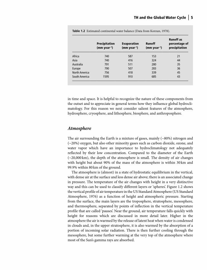
varies significantly both regionally and with season. Area-average runoff in the
semi-arid south western USA is, for example, commonly just a few percent. When
averaged over large continents and over a full year, variations in the fraction of
precipitation leaving as runoff are less. Table 1.2 gives an example of the estimated
annual water balance for the continents (Korzun 1978). Runoff ratios in the range
of 35 to 45% are the norm, but the extensive arid and semi-arid regions of Africa
reduce average runoff for that continent. Fractional runoff in the form of icebergs
from Antarctica is hard to quantify but may be 80% because sublimation from the
snow and ice covered surface is low.
Components of the global hydroclimate system
Understanding the hydroclimate of the Earth does not merely require knowledge
of hydrometeorological process in the atmosphere. Several different components
of the Earth system interact to control the way near-surface weather variables vary
Landprecipition
113
Land
RiversLakes178
Soil moisture122
Ocean
Ocean1 335 040
Surface flow
Ground water flow
Oceanevaporation 413
Oceanprecipitation
373
Ocean to landWater vapor transport
40
Atmosphere12.7
Groundwater15 300
Permafrost22
Vegetation
Percolation
40
Evaporation, transpiration 73
Ice26,350
Figure 1.1 The global annual average hydrological cycle including estimates of the main water reservoirs (in plain font in
units of 103 km3) and of the flow of moisture between stores (in italics in units of 103 km3 yr−1). (From Trenberth et al., 2007,
published with permission.) See Plate 1 for a colour version of this image.
Shuttleworth_c01.indd 4Shuttleworth_c01.indd 4 11/3/2011 6:35:06 PM11/3/2011 6:35:06 PM
TH and the Global Water Cycle 5
in time and space. It is helpful to recognize the nature of these components from
the outset and to appreciate in general terms how they influence global hydrocli-
matology. For this reason we next consider salient features of the atmosphere,
hydrosphere, cryosphere, and lithosphere, biosphere, and anthroposphere.
Atmosphere
The air surrounding the Earth is a mixture of gases, mainly (~80%) nitrogen and
(~20%) oxygen, but also other minority gases such as carbon dioxide, ozone, and
water vapor which have an importance to hydroclimatology not adequately
reflected by their low concentration. Compared to the diameter of the Earth
(~20,000 km), the depth of the atmosphere is small. The density of air changes
with height but about 90% of the mass of the atmosphere is within 30 km and
99.9% within 80 km of the ground.
The atmosphere is (almost) in a state of hydrostatic equilibrium in the vertical,
with dense air at the surface and less dense air above; there is an associated change
in pressure. The temperature of the air changes with height in a very distinctive
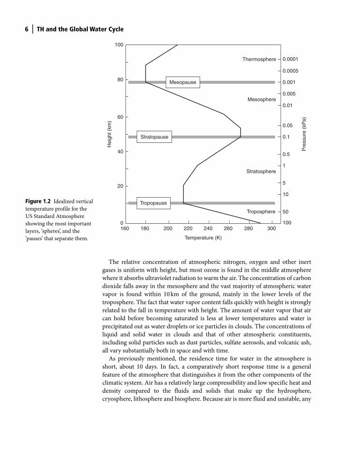
way and this can be used to classify different layers or ‘spheres’. Figure 1.2 shows
the vertical profile of air temperature in the US Standard Atmosphere (US Standard
Atmosphere, 1976) as a function of height and atmospheric pressure. Starting
from the surface, the main layers are the troposphere, stratosphere, mesosphere,
and thermosphere, separated by points of inflection in the vertical temperature
profile that are called ‘pauses’. Near the ground, air temperature falls quickly with
height for reasons which are discussed in more detail later. Higher in the
atmosphere the air is warmed by the release of latent heat when water is condensed
in clouds and, in the upper stratosphere, it is also warmed by the absorption of a
portion of incoming solar radiation. There is then further cooling through the
mesosphere, but some further warming at the very top of the atmosphere where
most of the Sun’s gamma rays are absorbed.
Table 1.2 Estimated continental water balance (Data from Korzun, 1978).
Precipitation (mm year−1)
Evaporation (mm year−1)
Runoff (mm year−1)
Runoff as percentage of precipitation
Africa 740 587 153 21Asia 740 416 324 44Australia 791 511 280 35Europe 790 507 283 36North America 756 418 339 45South America 1595 910 685 43
Shuttleworth_c01.indd 5Shuttleworth_c01.indd 5 11/3/2011 6:35:07 PM11/3/2011 6:35:07 PM
6 TH and the Global Water Cycle
The relative concentration of atmospheric nitrogen, oxygen and other inert
gases is uniform with height, but most ozone is found in the middle atmosphere
where it absorbs ultraviolet radiation to warm the air. The concentration of carbon
dioxide falls away in the mesosphere and the vast majority of atmospheric water
vapor is found within 10 km of the ground, mainly in the lower levels of the
troposphere. The fact that water vapor content falls quickly with height is strongly
related to the fall in temperature with height. The amount of water vapor that air
can hold before becoming saturated is less at lower temperatures and water is
precipitated out as water droplets or ice particles in clouds. The concentrations of
liquid and solid water in clouds and that of other atmospheric constituents,
including solid particles such as dust particles, sulfate aerosols, and volcanic ash,
all vary substantially both in space and with time.
As previously mentioned, the residence time for water in the atmosphere is
short, about 10 days. In fact, a comparatively short response time is a general
feature of the atmosphere that distinguishes it from the other components of the
climatic system. Air has a relatively large compressibility and low specific heat and
density compared to the fluids and solids that make up the hydrosphere,
cryosphere, lithosphere and biosphere. Because air is more fluid and unstable, any
20
40
60
80
100
0160 180 200 220
Temperature (K)
240 260 280 300100
50
10
5
1
0.5
0.1
0.05
0.01
0.005
0.001
0.0005
0.0001Thermosphere
Mesosphere
Mesopause
Stratosphere
Stratopause
Hei
ght (
km)
Pre
ssur
e (k
Pa)
Troposphere
TropopauseFigure 1.2 Idealized vertical
temperature profile for the
US Standard Atmosphere
showing the most important
layers, ‘spheres’, and the
‘pauses’ that separate them.
Shuttleworth_c01.indd 6Shuttleworth_c01.indd 6 11/3/2011 6:35:07 PM11/3/2011 6:35:07 PM

TH and the Global Water Cycle 7
perturbations generated by changes in the inputs that drive the atmosphere
typically decay with time scales on the order of days to weeks.
Differential heating by the Sun causes movement in the atmosphere that is
complicated by the rotation of the Earth, the Earth’s orbit around the Sun, and
inhomogeneous surface conditions. Consequently, the air in the troposphere
undergoes large-scale circulation which, on average, is organized at the global
scale. There are substantial perturbations within this circulation associated with
weather systems at mid-latitudes, and also pseudo-random turbulent motion in
the atmospheric boundary layer and near ‘jet streams’ higher in the atmosphere.
Figure 1.3 shows how contributions to the variance of atmospheric movements in
the atmospheric boundary layer change as a function of frequency. Most movement
occurs at low frequencies. The first peak in this figure is associated with movement
linked to the annual cycle and is in response to seasonal changes in solar heating,
while the third peak is linked to the daily cycle of heating. The large contribution
to variance at the time scales of days to weeks is the result of the large-scale
disturbances associated with transient weather systems. At lower frequencies
atmospheric variance is therefore mainly associated with horizontal features
within the atmospheric circulation. The fourth maximum in variance, which
occurs at timescales of an hour or less, is different because it is due to small-scale
turbulent motions. Such turbulent variations occur in all directions, but their
influence on the vertical movement of atmospheric properties and constituents is
particularly important. Understanding this influence on the vertical movement is
a critical aspect of hydrometeorology.
10
0.01 0.1 1 10
1 day1 month
Frequency (day−1)
Kin
etic
ene
rgy
(m−2
s−2)
1 year
1 hour 1 min. 1 sec.
100 1000 10 000
20
30
40
50
Figure 1.3 Approximate
spectrum of the contributions
to the variance in the
atmosphere for frequencies
between 1 second and 1000
days.
Shuttleworth_c01.indd 7Shuttleworth_c01.indd 7 11/3/2011 6:35:08 PM11/3/2011 6:35:08 PM
8 TH and the Global Water Cycle
Hydrosphere
The liquid water in oceans, interior seas, lakes, rivers, and subterranean waters
constitute the Earth’s hydrosphere. Oceans cover about 70% of the Earth’s surface
and therefore intercept more total solar energy than land surfaces. Most of the
energy leaves oceanic surfaces in the form of latent heat in water vapor, but this is
not necessarily the case for land surfaces. Consequently, maritime air masses are
very different to continental air masses. The atmosphere and oceans are strongly
coupled by the exchange of energy, matter (water vapor), and momentum at their
interface, and precipitation strongly influences ocean salinity. The mass and
specific heat of the water in oceans is much greater than for air and understanding
this difference is very important in the context of seasonal changes in the atmos-
phere. The oceans represent an enormous reservoir for stored energy. As a result,
changes in the sea surface temperature happen fairly slowly and this moderates the
rate of change of associated features in the atmosphere, thereby greatly aiding
seasonal climate prediction.
The oceans are also denser than the atmosphere and have a larger mechanical
inertia, so ocean currents are much slower than atmospheric flows, and oceanic
movement at depth is particularly slow. The atmosphere is heated from below by
the Sun’s energy intercepted by the underlying surface, but oceanic heating is from
above. Consequently, there is a profound difference in the way buoyancy acts in
these two fluid media. The higher temperature at the surface of the sea means
oceanic mixing by surface winds tends to be suppressed, and such mixing is lim-
ited to the active surface layer that has a thickness on the order of 100 m. A strong
gradient of temperature below this surface layer separates it from the deep ocean.
The response time for oceanic movement in the upper mixed layer is weeks to
months to seasons. In the deep ocean, however, movement due to density variations
associated with changes in temperature and salinity occur over time scales from
centuries to millennia. There are eddies in the upper ocean but turbulence is in
general much less pronounced than in the atmosphere. Ocean currents are
important because they move heat from the tropical regions, where incidental
solar radiation is greatest, toward colder mid-latitude and polar regions where
radiation is least. Currents in the upper layer of the ocean are driven by the
prevailing wind patterns in the atmosphere. Ocean flow is from east to west in the
tropics (in response to the trade winds), poleward on the eastern side of continents,
then back toward the equator on the western side of continents.
Lakes, rivers, and subterranean waters make up the remainder of the hydro-
sphere. They can have significant hydrometeorological and hydroclimatological
significance in continental regions, particularly at regional and local scale. The
contrast between the influence on the atmosphere of open water on the one hand
and land surfaces on the other is significant. This is responsible for ‘lake effect’
snowfall in the US Great Lakes and ‘river breeze’ effects near the Amazon River,
for example. River flow into oceans also has an important influence on ocean
salinity near coasts.
Shuttleworth_c01.indd 8Shuttleworth_c01.indd 8 11/3/2011 6:35:08 PM11/3/2011 6:35:08 PM
TH and the Global Water Cycle 9
Cryosphere
The areas of snow and ice, including the extended ice fields of Greenland and
Antarctica, other continental glaciers and snowfields, sea ice, and areas of permafrost,
are the Earth’s cryosphere. The cryosphere has an important influence on climate
because of its high reflectivity to solar radiation. Continental snow cover and sea ice
have a market seasonally, and this can give rise to significant intra-annual and perhaps
interannual variations in the surface energy budgets of frozen polar oceans and conti-
nents with seasonal snow cover. Gradual warming in polar regions has the potential to
give rise to similar changes in surface energy balance over longer time periods. The
low thermal diffusivity of ice can also influence the surface energy balance at high lati-
tudes, because ice acts as an insulator inhibiting loss of heat to the atmosphere from
the underlying water and land. Near-surface cooling also gives rise to stable atmos-
pheres, which inhibit convection and contribute to cooler climates locally.
The large continental ice sheets do not change quickly enough to influence seasonal or interannual climate much, but historical changes in ice sheet extent
and potential changes in the future extent of ice sheets are important because they
are associated with changes in sea level. If substantial melting of the continental ice
sheets occurs, altered sea level could change the boundaries of islands and
continents. Since many inhabited areas are close to such boundaries, sea level
change will likely have serious consequences for human welfare that are dispro-
portionate to the fractional area of land affected. The effect of global warming on
ice sheets is considered a major threat for this reason.
Lithosphere
The lithosphere, which includes the continents and the ocean floor, has an almost
permanent influence on the climatic system. There is large-scale transfer of
angular momentum through the action of torques between the oceans and the
continents. Continental topography affects air motion and global circulation
through the transfer of mass, angular momentum, and sensible heat, and the
dissipation of kinetic energy by friction in the atmospheric boundary layer.
Because the atmosphere is comparatively thin, organized topography in the form
of extended mountain ranges that lie roughly perpendicular to the preferred
atmospheric circulation, such as the Rocky Mountains in North America and the
Andes Mountains in South America, can inhibit how far maritime air penetrates
into continents and thus affect where clouds and precipitation occur.
The transfer of mass between the atmosphere and lithosphere is mainly as water
vapor, rain, and snow. However, this may sometimes also occur as dust when vol-
canoes throw matter into the atmosphere and increase the turbidity of the air. The
ejected sulfur-bearing gases and particulate matter may modify the aerosol load
and radiation balance of the atmosphere and influence climate over extended
areas. The soil moisture in the active layer of the continental lithosphere that is
Shuttleworth_c01.indd 9Shuttleworth_c01.indd 9 11/3/2011 6:35:08 PM11/3/2011 6:35:08 PM
10 TH and the Global Water Cycle
accessible to the atmosphere via plants can have a marked influence on the local
energy balance at the land surface. Soil moisture content affects the rate of
evaporation, the reflection by soil of solar radiation, and the thermal conductivity
of the soil. Because soil moisture tends to change fairly slowly it can provide a
land-based ‘memory’ with an effect on the atmosphere broadly equivalent to that
of slowly changing sea surface temperature.
Biosphere
Terrestrial vegetation, continental fauna, and the flora and fauna of the oceans
make up the biosphere. It is now recognized that the nature of vegetation covering
the ground is not only influenced by the regional hydroclimate, but also itself
influences the hydroclimate of a region. This is because the type of vegetation
present affects the aerodynamic roughness and solar reflectivity of the surface, and
whether water falling as precipitation leaves as evaporation or runoff. The rooting
depth of vegetation matters because it determines the size of the moisture store
available to the atmosphere. Changes in the type of vegetation present may occur
in response to changes in climate, and modern climate prediction models attempt
to represent such evolution. Imposed changes caused by human intervention
through, for example, large-scale deforestation or irrigation also occur and these
can be extensive and alter surface inputs to the atmosphere of continental regions.
The behavior of the biosphere influences the carbon dioxide present in the
atmosphere and oceans through photosynthesis and respiration. It is essential to
include description of these influences when models are used to simulate global
warming. For this reason, advanced sub-models describing the biosphere in mete-
orological models seek to represent the energy, water, and carbon exchanges of the
biosphere simultaneously. Water and carbon exchanges are linked by the fact that
the water transpired and the carbon assimilated by vegetation occurs by molecular
diffusion through the same plant stomata. Models of the biosphere are often
referred to as Land Surface Parameterization Schemes (LSPs) or Soil Vegetation
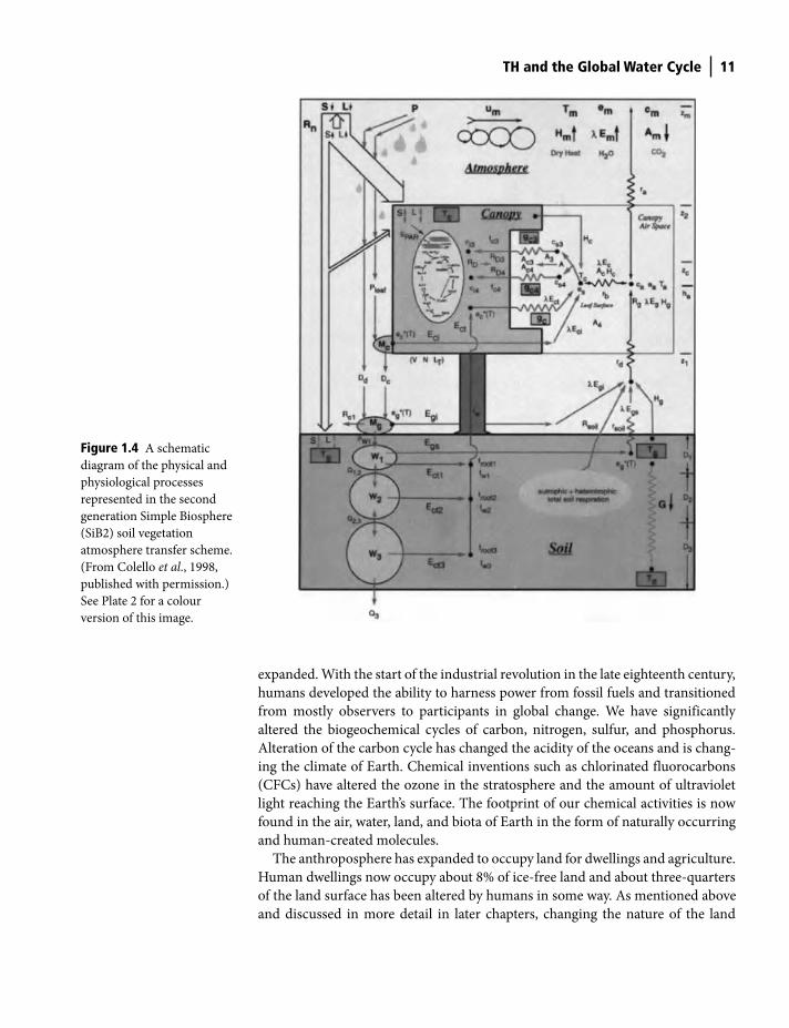
Atmosphere Transfer Schemes (SVATs); see Chapter 24 for greater detail. Figure 1.4
shows an example of the Simple Biosphere Model (SiB; Sellers et al., 1986), an
example of a SVAT that is currently widely used.
Because the biosphere is sensitive to changes in climate, detailed study of past
changes in its nature and behavior as revealed in fossils and tree rings and in pollen
and coral records is important as a means of documenting the prevailing climate
in previous eras.
Anthroposphere
The word anthroposphere is used to describe the effect of human beings on the
Earth system. For much of our existence human impact on the environment was
small, but as our numbers grew our impact on the atmosphere and landscape
Shuttleworth_c01.indd 10Shuttleworth_c01.indd 10 11/3/2011 6:35:08 PM11/3/2011 6:35:08 PM
TH and the Global Water Cycle 11
expanded. With the start of the industrial revolution in the late eighteenth century,
humans developed the ability to harness power from fossil fuels and transitioned
from mostly observers to participants in global change. We have significantly
altered the biogeochemical cycles of carbon, nitrogen, sulfur, and phosphorus.
Alteration of the carbon cycle has changed the acidity of the oceans and is chang-
ing the climate of Earth. Chemical inventions such as chlorinated fluorocarbons
(CFCs) have altered the ozone in the stratosphere and the amount of ultraviolet
light reaching the Earth’s surface. The footprint of our chemical activities is now
found in the air, water, land, and biota of Earth in the form of naturally occurring
and human-created molecules.
The anthroposphere has expanded to occupy land for dwellings and agriculture.
Human dwellings now occupy about 8% of ice-free land and about three-quarters
of the land surface has been altered by humans in some way. As mentioned above
and discussed in more detail in later chapters, changing the nature of the land
Figure 1.4 A schematic
diagram of the physical and
physiological processes
represented in the second
generation Simple Biosphere
(SiB2) soil vegetation
atmosphere transfer scheme.
(From Colello et al., 1998,
published with permission.)
See Plate 2 for a colour
version of this image.
Shuttleworth_c01.indd 11Shuttleworth_c01.indd 11 11/3/2011 6:35:08 PM11/3/2011 6:35:08 PM
12 TH and the Global Water Cycle
surface is important for hydrometeorology because it alters the way energy from
the Sun enters the atmosphere from below and, if sufficiently extensive, land-use
change has impact on regional and perhaps global climate and weather. Examples
of such change include urban heat islands and changes to regional evaporation due
to the building of large dams, extensive irrigation, and land-cover change such as
deforestation.
When compared with most natural changes in other spheres of the globe,
change in the anthroposphere is happening very rapidly. This is partly because
human population has increased quickly over the past few centuries and still is
today, but also because strides in technology have empowered humans to
directly and indirectly effect change to the environment in new and different
ways, and because as society develops the per capita demand for energy
increases hugely.
Important points in this chapter
● Hydrometeorology: hydrometeorology (and this text) concerns the physics,
mathematics, and statistics of processes and phenomena involved in
exchanges between the atmosphere and ground that typically occur over
hours or days, and how the time average of these exchanges combine to
define hydroclimatology.
● Water reservoirs: the size of the Earth’s water reservoirs are poorly defined
but include the oceans (~ 95.6%), groundwater (~2.4%), frozen water (1.9%),
and water bodies, soil moisture, atmospheric water, rivers and biological
water (in total ~ 0.01%).
● Water cycle: as a global average about 90% of oceanic evaporation falls back
to the oceans as precipitation, the remainder being transported over land;
and about 55–65% of the precipitation falling over land re-evaporates
(depending on the continent) leaving 35–45% to runoff back to the ocean in
rivers and icebergs.
● Atmosphere:
— Constituents and structure: About 80% N2 and 20% O
2 and other minority
gases (CO2, O
3, H
2O, etc.), 99.9% of which are within 80 km of the ground
in the troposphere, stratosphere, mesosphere, thermosphere, with most
water vapor in the lower troposphere within 10 km of the ground.
— Circulation: Differential heating by the Sun causes global circulation in
the troposphere which moves energy toward the poles and which is
complicated by the Coriolis force but is, on average, organized.
— Variance: Contributions to the variance of the atmosphere arise at
frequencies linked to the seasonal cycle, transient weather systems,
and the daily cycle, with these contributions separated by a distinct
spectral gap from those at higher frequencies that are associated
with turbulence.
Shuttleworth_c01.indd 12Shuttleworth_c01.indd 12 11/3/2011 6:35:09 PM11/3/2011 6:35:09 PM
TH and the Global Water Cycle 13
● Hydrosphere:
— Extent and importance: Oceans cover ~70% of the Earth and the solar
energy they intercept is mainly used to evaporate water vapor into the
atmosphere; they have a large thermal capacity and act as ‘memory’ in the
Earth system that influences season climate.
— Structure: Oceans have a surface layer 10s–100s m deep warmed by the
Sun’s energy in which there are wind-driven ocean currents, this layer
being separated by a strong thermal gradient from the deep ocean which
moves very slowly in response to changes in temperature and salinity.
— Currents: Upper ocean currents move heat from the tropics to polar
regions: ocean flow is east to west in the tropics, poleward on the eastern
side of continents, then back toward the equator on the western side of
continents.
● Cryosphere: comprises the polar ice fields and glaciers that change slowly
and transient continental snow/ice fields with a strong seasonal influence on
climate.
● Lithosphere: organized topography perpendicular to atmospheric flow can
inhibit penetration of maritime air into continents, and aerosols from volca-
noes can alter the radiation balance over extensive areas.
● Biosphere: vegetation cover affects aerodynamic roughness and reflection of
solar energy and by intercepting rainfall and accessing water in the soil
through roots, also whether precipitation leaves as evaporation or runoff.
● Anthroposphere: human population is now large enough to influence cli-
mate, mainly by changing the concentrations of gases in the atmosphere and
by modifying land cover over large areas.
References
Colello, G.D., Grivet, C., Sellers, P.J., & Berry, J.A. (1998) Modeling of energy, water, and
CO2 flux in a temperate grassland ecosystem with SiB2: May–October 1987. Journal of
Atmospheric Sciences, 55 (7), 1141–69.
Langbein, W.G. (1967) Hydroclimate. In: The Encyclopaedia of Atmospheric Sciences and
Astrogeology (ed. R.W. Fairbridge), pp. 447–51. Reinhold, New York.
Korzun, V.I. (1978) World Water Balance of the Earth. Studies and Reports in Hydrology, 25.
UNESCO, Paris.
Sellers, P.J., Mintz, Y., Sud, Y.C. & Dalcher, A. (1986) A simple biosphere model (SiB) for use
within general circulation models. Journal of Atmospheric Sciences, 43, 505–531.
Shiklomanov, J.A. (1993) World fresh water resources. In: Water in Crisis: A Guide to the
World’s Fresh Water Resources (ed. P.H. Gleick), pp. 13–24. Oxford University Press, New
York.
Trenberth, K.E., Smith, L., Qian, T., Dai, A. & Fasullo, J. (2007) Estimates of the global water
budget and its annual cycle using observational and model data. Journal of
Hydrometeorology, 8, 758–69.
US Standard Atmosphere (1976) US Government Printing Office, Washington, DC.
Shuttleworth_c01.indd 13Shuttleworth_c01.indd 13 11/3/2011 6:35:09 PM11/3/2011 6:35:09 PM
Water Vapor in the Atmosphere2
Introduction
Hydrometeorologists are commonly concerned with quantifying the amount of
water in the atmosphere in vapor, liquid, and solid form and with seeking to
describe the way energy and water move vertically in the atmosphere toward and
away from the ground. In this chapter we consider the basic definitions and
important concepts needed for this.
Latent heat
The molecules that make up ice are held rigidly together in close proximity by
intermolecular forces. In liquid water the molecules are also close together but,
because they are at a higher temperature, they move around and their average
separation is therefore somewhat greater. In water vapor, molecular separation is
very much larger: molecules in water vapor are typically separated by about ten
molecular diameters. As water molecules move farther apart, the forces that bind
them reduce quickly with distance and at ten molecular diameters these forces are
much smaller than when the molecules are in near contact. Viewed in this way, the
transition from ice to liquid water and then to water vapor can be viewed as a
temperature related increase in the separation of molecules in the face of the
attractive intermolecular forces acting between them.
To move against a force requires work, and therefore energy has to be given to
separate water molecules to give changes in phase. The amount of energy needed
is directly related to the number of molecules present and therefore to the mass of
water that changes phase. The amount of energy needed for ice-to-liquid water
transition is called the latent heat of fusion and is 0.333 MJ kg−1. Because the change
Terrestrial Hydrometeorology, First Edition. W. James Shuttleworth.
© 2012 John Wiley & Sons, Ltd. Published 2012 by John Wiley & Sons, Ltd.
Shuttleworth_c02.indd 14Shuttleworth_c02.indd 14 11/3/2011 6:34:31 PM11/3/2011 6:34:31 PM
Water Vapor in the Atmosphere 15
in separation for transition from liquid water to water vapor is much larger, the
latent heat of vaporization for liquid water is also greater. The amount of energy
needed also depends on the temperature at which the phase changes occur.
Molecules in warm water are already a little farther apart than in cold water, so
rather less energy is needed and the latent heat of vaporization is slightly lower at
higher temperatures. For this reason, l, the latent heat of vaporization of water,
is temperature dependent and when the temperature, TC, is given in °C, l is
calculated by:
−= − 12.501 0.002361 MJ kgCTl
(2.1)
Atmospheric water vapor content
As discussed in Chapter 1, the atmosphere is a complex mixture of gases with
nitrogen and oxygen being the dominant constituents. However, in the tropo-
sphere, water vapor is a particularly important constituent, with a variable con-
centration that is typically a few percent. When describing the concentration of
water vapor in the air, it is convenient to speak in terms of air comprising just
two constituents, i.e., water vapor and ‘dry air.’ Dry air is the general description
of all the other gases present. The sum of these two constituents is then referred
to as ‘moist air.’
If the densities of water vapor, dry air, and moist air in an air sample are rv, r
d
and ra, respectively, the proportion of water vapor in the moist air can be charac-
terized in several different ways. One is as the mixing ratio, r, which is defined as
the ratio of the mass of water vapor to the mass of dry air in the moist air sample,
expressed in terms of densities as:
v
d
r =rr
(2.2)
Another common way to define the water vapor content of an air sample is as the
ratio of the mass of water vapor to the mass of moist air. This ratio, q, is called the
specific humidity of the air, expressed in terms of densities as:
( )v v
a v d
q = =+
r rr r r
(2.3)
Because rv is always considerably less than r
d and r
a, the numerical values of mix-
ing ratio and specific humidity are usually very similar. Strictly speaking, both
r and q are dimensionless quantities, but often q is referred to as having units of
kg kg−1 or, more often, gm kg−1. The specific humidity of air in the troposphere is
generally in the range 0–30 gm kg−1.
Shuttleworth_c02.indd 15Shuttleworth_c02.indd 15 11/3/2011 6:34:32 PM11/3/2011 6:34:32 PM
16 Water Vapor in the Atmosphere
Ideal Gas Law
In the seventeenth and eighteenth centuries it was discovered that there are simple
relationships between the pressure, volume, and temperature of gases. Boyle’s Law,
for example, states that at constant temperature, the absolute pressure, P, and the
volume, V, of a gas are inversely proportional. Similarly, Charles’s Law states that at
constant pressure, the volume of a given mass of an ideal gas increases or decreases
by the same factor as its temperature increases or decreases, providing the
temperature, T, is measured in K. These two laws can be combined to give the
Ideal Gas Law, which has the form:
PV nRT= (2.4)
where R is the universal gas constant equal to 8.314 J mol−1 K−1, and n is the number
of moles of gas considered. One mole of gas is defined as comprising 6.02 × 10²³
molecules: this number is called Avogadro’s number. Strictly speaking, Equation
(2.4) only applies for an ‘ideal’ gas in which the molecules are treated as non-
interacting point particles engaged in a random motion that obeys the conserva-
tion of energy. In practice, however, the real gases that make up the atmosphere
approximate the behavior of an ideal gas closely for the range of temperatures and
pressure found in the troposphere.
The mass of a mole of one specific gas, Mg, is called the gram molecular weight
of the gas. If a volume, V, contains n moles of gas, it therefore has a mass (nMg),
and the sample of gas has a density rg = (nM
g)/V. This means Equation (2.4) can be
re-written as:
g gP R T= r
(2.5)
where Rg = (R/M
g) is the gas constant for the specific gas. It is convenient to use this
second form of the ideal gas law when describing moist air. The gram molecular
weight of water is 18 grams per mole and if dry air is assumed to comprise
78% nitrogen and 22% oxygen, the gram molecular weight of dry air is 29 grams
per mole. Consequently, the specific gas constants of water vapor and dry air are
461.5 J kg−1 K−1 and 286.9 J kg−1 K−1, respectively.
Since the molecules making up a gas are typically separated by about ten
molecular diameters at normal temperatures and pressures, only about one
thousandth of the volume of the gas is actually occupied by gas molecules. Gases
are therefore largely empty space and this means that for a gas that is a mixture of
molecules, the contribution to the pressure made by one constituent gas in the
mixture is independent of the pressure contribution made by the other gases
present. This result is Dalton’s law of partial pressures, and it means that the ideal
gas law can be applied not only to the mixture of gases but also separately to each
constituent in a gas mixture.
Shuttleworth_c02.indd 16Shuttleworth_c02.indd 16 11/3/2011 6:34:35 PM11/3/2011 6:34:35 PM
Water Vapor in the Atmosphere 17
Thus, if a sample of moist air has a total pressure, P, the contribution to that
pressure given by the water vapor molecules it contains, e, called the vapor pressure
of the moist air, is given by:
v ve R T= r
(2.6)
where rv is the (variable) density of the water vapor in the moist air mixture and R
v
is the gas constant for water vapor. Similarly, if we treat the remainder of the moist
air as being one gas, the contribution to the total pressure of this dry air compo-
nent of the moist air gas mixture is (P-e), given by:
( ) ( )a v dP e R T− = −r r
(2.7)
where ra is the density of the moist air mixture and R
d is the gas constant of the dry
air. Like the mixing ratio and specific humidity, the vapor pressure of the air is a
measure of the amount of water vapor present in a sample of moist air and it is
frequently used as such in this text.
The different measures of atmospheric water vapor content are of course inter-
related. Because (Rd /R
v) = 0.62, the relationship between the specific humidity and
vapor pressure of the air can be shown to have the form:
( )( )
0.62
0.381
d vv
a d v
e R R eq
P eP e R R= = =
−⎡ ⎤− −⎣ ⎦
rr
(2.8)
with q in kg kg−1. However, because e is usually much less than P it is often accept-
able to assume that, to an accuracy of a few percent:
0.622e
q rP
= =
(2.9)
Virtual temperature
Combining Equations (2.6) and (2.7) gives:
( ) 1 1v v
a v d v v a d
d a
RP R T R T R T
R
⎡ ⎤⎛ ⎞= − + = + −⎢ ⎥⎜ ⎟⎝ ⎠⎢ ⎥⎣ ⎦
rr r r r
r
(2.10)
This equation can be re-written as:
a d vP R T= r
(2.11)
Shuttleworth_c02.indd 17Shuttleworth_c02.indd 17 11/3/2011 6:34:37 PM11/3/2011 6:34:37 PM
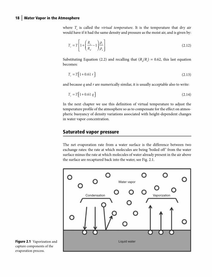
18 Water Vapor in the Atmosphere
where Tv is called the virtual temperature. It is the temperature that dry air
would have if it had the same density and pressure as the moist air, and is given by:
1 1v v
v
d a
RT T
R
⎡ ⎤⎛ ⎞= + −⎢ ⎥⎜ ⎟⎝ ⎠⎢ ⎥⎣ ⎦
rr
(2.12)
Substituting Equation (2.2) and recalling that (Rd/R
v) = 0.62, this last equation
becomes:
1 0.61 v
T T r= +⎡ ⎤⎣ ⎦ (2.13)
and because q and r are numerically similar, it is usually acceptable also to write:
1 0.61 v
T T q= +⎡ ⎤⎣ ⎦ (2.14)
In the next chapter we use this definition of virtual temperature to adjust the
temperature profile of the atmosphere so as to compensate for the effect on atmos-
pheric buoyancy of density variations associated with height-dependent changes
in water vapor concentration.
Saturated vapor pressure
The net evaporation rate from a water surface is the difference between two
exchange rates: the rate at which molecules are being ‘boiled off ’ from the water
surface minus the rate at which molecules of water already present in the air above
the surface are recaptured back into the water, see Fig. 2.1.
Condensation Vaporization
Water vapor
Liquid waterFigure 2.1 Vaporization and
capture components of the
evaporation process.
Shuttleworth_c02.indd 18Shuttleworth_c02.indd 18 11/3/2011 6:34:42 PM11/3/2011 6:34:42 PM

Water Vapor in the Atmosphere 19
According to Kevin-Boltzmann statistics, the number of molecules that acquire
enough energy to break the intermolecular bonds in the water and enter the over-
lying air is related to temperature, i.e.:
1“Boil off ” rate exp
nk
kT
⎛ ⎞≈ −⎜ ⎟⎝ ⎠
l
(2.15)
where k and k1 are constants and n is the number of molecules per unit volume.
On the other hand, the rate of capture of molecules is directly related to concentra-
tion of vapor molecules in the overlying air, i.e.:
( )2“Capture” rate 1 'k r e≈ −
(2.16)
where k2 is a constant and r′ is the fraction of water vapor molecules colliding with
the surface that are reflected without capture. If the (temperature dependent) boil
off rate exceeds the (concentration dependent) capture rate, there is net evapora-
tion and liquid water leaves the surface and enters the air as water vapor.
But what would happen if the air above the evaporating water surface was enclosed
so that evaporated molecules were not able to diffuse away higher into the atmos-
phere? Gradually the concentration of molecules in the air would rise until such time
as the rate of capture equaled the rate of boil off. There would then be no net loss of
water molecules, evaporation would cease; the air is then be said to be saturated.
Because net evaporation is the difference between two rates, there is a well-defined
concentration of water vapor at which the net exchange is zero. This concentration
depends on the temperature-dependent boil off rate. Were the temperature higher,
for example, the boil off rate would increase and exchange equilibrium would be
established with the saturated air having a higher concentration of water vapor.
The relationship between the saturated vapor pressure, esat
, and temperature has
been defined by experiment and several empirically determined relationships
have been proposed. Here we select the following:
⎛ ⎞= ⎜ ⎟+⎝ ⎠
17.27 0.6108exp kPa
237.3
C
sat C
Te
T
(2.17)
when the temperature is given in °C. Note that elsewhere in this text the temperature,
T, is usually expressed in K. Here, T C is used to represent temperature to emphasize
that in this empirical formula the value of temperature must be expressed in °C.
The gradient of the relationship between saturated vapor pressure and temperature
is often used in equations describing evaporation rate and, when used in this way,
this gradient is usually represented by Δ. Differentiating Equation (2.17) gives:
( )1
2
4098 kPa °C
237.3
sat sat
CC
de e
dT T
−Δ = =+
(2.18)
Shuttleworth_c02.indd 19Shuttleworth_c02.indd 19 11/3/2011 6:34:45 PM11/3/2011 6:34:45 PM

20 Water Vapor in the Atmosphere
Figure 2.2 illustrates how esat
and Δ change as a functions of TC. Both variables
change substantially over the normal range of temperatures. The fact that esat
and
Δ have specified relationships with temperature is very important in hydrometeor-
ology: it means that additional equations are available to link the surface exchanges
of water vapor and heat.
At a particular temperature, the density of water vapor in saturated air, rv,sat
, can
be specified from the saturated vapor pressure using Equation (2.6). Consequently,
corresponding values of saturated mixing ratio, rsat
, and saturated specific humid-
ity, qsat
, can be defined by substituting this value of rv,sat
into Equations (2.2) and
(2.3), respectively.
Measures of saturation
Figure 2.3 is helpful, not only because it defines the extent to which the atmosphere
is saturated, but also because later it is used in important methods to measure
the vapor pressure of moist air. This diagram is for the example case of an atmos-
phere with a temperature of 35°C that is 60% saturated.
Probably the most common way to specify the extent to which air is saturated is
to specify its relative humidity, RH. Relative humidity is defined as the ratio of the
actual vapor pressure of the air to the saturation vapor pressure at air temperature
and is normally expressed as a percentage. To good accuracy the relative humidity
can also be calculated as the ratio of the mixing ratio of the air to saturation mixing
ratio at air temperature, or as the ratio of specific humidity of the air to the satura-
tion specific humidity at air temperature, thus:
100 % 100 % 100 %sat sat sat
qe rRH
e r q
⎛ ⎞ ⎛ ⎞ ⎛ ⎞= = =⎜ ⎟ ⎜ ⎟ ⎜ ⎟
⎝ ⎠ ⎝ ⎠ ⎝ ⎠ (2.19)
A second important measure of atmospheric humidity content is the vapor pressure
deficit, D. The vapor pressure deficit is defined as the difference between saturation
vapor pressure at air temperature and the vapor pressure of the air, i.e.:
8
6
4
2
0
0.5
0.4
0.3
0.2
0.1
0.00 10 20
T c �C
30 400 10 20
T c �C
30 40e sat
(kP
a)
Δ (k
Pa�
C– 1
)
Figure 2.2 Variation in
saturated vapor pressure of water
and the gradient of that variation
as a function of temperature
in °C.
Shuttleworth_c02.indd 20Shuttleworth_c02.indd 20 11/3/2011 6:34:49 PM11/3/2011 6:34:49 PM
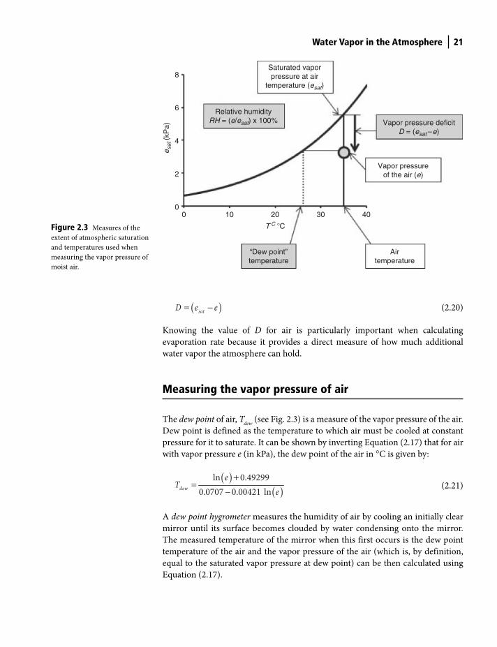
Water Vapor in the Atmosphere 21
( )satD e e= −
(2.20)
Knowing the value of D for air is particularly important when calculating
evaporation rate because it provides a direct measure of how much additional
water vapor the atmosphere can hold.
Measuring the vapor pressure of air
The dew point of air, Tdew
(see Fig. 2.3) is a measure of the vapor pressure of the air.
Dew point is defined as the temperature to which air must be cooled at constant
pressure for it to saturate. It can be shown by inverting Equation (2.17) that for air
with vapor pressure e (in kPa), the dew point of the air in °C is given by:
( )( )
ln 0.49299
0.0707 0.00421 lndew
eT
e
+=
−
(2.21)
A dew point hygrometer measures the humidity of air by cooling an initially clear
mirror until its surface becomes clouded by water condensing onto the mirror.
The measured temperature of the mirror when this first occurs is the dew point
temperature of the air and the vapor pressure of the air (which is, by definition,
equal to the saturated vapor pressure at dew point) can be then calculated using
Equation (2.17).
8
6
4
2
00 10 20
T C �C
30 40
Vapor pressureof the air (e)
Vapor pressure deficitD = (esat– e)
Saturated vaporpressure at air
temperature (esat)
Relative humidityRH = (e/esat) x 100%
Airtemperature
e sat
(kP
a)
“Dew point”temperature
Figure 2.3 Measures of the
extent of atmospheric saturation
and temperatures used when
measuring the vapor pressure of
moist air.
Shuttleworth_c02.indd 21Shuttleworth_c02.indd 21 11/3/2011 6:34:50 PM11/3/2011 6:34:50 PM
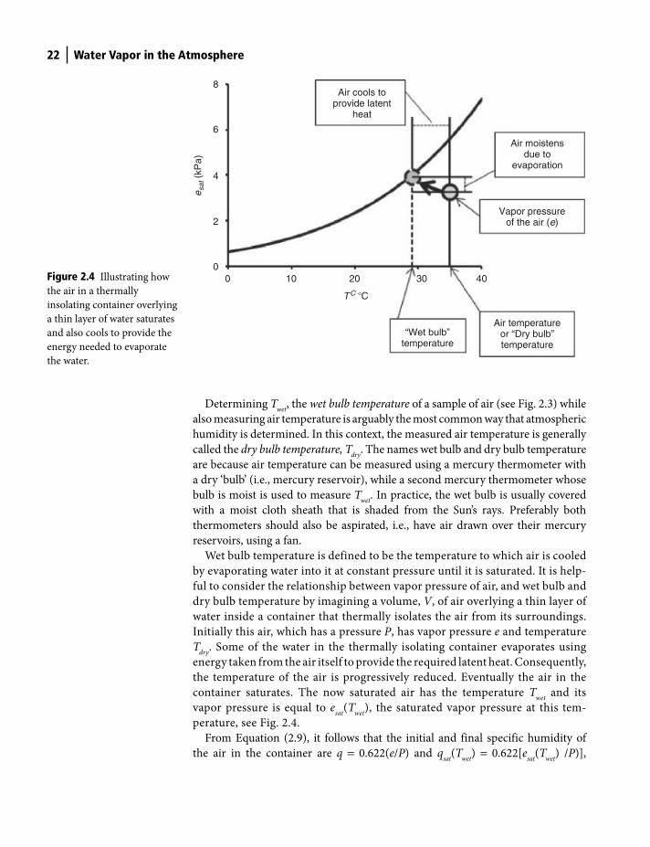
22 Water Vapor in the Atmosphere
Determining Twet
, the wet bulb temperature of a sample of air (see Fig. 2.3) while
also measuring air temperature is arguably the most common way that atmospheric
humidity is determined. In this context, the measured air temperature is generally
called the dry bulb temperature, Tdry
. The names wet bulb and dry bulb temperature
are because air temperature can be measured using a mercury thermometer with
a dry ‘bulb’ (i.e., mercury reservoir), while a second mercury thermometer whose
bulb is moist is used to measure Twet
. In practice, the wet bulb is usually covered
with a moist cloth sheath that is shaded from the Sun’s rays. Preferably both
thermometers should also be aspirated, i.e., have air drawn over their mercury
reservoirs, using a fan.
Wet bulb temperature is defined to be the temperature to which air is cooled
by evaporating water into it at constant pressure until it is saturated. It is help-
ful to consider the relationship between vapor pressure of air, and wet bulb and
dry bulb temperature by imagining a volume, V, of air overlying a thin layer of
water inside a container that thermally isolates the air from its surroundings.
Initially this air, which has a pressure P, has vapor pressure e and temperature
Tdry
. Some of the water in the thermally isolating container evaporates using
energy taken from the air itself to provide the required latent heat. Consequently,
the temperature of the air is progressively reduced. Eventually the air in the
container saturates. The now saturated air has the temperature Twet
and its
vapor pressure is equal to esat
(Twet
), the saturated vapor pressure at this tem-
perature, see Fig. 2.4.
From Equation (2.9), it follows that the initial and final specific humidity of
the air in the container are q = 0.622(e/P) and qsat
(Twet
) = 0.622[esat
(Twet
) /P)],
Air cools toprovide latent
heat
Vapor pressureof the air (e)
Air temperatureor “Dry bulb”temperature
Air moistensdue to
evaporation
“Wet bulb”temperature
403020100
TC �C
8
6
4
2
0
e sat
(kP
a)
Figure 2.4 Illustrating how
the air in a thermally
insolating container overlying
a thin layer of water saturates
and also cools to provide the
energy needed to evaporate
the water.
Shuttleworth_c02.indd 22Shuttleworth_c02.indd 22 11/3/2011 6:34:52 PM11/3/2011 6:34:52 PM

Water Vapor in the Atmosphere 23
respectively. Because the air in the container is thermally isolated, the heat removed
from the air as it cools must equal the latent heat required to evaporate water to
raise the specific humidity of the air to saturation, i.e.:
( ) ( )– – a dry wet p a sat wetV T T c q T q V⎡ ⎤= ⎣ ⎦r r l
(2.22)
where cp (= 1.013 kJ kg−1 K−1) is the specific heat at constant pressure for air.
Rewriting Equation (2.22) in terms of vapor pressure:
( ) ( )0.622 – –
a sat wet
a p dry wet
e T ec T T
P
⎡ ⎤⎣ ⎦=r l
r
(2.23)
This last equation can be re-written as the so-called wet bulb equation, which takes
the form:
( ) ( )– sat wet dry wet
e e T T T= − γ
(2.24)
In this last equation the term (Tdry
– Twet
) is often called the wet bulb depression and
γ is the psychrometric constant calculated from:
0.622
pc P⎛ ⎞
γ = ⎜ ⎟⎝ ⎠l
(2.25)
Actually the psychrometric ‘constant’ is not constant because it varies with
atmospheric pressure and also to some extent with temperature, because the latent
heat of vaporization of water has temperature dependency, see Equation (2.1). For
a temperature of 20°C and pressure of 101.2 kPa, the value of γ is 0.0677.
Wet and dry bulb temperatures are often routinely measured at climate stations
and if measured using aspirated thermometers the value of γ calculated by
Equation (2.25) should be used to calculate the vapor pressure. However, if the
thermometers are not aspirated (which is often the case), a different, empirically
determined value of γ * is required to substitute for γ when calculating the atmos-
pheric vapor pressure from the wet bulb equation.
Important points in this chapter
● Latent heat: separating water molecules in liquid water to give water vapor
requires energy (∼2.5 MJ kg−1) which is called the latent heat of vaporization
and which reduces with temperature by about 0.1% per °C.
● Atmospheric water content: is quantified in terms of the ratio of the density
of water vapor to that of the (dry) air, called the mixing ratio (r), or the
Shuttleworth_c02.indd 23Shuttleworth_c02.indd 23 11/3/2011 6:34:53 PM11/3/2011 6:34:53 PM
24 Water Vapor in the Atmosphere
ratio of the density of water vapor to that of moist air, called the specific
humidity (q). The vapor pressure of air (e) is also a measure of atmospheric
water content.
● Ideal gas law: the temperature (T), volume (V) and pressure (P) of a gas
are related by the ideal gas law which can be written as PV = rgR
gT where
rg and R
g = R/M
g are the density and (gas-specific) gas constant, respectively,
and Mg is its gram molecular weight. When applied to both the dry air and
water vapor portions of moist air, to good accuracy this gives the result
q = r = (0.622 e/P).
● Virtual temperature: Tv = T(1+0.61q) is the temperature that dry air would
have if it had the same density and temperature as the moist air.
● Saturated vapor pressure: the maximum vapor pressure of air when
saturated, esat
, and the rate of change of esat
with temperature, Δ, are both
well-defined functions of the temperature.
● Measures of saturation: two measures in common use are the relative
humidity, RH = (100e)/ esat
, and the vapor pressure deficit D = (esat
– e).
● Measuring the vapor pressure: two ways to measure vapor pressure are:
— Dew point hygrometer: Dew point is obtained as the temperature of an
initially clear mirror cooled until its surface becomes clouded by dew.
Equation (2.17) is then applied to calculate e from Tdew
.
— Wet bulb psychrometer: Two (preferably aspirated) thermometers, one
dry and one wet, measure the dry bulb and wet bulb temperatures,
Tdry
and Twet
, respectively; vapor pressure is calculated from e = esat
( Twet
) –
γ (Tdry
– Twet
) where esat
(Tw) is the saturated vapor pressure at wet bulb tem-
perature and γ is the psychrometric constant.
Shuttleworth_c02.indd 24Shuttleworth_c02.indd 24 11/3/2011 6:34:57 PM11/3/2011 6:34:57 PM
Vertical Gradients in the Atmosphere3
Introduction
Air nearer to the ground must support the column of air above it and so has to
exert an upward force per unit surface area (i.e., an upward pressure) that is equal
and opposite to the downward gravitational force exerted by all the overlying air.
Because the mass of overlying air reduces with distance from the ground, air pres-
sure reduces with height. Air temperature is related to pressure and density
through the ideal gas law, Equation (2.5), so air temperature necessarily also
changes with height. In the absence of any disturbing influences such as heat
inputs from the Sun or surface, the atmosphere would therefore settle into a stable
condition with hydrostatic vertical gradients of pressure, density, and temperature,
all of which can be calculated.
Heat flow occurs when there is non-uniformity in the spatial distribution of
heat in a medium, with movement away from regions with higher temperature
toward regions with lower temperature. But the temperature gradient that is
established in a hydrostatic atmosphere is not associated with vertical heat flow.
Rather it is deviations from this temperature gradient that are associated with the
vertical movement of heat. Consequently, it is convenient to define a variable
that is directly related to vertical heat flow, potential temperature, which is a
combination of both local temperature and pressure, and to calculate the vertical
profile of this potential temperature to diagnose the thermal stability of the
atmosphere.
Because the gram molecular weight of water vapor is less than the average
gram molecular weight of the other gases (mainly nitrogen and oxygen) that
make up air, the density of air with more water vapor is less than that of air with
less water vapor. The concentration of atmospheric water vapor can change with
height, and height dependent variations in density associated with changes in
fractional vapor content complicate the relationship between the density,
Terrestrial Hydrometeorology, First Edition. W. James Shuttleworth.
© 2012 John Wiley & Sons, Ltd. Published 2012 by John Wiley & Sons, Ltd.
Shuttleworth_c03.indd 25Shuttleworth_c03.indd 25 11/3/2011 6:31:30 PM11/3/2011 6:31:30 PM
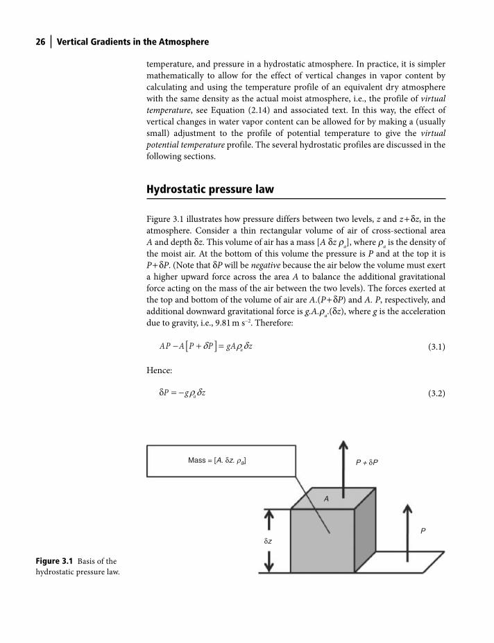
26 Vertical Gradients in the Atmosphere
temperature, and pressure in a hydrostatic atmosphere. In practice, it is simpler
mathematically to allow for the effect of vertical changes in vapor content by
calculating and using the temperature profile of an equivalent dry atmosphere
with the same density as the actual moist atmosphere, i.e., the profile of virtual
temperature, see Equation (2.14) and associated text. In this way, the effect of
vertical changes in water vapor content can be allowed for by making a (usually
small) adjustment to the profile of potential temperature to give the virtual
potential temperature profile. The several hydrostatic profiles are discussed in the
following sections.
Hydrostatic pressure law
Figure 3.1 illustrates how pressure differs between two levels, z and z + δz, in the
atmosphere. Consider a thin rectangular volume of air of cross-sectional area
A and depth δz. This volume of air has a mass [A δz ra], where r
a is the density of
the moist air. At the bottom of this volume the pressure is P and at the top it is
P + δP. (Note that δP will be negative because the air below the volume must exert
a higher upward force across the area A to balance the additional gravitational
force acting on the mass of the air between the two levels). The forces exerted at
the top and bottom of the volume of air are A.(P + δP) and A. P, respectively, and
additional downward gravitational force is g.A.ra.(δz), where g is the acceleration
due to gravity, i.e., 9.81 m s−2. Therefore:
[ ] aAP A P P gA z− + =δ ρ δ
(3.1)
Hence:
aP g zδ = − ρ δ
(3.2)
Mass = [A. δz. ra] P + δP
P
A
δz
Figure 3.1 Basis of the
hydrostatic pressure law.
Shuttleworth_c03.indd 26Shuttleworth_c03.indd 26 11/3/2011 6:31:31 PM11/3/2011 6:31:31 PM
Vertical Gradients in the Atmosphere 27
In the limit of small δz this means:
a
Pg
z
∂= −
∂ρ
(3.3)
Adiabatic lapse rates
The word adiabatic is used to describe changes in which there is no net change in
energy. Here it is used to indicate that we are defining how the temperature of a
parcel of air of volume V would change if it were moved vertically in the atmos-
phere in such a way that there was no net change in the internal energy of the
parcel. The vertical movement of a buoyant air parcel might, for example, be
approximately adiabatic if its ascent is rapid and there is no time for the parcel to
exchange energy with the surrounding air.
The first law of thermodynamics states that the heat added to a system is the
sum of the change in internal energy plus the work done by the system on its sur-
roundings. When applied to the case of an air parcel of volume V moving a small
distance δz in the vertical and undergoing associated small changes δP in pressure
and δT in temperature, this law implies:
p
m
aV H* V c T V Pδ = −ρ d d
(3.4)
where δH* is the heat added per unit volume of air and cp
m is the specific heat at
constant pressure of moist air. The specific heat of moist air varies slightly, but
because the amount of water vapor in moist air is typically just a few percent, it is
generally considered acceptable to use cp = 1.013 kJ kg−1K−1, i.e., the specific heat at
constant pressure for dry air in Equation (3.4) instead of cp
m.
Dry adiabatic lapse rate
When vertical movement of the moist air is adiabatic and the air remains
unsaturated, (δH*) = 0. Equation (3.4) can then be rewritten as:
a pP c T=δ r d
(3.5)
Combining this last equation with Equation (3.2) gives:
δ δ= −p
gT z
c
(3.6)
To a good approximation, both g and cp are constants in the lower atmosphere.
Consequently, for vertical movements of an unsaturated air parcel that occur adiabati-
cally in the atmosphere, the resulting rate of temperature change is constant, i.e.:
Shuttleworth_c03.indd 27Shuttleworth_c03.indd 27 11/3/2011 6:31:35 PM11/3/2011 6:31:35 PM
28 Vertical Gradients in the Atmosphere
T
z
∂= −Γ
∂ (3.7)
where Γ = g/cp is the dry adiabatic lapse rate which is conventionally defined to be
positive, and which has the value 0.00968 K m−1 or 9.68 K km−1.
Moist adiabatic lapse rate
When vertical movement of moist air is adiabatic but the air is saturated,
condensation can occur in the air parcel as it ascends. If its specific humidity
decreases by an amount δqsat
, latent heat is released and the internal energy of the
parcel changes by an amount δH* = (l .ra.δq
sat). Equation (3.4) therefore becomes:
aa sat pV q V c T V P= −λρ δ ρ δ δ
(3.8)
Combining this last equation with Equation (3.2), rearranging in the limit gives an
equation similar to Equation (3.7), i.e.:
m
T
z
∂= −Γ
∂ (3.9)
where Γm
is the moist adiabatic lapse rate given by:
sat
m
p
q
c z
⎛ ⎞∂Γ = Γ −⎜ ⎟∂⎝ ⎠
λ
(3.10)
Because the temperature of the atmosphere normally decreases with height the
saturated specific humidity also decreases with height, hence the rate at which the
temperature falls in a parcel of air ascending in a saturated atmosphere is less than
in an unsaturated atmosphere, i.e., Γm
< Γ. Because qsat
depends on temperature,
the moist adiabatic lapse rate also depends on temperature. For a specific value of
saturated vapor pressure, because the value of qsat
depends on pressure, see
Equation (2.9), Γm
also depends on atmospheric pressure.
Environmental lapse rate
The actual measured rate at which atmospheric temperature changes away from the
ground on a particular day at a particular place depends on the history of heat inputs
and outputs to the air overhead. The locally observed atmospheric lapse rate, which
is called the environmental lapse rate, Γe, therefore varies with location and time.
Near the surface the lapse rate may well be approximately constant, often with
a value intermediate to the dry and moist adiabatic lapse rates. The temperature
Shuttleworth_c03.indd 28Shuttleworth_c03.indd 28 11/3/2011 6:31:39 PM11/3/2011 6:31:39 PM
Vertical Gradients in the Atmosphere 29
profile in the lower troposphere for the US Standard Atmosphere shown in Fig. 1.2
illustrates that this is the case on average, the average near-surface environmental
lapse rate in this case being 6.5 K km−1. However, it is important to emphasize that
the behavior shown in Fig. 1.2 is a temporal and spatial average for all of the USA
and the actual environmental lapse rate on any particular day and at any particu-
lar place will differ from this average profile. The actual environmental lapse rate
and, especially, its relationship to the dry adiabatic lapse rate and the moist
adiabatic lapse rate can affect cloud and precipitation formation, as discussed
in Chapter 10.
Vertical pressure and temperature gradients
Recall that the vertical gradients of atmospheric pressure and temperature are
necessarily linked via the ideal gas law. If Ra is the specific gas constant for moist
air, then by combining Equation (2.5) with Equation (3.2) and rearranging, it can
be shown that the small change in pressure over a vertical distance δz is given by:
a
gPz
P R T= −
δ δ
(3.11)
If Γlocal
is the local environmental lapse rate, then δT = Γlocal
δz. Using this relation-
ship to substitute for δz in Equation (3.11), it follows that the small changes in
pressure and temperature with height are related by:
a local
gP T
P R T
⎛ ⎞= ⎜ ⎟Γ⎝ ⎠
δ δ
(3.12)
If Γlocal
is constant through a portion of the atmosphere then by taking the limit
of Equation (3.12) and integrating between two levels where the air temperatures
(in degrees K) are T1 and T
2, and air pressures P
1 and P
2, it can be easily shown that
across this region:
2
2 1
1
a local
g
RTP P
T
Γ⎛ ⎞= ⎜ ⎟⎝ ⎠
(3.13)
2
2 1
1
a localR
gPT T
P
Γ
⎛ ⎞= ⎜ ⎟⎝ ⎠
(3.14)
Figure 3.2 illustrates the lapse rate and the way atmospheric pressure and air
density consequently change through the lower troposphere for the US Standard
Atmosphere for which Γlocal
= 6.5 K km−1.
Shuttleworth_c03.indd 29Shuttleworth_c03.indd 29 11/3/2011 6:31:42 PM11/3/2011 6:31:42 PM

30 Vertical Gradients in the Atmosphere
Potential temperature
For an adiabatic atmosphere, Γlocal
= g/cp and Equation (3.14) can therefore be
re-written as:
2
2 1
1
a
p
R
cPT T
P
⎛ ⎞= ⎜ ⎟⎝ ⎠
(3.15)
This equation can be used to correct temperature variations in the atmosphere for
the effect of the hydrostatic pressure gradient. If such corrections are made, any
remnant variations in this corrected temperature profile are those which may result
in vertical heat flow as discussed earlier. It is convenient to use Equation (3.15)
to renormalize the observed temperature profile to correspond to a specific value
of pressure, i.e., 100 kPa. When corrected in this way the resulting temperature is
called the potential temperature, q. Potential temperature is therefore defined to be
the temperature that a parcel of air anywhere in the atmosphere would have if it
were to be brought adiabatically to a pressure of 100 kPa. It is calculated from the
actual temperature and pressure using the equation:
100a
p
R
c
TP
⎛ ⎞= ⎜ ⎟⎝ ⎠θ
(3.16)
For a parcel of air moving up or down in an adiabatic atmosphere the value of the
potential temperature is conserved and remains constant with height. To a good
approximation, the vertical gradient of the potential temperature can be calculated
from that for temperature using:
d
T
z z
∂ ∂= + Γ
∂ ∂θ
(3.17)
150 250 0 50 100 0.00
2
4
Hei
ght (
km)
6
8
10
0
2
4
Hei
ght (
km)
6
8
10
0
2
4
Hei
ght (
km)
6
8
10
0.5
Air density (kg m−3)Pressure (kPa)Temperature ( �K)
1.0 1.5
Figure 3.2 Temperature
lapse rate, and pressure and
density variations through
the troposphere of the US
Standard Atmosphere.
Shuttleworth_c03.indd 30Shuttleworth_c03.indd 30 11/3/2011 6:31:46 PM11/3/2011 6:31:46 PM
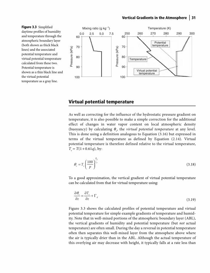
Vertical Gradients in the Atmosphere 31
Virtual potential temperature
As well as correcting for the influence of the hydrostatic pressure gradient on
temperature, it is also possible to make a simple correction for the additional
effect of changes in water vapor content on local atmospheric density
(buoyancy) by calculating qv, the virtual potential temperature at any level.
This is done using a definition analogous to Equation (3.16) but expressed in
terms of the virtual temperature as defined by Equation (2.14). Virtual
potential temperature is therefore defined relative to the virtual temperature,
Tv = T(1 + 0.61q), by:
100a
p
R
c
v vT
P
⎛ ⎞= ⎜ ⎟⎝ ⎠θ
(3.18)
To a good approximation, the vertical gradient of virtual potential temperature
can be calculated from that for virtual temperature using:
v v
d
T
z z
∂ ∂= + Γ
∂ ∂θ
(3.19)
Figure 3.3 shows the calculated profiles of potential temperature and virtual
potential temperature for simple example gradients of temperature and humid-
ity. Note that in well-mixed portions of the atmospheric boundary layer (ABL),
the vertical gradients of humidity and potential temperature (but not actual
temperature) are often small. During the day a reversal in potential temperature
often then separates this well-mixed layer from the atmosphere above where
the air is typically drier than in the ABL. Although the actual temperature of
this overlying air may decrease with height, it typically falls at a rate less than
100
0.0 2.5 5.0
Mixing ratio (g kg−1)
7.5
Pre
ssur
e (k
Pa)
90
80
70
60
100
250 260 270
Temperature (K)
290280
Potentialtemperature
Temperature
Virtual potentialtemperature
300
Pre
ssur
e (k
Pa)
90
80
70
60
Figure 3.3 Simplified
daytime profiles of humidity
and temperature through the
atmospheric boundary layer
(both shown as thick black
lines) and the associated
potential temperature and
virtual potential temperature
calculated from these two.
Potential temperature is
shown as a thin black line and
the virtual potential
temperature as a gray line.
Shuttleworth_c03.indd 31Shuttleworth_c03.indd 31 11/3/2011 6:31:49 PM11/3/2011 6:31:49 PM
32 Vertical Gradients in the Atmosphere
the dry adiabatic lapse rate, so the potential temperature of the overlying air is
greater than the air in the ABL. In general (and in Fig. 3.3), virtual potential
temperature is typically just a few degrees greater than potential temperature,
the difference being directly related to the specific humidity of the atmosphere,
see Equation (2.8).
Atmospheric stability
If a parcel of air moves up or down in the atmosphere (perhaps in response to
atmospheric turbulence) it is likely that it will find itself in a new environment
whose temperature and density differs from that which would have resulted from
adiabatic warming or cooling of the parcel. Any resulting density difference
between the parcel and the air that surrounds it will give rise to a buoyancy force
which will influence further vertical movement of the parcel.
If after moving, the parcel has a higher temperature and is less dense and lighter
than the air it displaces, it is said to be unstable in its new location and further
upward movement will be encouraged and downward movement inhibited. If
after moving the parcel has a lower temperature and is more dense and heavier
than the air it displaces, it is said to be stable in its new location and further upward
movement will be inhibited and downward movement encouraged. If after
moving, the parcel has the same temperature and density as the air it displaces, it
is said to be neutral with respect to the environment in its new location and further
movement is neither encouraged nor inhibited.
Static stability parameter
From Archimedes principle, if a parcel of air with density ra′ moves vertically and
displaces the same volume of surrounding air with density ra, it will be subject to
a force such as to cause a buoyant acceleration, ap, given by:
( )a a
p
a
a g′ −
= −ρ ρ
ρ
(3.20)
Assuming the pressure of both parcels is the same, substituting for densities using
Equation (2.11) this last equation becomes:
( )v v
p
T Ta g
T
− ′= −
(3.21)
where Tv’ and T
v are the virtual temperatures of the parcel and the surrounding air,
respectively. If vertical air movement is viewed in terms of small displacements,
Shuttleworth_c03.indd 32Shuttleworth_c03.indd 32 11/3/2011 6:31:51 PM11/3/2011 6:31:51 PM
Vertical Gradients in the Atmosphere 33
δz, along the vertical gradients of virtual temperature, Tv, or virtual potential
temperature, qv, buoyant acceleration can be written as:
v
p d
v
Tga z
T z
⎛ ⎞ ∂⎛ ⎞= − + Γ⎜ ⎟⎜ ⎟ ⎝ ⎠∂⎝ ⎠
δ
(3.22)
or:
v
p
v
ga z
z
⎛ ⎞ ∂= −⎜ ⎟ ∂⎝ ⎠
θδ
θ
(3.23)
The static stability parameter, s, is defined from buoyant acceleration using this last
equation and has the form:
v
v
gs
z
⎛ ⎞ ∂= −⎜ ⎟ ∂⎝ ⎠
θθ
(3.24)
The parameter s provides a quantitative measure of the static stability of atmos-
phere at any level in terms of the potential temperature gradient at that level. Thus,
the atmosphere is said to be:
(a) Unstable: when s < 0, i.e., when (∂qv�∂z) < 0 or (∂T
v�∂z) < −Γ
d
That is, when virtual temperature falls more quickly than the dry
adiabatic lapse rate – in which condition the atmosphere is said to be
superadiabatic.
(b) Neutral: when s = 0, i.e., when (∂qv�∂z) = 0 or (∂T
v�∂z) = −Γ
d
That is, when virtual temperature falls at the dry adiabatic lapse – in which
condition the atmosphere is said to be adiabatic.
(c) Stable: when s > 0, i.e., when (∂qv�∂z) > 0 or (∂T
v�∂z) > −Γ
d
That is, when virtual temperature falls less quickly than the dry
adiabatic lapse rate – in which condition the atmosphere is said to be
subadiabatic.
In addition, certain subadiabatic (stable) atmospheric conditions are further
distinguished by their gradients of virtual temperature, as follows:
(1) if Tv is constant with height, the atmosphere is said to be isothermal;
(2) if Tv increases with height, there is said to be an inversion,
Figure 3.4 illustrates how the vertical gradient of virtual temperature is used
to characterize atmospheric conditions. In Chapter 20 an alternative measure
of atmospheric stability is defined based on the turbulent fluxes through
the atmosphere.
Shuttleworth_c03.indd 33Shuttleworth_c03.indd 33 11/3/2011 6:31:53 PM11/3/2011 6:31:53 PM
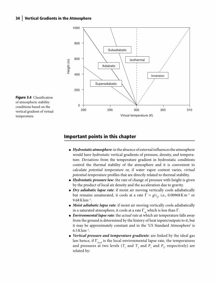
34 Vertical Gradients in the Atmosphere
Important points in this chapter
● Hydrostatic atmosphere: in the absence of external influences the atmosphere
would have hydrostatic vertical gradients of pressure, density, and tempera-
ture. Deviations from the temperature gradient in hydrostatic conditions
control the thermal stability of the atmosphere and it is convenient to
calculate potential temperature or, if water vapor content varies, virtual
potential temperature profiles that are directly related to thermal stability.
● Hydrostatic pressure law: the rate of change of pressure with height is given
by the product of local air density and the acceleration due to gravity.
● Dry adiabatic lapse rate: if moist air moving vertically cools adiabatically
but remains unsaturated, it cools at a rate Γ = g/cp, i.e., 0.00968 K m−1 or
9.68 K km−1.
● Moist adiabatic lapse rate: if moist air moving vertically cools adiabatically
in a saturated atmosphere, it cools at a rate Γm
which is less than Γ.
● Environmental lapse rate: the actual rate at which air temperature falls away
from the ground is determined by the history of heat inputs/outputs to it, but
it may be approximately constant and in the ‘US Standard Atmosphere’ is
6.5 K km−1.
● Vertical pressure and temperature gradients: are linked by the ideal gas
law hence, if Γlocal
is the local environmental lapse rate, the temperatures
and pressures at two levels (T1 and T
2 and P
1 and P
2, respectively) are
related by:
0290 295 300 305 310
Virtual temperature (K)
Subadiabatic
Superadiabatic
Inversion
Isothermal
Adiabatic
200
400Hei
ght (
m) 600
800
1000
Figure 3.4 Classification
of atmospheric stability
conditions based on the
vertical gradient of virtual
temperature.
Shuttleworth_c03.indd 34Shuttleworth_c03.indd 34 11/3/2011 6:31:56 PM11/3/2011 6:31:56 PM
Vertical Gradients in the Atmosphere 35
( ) ( )( )2 1 2 1
a localR g
T T P PΓ
=
(3.25)
● Potential temperature: the temperature that a parcel of air in the atmosphere
would have if it were to be brought adiabatically to a pressure of 100 kPa, q, is:
( )( )100
a pR c
T P=θ
(3.26)
The gradient of potential temperature is that for actual temperature minus Γ.
● Virtual potential temperature: analogous to potential temperature, qv is:
( )( )(1 0.61 ) 100
a pR c
vT q P= +θ
(3.27)
The gradient of virtual potential temperature is that for virtual temperature
minus Γ.
● Atmospheric stability: the gradient of qv determines atmospheric stability,
thus:
Unstable: (∂qv/∂z) < 0 Neutral: (∂q
v/∂z) = 0 Stable: (∂q
v/∂z) > 0 (3.28)
Some stable conditions are further distinguished:
Isothermal: Tv is constant with height: Inversion: T
v increases
with height (3.29)
Shuttleworth_c03.indd 35Shuttleworth_c03.indd 35 11/3/2011 6:31:56 PM11/3/2011 6:31:56 PM
Introduction
Terrestrial surfaces influence and are influenced by the overlying atmosphere
through the exchange of energy, water, and other atmospheric constituents. In this
chapter we consider the exchange of energy that occurs mainly in the form of sur-
face fluxes of radiant energy, latent heat (when water vapor evaporates from or
condenses onto the land), sensible heat (that warms or cools the air in contact with
the surface), and heat that diffuses into or out of the ground.
The surface flux of any entity is the amount of that entity flowing through and
normal to the surface in unit time, per unit surface area. In the case of energy flux
exchange with terrestrial surfaces, this is the rate of flow of energy per unit area
of land surface. In Système International (SI) units, surface energy fluxes are
expressed in units of Joules per second per square meter, but one Joule per second
is one Watt, consequently the units of surface energy fluxes are Watts per square
meter (W m−2). For terrestrial surfaces, the maximum rates of surface energy
transfer are constrained by the incoming energy from the Sun. At the top of the
atmosphere, the time average energy flux arriving from the Sun when directly
overhead is ∼1366 W m−2: this value is called the Solar Constant. Typically 25–75%
of the Sun’s energy is absorbed as it travels through the atmosphere depending
mainly on cloud cover, so the incoming energy arriving at the surface as solar
radiation could be ∼1000 W m−2 in clear sky conditions at midday near the
equator. However, it is typically much less than this at other times of day and at
higher latitudes, and there is no incoming solar radiation during the night.
The energy incoming as solar radiation is shared between several surface fluxes,
consequently the order of magnitude of such energy fluxes is typically a few 10s
to a few 100s of W m−2.
4 Surface Energy Fluxes
Terrestrial Hydrometeorology, First Edition. W. James Shuttleworth.
© 2012 John Wiley & Sons, Ltd. Published 2012 by John Wiley & Sons, Ltd.
Shuttleworth_c04.indd 36Shuttleworth_c04.indd 36 11/3/2011 6:34:00 PM11/3/2011 6:34:00 PM

Surface Energy Fluxes 37
Terrestrial surfaces often have heterogeneous land cover and the nature of this
cover can substantially alter the amount of solar radiation captured at the surface
and the way in which this is then shared as surface energy fluxes. In hydrometeorology
and hydroclimatology, heterogeneous terrestrial surfaces are often imagined as
being made up of a patchwork of ideal surfaces, with each ideal patch assumed to be
opaque to radiation and acceptably homogeneous in terms of those surface
characteristics that influence surface energy fluxes. It is further assumed that above
a certain level in the atmospheric boundary layer (say 50–100 m) the atmosphere is
well-mixed so atmospheric variables can be considered independent of the
underlying patch. This height is called the blending height. The land surface
characteristics that influence surface energy exchange and are assumed to be
homogeneous across an ideal patch include the vegetation-dependent reflection
coefficient for solar radiation, thermal emissivity, aerodynamic roughness, and
the ability to capture and store precipitation on plant canopies or in the soil accessible
by plant roots. Often in atmospheric models ideal patches are also assumed to be
horizontal, and even if not horizontal, it is at least assumed that the flow of energy
into or out of the atmosphere is vertical.
Latent and sensible heat fluxes
In SI units the evaporation flux, E, has the units of kilograms of evaporated water
per second per square meter of land surface. Conveniently, because the density of
water is close to 1 kg l−1, 1 kg s−1 m−2 of evaporated water is equivalent to 1 mm s−1
depth of water evaporated. However, surface evaporation rates of the order 1 mm s−1
do not occur in the natural world: evaporation rates are more typically on the
order of a few mm day−1 because the latent heat needed to support evaporation is
constrained by the Earth’s surface energy balance.
It is very common to quantify evaporation rates from terrestrial surfaces not in
terms of mass flow but in terms of the flow of energy leaving the evaporating surface
as latent heat of vaporization in the water vapor. To express the rate of evaporation
as the latent heat flux, λE, in W m−2, the evaporation flux E, in kg s−1 m−2, is multiplied
by λ, the latent heat of vaporization of water in J kg−1. Hydrologists more used to
working in terms of the mass balance of water rather than the surface energy
balance find it useful to remember that an evaporation rate of 3.5 mm d−1 is
equivalent to a daily average latent heat flux of 100 W m−2, and an evaporation rate
of 1 mm d−1 is equivalent to a daily average latent heat flux of 28.6 W m−2 (i.e., about
30 W m−2).
The flow of energy as latent heat away from or toward the land surface is very
important, but it is not the only way the energy can be exchanged with the
atmosphere. A second important way is by the surface directly warming or cool-
ing the air in contact with the surface, with heat then either diffusing outward to
the air above or inward from the air above, respectively. The associated flow of
energy is called the sensible heat flux because it is associated with changes in air
Shuttleworth_c04.indd 37Shuttleworth_c04.indd 37 11/3/2011 6:34:01 PM11/3/2011 6:34:01 PM
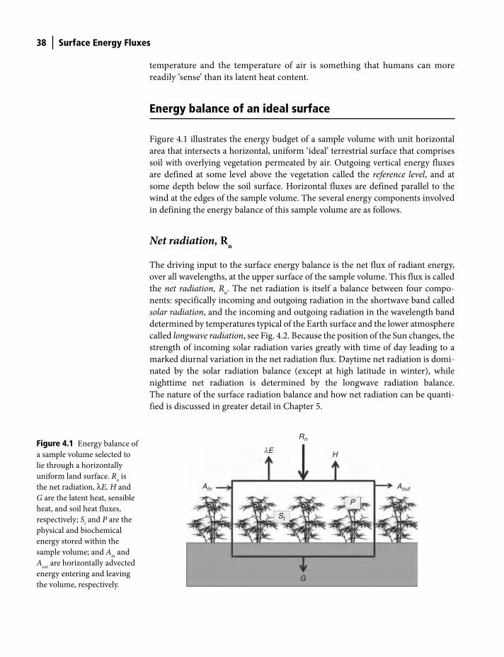
38 Surface Energy Fluxes
temperature and the temperature of air is something that humans can more
readily ‘sense’ than its latent heat content.
Energy balance of an ideal surface
Figure 4.1 illustrates the energy budget of a sample volume with unit horizontal
area that intersects a horizontal, uniform ‘ideal’ terrestrial surface that comprises
soil with overlying vegetation permeated by air. Outgoing vertical energy fluxes
are defined at some level above the vegetation called the reference level, and at
some depth below the soil surface. Horizontal fluxes are defined parallel to the
wind at the edges of the sample volume. The several energy components involved
in defining the energy balance of this sample volume are as follows.
Net radiation, Rn
The driving input to the surface energy balance is the net flux of radiant energy,
over all wavelengths, at the upper surface of the sample volume. This flux is called
the net radiation, Rn. The net radiation is itself a balance between four compo-
nents: specifically incoming and outgoing radiation in the shortwave band called
solar radiation, and the incoming and outgoing radiation in the wavelength band
determined by temperatures typical of the Earth surface and the lower atmosphere
called longwave radiation, see Fig. 4.2. Because the position of the Sun changes, the
strength of incoming solar radiation varies greatly with time of day leading to a
marked diurnal variation in the net radiation flux. Daytime net radiation is domi-
nated by the solar radiation balance (except at high latitude in winter), while
nighttime net radiation is determined by the longwave radiation balance.
The nature of the surface radiation balance and how net radiation can be quanti-
fied is discussed in greater detail in Chapter 5.
Figure 4.1 Energy balance of
a sample volume selected to
lie through a horizontally
uniform land surface. Rn is
the net radiation, λE, H and
G are the latent heat, sensible
heat, and soil heat fluxes,
respectively; St and P are the
physical and biochemical
energy stored within the
sample volume; and Ain
and
Aout
are horizontally advected
energy entering and leaving
the volume, respectively.G
lE
Rn
H
AoutAin
St
P
Shuttleworth_c04.indd 38Shuttleworth_c04.indd 38 11/3/2011 6:34:01 PM11/3/2011 6:34:01 PM
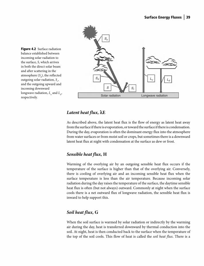
Surface Energy Fluxes 39
Latent heat flux, lE
As described above, the latent heat flux is the flow of energy as latent heat away
from the surface if there is evaporation, or toward the surface if there is condensation.
During the day, evaporation is often the dominant energy flux into the atmosphere
from water surfaces or from moist soil or crops, but sometimes there is a downward
latent heat flux at night with condensation at the surface as dew or frost.
Sensible heat flux, H
Warming of the overlying air by an outgoing sensible heat flux occurs if the
temperature of the surface is higher than that of the overlying air. Conversely,
there is cooling of overlying air and an incoming sensible heat flux when the
surface temperature is less than the air temperature. Because incoming solar
radiation during the day raises the temperature of the surface, the daytime sensible
heat flux is often (but not always) outward. Commonly at night when the surface
cools there is a net outward flux of longwave radiation, the sensible heat flux is
inward to help support this.
Soil heat flux, G
When the soil surface is warmed by solar radiation or indirectly by the warming
air during the day, heat is transferred downward by thermal conduction into the
soil. At night, heat is then conducted back to the surface when the temperature of
the top of the soil cools. This flow of heat is called the soil heat flux. There is a
Figure 4.2 Surface radiation
balance established between
incoming solar radiation to
the surface, S, which arrives
in both the direct solar beam
and after scattering in the
atmosphere (Sd), the reflected
outgoing solar radiation, Sr ,
and the outgoing upward and
incoming downward
longwave radiation, Lu and L
d ,
respectively.Solar radiation Longwave radiation
SrS
Sd
So
Lu Ld
Shuttleworth_c04.indd 39Shuttleworth_c04.indd 39 11/3/2011 6:34:02 PM11/3/2011 6:34:02 PM
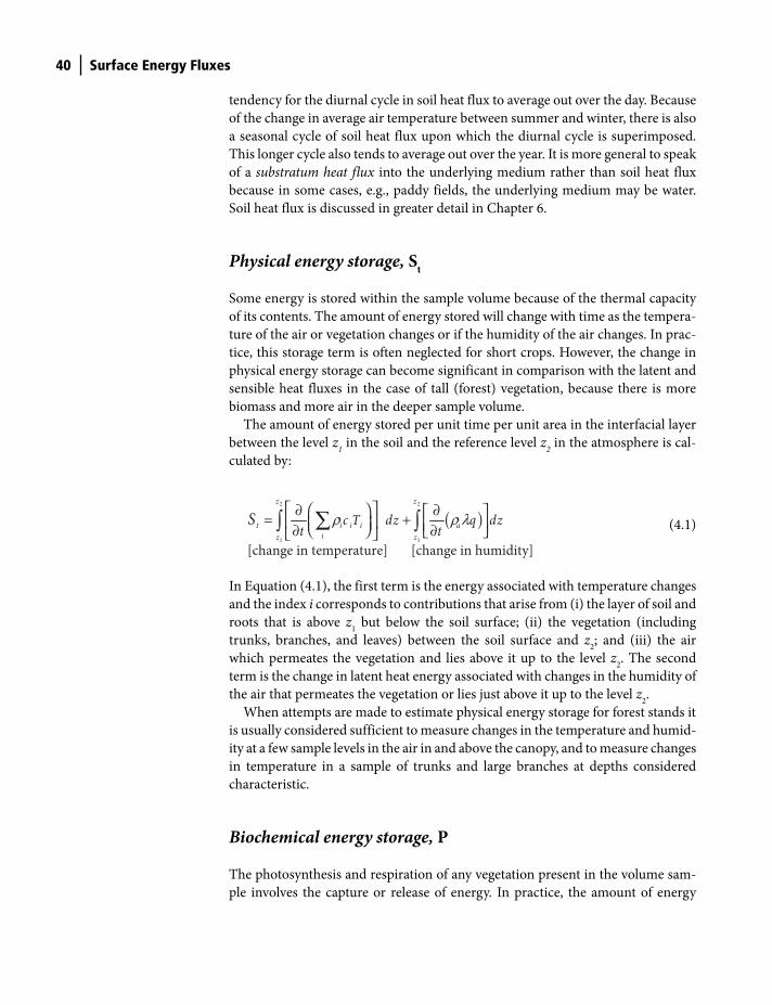
40 Surface Energy Fluxes
tendency for the diurnal cycle in soil heat flux to average out over the day. Because
of the change in average air temperature between summer and winter, there is also
a seasonal cycle of soil heat flux upon which the diurnal cycle is superimposed.
This longer cycle also tends to average out over the year. It is more general to speak
of a substratum heat flux into the underlying medium rather than soil heat flux
because in some cases, e.g., paddy fields, the underlying medium may be water.
Soil heat flux is discussed in greater detail in Chapter 6.
Physical energy storage, St
Some energy is stored within the sample volume because of the thermal capacity
of its contents. The amount of energy stored will change with time as the tempera-
ture of the air or vegetation changes or if the humidity of the air changes. In prac-
tice, this storage term is often neglected for short crops. However, the change in
physical energy storage can become significant in comparison with the latent and
sensible heat fluxes in the case of tall (forest) vegetation, because there is more
biomass and more air in the deeper sample volume.
The amount of energy stored per unit time per unit area in the interfacial layer
between the level z1 in the soil and the reference level z
2 in the atmosphere is cal-
culated by:
( )ρ ρ λ⎡ ⎤∂ ⎛ ⎞ ∂⎡ ⎤= +⎢ ⎥⎜ ⎟ ⎢ ⎥⎝ ⎠∂ ∂⎣ ⎦⎣ ⎦
∑∫ ∫2 2
1 1
[change in temperature] [change in humidity]
z z
t i i i aiz z
c T dz q dzt t
S (4.1)
In Equation (4.1), the first term is the energy associated with temperature changes
and the index i corresponds to contributions that arise from (i) the layer of soil and
roots that is above z1 but below the soil surface; (ii) the vegetation (including
trunks, branches, and leaves) between the soil surface and z2; and (iii) the air
which permeates the vegetation and lies above it up to the level z2. The second
term is the change in latent heat energy associated with changes in the humidity of
the air that permeates the vegetation or lies just above it up to the level z2.
When attempts are made to estimate physical energy storage for forest stands it
is usually considered sufficient to measure changes in the temperature and humid-
ity at a few sample levels in the air in and above the canopy, and to measure changes
in temperature in a sample of trunks and large branches at depths considered
characteristic.
Biochemical energy storage, P
The photosynthesis and respiration of any vegetation present in the volume sam-
ple involves the capture or release of energy. In practice, the amount of energy
Shuttleworth_c04.indd 40Shuttleworth_c04.indd 40 11/3/2011 6:34:02 PM11/3/2011 6:34:02 PM
Surface Energy Fluxes 41
involved in plant photochemistry is usually comparatively small (on the order of
2% of the incoming solar energy). For this reason this energy term is often
neglected in hydrometeorology.
Advected energy, Ad
The net advected energy, Ad = A
in – A
out (see Fig. 4.2), is also usually neglected for
homogeneous ideal surfaces, but can become significant in ‘oasis’ situations.
Flux sign convention
The sign convention most often used for the several terms in the energy budget
summarized above is biased toward the value of fluxes being positive in daytime
conditions. Consequently:
(a) all radiation fluxes are defined as being positive when directed toward the
surface (this applies to Rn and its component fluxes S, S
d, S
r, L
u and L
d, see
Fig. 4.2).
(b) all the other vertical energy fluxes are defined as being positive when
directed away from the surface (this applies to λE, H, and G)
(c) the storage terms are defined as being positive when they take in energy
(this applies to St and P)O
(d) if considered, the net advected energy, Ad, is defined as positive when it
brings energy into the sample volume.
Consistent with this sign convention, the overall energy budget for the sample
volume through an ideal surface shown in Fig. 4.1 is written as:
( ) ( )n t tR G A S P E H− + − − = +l (4.2)
The terms on the left of Equation 4.2 are usually grouped together in this way
because in daytime conditions they together define the energy available in the
energy budget that is shared between the latent and sensible heat on the right. For
this reason this set of terms is sometimes referred to as the available energy, A,
which is defined by:
( )n t tA R G A S P= − + − − (4.3)
The magnitudes and, in the case of vertical energy fluxes, the direction of terms
in the surface energy budget are characteristically different in daytime and
nighttime conditions, and they also depend strongly on whether the surface is
bare soil or covered with vegetation and also on how much moisture is available
in the soil.
Shuttleworth_c04.indd 41Shuttleworth_c04.indd 41 11/3/2011 6:34:03 PM11/3/2011 6:34:03 PM
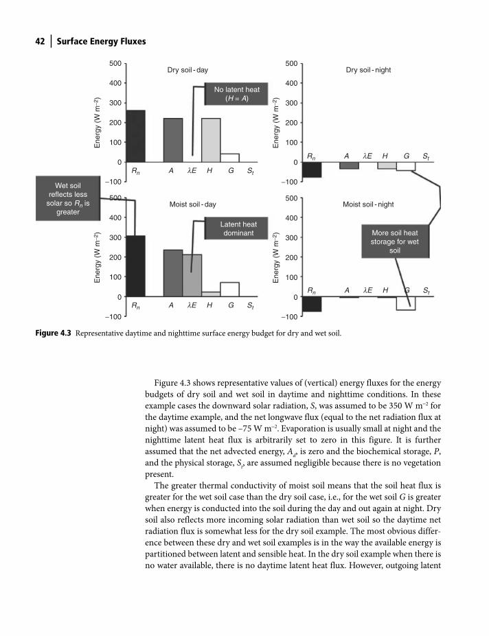
42 Surface Energy Fluxes
Figure 4.3 shows representative values of (vertical) energy fluxes for the energy
budgets of dry soil and wet soil in daytime and nighttime conditions. In these
example cases the downward solar radiation, S, was assumed to be 350 W m−2 for
the daytime example, and the net longwave flux (equal to the net radiation flux at
night) was assumed to be –75 W m−2. Evaporation is usually small at night and the
nighttime latent heat flux is arbitrarily set to zero in this figure. It is further
assumed that the net advected energy, Ad, is zero and the biochemical storage, P,
and the physical storage, St, are assumed negligible because there is no vegetation
present.
The greater thermal conductivity of moist soil means that the soil heat flux is
greater for the wet soil case than the dry soil case, i.e., for the wet soil G is greater
when energy is conducted into the soil during the day and out again at night. Dry
soil also reflects more incoming solar radiation than wet soil so the daytime net
radiation flux is somewhat less for the dry soil example. The most obvious differ-
ence between these dry and wet soil examples is in the way the available energy is
partitioned between latent and sensible heat. In the dry soil example when there is
no water available, there is no daytime latent heat flux. However, outgoing latent
Wet soilreflects less
solar so Rn isgreater
Rn A lE H G St
Moist soil - day Moist soil - night
No latent heat(H = A)
Latent heatdominant More soil heat
storage for wetsoil
−100
100
200
300
400
500
0
Rn A lE H G St
−100
100
200
300
400
500
0
Dry soil - day
Ene
rgy
(W m
−2)
Ene
rgy
(W m
−2)
Rn A lE H G St
−100
100
200
300
400
500
0
Dry soil - night
Ene
rgy
(W m
−2)
Rn A lE H G St
−100
100
200
300
400
500
0
Ene
rgy
(W m
−2)
Figure 4.3 Representative daytime and nighttime surface energy budget for dry and wet soil.
Shuttleworth_c04.indd 42Shuttleworth_c04.indd 42 11/3/2011 6:34:05 PM11/3/2011 6:34:05 PM
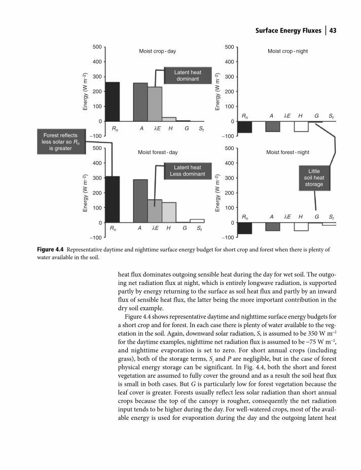
Surface Energy Fluxes 43
heat flux dominates outgoing sensible heat during the day for wet soil. The outgo-
ing net radiation flux at night, which is entirely longwave radiation, is supported
partly by energy returning to the surface as soil heat flux and partly by an inward
flux of sensible heat flux, the latter being the more important contribution in the
dry soil example.
Figure 4.4 shows representative daytime and nighttime surface energy budgets for
a short crop and for forest. In each case there is plenty of water available to the veg-
etation in the soil. Again, downward solar radiation, S, is assumed to be 350 W m−2
for the daytime examples, nighttime net radiation flux is assumed to be −75 W m−2,
and nighttime evaporation is set to zero. For short annual crops (including
grass), both of the storage terms, St and P are negligible, but in the case of forest
physical energy storage can be significant. In Fig. 4.4, both the short and forest
vegetation are assumed to fully cover the ground and as a result the soil heat flux
is small in both cases. But G is particularly low for forest vegetation because the
leaf cover is greater. Forests usually reflect less solar radiation than short annual
crops because the top of the canopy is rougher, consequently the net radiation
input tends to be higher during the day. For well-watered crops, most of the avail-
able energy is used for evaporation during the day and the outgoing latent heat
Forest reflectsless solar so Rn
is greater
Rn A lE H G St
Moist forest - day Moist forest - night
Latent heatdominant
Latent heatLess dominant Little
soil heatstorage
−100
100
200
300
400
500
0
Rn A lE H G St
−100
100
200
300
400
500
0
Moist crop - day Moist crop - night
Ene
rgy
(W m
−2)
Ene
rgy
(W m
−2)
Rn A lE H G St
−100
100
200
300
400
500
0
Ene
rgy
(W m
−2)
Rn A lE H G St
−100
100
200
300
400
500
0E
nerg
y (W
m−2
)
Figure 4.4 Representative daytime and nighttime surface energy budget for short crop and forest when there is plenty of
water available in the soil.
Shuttleworth_c04.indd 43Shuttleworth_c04.indd 43 11/3/2011 6:34:05 PM11/3/2011 6:34:05 PM
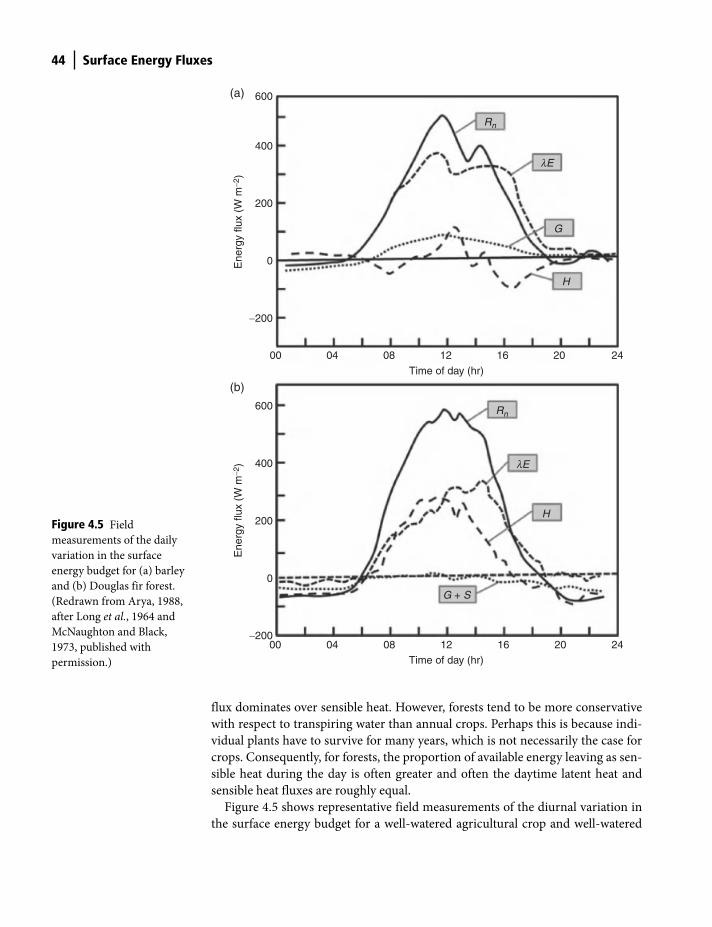
44 Surface Energy Fluxes
flux dominates over sensible heat. However, forests tend to be more conservative
with respect to transpiring water than annual crops. Perhaps this is because indi-
vidual plants have to survive for many years, which is not necessarily the case for
crops. Consequently, for forests, the proportion of available energy leaving as sen-
sible heat during the day is often greater and often the daytime latent heat and
sensible heat fluxes are roughly equal.
Figure 4.5 shows representative field measurements of the diurnal variation in
the surface energy budget for a well-watered agricultural crop and well-watered
−200
00 04
Rn
lE
G
H
08 12
Time of day (hr)
16 20 24
Ene
rgy
flux
(W m
−2)
200
(a)
400
600
0
−20000 04
Rn
lE
G + S
H
08 12Time of day (hr)
16 20 24
200
Ene
rgy
flux
(W m
−2)
(b)
400
600
0
Figure 4.5 Field
measurements of the daily
variation in the surface
energy budget for (a) barley
and (b) Douglas fir forest.
(Redrawn from Arya, 1988,
after Long et al., 1964 and
McNaughton and Black,
1973, published with
permission.)
Shuttleworth_c04.indd 44Shuttleworth_c04.indd 44 11/3/2011 6:34:06 PM11/3/2011 6:34:06 PM

Surface Energy Fluxes 45
forest. For the well-watered crop (a) daytime latent heat flux typically consumes
70–90% of net radiation, as in this example, and the sensible and soil heat fluxes
can be of similar magnitude. Notice that this example data shows evaporation con-
tinuing into the evening with the energy in excess of net radiation primarily being
provided by a downward sensible heat flux. The behavior shown is also broadly
typical for forest vegetation, with the outgoing daytime fluxes of latent and sensi-
ble heat more similar than for the crop. In the figure showing the forest (b), the soil
heat flux and physical energy storage terms are plotted as a sum. In practice the
physical storage term is likely to be the greater of these two.
Evaporative fraction and Bowen ratio
The ratio of the latent heat flux to the sum of the sensible heat flux and latent heat
flux is called the evaporative fraction, EF. If the instantaneous values of sensible and
latent heat are H and λE, respectively, the instantaneous value of the evaporative
fraction is therefore given by:
( )FEE
H E=
+l
l (4.4)
Similarly, if the time average values of sensible and latent heat over a specific time
period are H and Eλ respectively, FE , the evaporative fraction of the average
fluxes over this same period is given by:
( )FEE
H E=
+l
l (4.5)
It is important to recognize that, because the ratio EF may change rapidly with
time, the time-average of instantaneous values of EF does not reliably give the daily
evaporative fraction of the average fluxes, the evaporative fraction for a day must
be calculated from the all-day average fluxes.
The ratio of the sensible heat flux to the latent heat flux is called the Bowen
Ratio, β. If the instantaneous values of sensible and latent heat are H and λE,
respectively, the instantaneous value of the Bowen Ratio is therefore given by:
HE
=bl
(4.6)
Similarly, if the time-average values of sensible and latent heat over a specified
time period are H and Eλ respectively, the time-average Bowen Ratio over this
same period, b , is given by:
HE
=bl
(4.7)
Shuttleworth_c04.indd 45Shuttleworth_c04.indd 45 11/3/2011 6:34:06 PM11/3/2011 6:34:06 PM
46 Surface Energy Fluxes
Again, because β is a rapidly changing ratio, the value of b is not reliably given by
taking the time average of the instantaneous values of β. The average value of β
must be calculated from the two time-average fluxes.
Energy budget of open water
Measuring the energy balance components for expanses of water is difficult partly
because of the practical problems involved in mounting and maintaining relevant
equipment, but also more fundamentally because the fluid to fluid interface
problem is poorly specified. But often it is only the surface heat fluxes (especially
the latent heat flux) exchanges that are needed and attempts have been made to
measure these using micrometeorological methods or, in the case of latent heat,
using a water balance approach to determine the net evaporation.
The evaporation flux from open water is very strongly related to wind speed and
to the difference between the (saturated) vapor pressure at the water surface and
the vapor pressure at some level (usually 2 m) above the surface. Given the
comparative simplicity of the physics describing the exchange in the atmosphere
between the water surface and air, and the difficulty involved in making
measurements, evaporation rates are sometimes estimated from semi-empirical
equations that were derived by calibration against prior careful measurements.
Because near surface air is progressively modified as it moves across a water
surface to an extent that depends on the distance traveled, these semi-empirical
equations are also expressed in terms of the surface area, Aw, of the evaporating
water.
If the measured wind speed at 2 m is U2, and the surface temperature of the
evaporating water is Ts, for small water areas such that 0.5 m < A
w0.5 < 5 m (includ-
ing evaporating pans), an estimate of the evaporation in mm d−1 is:
( )0.066
2 3.623 w sat sE A e T e U− ⎡ ⎤= −⎣ ⎦ (4.8)
where e is the vapor pressure at 2 m and esat
(Ts) is the saturated vapor pressure at
temperature Ts. For larger areas where 50 m < A
w0.5< 100 km, such as lakes, an
estimate of the evaporation in mm d−1 is:
( )0.05
2 2.909 w sat sE A e T e U− ⎡ ⎤= −⎣ ⎦ (4.9)
Important points in this chapter
● Ideal surfaces: in many applications, including hydrological and
meteorological models, the land surface is assumed to be made up of a
patchwork, each patch being homogeneous in terms of surface characteristics
that influence surface energy fluxes.
Shuttleworth_c04.indd 46Shuttleworth_c04.indd 46 11/3/2011 6:34:15 PM11/3/2011 6:34:15 PM
Surface Energy Fluxes 47
● Latent and sensible heat flux: natural evaporation rate (typically a few mm
per day) is converted to latent heat flux by multiplying by the latent heat of
vaporization which has units of W m−2 (1 mm d−1 is equivalent to 28.6 W m−2).
The flow of heat leaving the surface and directly warming the air (in the same
units) is called the sensible heat flux.
● Energy balance: the energy budget of a volume with unit horizontal area that
intersects a horizontal, uniform ideal terrestrial surface that comprises soil
with overlying vegetation permeated by air is (lE + H) = (Rn − G + A
t − S
t − P)
where:
lE is the latent heat flux (see above);
H is the sensible heat flux (see above);
Rn is the net radiation (the net flux of radiant energy at all wavelengths);
G is the soil heat flux (the flow of heat into or out of the soil by conduction);
At is advected energy (the energy advected horizontally in the air by wind);
St is the storage (the change in energy stored in vegetation, air and soil);
P is the biochemical storage (energy stored by photosynthesis/respiration).
● Sign convention: radiation fluxes are positive toward the surface; other verti-
cal energy fluxes are positive away from the surface; storage terms are positive
when energy is absorbed, and advection positive when energy is brought in.
● Difference values of fluxes: examples given are:
— Dry Soil versus Wet Soil: During the day there is no latent heat flux for dry
soil and net radiation is greater for wet soil because less solar energy is
reflected; wet soil has higher thermal conductivity so soil heat fluxes are
greater.
— Moist Crop versus Moist Forest: Forests reflect less solar radiation so day-
time net radiation is higher, but also transpire less so latent heat is less
dominant than for crops; soil heat fluxes are small under dense
vegetation.
● Evaporative fraction and Bowen ratio: evaporative fraction is the ratio of the
latent heat flux to the sum of latent heat plus sensible heat (called the avail-
able energy); Bowen ratio is the ratio of the sensible heat to the latent heat
flux.
● Open water evaporation: is related to wind speed and the difference between
the vapor pressure of the air and the (saturated) vapor pressure at the water
surface by empirical formulae that change with the evaporating area.
References
Arya, S.P. (1988) Introduction to Micrometeorology. Academic Press, San Diego.
Long, I.F., Monteith, J.L., Penman, H.L. and Szeicz, G. (1964) The plant and its environ-
ment. Meteorologische Rundschau, 17, 97–102.
McNaughton K.G. & Black, T.A. (1973) A study of evapotranspiration from a Douglas fir
forest using the energy balance approach. Water Resources Research. 9 (6), 1579–90,
doi:10.1029/WR009i006p01579.
Shuttleworth_c04.indd 47Shuttleworth_c04.indd 47 11/3/2011 6:34:18 PM11/3/2011 6:34:18 PM

Introduction
Surface energy transfer as electromagnetic radiation is a very substantial
component of the Earth−atmosphere system; it is important because it is the driving
force for hydroclimatic movement. In comparison with other energy exchanges that
are slower because they involve transfers via the physical movement of molecules
or portions of air, radiation transfer occurs at the speed of light, c = 3 × 10⁸ m s−1
and is effectively instantaneous. As Fig. 5.1 shows, electromagnetic radiation
covers a wide spectrum of wavelengths. Note that in physics it is conventional to
use the symbol l to describe wavelength and this convention is adopted in this
chapter, although elsewhere in this text the symbol l is used to describe the latent
heat of vaporization of water.
When considering the terrestrial radiation balance at the surface, it is helpful to
remember that anything with a temperature above absolute zero emits radiation
with a spectrum and at a rate that reflects the temperature of the emitting entity.
In the case of terrestrial radiation two radiators are important, the Sun, and the
Earth’s surface and atmosphere. The Sun has a temperature of around 6000 K and
emits shortwave or solar radiation, while the Earth’s surface and lower atmosphere
typically has a temperature of ∼290 K and emits thermal or longwave radiation.
Consequently, at the Earth’s surface the majority of the radiation exchange is via
radiation which lies in the wavelength range 0.1–100 μm (1 μm = 10−6 m). Most
is in the visible (0.39–0.77 μm), near infrared (0.77–25 μm) and far infrared
(25–1000 μm) wavebands, but there is also some in the ultraviolet (0.001–0.39 μm)
waveband. The visible portion of the spectrum is the radiation we see, but we are
aware of infrared radiation because it warms us, and ultraviolet radiation because
it tans our skin.
Figure 5.2 shows that in practice most solar energy is in the wavelength range
0.15–4 μm while most of the energy in terrestrial radiation is in the wavelength
5 Terrestrial Radiation
Terrestrial Hydrometeorology, First Edition. W. James Shuttleworth.
© 2012 John Wiley & Sons, Ltd. Published 2012 by John Wiley & Sons, Ltd.
Shuttleworth_c05.indd 48Shuttleworth_c05.indd 48 11/3/2011 6:32:57 PM11/3/2011 6:32:57 PM
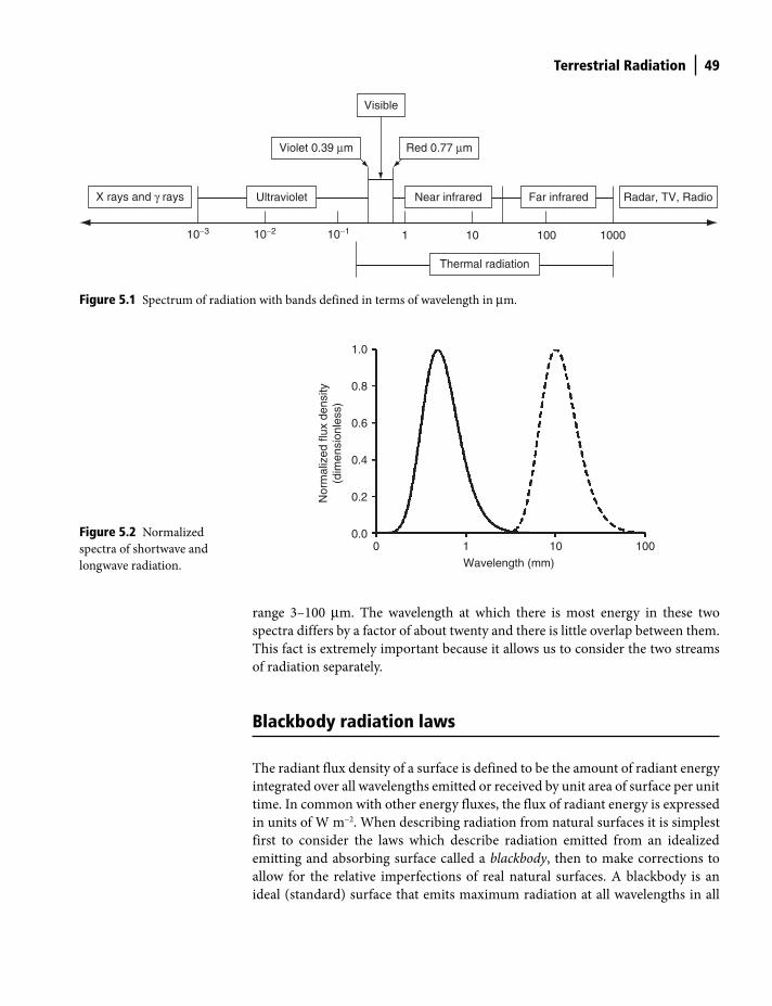
Terrestrial Radiation 49
range 3–100 μm. The wavelength at which there is most energy in these two
spectra differs by a factor of about twenty and there is little overlap between them.
This fact is extremely important because it allows us to consider the two streams
of radiation separately.
Blackbody radiation laws
The radiant flux density of a surface is defined to be the amount of radiant energy
integrated over all wavelengths emitted or received by unit area of surface per unit
time. In common with other energy fluxes, the flux of radiant energy is expressed
in units of W m−2. When describing radiation from natural surfaces it is simplest
first to consider the laws which describe radiation emitted from an idealized
emitting and absorbing surface called a blackbody, then to make corrections to
allow for the relative imperfections of real natural surfaces. A blackbody is an
ideal (standard) surface that emits maximum radiation at all wavelengths in all
00.0
0.2
0.4
0.6
1.0
0.8
1
Wavelength (mm)
Nor
mal
ized
flux
den
sity
(dim
ensi
onle
ss)
10 100Figure 5.2 Normalized
spectra of shortwave and
longwave radiation.
Figure 5.1 Spectrum of radiation with bands defined in terms of wavelength in μm.
10−3 10−2 10 100 100010−1 1
X rays and γ rays Ultraviolet Near infrared Far infrared Radar, TV, Radio
Thermal radiation
Violet 0.39 μm Red 0.77 μm
Visible
Shuttleworth_c05.indd 49Shuttleworth_c05.indd 49 11/3/2011 6:32:58 PM11/3/2011 6:32:58 PM
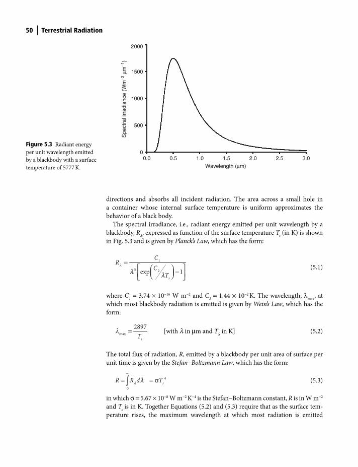
50 Terrestrial Radiation
directions and absorbs all incident radiation. The area across a small hole in
a container whose internal surface temperature is uniform approximates the
behavior of a black body.
The spectral irradiance, i.e., radiant energy emitted per unit wavelength by a
blackbody, Rl, expressed as function of the surface temperature Ts (in K) is shown
in Fig. 5.3 and is given by Planck’s Law, which has the form:
1
5 2exp 1s
CR
CT
=⎡ ⎤⎛ ⎞ −⎜ ⎟⎢ ⎥⎝ ⎠⎣ ⎦
l l
λ
(5.1)
where C1 = 3.74 × 10⁻¹⁶ W m−2 and C
2 = 1.44 × 10⁻² K. The wavelength, λ
max, at
which most blackbody radiation is emitted is given by Wein’s Law, which has the
form:
max
2897
sT=l
[with l in μm and TS in K] (5.2)
The total flux of radiation, R, emitted by a blackbody per unit area of surface per
unit time is given by the Stefan-Boltzmann Law, which has the form:
4
0
= sR R d T∞
= σ∫ l l (5.3)
in which σ = 5.67 × 10⁻⁸ W m−2 K−4 is the Stefan−Boltzmann constant, R is in W m−2
and Ts is in K. Together Equations (5.2) and (5.3) require that as the surface tem-
perature rises, the maximum wavelength at which most radiation is emitted
Figure 5.3 Radiant energy
per unit wavelength emitted
by a blackbody with a surface
temperature of 5777 K.
0.00
500
2000
1500
0.5 1.0
Wavelength (μm)
Spe
ctra
l irr
adia
nce
(Wm
−2 μ
m−1
)
2.0 2.5 3.01.5
1000
Shuttleworth_c05.indd 50Shuttleworth_c05.indd 50 11/3/2011 6:32:59 PM11/3/2011 6:32:59 PM
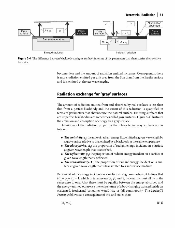
Terrestrial Radiation 51
becomes less and the amount of radiation emitted increases. Consequently, there
is more radiation emitted per unit area from the Sun than from the Earth’s surface
and it is emitted at shorter wavelengths.
Radiation exchange for ‘gray’ surfaces
The amount of radiation emitted from and absorbed by real surfaces is less than
that from a perfect blackbody and the extent of this reduction is quantified in
terms of parameters that characterize the natural surface. Emitting surfaces that
are imperfect blackbodies are sometimes called gray surfaces. Figure 5.4 illustrates
the emission and absorption of energy by a gray surface.
Definitions of the radiation properties that characterize gray surfaces are as
follows:
● The emissivity, e l: the ratio of radiant energy flux emitted at given wavelength by
a gray surface relative to that emitted by a blackbody at the same temperature.
● The absorptivity, a l: the proportion of radiant energy incident on a surface
at given wavelength that is absorbed.
● The reflectivity, r l: the proportion of radiant energy incident on a surface at
given wavelength that is reflected.
● The transmissivity, t l: the proportion of radiant energy incident on a sur-
face at given wavelength that is transmitted to a subsurface medium.
Because all of the energy incident on a surface must go somewhere, it follows that
(al + rl + tl) = 1, which in turn means al, rl and tl necessarily must all lie in the
range zero to one. Also, there must be equality between the energy absorbed and
the energy emitted otherwise the temperature of a body hanging isolated inside an
evacuated, isothermal container would rise or fall continuously. The Kirchoff ’s
Principle follows as a consequence of this and states that:
=l la e (5.4)
Greysurface
Greysurface
Emitted radiation Incident radiation
Same temperature
Blacksurface
All radiationabsorbed
R x ελ
R x αλ R x τλ
R x ρλR
R R
Blacksurface
Figure 5.4 The difference between blackbody and gray surfaces in terms of the parameters that characterize their relative
behavior.
Shuttleworth_c05.indd 51Shuttleworth_c05.indd 51 11/3/2011 6:33:02 PM11/3/2011 6:33:02 PM
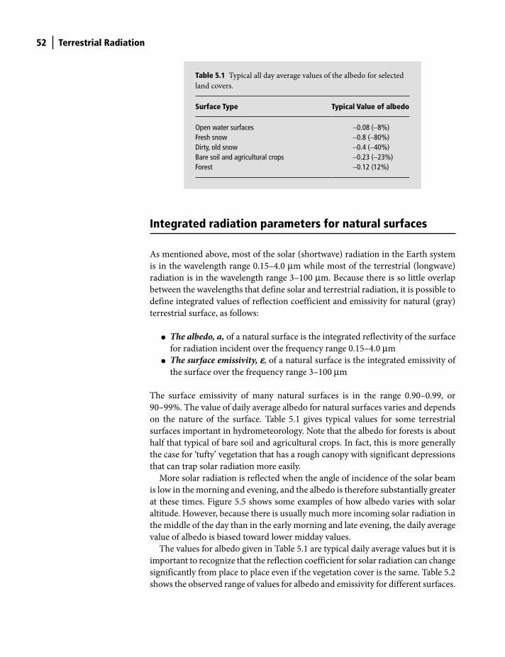
52 Terrestrial Radiation
Integrated radiation parameters for natural surfaces
As mentioned above, most of the solar (shortwave) radiation in the Earth system
is in the wavelength range 0.15–4.0 μm while most of the terrestrial (longwave)
radiation is in the wavelength range 3–100 μm. Because there is so little overlap
between the wavelengths that define solar and terrestrial radiation, it is possible to
define integrated values of reflection coefficient and emissivity for natural (gray)
terrestrial surface, as follows:
● The albedo, a, of a natural surface is the integrated reflectivity of the surface
for radiation incident over the frequency range 0.15–4.0 μm
● The surface emissivity, e, of a natural surface is the integrated emissivity of
the surface over the frequency range 3–100 μm
The surface emissivity of many natural surfaces is in the range 0.90–0.99, or
90–99%. The value of daily average albedo for natural surfaces varies and depends
on the nature of the surface. Table 5.1 gives typical values for some terrestrial
surfaces important in hydrometeorology. Note that the albedo for forests is about
half that typical of bare soil and agricultural crops. In fact, this is more generally
the case for ‘tufty’ vegetation that has a rough canopy with significant depressions
that can trap solar radiation more easily.
More solar radiation is reflected when the angle of incidence of the solar beam
is low in the morning and evening, and the albedo is therefore substantially greater
at these times. Figure 5.5 shows some examples of how albedo varies with solar
altitude. However, because there is usually much more incoming solar radiation in
the middle of the day than in the early morning and late evening, the daily average
value of albedo is biased toward lower midday values.
The values for albedo given in Table 5.1 are typical daily average values but it is
important to recognize that the reflection coefficient for solar radiation can change
significantly from place to place even if the vegetation cover is the same. Table 5.2
shows the observed range of values for albedo and emissivity for different surfaces.
Table 5.1 Typical all day average values of the albedo for selected
land covers.
Surface Type Typical Value of albedo
Open water surfaces ∼0.08 (∼8%)Fresh snow ∼0.8 (∼80%)Dirty, old snow ∼0.4 (∼40%)Bare soil and agricultural crops ∼0.23 (∼23%)Forest ∼0.12 (12%)
Shuttleworth_c05.indd 52Shuttleworth_c05.indd 52 11/3/2011 6:33:03 PM11/3/2011 6:33:03 PM
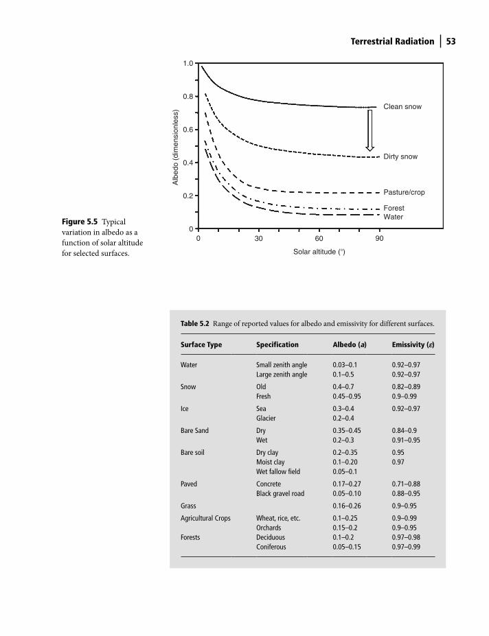
Terrestrial Radiation 53
Figure 5.5 Typical
variation in albedo as a
function of solar altitude
for selected surfaces.
00
0.2
Clean snow
Dirty snow
Pasture/crop
ForestWater
0.4
0.6
0.8
1.0
30 60
Solar altitude (�)
Alb
edo
(dim
ensi
onle
ss)
90
Table 5.2 Range of reported values for albedo and emissivity for different surfaces.
Surface Type Specification Albedo (a) Emissivity (e)
Water Small zenith angle 0.03–0.1 0.92–0.97Large zenith angle 0.1–0.5 0.92–0.97
Snow Old 0.4–0.7 0.82–0.89Fresh 0.45–0.95 0.9–0.99
Ice Sea 0.3–0.4 0.92–0.97Glacier 0.2–0.4
Bare Sand Dry 0.35–0.45 0.84–0.9Wet 0.2–0.3 0.91–0.95
Bare soil Dry clay 0.2–0.35 0.95Moist clay 0.1–0.20 0.97Wet fallow field 0.05–0.1
Paved Concrete 0.17–0.27 0.71–0.88Black gravel road 0.05–0.10 0.88–0.95
Grass 0.16–0.26 0.9–0.95
Agricultural Crops Wheat, rice, etc. 0.1–0.25 0.9–0.99Orchards 0.15–0.2 0.9–0.95
Forests Deciduous 0.1–0.2 0.97–0.98 Coniferous 0.05–0.15 0.97–0.99
Shuttleworth_c05.indd 53Shuttleworth_c05.indd 53 11/3/2011 6:33:03 PM11/3/2011 6:33:03 PM

54 Terrestrial Radiation
The value of the albedo also strongly depends on the altitude of the Sun and so
varies through the day.
The reflection coefficient for electromagnetic radiation incident on land sur-
faces in the solar waveband changes with the wavelength of the radiation and this
behavior is important both in the context of remote sensing and when building
numerical models of land surface exchanges. Figure 5.6 shows examples of the
variation in reflection coefficient with wavelength for fresh green vegetation, dry
(dead) vegetation, and soil. The reflection coefficient for soil changes with wave-
length, but in a much less dramatic way than it does for green leaves. The distinct
change in the reflection coefficient for plant leaves above and below about
0.72 μm is associated with the absorption of Photosynthetically Active Radiation
(PAR), i.e., that portion of incoming solar radiation that plants use to provide the
energy they need to carry out photosynthesis. In Fig. 5.6, for example, the ratio of
the reflection coefficient at 0.65 and 0.85 μm is about 1.2 for soil and about 1.5 for
dry (dead leaves) but is much greater for actively transpiring green leaves. Some
remote sensing systems measure the relative reflection coefficient at selected wave-
lengths above and below 0.72 μm and use this distinct difference in the ratio of the
measured reflection coefficients to diagnose the extent to which vegetation covers
the soil beneath. The difference in reflection coefficient for leaves above and below
0.72 μm is so distinct that some advanced models of land surface exchanges also
choose to recognize it in their computations and they separately model the absorp-
tion and reflection of visible light in wavebands below and above this wavelength.
Maximum solar radiation at the top of atmosphere
As mentioned earlier, the flux of solar energy at all wavelengths incident on unit
area normal to solar beam at the outer edge of atmosphere when the Earth is at its
mean distance (one astronomical unit) is called the ‘solar constant’, So. In fact the
Figure 5.6 Typical
variation of spectral
reflectance with wavelength
for green vegetation, dry
(dead) vegetation, and soil.
0.5
Green vegetation
Dry vegetation
Soil
0.0
0.2
0.4
0.6
1.0
Wavelength (μm)
Ref
lect
ance
(di
men
sion
less
)
1.5 2.0 2.5
Shuttleworth_c05.indd 54Shuttleworth_c05.indd 54 11/3/2011 6:33:04 PM11/3/2011 6:33:04 PM
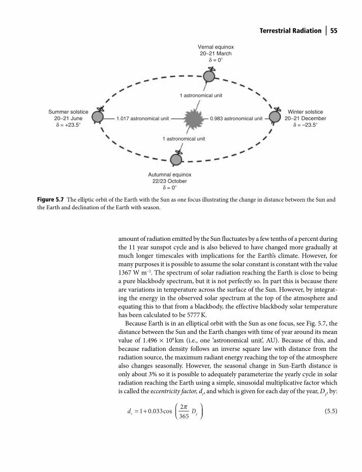
Terrestrial Radiation 55
amount of radiation emitted by the Sun fluctuates by a few tenths of a percent during
the 11 year sunspot cycle and is also believed to have changed more gradually at
much longer timescales with implications for the Earth’s climate. However, for
many purposes it is possible to assume the solar constant is constant with the value
1367 W m−2. The spectrum of solar radiation reaching the Earth is close to being
a pure blackbody spectrum, but it is not perfectly so. In part this is because there
are variations in temperature across the surface of the Sun. However, by integrat-
ing the energy in the observed solar spectrum at the top of the atmosphere and
equating this to that from a blackbody, the effective blackbody solar temperature
has been calculated to be 5777 K.
Because Earth is in an elliptical orbit with the Sun as one focus, see Fig. 5.7, the
distance between the Sun and the Earth changes with time of year around its mean
value of 1.496 × 10⁸ km (i.e., one ‘astronomical unit’, AU). Because of this, and
because radiation density follows an inverse square law with distance from the
radiation source, the maximum radiant energy reaching the top of the atmosphere
also changes seasonally. However, the seasonal change in Sun-Earth distance is
only about 3% so it is possible to adequately parameterize the yearly cycle in solar
radiation reaching the Earth using a simple, sinusoidal multiplicative factor which
is called the eccentricity factor, dr, and which is given for each day of the year, D
y, by:
21 0.033cos
365r yd D⎛ ⎞= + ⎜ ⎟⎝ ⎠
p (5.5)
Figure 5.7 The elliptic orbit of the Earth with the Sun as one focus illustrating the change in distance between the Sun and
the Earth and declination of the Earth with season.
Autumnal equinox22/23 October
δ = 0�
Vernal equinox20−21 March
δ = 0�
Winter solstice20−21 December
δ = –23.5�
Summer solstice20−21 Juneδ = +23.5�
1 astronomical unit
1 astronomical unit
1.017 astronomical unit 0.983 astronomical unit
Shuttleworth_c05.indd 55Shuttleworth_c05.indd 55 11/3/2011 6:33:04 PM11/3/2011 6:33:04 PM
56 Terrestrial Radiation
Consequently, the energy reaching the top of the atmosphere as solar radiation
normal to the solar beam is calculated by:
top r oS d S= (5.6)
D is the day of the year (sometimes inaccurately called the Julian day), with D = 1
on 1 January and D = 365 on 31 December.
Maximum solar radiation at the ground
The starting point for calculating how much solar energy reaches the ground is to
calculate the energy that would reach the surface if there were no intervening
atmosphere. The amount of solar radiation which would be received per unit area
over a specified time interval t1 to t
2 on a horizontal surface on Earth were there no
intervening atmosphere is called the insolation, I, which is calculated from:
= ∫1
2
cos( ).
t
o rt
I S d dtq (5.7)
where q is the solar zenith angle, i.e., the apparent angle of the Sun relative to the
normal angle to the surface at the specific location.
The need is, therefore, to calculate the solar zenith angle. Doing this is complex,
because the solar zenith angle depends not only on the latitude of the site for
which the calculation is made (because the Sun is on average closer to overhead
nearer the equator), and the time of day (because the Earth rotates each day), but
also because it depends on the solar declination, d. The solar declination is the
angle between the rays of the Sun and the plane of the Earth’s equator. The axis of
rotation of the Earth is at an angle of ∼23.5° with respect to the plane in which the
Earth moves around the Sun, see Fig. 5.7. Consequently, the solar declination
changes with time of year. It is zero at the vernal and autumnal equinox, and
around 23.5° and -23.5° at the summer and winter solstice, respectively. The value
of δ can be calculated (in radians) for each day of the year, Dy, from:
20.4093sin 1.405
365yD
⎛ ⎞= −⎜ ⎟⎝ ⎠pd (5.8)
For a site at latitude f (positive in the northern hemisphere; negative in the southern
hemisphere), the cosine of the solar zenith angle required in Equation (5.7) to
calculate the insolation is given by:
cos sin sin cos cos cos= +q f d f d ω (5.9)
Shuttleworth_c05.indd 56Shuttleworth_c05.indd 56 11/3/2011 6:33:05 PM11/3/2011 6:33:05 PM
Terrestrial Radiation 57
where w is the hour angle, i.e., the angle representing time of day, which is given by:
( )12 (in radians)
12
h−= πw (5.10)
where h is time of day in hours in local time. Thus, if there were no atmosphere, on a
particular day the daily total incoming solar energy received at the ground integrated
over daylight hours between t1 and t
2, i.e., the daily insolation I
o, is given by:
= +∫2
1
(sin sin cos cos cos )o
t
o rt
I S d dtf d f d w (5.11)
The values of t1 and t
2 are best expressed in terms of the equivalent hour angle that
defines both the beginning and end of the day. This angle is called the sunset hour
angle, ws, which can be calculated from;
arccos ( tan tan ) [radians]s = −w f d (5.12)
with the day length, N, in hours then following immediately from:
= 24 [hours]sN wp (5.13)
The total solar energy which would be received per unit area between sunrise and
sunset on a horizontal surface at latitude f if there were no intervening atmos-
phere is then obtained by integrating Equation (5.11) between -ws and +w
s as:
2 1
037.7 ( sin sin cos cos sin ) [ MJ m d ]d
r s sS d − −= +w wf d f d (5.14)
where dr, d, and w
s are given by Equations (5.5), (5.8), and (5.12), respectively. When
estimating evaporation rates, it is sometimes convenient to write Equation (5.14)
in terms of an equivalent depth of evaporated water, thus:
1
015.39 ( sin sin cos cos sin ) [ mm d ]d
r s sS d −= +φ δ φ δ ωw (5.15)
It is important when estimating daily average evaporation rates (see Chapter 23)
that this absolute upper limit on evaporation rate (from which estimates of actual
evaporation rates can be made) can always be calculated solely on the basis of
knowledge of the latitude of the site and the day of the year.
Shuttleworth_c05.indd 57Shuttleworth_c05.indd 57 11/3/2011 6:33:09 PM11/3/2011 6:33:09 PM
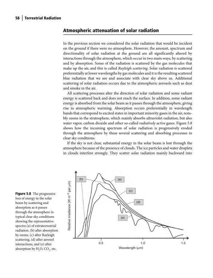
58 Terrestrial Radiation
Atmospheric attenuation of solar radiation
In the previous section we considered the solar radiation that would be incident
on the ground if there were no atmosphere. However, the amount, spectrum and
directionality of solar radiation at the ground are all significantly altered by
interactions through the atmosphere, which occur in two main ways, by scattering
and by absorption. Some of the radiation is scattered by the gas molecules that
make up the air, and this is called Rayleigh scattering. Solar radiation is scattered
preferentially at lower wavelengths by gas molecules and it is the resulting scattered
blue radiation that we see and associate with clear sky above us. Additional
scattering of solar radiation occurs due to the atmospheric aerosols such as dust
and smoke in the air.
All scattering processes alter the direction of solar radiation and some radiant
energy is scattered back and does not reach the surface. In addition, some radiant
energy is absorbed from the solar beam as it passes through the atmosphere, giving
rise to atmospheric warming. Absorption occurs preferentially in wavelength
bands that correspond to excited states in important minority gases in the air, nota-
bly ozone in the stratosphere, which mainly absorbs ultraviolet radiation, but also
water vapor, carbon dioxide and other so-called radiatively active gases. Figure 5.8
shows how the incoming spectrum of solar radiation is progressively eroded
through the atmosphere by these several scattering and absorbing processes in
clear sky conditions.
If the sky is not clear, substantial energy in the solar beam is lost through the
atmosphere because of the presence of clouds. The ice particles and water droplets
in clouds interfere strongly. They scatter solar radiation mainly backward into
Figure 5.8 The progressive
loss of energy in the solar
beam by scattering and
absorption as it passes
through the atmosphere in
typical clear sky conditions
showing the representative
spectra (a) of extraterrestrial
radiation, (b) after absorption
by ozone, (c) after Rayleigh
scattering, (d) after aerosol
interactions, and (e) after
absorption by H2O, CO
2, etc.
0.5
(e)
(d)
(c)
(a)(b)
Rel
ativ
e irr
adie
nce
(W m
−2 p
er μ
m)
1.0
Wavelength (μm)
1.5
Shuttleworth_c05.indd 58Shuttleworth_c05.indd 58 11/3/2011 6:33:15 PM11/3/2011 6:33:15 PM
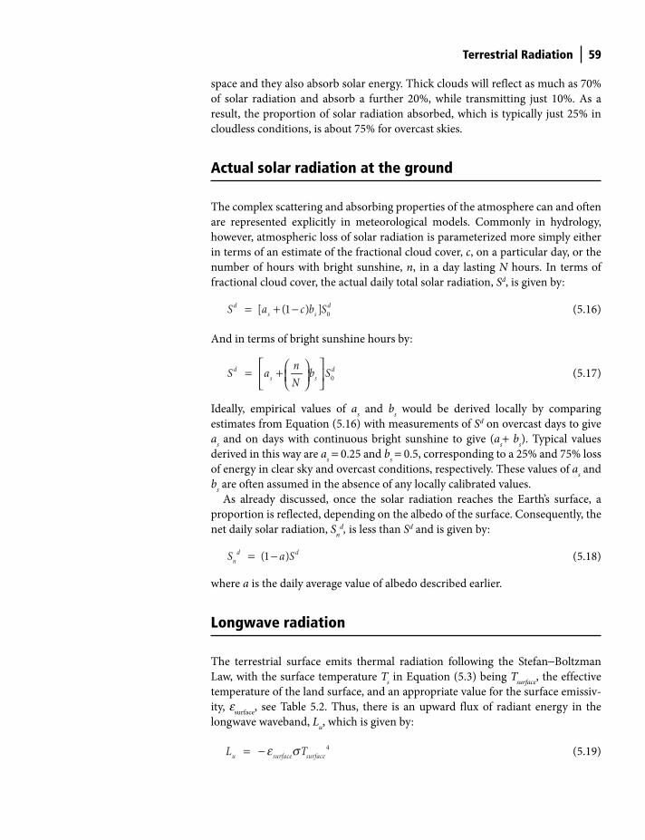
Terrestrial Radiation 59
space and they also absorb solar energy. Thick clouds will reflect as much as 70%
of solar radiation and absorb a further 20%, while transmitting just 10%. As a
result, the proportion of solar radiation absorbed, which is typically just 25% in
cloudless conditions, is about 75% for overcast skies.
Actual solar radiation at the ground
The complex scattering and absorbing properties of the atmosphere can and often
are represented explicitly in meteorological models. Commonly in hydrology,
however, atmospheric loss of solar radiation is parameterized more simply either
in terms of an estimate of the fractional cloud cover, c, on a particular day, or the
number of hours with bright sunshine, n, in a day lasting N hours. In terms of
fractional cloud cover, the actual daily total solar radiation, Sd, is given by:
0 [ (1 ) ]d d
s sS a c b S= + − (5.16)
And in terms of bright sunshine hours by:
0 d d
s snS a b SN
⎡ ⎤⎛ ⎞= +⎢ ⎥⎜ ⎟⎝ ⎠⎣ ⎦ (5.17)
Ideally, empirical values of as and b
s would be derived locally by comparing
estimates from Equation (5.16) with measurements of Sd on overcast days to give
as and on days with continuous bright sunshine to give (a
s+ b
s). Typical values
derived in this way are as = 0.25 and b
s = 0.5, corresponding to a 25% and 75% loss
of energy in clear sky and overcast conditions, respectively. These values of as and
bs are often assumed in the absence of any locally calibrated values.
As already discussed, once the solar radiation reaches the Earth’s surface, a
proportion is reflected, depending on the albedo of the surface. Consequently, the
net daily solar radiation, Sn
d, is less than Sd and is given by:
(1 )d dnS a S= − (5.18)
where a is the daily average value of albedo described earlier.
Longwave radiation
The terrestrial surface emits thermal radiation following the Stefan−Boltzman
Law, with the surface temperature Ts in Equation (5.3) being T
surface, the effective
temperature of the land surface, and an appropriate value for the surface emissiv-
ity, esurface
, see Table 5.2. Thus, there is an upward flux of radiant energy in the
longwave waveband, Lu, which is given by:
4 u surface surfaceL T= - e s (5.19)
Shuttleworth_c05.indd 59Shuttleworth_c05.indd 59 11/3/2011 6:33:15 PM11/3/2011 6:33:15 PM
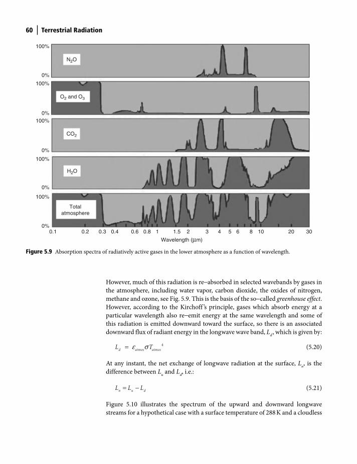
60 Terrestrial Radiation
However, much of this radiation is re−absorbed in selected wavebands by gases in
the atmosphere, including water vapor, carbon dioxide, the oxides of nitrogen,
methane and ozone, see Fig. 5.9. This is the basis of the so−called greenhouse effect.
However, according to the Kirchoff ’s principle, gases which absorb energy at a
particular wavelength also re−emit energy at the same wavelength and some of
this radiation is emitted downward toward the surface, so there is an associated
downward flux of radiant energy in the longwave wave band, Ld , which is given by:
4 d atmos atmosL T= ε s (5.20)
At any instant, the net exchange of longwave radiation at the surface, Ln, is the
difference between Lu and L
d, i.e.:
n u dL L L= − (5.21)
Figure 5.10 illustrates the spectrum of the upward and downward longwave
streams for a hypothetical case with a surface temperature of 288 K and a cloudless
Figure 5.9 Absorption spectra of radiatively active gases in the lower atmosphere as a function of wavelength.
0.10%
0%
0%
100%
100%
0%100%
0%
100%
N2O
H2O
Totalatmosphere
O2 and O3
CO2
100%
0.2 0.3 0.4 0.6 0.8 1.51 2
Wavelength (μm)
3 4 5 6 8 10 20 30
Shuttleworth_c05.indd 60Shuttleworth_c05.indd 60 11/3/2011 6:33:19 PM11/3/2011 6:33:19 PM
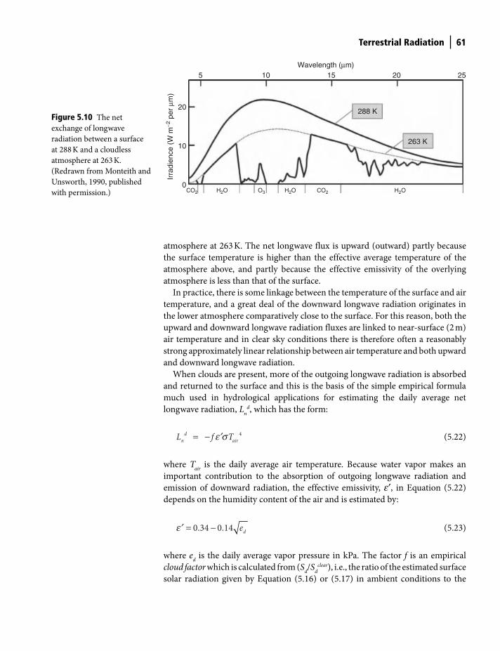
Terrestrial Radiation 61
atmosphere at 263 K. The net longwave flux is upward (outward) partly because
the surface temperature is higher than the effective average temperature of the
atmosphere above, and partly because the effective emissivity of the overlying
atmosphere is less than that of the surface.
In practice, there is some linkage between the temperature of the surface and air
temperature, and a great deal of the downward longwave radiation originates in
the lower atmosphere comparatively close to the surface. For this reason, both the
upward and downward longwave radiation fluxes are linked to near-surface (2 m)
air temperature and in clear sky conditions there is therefore often a reasonably
strong approximately linear relationship between air temperature and both upward
and downward longwave radiation.
When clouds are present, more of the outgoing longwave radiation is absorbed
and returned to the surface and this is the basis of the simple empirical formula
much used in hydrological applications for estimating the daily average net
longwave radiation, Ln
d, which has the form:
4 dn airL f T= − e¢s (5.22)
where Tair
is the daily average air temperature. Because water vapor makes an
important contribution to the absorption of outgoing longwave radiation and
emission of downward radiation, the effective emissivity, e′, in Equation (5.22)
depends on the humidity content of the air and is estimated by:
0.34 0.14 de= −e¢ (5.23)
where ed is the daily average vapor pressure in kPa. The factor f is an empirical
cloud factor which is calculated from (Sd/S
dclear), i.e., the ratio of the estimated surface
solar radiation given by Equation (5.16) or (5.17) in ambient conditions to the
Figure 5.10 The net
exchange of longwave
radiation between a surface
at 288 K and a cloudless
atmosphere at 263 K.
(Redrawn from Monteith and
Unsworth, 1990, published
with permission.)0
5 10 15 20
288 K
263 K
25Wavelength (μm)
Irra
dien
ce (
W m
−2 p
er μ
m)
10
20
CO2 CO2O3H2O H2O H2O
Shuttleworth_c05.indd 61Shuttleworth_c05.indd 61 11/3/2011 6:33:22 PM11/3/2011 6:33:22 PM

62 Terrestrial Radiation
value estimated by the same equation for clear sky conditions. Two empirical
formulae are used to calculate f, one applicable in humid conditions and one in
arid conditions. In humid conditions:
( )(1 ) i.e., ; or
ds ss s
ds s s sclear
a n N ba c bSfa b a bS
+⎛ ⎞ ⎡ ⎤+ −= ⎢ ⎥⎜ ⎟ + +⎝ ⎠ ⎣ ⎦
(5.24)
but in arid conditions:
(5.25)
Net radiation at the surface
As described in Chapter 2, the all−day average net radiation at the surface is the
sum of the downward and reflected solar radiation and the net longwave radia-
tion as illustrated in Figure 4.2, and the daily average net radiation flux, Rn
d, is
given by:
d d dn n nR S L= + (5.26)
Equation (5.26) is written in terms of daily total values but it is of course possible
to write equations describing the instantaneous radiation balance, as follows:
( ) ( )n r d uR S S L L= + + + (5.27)
or:
(1 )n nR S a L= − + (5.28)
The value of Rn varies greatly through the day. Net longwave radiation is negative
and usually fairly constant through the day, with the net solar radiation provid-
ing a positive input during the daylight hours. The typical diurnal cycle of net
radiation therefore has a temperature dependent negative offset, upon which is
superimposed a positive diurnal input of solar radiation whose magnitude
depends on the latitude of the site, the day of the year, fractional cloud cover on
that day, and, not least, time of day. The resulting diurnal pattern of net radiation
may therefore have a strong seasonal dependence at high latitude as illustrated
in the case of the radiation balance for Bergen, Norway at 60°N, which is shown
in Fig. 5.11.
+⎛ ⎞ ⎡ ⎤+ −= − − −⎢ ⎥⎜ ⎟ + +⎝ ⎠ ⎣ ⎦
( )(1 )1.35 0.35 i.e., 1.35 0.35; or,1.35 0.35
ds ss s
ds s s sclear
a n N ba c bSfa b a bS
Shuttleworth_c05.indd 62Shuttleworth_c05.indd 62 11/3/2011 6:33:24 PM11/3/2011 6:33:24 PM
Terrestrial Radiation 63
Height dependence of net radiation
The main focus of interest in this chapter is on radiation exchange at terrestrial
surfaces. However, when considering the energy balance of the atmospheric
boundary layer, it is important to recognize that net radiation can change with
height above the ground. This is inevitable because there is absorption of solar
radiation as it passes through the air, and there is absorption and emission of long-
wave radiation at all levels in the atmosphere. During the day, solar radiation
Figure 5.11 Diurnal variation in net solar radiation, upward and downward radiation, and net radiation at Bergen Norway
on (a) 13 April 1968 and (b) 11 January 1968. (Redrawn from Monteith and Unsworth, 1990; after Gates, 1980, published
with permission.)
00
–100
Rad
iatio
n flu
x (W
m−2
)
200
400
600
0
03 06 09 12 15 18 21 24
Netradiation
Netradiation
Upward longwaveradiation
Upward longwaveradiation
(a)
Solarradiation
Solarradiation
Downward longwaveradiation
Downward longwaveradiation
Local time (hr)
00
–100
Rad
iatio
n flu
x (W
m−2
)
200
400
0
03 06 09 12 15 18 21 24
(b)
Local time (hr)
Shuttleworth_c05.indd 63Shuttleworth_c05.indd 63 11/3/2011 6:33:28 PM11/3/2011 6:33:28 PM
64 Terrestrial Radiation
normally dominates the net radiation flux and in the absence of cloud, fog, or
heavy aerosol contamination, the loss of solar radiation through the clear air
boundary layer is comparatively small. The profile of longwave radiation through
the boundary layer can be influenced by variations in the concentration of radia-
tively active atmospheric constituents and the heat content of the air. During the
night, longwave radiation dominates and the nighttime potential temperature
profile may induce vertical changes in the net radiation flux. Regardless of its
cause, energy conservation means vertical divergence of the net radiation flux will
be associated with local heating or cooling of the air, the amount being directly
related to the rate of change of net radiation with height and given by:
v np
Rc
t z∂ ∂
=∂ ∂q
r (5.29)
Important points in this chapter
● Separation of wavebands: most solar radiation is in the wavelength range
0.15–4 μm and most longwave radiation in the Earth system is in the wave-
length range 3–100 μm, this allows separate consideration of the two streams.
● Blackbody radiation laws: describe radiation for an idealized emitting and
absorbing blackbody surface, and include Planck’s Law describing the
spectrum; Wein’s Law, giving the wavelength of peak emission; and Stefan-
Boltzmann Law, giving the total flux of radiation.
● Gray surfaces: are imperfect blackbodies for which radiation exchange at
wavelength l is calculated from blackbody radiation using multiplicative
factors, i.e., emissivity (el) for emitted radiant energy; absorptivity (al) for
absorbed radiant energy, reflectivity (rl), for emitted radiant energy; and
transmissivity (tl) for transmitted radiant energy. Kirchov’s principle requires
that el = al.
● Integrated parameters for natural surfaces: because there is little overlap
between the waveband for solar and longwave radiation, radiation exchange
for natural surfaces is often described by wavelength integrated surface
properties, i.e., albedo (a), the integrated reflectivity for solar radiation, and
emissivity (e), the integrated emissivity for longwave radiation.
● Typical values of parameters: daily average values albedo are typically ∼8%
for water, ∼80% for fresh and ∼40% for dirty snow, ∼23% for bare soil and
agricultural crops, and ∼12% for forests; emissivity is typically ∼95 ± 5%.
● Top of atmosphere solar radiation: maximum value changes by about ±1.6%
with day of year around the ‘solar constant’ So = 1367 W m−2.
● Maximum solar radiation at the ground: if there were no atmosphere the
daily total solar radiation reaching the ground could be calculated using
an (albeit complex) formula from the latitude of the site (f), solar declination
Shuttleworth_c05.indd 64Shuttleworth_c05.indd 64 11/3/2011 6:33:29 PM11/3/2011 6:33:29 PM
Terrestrial Radiation 65
(d – a function of day of year), and the sunset hour angle, (ws – a function of
latitude and day of year).
● Atmospheric attenuation: typically 25% of solar radiation is absorbed for
clear skies and 75% for overcast skies (attenuation is by scattering by gas
molecules and dust, and absorption by radiatively active gases and cloud):
solar radiation at the ground can be estimated either from fractional cloud
cover or from the fraction of daytime hours with bright sunshine.
● Net longwave radiation: longwave exchange with the surface can be
estimated using a version of the Stefan-Boltzmann Law that includes an
effective emissivity (dependent on humidity) and a cloud cover correction
factor (estimated from the attenuation of solar radiation) that is different for
humid and arid conditions.
● Net radiation: is obtained by adding the net solar radiation (allowing for
albedo) to the net longwave radiation; at the daily time scale it has a tempera-
ture dependent negative (longwave) offset upon which is superimposed a
positive solar radiation input whose magnitude depends on latitude, day of
the year, fractional cloud cover, and time of day.
References
Gates, D.M. (1980) Biophysical Ecology. Springer-Verlag, New York.
Monteith, J.L. & Unsworth, M.H. (1990) Principles of Environmental Physics. Edward
Arnold, London, UK.
Shuttleworth_c05.indd 65Shuttleworth_c05.indd 65 11/3/2011 6:33:30 PM11/3/2011 6:33:30 PM
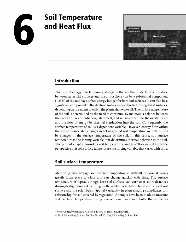
Introduction
The flow of energy into temporary storage in the soil that underlies the interface
between terrestrial surfaces and the atmosphere can be a substantial component
(∼25%) of the midday surface energy budget for bare soil surfaces. It can also be a
significant component of the daytime surface energy budget for vegetated surfaces,
depending on the extent to which the plants shade the soil. The surface temperature
of the soil is determined by the need to continuously maintain a balance between
the energy fluxes of radiation, latent heat, and sensible heat into the overlying air
and the flow of energy by thermal conduction into the soil. Consequently, the
surface temperature of soil is a dependent variable. However, energy flow within
the soil and associated changes in below ground soil temperature are determined
by changes in the surface temperature of the soil. In this sense, soil surface
temperature is the forcing variable that determines thermal behavior in the soil.
The present chapter considers soil temperatures and heat flow in soil from the
perspective that soil surface temperature is a forcing variable that varies with time.
Soil surface temperature
Measuring area-average soil surface temperature is difficult because it varies
greatly from place to place and can change quickly with time. The surface
temperature of typically rough bare soil surfaces can vary over short distances
during daylight hours depending on the relative orientation between the local soil
surface and the solar beam. Spatial variability in plant shading complicates this
relationship for soil covered by vegetation. Attempts have been made to measure
soil surface temperature using conventional mercury bulb thermometers
6 Soil Temperature and Heat Flux
Terrestrial Hydrometeorology, First Edition. W. James Shuttleworth.
© 2012 John Wiley & Sons, Ltd. Published 2012 by John Wiley & Sons, Ltd.
Shuttleworth_c06.indd 66Shuttleworth_c06.indd 66 11/3/2011 6:32:11 PM11/3/2011 6:32:11 PM
Soil Temperature and Heat Flux 67
positioned to be in close contact with the soil. But the presence of a thermometer
alters the surface energy balance and therefore the surface temperature that is
being measured. Fine thermocouple thermometers positioned on the soil surface
disturb the surface energy balance less, but the issue of how to obtain an adequate
sample to determine the area-average temperature remains. In principle, the
average temperature can be measured over areas of a few square meters of soil by
positioning a radiometer above it and deducing the surface temperature from the
measured thermal radiation emitted. However, soil surfaces are not blackbody
emitters so soil emissivity has to be assumed and poor knowledge of this can
systematically bias such a radiometric measurement by several degrees.
The soil surface temperature is determined by the surface energy balance. As a
result, for dry exposed soils in fairly calm conditions and with clear skies, the ampli-
tude of the daily cycle in soil surface temperature can be very large, perhaps greater
than 30°C. This is noticeably larger, by perhaps a factor of two, than the daily cycle
in air temperature measured at 2 m. Incoming radiant energy plays a major role in
the surface energy balance that determines the surface temperature of bare soil and
the timing of the daily cycle in soil temperature, therefore, tends to follow that in
net radiation, albeit with some lag (typically less than an hour). For a wet soil surface,
much of the energy outgoing to the atmosphere is as latent heat and the sensible heat
flux is less. There is, therefore, less need for a large difference in temperature between
the soil surface and the overlying air to support the sensible heat flux. Consequently,
the amplitude of the daily cycle in soil surface temperature is much smaller. But solar
radiation is still the dominant term in available energy for wet bare soil so the timing
of the daily cycle in soil temperature still tends to follow that in net radiation.
When there is vegetation overlying the soil, the magnitude and timing of the
daily cycle in soil surface temperature differs from that for bare soil. Much of
the incoming radiant energy is captured by the vegetation canopy and returned to
the atmosphere before it reaches the soil. The presence of vegetation also enhances
turbulent mixing in the air near the ground thus reducing the difference in
temperature between air adjacent to the soil surface and that in the atmosphere
above. Since there is much less solar radiation reaching the soil surface, the solar
cycle has less influence on surface energy balance and soil surface temperature, the
latter being thus more similar to near-surface air temperature. Consequently, the
daily cycle in vegetation-covered soil surface temperature has reduced amplitude
relative to that for bare soil in the same meteorological conditions, and the timing
of the cycle tends to follow that in air temperature and so typically lags the solar
radiation cycle by several hours.
Subsurface soil temperatures
The temperature of soil below the surface is somewhat easier to measure than
soil surface temperature providing the thermometers are carefully inserted with
minimum disturbance to the soil structure. Commonly, small thermometers are
Shuttleworth_c06.indd 67Shuttleworth_c06.indd 67 11/3/2011 6:32:12 PM11/3/2011 6:32:12 PM
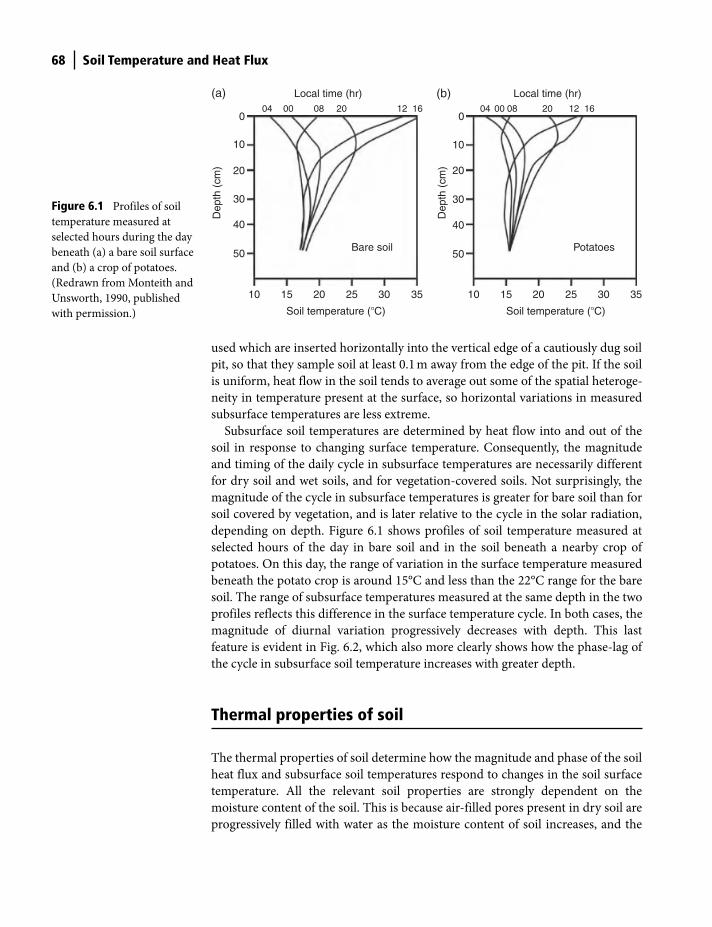
68 Soil Temperature and Heat Flux
used which are inserted horizontally into the vertical edge of a cautiously dug soil
pit, so that they sample soil at least 0.1 m away from the edge of the pit. If the soil
is uniform, heat flow in the soil tends to average out some of the spatial heteroge-
neity in temperature present at the surface, so horizontal variations in measured
subsurface temperatures are less extreme.
Subsurface soil temperatures are determined by heat flow into and out of the
soil in response to changing surface temperature. Consequently, the magnitude
and timing of the daily cycle in subsurface temperatures are necessarily different
for dry soil and wet soils, and for vegetation-covered soils. Not surprisingly, the
magnitude of the cycle in subsurface temperatures is greater for bare soil than for
soil covered by vegetation, and is later relative to the cycle in the solar radiation,
depending on depth. Figure 6.1 shows profiles of soil temperature measured at
selected hours of the day in bare soil and in the soil beneath a nearby crop of
potatoes. On this day, the range of variation in the surface temperature measured
beneath the potato crop is around 15°C and less than the 22°C range for the bare
soil. The range of subsurface temperatures measured at the same depth in the two
profiles reflects this difference in the surface temperature cycle. In both cases, the
magnitude of diurnal variation progressively decreases with depth. This last
feature is evident in Fig. 6.2, which also more clearly shows how the phase-lag of
the cycle in subsurface soil temperature increases with greater depth.
Thermal properties of soil
The thermal properties of soil determine how the magnitude and phase of the soil
heat flux and subsurface soil temperatures respond to changes in the soil surface
temperature. All the relevant soil properties are strongly dependent on the
moisture content of the soil. This is because air-filled pores present in dry soil are
progressively filled with water as the moisture content of soil increases, and the
40
50
30
20
10
0
Dep
th (
cm)
10 15 20 25 30 35
04 00 08 20 12 16
Local time (hr)
Bare soil
Soil temperature (�C)
(a)
40
50
10 15 20 25 30 35
30
20
10
004 00 08 20 12 16
Local time (hr)
Potatoes
Dep
th (
cm)
Soil temperature (�C)
(b)
Figure 6.1 Profiles of soil
temperature measured at
selected hours during the day
beneath (a) a bare soil surface
and (b) a crop of potatoes.
(Redrawn from Monteith and
Unsworth, 1990, published
with permission.)
Shuttleworth_c06.indd 68Shuttleworth_c06.indd 68 11/3/2011 6:32:12 PM11/3/2011 6:32:12 PM
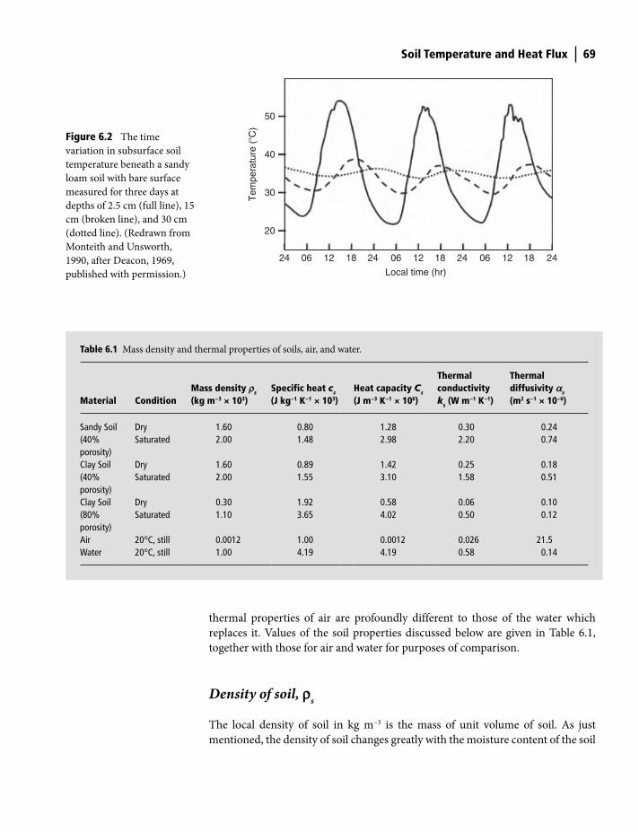
Soil Temperature and Heat Flux 69
thermal properties of air are profoundly different to those of the water which
replaces it. Values of the soil properties discussed below are given in Table 6.1,
together with those for air and water for purposes of comparison.
Density of soil, rs
The local density of soil in kg m−3 is the mass of unit volume of soil. As just
mentioned, the density of soil changes greatly with the moisture content of the soil
24 06 12 18 24 06 12
Local time (hr)
18 24 06 12 18 24
20
30
40
50
Tem
pera
ture
(�C
)
Figure 6.2 The time
variation in subsurface soil
temperature beneath a sandy
loam soil with bare surface
measured for three days at
depths of 2.5 cm (full line), 15
cm (broken line), and 30 cm
(dotted line). (Redrawn from
Monteith and Unsworth,
1990, after Deacon, 1969,
published with permission.)
Table 6.1 Mass density and thermal properties of soils, air, and water.
Material ConditionMass density rs (kg m−3 × 10³)
Specific heat cs (J kg−1 K−1 × 10³)
Heat capacity Cs (J m−3 K−1 × 10⁶)
Thermal conductivity ks (W m−1 K−1)
Thermal diffusivity as (m2 s−1 × 10⁻⁶)
Sandy Soil (40% porosity)
DrySaturated
1.602.00
0.801.48
1.282.98
0.302.20
0.240.74
Clay Soil (40% porosity)
DrySaturated
1.602.00
0.891.55
1.423.10
0.251.58
0.180.51
Clay Soil (80% porosity)
DrySaturated
0.301.10
1.923.65
0.584.02
0.060.50
0.100.12
Air 20°C, still 0.0012 1.00 0.0012 0.026 21.5Water 20°C, still 1.00 4.19 4.19 0.58 0.14
Shuttleworth_c06.indd 69Shuttleworth_c06.indd 69 11/3/2011 6:32:12 PM11/3/2011 6:32:12 PM
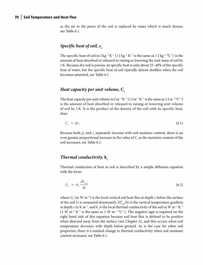
70 Soil Temperature and Heat Flux
as the air in the pores of the soil is replaced by water which is much denser,
see Table 6.1.
Specific heat of soil, cs
The specific heat of soil in J kg−1 K−1 (1 J kg−1 K−1 is the same as 1 J kg−1 °C−1) is the
amount of heat absorbed or released in raising or lowering the unit mass of soil by
1 K. Because dry soil is porous, its specific heat is only about 25–40% of the specific
heat of water, but the specific heat of soil typically almost doubles when the soil
becomes saturated, see Table 6.1.
Heat capacity per unit volume, Cs
The heat capacity per unit volume in J m−3 K−1 (1 J m−3 K−1 is the same as 1 J m−3 °C−1)
is the amount of heat absorbed or released in raising or lowering unit volume
of soil by 1 K. It is the product of the density of the soil with its specific heat,
thus:
s s sC c= r
(6.1)
Because both rs and c
s separately increase with soil moisture content, there is an
even greater proportional increase in the value of Cs as the moisture content of the
soil increases, see Table 6.1.
Thermal conductivity, ks
Thermal conduction of heat in soil is described by a simple diffusion equation
with the form:
soil
z s
TG k
z= −
∂∂
(6.2)
where Gz (in W m−2) is the local vertical soil heat flux at depth z below the surface
of the soil (z is measured downward), ∂Tsoil
/∂z is the vertical temperature gradient
at depth z in K m−1, and ks is the local thermal conductivity of the soil in W m−1 K−1
(1 W m−1 K−1 is the same as 1 W m−1 °C−1). The negative sign is required on the
right hand side of this equation because soil heat flux is defined to be positive
when directed away from the surface (see Chapter 4), and this occurs when soil
temperature decreases with depth below ground. As is the case for other soil
properties, there is a marked change in thermal conductivity when soil moisture
content increases, see Table 6.1.
Shuttleworth_c06.indd 70Shuttleworth_c06.indd 70 11/3/2011 6:32:12 PM11/3/2011 6:32:12 PM
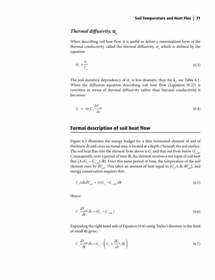
Soil Temperature and Heat Flux 71
Thermal diffusivity, as
When describing soil heat flow, it is useful to define a renormalized form of the
thermal conductivity called the thermal diffusivity, as, which is defined by the
equation:
ss
s
kC
=a
(6.3)
The soil moisture dependency of as, is less dramatic than for k
s, see Table 6.1.
When the diffusion equation describing soil heat flow (Equation (6.2)) is
rewritten in terms of thermal diffusivity rather than thermal conductivity it
becomes:
soilz s s
TG Cz
∂= −
∂a
(6.4)
Formal description of soil heat flow
Figure 6.3 illustrates the energy budget for a thin horizontal element of soil of
thickness dz and cross sectional area A located at a depth z beneath the soil surface.
The soil heat flux into the element from above is Gz and that out from below G
z+dz.
Consequently, over a period of time dt, the element receives a net input of soil heat
flux [A.(Gz − G
z+dz).dt]. Over this same period of time, the temperature of the soil
element rises by dTsoil
. This takes an amount of heat equal to [Cs.A.dz.dT
soil], and
energy conservation requires that:
( )s soil z z zC A z T A G G t+= − dd d d
(6.5)
Hence:
( )soils z z zTC z G Gt += − d
dd
d (6.6)
Expanding the right hand side of Equation (6.6) using Taylor’s theorem in the limit
of small dz gives:
.soil zs z zT GC z G G zt z
⎛ ⎞= − +⎜ ⎟⎝ ⎠d
d dd
∂∂
(6.7)
Shuttleworth_c06.indd 71Shuttleworth_c06.indd 71 11/3/2011 6:32:14 PM11/3/2011 6:32:14 PM

72 Soil Temperature and Heat Flux
Hence:
1soil z
s
T Gt C z
= −∂ ∂
∂ ∂
(6.8)
Substituting G from Equation (6.4) into this last equation gives:
1soil soils s
s
T TCt C z z
⎡ ⎤= ⎢ ⎥⎣ ⎦a
∂ ∂∂∂ ∂ ∂
(6.9)
In the particular case of heat flow in homogeneous soil for which both Cs and a
s
are constant with depth below ground, Equation (6.9) simplifies to:
2
2
soil soils
T Tt z
= a∂ ∂
∂ ∂ (6.10)
Thermal waves in homogeneous soil
Equation (6.9) can be solved numerically to provide a general description of the
evolution of soil temperature and therefore (from Equation (6.4)) soil heat flux in
response to a prescribed time series of soil surface temperature when the depth
dependency of Cs and a
s is defined. However, much can be learned about the
mechanics of soil heat flow by investigating the analytic solution of Equation (6.10)
which applies for homogeneous soil. It is also instructive to consider the case of
a simple sinusoidal variation in soil surface temperature, ,0tsoilT , described by the
expression:
,0 0( )
sin 2tsoil m a
t tT T TP−⎡ ⎤= + ⎢ ⎥⎣ ⎦
p
(6.11)
where Tm
is the mean temperature of the soil surface, Ta is the amplitude of the
sinusoidal variation in soil surface temperature, t is time in seconds, and P and t0
Soil surface
Area = A
Temperature = Tsoil
Air
Soil
z+δz z Gz
Gz+dz
Figure 6.3 Energy budget
for a thin horizontal element
of soil of thickness бz, cross
sectional area A, and
temperature Tsoil
located at a
depth z beneath the soil
surface, with soil heat flux Gz
entering from above and Gz+бz
leaving from below.
Shuttleworth_c06.indd 72Shuttleworth_c06.indd 72 11/3/2011 6:32:19 PM11/3/2011 6:32:19 PM
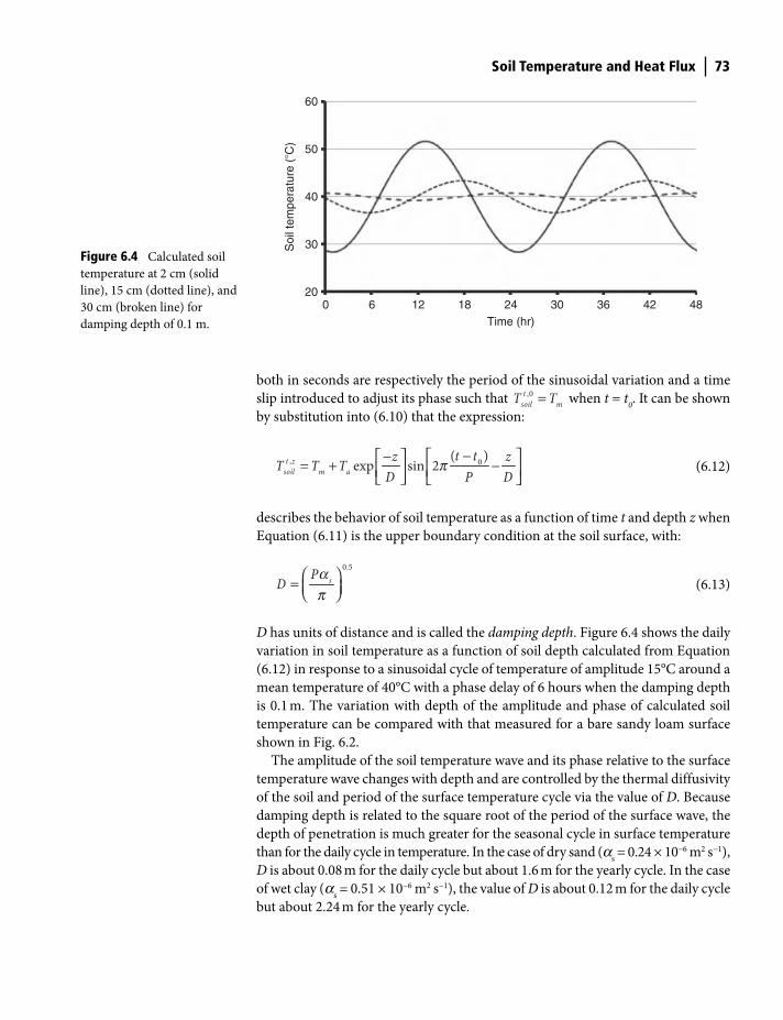
Soil Temperature and Heat Flux 73
both in seconds are respectively the period of the sinusoidal variation and a time
slip introduced to adjust its phase such that ,0tsoil mT T= when t = t
0. It can be shown
by substitution into (6.10) that the expression:
, 0( )
exp sin 2t zsoil m a
t tz zT T TD P D
−− ⎡ ⎤⎡ ⎤= + −⎢ ⎥⎢ ⎥⎣ ⎦ ⎣ ⎦p
(6.12)
describes the behavior of soil temperature as a function of time t and depth z when
Equation (6.11) is the upper boundary condition at the soil surface, with:
0.5
sPD ⎛ ⎞= ⎜ ⎟⎝ ⎠ap
(6.13)
D has units of distance and is called the damping depth. Figure 6.4 shows the daily
variation in soil temperature as a function of soil depth calculated from Equation
(6.12) in response to a sinusoidal cycle of temperature of amplitude 15°C around a
mean temperature of 40°C with a phase delay of 6 hours when the damping depth
is 0.1 m. The variation with depth of the amplitude and phase of calculated soil
temperature can be compared with that measured for a bare sandy loam surface
shown in Fig. 6.2.
The amplitude of the soil temperature wave and its phase relative to the surface
temperature wave changes with depth and are controlled by the thermal diffusivity
of the soil and period of the surface temperature cycle via the value of D. Because
damping depth is related to the square root of the period of the surface wave, the
depth of penetration is much greater for the seasonal cycle in surface temperature
than for the daily cycle in temperature. In the case of dry sand (as = 0.24 × 10⁻⁶ m2 s−1),
D is about 0.08 m for the daily cycle but about 1.6 m for the yearly cycle. In the case
of wet clay (as = 0.51 × 10⁻⁶ m2 s−1), the value of D is about 0.12 m for the daily cycle
but about 2.24 m for the yearly cycle.
18 24Time (hr)
30 36 42 48126020
30
40
50
60
Soi
l tem
pera
ture
(�C
)
Figure 6.4 Calculated soil
temperature at 2 cm (solid
line), 15 cm (dotted line), and
30 cm (broken line) for
damping depth of 0.1 m.
Shuttleworth_c06.indd 73Shuttleworth_c06.indd 73 11/3/2011 6:32:24 PM11/3/2011 6:32:24 PM
74 Soil Temperature and Heat Flux
The soil heat flux can be calculated at any depth in the soil using Equation (6.2)
or (6.4). However, it is the soil heat flux into the soil surface that is most often
required for use in calculating the energy budget of a sample volume lying between
ground level and a reference level in the atmosphere above. By differentiating
Equation (6.12) and substituting z = 0, it can be shown that for a homogeneous soil
and assuming the simple sinusoidal variation in surface temperature in Equation
(6.11), the surface soil heat flux is given by:
00
2 ( ) 2sin 2
8a s
zT k t tGD P=
−⎡ ⎤= +⎢ ⎥⎣ ⎦pp
(6.14)
Comparing Equation (6.14) with Equation (6.11) illustrates a general feature of
the relationship between soil heat flux and soil surface temperature. Specifically,
the sinusoidal wave in soil heat flux is advanced by one eighth of a cycle with
respect to the wave in surface temperature. This means that the peak soil heat
flow is approximately 3 hours earlier than the peak soil surface temperature
for the daily cycle, and the peak in soil heat flow is 1.5 months earlier than the
peak soil surface temperature for the yearly cycle. Physically this is because
there is most conduction of heat into the soil when the soil surface temperature
is rising rapidly in the morning for the daily cycle and in spring for the yearly
cycle, and most conduction of heat out of the soil when the soil surface
temperature is falling quickly in the evening for the daily cycle and in autumn
for the yearly cycle.
Equation (6.14) also shows that the magnitude of the wave in surface soil heat
flux is inversely proportional to the damping depth and therefore inversely
proportional to the square root of the period of the surface temperature wave,
see Equation (6.13). This means the amplitude of the soil heat flux wave associated
with the yearly cycle is (365)0.5 times less (i.e., about 19 times less) than the
amplitude of the daily cycle. The yearly cycle in soil heat flux is therefore about 20
times less than the daily wave but penetrates about 20 times deeper.
In fact the value of damping depth determines many interesting features of soil
heat flow as follows.
● The amplitude of temperature wave falls to e−1 (~0.37) of its surface value at
depth D
● The velocity with which temperature maximum and minimum appear to
propagate downward through the soil is given by (2πD/P)
● The temperature wave is π radians (180°) out of phase with the surface wave
at depth (πD)
● From Equation (6.14), the maximum surface heat flux is (√2.Ta.k
s)/D
which is the heat flow that would be maintained through a thickness
(√2.D) of soil if one side were maintained at (Tm
+Ta) and the other at
(Tm
–Ta). For this reason (√2.D) has been called the effective depth of soil
heat flow
Shuttleworth_c06.indd 74Shuttleworth_c06.indd 74 11/3/2011 6:32:27 PM11/3/2011 6:32:27 PM
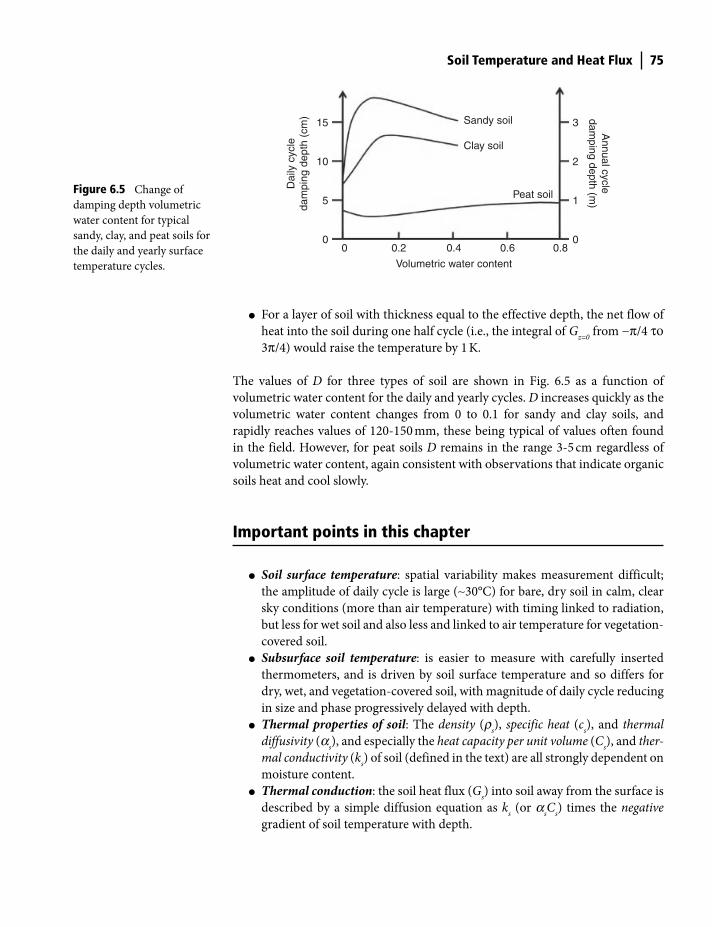
Soil Temperature and Heat Flux 75
● For a layer of soil with thickness equal to the effective depth, the net flow of
heat into the soil during one half cycle (i.e., the integral of Gz=0
from −π/4 το
3π/4) would raise the temperature by 1 K.
The values of D for three types of soil are shown in Fig. 6.5 as a function of
volumetric water content for the daily and yearly cycles. D increases quickly as the
volumetric water content changes from 0 to 0.1 for sandy and clay soils, and
rapidly reaches values of 120-150 mm, these being typical of values often found
in the field. However, for peat soils D remains in the range 3-5 cm regardless of
volumetric water content, again consistent with observations that indicate organic
soils heat and cool slowly.
Important points in this chapter
● Soil surface temperature: spatial variability makes measurement difficult;
the amplitude of daily cycle is large (∼30°C) for bare, dry soil in calm, clear
sky conditions (more than air temperature) with timing linked to radiation,
but less for wet soil and also less and linked to air temperature for vegetation-
covered soil.
● Subsurface soil temperature: is easier to measure with carefully inserted
thermometers, and is driven by soil surface temperature and so differs for
dry, wet, and vegetation-covered soil, with magnitude of daily cycle reducing
in size and phase progressively delayed with depth.
● Thermal properties of soil: The density (rs), specific heat (c
s), and thermal
diffusivity (as), and especially the heat capacity per unit volume (C
s), and ther-
mal conductivity (ks) of soil (defined in the text) are all strongly dependent on
moisture content.
● Thermal conduction: the soil heat flux (Gs) into soil away from the surface is
described by a simple diffusion equation as ks (or a
sC
s) times the negative
gradient of soil temperature with depth.
0 0.2 0.4
Volumetric water content
0.6 0.80
1
2
3
Annual cycle
damping depth (m
)
Dai
ly c
ycle
dam
ping
dep
th (
cm)
15
10
5
0
Clay soil
Sandy soil
Peat soilFigure 6.5 Change of
damping depth volumetric
water content for typical
sandy, clay, and peat soils for
the daily and yearly surface
temperature cycles.
Shuttleworth_c06.indd 75Shuttleworth_c06.indd 75 11/3/2011 6:32:28 PM11/3/2011 6:32:28 PM
76 Soil Temperature and Heat Flux
● Soil heat flow equation: the rate of change of soil temperature at depth is
given by the divergence of the equation describing thermal conduction, and
for homogeneous soil this becomes the product of the thermal diffusivity
with the second partial derivative of the soil temperature with depth.
● Thermal wave in soil temperature: assuming a sinusoidal daily cycle in soil
surface temperature and homogeneous soil, the thermal wave in the soil is
sinusoidal and relative to the surface wave has an amplitude less by a factor
(z/D) and phase (in radians) delayed by (z/D), where D (= √(Pas/π) is the
damping depth and P is the period of the wave in seconds.
● Damping depth: D is 0.08 m and 0.12 m for the daily soil surface temperature
cycle, and 1.6 m and 2.24 m for the yearly cycle for dry sandy soil and wet
clay, respectively.
● Surface soil heat flux: is advanced by one eighth of a cycle with respect to
sinusoidal variations in soil surface temperature, i.e., by 3 hours for the daily
cycle and 1.5 months for the yearly cycle.
References
Deacon, E.L. (1969) Physical processes near the surface of the Earth. In: World Survey of
Climatology, Vol. 1, General Climatology (ed. H.E. Landsberg). pp. 39–104. Elsevier,
Amsterdam.
Monteith, J.L. & Unsworth, M.H. (1990) Principles of Environmental Physics. Edward
Arnold, London.
Shuttleworth_c06.indd 76Shuttleworth_c06.indd 76 11/3/2011 6:32:28 PM11/3/2011 6:32:28 PM

Introduction
This chapter provides an overview of some of the most commonly used methods
by means of which important terms in the surface energy budget are measured.
Most measurement methods provide an estimate of the average rate of flow of
energy into or out of the Earth’s surface over a specified period. However, latent
heat flux is also frequently measured in the form of the net evaporative water loss
from sample areas of the terrestrial surface.
Measuring solar radiation
The most common early approach used to derive surface solar radiation was to
estimate how much of the calculable solar energy entering the top of the atmosphere
was absorbed before it reached the ground. This required estimates or
measurements of cloud cover. Subsequently, instruments were devised which
measured the incident solar energy from the warming it induced when incident
on a near blackbody surface or from the number of electrons it mobilized in a
semiconductor.
Daily estimates of cloud cover
Estimates of cloud cover are made with the human eye by trained observers at
meteorological stations looking upward at the sky overhead. When estimates are
made in this way, they are usually expressed either in oktas (eighths of the sky) or
in tenths and given to the closest whole number value. A value of 0 refers to clear
7 Measuring Surface Heat Fluxes
Terrestrial Hydrometeorology, First Edition. W. James Shuttleworth.
© 2012 John Wiley & Sons, Ltd. Published 2012 by John Wiley & Sons, Ltd.
Shuttleworth_c07.indd 77Shuttleworth_c07.indd 77 11/3/2011 6:31:01 PM11/3/2011 6:31:01 PM
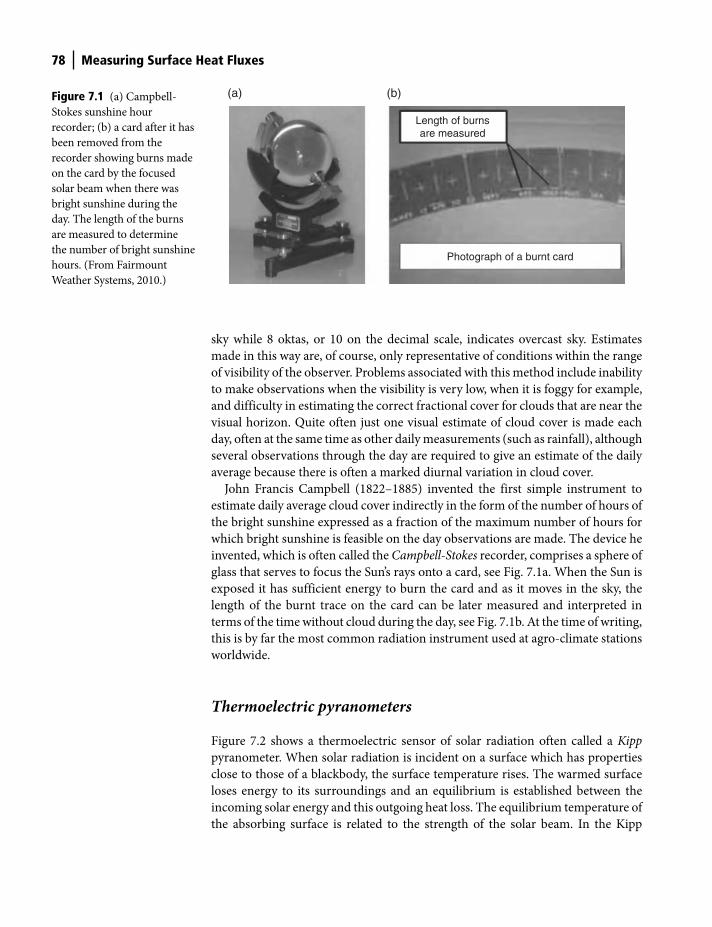
78 Measuring Surface Heat Fluxes
sky while 8 oktas, or 10 on the decimal scale, indicates overcast sky. Estimates
made in this way are, of course, only representative of conditions within the range
of visibility of the observer. Problems associated with this method include inability
to make observations when the visibility is very low, when it is foggy for example,
and difficulty in estimating the correct fractional cover for clouds that are near the
visual horizon. Quite often just one visual estimate of cloud cover is made each
day, often at the same time as other daily measurements (such as rainfall), although
several observations through the day are required to give an estimate of the daily
average because there is often a marked diurnal variation in cloud cover.
John Francis Campbell (1822–1885) invented the first simple instrument to
estimate daily average cloud cover indirectly in the form of the number of hours of
the bright sunshine expressed as a fraction of the maximum number of hours for
which bright sunshine is feasible on the day observations are made. The device he
invented, which is often called the Campbell-Stokes recorder, comprises a sphere of
glass that serves to focus the Sun’s rays onto a card, see Fig. 7.1a. When the Sun is
exposed it has sufficient energy to burn the card and as it moves in the sky, the
length of the burnt trace on the card can be later measured and interpreted in
terms of the time without cloud during the day, see Fig. 7.1b. At the time of writing,
this is by far the most common radiation instrument used at agro-climate stations
worldwide.
Thermoelectric pyranometers
Figure 7.2 shows a thermoelectric sensor of solar radiation often called a Kipp
pyranometer. When solar radiation is incident on a surface which has properties
close to those of a blackbody, the surface temperature rises. The warmed surface
loses energy to its surroundings and an equilibrium is established between the
incoming solar energy and this outgoing heat loss. The equilibrium temperature of
the absorbing surface is related to the strength of the solar beam. In the Kipp
Length of burnsare measured
(a) (b)
Photograph of a burnt card
Figure 7.1 (a) Campbell-
Stokes sunshine hour
recorder; (b) a card after it has
been removed from the
recorder showing burns made
on the card by the focused
solar beam when there was
bright sunshine during the
day. The length of the burns
are measured to determine
the number of bright sunshine
hours. (From Fairmount
Weather Systems, 2010.)
Shuttleworth_c07.indd 78Shuttleworth_c07.indd 78 11/3/2011 6:31:02 PM11/3/2011 6:31:02 PM
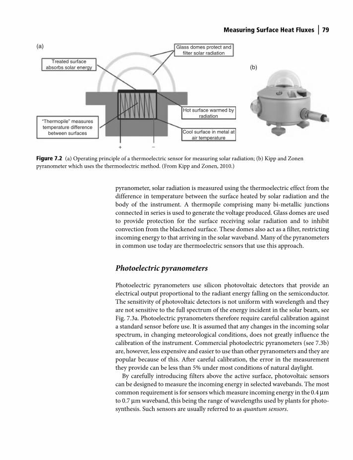
Measuring Surface Heat Fluxes 79
pyranometer, solar radiation is measured using the thermoelectric effect from the
difference in temperature between the surface heated by solar radiation and the
body of the instrument. A thermopile comprising many bi-metallic junctions
connected in series is used to generate the voltage produced. Glass domes are used
to provide protection for the surface receiving solar radiation and to inhibit
convection from the blackened surface. These domes also act as a filter, restricting
incoming energy to that arriving in the solar waveband. Many of the pyranometers
in common use today are thermoelectric sensors that use this approach.
Photoelectric pyranometers
Photoelectric pyranometers use silicon photovoltaic detectors that provide an
electrical output proportional to the radiant energy falling on the semiconductor.
The sensitivity of photovoltaic detectors is not uniform with wavelength and they
are not sensitive to the full spectrum of the energy incident in the solar beam, see
Fig. 7.3a. Photoelectric pyranometers therefore require careful calibration against
a standard sensor before use. It is assumed that any changes in the incoming solar
spectrum, in changing meteorological conditions, does not greatly influence the
calibration of the instrument. Commercial photoelectric pyranometers (see 7.3b)
are, however, less expensive and easier to use than other pyranometers and they are
popular because of this. After careful calibration, the error in the measurement
they provide can be less than 5% under most conditions of natural daylight.
By carefully introducing filters above the active surface, photovoltaic sensors
can be designed to measure the incoming energy in selected wavebands. The most
common requirement is for sensors which measure incoming energy in the 0.4 μm
to 0.7 μm waveband, this being the range of wavelengths used by plants for photo-
synthesis. Such sensors are usually referred to as quantum sensors.
Treated surfaceabsorbs solar energy
Glass domes protect andfilter solar radiation
(a)
(b)
Hot surface warmed byradiation
Cool surface in metal atair temperature
“Thermopile” measurestemperature difference
between surfaces
+ −
Figure 7.2 (a) Operating principle of a thermoelectric sensor for measuring solar radiation; (b) Kipp and Zonen
pyranometer which uses the thermoelectric method. (From Kipp and Zonen, 2010.)
Shuttleworth_c07.indd 79Shuttleworth_c07.indd 79 11/3/2011 6:31:02 PM11/3/2011 6:31:02 PM
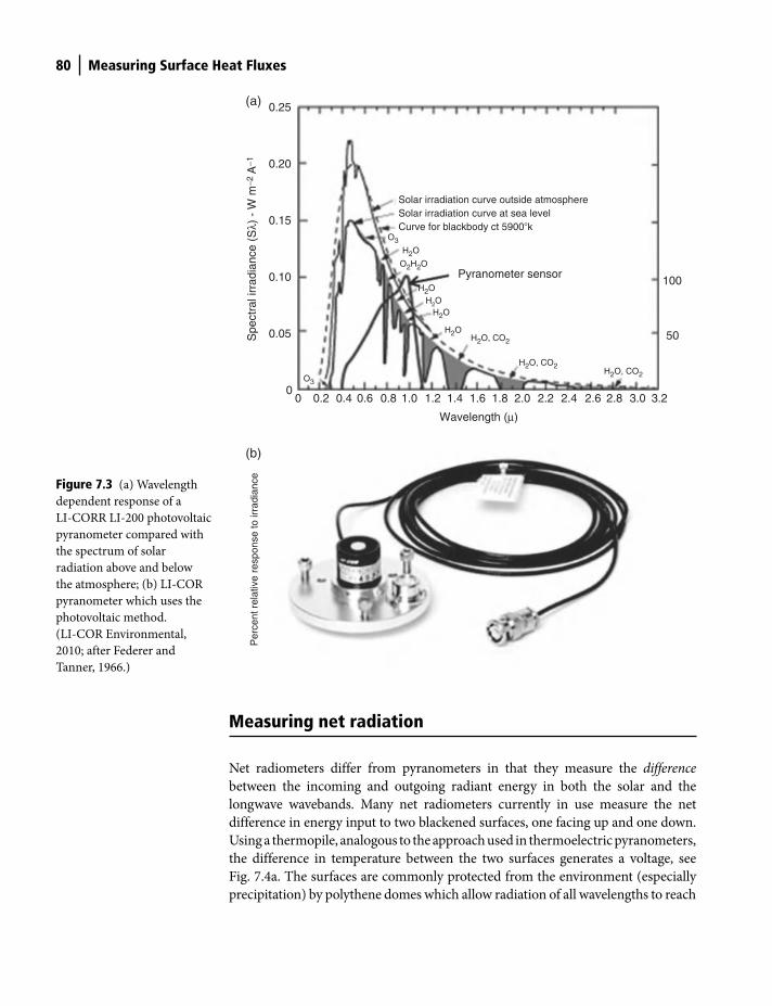
80 Measuring Surface Heat Fluxes
Measuring net radiation
Net radiometers differ from pyranometers in that they measure the difference
between the incoming and outgoing radiant energy in both the solar and the
longwave wavebands. Many net radiometers currently in use measure the net
difference in energy input to two blackened surfaces, one facing up and one down.
Using a thermopile, analogous to the approach used in thermoelectric pyranometers,
the difference in temperature between the two surfaces generates a voltage, see
Fig. 7.4a. The surfaces are commonly protected from the environment (especially
precipitation) by polythene domes which allow radiation of all wavelengths to reach
0.05
0.10
0.15
0.20
0.25
00 0.2 0.4 0.6 0.8 1.0 1.2 1.4 1.6
Solar irradiation curve outside atmosphereSolar irradiation curve at sea levelCurve for blackbody ct 5900�k
O3
O3
O2H2O
H2O
H2OH2O
H2O
H2OH2O, CO2
H2O, CO2H2O, CO2
50
100
Wavelength (μ)
1.8 2.0
Pyranometer sensor
(a)
(b)
2.2 2.4 2.6 2.8 3.0 3.2
Per
cent
rel
ativ
e re
spon
se to
irra
dian
ceS
pect
ral i
rrad
ianc
e (S
λ) -
W m
−2 A
−1
Figure 7.3 (a) Wavelength
dependent response of a
LI-CORR LI-200 photovoltaic
pyranometer compared with
the spectrum of solar
radiation above and below
the atmosphere; (b) LI-COR
pyranometer which uses the
photovoltaic method.
(LI-COR Environmental,
2010; after Federer and
Tanner, 1966.)
Shuttleworth_c07.indd 80Shuttleworth_c07.indd 80 11/3/2011 6:31:03 PM11/3/2011 6:31:03 PM
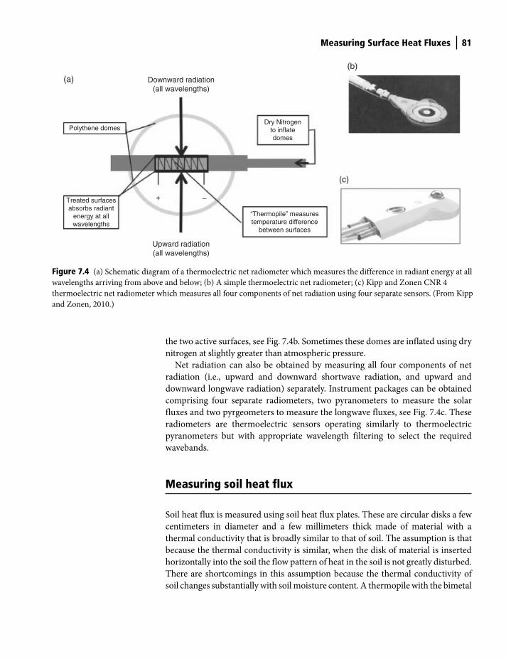
Measuring Surface Heat Fluxes 81
the two active surfaces, see Fig. 7.4b. Sometimes these domes are inflated using dry
nitrogen at slightly greater than atmospheric pressure.
Net radiation can also be obtained by measuring all four components of net
radiation (i.e., upward and downward shortwave radiation, and upward and
downward longwave radiation) separately. Instrument packages can be obtained
comprising four separate radiometers, two pyranometers to measure the solar
fluxes and two pyrgeometers to measure the longwave fluxes, see Fig. 7.4c. These
radiometers are thermoelectric sensors operating similarly to thermoelectric
pyranometers but with appropriate wavelength filtering to select the required
wavebands.
Measuring soil heat flux
Soil heat flux is measured using soil heat flux plates. These are circular disks a few
centimeters in diameter and a few millimeters thick made of material with a
thermal conductivity that is broadly similar to that of soil. The assumption is that
because the thermal conductivity is similar, when the disk of material is inserted
horizontally into the soil the flow pattern of heat in the soil is not greatly disturbed.
There are shortcomings in this assumption because the thermal conductivity of
soil changes substantially with soil moisture content. A thermopile with the bimetal
(b)
(c)
Polythene domes
Treated surfacesabsorbs radiant
energy at allwavelengths
Dry Nitrogento inflatedomes
“Thermopile” measurestemperature difference
between surfaces
Upward radiation(all wavelengths)
Downward radiation(all wavelengths)
(a)
+ −
Figure 7.4 (a) Schematic diagram of a thermoelectric net radiometer which measures the difference in radiant energy at all
wavelengths arriving from above and below; (b) A simple thermoelectric net radiometer; (c) Kipp and Zonen CNR 4
thermoelectric net radiometer which measures all four components of net radiation using four separate sensors. (From Kipp
and Zonen, 2010.)
Shuttleworth_c07.indd 81Shuttleworth_c07.indd 81 11/3/2011 6:31:03 PM11/3/2011 6:31:03 PM

82 Measuring Surface Heat Fluxes
junctions alternately near the top and bottom of the soil heat plate measures the
temperature difference across the soil heat flux plate. Because the thermal
conductivity and thickness of the soil heat flux plate are known, the heat flow per
unit area through the plate can be calculated and this is assumed to be the same as
that which would be flowing through the volume of soil that the plate replaces.
Soil heat flux plates cannot realistically be used on the surface of the soil so they
are normally installed at some depth (typically 5 cm) below the soil surface, see
Fig. 7.5. Because the damping depth of heat flow in soils is typically on the order
of 5–15 cm, this means the soil heat flux measured by the plate is not a good
estimate of the surface soil heat flux. Therefore, an attempt is made to estimate the
loss or gain of heat in the layer of soil between the plate and the surface. To do this
at least one and usually more thermometers are inserted into the soil to measure
the rate of change of soil temperature between the soil flux plate and the surface.
Often a pit with a vertical edge is dug and these thermometers and the soil heat
flux plate are inserted sideways into the soil through the edge of the pit to minimize
soil disturbance.
If the heat capacity per unit volume of the soil, Cs, is known, the corrected soil heat
flux at the surface is estimated from the soil heat flux measure by the plate using:
= =
δ= +
δ0
soilz z d s
TG G C
t (7.1)
where Gz=0
and Gz=d
are respectively the soil heat fluxes at the surface and at depth
d at which the soil heat flux plate is inserted, and dTsoil
is the average change in the
temperature of the soil layer above the plate over the period dt for which estima-
tion is required.
Measuring latent and sensible heat
There are two general ways in which the fluxes of latent and sensible heat are
measured. One is to determine one or both of these energy fluxes by making
meteorological measurements in the turbulent air just above the surface through
Soil heatflux plate
Soil surface
Soil
Air
Soilthermometers
Gz =0
Gz =0
~5 cm
Figure 7.5 Arrangement of a
soil heat flux plate and soil
thermometers when used to
estimate the heat flux at the
soil surface.
Shuttleworth_c07.indd 82Shuttleworth_c07.indd 82 11/3/2011 6:31:04 PM11/3/2011 6:31:04 PM
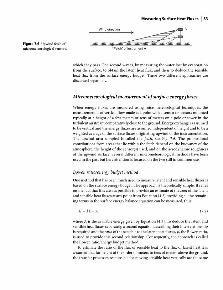
Measuring Surface Heat Fluxes 83
which they pass. The second way is, by measuring the water lost by evaporation
from the surface, to obtain the latent heat flux, and then to deduce the sensible
heat flux from the surface energy budget. These two different approaches are
discussed separately.
Micrometeorological measurement of surface energy fluxes
When energy fluxes are measured using micrometeorological techniques, the
measurement is of vertical flow made at a point with a sensor or sensors mounted
typically at a height of a few meters or tens of meters on a pole or tower in the
turbulent airstream comparatively close to the ground. Energy exchange is assumed
to be vertical and the energy fluxes are assumed independent of height and to be a
weighted average of the surface fluxes originating upwind of the instrumentation.
The upwind area sampled is called the fetch, see Fig. 7.6. The proportional
contributions from areas that lie within the fetch depend on the buoyancy of the
atmosphere, the height of the sensor(s) used, and on the aerodynamic roughness
of the upwind surface. Several different micrometeorological methods have been
used in the past but here attention is focused on the two still in common use.
Bowen ratio/energy budget method
One method that has been much used to measure latent and sensible heat fluxes is
based on the surface energy budget. The approach is theoretically simple. It relies
on the fact that it is always possible to provide an estimate of the sum of the latent
and sensible heat fluxes at any point from Equation (4.2) providing all the remain-
ing terms in the surface energy balance equation can be measured, thus:
+ =H E Al (7.2)
where A is the available energy given by Equation (4.3). To deduce the latent and
sensible heat fluxes separately, a second equation describing their interrelationship
is required and the ratio of the sensible to the latent heat fluxes, b, the Bowen ratio,
is used to provide this second relationship. Consequently, the approach is called
the Bowen ratio/energy budget method.
To estimate the ratio of the flux of sensible heat to the flux of latent heat it is
assumed that for height of the order of meters to tens of meters above the ground,
the transfer processes responsible for moving sensible heat vertically are the same
Wind direction
“Fetch” of instrument A
A
Figure 7.6 Upwind fetch of
micrometeorological sensors.
Shuttleworth_c07.indd 83Shuttleworth_c07.indd 83 11/3/2011 6:31:05 PM11/3/2011 6:31:05 PM

84 Measuring Surface Heat Fluxes
as those that move latent heat vertically, and that these are equally effective in each
case. Recognizing the need to express temperatures in terms of virtual potential
temperature when describing flow in a hydrostatic atmosphere (see Chapter 3), the
rate of vertical sensible heat flow between two levels is assumed to be proportional
to the difference in atmospheric heat content at these two levels, i.e., proportional
to the difference in (rac
pq
v). Similarly, the rate of water vapor flow between the
same two levels is assumed to be proportional to the difference in humidity content
between the two levels, i.e., proportional to the difference (raq), and latent heat
flow is then proportional to this difference multiplied by λ. Consider two levels
where the potential temperatures are qv1 and q
v2, respectively, and the specific
humidities are q1 and q2, respectively. If the processes for the transfer of heat and
water vapor are the same between these levels, then β is given by:
⎡ ⎤−⎣ ⎦=⎡ ⎤−⎣ ⎦
2 1
2 1
( ) ( )
( ) ( )
a p v a p v
a a
c c
q q
r q r qb
r l r l (7.3)
Substituting for q using Equation (2.9), this equation can be rewritten as:
Δ= =
ΔvH
E eq
b gl
(7.4)
where Δθv and Δe are the differences in virtual potential temperature and vapor
pressure between levels 1 and 2, respectively, and γ is the psychrometric constant
defined by Equation (2.25). Because the sum and the ratio of the sensible heat and
latent heat fluxes are known, individual values of these two fluxes can be calcu-
lated by combining Equations (7.2) and (7.4) to give:
( )=+1
AElb
(7.5)
and:
= −H A El (7.6)
Measuring the difference in air temperature and humidity between two heights
required to calculate the Bowen ratio from Equation (7.4) can be difficult if these
differences are comparable in size with systematic errors in the instruments used.
But field systems have been designed to minimize the effect of sensor errors; one
approach (Fig. 7.7) is to regularly interchange pairs of temperature and humidity
sensors between the two levels. In practice, measuring the difference in humidity
is usually more difficult than measuring the difference in temperature and an
effective way to minimize the effect of humidity measurement errors is to duct air
alternately from the two levels to a common humidity sensor (Fig. 7.8). The effect
of any instrumental offset error then cancels out in the measured difference.
Shuttleworth_c07.indd 84Shuttleworth_c07.indd 84 11/3/2011 6:31:06 PM11/3/2011 6:31:06 PM
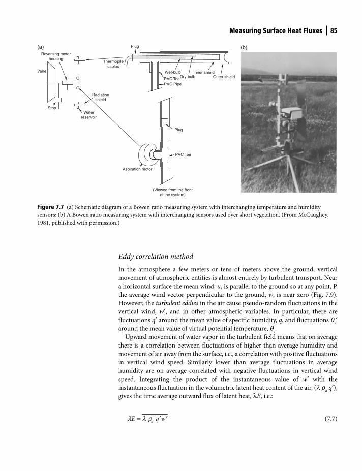
Measuring Surface Heat Fluxes 85
Eddy correlation method
In the atmosphere a few meters or tens of meters above the ground, vertical
movement of atmospheric entities is almost entirely by turbulent transport. Near
a horizontal surface the mean wind, u, is parallel to the ground so at any point, P,
the average wind vector perpendicular to the ground, w, is near zero (Fig. 7.9).
However, the turbulent eddies in the air cause pseudo-random fluctuations in the
vertical wind, w′, and in other atmospheric variables. In particular, there are
fluctuations q′ around the mean value of specific humidity, q, and fluctuations qv′
around the mean value of virtual potential temperature, qv.
Upward movement of water vapor in the turbulent field means that on average
there is a correlation between fluctuations of higher than average humidity and
movement of air away from the surface, i.e., a correlation with positive fluctuations
in vertical wind speed. Similarly lower than average fluctuations in average
humidity are on average correlated with negative fluctuations in vertical wind
speed. Integrating the product of the instantaneous value of w′ with the
instantaneous fluctuation in the volumetric latent heat content of the air, (l ra q′),
gives the time average outward flux of latent heat, λE, i.e.:
= ′ ′ aE q wl l r (7.7)
(b)Reversing motor
housing
Vane
StopWater
reservoir
Radiationshield
Thermopilecables
Plug(a)
Wet-bulb Inner shieldOuter shieldDry-bulb
Plug
PVC Tee
PVC Tee
Aspiration motor
(Viewed from the frontof the system)
PVC Pipe
Figure 7.7 (a) Schematic diagram of a Bowen ratio measuring system with interchanging temperature and humidity
sensors; (b) A Bowen ratio measuring system with interchanging sensors used over short vegetation. (From McCaughey,
1981, published with permission.)
Shuttleworth_c07.indd 85Shuttleworth_c07.indd 85 11/3/2011 6:31:10 PM11/3/2011 6:31:10 PM
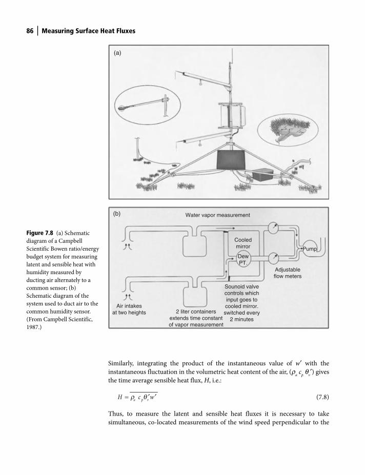
86 Measuring Surface Heat Fluxes
Similarly, integrating the product of the instantaneous value of w′ with the
instantaneous fluctuation in the volumetric heat content of the air, (ra c
p q
v′) gives
the time average sensible heat flux, H, i.e.:
a p vH c w= ′ ′r q (7.8)
Thus, to measure the latent and sensible heat fluxes it is necessary to take
simultaneous, co-located measurements of the wind speed perpendicular to the
Water vapor measurement
(a)
(b)
Cooledmirror
DewPT.
Pump
Adjustableflow meters
2 liter containersextends time constantof vapor measurement
Air intakesat two heights
Sounoid valvecontrols whichinput goes tocooled mirror.switched every
2 minutes
Figure 7.8 (a) Schematic
diagram of a Campbell
Scientific Bowen ratio/energy
budget system for measuring
latent and sensible heat with
humidity measured by
ducting air alternately to a
common sensor; (b)
Schematic diagram of the
system used to duct air to the
common humidity sensor.
(From Campbell Scientific,
1987.)
Shuttleworth_c07.indd 86Shuttleworth_c07.indd 86 11/3/2011 6:31:11 PM11/3/2011 6:31:11 PM
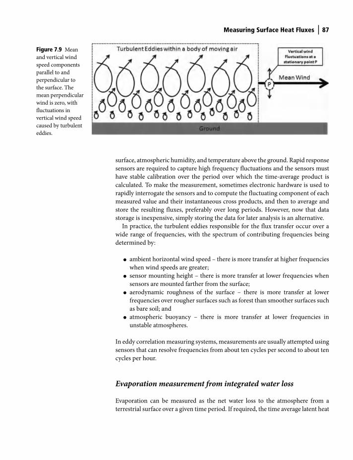
Measuring Surface Heat Fluxes 87
surface, atmospheric humidity, and temperature above the ground. Rapid response
sensors are required to capture high frequency fluctuations and the sensors must
have stable calibration over the period over which the time-average product is
calculated. To make the measurement, sometimes electronic hardware is used to
rapidly interrogate the sensors and to compute the fluctuating component of each
measured value and their instantaneous cross products, and then to average and
store the resulting fluxes, preferably over long periods. However, now that data
storage is inexpensive, simply storing the data for later analysis is an alternative.
In practice, the turbulent eddies responsible for the flux transfer occur over a
wide range of frequencies, with the spectrum of contributing frequencies being
determined by:
● ambient horizontal wind speed – there is more transfer at higher frequencies
when wind speeds are greater;
● sensor mounting height – there is more transfer at lower frequencies when
sensors are mounted farther from the surface;
● aerodynamic roughness of the surface – there is more transfer at lower
frequencies over rougher surfaces such as forest than smoother surfaces such
as bare soil; and
● atmospheric buoyancy – there is more transfer at lower frequencies in
unstable atmospheres.
In eddy correlation measuring systems, measurements are usually attempted using
sensors that can resolve frequencies from about ten cycles per second to about ten
cycles per hour.
Evaporation measurement from integrated water loss
Evaporation can be measured as the net water loss to the atmosphere from a
terrestrial surface over a given time period. If required, the time average latent heat
Figure 7.9 Mean
and vertical wind
speed components
parallel to and
perpendicular to
the surface. The
mean perpendicular
wind is zero, with
fluctuations in
vertical wind speed
caused by turbulent
eddies.
Shuttleworth_c07.indd 87Shuttleworth_c07.indd 87 11/3/2011 6:31:13 PM11/3/2011 6:31:13 PM
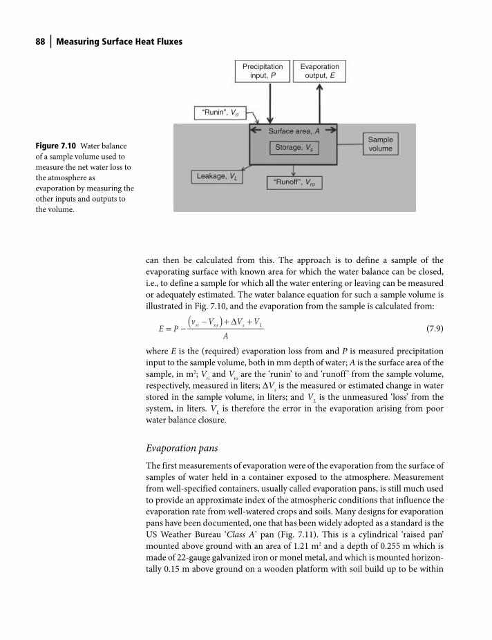
88 Measuring Surface Heat Fluxes
can then be calculated from this. The approach is to define a sample of the
evaporating surface with known area for which the water balance can be closed,
i.e., to define a sample for which all the water entering or leaving can be measured
or adequately estimated. The water balance equation for such a sample volume is
illustrated in Fig. 7.10, and the evaporation from the sample is calculated from:
( )− + Δ += − ri ro s Lv V V V
E PA
(7.9)
where E is the (required) evaporation loss from and P is measured precipitation
input to the sample volume, both in mm depth of water; A is the surface area of the
sample, in m2; Vri and V
ro are the ‘runin’ to and ‘runoff ’ from the sample volume,
respectively, measured in liters; ΔVs is the measured or estimated change in water
stored in the sample volume, in liters; and VL is the unmeasured ‘loss’ from the
system, in liters. VL is therefore the error in the evaporation arising from poor
water balance closure.
Evaporation pans
The first measurements of evaporation were of the evaporation from the surface of
samples of water held in a container exposed to the atmosphere. Measurement
from well-specified containers, usually called evaporation pans, is still much used
to provide an approximate index of the atmospheric conditions that influence the
evaporation rate from well-watered crops and soils. Many designs for evaporation
pans have been documented, one that has been widely adopted as a standard is the
US Weather Bureau ‘Class A’ pan (Fig. 7.11). This is a cylindrical ‘raised pan’
mounted above ground with an area of 1.21 m2 and a depth of 0.255 m which is
made of 22-gauge galvanized iron or monel metal, and which is mounted horizon-
tally 0.15 m above ground on a wooden platform with soil build up to be within
Precipitationinput, P
Evaporationoutput, E
“Runin”, Vri
“Runoff”, Vro
Surface area, A
Storage, VsSamplevolume
Leakage, VL
Figure 7.10 Water balance
of a sample volume used to
measure the net water loss to
the atmosphere as
evaporation by measuring the
other inputs and outputs to
the volume.
Shuttleworth_c07.indd 88Shuttleworth_c07.indd 88 11/3/2011 6:31:14 PM11/3/2011 6:31:14 PM
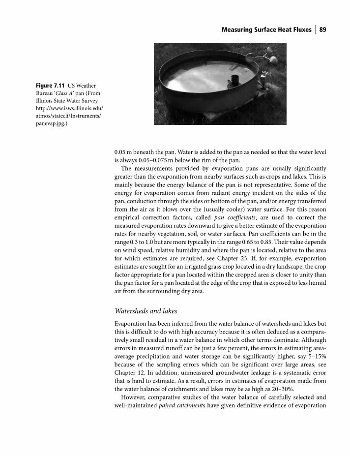
Measuring Surface Heat Fluxes 89
0.05 m beneath the pan. Water is added to the pan as needed so that the water level
is always 0.05–0.075 m below the rim of the pan.
The measurements provided by evaporation pans are usually significantly
greater than the evaporation from nearby surfaces such as crops and lakes. This is
mainly because the energy balance of the pan is not representative. Some of the
energy for evaporation comes from radiant energy incident on the sides of the
pan, conduction through the sides or bottom of the pan, and/or energy transferred
from the air as it blows over the (usually cooler) water surface. For this reason
empirical correction factors, called pan coefficients, are used to correct the
measured evaporation rates downward to give a better estimate of the evaporation
rates for nearby vegetation, soil, or water surfaces. Pan coefficients can be in the
range 0.3 to 1.0 but are more typically in the range 0.65 to 0.85. Their value depends
on wind speed, relative humidity and where the pan is located, relative to the area
for which estimates are required, see Chapter 23. If, for example, evaporation
estimates are sought for an irrigated grass crop located in a dry landscape, the crop
factor appropriate for a pan located within the cropped area is closer to unity than
the pan factor for a pan located at the edge of the crop that is exposed to less humid
air from the surrounding dry area.
Watersheds and lakes
Evaporation has been inferred from the water balance of watersheds and lakes but
this is difficult to do with high accuracy because it is often deduced as a compara-
tively small residual in a water balance in which other terms dominate. Although
errors in measured runoff can be just a few percent, the errors in estimating area-
average precipitation and water storage can be significantly higher, say 5–15%
because of the sampling errors which can be significant over large areas, see
Chapter 12. In addition, unmeasured groundwater leakage is a systematic error
that is hard to estimate. As a result, errors in estimates of evaporation made from
the water balance of catchments and lakes may be as high as 20–30%.
However, comparative studies of the water balance of carefully selected and
well-maintained paired catchments have given definitive evidence of evaporation
Figure 7.11 US Weather
Bureau ‘Class A’ pan (From
Illinois State Water Survey
http://www.isws.illinois.edu/
atmos/statecli/Instruments/
panevap.jpg.)
Shuttleworth_c07.indd 89Shuttleworth_c07.indd 89 11/3/2011 6:31:15 PM11/3/2011 6:31:15 PM
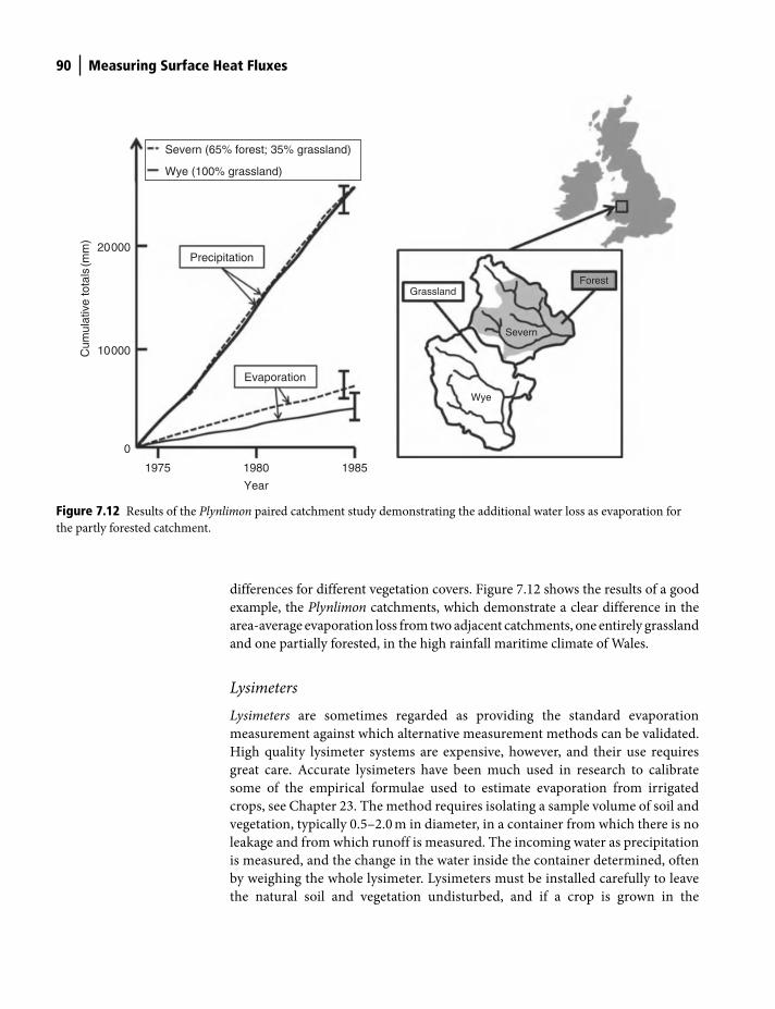
90 Measuring Surface Heat Fluxes
differences for different vegetation covers. Figure 7.12 shows the results of a good
example, the Plynlimon catchments, which demonstrate a clear difference in the
area-average evaporation loss from two adjacent catchments, one entirely grassland
and one partially forested, in the high rainfall maritime climate of Wales.
Lysimeters
Lysimeters are sometimes regarded as providing the standard evaporation
measurement against which alternative measurement methods can be validated.
High quality lysimeter systems are expensive, however, and their use requires
great care. Accurate lysimeters have been much used in research to calibrate
some of the empirical formulae used to estimate evaporation from irrigated
crops, see Chapter 23. The method requires isolating a sample volume of soil and
vegetation, typically 0.5–2.0 m in diameter, in a container from which there is no
leakage and from which runoff is measured. The incoming water as precipitation
is measured, and the change in the water inside the container determined, often
by weighing the whole lysimeter. Lysimeters must be installed carefully to leave
the natural soil and vegetation undisturbed, and if a crop is grown in the
GrasslandForest
Severn
Wye
1975 1980 1985
Year
Evaporation
Cum
ulat
ive
tota
ls(m
m)
Precipitation
Severn (65% forest; 35% grassland)
Wye (100% grassland)
20000
10000
0
Figure 7.12 Results of the Plynlimon paired catchment study demonstrating the additional water loss as evaporation for
the partly forested catchment.
Shuttleworth_c07.indd 90Shuttleworth_c07.indd 90 11/3/2011 6:31:15 PM11/3/2011 6:31:15 PM
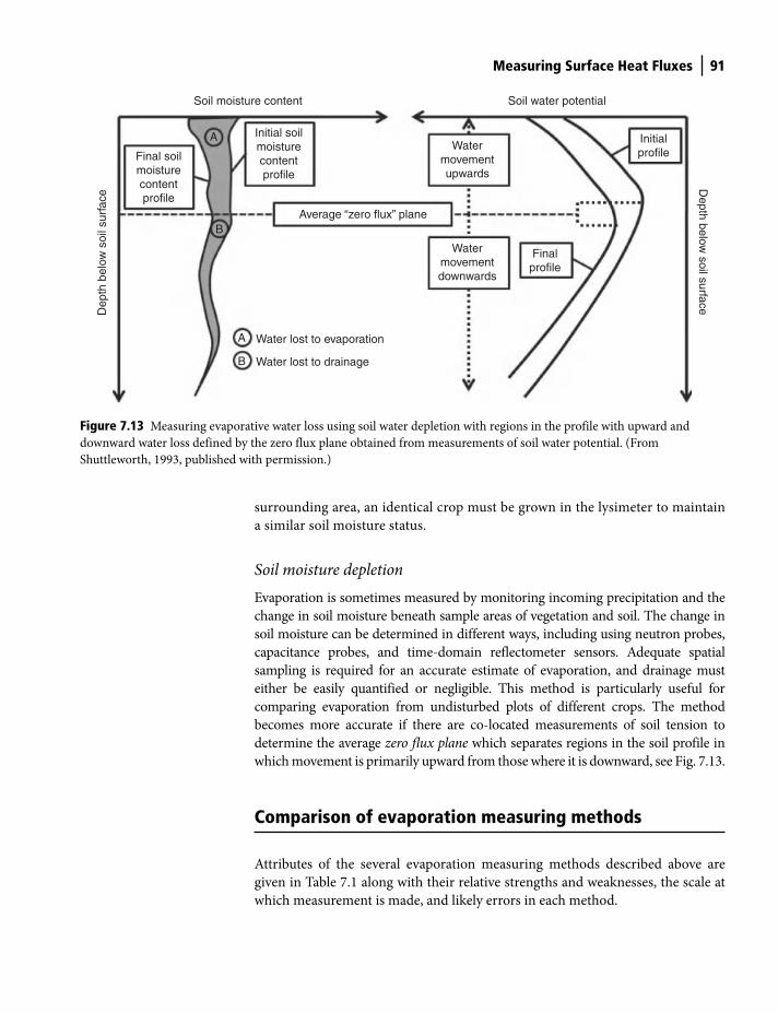
Measuring Surface Heat Fluxes 91
surrounding area, an identical crop must be grown in the lysimeter to maintain
a similar soil moisture status.
Soil moisture depletion
Evaporation is sometimes measured by monitoring incoming precipitation and the
change in soil moisture beneath sample areas of vegetation and soil. The change in
soil moisture can be determined in different ways, including using neutron probes,
capacitance probes, and time-domain reflectometer sensors. Adequate spatial
sampling is required for an accurate estimate of evaporation, and drainage must
either be easily quantified or negligible. This method is particularly useful for
comparing evaporation from undisturbed plots of different crops. The method
becomes more accurate if there are co-located measurements of soil tension to
determine the average zero flux plane which separates regions in the soil profile in
which movement is primarily upward from those where it is downward, see Fig. 7.13.
Comparison of evaporation measuring methods
Attributes of the several evaporation measuring methods described above are
given in Table 7.1 along with their relative strengths and weaknesses, the scale at
which measurement is made, and likely errors in each method.
Water lost to evaporation
Watermovementdownwards
Watermovementupwards
Finalprofile
Initial soilmoisturecontentprofile
Soil moisture content Soil water potential
Final soilmoisturecontentprofile
Average “zero flux” plane
Dep
th b
elow
soi
l sur
face
Depth below
soil surface
Initialprofile
Water lost to drainageB
B
A
A
Figure 7.13 Measuring evaporative water loss using soil water depletion with regions in the profile with upward and
downward water loss defined by the zero flux plane obtained from measurements of soil water potential. (From
Shuttleworth, 1993, published with permission.)
Shuttleworth_c07.indd 91Shuttleworth_c07.indd 91 11/3/2011 6:31:16 PM11/3/2011 6:31:16 PM

Tabl
e 7.
1 Su
mm
ary
of
attr
ibu
tes
of
dif
fere
nt
met
ho
d f
or
mea
suri
ng
evap
ora
tio
n a
lon
g w
ith
op
inio
ns
on
th
eir
rela
tive
str
engt
hs
and
wea
kn
esse
s, t
he
scal
e at
wh
ich
mea
sure
men
t is
mad
e, a
nd
lik
ely
erro
rs i
n e
ach
met
ho
d.
Mic
rom
eteo
rolo
gica
l m
etho
dsBr
ief
Des
crip
tion
Ass
umpt
ions
Stre
ngth
s an
d w
eakn
esse
sSc
ale
of
Mea
sure
men
tEr
ror
Bow
en R
atio
– E
nerg
y Bu
dget
Calc
ulat
e ev
apor
atio
n as
the
late
nt h
eat f
rom
the
surfa
ce
ener
gy b
udge
t usin
g th
e ra
tio o
f sen
sible
to la
tent
he
at (B
owen
ratio
) der
ived
fro
m th
e ra
tio b
etw
een
atm
osph
eric
tem
pera
ture
an
d hu
mid
ity g
radi
ents
m
easu
red
over
a fe
w m
eter
s ab
ove
the
vege
tatio
n.
Assu
mes
the
turb
ulen
t diff
usio
n co
effic
ient
for s
ensib
le h
eat a
nd
late
nt h
eat a
re th
e sa
me
in th
e lo
wer
atm
osph
ere
in a
ll co
nditi
ons
of a
tmos
pher
ic
stab
ility
, and
sam
ple
plot
sca
le
mea
sure
men
ts o
f ene
rgy
budg
et
com
pone
nts
(net
radi
atio
n, s
oil
heat
) are
repr
esen
tive
of
upw
ind
cond
ition
s.
Fairl
y w
ell e
stab
lishe
d m
etho
d w
hich
is
ava
ilabl
e as
rela
tivel
y in
expe
nsiv
e pr
oprie
tary
sys
tem
s th
at c
an b
e us
ed
for b
oth
shor
t cro
ps a
nd n
atur
al
vege
tatio
n bu
t is
prob
lem
atic
ove
r ta
ll ve
geta
tion
whe
n at
mos
pher
ic
grad
ient
s ar
e lo
w a
nd c
omm
only
ca
nnot
be
used
dur
ing
hour
s ar
ound
da
wn
and
dusk
hou
rs w
hen
the
Bow
en ra
tio is
min
us o
ne.
Fiel
d sc
ale
Erro
rs a
ssoc
iate
d w
ith a
ssum
ptio
ns
and
repr
esen
tativ
enes
san
d th
e er
rors
in
requ
ired
supp
lem
enta
ryse
nsor
s im
ply
over
all e
rror
s ca
n be
~5–
15%
.Ed
dy c
orre
latio
nCa
lcul
ate
the
evap
orat
ion
as 2
0 to
60
min
ute
time
aver
ages
from
the
corr
elat
ion
coef
ficie
nt
betw
een
fluct
uatio
ns in
ve
rtic
al w
inds
peed
and
at
mos
pher
ic h
umid
ity
mea
sure
d at
hig
h fre
quen
cy
(~10
Hz)
and
at t
he s
ame
plac
e, a
few
met
ers
abov
e th
e ve
geta
tion.
Assu
mes
tran
sfer
of w
ater
va
por i
s al
l via
turb
ulen
t tr
ansf
er a
t the
sam
ple
poin
t, bu
t doe
s no
t occ
ur in
tu
rbul
ence
with
ass
ocia
ted
time
scal
es le
ss th
an ~
0.1
seco
nds
or g
reat
er th
an th
e se
lect
ed
aver
agin
g tim
e.
The
pref
erre
d m
etho
d fo
r fie
ld s
cale
m
easu
rem
ents
in re
sear
ch
appl
icat
ions
, giv
es ro
utin
e un
supe
rvis
ed d
ata
colle
ctio
n us
ing
reas
onab
ly e
xpen
sive
pro
prie
tary
lo
gger
and
co-
loca
ted
sens
ors,
but
pron
e to
sys
tem
atic
und
eres
timat
ion
of fl
uxes
so
best
use
d to
mea
sure
Bo
wen
ratio
, with
eva
pora
tion
then
de
duce
d fro
m s
urfa
ce e
nerg
y bu
dget
Fiel
d sc
ale
Syst
emat
icun
dere
stim
atio
n up
to
25%
can
occ
ur
in th
e ba
sic
mea
sure
men
t, re
duce
d to
rand
om
erro
rs ~
5–15
% if
se
nsib
le h
eat a
lso
mea
sure
d an
d en
ergy
bal
ance
us
ed
Wat
er lo
ss
mea
sure
men
tsBr
ief
Des
crip
tion
Ass
umpt
ions
Stre
ngth
s an
d w
eakn
esse
sSc
ale
of
Mea
sure
men
tEr
ror
Evap
orat
ion
pan
Dire
ct m
easu
rem
ent o
f the
ch
ange
in w
ater
leve
l ove
r tim
e fo
r a s
ampl
e of
ope
n w
ater
in a
“pa
n” w
ith
wel
l-spe
cifie
d di
men
sion
s an
d si
ting.
Assu
mes
that
the
rela
tions
hip
betw
een
the
mea
sure
d ev
apor
atio
n fro
m p
ans
(with
pr
escr
ibed
cha
ract
eris
tics)
and
th
e ac
tual
eva
pora
tion
from
the
adja
cent
are
a ca
n be
cal
ibra
ted,
an
d th
at th
is c
alib
ratio
n is
tr
ansf
erra
ble
betw
een
diffe
rent
lo
catio
ns a
nd c
limat
es
Met
hod
is lo
ng e
stab
lishe
d an
d w
ell-r
ecog
nize
d, s
impl
e to
un
ders
tand
and
impl
emen
t, an
d re
ason
ably
inex
pens
ive;
but
bec
ause
it
fund
amen
tally
relie
s on
the
valid
ity
of a
n ex
trap
olat
ed c
alib
ratio
n fa
ctor
pr
evio
usly
def
ined
els
ewhe
re, i
t is
prim
arily
use
d fo
r cro
p ev
apor
atio
n es
timat
es ra
ther
than
het
erog
eneo
us
natu
ral v
eget
atio
n co
vers
Plot
sca
le
(ass
umed
repr
esen
tativ
eat
fiel
d sc
ale)
Varie
s with
relia
bilit
y an
d re
leva
nce
of
calib
ratio
n fa
ctor
, bu
t ~10
–20%
erro
rs
are
poss
ible
for
crop
s, w
ith g
reat
er
erro
rs li
kely
for
natu
ral v
eget
atio
n be
caus
e ca
libra
tion
may
be
unkn
own
Shuttleworth_c07.indd 92Shuttleworth_c07.indd 92 11/3/2011 6:31:16 PM11/3/2011 6:31:16 PM
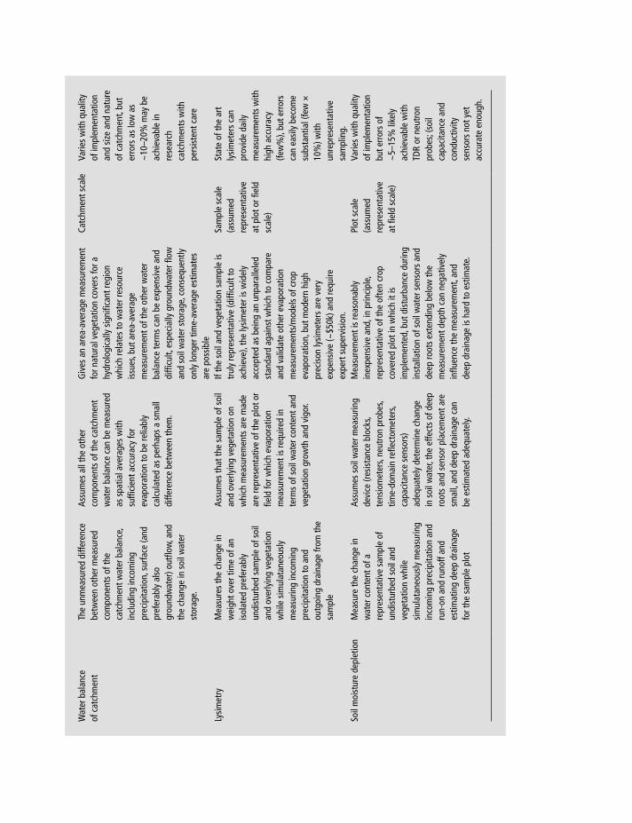
Wat
er b
alan
ce
of c
atch
men
tTh
e un
mea
sure
d di
ffere
nce
betw
een
othe
r mea
sure
d co
mpo
nent
s of
the
catc
hmen
t wat
er b
alan
ce,
incl
udin
g in
com
ing
prec
ipita
tion,
sur
face
(and
pr
efer
ably
als
o gr
ound
wat
er) o
utflo
w, a
nd
the
chan
ge in
soi
l wat
er
stor
age.
Assu
mes
all
the
othe
r co
mpo
nent
s of
the
catc
hmen
t w
ater
bal
ance
can
be
mea
sure
d as
spa
tial a
vera
ges
with
su
ffici
ent a
ccur
acy
for
evap
orat
ion
to b
e re
liabl
y ca
lcul
ated
as
perh
aps
a sm
all
diffe
renc
e be
twee
n th
em.
Giv
es a
n ar
ea-a
vera
ge m
easu
rem
ent
for n
atur
al v
eget
atio
n co
vers
for a
hy
drol
ogic
ally
sig
nific
ant r
egio
n w
hich
rela
tes
to w
ater
reso
urce
is
sues
, but
are
a-av
erag
e m
easu
rem
ent o
f the
oth
er w
ater
ba
lanc
e te
rms
can
be e
xpen
sive
and
di
fficu
lt, e
spec
ially
gro
undw
ater
flow
an
d so
il w
ater
sto
rage
, con
sequ
ently
on
ly lo
nger
tim
e-av
erag
e es
timat
es
are
poss
ible
Catc
hmen
t sca
leVa
ries
with
qua
lity
of im
plem
enta
tion
and
size
and
nat
ure
of c
atch
men
t, bu
t er
rors
as
low
as
~10
–20%
may
be
achi
evab
le in
re
sear
chca
tchm
ents
with
pe
rsis
tent
car
e
Lysi
met
ryM
easu
res
the
chan
ge in
w
eigh
t ove
r tim
e of
an
isol
ated
pre
fera
bly
undi
stur
bed
sam
ple
of s
oil
and
over
lyin
g ve
geta
tion
whi
le s
imul
atan
eous
ly
mea
surin
g in
com
ing
prec
ipita
tion
to a
nd
outg
oing
dra
inag
e fro
m th
e sa
mpl
e
Assu
mes
that
the
sam
ple
of s
oil
and
over
lyin
g ve
geta
tion
on
whi
ch m
easu
rem
ents
are
mad
e ar
e re
pres
enta
tive
of th
e pl
ot o
r fie
ld fo
r whi
ch e
vapo
ratio
n m
easu
rem
ent i
s re
quire
d in
te
rms
of s
oil w
ater
con
tent
and
ve
geta
tion
grow
th a
nd v
igor
.
If th
e so
il an
d ve
geta
tion
sam
ple
is
trul
y re
pres
enta
tive
(diff
icul
t to
achi
eve)
, the
lysi
met
er is
wid
ely
acce
pted
as
bein
g an
unp
aral
lele
d st
anda
rd a
gain
st w
hich
to c
ompa
re
and
valid
ate
othe
r eva
pora
tion
mea
sure
men
ts/m
odel
s of
cro
p ev
apor
atio
n, b
ut m
oder
n hi
gh
prec
ison
lysi
met
ers
are
very
ex
pens
ive
(~$5
0k) a
nd re
quire
ex
pert
sup
ervi
sion
.
Sam
ple
scal
e (a
ssum
edre
pres
enta
tive
at p
lot o
r fie
ld
scal
e)
Stat
e of
the
art
lysi
met
ers
can
prov
ide
daily
m
easu
rem
ents
with
hi
gh a
ccur
acy
(few
%),
but e
rror
s ca
n ea
sily
bec
ome
subs
tant
ial (
few
×
10%
) with
un
repr
esen
tativ
esa
mpl
ing.
Soil
moi
stur
e de
plet
ion
Mea
sure
the
chan
ge in
w
ater
con
tent
of a
re
pres
enta
tive
sam
ple
of
undi
stur
bed
soil
and
vege
tatio
n w
hile
si
mul
atan
eous
ly m
easu
ring
inco
min
g pr
ecip
itatio
n an
d ru
n-on
and
runo
ff an
d es
timat
ing
deep
dra
inag
e fo
r the
sam
ple
plot
Assu
mes
soi
l wat
er m
easu
ring
devi
ce (r
esis
tanc
e bl
ocks
, te
nsio
met
ers,
neut
ron
prob
es,
time-
dom
ain
refle
ctom
eter
s, ca
paci
tanc
e se
nsor
s)
adeq
uate
ly d
eter
min
e ch
ange
in
soi
l wat
er, t
he e
ffect
s of
dee
p ro
ots
and
sens
or p
lace
men
t are
sm
all,
and
deep
dra
inag
e ca
n be
est
imat
ed a
dequ
atel
y.
Mea
sure
men
t is
reas
onab
ly
inex
pens
ive
and,
in p
rinci
ple,
re
pres
enta
tive
of th
e of
ten
crop
co
vere
d pl
ot in
whi
ch it
is
impl
emen
ted,
but
dis
turb
ance
dur
ing
inst
alla
tion
of s
oil w
ater
sen
sors
and
de
ep ro
ots
exte
ndin
g be
low
the
mea
sure
men
t dep
th c
an n
egat
ivel
y in
fluen
ce th
e m
easu
rem
ent,
and
deep
dra
inag
e is
har
d to
est
imat
e.
Plot
sca
le
(ass
umed
repr
esen
tativ
eat
fiel
d sc
ale)
Varie
s w
ith q
ualit
y of
impl
emen
tatio
n bu
t err
ors
of
~5–
15%
like
ly
achi
evab
le w
ith
TDR
or n
eutr
on
prob
es; (
soil
capa
cita
nce
and
cond
uctiv
ityse
nsor
s no
t yet
ac
cura
te e
noug
h.
Shuttleworth_c07.indd 93Shuttleworth_c07.indd 93 11/3/2011 6:31:16 PM11/3/2011 6:31:16 PM
94 Measuring Surface Heat Fluxes
Important points in this chapter
● Measuring solar radiation: either estimated from cloud cover (reported by
an observer, or from a Campbell-Stokes recorder that focuses the Sun’s rays
to burn a card when skies are clear); or measured using a Thermoelectric
pyranometer (from the heating it induces on a blackened surface), or a
Photoelectric pyranometer (from the electrical output, from a silicone voltaic
detector, that it generates).
● Measuring net radiation: either measured as the difference in temperature
between blackened surfaces using a thermopile in a net radiometer, or by
measuring all four components of net radiation separately using two
pyranometers to measure (upward and downward) solar radiation and
two pyrgeometers to measure (upward and downward) longwave
radiation.
● Measuring soil heat flux: measured using the temperature difference across
a soil heat flux plate (a disk a few centimeters in diameter, a few millimeters
thick, with thermal conductivity similar to soil) inserted typically ~5 cm
below ground, with thermometers above to estimate flux loss in the soil
between the surface and plate.
● Micrometeorological measurement of latent and sensible heat: two
techniques remain in common use – both involve deploying sensors meters
or tens of meters above the ground.
— Bowen ratio/energy budget method. H and lE are deduced by simul-
taneously measuring (a) all the other components of the surface energy
budget, to determine the sum of H and lE; and (b) the gradients of
temperature (strictly virtual potential temperature) and humidity (often
measured as vapor pressure), to determine the ratio of H to lE. Individual
values are calculated from the sum and ratio of the two. Sometimes, when
gradients are small, accuracy is improved by interchanging sensors
between levels or ducting air from different levels alternately to a common
sensor.
— Eddy correlation method. H and lE are deduced by multiplying the
instantaneous fluctuation in vertical wind speed with the instantaneous
fluctuation in the volumetric heat content of the air to give the
instantaneous value of H, and with the instantaneous fluctuation in
the volumetric latent heat content of the air to give the instantaneous
value lE. Time-average values are found by integrating these
instantaneous flux values. Rapid response sensors with stable
calibration are required, these typically being interrogated several
times per second.
● Integrated water loss measurement of evaporation: involves defining a sam-
ple of the evaporating surface for which all the water entering or leaving can
be measured over the sampling period. Common measurements include the
following:
Shuttleworth_c07.indd 94Shuttleworth_c07.indd 94 11/3/2011 6:31:16 PM11/3/2011 6:31:16 PM
Measuring Surface Heat Fluxes 95
— Evaporation pans. The measured evaporation from a sample of water
held in a prescribed container (e.g., the ‘Class A’ pan) may be used as an
indication of that from nearby surfaces such as crops and lakes, but
requires correction using an empirical pan coefficient in the range 0.3–1.0
(but usually 0.65–0.85).
— Watersheds and lakes. Evaporation may be inferred from the measured
water balance of watersheds and lakes, but this is difficult because it is
deduced as a small residual in a water balance in which other terms
dominate, so errors may be 20–30%.
— Lysimeters. Evaporation is determined from detailed measurements of
the water balance for a sample of soil and vegetation that is representative
of its surroundings, but ensuring this can be a challenge. High quality
weighing lysimeters are considered the (albeit expensive) standard
against which alternatives can be validated.
— Soil moisture depletion. The measurements of precipitation and the
change in the soil moisture stored in the soil profile (measured using
neutron probes, capacitance probes, time-domain reflectometers, etc.)
can be used to estimate evaporation.
References
Campbell Scientific (1987) Bowen Ratio Instrumentation, Campbell Scientific, Logan, Utah,
online at: http://www.campbellsci.com/documents/manuals/bowen.pdf.
Fairmount Weather Systems (2010) Meldreth, Hertfordshire, UK, online at: http://www.
fairmountweather.com/.
Federer, C.A. & Tanner, C.B. (1966) Sensors for measuring light available for photosynthe-
sis. Ecology, 47, 654–7.
Kipp and Zonen (2010) Delft, The Netherlands, online at: http://www.kippzonen.
com/?category/111/Home.aspx.
LI-COR Environmental (2010) Lincoln, Nebraska, online at: http://www.licor.com/env/
Products/Sensors/200/li200_description.jsp.
McCaughey, J.H. (1981) A reversing temperature-difference measurement system for
Bowen ratio determination. Boundary-Layer Meteorology, 21 (1), 47–55.
Shuttleworth, W.J. (1993) Evaporation. In: Handbook of Hydrology (ed. D. Maidment),
pp. 4.1–4.53. McGraw-Hill, New York.
Shuttleworth_c07.indd 95Shuttleworth_c07.indd 95 11/3/2011 6:31:16 PM11/3/2011 6:31:16 PM
Introduction
Among the many acronyms used by scientists arguably ‘GCM’ is currently the best
recognized and most widely used, not only by meteorologists and hydrometeor-
ologists but also by other scientific disciplines, politicians and policymakers, and
by members of the public. Many non-experts think the acronym is shorthand for
‘Global Climate Model’ because it is widespread interest in global climate change
that has fostered its popularity. But the acronym predates this widespread interest
and in reality it is shorthand for General Circulation Model.
This chapter is written to provide an introduction to this aspect of present-day
atmospheric science for hydrometeorologists who will not necessarily become
experts in the specialized field of atmospheric modeling, but who need to be
familiar with the basic nature of GCMs and their strengths and shortcomings.
Because changes in the hydroclimate of the Earth are predicted, hydroclimatolo-
gists and hydrometeorologists need a basic understanding of the models used to
make such predictions.
What are General Circulation Models?
General Circulation Models are complex computer programs written to
describe how the air in the atmosphere moves, or circulates, around the globe.
To do this they include in their code the equations that describe the conserva-
tion and movement of momentum, energy, and the mass of atmospheric con-
stituents (including water vapor) which are discussed in later chapters. They
8 General Circulation Models
Terrestrial Hydrometeorology, First Edition. W. James Shuttleworth.
© 2012 John Wiley & Sons, Ltd. Published 2012 by John Wiley & Sons, Ltd.
Shuttleworth_c08.indd 96Shuttleworth_c08.indd 96 11/3/2011 6:30:44 PM11/3/2011 6:30:44 PM

General Circulation Models 97
also include equations describing the processes that transfer momentum,
energy, and mass into and out of the atmosphere from oceans and continents,
and the energy incoming to the atmosphere as shortwave radiation from the
Sun and outgoing as longwave radiation to deep space. Aspects of these
processes were discussed in earlier chapters. GCMs also include in their
code equations that describe the evolution with time of atmospheric constitu-
ents. This may require description of chemical reactions but much more
commonly it requires that the phase changes for atmospheric constituents are
described, the description of the phase changes of water being the most
important need.
When describing the computational mechanics that GCMs use to describe the
atmosphere, it is helpful first to draw an analogy with the computer programs
that are set up to manage bank accounts. GCMs manage atmospheric bank
accounts for volumes of atmosphere each of which is defined by the area of the
Earth’s surface it overlies (specified as lying between latitude and longitude limits)
and by a height range above the ground. Although not strictly cubes, one might
visualize these volumes as being equivalent to bricks which when cemented
together form the whole atmosphere. The bank accounts maintained by the GCM
for each volume of atmosphere contain wealth in several different ‘currencies’, the
most important being the energy, momentum, and mass of atmospheric
constituents.
Extending the bank account analogy one step further, at regular intervals a
banking program would update the bank accounts it maintains to reflect changes
in the amount held in each currency in each account as a result of financial
transactions between them, and the interest earned on deposits and value lost by
inflation. In a broadly similar way, having built this basic descriptive framework
for the atmosphere, at regular intervals GCMs represent how much energy,
momentum, and mass is moved between the volumes of atmosphere it has defined
and the extent to which there are internally generated increases or decreases
within the volume.
Figure 8.1 illustrates how a GCM might partition the atmosphere into
segments and some of the exchanges and internal processes that are represented
in the model. The size of the areas of atmosphere represented in each column
of air, which is usually called the grid scale of the GCM, and the height range of
each volume within each column are mainly determined by computational
constraints. The computer memory available to store values of atmospheric
variables for each volume element in part determines the size of the volume
elements selected. However, just as important, if the computer program is to
remain stable, the time step at which updates are made to the variables in each
volume element falls rapidly as the grid scale and height ranges decrease.
Hence, the run time of atmospheric simulations also rapidly increases as the
grid scale and height ranges decrease. In practice, for stable operation a time
step of 20–30 minutes is required when GCMs have a grid scale of a few hundred
kilometers.
Shuttleworth_c08.indd 97Shuttleworth_c08.indd 97 11/3/2011 6:30:45 PM11/3/2011 6:30:45 PM
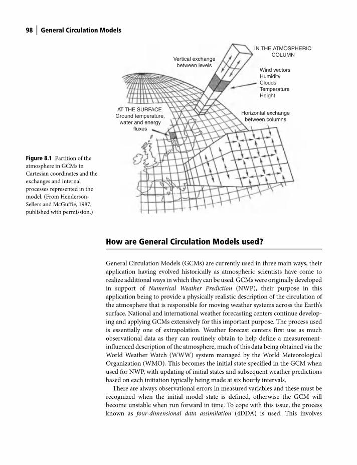
98 General Circulation Models
IN THE ATMOSPHERICCOLUMN
Wind vectorsHumidityCloudsTemperatureHeight
Vertical exchangebetween levels
AT THE SURFACEGround temperature,
water and energyfluxes
Horizontal exchangebetween columns
Figure 8.1 Partition of the
atmosphere in GCMs in
Cartesian coordinates and the
exchanges and internal
processes represented in the
model. (From Henderson-
Sellers and McGuffie, 1987,
published with permission.)
How are General Circulation Models used?
General Circulation Models (GCMs) are currently used in three main ways, their
application having evolved historically as atmospheric scientists have come to
realize additional ways in which they can be used. GCMs were originally developed
in support of Numerical Weather Prediction (NWP), their purpose in this
application being to provide a physically realistic description of the circulation of
the atmosphere that is responsible for moving weather systems across the Earth’s
surface. National and international weather forecasting centers continue develop-
ing and applying GCMs extensively for this important purpose. The process used
is essentially one of extrapolation. Weather forecast centers first use as much
observational data as they can routinely obtain to help define a measurement-
influenced description of the atmosphere, much of this data being obtained via the
World Weather Watch (WWW) system managed by the World Meteorological
Organization (WMO). This becomes the initial state specified in the GCM when
used for NWP, with updating of initial states and subsequent weather predictions
based on each initiation typically being made at six hourly intervals.
There are always observational errors in measured variables and these must be
recognized when the initial model state is defined, otherwise the GCM will
become unstable when run forward in time. To cope with this issue, the process
known as four-dimensional data assimilation (4DDA) is used. This involves
Shuttleworth_c08.indd 98Shuttleworth_c08.indd 98 11/3/2011 6:30:45 PM11/3/2011 6:30:45 PM
General Circulation Models 99
making a compromise between the model-calculated fields defined by the GCM at
the time of the initiation (which are, of course, consistent with the equations used
in the GCM), and any observations available at that time. The values of the weather
variables specified in the initial state of the GCM thus become a weighted average
of that predicted by the GCM based on an earlier initiation and those currently
observed. Plausible values are assumed for errors in the observational data and
model calculated values, and these are used to define the weighted average initial
fields. If the observed values are substantially different to model calculated values
they are rejected as implausible and not used in the initiation.
The GCM is then run forward in time for some days ahead and in this way
numerical predictions of actual weather made for the future. In practice, there are
always shortcomings in the description of the atmosphere represented in the GCM
not least because the representation is made at grid scale using approximate
equations that parameterize processes that occur at much smaller scale.
Consequently, the accuracy of weather predictions degrades with time ahead.
Currently GCMs used for weather prediction can make reasonable predictions for
a few days ahead, and some weather centers attempt forward look predictions for
as long as 8–10 days ahead. Thus, when used for NWP, GCMs extrapolate observa-
tions forward in time using a physically realistic representation of atmospheric
circulation to predict the actual future weather for periods of several days ahead.
Some time ago it was realized that the process of NWP could provide an
important byproduct. The six hourly initiation process using data assimilation
calculates values of the meteorological variables used in the GCM everywhere in
the atmosphere. These values are in significant part based on model predictions,
but they are at least in part influenced by observations. Globally available fields of
weather variables cannot be routinely obtained at regular six hourly intervals in
any other way. But they are needed, and for this reason model-calculated data
based on the assimilation of observations into GCMs have now become widely
used as a source of data in their own right. Thus, the initiation fields of GCMs used
for NWPs are often stored and can be made available as a data source which has
the advantage of being broadly consistent with the laws of atmospheric physics (to
the extent these are represented in the GCM), while also reflecting relevant
observations available at the time of initiation to the extent allowed by the data
assimilation process.
One feature of such model-calculated data when provided as time series is that
the amount and nature of observational data that influence the data product
through data assimilation can change with time. Consequently, the relative
influence of observations versus model in the data also changes with time. Over
the years weather forecast centers have sought to use more and more observations
to better define the initial states used for their forecasts, and the amount of remote
sensing data so used has also greatly increased. As a result more recent
model-calculated data are arguably a better reflection of reality. An important
shortcoming of model-calculated data arises because weather forecast centers are
always striving to improve the realism with which atmospheric processes are
represented in their model. Consequently, improved versions of the GCMs used
Shuttleworth_c08.indd 99Shuttleworth_c08.indd 99 11/3/2011 6:30:45 PM11/3/2011 6:30:45 PM
100 General Circulation Models
for NWP are therefore adopted and applied. Because the data delivered by data
assimilation is influenced by the nature of the GCM used, this means there are
discontinuities in the derived global data sets associated with model changes. For
this reason, some major modeling centers have deliberately created model-
calculated data sets by applying consistent data assimilation procedures to
historical observational data using the same recent model to provide more
consistent data series. These data are called reanalysis data. Thus, when GCMs are
used to create model-calculated reanalysis data, a consistent data assimilation
procedure is used with the same version of the GCM to calculated globally available
data sets of weather variables from historical data records.
As experience in the use of GCMs in NWP grew, confidence also grew that
although their ability to predict actual weather decayed after several days, their
ability to make reasonable predictions of the statistics of weather, i.e., climate, at a
particular place was retained. This confidence sparked a whole new branch of
atmospheric science, namely climate prediction. When GCMs are used in this way,
they are used to predict a sequence of weather events which, it is assumed, is
representative of those that will occur, or that would occur given prescribed
changes in the factors that influence weather. Among the factors that may change
future climate are the concentration of gases that are involved in the absorption
and emission of radiation in the atmosphere and the nature of the vegetation
covering land areas of the globe.
Thus, climate prediction involves running GCMs for longer periods than weather
predictions, at least for seasons and commonly for several years, decades, centuries,
and even millennia. An initial global field of weather variables must still be provided
when a GCM is used for climate prediction and different patterns of simulated
weather sequences will result for different initiation fields. For this reason, climate
predictions are now usually made with several different initiation fields selected
(perhaps randomly) to be typical from those made available by operational NWP.
The resulting suite of predictions given by a GCM with different initiation fields is
called an ensemble. The mean of such an ensemble might be adopted as the average
climate prediction for the GCM, and the variability of the ensemble considered a
measure of the GCM dependent accuracy of the prediction. Thus, when GCMs are
used for climate prediction the purpose is to simulate the average statistics of weather
across the globe over long periods and to quantify the changes induced in these statistics
in response to prescribed changes in the influences that determine weather.
How do General Circulation Models work?
Sequence of operations
The operational sequence used in running GCMs is illustrated in Fig. 8.2. As
described in the previous section, the first step is to define an initial state for all of
the variables whose evolution is being simulated using 4DDA.
Shuttleworth_c08.indd 100Shuttleworth_c08.indd 100 11/3/2011 6:30:45 PM11/3/2011 6:30:45 PM
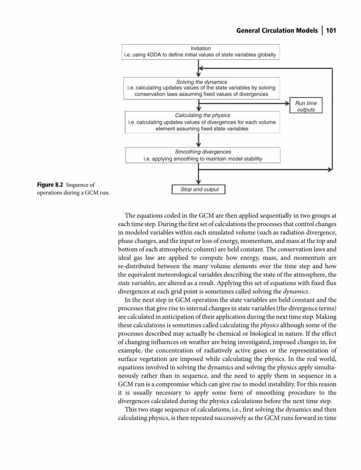
General Circulation Models 101
The equations coded in the GCM are then applied sequentially in two groups at
each time step. During the first set of calculations the processes that control changes
in modeled variables within each simulated volume (such as radiation divergence,
phase changes, and the input or loss of energy, momentum, and mass at the top and
bottom of each atmospheric column) are held constant. The conservation laws and
ideal gas law are applied to compute how energy, mass, and momentum are
re-distributed between the many volume elements over the time step and how
the equivalent meteorological variables describing the state of the atmosphere, the
state variables, are altered as a result. Applying this set of equations with fixed flux
divergences at each grid point is sometimes called solving the dynamics.
In the next step in GCM operation the state variables are held constant and the
processes that give rise to internal changes in state variables (the divergence terms)
are calculated in anticipation of their application during the next time step. Making
these calculations is sometimes called calculating the physics although some of the
processes described may actually be chemical or biological in nature. If the effect
of changing influences on weather are being investigated, imposed changes in, for
example, the concentration of radiatively active gases or the representation of
surface vegetation are imposed while calculating the physics. In the real world,
equations involved in solving the dynamics and solving the physics apply simulta-
neously rather than in sequence, and the need to apply them in sequence in a
GCM run is a compromise which can give rise to model instability. For this reason
it is usually necessary to apply some form of smoothing procedure to the
divergences calculated during the physics calculations before the next time step.
This two stage sequence of calculations, i.e., first solving the dynamics and then
calculating physics, is then repeated successively as the GCM runs forward in time
Initiationi.e. using 4DDA to define initial values of state variables globally
Solving the dynamicsi.e. calculating updates values of the state variables by solving
conservation laws assuming fixed values of divergences
Calculating the physicsi.e. calculating updates values of divergences for each volume
element assuming fixed state variables
Smoothing divergences
Stop and output
i.e. applying smoothing to maintain model stability
Run timeoutputs
Figure 8.2 Sequence of
operations during a GCM run.
Shuttleworth_c08.indd 101Shuttleworth_c08.indd 101 11/3/2011 6:30:45 PM11/3/2011 6:30:45 PM

102 General Circulation Models
until the model run reaches some predefined stopping point. Selected calculated
fields are output as the model proceeds that provide the required description of
the evolving atmosphere.
Solving the dynamics
GCMs use two different ways to store state variables. The first is that illustrated in
Fig. 8.1 in which the state variables are stored as individual values of atmospheric
variables for each of the defined atmospheric volume elements as specified by lines
of latitude and longitude using (currently 0.5° to 5°) grid scale and the (currently
5–25 m) vertical height ranges. When this is done, state variables are said to be
stored on a Cartesian Grid.
The alternative way to store the values of state variables is on a Spectral Grid, see
Fig. 8.3. When this is done, instead of storing individual values of atmospheric
Transformation to grid space samples fieldaround zones of Iatitude and longitude
Each atmospheric layer heldand moved in spectral space
Spectral truncationrestricts information
Each surface is transformedinto sampled grid space
representation
sp nplatitude
longitude
Vertical exchangesin grid space
0� 360�
Surface fluxes arecomputed in grid space
(2)
(1)
(3)
(4)
Figure 8.3 Representation of
the atmosphere in GCMs in
spectral coordinates and the
interchange Cartesian
coordinates required to
calculate the physics. (From
Henderson-Sellers and
McGuffie, 1987, published
with permission.)
Shuttleworth_c08.indd 102Shuttleworth_c08.indd 102 11/3/2011 6:30:45 PM11/3/2011 6:30:45 PM
General Circulation Models 103
variables, the GCM stores information on the global pattern of state variables at
each level in the atmosphere in the form of a Fourier series. In this series, each
term has a wavelength an integral multiple of which corresponds to the distance
around the Earth. By expressing the longitudinal distribution of state variables in
this way between time steps, it is possible to capture most (but not all) of the spatial
variability using less computer storage by truncating the Fourier series after a
specified number of wavelengths. The number of wavelengths before truncation
varies with the application of the GCMs, longer climate prediction runs having
truncation earlier than shorter NWP runs. When using a spectral grid, movement
within each vertical layer of the atmosphere can be calculated in spectral space and
this computation can be efficient. However, vertical movement and calculating the
physics for each atmospheric column requires transposition of the state variables
into coordinate space. Using a spectral grid is most effective when describing state
variables that vary smoothly across the globe. Truncating the Fourier series in a
spectral description can give rise to artificial wavelike features and unrealistic
divergences and, as computer memory becomes more available, the technical
advantages of using a spectral description of state variables become less
significant.
Calculating the physics
Calculation of the physics is made for each atmospheric column extending from
the surface upward to a defined level, which is regarded as being the top of the
atmosphere. The GCM code contains subroutines that compute the divergence of
energy, momentum and the mass of atmospheric constituents, the surface
exchanges of these variables, and buoyant exchanges between cells at different
levels in this column. Typically GCMs will include at least the following
subroutines.
● Radiation scheme: The radiation transfer scheme calculates the propagation
and reflection of shortwave and longwave radiation through each layer in the
atmospheric column from the modeled profiles of temperature, humidity,
cloud amount and the concentration of aerosols, ozone, and radiatively
active gases such as water vapor and carbon dioxide.
● Boundary-layer scheme: The boundary-layer scheme uses first order, height-
integrated representations of the surface energy and momentum exchanges
between the lowest model level represented in the GCM and the ground,
based on the modeled vertical gradients of the variables which control these
exchanges.
● Surface-parameterization scheme: The surface-parameterization scheme pro-
vides a description of shortwave and longwave exchange, momentum cap-
ture, and how the available energy at the surface is shared as heat fluxes
for sea, sea-ice, land-ice, snow-covered land, and several snow-free
land-cover types.
Shuttleworth_c08.indd 103Shuttleworth_c08.indd 103 11/3/2011 6:30:46 PM11/3/2011 6:30:46 PM

104 General Circulation Models
● Convection scheme: The convection scheme computes the exchange of buoy-
ant thermals and compensation flows between modeled layers, and calcu-
lates the amount of convective precipitation generated as these thermals rise
and cool.
● Large-scale precipitation scheme: The large-scale precipitation scheme
calculates if each of the modeled layers has become saturated and removes
any excess water as rain, if the air temperature is greater than freezing point,
or as frozen precipitation, if the air temperature is less than freezing point.
Intergovernmental Panel on Climate Change (IPCC)
The Intergovernmental Panel on Climate Change (IPCC) is a scientific
intergovernmental body tasked to evaluate the risk of climate change caused by
human activity. The panel was established in 1988 by the World Meteorological
Organization (WMO) and the United Nations Environment Programme (UNEP),
two organizations of the United Nations. The IPCC shared the 2007 Nobel Peace
Prize.
The IPCC does not carry out research, nor does it monitor climate or related
phenomena. A main activity of the IPCC is publishing special reports on topics
relevant to the implementation of the UN Framework Convention on Climate
Change, an international treaty that acknowledges the possibility of harmful
climate change. The IPCC bases its assessment on the most recent scientific,
technical and socio-economic information produced worldwide relevant to the
understanding of climate change. IPCC reports are widely cited in almost any
debate related to climate change.
The IPCC First Assessment Report appeared in 1990 with a supplementary
report in 1992, and there have been subsequent reports in 1995, 2001 and 2007.
The key conclusions of the most recent IPCC report (IPCC, 2007) are as
follows:
● Warming of the climate system is unequivocal.
● Most of the observed increase in globally averaged temperature since the
mid-twentieth century is very likely due to the observed increase in anthro-
pogenic (human-caused) greenhouse gas concentrations.
● Anthropogenic warming and sea-level rise would continue for centuries due
to the timescales associated with climate processes and feedbacks, even if
greenhouse gas concentrations were to be stabilized, although the likely
amount of temperature and sea-level rise varies greatly depending on the
intensity of fossil fuel burning during the next century.
● The probability that this is caused by natural climatic processes alone is less
than 5%.
● World temperatures could rise by between 1.1 and 6.4°C (2.0 and 11.5°F)
during the twenty-first century, and:
Shuttleworth_c08.indd 104Shuttleworth_c08.indd 104 11/3/2011 6:30:46 PM11/3/2011 6:30:46 PM

General Circulation Models 105
— sea levels will probably rise by 18 to 59 cm (7.08 to 23.22 in).
— there is a confidence level >90% that there will be more frequent warm
spells, heat waves and heavy rainfall.
— there is a confidence level >66% that there will be an increase in droughts,
tropical cyclones and extreme high tides.
● Both past and future anthropogenic carbon dioxide emissions will continue
to contribute to warming and sea-level rise for more than a millennium.
● Global atmospheric concentrations of carbon dioxide, methane, and nitrous
oxide have increased markedly as a result of human activities since 1750 and
now far exceed pre-industrial values over the past 650,000 years.
In IPCC statements ‘most’ means greater than 50%, ‘likely’ means at least a 66%
likelihood, and ‘very likely’ means at least a 90% likelihood.
Important points in this chapter
● What are General Circulation Models (GCMs)? Computer programs which
describe atmosphere circulation using equations that portray conservation
and movement of atmospheric constituents, incoming solar radiation and
outgoing longwave radiation, and transfers between the atmosphere and
oceans and continents. Currently GCMs describe changes in the atmosphere
every 20–30 minutes at points separated by 10s–100s of kilometers in the
horizontal and by 10s-1000s of meters in the vertical.
● How are GCMs used? To give:
— numerical weather prediction (NWP) in which an observation-based
description of the current atmosphere is extrapolated forward for several
(typically 3–8) days to calculate the actual weather likely to occur over
this period.
— globally-available atmospheric ‘data’ provided by GCMs as a byproduct of
the process necessary to define the initial state of the atmosphere prior to
an NWP run, with four-dimensional data assimilation used to define a
weighted average description between that previously predicted by the
GCM and all relevant observations available at the time of initiation.
— climate prediction in which it is assumed that, although they are not able
to predict actual weather for more than a few days, GCMs are able to
predict the statistics of weather, i.e., climate, for periods up to many cen-
turies ahead.
● How do GCMs Work? Once an initial state of the atmosphere has been
defined, equations coded in the GCM are applied at each time step in two
groups sequentially;
— the dynamics, equations that control the model’s state variables solved
assuming fixed values for variables (such as flux divergences) that deter-
mine changes in state variables; and
Shuttleworth_c08.indd 105Shuttleworth_c08.indd 105 11/3/2011 6:30:46 PM11/3/2011 6:30:46 PM
106 General Circulation Models
— the physics, equations that calculate the controlling values to be applied in
the subsequent dynamics, these being calculated using the most recently
updated state variables.
The dynamics are then again solved and the physics re-calculated, and so on
until the run is complete.
● Solving the dynamics: GCMs use two ways to store and solve state variables,
either as individual values for each volume elements stored in a Cartesian
Grid, or on a Spectral Grid as a (truncated) series of Fourier coefficients that
describe the longitudinal variation in state variables.
● Calculating the physics: the divergence of state variables is calculated
throughout the atmospheric column, along with the buoyant exchanges
between cells at different levels and the surface exchanges of state variables
using (at least) the following subroutines: (a) Radiation scheme; (b) Boundary-
layer scheme; (c) Surface-parameterization scheme, (d) Convection scheme;
and (e) Large-scale precipitation scheme.
● Intergovernmental Panel on Climate Change (IPCC): an intergovernmental
body tasked with evaluating the risk of climate change caused by human
activity based on the most recent scientific, technical and socio-economic
information produced worldwide relevant to the understanding of climate
change. The 2007 IPCC Assessment Report stated that warming of the
climate system is unequivocal, and most of the observed increase in globally
averaged temperatures since the mid-twentieth century is very likely due to
the observed increase in anthropogenic (human-caused) greenhouse gas
concentrations.
References
Henderson-Sellers, A. & McGuffie, K. (1987) Climate Modelling Primer. Wiley & Sons,
Chichester, UK.
IPCC (2007) The Intergovernmental Panel on Climate Change, World Meteorological
Organization, Geneva 2, Switzerland, online at http://www.ipcc.ch/
Shuttleworth_c08.indd 106Shuttleworth_c08.indd 106 11/3/2011 6:30:46 PM11/3/2011 6:30:46 PM
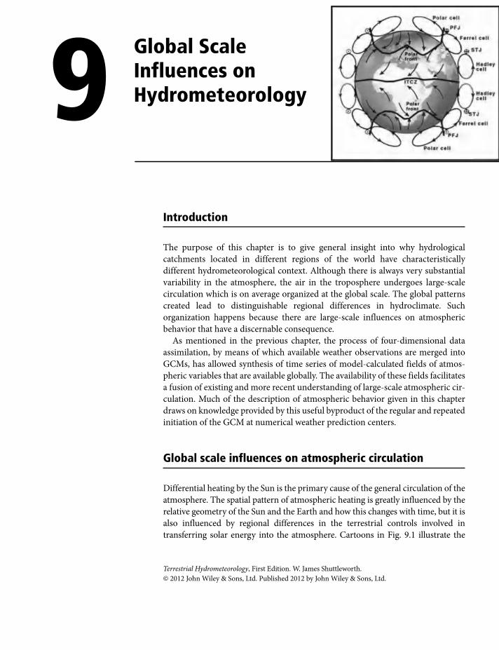
Introduction
The purpose of this chapter is to give general insight into why hydrological
catchments located in different regions of the world have characteristically
different hydrometeorological context. Although there is always very substantial
variability in the atmosphere, the air in the troposphere undergoes large-scale
circulation which is on average organized at the global scale. The global patterns
created lead to distinguishable regional differences in hydroclimate. Such
organization happens because there are large-scale influences on atmospheric
behavior that have a discernable consequence.
As mentioned in the previous chapter, the process of four-dimensional data
assimilation, by means of which available weather observations are merged into
GCMs, has allowed synthesis of time series of model-calculated fields of atmos-
pheric variables that are available globally. The availability of these fields facilitates
a fusion of existing and more recent understanding of large-scale atmospheric cir-
culation. Much of the description of atmospheric behavior given in this chapter
draws on knowledge provided by this useful byproduct of the regular and repeated
initiation of the GCM at numerical weather prediction centers.
Global scale influences on atmospheric circulation
Differential heating by the Sun is the primary cause of the general circulation of the
atmosphere. The spatial pattern of atmospheric heating is greatly influenced by the
relative geometry of the Sun and the Earth and how this changes with time, but it is
also influenced by regional differences in the terrestrial controls involved in
transferring solar energy into the atmosphere. Cartoons in Fig. 9.1 illustrate the
9 Global Scale Influences on Hydrometeorology
Terrestrial Hydrometeorology, First Edition. W. James Shuttleworth.
© 2012 John Wiley & Sons, Ltd. Published 2012 by John Wiley & Sons, Ltd.
Shuttleworth_c09.indd 107Shuttleworth_c09.indd 107 11/3/2011 6:30:29 PM11/3/2011 6:30:29 PM
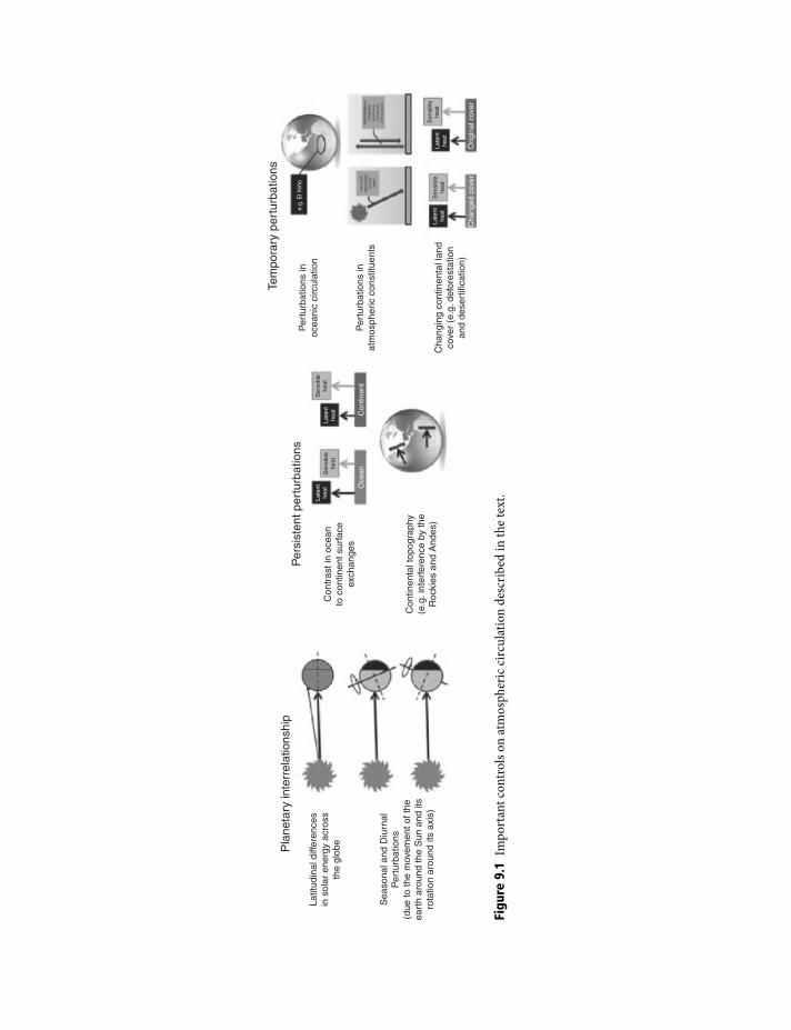
Pla
neta
ry in
terr
elat
ions
hip
Per
sist
ent p
ertu
rbat
ions
Tem
pora
ry p
ertu
rbat
ions
Latit
udin
al d
iffer
ence
sin
sol
ar e
nerg
y ac
ross
the
glob
eC
ontr
ast i
n oc
ean
to c
ontin
ent s
urfa
ceex
chan
ges
Per
turb
atio
ns in
ocea
nic
circ
ulat
ion
Per
turb
atio
ns in
atm
osph
eric
con
stitu
ents
Cha
ngin
g co
ntin
enta
l lan
dco
ver
(e.g
. def
ores
tatio
nan
d de
sert
ifica
tion)
Late
nthe
atLa
tent
heat
Sen
sibl
ehe
at
Sen
sibl
ehe
at
Oce
anC
ontin
ent
Late
nthe
atLa
tent
heat
Sen
sibl
ehe
at
Sen
sibl
ehe
at
Cha
nged
cov
erO
rigin
al c
over
Con
tinen
tal t
opog
raph
y(e
.g. i
nter
fere
nce
by th
eR
ocki
es a
nd A
ndes
)
Sea
sona
l and
Diu
rnal
Per
turb
atio
ns(d
ue to
the
mov
emen
t of t
heea
rth
arou
nd th
e S
un a
nd it
sro
tatio
n ar
ound
its
axis
)
e.g.
EI N
iño
Figu
re 9
.1 I
mp
ort
ant
con
tro
ls o
n a
tmo
sph
eric
cir
cula
tio
n d
escr
ibed
in
th
e te
xt.
Shuttleworth_c09.indd 108Shuttleworth_c09.indd 108 11/3/2011 6:30:29 PM11/3/2011 6:30:29 PM

Global Scale Influences on Hydrometeorology 109
most important controls on atmospheric circulation described below. In approximate
descending order of importance, these controls can be classified as follows.
Planetary interrelationship
Latitudinal differences in solar energy input
The Earth rotates around an axis that is (when averaged over the whole year)
perpendicular to the plane in which the Earth moves around the Sun. Consequently,
the solar energy received per unit area is, on average, greatest at the equator and
least at the poles. This difference causes atmospheric circulations that transfer
energy within the moving atmosphere from low to high latitude.
Seasonal perturbations
Because the axis of rotation of the Earth on any particular day is not perpendicular
to the plane in which the Earth moves around the Sun (see Fig. 5.7 and Fig. 9.1),
the latitude where there is most and least solar radiation changes with season. This
results in persistent regular seasonal changes in circulation patterns.
Daily perturbations
The rotation of the Earth means there is a regular diurnal cycle in the longitude at
which there is maximum input of solar radiation. At any latitude, the magnitude
and timing of this daily cycle of energy changes with season.
Persistent perturbations
Contrast in ocean to continent surface exchanges
On average about half of the solar energy reaching the Earth enters the atmosphere
from the Earth’s surface, mainly in the form of surface latent and sensible heat
fluxes. Because water is freely available at the ocean surface but not necessarily at
continental surfaces, there is a characteristic difference in the relative magnitude
of these two different fluxes for these two surfaces. The average aerodynamic
roughness of oceans is also less than that of continents. This contrast in surface
exchanges of energy and momentum influences regional hydroclimate.
Continental topography
Atmospheric circulation mainly occurs in the troposphere. In some locations the
height of continental topography is of the same order as the depth of the troposphere
and this can influence regional flow patterns to some extent, particularly when
topography is organized in mountain chains that lie roughly perpendicular to
atmospheric flow (e.g., the Rockies and Andes).
Shuttleworth_c09.indd 109Shuttleworth_c09.indd 109 11/3/2011 6:30:30 PM11/3/2011 6:30:30 PM
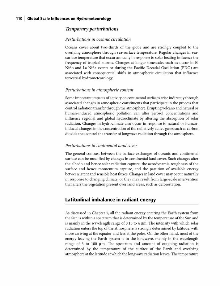
110 Global Scale Influences on Hydrometeorology
Temporary perturbations
Perturbations in oceanic circulation
Oceans cover about two-thirds of the globe and are strongly coupled to the
overlying atmosphere through sea-surface temperature. Regular changes in sea-
surface temperature that occur annually in response to solar heating influence the
frequency of tropical storms. Changes at longer timescales such as occur in El
Niño and La Niña events or during the Pacific Decadal Oscillation (PDO) are
associated with consequential shifts in atmospheric circulation that influence
terrestrial hydrometeorology.
Perturbations in atmospheric content
Some important impacts of activity on continental surfaces arise indirectly through
associated changes in atmospheric constituents that participate in the process that
control radiation transfer through the atmosphere. Erupting volcano and natural or
human-induced atmospheric pollution can alter aerosol concentrations and
influence regional and global hydroclimate by altering the absorption of solar
radiation. Changes in hydroclimate also occur in response to natural or human-
induced changes in the concentration of the radiatively active gases such as carbon
dioxide that control the transfer of longwave radiation through the atmosphere.
Perturbations in continental land cover
The general contrast between the surface exchanges of oceanic and continental
surface can be modified by changes in continental land cover. Such changes alter
the albedo and hence solar radiation capture, the aerodynamic roughness of the
surface and hence momentum capture, and the partition of available energy
between latent and sensible heat fluxes. Changes in land cover may occur naturally
in response to changing climate, or they may result from large-scale intervention
that alters the vegetation present over land areas, such as deforestation.
Latitudinal imbalance in radiant energy
As discussed in Chapter 5, all the radiant energy entering the Earth system from
the Sun is within a spectrum that is determined by the temperature of the Sun and
is mainly in the wavelength range of 0.15 to 4 μm. The intensity with which solar
radiation enters the top of the atmosphere is strongly determined by latitude, with
more arriving at the equator and less at the poles. On the other hand, most of the
energy leaving the Earth system is in the longwave, mainly in the wavelength
range of 3 to 100 μm. The spectrum and amount of outgoing radiation is
determined by the temperature of the surface of the Earth and overlying
atmosphere at the latitude at which the longwave radiation leaves. The temperature
Shuttleworth_c09.indd 110Shuttleworth_c09.indd 110 11/3/2011 6:30:30 PM11/3/2011 6:30:30 PM
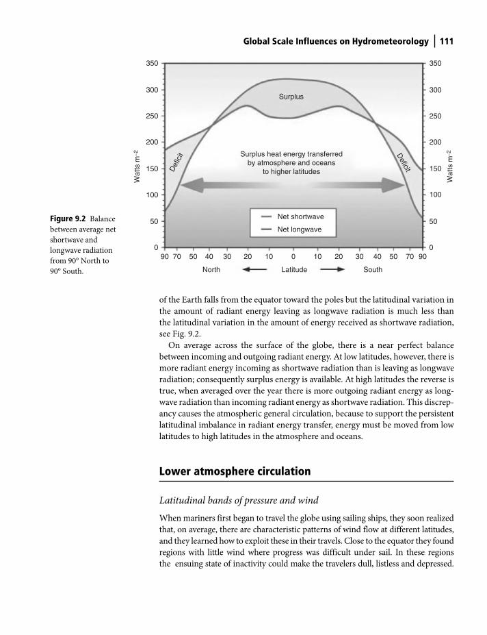
Global Scale Influences on Hydrometeorology 111
of the Earth falls from the equator toward the poles but the latitudinal variation in
the amount of radiant energy leaving as longwave radiation is much less than
the latitudinal variation in the amount of energy received as shortwave radiation,
see Fig. 9.2.
On average across the surface of the globe, there is a near perfect balance
between incoming and outgoing radiant energy. At low latitudes, however, there is
more radiant energy incoming as shortwave radiation than is leaving as longwave
radiation; consequently surplus energy is available. At high latitudes the reverse is
true, when averaged over the year there is more outgoing radiant energy as long-
wave radiation than incoming radiant energy as shortwave radiation. This discrep-
ancy causes the atmospheric general circulation, because to support the persistent
latitudinal imbalance in radiant energy transfer, energy must be moved from low
latitudes to high latitudes in the atmosphere and oceans.
Lower atmosphere circulation
Latitudinal bands of pressure and wind
When mariners first began to travel the globe using sailing ships, they soon realized
that, on average, there are characteristic patterns of wind flow at different latitudes,
and they learned how to exploit these in their travels. Close to the equator they found
regions with little wind where progress was difficult under sail. In these regions
the ensuing state of inactivity could make the travelers dull, listless and depressed.
90900
50
100
150
Wat
ts m
−2200
250
300
350
Wat
ts m
−2
0
50
100
150
200
250
300
350
705070 50 40 30
North South
Net shortwave
Surplus heat energy transferredby atmosphere and oceans
to higher latitudes
Surplus
Def
icit D
eficit
Net longwave
Latitude
403020 2010 100
Figure 9.2 Balance
between average net
shortwave and
longwave radiation
from 90° North to
90° South.
Shuttleworth_c09.indd 111Shuttleworth_c09.indd 111 11/3/2011 6:30:30 PM11/3/2011 6:30:30 PM

112 Global Scale Influences on Hydrometeorology
They called these regions the Doldrums. North or south of the Doldrums the winds
became steadier and were more consistently from the east: southeasterly winds
north of the equator and northeasterly winds south of the equator. These winds were
important because their consistent presence meant international trade using sailing
ships could flourish and they became known as the Trade Winds. At about 30° on
either side of the equator, again there was sometimes little wind. These areas were
called the horse latitudes, because here ships could become becalmed and, on occa-
sion, any horses on board were thrown overboard in order to conserve precious
water. Farther from the equator still, at latitudes near 60°N and 60°S, average winds
became strongly westerly. Pressure shows similar time-average consistent tendencies
with latitude, with low pressure at the equator, high pressure at 30°N and 30°S, low
pressure again at 60°N and 60°S, and higher pressure at the poles, see Fig. 9.3.
Hadley circulation
In the early 1700s, George Hadley, an English lawyer and amateur meteorologist,
argued that solar heating creates upward motion of equatorial air and air from
Mid-latitude cell
Mid-latitude cell
Polar cell
Polar cell
Westerlies
Inter-tropicalconvergence
30�N
30�S
60�S
60�N
0�
Westerlies
High pressure
High pressure
Low pressure
Northeasterly trades
Southeasterly trades
Hadley cell
Hadley cell
Figure 9.3 Variation in time-average wind speed and pressure with latitude.
Shuttleworth_c09.indd 112Shuttleworth_c09.indd 112 11/3/2011 6:30:30 PM11/3/2011 6:30:30 PM
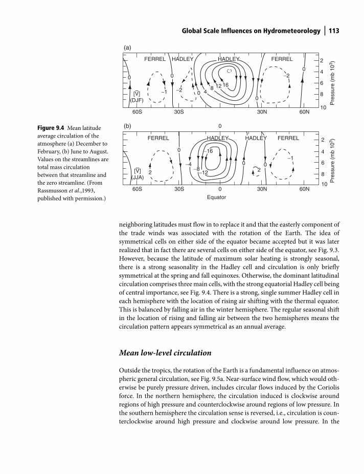
Global Scale Influences on Hydrometeorology 113
neighboring latitudes must flow in to replace it and that the easterly component of
the trade winds was associated with the rotation of the Earth. The idea of
symmetrical cells on either side of the equator became accepted but it was later
realized that in fact there are several cells on either side of the equator, see Fig. 9.3.
However, because the latitude of maximum solar heating is strongly seasonal,
there is a strong seasonality in the Hadley cell and circulation is only briefly
symmetrical at the spring and fall equinoxes. Otherwise, the dominant latitudinal
circulation comprises three main cells, with the strong equatorial Hadley cell being
of central importance, see Fig. 9.4. There is a strong, single summer Hadley cell in
each hemisphere with the location of rising air shifting with the thermal equator.
This is balanced by falling air in the winter hemisphere. The regular seasonal shift
in the location of rising and falling air between the two hemispheres means the
circulation pattern appears symmetrical as an annual average.
Mean low-level circulation
Outside the tropics, the rotation of the Earth is a fundamental influence on atmos-
pheric general circulation, see Fig. 9.5a. Near-surface wind flow, which would oth-
erwise be purely pressure driven, includes circular flows induced by the Coriolis
force. In the northern hemisphere, the circulation induced is clockwise around
regions of high pressure and counterclockwise around regions of low pressure. In
the southern hemisphere the circulation sense is reversed, i.e., circulation is coun-
terclockwise around high pressure and clockwise around low pressure. In the
60S 60N10
8
6
4
2
30S 30N
FERREL FERRELHADLEY HADLEY
(a)
Pre
ssur
e (m
b 10
3 )
00
00
0
84
12 16
−2
[V](DJF)
−1 −2
(b)
60S 60N10
8
6
4
2
30S 30N
Equator
FERREL FERRELHADLEY HADLEY
Pre
ssur
e (m
b 10
3 )
0
0
0 02
−4−8
−12
−16
0
[V](JJA)
−1
2
Figure 9.4 Mean latitude
average circulation of the
atmosphere (a) December to
February, (b) June to August.
Values on the streamlines are
total mass circulation
between that streamline and
the zero streamline. (From
Rassmusson et al.,1993,
published with permission.)
Shuttleworth_c09.indd 113Shuttleworth_c09.indd 113 11/3/2011 6:30:31 PM11/3/2011 6:30:31 PM
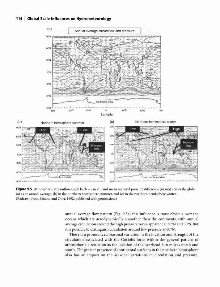
114 Global Scale Influences on Hydrometeorology
annual average flow pattern (Fig. 9.5a) this influence is most obvious over the
oceans which are aerodynamically smoother than the continents, with annual
average circulation around the high pressure zones apparent at 30°N and 30°S. But
it is possible to distinguish circulation around low pressure at 60°N.
There is a pronounced seasonal variation in the location and strength of the
circulation associated with the Coriolis force within the general pattern of
atmospheric circulation as the location of the overhead Sun moves north and
south. The greater presence of continental surfaces in the northern hemisphere
also has an impact on the seasonal variations in circulation and pressure,
18090S
60S
6060
60
40
40
40
40
−40
−100
−40
−40
−40
−40
−40−80
−40
−20
−20
0
0 0
0
00
20
20
30S
30N
60N
90N
EQ
120W 120E 18060W 60E
Latitude
Insufficient data
Annual average streamflow and pressure
0
(a)
Insufficient data
90S
60S
30S
30N
60N
90N
EQ
40
40
−40
−80
−80
60
−100100
−20
−20
−20 −40
40
0
0
0
00
0
0
0
040
40
40
100 100
Northern hemisphere winter
HighLow
Monsoonflow
(c)
0
0
0
0
000
60
80
−80
−60
−40
−20
−20
−120
60
20
20
60 60
Insufficient data
90S
60S
30S
30N
60N
90N
EQ
40
40
40
Northern hemisphere summer
High Low
Monsoonflow
(b)
Figure 9.5 Atmospheric streamflow (each barb = 2 m s−1) and mean sea level pressure difference (in mb) across the globe
(a) as an annual average, (b) in the northern hemisphere summer, and (c) in the northern hemisphere winter.
(Redrawn from Peixoto and Oort, 1992, published with permission.)
Shuttleworth_c09.indd 114Shuttleworth_c09.indd 114 11/3/2011 6:30:31 PM11/3/2011 6:30:31 PM
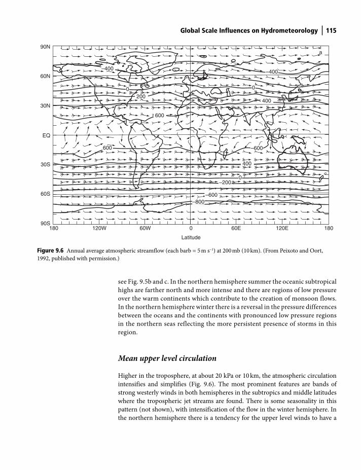
Global Scale Influences on Hydrometeorology 115
see Fig. 9.5b and c. In the northern hemisphere summer the oceanic subtropical
highs are farther north and more intense and there are regions of low pressure
over the warm continents which contribute to the creation of monsoon flows.
In the northern hemisphere winter there is a reversal in the pressure differences
between the oceans and the continents with pronounced low pressure regions
in the northern seas reflecting the more persistent presence of storms in this
region.
Mean upper level circulation
Higher in the troposphere, at about 20 kPa or 10 km, the atmospheric circulation
intensifies and simplifies (Fig. 9.6). The most prominent features are bands of
strong westerly winds in both hemispheres in the subtropics and middle latitudes
where the tropospheric jet streams are found. There is some seasonality in this
pattern (not shown), with intensification of the flow in the winter hemisphere. In
the northern hemisphere there is a tendency for the upper level winds to have a
90N
60N–400
200
600
400
400
–2000
–600
–600
600
–800
–400
a
00
30N
EQ
30S
60S
90S180 120W 60W 0
Latitude
60E 120E 180
Figure 9.6 Annual average atmospheric streamflow (each barb = 5 m s−1) at 200 mb (10 km). (From Peixoto and Oort,
1992, published with permission.)
Shuttleworth_c09.indd 115Shuttleworth_c09.indd 115 11/3/2011 6:30:32 PM11/3/2011 6:30:32 PM
116 Global Scale Influences on Hydrometeorology
wave number of two and to move toward the equator as they flow over continents,
and away from the equator as they flow over oceans. This tendency is more
pronounced in the northern hemisphere winter. Within this average flow pattern,
the jet stream is continually developing, meandering, and decaying giving relatively
less consistent lower-level winds. The jet streams have a fundamental influence on
hydrometeorological variability.
Ocean circulation
As mentioned in Chapter 1, the oceans are the principal source of ‘memory’ in the
hydroclimatic system because of their capability to store and subsequently release
large amounts of heat energy. The thermal structure of the oceans is fundamentally
different to that of the atmosphere. Energy from the Sun is captured near the ocean
surface and some warms the atmosphere from below. As a result, air nearer the
ocean surface tends to be warmer and lighter in daytime conditions, and the
atmosphere is unstable and well-mixed throughout the boundary layer as a result.
On the other hand, solar energy warms the oceans from above, so the temperature
of the water is higher nearer the surface and the surface layer of the ocean is stable.
Some mixing of energy downward does occur as a result of the turbulence caused
by surface winds but the depth to which this occurs is limited. Consequently, the
oceans are divided into a mixed layer (typically between 100 m and 1000 m deep)
which is separated from the deep ocean below by the thermocline, i.e., the steep
negative temperature gradient that gives a stable interface between these two layers
and suppresses mixing, see Fig. 9.7.
At low latitudes, solar heating is strong and fairly constant through the year, and
the stability of the thermocline is able to keep the mixed layer fairly shallow with
limited seasonality in its depth. In middle latitudes the strength of the solar heating
changes seasonally. In the hemispherical summer, the mixed layer is again fairly
shallow as at low latitudes. However, in the hemispherical winter solar heating is
less, so the distinction between the mixed layer and deep ocean is reduced; because
the temperature gradient and stability of the thermocline is therefore less, surface
winds can mix warmer surface water to greater depth.
Sea-surface temperature (SST) provides an important lower boundary
condition on the atmosphere over the ocean surfaces that cover 70% of the globe.
As discussed in Chapter 1, there is a strong coupling between oceans and
atmosphere because of the effective exchange of energy fluxes and momentum.
Since air near open water is close to saturation, the surface temperature of the
ocean defines not only the lower boundary condition for sensible heat transfer
but also for latent heat transfer. The isotherms of annual average SST run roughly
east-west across the large oceans, from greater than 29°C at the equator to almost
–2°C near the poles where the presence of salt in the ocean depresses the freezing
point, see Fig. 9.8. However, isotherms are modified near continents in response
to wind-driven currents in the upper few hundred meters of the ocean. In the
most southerly latitudes of the southern hemisphere (not shown in Fig. 9.8), the
Shuttleworth_c09.indd 116Shuttleworth_c09.indd 116 11/3/2011 6:30:33 PM11/3/2011 6:30:33 PM
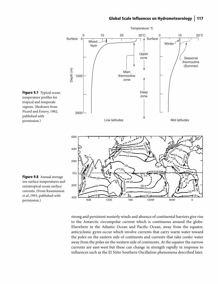
Global Scale Influences on Hydrometeorology 117
strong and persistent westerly winds and absence of continental barriers give rise
to the Antarctic circumpolar current which is continuous around the globe.
Elsewhere in the Atlantic Ocean and Pacific Ocean, away from the equator,
anticyclonic gyres occur which involve currents that carry warm water toward
the poles on the eastern side of continents and currents that take cooler water
away from the poles on the western side of continents. At the equator the narrow
currents are east-west but these can change in strength rapidly in response to
influences such as the El Niño Southern Oscillation phenomena described later.
2000
0 10 20 30�C 0 10 20�C
1000
0Surface Surface
Temperature �C
Mixedlayer
Mainthermocline
zone
Seasonalthermocline(Summer)
Low latitudes Mid latitudes
Winter
Upperzone
Deepzone
Dep
th (
m)
Figure 9.7 Typical ocean
temperature profiles for
tropical and temperate
regions. (Redrawn from
Picard and Emery, 1982,
published with
permission.)
60E40S
20S
20Agu
hius
Som
ali
(Sea
sona
lR
ever
sal)
Kuros
hio
E. A
ustr
alia
n
Per
u
Guiana
Can
ary
Bra
zil
S. Eq. S. Eq.
California
20
24
28
28
8
28
28
2726
16
12
24
24
20
2420
26
26
27
16 16
2420
1612
86
29
16
20N
40N
60N
EQ
60W 0120E 120W180
Ben
guel
a
Gul
f Stre
am
Figure 9.8 Annual average
sea-surface temperatures and
extratropical ocean surface
currents. (From Rassmusson
et al.,1993, published with
permission.)
Shuttleworth_c09.indd 117Shuttleworth_c09.indd 117 11/3/2011 6:30:33 PM11/3/2011 6:30:33 PM
118 Global Scale Influences on Hydrometeorology
In addition to the wind-driven surface currents, the thermohaline circulation is
caused by changes in density associated with the temperature and salinity of the
sea water. This originates at the poles as vertical flow that sinks to the middle
ocean or lower where it becomes horizontal. It originates as a result of density
increases likely due in part to direct cooling, but also as a result of increased salin-
ity occurring when sea water freezes and ejects additional salt into nearby saline
water. Although the downward branches of the thermohaline circulation are
largely restricted to high latitudes, the compensating upward branches occur more
widely across the globe. The thermohaline cycle is very slow, typically 1600 years,
but there is evidence that more rapid changes occur at time periods of decades
with an associated influence on climate at this time scale.
Oceanic influences on continental hydroclimate
Monsoon flow
The seasonal change in near-surface air temperature is markedly different between
oceanic and continental surfaces. Oceans have a large heat capacity and efficient cou-
pling with the atmosphere and this has the effect of moderating the seasonal cycle in
the temperature of the overlying air. The heat capacity of land surfaces is less so the
seasonal cycle can be much larger. Figure 9.9 shows isotherms of the difference
between the near-surface air temperature in January relative to that in July. Although
there are reductions of around 30°C in air temperature over the Arctic Ocean, else-
where changes in near-surface air temperature over oceans are on the order of 5–10°C.
However, the mid-continental reduction in near-surface air temperature from July to
January is more typically on the order of 40–50°C. Notice that the penetration of
maritime air into the European continent is greater than it is into the North American
continent presumably because there is less topographic obstruction to onshore flow
and the seasonal difference in near-surface air temperature is less as a result.
One important consequence of the substantial difference in temperature
between summer and winter over land surfaces relative to that over adjacent ocean
is the occurrence of monsoon air flow in the tropics. The largest monsoon system
is the Asian-Australian monsoon system (Fig. 9.10) which, recognizing the popu-
lation distribution of the world, is arguably therefore the hydroclimate phenome-
non that has most impact on humankind. In the northern hemisphere winter
season, there is a low level flow of dry, cool air from cold continent to the warmer
ocean and precipitation over the land is low. However, during the northern hemi-
sphere summer season the direction of flow is reversed, and warm, moist air flows
from the ocean over the warm land where the resulting upward motion of the
heated air produces heavy precipitation during the monsoon season. Monsoonal
flows of a broadly similar nature occur elsewhere in West Africa and in the North
American Monsoon System (NAMS), the latter being responsible for much of the
summer rain falling in northern Mexico and the southwestern USA.
Shuttleworth_c09.indd 118Shuttleworth_c09.indd 118 11/3/2011 6:30:33 PM11/3/2011 6:30:33 PM
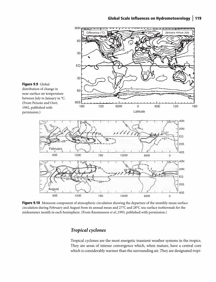
Global Scale Influences on Hydrometeorology 119
Tropical cyclones
Tropical cyclones are the most energetic transient weather systems in the tropics.
They are areas of intense convergence which, when mature, have a central core
which is considerably warmer than the surrounding air. They are designated tropi-
Figure 9.9 Global
distribution of change in
near-surface air temperature
between July to January in °C.
(From Peixoto and Oort,
1992, published with
permission.)
180 180120 12060W
20
−20−20−10
10
00
15
−10−20
−30
−40
−20−30
−30
−40
−50
−5
5
−5
10
1010
5
5
55
5
90S
60
30
30
60
90NDifference (�C) January minus July
EQ
60E
Latitude
0
60E
28
28 28
27
27
27
28
28
28
28
27
February
August
120E 120W 60W
40N
20N
20S
40S
EQ
40N
20N
20S
40S
EQ
0180
60E 120E 120W 60W 0180
Figure 9.10 Monsoon component of atmospheric circulation showing the departure of the monthly mean surface
circulation during February and August from its annual mean and 27°C and 28°C sea-surface isothermals for the
midsummer month in each hemisphere. (From Rassmusson et al.,1993, published with permission.)
Shuttleworth_c09.indd 119Shuttleworth_c09.indd 119 11/3/2011 6:30:33 PM11/3/2011 6:30:33 PM
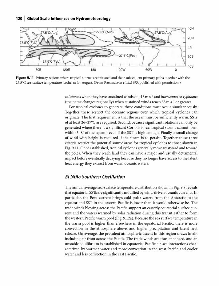
120 Global Scale Influences on Hydrometeorology
cal storms when they have sustained winds of ∼18 m s−1 and hurricanes or typhoons
(the name changes regionally) when sustained winds reach 33 m s−1 or greater.
For tropical cyclones to generate, three conditions must occur simultaneously.
Together these restrict the oceanic regions over which tropical cyclones can
originate. The first requirement is that the ocean must be sufficiently warm: SSTs
of at least 26–27°C are required. Second, because significant rotations can only be
generated where there is a significant Coriolis force, tropical storms cannot form
within 5–8° of the equator even if the SST is high enough. Finally, a small change
of wind with height is required if the storm is to persist. Together these three
criteria restrict the potential source areas for tropical cyclones to those shown in
Fig. 9.11. Once established, tropical cyclones generally move westward and toward
the poles. When they reach land they can have a major and usually detrimental
impact before eventually decaying because they no longer have access to the latent
heat energy they extract from warm oceanic waters.
El Niño Southern Oscillation
The annual average sea-surface temperature distribution shown in Fig. 9.8 reveals
that equatorial SSTs are significantly modified by wind-driven oceanic currents. In
particular, the Peru current brings cold polar waters from the Antarctic to the
equator and SST in the eastern Pacific is lower than it would otherwise be. The
trade winds blowing across the Pacific support an easterly equatorial surface cur-
rent and the waters warmed by solar radiation during this transit gather to form
the western Pacific warm pool (Fig. 9.12a). Because the sea surface temperature in
the warm pool is higher than elsewhere in the equatorial Pacific, there is more
convection in the atmosphere above, and higher precipitation and latent heat
release. On average, the prevalent atmospheric ascent in this region draws in air,
including air from across the Pacific. The trade winds are thus enhanced, and an
unstable equilibrium is established in equatorial Pacific air-sea interactions char-
acterized by warmer water and more convection in the west Pacific and cooler
water and less convection in the east Pacific.
60E 120E
27.5�C(Feb)
27.5�C(Feb)
27.5�C(Feb)
27.5�C(Aug) 27.5�C(Aug) 27.5�C(Aug)
120W 60W
40N
40S
20N
20S
EQ
0180
Figure 9.11 Primary regions where tropical storms are initiated and their subsequent primary paths together with the
27.5°C sea-surface temperature isotherm for August. (From Rassmusson et al.,1993, published with permission.)
Shuttleworth_c09.indd 120Shuttleworth_c09.indd 120 11/3/2011 6:30:34 PM11/3/2011 6:30:34 PM
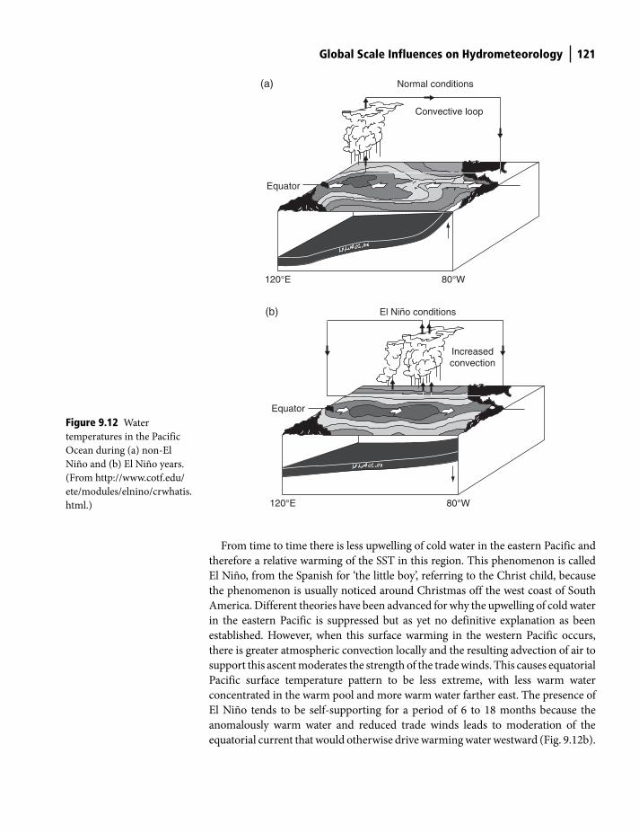
Global Scale Influences on Hydrometeorology 121
From time to time there is less upwelling of cold water in the eastern Pacific and
therefore a relative warming of the SST in this region. This phenomenon is called
El Niño, from the Spanish for ‘the little boy’, referring to the Christ child, because
the phenomenon is usually noticed around Christmas off the west coast of South
America. Different theories have been advanced for why the upwelling of cold water
in the eastern Pacific is suppressed but as yet no definitive explanation as been
established. However, when this surface warming in the western Pacific occurs,
there is greater atmospheric convection locally and the resulting advection of air to
support this ascent moderates the strength of the trade winds. This causes equatorial
Pacific surface temperature pattern to be less extreme, with less warm water
concentrated in the warm pool and more warm water farther east. The presence of
El Niño tends to be self-supporting for a period of 6 to 18 months because the
anomalously warm water and reduced trade winds leads to moderation of the
equatorial current that would otherwise drive warming water westward (Fig. 9.12b).
Normal conditions
El Niño conditions
Increasedconvection
Convective loop
120°E
Equator
80°W
120°E
Equator
(b)
(a)
80°W
Figure 9.12 Water
temperatures in the Pacific
Ocean during (a) non-El
Niño and (b) El Niño years.
(From http://www.cotf.edu/
ete/modules/elnino/crwhatis.
html.)
Shuttleworth_c09.indd 121Shuttleworth_c09.indd 121 11/3/2011 6:30:35 PM11/3/2011 6:30:35 PM
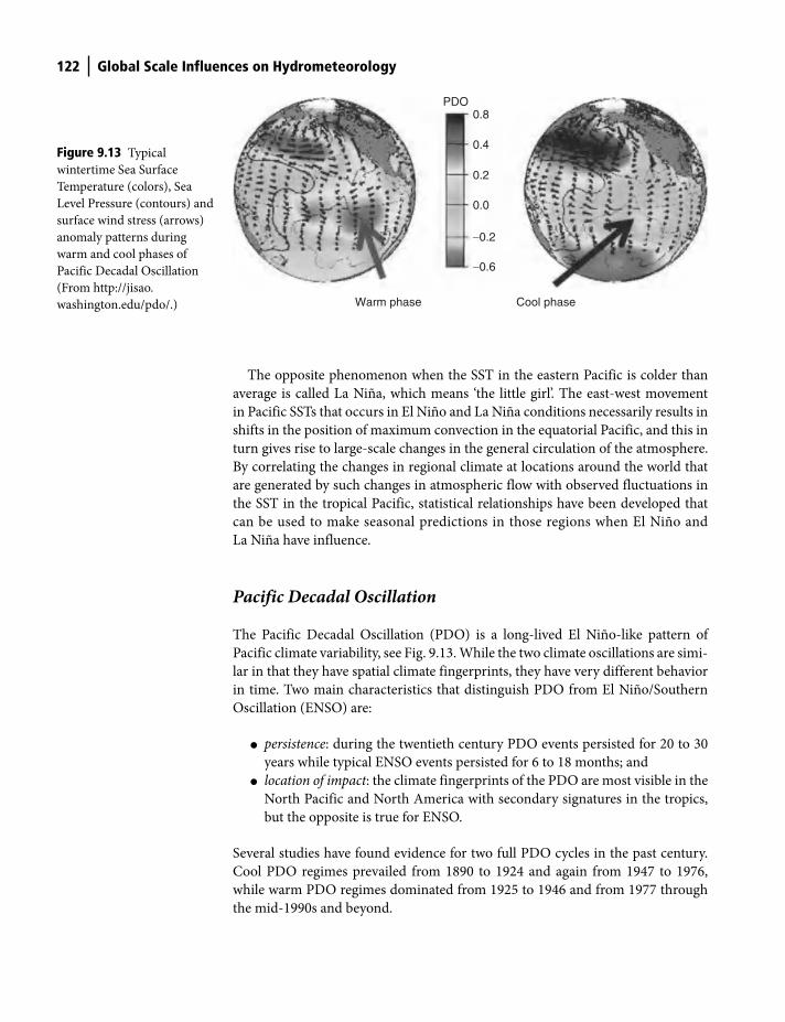
122 Global Scale Influences on Hydrometeorology
The opposite phenomenon when the SST in the eastern Pacific is colder than
average is called La Niña, which means ‘the little girl’. The east-west movement
in Pacific SSTs that occurs in El Niño and La Niña conditions necessarily results in
shifts in the position of maximum convection in the equatorial Pacific, and this in
turn gives rise to large-scale changes in the general circulation of the atmosphere.
By correlating the changes in regional climate at locations around the world that
are generated by such changes in atmospheric flow with observed fluctuations in
the SST in the tropical Pacific, statistical relationships have been developed that
can be used to make seasonal predictions in those regions when El Niño and
La Niña have influence.
Pacific Decadal Oscillation
The Pacific Decadal Oscillation (PDO) is a long-lived El Niño-like pattern of
Pacific climate variability, see Fig. 9.13. While the two climate oscillations are simi-
lar in that they have spatial climate fingerprints, they have very different behavior
in time. Two main characteristics that distinguish PDO from El Niño/Southern
Oscillation (ENSO) are:
● persistence: during the twentieth century PDO events persisted for 20 to 30
years while typical ENSO events persisted for 6 to 18 months; and
● location of impact: the climate fingerprints of the PDO are most visible in the
North Pacific and North America with secondary signatures in the tropics,
but the opposite is true for ENSO.
Several studies have found evidence for two full PDO cycles in the past century.
Cool PDO regimes prevailed from 1890 to 1924 and again from 1947 to 1976,
while warm PDO regimes dominated from 1925 to 1946 and from 1977 through
the mid-1990s and beyond.
−0.6
−0.2
0.0
0.2
0.4
0.8PDO
Warm phase Cool phase
Figure 9.13 Typical
wintertime Sea Surface
Temperature (colors), Sea
Level Pressure (contours) and
surface wind stress (arrows)
anomaly patterns during
warm and cool phases of
Pacific Decadal Oscillation
(From http://jisao.
washington.edu/pdo/.)
Shuttleworth_c09.indd 122Shuttleworth_c09.indd 122 11/3/2011 6:30:35 PM11/3/2011 6:30:35 PM
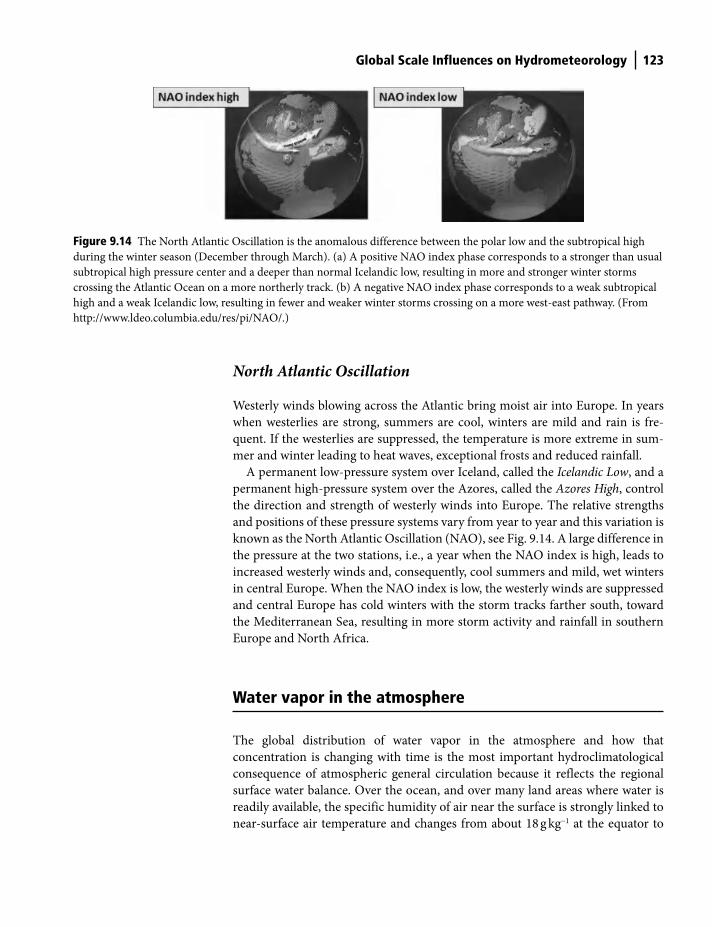
Global Scale Influences on Hydrometeorology 123
North Atlantic Oscillation
Westerly winds blowing across the Atlantic bring moist air into Europe. In years
when westerlies are strong, summers are cool, winters are mild and rain is fre-
quent. If the westerlies are suppressed, the temperature is more extreme in sum-
mer and winter leading to heat waves, exceptional frosts and reduced rainfall.
A permanent low-pressure system over Iceland, called the Icelandic Low, and a
permanent high-pressure system over the Azores, called the Azores High, control
the direction and strength of westerly winds into Europe. The relative strengths
and positions of these pressure systems vary from year to year and this variation is
known as the North Atlantic Oscillation (NAO), see Fig. 9.14. A large difference in
the pressure at the two stations, i.e., a year when the NAO index is high, leads to
increased westerly winds and, consequently, cool summers and mild, wet winters
in central Europe. When the NAO index is low, the westerly winds are suppressed
and central Europe has cold winters with the storm tracks farther south, toward
the Mediterranean Sea, resulting in more storm activity and rainfall in southern
Europe and North Africa.
Water vapor in the atmosphere
The global distribution of water vapor in the atmosphere and how that
concentration is changing with time is the most important hydroclimatological
consequence of atmospheric general circulation because it reflects the regional
surface water balance. Over the ocean, and over many land areas where water is
readily available, the specific humidity of air near the surface is strongly linked to
near-surface air temperature and changes from about 18 g kg−1 at the equator to
Figure 9.14 The North Atlantic Oscillation is the anomalous difference between the polar low and the subtropical high
during the winter season (December through March). (a) A positive NAO index phase corresponds to a stronger than usual
subtropical high pressure center and a deeper than normal Icelandic low, resulting in more and stronger winter storms
crossing the Atlantic Ocean on a more northerly track. (b) A negative NAO index phase corresponds to a weak subtropical
high and a weak Icelandic low, resulting in fewer and weaker winter storms crossing on a more west-east pathway. (From
http://www.ldeo.columbia.edu/res/pi/NAO/.)
Shuttleworth_c09.indd 123Shuttleworth_c09.indd 123 11/3/2011 6:30:36 PM11/3/2011 6:30:36 PM
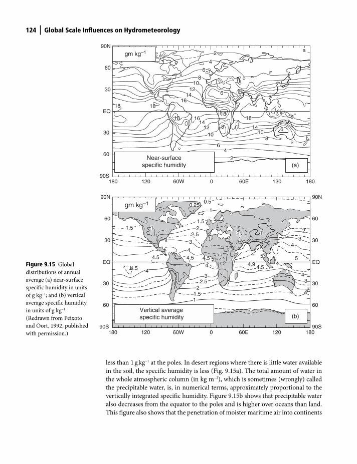
124 Global Scale Influences on Hydrometeorology
less than 1 g kg−1 at the poles. In desert regions where there is little water available
in the soil, the specific humidity is less (Fig. 9.15a). The total amount of water in
the whole atmospheric column (in kg m−2), which is sometimes (wrongly) called
the precipitable water, is, in numerical terms, approximately proportional to the
vertically integrated specific humidity. Figure 9.15b shows that precipitable water
also decreases from the equator to the poles and is higher over oceans than land.
This figure also shows that the penetration of moister maritime air into continents
90N
60
a
(a)
30
EQ
30
60
90S180 120 60W 0 60E 120 180
90N
60
30
EQ
30
60
90S
90N
60
30
EQ
30
60
90S180 120 60W 0 60E 120 180
gm kg–1
gm kg–1
Near-surfacespecific humidity
18
10
5 54.9
4.5
(b)
4.5
Vertical averagespecific humidity
11.5
22.5
3
44.54.5
4
3
4
1.52.5
21.5
4.5
1
0.50.25
1
12 11
43
2
43
5
2
46
1012
1416
1614
12
8
6
6
6
4
2
1818
18
8
18
1410
8
Figure 9.15 Global
distributions of annual
average (a) near-surface
specific humidity in units
of g kg−1; and (b) vertical
average specific humidity
in units of g kg−1.
(Redrawn from Peixoto
and Oort, 1992, published
with permission.)
Shuttleworth_c09.indd 124Shuttleworth_c09.indd 124 11/3/2011 6:30:36 PM11/3/2011 6:30:36 PM
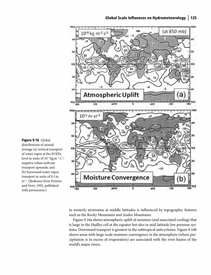
Global Scale Influences on Hydrometeorology 125
in westerly airstreams at middle latitudes is influenced by topographic features
such as the Rocky Mountains and Andes Mountains.
Figure 9.16a shows atmospheric uplift of moisture (and associated cooling) that
is large in the Hadley cell at the equator but also in mid-latitude low pressure sys-
tems. Downward transport is greatest in the subtropical anticyclones. Figure 9.16b
shows areas with large-scale moisture convergence in the atmosphere (where pre-
cipitation is in excess of evaporation) are associated with the river basins of the
world’s major rivers.
Figure 9.16 Global
distributions of annual
average (a) vertical transport
of water vapor at the 85 KPa
level in units of 10−6 kg m−2 s−1,
negative values indicate
transport upwards; and
(b) horizontal water vapor
transport in units of 0.1 m
yr−1. (Redrawn from Peixoto
and Oort, 1992, published
with permission.)
Shuttleworth_c09.indd 125Shuttleworth_c09.indd 125 11/3/2011 6:30:36 PM11/3/2011 6:30:36 PM
126 Global Scale Influences on Hydrometeorology
Important points in this chapter
● Influences on atmospheric circulation: are in three general classes:
— Planetary interrelationship, primarily:
Solar energy input (solar radiation is greater at the equator than the poles)
Seasonal perturbations (latitude of maximum solar radiation changes
with season)
Daily perturbations (the daily cycle in solar radiation changes with season)
— Persistent perturbations, primarily:
Ocean versus continent (energy return to the atmosphere differs with
surface)
Continental topography (high relief can interfere with tropospheric flow)
— Temporary perturbations, primarily:
Oceanic circulation (temporary fluctuations in SST alter atmospheric flows)
Atmospheric content (changing air content alters atmospheric radiation
transfer)
Land cover (large-scale land-cover change alters surface energy balance)
● Latitudinal radiation imbalance: atmospheric and oceanic circulation must
occur to redress the imbalance between the strong latitudinal variation in
incoming solar radiation and the weaker latitudinal variation in outgoing
longwave radiation loss.
● Lower atmosphere circulation— Latitudinal bands of pressure and wind: on average, pressure is low at the
equator with southeasterly (northeasterly) trade winds north (south) of
the equator; there is high pressure and less wind at 30°N and 30°S, but
stronger westerly winds at 60°N and 60°S.
— Hadley Circulation: there is a strong, single summer Hadley cell with
rising air located at the shifting thermal equator with falling air in the
winter hemisphere.
— Mean low-level circulation: Coriolis force gives clockwise (counterclock-
wise) circulation around high (low) pressure in the northern hemisphere
most noticeable over oceans around high pressure at 30°N and 30°S. The
circulation is reversed in the southern hemisphere. There is a seasonal
shift in the circulation pattern as the thermal equator moves north-south
that is different between hemispheres because the northern hemisphere
has a larger land area.
— Mean upper-level circulation: at ∼10 km atmospheric circulation intensi-
fies with strong westerly winds in both hemispheres in the subtropics and
middle latitudes where the tropospheric jet streams continually develop,
meander and decay giving less consistent lower-level winds and hydro-
meteorological variability.
● Ocean circulation— Thermal structure: oceans have a (∼100–1000 m deep) mixed layer
separated from the deep ocean by the thermocline, a steep negative
temperature gradient.
Shuttleworth_c09.indd 126Shuttleworth_c09.indd 126 11/3/2011 6:30:37 PM11/3/2011 6:30:37 PM
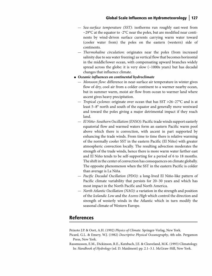
Global Scale Influences on Hydrometeorology 127
— Sea-surface temperature (SST): isotherms run roughly east-west from
∼29°C at the equator to -2°C near the poles, but are modified near conti-
nents by wind-driven surface currents carrying warm water toward
(cooler water from) the poles on the eastern (western) side of
continents.
— Thermohaline circulation: originates near the poles (from increased
salinity due to sea water freezing) as vertical flow that becomes horizontal
in the middle/lower ocean, with compensating upward branches widely
spread across the globe: it is very slow (∼1000s years) but has decadal
changes that influence climate.
● Oceanic influences on continental hydroclimate— Monsoon flow: difference in near-surface air temperature in winter gives
flow of dry, cool air from a colder continent to a warmer nearby ocean,
but in summer warm, moist air flow from ocean to warmer land where
ascent gives heavy precipitation.
— Tropical cyclones: originate over ocean that has SST >26–27°C and is at
least 5–8° north and south of the equator and generally move westward
and toward the poles giving a major detrimental impact if they reach
land.
— El Niño–Southern Oscillation (ENSO): Pacific trade winds support easterly
equatorial flow and warmed waters form an eastern Pacific warm pool
above which there is convection, with ascent in part supported by
enhancing the trade winds. From time to time there is relative warming
of the normally cooler SST in the eastern Pacific (El Niño) with greater
atmospheric convection locally. The resulting advection moderates the
strength of the trade winds, hence there is more warm water farther east
and El Niño tends to be self-supporting for a period of 6 to 18 months.
The shift in the center of convection has consequences on climate globally.
The opposite phenomenon when the SST in the eastern Pacific is colder
than average is La Niña.
— Pacific Decadal Oscillation (PDO): a long-lived El Niño-like pattern of
Pacific climate variability that persists for 20–30 years and which has
most impact in the North Pacific and North America.
— North Atlantic Oscillation (NAO): a variation in the strength and position
of the Icelandic Low and the Azores High which control the direction and
strength of westerly winds in the Atlantic which in turn modify the
seasonal climate of Western Europe.
References
Peixoto J.P. & Oort, A.H. (1992) Physics of Climate. Springer-Verlag, New York.
Picard, G.L. & Emery, W.J. (1982) Descriptive Physical Oceanography, 4th edn. Pergamon
Press, New York.
Rassmusson, E.M., Dickinson, R.E., Kutzbach, J.E. & Cleaveland, M.K. (1993) Climatology.
In: Handbook of Hydrology (ed. D. Maidment) pp. 2.1–3.1. McGraw-Hill, New York.
Shuttleworth_c09.indd 127Shuttleworth_c09.indd 127 11/3/2011 6:30:37 PM11/3/2011 6:30:37 PM
Introduction
On average, about 60% of the Earth is cloud-covered. Clouds are extremely
important in hydrometeorology because when they move in the atmosphere they
transport substantial amounts of water from one location to another. If present,
they also have a major impact on the absorption of solar radiation and modify the
surface energy balance and thereby the input of water and energy into the
atmosphere from below. Tall cumulus and stratocumulus clouds tend to shade and
inhibit solar radiation reaching the ground, but high altitude cirrus cloud tends to
blanket and inhibit the loss of longwave radiation. In seeking to predict climate
change, one of the biggest challenges is to predict how any additional water
evaporated into the atmosphere will be expressed in terms of modified cloud
cover – will that cloud reduce solar radiation input or increase the retention of
outgoing longwave radiation?
Three things are required for clouds to form. One is the presence of moisture
in the air in sufficient quantity to result in cloud if the air is cooled. This is often
the limiting constraint on cloud formation in arid and semi-arid regions such as
the southwestern US and northern Mexico. It is difficult to condense water from
air unless there is something for the water to condense on to, so a second
possible constraint on cloud formation is a lack of cloud condensation nuclei
(CCN), i.e., entities in the atmosphere around which condensation can begin.
The third important need for cloud development is a mechanism by means of
which air can be cooled sufficiently to allow condensation of water vapor. In
practice, the cooling required is usually associated with atmospheric movement,
as discussed next.
10 Formation of Clouds
Terrestrial Hydrometeorology, First Edition. W. James Shuttleworth.
© 2012 John Wiley & Sons, Ltd. Published 2012 by John Wiley & Sons, Ltd.
Shuttleworth_c10.indd 128Shuttleworth_c10.indd 128 11/3/2011 7:06:54 PM11/3/2011 7:06:54 PM
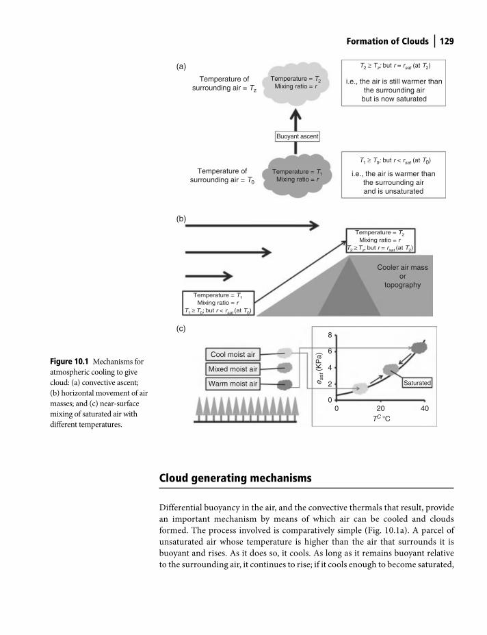
Formation of Clouds 129
Cloud generating mechanisms
Differential buoyancy in the air, and the convective thermals that result, provide
an important mechanism by means of which air can be cooled and clouds
formed. The process involved is comparatively simple (Fig. 10.1a). A parcel of
unsaturated air whose temperature is higher than the air that surrounds it is
buoyant and rises. As it does so, it cools. As long as it remains buoyant relative
to the surrounding air, it continues to rise; if it cools enough to become saturated,
Figure 10.1 Mechanisms for
atmospheric cooling to give
cloud: (a) convective ascent;
(b) horizontal movement of air
masses; and (c) near-surface
mixing of saturated air with
different temperatures.
Temperature = T2Mixing ratio = r
T2 ≥ Tz; but r = rsat (at T2)
(b)
Cooler air massor
topographyTemperature = T1
Mixing ratio = rT1 ≥ T0; but r < rsat (at T0)
Temperature ofsurrounding air = T0
Temperature ofsurrounding air = Tz
Temperature = T2Mixing ratio = r
Temperature = T1Mixing ratio = r
T1 ≥ T0; but r < rsat (at T0)
T2 ≥ Tz; but r = rsat (at T2)
i.e., the air is warmer thanthe surrounding airand is unsaturated
i.e., the air is still warmer thanthe surrounding air
but is now saturated
(a)
Buoyant ascent
(c)
Cool moist air
Mixed moist air
Warm moist air Saturated
TC �C0
0
2esat (
KP
a)
4
6
8
20 40
Shuttleworth_c10.indd 129Shuttleworth_c10.indd 129 11/3/2011 7:06:55 PM11/3/2011 7:06:55 PM
130 Formation of Clouds
cloud formation begins. Once cloud formation is underway and water vapor is
being converted to liquid water or ice, the latent heat so released further
increases the temperature of the parcel helping it to remain buoyant and thus
aiding further ascent and cooling. The cloud created in this way is called
convective cloud.
A second important way that vertical movement and associated cooling can
give rise to condensation and cloud is as a result of large-scale atmospheric
movement (Fig. 10.1b). Moving masses of air may have different temperatures and
different buoyancy. Thus, a more buoyant warm air mass moving horizontally
may, for example, impinge on and ‘float’ over a cooler air mass, or a less buoyant
cold air mass moving horizontally may impinge on a warmer air mass and ‘sink’
beneath it, pushing it upward. Thirdly, air moving horizontally may sometimes
come up against topography and be forced upward. In these examples it is the
large-scale horizontal movement of the atmosphere that is resulting in ascent and
cooling of the air, the net result being that unsaturated air moves upward, cools
and becomes saturated to give cloud.
Another way that wisps of cloud can be formed is very different because it
doesn’t involve ascent. If two portions of air that are both close to saturation but
with different temperatures are mixed, the resulting air mixture will have the
average temperature and average water content. However, because the saturated
vapor pressure curve shown in Fig. 2.2 is not linear, the resulting water content of
the mixed air may be greater than that of saturated air at the new average
temperature. Consequently, water condenses out (Fig. 10.1c). This mechanism is
not a major source of cloud but is the reason why we see sea frets and wisps of
cloud over wet forest after rain.
These different mechanisms for atmospheric condensation result in very
different types of cloud, which are subsequently associated with different patterns
of rainfall, as follows.
● Convective cloud: Because the mechanism involved in cloud formation is
associated with strong vertical ascent over fairly small horizontal areas, the
resulting cloud can be quite tall with horizontal dimensions typically on the
order of a few hundred to a few thousand meters. Moreover, being associated
with local rapid ascent, any precipitation associated with clouds of this type
tends to be heavy and local.
● Frontal cloud: The nature of the processes involved in the formation of frontal
clouds means the resulting cloud cover tends to have wide spatial coverage,
typically over areas on the order of a few kilometers to several tens of
kilometers or greater. Being associated with gradual uplift, the associated
precipitation is often widespread and steady but is usually lighter than that
for convective clouds.
● Surface mixing: The wisps of clouds produced by mixing saturated air with
different temperatures have very limited extent and are not usually associated
with precipitation.
Shuttleworth_c10.indd 130Shuttleworth_c10.indd 130 11/3/2011 7:06:56 PM11/3/2011 7:06:56 PM

Formation of Clouds 131
Cloud condensation nuclei
There are always numerous small particles, called aerosols, suspended in the atmos-
phere. Some are important because they act as the condensation nuclei required for
cloud droplet formation. Aerosols are classified according to their size as:
● Aitken Nuclei, if they have diameter in the range 0 to 0.2 μm;
● Large Nuclei, if they have diameter in the range 0.2 to 2 μm;
● Giant Aerosols, if they have diameter greater than 2 μm.
Typically the concentration of aerosols in the troposphere is on the order of 1012
per cubic meter but it can be as high as 1014 per cubic meter downwind of pollution
sources. Higher in the atmosphere, aerosol concentration falls off to about 1010 per
cubic meter at 15 km. The concentration of aerosols falls off rapidly with the
size of the aerosols so the concentration of Aitken nuclei greatly exceeds that for
giant nuclei.
Aerosols originate in many different ways but their origin can be broadly classi-
fied according to whether they result from natural phenomena or human activity.
The main source of aerosols and the amount of aerosols these sources produce
annually are listed in Table 10.1. On average natural sources are dominant,
Table 10.1 Sources of atmospheric aerosols and estimates of
the amount of aerosols produced in tonnes per year.
Natural phenomena (tonnes per year)
Airborne Sea salt 1000Gas to particle conversion 570Windblown dust particles 500Natural forest fires 35Meteoric debris 20Volcanoes (a highly variable source) 25Total from natural sources >2150
Human activities (tonnes per year)Gas to particle conversion 275Industrial processes 56Fuel combustion (stationary sources) 44Solid waste disposal 3Transportation 3Miscellaneous 28Total from human activities ∼410
Shuttleworth_c10.indd 131Shuttleworth_c10.indd 131 11/3/2011 7:06:56 PM11/3/2011 7:06:56 PM
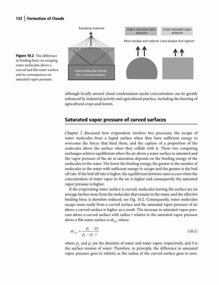
132 Formation of Clouds
although locally aerosol cloud condensation nuclei concentration can be greatly
enhanced by industrial activity and agricultural practice, including the burning of
agricultural crops and forests.
Saturated vapor pressure of curved surfaces
Chapter 2 discussed how evaporation involves two processes, the escape of
water molecules from a liquid surface when they have sufficient energy to
overcome the forces that bind them, and the capture of a proportion of the
molecules above the surface when they collide with it. These two competing
exchanges achieve equilibrium when the air above a water surface is saturated and
the vapor pressure of the air at saturation depends on the binding energy of the
molecules in the water. The lower the binding energy, the greater is the number of
molecules in the water with sufficient energy to escape and the greater is the boil
off rate. If the boil off rate is higher, the equilibrium between rates occurs when the
concentration of water vapor in the air is higher and consequently the saturated
vapor pressure is higher.
If the evaporating water surface is curved, molecules leaving the surface are on
average farther away from the molecules that remain in the water, and the effective
binding force is therefore reduced, see Fig. 10.2. Consequently, water molecules
escape more easily from a curved surface and the saturated vapor pressure of air
above a curved surface is higher as a result. The increase in saturated vapor pres-
sure above a curved surface with radius r relative to the saturated vapor pressure
above a flat water surface is desat
, where:
=−
2vsat
w v
Sder
rr r
(10.1)
where rw and r
v are the densities of water and water vapor, respectively, and S is
the surface tension of water. Therefore, in principle, the difference in saturated
vapor pressure goes to infinity as the radius of the curved surface goes to zero.
Figure 10.2 The difference
in binding force on escaping
water molecules above a
curved and flat water surface
and its consequences on
saturated vapor pressure.
Escaping molecule
More escape and capture
Higher saturated vaporpressure
Lower saturated vaporpressure
Less molecular bondsfor a curved surface
Less escape and capture
Shuttleworth_c10.indd 132Shuttleworth_c10.indd 132 11/3/2011 7:06:56 PM11/3/2011 7:06:56 PM
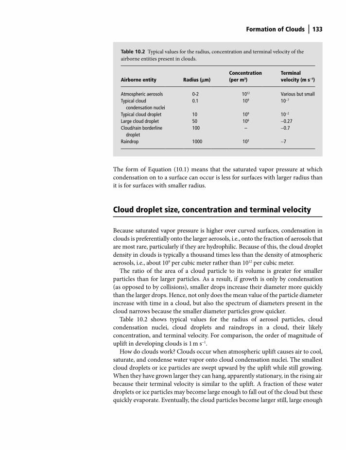
Formation of Clouds 133
The form of Equation (10.1) means that the saturated vapor pressure at which
condensation on to a surface can occur is less for surfaces with larger radius than
it is for surfaces with smaller radius.
Cloud droplet size, concentration and terminal velocity
Because saturated vapor pressure is higher over curved surfaces, condensation in
clouds is preferentially onto the larger aerosols, i.e., onto the fraction of aerosols that
are most rare, particularly if they are hydrophilic. Because of this, the cloud droplet
density in clouds is typically a thousand times less than the density of atmospheric
aerosols, i.e., about 109 per cubic meter rather than 1012 per cubic meter.
The ratio of the area of a cloud particle to its volume is greater for smaller
particles than for larger particles. As a result, if growth is only by condensation
(as opposed to by collisions), smaller drops increase their diameter more quickly
than the larger drops. Hence, not only does the mean value of the particle diameter
increase with time in a cloud, but also the spectrum of diameters present in the
cloud narrows because the smaller diameter particles grow quicker.
Table 10.2 shows typical values for the radius of aerosol particles, cloud
condensation nuclei, cloud droplets and raindrops in a cloud, their likely
concentration, and terminal velocity. For comparison, the order of magnitude of
uplift in developing clouds is 1 m s−1.
How do clouds work? Clouds occur when atmospheric uplift causes air to cool,
saturate, and condense water vapor onto cloud condensation nuclei. The smallest
cloud droplets or ice particles are swept upward by the uplift while still growing.
When they have grown larger they can hang, apparently stationary, in the rising air
because their terminal velocity is similar to the uplift. A fraction of these water
droplets or ice particles may become large enough to fall out of the cloud but these
quickly evaporate. Eventually, the cloud particles become larger still, large enough
Table 10.2 Typical values for the radius, concentration and terminal velocity of the
airborne entities present in clouds.
Airborne entity
Radius (mm) Concentration
(per m3) Terminal
velocity (m s-1)
Atmospheric aerosols 0-2 1012 Various but smallTypical cloud condensation nuclei
0.1 109 10−7
Typical cloud droplet 10 109 10−2
Large cloud droplet 50 106 ∼0.27Cloud/rain borderline droplet
100 – ∼0.7
Raindrop 1000 103 ∼7
Shuttleworth_c10.indd 133Shuttleworth_c10.indd 133 11/3/2011 7:06:58 PM11/3/2011 7:06:58 PM
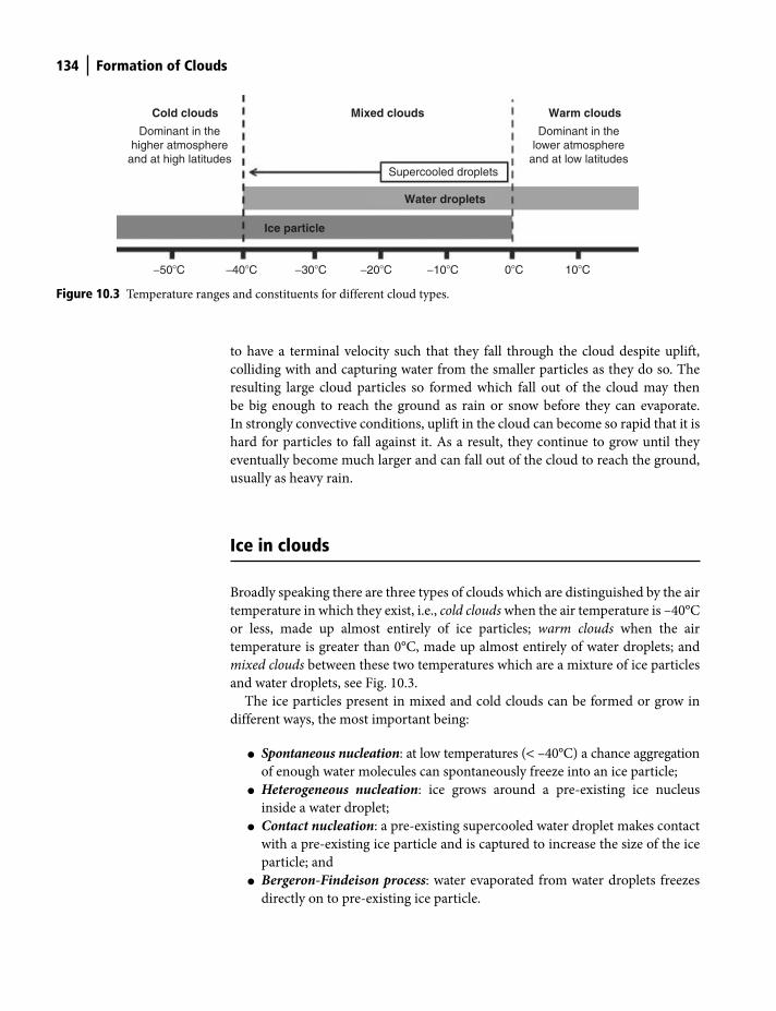
134 Formation of Clouds
to have a terminal velocity such that they fall through the cloud despite uplift,
colliding with and capturing water from the smaller particles as they do so. The
resulting large cloud particles so formed which fall out of the cloud may then
be big enough to reach the ground as rain or snow before they can evaporate.
In strongly convective conditions, uplift in the cloud can become so rapid that it is
hard for particles to fall against it. As a result, they continue to grow until they
eventually become much larger and can fall out of the cloud to reach the ground,
usually as heavy rain.
Ice in clouds
Broadly speaking there are three types of clouds which are distinguished by the air
temperature in which they exist, i.e., cold clouds when the air temperature is –40°C
or less, made up almost entirely of ice particles; warm clouds when the air
temperature is greater than 0°C, made up almost entirely of water droplets; and
mixed clouds between these two temperatures which are a mixture of ice particles
and water droplets, see Fig. 10.3.
The ice particles present in mixed and cold clouds can be formed or grow in
different ways, the most important being:
● Spontaneous nucleation: at low temperatures (< –40°C) a chance aggregation
of enough water molecules can spontaneously freeze into an ice particle;
● Heterogeneous nucleation: ice grows around a pre-existing ice nucleus
inside a water droplet;
● Contact nucleation: a pre-existing supercooled water droplet makes contact
with a pre-existing ice particle and is captured to increase the size of the ice
particle; and
● Bergeron-Findeison process: water evaporated from water droplets freezes
directly on to pre-existing ice particle.
Figure 10.3 Temperature ranges and constituents for different cloud types.
Mixed clouds
Water droplets
Ice particle
−50�C −40�C −30�C −20�C −10�C 0�C 10�C
Cold clouds
Dominant in thehigher atmosphere
and at high latitudes
Dominant in thelower atmosphere
and at low latitudesSupercooled droplets
Warm clouds
Shuttleworth_c10.indd 134Shuttleworth_c10.indd 134 11/3/2011 7:06:58 PM11/3/2011 7:06:58 PM

Formation of Clouds 135
The relative importance of these processes can influence the overall structure and
shape of the cloud and the extent and severity of any precipitation that may be
generated by them.
Cloud formation processes
Thermal convection
Whether cloud develops, and the extent and form in which it develops, depends
on the lapse rate of the advected atmosphere, i.e., on the Environmental Lapse
Rate (Ge). The Environmental Lapse Rate is the lapse rate of the incoming air mass
and so is location-specific and changes with time because it is determined by the
history of inputs and outputs to the atmosphere upstream. It might be measured
using a radiosonde attached to a balloon released into the atmosphere to provide
data for weather forecasts, including forecasts of cloud cover. The Environmental
Lapse Rate will usually include an inversion in potential temperature at the
tropopause which can stop the ascent of moist air and thus limits the vertical
extent of cloud. Near the ground the Environmental Lapse Rate is rarely equal to
(and is usually less than) the dry adiabatic lapse rate, G, this being the approximate
rate at which buoyant air cools when it ascends quickly, see Chapter 3.
The potential for cloud formation depends on the height dependent interrela-
tionship between three lapse rates, specifically:
● The environmental lapse rate, Ge – the (measured or model-calculated)
lapse rate of the air overlying the location of interest into which cloud might
be seeded.
● The dry adiabatic lapse rate, G – the rate at which air cools if is moved
upward in the atmosphere adiabatically (see Chapter 3).
● The moist adiabatic lapse rate, Gm
– the rate at which saturated air cools if it
is moved upward in the atmosphere adiabatically.
Recall that the dry adiabatic lapse rate (G = g/cp) is constant with height but that
the moist adiabatic lapse rate, Gm
, in addition to being smaller than G, increases
with temperature (see Equation 3.10). In practice, temperature decreases with
height inside a cloud, consequently the moist adiabatic lapse rate and therefore the
rate of cooling of the atmosphere increases with height.
Figure 10.4 illustrates the rate of cooling of a buoyant parcel of air (created by
surface warming) that is seeded into the atmosphere with three different
Environmental Lapse Rates which we refer to as Case 1, 2, and 3. In all three cases
the air parcel initially rises at the dry adiabatic lapse rate. In Case 1, the air is so dry
that the dry adiabatic rate intersects the environmental lapse rate before the air has
cooled enough to saturate, consequently no cloud develops. In Cases 2 and 3 the
air is initially moister. Consequently, the parcel rises and cools at the dry adiabatic
Shuttleworth_c10.indd 135Shuttleworth_c10.indd 135 11/3/2011 7:06:58 PM11/3/2011 7:06:58 PM
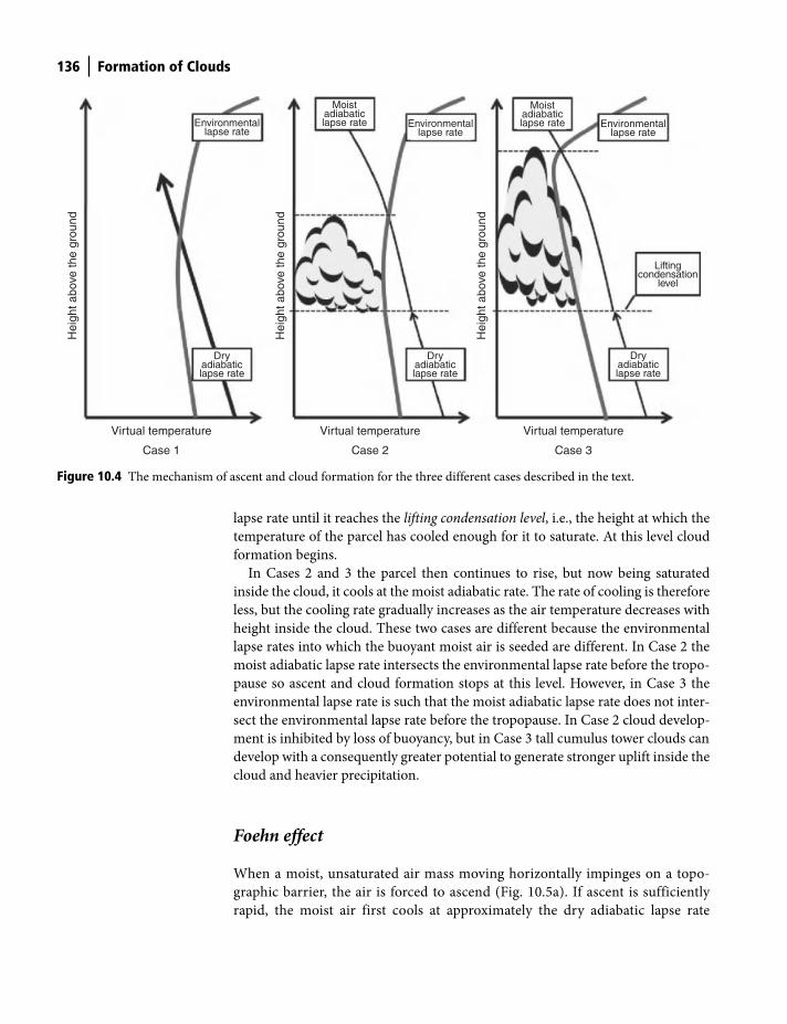
136 Formation of Clouds
lapse rate until it reaches the lifting condensation level, i.e., the height at which the
temperature of the parcel has cooled enough for it to saturate. At this level cloud
formation begins.
In Cases 2 and 3 the parcel then continues to rise, but now being saturated
inside the cloud, it cools at the moist adiabatic rate. The rate of cooling is therefore
less, but the cooling rate gradually increases as the air temperature decreases with
height inside the cloud. These two cases are different because the environmental
lapse rates into which the buoyant moist air is seeded are different. In Case 2 the
moist adiabatic lapse rate intersects the environmental lapse rate before the tropo-
pause so ascent and cloud formation stops at this level. However, in Case 3 the
environmental lapse rate is such that the moist adiabatic lapse rate does not inter-
sect the environmental lapse rate before the tropopause. In Case 2 cloud develop-
ment is inhibited by loss of buoyancy, but in Case 3 tall cumulus tower clouds can
develop with a consequently greater potential to generate stronger uplift inside the
cloud and heavier precipitation.
Foehn effect
When a moist, unsaturated air mass moving horizontally impinges on a topo-
graphic barrier, the air is forced to ascend (Fig. 10.5a). If ascent is sufficiently
rapid, the moist air first cools at approximately the dry adiabatic lapse rate
Figure 10.4 The mechanism of ascent and cloud formation for the three different cases described in the text.
Virtual temperature Virtual temperature
Hei
ght a
bove
the
grou
nd
Hei
ght a
bove
the
grou
nd
Hei
ght a
bove
the
grou
nd
Case 2
Virtual temperature
Case 3Case 1
Dryadiabaticlapse rate
Moistadiabaticlapse rate
Moistadiabaticlapse rateEnvironmental
lapse rateEnvironmental
lapse rateEnvironmental
lapse rate
Dryadiabaticlapse rate
Dryadiabaticlapse rate
Liftingcondensation
level
Shuttleworth_c10.indd 136Shuttleworth_c10.indd 136 11/3/2011 7:06:58 PM11/3/2011 7:06:58 PM
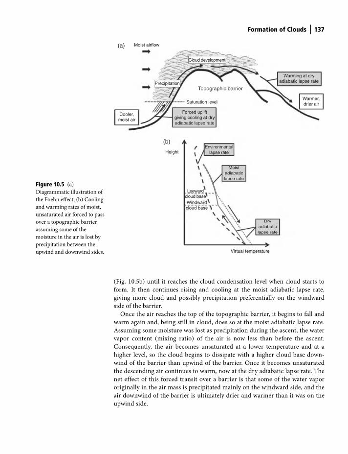
Formation of Clouds 137
(Fig. 10.5b) until it reaches the cloud condensation level when cloud starts to
form. It then continues rising and cooling at the moist adiabatic lapse rate,
giving more cloud and possibly precipitation preferentially on the windward
side of the barrier.
Once the air reaches the top of the topographic barrier, it begins to fall and
warm again and, being still in cloud, does so at the moist adiabatic lapse rate.
Assuming some moisture was lost as precipitation during the ascent, the water
vapor content (mixing ratio) of the air is now less than before the ascent.
Consequently, the air becomes unsaturated at a lower temperature and at a
higher level, so the cloud begins to dissipate with a higher cloud base down-
wind of the barrier than upwind of the barrier. Once it becomes unsaturated
the descending air continues to warm, now at the dry adiabatic lapse rate. The
net effect of this forced transit over a barrier is that some of the water vapor
originally in the air mass is precipitated mainly on the windward side, and the
air downwind of the barrier is ultimately drier and warmer than it was on the
upwind side.
Figure 10.5 (a)
Diagrammatic illustration of
the Foehn effect; (b) Cooling
and warming rates of moist,
unsaturated air forced to pass
over a topographic barrier
assuming some of the
moisture in the air is lost by
precipitation between the
upwind and downwind sides.
Moist airflow
Cloud development
Precipitation
Forced upliftgiving cooling at dryadiabatic lapse rate
Environmentallapse rate
Leewardcloud baseWindwardcloud base
Moistadiabaticlapse rate
Dry
adiabatic
lapse rate
Warmer,drier air
Warming at dryadiabatic lapse rate
Topographic barrier
Cooler,moist air
Height
Virtual temperature
Saturation level
(a)
(b)
Shuttleworth_c10.indd 137Shuttleworth_c10.indd 137 11/3/2011 7:06:59 PM11/3/2011 7:06:59 PM
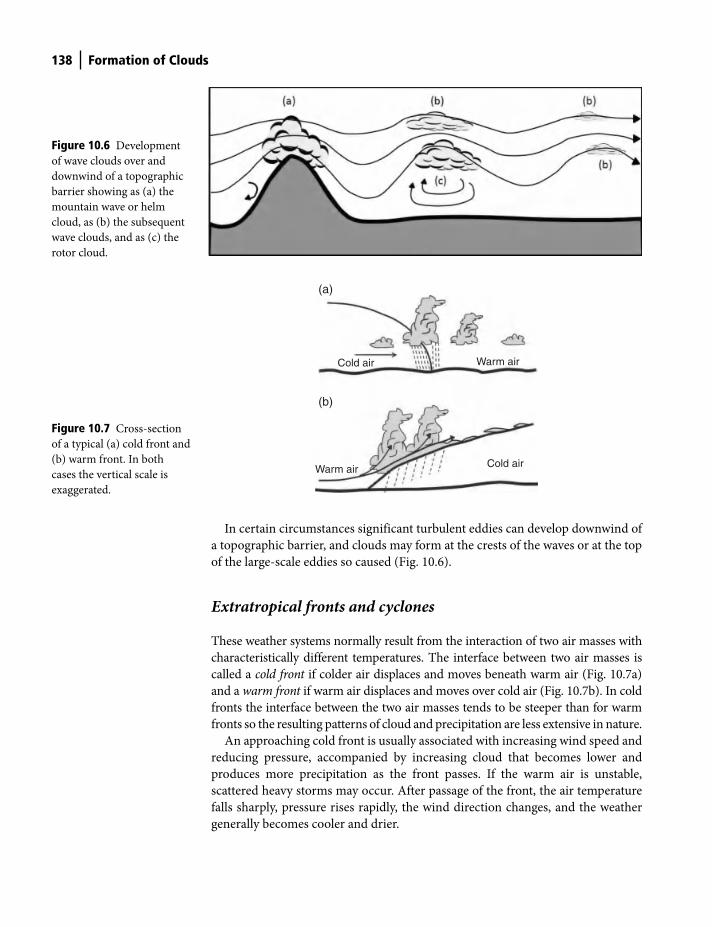
138 Formation of Clouds
In certain circumstances significant turbulent eddies can develop downwind of
a topographic barrier, and clouds may form at the crests of the waves or at the top
of the large-scale eddies so caused (Fig. 10.6).
Extratropical fronts and cyclones
These weather systems normally result from the interaction of two air masses with
characteristically different temperatures. The interface between two air masses is
called a cold front if colder air displaces and moves beneath warm air (Fig. 10.7a)
and a warm front if warm air displaces and moves over cold air (Fig. 10.7b). In cold
fronts the interface between the two air masses tends to be steeper than for warm
fronts so the resulting patterns of cloud and precipitation are less extensive in nature.
An approaching cold front is usually associated with increasing wind speed and
reducing pressure, accompanied by increasing cloud that becomes lower and
produces more precipitation as the front passes. If the warm air is unstable,
scattered heavy storms may occur. After passage of the front, the air temperature
falls sharply, pressure rises rapidly, the wind direction changes, and the weather
generally becomes cooler and drier.
Figure 10.6 Development
of wave clouds over and
downwind of a topographic
barrier showing as (a) the
mountain wave or helm
cloud, as (b) the subsequent
wave clouds, and as (c) the
rotor cloud.
Figure 10.7 Cross-section
of a typical (a) cold front and
(b) warm front. In both
cases the vertical scale is
exaggerated.
(a)
(b)
Cold air
Cold air
Warm air
Warm air
Shuttleworth_c10.indd 138Shuttleworth_c10.indd 138 11/3/2011 7:06:59 PM11/3/2011 7:06:59 PM
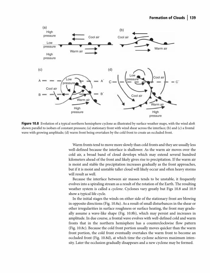
Formation of Clouds 139
Warm fronts tend to move more slowly than cold fronts and they are usually less
well-defined because the interface is shallower. As the warm air moves over the
cold air, a broad band of cloud develops which may extend several hundred
kilometers ahead of the front and likely gives rise to precipitation. If the warm air
is moist and stable the precipitation increases gradually as the front approaches,
but if it is moist and unstable taller cloud will likely occur and often heavy storms
will result as well.
Because the interface between air masses tends to be unstable, it frequently
evolves into a spiraling stream as a result of the rotation of the Earth. The resulting
weather system is called a cyclone. Cyclones vary greatly but Figs 10.8 and 10.9
show a typical life cycle.
In the initial stages the winds on either side of the stationary front are blowing
in opposite directions (Fig. 10.8a). As a result of small disturbances in the shear or
other irregularities in surface roughness or surface heating, the front may gradu-
ally assume a wave-like shape (Fig. 10.8b), which may persist and increases in
amplitude. In due course, a frontal wave evolves with well-defined cold and warm
fronts that in the northern hemisphere has a counterclockwise flow pattern
(Fig. 10.8c). Because the cold front portion usually moves quicker than the warm
front portion, the cold front eventually overtakes the warm front to become an
occluded front (Fig. 10.8d), at which time the cyclone achieves maximum inten-
sity. Later the occlusion gradually disappears and a new cyclone may be formed.
Figure 10.8 Evolution of a typical northern hemisphere cyclone as illustrated by surface weather maps, with the wind aloft
shown parallel to isobars of constant pressure; (a) stationary front with wind shear across the interface; (b) and (c) a frontal
wave with growing amplitude; (d) warm front being overtaken by the cold front to create an occluded front.
(a)High
pressure
Warm air
Cool air
Highpressure
Lowpressure
Warm air
Cool air
(b)
(c)
Warm air
Cool air
A A´
B B´
Highpressure
Lowpressure
Warm air
Cool air
Cool air
C´
Highpressure
Lowpressure
(d)
C
Shuttleworth_c10.indd 139Shuttleworth_c10.indd 139 11/3/2011 7:07:00 PM11/3/2011 7:07:00 PM
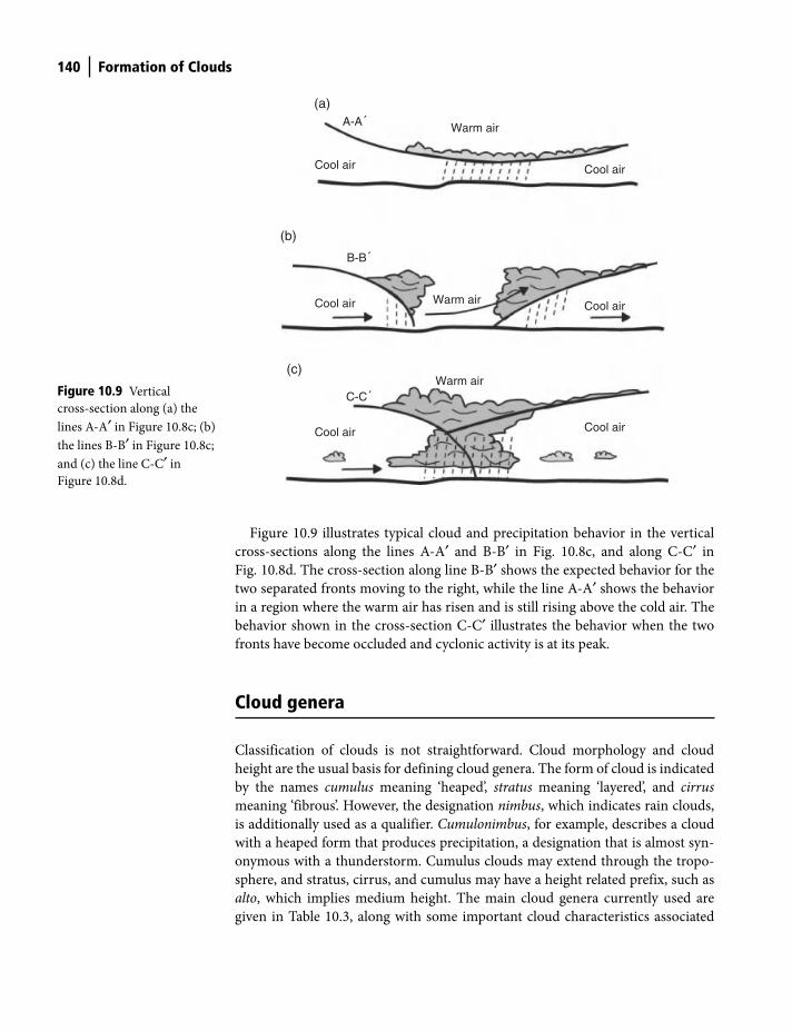
140 Formation of Clouds
Figure 10.9 illustrates typical cloud and precipitation behavior in the vertical
cross-sections along the lines A-A′ and B-B′ in Fig. 10.8c, and along C-C′ in
Fig. 10.8d. The cross-section along line B-B′ shows the expected behavior for the
two separated fronts moving to the right, while the line A-A′ shows the behavior
in a region where the warm air has risen and is still rising above the cold air. The
behavior shown in the cross-section C-C′ illustrates the behavior when the two
fronts have become occluded and cyclonic activity is at its peak.
Cloud genera
Classification of clouds is not straightforward. Cloud morphology and cloud
height are the usual basis for defining cloud genera. The form of cloud is indicated
by the names cumulus meaning ‘heaped’, stratus meaning ‘layered’, and cirrus
meaning ‘fibrous’. However, the designation nimbus, which indicates rain clouds,
is additionally used as a qualifier. Cumulonimbus, for example, describes a cloud
with a heaped form that produces precipitation, a designation that is almost syn-
onymous with a thunderstorm. Cumulus clouds may extend through the tropo-
sphere, and stratus, cirrus, and cumulus may have a height related prefix, such as
alto, which implies medium height. The main cloud genera currently used are
given in Table 10.3, along with some important cloud characteristics associated
Figure 10.9 Vertical
cross-section along (a) the
lines A-A′ in Figure 10.8c; (b)
the lines B-B′ in Figure 10.8c;
and (c) the line C-C′ in
Figure 10.8d.
Warm air
Cool airCool air
Warm air
Warm air
Cool air
Cool airCool air
Cool air
A-A´
B-B´
(a)
(b)
(c)
C-C´
Shuttleworth_c10.indd 140Shuttleworth_c10.indd 140 11/3/2011 7:07:00 PM11/3/2011 7:07:00 PM
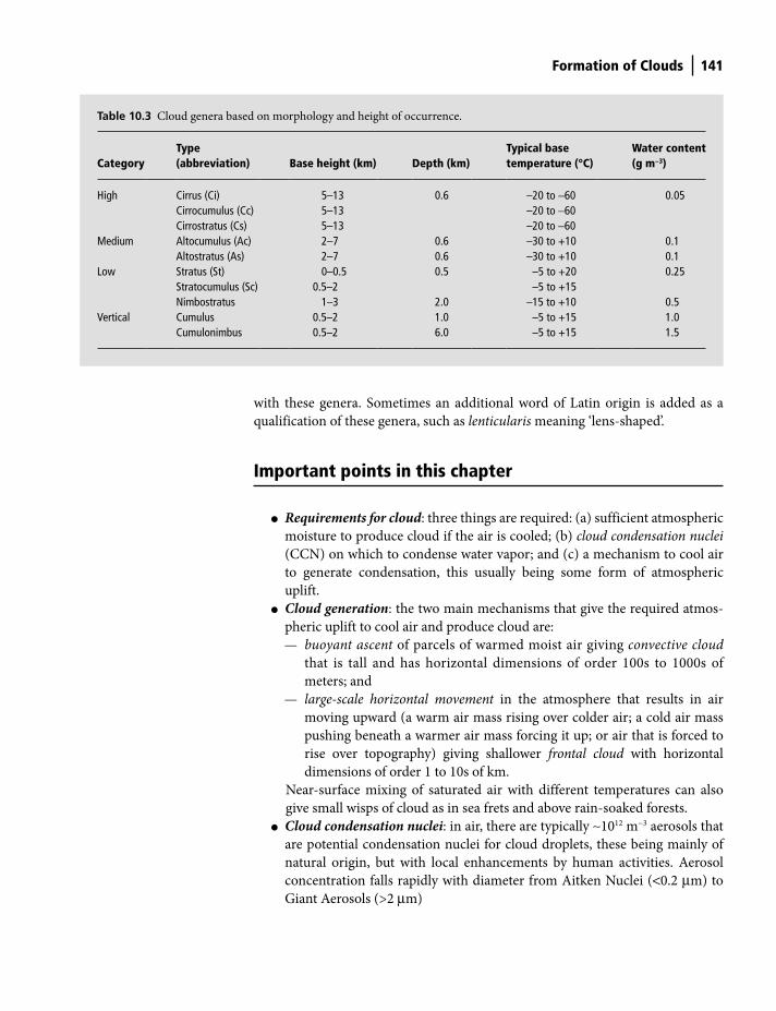
Formation of Clouds 141
with these genera. Sometimes an additional word of Latin origin is added as a
qualification of these genera, such as lenticularis meaning ‘lens-shaped’.
Important points in this chapter
● Requirements for cloud: three things are required: (a) sufficient atmospheric
moisture to produce cloud if the air is cooled; (b) cloud condensation nuclei
(CCN) on which to condense water vapor; and (c) a mechanism to cool air
to generate condensation, this usually being some form of atmospheric
uplift.
● Cloud generation: the two main mechanisms that give the required atmos-
pheric uplift to cool air and produce cloud are:
— buoyant ascent of parcels of warmed moist air giving convective cloud
that is tall and has horizontal dimensions of order 100s to 1000s of
meters; and
— large-scale horizontal movement in the atmosphere that results in air
moving upward (a warm air mass rising over colder air; a cold air mass
pushing beneath a warmer air mass forcing it up; or air that is forced to
rise over topography) giving shallower frontal cloud with horizontal
dimensions of order 1 to 10s of km.
Near-surface mixing of saturated air with different temperatures can also
give small wisps of cloud as in sea frets and above rain-soaked forests.
● Cloud condensation nuclei: in air, there are typically ∼1012 m−3 aerosols that
are potential condensation nuclei for cloud droplets, these being mainly of
natural origin, but with local enhancements by human activities. Aerosol
concentration falls rapidly with diameter from Aitken Nuclei (<0.2 μm) to
Giant Aerosols (>2 μm)
Table 10.3 Cloud genera based on morphology and height of occurrence.
Category Type (abbreviation) Base height (km) Depth (km)
Typical base temperature (°C)
Water content (g m−3)
High Cirrus (Ci) 5–13 0.6 –20 to −60 0.05Cirrocumulus (Cc) 5–13 –20 to −60Cirrostratus (Cs) 5–13 –20 to −60
Medium Altocumulus (Ac) 2–7 0.6 –30 to +10 0.1Altostratus (As) 2–7 0.6 –30 to +10 0.1
Low Stratus (St) 0–0.5 0.5 –5 to +20 0.25Stratocumulus (Sc) 0.5–2 –5 to +15Nimbostratus 1–3 2.0 –15 to +10 0.5
Vertical Cumulus 0.5–2 1.0 –5 to +15 1.0 Cumulonimbus 0.5–2 6.0 –5 to +15 1.5
Shuttleworth_c10.indd 141Shuttleworth_c10.indd 141 11/3/2011 7:07:01 PM11/3/2011 7:07:01 PM

142 Formation of Clouds
● Vapor pressure near curved surfaces: saturated vapor pressure above curved
surfaces is higher because water molecules can escape more readily from
them so condensation is easier onto droplets with larger radius.
● Droplet concentration: cloud droplet density is about 1000 times less than
aerosol density (∼109 m−3 versus ∼1012 m−3) because condensation is easier
onto larger radii aerosols that are much less common (see last two points).
● How do clouds work?: smaller cloud particles with lower terminal velocity
are swept upward or hang almost stationary in the atmospheric uplift in
clouds until some particles grow large enough to fall quickly through the
cloud, gathering water from smaller particles as they do so. These leave the
cloud and some may be big enough to reach the ground before evaporating.
● Cloud types: three types of cloud are distinguished by their temperature,
cold clouds (< –40°C), mixed clouds (–40°C to 0°C) and warm clouds (>0°C).
● Cloud formation: three important cloud formation mechanisms described
in the text are Thermal convection, the Froehn effect, and Extratropical fronts
and cyclones.
● Cloud genera: cumulus means ‘heaped’, stratus means ‘layered’, and cirrus
means ‘fibrous’, with nimbus indicating rain clouds used as a qualifier, and
alto and cirro respectively used as a prefix to indicate ‘medium’ and ‘high’.
Shuttleworth_c10.indd 142Shuttleworth_c10.indd 142 11/3/2011 7:07:01 PM11/3/2011 7:07:01 PM
Introduction
As discussed in the last chapter, clouds are made up of cloud droplets, ice particles,
or a mixture of the two, depending on the temperature of the cloud and therefore
on its height and location. It is very difficult for these basic constituents to reach
the ground because they are small in size and so have very low terminal velocity;
there is also often uplift in the cloud that counteracts the tendency they have to
fall. Even droplets or particles that are just large enough to fall out of the cloud are
likely to evaporate before they reach the ground, once they leave the saturated
atmosphere inside the cloud.
Moreover, cloud particles do not grow rapidly enough by simple condensation
to fall as precipitation. Some other growth mechanism is required. As discussed in
more detail below, there are two general ways cloud particles can grow more
quickly. The first is via some form of collision. The name given to growth processes
that involve collision is different depending on the phase of the cloud particles
involved. When water droplets collide with other water droplets and grow as a
result, the process is called coalescence. This can occur in both warm clouds and
mixed clouds. When ice particles grow by colliding with other ice particles, the
growth process is called aggregation. This can occur in both cold clouds and mixed
clouds. When an ice particle grows by colliding with and freezing the water from
(or riming) water droplets, the process is called accretion. This process can only
occur in mixed clouds. All of these collision processes require that there is air
motion within the cloud, but this is a common phenomenon in clouds.
A second way that ice particles grow in mixed clouds is by the Bergeron-
Findeisen process. In this process (described in greater detail later) ice particles
grow at the expense of water droplets in the cloud because there is a difference in
the saturated vapor pressure for ice and water at the same temperature. This growth
process does not necessarily require internal movement in the cloud, but it can
Formation of Precipitation11
Terrestrial Hydrometeorology, First Edition. W. James Shuttleworth.
© 2012 John Wiley & Sons, Ltd. Published 2012 by John Wiley & Sons, Ltd.
Shuttleworth_c11.indd 143Shuttleworth_c11.indd 143 11/3/2011 7:06:28 PM11/3/2011 7:06:28 PM
144 Formation of Precipitation
obviously only give growth in mixed cloud where both phases of water coexist. It is
worth noting that there are more growth processes available for mixed clouds, i.e.,
all the collision processes as well as the Bergeron-Findeisen process, and their ability
to produce precipitation is therefore greater than for warm clouds or cold clouds.
Precipitation formation in warm clouds
It is clear from the discussion above that, in clouds that ultimately produce pre-
cipitation, the growth of cloud particles is complex, and that it is particularly so for
mixed clouds. A full description of the microphysics of cloud evolution is beyond
the scope of this text. However, it is helpful to consider at least the simplest case of
droplet growth in warm clouds to provide basic insight into the complex process
of collision growth.
By definition, the air temperature in a warm cloud is above 0°C. Consequently,
warm clouds are found below the 0°C isotherm, which means they have a limited
depth at middle and high latitudes where they make only a small contribution to
precipitation. But their contribution to tropical precipitation and to warm season
precipitation can be appreciable. In warm clouds, coalescence is the only collision
mechanism available for cloud particle growth. It occurs between droplets or drops
of different size that are, therefore, falling at different rates. The larger drop falls more
quickly and collides with and potentially captures the slower moving smaller drop.
The likelihood of two water droplets colliding can be expressed in terms of an
impact parameter, y, which is equal to the distance between the geometric centers of
the two droplets (Fig. 11.1a). Collision is likely if y =0 and unlikely if y >> (R + r),
where R is the radius of the larger ‘collector’ drop and r is the radius of the smaller
drop with which the collector drop collides. However, the distinction between
whether there is or is not a collision is blurred because complications arise, some of
which are illustrated in Fig. 11.1b. The collision efficiency, E1, is defined to be the
effective area for which collision of the two cloud droplets is certain relative to the area
[π(R + r)2] for which collision would be certain in the absence of these complicating
processes. The value of E1 varies from near zero when both cloud droplets are small to
near unity when both are large (Fig. 11.2). However, not all collisions will result in the
two droplets coalescing because, having collided, they can then subsequently break
apart. So it is necessary to multiply E1 by the coalescence efficiency, E
2, which decreases
markedly for droplets of similar size, to give the collection efficiency, Ec, with which a
falling droplet will collide with and then absorb another droplet, hence Ec = (E
1E
2).
Attempts have been made to estimate E1, E
2, and E
c theoretically, but it is very difficult
to validate these theoretical estimates experimentally.
Given a (perhaps approximate) description of the collection of droplets by a
single droplet, the next step is to imagine a large droplet of radius R falling though
a field of smaller droplets that are of uniform radius r and equally distributed in
space. Assuming R >> r, it can be easily shown that the resulting rate of growth in
the radius R is given by:
Shuttleworth_c11.indd 144Shuttleworth_c11.indd 144 11/3/2011 7:06:29 PM11/3/2011 7:06:29 PM
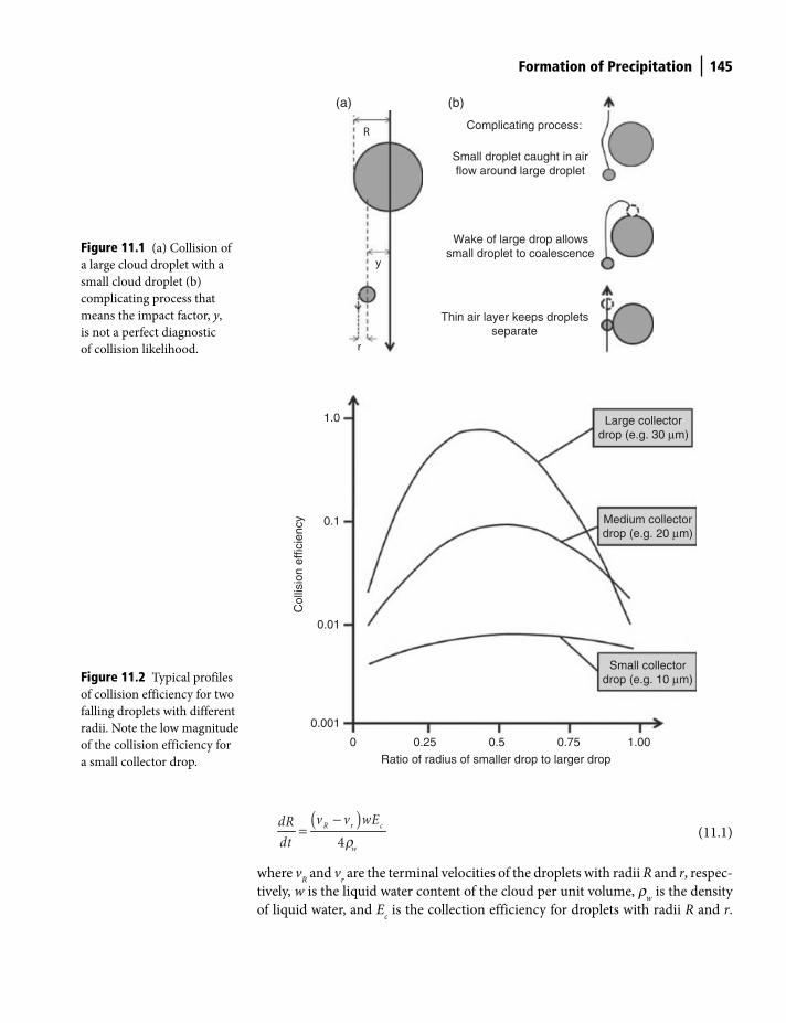
Formation of Precipitation 145
( )−=
4
R r c
w
v v wEdRdt r
(11.1)
where vR and v
r are the terminal velocities of the droplets with radii R and r, respec-
tively, w is the liquid water content of the cloud per unit volume, rw is the density
of liquid water, and Ec is the collection efficiency for droplets with radii R and r.
Figure 11.1 (a) Collision of
a large cloud droplet with a
small cloud droplet (b)
complicating process that
means the impact factor, y,
is not a perfect diagnostic
of collision likelihood.
(a)
R
y
r
Complicating process:
Thin air layer keeps dropletsseparate
Wake of large drop allowssmall droplet to coalescence
Small droplet caught in airflow around large droplet
(b)
Figure 11.2 Typical profiles
of collision efficiency for two
falling droplets with different
radii. Note the low magnitude
of the collision efficiency for
a small collector drop.
0.001
0 0.25 0.5 0.75 1.00
Medium collectordrop (e.g. 20 μm)
Large collectordrop (e.g. 30 μm)
Small collectordrop (e.g. 10 μm)
Ratio of radius of smaller drop to larger drop
Col
lisio
n ef
ficie
ncy
0.01
0.1
1.0
Shuttleworth_c11.indd 145Shuttleworth_c11.indd 145 11/3/2011 7:06:29 PM11/3/2011 7:06:29 PM
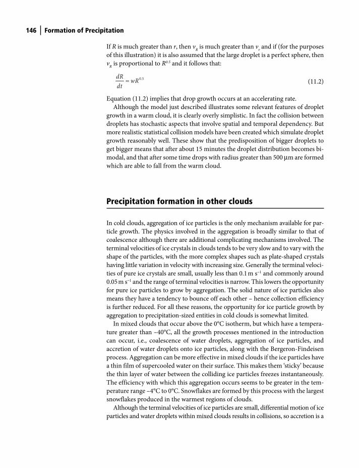
146 Formation of Precipitation
If R is much greater than r, then vR is much greater than v
r and if (for the purposes
of this illustration) it is also assumed that the large droplet is a perfect sphere, then
vR is proportional to R0.5 and it follows that:
0.5dR wRdt
≈
(11.2)
Equation (11.2) implies that drop growth occurs at an accelerating rate.
Although the model just described illustrates some relevant features of droplet
growth in a warm cloud, it is clearly overly simplistic. In fact the collision between
droplets has stochastic aspects that involve spatial and temporal dependency. But
more realistic statistical collision models have been created which simulate droplet
growth reasonably well. These show that the predisposition of bigger droplets to
get bigger means that after about 15 minutes the droplet distribution becomes bi-
modal, and that after some time drops with radius greater than 500 μm are formed
which are able to fall from the warm cloud.
Precipitation formation in other clouds
In cold clouds, aggregation of ice particles is the only mechanism available for par-
ticle growth. The physics involved in the aggregation is broadly similar to that of
coalescence although there are additional complicating mechanisms involved. The
terminal velocities of ice crystals in clouds tends to be very slow and to vary with the
shape of the particles, with the more complex shapes such as plate-shaped crystals
having little variation in velocity with increasing size. Generally the terminal veloci-
ties of pure ice crystals are small, usually less than 0.1 m s−1 and commonly around
0.05 m s−1 and the range of terminal velocities is narrow. This lowers the opportunity
for pure ice particles to grow by aggregation. The solid nature of ice particles also
means they have a tendency to bounce off each other – hence collection efficiency
is further reduced. For all these reasons, the opportunity for ice particle growth by
aggregation to precipitation-sized entities in cold clouds is somewhat limited.
In mixed clouds that occur above the 0°C isotherm, but which have a tempera-
ture greater than –40°C, all the growth processes mentioned in the introduction
can occur, i.e., coalescence of water droplets, aggregation of ice particles, and
accretion of water droplets onto ice particles, along with the Bergeron-Findeisen
process. Aggregation can be more effective in mixed clouds if the ice particles have
a thin film of supercooled water on their surface. This makes them ‘sticky’ because
the thin layer of water between the colliding ice particles freezes instantaneously.
The efficiency with which this aggregation occurs seems to be greater in the tem-
perature range –4°C to 0°C. Snowflakes are formed by this process with the largest
snowflakes produced in the warmest regions of clouds.
Although the terminal velocities of ice particles are small, differential motion of ice
particles and water droplets within mixed clouds results in collisions, so accretion is a
Shuttleworth_c11.indd 146Shuttleworth_c11.indd 146 11/3/2011 7:06:31 PM11/3/2011 7:06:31 PM
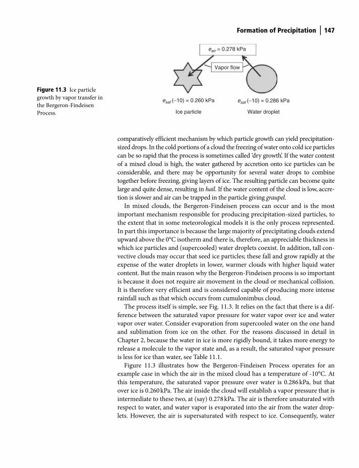
Formation of Precipitation 147
comparatively efficient mechanism by which particle growth can yield precipitation-
sized drops. In the cold portions of a cloud the freezing of water onto cold ice particles
can be so rapid that the process is sometimes called ‘dry growth’. If the water content
of a mixed cloud is high, the water gathered by accretion onto ice particles can be
considerable, and there may be opportunity for several water drops to combine
together before freezing, giving layers of ice. The resulting particle can become quite
large and quite dense, resulting in hail. If the water content of the cloud is low, accre-
tion is slower and air can be trapped in the particle giving graupel.
In mixed clouds, the Bergeron-Findeisen process can occur and is the most
important mechanism responsible for producing precipitation-sized particles, to
the extent that in some meteorological models it is the only process represented.
In part this importance is because the large majority of precipitating clouds extend
upward above the 0°C isotherm and there is, therefore, an appreciable thickness in
which ice particles and (supercooled) water droplets coexist. In addition, tall con-
vective clouds may occur that seed ice particles; these fall and grow rapidly at the
expense of the water droplets in lower, warmer clouds with higher liquid water
content. But the main reason why the Bergeron-Findeisen process is so important
is because it does not require air movement in the cloud or mechanical collision.
It is therefore very efficient and is considered capable of producing more intense
rainfall such as that which occurs from cumulonimbus cloud.
The process itself is simple, see Fig. 11.3. It relies on the fact that there is a dif-
ference between the saturated vapor pressure for water vapor over ice and water
vapor over water. Consider evaporation from supercooled water on the one hand
and sublimation from ice on the other. For the reasons discussed in detail in
Chapter 2, because the water in ice is more rigidly bound, it takes more energy to
release a molecule to the vapor state and, as a result, the saturated vapor pressure
is less for ice than water, see Table 11.1.
Figure 11.3 illustrates how the Bergeron-Findeisen Process operates for an
example case in which the air in the mixed cloud has a temperature of -10°C. At
this temperature, the saturated vapor pressure over water is 0.286 kPa, but that
over ice is 0.260 kPa. The air inside the cloud will establish a vapor pressure that is
intermediate to these two, at (say) 0.278 kPa. The air is therefore unsaturated with
respect to water, and water vapor is evaporated into the air from the water drop-
lets. However, the air is supersaturated with respect to ice. Consequently, water
Figure 11.3 Ice particle
growth by vapor transfer in
the Bergeron-Findeisen
Process. Ice particle
esat (−10) = 0.260 kPa esat (−10) = 0.286 kPa
eair = 0.278 kPa
Water droplet
Vapor flow
Shuttleworth_c11.indd 147Shuttleworth_c11.indd 147 11/3/2011 7:06:32 PM11/3/2011 7:06:32 PM
148 Formation of Precipitation
vapor is frozen out of the air and directly deposited on to the ice particles. Because
there is no physical movement of cloud particles involved, the transfer of vapor
and resulting ice particle growth can be rapid.
Which clouds produce rain?
Most clouds do not produce rain. This can be seen easily by comparing satellite
derived maps of cloud cover with simultaneous maps of precipitation intensity
derived from rainfall radar, both of which are now readily available on the Internet.
Clouds do not produce rain if they are:
● too short lived, or have not yet been in existence long enough for drops of
sufficient size to escape from the cloud and fall to the ground;
● too shallow to allow vertical motion that encourages particle growth;
● too high, which implies that they have low moisture content because they are
cold, they have limited internal vertical motion, and any precipitation gener-
ated has abundant opportunity to evaporate before reaching the ground.
Clouds that are more likely to produce precipitation have the opposite characteristics
to those given above, specifically they:
● have existed for some time, so they more likely have greater dynamical activ-
ity which includes differential vertical motion, and there has been more time
for multiple collisions to have occurred between component cloud particles;
Table 11.1 Saturated vapor pressure over water and ice as a function of temperature.
Temperature (°C) Saturated vapor pressure
over water (kPa) Saturated vapor
pressure over ice (kPa)
0 0.611 0.611–2 0.527 0.517–4 0.454 0.437–6 0.390 0.369–8 0.334 0.310–10 0.286 0.260–12 0.244 0.218–14 0.207 0.182–16 0.175 0.151–18 0.148 0.125–20 0.124 0.104
Shuttleworth_c11.indd 148Shuttleworth_c11.indd 148 11/3/2011 7:06:32 PM11/3/2011 7:06:32 PM
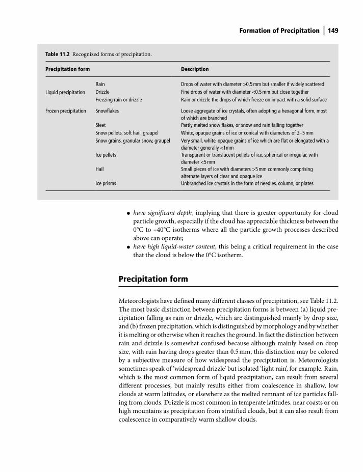
Formation of Precipitation 149
● have significant depth, implying that there is greater opportunity for cloud
particle growth, especially if the cloud has appreciable thickness between the
0°C to –40°C isotherms where all the particle growth processes described
above can operate;
● have high liquid-water content, this being a critical requirement in the case
that the cloud is below the 0°C isotherm.
Precipitation form
Meteorologists have defined many different classes of precipitation, see Table 11.2.
The most basic distinction between precipitation forms is between (a) liquid pre-
cipitation falling as rain or drizzle, which are distinguished mainly by drop size,
and (b) frozen precipitation, which is distinguished by morphology and by whether
it is melting or otherwise when it reaches the ground. In fact the distinction between
rain and drizzle is somewhat confused because although mainly based on drop
size, with rain having drops greater than 0.5 mm, this distinction may be colored
by a subjective measure of how widespread the precipitation is. Meteorologists
sometimes speak of ‘widespread drizzle’ but isolated ‘light rain’, for example. Rain,
which is the most common form of liquid precipitation, can result from several
different processes, but mainly results either from coalescence in shallow, low
clouds at warm latitudes, or elsewhere as the melted remnant of ice particles fall-
ing from clouds. Drizzle is most common in temperate latitudes, near coasts or on
high mountains as precipitation from stratified clouds, but it can also result from
coalescence in comparatively warm shallow clouds.
Table 11.2 Recognized forms of precipitation.
Precipitation form Description
Liquid precipitation
Rain Drops of water with diameter >0.5 mm but smaller if widely scatteredDrizzle Fine drops of water with diameter <0.5 mm but close togetherFreezing rain or drizzle Rain or drizzle the drops of which freeze on impact with a solid surface
Frozen precipitation Snowflakes Loose aggregate of ice crystals, often adopting a hexagonal form, most of which are branched
Sleet Partly melted snow flakes, or snow and rain falling togetherSnow pellets, soft hail, graupel White, opaque grains of ice or conical with diameters of 2–5 mmSnow grains, granular snow, graupel Very small, white, opaque grains of ice which are flat or elongated with a
diameter generally <1mmIce pellets Transparent or translucent pellets of ice, spherical or irregular, with
diameter <5 mmHail Small pieces of ice with diameters >5 mm commonly comprising
alternate layers of clear and opaque ice Ice prisms Unbranched ice crystals in the form of needles, column, or plates
Shuttleworth_c11.indd 149Shuttleworth_c11.indd 149 11/3/2011 7:06:32 PM11/3/2011 7:06:32 PM
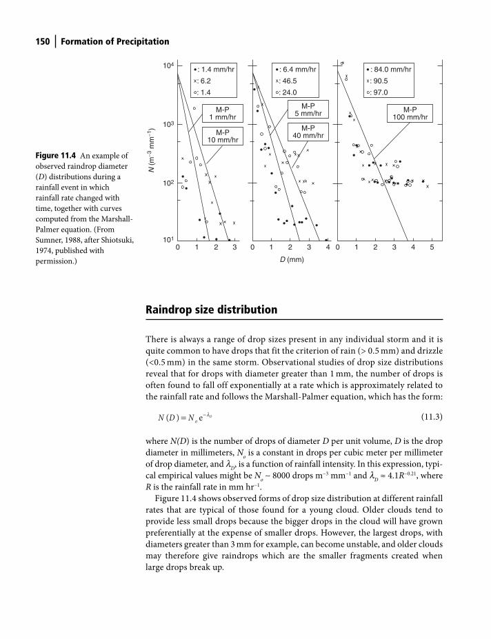
150 Formation of Precipitation
Raindrop size distribution
There is always a range of drop sizes present in any individual storm and it is
quite common to have drops that fit the criterion of rain (> 0.5 mm) and drizzle
(<0.5 mm) in the same storm. Observational studies of drop size distributions
reveal that for drops with diameter greater than 1 mm, the number of drops is
often found to fall off exponentially at a rate which is approximately related to
the rainfall rate and follows the Marshall-Palmer equation, which has the form:
−=( ) e DoN D N l
(11.3)
where N(D) is the number of drops of diameter D per unit volume, D is the drop
diameter in millimeters, No is a constant in drops per cubic meter per millimeter
of drop diameter, and lD, is a function of rainfall intensity. In this expression, typi-
cal empirical values might be No ∼ 8000 drops m−3 mm−1 and l
D ≈ 4.1R−0.21, where
R is the rainfall rate in mm hr−1.
Figure 11.4 shows observed forms of drop size distribution at different rainfall
rates that are typical of those found for a young cloud. Older clouds tend to
provide less small drops because the bigger drops in the cloud will have grown
preferentially at the expense of smaller drops. However, the largest drops, with
diameters greater than 3 mm for example, can become unstable, and older clouds
may therefore give raindrops which are the smaller fragments created when
large drops break up.
Figure 11.4 An example of
observed raindrop diameter
(D) distributions during a
rainfall event in which
rainfall rate changed with
time, together with curves
computed from the Marshall-
Palmer equation. (From
Sumner, 1988, after Shiotsuki,
1974, published with
permission.)
102
103
104
101
0
: 6.4 mm/hr
: 46.5
: 24.0
: 84.0 mm/hr
: 90.5
: 97.0
: 1.4 mm/hr
: 6.2
: 1.4
N (
m−3
mm
−1)
1 2 3 0 1 2 3 4 0 1 2 3 4 5
M-P40 mm/hr
M-P100 mm/hr
D (mm)
M-P10 mm/hr
M-P5 mm/hrM-P
1 mm/hr
Shuttleworth_c11.indd 150Shuttleworth_c11.indd 150 11/3/2011 7:06:32 PM11/3/2011 7:06:32 PM

Formation of Precipitation 151
Rainfall rates and kinetic energy
The terminal velocity of a perfectly spherical water droplet is proportional to the
square root of its diameter. However, as raindrops fall they vibrate and, being fluid,
they deform and flatten (Fig. 11.5) and, as a result, for drops with average dimen-
sions of the order 0.8 to 4 mm, the observed terminal velocities of raindrops are
described by:
0.67( ) 3.86v D D= (11.4)
where v(D) is the terminal velocity in m s−1 for a droplet with average dimension
of D mm.
The rainfall rate, R in mm s−1, is given by the integral of the product of raindrop
volume with the terminal velocity of the drop, weighted by the number of drops of
given diameter per unit volume, i.e., by:
( ) ( )3
0
6
DR N D v D dD∞ ⎡ ⎤⎛ ⎞π= ⎢ ⎥⎜ ⎟
⎢ ⎥⎝ ⎠⎣ ⎦∫
(11.5)
in which N(D) and v(D) are given by equations (11.3) and (11.4), respectively.
In a similar way, the kinetic energy flux of the rain falling to the ground, EKE
, is
proportional to half the integral of the product of raindrop mass with terminal
velocity squared, again weighted by the number of drops of given diameter per
unit volume, i.e., by:
( ) ( )∞ ⎡ ⎤⎛ ⎞π
= ⎢ ⎥⎜ ⎟⎝ ⎠⎣ ⎦∫
32
0
12
KE wDE N D v D dDr
(11.6)
The equations used in hydrology to estimate soil erosion due to the impact of
raindrops are an empirical form of the relationship between equations (11.5) and
(11.6) with an assumed drop size distribution.
Forms of frozen precipitation
Numerous forms of frozen precipitation are recognized (Table 11.2), but as is the
case for liquid precipitation, two broad classes of frozen precipitation can be rec-
ognized. These are associated with the mechanisms by means of which the frozen
Figure 11.5 Typical shape of
large rain droplets when they
have achieved terminal
velocity. (From Smith, 1993,
after Doviak and Zrnic, 1984,
published with permission.)
8 mm 7.35 mm 5.80 mm 5.30 mm 3.45 mm 2.7 mm
Shuttleworth_c11.indd 151Shuttleworth_c11.indd 151 11/3/2011 7:06:33 PM11/3/2011 7:06:33 PM
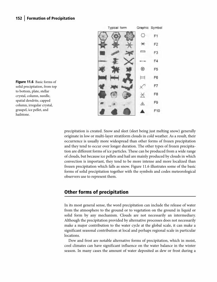
152 Formation of Precipitation
precipitation is created. Snow and sleet (sleet being just melting snow) generally
originate in low or multi-layer stratiform clouds in cold weather. As a result, their
occurrence is usually more widespread than other forms of frozen precipitation
and they tend to occur over longer duration. The other types of frozen precipita-
tion are different forms of ice particles. These can be produced from a wide range
of clouds, but because ice pellets and hail are mainly produced by clouds in which
convection is important, they tend to be more intense and more localized than
frozen precipitation which falls as snow. Figure 11.6 illustrates some of the basic
forms of solid precipitation together with the symbols and codes meteorological
observers use to represent them.
Other forms of precipitation
In its most general sense, the word precipitation can include the release of water
from the atmosphere to the ground or to vegetation on the ground in liquid or
solid form by any mechanism. Clouds are not necessarily an intermediary.
Although the precipitation provided by alternative processes does not necessarily
make a major contribution to the water cycle at the global scale, it can make a
significant seasonal contribution at local and perhaps regional scale in particular
locations.
Dew and frost are notable alternative forms of precipitation, which in moist,
cool climates can have significant influence on the water balance in the winter
season. In many cases the amount of water deposited as dew or frost during a
Figure 11.6 Basic forms of
solid precipitation, from top
to bottom, plate, stellar
crystal, column, needle,
spatial dendrite, capped
column, irregular crystal,
graupel, ice pellet, and
hailstone.
Shuttleworth_c11.indd 152Shuttleworth_c11.indd 152 11/3/2011 7:06:36 PM11/3/2011 7:06:36 PM
Formation of Precipitation 153
winter night roughly equals the amount of water evaporated during the subse-
quent daylight hours. The form of the water deposited, whether dew or frost,
depends on temperature, but the process of deposition is much the same in each
case. Nighttime loss of longwave radiation lowers the temperature of the ground
and/or vegetation and the saturated vapor pressure of the air in contact with
these; at the dew point, water or ice is deposited on the surface. The movement of
water vapor toward the surface is by turbulent diffusion. Consequently, ambient
wind speed plays a role in controlling the amount of water or ice deposited. In
light winds (0.5 to 1 m s−1), the near-surface atmosphere becomes strongly stable
and turbulent transport of vapor toward the surface and hence deposition dew or
frost is restricted. At higher wind speeds (above 3 m s−1, for example) turbulent
transport is more effective and, providing the ground is cold enough, this gives
greater deposition.
Mist and fog can also give an input of water to the surface which is sometimes
called fog drip because it may be observed as water dripping from solid surfaces
(particularly forest vegetation) that is projecting into warm, moist orographic
cloud. This phenomenon can result in a significant hydrological input, and it is not
uncommon in the mid-latitude coastal regions of western North America, Europe,
and New Zealand. Substantial precipitation also arrives as fog drip in mountain-
ous regions on eastern coasts in the tropics, indeed in some regions of Queensland
in Australia it has been reported that as much as 40% of precipitation arrives in
this way. Fog drip is particularly important from an ecological perspective in
mountainous coastal regions with little rain in Namibia and Chile, for example,
and on isolated mountains in Brazil where it provides the primary source of water
to sustain isolated ecosystems that would otherwise perish.
Important points in this chapter
● Cloud particle growth: water droplets and ice particles grow large enough
to fall from clouds as precipitation either by collision processes (called coa-
lescence between droplets, aggregation between ice particles, and accretion
between particles and droplets), or via an intermediate vapor phase when
ice particles grow at the expense of droplets in the Bergeron-Findeisen
process.
● Warm clouds: growth in warm clouds (> 0°C) is simplest to understand
because it can only occur by coalescence, but it illustrates features common
to collision growth in mixed and cold clouds, including:
— particle collisions do not always result in particle merger (see Fig. 11.1b)
— collision with merger is most efficient for larger particle collisions; and
— when large particles fall, collision growth occurs at an accelerating rate.
● Cold and mixed clouds: in cold clouds growth is only by aggregation and
particles are small and fall slowly, hence the opportunity to produce precipi-
tation is low, but in mixed clouds not only can all collision processes occur,
Shuttleworth_c11.indd 153Shuttleworth_c11.indd 153 11/3/2011 7:06:37 PM11/3/2011 7:06:37 PM

154 Formation of Precipitation
but also growth by the very efficient (often dominant) Bergeron-Findeisen
process. Hence the potential for producing precipitation size particles is
much higher.
● Which clouds produce rain?: clouds are more likely to produce rain if they
have existed for some time, have significant depth, and have high water
content.
● Precipitation form: there is distinction between (a) liquid precipitation
falling as rain or drizzle (distinguished mainly by drop size); and (b) frozen
precipitation (distinguished by morphology and whether melting or other-
wise at ground level).
● Raindrop size: ground observations suggest the number of drops falls off
exponentially with drop size at a rate related to a rainfall rate, approximately
following the Marshall-Palmer equation, i.e., −=( ) e DoN D N l
● Rain rate and kinetic energy: rain rate and the kinetic energy of rain can be
written as integrals of (empirical expressions for) terminal velocity and drop-
let size distribution: this forms the basis for soil erosion equations used in
hydrology.
● Frozen precipitation: numerous forms of frozen precipitation are recognized
but there is marked distinction between snow/sleet (from multi-layer,
stratiform clouds in cold weather) and ice pellets/hail (most intense from
convective cloud).
● Other forms of precipitation: deposition of water from the atmosphere as
dew or frost can be significant in moist, cool climates in winter, and the inter-
ception of mist or cloud by vegetation can be important locally, especially in
coastal regions.
References
Doviak, R. & Zrnic, D. (1984) Doppler Radar Weather Observations. Academic Press, New York.
Shiotsuki, Y. (1974) On the flat size distribution of drops from convective raincloud. Journal
of the Meteorological Society of Japan, 52 (1), 42–59.
Smith, J.A. (1993) Precipitation. In: Handbook of Hydrology. (ed. D. Maidment), pp. 3.1–4.1.
McGraw-Hill, New York.
Sumner, G.N. (1988) Precipitation Process and Analysis. John Wiley and Sons, Bath, UK.
Shuttleworth_c11.indd 154Shuttleworth_c11.indd 154 11/3/2011 7:06:37 PM11/3/2011 7:06:37 PM
Introduction
The measurement of precipitation appears simple, and indeed measurements of
point precipitation that are prone to systematic errors of the order of 10% have
been made for a long time, in some cases for centuries. But measurement of point
precipitation with greater accuracy than this is more difficult, and measurement of
area-average precipitation is much more difficult, particularly if the average value
required is for a large area. There are three main ways in which precipitation is
currently measured or estimated from observations. By far the most common way
is using rain gauges. Gauge measurements have been made for a long time so
gauge data has the distinct advantage that long time series are available in some
places. But gauge data also have disadvantages. They are point samples and are
consequently prone to random sampling errors. They are also prone to systematic
errors induced by selection of the gauge site and studies have identified wind-
related errors inherent to the instruments themselves.
In recent decades, ground-based radar systems have been developed that are
capable of estimating precipitation. Precipitation estimates provided by radar have
the advantage that they are real time estimates made over a large area around the
radar sensor. These attributes are extremely useful in the primary role of rainfall
radar, that is in providing information for use in short-term weather forecasting.
From the hydrological standpoint radar observations have the advantage that they
are often used to calculate area-average estimates of precipitation over pixel areas
of about 10–20 km2 rather than being point measurements. However, they have
the distinct disadvantage that they are inaccurate, even when calibrated by an
underlying gauge network and, being a recent development, there are as yet no
long-term records of radar-estimated precipitation.
Indirect estimates of precipitation are also made from remote sensing data using
several different approaches. Again there are problems with measurement accuracy
12 Precipitation Measurement and Observation
Terrestrial Hydrometeorology, First Edition. W. James Shuttleworth.
© 2012 John Wiley & Sons, Ltd. Published 2012 by John Wiley & Sons, Ltd.
Shuttleworth_c12.indd 155Shuttleworth_c12.indd 155 11/3/2011 7:03:41 PM11/3/2011 7:03:41 PM
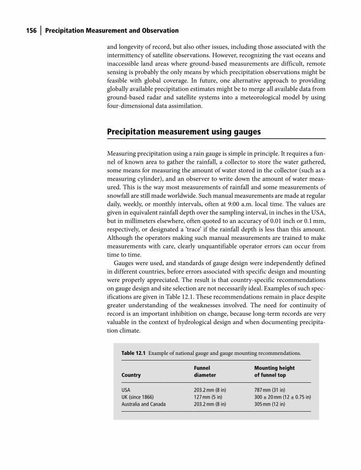
156 Precipitation Measurement and Observation
and longevity of record, but also other issues, including those associated with the
intermittency of satellite observations. However, recognizing the vast oceans and
inaccessible land areas where ground-based measurements are difficult, remote
sensing is probably the only means by which precipitation observations might be
feasible with global coverage. In future, one alternative approach to providing
globally available precipitation estimates might be to merge all available data from
ground-based radar and satellite systems into a meteorological model by using
four-dimensional data assimilation.
Precipitation measurement using gauges
Measuring precipitation using a rain gauge is simple in principle. It requires a fun-
nel of known area to gather the rainfall, a collector to store the water gathered,
some means for measuring the amount of water stored in the collector (such as a
measuring cylinder), and an observer to write down the amount of water meas-
ured. This is the way most measurements of rainfall and some measurements of
snowfall are still made worldwide. Such manual measurements are made at regular
daily, weekly, or monthly intervals, often at 9:00 a.m. local time. The values are
given in equivalent rainfall depth over the sampling interval, in inches in the USA,
but in millimeters elsewhere, often quoted to an accuracy of 0.01 inch or 0.1 mm,
respectively, or designated a ‘trace’ if the rainfall depth is less than this amount.
Although the operators making such manual measurements are trained to make
measurements with care, clearly unquantifiable operator errors can occur from
time to time.
Gauges were used, and standards of gauge design were independently defined
in different countries, before errors associated with specific design and mounting
were properly appreciated. The result is that country-specific recommendations
on gauge design and site selection are not necessarily ideal. Examples of such spec-
ifications are given in Table 12.1. These recommendations remain in place despite
greater understanding of the weaknesses involved. The need for continuity of
record is an important inhibition on change, because long-term records are very
valuable in the context of hydrological design and when documenting precipita-
tion climate.
Table 12.1 Example of national gauge and gauge mounting recommendations.
Country Funnel diameter
Mounting height of funnel top
USA 203.2 mm (8 in) 787 mm (31 in)UK (since 1866) 127 mm (5 in) 300 ± 20 mm (12 ± 0.75 in)Australia and Canada 203.2 mm (8 in) 305 mm (12 in)
Shuttleworth_c12.indd 156Shuttleworth_c12.indd 156 11/3/2011 7:03:42 PM11/3/2011 7:03:42 PM
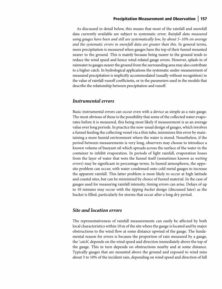
Precipitation Measurement and Observation 157
As discussed in detail below, this means that most of the rainfall and snowfall
data currently available are subject to systematic error. Rainfall data measured
using gauges have been and still are systematically low, by about 5–10% on average
and the systematic errors in snowfall data are greater than this. In general terms,
more precipitation is measured when gauges have the top of their funnel mounted
nearer to the ground. This is mainly because being nearer to the ground tends to
reduce the wind speed and hence wind-related gauge errors. However, splash-in of
rainwater to gauges nearer the ground from the surrounding area may also contribute
to a higher catch. In hydrological applications the systematic under-measurement of
measured precipitation is implicitly accommodated (usually without recognition) in
the value of rainfall-runoff coefficients, or in the parameters used in the models that
describe the relationship between precipitation and runoff.
Instrumental errors
Basic instrumental errors can occur even with a device as simple as a rain gauge.
The most obvious of these is the possibility that some of the collected water evapo-
rates before it is measured, this being most likely if measurement is as an average
value over long periods. In practice the now-usual design of gauges, which involves
a funnel feeding the collecting vessel via a thin tube, minimizes this error by main-
taining a more humid environment where the water is stored. Nonetheless, if the
period between measurements is very long, observers may choose to introduce a
known volume of buoyant oil which spreads across the surface of the water in the
container to inhibit evaporation. In periods of light rainfall, evaporation losses
from the layer of water that wets the funnel itself (sometimes known as wetting
errors) may be significant in percentage terms. In humid atmospheres, the oppo-
site problem can occur, with water condensed onto cold metal gauges to increase
the apparent rainfall. This latter problem is most likely to occur at high latitude
and coastal sites, but can be minimized by choice of funnel material. In the case of
gauges used for measuring rainfall intensity, timing errors can arise. Delays of up
to 10 minutes may occur with the tipping bucket design (discussed later) as the
bucket is filled, particularly for storms that occur after a long dry period.
Site and location errors
The representativeness of rainfall measurements can easily be affected by both
local characteristics within 10 m of the site where the gauge is located and by major
obstructions to the wind flow at some distance upwind of the gauge. The funda-
mental reason for errors is because the proportion of rain measured by a gauge,
the ‘catch’, depends on the wind speed and direction immediately above the top of
the gauge. This in turn depends on obstructions nearby and at some distance.
Typically gauges that are mounted above the ground and exposed to wind miss
about 5 to 10% of the incident rain, depending on wind speed and direction of fall
Shuttleworth_c12.indd 157Shuttleworth_c12.indd 157 11/3/2011 7:03:42 PM11/3/2011 7:03:42 PM
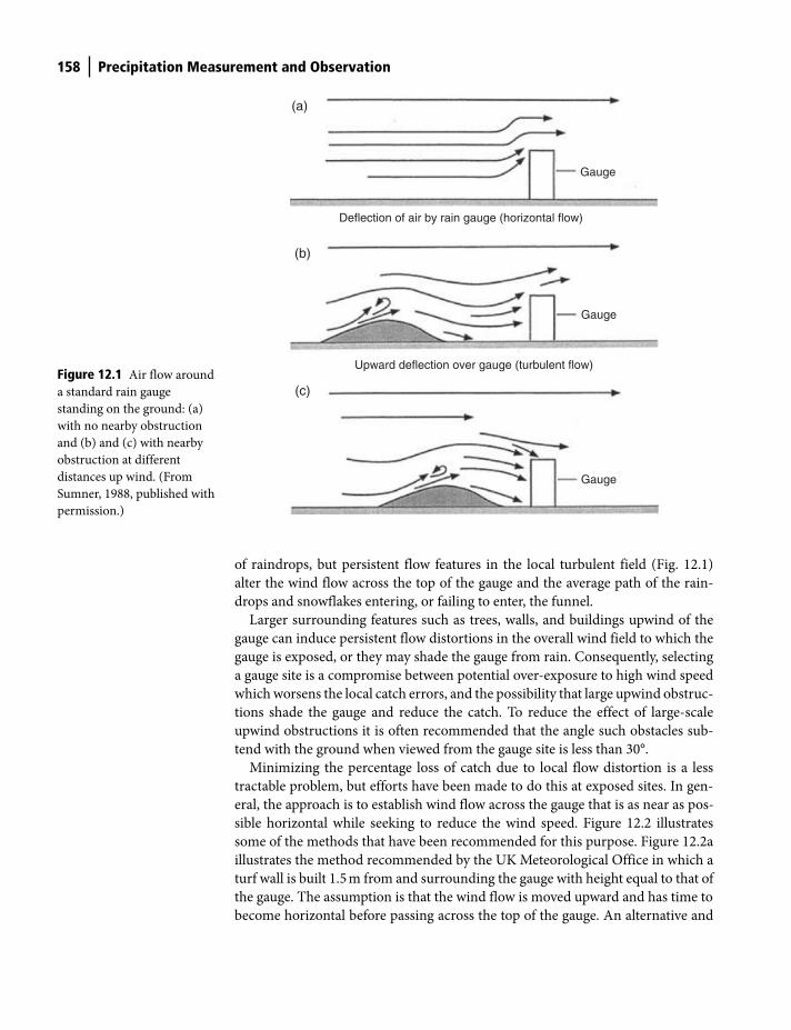
158 Precipitation Measurement and Observation
of raindrops, but persistent flow features in the local turbulent field (Fig. 12.1)
alter the wind flow across the top of the gauge and the average path of the rain-
drops and snowflakes entering, or failing to enter, the funnel.
Larger surrounding features such as trees, walls, and buildings upwind of the
gauge can induce persistent flow distortions in the overall wind field to which the
gauge is exposed, or they may shade the gauge from rain. Consequently, selecting
a gauge site is a compromise between potential over-exposure to high wind speed
which worsens the local catch errors, and the possibility that large upwind obstruc-
tions shade the gauge and reduce the catch. To reduce the effect of large-scale
upwind obstructions it is often recommended that the angle such obstacles sub-
tend with the ground when viewed from the gauge site is less than 30°.
Minimizing the percentage loss of catch due to local flow distortion is a less
tractable problem, but efforts have been made to do this at exposed sites. In gen-
eral, the approach is to establish wind flow across the gauge that is as near as pos-
sible horizontal while seeking to reduce the wind speed. Figure 12.2 illustrates
some of the methods that have been recommended for this purpose. Figure 12.2a
illustrates the method recommended by the UK Meteorological Office in which a
turf wall is built 1.5 m from and surrounding the gauge with height equal to that of
the gauge. The assumption is that the wind flow is moved upward and has time to
become horizontal before passing across the top of the gauge. An alternative and
Gauge
Gauge
Deflection of air by rain gauge (horizontal flow)
(a)
Upward deflection over gauge (turbulent flow)
Gauge
(b)
(c)Figure 12.1 Air flow around
a standard rain gauge
standing on the ground: (a)
with no nearby obstruction
and (b) and (c) with nearby
obstruction at different
distances up wind. (From
Sumner, 1988, published with
permission.)
Shuttleworth_c12.indd 158Shuttleworth_c12.indd 158 11/3/2011 7:03:42 PM11/3/2011 7:03:42 PM
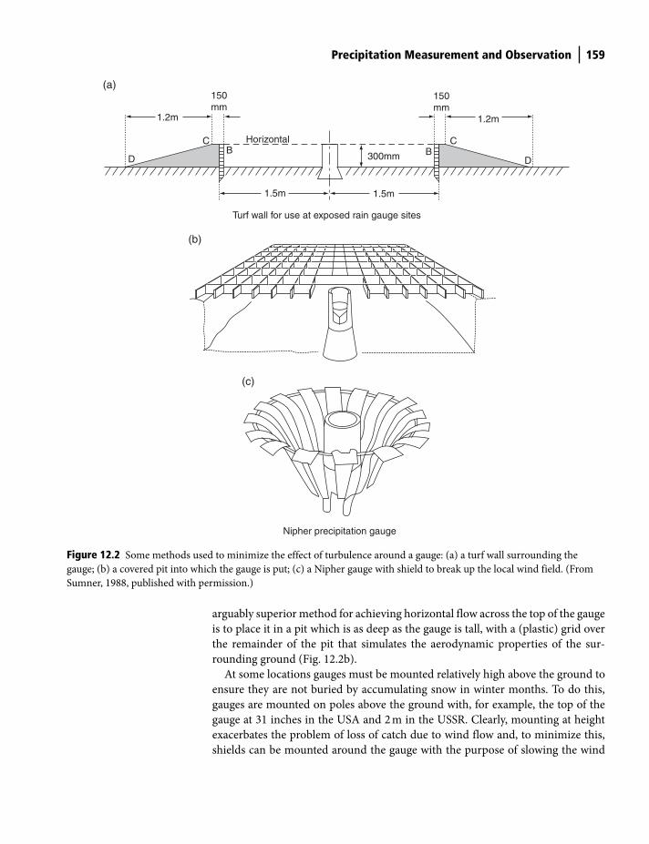
Precipitation Measurement and Observation 159
arguably superior method for achieving horizontal flow across the top of the gauge
is to place it in a pit which is as deep as the gauge is tall, with a (plastic) grid over
the remainder of the pit that simulates the aerodynamic properties of the sur-
rounding ground (Fig. 12.2b).
At some locations gauges must be mounted relatively high above the ground to
ensure they are not buried by accumulating snow in winter months. To do this,
gauges are mounted on poles above the ground with, for example, the top of the
gauge at 31 inches in the USA and 2 m in the USSR. Clearly, mounting at height
exacerbates the problem of loss of catch due to wind flow and, to minimize this,
shields can be mounted around the gauge with the purpose of slowing the wind
D
1.2m
150mm
HorizontalCB
1.5m
300mm
1.5m
BC
150mm
1.2m
D
Turf wall for use at exposed rain gauge sites
(a)
(b)
(c)
Nipher precipitation gauge
Figure 12.2 Some methods used to minimize the effect of turbulence around a gauge: (a) a turf wall surrounding the
gauge; (b) a covered pit into which the gauge is put; (c) a Nipher gauge with shield to break up the local wind field. (From
Sumner, 1988, published with permission.)
Shuttleworth_c12.indd 159Shuttleworth_c12.indd 159 11/3/2011 7:03:43 PM11/3/2011 7:03:43 PM
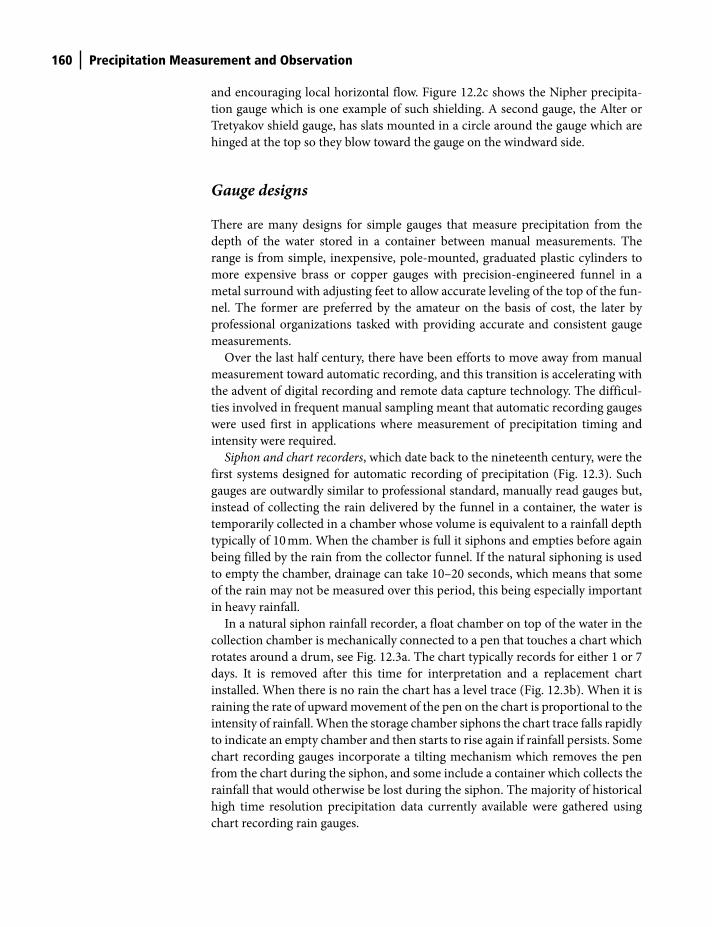
160 Precipitation Measurement and Observation
and encouraging local horizontal flow. Figure 12.2c shows the Nipher precipita-
tion gauge which is one example of such shielding. A second gauge, the Alter or
Tretyakov shield gauge, has slats mounted in a circle around the gauge which are
hinged at the top so they blow toward the gauge on the windward side.
Gauge designs
There are many designs for simple gauges that measure precipitation from the
depth of the water stored in a container between manual measurements. The
range is from simple, inexpensive, pole-mounted, graduated plastic cylinders to
more expensive brass or copper gauges with precision-engineered funnel in a
metal surround with adjusting feet to allow accurate leveling of the top of the fun-
nel. The former are preferred by the amateur on the basis of cost, the later by
professional organizations tasked with providing accurate and consistent gauge
measurements.
Over the last half century, there have been efforts to move away from manual
measurement toward automatic recording, and this transition is accelerating with
the advent of digital recording and remote data capture technology. The difficul-
ties involved in frequent manual sampling meant that automatic recording gauges
were used first in applications where measurement of precipitation timing and
intensity were required.
Siphon and chart recorders, which date back to the nineteenth century, were the
first systems designed for automatic recording of precipitation (Fig. 12.3). Such
gauges are outwardly similar to professional standard, manually read gauges but,
instead of collecting the rain delivered by the funnel in a container, the water is
temporarily collected in a chamber whose volume is equivalent to a rainfall depth
typically of 10 mm. When the chamber is full it siphons and empties before again
being filled by the rain from the collector funnel. If the natural siphoning is used
to empty the chamber, drainage can take 10–20 seconds, which means that some
of the rain may not be measured over this period, this being especially important
in heavy rainfall.
In a natural siphon rainfall recorder, a float chamber on top of the water in the
collection chamber is mechanically connected to a pen that touches a chart which
rotates around a drum, see Fig. 12.3a. The chart typically records for either 1 or 7
days. It is removed after this time for interpretation and a replacement chart
installed. When there is no rain the chart has a level trace (Fig. 12.3b). When it is
raining the rate of upward movement of the pen on the chart is proportional to the
intensity of rainfall. When the storage chamber siphons the chart trace falls rapidly
to indicate an empty chamber and then starts to rise again if rainfall persists. Some
chart recording gauges incorporate a tilting mechanism which removes the pen
from the chart during the siphon, and some include a container which collects the
rainfall that would otherwise be lost during the siphon. The majority of historical
high time resolution precipitation data currently available were gathered using
chart recording rain gauges.
Shuttleworth_c12.indd 160Shuttleworth_c12.indd 160 11/3/2011 7:03:43 PM11/3/2011 7:03:43 PM
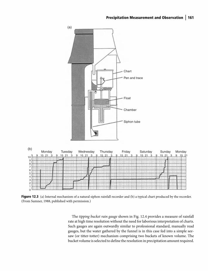
Precipitation Measurement and Observation 161
The tipping bucket rain gauge shown in Fig. 12.4 provides a measure of rainfall
rate at high time resolution without the need for laborious interpretation of charts.
Such gauges are again outwardly similar to professional standard, manually read
gauges, but the water gathered by the funnel is in this case fed into a simple see-
saw (or titter-totter) mechanism comprising two buckets of known volume. The
bucket volume is selected to define the resolution in precipitation amount required.
Chart
(a)
(b)
Pen and trace
Float
Chamber
Siphon tube
103 9 15 21
Monday Tuesday Wednesday Thursday Friday Saturday Sunday Monday3 9 15 21 3 9 15 21 3 9 15 21 3 9 15 21 3 9 15 21 3 9 15 21 3 9 15 21
9876543210
Figure 12.3 (a) Internal mechanism of a natural siphon rainfall recorder and (b) a typical chart produced by the recorder.
(From Sumner, 1988, published with permission.)
Shuttleworth_c12.indd 161Shuttleworth_c12.indd 161 11/3/2011 7:03:43 PM11/3/2011 7:03:43 PM
162 Precipitation Measurement and Observation
The water fills one bucket and, when this is full, the bucket assembly tips, emptying
the first bucket and simultaneously positioning the second bucket under the funnel
outlet. The second bucket then fills and when it is full the system tips in the
opposite direction. Each time a tip occurs, an electrical signal is sent to a digital
recorder that either records the time of the tip if high frequency intensity
measurements are required, or the number of tips over a predefined interval if
integrated rainfall amount is required. The precision of the measurement is limited
by the volume of the bucket. Smaller buckets give higher precision, but they can
pose problems in intense rainfall when water loss may occur because the tip rate is
high. The simplicity of the mechanism involved in the tipping bucket rain gauge
means it is a robust, reliable and much used instrument. However, in recent years
the advent of devices (strain gauges/load cells) with electronic output that are
capable of accurately measuring the weight of water stored in the chamber below
a gauge funnel has resulted in an alternative to the tipping bucket rain gauge that
has few moving parts and potentially requires less servicing because of this.
Areal representativeness of gauge measurements
Gauges provide point samples of the precipitation at a particular place. Comparison
with other data sampling challenges puts the rainfall sampling issue into
Splash guard
Splash guard
Cable torecorder
Mercoid switch
(a)Tipping bucket
(b)
Figure 12.4 A tipping bucket rain gauge: (a) simplified diagram of internal mechanism; (b) external view of the gauge
assembly. (From Sumner, 1988, published with permission.)
Shuttleworth_c12.indd 162Shuttleworth_c12.indd 162 11/3/2011 7:03:44 PM11/3/2011 7:03:44 PM
Precipitation Measurement and Observation 163
perspective. The polls used to gauge public opinion, for example, typically sample
a few thousand out of several tens of millions of people, and so are a sample of
order 0.1%. In comparison, the rain gauge network used in the United Kingdom
has about two gauges with funnel area 0.0127 m2 to sample an area of 100 km2
(a 5 × 10⁻¹² % sample), and the network used in the United States of America has a
sampling density approximately one tenth of this.
The global challenge of providing estimates of area-average precipitation is
further exacerbated by the fact that gauge densities are very substantially less
than those just mentioned for the UK and USA. The location of available gauges
is also heavily biased, with most gauges located in wealthier, developed coun-
tries. Even in countries where there are many gauges, the gauge sample is heavily
biased toward centers of population and, because of this, to lowland sites. This is
an issue because much of the surface water used to provide water resources for
human use falls as precipitation in sparsely populated regions with significant
topography.
When seeking to evaluate the representativeness of available gauge data, typical
questions asked are, ‘How representative are a set of gauges in giving average rain-
fall when there is systematic spatial variability which may be related to topography
and/or mean rainfall gradients?’, or, ‘What is the minimum gauge density needed
to sample spatial rainfall pattern and total water volume of a rain event?’ In gen-
eral, there is a need for a denser network when seeking to determine short-term
rainfall totals. For example, in a temperate climate a study in which a 9-gauge
network was used to measure rainfall across a small, 20 m grid gave gauge-to-
gauge variations of ±5% in the measured monthly total, but ±8% in single storm
totals. Studies in the semi-arid climate of southern Arizona, where much of the
rain falls in thunderstorms, suggest that one gauge every 2.4 km is needed to pro-
vide an adequate estimate of the annual water balance for a catchment of area
25 km2 (Sumner 1988).
When installing a gauge network to document precipitation pattern and
area-average precipitation, the optimum sampling pattern should recognize
known systematic variations. In flat regions and in urban environments, it is
generally considered best to install gauges on a rectangular grid, with a gauge
at each intersection of the grid. In regions with steep topography, which is often
the case for experimental catchments in which hydrological studies are made,
the recommended procedure is to define ‘hill slope elements’ on the basis
of these having similar slope and aspect, and to locate a rain gauge in the mid-
dle of each. If there is evidence of a rainfall gradient, or such a gradient might
realistically be expected (because the ground is sloping, or sampling is away
from a coast where weather systems move onshore), the preferred sampling
will be along the gradient.
One strategy that can be used is first to make an educated guess at the most
appropriate sampling strategy for the situation under study, then collect data for a
trial period and analyze the data, and then optimize the gauge arrangement, if
necessary. The correlation coefficient between all the gauges in the network for the
duration over which rainfall estimates are required may be used as a numerical
Shuttleworth_c12.indd 163Shuttleworth_c12.indd 163 11/3/2011 7:03:44 PM11/3/2011 7:03:44 PM
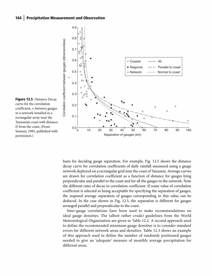
164 Precipitation Measurement and Observation
basis for deciding gauge separation. For example, Fig. 12.5 shows the distance
decay curve for correlation coefficients of daily rainfall measured using a gauge
network deployed on a rectangular grid near the coast of Tanzania. Average curves
are drawn for correlation coefficient as a function of distance for gauges lying
perpendicular and parallel to the coast and for all the gauges in the network. Note
the different rates of decay in correlation coefficient. If some value of correlation
coefficient is selected as being acceptable for specifying the separation of gauges,
the required average separation of gauges corresponding to this value can be
deduced. In the case shown in Fig. 12.5, the separation is different for gauges
arranged parallel and perpendicular to the coast.
Inter-gauge correlations have been used to make recommendations on
ideal gauge densities. The (albeit rather crude) guidelines from the World
Meteorological Organization are given in Table 12.2. A second approach used
to define the recommended minimum gauge densities is to consider standard
errors for different network areas and densities. Table 12.3 shows an example
of this approach used to define the number of randomly positioned gauges
needed to give an ‘adequate’ measure of monthly average precipitation for
different areas.
0.9
0.8
0.7
0.6
0.5r
Cor
rela
tion
coef
ficie
nt b
etw
een
gaug
es (
dim
ensi
onle
ss)
0.4
0.3
0.2
0.1
0.00 10 20 30 40
Separation of gauges (km)
50 60 70 80 90 100
Coastal All
Parallel to coast
Normal to coast
Regional
Network
Figure 12.5 Distance Decay
curve for the correlation
coefficient, r, between gauges
in a network installed in a
rectangular array near the
Tanzanian coast with distance
D from the coast. (From
Sumner, 1983, published with
permission.)
Shuttleworth_c12.indd 164Shuttleworth_c12.indd 164 11/3/2011 7:03:44 PM11/3/2011 7:03:44 PM
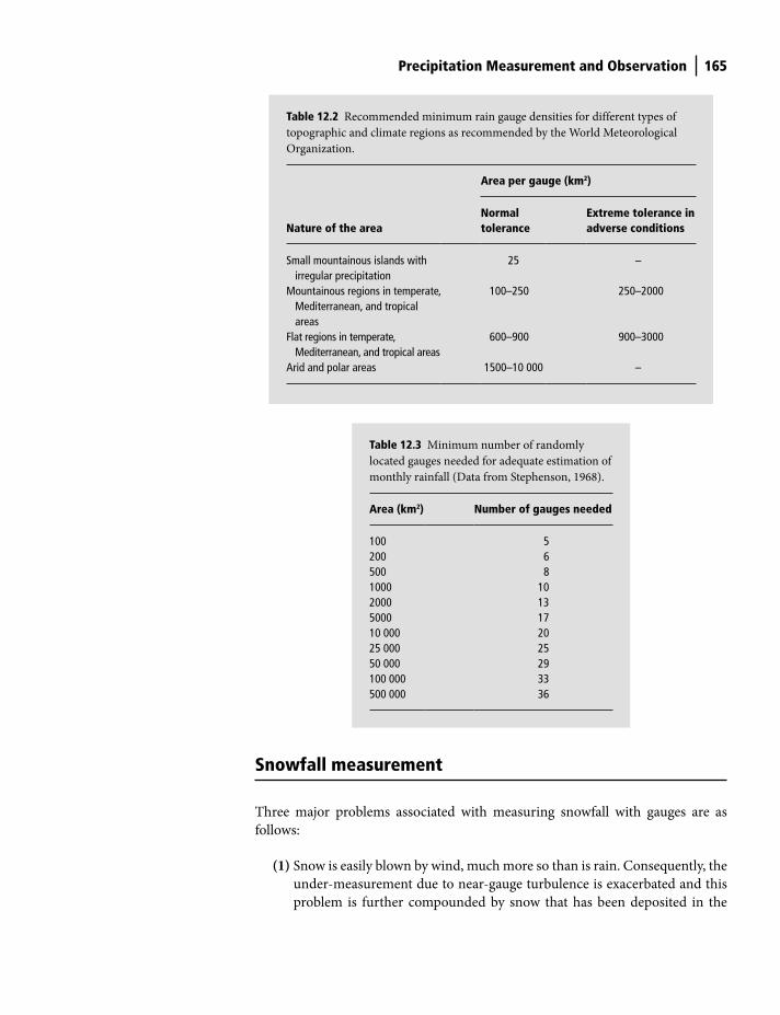
Precipitation Measurement and Observation 165
Snowfall measurement
Three major problems associated with measuring snowfall with gauges are as
follows:
(1) Snow is easily blown by wind, much more so than is rain. Consequently, the
under-measurement due to near-gauge turbulence is exacerbated and this
problem is further compounded by snow that has been deposited in the
Table 12.2 Recommended minimum rain gauge densities for different types of
topographic and climate regions as recommended by the World Meteorological
Organization.
Nature of the area
Area per gauge (km2)
Normal tolerance
Extreme tolerance in adverse conditions
Small mountainous islands with irregular precipitation
25 –
Mountainous regions in temperate, Mediterranean, and tropical areas
100–250 250–2000
Flat regions in temperate, Mediterranean, and tropical areas
600–900 900–3000
Arid and polar areas 1500–10 000 –
Table 12.3 Minimum number of randomly
located gauges needed for adequate estimation of
monthly rainfall (Data from Stephenson, 1968).
Area (km2) Number of gauges needed
100 5200 6500 81000 102000 135000 1710 000 2025 000 2550 000 29100 000 33500 000 36
Shuttleworth_c12.indd 165Shuttleworth_c12.indd 165 11/3/2011 7:03:45 PM11/3/2011 7:03:45 PM
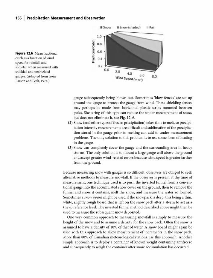
166 Precipitation Measurement and Observation
gauge subsequently being blown out. Sometimes ‘blow fences’ are set up
around the gauge to protect the gauge from wind. These shielding fences
may perhaps be made from horizontal plastic strips mounted between
poles. Sheltering of this type can reduce the under-measurement of snow,
but does not eliminate it, see Fig. 12. 6.
(2) Snow (and other types of frozen precipitation) takes time to melt, so precipi-
tation intensity measurements are difficult and sublimation of the precipita-
tion stored in the gauge prior to melting can add to under-measurement
problems. The only solution to this problem is to use some form of heating
in the gauge.
(3) Snow can completely cover the gauge and the surrounding area in heavy
storms. The only solution is to mount a large gauge well above the ground
and accept greater wind-related errors because wind speed is greater farther
from the ground.
Because measuring snow with gauges is so difficult, observers are obliged to seek
alternative methods to measure snowfall. If the observer is present at the time of
measurement, one technique used is to push the inverted funnel from a conven-
tional gauge into the accumulated snow cover on the ground, then to remove the
funnel and snow it contains, melt the snow, and measure the water so formed.
Sometimes a snow board might be used if the snowpack is deep, this being a thin,
white, slightly rough board that is left on the snow pack after a storm to act as a
(new) reference level. The inverted funnel method described above might then be
used to measure the subsequent snow deposited.
One very common approach to measuring snowfall is simply to measure the
height of the snow and to assume a density for the snow pack. Often the snow is
assumed to have a density of 10% of that of water. A snow board might again be
used with this approach to allow measurement of increments in the snow pack.
More than 80% of Canadian meteorological stations use this approach. Another
simple approach is to deploy a container of known weight containing antifreeze
and subsequently to weigh the container after snow accumulation has occurred.
Figure 12.6 Mean fractional
catch as a function of wind
speed for rainfall, and
snowfall when measured with
shielded and unshielded
gauges. (Adapted from from
Larson and Peck, 1974.)
Shuttleworth_c12.indd 166Shuttleworth_c12.indd 166 11/3/2011 7:03:45 PM11/3/2011 7:03:45 PM
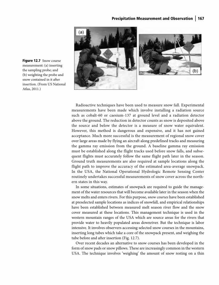
Precipitation Measurement and Observation 167
Radioactive techniques have been used to measure snow fall. Experimental
measurements have been made which involve installing a radiation source
such as cobalt-60 or caesium-137 at ground level and a radiation detector
above the ground. The reduction in detector counts as snow is deposited above
the source and below the detector is a measure of snow water equivalent.
However, this method is dangerous and expensive, and it has not gained
acceptance. Much more successful is the measurement of regional snow cover
over large areas made by flying an aircraft along predefined tracks and measuring
the gamma ray emission from the ground. A baseline gamma ray emission
must be established along the flight tracks used before snow falls, and subse-
quent flights must accurately follow the same flight path later in the season.
Ground truth measurements are also required at sample locations along the
flight path to improve the accuracy of the estimated area-average snowpack.
In the USA, the National Operational Hydrologic Remote Sensing Center
routinely undertakes successful measurements of snow cover across the north-
ern states in this way.
In some situations, estimates of snowpack are required to guide the manage-
ment of the water resources that will become available later in the season when the
snow melts and enters rivers. For this purpose, snow courses have been established
at preselected sample locations as indices of snowfall, and empirical relationships
have been established between measured melt season river flow and the snow
cover measured at these locations. This management technique is used in the
western mountain ranges of the USA which are source areas for the rivers that
provide water to heavily populated areas downriver. But the technique is labor
intensive. It involves observers accessing selected snow courses in the mountains,
inserting long tubes which take a core of the snowpack present, and weighing the
tube before and after insertion (Fig. 12.7).
Over recent decades an alternative to snow courses has been developed in the
form of snow pads or snow pillows. These are increasingly common in the western
USA. The technique involves ‘weighing’ the amount of snow resting on a thin
Figure 12.7 Snow course
measurement: (a) inserting
the sampling probe; and
(b) weighting the probe and
snow contained in it after
insertion. (From US National
Atlas, 2011.)
Shuttleworth_c12.indd 167Shuttleworth_c12.indd 167 11/3/2011 7:03:45 PM11/3/2011 7:03:45 PM
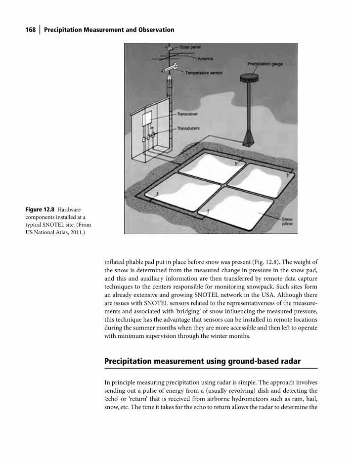
168 Precipitation Measurement and Observation
inflated pliable pad put in place before snow was present (Fig. 12.8). The weight of
the snow is determined from the measured change in pressure in the snow pad,
and this and auxiliary information are then transferred by remote data capture
techniques to the centers responsible for monitoring snowpack. Such sites form
an already extensive and growing SNOTEL network in the USA. Although there
are issues with SNOTEL sensors related to the representativeness of the measure-
ments and associated with ‘bridging’ of snow influencing the measured pressure,
this technique has the advantage that sensors can be installed in remote locations
during the summer months when they are more accessible and then left to operate
with minimum supervision through the winter months.
Precipitation measurement using ground-based radar
In principle measuring precipitation using radar is simple. The approach involves
sending out a pulse of energy from a (usually revolving) dish and detecting the
‘echo’ or ‘return’ that is received from airborne hydrometeors such as rain, hail,
snow, etc. The time it takes for the echo to return allows the radar to determine the
Figure 12.8 Hardware
components installed at a
typical SNOTEL site. (From
US National Atlas, 2011.)
Shuttleworth_c12.indd 168Shuttleworth_c12.indd 168 11/3/2011 7:03:45 PM11/3/2011 7:03:45 PM
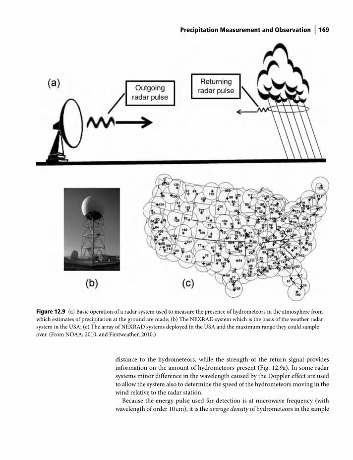
Precipitation Measurement and Observation 169
distance to the hydrometeors, while the strength of the return signal provides
information on the amount of hydrometeors present (Fig. 12.9a). In some radar
systems minor difference in the wavelength caused by the Doppler effect are used
to allow the system also to determine the speed of the hydrometeors moving in the
wind relative to the radar station.
Because the energy pulse used for detection is at microwave frequency (with
wavelength of order 10 cm), it is the average density of hydrometeors in the sample
Figure 12.9 (a) Basic operation of a radar system used to measure the presence of hydrometeors in the atmosphere from
which estimates of precipitation at the ground are made; (b) The NEXRAD system which is the basis of the weather radar
system in the USA; (c) The array of NEXRAD systems deployed in the USA and the maximum range they could sample
over. (From NOAA, 2010, and Firstweather, 2010.)
Shuttleworth_c12.indd 169Shuttleworth_c12.indd 169 11/3/2011 7:03:46 PM11/3/2011 7:03:46 PM
170 Precipitation Measurement and Observation
volume that is detected. The average returned power, P, received at the radar
receiver from a hydrometeor-filled atmosphere at range, r, between the radar and
the measured sample is given by:
=2
r rC A ZPr
(12.1)
where Cr is a constant determined by the design of the system and dependent on
the beam width, antenna gain, wavelength, and pulse duration, etc; Ar is a factor
representing the signal attenuation during its transit through the atmosphere; and
Z is the radar reflectivity factor for the volume of atmosphere sampled by the radar
beam which is usually expressed in units of mm6 m−3.
The estimated rainfall rate in mm hr−1, R, is related to the radar reflectivity fac-
tor, Z, by a semi-empirical power law often called the Z-R relationship with the
form:
bR aZ= (12.2)
At microwave wavelengths, the return signal is generated by Rayleigh scattering,
which means the strength of the return signal expressed in the form of the radar
reflectivity factor is proportional to the sixth power of the diameter of the hydro-
meteors. Consequently, the sensitivity of the system is strongly influenced by the
unknown range of hydrometeor diameters present in the sample. The values of the
empirical parameters a and b in Equation (12.2) are determined by the very vari-
able size spectrum of the hydrometeors and are poorly defined. For the WSR-88D
network that covers the USA (see, for example, http://www.erh.noaa.gov/ohrfc/
ZRlisting.shtml) typical values for a are in the range 130–300 and for b in the
range 1.4–2.0, which implies the system calibration might vary by substantial fac-
tors between rainstorms. A further source of error in the system is that the hydro-
meteors are detected well above the surface so there is potential for them to
evaporate to a variable extent as they fall to the ground. Because the calibration of
the system is inherently poor, when used to estimate rainfall for hydrological
applications radar observations must be continuously recalibrated by merging the
radar estimates with observations from an underlying network of gauges. The
resulting data fields so created are called merged products.
The primary application of radar data is to support weather forecasting and
NEXRAD systems of the type shown in Fig. 12.9b have been deployed for this
purpose across the USA in the network shown in Fig. 12.9c. Notwithstanding the
serious calibration issues associated with radar-based precipitation observations,
they have important properties that are potentially of great value for hydrological
science. The data provided as merged radar-gauge products are area-average esti-
mates of precipitation typically for 4 km by 4 km pixels that are available with high
temporal resolution for intervals of the order of minutes. Such data could greatly
enhance skill in flood forecasting and once they have been available for long
enough, also water resource estimation. However, the very different nature of
Shuttleworth_c12.indd 170Shuttleworth_c12.indd 170 11/3/2011 7:03:46 PM11/3/2011 7:03:46 PM

Precipitation Measurement and Observation 171
these data mean rainfall-runoff relationships and the parameters used in hydro-
logical models will need recalibration.
Precipitation measurement using satellite systems
At the present time the quest to provide estimates of precipitation from satellite
observations is an extremely active area of hydrometeorological research. The
motivation for this research is that estimates derived in this way are likely the only
means by which measurement-based (as opposed to model-based) estimates of
precipitation can be made for the entire globe, including the two-thirds of the
globe covered with ocean and for the vast areas of land that are hard to access.
Exploratory methods have reached the stage where they can provide estimates
that are at least of qualitative value and increasingly also of quantitative value
when averaged over large areas and long periods and they are used to guide the
development of GCMs. Because the rate of development in this field of hydrome-
teorology is currently so rapid, it is likely that detailed documentation of current
methods will be quickly outdated. Consequently, the discussion below is given in
general terms. Broadly speaking, three main methods are used, which are based
around:
(1) cloud mapping and characterization;
(2) passive measurement of cloud properties; and
(3) spaceborne radar.
Modern methods for deriving precipitation from remotely sensed information
often use a combination of more than one of these three basic approaches.
Cloud mapping and characterization
This was the method used in the earliest efforts to derive estimates of precipitation
from satellite data. The basis of the approach is to calibrate and exploit empirical
relationships between the precipitation at a location, and the extent and nature of
the overlying cloud as identified from space. Cloud indices are derived based on
remotely sensed characteristics which are then empirically related to rainfall
intensity. In general terms, the estimated rainfall falling over a defined period, Rsat,
is calculated from an equation with the form:
[ ], ( )satR f c i a= ¢
(12.3)
where f´ denotes an empirical function, c is the area of cloud measured by the
satellite, i denotes a cloud type, and a its altitude. This index of cloud development
can be related to available rain gauge data over the same period and, once
Shuttleworth_c12.indd 171Shuttleworth_c12.indd 171 11/3/2011 7:03:48 PM11/3/2011 7:03:48 PM

172 Precipitation Measurement and Observation
calibration has been made, future satellite imagery used to make estimates of
probable precipitation.
Estimates of rainfall rate are still made using knowledge of the extent and
nature of cloud but it has become usual to merge such knowledge with additional
meteorological information derived from satellite observations. The TOVS
precipitation estimate and the AIRS precipitation product are examples. Data from
the Television Infrared Operational Satellite (TIROS) Operational Vertical Sounder
(TOVS) instruments on board polar-orbiting platforms and AIRS instrument
aboard the Earth Observing System Aqua polar-orbiting satellite are both processed
to provide meteorological statistics. These two precipitation products then infer
precipitation from deep extensive clouds using a multiple regression relationship
between collocated rain gauge measurements and the several satellite data streams
(related to cloud volume, cloud-top pressure, fractional cloud cover, and relative
humidity profile). The relationship used is allowed to vary with season and latitude
and separate relationships are used for ocean and land.
Passive measurement of cloud properties
The essential basis of this approach is to calibrate and exploit empirical relation-
ships between precipitation at a particular location and physical characteristics of
the overlying cloud measured by remote sensing systems. The most commonly
used physical characteristic is the brightness temperature of the top of cloud as
diagnosed by the measured outward longwave radiation (OLR). Colder cloud top
temperature implies deeper clouds with more convective ascent and a greater like-
lihood of rain. Estimates based on cloud top temperature have greatest probability
of success in regions and at times where convective rainfall is dominant, i.e., in the
tropics, and in the summer season elsewhere.
One significant satellite precipitation estimate based on this approach is the
Global Precipitation Index (GPI), which uses three-hourly infrared images provided
by three geostationary satellites. An empirical relationship based on data from the
Global Atmospheric Research Programme (GARP) Atlantic Tropical Experiment
(GATE) is used for this product. For a brightness temperature ≤ 235 K, a rain rate of
3 mm hr−1 is assigned, while for a brightness temperature >235 K, a rain rate of
0 mm/hour is assigned. The GPI estimate works best over space and time averages
of at least 250 km and 6 hours, respectively, and in oceanic regions with deep
convection. Several other precipitation products based on OLR are also available.
Some, such as the PERSIANN precipitation product, have developed
interrelationships using neural networks rather than using fixed formulae or linear
regression.
At microwave frequencies, the atmosphere is almost transparent where no
precipitating clouds occur. Where there is high humidity and particularly where
there are precipitating clouds, microwave emissivity and absorption is greater.
Consequently, data from satellite sensors operating in the microwave waveband
can contribute information relevant to remote sensing-based precipitation
Shuttleworth_c12.indd 172Shuttleworth_c12.indd 172 11/3/2011 7:03:49 PM11/3/2011 7:03:49 PM
Precipitation Measurement and Observation 173
products. One microwave-based data product is the Goddard Profiling Algorithm
(GPROF) fractional occurrence of precipitation which gives the fraction of area
with precipitation on a 0.5° by 0.5° grid over ocean. The algorithm applies a
Bayesian inversion method to the observed microwave brightness temperatures
using an extensive library of cloud-model-based relations between hydrometeor
profiles and microwave brightness temperatures. Each hydrometeor profile is
associated with a surface precipitation rate.
There is value in seeking to use the many alternative sources of remotely sensed
data relevant to estimating precipitation now available to provide a single best esti-
mate. The Global Precipitation Climatology Project (GPCP) seeks to derive such a
preferred satellite precipitation data set by selecting and merging data from many
sources.
Spaceborne radar
Good progress has been made toward remote sensing precipitation using
space-based radar broadly similar to that used in ground-based systems, and
there are plans to develop this approach further. The precipitation radar used
in the Tropical Rainfall Measuring mission (TRMM) was the first spaceborne
instrument designed to provide three-dimensional maps of storm structure.
These measurements yield information on the intensity and distribution of the
rain, on rain type and storm depth, and on the height at which the snow melts
into rain. TRMM had a horizontal resolution at the ground of about five kilom-
eters and a swath width of 247 kilometers. One important feature was its ability
to provide vertical profiles of the rain and snow from the surface to a height of
~20 kilometers. The TRMM radar was able to detect fairly light rain rates down
to about 0.7 mm hr−1, but it was less successful when detecting intense rain
rates.
Providing enough power to detect the weak return echo from the raindrops
when seen from orbital height is a fundamental challenge with spaceborne
radar. From the standpoint of provide routing information globally, the fact
TRMM had only intermittent coverage of the same location is also problematic.
However, multiple deployment of spaceborne radar systems is not a realistic
option for economic reasons. The proposed solution is the Global Precipitation
Measurement (GPM) mission. This will involve a core precipitation-measuring
observatory with both dual-frequency precipitation radar and a high-resolution,
multi-channel passive microwave rain radiometer. This observatory will serve
as the calibration reference system for a constellation of up to eight support
satellites conceived as being relatively small spacecraft that carry a single
high-resolution, multi-channel passive microwave rain radiometer which is
identical to that on the core satellite. In this way it is anticipated that the
GPM mission will frequently sample the diurnal variation in rainfall by
capitalizing on some satellite orbits that are synchronized with the sun and
others that are not.
Shuttleworth_c12.indd 173Shuttleworth_c12.indd 173 11/3/2011 7:03:49 PM11/3/2011 7:03:49 PM
174 Precipitation Measurement and Observation
Important points in this chapter
● Precipitation gauges: provide point observations by gathering precipitation
falling into a funnel of known area and storing it for later measurement
either manually or automatically, but preferred gauge designs and site rec-
ommendations vary between countries and most gauge data are systemati-
cally low by about 5–10% for rainfall, and by much greater than this (perhaps
~50%) for snowfall.
● Gauge errors: may include basic instrumental errors (e.g., evaporation loss)
but are mainly caused by wind blowing across the gauge top reducing the
catch, although these can be reduced by improved (but rarely implemented)
gauge mounting (see text).
● Gauge design: most gauges are still operator read, but most historical high
time resolution precipitation data have been gathered using siphon and chart
recorders, but recording systems which provide electronic output such as
when using a tipping bucket or a strain gauge/load cell are now preferred.
● Areal representativeness of gauges: gauge networks provide a poor (at best
5 × 10⁻¹²%) sample and are mainly biased toward wealthy, developed coun-
tries and population centers, but in new networks strategies that sample
likely systematic spatial influences (see text) can give improvements.
● Snowfall measurement: measurement of snowfall using gauges is problem-
atic because catch reduction due to wind is much greater and frozen precipi-
tation takes time to melt and might cover the gauge completely, so it is likely
preferable to measure snow depth and assume snow density or to measure it
as in snow courses, or to weigh the snow cover using snow pads/pillows.
● Ground-based radar estimates: provide real time estimates of area-average
precipitation over 10–20 km2 pixels but they are inaccurate unless calibrated
by underlying gauges and as yet do not exist as long-term records.
● Satellite precipitation estimates: is an active area of hydrometeorological
research with activity in three general areas, i.e., (a) cloud mapping and char-
acterization; (b) passive measurement of cloud properties; and (c) space-
borne radar (see text for details), all of which involve developing empirical
relationships between remotely sensed variables and surface calibration data,
with some data products now using merged information from several
remotely sensed variables.
References
Firstweather (2010) Online at www.1stweather.com/global/radar/index.shtml.
Larson, L.W. & Peck, E.L. (1974) Accuracy of precipitation measurements for hydrological
modeling. Water Resources Research, 10, 857–63.
NOAA (2010) Online at www.magazine.noaa.gov/stories/mag103.htm.
Shuttleworth_c12.indd 174Shuttleworth_c12.indd 174 11/3/2011 7:03:49 PM11/3/2011 7:03:49 PM

Precipitation Measurement and Observation 175
Stephenson, P.M. (1968) Objective assessment of adequate numbers of rain gauges for esti-
mating areal rainfall depths. Proceedings of the Berne International Association of
Hydrological Sciences General Assembly, IAHS Publ. No. 78, 252–64.
Sumner, G.N. (1988) Precipitation Process and Analysis. John Wiley and Sons, Bath, UK.
US National Atlas (2011) online at: http://www.nationalatlas.gov/articles/climate/a_snow.
html.
Shuttleworth_c12.indd 175Shuttleworth_c12.indd 175 11/3/2011 7:03:49 PM11/3/2011 7:03:49 PM
Introduction
Analysis of variations in precipitation with time at a specified location is undertaken
in many ways, the nature of which is determined by their purpose. This chapter
provides an overview of some of the more important of these purpose-driven
analyses and the associated approaches used. One major reason for analysing
historical precipitation records is to characterize the precipitation climatology of a
specific geographical location in present day climate. This is expressed in terms of
the normal expectation for the amount, intensity, and timing of precipitation.
A second motivation for precipitation analysis is to discern the existence (or
otherwise) of any long term trends or periodic oscillations through time that may
be occurring within the local precipitation climatology. Sometimes analysis has
been made of the relationship between rainfall amount and duration, or of the
within-storm timing of rainfall with a view to identifying the system signature of a
storm to identify the atmospheric mechanism that caused it.
The most practical motivation for sophisticated statistical analyses of
precipitation records is to provide the basis for the design of infrastructure or water
management systems. Such analyses might, for example, seek to aid agricultural
management by estimating the likelihood of severe drought, or the ‘reliability’ of
receiving precipitation above the minimum value required to grow a crop. Or on
the basis of past observations, they might seek to define the frequency and
magnitude of extreme events and associated flood discharge to aid the design of
drainage systems.
The descriptions of analyses of precipitation in time that follow are written in
general terms without defining the source of the precipitation measurements.
However, because the analysis methods described generally assume the existence
of long precipitation data records, in practice such analyses are usually made using
gauge data.
13 Precipitation Analysis in Time
Terrestrial Hydrometeorology, First Edition. W. James Shuttleworth.
© 2012 John Wiley & Sons, Ltd. Published 2012 by John Wiley & Sons, Ltd.
Shuttleworth_c13.indd 176Shuttleworth_c13.indd 176 11/3/2011 7:03:08 PM11/3/2011 7:03:08 PM

Precipitation analysis in time 177
Precipitation climatology
Annual variations
The amount and variability in annual total precipitation is arguably the most
important aspect of the precipitation at a location because it determines the nature
of the region and its viability for human habitation. The basic information required
includes mean and standard deviation of annual totals and any discernable trends
in these.
Long-term trends in annual total precipitation are of considerable interest to
hydroclimatologists concerned with global science because trends may specula-
tively result from human intervention in the Earth system globally, regionally, or
locally. At the global scale, possible intervention mechanisms include climate
change due to increasing concentrations of radiatively active atmospheric gases of
human origin; at the regional scale, large-scale change in vegetation cover caused
by deforestation or overgrazing; and at the local scale, changes in precipitation due
to modified aerosol loading associated with upwind burning of agricultural land.
Similarly, fluctuations in annual total precipitation may speculatively be linked to
observable and perhaps predictable variations in aspects of the Earth system, such
as the regional climate impacts that result from oceanic phenomena such as El
Niño-Southern Oscillation (ENSO), see Chapter 9.
Intra-annual variations
The dominant cause of intra-annual variations within the precipitation climatology
at a location is the seasonal change in the regional pattern of atmospheric
circulation discussed in Chapter 9. These changes determine the atmospheric
processes operating to generate precipitation and to a significant extent also the
short-term character of contributing precipitation events. The general nature of
seasonal changes in major precipitation patterns is illustrated in Fig. 13.1. Key
features include the season to season changes in the strength and location of the
westerly wind belts north and south of the equator, the north-south movement
and changing pattern of the precipitation band associated with atmospheric ascent
in the intertropical convergence zone, and the strong seasonal change in
precipitation associated with the northerly to southerly reversal in wind direction
in monsoon systems, especially the southeast Asian monsoon system.
At mid-latitudes the general features of the intra-annual variations in precipitation
that result from these large-scale movements in precipitation climate are as follows:
● The western margins of continents are dominated by precipitation associated
with oceanic depressions, which give copious rain in all seasons but a marked
maximum in the relevant autumn and winter months in each hemisphere
when the westerly winds strengthen.
Shuttleworth_c13.indd 177Shuttleworth_c13.indd 177 11/3/2011 7:03:09 PM11/3/2011 7:03:09 PM
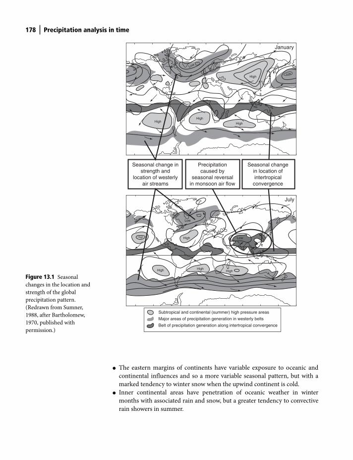
178 Precipitation analysis in time
● The eastern margins of continents have variable exposure to oceanic and
continental influences and so a more variable seasonal pattern, but with a
marked tendency to winter snow when the upwind continent is cold.
● Inner continental areas have penetration of oceanic weather in winter
months with associated rain and snow, but a greater tendency to convective
rain showers in summer.
July
Seasonal change instrength and
location of westerlyair streams
Precipitationcaused by
seasonal reversalin monsoon air flow
Seasonal changein location ofintertropical
convergence
January
High
High
High
HighHighHigh
High
Low
Low
HighHigh
Low
Low
Subtropical and continental (summer) high pressure areas
Major areas of precipitation generation in westerly belts
Belt of precipitation generation along intertropical convergence
Figure 13.1 Seasonal
changes in the location and
strength of the global
precipitation pattern.
(Redrawn from Sumner,
1988, after Bartholomew,
1970, published with
permission.)
Shuttleworth_c13.indd 178Shuttleworth_c13.indd 178 11/3/2011 7:03:09 PM11/3/2011 7:03:09 PM
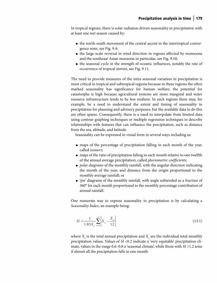
Precipitation analysis in time 179
In tropical regions, there is solar radiation driven seasonality in precipitation with
at least one wet season caused by:
● the north-south movement of the central ascent in the intertropical conver-
gence zone, see Fig. 9.4;
● the large-scale reversal in wind direction in regions affected by monsoons
and the southeast Asian monsoon in particular, see Fig. 9.10;
● the seasonal cycle in the strength of oceanic influences, notably the rate of
occurrence of tropical storms, see Fig. 9.11.
The need to provide measures of the intra-seasonal variation in precipitation is
most critical in tropical and subtropical regions because in these regions the often
marked seasonality has significance for human welfare; the potential for
catastrophe is high because agricultural systems are more marginal and water
resource infrastructure tends to be less resilient. In such regions there may, for
example, be a need to understand the extent and timing of seasonality in
precipitation for planning and advisory purposes, but the available data to do this
are often sparse. Consequently, there is a need to interpolate from limited data
using contour graphing techniques or multiple regression techniques to describe
relationships with features that can influence the precipitation, such as distance
from the sea, altitude, and latitude.
Seasonality can be expressed in visual form in several ways including as:
● maps of the percentage of precipitation falling in each month of the year,
called isomers;
● maps of the ratio of precipitation falling in each month relative to one twelfth
of the annual average precipitation, called pluviometric coefficients;
● polar diagrams of the monthly rainfall, with the angular direction indicating
the month of the year, and distance from the origin proportional to the
monthly average rainfall; or
● ‘pie’ diagrams of the monthly rainfall, with angle subtended as a fraction of
360° for each month proportional to the monthly percentage contribution of
annual rainfall.
One numerate way to express seasonality in precipitation is by calculating a
Seasonality Index, an example being:
12
1
1
1.83 12a
nna
XSI X
X =
= −∑ (13.1)
where Xa is the total annual precipitation and X
n are the individual total monthly
precipitation values. Values of SI <0.2 indicate a ‘very equitable’ precipitation cli-
mate, values in the range 0.6–0.8 a ‘seasonal climate’, while those with SI >1.2 arise
if almost all the precipitation falls in one month.
Shuttleworth_c13.indd 179Shuttleworth_c13.indd 179 11/3/2011 7:03:09 PM11/3/2011 7:03:09 PM
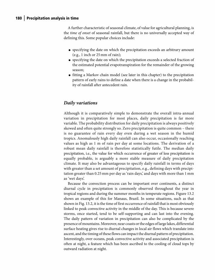
180 Precipitation analysis in time
A further characteristic of seasonal climate, of value for agricultural planning, is
the time of onset of seasonal rainfall, but there is no universally accepted way of
defining this. Some popular choices include:
● specifying the date on which the precipitation exceeds an arbitrary amount
(e.g., 1 inch or 25 mm of rain);
● specifying the date on which the precipitation exceeds a selected fraction of
the estimated potential evapotranspiration for the remainder of the growing
season;
● fitting a Markov chain model (see later in this chapter) to the precipitation
pattern of early rains to define a date when there is a change in the probabil-
ity of rainfall after antecedent rain.
Daily variations
Although it is comparatively simple to demonstrate the overall intra-annual
variation in precipitation for most places, daily precipitation is far more
variable. The probability distribution for daily precipitation is always positively
skewed and often quite strongly so. Zero precipitation is quite common – there
is no guarantee of rain every day even during a wet season in the humid
tropics. Anomalously high daily rainfall can also occur, occasionally reaching
values as high as 1 m of rain per day at some locations. The derivation of a
robust mean daily rainfall is therefore statistically futile. The median daily
precipitation, i.e., the value for which occurrence of greater of less precipitation is
equally probable, is arguably a more stable measure of daily precipitation
climate. It may also be advantageous to specify daily rainfall in terms of days
with greater than a set amount of precipitation, e.g., defining days with precipi-
tation greater than 0.25 mm per day as ‘rain days,’ and days with more than 1 mm
as ‘wet days’.
Because the convection process can be important over continents, a distinct
diurnal cycle in precipitation is commonly observed throughout the year in
tropical regions and during the summer months in temperate regions. Figure 13.2
shows an example of this for Manaus, Brazil. In some situations, such as that
shown in Fig. 13.2, it is the time of first occurrence of rainfall that is most obviously
linked to peak convective activity in the middle of the day. This is because severe
storms, once started, tend to be self-supporting and can last into the evening.
The daily pattern of variation in precipitation can also be complicated by the
presence of mountains. Moreover, near coasts or the edges of large lakes, differential
surface heating gives rise to diurnal changes in local air flows which translate into
ascent, and the timing of these flows can impact the diurnal pattern of precipitation.
Interestingly, over oceans, peak convective activity and associated precipitation is
often at night, a feature which has been ascribed to the cooling of cloud tops by
outward radiation at night.
Shuttleworth_c13.indd 180Shuttleworth_c13.indd 180 11/3/2011 7:03:10 PM11/3/2011 7:03:10 PM
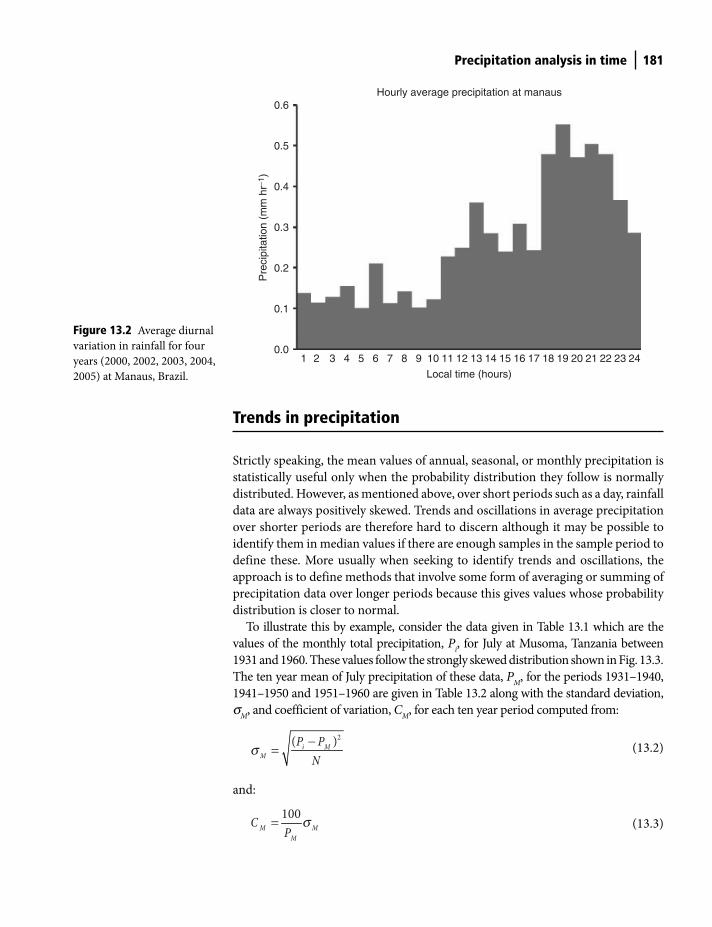
Precipitation analysis in time 181
Trends in precipitation
Strictly speaking, the mean values of annual, seasonal, or monthly precipitation is
statistically useful only when the probability distribution they follow is normally
distributed. However, as mentioned above, over short periods such as a day, rainfall
data are always positively skewed. Trends and oscillations in average precipitation
over shorter periods are therefore hard to discern although it may be possible to
identify them in median values if there are enough samples in the sample period to
define these. More usually when seeking to identify trends and oscillations, the
approach is to define methods that involve some form of averaging or summing of
precipitation data over longer periods because this gives values whose probability
distribution is closer to normal.
To illustrate this by example, consider the data given in Table 13.1 which are the
values of the monthly total precipitation, Pi, for July at Musoma, Tanzania between
1931 and 1960. These values follow the strongly skewed distribution shown in Fig. 13.3.
The ten year mean of July precipitation of these data, PM
, for the periods 1931–1940,
1941–1950 and 1951–1960 are given in Table 13.2 along with the standard deviation,
sM
, and coefficient of variation, CM
, for each ten year period computed from:
2( )i MM
P PN
−=s (13.2)
and:
100M M
M
CP
= s (13.3)
0.01 2 3 4 5 6 7 8 9 10 11 12 13 14 15 16 17
Local time (hours)
Hourly average precipitation at manaus
Pre
cipi
tatio
n (m
m h
r−1 )
18 19 20 21 22 23 24
0.1
0.2
0.3
0.4
0.5
0.6
Figure 13.2 Average diurnal
variation in rainfall for four
years (2000, 2002, 2003, 2004,
2005) at Manaus, Brazil.
Shuttleworth_c13.indd 181Shuttleworth_c13.indd 181 11/3/2011 7:03:10 PM11/3/2011 7:03:10 PM
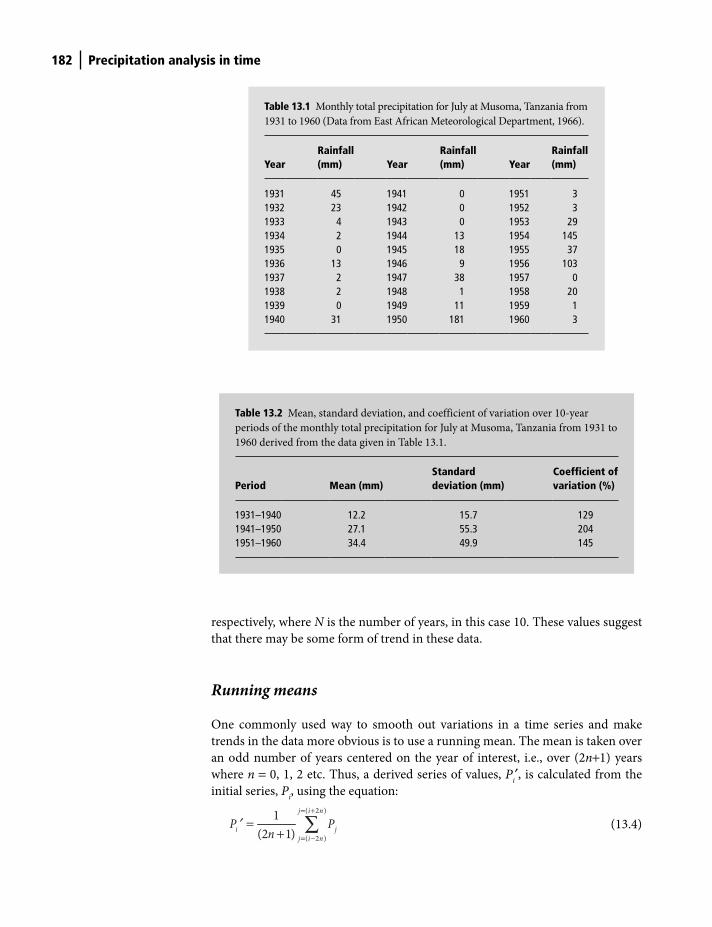
182 Precipitation analysis in time
respectively, where N is the number of years, in this case 10. These values suggest
that there may be some form of trend in these data.
Running means
One commonly used way to smooth out variations in a time series and make
trends in the data more obvious is to use a running mean. The mean is taken over
an odd number of years centered on the year of interest, i.e., over (2n+1) years
where n = 0, 1, 2 etc. Thus, a derived series of values, Pi′, is calculated from the
initial series, Pi, using the equation:
( 2 )
( 2 )
1
(2 1)
j i n
i jj i n
P Pn
= +
= −
=+ ∑¢ (13.4)
Table 13.1 Monthly total precipitation for July at Musoma, Tanzania from
1931 to 1960 (Data from East African Meteorological Department, 1966).
Year Rainfall (mm) Year
Rainfall (mm) Year
Rainfall (mm)
1931 45 1941 0 1951 31932 23 1942 0 1952 31933 4 1943 0 1953 291934 2 1944 13 1954 1451935 0 1945 18 1955 371936 13 1946 9 1956 1031937 2 1947 38 1957 01938 2 1948 1 1958 201939 0 1949 11 1959 11940 31 1950 181 1960 3
Table 13.2 Mean, standard deviation, and coefficient of variation over 10-year
periods of the monthly total precipitation for July at Musoma, Tanzania from 1931 to
1960 derived from the data given in Table 13.1.
Period Mean (mm) Standard deviation (mm)
Coefficient of variation (%)
1931–1940 12.2 15.7 1291941–1950 27.1 55.3 2041951–1960 34.4 49.9 145
Shuttleworth_c13.indd 182Shuttleworth_c13.indd 182 11/3/2011 7:03:13 PM11/3/2011 7:03:13 PM

Precipitation analysis in time 183
This series is valid for values of i in the range (n+1) to (N–n-1), where N is the
number of data elements in the original time series. Figure 13.4a shows the time
series of values of total July precipitation at Musuma, Tanzania and Fig. 13.4b the
time series of the 5-year running average value of these same data. The year-to-
year fluctuations in Fig. 13.4b are much smoother than in Fig. 13.4a, and a trend
toward a wetter period during the 1950s clearly emerges.
Cumulative deviations
Significant and sustained shifts in precipitation can be demonstrated by accumu-
lating the deviations in yearly precipitation about the period mean. Yearly devia-
tions above (positive) or below (negative) the period mean are accumulated
through the data period, either as absolute amounts or as percentages of the mean
precipitation. A plot is then made as a function of time of the accumulated devia-
tions, Pj,a
, or the accumulated percentage residuals, Pj,p
, given by:
,1
( )j
j a ii
P P P=
= −∑ (13.5)
and:
,1
100( )
j
j p ii
P P PP =
= −∑ (13.6)
where Pi are the time series of precipitation undergoing analysis and P is the
mean precipitation for the period of interest. Figure 13.5 shows the results of a
cumulative percentage analysis for annual precipitation at several tropical sites
00
5
Fre
quen
cy o
f rai
nfal
l
10
15
20
10 20 30 40 50 60 70 80
Monthly rainfall (mm)
90 100 110 120 130 140 150 160 170 180 190
Figure 13.3 Frequency
distribution for the July
precipitation at Musoma,
Tanzania from 1931 to 1960
given in Table 13.1.
Shuttleworth_c13.indd 183Shuttleworth_c13.indd 183 11/3/2011 7:03:14 PM11/3/2011 7:03:14 PM
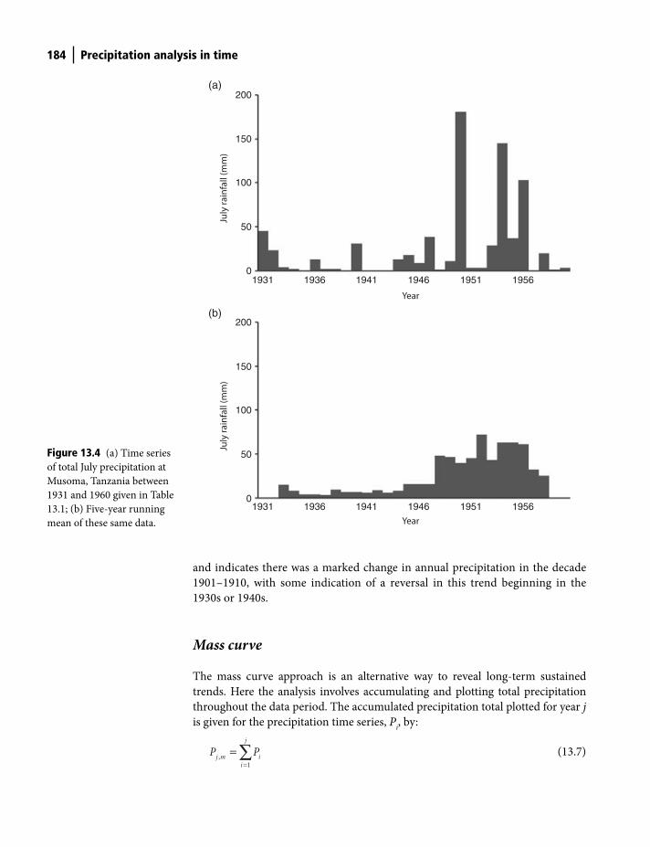
184 Precipitation analysis in time
and indicates there was a marked change in annual precipitation in the decade
1901–1910, with some indication of a reversal in this trend beginning in the
1930s or 1940s.
Mass curve
The mass curve approach is an alternative way to reveal long-term sustained
trends. Here the analysis involves accumulating and plotting total precipitation
throughout the data period. The accumulated precipitation total plotted for year j
is given for the precipitation time series, Pi, by:
,1
j
j m ii
P P=
= ∑ (13.7)
01931 1936 1941 1946
Year
(a)
1951 1956
50Ju
ly ra
infa
ll (m
m)
100
150
200
01931 1936 1941 1946
Year
(b)
1951 1956
50
July
rain
fall
(mm
)
100
150
200
Figure 13.4 (a) Time series
of total July precipitation at
Musoma, Tanzania between
1931 and 1960 given in Table
13.1; (b) Five-year running
mean of these same data.
Shuttleworth_c13.indd 184Shuttleworth_c13.indd 184 11/3/2011 7:03:17 PM11/3/2011 7:03:17 PM
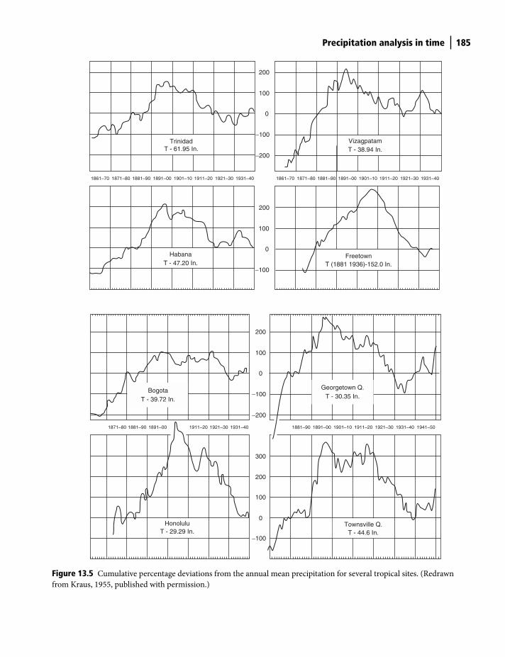
Precipitation analysis in time 185
Freetown
Vizagpatam
HabanaT - 47.20 In.
TrinidadT - 61.95 In. T - 38.94 In.
T (1881 1936)-152.0 In.
−100
100
200
300
0
−200
−100
100
200
0
−200
−100
100
200
0
−100
100
200
0
BogotaT - 39.72 In.
Georgetown Q.T - 30.35 In.
HonoluluT - 29.29 In.
Townsville Q.T - 44.6 In.
1861–70 1871–80 1881–90 1891–00 1901–10 1911–20 1921–30 1931–40 1861–70 1871–80 1881–90 1891–00 1901–10 1911–20 1921–30 1931–40
1871–80 1881–90 1891–00 1911–20 1921–30 1931–40 1881–90 1891–00 1901–10 1911–20 1921–30 1931–40 1941–50
Figure 13.5 Cumulative percentage deviations from the annual mean precipitation for several tropical sites. (Redrawn
from Kraus, 1955, published with permission.)
Shuttleworth_c13.indd 185Shuttleworth_c13.indd 185 11/3/2011 7:03:18 PM11/3/2011 7:03:18 PM
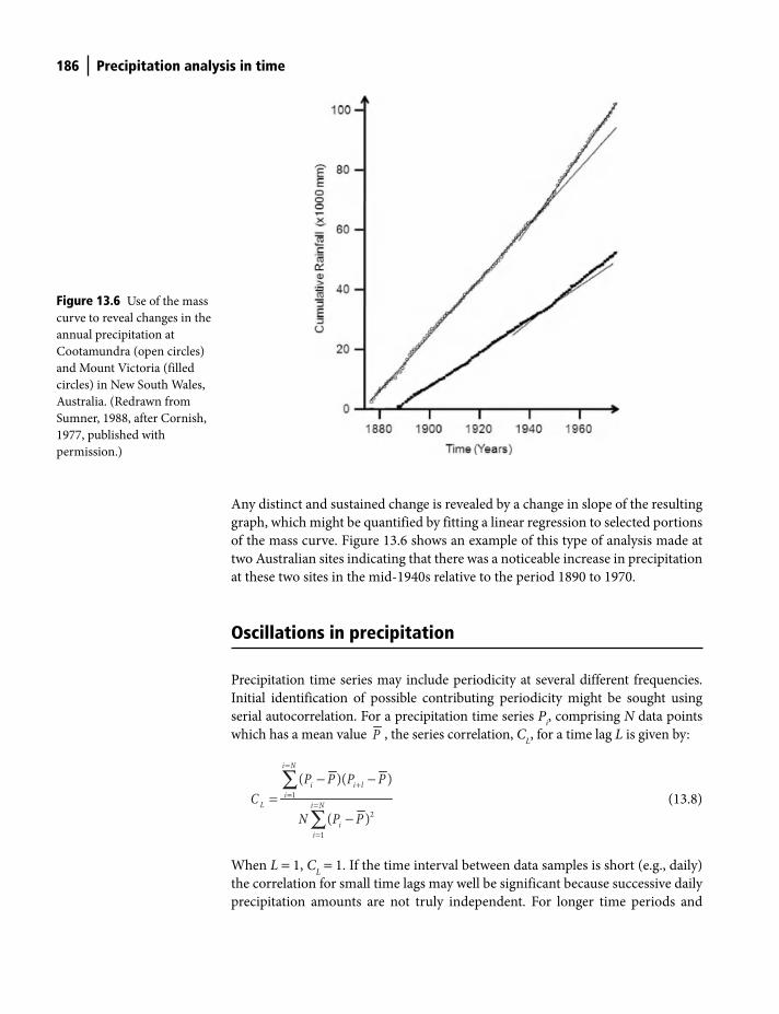
186 Precipitation analysis in time
Any distinct and sustained change is revealed by a change in slope of the resulting
graph, which might be quantified by fitting a linear regression to selected portions
of the mass curve. Figure 13.6 shows an example of this type of analysis made at
two Australian sites indicating that there was a noticeable increase in precipitation
at these two sites in the mid-1940s relative to the period 1890 to 1970.
Oscillations in precipitation
Precipitation time series may include periodicity at several different frequencies.
Initial identification of possible contributing periodicity might be sought using
serial autocorrelation. For a precipitation time series Pi, comprising N data points
which has a mean value P , the series correlation, CL, for a time lag L is given by:
1
2
1
( )( )
( )
i N
i i li
L i N
ii
P P P PC
N P P
=
+=
=
=
− −=
−
∑
∑ (13.8)
When L = 1, CL = 1. If the time interval between data samples is short (e.g., daily)
the correlation for small time lags may well be significant because successive daily
precipitation amounts are not truly independent. For longer time periods and
Figure 13.6 Use of the mass
curve to reveal changes in the
annual precipitation at
Cootamundra (open circles)
and Mount Victoria (filled
circles) in New South Wales,
Australia. (Redrawn from
Sumner, 1988, after Cornish,
1977, published with
permission.)
Shuttleworth_c13.indd 186Shuttleworth_c13.indd 186 11/3/2011 7:03:18 PM11/3/2011 7:03:18 PM
Precipitation analysis in time 187
longer sample periods, there will likely be a progressive and marked decrease in CL
with increasing time lags. However, if there is periodicity present in the data series,
the magnitude of the correlation coefficient will increase again for a time lag that
matches the period of one of the fluctuations present. A graph of serial correlation
coefficient versus time lag is called the correlogram.
Identification of periodicity in a precipitation time series can also be made using
harmonic (Fourier) analysis. This entails fitting a mathematical function P f of time
t (in units appropriate to the problem) to a time series with the general form:
1
( ) cos( )k n
fk k
kP t P P kt
=
=
= + −∑ f (13.9)
where Pk and f
k are the amplitude and phase assigned to the k th harmonic in the
harmonic series so that it adequately represents P f. The maximum value of n is
determined by the requirement that there is at least one full sinusoidal cycle of the
corresponding term in the time period for which data are available. An earlier
autocorrelation analysis might be used to guide the selection of terms in Equation
(13.8) for which fitting is made. The contribution of each harmonic term to the
total variance is subsequently found by expressing the variance for each harmonic
as a proportion of the total variance. Not every harmonic term in the series can
necessarily be associated with an identifiable physical mechanism.
As an alternative to harmonic analysis, numerical filters can be applied to the
precipitation time series to identify and enhance the contributions from influences
with different periodicity. Figure 13.7 shows an example of this approach in which
digital filters are used to identify fluctuating contributions superimposed on the
moving average value, in this figure corresponding to periodicity between 6 and 8
years, between 8 and 13 years and between 13 and 30 years. There is a possible
association with the sunspot cycle when the 8 to 13 year filter is applied to these
data, with the northern hemisphere (as represented by the west coast of the USA)
out of phase with the southern hemisphere (as represented by the east coast of
Australia). There is also some suggestion of association with the 18 year lunar
cycle revealed by applying the 13–30 year filter. Once trends and fluctuations in
observed precipitation records have been clearly established, they might be
extrapolated into the future for forecast purposes.
System signatures
The variation with time of precipitation intensity within a precipitation event is
called the system signature of the storm that gave rise to the precipitation. As might
be expected from the discussion given in Chapter 11, there is an important
distinction between convective and synoptic-scale storms. Observations of
precipitation rate during storms indicates that not only do most large-scale
synoptic systems produce longer duration and lower intensity precipitation than
convective storms, but also the distribution of precipitation intensity through the
Shuttleworth_c13.indd 187Shuttleworth_c13.indd 187 11/3/2011 7:03:20 PM11/3/2011 7:03:20 PM
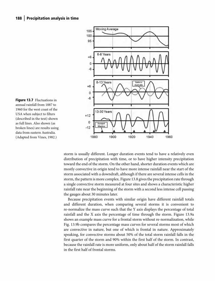
188 Precipitation analysis in time
storm is usually different. Longer duration events tend to have a relatively even
distribution of precipitation with time, or to have higher intensity precipitation
toward the end of the storm. On the other hand, shorter duration events which are
mostly convective in origin tend to have more intense rainfall near the start of the
storm associated with a downdraft, although if there are several intense cells in the
storm, the pattern is more complex. Figure 13.8 gives the precipitation rate through
a single convective storm measured at four sites and shows a characteristic higher
rainfall rate near the beginning of the storm with a second less intense cell passing
the gauges about 30 minutes later.
Because precipitation events with similar origin have different rainfall totals
and different duration, when comparing several storms it is convenient to
re-normalize the mass curve such that the Y axis displays the percentage of total
rainfall and the X axis the percentage of time through the storm. Figure 13.9a
shows an example mass curve for a frontal storm without re-normalization, while
Fig. 13.9b compares the percentage mass curves for several storms most of which
are convective in nature, but one of which is frontal in nature. Approximately
speaking, for convective storms about 50% of the total storm rainfall falls in the
first quarter of the storm and 90% within the first half of the storm. In contrast,
because the rainfall rate is more uniform, only about half of the storm rainfall falls
in the first half of frontal storms.
Figure 13.7 Fluctuations in
annual rainfall from 1887 to
1960 for the west coast of the
USA when subject to filters
(described in the text) shown
as full lines. Also shown (as
broken lines) are results using
data from eastern Australia.
(Adapted from Vines, 1982.)
Shuttleworth_c13.indd 188Shuttleworth_c13.indd 188 11/3/2011 7:03:21 PM11/3/2011 7:03:21 PM
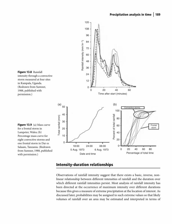
Precipitation analysis in time 189
Intensity-duration relationships
Observations of rainfall intensity suggest that there exists a basic, inverse, non-
linear relationship between different intensities of rainfall and the duration over
which different rainfall intensities persist. Most analysis of rainfall intensity has
been directed at the occurrence of maximum intensity over different durations
because this gives a measure of extreme precipitation at the location of interest. As
discussed later, probabilities may be assigned to such extreme values so that likely
volumes of rainfall over an area may be estimated and interpreted in terms of
00
12
24
36
48
60
72
84
96
108
120
20Time after start (minutes)
Rai
nfal
l int
ensi
ty (
mm
hr−
1 )
40 60
Figure 13.8 Rainfall
intensity through a convective
storm measured at four sites
in Kampala, Uganda.
(Redrawn from Sumner,
1988, published with
permission.)
018:00 24:00
5 Aug. 1973 6 Aug. 197306:00
Tot
al r
ainf
all (
mm
)
10
Date and time
20
30
40
50(a) (b)
00 20 40 60 80
Percentage of total time
Frontalstorm
Convective storms
Per
cent
of t
otal
rai
nfal
l
20
40
60
80
100
Figure 13.9 (a) Mass curve
for a frontal storm in
Lampeter, Wales; (b)
Percentage mass curve for
eight convective storms and
one frontal storm in Dar es
Salaam, Tanzania. (Redrawn
from Sumner, 1988, published
with permission.)
Shuttleworth_c13.indd 189Shuttleworth_c13.indd 189 11/3/2011 7:03:21 PM11/3/2011 7:03:21 PM
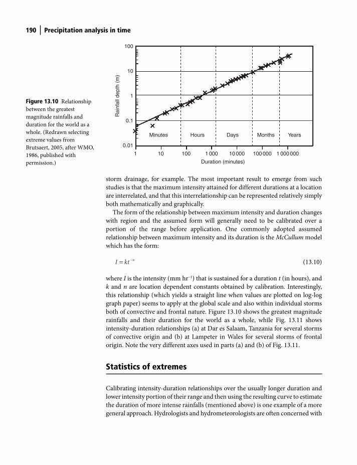
190 Precipitation analysis in time
storm drainage, for example. The most important result to emerge from such
studies is that the maximum intensity attained for different durations at a location
are interrelated, and that this interrelationship can be represented relatively simply
both mathematically and graphically.
The form of the relationship between maximum intensity and duration changes
with region and the assumed form will generally need to be calibrated over a
portion of the range before application. One commonly adopted assumed
relationship between maximum intensity and its duration is the McCullum model
which has the form:
nI kt −= (13.10)
where I is the intensity (mm hr−1) that is sustained for a duration t (in hours), and
k and n are location dependent constants obtained by calibration. Interestingly,
this relationship (which yields a straight line when values are plotted on log-log
graph paper) seems to apply at the global scale and also within individual storms
both of convective and frontal nature. Figure 13.10 shows the greatest magnitude
rainfalls and their duration for the world as a whole, while Fig. 13.11 shows
intensity-duration relationships (a) at Dar es Salaam, Tanzania for several storms
of convective origin and (b) at Lampeter in Wales for several storms of frontal
origin. Note the very different axes used in parts (a) and (b) of Fig. 13.11.
Statistics of extremes
Calibrating intensity-duration relationships over the usually longer duration and
lower intensity portion of their range and then using the resulting curve to estimate
the duration of more intense rainfalls (mentioned above) is one example of a more
general approach. Hydrologists and hydrometeorologists are often concerned with
1
0.01
0.1
1
10
100
10
Rai
nfal
l dep
th (
m)
100 1 000
Duration (minutes)
Minutes Hours Days Months Years
10 000 100 000 1 000 000
Figure 13.10 Relationship
between the greatest
magnitude rainfalls and
duration for the world as a
whole. (Redrawn selecting
extreme values from
Brutsaert, 2005, after WMO,
1986, published with
permission.)
Shuttleworth_c13.indd 190Shuttleworth_c13.indd 190 11/3/2011 7:03:22 PM11/3/2011 7:03:22 PM
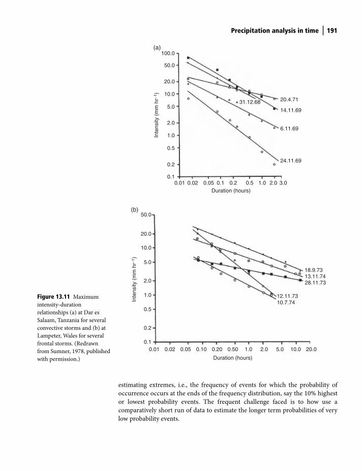
Precipitation analysis in time 191
estimating extremes, i.e., the frequency of events for which the probability of
occurrence occurs at the ends of the frequency distribution, say the 10% highest
or lowest probability events. The frequent challenge faced is to how use a
comparatively short run of data to estimate the longer term probabilities of very
low probability events.
0.010.1
0.2
0.5
1.0
2.0
5.0
10.0
20.0
50.0
100.0
0.02 0.05 0.1 0.2Duration (hours)
Inte
nsity
(m
m h
r−1 )
0.5 1.0 2.0 3.0
31.12.68 20.4.71
14.11.69
24.11.69
6.11.69
(a)
0.1
0.2
0.5
1.0
2.0
5.0
10.0
20.0
50.0
Inte
nsity
(m
m h
r−1 )
Duration (hours)
18.9.73
28.11.73
12.11.7310.7.74
13.11.74
0.01 0.02 0.05 0.10 0.20 0.50 1.0 2.0 5.0 10.0 20.0
(b)
Figure 13.11 Maximum
intensity-duration
relationships (a) at Dar es
Salaam, Tanzania for several
convective storms and (b) at
Lampeter, Wales for several
frontal storms. (Redrawn
from Sumner, 1978, published
with permission.)
Shuttleworth_c13.indd 191Shuttleworth_c13.indd 191 11/3/2011 7:03:23 PM11/3/2011 7:03:23 PM
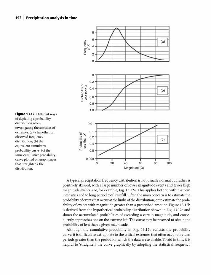
192 Precipitation analysis in time
A typical precipitation frequency distribution is not usually normal but rather is
positively skewed, with a large number of lower magnitude events and fewer high
magnitude events, see, for example, Fig. 13.12a. This applies both to within-storm
intensities and to long period total rainfall. Often the main concern is to estimate the
probability of events that occur at the limbs of the distribution, or to estimate the prob-
ability of events with magnitude greater than a prescribed amount. Figure 13.12b
is derived from the hypothetical probability distribution shown in Fig. 13.12a and
shows the accumulated probabilities of exceeding a certain magnitude, and conse-
quently approaches one on the extreme left. The curve may be reversed to obtain the
probability of less than a given magnitude.
Although the cumulative probability in Fig. 13.12b reflects the probability
curve, it is difficult to extrapolate to the critical extremes that often occur at return
periods greater than the period for which the data are available. To aid in this, it is
helpful to ‘straighten’ the curve graphically by adopting the statistical frequency
00.999
0.8
0.4
0.2
0.1
0.01
1.0
0.8
0.6
0.4
0.2
0
0
2
4
6
8
20 40 60 80 100
Magnitude (X)
(c)
(b)
(a)
Pro
babi
lity
ofle
ss th
an X
Pro
babi
lity
ofle
ss th
an X
Fre
quen
cyof
X
Figure 13.12 Different ways
of depicting a probability
distribution when
investigating the statistics of
extremes: (a) a hypothetical
observed frequency
distribution; (b) the
equivalent cumulative
probability curve; (c) the
same cumulative probability
curve plotted on graph paper
that ‘straightens’ the
distribution.
Shuttleworth_c13.indd 192Shuttleworth_c13.indd 192 11/3/2011 7:03:24 PM11/3/2011 7:03:24 PM
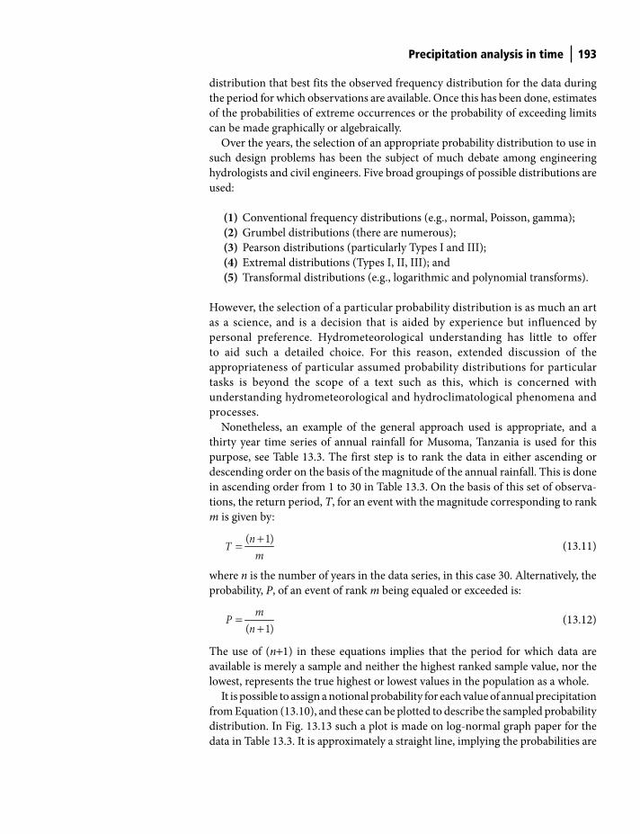
Precipitation analysis in time 193
distribution that best fits the observed frequency distribution for the data during
the period for which observations are available. Once this has been done, estimates
of the probabilities of extreme occurrences or the probability of exceeding limits
can be made graphically or algebraically.
Over the years, the selection of an appropriate probability distribution to use in
such design problems has been the subject of much debate among engineering
hydrologists and civil engineers. Five broad groupings of possible distributions are
used:
(1) Conventional frequency distributions (e.g., normal, Poisson, gamma);
(2) Grumbel distributions (there are numerous);
(3) Pearson distributions (particularly Types I and III);
(4) Extremal distributions (Types I, II, III); and
(5) Transformal distributions (e.g., logarithmic and polynomial transforms).
However, the selection of a particular probability distribution is as much an art
as a science, and is a decision that is aided by experience but influenced by
personal preference. Hydrometeorological understanding has little to offer
to aid such a detailed choice. For this reason, extended discussion of the
appropriateness of particular assumed probability distributions for particular
tasks is beyond the scope of a text such as this, which is concerned with
understanding hydrometeorological and hydroclimatological phenomena and
processes.
Nonetheless, an example of the general approach used is appropriate, and a
thirty year time series of annual rainfall for Musoma, Tanzania is used for this
purpose, see Table 13.3. The first step is to rank the data in either ascending or
descending order on the basis of the magnitude of the annual rainfall. This is done
in ascending order from 1 to 30 in Table 13.3. On the basis of this set of observa-
tions, the return period, T, for an event with the magnitude corresponding to rank
m is given by:
( 1)nTm+= (13.11)
where n is the number of years in the data series, in this case 30. Alternatively, the
probability, P, of an event of rank m being equaled or exceeded is:
( 1)
mPn
=+
(13.12)
The use of (n+1) in these equations implies that the period for which data are
available is merely a sample and neither the highest ranked sample value, nor the
lowest, represents the true highest or lowest values in the population as a whole.
It is possible to assign a notional probability for each value of annual precipitation
from Equation (13.10), and these can be plotted to describe the sampled probability
distribution. In Fig. 13.13 such a plot is made on log-normal graph paper for the
data in Table 13.3. It is approximately a straight line, implying the probabilities are
Shuttleworth_c13.indd 193Shuttleworth_c13.indd 193 11/3/2011 7:03:24 PM11/3/2011 7:03:24 PM
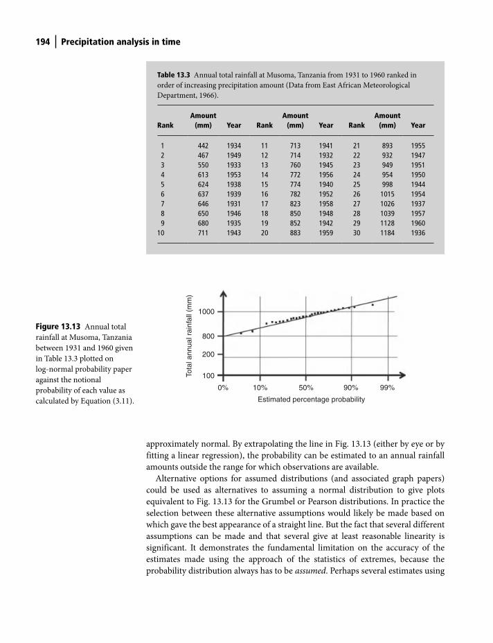
194 Precipitation analysis in time
approximately normal. By extrapolating the line in Fig. 13.13 (either by eye or by
fitting a linear regression), the probability can be estimated to an annual rainfall
amounts outside the range for which observations are available.
Alternative options for assumed distributions (and associated graph papers)
could be used as alternatives to assuming a normal distribution to give plots
equivalent to Fig. 13.13 for the Grumbel or Pearson distributions. In practice the
selection between these alternative assumptions would likely be made based on
which gave the best appearance of a straight line. But the fact that several different
assumptions can be made and that several give at least reasonable linearity is
significant. It demonstrates the fundamental limitation on the accuracy of the
estimates made using the approach of the statistics of extremes, because the
probability distribution always has to be assumed. Perhaps several estimates using
Table 13.3 Annual total rainfall at Musoma, Tanzania from 1931 to 1960 ranked in
order of increasing precipitation amount (Data from East African Meteorological
Department, 1966).
RankAmount
(mm) Year RankAmount
(mm) Year RankAmount
(mm) Year
1 442 1934 11 713 1941 21 893 1955 2 467 1949 12 714 1932 22 932 1947 3 550 1933 13 760 1945 23 949 1951 4 613 1953 14 772 1956 24 954 1950 5 624 1938 15 774 1940 25 998 1944 6 637 1939 16 782 1952 26 1015 1954 7 646 1931 17 823 1958 27 1026 1937 8 650 1946 18 850 1948 28 1039 1957 9 680 1935 19 852 1942 29 1128 196010 711 1943 20 883 1959 30 1184 1936
0% 10%
100
200
800
1000
50%
Estimated percentage probability
Tota
l ann
ual r
ainf
all (
mm
)
90% 99%
Figure 13.13 Annual total
rainfall at Musoma, Tanzania
between 1931 and 1960 given
in Table 13.3 plotted on
log-normal probability paper
against the notional
probability of each value as
calculated by Equation (3.11).
Shuttleworth_c13.indd 194Shuttleworth_c13.indd 194 11/3/2011 7:03:26 PM11/3/2011 7:03:26 PM

Precipitation analysis in time 195
different assumed probability distributions should be made and the mean value
of the resulting ensemble of estimates used, with the range of estimates given
using different assumptions then providing an approximate lowest estimate of the
error implicit in the calculation. An estimated probability given by the statistics
of extremes approach is compromised if the sample of precipitation in the
observational record used is not representative of the precipitation climate at the
location of interest. It also involves the implicit assumption that the precipitation
climate is not changing.
Conditional probabilities
Up to this point the analysis perspective we have adopted has been that precipita-
tion events are independent of each other. In reality, however, precipitation cli-
mates often can be viewed as having ‘wet spells’ and ‘dry spells’. This is evident in
the fact that precipitation data commonly reveal seasonal dependency and some-
times evidence of periodicity. A major cause of shorter term persistence is the fact
that the weather conditions and weather systems involved in the production of
precipitation themselves have some persistence. Indeed, much of the skill in
weather forecasting depends on this fact.
The presence of persistence in the precipitation measured at a particular loca-
tion can be sought, and the extent to which it occurs quantified, using simple
stochastic techniques. A long time series of observed precipitation is analyzed to
count the number of times a ‘wet day’ or ‘rain day’ follows a preceding period
comprising a specified number of days with rain or a specified number of days
without rain. In this way a set of conditional probabilities are derived that charac-
terize the level of persistence in the data record. Figure 13.14 shows a simple exam-
ple. In this case the probability that a wet period will be further extended by a day
with rain, or a dry period further extended by a day without rain is plotted for
Selangor, Malaysia.
The probabilities shown in Fig. 13.13 are examples of conditional probabilities,
in this case for daily rainfall. The four relevant basic conditional probabilities are
the probability that day n is wet if day (n−1) was wet; the probability that day n is
wet if day (n−1) was dry; the probability that day n is dry if day (n−1) was dry; and
the probability that day n is dry if day (n−1) was wet. Such conditional probabili-
ties (or those of greater complexity) are the basis of a widely used mathematical
model of persistence, the Markov chain. This model, whose detailed description is
beyond the scope of this text, begins by calculating a number of equations derived
to calculate the probability of a wet day or days after a wet or a dry day, of wet or
dry spells of different lengths, etc. One important application of models of persis-
tence such as the Markov chain model is to generate synthetic time series of pre-
cipitation which have the same level of persistence as the data series originally
used to calibrate the model. Such long time series might be used in design studies
for hydraulic structures.
Shuttleworth_c13.indd 195Shuttleworth_c13.indd 195 11/3/2011 7:03:26 PM11/3/2011 7:03:26 PM
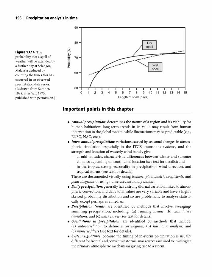
196 Precipitation analysis in time
Important points in this chapter
● Annual precipitation: determines the nature of a region and its viability for
human habitation: long-term trends in its value may result from human
intervention in the global system, while fluctuations may be predictable (e.g.,
ENSO, NAO, etc.).
● Intra-annual precipitation: variations caused by seasonal changes in atmos-
pheric circulation, especially in the ITCZ, monsoons systems, and the
strength and location of westerly wind bands, give:
— at mid-latitudes, characteristic differences between winter and summer
climates depending on continental location (see text for details); and
— in the tropics, strong seasonality in precipitation, wind direction, and
tropical storms (see text for details).
These are documented visually using isomers, pluviometric coefficients, and
polar diagrams or using numerate seasonality indices.
● Daily precipitation: generally has a strong diurnal variation linked to atmos-
pheric convection, and daily total values are very variable and have a highly
skewed probability distribution and so are problematic to analyze statisti-
cally, except perhaps as a median.
● Precipitation trends: are identified by methods that involve averaging/
summing precipitation, including: (a) running means; (b) cumulative
deviations; and (c) mass curves (see text for details).
● Oscillations in precipitation: are identified by methods that include:
(a) autocorrelation to define a correlogram; (b) harmonic analysis; and
(c) numeric filters (see text for details).
● System signatures: because the timing of in-storm precipitation is usually
different for frontal and convective storms, mass curves are used to investigate
the primary atmospheric mechanism giving rise to a storm.
0
50
60
70
80
90
Pro
babi
lity
(%)
1 2 3
Dryspell
Wetspell
4 5 6
Length of spell (days)
7 8 9 10 11 12 13 14 15
Figure 13.14 The
probability that a spell of
weather will be extended by
a further day at Selangor,
Malaysia deduced by
counting the times this has
occurred in an observed
precipitation data series.
(Redrawn from Sumner,
1988, after Yap, 1973,
published with permission.)
Shuttleworth_c13.indd 196Shuttleworth_c13.indd 196 11/3/2011 7:03:26 PM11/3/2011 7:03:26 PM
Precipitation analysis in time 197
● Intensity-duration relationships: observations of rainfall intensity suggest
an inverse non-linear relationship between the maximum intensity, I, of
rainfall and duration, t, over which that intensity persists that applies to
storm totals for regions (and the globe) and within-storm intensity (I = k t−n
is often assumed).
● Statistics of extremes: in hydrological design, the frequency of rare
precipitation events is estimated by fitting an assumed probability distribution
to data records of limited duration, then extrapolating to extreme probabilities
(not sampled) to estimate the likelihood of the event (see text for an example).
● Conditional probabilities: because weather systems have finite lifetimes,
stochastic techniques can be used to calibrate numerical models of day-to-
day persistence in precipitation data records which can then be used to
calculate long synthetic precipitation records that have the same persistence
characteristics.
References
Bartholomew, J.C. (1970) Advanced Atlas of Modern Geography. J.C. Bartholomew,
Edinburgh.
Brutsaert, W. (2005) Hydrology: An Introduction. Cambridge University Press, Cambridge.
Cornish, P.M. (1977) Changes in seasonal and annual rainfall in New South Wales. Search,
8, 38–40.
East African Meteorological Department (1966) Monthly and Annual Rainfall in Tanganyika
and Zanzibar during years 1931 to 1960, East African Meteorological Department,
Nairobi.
Kraus, E.B. (1955) Secular changes in tropical rainfall regimes. Quarterly Journal of the
Royal Meteorological Society, 81, 198–210.
Sumner, G.N. (1978) The prediction of short-duration storm intensity maxima. Journal
of Hydrology, 37, 91–100.
Sumner, G.N. (1988) Precipitation Process and Analysis. John Wiley and Sons, Bath, UK.
Vines, R.G. (1982) Rainfall patterns in the western United States. Journal of Geophysical
Research, 87 (C9), 7303–11.
WMO (1986) Manual for Estimation of Probable Maximum Precipitation. Operational
Hydrology Report No. 1, WMO-No 332, World Meteorological Organization, Geneva.
Yap, O. (1973) The persistence of wet and dry spells in Sungei Buloh, Selangor. Meteorological
Magazine, 102, 240–45.
Shuttleworth_c13.indd 197Shuttleworth_c13.indd 197 11/3/2011 7:03:27 PM11/3/2011 7:03:27 PM
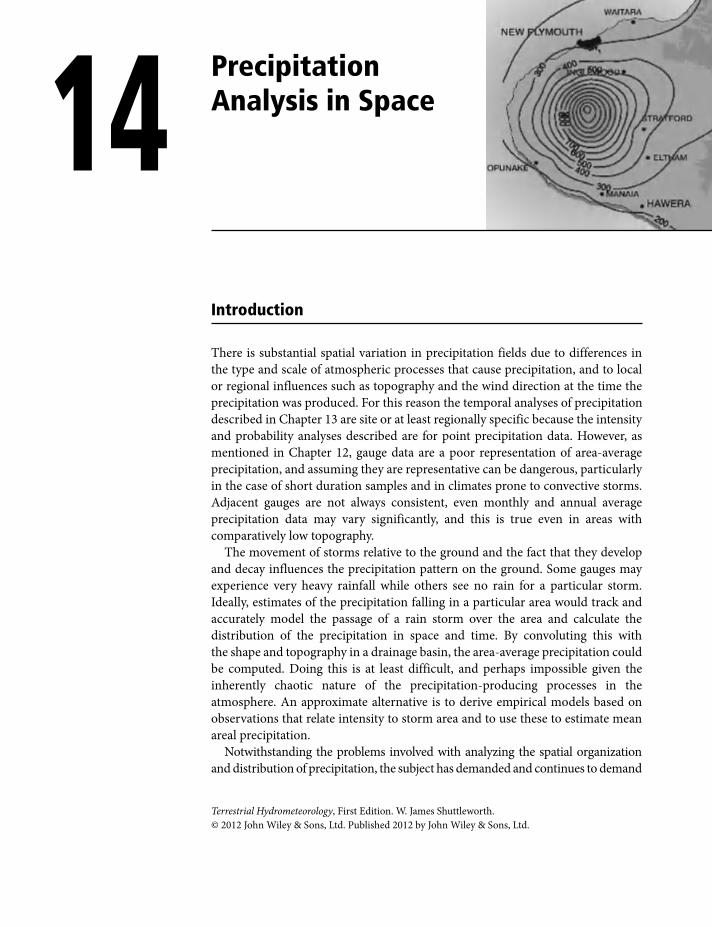
Introduction
There is substantial spatial variation in precipitation fields due to differences in
the type and scale of atmospheric processes that cause precipitation, and to local
or regional influences such as topography and the wind direction at the time the
precipitation was produced. For this reason the temporal analyses of precipitation
described in Chapter 13 are site or at least regionally specific because the intensity
and probability analyses described are for point precipitation data. However, as
mentioned in Chapter 12, gauge data are a poor representation of area-average
precipitation, and assuming they are representative can be dangerous, particularly
in the case of short duration samples and in climates prone to convective storms.
Adjacent gauges are not always consistent, even monthly and annual average
precipitation data may vary significantly, and this is true even in areas with
comparatively low topography.
The movement of storms relative to the ground and the fact that they develop
and decay influences the precipitation pattern on the ground. Some gauges may
experience very heavy rainfall while others see no rain for a particular storm.
Ideally, estimates of the precipitation falling in a particular area would track and
accurately model the passage of a rain storm over the area and calculate the
distribution of the precipitation in space and time. By convoluting this with
the shape and topography in a drainage basin, the area-average precipitation could
be computed. Doing this is at least difficult, and perhaps impossible given the
inherently chaotic nature of the precipitation-producing processes in the
atmosphere. An approximate alternative is to derive empirical models based on
observations that relate intensity to storm area and to use these to estimate mean
areal precipitation.
Notwithstanding the problems involved with analyzing the spatial organization
and distribution of precipitation, the subject has demanded and continues to demand
14 Precipitation Analysis in Space
Terrestrial Hydrometeorology, First Edition. W. James Shuttleworth.
© 2012 John Wiley & Sons, Ltd. Published 2012 by John Wiley & Sons, Ltd.
Shuttleworth_c14.indd 198Shuttleworth_c14.indd 198 11/3/2011 7:02:40 PM11/3/2011 7:02:40 PM

Precipitation Analysis in Space 199
great attention. Not least this is because area-average precipitation is a major influence
on human settlement and development. Understanding the spatial organization of
precipitation is also crucial to hydrologists and civil engineers concerned with the
design of infrastructure. On the one hand, long-term area-average precipitation rates
determine available surface water resources while, on the other hand, short-term
area-average rates are needed when designing flood protection systems.
Mapping precipitation
Mapping precipitation is a straightforward and visually convenient way to illustrate
the organization of precipitation in space. However, precipitation is a meteorological
variable that is difficult to map, especially from gauge data which is the most
common source of the information used, because the point samples available may
be unrepresentative. Because precipitation is so spatially variable, there may be
extreme values which are missed, especially if the gauge network used is sparse
and uneven. There is also likelihood that a network of gauges will mis-sample local
systematic variations in precipitation associated with topography. In principle,
measurements made with radar would not be subject to the same shortcomings
but, as discussed in Chapter 12, the errors associated with radar measurement are
so large that such data only become reliable when re-normalized to an underlying
gauge network. Hence, the problems associated with gauge sampling remain.
Consequently, gauge data remain the basis of precipitation mapping, and for many
parts of the world are likely to remain so for some considerable time.
To use gauges for mapping it is necessary to assume precipitation is a spatially
continuous variable with no dramatic discontinuities, and to assume that it is
adequately sampled by the gauge network used. Correlation tests between gauge
measurements might provide some level of reassurance that a comparatively
smooth field with point to point correlation is being adequately sampled. In
principle the mapping process is then simple. It involves drawing isohyets, i.e.,
lines of constant precipitation, between the point precipitation data available.
Figure 14.1 provides a simple example of the process used.
The accuracy with which isohyets can be drawn will depend on the density of
the gauge network because spurious high or low values can easily dominate the
resulting map if the gauge network is sparse. The assumptions used when drawing
smoothed isohyets also influences accuracy and, if isohyets are drawn manually,
may be subjective. The presence of topography in the area mapped can also affect
accuracy because its influence on precipitation rate is rarely properly sampled and
will therefore be poorly acknowledged in isohyetal maps. However, with knowl-
edge of the underlying topography, a skilled operator or computer program can
make some recognition of the tendency toward higher precipitation at higher
locations when specifying smooth contours of precipitation. In areas with very
strong relief the influence on isohyets of making such allowances for height might
even match the influence of the available gauge data.
Shuttleworth_c14.indd 199Shuttleworth_c14.indd 199 11/3/2011 7:02:42 PM11/3/2011 7:02:42 PM
200 Precipitation Analysis in Space
A commonly encountered issue when preparing isohyet maps is the fact that, as
a result of instrumental or human error, precipitation data is rarely 100% complete.
In the absence of a particular gauge measurement, an estimate of the missing value
is normally made from that measured at nearby gauges. In areas with low relief
the arithmetic mean of the values at three to four nearby stations might be adopted.
However, in areas with high relief a preferable alternative is to take the average of
these station values weighted by the long-term average ratio between stations.
Areal mean precipitation
Estimates of area-average precipitation from gauge network data are a focus of interest
within hydrology because they provide the basis for water resource estimation or
extreme event (flood or drought) forecasting. The estimate required is the total
volume of water falling on a specific drainage basin, i.e., the area of the basin multiplied
by the area-average precipitation depth. In areas with low relief where there is an even
distribution of gauges, a simple arithmetic average will provide an adequate estimate.
However, such conditions are rarely met and one of several alternative ways of taking
a weighted mean of the gauge measurements available is required. Weights can be
assigned in two general ways, either using mapping methods that involve or are
equivalent to drawing isohyets (including the computational equivalents such as
kriging techniques or reciprocal-distance-squared methods), or geometric methods
such as the Triangle method or Theissen method in which areas are defined over
which precipitation is assumed uniform. In practice, studies suggest that these
methods tend to produce comparable results especially if applied over a long period.
Isohyetal method
The basis of this method is straightforward, it involves:
(1) constructing isohyets across the catchment based on measured values,
including making allowance for relief if appropriate;
Figure 14.1 The process of
drawing isohyets from gauge
data which involves
estimating the location of
points with the required value
between pairs of gauge
measurements then drawing
smoothed isohyets from
these.
10 mm 12 mm 11mm
8 mm
Trueinformation
9 mm
7 mm
Smoothedisohyet
(subjective, or subjectto assumption)
Shuttleworth_c14.indd 200Shuttleworth_c14.indd 200 11/3/2011 7:02:42 PM11/3/2011 7:02:42 PM
Precipitation Analysis in Space 201
(2) measuring or computing the area between isohyets to provide the weights
to be used when calculating the average value; and
(3) creating the weighted average by adding the products of the area between
isohyets in the catchment with the mean precipitation between isohyets.
Figure 14.2 illustrates the approach used in the Isohyetal method for an example
catchment. Using this method with these data and this example catchment,
Sumner (1988) calculated a catchment average precipitation of 17.3 mm.
Computer calculations of mean rainfall over selected catchments based on
mapping can also be made using kriging methods or the simpler (but arguably as
effective) Reciprocal-Distance-Squared method, both of which are similar in
concept to the Isohyetal method. In the Reciprocal-Distance-Squared method, a
value of precipitation, Pi (in mm), is assigned to each area element in the catchment
into which the catchment is subdivided by the computer program. This value is
the average of the nearest three gauges weighted by the square of the inverse
distances, d1, d
2, and d
3 (in m) between the element and the three gauges (Fig. 14.3).
Thus Pi is calculated from:
2 2 2
1 1 2 2 3 3
2 2 2
1 2 3
( ) ( ) ( )
( ) ( ) ( )i
P d P d P dP
d d d
− − −
− − −
+ +=
+ +
(14.1)
Figure 14.2 Calculation of area-average precipitation using the Isohyetal Method. (From Sumner, 1988, published with
permission.)
10
Basin margin
Contours
Isohyets (mm)
Point values (mm)
15 20
14.9
12.7
27.2
25
26.1
19.0
27.326.5
25.8
24.2
10.89.2
5.610
7.1
5
5
10 15
15.0
2018.5
25
7.14.7
Shuttleworth_c14.indd 201Shuttleworth_c14.indd 201 11/3/2011 7:02:42 PM11/3/2011 7:02:42 PM
202 Precipitation Analysis in Space
Triangle method
This method involves:
(1) constructing a network of triangles as near equilateral as possible, with one
of the available gauges at the apex of each triangle;
(2) measuring or computing the area of each triangle or portion of each trian-
gle that is within the basin to provide the weights to be used when calculat-
ing the average value;
(3) if needed, making a ‘best guess’ of the precipitation for any area of the
catchment not included in a triangle; and
(4) calculating the weighted average by adding the products of the area of each
triangle with the mean precipitation for the three gauges at the apex of
each triangle.
Figure 14.4 illustrates the approach used in the Triangle Method for an example
catchment. Using this method with these data and this example catchment,
Sumner (1988) calculated a catchment average precipitation of 17.8 mm.
Theissen method
The Theissen method is often the preferred method for estimating area-average
precipitation. The method involves:
(1) constructing a network of polygons by drawing the perpendicular bisector
of the line joining each pair of gauges;
Figure 14.3 Calculating
area-average precipitation
using the reciprocal-
distance-squared method.
(Precipitation P1, P
2, and P
3
in mm, distance d1, d
2, and
d3 in m.)
P1P2
d1 d2
d3
P3
Shuttleworth_c14.indd 202Shuttleworth_c14.indd 202 11/3/2011 7:02:44 PM11/3/2011 7:02:44 PM
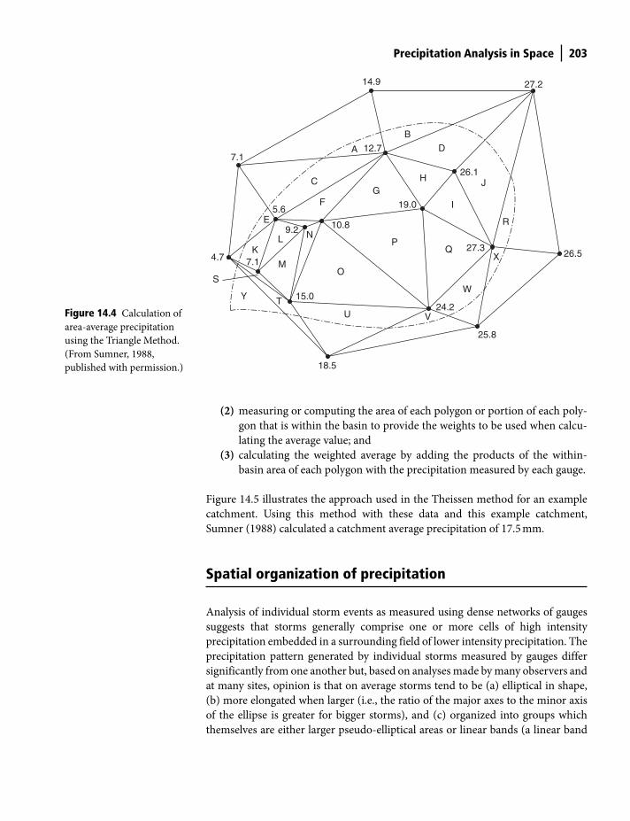
Precipitation Analysis in Space 203
(2) measuring or computing the area of each polygon or portion of each poly-
gon that is within the basin to provide the weights to be used when calcu-
lating the average value; and
(3) calculating the weighted average by adding the products of the within-
basin area of each polygon with the precipitation measured by each gauge.
Figure 14.5 illustrates the approach used in the Theissen method for an example
catchment. Using this method with these data and this example catchment,
Sumner (1988) calculated a catchment average precipitation of 17.5 mm.
Spatial organization of precipitation
Analysis of individual storm events as measured using dense networks of gauges
suggests that storms generally comprise one or more cells of high intensity
precipitation embedded in a surrounding field of lower intensity precipitation. The
precipitation pattern generated by individual storms measured by gauges differ
significantly from one another but, based on analyses made by many observers and
at many sites, opinion is that on average storms tend to be (a) elliptical in shape,
(b) more elongated when larger (i.e., the ratio of the major axes to the minor axis
of the ellipse is greater for bigger storms), and (c) organized into groups which
themselves are either larger pseudo-elliptical areas or linear bands (a linear band
Y T
M
15.0
O
U
L
E
K
N
F
CG
PQ
W
V
X
R
J
I
H
D
B
27.326.5
24.2
25.8
18.5
A
7.1
9.2 10.8
19.05.6
4.7
S
26.1
12.7
27.214.9
7.1
Figure 14.4 Calculation of
area-average precipitation
using the Triangle Method.
(From Sumner, 1988,
published with permission.)
Shuttleworth_c14.indd 203Shuttleworth_c14.indd 203 11/3/2011 7:02:44 PM11/3/2011 7:02:44 PM

204 Precipitation Analysis in Space
being the asymptotic limit of an ellipse). There are usually bands of precipitation
(clusters of intense cells) in frontal systems, spiral bands of storms in tropical
cyclones, and individual intense cells in convective conditions (Fig. 14.6a).
Thus, on average, the characteristic form of a basic single cell storm deduced
from surface gauge observations has an outer boundary which is approximately
elliptical in shape, with a series of successively smaller ellipses inside corresponding
to increasing intensity. The rate of change in intensity rises toward the middle of the
storm, i.e., the slope of the upper surface of the intensity pattern is concave upward,
steeper toward the center of the storm and dying out gradually and intermittently
toward the edges of the storm (Fig. 14.6b).
J15.0
CD
I
9.2
E
K
G
F
B
27.326.5
24.2 25.8
18.5
A
7.1
10.819.0
5.6
4.7
H
26.1
12.7
27.214.9
7.1
Figure 14.5 Calculation of
area-average precipitation
using the Theissen Method.
(From Sumner, 1988,
published with permission.)
Frontal
Cyclonic
Intensity
Convective
Direction ofstorm movement
(a) (b)
Figure 14.6 (a) Typical
arrangement of elliptical
storms in different
meteorological conditions;
(b) characteristic
precipitation field in a basic
single cell storm.
Shuttleworth_c14.indd 204Shuttleworth_c14.indd 204 11/3/2011 7:02:45 PM11/3/2011 7:02:45 PM
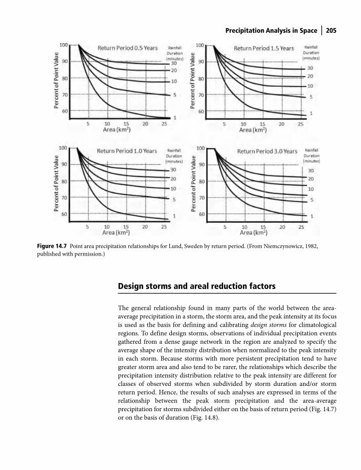
Precipitation Analysis in Space 205
Design storms and areal reduction factors
The general relationship found in many parts of the world between the area-
average precipitation in a storm, the storm area, and the peak intensity at its focus
is used as the basis for defining and calibrating design storms for climatological
regions. To define design storms, observations of individual precipitation events
gathered from a dense gauge network in the region are analyzed to specify the
average shape of the intensity distribution when normalized to the peak intensity
in each storm. Because storms with more persistent precipitation tend to have
greater storm area and also tend to be rarer, the relationships which describe the
precipitation intensity distribution relative to the peak intensity are different for
classes of observed storms when subdivided by storm duration and/or storm
return period. Hence, the results of such analyses are expressed in terms of the
relationship between the peak storm precipitation and the area-average
precipitation for storms subdivided either on the basis of return period (Fig. 14.7)
or on the basis of duration (Fig. 14.8).
Figure 14.7 Point area precipitation relationships for Lund, Sweden by return period. (From Niemczynowicz, 1982,
published with permission.)
Shuttleworth_c14.indd 205Shuttleworth_c14.indd 205 11/3/2011 7:02:45 PM11/3/2011 7:02:45 PM
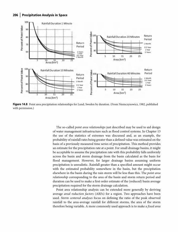
206 Precipitation Analysis in Space
The so-called point area relationships just described may be used to aid design
of water management infrastructure such as flood control systems. In Chapter 13
the use of the statistics of extremes was discussed and, as an example, the
probability of rainfall rates being greater than a defined value was estimated on the
basis of a previously measured time series of precipitation. This method provides
an estimate for the precipitation rate at a point. For small drainage basins, it might
be acceptable to assume the precipitation rate with this probability falls uniformly
across the basin and storm drainage from the basin calculated as the basis for
flood management. However, for larger drainage basins assuming uniform
precipitation is unrealistic. Rainfall greater than a specified amount might occur
with the estimated probability somewhere in the basin, but the precipitation
elsewhere in the basin during the rain storm will be less than this. The point area
relationship corresponding to the area of the basin and storm return period and
duration can be used to make a first order estimate of the (reduced) basin average
precipitation required for the storm drainage calculation.
Point area relationship analysis can be extended more generally by deriving
average areal reduction factors (ARFs) for a region. Two approaches have been
used. Storm centered analyses focus on defining the ratio of the peak observed
rainfall to the area-average rainfall for different storms, the area of the storm
therefore being variable. A more commonly used approach is to make a fixed area
Figure 14.8 Point area precipitation relationships for Lund, Sweden by duration. (From Niemczynowicz, 1982, published
with permission.)
Shuttleworth_c14.indd 206Shuttleworth_c14.indd 206 11/3/2011 7:02:46 PM11/3/2011 7:02:46 PM
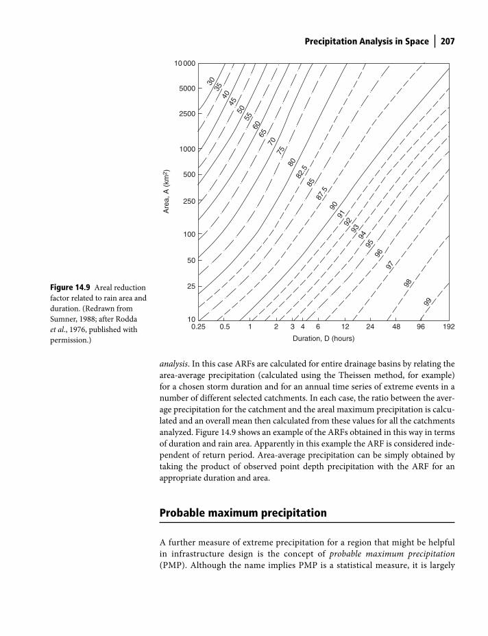
Precipitation Analysis in Space 207
analysis. In this case ARFs are calculated for entire drainage basins by relating the
area-average precipitation (calculated using the Theissen method, for example)
for a chosen storm duration and for an annual time series of extreme events in a
number of different selected catchments. In each case, the ratio between the aver-
age precipitation for the catchment and the areal maximum precipitation is calcu-
lated and an overall mean then calculated from these values for all the catchments
analyzed. Figure 14.9 shows an example of the ARFs obtained in this way in terms
of duration and rain area. Apparently in this example the ARF is considered inde-
pendent of return period. Area-average precipitation can be simply obtained by
taking the product of observed point depth precipitation with the ARF for an
appropriate duration and area.
Probable maximum precipitation
A further measure of extreme precipitation for a region that might be helpful
in infrastructure design is the concept of probable maximum precipitation
(PMP). Although the name implies PMP is a statistical measure, it is largely
0.25 0.5 1 2 3 4 6
Duration, D (hours)
12 24 48 96 192
99
98
97
96
9594
9392
9190
87.5
85
82.5
80
75
70
6560
5550
4540
3530
10 000
5000
2500
1000
500
250
100
50
25
10
Are
a, A
(km
2 )
Figure 14.9 Areal reduction
factor related to rain area and
duration. (Redrawn from
Sumner, 1988; after Rodda
et al., 1976, published with
permission.)
Shuttleworth_c14.indd 207Shuttleworth_c14.indd 207 11/3/2011 7:02:46 PM11/3/2011 7:02:46 PM
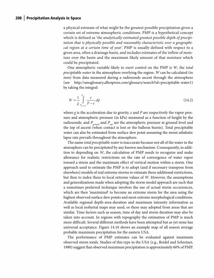
208 Precipitation Analysis in Space
a physical estimate of what might be the greatest possible precipitation given a
certain set of extreme atmospheric conditions. PMP is a hypothetical concept
which is defined as ‘the analytically estimated greatest possible depth of precipi-
tation that is physically possible and reasonably characteristic over a geographi-
cal region at a certain time of year’. PMP is usually defined with respect to a
given area, often a drainage basin, and includes estimates of the inflow of mois-
ture over the basin and the maximum likely amount of that moisture which
could be precipitated.
One atmospheric variable likely to exert control on the PMP is W, the total
precipitable water in the atmosphere overlying the region. W can be calculated (in
mm) from data measured during a radiosonde ascent through the atmosphere
(see http://amsglossary.allenpress.com/glossary/search?id=precipitable-water1)
by taking the integral:
1.
top
ground
P
P
eW dpg P e
=−∫ (14.2)
where g is the acceleration due to gravity, e and P are respectively the vapor pres-
sure and atmospheric pressure (in kPa) measured as a function of height by the
radiosonde, and Pground
and Ptop
are the atmospheric pressure at ground level and
the top of ascent (when contact is lost or the balloon bursts). Total precipitable
water can also be estimated from surface dew point assuming the moist adiabatic
lapse rate prevails throughout the atmosphere.
The name total precipitable water is inaccurate because not all of the water in the
atmosphere can be precipitated by any known mechanism. Consequently, in addi-
tion to depending on W, the calculation of PMP needs to recognize and make
allowance for realistic restrictions on the rate of convergence of water vapor
toward a storm and the maximum effect of vertical motion within a storm. One
approach used to estimate the PMP is to adopt (and if necessary transpose from
elsewhere) models of real extreme storms to estimate these additional restrictions,
but then to index these to local extreme values of W. However, the assumptions
and generalizations made when adopting the storm model approach are such that
a sometimes preferred technique involves the use of actual storm occurrences,
which are then ‘maximized’ to become an extreme storm for the area using the
highest observed surface dew points and most extreme morphological conditions.
Available regional depth-area-duration and maximum intensity information as
well as local isohyetal maps may used, or these may adopted from areas that are
similar. Time factors such as season, time of day and storm duration may also be
taken into account. In regions with topography the estimation of PMP is much
more difficult. Several different methods have been attempted but as yet none has
universal acceptance. Figure 14.10 shows an example map of all season average
probable maximum precipitation for the eastern USA.
The performance of PMP estimates can be evaluated against maximum
observed storm totals. Studies of this type in the USA (e.g., Reidel and Schreiner,
1980) suggest that observed maximum precipitation is approximately 60% of PMP.
Shuttleworth_c14.indd 208Shuttleworth_c14.indd 208 11/3/2011 7:02:46 PM11/3/2011 7:02:46 PM
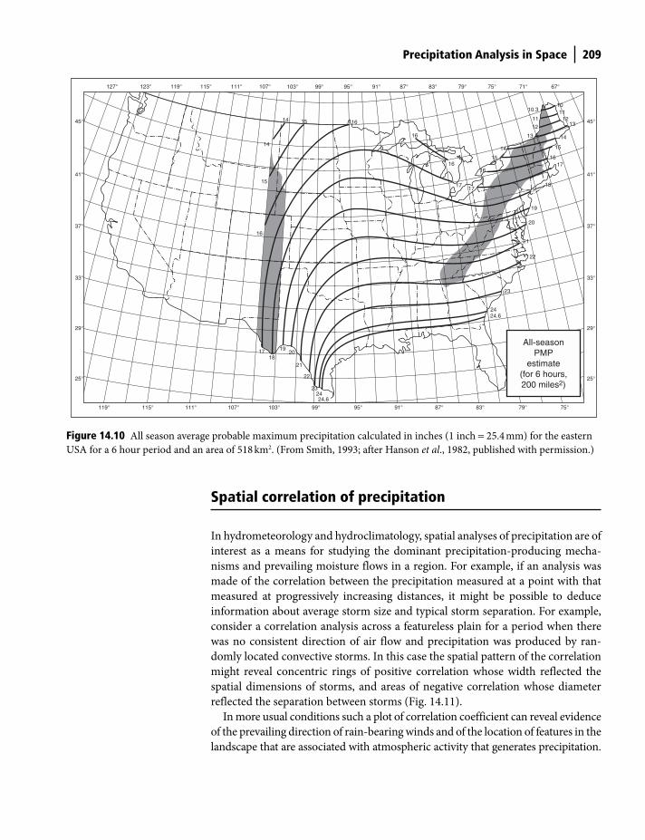
Precipitation Analysis in Space 209
Spatial correlation of precipitation
In hydrometeorology and hydroclimatology, spatial analyses of precipitation are of
interest as a means for studying the dominant precipitation-producing mecha-
nisms and prevailing moisture flows in a region. For example, if an analysis was
made of the correlation between the precipitation measured at a point with that
measured at progressively increasing distances, it might be possible to deduce
information about average storm size and typical storm separation. For example,
consider a correlation analysis across a featureless plain for a period when there
was no consistent direction of air flow and precipitation was produced by ran-
domly located convective storms. In this case the spatial pattern of the correlation
might reveal concentric rings of positive correlation whose width reflected the
spatial dimensions of storms, and areas of negative correlation whose diameter
reflected the separation between storms (Fig. 14.11).
In more usual conditions such a plot of correlation coefficient can reveal evidence
of the prevailing direction of rain-bearing winds and of the location of features in the
landscape that are associated with atmospheric activity that generates precipitation.
119°
25°
29°
33°
37°
41°
45°
25°
29°
33°
37°
41°
45°
127° 123° 119° 115° 111° 107° 103° 99° 95° 91° 87° 83° 79° 75° 71° 67°
115° 111° 107° 103° 99° 95° 91° 87° 83° 79° 75°
14
14
15
16
15 16
16
16
1717
15
16
14
13
12
11
10.31011
1213
14
15
16
18
19
20
21
22
23
2424.6
1718
1920
21
22
232424.6
All-seasonPMP
estimate(for 6 hours,200 miles2)
17
Figure 14.10 All season average probable maximum precipitation calculated in inches (1 inch = 25.4 mm) for the eastern
USA for a 6 hour period and an area of 518 km2. (From Smith, 1993; after Hanson et al., 1982, published with permission.)
Shuttleworth_c14.indd 209Shuttleworth_c14.indd 209 11/3/2011 7:02:47 PM11/3/2011 7:02:47 PM
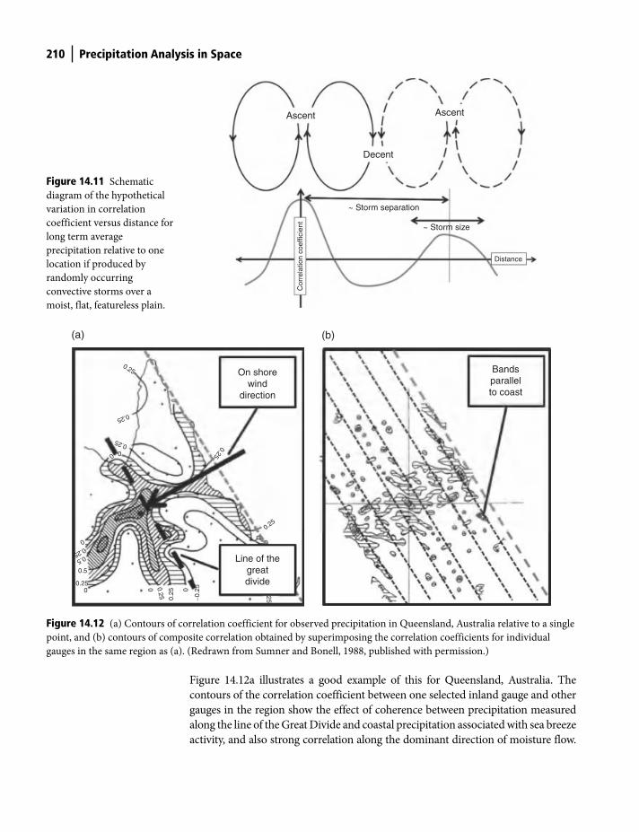
210 Precipitation Analysis in Space
Figure 14.12a illustrates a good example of this for Queensland, Australia. The
contours of the correlation coefficient between one selected inland gauge and other
gauges in the region show the effect of coherence between precipitation measured
along the line of the Great Divide and coastal precipitation associated with sea breeze
activity, and also strong correlation along the dominant direction of moisture flow.
Ascent Ascent
Decent
~ Storm separation
Distance
~ Storm size
Cor
rela
tion
coef
ficie
nt
Figure 14.11 Schematic
diagram of the hypothetical
variation in correlation
coefficient versus distance for
long term average
precipitation relative to one
location if produced by
randomly occurring
convective storms over a
moist, flat, featureless plain.
(a)
25On shore
winddirection
Line of thegreatdivide0.25
0.25
0.25
0.250.25
0.25
0.25
0
0
−0.2
5
0.5
0.5
0.25
0
0
0 0.25
(b)
Bandsparallelto coast
0
Figure 14.12 (a) Contours of correlation coefficient for observed precipitation in Queensland, Australia relative to a single
point, and (b) contours of composite correlation obtained by superimposing the correlation coefficients for individual
gauges in the same region as (a). (Redrawn from Sumner and Bonell, 1988, published with permission.)
Shuttleworth_c14.indd 210Shuttleworth_c14.indd 210 11/3/2011 7:02:48 PM11/3/2011 7:02:48 PM
Precipitation Analysis in Space 211
In some situations where the gauge density is high enough, it may also be possible to
create contour maps of composite correlation coefficient in which the correlation
fields for each gauge are superimposed. Figure 14.12b shows an example of a contour
map of composite correlation coefficient for this same area of Queensland showing
correlated bands of precipitation inland away from the coast separated by 40–45 km.
Important points in this chapter
● Mapping precipitation: drawing isohyets of precipitation involves esti-
mating the location of points with the required precipitation value between
pairs of gauge measurements then drawing smoothed isohyets through these
points.
● Area mean precipitation: is the value calculated as a weighted mean of
available precipitation observations, with weighting assigned in one of
several possible ways including using (a) the Isohyetal, (b) the Triangle, and
(c) the Theissen methods, although the Theissen method is often preferred
and all methods tend to produce similar results, especially if applied over a
long period.
● Spatial organization: storms tend to be organized in pseudo-elliptical or
linear groups, with individual storms elliptical in shape, more elongated
when larger, and with the rate of change in intensity increasing toward the
middle of the storm.
● Design storms: statistical analysis of observed storms results in the definition
of regional relationships between peak storm intensity and area-average
precipitation called areal reduction factors which are used in hydrological
design and which vary with storm duration and/or storm return period.
● Probable maximum precipitation (PMP): the hypothetical estimate for a
region of the greatest possible precipitation that might occur in extreme
atmospheric conditions over a specified area and period of time: it is variously
calculated but may be an overestimate relative to observed maximum
precipitation rates.
● Spatial correlation: spatial characteristics of the atmospheric mechanisms
involved in precipitation release in a region can be revealed by analysis of the
correlation between observations from a rain gauge network (see text).
References
Hanson, E.M., Schreiner, L.C. & Miller, J.F. (1982) Application of probable maximum pre-
cipitation estimates – United States east of the 105 meridian. Hydrometeorological Report
52, National Weather Service, NOAA, Washington, DC.
Niemczynowicz, J. (1982) Areal intensity-duration-frequency curves for short-term rainfall
events in Lund. Nordic Hydrology, 13, 193–204.
Shuttleworth_c14.indd 211Shuttleworth_c14.indd 211 11/3/2011 7:02:49 PM11/3/2011 7:02:49 PM

212 Precipitation Analysis in Space
Reidel, J. & Schreiner, L. (1980) Comparison of generalized estimates of probable maximum
precipitation with greatest observed rainfalls. NOAA Technical Report NWS 25, NOAA,
Washington, DC.
Rodda, J.C., Downey, R.A. & Law, F.M. (1976) Systematic Hydrology. Newnes-Butterworth,
London.
Smith, J.A. (1993) Precipitation. In: Maidment, D. (ed.) Handbook of Hydrology, pp. 3.1–4.1.
McGraw-Hill, New York.
Sumner, G.N. (1988) Precipitation Process and Analysis. John Wiley and Sons, Bath, UK.
Sumner, G.N. & Bonell, M. (1988) Variations in the spatial organization of daily rainfall
during the Queensland wet season. Theoretical and Applied Climatology, 39 (2), 59–74.
Shuttleworth_c14.indd 212Shuttleworth_c14.indd 212 11/3/2011 7:02:49 PM11/3/2011 7:02:49 PM

Introduction
The movement of momentum downward from the atmosphere into the Earth’s
surface and the transport of water vapor, heat, and minority gases between the
surface and the overlying atmosphere are primarily by the mechanism of turbulent
transport. Consequently, a basic understanding of the turbulence that occurs in
the atmospheric boundary layer is a necessary component of hydrometeorological
understanding. This chapter provides an introduction to the concept of atmos-
pheric turbulence and to the mathematical tools used when deriving equations
that describe it.
Signature and spectrum of atmospheric turbulence
If a fast response sensor of any weather variable is placed a few meters above the
ground in daytime conditions, the measurement it provides will reveal evidence of
apparently haphazard variability in the atmosphere. Figure 15.1 shows an example.
In this case the measurement recorded on the chart recorder trace shown is of
horizontal wind speed made with an anemometer capable of responding to
changes at a time scale of greater than 10 seconds. The measured wind speed is
recorded for about two and a half hours from 12:00 to 14:30 local time.
What does this chart recorder trace disclose? Careful inspection of Fig. 15.1
reveals the following.
a. There are clearly visible quasi-random fluctuations in the measured wind
speed, the pattern of which is not regular and not wave like.
b. The mean value of the measured wind speed is changing with time from around
6 m s−1 between 12:00 and12:30 to around 5 m s−1 between 14:00 and 14:30.
15 Mathematical and Conceptual Tools of Turbulence
Terrestrial Hydrometeorology, First Edition. W. James Shuttleworth.
© 2012 John Wiley & Sons, Ltd. Published 2012 by John Wiley & Sons, Ltd.
Shuttleworth_c15.indd 213Shuttleworth_c15.indd 213 11/3/2011 7:00:36 PM11/3/2011 7:00:36 PM

214 Mathematical and Conceptual Tools of Turbulence
c. The magnitude of the variability as characterized by variance of the trace
over 30 minutes decreases between 12:00 and 14:30.
d. There is arguably some evidence of structure in the variations, with small
peaks separated by about 1 minute superimposed on larger peaks at about
3–5 minutes, and some evidence of variations at about 8 to 10 minutes.
Because the measurement is of horizontal wind speed, the fact that there are
periods with faster and slower horizontal wind speed suggests the presence of
structures in the air flow that take about a minute to a few tens of minutes to
pass the fixed sensor. These, therefore, have a horizontal size on the order of
tens to thousands of meters (Fig. 15.2) and are sometimes referred to as
turbulent eddies.
Thus, observations made with a weather sensor mounted above the ground (in
this case an anemometer) show that there are haphazard variations in the meas-
13:000
5
10
Local time
Structure at 3–13 minsPeaks at about 1 min.
Mean 5 m s−1
Mean 6 m s−1
Win
d sp
eed
(m s
−1)
Change in variance
12:00 14:00
Figure 15.1 Trace of
horizontal wind speed
measured with an
anemometer. (Redrawn
from Stull, 1988,
published with
permission.)
1000’s m
Turbulent structures with differenthorizontal dimensions within a body
of air moving horizontally
10’s m
5 − 6 m s−1Figure 15.2 Schematic
diagram of turbulent eddies
circulating within an air
stream which is itself moving
at the mean wind speed.
Shuttleworth_c15.indd 214Shuttleworth_c15.indd 214 11/3/2011 7:00:37 PM11/3/2011 7:00:37 PM
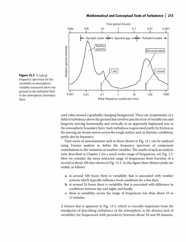
Mathematical and Conceptual Tools of Turbulence 215
ured value around a gradually changing background. These are symptomatic of a
field of turbulence above the ground that involves parcels of air of variable size and
longevity moving horizontally and vertically in an apparently haphazard way in
the atmospheric boundary layer. Such turbulence is generated partly by friction as
the moving air stream moves across the rough surface and, in daytime conditions,
partly also by buoyancy.
Time series of measurements such as those shown in Fig. 15.1 can be analysed
using Fourier analysis to define the frequency spectrum of component
contributions to the variations in weather variables. The results of such an analysis
were described in Chapter 1 for a much wider range of frequencies, see Fig. 1.3.
Here we consider the more restricted range of frequencies from fractions of a
second to about 100 days shown in Fig. 15.3. In this figure three distinct peaks are
visible, as follows:
a. at around 100 hours there is variability that is associated with weather
systems which typically influence local conditions for a few days;
b. at around 24 hours there is variability that is associated with difference in
conditions between day and night; and finally,
c. there is variability across the range of frequencies less than about 10 to
15 minutes.
A feature that is apparent in Fig. 15.3, which is crucially important from the
standpoint of describing turbulence in the atmosphere, is the distinct lack of
variability for frequencies with periodicity between about 30 and 90 minutes.
0.001
0.001
0.01
0.01
0.1
0.1
Eddy frequency (cycles per hour)
Time period (hours)
Rel
ativ
e sp
ectr
al in
tens
ity
10
10
100
100
1000
1000
1 day
Synoptic scale Turbulent scalesSpectral gap
Weathersystems
1 minute
Microscale eddies
1
1
Figure 15.3 A typical
frequency spectrum for the
variability in atmospheric
variables measured above the
ground in the turbulent field
in the atmospheric boundary
layer.
Shuttleworth_c15.indd 215Shuttleworth_c15.indd 215 11/3/2011 7:00:38 PM11/3/2011 7:00:38 PM
216 Mathematical and Conceptual Tools of Turbulence
This portion of the spectrum is called the spectra gap in variability and its
presence provides an opportunity to divide the representation of atmospheric
variability into two halves.
To the left of the spectral gap, variations are primarily associated with synoptic
scale features and with the more gradual change that occurs through the daily
cycle, such as the change in the mean value of wind speed between 12:00 and 14:00
already noticed in Fig. 15.1. To the right of the spectral gap, variations correspond
to the haphazard variability at higher frequency that are apparent in Fig. 15.1 and
are associated with turbulence. They reflect the movement of the parcels of air that
are continuously being created and destroyed in the turbulent field which, as they
move, provide the primary mechanism by means of which water vapor, heat,
momentum and chemical constituents are transported between the surface and
the atmosphere. Some important characteristics of turbulence to bear in mind in
what follows are:
● it is irregular and appears random, or at least pseudo-random, and because
of this a deterministic description of turbulence at all spatial scales is not
feasible;
● it is diffusive, and in most situations where turbulence occurs, the turbulent
transfer of energy, water vapor, momentum and atmospheric entities is much
more effective than transfer by molecular diffusion;
● it is three-dimensional, and entities such as plumes and vortexes can play a
significant role; and finally,
● it is continually being created and destroyed.
Mean and fluctuating components
Separating variations in atmospheric entities into low-frequency and high-
frequency variations is used as the basis for representing the turbulent atmos-
phere mathematically. Variations to the left of the spectral gap are described by
equations which are firmly based on physical principles such momentum, mass
and energy conservation, and which explicitly represent, or ‘resolve’, changes in
the ‘mean flow’ of atmospheric entities. Describing the haphazard turbulent vari-
ations that occur at higher frequencies that are to the right of the spectral gap in
Fig. 15.3 is less tractable. The most common approach is to represent their net
effect in the form of less well-grounded empirical equations, which are often
called ‘ parameterizations’. In later chapters it is shown that such parameterizations
are sometimes written in the form of empirical functions of the mean values of
atmospheric entities, these functions having been derived and calibrated by field
studies.
The first step toward writing a mathematical description of atmospheric changes
and movement is to re-write the value of each of the several atmospheric variables
in a form that explicitly recognizes that the variable has poorly described turbulent
Shuttleworth_c15.indd 216Shuttleworth_c15.indd 216 11/3/2011 7:00:39 PM11/3/2011 7:00:39 PM
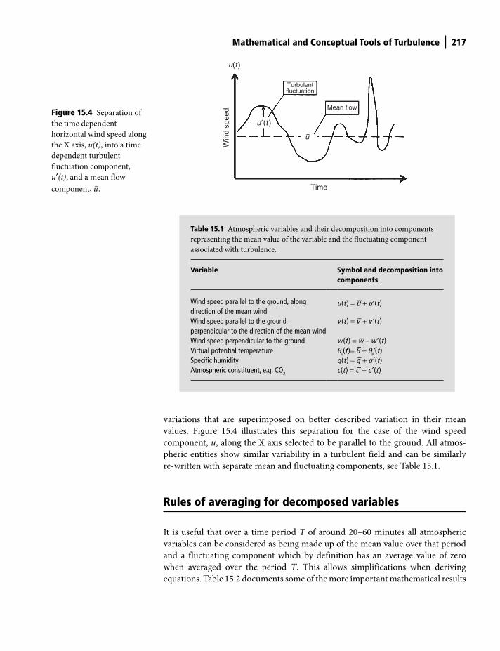
Mathematical and Conceptual Tools of Turbulence 217
variations that are superimposed on better described variation in their mean
values. Figure 15.4 illustrates this separation for the case of the wind speed
component, u, along the X axis selected to be parallel to the ground. All atmos-
pheric entities show similar variability in a turbulent field and can be similarly
re-written with separate mean and fluctuating components, see Table 15.1.
Rules of averaging for decomposed variables
It is useful that over a time period T of around 20–60 minutes all atmospheric
variables can be considered as being made up of the mean value over that period
and a fluctuating component which by definition has an average value of zero
when averaged over the period T. This allows simplifications when deriving
equations. Table 15.2 documents some of the more important mathematical results
Turbulentfluctuation
Mean flow
Time
u�(t )
u(t )
Win
d sp
eed
u
Figure 15.4 Separation of
the time dependent
horizontal wind speed along
the X axis, u(t), into a time
dependent turbulent
fluctuation component,
u′(t), and a mean flow
component, u–.
Table 15.1 Atmospheric variables and their decomposition into components
representing the mean value of the variable and the fluctuating component
associated with turbulence.
Variable Symbol and decomposition into components
Wind speed parallel to the ground, along direction of the mean wind
u(t ) = u– + u ′(t )
Wind speed parallel to the ground, perpendicular to the direction of the mean wind
v (t ) = v– + v ′(t )
Wind speed perpendicular to the ground w (t ) = w– + w ′(t )Virtual potential temperature qv(t )= q– + qv′(t )Specific humidity q(t ) = q– + q ′(t )Atmospheric constituent, e.g. CO2 c(t ) = c– + c ′(t )
Shuttleworth_c15.indd 217Shuttleworth_c15.indd 217 11/3/2011 7:00:39 PM11/3/2011 7:00:39 PM

218 Mathematical and Conceptual Tools of Turbulence
Table 15.2 Averaging rules for time-dependent variables A and B
re-written in terms of their mean and fluctuating components and a time
independent constant C.
Number Averaging rule Number Averaging rule
A1 C_ = C A6 ⎛ ⎞ =⎜ ⎟⎝ ⎠
dA d Adt dt
A2 ( )A B A B+ = + A7 A At t
∂ ∂⎛ ⎞ =⎜ ⎟⎝ ⎠∂ ∂
A3 =( )CA C A A8 ∂ ′ ∂ ′⎛ ⎞ =⎜ ⎟⎝ ⎠∂ ∂a at t
A4 ( )A A= and ( )B B= A9 ∂ ′ ∂ ′⎛ ⎞ =⎜ ⎟⎝ ⎠∂ ∂a a
A At t
A5 =( ) AB A B A10 ⎛ ⎞∂ ′ ∂ ′=⎜ ⎟∂ ∂⎝ ⎠
2 2( ) ( )a at t
that follow when two time dependent variables, A and B, are decomposed into
mean and fluctuating components and the mean value of their fluctuating
components is zero. In Table 15.2, A and B are as follows:
= + ′A A a (15.1)
and
= + ′B B b (15.2)
while C is a fixed constant that does not vary over the averaging period used to
define the mean and fluctuating components of A and B. In this table the presence
of an overbar over a variable implies that an average of that variable is taken over
the time period T.
One important (though obvious) result that immediately follows from these
rules is that because:
= + ′ = + ′ = + ′( ) ( ) ( )A A a A a A a (15.3)
it follows that:
′ = 0a (15.4)
Shuttleworth_c15.indd 218Shuttleworth_c15.indd 218 11/3/2011 7:00:39 PM11/3/2011 7:00:39 PM
Mathematical and Conceptual Tools of Turbulence 219
From Equation (15.4), it also follows that:
′ = ′ =( . ) 0B a B a (15.5)
and, by analogy, that:
′ = ′ =( . ) 0A b Ab (15.6)
Equations (15.5) and (15.6) can be used to demonstrate an important result. If one
takes the time-average of the cross product of two atmospheric variables, thus:
= + ′ + ′ = + ′ + ′ + ′ ′( ) ( )( ) ( )AB A a B b A B a B A b a b (15.7)
and then substitutes Equations (15.5) and (15.6) it follows that:
= + ′ ′( ) AB A B a b (15.8)
Thus, the time-average of the cross product of two atmospheric variables is equal
to the sum of two terms, the product of their mean values plus the time-average of
the instantaneous product of their fluctuating components over the period T. This
result is known as Reynolds averaging and it provides the basis for defining and
calculating measures of the strength of atmospheric turbulence and turbulent
fluxes, as described below. It is important to recognize that although Equations
(15.5) and (15.6) show the time-average of the product of a mean value with a
turbulent fluctuation is zero, in general, the time-average of the product of two or
more turbulent fluctuations cannot be assumed to be zero, thus ′ ′ ≠ 0a a , ′ ′ ≠ 0a b ,
′( ′) ≠2 0a b , ′ ′ ≠2 2( ) ( ) 0a b , etc.
Variance and standard deviation
The variance of an atmospheric variable, A, which has been re-written in terms of
mean and fluctuating parts, is formally defined by:
σ = + ′ − 22( ) (( ) )A A a A (15.9)
Multiplying out this equation and (for the purpose of illustrating their application)
applying the rules of averaging as used when deriving Equation (15.8), it follows
that:
σ = + ′ + ′ − + ′ +
= + ′ + ′ − − ′ +
2
2
( ) ( )( ) 2 ( )
2 ( ) 2 2
A A a A a A A a A A
A A A a a A A Aa A A (15.10)
Shuttleworth_c15.indd 219Shuttleworth_c15.indd 219 11/3/2011 7:00:52 PM11/3/2011 7:00:52 PM
220 Mathematical and Conceptual Tools of Turbulence
hence:
σ = ′2 2( ) ( )A a (15.11)
but note that in this case Equation (15.11) also follows directly from Equation
(15.9). From Equation (15.11), the standard deviation of A is given by:
σ = ′ 2( )A a (15.12)
Measures of the strength of turbulence
One measure of the strength of atmospheric turbulence is sm
, the square root of
the sum of the variances of the three orthogonal components of wind speed, u
parallel to the mean horizontal wind, v perpendicular to the mean horizontal
wind, and w in the vertical direction. sm
is calculated from:
σ = ′ + ′ + ′2 2 2( ) ( ) ( )m u v w (15.13)
Recall how the strength of the turbulence was judged to vary with time in Fig. 15.1.
Other measures of strength of turbulence can also be defined, including the turbu-
lent intensity, I, which is defined by normalizing sm
by the magnitude of the mean
wind vector, Um
, at the point where sm
was measured. Because Um
is given by:
= + +2 2 2( ) ( ) ( )mU u v w (15.14)
the turbulent intensity is given by:
′ + ′ + ′=+ +
2 2 2
2 2 2
( ) ( ) ( )
( ) ( ) ( )
u v wIu v w
(15.15)
Mean and turbulent kinetic energy
The kinetic energy, EK, of a body of mass M moving with a speed V is given by:
21
2kE MV= (15.16)
When defining the kinetic energy of air in the atmosphere it is usual to normalize
by the density of air to give the turbulent energy per unit mass and to separate the
kinetic energy associated with the mean air flow and the turbulent fluctuations
Shuttleworth_c15.indd 220Shuttleworth_c15.indd 220 11/3/2011 7:01:02 PM11/3/2011 7:01:02 PM
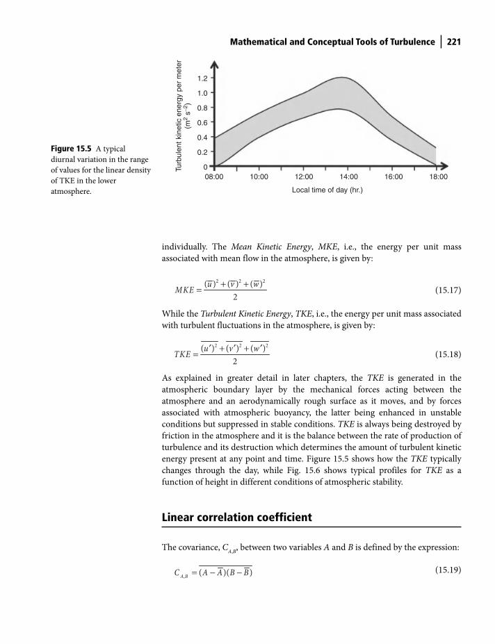
Mathematical and Conceptual Tools of Turbulence 221
individually. The Mean Kinetic Energy, MKE, i.e., the energy per unit mass
associated with mean flow in the atmosphere, is given by:
+ +=2 2 2( ) ( ) ( )
2
u v wMKE (15.17)
While the Turbulent Kinetic Energy, TKE, i.e., the energy per unit mass associated
with turbulent fluctuations in the atmosphere, is given by:
′ + ′ + ′=2 2 2( ) ( ) ( )
2
u v wTKE (15.18)
As explained in greater detail in later chapters, the TKE is generated in the
atmospheric boundary layer by the mechanical forces acting between the
atmosphere and an aerodynamically rough surface as it moves, and by forces
associated with atmospheric buoyancy, the latter being enhanced in unstable
conditions but suppressed in stable conditions. TKE is always being destroyed by
friction in the atmosphere and it is the balance between the rate of production of
turbulence and its destruction which determines the amount of turbulent kinetic
energy present at any point and time. Figure 15.5 shows how the TKE typically
changes through the day, while Fig. 15.6 shows typical profiles for TKE as a
function of height in different conditions of atmospheric stability.
Linear correlation coefficient
The covariance, CA,B
, between two variables A and B is defined by the expression:
= − −,
( )( )A BC A A B B (15.19)
08:000
0.2
0.4
0.6
0.8
1.0
1.2
10:00 12:00 14:00
Local time of day (hr.)
Turb
ulen
t kin
etic
ene
rgy
per
met
er(m
2 s−2
)16:00 18:00
Figure 15.5 A typical
diurnal variation in the range
of values for the linear density
of TKE in the lower
atmosphere.
Shuttleworth_c15.indd 221Shuttleworth_c15.indd 221 11/3/2011 7:01:07 PM11/3/2011 7:01:07 PM
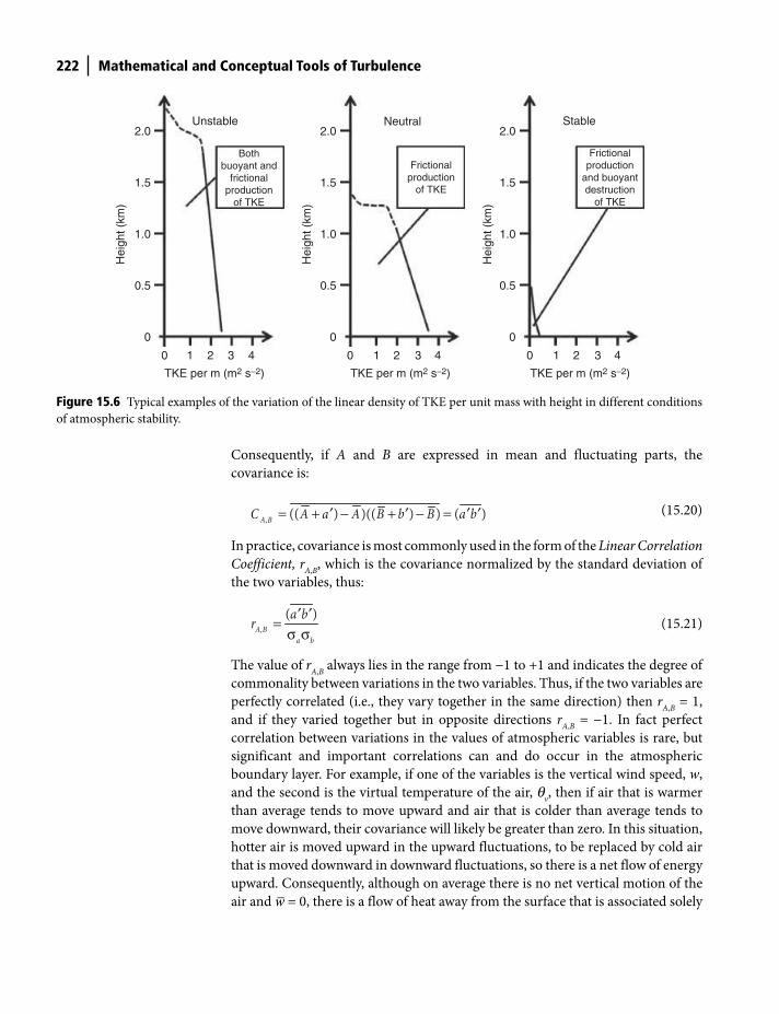
222 Mathematical and Conceptual Tools of Turbulence
Consequently, if A and B are expressed in mean and fluctuating parts, the
covariance is:
= + ′ − + ′ − = ′ ′,
(( ) )(( ) ) ( )A BC A a A B b B a b (15.20)
In practice, covariance is most commonly used in the form of the Linear Correlation
Coefficient, rA,B
, which is the covariance normalized by the standard deviation of
the two variables, thus:
′ ′=σ σ,
( )A B
a b
a br (15.21)
The value of rA,B
always lies in the range from −1 to +1 and indicates the degree of
commonality between variations in the two variables. Thus, if the two variables are
perfectly correlated (i.e., they vary together in the same direction) then rA,B
= 1,
and if they varied together but in opposite directions rA,B
= −1. In fact perfect
correlation between variations in the values of atmospheric variables is rare, but
significant and important correlations can and do occur in the atmospheric
boundary layer. For example, if one of the variables is the vertical wind speed, w,
and the second is the virtual temperature of the air, qv, then if air that is warmer
than average tends to move upward and air that is colder than average tends to
move downward, their covariance will likely be greater than zero. In this situation,
hotter air is moved upward in the upward fluctuations, to be replaced by cold air
that is moved downward in downward fluctuations, so there is a net flow of energy
upward. Consequently, although on average there is no net vertical motion of the
air and w_
= 0, there is a flow of heat away from the surface that is associated solely
0
0
0.5
1.0
1.5
2.0
1 2 3
TKE per m (m2 s−2)
Bothbuoyant and
frictionalproduction
of TKE
UnstableH
eigh
t (km
)
4 0
0
0.5
1.0
1.5
2.0
1 2 3
TKE per m (m2 s−2)
Stable
Hei
ght (
km)
4
Frictionalproduction
and buoyantdestruction
of TKE
0
0
0.5
1.0
1.5
2.0
1 2 3
TKE per m (m2 s−2)
Frictionalproduction
of TKE
Neutral
Hei
ght (
km)
4
Figure 15.6 Typical examples of the variation of the linear density of TKE per unit mass with height in different conditions
of atmospheric stability.
Shuttleworth_c15.indd 222Shuttleworth_c15.indd 222 11/3/2011 7:01:11 PM11/3/2011 7:01:11 PM
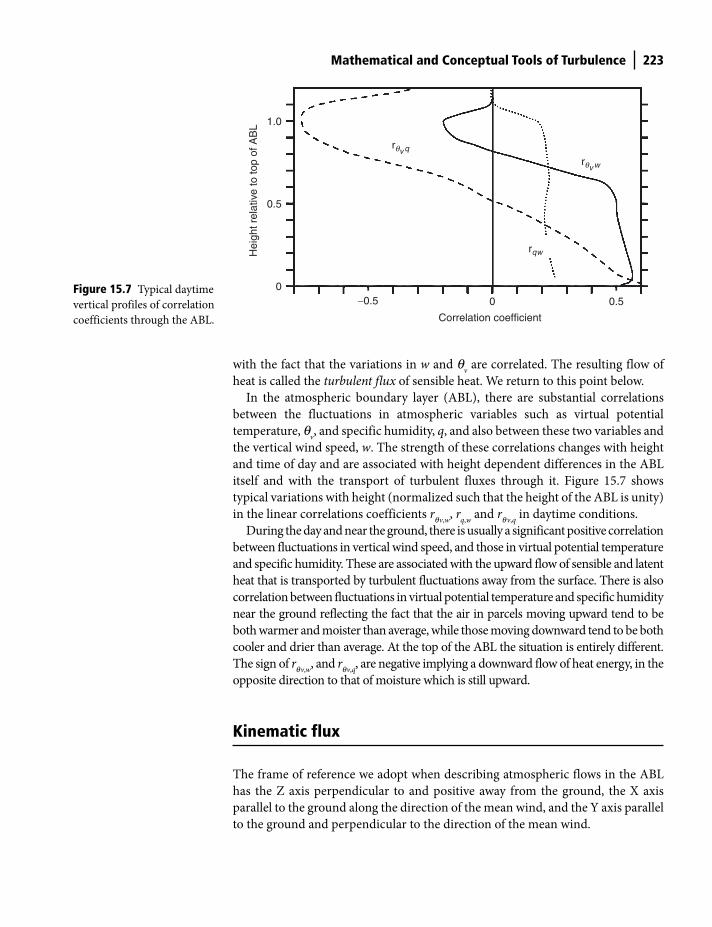
Mathematical and Conceptual Tools of Turbulence 223
with the fact that the variations in w and qv are correlated. The resulting flow of
heat is called the turbulent flux of sensible heat. We return to this point below.
In the atmospheric boundary layer (ABL), there are substantial correlations
between the fluctuations in atmospheric variables such as virtual potential
temperature, qv, and specific humidity, q, and also between these two variables and
the vertical wind speed, w. The strength of these correlations changes with height
and time of day and are associated with height dependent differences in the ABL
itself and with the transport of turbulent fluxes through it. Figure 15.7 shows
typical variations with height (normalized such that the height of the ABL is unity)
in the linear correlations coefficients rqv,w, r
q,w and rqv,q
in daytime conditions.
During the day and near the ground, there is usually a significant positive correlation
between fluctuations in vertical wind speed, and those in virtual potential temperature
and specific humidity. These are associated with the upward flow of sensible and latent
heat that is transported by turbulent fluctuations away from the surface. There is also
correlation between fluctuations in virtual potential temperature and specific humidity
near the ground reflecting the fact that the air in parcels moving upward tend to be
both warmer and moister than average, while those moving downward tend to be both
cooler and drier than average. At the top of the ABL the situation is entirely different.
The sign of rqv,w, and rqv,q
, are negative implying a downward flow of heat energy, in the
opposite direction to that of moisture which is still upward.
Kinematic flux
The frame of reference we adopt when describing atmospheric flows in the ABL
has the Z axis perpendicular to and positive away from the ground, the X axis
parallel to the ground along the direction of the mean wind, and the Y axis parallel
to the ground and perpendicular to the direction of the mean wind.
−0.5
rqv q
rqv w
rq w
0.5
1.0
0
Correlation coefficient
Hei
ght r
elat
ive
to to
p of
AB
L
00.5
Figure 15.7 Typical daytime
vertical profiles of correlation
coefficients through the ABL.
Shuttleworth_c15.indd 223Shuttleworth_c15.indd 223 11/3/2011 7:01:13 PM11/3/2011 7:01:13 PM

224 Mathematical and Conceptual Tools of Turbulence
The flux of any entity is the average value of the product of the volume density
relevant to that entity with the velocity of the air in the required direction. For
example, the flux of water vapor in the X direction over a specified period is the
time-average of:
(mass of water vapor per unit volume) × (velocity of air in X direction)
This water vapor flux, ρ( )aq u , therefore has units of (kg m−3) × (kgwater
kg−1) ×
(m s−1), or kgwater
m−2 s−1. Similarly, the sensible heat flux in the Y direction is the
time-average of:
(heat content per unit volume of air) × (velocity in Y direction)
Consequently, this sensible heat flux, ( )a p vc vr q , has units of (kg m−3) × (J kg−1 K−1) ×
(K) × (m s−1), or J m−2 s−1. And the flux of the Y component of momentum (recall
momentum is a vector) transferred in the Z direction is the time-average of:
(momentum flux in the Y direction per unit volume of air) × (velocity in Z direction)
Hence, this momentum flux, ( )au wr , has units of (kg m−3) × (m s−1) × (m s−1), or
kg m−1 s−2.
However, such entities as ‘heat content per unit volume of air’ and ‘momentum in
the Y direction per unit volume of air’ are either rarely measured or they are
unmeasureable. Rather, it is the equivalent entities, namely ‘virtual potential tem-
perature’ or ‘velocity in the Y direction’ that are measured instead. A product of a
measurable atmospheric entity with a velocity component can thus be related to a
true flux with appropriate physical dimensions, but it has the advantage that it
appears naturally when cross products between atmospheric variables are defined.
Partly because of this, but also because (as shown later) doing so simplifies the
suite of equations that describe atmospheric flow and makes them more comparable
with each other, it is convenient to redefine the fluxes of mass, sensible heat,
momentum and moisture and minority constituents. This is done by dividing by the
density of moist air or, in the particular case of sensible heat, by the product of the
density of moist air with the specific heat of air. It is viable to do this because changes
in the density of air are typically 10% or less through the depth of the atmospheric
boundary layer. The equivalent flux so defined is called the kinematic flux.
Thus, each true flux expressed in appropriate physical units can be associated
with a kinematic flux in different units that is the cross product of a measurable
atmospheric variable with a measureable velocity component. Table 15.3 lists the
true fluxes and their units, the measurable atmospheric entities equivalent to each
flux, the relationship between each pair of actual and kinematic fluxes, and the
dimensions of the equivalent kinematic flux. The description of the theory of tur-
bulence that follows in later chapters is given using kinematic fluxes. However, it
is important to remember that each kinematic flux must ultimately be recast back
into a true flux in appropriate units, as for example when used in equations
describing surface energy exchange.
Shuttleworth_c15.indd 224Shuttleworth_c15.indd 224 11/3/2011 7:01:13 PM11/3/2011 7:01:13 PM
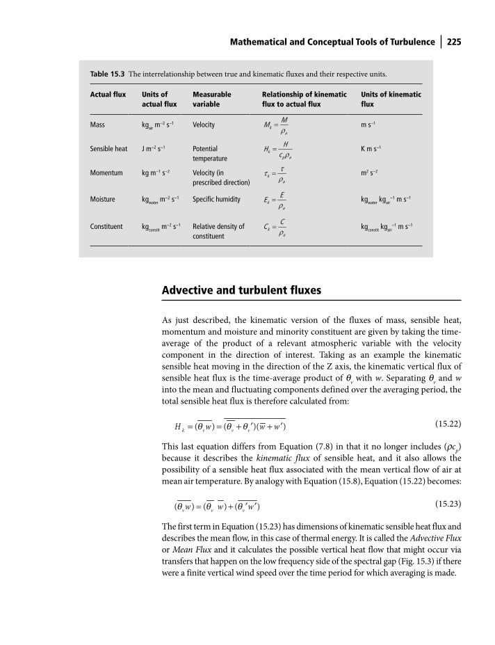
Mathematical and Conceptual Tools of Turbulence 225
Table 15.3 The interrelationship between true and kinematic fluxes and their respective units.
Actual flux Units of actual flux
Measurable variable
Relationship of kinematic flux to actual flux
Units of kinematic flux
Mass kgair m−2 s−1 Velocity =k
a
MM
ρm s−1
Sensible heat J m−2 s−1 Potential temperature
kp a
HH
c ρ= K m s−1
Momentum kg m−1 s−2 Velocity (in prescribed direction)
ka
ττρ
= m2 s−2
Moisture kgwater m−2 s−1 Specific humidity k
a
EE
ρ= kgwater kgair
−1 m s−1
Constituent kgconstit m−2 s−1 Relative density of
constituentk
a
CC
ρ= kgconstit kgair
−1 m s−1
Advective and turbulent fluxes
As just described, the kinematic version of the fluxes of mass, sensible heat,
momentum and moisture and minority constituent are given by taking the time-
average of the product of a relevant atmospheric variable with the velocity
component in the direction of interest. Taking as an example the kinematic
sensible heat moving in the direction of the Z axis, the kinematic vertical flux of
sensible heat flux is the time-average product of qv with w. Separating q
v and w
into the mean and fluctuating components defined over the averaging period, the
total sensible heat flux is therefore calculated from:
= = + ′ + ′( ) ( )( )k v v vH w w wq q q (15.22)
This last equation differs from Equation (7.8) in that it no longer includes (rcp)
because it describes the kinematic flux of sensible heat, and it also allows the
possibility of a sensible heat flux associated with the mean vertical flow of air at
mean air temperature. By analogy with Equation (15.8), Equation (15.22) becomes:
= + ′ ′( ) ( ) ( )v v vw w wq q q (15.23)
The first term in Equation (15.23) has dimensions of kinematic sensible heat flux and
describes the mean flow, in this case of thermal energy. It is called the Advective Flux
or Mean Flux and it calculates the possible vertical heat flow that might occur via
transfers that happen on the low frequency side of the spectral gap (Fig. 15.3) if there
were a finite vertical wind speed over the time period for which averaging is made.
Shuttleworth_c15.indd 225Shuttleworth_c15.indd 225 11/3/2011 7:01:16 PM11/3/2011 7:01:16 PM
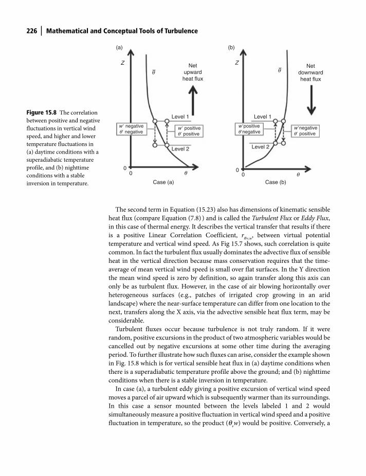
226 Mathematical and Conceptual Tools of Turbulence
The second term in Equation (15.23) also has dimensions of kinematic sensible
heat flux (compare Equation (7.8) ) and is called the Turbulent Flux or Eddy Flux,
in this case of thermal energy. It describes the vertical transfer that results if there
is a positive Linear Correlation Coefficient, rqv,w, between virtual potential
temperature and vertical wind speed. As Fig 15.7 shows, such correlation is quite
common. In fact the turbulent flux usually dominates the advective flux of sensible
heat in the vertical direction because mass conservation requires that the time-
average of mean vertical wind speed is small over flat surfaces. In the Y direction
the mean wind speed is zero by definition, so again transfer along this axis can
only be as turbulent flux. However, in the case of air blowing horizontally over
heterogeneous surfaces (e.g., patches of irrigated crop growing in an arid
landscape) where the near-surface temperature can differ from one location to the
next, transfers along the X axis, via the advective sensible heat flux term, may be
considerable.
Turbulent fluxes occur because turbulence is not truly random. If it were
random, positive excursions in the product of two atmospheric variables would be
cancelled out by negative excursions at some other time during the averaging
period. To further illustrate how such fluxes can arise, consider the example shown
in Fig. 15.8 which is for vertical sensible heat flux in (a) daytime conditions when
there is a superadiabatic temperature profile above the ground; and (b) nighttime
conditions when there is a stable inversion in temperature.
In case (a), a turbulent eddy giving a positive excursion of vertical wind speed
moves a parcel of air upward which is subsequently warmer than its surroundings.
In this case a sensor mounted between the levels labeled 1 and 2 would
simultaneously measure a positive fluctuation in vertical wind speed and a positive
fluctuation in temperature, so the product (qvw) would be positive. Conversely, a
0
Case (a)
w� positiveq� positive
w�positiveq�negative
w� negativeq� negative
w�negativeq� positive
Z Z
Level 2
Level 1
Level 2
Level 1
Netupwardheat flux
(a) (b)
Netdownwardheat flux
q 0Case (b)
q0 0
q q
Figure 15.8 The correlation
between positive and negative
fluctuations in vertical wind
speed, and higher and lower
temperature fluctuations in
(a) daytime conditions with a
superadiabatic temperature
profile, and (b) nighttime
conditions with a stable
inversion in temperature.
Shuttleworth_c15.indd 226Shuttleworth_c15.indd 226 11/3/2011 7:01:23 PM11/3/2011 7:01:23 PM
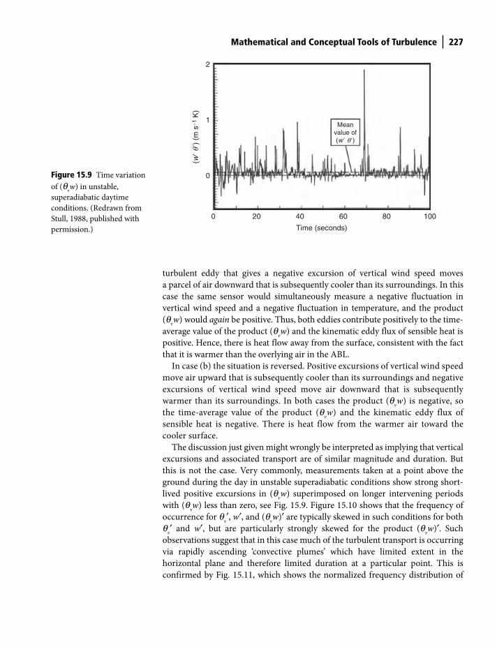
Mathematical and Conceptual Tools of Turbulence 227
turbulent eddy that gives a negative excursion of vertical wind speed moves
a parcel of air downward that is subsequently cooler than its surroundings. In this
case the same sensor would simultaneously measure a negative fluctuation in
vertical wind speed and a negative fluctuation in temperature, and the product
(qvw) would again be positive. Thus, both eddies contribute positively to the time-
average value of the product (qvw) and the kinematic eddy flux of sensible heat is
positive. Hence, there is heat flow away from the surface, consistent with the fact
that it is warmer than the overlying air in the ABL.
In case (b) the situation is reversed. Positive excursions of vertical wind speed
move air upward that is subsequently cooler than its surroundings and negative
excursions of vertical wind speed move air downward that is subsequently
warmer than its surroundings. In both cases the product (qvw) is negative, so
the time-average value of the product (qvw) and the kinematic eddy flux of
sensible heat is negative. There is heat flow from the warmer air toward the
cooler surface.
The discussion just given might wrongly be interpreted as implying that vertical
excursions and associated transport are of similar magnitude and duration. But
this is not the case. Very commonly, measurements taken at a point above the
ground during the day in unstable superadiabatic conditions show strong short-
lived positive excursions in (qvw) superimposed on longer intervening periods
with (qvw) less than zero, see Fig. 15.9. Figure 15.10 shows that the frequency of
occurrence for qv′, w′, and (q
vw)′ are typically skewed in such conditions for both
qv′ and w′, but are particularly strongly skewed for the product (q
vw)′. Such
observations suggest that in this case much of the turbulent transport is occurring
via rapidly ascending ‘convective plumes’ which have limited extent in the
horizontal plane and therefore limited duration at a particular point. This is
confirmed by Fig. 15.11, which shows the normalized frequency distribution of
0
0
1
2
20 40 60
Time (seconds)
Meanvalue of(w� q�)
(w�
q�)
(m s
−1 K
)
80 100
Figure 15.9 Time variation
of (qvw) in unstable,
superadiabatic daytime
conditions. (Redrawn from
Stull, 1988, published with
permission.)
Shuttleworth_c15.indd 227Shuttleworth_c15.indd 227 11/3/2011 7:01:23 PM11/3/2011 7:01:23 PM
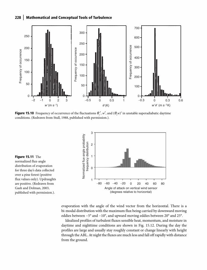
228 Mathematical and Conceptual Tools of Turbulence
−2 −1 00
50Fre
quen
cy o
f occ
urre
nce
100
150
200
250
w �(m s−1)
2 3 −0.5 00
50
Fre
quen
cy o
f occ
urre
nce
100
150
200
250
300
q�(K)
0.5 1 −0.3 00
100
Fre
quen
cy o
f occ
urre
nce
200
300
400
500
600
700
w�q� (m s−1K)
0.3 0.6
Figure 15.10 Frequency of occurrence of the fluctuations qv′, w′, and (q
vw)′ in unstable superadiabatic daytime
conditions. (Redrawn from Stull, 1988, published with permission.).
−80
0
1
2
1
3
−60 −40 −20 80604020
Angle of attack on vertical wind sensor(degrees relative to horizontal)
Nor
mal
ized
flux
-ang
le p
roba
bilit
yfr
eque
ncy
dist
ribut
ion
0
Figure 15.11 The
normalized flux-angle
distribution of evaporation
for three day’s data collected
over a pine forest (positive
flux values only). Updraughts
are positive. (Redrawn from
Gash and Dolman, 2003,
published with permission.).
evaporation with the angle of the wind vector from the horizontal. There is a
bi-modal distribution with the maximum flux being carried by downward moving
eddies between −5° and −10°, and upward moving eddies between 20° and 25°.
Idealized profiles of turbulent fluxes sensible heat, momentum, and moisture in
daytime and nighttime conditions are shown in Fig. 15.12. During the day the
profiles are large and usually stay roughly constant or change linearly with height
through the ABL. At night the fluxes are much less and fall off rapidly with distance
from the ground.
Shuttleworth_c15.indd 228Shuttleworth_c15.indd 228 11/3/2011 7:01:24 PM11/3/2011 7:01:24 PM
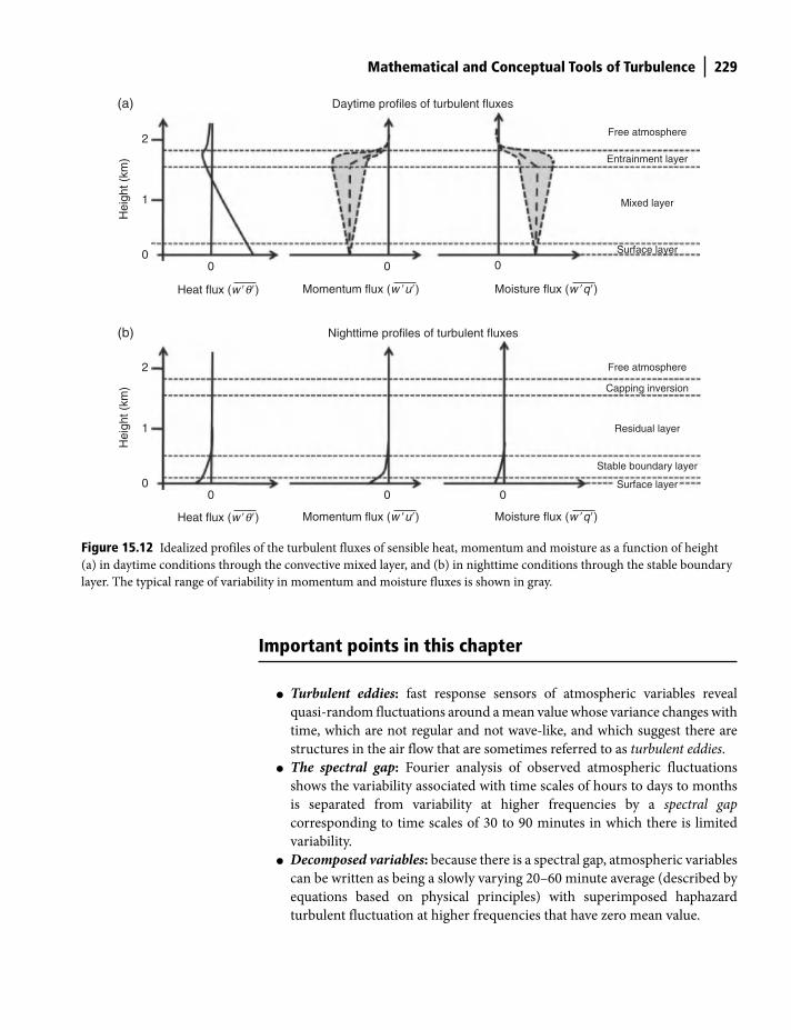
Mathematical and Conceptual Tools of Turbulence 229
Important points in this chapter
● Turbulent eddies: fast response sensors of atmospheric variables reveal
quasi-random fluctuations around a mean value whose variance changes with
time, which are not regular and not wave-like, and which suggest there are
structures in the air flow that are sometimes referred to as turbulent eddies.
● The spectral gap: Fourier analysis of observed atmospheric fluctuations
shows the variability associated with time scales of hours to days to months
is separated from variability at higher frequencies by a spectral gap
corresponding to time scales of 30 to 90 minutes in which there is limited
variability.
● Decomposed variables: because there is a spectral gap, atmospheric variables
can be written as being a slowly varying 20–60 minute average (described by
equations based on physical principles) with superimposed haphazard
turbulent fluctuation at higher frequencies that have zero mean value.
00 0 0
Free atmosphere
Surface layer
Capping inversion
Residual layer
Stable boundary layer
Nighttime profiles of turbulent fluxes
1
Hei
ght (
km)
2
(b)
Free atmosphere
Surface layer
Mixed layer
Entrainment layer
Daytime profiles of turbulent fluxes
Heat flux (w�q�)
00 0 0
1
Hei
ght (
km)
2
Momentum flux (w �u�) Moisture flux (w �q�)
Heat flux (w�q�) Momentum flux (w �u�) Moisture flux (w �q�)
(a)
Figure 15.12 Idealized profiles of the turbulent fluxes of sensible heat, momentum and moisture as a function of height
(a) in daytime conditions through the convective mixed layer, and (b) in nighttime conditions through the stable boundary
layer. The typical range of variability in momentum and moisture fluxes is shown in gray.
Shuttleworth_c15.indd 229Shuttleworth_c15.indd 229 11/3/2011 7:01:24 PM11/3/2011 7:01:24 PM
230 Mathematical and Conceptual Tools of Turbulence
● Averaging rules: simplifying rules apply when the time-average is taken of
decomposed atmospheric variables, decomposed variables multiplied by a
constant, and derivatives and combinations of decomposed variables
(Table 15.2).
● Reynolds averaging: the cross product of two atmospheric variables is equal
to the product of their mean values plus the time-average of the instantane-
ous product of their fluctuating components: the time-average of the product
of two or more turbulent fluctuations cannot be assumed to be zero.
● Mean and turbulent kinetic energy: Mean Kinetic Energy (MKE) and
Turbulent Kinetic Energy (TKE) per unit mass of air are given by the sum of
the squares of the mean wind speed components and sum of the squares of
the turbulent wind speed components, respectively: TKE is not conserved.
● Correlation of variables: in the ABL there are substantial height- and time-
dependent correlations between the fluctuations in atmospheric variables
(e.g., virtual potential temperature, specific humidity, and vertical wind speed)
that are associated with the transport of turbulent fluxes within the ABL.
● Kinematic fluxes: to simplify the development of equations describing
atmospheric flow described in later chapters it is convenient to work in terms
of kinematic fluxes (e.g., Hk, E
k,, t
k,, etc), these being the fluxes in natural
units (e.g., H, E, t, etc) divided by r or, in the case of sensible heat, by (rcp).
● Advective and turbulent flux: a kinematic flux is the time-average of the
product of an atmospheric variable with the velocity component in the
direction of interest. Reynolds averaging identifies kinematic flux as the sum
of an advective flux (the product of their mean values), and a turbulent flux
(the time-average of the instantaneous product of their fluctuating
components).
References
Gash, J.H.C. and Dolman, A.J. 2003. Sonic anemometer (co)sine response and flux meas-
urement: I. The potential for cosine error to affect flux measurements. Agricultural and
Forest Meteorology, 119, 195–207.
Stull, R.B. (1988) An Introduction to Boundary Layer Meteorology (Atmospheric Sciences
Library). Kluger Academic Publishers, Dordrecht, Netherlands.
Shuttleworth_c15.indd 230Shuttleworth_c15.indd 230 11/3/2011 7:01:25 PM11/3/2011 7:01:25 PM
Introduction
This chapter introduces the set of equations that are used to describe the
movement and evolution of the atmosphere and its constituents at any point in
time. Later these equations are developed to provide a description of mean
atmospheric flow and atmospheric turbulence by separating the variables used
into mean and fluctuating components and then applying the Reynolds averaging
described in the chapter 15.
One of the equations meteorologists use to describe the atmosphere is the
ideal gas law introduced in Chapter 1. Otherwise, the set of equations used are
simply the conservation laws for mass, momentum, energy and atmospheric
constituents, including moisture. However, to those unfamiliar with them, these
conservation equations may appear complex because they typically involve
many terms. The need to include several terms arises because the conservation
laws are being applied in a complex situation, i.e., in a moving fluid which has
viscosity, which is subject to a gravitational force and constrained to the surface of
a rotating Earth, and which has constituents some of which can undergo phase
changes.
Nonetheless, it is important to understand that the equations are fundamen-
tally just conservation laws, and the approach used to define them in this chapter
reflects this. In each case, the rate of change with time of the local concentration
of each conserved entity is first defined, recognizing that it is the rate of change
appropriate in a moving fluid that is required. Then the several physical processes
that can give rise to changes in local concentration of the conserved entity are
each separately identified and expressed algebraically. The required conservation
equation follows immediately by setting the rate of change in local concentration
equal to the sum of the terms that describe how it might be altered.
16 Equations of Atmospheric Flow in the ABL
Terrestrial Hydrometeorology, First Edition. W. James Shuttleworth.
© 2012 John Wiley & Sons, Ltd. Published 2012 by John Wiley & Sons, Ltd.
Shuttleworth_c16.indd 231Shuttleworth_c16.indd 231 11/3/2011 6:56:22 PM11/3/2011 6:56:22 PM

232 Equations of Atmospheric Flow in the ABL
Because the equations describing the movement and evolution of atmospheric
properties are complex, sometimes they can be written more efficiently using
shorthand representations, including using the ‘summation convention’ and
‘vector algebra’. Use of such representations has merit for the specialist because it
allows conciseness. However, their use requires first creating familiarity with
the efficient representation adopted, and to those who are not fluent in the
language of the selected representation this can inhibit ready understanding.
In this chapter, the primary goal is to convey understanding of how the basic
equations that describe the atmosphere arise. For this reason, use of such efficient
representations is largely avoided and clumsiness in representation is accepted
if this is more likely to improve comprehension. However, vector algebra equa-
tions are occasionally introduced when this is unlikely to confuse.
For reasons of conciseness, not all the equations sought are derived indepen-
dently and completely in this chapter. Often it is possible to derive an equation in
one dimension and its form in the other two dimensions follows by analogy. Also,
the need for some terms in one conservation equation can be easily recognized by
analogy with equivalent terms in another conservation equation.
Time rate of change in a fluid
Most readers will understand the distinction between the total derivative and
the partial derivative of a variable. However, for those less confident in this
branch of mathematics it is useful to review why the rate of change of an
atmospheric variable with time is written as the sum of more than one term. To
do this the rate of change of momentum in the direction of the mean wind
parallel to the ground is used as an example.
In this chapter the selected frame of reference is defined such that the Z axis
is perpendicular to and positive away from the ground, the X axis is parallel to
the ground pointing east along the line of latitude, and the Y axis is parallel to the
ground along the line of longitude. Consider the rate of change with time of u
(the velocity along the X axis) at a point where the velocity of the moving air
has three components, u, v, and w along the X, Y, and Z axes respectively. For
simplicity, first consider the case when the air is only moving along the X axis.
Figure 16.1 illustrates that, in this case, there are two reasons why there may be a
change in the value of u at a particular point.
First, there may be a change in the value u at the point due to some (as yet
undefined) local force acting at that point (Fig. 16.1). This will give rise to a
change in the velocity component along the X axis which is represented by the
partial derivative of u with respect to time. However, even if there were no local
force acting, the air is moving past the point and the velocity along the X axis
within the moving body of air may not be constant. Consequently, the velocity in
the moving air as it passes at one time may be different to that within the air as it
passes at a later time (Fig. 16.1). The rate of change in the value of u resulting solely
Shuttleworth_c16.indd 232Shuttleworth_c16.indd 232 11/3/2011 6:56:23 PM11/3/2011 6:56:23 PM
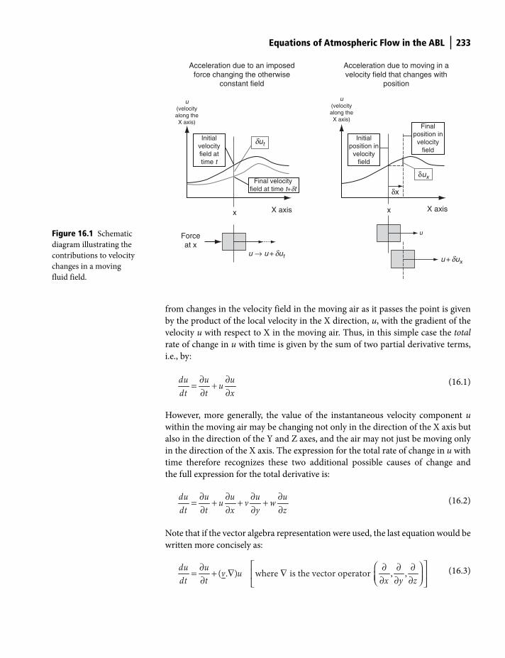
Equations of Atmospheric Flow in the ABL 233
from changes in the velocity field in the moving air as it passes the point is given
by the product of the local velocity in the X direction, u, with the gradient of the
velocity u with respect to X in the moving air. Thus, in this simple case the total
rate of change in u with time is given by the sum of two partial derivative terms,
i.e., by:
∂ ∂= +
∂ ∂du u u
udt t x
(16.1)
However, more generally, the value of the instantaneous velocity component u
within the moving air may be changing not only in the direction of the X axis but
also in the direction of the Y and Z axes, and the air may not just be moving only
in the direction of the X axis. The expression for the total rate of change in u with
time therefore recognizes these two additional possible causes of change and
the full expression for the total derivative is:
du u u u uu v w
dt t x y z
∂ ∂ ∂ ∂= + + +
∂ ∂ ∂ ∂
(16.2)
Note that if the vector algebra representation were used, the last equation would be
written more concisely as:
⎡ ⎤⎛ ⎞∂ ∂ ∂ ∂= + ∇ ∇⎢ ⎥⎜ ⎟∂ ∂ ∂ ∂⎝ ⎠⎣ ⎦( . ) where is the vector operator , ,
du uv u
dt t x y z
(16.3)
X axis
Final velocityfield at time t+dt
Initialvelocityfield attime t
Acceleration due to an imposedforce changing the otherwise
constant field
Acceleration due to moving in avelocity field that changes with
position
Initialposition in
velocityfield
Finalposition in
velocityfield
u(velocityalong theX axis)
u(velocityalong theX axis)
u
x X axisx
Forceat x
u → u + dut u + dux
δux
δx
dut
Figure 16.1 Schematic
diagram illustrating the
contributions to velocity
changes in a moving
fluid field.
Shuttleworth_c16.indd 233Shuttleworth_c16.indd 233 11/3/2011 6:56:23 PM11/3/2011 6:56:23 PM
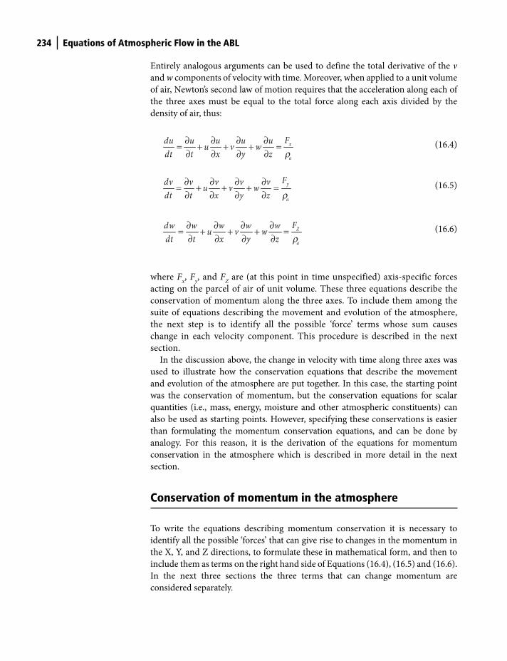
234 Equations of Atmospheric Flow in the ABL
Entirely analogous arguments can be used to define the total derivative of the v
and w components of velocity with time. Moreover, when applied to a unit volume
of air, Newton’s second law of motion requires that the acceleration along each of
the three axes must be equal to the total force along each axis divided by the
density of air, thus:
∂ ∂ ∂ ∂= + + + =
∂ ∂ ∂ ∂x
a
Fdu u u u uu v w
dt t x y z r
(16.4)
∂ ∂ ∂ ∂= + + + =
∂ ∂ ∂ ∂y
a
Fdv v v v vu v w
dt t x y z r
(16.5)
∂ ∂ ∂ ∂= + + + =
∂ ∂ ∂ ∂Z
a
Fdw w w w wu v w
dt t x y z r
(16.6)
where Fx, F
y, and F
Z are (at this point in time unspecified) axis-specific forces
acting on the parcel of air of unit volume. These three equations describe the
conservation of momentum along the three axes. To include them among the
suite of equations describing the movement and evolution of the atmosphere,
the next step is to identify all the possible ‘force’ terms whose sum causes
change in each velocity component. This procedure is described in the next
section.
In the discussion above, the change in velocity with time along three axes was
used to illustrate how the conservation equations that describe the movement
and evolution of the atmosphere are put together. In this case, the starting point
was the conservation of momentum, but the conservation equations for scalar
quantities (i.e., mass, energy, moisture and other atmospheric constituents) can
also be used as starting points. However, specifying these conservations is easier
than formulating the momentum conservation equations, and can be done by
analogy. For this reason, it is the derivation of the equations for momentum
conservation in the atmosphere which is described in more detail in the next
section.
Conservation of momentum in the atmosphere
To write the equations describing momentum conservation it is necessary to
identify all the possible ‘forces’ that can give rise to changes in the momentum in
the X, Y, and Z directions, to formulate these in mathematical form, and then to
include them as terms on the right hand side of Equations (16.4), (16.5) and (16.6).
In the next three sections the three terms that can change momentum are
considered separately.
Shuttleworth_c16.indd 234Shuttleworth_c16.indd 234 11/3/2011 6:56:26 PM11/3/2011 6:56:26 PM
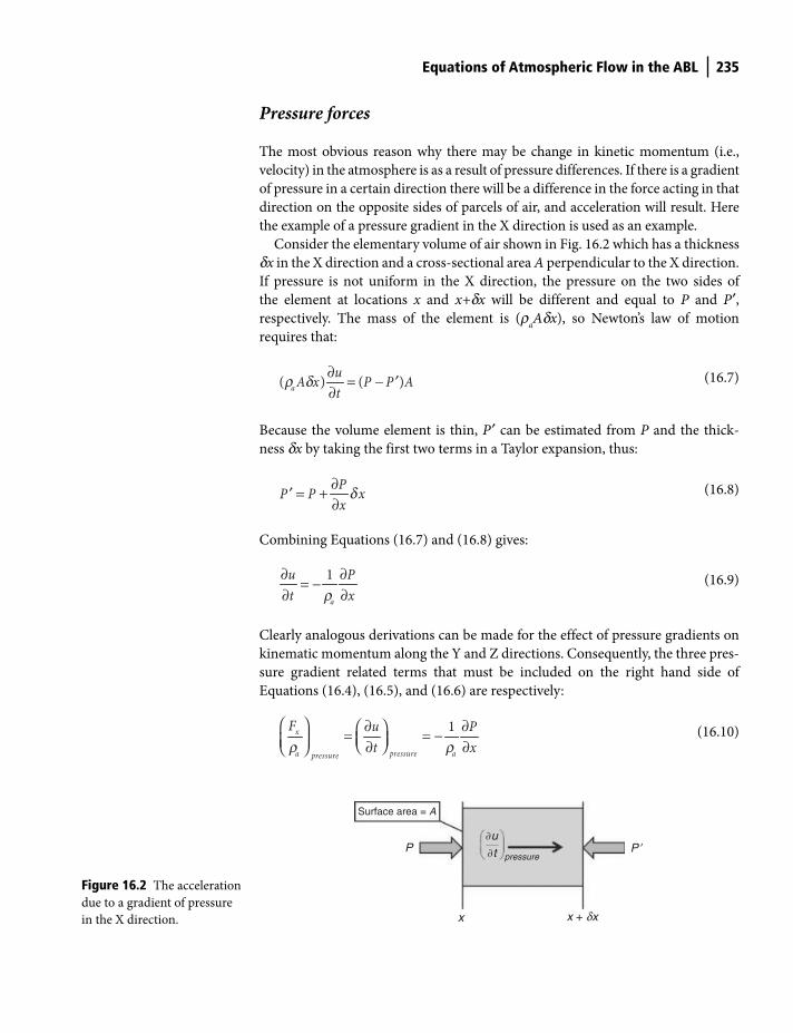
Equations of Atmospheric Flow in the ABL 235
Pressure forces
The most obvious reason why there may be change in kinetic momentum (i.e.,
velocity) in the atmosphere is as a result of pressure differences. If there is a gradient
of pressure in a certain direction there will be a difference in the force acting in that
direction on the opposite sides of parcels of air, and acceleration will result. Here
the example of a pressure gradient in the X direction is used as an example.
Consider the elementary volume of air shown in Fig. 16.2 which has a thickness
dx in the X direction and a cross-sectional area A perpendicular to the X direction.
If pressure is not uniform in the X direction, the pressure on the two sides of
the element at locations x and x+dx will be different and equal to P and P′, respectively. The mass of the element is (r
aAdx), so Newton’s law of motion
requires that:
∂ = − ′∂
( ) ( )a
uA x P P A
tr d
(16.7)
Because the volume element is thin, P′ can be estimated from P and the thick-
ness dx by taking the first two terms in a Taylor expansion, thus:
∂′ = +∂P
P P xx
d
(16.8)
Combining Equations (16.7) and (16.8) gives:
∂ ∂= −
∂ ∂1
a
u P
t xr
(16.9)
Clearly analogous derivations can be made for the effect of pressure gradients on
kinematic momentum along the Y and Z directions. Consequently, the three pres-
sure gradient related terms that must be included on the right hand side of
Equations (16.4), (16.5), and (16.6) are respectively:
⎛ ⎞ ∂ ∂⎛ ⎞= = −⎜ ⎟⎜ ⎟ ⎝ ⎠∂ ∂⎝ ⎠1x
a pressure apressure
F u P
t xr r
(16.10)
x
Surface area = A
pressure
�uP P �
x + dx
�t
Figure 16.2 The acceleration
due to a gradient of pressure
in the X direction.
Shuttleworth_c16.indd 235Shuttleworth_c16.indd 235 11/3/2011 6:56:29 PM11/3/2011 6:56:29 PM
236 Equations of Atmospheric Flow in the ABL
⎛ ⎞ ∂ ∂⎛ ⎞= = −⎜ ⎟⎜ ⎟ ⎝ ⎠∂ ∂⎝ ⎠1y
a pressure apressure
F v P
t yr r
(16.11)
⎛ ⎞ ∂ ∂⎛ ⎞= = −⎜ ⎟⎜ ⎟ ⎝ ⎠∂ ∂⎝ ⎠1z
a pressure apressure
F w P
t zr r
(16.12)
Were we to use vector algebra formulation for Equations (16.10), (16.11), and
(16.12) these three equations would be written more concisely as a single vector
equation, thus:
⎛ ⎞ ∂⎛ ⎞= = − ∇⎜ ⎟⎜ ⎟ ⎝ ⎠∂⎝ ⎠ pressurepressure
1
a a
F vP
tr r
(16.13)
Viscous flow in fluids
A second way that the velocity component of a small parcel of air might change at
a particular point is if, as a result of the molecular movements in the air, there is a
net transfer to that point of momentum in the direction of interest. In other words
if, for example, there is more momentum in the X direction diffusing into the par-
cel by molecular diffusion than is diffusing out of the parcel, the local velocity of
the parcel in the X direction will increase. We therefore expect that one of the
‘force’ terms needed on the right hand side of Equations (16.4), (16.5), and (16.6)
will quantify the effect of any imbalance in the amount of momentum in each
direction entering and leaving at the point where the equations are applied. The
next step is, therefore, to consider the equations which describe the molecular dif-
fusion of momentum in air and, from these, to define the term that calculates the
local imbalance for each axis.
The equation describing molecular transfer of momentum in fluids was written
by Newton many centuries ago. It is framed in terms of the viscosity of the fluid,
which is a basic molecular property of the fluid (in the present case, air) that is a
measure of the fluid’s internal resistance to deformation. In other words, it defines
the ease with which (hypothetically) parallel layers of fluid can slip past each other.
Figure 16.3 illustrates a two-dimensional example in which a fluid is undergoing
smooth, streamlined, laminar (i.e., not turbulent) flow in the X direction between
two very large parallel plates separated by a distance h.
Consider the variation in velocity in the Z direction which is perpendicular to
the two plates. In this case, the velocity u in the X direction varies uniformly from
zero at the lower plate to Uh at the upper plate and:
hUu
z h
∂=
∂ (16.14)
Shuttleworth_c16.indd 236Shuttleworth_c16.indd 236 11/3/2011 6:56:33 PM11/3/2011 6:56:33 PM
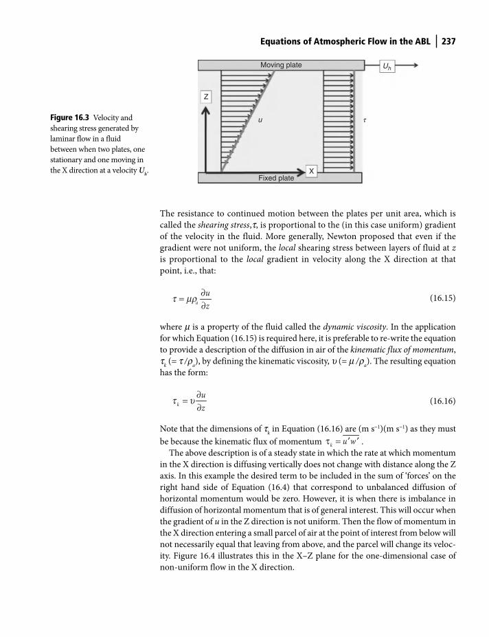
Equations of Atmospheric Flow in the ABL 237
The resistance to continued motion between the plates per unit area, which is
called the shearing stress,t, is proportional to the (in this case uniform) gradient
of the velocity in the fluid. More generally, Newton proposed that even if the
gradient were not uniform, the local shearing stress between layers of fluid at z
is proportional to the local gradient in velocity along the X direction at that
point, i.e., that:
∂=
∂a
u
zt mr
(16.15)
where m is a property of the fluid called the dynamic viscosity. In the application
for which Equation (16.15) is required here, it is preferable to re-write the equation
to provide a description of the diffusion in air of the kinematic flux of momentum,
tk (= t /r
a), by defining the kinematic viscosity, u (= m /r
a). The resulting equation
has the form:
∂=
∂k
u
zt u
(16.16)
Note that the dimensions of tk in Equation (16.16) are (m s−1)(m s−1) as they must
be because the kinematic flux of momentum τ = ′ ′k
u w .
The above description is of a steady state in which the rate at which momentum
in the X direction is diffusing vertically does not change with distance along the Z
axis. In this example the desired term to be included in the sum of ‘forces’ on the
right hand side of Equation (16.4) that correspond to unbalanced diffusion of
horizontal momentum would be zero. However, it is when there is imbalance in
diffusion of horizontal momentum that is of general interest. This will occur when
the gradient of u in the Z direction is not uniform. Then the flow of momentum in
the X direction entering a small parcel of air at the point of interest from below will
not necessarily equal that leaving from above, and the parcel will change its veloc-
ity. Figure 16.4 illustrates this in the X–Z plane for the one-dimensional case of
non-uniform flow in the X direction.
Moving plate
Fixed plateX
Z
u
Uh
tFigure 16.3 Velocity and
shearing stress generated by
laminar flow in a fluid
between when two plates, one
stationary and one moving in
the X direction at a velocity Uh.
Shuttleworth_c16.indd 237Shuttleworth_c16.indd 237 11/3/2011 6:56:37 PM11/3/2011 6:56:37 PM
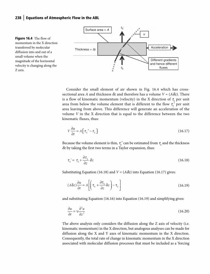
238 Equations of Atmospheric Flow in the ABL
Consider the small element of air shown in Fig. 16.4 which has cross-
sectional area A and thickness dz and therefore has a volume V = (Adz). There
is a flow of kinematic momentum (velocity) in the X direction of tk per unit
area from below the volume element that is different to the flow tk′ per unit
area leaving from above. This difference will generate an acceleration of the
volume V in the X direction that is equal to the difference between the two
kinematic fluxes, thus:
∂ = ′ −⎡ ⎤⎣ ⎦∂ k k
uV A
tt t
(16.17)
Because the volume element is thin, tk′ can be estimated from t
k and the thickness
dz by taking the first two terms in a Taylor expansion, thus:
∂= +
∂' k
k kz
z
tt t d
(16.18)
Substituting Equation (16.18) and V = (Adz) into Equation (16.17) gives:
( ) k
k k
uA z A z
t z
⎡ ⎤∂τ∂ ⎛ ⎞δ = τ + δ − τ⎢ ⎥⎜ ⎟⎝ ⎠∂ ∂⎣ ⎦
(16.19)
and substituting Equation (16.16) into Equation (16.19) and simplifying gives:
2
2
u u
t z
∂ ∂= υ
∂ ∂ (16.20)
The above analysis only considers the diffusion along the Z axis of velocity (i.e.
kinematic momentum) in the X direction, but analogous analyses can be made for
diffusion along the X and Y axes of kinematic momentum in the X direction.
Consequently, the total rate of change in kinematic momentum in the X direction
associated with molecular diffusion processes that must be included as a ‘forcing
Thickness = dz
Surface area = A
Acceleration
Different gradientsand hence different
fluxes
u
tk
tk�
Figure 16.4 The flow of
momentum in the X direction
transferred by molecular
diffusion into and out of a
small volume when the
magnitude of the horizontal
velocity is changing along the
Z axis.
Shuttleworth_c16.indd 238Shuttleworth_c16.indd 238 11/3/2011 6:56:40 PM11/3/2011 6:56:40 PM
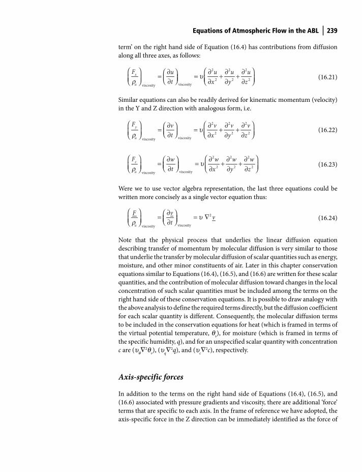
Equations of Atmospheric Flow in the ABL 239
term’ on the right hand side of Equation (16.4) has contributions from diffusion
along all three axes, as follows:
⎛ ⎞ ⎛ ⎞∂ ∂ ∂ ∂⎛ ⎞= = + +⎜ ⎟⎜ ⎟ ⎜ ⎟⎝ ⎠∂ ∂ ∂ ∂⎝ ⎠⎝ ⎠
2 2 2
2 2 2
viscosityviscosity
x
a
F u u u u
t x y zu
r
(16.21)
Similar equations can also be readily derived for kinematic momentum (velocity)
in the Y and Z direction with analogous form, i.e.
⎛ ⎞ ⎛ ⎞∂ ∂ ∂ ∂⎛ ⎞= = + +⎜ ⎟⎜ ⎟ ⎜ ⎟⎝ ⎠∂ ∂ ∂ ∂⎝ ⎠⎝ ⎠
2 2 2
2 2 2
viscosityviscosity
y
a
F v v v v
t x y zu
r
(16.22)
⎛ ⎞ ⎛ ⎞∂ ∂ ∂ ∂⎛ ⎞= = + +⎜ ⎟⎜ ⎟ ⎜ ⎟⎝ ⎠∂ ∂ ∂ ∂⎝ ⎠⎝ ⎠
2 2 2
2 2 2
viscosityviscosity
z
a
F w w w w
t x y zu
r
(16.23)
Were we to use vector algebra representation, the last three equations could be
written more concisely as a single vector equation thus:
⎛ ⎞ ∂⎛ ⎞= = ∇⎜ ⎟⎜ ⎟ ⎝ ⎠∂⎝ ⎠2
viscosityviscosity
a
F vv
tu
r
(16.24)
Note that the physical process that underlies the linear diffusion equation
describing transfer of momentum by molecular diffusion is very similar to those
that underlie the transfer by molecular diffusion of scalar quantities such as energy,
moisture, and other minor constituents of air. Later in this chapter conservation
equations similar to Equations (16.4), (16.5), and (16.6) are written for these scalar
quantities, and the contribution of molecular diffusion toward changes in the local
concentration of such scalar quantities must be included among the terms on the
right hand side of these conservation equations. It is possible to draw analogy with
the above analysis to define the required terms directly, but the diffusion coefficient
for each scalar quantity is different. Consequently, the molecular diffusion terms
to be included in the conservation equations for heat (which is framed in terms of
the virtual potential temperature, qv), for moisture (which is framed in terms of
the specific humidity, q), and for an unspecified scalar quantity with concentration
c are (uq∇2q
v), (u
q∇2q), and (u
c∇2c), respectively.
Axis-specific forces
In addition to the terms on the right hand side of Equations (16.4), (16.5), and
(16.6) associated with pressure gradients and viscosity, there are additional ‘force’
terms that are specific to each axis. In the frame of reference we have adopted, the
axis-specific force in the Z direction can be immediately identified as the force of
Shuttleworth_c16.indd 239Shuttleworth_c16.indd 239 11/3/2011 6:56:44 PM11/3/2011 6:56:44 PM
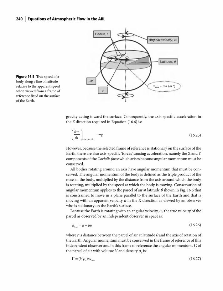
240 Equations of Atmospheric Flow in the ABL
gravity acting toward the surface. Consequently, the axis-specific acceleration in
the Z direction required in Equation (16.6) is:
axis specific
wg
t
∂⎛ ⎞ = −⎜ ⎟∂⎝ ⎠
(16.25)
However, because the selected frame of reference is stationary on the surface of the
Earth, there are also axis-specific ‘forces’ causing acceleration, namely the X and Y
components of the Coriolis force which arises because angular momentum must be
conserved.
All bodies rotating around an axis have angular momentum that must be con-
served. The angular momentum of the body is defined as the triple product of the
mass of the body, multiplied by the distance from the axis around which the body
is rotating, multiplied by the speed at which the body is moving. Conservation of
angular momentum applies to the parcel of air at latitude q shown in Fig. 16.5 that
is constrained to move in a plane parallel to the surface of the Earth and that is
moving with an apparent velocity u in the X direction as viewed by an observer
who is stationary on the Earth’s surface.
Because the Earth is rotating with an angular velocity, ω, the true velocity of the
parcel as observed by an independent observer in space is:
= + ωtrue
u u r
(16.26)
where r is distance between the parcel of air at latitude q and the axis of rotation of
the Earth. Angular momentum must be conserved in the frame of reference of this
independent observer and in this frame of reference the angular momentum, G, of
the parcel of air with volume V and density ra is:
Γ = ( )a true
V rur
(16.27)
wr
Angular velocity, w
Radius, r
Latitude, q
uutrue = u + (w r )
Figure 16.5 True speed of a
body along a line of latitude
relative to the apparent speed
when viewed from a frame of
reference fixed on the surface
of the Earth.
Shuttleworth_c16.indd 240Shuttleworth_c16.indd 240 11/3/2011 6:56:48 PM11/3/2011 6:56:48 PM
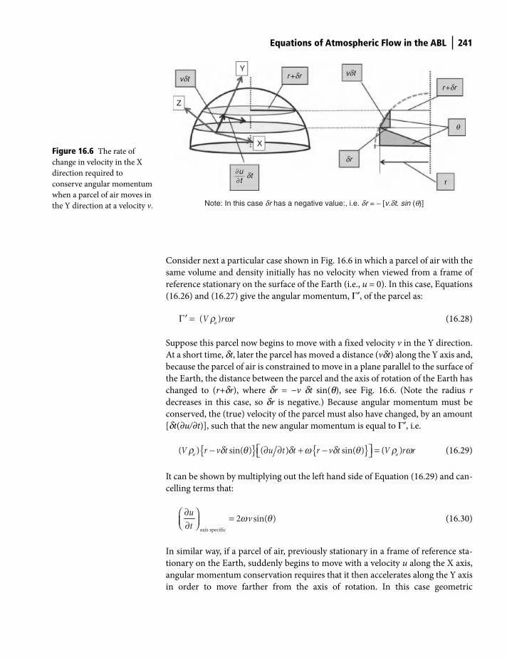
Equations of Atmospheric Flow in the ABL 241
Consider next a particular case shown in Fig. 16.6 in which a parcel of air with the
same volume and density initially has no velocity when viewed from a frame of
reference stationary on the surface of the Earth (i.e., u = 0). In this case, Equations
(16.26) and (16.27) give the angular momentum, Γ′, of the parcel as:
Γ′ = ω ( )a
V r rr
(16.28)
Suppose this parcel now begins to move with a fixed velocity v in the Y direction.
At a short time, dt, later the parcel has moved a distance (vdt) along the Y axis and,
because the parcel of air is constrained to move in a plane parallel to the surface of
the Earth, the distance between the parcel and the axis of rotation of the Earth has
changed to (r+dr), where dr = −v dt sin(q), see Fig. 16.6. (Note the radius r
decreases in this case, so dr is negative.) Because angular momentum must be
conserved, the (true) velocity of the parcel must also have changed, by an amount
[dt(∂u/∂t)], such that the new angular momentum is equal to Γ′, i.e.
{ } { }⎡ ⎤− ∂ ∂ + − =⎣ ⎦( ) sin( ) ( ) sin( ) ( )a a
V r v t u t t r v t V r rr d q d w d q r w
(16.29)
It can be shown by multiplying out the left hand side of Equation (16.29) and can-
celling terms that:
∂⎛ ⎞ =⎜ ⎟⎝ ⎠∂axis specific
2 sin( )u
vt
w q
(16.30)
In similar way, if a parcel of air, previously stationary in a frame of reference sta-
tionary on the Earth, suddenly begins to move with a velocity u along the X axis,
angular momentum conservation requires that it then accelerates along the Y axis
in order to move farther from the axis of rotation. In this case geometric
Z
Y
X
vdtvdt
dr
dt
r +dr
r +dr
r
q
�u�t
Note: In this case dr has a negative value:, i.e. dr = − [v.dt. sin (q)]
Figure 16.6 The rate of
change in velocity in the X
direction required to
conserve angular momentum
when a parcel of air moves in
the Y direction at a velocity v.
Shuttleworth_c16.indd 241Shuttleworth_c16.indd 241 11/3/2011 6:56:51 PM11/3/2011 6:56:51 PM
242 Equations of Atmospheric Flow in the ABL
consideration of the required relationship between the resulting acceleration and
the change in velocity gives:
∂⎛ ⎞ = −⎜ ⎟⎝ ⎠∂axis specific
2 sin( )v
ut
w q
(16.31)
For simplicity when writing Equations (16.30) and (16.31) we have considered
only simple specific cases, but these two equations apply in general and define the
axis-specific forces for the X and Y axes. For consistency with other terms on the
right hand side of Equations (16.4), (16.5) and (16.6), these three equations are
re-written as:
⎛ ⎞=⎜ ⎟⎝ ⎠
axis specific
x
a
Ffv
r
(16.32)
⎛ ⎞= −⎜ ⎟⎝ ⎠
axis specific
y
a
Ffu
r
(16.33)
⎛ ⎞= −⎜ ⎟⎝ ⎠
axis specific
z
a
Fg
r
(16.34)
where:
ω θ= 2 sin( )f
(16.35)
Combined momentum forces
As previously mentioned, to define the equations which together describe the
movement and evolution of momentum in the atmosphere the total rate of change
of momentum along each axis, i.e., Equations (16.4) to (16.6), are combined with
those that describe possible forces that may give rise to change, i.e., Equations
(16.10) to (16.12), Equations (16.21) to (16.23), and Equations (16.32) to (16.34),
as follows:
⎛ ⎞∂ ∂ ∂ ∂ ∂ ∂ ∂ ∂= + + + = − + υ + +⎜ ⎟∂ ∂ ∂ ∂ ∂ ∂ ∂ ∂⎝ ⎠
2 2 2
2 2 2
1
a
du u u u u P u u uu v w fv
dt t x y z x x y zr
(16.36)
⎛ ⎞∂ ∂ ∂ ∂ ∂ ∂ ∂ ∂= + + + = − − + υ + +⎜ ⎟∂ ∂ ∂ ∂ ∂ ∂ ∂ ∂⎝ ⎠
2 2 2
2 2 2
1
a
dv v v v v P v v vu v w fu
dt t x y z y x y zr
(16.37)
⎛ ⎞∂ ∂ ∂ ∂ ∂ ∂ ∂ ∂= + + + = − − + υ + +⎜ ⎟∂ ∂ ∂ ∂ ∂ ∂ ∂ ∂⎝ ⎠
2 2 2
2 2 2
1
a
dw w w w w P w w wu v w g
dt t x y z z x y zr
(16.38)
Shuttleworth_c16.indd 242Shuttleworth_c16.indd 242 11/3/2011 6:56:54 PM11/3/2011 6:56:54 PM
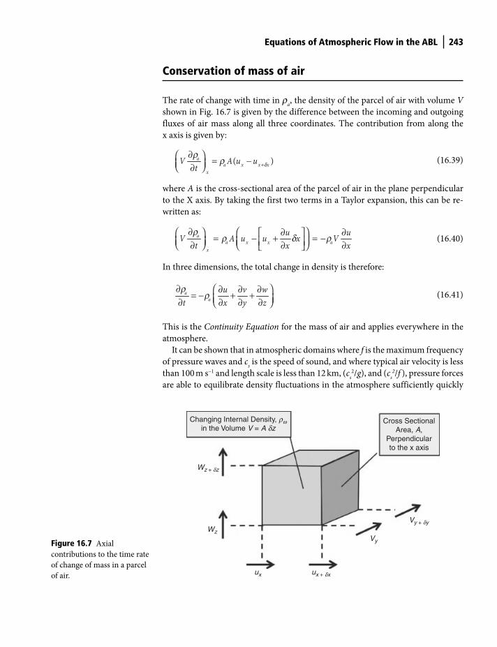
Equations of Atmospheric Flow in the ABL 243
Conservation of mass of air
The rate of change with time in ra, the density of the parcel of air with volume V
shown in Fig. 16.7 is given by the difference between the incoming and outgoing
fluxes of air mass along all three coordinates. The contribution from along the
x axis is given by:
+
∂⎛ ⎞ = −⎜ ⎟⎝ ⎠∂( )a
a x x x
x
V A u ut
d
rr
(16.39)
where A is the cross-sectional area of the parcel of air in the plane perpendicular
to the X axis. By taking the first two terms in a Taylor expansion, this can be re-
written as:
∂ ⎛ ⎞⎛ ⎞ ∂ ∂⎡ ⎤= − + = −⎜ ⎟ ⎜ ⎟⎢ ⎥⎝ ⎠∂ ∂ ∂⎝ ⎠⎣ ⎦a
a x x a
x
u uV A u u x V
t x x
rr d r
(16.40)
In three dimensions, the total change in density is therefore:
⎛ ⎞∂ ∂ ∂ ∂= − + +⎜ ⎟∂ ∂ ∂ ∂⎝ ⎠
a
a
u v w
t x y z
rr
(16.41)
This is the Continuity Equation for the mass of air and applies everywhere in the
atmosphere.
It can be shown that in atmospheric domains where f is the maximum frequency
of pressure waves and cs is the speed of sound, and where typical air velocity is less
than 100 m s−1 and length scale is less than 12 km, (cs2/g), and (c
s2/f ), pressure forces
are able to equilibrate density fluctuations in the atmosphere sufficiently quickly
Changing Internal Density, rwin the Volume V = A dz
Cross SectionalArea, A,
Perpendicularto the x axis
Wz + dz
ux + dx
Vy + dyWz
Vy
ux
Figure 16.7 Axial
contributions to the time rate
of change of mass in a parcel
of air.
Shuttleworth_c16.indd 243Shuttleworth_c16.indd 243 11/3/2011 6:57:02 PM11/3/2011 6:57:02 PM
244 Equations of Atmospheric Flow in the ABL
for the left hand side of Equation (16.41) to be negligible in comparison with the
right hand side. Such conditions apply in the atmospheric boundary layer (ABL).
Consequently in the ABL the continuity equation for mass of air can be simplified
to become:
0u v w
x y z
∂ ∂ ∂+ + =∂ ∂ ∂
(16.42)
This equation can be re-written in the vector format as:
. 0v∇ = (16.43)
Conservation of atmospheric moisture
The time rate of change of the total moisture concentration at a particular point in
the atmosphere is equal to the sum of two terms. The first is the transfer of mois-
ture to that point by molecular transport. This is equivalent to the transfer of a
component of momentum by molecular transfer described earlier and is repre-
sented by including an analogous term in the continuity equation for moisture.
The second contribution is from a source/sink term, Sq
total, that corresponds to the
possible creation or destruction of water molecules by chemical means.
Consequently, the continuity equation for moisture takes the form:
∂ ∂ ∂ ∂+ + +
∂ ∂ ∂ ∂⎛ ⎞∂ ∂ ∂
= υ + +⎜ ⎟∂ ∂ ∂⎝ ⎠
2 2 2
2 2 2 +
total total total total
totaltotal total totalq
q
a
q q q qu v w
t x y z
Sq q q
x y z r
(16.44)
which equation can be written more concisely in vector format as:
∂+ ∇ = υ ∇
∂2. +
totaltotalqtotal total
q
a
Sqv q q
t r
(16.45)
This equation for total moisture might be split into two separate equations which
describe the conservation of water vapor and the conservation of liquid/solid
water (such as cloud droplets) in the atmosphere separately, thus:
⎛ ⎞∂ ∂ ∂ ∂ ∂ ∂ ∂+ + + = υ + +⎜ ⎟∂ ∂ ∂ ∂ ∂ ∂ ∂⎝ ⎠
2 2 2
2 2 2 + +
q v
q
a a
S Eq q q q q q qu v w
t x y z x y z r r
(16.46)
⎛ ⎞∂ ∂ ∂ ∂ ∂ ∂ ∂+ + + = υ + + −⎜ ⎟∂ ∂ ∂ ∂ ∂ ∂ ∂⎝ ⎠
2 2 2
2 2 2 +
ll l l l l l lq v
q
a a
S Eq q q q q q qu v w
t x y z x y z r r
(16.47)
Shuttleworth_c16.indd 244Shuttleworth_c16.indd 244 11/3/2011 6:57:05 PM11/3/2011 6:57:05 PM
Equations of Atmospheric Flow in the ABL 245
where q is the specific humidity of the air, q′ is the liquid/solid water content per
unit mass, Ev is the rate of creation of water vapor by evaporation/sublimation of
liquid/solid water (in kg m−3 sec−1), and Sq and S
ql are possible separate source/
sinks terms (in kg m−3 sec−1) corresponding to chemical formation for vapor and
liquid/solid water, respectively. Equations (16.46) and (16.47) can also be written
more concisely in vector format similar to Equation (16.45), see Table 16.1.
Conservation of energy
The time rate of change of potential temperature of a parcel of air in the atmos-
phere is equal to the sum of three terms, namely, the (by now familiar) rate of
inflow or outflow of thermal energy by molecular transfer processes, energy
entering or leaving the parcel of air as radiation, and energy that is released or
absorbed as a result of phase changes between water vapor and liquid or solid
water within the parcel. Hence, the required equation can be written (for concise-
ness here in vector format) as follows:
θ
λ∂θ+ ∇θ = υ ∇ θ − ∇ −
∂2 1
. v
n
a p a p
Ev R
t c cr r
(16.48)
where Ev is the moisture evaporated within the parcel (in kg m−3 sec−1), l is the
latent heat associated with the phase change from liquid/solid to water vapor, ra
and cp are respectively the density and specific heat at constant pressure of moist
air. In this equation net radiation has three axial components and nR is the net
radiation vector and the second term on the right hand side of Equation (16.48),
the divergence of the net radiation flux, is made up of three terms, one for each axis,
thus;
∂⎡ ⎤∂ ∂∇ + +⎢ ⎥∂ ∂ ∂⎣ ⎦
( )( ) ( )1 1=
n yn x n z
n
a pm a pm
RR RR
c c x y zr r
(16.49)
Among these three terms it is the third, that associated with the vertical flux of
net radiation, which is usually dominant, and in the ABL and over an ‘ideal’
surface, it is assumed that there is no change in horizontal net radiation transfer,
see Equation (5.28).
Conservation of a scalar quantity
The conservation equation for any scalar quantity c (e.g., the concentration of
carbon dioxide) can be written by equating the total derivative of the quantity
to two terms one of which represents the divergence of the flux transferred by
Shuttleworth_c16.indd 245Shuttleworth_c16.indd 245 11/3/2011 6:57:11 PM11/3/2011 6:57:11 PM

246 Equations of Atmospheric Flow in the ABL
molecular transfer while the second represents all possible sources or sinks of
the quantity (which might include chemical reactions that occur at some level
in the atmosphere, as in the case of ozone). Consequently, the general conser-
vation for such scalar quantities (for conciseness here in vector format) takes
the form:
2. q c
cv c c S
t
∂ + ∇ = υ ∇ +∂
(16.50)
Table 16.1 The suite of equations that describe the evolution of atmospheric variables in
the atmosphere.
Ideal Gas Law:
P = raRdTvConservation of mass:
In general In the ABL
ρ ρ ⎛ ⎞∂ ∂ ∂ ∂= − + +⎜ ⎟⎝ ⎠∂ ∂ ∂ ∂a
au v w
t x y z∂ ∂ ∂+ + =∂ ∂ ∂
0u v wx y z
Conservation of momentum:
υρ
⎛ ⎞∂ ∂ ∂ ∂ ∂ ∂ ∂ ∂= + + + = − + + +⎜ ⎟∂ ∂ ∂ ∂ ∂ ∂ ∂ ∂⎝ ⎠
2 2 2
2 2 2
1
a
du u u u u P u u uu v w fv
dt t x y z x x y z
υρ
⎛ ⎞∂ ∂ ∂ ∂ ∂ ∂ ∂ ∂= + + + = − − + + +⎜ ⎟∂ ∂ ∂ ∂ ∂ ∂ ∂ ∂⎝ ⎠
2 2 2
2 2 2
1
a
dv v v v v P v v vu v w fu
dt t x y z y x y z
υρ
⎛ ⎞∂ ∂ ∂ ∂ ∂ ∂ ∂ ∂= + + + = − − + + +⎜ ⎟∂ ∂ ∂ ∂ ∂ ∂ ∂ ∂⎝ ⎠
2 2 2
2 2 2
1
a
dw w w w w P w w wu v w g
dt t x y z z x y z
Conservation of moisture:
υρ ρ
∂ + ∇ = ∇∂
2. + + q vq
a a
Sq Ev q q
t
(vapor)
υρ ρ
∂ + ∇ = ∇ −∂
2. + ll
ql l vq
a a
Sq Ev q q
t (liquid/solid)
Conservation of energy:
θθ λθ υ θ
ρ ρ∂ + ∇ = ∇ − ∇ −∂
2 1. v
na p a p
Ev R
t c c
Conservation of a scalar quantity:
υ∂ + ∇ = ∇ +∂
2. c cc
v c c St
Shuttleworth_c16.indd 246Shuttleworth_c16.indd 246 11/3/2011 6:57:14 PM11/3/2011 6:57:14 PM
Equations of Atmospheric Flow in the ABL 247
Summary of equations of atmospheric flow
In addition to the several conservation equations introduced above, the suite of
basic equations describing the atmosphere also includes the ideal gas law for moist
air here given in terms of virtual temperature (see Equation (2.11) and associated
text), i.e., in the form:
=a d v
P R Tr
(16.51)
where Rd is the gas constant for air (287 J kg K) and T
v = T(1 + 0.61q) is the virtual
temperature. Table 16.1 summarizes the resulting set of equations used to describe
the movement and evolution of atmospheric variables.
Important points in this chapter
● Prognostic equations: the set of equations that describe atmospheric flow at
a point in time, which are often called prognostic equations, are just the local
conservation equations for each atmospheric variable, plus the ideal gas law.
● Time rate of change in fluids: there are two ways in which a property of a mov-
ing fluid measured at a point can change, either in response to mechanisms
acting within the fluid itself (e.g., forces, internal diffusion, or source/sink pro-
cesses), or because the property is not constant with distance inside the fluid
as it moves past the point. Their sum is the total rate of change with time.
● Momentum conservation: the prognostic equations for kinematic velocity
are given by applying momentum conservation equations along three axes,
with the total rate of change of momentum equated to the sum of ‘forces’
associated with pressure gradients, molecular diffusion of momentum, and
axis-specific (Coriolis and gravity) forces.
● Mass conservation: the continuity equation for air mass is given by equating
the local rate of change in air density to the difference between incoming and
outgoing air flow along all three axes. In the ABL, changes in air density
equilibrate quickly (at about the speed of sound) and are often neglected.
● Conservation of other variables: the prognostic equations for other varia-
bles (e.g., moisture, temperature, CO2) are given by equating their total rate
of change to the relevant mechanisms by means of which they might be
changed (e.g., atmospheric sources/sinks, phase changes, radiation
divergence).
Shuttleworth_c16.indd 247Shuttleworth_c16.indd 247 11/3/2011 6:57:24 PM11/3/2011 6:57:24 PM

Introduction
The set of equations which describe the movement and evolution of the atmosphere
in the ABL, at any point in time, were introduced in Chapter 16. In this chapter
these equations are re-written to describe the mean flow for time-average values of
atmospheric variables, including the influence on these mean flow equations of
turbulent fluctuations on the high frequency side of the spectral gap, see Fig. 15.3
and associated text. Doing this involves expressing the value of each variable
described by an equation introduced in Chapter 16 in terms of a mean and a
fluctuating part, then applying the Reynolds averaging rules (see Table 15.2) to
derive the equivalent equation for mean flow, and finally introducing any
simplifications and approximations that are appropriate in the ABL.
Fluctuations in the ideal gas law
Consider first the effect of re-expressing the ideal gas law in terms of atmospheric
variables which recognize mean and fluctuating components. It is convenient to
rearrange the equation P = ra R
d T
v into the form P/R
d = r
aT
v before substituting
P = P—
+ P ', = + ′a a a
r r r and = + ′v v v
T T T to give:
′+ = + ′ + ′ = + ′ + ′ + ′ ′( )( )
a a v v a v v a a v a v
d d
P PT T T T T T
R Rr r r r r r
(17.1)
Averaging this equation it becomes:
′+ = + ′ + ′ + ′ ′
a a a a vv v vd d
P PTT T T
R Rr r r r
(17.2)
17 Equations of Turbulent Flow in the ABL
Terrestrial Hydrometeorology, First Edition. W. James Shuttleworth.
© 2012 John Wiley & Sons, Ltd. Published 2012 by John Wiley & Sons, Ltd.
Shuttleworth_c17.indd 248Shuttleworth_c17.indd 248 11/3/2011 6:54:34 PM11/3/2011 6:54:34 PM
Equations of Turbulent Flow in the ABL 249
and after applying Reynolds averaging to remove the time average of fluctuating
components, the equation reduces to:
= + ′ ′d a d av vP R RT Tr r
(17.3)
However, in practice, ′ ′a vTr is very much less than a v
Tr in the ABL and it can
safely be neglected, consequently:
=v a v
P R Tr
(17.4)
This equation merely says that the ideal gas law applies to average values, which is
as it should be, since it was observation of average values that originally stimulated
its discovery.
It is useful later to subtract Equation (17.3) from Equation (17.2) and then
divide by Equation (17.4) to give:
′ ′′= +a v
a v
TP
P T
rr
(17.5)
In the ABL, pressure fluctuations are rarely if ever observed to be greater than
0.01 kPa and because mean pressure is on the order of 100 kPa, (P/P—
) is on the
order of 10−4. On the other hand, fluctuations in mean temperature, which is itself
on the order of 300 K, are typically on the order of 1 K, hence ( / )v v
T T is on the
order of 33 × 10−4. Consequently it is possible to neglect (P ′/P— ) in comparison with
the other terms and write:
′ ′ ′≈ ≈a v
a v
T
T
r qr q
(17.6)
Using this equation, density fluctuations in the ABL (which are otherwise hard to
measure) can be estimated from the measurable fluctuations in temperature.
The Boussinesq approximation
Starting from the equation for the conservation of momentum in the vertical
direction, Equation (16.38), with the molecular flow term written in vector form
for conciseness, multiplying by ra, recalling m = (r
a u), and then expressing all the
variables as the sum of mean and fluctuating parts gives:
+ ′ ∂ + ′+ ′ = − + ′ − + ∇ + ′
∂2( ) ( )
( ) ( ) ( )a a a a
d w w P Pg w w
dt zr r r r m
(17.7)
Shuttleworth_c17.indd 249Shuttleworth_c17.indd 249 11/3/2011 6:54:39 PM11/3/2011 6:54:39 PM
250 Equations of Turbulent Flow in the ABL
Dividing this last equation by a
r and rearranging gives:
∂ ∂∂ ∂
⎛ ⎞′ ′ ⎛ ⎞+ ′ ′+ = − − − + + ∇ + ′⎜ ⎟⎜ ⎟ ⎝ ⎠⎝ ⎠
2( ) 1 11 ( )a a
a
a a a a
d w w P Pg g w w
dt z z
r rr u
r r r r
(17.8)
The mean vertical pressure gradient in the atmosphere (around which turbulent
fluctuations occur) is in hydrostatic equilibrium, and is described by Equation (3.3).
Consequently the third term on the right hand side of Equation (17.8) is zero.
Equation (17.6) shows that fractional fluctuations in density can be estimated
from fractional fluctuations in temperature, and are of the order 10−2. Fractional
fluctuations in density can therefore be neglected in comparison with unity on
the left hand side of the equation, but must be retained in the first term on the
right hand side of the equation where they can be estimated from temperature
fluctuations. Hence, Equation (17.8) becomes:
∂∂
+ ′ ′ ′= − − + υ∇ + ′2( ) 1
( )a
d w w Pg w w
dt z
qq r
(17.9)
The approximation procedure just used, in which ‘density fluctuations are neglected
in the inertia (storage) term but are retained in the buoyancy term’, is the Boussinesq
approximation. In an equation of atmospheric flow, implementing the Boussinesq
approximation involves simultaneously replacing each occurrence of ra by
ar and
each occurrence of g by g [(r—aa
+ r′a)/r— ] or g[1 − q ′/q
—].
Neglecting subsidence
Observations in the ABL show that the value of w—, the mean vertical wind speed
(which is sometimes referred to as the rate of ‘subsidence’), is usually small and
commonly less than 0.1 m s−1. On the other hand, the magnitude of fluctuations
around this mean value are much greater and on the order of several meters per
second. For this reason it is often assumed acceptable when writing equations
describing momentum conservation to ‘neglect subsidence’, i.e., to retain terms
involving w′ in the equation while removing those involving w—. With this assump-
tion Equation (17.9) would, for example, simplify to:
∂∂
′ ′ ′= − − + ∇ ′21
a
dw Pg w
dt z
qu
q r
(17.10)
Shuttleworth_c17.indd 250Shuttleworth_c17.indd 250 11/3/2011 6:54:47 PM11/3/2011 6:54:47 PM
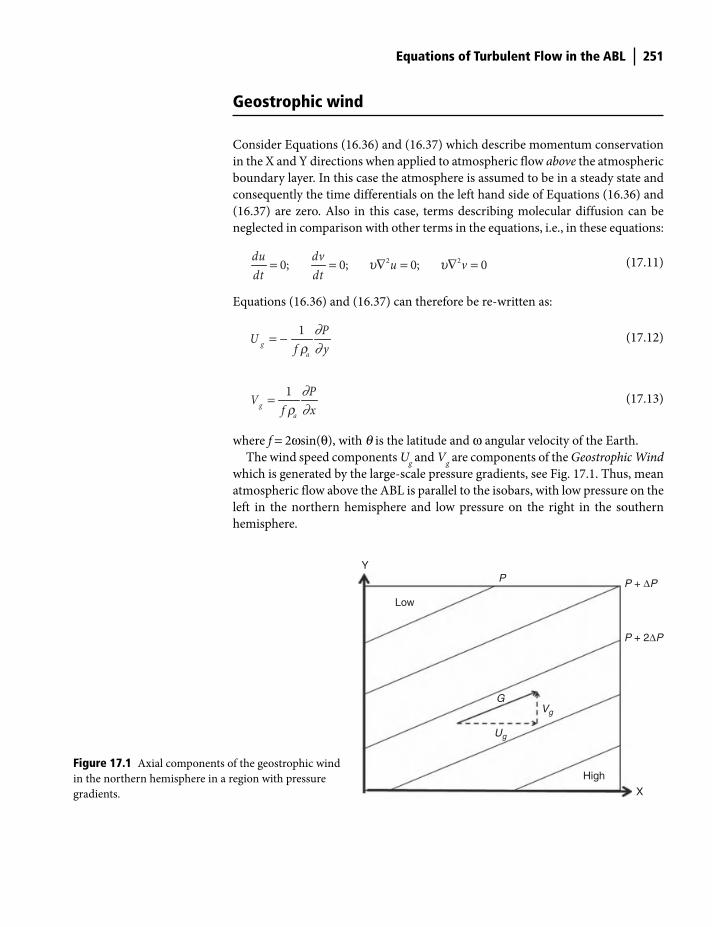
Equations of Turbulent Flow in the ABL 251
Geostrophic wind
Consider Equations (16.36) and (16.37) which describe momentum conservation
in the X and Y directions when applied to atmospheric flow above the atmospheric
boundary layer. In this case the atmosphere is assumed to be in a steady state and
consequently the time differentials on the left hand side of Equations (16.36) and
(16.37) are zero. Also in this case, terms describing molecular diffusion can be
neglected in comparison with other terms in the equations, i.e., in these equations:
= = ∇ = ∇ =2 20; 0; 0; 0du dv
u vdt dt
u u
(17.11)
Equations (16.36) and (16.37) can therefore be re-written as:
∂∂
= −1
g
a
PU
f yr
(17.12)
∂∂
=1
g
a
PV
f xr
(17.13)
where f = 2ωsin(θ), with q is the latitude and ω angular velocity of the Earth.
The wind speed components Ug and V
g are components of the Geostrophic Wind
which is generated by the large-scale pressure gradients, see Fig. 17.1. Thus, mean
atmospheric flow above the ABL is parallel to the isobars, with low pressure on the
left in the northern hemisphere and low pressure on the right in the southern
hemisphere.
Low
High
YP P + ΔP
P + 2ΔP
Vg
Ug
G
X
Figure 17.1 Axial components of the geostrophic wind
in the northern hemisphere in a region with pressure
gradients.
Shuttleworth_c17.indd 251Shuttleworth_c17.indd 251 11/3/2011 6:54:51 PM11/3/2011 6:54:51 PM
252 Equations of Turbulent Flow in the ABL
Divergence equation for turbulent fluctuations
Expressing Equation (16.42), the equation describing the conservation of mass (or
divergence equation) that is relevant in the ABL, in terms of mean and fluctuating
parts gives:
∂ ∂∂ ∂ ∂ ∂ ∂ ∂ ∂∂ ∂ ∂ ∂ ∂ ∂ ∂ ∂ ∂+ ′ + ′ + ′ ′ ′ ′
+ + = + + + + + =( ) ( ) ( )
0u vu u v v w w u v w w
x y z x x y y z z
(17.14)
Averaging, this equation gives:
∂ ∂ ∂ ∂ ∂ ∂∂ ∂ ∂ ∂ ∂ ∂
′ ′ ′+ + + + + = 0
u u v v w w
x x y y z z
(17.15)
From Reynolds averaging rules, the second, fourth, and sixth terms in the last
equation are zero, consequently:
∂ ∂ ∂∂ ∂ ∂
+ + = 0u v w
x y z
(17.16)
While subtracting Equation (17.16) from Equation (17.15) gives the (obvious but
later useful) result:
∂ ∂ ∂∂ ∂ ∂
′ ′ ′+ + = 0
u v w
x y z
(17.17)
Thus, in the ABL the continuity equation holds separately for both the mean and
the fluctuating components of kinematic velocity, i.e., ∇ =. 0u and ∇ ′ =. 0.u
Conservation of momentum in the turbulent ABL
In the following, derivation of the required mean flow equation is illustrated
for the case of the Z axis with those for the X and Y axes then written later by
analogy. Starting from Equation (16.38) and applying the Boussinesq approxima-
tion, gives:
2 2 2
2 2 2
11
w w w w P w w wu v w g
t x y z z x y z
⎛ ⎞′⎛ ⎞+ + + = − − − + υ + +⎜ ⎟ ⎜ ⎟⎝ ⎠ ⎝ ⎠∂ ∂ ∂ ∂ ∂ ∂ ∂ ∂∂ ∂ ∂ ∂ ∂ ∂ ∂ ∂
qrq a
(17.18)
Shuttleworth_c17.indd 252Shuttleworth_c17.indd 252 11/3/2011 6:54:54 PM11/3/2011 6:54:54 PM
Equations of Turbulent Flow in the ABL 253
( ) ( ) ( ) ( ) ( ) ( ) ( )
( ) ( ) ( ) ( )2 2 2
2 2 2
1 1
a
w w w w w w w wu u v v w w
t x y z
P P w w w w w wg
z x y z
+ ′ + ′ + ′ + ′+ + ′ + + ′ + + ′
∂⎛ ⎞+ ′ + ′ + ′ + ′′⎛ ⎞= − − − + + +⎜ ⎟ ⎜ ⎟⎝ ⎠ ⎝ ⎠
∂ ∂ ∂ ∂∂ ∂ ∂
∂ ∂ ∂ ∂∂ ∂ ∂ ∂
q urq
(17.19)
Multiplying out and averaging the last equation, gives:
2 2 2 2 2 2
2 2 2 2 2 2
1 1
a a
w w w w wwu u u u
t t x x x x
w w w w w ww wvv v v w w ww
y y y y z z z z
wP P w w w wwg g
z z x x y y z z
′ ′ ′+ + + + ′ + ′
′ ′ ′ ′+ + + ′ + ′ + + + ′ + ′
⎛ ⎞′ ′ ′ ∂ ′ ∂ ∂ ′= − + − − + + + + + +⎜ ⎟⎝ ⎠
∂ ∂ ∂ ∂ ∂ ∂∂ ∂ ∂ ∂ ∂ ∂
∂ ∂ ∂ ∂ ∂ ∂ ∂ ∂∂ ∂ ∂ ∂ ∂ ∂ ∂ ∂
∂ ∂ ∂ ∂ ∂∂ ∂ ∂ ∂ ∂ ∂ ∂ ∂
q ur rq
(17.20)
Applying Reynolds averaging rules removes terms 2, 4, 5, 8, 9, 12, 13, 16, 18, 20, 22,
and 24 from this equation. Rearranging the remaining terms then gives:
2 2 2
2 2 2
1
a
w w w w P w w w w w wu v w g u v w
t x y z z x y zx y z
⎛ ⎞⎛ ⎞⎛ ⎞ ′ ′ ′+ + + = − − + + + − ′ + ′ + ′⎜ ⎟⎜ ⎟ ⎜ ⎟⎝ ⎠ ⎝ ⎠ ⎝ ⎠∂ ∂ ∂ ∂ ∂ ∂ ∂ ∂ ∂ ∂ ∂∂ ∂ ∂ ∂ ∂ ∂ ∂ ∂∂ ∂ ∂
ur
(17.21)
It is now appropriate to re-write the final term in this last equation so that its
relationship to turbulent fluxes becomes more obvious, as follows.
Multiplying Equation (17.17) by w′ and taking the time average gives:
∂ ∂ ∂∂ ∂ ∂
′ ′ ′′ + ′ + ′ = 0u v w
w w wx y z
(17.22)
Subtracting this zero identity from Equation (17.21) and re-expressing the resulting
equation in more concise form gives:
21
a
w w w u v wdw Pg w u v w w w w
dt z x y z x y z
⎛ ⎞′ ′ ′ ′ ′ ′= − − + ∇ − ′ + ′ + ′ + ′ + ′ + ′⎜ ⎟
⎝ ⎠u
r∂ ∂ ∂ ∂ ∂ ∂∂
∂ ∂ ∂ ∂ ∂ ∂ ∂ (17.23)
Expanding each atmospheric variable in mean and fluctuating parts this becomes:
Shuttleworth_c17.indd 253Shuttleworth_c17.indd 253 11/3/2011 6:55:01 PM11/3/2011 6:55:01 PM
254 Equations of Turbulent Flow in the ABL
The final term in this equation can now be simplified by recognizing that:
∂ ∂∂∂ ∂ ∂
′ ′′ ′= ′ + ′
( ) w uu wu w
x x x
(17.24)
with similar equations relevant for (v′w′) and (w′w′). Consequently Equation
(17.23) can be re-written as:
2( ) ( ) ( )1
a
u w v w w wdw Pg w
dt z x y z
⎛ ⎞′ ′ ′ ′ ′ ′= − − + ∇ − + +⎜ ⎟
⎝ ⎠ur
∂ ∂ ∂∂∂ ∂ ∂ ∂
(17.25)
Starting from the equations describing momentum conservation in the ABL at a
point in time in the X and Y directions (Equations (16.36) and (16.37) ), and
following a procedure similar to that just used for the Z direction above gives:
∂ ∂ ∂∂∂ ∂ ∂ ∂
⎛ ⎞′ ′ ′ ′ ′ ′= − + ∇ − + +⎜ ⎟
⎝ ⎠2
( ) ( ) ( )1
a
u u v u w udu Pf u u
dt x x y zu
r
(17.26)
∂ ∂ ∂ ∂∂ ∂ ∂ ∂
⎛ ⎞′ ′ ′ ′ ′ ′= − − + ∇ − + +⎜ ⎟⎝ ⎠
21 ( ) ( ) ( )
a
dv P u v v v w vf v v
dt y x y zu
r
(17.27)
There are marked similarities between Equations (17.25), (17.26), and (17.27), the
three equations that describe the evolution of mean flow, and Equations (16.36),
(16.37), and (16.38) that describe instantaneous momentum conservation in the
atmosphere. But differences occur because the effect of turbulent fluctuations must
also be considered when describing the variation in mean quantities, and the
additional terms in the mean flow equation account for contributions from turbulent
flux (as opposed to molecular flux) divergence, e.g., the divergence ∂ ∂′ ′( )u w z in
the turbulent momentum flux ′ ′( )u w . If there is coherence between fluctuating
components of velocity these give rise to turbulent fluxes that move momentum
from one place to another, and losses/gains in these fluxes, this will cause acceleration/
deceleration in the mean flow. Table 17.1 gives the physical meaning of the three
equations describing momentum conservation for mean flow in a turbulent field.
Conservation of moisture, heat, and scalars in the turbulent ABL
Starting from the equations for conservation of moisture, heat and scalar quantities
in the atmosphere, and using an approach analogous to that used in the last section
to derive the equations describing conservation of momentum, equivalent mean
flow equations in the ABL can easily be derived. The form of these equations and
the physical meaning of component terms are given in Tables 17.2, 17.3, and 17.4,
respectively.
Shuttleworth_c17.indd 254Shuttleworth_c17.indd 254 11/3/2011 6:55:06 PM11/3/2011 6:55:06 PM
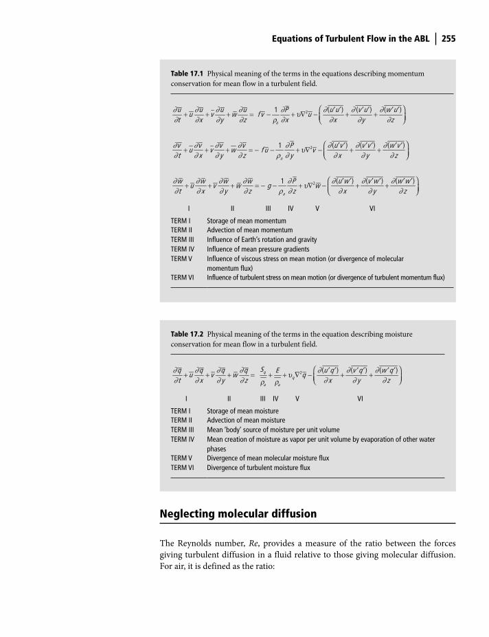
Equations of Turbulent Flow in the ABL 255
Table 17.1 Physical meaning of the terms in the equations describing momentum
conservation for mean flow in a turbulent field.
∂ ∂ ∂ ∂ ∂ ∂ ∂ ∂∂ ∂ ∂ ∂ ∂ ∂ ∂ ∂
⎛ ⎞′ ′ ′ ′ ′ ′+ + + = − + ∇ − + +⎜ ⎟⎝ ⎠21 ( ) ( ) ( )
a
u u u u P u u v u w uu v w f v u
t x y z x x y zu
r
∂ ∂ ∂ ∂ ∂ ∂ ∂ ∂∂ ∂ ∂ ∂ ρ ∂ ∂ ∂ ∂
⎛ ⎞′ ′ ′ ′ ′ ′+ + + = − − + ∇ − + +⎜ ⎟⎝ ⎠21 ( ) ( ) ( )
a
v v v v P u v v v w vu v w f u v
t x y z y x y zu
21 ( ) ( ) ( )
a
w w w w P u w v w w wu v w g w
t x y z z x y z∂ ∂ ∂ ∂ ∂ ∂ ∂ ∂∂ ∂ ∂ ∂ ρ ∂ ∂ ∂ ∂
⎛ ⎞′ ′ ′ ′ ′ ′+ + + = − − + ∇ − + +⎜ ⎟⎝ ⎠u
I II III IV V VI
TERM I Storage of mean momentumTERM II Advection of mean momentumTERM III Influence of Earth’s rotation and gravityTERM IV Influence of mean pressure gradientsTERM V Influence of viscous stress on mean motion (or divergence of molecular
momentum flux)TERM VI Influence of turbulent stress on mean motion (or divergence of turbulent momentum flux)
Table 17.2 Physical meaning of the terms in the equation describing moisture
conservation for mean flow in a turbulent field.
2 ( ) ( ) ( ) q
q
a a
Sq q q q E u q v q w qu v w q
t x y z x y z∂ ∂ ∂ ∂ ∂ ∂ ∂∂ ∂ ∂ ∂ ∂ ∂ ∂
⎛ ⎞′ ′ ′ ′ ′ ′+ + + = + + ∇ − + +⎜ ⎟⎝ ⎠u
r r
I II III IV V VI
TERM I Storage of mean moistureTERM II Advection of mean moistureTERM III Mean ‘body’ source of moisture per unit volumeTERM IV Mean creation of moisture as vapor per unit volume by evaporation of other water
phasesTERM V Divergence of mean molecular moisture fluxTERM VI Divergence of turbulent moisture flux
Neglecting molecular diffusion
The Reynolds number, Re, provides a measure of the ratio between the forces
giving turbulent diffusion in a fluid relative to those giving molecular diffusion.
For air, it is defined as the ratio:
Shuttleworth_c17.indd 255Shuttleworth_c17.indd 255 11/3/2011 6:55:12 PM11/3/2011 6:55:12 PM
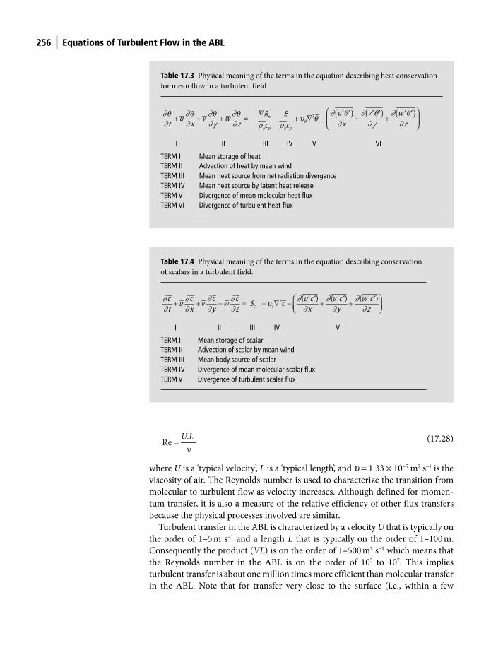
256 Equations of Turbulent Flow in the ABL
Table 17.3 Physical meaning of the terms in the equation describing heat conservation
for mean flow in a turbulent field.
( ) ( ) ( )2 n
a p a p
u v wR Eu v w
t x y z x y zc cθ
∂ θ ∂ θ ∂ θ∂ ∂ ∂ ∂∂ ∂ ∂ ∂ ∂ ∂ ∂ρ ρ
⎛ ⎞′ ′ ′ ′ ′ ′∇+ + + = − − + ∇ − + +⎜ ⎟⎝ ⎠
q q q q u q
I II III IV V VI
TERM I Mean storage of heatTERM II Advection of heat by mean windTERM III Mean heat source from net radiation divergenceTERM IV Mean heat source by latent heat releaseTERM V Divergence of mean molecular heat fluxTERM VI Divergence of turbulent heat flux
Table 17.4 Physical meaning of the terms in the equation describing conservation
of scalars in a turbulent field.
2 ( ) ( ) ( ) c c
c c c c u c v c w cu v w S c
t x y z x y z∂ ∂ ∂ ∂ ∂ ∂ ∂∂ ∂ ∂ ∂ ∂ ∂ ∂
⎛ ⎞′ ′ ′ ′ ′ ′+ + + = + ∇ − + +⎜ ⎟⎝ ⎠u
I II III IV V
TERM I Mean storage of scalarTERM II Advection of scalar by mean windTERM III Mean body source of scalarTERM IV Divergence of mean molecular scalar fluxTERM V Divergence of turbulent scalar flux
=ν.
ReU L
(17.28)
where U is a ‘typical velocity’, L is a ‘typical length’, and u = 1.33 × 10⁻⁵ m2 s−1 is the
viscosity of air. The Reynolds number is used to characterize the transition from
molecular to turbulent flow as velocity increases. Although defined for momen-
tum transfer, it is also a measure of the relative efficiency of other flux transfers
because the physical processes involved are similar.
Turbulent transfer in the ABL is characterized by a velocity U that is typically on
the order of 1–5 m s−1 and a length L that is typically on the order of 1–100 m.
Consequently the product (VL) is on the order of 1–500 m2 s−1 which means that
the Reynolds number in the ABL is on the order of 105 to 107. This implies
turbulent transfer is about one million times more efficient than molecular transfer
in the ABL. Note that for transfer very close to the surface (i.e., within a few
Shuttleworth_c17.indd 256Shuttleworth_c17.indd 256 11/3/2011 6:55:16 PM11/3/2011 6:55:16 PM
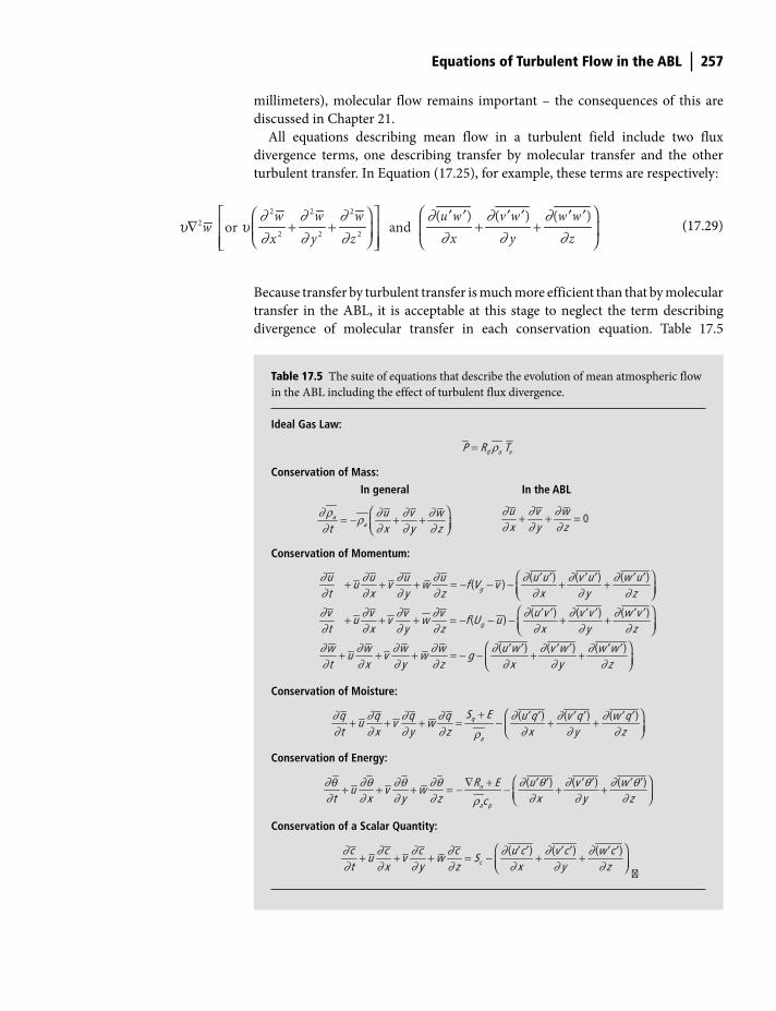
Equations of Turbulent Flow in the ABL 257
millimeters), molecular flow remains important – the consequences of this are
discussed in Chapter 21.
All equations describing mean flow in a turbulent field include two flux
divergence terms, one describing transfer by molecular transfer and the other
turbulent transfer. In Equation (17.25), for example, these terms are respectively:
Table 17.5 The suite of equations that describe the evolution of mean atmospheric flow
in the ABL including the effect of turbulent flux divergence.
Ideal Gas Law:
d a vP R Tρ=
Conservation of Mass:
In general In the ABL
aa
u v wt x y z
∂ ρ ∂ ∂ ∂ρ∂ ∂ ∂ ∂
⎛ ⎞= − + +⎜ ⎟⎝ ⎠
0u v wx y z
∂ ∂ ∂∂ ∂ ∂
+ + =
Conservation of Momentum:
∂ ∂ ∂ ∂ ∂ ∂ ∂∂ ∂ ∂ ∂ ∂ ∂ ∂∂ ∂ ∂ ∂ ∂ ∂ ∂∂ ∂ ∂ ∂ ∂ ∂ ∂∂ ∂ ∂ ∂ ∂ ∂ ∂∂ ∂ ∂ ∂ ∂ ∂ ∂
⎛ ⎞′ ′ ′ ′ ′ ′+ + + = − − − + +⎜ ⎟⎝ ⎠⎛ ⎞′ ′ ′ ′ ′ ′+ + + = − − − + +⎜ ⎟⎝ ⎠
⎛ ′ ′ ′ ′ ′ ′+ + + = − − + +
( ) ( ) ( ) ( )
( ) ( ) ( ) ( )
( ) ( ) ( )
g
g
u u u u u u v u w uu v w f V v
t x y z x y z
v v v v u v v v w vu v w f U u
t x y z x y z
w w w w u w v w w wu v w g
t x y z x y z⎞
⎜ ⎟⎝ ⎠
Conservation of Moisture:
( ) ( ) ( )q
a
S Eq q q q u q v q w qu v w
t x y z x y z∂ ∂ ∂ ∂ ∂ ∂ ∂∂ ∂ ∂ ∂ ∂ ∂ ∂ρ
+ ⎛ ⎞′ ′ ′ ′ ′ ′+ + + = − + +⎜ ⎟⎝ ⎠
Conservation of Energy:
( ) ( ) ( )n
a p
R E u v wu v w
t x y z x y zc
∂ ∂θ ∂θ ∂θ ∂ θ ∂ θ ∂ θ∂ ∂ ∂ ∂ ∂ ∂ ∂ρ
⎛ ⎞∇ + ′ ′ ′ ′ ′ ′+ + + = − − + +⎜ ⎟⎝ ⎠q
Conservation of a Scalar Quantity:
( ) ( ) ( )c
c c c c u c v c w cu v w S
t x y z x y z∂ ∂ ∂ ∂ ∂ ∂ ∂∂ ∂ ∂ ∂ ∂ ∂ ∂
⎛ ⎞′ ′ ′ ′ ′ ′+ + + = − + +⎜ ⎟⎝ ⎠ �
∂ ∂ ∂ ∂ ∂ ∂∂ ∂ ∂∂ ∂ ∂
⎛ ⎞⎡ ⎤⎛ ⎞ ′ ′ ′ ′ ′ ′∇ + + + +⎢ ⎥ ⎜ ⎟⎜ ⎟
⎝ ⎠⎢ ⎥ ⎝ ⎠⎣ ⎦
2 2 2
2
2 2 2
( ) ( ) ( ) or and
w w w u w v w w ww
x y zx y zu u (17.29)
Because transfer by turbulent transfer is much more efficient than that by molecular
transfer in the ABL, it is acceptable at this stage to neglect the term describing
divergence of molecular transfer in each conservation equation. Table 17.5
Shuttleworth_c17.indd 257Shuttleworth_c17.indd 257 11/3/2011 6:55:18 PM11/3/2011 6:55:18 PM

258 Equations of Turbulent Flow in the ABL
summarizes the resulting set of equations used to describe the movement and
evolution of mean flow in the atmosphere.
Important points in this chapter
● Derivation methodology: turbulent flow equations are all derived by express-
ing variables as turbulent fluctuations superimposed on mean values and
then using Reynolds averaging rules to remove terms with zero time-average
value.
● Simplifying assumptions: often used in the ABL are:
– a v a vT T′ ′ <<r r in the ideal gas law;
– density fluctuations can be estimated from ( / ) ( / )aa′ ≈ ′rr q q ;
– (1 )aa+ ′ rr = 1 in the Boussinesq approximation;
– subsidence can often be neglected (i.e., w— ≈ 0) because |w—| << |w'|
● Geostrophic wind: because the free atmosphere above the ABL is in a steady
state, time differentials in equations describing u and v are zero and the wind
components are Ug = −(2r
aw.sin(q) )−1 (∂P/∂ y) and V
g = (2r
aw.sin(q) )−1
(∂P/∂ x).
● Divergence equation: the continuity equation in the ABL holds for both the
mean and fluctuating components of kinematic velocity, i.e., ∇ =. 0u and
∇ ′ =. 0.u
● Turbulent flux divergence: in all equations describing mean atmospheric
flow in a turbulent field the divergence of fluxes transferred by turbulent
flow must be included in addition to the divergence of fluxes transferred by
molecular flow.
● Prognostic equations: prognostic equations for mean atmospheric flow are
all similar to those for instantaneous atmospheric flow, but they include extra
terms describing turbulent flux divergence (Tables 17.1, 17.2, 17.3, and 17.4).
● Neglecting molecular flow: turbulent transfer is about a million times more
efficient than molecular transfer in the ABL, so it is acceptable to neglect the
divergence of molecular transfer fluxes in prognostic equations for mean flow.
Shuttleworth_c17.indd 258Shuttleworth_c17.indd 258 11/3/2011 6:55:26 PM11/3/2011 6:55:26 PM
Introduction
The equations describing the evolution of the mean values of atmospheric variables
in the turbulent ABL were introduced in Chapter 17. It is appropriate next to
investigate how these equations control atmospheric behavior by considering
typical observed changes in mean variables and turbulent fluxes in the ABL during
the course of the day. For simplicity, it is helpful to do this while assuming the ABL
overlies a flat, horizontally homogeneous surface. This makes the equations
simpler to understand because it means terms that represent the rate of change of
mean values or turbulent fluxes with distance along the X and Y axes can be
assumed small in comparison with those that describe the rate of change along the
Z axis. If the terrain is flat, it is also plausible to assume that the mean wind speed
along the Z axis (i.e., subsidence) is zero.
Nature and evolution of the ABL
In general terms, the lower atmosphere can be divided into the four main layers
which are diagnosed by the rate of change with height of virtual potential
temperature, wind speed, specific humidity and other scalar variables, as shown
in Fig. 18.1 for daytime conditions. The lowest layer, the surface layer, which has a
depth on the order of 100 meters, is strongly influenced by the aerodynamic
roughness of the underlying surface and by surface heating. In this layer, mean
atmospheric variables initially change rapidly with height but the rate of change
becomes progressively less away from the surface. During the day, air in the surface
layer is usually unstable because of surface warming but at night the surface layer
usually becomes stable as the surface cools by emitting longwave radiation.
18 Observed ABL Profiles: Higher Order Moments
Terrestrial Hydrometeorology, First Edition. W. James Shuttleworth.
© 2012 John Wiley & Sons, Ltd. Published 2012 by John Wiley & Sons, Ltd.
Shuttleworth_c18.indd 259Shuttleworth_c18.indd 259 11/3/2011 6:53:34 PM11/3/2011 6:53:34 PM
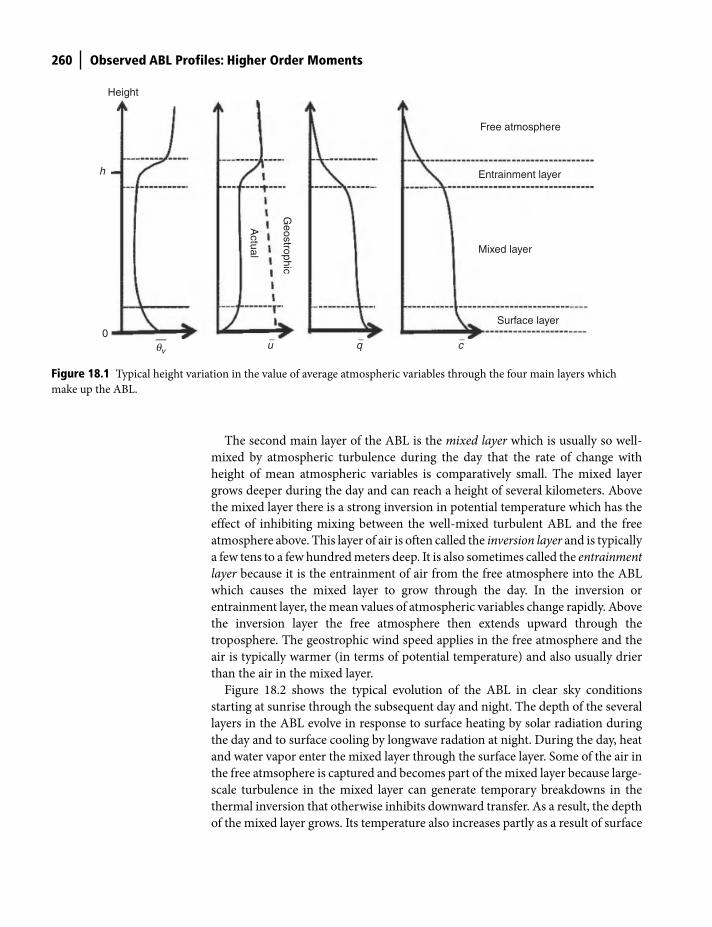
260 Observed ABL Profiles: Higher Order Moments
The second main layer of the ABL is the mixed layer which is usually so well-
mixed by atmospheric turbulence during the day that the rate of change with
height of mean atmospheric variables is comparatively small. The mixed layer
grows deeper during the day and can reach a height of several kilometers. Above
the mixed layer there is a strong inversion in potential temperature which has the
effect of inhibiting mixing between the well-mixed turbulent ABL and the free
atmosphere above. This layer of air is often called the inversion layer and is typically
a few tens to a few hundred meters deep. It is also sometimes called the entrainment
layer because it is the entrainment of air from the free atmosphere into the ABL
which causes the mixed layer to grow through the day. In the inversion or
entrainment layer, the mean values of atmospheric variables change rapidly. Above
the inversion layer the free atmosphere then extends upward through the
troposphere. The geostrophic wind speed applies in the free atmosphere and the
air is typically warmer (in terms of potential temperature) and also usually drier
than the air in the mixed layer.
Figure 18.2 shows the typical evolution of the ABL in clear sky conditions
starting at sunrise through the subsequent day and night. The depth of the several
layers in the ABL evolve in response to surface heating by solar radiation during
the day and to surface cooling by longwave radation at night. During the day, heat
and water vapor enter the mixed layer through the surface layer. Some of the air in
the free atmsophere is captured and becomes part of the mixed layer because large-
scale turbulence in the mixed layer can generate temporary breakdowns in the
thermal inversion that otherwise inhibits downward transfer. As a result, the depth
of the mixed layer grows. Its temperature also increases partly as a result of surface
Height
h
0
Actual
Geostrophic
Free atmosphere
Entrainment layer
Mixed layer
Surface layer
q—v
u� q� c�
Figure 18.1 Typical height variation in the value of average atmospheric variables through the four main layers which
make up the ABL.
Shuttleworth_c18.indd 260Shuttleworth_c18.indd 260 11/3/2011 6:53:35 PM11/3/2011 6:53:35 PM
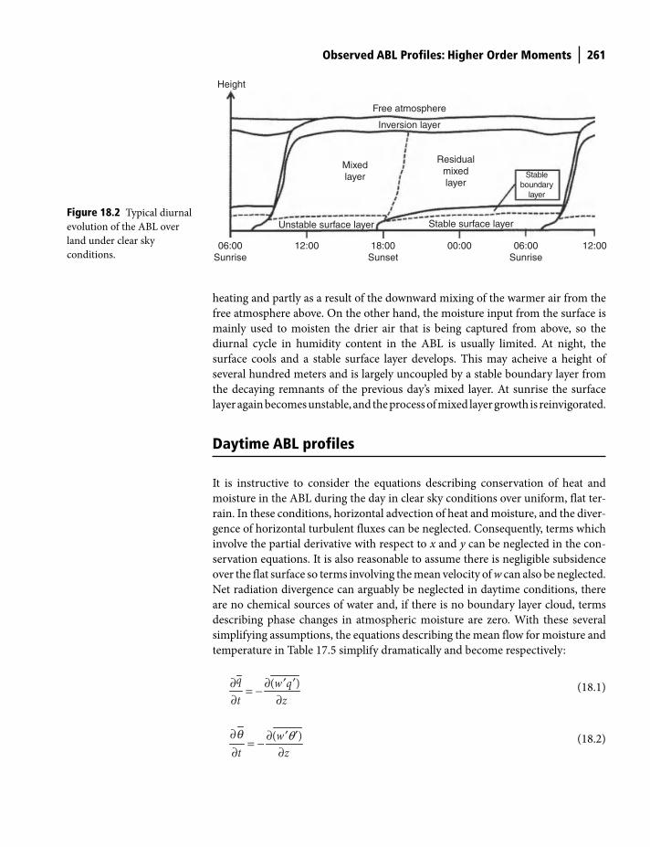
Observed ABL Profiles: Higher Order Moments 261
heating and partly as a result of the downward mixing of the warmer air from the
free atmosphere above. On the other hand, the moisture input from the surface is
mainly used to moisten the drier air that is being captured from above, so the
diurnal cycle in humidity content in the ABL is usually limited. At night, the
surface cools and a stable surface layer develops. This may acheive a height of
several hundred meters and is largely uncoupled by a stable boundary layer from
the decaying remnants of the previous day’s mixed layer. At sunrise the surface
layer again becomes unstable, and the process of mixed layer growth is reinvigorated.
Daytime ABL profiles
It is instructive to consider the equations describing conservation of heat and
moisture in the ABL during the day in clear sky conditions over uniform, flat ter-
rain. In these conditions, horizontal advection of heat and moisture, and the diver-
gence of horizontal turbulent fluxes can be neglected. Consequently, terms which
involve the partial derivative with respect to x and y can be neglected in the con-
servation equations. It is also reasonable to assume there is negligible subsidence
over the flat surface so terms involving the mean velocity of w can also be neglected.
Net radiation divergence can arguably be neglected in daytime conditions, there
are no chemical sources of water and, if there is no boundary layer cloud, terms
describing phase changes in atmospheric moisture are zero. With these several
simplifying assumptions, the equations describing the mean flow for moisture and
temperature in Table 17.5 simplify dramatically and become respectively:
∂ ∂ ′ ′= −∂ ∂
( )q w qt z
(18.1)
( )wt z
∂ ∂ ′ ′= −∂ ∂
θq (18.2)
06:00Sunrise
Height
Mixedlayer
Free atmosphere
Inversion layer
Residualmixedlayer
Stableboundary
layer
Unstable surface layer Stable surface layer
18:00Sunset
12:00 06:00Sunrise
12:0000:00
Figure 18.2 Typical diurnal
evolution of the ABL over
land under clear sky
conditions.
Shuttleworth_c18.indd 261Shuttleworth_c18.indd 261 11/3/2011 6:53:35 PM11/3/2011 6:53:35 PM
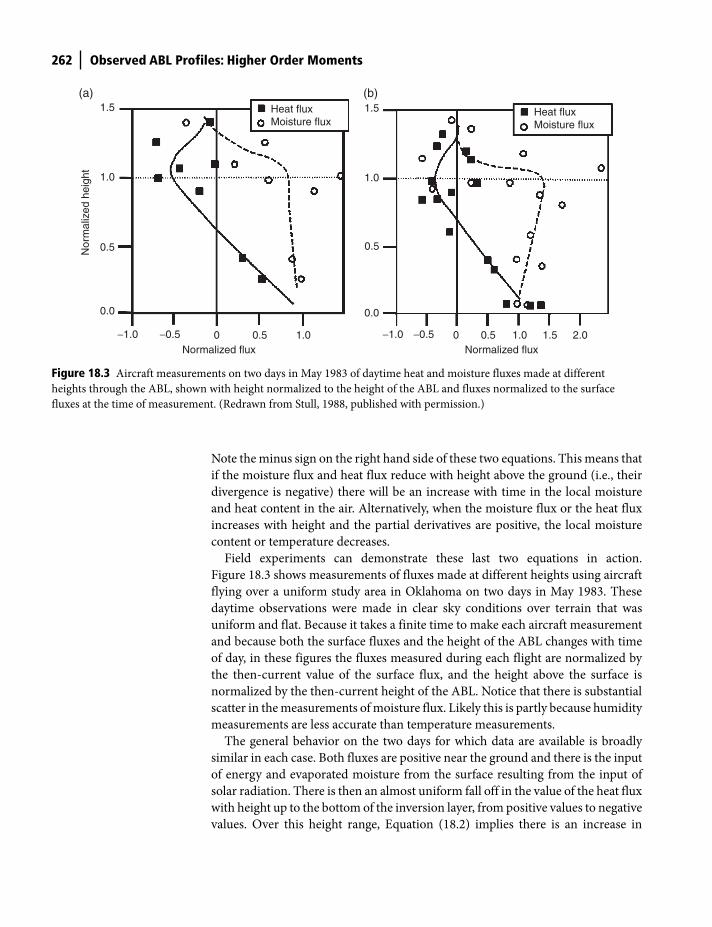
262 Observed ABL Profiles: Higher Order Moments
Note the minus sign on the right hand side of these two equations. This means that
if the moisture flux and heat flux reduce with height above the ground (i.e., their
divergence is negative) there will be an increase with time in the local moisture
and heat content in the air. Alternatively, when the moisture flux or the heat flux
increases with height and the partial derivatives are positive, the local moisture
content or temperature decreases.
Field experiments can demonstrate these last two equations in action.
Figure 18.3 shows measurements of fluxes made at different heights using aircraft
flying over a uniform study area in Oklahoma on two days in May 1983. These
daytime observations were made in clear sky conditions over terrain that was
uniform and flat. Because it takes a finite time to make each aircraft measurement
and because both the surface fluxes and the height of the ABL changes with time
of day, in these figures the fluxes measured during each flight are normalized by
the then-current value of the surface flux, and the height above the surface is
normalized by the then-current height of the ABL. Notice that there is substantial
scatter in the measurements of moisture flux. Likely this is partly because humidity
measurements are less accurate than temperature measurements.
The general behavior on the two days for which data are available is broadly
similar in each case. Both fluxes are positive near the ground and there is the input
of energy and evaporated moisture from the surface resulting from the input of
solar radiation. There is then an almost uniform fall off in the value of the heat flux
with height up to the bottom of the inversion layer, from positive values to negative
values. Over this height range, Equation (18.2) implies there is an increase in
(a) (b)
−1.0
0.0
Normalized flux
Nor
mal
ized
hei
ght
0.5
1.0
1.5 Heat fluxMoisture flux
−0.5 0.5 1.00 −1.0
0.0
Normalized flux
0.5
1.0
1.5 Heat fluxMoisture flux
−0.5 0.5 1.0 1.5 2.00
Figure 18.3 Aircraft measurements on two days in May 1983 of daytime heat and moisture fluxes made at different
heights through the ABL, shown with height normalized to the height of the ABL and fluxes normalized to the surface
fluxes at the time of measurement. (Redrawn from Stull, 1988, published with permission.)
Shuttleworth_c18.indd 262Shuttleworth_c18.indd 262 11/3/2011 6:53:38 PM11/3/2011 6:53:38 PM
Observed ABL Profiles: Higher Order Moments 263
temperature with time that is almost independent of height, consistent with the
fact that there is a well-mixed atmosphere over this height range. The heat flux
changes sign through the mixed layer revealing that this ABL warming is supported
partly by upward heat from the ground at lower levels and partly by downward
heat in the warm air entrained from above the inversion layer at higher levels. The
heat flux remains negative (i.e., downward) through and just above the inversion,
but the rate of change in heat flux becomes positive. Equation (18.2) therefore
implies that at these levels the air that is being entrained from the overlying free
atmosphere is cooling as it merges with the cooler air in the growing mixed layer.
The behavior of the moisture flux is less well-illustrated by the data, but is clearly
very different. The moisture flux remains positive through the mixed layer and
then falls off progressively through and just above the inversion layer. The change
in moisture flux with height through the mixed layer is small (slightly negative on
one day and slightly positive on the second day), so Equation (18.1) implies there is
only modest change in moisture content with time. Through and just above the
inversion layer, the moisture flux remains positive, but it falls rapidly. At these levels
moisture from the surface, which has largely passed straight through the mixed
layer, is used to moisten the drier free atmosphere air as it is entrained downward
to become part of the growing mixed layer.
In summary, the behavior of observed fluxes through and above the evolving
daytime boundary layer shows boundary layer growth involves inputs from both
below and above the inversion layer. Growth is achieved by entraining air from the
free atmosphere which is warmer and drier than the air already in the mixed layer.
Moisture that entered the mixed layer from below is largely used to moisten the
dry entrained air. Hence, the humidity of the air in the ABL is often reasonably
constant through the day. On the other hand, sensible heat is brought into the ABL
from both below and above, and there is a significant diurnal cycle in ABL
temperature during the day. This comparatively simple model of boundary layer
growth over flat uniform terrain can be modeled quite well. Figure 18.4a, for
example, shows the modeled time evolution of profiles of potential temperature,
which can be compared with observed profiles measured at Wangara, Australia on
a day in 1967, shown in Fig. 18.4b. Figure 18.4c shows modeled profiles of humidity
on the same day which can be compared with the observed profiles shown in
Fig. 18.4d.
Nighttime ABL profiles
At night, turbulence in the ABL declines and other terms in the equations
describing the mean flow remain significant in comparison. Over uniform flat
terrain the rate of change of mean values or turbulent fluxes with distance along
the X and Y axes can still be assumed to be small, but subsidence (the mean wind
speed along the Z axis) cannot necessarily be assumed to be zero. Also, because
the net radiation is now all longwave radiation, temperature variation with height
Shuttleworth_c18.indd 263Shuttleworth_c18.indd 263 11/3/2011 6:53:38 PM11/3/2011 6:53:38 PM
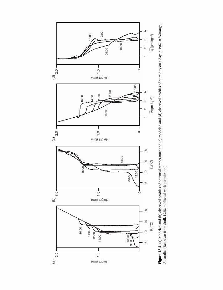
Figu
re 1
8.4
(a)
Mo
del
ed a
nd
(b
) o
bse
rved
pro
file
s o
f p
ote
nti
al t
emp
erat
ure
an
d (
c) m
od
eled
an
d (
d)
ob
serv
ed p
rofi
les
of
hu
mid
ity
on
a d
ay i
n 1
96
7 a
t W
aran
ga,
Au
stra
lia.
(R
edra
wn
fro
m S
tull
, 19
88
, pu
bli
shed
wit
h p
erm
issi
on
.)
6
0
1.0
2.0
0
1.0
2.0
Height (km)
Height (km)
1014
186
1014
18
18:0
0
09:0
0 12:0
015:0
016
:00
14:0
0
12:0
0
11:0
0
10:0
009
:00
(b)
(a)
q�
v (�
C)
q�
v (�
C)
0
1.0
2.0
Height (km)
0
1.0
2.0
Height (km)
12
34
12
18:0
0
10:0
0
11:0
0
12:0
0
14:0
0
16:0
0
09:0
009
:00
12:0
0
15:0
0
(d)
(c)
34
q�
(gm
kg
−1)
q�
(gm
kg
−1)
Shuttleworth_c18.indd 264Shuttleworth_c18.indd 264 11/3/2011 6:53:38 PM11/3/2011 6:53:38 PM
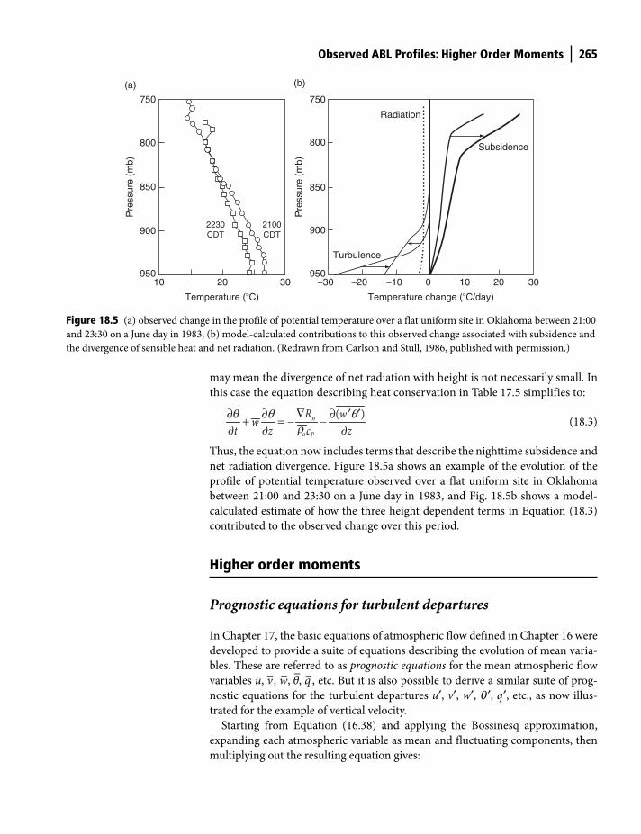
Observed ABL Profiles: Higher Order Moments 265
may mean the divergence of net radiation with height is not necessarily small. In
this case the equation describing heat conservation in Table 17.5 simplifies to:
( )n
pa
R ww
t z zc∇∂ ∂ ∂ ′ ′+ = − −
∂ ∂ ∂θ θq
r (18.3)
Thus, the equation now includes terms that describe the nighttime subsidence and
net radiation divergence. Figure 18.5a shows an example of the evolution of the
profile of potential temperature observed over a flat uniform site in Oklahoma
between 21:00 and 23:30 on a June day in 1983, and Fig. 18.5b shows a model-
calculated estimate of how the three height dependent terms in Equation (18.3)
contributed to the observed change over this period.
Higher order moments
Prognostic equations for turbulent departures
In Chapter 17, the basic equations of atmospheric flow defined in Chapter 16 were
developed to provide a suite of equations describing the evolution of mean varia-
bles. These are referred to as prognostic equations for the mean atmospheric flow
variables ū, v−, w−, −θ, q−, etc. But it is also possible to derive a similar suite of prog-
nostic equations for the turbulent departures u′, v′, w′, q ′, q′, etc., as now illus-
trated for the example of vertical velocity.
Starting from Equation (16.38) and applying the Bossinesq approximation,
expanding each atmospheric variable as mean and fluctuating components, then
multiplying out the resulting equation gives:
−30950
900
850
800
750
950
900
850
800
750
−20 −10 10 20 3020 3010 0
Turbulence
Temperature change (�C/day)Temperature (�C)
(a) (b)
Pre
ssur
e (m
b)
Pre
ssur
e (m
b)
Subsidence
Radiation
2100CDT
2230CDT
Figure 18.5 (a) observed change in the profile of potential temperature over a flat uniform site in Oklahoma between 21:00
and 23:30 on a June day in 1983; (b) model-calculated contributions to this observed change associated with subsidence and
the divergence of sensible heat and net radiation. (Redrawn from Carlson and Stull, 1986, published with permission.)
Shuttleworth_c18.indd 265Shuttleworth_c18.indd 265 11/3/2011 6:53:39 PM11/3/2011 6:53:39 PM
266 Observed ABL Profiles: Higher Order Moments
to give the result:
Subtracting from this last equation the prognostic equation for mean vertical wind
speed given in Table 17.5 gives:
∂ ∂ ′ ∂ ∂ ′ ∂ ∂ ′ ∂ ∂ ′ ∂ ∂ ′+ + + + ′ + ′ + + + ′ + ′
∂ ∂ ∂ ∂ ∂ ∂ ∂ ∂ ∂ ∂′∂ ∂ ′ ∂ ∂ ′ ∂ ∂ ′
+ + + ′ + ′ = − + − −ρ ρ∂ ∂ ∂ ∂ ∂ ∂
⎛ ⎞∂ ∂ ′ ∂ ∂ ′ ∂ ∂ ′+ + + + + +⎜ ⎟∂ ∂ ∂ ∂ ∂ ∂⎝ ⎠
2 2 2 2 2 2
2 2 2 2 2 2
1 1v
a av
w w w w w w w w w wu u u u v vv vt t x x x x y y y y
w w w w PPw w w w g gz z z z z z
w w w w w wx x y y z z
θθ
υ
(18.4)
Using essentially the same procedure as above, similar prognostic equations can
be derived for turbulent fluctuations in other velocity components.
Equation (18.5) is the short-lived prognostic equation for the fluctuation w′. In
principle, it might be used in a short time-step model of turbulence. However, in
such basic form prognostic equations of turbulent fluctuations have limited value
because their descriptive ability is limited to the time of existence of a turbulent
eddy. However, the equations can be used to derive prognostic equations for
turbulent variance. Again their derivation is illustrated by example for the case of
variance in vertical velocity.
The first step is to multiply Equation (18.5) by 2w′ and then to collect terms
using the relationships:
( ) ( ) ( )2 2 2
2 2 2
1 v
av
w w w w w w w w w wu w u v w u v wvt x y z x y z x y z
u w v w w wP w w wgz x y zx y z
⎛ ⎞⎛ ⎞ ⎛ ⎞∂ ′ ∂ ′ ∂ ′ ∂ ′ ∂ ∂ ∂ ∂ ′ ∂ ′ ∂ ′+ + + + ′ + ′ + ′ + ′ + ′ + ′⎜ ⎟⎜ ⎟ ⎜ ⎟∂ ∂ ∂ ∂ ∂ ∂ ∂ ∂ ∂ ∂⎝ ⎠ ⎝ ⎠⎝ ⎠⎛ ⎞∂ ′ ′ ∂ ′ ′ ∂ ′ ′⎛ ⎞′ ∂ ′ ∂ ′ ∂ ′ ∂ ′= − + + + + + +⎜ ⎟⎜ ⎟∂ ∂ ∂ ∂∂ ∂ ∂⎝ ⎠ ⎝ ⎠
qu
rq
(18.5)
∂ ′ ∂ ′ ∂ ′ ∂ ′ ∂ ′ ∂ ′ ∂ ′ ∂ ′= ′ = ′ = ′ = ′∂ ∂ ∂ ∂ ∂ ∂ ∂ ∂
2 2 2 2( ) ( ) ( ) ( )2 ; 2 ; 2 ; 2
w w w w w w w ww w w wt t x x y y z z
(18.6)
⎛ ⎞⎛ ⎞∂ ′ ∂ ′ ∂ ′ ∂ ′ ∂ ∂ ∂+ + + + ′ ′ + ′ ′ + ′ ′⎜ ⎟⎜ ⎟∂ ∂ ∂ ∂ ∂ ∂ ∂⎝ ⎠ ⎝ ⎠
⎛ ⎞ ′∂ ′ ∂ ′ ∂ ′ ∂ ′+ ′ + ′ + ′ = ′ − ′⎜ ⎟∂ ∂ ∂ ∂⎝ ⎠
⎛ ⎞∂ ′ ∂ ′ ∂ ′ ∂ ′ ′ ∂ ′ ′+ ′ + + + ′ +⎜ ⎟ ∂∂ ∂ ∂⎝ ⎠
2 2 2 2
2 2 2
2 2 2
2 2 2
( ) ( ) ( ) ( )2 2 2
( ) ( ) ( ) 1 2 2
( ) ( ) 2 2
v
av
w w w w w w wu v w w u w v w wt x y z x y z
w w w Pu v w w g wx y z z
w w w u w v ww wxx y z
qrq
u⎛ ⎞∂ ′ ′
+⎜ ⎟∂ ∂⎝ ⎠( )w w
y z
(18.7)
Shuttleworth_c18.indd 266Shuttleworth_c18.indd 266 11/3/2011 6:53:40 PM11/3/2011 6:53:40 PM
Observed ABL Profiles: Higher Order Moments 267
The last term disappears on taking the time average of this last equation and
applying Reynolds averaging rules, and the equation then becomes:
⎛ ⎞ ⎛ ⎞∂ ′ ∂ ′ ∂ ′ ∂ ′ ∂ ∂ ∂+ + + + ′ ′ + ′ ′ + ′ ′⎜ ⎟ ⎜ ⎟∂ ∂ ∂ ∂ ∂ ∂ ∂⎝ ⎠⎝ ⎠
⎛ ⎞ ′ ′∂ ′ ∂ ′ ∂ ′ ∂ ′⎛ ⎞+ ′ + ′ + ′ = − ′⎜ ⎟ ⎜ ⎟⎝ ⎠∂ ∂ ∂ ∂⎝ ⎠
+
2 2 2 2
2 2 2
( ) ( ) ( ) ( )2( ) 2( ) 2( )
( )( ) ( ) ( ) 2 2
2
v
av
w w w w w w wu v w w u w v w wt x y z x y z
ww w w Pu v w g wx y z z
qrq
⎛ ⎞′∂ ′ ∂ ∂ ′′ + ′ + ′⎜ ⎟∂ ∂ ∂⎝ ⎠
2 2 2
2 2 2
ww ww w wx y z
u
(18.8)
Recall that the divergence of turbulent fluctuations is zero in the ABL. Consequently
Equation (18.8) still holds if the time average of the product of (w′)2 with the diver-
gence of turbulent fluctuations is added into the left hand side of Equation (18.8).
When this is done, the equation becomes:
⎛ ⎞ ⎛ ⎞∂ ′ ∂ ′ ∂ ′ ∂ ′ ∂ ∂ ∂+ + + + ′ ′ + ′ ′ + ′ ′⎜ ⎟ ⎜ ⎟∂ ∂ ∂ ∂ ∂ ∂ ∂⎝ ⎠⎝ ⎠
⎛ ⎞∂ ∂ ∂′ ′ ′∂ ′ ∂ ′ ∂ ′ + ′ + ′ + ′+ ′ + ′ + ′⎜ ⎟∂ ∂ ∂∂ ∂ ∂⎝ ⎠′ ′ ∂ ′
= − ′∂
2 2 2 2
2 2 22 2 2
( ) ( ) ( ) ( )2( ) 2( ) 2( )
( ) ( ) ( ) ( ) ( ) ( )
( ) 22
v
av
w w w w w w ww w u w v w wvut x y z x y z
u v uw w w w w wu v w x x xx y zw Pg wq
rq⎛ ⎞⎛ ⎞ ′∂ ′ ∂ ∂ ′⎜ ⎟ + ′ + ′ + ′⎜ ⎟⎝ ⎠ ∂ ∂ ∂⎝ ⎠
2 2 2
2 2 22
ww ww w wz x y zu
(18.9)
The product rule of calculus gives the four identities:
∂ ′ ′ ∂ ′ ∂ ′= ′ + ′∂ ∂ ∂
∂ ′ ′ ∂ ′ ∂ ′= ′ + ′∂ ∂ ∂
∂ ′ ′ ∂ ′ ∂ ′= ′ + ′∂ ∂ ∂
∂ ′ ′ ∂ ′ ∂ ′= ′ + ′∂ ∂ ∂
2 22
2 22
2 22
( ) ( )( )
( ) ( )( )
( ) ( )( )
( )
u w w uu wx x x
v w w vv wy y y
w w w ww wz z z
w P P ww Pz z z
(18.10)
Shuttleworth_c18.indd 267Shuttleworth_c18.indd 267 11/3/2011 6:53:44 PM11/3/2011 6:53:44 PM
268 Observed ABL Profiles: Higher Order Moments
Using the first three identities in the fourth term of Equation (18.8) and
rearranging gives:
⎛ ⎞ ′ ′∂ ′ ∂ ′ ∂ ′ ∂ ′ ∂ ′ ′ ∂ ′+ + + = − + ′⎜ ⎟∂ ∂ ∂ ∂ ∂ ∂⎝ ⎠
⎛ ⎞⎛ ⎞∂ ∂ ∂ ∂ ′ ′ ∂ ′ ′ ∂ ′ ′− ′ ′ + ′ ′ + ′ ′ − + +⎜ ⎟⎜ ⎟∂ ∂ ∂ ∂ ∂ ∂⎝ ⎠ ⎝ ⎠
⎛ ⎞∂ ′ ∂ ′ ∂ ′+ ′ + ′ + ′⎜ ⎟∂ ∂ ∂⎝ ⎠
2 2 2 2
2 2 2
2 2 2
2 2 2
( )( ) ( ) ( ) ( ) 2 ( ) 22
( ) ( ) ( )2( ) 2( ) 2( )
2
v
a av
ww w w w w P wu v w g Pt x y z z z
w w w u w v w w ww u w v w wx y z x y z
w w ww w wx y z
qr rq
u
(18.11)
The product rule of calculus gives the results:
∂ ′ ∂ ′ ∂ ′⎛ ⎞= ′ + ⎜ ⎟⎝ ⎠∂ ∂∂⎛ ⎞∂ ′ ∂ ′ ∂ ′= ′ + ⎜ ⎟∂ ∂∂ ⎝ ⎠
∂ ′ ∂ ′ ∂ ′⎛ ⎞= ′ + ⎜ ⎟⎝ ⎠∂ ∂∂
22 2 2
2
22 2 2
2
22 2 2
2
( )
( )
( )
w w wwx xx
w w wwy yy
w w wwz zz
(18.12)
but observations in the ABL show:
⎛ ⎞∂ ′ ∂ ′ ∂ ′ ∂ ′ ∂ ′ ∂ ′⎛ ⎞ ⎛ ⎞<< << <<⎜ ⎟ ⎜ ⎟⎜ ⎟⎝ ⎠ ⎝ ⎠∂ ∂ ∂∂ ∂ ∂⎝ ⎠
22 22 2 2 2 2 2
2 2 2
( ) ( ) ( ); ;
w w w w w wx y zx y z
(18.13)
Together Equations (18.12) and (18.13) imply that the last term in Equation
(18.11) can be re-written such that the equation becomes:
⎛ ⎞ ′ ′∂ ′ ∂ ′ ∂ ′ ∂ ′ ∂ ′ ′ ∂ ′+ + + = − + ′⎜ ⎟∂ ∂ ∂ ∂ ∂ ∂⎝ ⎠
⎛⎛ ⎞∂ ∂ ∂ ∂ ′ ′ ∂ ′ ′ ∂ ′− ′ ′ + ′ ′ + ′ ′ − + +⎜⎜ ⎟∂ ∂ ∂ ∂ ∂ ∂⎝ ⎠ ⎝
′∂−
2 2 2 2
2 2
( )( ) ( ) ( ) ( ) 2 ( ) 22
( ) ( ) ( 2 ( ) ( ) ( )
2
v
a av
ww w w w w P wu v w g Pt x y z z z
w w w u w v w w ww u w v w wx y z x y z
w
qr rq
u⎛ ⎞′ ′⎛ ⎞∂ ∂⎛ ⎞ ⎛ ⎞⎜ ⎟+ +⎜ ⎟ ⎜ ⎟⎜ ⎟⎝ ⎠ ⎝ ⎠∂ ∂ ∂⎝ ⎠⎜ ⎟⎝ ⎠
22 2w wx y z
(18.14)
Shuttleworth_c18.indd 268Shuttleworth_c18.indd 268 11/3/2011 6:53:47 PM11/3/2011 6:53:47 PM
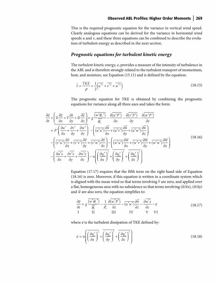
Observed ABL Profiles: Higher Order Moments 269
This is the required prognostic equation for the variance in vertical wind speed.
Clearly analogous equations can be derived for the variance in horizontal wind
speeds u and v, and these three equations can be combined to describe the evolu-
tion of turbulent energy as described in the next section.
Prognostic equations for turbulent kinetic energy
The turbulent kinetic energy, e, provides a measure of the intensity of turbulence in
the ABL and is therefore strongly related to the turbulent transport of momentum,
heat, and moisture, see Equation (15.11) and is defined by the equation:
( )′ ′ ′= = + +2 2 21
2
TKEe u v wr
(18.15)
The prognostic equation for TKE is obtained by combining the prognostic
equations for variance along all three axes and takes the form:
⎛ ⎞ ′ ′∂ ∂ ∂ ∂ ∂ ′ ′ ∂ ′ ′ ∂ ′ ′+ + + = − − −⎜ ⎟∂ ∂ ∂ ∂ ∂ ∂ ∂⎝ ⎠
⎛ ⎞⎛ ⎞∂ ′ ∂ ′ ∂ ′ ∂ ∂ ∂+ ′ + + − ′ ′ + ′ ′ + ′ ′⎜ ⎟⎜ ⎟∂ ∂ ∂ ∂ ∂ ∂⎝ ⎠ ⎝ ⎠
⎛ ⎞∂ ∂ ∂ ∂ ∂− ′ ′ + ′ ′ + ′ ′ − ′ ′ + ′ ′ + ′⎜ ⎟∂ ∂ ∂ ∂ ∂⎝ ⎠
( ) ( ) ( ) ( )
( ) ( ) ( )
( ) ( ) ( ) ( ) ( ) (
v
v
w u P v P w Pee e eu v w gt x y z x y z
u u uu v wP u u u v u wx y z x y z
w wv v vv u v v v w w u w v wx y z x y
⎛ ⎞∂′⎜ ⎟∂⎝ ⎠
⎛ ⎞⎛ ⎞ ⎛ ⎞∂ ′ ∂ ′ ∂ ′ ∂ ′ ∂ ′ ∂ ′⎛ ⎞ ⎛ ⎞⎜ ⎟− + + − υ + +⎜ ⎟ ⎜ ⎟⎜ ⎟ ⎜ ⎟⎝ ⎠ ⎝ ⎠∂ ∂ ∂ ∂ ∂ ∂⎝ ⎠⎜ ⎟⎝ ⎠ ⎝ ⎠
22 2
)wwz
u e v e w e u u ux y z x y z
(18.16)
Equation (17.17) requires that the fifth term on the right hand side of Equation
(18.16) is zero. Moreover, if this equation is written in a coordinate system which
is aligned with the mean wind so that terms involving v− are zero, and applied over
a flat, homogeneous area with no subsidence so that terms involving (∂/∂x), (∂/∂y)
and w− are also zero, the equation simplifies to:
( ) 1 ( )( )
I II II I IV V VI
v
av
uw w P w ee g u wt z z z
′ ′ ′ ′ ′∂ ∂ ∂ ∂′ ′= − − − −∂ ∂ ∂ ∂
q erq
(18.17)
where e is the turbulent dissipation of TKE defined by:
⎛ ⎞⎛ ⎞∂ ′ ∂ ′ ∂ ′⎛ ⎞ ⎛ ⎞⎜ ⎟= + +⎜ ⎟ ⎜ ⎟⎜ ⎟⎝ ⎠ ⎝ ⎠∂ ∂ ∂⎝ ⎠⎜ ⎟⎝ ⎠
22 2u u ux y z
e u
(18.18)
Shuttleworth_c18.indd 269Shuttleworth_c18.indd 269 11/3/2011 6:53:50 PM11/3/2011 6:53:50 PM
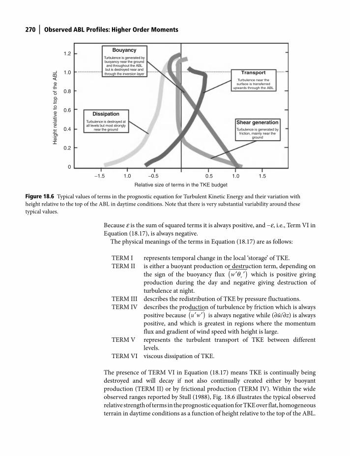
270 Observed ABL Profiles: Higher Order Moments
Because e is the sum of squared terms it is always positive, and −e, i.e., Term VI in
Equation (18.17), is always negative.
The physical meanings of the terms in Equation (18.17) are as follows:
TERM I represents temporal change in the local ‘storage’ of TKE.
TERM II is either a buoyant production or destruction term, depending on
the sign of the buoyancy flux ( )′ ′vw q which is positive giving
production during the day and negative giving destruction of
turbulence at night.
TERM III describes the redistribution of TKE by pressure fluctuations.
TERM IV describes the production of turbulence by friction which is always
positive because ( )′ ′u w is always negative while (∂ū/∂z) is always
positive, and which is greatest in regions where the momentum
flux and gradient of wind speed with height is large.
TERM V represents the turbulent transport of TKE between different
levels.
TERM VI viscous dissipation of TKE.
The presence of TERM VI in Equation (18.17) means TKE is continually being
destroyed and will decay if not also continually created either by buoyant
production (TERM II) or by frictional production (TERM IV). Within the wide
observed ranges reported by Stull (1988), Fig. 18.6 illustrates the typical observed
relative strength of terms in the prognostic equation for TKE over flat, homogeneous
terrain in daytime conditions as a function of height relative to the top of the ABL.
−1.5
0
0.2
0.4
0.6
0.8
1.0
1.2Bouyancy
Turbulence is generated bybuoyancy near the groundand throughout the ABL
but is destroyed near andthrough the inversion layer
DissipationTurbulence is destroyed atall levels but most strongly
near the ground
Shear generationTurbulence is generated by
friction, mainly near theground
TransportTurbulence near thesurface is transferred
upwards through the ABL
1.0 −0.5
Relative size of terms in the TKE budget
Hei
ght r
elat
ive
to to
p of
the
AB
L
0.5 1.0 1.5
Figure 18.6 Typical values of terms in the prognostic equation for Turbulent Kinetic Energy and their variation with
height relative to the top of the ABL in daytime conditions. Note that there is very substantial variability around these
typical values.
Shuttleworth_c18.indd 270Shuttleworth_c18.indd 270 11/3/2011 6:53:54 PM11/3/2011 6:53:54 PM
Observed ABL Profiles: Higher Order Moments 271
Figure 18.7 shows how TKE of air in the ABL is ‘spun up’ during the day and then
subsequently decays at night.
The turbulent kinetic energy in the ABL is present across a range of frequencies
and the shape of this spectrum evolves with time depending on local ambient
conditions. Figure 18.8a shows a typical spectrum for TKE in unstable conditions.
The terms in Equation (18.17) also have different spectra, and Fig. 18.8b shows the
spectra for the buoyant and shear production terms and the turbulent dissipation
term. This figure reveals that turbulence is largely produced at low frequency but
is mainly dissipated at high frequency. The energy present in large eddies provides
energy to smaller and smaller eddies until the secondary eddies so created are
small and the spatial gradients of variance in the viscous dissipation term, e, there-
fore large. The kinetic energy associated with motion in the turbulent air is then
dissipated through friction as heat.
Prognostic equations for variance of moisture and heat
The prognostic equation for the variance in the moisture content and heat
content of air in the ABL can be derived following procedures broadly analo-
gous to that used to derive Equation (18.13), the prognostic equations for the
0
0.5
0.761.18
0.40
0.30
0.18
0.05
1.05
0.93
0.68
0.430.30
0.18
0.05
0.68
0.55
0.43
0.300.18
0.05
Hei
ght (
km)
1.0
1.5
12
Day 1 Day 2
Time (hours)
Day 3
18 0 6 12 18 0 6
Figure 18.7 Measured TKE with height in daytime conditions at Wangara, Australia. (Redrawn from Yamada and Mellor,
1975, published with permission).
Shuttleworth_c18.indd 271Shuttleworth_c18.indd 271 11/3/2011 6:53:56 PM11/3/2011 6:53:56 PM

272 Observed ABL Profiles: Higher Order Moments
0.001
−0.4
−0.2
0.2
0.4
0
0.5
0
1.0(a)
(b)
0.01 0.1 1 10 100 1000
0.001 0.01 0.1 1 10 100 1000
TKE dissipated smalleddies by friction
TKE in large eddies producedby both buoyancy and shear
Rel
ativ
e si
ze o
fT
KE
term
sR
elat
ive
cont
ribut
ion
to T
KE
Energy transfer betweeneddy frequencies Dissipation
Shearproduction
Buoyantproduction
Frequency of turbulent eddy
Figure 18.8 (a) Typical example of the relative strength of the contributions to TKE at different frequencies; (b) typical
change in the relative magnitude of the production and destruction terms in the prognostic equation for TKE and the
energy transfer (between frequencies) as a function of eddy frequency.
variance in vertical wind speed. For moisture fluctuations the resulting equation
has the form:
( )2 2 2 2( ) ( ) ( )2
I II III
q q qq q q q + u. + v. + w. = q u . + q v . + q w .t x y z x y z
⎡ ⎤ ⎡ ⎤′ ′ ′ ′− ′ ′ ′ ′ ′ ′⎢ ⎥ ⎢ ⎥
⎢ ⎥⎢ ⎥ ⎣ ⎦⎣ ⎦
∂ ∂ ∂ ∂ ∂ ∂ ∂∂ ∂ ∂ ∂ ∂ ∂ ∂
22 22 2 2( ) ( ) ( )2
IV V
u q v q w q q q q + x y z x y z
⎡ ⎤⎡ ⎤ ⎛ ⎞′ ′ ′ ′ ′ ′ ′ ′ ′⎛ ⎞ ⎛ ⎞⎢ ⎥− + − + +⎢ ⎥ ⎜ ⎟ ⎜ ⎟⎜ ⎟⎝ ⎠ ⎝ ⎠⎢ ⎥⎝ ⎠⎢ ⎥⎣ ⎦ ⎣ ⎦
∂ ∂ ∂ ∂ ∂ ∂ν∂ ∂ ∂ ∂ ∂ ∂
(18.19)
Shuttleworth_c18.indd 272Shuttleworth_c18.indd 272 11/3/2011 6:53:57 PM11/3/2011 6:53:57 PM
Observed ABL Profiles: Higher Order Moments 273
The physical meanings of the terms in Equation (18.19) are as follows:
TERM I represents temporal change in the local ‘storage’ of moisture
variance.
TERM II describes the advection of moisture variance.
TERM III describes the production/consumption of moisture variance.
TERM IV represents the turbulent transport of moisture variance.
TERM V viscous dissipation of moisture variance by molecular processes.
Within the wide observed ranges reported by Stull (1988), Fig. 18.9a shows the
typical relative strength over flat, homogeneous terrain in daytime conditions of
moisture variance, and Fig. 18.9b the typical relative strength of the terms in
Equation (18.19), both as a function of height relative to the top of the ABL. The
production term is positive and the dissipation term negative throughout the
ABL, and both are greatest near the inversion layer. The turbulent transport term
describes the movement of moisture variance vertically within the ABL.
The prognostic equation for variance in potential temperature has the form:
⎡ ⎤ ⎡ ⎤′ ′ ′ ′+ + + = − ′ ′ + ′ ′ + ′ ′⎢ ⎥ ⎢ ⎥
⎢ ⎥ ⎣ ⎦⎣ ⎦
′( ′)− +
2 2 2 2
2
( ) ( ) ( ) ( ). . . 2 . . .
I I I III
u v w u v wt x y z x y z
u v x
∂ ∂ ∂ ∂ ∂ ∂ ∂∂ ∂ ∂ ∂ ∂ ∂ ∂
∂ ∂∂
q q q q q q qq q q
q ⎡ ⎤⎡ ⎤ ⎛ ⎞′( ′) ′( ′) ′ ′ ′⎛ ⎞ ⎛ ⎞⎢ ⎥+ − + +⎢ ⎥ ⎜ ⎟ ⎜ ⎟⎜ ⎟⎝ ⎠ ⎝ ⎠⎢ ⎥⎝ ⎠⎢ ⎥⎣ ⎦ ⎣ ⎦
⎛ ⎞− ′ + ′⎜ ⎟
⎝ ⎠
22 22 2
2
I V V
2
xn
a p
wy z x y z
Rc x
∂ ∂ ∂ ∂∂ ∂ ∂ ∂ ∂
∂ ∂∂
qq q q q q
u
q qr
⎡ ⎤+ ′⎢ ⎥
⎣ ⎦ VI
y zn nR R
y z∂
∂ ∂q
(18.20)
The physical meanings of the terms in Equation (18.20) are as follows:
TERM I represents temporal change in the local ‘storage’ of temperature
variance.
TERM II describes the advection of temperature variance.
TERM III describes the production/consumption of temperature variance.
TERM IV represents the turbulent transport of temperature variance.
TERM V viscous dissipation of temperature variance by molecular
processes.
TERM VI describes the destruction of temperature variance by gradients in
radiation.
Within the wide observed ranges reported by Stull (1988), Fig. 18.10a shows the
typical relative strength over flat, homogeneous terrain in daytime conditions of
Shuttleworth_c18.indd 273Shuttleworth_c18.indd 273 11/3/2011 6:53:58 PM11/3/2011 6:53:58 PM
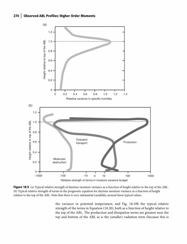
274 Observed ABL Profiles: Higher Order Moments
0
0
0.2 0.4 0.6 0.8 1.0 1.2
0.2
0.4
0.6
0.8
1.0
1.2
1.4
(a)
Relative variance in specific humidity
Hei
ght r
elat
ive
to to
p of
the
AB
L
−1000 −100 −10 0
Moleculardestruction
Turbulenttransport Production
(b)
10 100 1000
Relative strength of terms in moisture variance budget
0
0.2
0.4
0.6
0.8
1.0
1.2
Hei
ght r
elat
ive
to to
p of
the
AB
L
Figure 18.9 (a) Typical relative strength of daytime moisture variance as a function of height relative to the top of the ABL.
(b) Typical relative strength of terms in the prognostic equation for daytime moisture variance as a function of height
relative to the top of the ABL. Note that there is very substantial variability around these typical values.
the variance in potential temperature, and Fig. 18.10b the typical relative
strength of the terms in Equation (18.20), both as a function of height relative to
the top of the ABL. The production and dissipation terms are greatest near the
top and bottom of the ABL as is the (smaller) radiation term (because this is
Shuttleworth_c18.indd 274Shuttleworth_c18.indd 274 11/3/2011 6:53:59 PM11/3/2011 6:53:59 PM
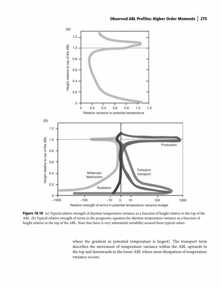
Observed ABL Profiles: Higher Order Moments 275
00
0.2 0.4 0.6 0.8 1.0 1.2
0.2
0.4
0.6
0.8
1.0
1.2
−1000 −100 −10 0
Moleculardestruction
Turbulenttransport
Radiation
Production
(b)
(a)
10 100 1000
Relative variance in potential temperature
Relative strength of terms in potential temperature variance budget
Hei
ght r
elat
ive
to to
p of
the
AB
L
0
0.2
0.4
0.6
0.8
1.0
1.2
Hei
ght r
elat
ive
to to
p of
the
AB
L
Figure 18.10 (a) Typical relative strength of daytime temperature variance as a function of height relative to the top of the
ABL. (b) Typical relative strength of terms in the prognostic equation for daytime temperature variance as a function of
height relative to the top of the ABL. Note that there is very substantial variability around these typical values.
where the gradient in potential temperature is largest). The transport term
describes the movement of temperature variance within the ABL upwards to
the top and downwards to the lower ABL where most dissipation of temperature
variance occurs.
Shuttleworth_c18.indd 275Shuttleworth_c18.indd 275 11/3/2011 6:54:00 PM11/3/2011 6:54:00 PM
276 Observed ABL Profiles: Higher Order Moments
Important points in this chapter
● ABL structure: during the day the lower atmosphere has four main layers:
(a) surface layer (∼100 m), strongly influenced by the surface; (b) mixed layer
(∼ 0.5–3 km), strongly turbulent; (c) entrainment layer (∼10–100 m), a thermal
inversion which inhibits mixing; and (d) free atmosphere (several km), with
limited turbulence.
● ABL growth: warmer drier air is ‘entrained’ downward into the mixed layer
through the inversion from the free atmosphere above so the ABL grows
during the day. At night the surface cools and a stable surface layer develops
which grows upward and is a partial barrier between the ground and residual
mixed layer.
● Daytime ABL properties: the growing daytime mixed layer is heated both by
sensible heat from the surface and by entrainment of warmer air from the
free atmosphere so ABL temperature increases, but vapor from the surface is
mainly used to moisten incoming drier entrained air so ABL humidity often
sees limited diurnal change.
● Nighttime ABL properties: the time evolution of mean variables is usually
more strongly dependent on atmospheric subsidence and longwave radia-
tion flux divergence at night than during the day.
● Evolution of variances: prognostic equations for turbulent departures
(e.g., u′, v′, w′, q′, q′) can be derived similar to those describing mean values
(e.g., u−, v−, w−, q−, q−), and these are used to derive prognostic equations for
variances, e.g., (u′)2, (v′)2, (w′)2, (q ′)2 and (q′)2.
● Evolution of TKE: the prognostic equations for velocity variances combine
to give the important prognostic equation for the turbulent kinetic energy
(TKE) with terms that describe the production, destruction, and transport
of TKE.
● Conservation of TKE: because TKE is continually being destroyed by
viscosity and created by buoyancy and friction at rates which vary with
atmospheric conditions, so is the capability to transport fluxes by turbulent
diffusion.
References
Carlson, M.A. and Stull, R.B. (1986) Subsidence in the nocturnal boundary layer. Journal
of Climate and Applied Meteorology, 25, 1088–1099.
Stull, R.B. (1988) An Introduction to Boundary Layer Meteorology (Atmospheric Sciences
Library). Kluger Academic Publishers, Dordrecht.
Yamada, T. and Mellor, G. (1975) Simulation of the Wangara atmospheric boundary layer
data. Journal of the Atmospheric Sciences, 32, 2309–2329.
Shuttleworth_c18.indd 276Shuttleworth_c18.indd 276 11/3/2011 6:54:00 PM11/3/2011 6:54:00 PM
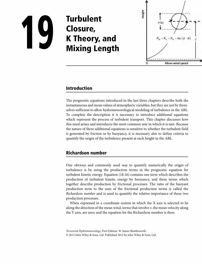
Introduction
The prognostic equations introduced in the last three chapters describe both the
instantaneous and mean values of atmospheric variables, but they are not by them-
selves sufficient to allow hydrometeorological modeling of turbulence in the ABL.
To complete the description it is necessary to introduce additional equations
which represent the process of turbulent transport. This chapter discusses how
this need arises and introduces the most common way in which it is met. Because
the nature of these additional equations is sensitive to whether the turbulent field
is generated by friction or by buoyancy, it is necessary also to define criteria to
quantify the origin of the turbulence present at each height in the ABL.
Richardson number
One obvious and commonly used way to quantify numerically the origin of
turbulence is by using the production terms in the prognostic equation for
turbulent kinetic energy. Equation (18.16) contains one term which describes the
production of turbulent kinetic energy by buoyancy, and three terms which
together describe production by frictional processes. The ratio of the buoyant
production term to the sum of the frictional production terms is called the
Richardson number and is used to quantify the relative importance of these two
production processes.
When expressed in a coordinate system in which the X axis is selected to lie
along the direction of the mean wind, terms that involve v, the mean velocity along
the Y axis, are zero, and the equation for the Richardson number is then:
19 Turbulent Closure, K Theory, and Mixing Length
Terrestrial Hydrometeorology, First Edition. W. James Shuttleworth.
© 2012 John Wiley & Sons, Ltd. Published 2012 by John Wiley & Sons, Ltd.
Shuttleworth_c19.indd 277Shuttleworth_c19.indd 277 11/3/2011 6:51:24 PM11/3/2011 6:51:24 PM
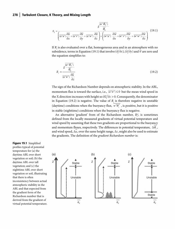
278 Turbulent Closure, K Theory, and Mixing Length
′ ′
′ ′ ′ ′ ′ ′ ′ ′ ′ ′ ′ ′
=
+ + + + +⎛ ⎞ ⎛ ⎞∂ ∂ ∂ ∂ ∂ ∂⎜ ⎟ ⎜ ⎟∂ ∂ ∂ ∂ ∂ ∂⎝ ⎠ ⎝ ⎠
( )
( ) ( ) ( ) ( ) ( ) ( )
v
vRi
wg
u u u w w wu u u v u w w u w v w wx y z x y z
qq (19.1)
If Ri is also evaluated over a flat, homogeneous area and in an atmosphere with no
subsidence, terms in Equation (19.1) that involve ( )x∂ ∂ , ( )y∂ ∂ and w are zero and
the equation simplifies to:
′ ′
′ ′
=∂∂
( )
( )
i
v
v
wgR
uu wz
(19.2)
The sign of the Richardson Number depends on atmospheric stability. In the ABL,
momentum flux is toward the surface, i.e., ( ) 0u w′ ′ ≤ but the mean wind speed in
the X direction increases with height so ∂ ∂ > 0u z . Consequently, the denominator
in Equation (19.2) is negative. The value of Ri is therefore negative in unstable
(daytime) conditions when the buoyancy flux, vw ′ ′q , is positive, but it is positive
in stable (nighttime) conditions when the buoyancy flux is negative.
An alternative ‘gradient’ from of the Richardson number, Rig, is sometimes
defined from the locally measured gradients of virtual potential temperature and
wind speed by assuming that these two gradients are proportional to the buoyancy
and momentum fluxes, respectively. The differences in potential temperature, vΔq ,
and wind speed, uΔ , over the same height range, zΔ , might also be used to estimate
the gradients. The definition of the gradient Richardson number is:
(a) (b) (c)
Z Z ZStable Stable Stable
Stable
UnstableUnstable
qv qv qv
Unstable
Figure 19.1 Simplified
profiles typical of potential
temperature for (a) the
daytime ABL over short
vegetation or soil; (b) the
daytime ABL over tall
vegetation; and (c) the
nighttime ABL over short
vegetation or soil, illustrating
that there is often
inconsistency between actual
atmospheric stability in the
ABL and that expected from
the gradient form of the
Richardson number that is
derived from the gradient of
virtual potential temperature.
Shuttleworth_c19.indd 278Shuttleworth_c19.indd 278 11/3/2011 6:51:25 PM11/3/2011 6:51:25 PM
Turbulent Closure, K Theory, and Mixing Length 279
( )⎡ ⎤⎛ ⎞ ⎛ ⎞ Δ∂ ∂⎢ ⎥= =⎜ ⎟ ⎜ ⎟∂ ∂⎢ ⎝ ⎠ ⎥⎝ ⎠ Δ⎣ ⎦
2
2org g vv
i iv v
g guR Rz z u
qqq q
(19.3)
Although often an acceptable estimate in the surface layer, where (as described later)
the turbulent fluxes are proportional to the gradient in mean values, the gradient
form of the Richardson number can be problematic when used elsewhere in the
ABL. This is shown in Fig. 19.1, which gives possible gradients of virtual potential
temperature and identifies the nature of the stability at different heights. The latter
are often inconsistent with the local gradient of virtual potential temperature.
Turbulent closure
Starting from the basic conservation equations for atmospheric flow, prognostic
equations were introduced in Chapter 17 that describe the evolution in space and
time of mean flow variables. These equations involved terms that include not only
mean flow variables but also turbulent fluxes, i.e., the time average of double cor-
relation coefficients. Then, in Chapter 18, prognostic equations were introduced
that describe the time average of turbulent variances in equations which involve
terms that include not only mean flow variables and turbulent fluxes, but also the
time averages of triple correlation coefficients. This process can be successively
repeated to derive prognostic equations for correlation coefficients of increasingly
higher complexity which contain terms that involved mean flow variables and cor-
relations of lower complexity. However, at each new level of complexity, the num-
ber of new unknown variables introduced into the prognostic equations derived
exceeds the number of equations available to describe them. Table 19.1 illustrates
Table 19.1 Progression of the sets of prognostic equations derived to describe
correlation coefficients of velocity with increasing complexity and the number
of new equations and new unknown combinations involved in these.
‘Moment’ or ‘order’
General form of equations
Number of new equations
New variables (and number of new variables)
Zero u , v , and w , are specified in space and time
0 u , v , w , (3)
First ( )∂ ′ ′∂ =∂ ∂
.......i ji
j
u uut x
3 ′2u , 2v ′ , 2w ′ , u v¢ ¢ , u w¢ ¢ , u w¢ ¢ , (6)
Second ( ).......
i j ki j
j
u u uu ut x
∂∂=
∂ ∂¢ ¢ ¢¢ ¢ 6 3u¢ , 3v¢ , 3w¢ , 2u v¢ ¢ , 2u w¢ ¢ , 2v u¢ ¢ ,
2v w¢ ¢ , 2w u¢ ¢ , 2w v¢ ¢ , u v w¢ ¢ ¢ , (10)
etc. etc. etc. etc.
Shuttleworth_c19.indd 279Shuttleworth_c19.indd 279 11/3/2011 6:51:35 PM11/3/2011 6:51:35 PM
280 Turbulent Closure, K Theory, and Mixing Length
the derivation of prognostic equations of escalating complexity for the case of
velocity components.
Because the process of deriving successive ‘orders’ of prognostic equations
always results in more new unknowns than new equations, it is not possible to use
this approach to derive a suite of physically based equations that by themselves are
an independent basis for describing turbulent transport in the ABL. To allow such
a description it is always necessary to provide additional equations that relate the
unknown variables to each order. The process of providing these additional
equations to complement the prognostic equations derived at any specific order of
complexity is known as making ‘turbulent closure’.
To obtain turbulent closure at a particular order it is necessary to ‘parameterize’
higher order moments in terms of lower order moments through new equations.
In practice, these additional equations are often observation-stimulated, and are
usually approximate descriptions that are applicable in restricted regions of the
ABL and/or in particular stability conditions. The range of turbulent closure
schemes that can be proposed is limited only by human ingenuity, but a closure
scheme is only credible if its use can be shown to result in a description that is
confirmed by observations. Proposed turbulent closure schemes can be local if the
values of unknown quantities at a specific point are assumed related to each other.
Or they can be nonlocal if some unknown quantities are related to other quantities
at many points. In this text the closure scheme described is that most commonly
used in the surface layer of the ABL, i.e., local closure at first order. However the
next section first discuses closure at lower order than this.
Low order closure schemes
The lowest order closure possible is zero order closure. This is the trivial case in
which the spatial and temporal distributions of mean atmospheric variables are
specified simply as numerical or algebraic functions, i.e., as global, regional, or
local space-time maps.
Sometimes a form of closure is used in the ABL in which the variation in space
and time of mean meteorological variables is described, but without explicit
representation of turbulent transport mechanisms. This approach is sometimes
called a Slab Model and is used to describe the daytime evolution of the ABL over
homogeneous, flat surfaces. In such a model the temperature and humidity profiles
are assumed to have a fixed (but plausible) height dependency, but the mean value
of these profiles changes with time in response to the input of sensible heat and
water vapor.
A slab model is illustrated in Fig. 19.2. The surface fluxes and rate of entrainment
into the ABL are described by subsidiary equations, and the divergence of fluxes is
assumed negative and constant with height. This is consistent with assuming the
two profiles have time-independent height dependence. The rates of change of
temperature and humidity content in the ‘slab’ are then calculated from
Shuttleworth_c19.indd 280Shuttleworth_c19.indd 280 11/3/2011 6:51:59 PM11/3/2011 6:51:59 PM
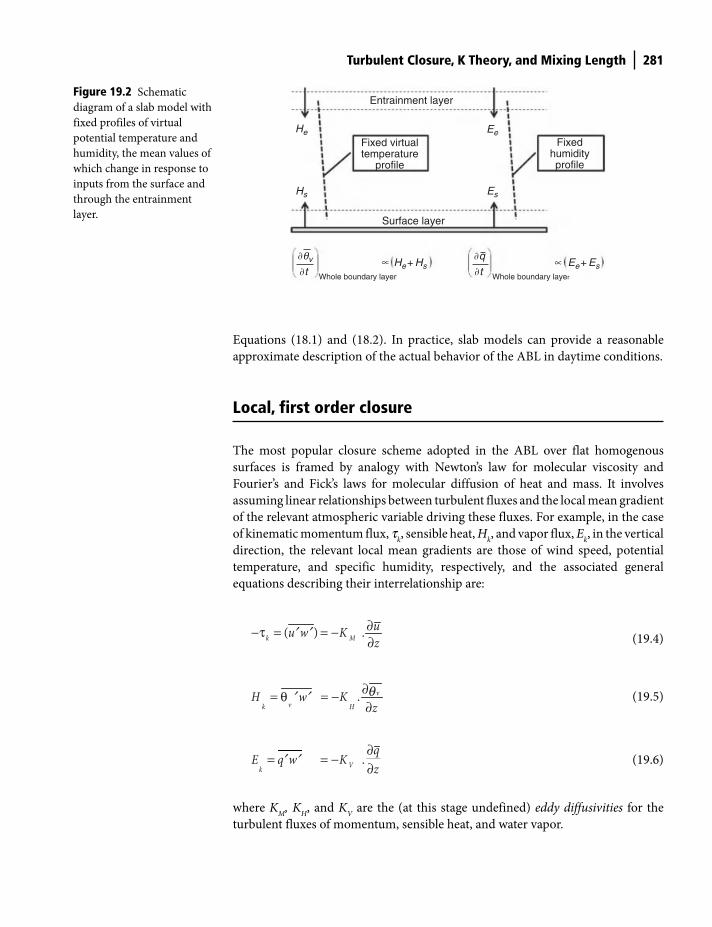
Turbulent Closure, K Theory, and Mixing Length 281
Equations (18.1) and (18.2). In practice, slab models can provide a reasonable
approximate description of the actual behavior of the ABL in daytime conditions.
Local, first order closure
The most popular closure scheme adopted in the ABL over flat homogenous
surfaces is framed by analogy with Newton’s law for molecular viscosity and
Fourier’s and Fick’s laws for molecular diffusion of heat and mass. It involves
assuming linear relationships between turbulent fluxes and the local mean gradient
of the relevant atmospheric variable driving these fluxes. For example, in the case
of kinematic momentum flux, tk, sensible heat, H
k, and vapor flux, E
k, in the vertical
direction, the relevant local mean gradients are those of wind speed, potential
temperature, and specific humidity, respectively, and the associated general
equations describing their interrelationship are:
∂−τ = = −∂
( ) .k Muu w Kz
¢ ¢ (19.4)
∂= = −θ∂
.vk H
vH Kwz
q¢ ¢ (19.5)
∂= = −
∂.
k V
qE q w K
z¢ ¢ (19.6)
where KM
, KH, and K
V are the (at this stage undefined) eddy diffusivities for the
turbulent fluxes of momentum, sensible heat, and water vapor.
Figure 19.2 Schematic
diagram of a slab model with
fixed profiles of virtual
potential temperature and
humidity, the mean values of
which change in response to
inputs from the surface and
through the entrainment
layer.
Fixed virtualtemperature
profile
Fixedhumidityprofile
Entrainment layer
Surface layer
Whole boundary layer
�qv
�t
�q
�t Whole boundary layer
He
Hs
He+ Hs Ee+ Es
Es
Ee
∝ ∝
Shuttleworth_c19.indd 281Shuttleworth_c19.indd 281 11/3/2011 6:51:59 PM11/3/2011 6:51:59 PM
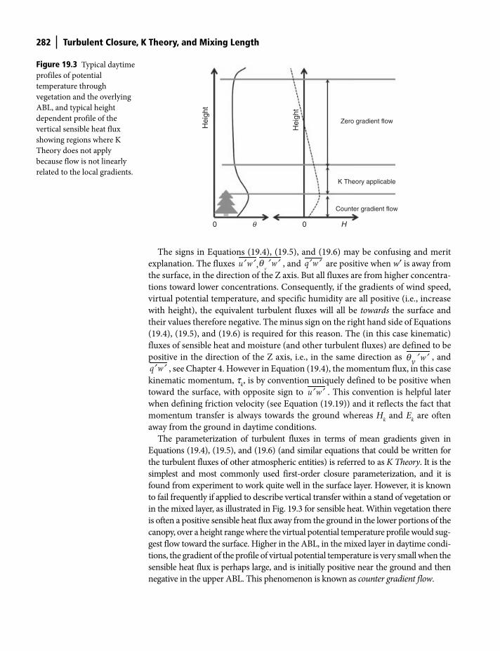
282 Turbulent Closure, K Theory, and Mixing Length
The signs in Equations (19.4), (19.5), and (19.6) may be confusing and merit
explanation. The fluxes , vwu w q ¢ ¢¢ ¢ , and q w¢ ¢ are positive when w′ is away from
the surface, in the direction of the Z axis. But all fluxes are from higher concentra-
tions toward lower concentrations. Consequently, if the gradients of wind speed,
virtual potential temperature, and specific humidity are all positive (i.e., increase
with height), the equivalent turbulent fluxes will all be towards the surface and
their values therefore negative. The minus sign on the right hand side of Equations
(19.4), (19.5), and (19.6) is required for this reason. The (in this case kinematic)
fluxes of sensible heat and moisture (and other turbulent fluxes) are defined to be
positive in the direction of the Z axis, i.e., in the same direction as wvq ¢ ¢ , and
q w¢ ¢ , see Chapter 4. However in Equation (19.4), the momentum flux, in this case
kinematic momentum, tk, is by convention uniquely defined to be positive when
toward the surface, with opposite sign to u w¢ ¢ . This convention is helpful later
when defining friction velocity (see Equation (19.19)) and it reflects the fact that
momentum transfer is always towards the ground whereas Hk and E
k are often
away from the ground in daytime conditions.
The parameterization of turbulent fluxes in terms of mean gradients given in
Equations (19.4), (19.5), and (19.6) (and similar equations that could be written for
the turbulent fluxes of other atmospheric entities) is referred to as K Theory. It is the
simplest and most commonly used first-order closure parameterization, and it is
found from experiment to work quite well in the surface layer. However, it is known
to fail frequently if applied to describe vertical transfer within a stand of vegetation or
in the mixed layer, as illustrated in Fig. 19.3 for sensible heat. Within vegetation there
is often a positive sensible heat flux away from the ground in the lower portions of the
canopy, over a height range where the virtual potential temperature profile would sug-
gest flow toward the surface. Higher in the ABL, in the mixed layer in daytime condi-
tions, the gradient of the profile of virtual potential temperature is very small when the
sensible heat flux is perhaps large, and is initially positive near the ground and then
negative in the upper ABL. This phenomenon is known as counter gradient flow.
Hei
ght
Hei
ght
Zero gradient flow
Counter gradient flow
K Theory applicable
0 q 0 H
Figure 19.3 Typical daytime
profiles of potential
temperature through
vegetation and the overlying
ABL, and typical height
dependent profile of the
vertical sensible heat flux
showing regions where K
Theory does not apply
because flow is not linearly
related to the local gradients.
Shuttleworth_c19.indd 282Shuttleworth_c19.indd 282 11/3/2011 6:52:03 PM11/3/2011 6:52:03 PM
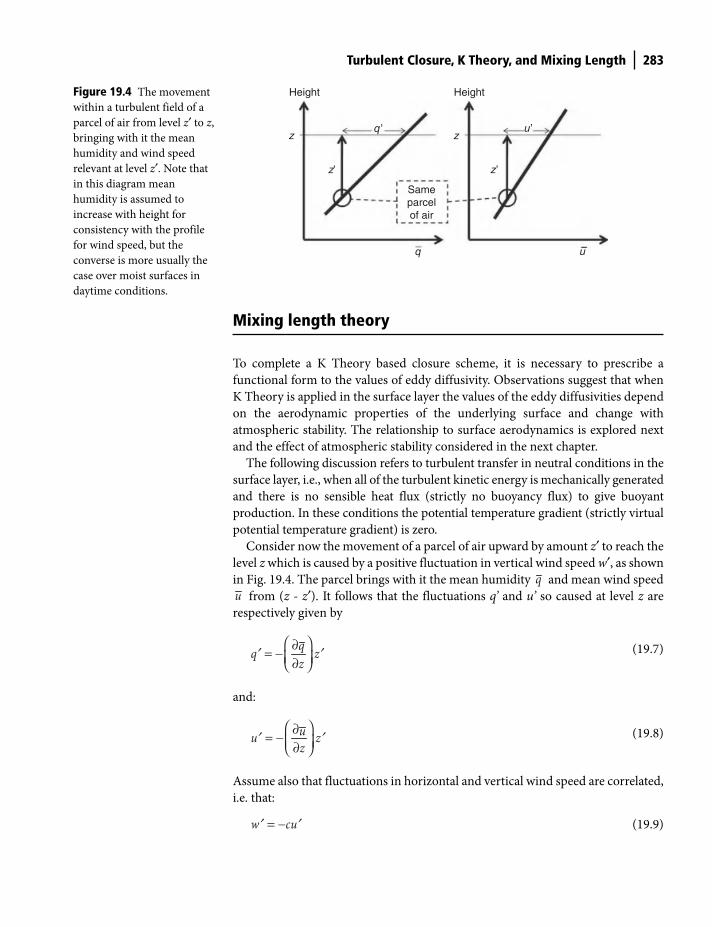
Turbulent Closure, K Theory, and Mixing Length 283
Mixing length theory
To complete a K Theory based closure scheme, it is necessary to prescribe a
functional form to the values of eddy diffusivity. Observations suggest that when
K Theory is applied in the surface layer the values of the eddy diffusivities depend
on the aerodynamic properties of the underlying surface and change with
atmospheric stability. The relationship to surface aerodynamics is explored next
and the effect of atmospheric stability considered in the next chapter.
The following discussion refers to turbulent transfer in neutral conditions in the
surface layer, i.e., when all of the turbulent kinetic energy is mechanically generated
and there is no sensible heat flux (strictly no buoyancy flux) to give buoyant
production. In these conditions the potential temperature gradient (strictly virtual
potential temperature gradient) is zero.
Consider now the movement of a parcel of air upward by amount z′ to reach the
level z which is caused by a positive fluctuation in vertical wind speed w′, as shown
in Fig. 19.4. The parcel brings with it the mean humidity q and mean wind speed
u from (z - z′). It follows that the fluctuations q’ and u’ so caused at level z are
respectively given by
qq zz
⎛ ⎞∂= −⎜ ⎟∂⎝ ⎠¢ ¢
(19.7)
and:
uu zz
⎛ ⎞∂= −⎜ ⎟∂⎝ ⎠¢ ¢
(19.8)
Assume also that fluctuations in horizontal and vertical wind speed are correlated,
i.e. that:
w cu= −¢ ¢ (19.9)
z
Height Height
Sameparcelof air
z ’ z ’
q ’ u ’
q u
z
Figure 19.4 The movement
within a turbulent field of a
parcel of air from level z′ to z,
bringing with it the mean
humidity and wind speed
relevant at level z′. Note that
in this diagram mean
humidity is assumed to
increase with height for
consistency with the profile
for wind speed, but the
converse is more usually the
case over moist surfaces in
daytime conditions.
Shuttleworth_c19.indd 283Shuttleworth_c19.indd 283 11/3/2011 6:52:07 PM11/3/2011 6:52:07 PM
284 Turbulent Closure, K Theory, and Mixing Length
Note that the minus sign appears in Equation (19.9) because the fluctuation w′, which is positive away from the surface, results in a fluctuation in horizontal wind
speed at the level z which is negative relative to the mean wind speed at that level.
The turbulent kinematic flux of water vapor is by definition the time average
value of the product of fluctuations in specific humidity and vertical wind speed,
and it can be obtained by substituting for q′ from Equation (19.7) and w′ from
(19.9) and averaging, i.e.
. . .q uq w z c zz z
⎧ ⎫⎧ ⎫ ⎡ ⎤⎛ ⎞ ⎛ ⎞∂ ∂⎪ ⎪⎪ ⎪= − − −⎢ ⎥⎨ ⎬⎨ ⎬⎜ ⎟ ⎜ ⎟∂ ∂⎝ ⎠ ⎝ ⎠⎢ ⎥⎪ ⎪⎪ ⎪⎩ ⎭ ⎣ ⎦⎩ ⎭¢ ¢ ¢ ¢
(19.10)
which simplifies to:
2. .( ) . q uq w c zz z
⎛ ⎞ ⎛ ⎞∂ ∂= − ⎜ ⎟ ⎜ ⎟∂ ∂⎝ ⎠ ⎝ ⎠¢ ¢ ¢
(19.11)
The basis of mixing length theory is the postulate that, providing turbulence is
solely frictional in origin, it can be characterized by a hypothetical mixing length,
l, whose value is assumed to represent the effective average vertical size of the
turbulent eddies in the turbulent field that transports atmospheric entities. In the
surface layer of the ABL the mixing length is defined such as to simplify
Equation (19.11) by:
2 2.( )c z=l ¢ (19.12)
and Equation (19.11) becomes:
2. . q uq wz z
⎛ ⎞ ⎛ ⎞∂ ∂= − ⎜ ⎟ ⎜ ⎟∂ ∂⎝ ⎠ ⎝ ⎠l¢ ¢
(19.13)
In a similar way, it can be shown that the momentum flux is given by:
2 . u uu wz z
⎛ ⎞ ⎛ ⎞∂ ∂= − ⎜ ⎟ ⎜ ⎟∂ ∂⎝ ⎠ ⎝ ⎠l¢ ¢
(19.14)
By comparing Equation (19.13) with Equation (19.6) and Equation (19.14) with
Equation (19.4) it follows that:
2 .M VuK Kz
⎛ ⎞∂= = ⎜ ⎟∂⎝ ⎠l
(19.15)
But it still remains necessary to assign a value to the mixing length, l.
Shuttleworth_c19.indd 284Shuttleworth_c19.indd 284 11/3/2011 6:52:13 PM11/3/2011 6:52:13 PM
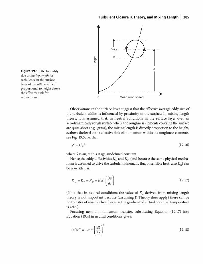
Turbulent Closure, K Theory, and Mixing Length 285
Observations in the surface layer suggest that the effective average eddy size of
the turbulent eddies is influenced by proximity to the surface. In mixing length
theory, it is assumed that, in neutral conditions in the surface layer over an
aerodynamically rough surface where the roughness elements covering the surface
are quite short (e.g., grass), the mixing length is directly proportion to the height,
z, above the level of the effective sink of momentum within the roughness elements,
see Fig. 19.5, i.e. that:
2 2 2k z=l (19.16)
where k is an, at this stage, undefined constant.
Hence the eddy diffusivities KM
and KV, (and because the same physical mecha-
nism is assumed to drive the turbulent kinematic flux of sensible heat, also KH) can
be re-written as:
2 2 .M V HuK K K k zz
⎛ ⎞∂= = = ⎜ ⎟∂⎝ ⎠
(19.17)
(Note that in neutral conditions the value of KH derived from mixing length
theory is not important because (assuming K Theory does apply) there can be
no transfer of sensible heat because the gradient of virtual potential temperature
is zero.)
Focusing next on momentum transfer, substituting Equation (19.17) into
Equation (19.4) in neutral conditions gives:
( )2
2 2 uu w k zz
⎛ ⎞∂= − ⎜ ⎟∂⎝ ⎠¢ ¢
(19.18)
Mean wind speedH
eigh
t
z
0
I = kz
Figure 19.5 Effective eddy
size or mixing length for
turbulence in the surface
layer of the ABL assumed
proportional to height above
the effective sink for
momentum.
Shuttleworth_c19.indd 285Shuttleworth_c19.indd 285 11/3/2011 6:52:18 PM11/3/2011 6:52:18 PM
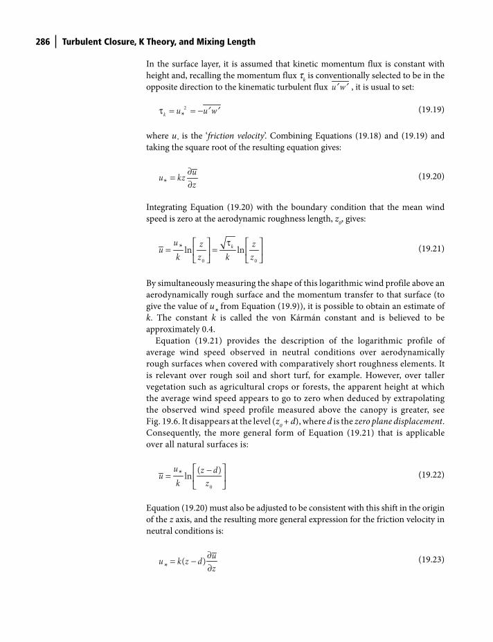
286 Turbulent Closure, K Theory, and Mixing Length
In the surface layer, it is assumed that kinetic momentum flux is constant with
height and, recalling the momentum flux tk is conventionally selected to be in the
opposite direction to the kinematic turbulent flux u w¢ ¢ , it is usual to set:
τ = = −2
*k u u w¢ ¢
(19.19)
where u* is the ‘friction velocity’. Combining Equations (19.18) and (19.19) and
taking the square root of the resulting equation gives:
∂=
∂*uu kzz
(19.20)
Integrating Equation (19.20) with the boundary condition that the mean wind
speed is zero at the aerodynamic roughness length, z0, gives:
τ⎡ ⎤ ⎡ ⎤= =⎢ ⎥ ⎢ ⎥
⎣ ⎦ ⎣ ⎦0 0
* ln lnku z zu
k z k z
(19.21)
By simultaneously measuring the shape of this logarithmic wind profile above an
aerodynamically rough surface and the momentum transfer to that surface (to
give the value of u* from Equation (19.9)), it is possible to obtain an estimate of
k. The constant k is called the von Kármán constant and is believed to be
approximately 0.4.
Equation (19.21) provides the description of the logarithmic profile of
average wind speed observed in neutral conditions over aerodynamically
rough surfaces when covered with comparatively short roughness elements. It
is relevant over rough soil and short turf, for example. However, over taller
vegetation such as agricultural crops or forests, the apparent height at which
the average wind speed appears to go to zero when deduced by extrapolating
the observed wind speed profile measured above the canopy is greater, see
Fig. 19.6. It disappears at the level (z0 + d), where d is the zero plane displacement.
Consequently, the more general form of Equation (19.21) that is applicable
over all natural surfaces is:
⎡ ⎤−= ⎢ ⎥
⎣ ⎦0
( )* lnu z duk z
(19.22)
Equation (19.20) must also be adjusted to be consistent with this shift in the origin
of the z axis, and the resulting more general expression for the friction velocity in
neutral conditions is:
∂= −
∂( )
*uu k z dz
(19.23)
Shuttleworth_c19.indd 286Shuttleworth_c19.indd 286 11/3/2011 6:52:21 PM11/3/2011 6:52:21 PM
Turbulent Closure, K Theory, and Mixing Length 287
while, on the basis of mixing length theory, the general expression for eddy
diffusion coefficients applicable in neutral conditions in the surface layer of the
ABL is:
= = = −( )*M V HK K K ku z d
(19.24)
The friction velocity u* may be substituted into Equation (19.24) from Equation
(19.21) to give:
2 1
0
( )( )lnM V H
z dK K K k u z dz
− ⎡ ⎤−= = = − ⎢ ⎥⎣ ⎦
(19.25)
or substituted from Equation (19.23) to give:
2 2( )M V HuK K K k z dz
∂= = = −∂
(19.26)
Thus, in conclusion, in neutral conditions in the surface layer, substituting the
value of eddy diffusivity from Equation (19.26) can be used in Equations (19.4),
(19.5), and (19.6) to give the required first order local turbulent closure equations:
∂−τ = − = = − −
∂2 ( )
* *kuu u w ku z dz
¢ ¢
(19.27)
⎛ ⎞∂= = − − ⎜ ⎟∂⎝ ⎠
( )*
vk vH w ku z d
zq
q ¢ ¢
(19.28)
4
3
2
1
0 00
2 2 31 13
Hei
ght (
m)
4
3
2
1
0
Hei
ght (
m)
Tall crop
d
Wind speed (m s−1) Wind speed (m s−1)
Short grass
Figure 19.6 Observed
profiles of average wind speed
over short grass and tall crops
demonstrating that the
position of zero wind speed
as deduced from
measurements above the crop
is elevated by the zero plane
displacement.
Shuttleworth_c19.indd 287Shuttleworth_c19.indd 287 11/3/2011 6:52:27 PM11/3/2011 6:52:27 PM
288 Turbulent Closure, K Theory, and Mixing Length
⎛ ⎞∂= = − − ⎜ ⎟∂⎝ ⎠
( )*k
qE q w ku z d
z¢ ¢
(19.29)
In the next chapter this first order local closure scheme is generalized to provide
equations that apply in other conditions of atmospheric stability.
Important points in this chapter
● Richardson number: is the ratio of the buoyancy to frictional production
terms in the prognostic equation for turbulent kinetic energy and is used to
quantify the origin of turbulence and atmospheric stability. When the X axis
is selected along the mean wind over a flat homogeneous area with no
subsistence, it is given by Equation (19.2).
● Gradient Richardson number: measured gradients of virtual potential
temperature and wind speed are used to estimate the Richardson Number
using Equation (19.3); this is risky because fluxes are not necessarily
proportional to gradients at all heights and in all conditions (Fig. 19.1).
● Turbulent closure: in principle it is possible to derive a succession of
prognostic equations that describe correlation coefficients in terms of mean
flow variables and correlations of lower complexity, but at each level of
complexity the number of unknown variables exceeds the number of
equations introduced to describe them. It is therefore necessary to provide
additional equations relating the unknown variables, and providing these is
known as making turbulent closure.
● K theory: is first order closure in which it is assumed kinematic fluxes (e.g.,
tk, H
k and E
k) are proportional to relevant local mean gradients (e.g., of wind
speed, potential temperature and specific humidity, respectively) with
proportionality constants (e.g., KM
, KH, and K
V, respectively) that are called
eddy diffusivities.
● Mixing length theory: assumes that in neutral conditions turbulence is
characterized by a hypothetical mixing length whose value is given by
multiplying the von Kármán constant (k ∼ 0.4) by the height above the ground
for short crops, or height above zero plane displacement for tall crops, giving
Equation (19.24).
Shuttleworth_c19.indd 288Shuttleworth_c19.indd 288 11/3/2011 6:52:32 PM11/3/2011 6:52:32 PM
Introduction
In the previous chapter, first order closure equations were defined by analogy with
molecular transfer processes. These equations related the kinematic turbulent
fluxes of momentum, sensible heat and latent heat to the mean profiles of wind
speed, virtual potential temperature and specific humidity through the (initially
unspecified) eddy diffusivities KM
, KH, and K
V, respectively. Observationally-
guided mixing length theory was then introduced to argue that in neutral
conditions KM
, KH, and K
V are all equal and can be expressed in terms of the von
Kármán constant, the height above the zero plane displacement, and either u* as in
Equation (19.23) or the mean wind speed and aerodynamic roughness length as
in Equation (19.24).
Here, we go further than this and seek first order closure in unstable and stable
conditions. Providing the aerodynamics of the surface exchange is expressed in
dimensionless form, the influence of stability can be accounted for using
hypothetically universal, empirical correction functions. Such functions, which
are often called stability corrections, are necessarily also parameterized in terms
of an appropriately defined dimensionless measure of atmospheric stability.
The mathematical procedure used to define this dimensionless representation of
aerodynamic transfer and dimensionless stability corrections is called surface
layer scaling.
Once first order closure based on mixing length theory has been generalized
to apply in all stability conditions, the resulting equations can be re-expressed in
an alternative form that considers the rates of surface exchange by turbulent
transfer as being controlled by a resistance to flow called aerodynamic resistance.
The representation of inhibition to surface transfers in terms of resistances is now
widely accepted and almost universally adopted in models.
20 Surface Layer Scaling and Aerodynamic Resistance
Terrestrial Hydrometeorology, First Edition. W. James Shuttleworth.
© 2012 John Wiley & Sons, Ltd. Published 2012 by John Wiley & Sons, Ltd.
Shuttleworth_c20.indd 289Shuttleworth_c20.indd 289 11/3/2011 6:49:49 PM11/3/2011 6:49:49 PM
290 Surface Layer Scaling and Aerodynamic Resistance
Dimensionless gradients
The theory of surface layer scaling is assumed to apply in the surface layer of the
ABL where it is also assumed that all vertical fluxes (of momentum, sensible heat
and water vapor, for example) are constant with height. The theory also applies
above uniform horizontal surfaces where there are no changes in the mean values
of atmospheric variables and fluxes of atmospheric entities in horizontal direc-
tions, and no subsidence. In these conditions, the prognostic equation for turbu-
lent kinetic energy is simplified to the form given earlier as Equation (18.17).
Remembering that because the momentum flux is assumed independent of
height in the surface layer, Equation (19.19) requires that u* is also independent of
height. Equation (18.17) can be re-written in dimensionless form by multiplying
by the factor [k(z-d)/(u*)3], as follows:
( )
′ ′ ∂ ′ ′− ∂ − −= −
∂ ∂
− ∂ − ∂ ′− ′ ′ − −
∂ ∂
3 3 3
3 3
( ) ( )( ) ( ) 1 ( )
( ) ( ) ( )* * *
I II III
( ) ( ) (
( ) ( )* *
v
v a
we w pk z d k z d k z dgt zu u u
k z d u k z d w e k zu wz zu u
qrq
−3
)
( )*
IV V VII
du
e
(20.1)
From the definition of u* in Equation (19.19), it follows that = −2 ( )
*u u w¢ ¢ and
term IV in Equation (20.1) can be simplified to:
*
( )M
uk z du z− ∂=
∂f
(20.2)
The function on the right hand side of Equation (20.2) is called the dimensionless
gradient of wind speed. When written in this dimensionless form, the wind speed
gradient in the surface layer has been normalized to allow for the local surface-
related dependency on u* and for height above the zero plane displacement. The
dimensionless function fM
on the left hand side of Equation (20.2) is as yet unspec-
ified, both in terms of functional form and purpose. However, multiplying
Equation (20.2) by (-u*
2/fM
) gives:
2 1
* *( ) ( )M
uu ku z dz
− ∂− = − −∂
f
(20.3)
Comparing this equation with Equation (19.27) suggests that the function fM
is
a dimensionless function whose reciprocal acts to change the effective average
vertical size (i.e. the mixing length) of the turbulent eddies operating in the
surface layer. In neutral stability conditions, comparison between Equations
(19.27) and (20.3) requires that fM
= 1, but in other conditions of thermal
Shuttleworth_c20.indd 290Shuttleworth_c20.indd 290 11/3/2011 6:49:50 PM11/3/2011 6:49:50 PM
Surface Layer Scaling and Aerodynamic Resistance 291
stability (as characterized by an as yet undefined dimensionless measure of
buoyant production) its value may change.
We return to this point later, but meanwhile next consider how it is possible
to define other dimensionless gradients of atmospheric entities, including fH
corresponding to kinematic sensible heat flux and virtual potential temperature,
and fV corresponding to kinematic moisture flux and specific humidity. Bearing
in mind the purpose these dimensionless functions serve (i.e., to modify the effec-
tive average mixing length of the turbulent eddies operating in the surface layer),
by analogy with Equation (20.3) it is possible to re-write Equation (19.28) in the
form:
−⎛ ⎞∂
= − − ⎜ ⎟∂⎝ ⎠1( ) ( )
*v
v Hw ku z dzq
q ¢ ¢ f
(20.4)
which can then be rearranged to define the dimensionless gradient of virtual
potential temperature thus:
∂−=
∂( )
*
vH
k z dzq
fq
(20.5)
where:
−=
( )*
*
v wu
q ¢ ¢q
(20.6)
Similarly Equation (19.29) can be re-written as:
− ⎛ ⎞∂= − − ⎜ ⎟∂⎝ ⎠
1( ) ( )* V
qq w ku z dz
¢ ¢ f
(20.7)
which can be rearranged to define the dimensionless gradient of specific
humidity:
∂−=
∂( )
*V
qk z dq z
f
(20.8)
where:
−=
( )*
*
q wqu¢ ¢
(20.9)
As is the case for the dimensionless wind speed gradient, when written in the
dimensionless form of Equations (20.5) and (20.8), respectively, the gradient of
Shuttleworth_c20.indd 291Shuttleworth_c20.indd 291 11/3/2011 6:49:50 PM11/3/2011 6:49:50 PM
292 Surface Layer Scaling and Aerodynamic Resistance
virtual potential temperature and gradient of specific humidity in the surface layer
are normalized to allow for the local surface-related dependency on u* and height
above the zero plane displacement.
At this stage, the mixing length hypothesis has been rewritten such that the
effective mixing length which controls turbulent transport in the surface layer
can be modified by the value of the dimensionless functions fM
, fH and f
V.
These functions are all equal to unity in neutral conditions, but their value may
alter with the extent of buoyant production or destruction in the turbulent
field. It is next necessary to assume that the functional forms of dimensionless
functions fM
, fH and f
V are a universal feature of turbulence in the surface layer
and independent of the actual surface itself. Although these dimensionless
functions are not known, if they are indeed universally applicable they can
presumably be defined by calculation from measured gradients and fluxes at
one place using Equations (20.2), (20.5) and (20.8), and the functional forms
so defined may then be applied everywhere. But the next step is to define a
dimensionless measure of the rate of buoyant production/destruction in
terms of which the empirical functional form of fM
, fH and f
V can be defined
by experiment.
Obukhov length
Equation (20.1), i.e., the dimensionless form of the prognostic equation for
turbulent kinetic energy, can be used to define the required dimensionless
measure of buoyant production/destruction in terms of which fM
, fH and f
V can
be parameterized. In this equation, Term II describes the contribution of buoyancy
to the production or destruction of turbulence. This term can be re-written in the
form (z-d)/L where L is called the Obukhov length and defined by:
−=
3( )*
( )
v
v
uL
gk w
q
q ¢ ¢
(20.10)
Because all the other factors on the right hand side of Equation (20.10) are positive,
the Obukhov length, and therefore (z-d)/L, takes its sign as being opposite to the
sign of the kinematic sensible heat flux, v wq ¢ ¢ . Consequently, L is negative when
the heat flux is positive (often in daytime conditions), and L is positive when the
heat flux is negative (often in nighttime conditions). One physical interpretation
of the Obukhov Length is that the value (-L) corresponds to the height at which
buoyant production of turbulent kinetic energy begins to dominate over shear
(mechanical) production when the mean profiles are assumed to be logarithmic
through the whole surface layer.
Not surprisingly, the factor (z-d)/L is formally related to the flux form of the
Richardson number, at least in neutral conditions, as can be shown by rearranging
terms in (z-d)/L as follows:
Shuttleworth_c20.indd 292Shuttleworth_c20.indd 292 11/3/2011 6:49:50 PM11/3/2011 6:49:50 PM
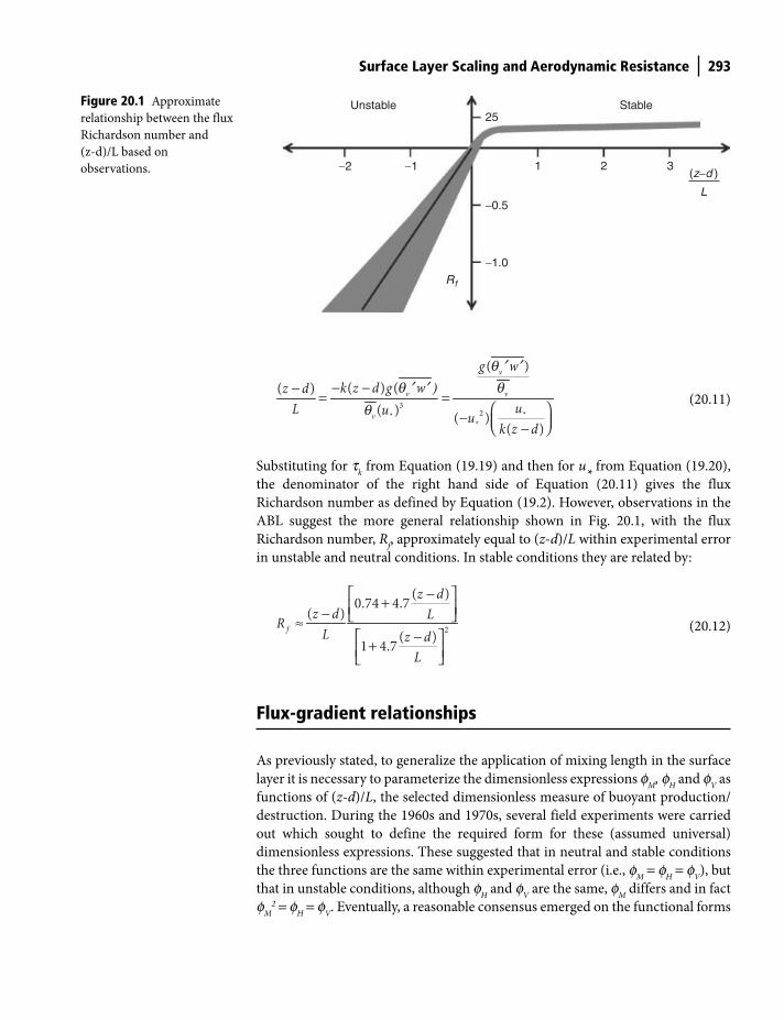
Surface Layer Scaling and Aerodynamic Resistance 293
32 **
*
( )
( ) (( )
( )( )
( )
v
v v
v
g wk z d g wz d
uL u uk z d
− −− = =⎛ ⎞− ⎜ ⎟⎝ ⎠−
q ¢ ¢q ¢ ¢ ) q
q
(20.11)
Substituting for tk from Equation (19.19) and then for u
* from Equation (19.20),
the denominator of the right hand side of Equation (20.11) gives the flux
Richardson number as defined by Equation (19.2). However, observations in the
ABL suggest the more general relationship shown in Fig. 20.1, with the flux
Richardson number, Rf, approximately equal to (z-d)/L within experimental error
in unstable and neutral conditions. In stable conditions they are related by:
2
( )0.74 4.7
( )
( )1 4.7
f
z dz d LRL z d
L
−⎡ ⎤+⎢ ⎥− ⎣ ⎦≈−⎡ ⎤+⎢ ⎥⎣ ⎦
(20.12)
Flux-gradient relationships
As previously stated, to generalize the application of mixing length in the surface
layer it is necessary to parameterize the dimensionless expressions fM
, fH and f
V as
functions of (z-d)/L, the selected dimensionless measure of buoyant production/
destruction. During the 1960s and 1970s, several field experiments were carried
out which sought to define the required form for these (assumed universal)
dimensionless expressions. These suggested that in neutral and stable conditions
the three functions are the same within experimental error (i.e., fM
= fH = f
V), but
that in unstable conditions, although fH and f
V are the same, f
M differs and in fact
fM
2 = fH = f
V. Eventually, a reasonable consensus emerged on the functional forms
−1.0
−0.5
25
1−1−2 2 3(z−d )
L
Unstable Stable
Rf
Figure 20.1 Approximate
relationship between the flux
Richardson number and
(z-d)/L based on
observations.
Shuttleworth_c20.indd 293Shuttleworth_c20.indd 293 11/3/2011 6:49:50 PM11/3/2011 6:49:50 PM
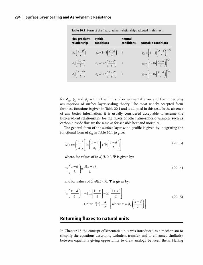
294 Surface Layer Scaling and Aerodynamic Resistance
for fM
, fH and f
V within the limits of experimental error and the underlying
assumptions of surface layer scaling theory. The most widely accepted form
for these functions is given in Table 20.1 and is adopted in this text. In the absence
of any better information, it is usually considered acceptable to assume the
flux- gradient relationships for the fluxes of other atmospheric variables such as
carbon dioxide flux are the same as for sensible heat and moisture.
The general form of the surface layer wind profile is given by integrating the
functional form of fM
in Table 20.1 to give:
⎡ ⎤⎛ ⎞− −⎛ ⎞ ⎛ ⎞= + Ψ⎢ ⎥⎜ ⎟⎜ ⎟ ⎜ ⎟ ⎝ ⎠⎝ ⎠ ⎝ ⎠⎢ ⎥⎣ ⎦*
0
( ) lnu z d z du zk z L
(20.13)
where, for values of (z-d)/L ≥ 0, Ψ is given by:
5( )z d z dL L− −⎛ ⎞Ψ =⎜ ⎟⎝ ⎠
(20.14)
and for values of (z-d)/L < 0, Ψ is given by:
π φ−
⎡ ⎤− + +⎛ ⎞ ⎡ ⎤Ψ = − − ⎢ ⎥⎜ ⎟ ⎢ ⎥⎝ ⎠ ⎣ ⎦ ⎣ ⎦⎡ ⎤−⎛ ⎞+ − ⎜ ⎟⎢ ⎥⎝ ⎠⎣ ⎦
2
1
1 12ln ln
2 2
2tan [ ] where x = 2
M
z d x xL
z dxL
(20.15)
Returning fluxes to natural units
In Chapter 15 the concept of kinematic units was introduced as a mechanism to
simplify the equations describing turbulent transfer, and to enhanced similarity
between equations giving opportunity to draw analogy between them. Having
Table 20.1 Form of the flux-gradient relationships adopted in this text.
Flux gradient relationship
Stable conditions
Neutral conditions Unstable conditions
φ −⎛ ⎞⎜ ⎟⎝ ⎠Mz dL
φ −⎛ ⎞= + ⎜ ⎟⎝ ⎠1 5Mz dL
1−
−⎡ ⎤⎛ ⎞= − ⎜ ⎟⎢ ⎥⎝ ⎠⎣ ⎦
14
1 16Mz dL
φ
φ −⎛ ⎞⎜ ⎟⎝ ⎠Hz dL
φ −⎛ ⎞= + ⎜ ⎟⎝ ⎠1 5Hz dL
1−
−⎡ ⎤⎛ ⎞= − ⎜ ⎟⎢ ⎥⎝ ⎠⎣ ⎦
12
1 16Hz dL
φ
φ −⎛ ⎞⎜ ⎟⎝ ⎠Vz dL
φ −⎛ ⎞= + ⎜ ⎟⎝ ⎠1 5Vz dL
1−
−⎡ ⎤⎛ ⎞= − ⎜ ⎟⎢ ⎥⎝ ⎠⎣ ⎦
12
1 16Vz dL
φ
Shuttleworth_c20.indd 294Shuttleworth_c20.indd 294 11/3/2011 6:49:50 PM11/3/2011 6:49:50 PM
Surface Layer Scaling and Aerodynamic Resistance 295
now reached the stage of writing equations derived from turbulence theory
that can be used to calculate fluxes from mean variables and the aerodynamic
properties of natural surfaces, it is now appropriate to recast these equations
back into the natural units in which they are normally applied.
As described in Table 15.3 and associated text, the process of returning from
kinematic fluxes to actual fluxes involves (for most fluxes) substituting the true
flux divided by the density of moist air for the kinematic version of fluxes in
equations derived from turbulence theory. However, in the case of sensible heat
flux, the true sensible heat flux divided by the product of the density of moist air
with the specific heat of air must be substituted for the kinematic sensible heat
flux. Taking sensible heat flux as an example, this means that the definition of q*
given in Equation (20.6) is re-expressed in terms of the true flux of sensible heat,
H, and becomes:
−=
**a p
Hc u
qr
(20.16)
When this definition of q* is substituted into Equation (20.5), it can be rearranged
to give:
−− ∂θ
= −φ ∂
2( )
* (W m )vp
H
k z d uH c
zr
(20.17)
Similarly, rewriting the definition of q* in terms of the actual moisture flux, E, and
substituting this into Equation (20.8) and rearranging gives:
− −− ∂
= −φ ∂
2 1( )
* (kg m s )V
k z d u qEz
r (20.18)
Moisture flux is often expressed in terms of the equivalent flux of latent heat, in
which case this last equation becomes:
−− ∂
= −∂
2( )
* (W m )V
k z d u qEz
l rlf
(20.19)
and in practice, when describing near-surface energy exchange, it has become
more common to express latent heat flux in terms of the gradient of vapor pressure
rather than the gradient of specific humidity, and to use the alternative equation:
−− ∂
= −∂
2( )
* (W m )p
V
c k z d u eEz
rl
g f (20.20)
where g = (cpP)/(0.622λ) is the psychrometric constant introduced in Equation
(2.25). The equivalent equation describing the eddy diffusion of momentum flux
is obtained by multiplying both the numerator and denominator on the right hand
Shuttleworth_c20.indd 295Shuttleworth_c20.indd 295 11/3/2011 6:49:51 PM11/3/2011 6:49:51 PM
296 Surface Layer Scaling and Aerodynamic Resistance
side of Equation (20.2) by (u*)2, rearranging, then multiplying the resulting
equation by r to give:
− ∂= =
∂2
( )*
*M
k z d u uuz
t r rf
(20.21)
Notice that the sign in this equation is different because momentum flux is defined
positive when downward toward the surface, but the fluxes of sensible and latent
heat are defined to be positive upward, away from the surface.
Resistance analogues and aerodynamic resistance
Diffusion equations are usually used to describe surface-atmosphere exchanges in
equations and numerical models. In the case of vertical flow by turbulent diffusion
of momentum and energy in the surface layer, the representation in terms of K
Theory is given using the equations:
∂=∂
.M
uKz
t r
(20.22)
ρ ∂= −∂
.H
v
pH c K
zq
(20.23)
∂= −∂
.p
V
c eE Kz
lργ
(20.24)
with the eddy diffusivities KM
, KH and K
V in Equations (20.22), (20.23) and (20.24)
specified by comparison with Equations (20.21), (20.17) and (20.20), respectively.
As discussed in more detail in the next chapter, very near the ground or very near
vegetation (and, in the case of latent heat, also inside leaves), flux transfer is largely
controlled by the molecular diffusion process. Molecular flow is described by
diffusion equations similar to those given above describing turbulent diffusion,
but the eddy diffusivities are replaced by molecular diffusivities DM
, DH and D
V,
which are properties of the air through which diffusion occurs.
When writing equations for building numerical models of surface exchange, it
is very common to write the turbulent and molecular diffusion equations that
describe flow in integrated form. Consider, for example, sensible heat flow by
turbulent diffusion in the vertical direction described by Equation (20.23) which
can be rearranged into the form:
∂=− ∂
1 V
a p H
Hc K z
qr
(20.25)
Shuttleworth_c20.indd 296Shuttleworth_c20.indd 296 11/3/2011 6:49:51 PM11/3/2011 6:49:51 PM
Surface Layer Scaling and Aerodynamic Resistance 297
Integrating this equation over the height range z1 to z
2 assuming there is no
significant loss of sensible heat flux (i.e. no flux divergence) between these two
levels, gives:
( ) ( )ρ∂=∫ ∫ ∂−
2 2
1 1
1. .
v
Ha p
z zH dz dzK zc z z
q (20.26)
which can be re-written as:
( )= =−=
1 2
2( )1
z zv v
H ca p rH
q qr
(20.27)
where =1zvq and =2z
vq are the virtual potential temperatures at z1 and z
2 (with z
1
being closer to the surface), and
( )= ∫2
1
12( ) .1H
H
zr dzKz
(20.28)
There is analogy between Equation (20.27) and Ohm’s Law, which describes flow
of electrical current through a resistance in response to a voltage difference
between the ends of the resistance, i.e.
VoltageCurrent
Resistance=
(20.29)
The flow of sensible heat is analogous to the ‘current,’ and the difference in virtual
potential temperature analogous to the voltage difference that is driving the flow
of current. This analogy identifies 2
1( )Hr as a ‘resistance’ in Equation (20.27) that is
acting to moderate the flow of sensible heat between the two levels driven by
the difference in the virtual potential temperature between z1 and z
2. Similar
integrated diffusion equations can be written to describe the flow of momentum
and latent heat in terms of the ‘resistances’, thus:
ργ
= =−=
1 2
2
1
( )
( )
z za p
V
c e eEr
l
(20.30)
and
= =−=
2 1
2
1
( )
( )
z z
aM
u ur
t r
(20.31)
The three resistances 2
1( )Hr , 2
1( )Vr and 2
1( )Mr are in fact the aerodynamic resistances
between the levels z1 to z
2 for sensible heat, latent heat, and momentum transfer,
Shuttleworth_c20.indd 297Shuttleworth_c20.indd 297 11/3/2011 6:49:51 PM11/3/2011 6:49:51 PM
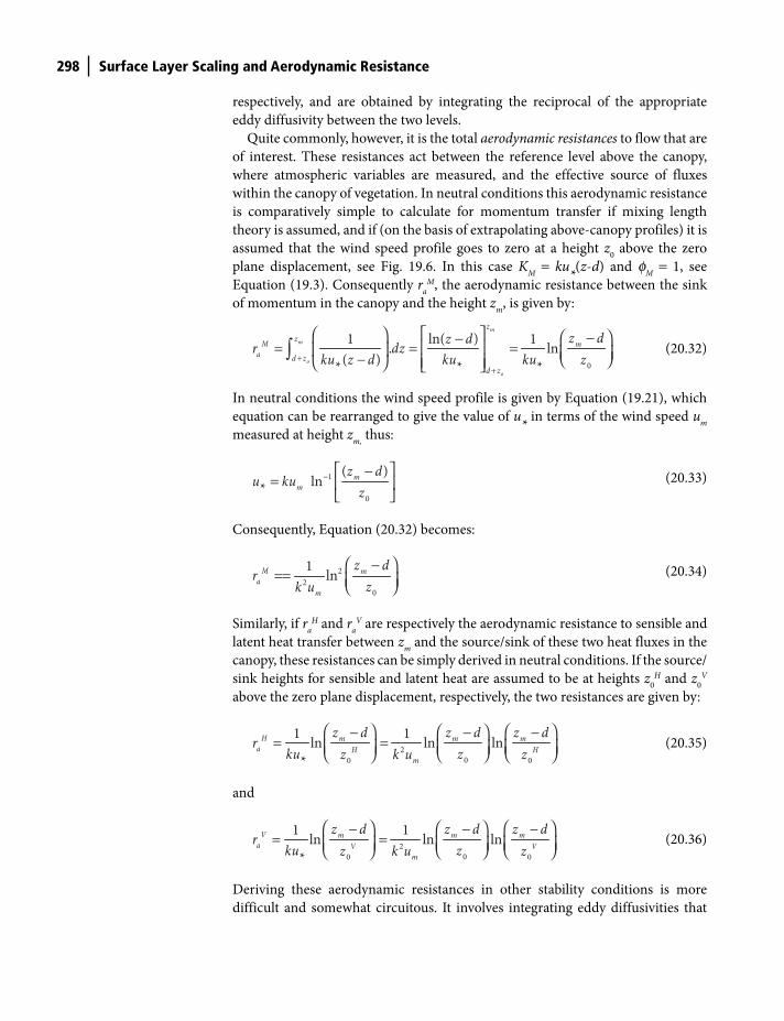
298 Surface Layer Scaling and Aerodynamic Resistance
respectively, and are obtained by integrating the reciprocal of the appropriate
eddy diffusivity between the two levels.
Quite commonly, however, it is the total aerodynamic resistances to flow that are
of interest. These resistances act between the reference level above the canopy,
where atmospheric variables are measured, and the effective source of fluxes
within the canopy of vegetation. In neutral conditions this aerodynamic resistance
is comparatively simple to calculate for momentum transfer if mixing length
theory is assumed, and if (on the basis of extrapolating above-canopy profiles) it is
assumed that the wind speed profile goes to zero at a height z0 above the zero
plane displacement, see Fig. 19.6. In this case KM
= ku*(z-d) and f
M = 1, see
Equation (19.3). Consequently ra
M, the aerodynamic resistance between the sink
of momentum in the canopy and the height zm
, is given by:
++
⎛ ⎞ ⎡ ⎤ ⎛ ⎞−−= = =⎢ ⎥⎜ ⎟ ⎜ ⎟− ⎝ ⎠⎢ ⎥⎝ ⎠ ⎣ ⎦
∫0
1 ln( ) 1. ln
( )* * *
m
m
o
o
zzM m
a d zd z
z dz dr dzku z d ku ku z
(20.32)
In neutral conditions the wind speed profile is given by Equation (19.21), which
equation can be rearranged to give the value of u* in terms of the wind speed u
m
measured at height zm,
thus:
− ⎡ ⎤−= ⎢ ⎥
⎣ ⎦1
0
( ) ln
*m
m
z du ku
z
(20.33)
Consequently, Equation (20.32) becomes:
⎛ ⎞−== ⎜ ⎟⎝ ⎠
2
2
0
1lnM m
am
z dr
zk u
(20.34)
Similarly, if ra
H and ra
V are respectively the aerodynamic resistance to sensible and
latent heat transfer between zm
and the source/sink of these two heat fluxes in the
canopy, these resistances can be simply derived in neutral conditions. If the source/
sink heights for sensible and latent heat are assumed to be at heights z0
H and z0
V
above the zero plane displacement, respectively, the two resistances are given by:
⎛ ⎞ ⎛ ⎞⎛ ⎞− − −= =⎜ ⎟ ⎜ ⎟⎜ ⎟⎝ ⎠⎝ ⎠ ⎝ ⎠2
00 0
1 1ln ln ln
*
H m m ma H H
m
z d z d z dr
ku zz k u z
(20.35)
and
⎛ ⎞ ⎛ ⎞⎛ ⎞− − −= =⎜ ⎟ ⎜ ⎟⎜ ⎟⎝ ⎠⎝ ⎠ ⎝ ⎠2
00 0
1 1ln ln ln
*
V m m ma V V
m
z d z d z dr
ku zz k u z
(20.36)
Deriving these aerodynamic resistances in other stability conditions is more
difficult and somewhat circuitous. It involves integrating eddy diffusivities that
Shuttleworth_c20.indd 298Shuttleworth_c20.indd 298 11/3/2011 6:49:51 PM11/3/2011 6:49:51 PM
Surface Layer Scaling and Aerodynamic Resistance 299
include the flux gradient relationships (i.e. fM
, fH and f
V) which depend on (z-d)/L,
and which therefore depend on the ambient fluxes of sensible heat flux and
momentum. But these in turn are themselves dependent on the resistances that are
being calculated.
Important points in this chapter
● Dimensionless prognostic equation for TKE: in the constant flux layer above
a uniform horizontal surface the prognostic equation for turbulent kinetic
energy (TKE) in the ABL can be re-written in dimensionless form as Equation
(20.1).
● Dimensionless gradients: in the dimensionless prognostic equation for TKE
the fourth term can be used to define fM
, the dimensionless gradient of
wind speed (wind speed gradient normalized to friction velocity and height
above zero plane displacement): similar dimensionless gradients of virtual
potential temperature, fH, and specific humidity, f
V, can also be defined.
● Application of fM
, fH
and fV: in K Theory the reciprocals of the dimension-
less functions fM
, fH and f
V act as multipliers to modify the mixing length
(and thus the efficiency of turbulent transfer) in the surface layer.
● Dimensionless measure of stability: in the dimensionless prognostic equa-
tion for TKE the second term can be used to define, (z-d)/L, a dimensionless
measure of atmospheric stability, in terms of which the dimensionless
functions fM
, fH and f
V (and thus the efficiency of turbulent transfer) can be
parameterized.
● Specification of fM
, fH
and fV: the functional forms of f
M, f
H and f
V with
respect to (z-d)/L are assumed to be universally applicable and field
experiments were carried out to define them: the expressions in Table 20.1
are adopted in this text.
● From kinematic to natural units: before application equations for the
kinematic fluxes of sensible heat, latent heat and momentum derived from
K-Theory must be returned to natural units to give Equations (20.17),
(20.20), and (20.21).
● Resistances: integrating the relationships between fluxes and gradients of
atmospheric variables gives resistances (by analogy with Ohm’s law) that
relate fluxes to the differences in variables between two heights.
● Aerodynamic resistance: total aerodynamic resistance to the turbulent
transfer between a level in the atmosphere and a ‘source’ level in a canopy
can be derived in terms of wind speed, zero plane displacement, and
aerodynamic roughness, e.g., Equations (20.34), (20.35), and (20.36).
Shuttleworth_c20.indd 299Shuttleworth_c20.indd 299 11/3/2011 6:49:52 PM11/3/2011 6:49:52 PM
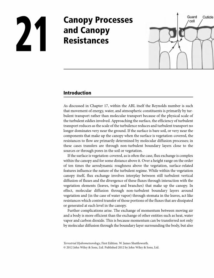
Introduction
As discussed in Chapter 17, within the ABL itself the Reynolds number is such
that movement of energy, water, and atmospheric constituents is primarily by tur-
bulent transport rather than molecular transport because of the physical scale of
the turbulent eddies involved. Approaching the surface, the efficiency of turbulent
transport reduces as the scale of the turbulence reduces and turbulent transport no
longer dominates very near the ground. If the surface is bare soil, or very near the
components that make up the canopy when the surface is vegetation-covered, the
resistances to flow are primarily determined by molecular diffusion processes; in
these cases transfers are through non-turbulent boundary layers close to the
sources or through pores in the soil or vegetation.
If the surface is vegetation-covered, as is often the case, flux exchange is complex
within the canopy and for some distance above it. Over a height range on the order
of ten times the aerodynamic roughness above the vegetation, surface-related
features influence the nature of the turbulent regime. While within the vegetation
canopy itself, flux exchange involves interplay between still turbulent vertical
diffusion of fluxes and the divergence of these fluxes through interaction with the
vegetation elements (leaves, twigs and branches) that make up the canopy. In
effect, molecular diffusion through non-turbulent boundary layers around
vegetation and (in the case of water vapor) through stomata in the leaves, act like
resistances which control transfer of those portions of the fluxes that are dissipated
or generated at each level in the canopy.
Further complications arise. The exchange of momentum between moving air
and a body is more efficient than the exchange of other entities such as heat, water
vapor and carbon dioxide. This is because momentum can be transferred not only
by molecular diffusion through the boundary layer surrounding the body, but also
21 Canopy Processes and Canopy Resistances
Terrestrial Hydrometeorology, First Edition. W. James Shuttleworth.
© 2012 John Wiley & Sons, Ltd. Published 2012 by John Wiley & Sons, Ltd.
Shuttleworth_c21.indd 300Shuttleworth_c21.indd 300 11/3/2011 6:43:06 PM11/3/2011 6:43:06 PM
Canopy Processes and Canopy Resistances 301
by pressure forces. Transfer for other entities is only by molecular diffusion. The
second complication (mentioned in Chapter 19, see Fig. 19.3) is that K Theory is
a poor representation of vertical diffusion inside vegetation canopies. But it is
often still used despite this. Fortunately the negative consequences of this do not
seem to be too severe.
Boundary layer exchange processes
During the 1960s and 1970s there was considerable interest in better quantifying
the aerodynamic behavior of components of natural vegetation inside canopies,
especially leaves. These studies focused on understanding differences in the
effectiveness with which different transferred entities (e.g., momentum, heat,
water vapor and carbon dioxide) are exchanged. Many studies were made inside
wind tunnels, often using artificial replicas of leaves and twigs. There is some
question as to how directly the results obtained in wind tunnels translate into
the real-world environment. Nonetheless, such studies contributed important
background understanding – helpful when considering the whole-canopy behavior
of vegetation stands. This section describes some of the more important results
obtained.
Boundary layers develop over smooth flat surfaces immersed in a moving fluid
such as air. Figure 21.1 illustrates a simple case in which air moving horizontally at
a fixed speed encounters a thin plate (equivalent to a flat leaf, perhaps). A layer of
air, the boundary layer, develops above the plate, which becomes deeper with dis-
tance from the leading edge. There is laminar (as opposed to turbulent) wind flow
inside this boundary layer, the wind speed varying from zero at the surface of the
plate to the speed of the incoming air flow at the edge of the boundary layer.
Momentum is transferred from the moving air through the boundary layer by
molecular diffusion, and the plate experiences a ‘drag’ force as a result.
The interaction between a moving fluid and obstructions in the fluid are
parameterized in terms of the Reynolds number defined in Chapter 17
(Equation 17.28). The velocity of air in a vegetation canopy is typically ∼1.0 m s–1
and a typical dimension of a leaf is ∼0.05 m, giving a Reynolds Number of
order 104.
When the primary exchange between the air flow and the flat plate is by molec-
ular diffusion through a boundary layer, the resulting sheer stress on the plate is
called ‘skin friction’. Experimentally calibrated aerodynamic theory indicates that
the total transfer of momentum per unit area can be estimated from:
ν⎛ ⎞= ρ ⎜ ⎟⎝ ⎠
0.5
0.66 aUUl
t
(21.1)
where U is the speed of the air flow and l is the distance from the edge. If the net
exchange of momentum is expressed in terms of RM
sf, the equivalent
Shuttleworth_c21.indd 301Shuttleworth_c21.indd 301 11/3/2011 6:43:07 PM11/3/2011 6:43:07 PM
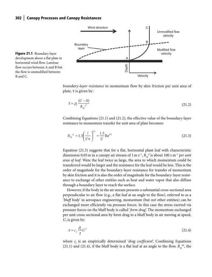
302 Canopy Processes and Canopy Resistances
Wind direction
Boundarylayer
Unmodified flowvelocity
Modified flowvelocity
C
B
A
Dep
th
Velocity
Figure 21.1 Boundary layer
development above a flat plate in
horizontal wind flow. Laminar
flow occurs between A and B but
the flow is unmodified between
B and C.
boundary-layer resistance to momentum flow by skin friction per unit area of
plate, τ is given by:
−=
( 0)a sf
M
UR
t r
(21.2)
Combining Equations (21.1) and (21.2), the effective value of the boundary-layer
resistance to momentum transfer for unit area of plate becomes:
0.5
0.51.51.5 Resf
MlR
U U⎛ ⎞≈ ≈⎜ ⎟ν⎝ ⎠
(21.3)
Equation (21.3) suggests that for a flat, horizontal plant leaf with characteristic
dimension 0.05 m in a canopy air stream of 1 m s–1, RM
sf is about 100 s m–1 per unit
area of leaf. Were the leaf twice as large, the area to which momentum could be
transferred would be larger and the resistance for the leaf would be less. This is the
order of magnitude for the boundary-layer resistance for transfer of momentum
by skin friction and it is also the order of magnitude for the boundary-layer resist-
ance to exchange of other entities such as heat and water vapor that also diffuse
through a boundary layer to reach the surface.
However, if the body in the air stream presents a substantial cross-sectional area
perpendicular to air flow (e.g., a flat leaf at an angle to the flow), referred to as a
‘bluff body’ in aerospace engineering, momentum (but not other entities) can be
exchanged more efficiently via pressure forces. In this case the stress exerted via
pressure forces on the bluff body is called ‘form drag’. The momentum exchanged
per unit cross-sectional area by form drag to a bluff body in air moving at speed,
U, is given by:
= 2
2a
fc Ur
t
(21.4)
where cf is an empirically determined ‘drag coefficient’. Combining Equations
(21.1) and (21.4), if the bluff body is a flat leaf at an angle to the flow, RM
bb, the
Shuttleworth_c21.indd 302Shuttleworth_c21.indd 302 11/3/2011 6:43:08 PM11/3/2011 6:43:08 PM
Canopy Processes and Canopy Resistances 303
boundary-layer resistance to momentum exchange by the form drag exchange
mechanism per unit area of leaf, is given by:
1bbM
f
Rc U
⎛ ⎞≈ ⎜ ⎟⎜ ⎟⎝ ⎠
(21.5)
Note that Equation (21.5) has been written to give the resistance per unit area of
leaf assuming the leaf has two sides. If the canopy air stream velocity is 1 m s–1
and cf = 0.2, R
Mbb is 5 s m–1, which is about an order of magnitude less than the
boundary-layer resistance would be if momentum were transferred solely by
skin friction.
In the case of momentum transfer, it is convenient to combine the effect of skin
friction and bluff body transfer processes in a single drag coefficient, cd, which,
given the form of Equations (21.3) and (21.5), should have the approximate form:
0.5
d fc c nU −≈ + (21.6)
where n is a constant. RM
, the corresponding boundary-layer resistance per unit
area of leaf for momentum transfer by both skin friction and bluff body transfer, is
then given by:
1M
d
Rc U
⎛ ⎞≈ ⎜ ⎟
⎝ ⎠
(21.7)
On the basis of the above discussion, it is clear that the drag coefficient, cd, will
be a strong function of the orientation of the leaf with respect to the wind, a
result that has been demonstrated for model leaves in wind tunnels, see Fig. 21.2,
for example.
The boundary-layer resistance for exchanges other than momentum is deter-
mined by molecular diffusion through a boundary layer. Taking sensible heat, for
example, if the ‘effective’ boundary-layer thickness through which heat has to diffuse
from a leaf to the canopy air stream is d, the boundary-layer resistance per unit area
of leaf for sensible heat, RH, is given by:
=HH
RDd
(21.8)
where DH is the molecular diffusivity for heat. However, because d is not a
measureable quantity, it is preferable to estimate boundary-layer resistance based
on a measureable characteristic dimension, d, of the vegetation instead. For this
reason, the boundary-layer resistance for sensible heat is more conveniently
parameterized in terms of the ‘Nusselt number’ (Nu), defined to be the ratio of a
characteristic dimension of vegetative element, d, to the effective boundary-layer
thickness, d, see Fig. 21.3. In terms of the Nusselt number, the boundary-layer
Shuttleworth_c21.indd 303Shuttleworth_c21.indd 303 11/3/2011 6:43:11 PM11/3/2011 6:43:11 PM
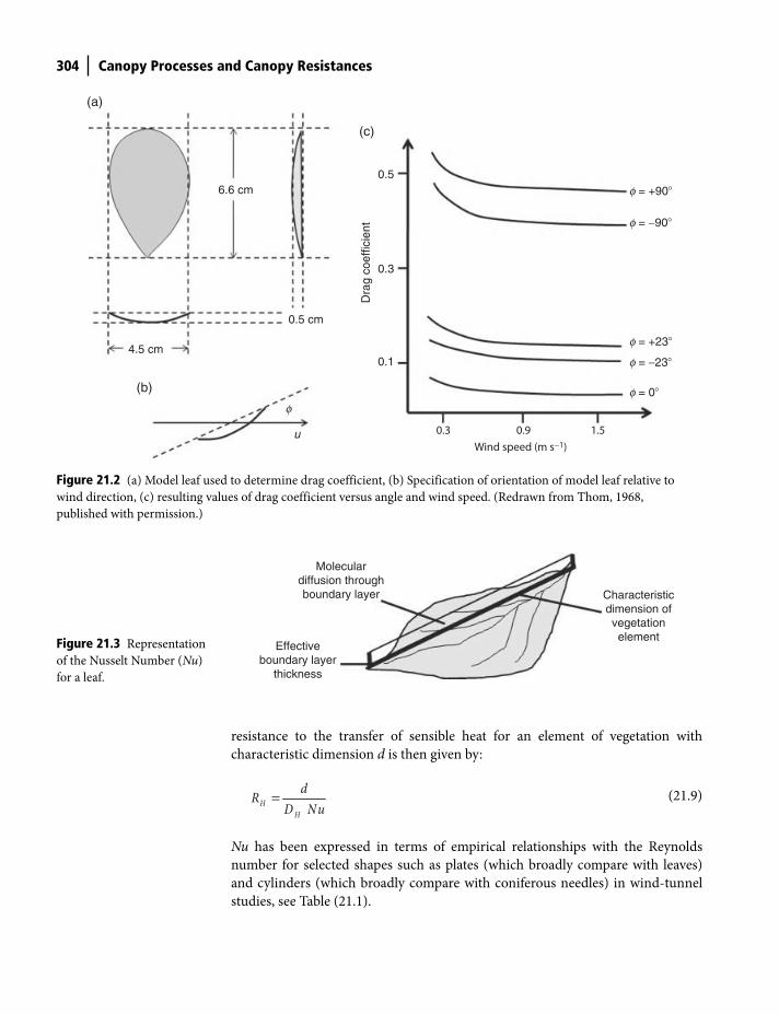
304 Canopy Processes and Canopy Resistances
resistance to the transfer of sensible heat for an element of vegetation with
characteristic dimension d is then given by:
H
H
dRD Nu
=
(21.9)
Nu has been expressed in terms of empirical relationships with the Reynolds
number for selected shapes such as plates (which broadly compare with leaves)
and cylinders (which broadly compare with coniferous needles) in wind-tunnel
studies, see Table (21.1).
0.3 0.9Wind speed (m s−1)
1.5
6.6 cm
0.5 cm
4.5 cm
u
0.5
0.3
0.1D
rag
coef
ficie
nt
f
f = +90�
f = −90�
f = +23�
f = −23�
f = 0�
(c)
(a)
(b)
Figure 21.2 (a) Model leaf used to determine drag coefficient, (b) Specification of orientation of model leaf relative to
wind direction, (c) resulting values of drag coefficient versus angle and wind speed. (Redrawn from Thom, 1968,
published with permission.)
Moleculardiffusion throughboundary layer
Effectiveboundary layer
thickness
Characteristicdimension ofvegetationelementFigure 21.3 Representation
of the Nusselt Number (Nu)
for a leaf.
Shuttleworth_c21.indd 304Shuttleworth_c21.indd 304 11/3/2011 6:43:15 PM11/3/2011 6:43:15 PM
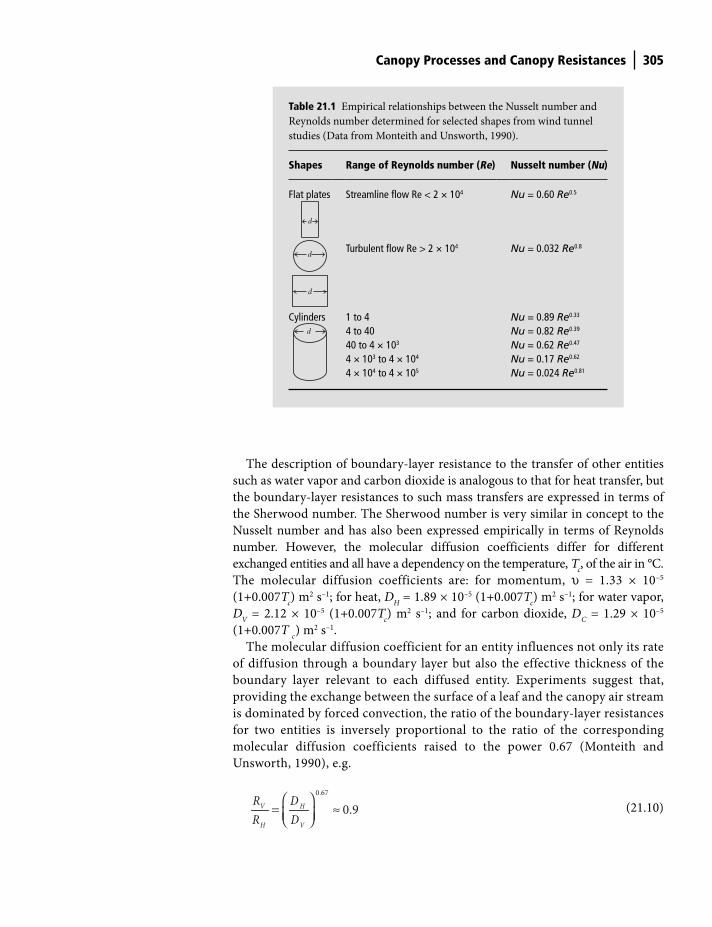
Canopy Processes and Canopy Resistances 305
The description of boundary-layer resistance to the transfer of other entities
such as water vapor and carbon dioxide is analogous to that for heat transfer, but
the boundary-layer resistances to such mass transfers are expressed in terms of
the Sherwood number. The Sherwood number is very similar in concept to the
Nusselt number and has also been expressed empirically in terms of Reynolds
number. However, the molecular diffusion coefficients differ for different
exchanged entities and all have a dependency on the temperature, Tc, of the air in °C.
The molecular diffusion coefficients are: for momentum, υ = 1.33 × 10⁻⁵
(1+0.007Tc) m2 s–1; for heat, D
H = 1.89 × 10⁻⁵ (1+0.007T
c) m2 s–1; for water vapor,
DV = 2.12 × 10⁻⁵ (1+0.007T
c) m2 s–1; and for carbon dioxide, D
C = 1.29 × 10⁻⁵
(1+0.007T c) m2 s–1.
The molecular diffusion coefficient for an entity influences not only its rate
of diffusion through a boundary layer but also the effective thickness of the
boundary layer relevant to each diffused entity. Experiments suggest that,
providing the exchange between the surface of a leaf and the canopy air stream
is dominated by forced convection, the ratio of the boundary-layer resistances
for two entities is inversely proportional to the ratio of the corresponding
molecular diffusion coefficients raised to the power 0.67 (Monteith and
Unsworth, 1990), e.g.
0.67
0.9V H
H V
R DR D
⎛ ⎞= ≈⎜ ⎟⎝ ⎠
(21.10)
Table 21.1 Empirical relationships between the Nusselt number and
Reynolds number determined for selected shapes from wind tunnel
studies (Data from Monteith and Unsworth, 1990).
Shapes Range of Reynolds number (Re) Nusselt number (Nu)
Flat plates
d
Streamline flow Re < 2 × 10⁴ Nu = 0.60 Re0.5
d
d
Turbulent flow Re > 2 × 10⁴ Nu = 0.032 Re0.8
Cylinders 1 to 4 Nu = 0.89 Re0.33
d
4 to 4040 to 4 × 10³
4 × 10³ to 4 × 10⁴
4 × 10⁴ to 4 × 10⁵
Nu = 0.82 Re0.39
Nu = 0.62 Re0.47
Nu = 0.17 Re0.62
Nu = 0.024 Re0.81
Shuttleworth_c21.indd 305Shuttleworth_c21.indd 305 11/3/2011 6:43:16 PM11/3/2011 6:43:16 PM
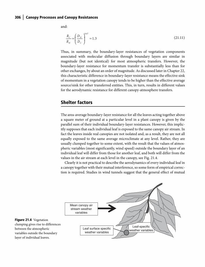
306 Canopy Processes and Canopy Resistances
and:
0.67
1.3C H
H C
R DR D
⎛ ⎞= ≈⎜ ⎟
⎝ ⎠
(21.11)
Thus, in summary, the boundary-layer resistances of vegetation components
associated with molecular diffusion through boundary layers are similar in
magnitude (but not identical) for most atmospheric transfers. However, the
boundary-layer resistance for momentum transfer is substantially less than for
other exchanges, by about an order of magnitude. As discussed later in Chapter 22,
this characteristic difference in boundary-layer resistance means the effective sink
of momentum in a vegetation canopy tends to be higher than the effective average
source/sink for other transferred entities. This, in turn, results in different values
for the aerodynamic resistance for different canopy-atmosphere transfers.
Shelter factors
The area-average boundary-layer resistance for all the leaves acting together above
a square meter of ground at a particular level in a plant canopy is given by the
parallel sum of their individual boundary-layer resistances. However, this implic-
itly supposes that each individual leaf is exposed to the same canopy air stream. In
fact the leaves inside real canopies are not isolated and, as a result, they are not all
equally exposed to the same average microclimate at any level. Rather, they are
usually clumped together to some extent, with the result that the values of atmos-
pheric variables (most significantly, wind speed) outside the boundary layer of an
individual leaf will differ from those for another leaf, and both will differ from the
values in the air stream at each level in the canopy, see Fig. 21.4.
Clearly it is not practical to describe the aerodynamics of every individual leaf in
a canopy together with their mutual interference, so some form of empirical correc-
tion is required. Studies in wind tunnels suggest that the general effect of mutual
Leaf-specificweather variables
Mean canopy airstream weather
variables
Leaf surface specificweather variables
Figure 21.4 Vegetation
clumping gives rise to differences
between the atmospheric
variables outside the boundary
layer of individual leaves.
Shuttleworth_c21.indd 306Shuttleworth_c21.indd 306 11/3/2011 6:43:18 PM11/3/2011 6:43:18 PM
Canopy Processes and Canopy Resistances 307
interference is that the effective value of the area-average boundary-layer resistance
is higher than would be calculated by a parallel summation of the values for indi-
vidual leaves. One way to approximately describe the effect of mutual interference
is to assume the increase in the effective area-average boundary-layer resistance can
be allowed for by including a simple multiplicative factor called a shelter factor.
The contribution to a canopy flux at a particular level in a canopy might be
assumed proportional to the difference between the mean value of an atmospheric
variable in the canopy air stream and the mean value of that same variable at the
surface of the vegetation elements (leaves) at that level. The equations describing
the contributions to the sensible heat flux, latent heat flux, and momentum flux
generated or lost at level z are then respectively given by:
( )( )
( )
s zH z a p
H z
T Tc
R−
=d r
(21.12)
λ
−=
( )( )
( )
a p s zE z
V z
c e eR
rd
g
(21.13)
−=
(0 )( )
( )
zz a
M z
uRtd r
(21.14)
where Tz, e
z, and u
z are the temperature, vapor pressure, and wind speed of the
mean canopy air stream at level z, respectively, and Ts and e
s are the mean values of
the temperature and vapor pressure at the surface of the leaves at level z,. In
Equations (21.12) to (21.14), the mean boundary-layer resistances for heat, water
vapor, and momentum for the N leaves in a small height range dz around the level
z are respectively defined by:
−
=
⎡ ⎤= ⎢ ⎥
⎢ ⎥⎣ ⎦∑
1
1
( )
H
Ni
H z H ii
AR P
R
(21.15)
−
=
⎡ ⎤= ⎢ ⎥
⎣ ⎦∑
1
1
( )N
iV z V i
i V
AR P
R
(21.16)
−
=
⎡ ⎤= ⎢ ⎥
⎢ ⎥⎣ ⎦∑
1
1
( )
M
Ni
M z M ii
AR P
R
(21.17)
where Ai is the area and R
Hi, R
Vi, and R
Mi are the boundary-layer resistances per
unit area of the i th leaf, and PH, P
V, and P
M are shelter factors for heat, water vapor
and momentum, respectively. Because it is the reciprocal of the boundary-layer
Shuttleworth_c21.indd 307Shuttleworth_c21.indd 307 11/3/2011 6:43:19 PM11/3/2011 6:43:19 PM
308 Canopy Processes and Canopy Resistances
resistance, the boundary-layer conductance, that scales linearly with the area of
leaf, when calculating the mean boundary-layer resistance it is necessary to first
calculate the area-weighted average of the reciprocal of the boundary resistance
for each leaf, and then to take the reciprocal of that mean.
The numerical values of shelter factors are poorly defined and are likely to vary
greatly with canopy structure but they are believed to be of the order 2 to 3. The
fact that shelter factors are so large and so poorly defined compromises the value
of early wind tunnel research into the boundary-layer resistance for individual
leaves to some extent. However, basic knowledge of the order of magnitude of
boundary-layer resistances found in those studies, and the understanding they
gave of the difference between boundary-layer resistance for momentum transfer
and for other transfers, is important when writing equations describing the whole-
canopy aerodynamic resistance, as discussed in the next chapter.
Stomatal resistance
At each level in the canopy, contributions to the overall canopy exchange of sensible
heat flux originate from the exposed surface of the vegetation elements present at
that level, and arise because of the difference between the surface temperature of
the vegetation and the temperature of the canopy air stream. As just discussed, the
magnitude of the contributions is controlled by the mean boundary-layer resistance
of the vegetation elements at each level.
Plant cells are about 90% water and would quickly desiccate and die if exposed
to an unsaturated atmosphere. For this reason, plants seek to retain water content
using surface layers that are resistant to water loss. Most leaves, for example, have
a waxy cuticle that inhibits the loss of gases such as water vapor and carbon
dioxide from their surface. But, if plants are to grow, they need to allow the cells
within leaves not only to absorb photosynthetically active radiation but also to
have access to the CO2 present in the atmosphere. They do this by gas exchange,
with internal cells gaining access to CO2 through small pores in the leaf surfaces
called ‘stomata’ which can be opened in environmental conditions favorable for
photosynthesis.
The same stomata that allow carbon dioxide to enter leaves also allow water
vapor evaporated from the moist cell walls inside the leaf to escape to the
atmosphere. Consequently, if the outside surface of vegetation canopy is dry (not
wet as after rainfall), the primary source of water leaving plants is from cells inside
leaves. This water vapor diffusing by molecular diffusion from sub-stomatal
cavities through stomata to the leaf surface and the need to diffuse through narrow
stomata inhibits the rate of water vapor flow, depending on the extent to which the
plant stomata are open. This inhibition on flow is represented in equations and
models by a resistance, the stomatal resistance, rST
, to vapor flow from inside to
just outside the leaf, see Fig. 21.5. Thus, the stomatal resistance per unit area of leaf
is used in much the same way that boundary-layer resistance is used to represent
Shuttleworth_c21.indd 308Shuttleworth_c21.indd 308 11/3/2011 6:43:25 PM11/3/2011 6:43:25 PM
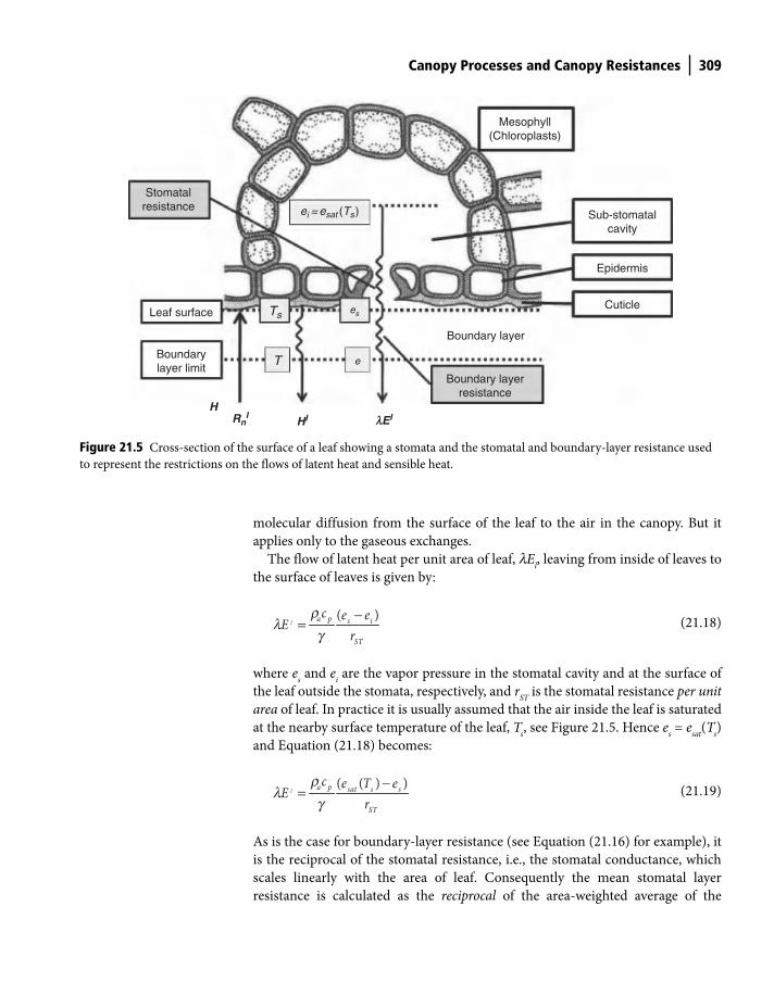
Canopy Processes and Canopy Resistances 309
molecular diffusion from the surface of the leaf to the air in the canopy. But it
applies only to the gaseous exchanges.
The flow of latent heat per unit area of leaf, lEl, leaving from inside of leaves to
the surface of leaves is given by:
( )l a p s i
ST
c e eEr−
=r
lg
(21.18)
where es and e
i are the vapor pressure in the stomatal cavity and at the surface of
the leaf outside the stomata, respectively, and rST
is the stomatal resistance per unit
area of leaf. In practice it is usually assumed that the air inside the leaf is saturated
at the nearby surface temperature of the leaf, Ts, see Figure 21.5. Hence e
s = e
sat(T
s)
and Equation (21.18) becomes:
( ( ) )l a p sat s s
ST
c e T eEr
−=
rl
g
(21.19)
As is the case for boundary-layer resistance (see Equation (21.16) for example), it
is the reciprocal of the stomatal resistance, i.e., the stomatal conductance, which
scales linearly with the area of leaf. Consequently the mean stomatal layer
resistance is calculated as the reciprocal of the area-weighted average of the
Boundary layer
Boundary layerresistance
Stomatalresistance
Leaf surface
Boundarylayer limit
T
Ts
RnI
HI lEI
es
e
ei =esat (Ts)
Cuticle
Epidermis
Sub-stomatalcavity
Mesophyll(Chloroplasts)
H
Figure 21.5 Cross-section of the surface of a leaf showing a stomata and the stomatal and boundary-layer resistance used
to represent the restrictions on the flows of latent heat and sensible heat.
Shuttleworth_c21.indd 309Shuttleworth_c21.indd 309 11/3/2011 6:43:25 PM11/3/2011 6:43:25 PM

310 Canopy Processes and Canopy Resistances
reciprocal of stomatal resistance for each leaf. For example, ( )st zr , the mean stomatal
resistance per unit leaf area of the N leaves in a (small) height range δz around the
level z is given by:
1
1
( )N
ist z i
i ST
Arr
−
=
⎡ ⎤= ⎢ ⎥
⎣ ⎦∑
(21.20)
Energy budget of a dry leaf
On a per leaf area basis, the sensible heat and latent heat flux exchanges with the
surface of a leaf shown in Figure 21.5 are given by:
( )l s za p
H
T TH cR−
= r
(21.21)
and:
( ( ) )a pl sat s
V ST
c e T eER r
−=
+r
lg
(21.22)
Assuming the energy stored in the leaf is negligible, the surface energy budget is
given by:
l l lnE H R+ =l
(21.23)
where Rn
l is the energy falling as net radiation per unit area of leaf.
If the equivalent linear rate of change in saturated vapor pressure between Ts
and T, Δ, is defined by:
( ) ( )sat s sat
s
e T e TT T
−Δ =
−
(21.24)
then rearranging Equation (21.23), and substituting first Equations (21.21) and
then Equation (21.24) gives:
( ( ) ( ))l l sat s satn a p
H
e T e TE R cR−
= −Δ
l r
(21.25)
which equation can be written as:
Shuttleworth_c21.indd 310Shuttleworth_c21.indd 310 11/3/2011 6:43:27 PM11/3/2011 6:43:27 PM
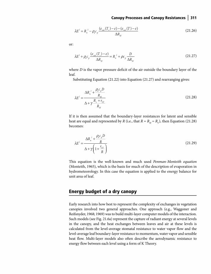
Canopy Processes and Canopy Resistances 311
( ( ) ) ( ( ) )l l sat s satn a p
H
e T e e T eE R cR
− − −= −
Δl r
(21.26)
or:
( ( ) )l lsat sa p n p
H H
e T e DE c R cR R
−+ = +
Δ Δl r r
(21.27)
where D is the vapor pressure deficit of the air outside the boundary layer of the
leaf.
Substituting Equation (21.22) into Equation (21.27) and rearranging gives:
a pln
l H
v ST
H
c DR
RE R rR
Δ +=
+Δ +
r
lg
(21.28)
If it is then assumed that the boundary-layer resistances for latent and sensible
heat are equal and represented by R (i.e., that R = RH = R
V), then Equation (21.28)
becomes:
1
a pln
l
ST
c DR
RErR
Δ +=
⎛ ⎞Δ + +⎜ ⎟⎝ ⎠
r
lg
(21.29)
This equation is the well-known and much used Penman-Monteith equation
(Monteith, 1965), which is the basis for much of the description of evaporation in
hydrometeorology. In this case the equation is applied to the energy balance for
unit area of leaf.
Energy budget of a dry canopy
Early research into how best to represent the complexity of exchanges in vegetation
canopies involved two general approaches. One approach (e.g., Waggoner and
Reifsnyder, 1968; 1969) was to build multi-layer computer models of the interaction.
Such models (see Fig. 21.6a) represent the capture of radiant energy at several levels
in the canopy, and the heat exchanges between leaves and air at these levels is
calculated from the level-average stomatal resistance to water vapor flow and the
level-average leaf boundary-layer resistance to momentum, water vapor and sensible
heat flow. Multi-layer models also often describe the aerodynamic resistance to
energy flow between each level using a form of K Theory.
Shuttleworth_c21.indd 311Shuttleworth_c21.indd 311 11/3/2011 6:43:34 PM11/3/2011 6:43:34 PM
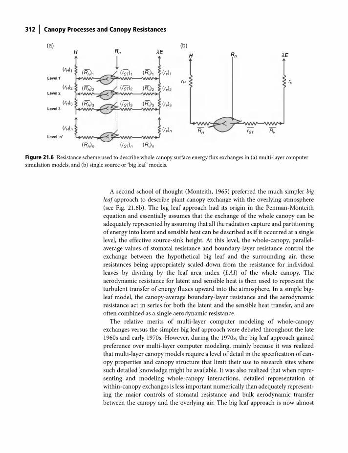
312 Canopy Processes and Canopy Resistances
A second school of thought (Monteith, 1965) preferred the much simpler big
leaf approach to describe plant canopy exchange with the overlying atmosphere
(see Fig. 21.6b). The big leaf approach had its origin in the Penman-Monteith
equation and essentially assumes that the exchange of the whole canopy can be
adequately represented by assuming that all the radiation capture and partitioning
of energy into latent and sensible heat can be described as if it occurred at a single
level, the effective source-sink height. At this level, the whole-canopy, parallel-
average values of stomatal resistance and boundary-layer resistance control the
exchange between the hypothetical big leaf and the surrounding air, these
resistances being appropriately scaled-down from the resistance for individual
leaves by dividing by the leaf area index (LAI) of the whole canopy. The
aerodynamic resistance for latent and sensible heat is then used to represent the
turbulent transfer of energy fluxes upward into the atmosphere. In a simple big-
leaf model, the canopy-average boundary-layer resistance and the aerodynamic
resistance act in series for both the latent and the sensible heat transfer, and are
often combined as a single aerodynamic resistance.
The relative merits of multi-layer computer modeling of whole-canopy
exchanges versus the simpler big leaf approach were debated throughout the late
1960s and early 1970s. However, during the 1970s, the big leaf approach gained
preference over multi-layer computer modeling, mainly because it was realized
that multi-layer canopy models require a level of detail in the specification of can-
opy properties and canopy structure that limit their use to research sites where
such detailed knowledge might be available. It was also realized that when repre-
senting and modeling whole-canopy interactions, detailed representation of
within-canopy exchanges is less important numerically than adequately represent-
ing the major controls of stomatal resistance and bulk aerodynamic transfer
between the canopy and the overlying air. The big leaf approach is now almost
H Rn lEH Rn lE
Level 1
Level 2
Level 3
Level ‘n’
(rH)1
(rH)2
(rH)3
(rH)n
(RH)n
(RH)3
(RH)2
(RH)1
(rST)n
(rST)3
(Rv)n
(rST)2
(rST)1
(Rv)3
(Rv)2
(Rv)1
(rv)3
(rv)n
(rv)2
rH rv
RH rST Rv
(rv)1
(a) (b)
Figure 21.6 Resistance scheme used to describe whole canopy surface energy flux exchanges in (a) multi-layer computer
simulation models, and (b) single source or ‘big leaf ’ models.
Shuttleworth_c21.indd 312Shuttleworth_c21.indd 312 11/3/2011 6:43:37 PM11/3/2011 6:43:37 PM
Canopy Processes and Canopy Resistances 313
universally used in hydrological and meteorological modeling, sometimes, but not
always, with the inclusion of below canopy fluxes from the soil, which may also be
calculated using the Penman-Monteith Equation applied at the soil surface.
If below canopy fluxes are neglected (they can be small below a fully developed
vegetation canopy), the representation of whole-canopy surface energy balance in
the big leaf representation can be calculated by a whole-canopy version of the
Penman-Monteith Equation. In this case (see Fig. 21.7) the equations representing
the whole-canopy exchanges of sensible heat, H, and latent heat flux, λE, are
respectively:
( )s refa p H
a
T TH c
r−
= r
(21.30)
and:
( ( ) )a p sat s refH
a s
c e T eE
r r−
=+
rl
g
(21.31)
where Tref
and eref
are the temperature and vapor pressure at a reference level above
the canopy, Ts is the canopy-average leaf surface temperature, r
s is the canopy-
average leaf stomatal resistance (often called the ‘surface resistance’), and ra
H and
ra
V are the aerodynamic resistances for the transfer of water vapor and sensible
heat (which include both the canopy-average leaf boundary-layer resistances and
the aerodynamic transfer resistance for turbulent transport between the effective
Figure 21.7 The whole canopy
single source model used to
derive the whole canopy version
of the Penman-Monteith
equation.
Shuttleworth_c21.indd 313Shuttleworth_c21.indd 313 11/3/2011 6:43:38 PM11/3/2011 6:43:38 PM
314 Canopy Processes and Canopy Resistances
source in the canopy and the reference level.) In a whole-canopy representation,
the total energy available to support sensible and latent heat transfer is given by:
+ =E H Al (21.32)
where A, the available energy, in addition to net radiation, includes allowance for
soil heat flux, G, and the physical and biochemical storage in the canopy, S and P,
respectively (see Chapter 4).
Equations (21.30), (21.31), and (21.32) are analogous to Equations (21.21),
(21.22), and (21.23), respectively, and the derivation of the whole-canopy Penman-
Monteith Equation therefore follows by direct analogy with that for unit area of
leaf given above. Assuming ra = r
aH = r
aV, the resulting equation takes the form:
1
a p ref
a
s
a
c DA
rErr
Δ +=
⎛ ⎞Δ + +⎜ ⎟⎝ ⎠
r
lg
(21.33)
where Dref
is the observed VPD at the reference level above the canopy.
Important points in this chapter
● Turbulent and non-turbulent controls: within a vegetation canopy flux
exchange involves interplay between turbulent vertical diffusion of fluxes
and the divergence of these fluxes through non-turbulent interaction with
the vegetation elements that make up the canopy. Resistances associated with
molecular diffusion through boundary layers and stomata control the
dissipation or generation of portions of the fluxes at each level in the canopy.
● Skin friction and bluff body transfer: all fluxes from the canopy air stream to
leaves can occur by skin friction transfer (i.e. by molecular diffusion through
the non-turbulent boundary layers surrounding leaves), but momentum can
also be transferred more efficiently by pressure forces in bluff body transfer,
hence the boundary-layer resistance for momentum is about an order of
magnitude less than for other transfers, depending on the orientation of
the leaf.
● Influence of molecular diffusion coefficient: when boundary-layer resist-
ance is controlled by skin friction transfer the relevant molecular transfer
coefficient controls both rate of diffusion and thickness of the boundary
layer, hence the ratio of the boundary-layer resistances for two transfers is
inversely proportional to the ratio of their molecular diffusion coefficients
raised to the power 0.67.
Shuttleworth_c21.indd 314Shuttleworth_c21.indd 314 11/3/2011 6:43:40 PM11/3/2011 6:43:40 PM
Canopy Processes and Canopy Resistances 315
● Shelter factors: mutual sheltering of leaves in a canopy raises the effective
value of boundary-layer resistances by empirical shelter factors of the order
of 2 to 3.
● Stomatal resistance: in dry canopies water mainly evaporates inside the
leaves so, in addition to boundary-layer resistance, latent heat (and CO2) flux
also has to pass through a stomatal resistance associated molecular diffusion
through the plants’ stomata.
● Single leaf Penman-Monteith equation: simultaneously solving the energy
balance equation for a single leaf and equations that control the rate of diffu-
sion of heat fluxes through boundary-layer resistances and stomatal resistance
gives the Penman-Monteith equation for a single leaf, see Equation (21.29).
● Whole-canopy Penman-Monteith equation: the single source or ‘big leaf ’
representation of energy balance for a canopy (with surface resistance taken
as the canopy average of all stomatal resistances acting in parallel, and
aerodynamic resistance as the sum of turbulent transfer resistance and canopy
average boundary-layer resistance acting in series) gives the whole-canopy
Penman-Monteith Equation using a derivation analogous to that for a single
leaf, see Equation (21.33).
References
Monteith, J.L. (1965) Evaporation and environment. Symposium of the Society for
Experimental Biology 19, 205–234; republished in Gash, J.H.C. and Shuttleworth, W.J.,
(2007) Benchmark Papers in Hydrology: Evaporation. IAHS Press, Wallingford, 521p.
Monteith, J.L. and Unsworth, M.H. (1990) Principles of Environmental Physics. Edward
Arnold, London, p. 291.
Thom, A.S. (1968) The exchange of momentum, mass, and heat between an artificial leaf
and the airflow in a wind-tunnel. Quarterly Journal of the Royal Meteorological Society,
94, 44–55.
Waggoner, P.E. and Reifsnyder, W.E. (1968) Simulation of the temperature, humidity, and
evaporation profiles in a leaf canopy. Journal of Applied Meteorology, 7, 400–409.
Waggoner, P.E. and Reifsnyder, W.E. (1969) Simulation of the microclimate in a forest.
Forest Science, 15, 37–40.
Shuttleworth_c21.indd 315Shuttleworth_c21.indd 315 11/3/2011 6:43:42 PM11/3/2011 6:43:42 PM
Introduction
Real vegetation canopies are extended three-dimensional entities. Even in the
case of agricultural crops in the middle of their growth season (arguably the
most uniform vegetation cover), assuming the whole-canopy interaction can
be adequately represented as if it occurred at a single effective source/sink level as
in the Penman-Monteith equation requires some faith, because observed profiles
of atmospheric variables change substantially with height, see Fig. 22.1.
However, as already discussed in Chapter 21 (see Fig. 21.6 and associated text),
the alternative approach of using numerical models to simulate multi-level
exchanges is impractical, given that such models require detailed site- and time-
specific knowledge of canopy structure that is rarely available. Multi-layer canopy
models also usually make the problematic assumption that K Theory applies
within plant canopies, as discussed in Chapter 19 (see Fig. 19.3). But, given the
necessity to resort to the single source/sink assumption, how can the knowledge
of in-canopy processes discussed in the last chapter be used to best advantage in a
big leaf model? This is one of the topics considered in this chapter.
When the big leaf representation of the plant–atmosphere interactions and
Penman-Monteith equation are adopted, surface exchanges depend on the values
of weather variables at some reference level in the ABL. However, the discussion of
ABL development given in Chapter 18 indicates that atmospheric variables in the
ABL (including those at the reference level) are themselves partly determined by
surface energy inputs. Thus, because the air in the ABL is not totally ‘free’ but rather
often partly ‘contained’ by an inversion layer, feedback processes can come in to
play, with surface exchanges not only determined by, but also in part determining,
the value of near surface weather variables. The effect of ABL feedbacks on area-
average surface exchange is also discussed in this chapter.
22 Whole-Canopy Interactions
Terrestrial Hydrometeorology, First Edition. W. James Shuttleworth.
© 2012 John Wiley & Sons, Ltd. Published 2012 by John Wiley & Sons, Ltd.
Shuttleworth_c22.indd 316Shuttleworth_c22.indd 316 11/3/2011 6:41:51 PM11/3/2011 6:41:51 PM
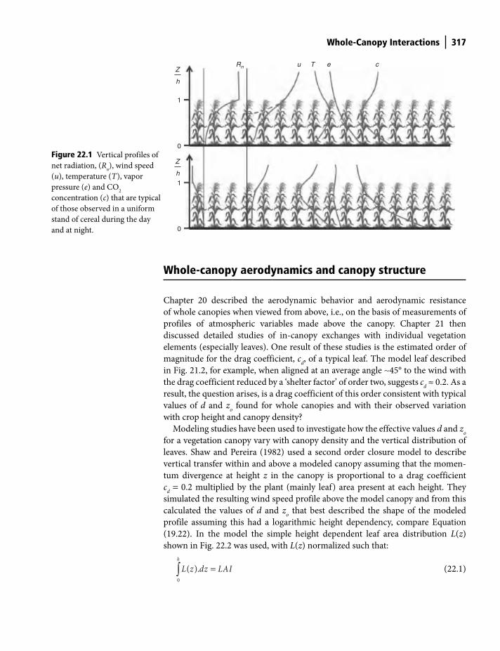
Whole-Canopy Interactions 317
Whole-canopy aerodynamics and canopy structure
Chapter 20 described the aerodynamic behavior and aerodynamic resistance
of whole canopies when viewed from above, i.e., on the basis of measurements of
profiles of atmospheric variables made above the canopy. Chapter 21 then
discussed detailed studies of in-canopy exchanges with individual vegetation
elements (especially leaves). One result of these studies is the estimated order of
magnitude for the drag coefficient, cd, of a typical leaf. The model leaf described
in Fig. 21.2, for example, when aligned at an average angle ∼45° to the wind with
the drag coefficient reduced by a ‘shelter factor’ of order two, suggests cd ≈ 0.2. As a
result, the question arises, is a drag coefficient of this order consistent with typical
values of d and zo found for whole canopies and with their observed variation
with crop height and canopy density?
Modeling studies have been used to investigate how the effective values d and zo
for a vegetation canopy vary with canopy density and the vertical distribution of
leaves. Shaw and Pereira (1982) used a second order closure model to describe
vertical transfer within and above a modeled canopy assuming that the momen-
tum divergence at height z in the canopy is proportional to a drag coefficient
cd = 0.2 multiplied by the plant (mainly leaf) area present at each height. They
simulated the resulting wind speed profile above the model canopy and from this
calculated the values of d and zo that best described the shape of the modeled
profile assuming this had a logarithmic height dependency, compare Equation
(19.22). In the model the simple height dependent leaf area distribution L(z)
shown in Fig. 22.2 was used, with L(z) normalized such that:
0
( ).h
L z dz LAI=∫ (22.1)
Rn
1
0
1
0
u T e cZ
h
Z
h
Figure 22.1 Vertical profiles of
net radiation, (Rn), wind speed
(u), temperature (T), vapor
pressure (e) and CO2
concentration (c) that are typical
of those observed in a uniform
stand of cereal during the day
and at night.
Shuttleworth_c22.indd 317Shuttleworth_c22.indd 317 11/3/2011 6:41:52 PM11/3/2011 6:41:52 PM
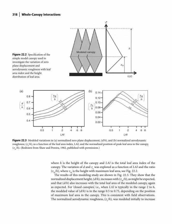
318 Whole-Canopy Interactions
where h is the height of the canopy and LAI is the total leaf area index of the
canopy. The variation of d and zo was explored as a function of LAI and the ratio
(zM
/h), where zM
is the height with maximum leaf area, see Fig. 22.2.
The results of this modeling study are shown in Fig. 22.3. They show that the
normalized displacement height, (d/h), increases with (zM
/h), as might be expected,
and that (d/h) also increases with the total leaf area of the modeled canopy, again
as expected. For ‘closed canopies’, i.e., when LAI is typically in the range 2 to 6,
the modeled value of (d/h) is in the range 0.5 to 0.75, depending on the position
of maximum leaf area in the canopy. This is consistent with field observations.
The normalized aerodynamic roughness, (zo/h), was modeled initially to increase
Modeled canopy
Z
h
zm
L(z)
Figure 22.2 Specification of the
simple model canopy used to
investigate the variation of zero
plane displacement and
aerodynamic roughness with leaf
area index and the height
distribution of leaf area.
0.8
0.7
0.6
0.5
0.4
0.5 1 2
LAI
4 6 8
0.8
0.6
0.4
0.2
(a)zM
h
d
h
0.5 1 2
LAI
4 6 8
0.20.40.6
0.8
(b)zM
h
0.02
0.04
0.06
0.08
0.10
0.12
0.14
z0
h
Figure 22.3 Modeled variations in (a) normalized zero plane displacement, (d/h), and (b) normalized aerodynamic
roughness, (zo/h), as a function of the leaf area index, LAI, and the normalized position of peak leaf area in the canopy,
(zm
/h). (Redrawn from Shaw and Pereira, 1982, published with permission.)
Shuttleworth_c22.indd 318Shuttleworth_c22.indd 318 11/3/2011 6:41:53 PM11/3/2011 6:41:53 PM
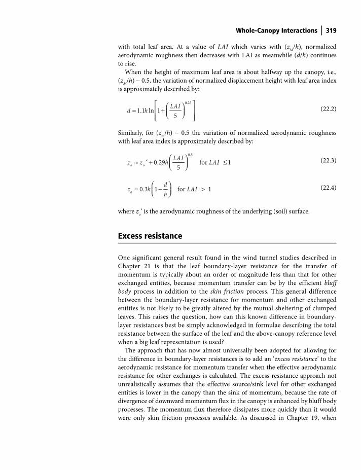
Whole-Canopy Interactions 319
with total leaf area. At a value of LAI which varies with (zM
/h), normalized
aerodynamic roughness then decreases with LAI as meanwhile (d/h) continues
to rise.
When the height of maximum leaf area is about halfway up the canopy, i.e.,
(zM
/h) ∼ 0.5, the variation of normalized displacement height with leaf area index
is approximately described by:
0.25
1.1 ln 15
LAId h⎡ ⎤⎛ ⎞≈ +⎢ ⎥⎜ ⎟⎝ ⎠⎢ ⎥⎣ ⎦
(22.2)
Similarly, for (zm
/h) ∼ 0.5 the variation of normalized aerodynamic roughness
with leaf area index is approximately described by:
0.5
0.29 for 15
o oLAIz z h LAI⎛ ⎞≈ + ≤⎜ ⎟⎝ ⎠
¢ (22.3)
0.3 1 for 1odz h LAIh
⎛ ⎞≈ − >⎜ ⎟⎝ ⎠
(22.4)
where zo’ is the aerodynamic roughness of the underlying (soil) surface.
Excess resistance
One significant general result found in the wind tunnel studies described in
Chapter 21 is that the leaf boundary-layer resistance for the transfer of
momentum is typically about an order of magnitude less than that for other
exchanged entities, because momentum transfer can be by the efficient bluff
body process in addition to the skin friction process. This general difference
between the boundary-layer resistance for momentum and other exchanged
entities is not likely to be greatly altered by the mutual sheltering of clumped
leaves. This raises the question, how can this known difference in boundary-
layer resistances best be simply acknowledged in formulae describing the total
resistance between the surface of the leaf and the above-canopy reference level
when a big leaf representation is used?
The approach that has now almost universally been adopted for allowing for
the difference in boundary-layer resistances is to add an ‘excess resistance’ to the
aerodynamic resistance for momentum transfer when the effective aerodynamic
resistance for other exchanges is calculated. The excess resistance approach not
unrealistically assumes that the effective source/sink level for other exchanged
entities is lower in the canopy than the sink of momentum, because the rate of
divergence of downward momentum flux in the canopy is enhanced by bluff body
processes. The momentum flux therefore dissipates more quickly than it would
were only skin friction processes available. As discussed in Chapter 19, when
Shuttleworth_c22.indd 319Shuttleworth_c22.indd 319 11/3/2011 6:41:54 PM11/3/2011 6:41:54 PM
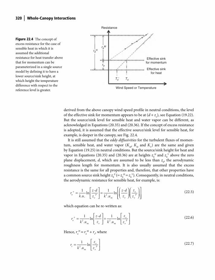
320 Whole-Canopy Interactions
derived from the above canopy wind speed profile in neutral conditions, the level
of the effective sink for momentum appears to be at (d + zo), see Equation (19.22).
But the source/sink level for sensible heat and water vapor can be different, as
acknowledged in Equations (20.35) and (20.36). If the concept of excess resistance
is adopted, it is assumed that the effective source/sink level for sensible heat, for
example, is deeper in the canopy, see Fig. 22.4.
It is still assumed that the eddy diffusivities for the turbulent fluxes of momen-
tum, sensible heat, and water vapor (KM
, KH and K
V) are the same and given
by Equation (19.25) in neutral conditions. But the source/sink height for heat and
vapor in Equations (20.35) and (20.36) are at heights z0
H and z0
V above the zero
plane displacement, d, which are assumed to be less than z0, the aerodynamic
roughness length for momentum. It is also usually assumed that the excess
resistance is the same for all properties and, therefore, that other properties have
a common source sink height z0
P (= z0
H = z0
V). Consequently, in neutral conditions,
the aerodynamic resistance for sensible heat, for example, is:
2
* m
1 - 1 - ln ln
. .
H oa P P
oo o
zz d z drk u zz k u z
⎡ ⎤⎡ ⎤ ⎛ ⎞⎛ ⎞= = ⎢ ⎥⎢ ⎥ ⎜ ⎟⎜ ⎟⎝ ⎠ ⎝ ⎠⎢ ⎥⎣ ⎦ ⎣ ⎦
(22.5)
which equation can be re-written as:
2 2
m m
1 - 1 ln ln
. .
H oa P
o o
zz drzk u k u z
⎡ ⎤⎡ ⎤= + ⎢ ⎥⎢ ⎥
⎣ ⎦ ⎣ ⎦ (22.6)
Hence, ra
H = ra
M + re, where
2
m
1 ln
.
oe P
o
zr
k u z⎡ ⎤
= ⎢ ⎥⎣ ⎦
(22.7)
Resistance
Effective sinkfor momentum
Effective sinkfor heat
Wind Speed or Temperature
To’ To
re
raM
raH
Figure 22.4 The concept of
excess resistance for the case of
sensible heat in which it is
assumed the additional
resistance for heat transfer above
that for momentum can be
parameterized in a single source
model by defining it to have a
lower source/sink height, at
which height the temperature
difference with respect to the
reference level is greater.
Shuttleworth_c22.indd 320Shuttleworth_c22.indd 320 11/3/2011 6:41:57 PM11/3/2011 6:41:57 PM

Whole-Canopy Interactions 321
The value of re has been measured in field studies for a wide range of natural,
permeable, fibrous surfaces. Figure 22.5 shows measured values of ln(z0/z
H) as a
function of the roughness Reynolds number (defined by Re* = (u*
zo)/ν) for a wide
range of surface types. Thus, the observed magnitude of ln(z0/z
H) for the fibrous
vegetation surfaces is of order two which, given the very substantial observational
variability in these measurements, roughly corresponds to z0
P ≈ (z0 / 10).
Substituting z0
P ≈ (z0 / 10) into Equations (20.35) while allowing the possibility
that the measurement height for temperature, zm′, might differ from that for wind
speed, zm
, gives:
⎛ ⎞⎛ ⎞− −= = ⎜ ⎟⎜ ⎟⎝ ⎠ ⎝ ⎠2
0 0
1ln ln
10
H m ma
m
z d z dr
z zk u¢
(22.8)
Commonly the whole canopy aerodynamic resistance, ra, is assumed to be the
same for sensible and latent heat transfer and given by:
2
0 0
1ln ln
10
V H m ma a a
m
z d z dr r r
z zk u⎛ ⎞⎛ ⎞− −
= = = ⎜ ⎟⎜ ⎟⎝ ⎠ ⎝ ⎠¢ (22.9)
Roughness sublayer
The turbulent interaction of the atmosphere can be parameterized in one dimen-
sion through the aerodynamic parameters z0 and d, and similarity theory is
assumed to be independent of the nature of the underlying surface. However, field
observations over tall vegetation suggest that very close to the surface (typically for
heights up to 50 z0) this is not true and that surface-related features (such as the
‘wakes’ generated by individual plants) can alter the local efficiency of turbulent
10010 1000 10000 100000
0
−2
2
4
Re*
(1)
(2)(3)
(4)
(5)
(6)
(7)
InZo
ZoH
Figure 22.5 Observed values of
ln(z0/z
H) as a function of the
roughness Reynolds number
Re* = (u*
zo)/ν for surface types
(1) vineyard, (2) short grass,
(3) medium grass, (4) bean crop,
(5) savanna scrub, and (6) and
(7) pine forest. (Redrawn from
Garratt, 1992, published with
permission.)
Shuttleworth_c22.indd 321Shuttleworth_c22.indd 321 11/3/2011 6:42:00 PM11/3/2011 6:42:00 PM
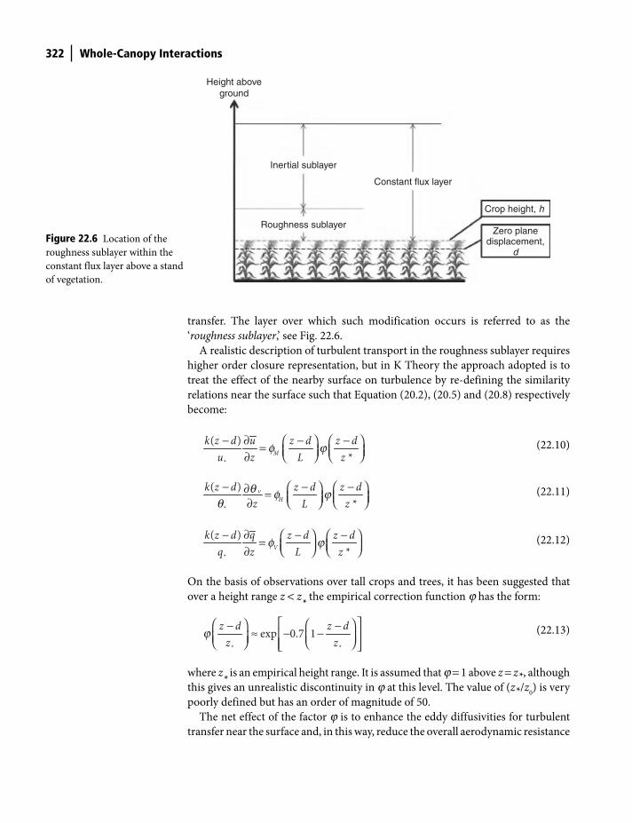
322 Whole-Canopy Interactions
transfer. The layer over which such modification occurs is referred to as the
‘ roughness sublayer,’ see Fig. 22.6.
A realistic description of turbulent transport in the roughness sublayer requires
higher order closure representation, but in K Theory the approach adopted is to
treat the effect of the nearby surface on turbulence by re-defining the similarity
relations near the surface such that Equation (20.2), (20.5) and (20.8) respectively
become:
*
( )
*M
k z d u z d z du z L z− ∂ − −⎛ ⎞ ⎛ ⎞= ⎜ ⎟ ⎜ ⎟⎝ ⎠ ⎝ ⎠∂
f j (22.10)
*
( )
*v
Hk z d z d z d
z L z− − −⎛ ⎞ ⎛ ⎞∂ = ⎜ ⎟ ⎜ ⎟⎝ ⎠ ⎝ ⎠∂
q f jq
(22.11)
*
( )
*V
qk z d z d z dq z L z
∂− − −⎛ ⎞ ⎛ ⎞= ⎜ ⎟ ⎜ ⎟⎝ ⎠ ⎝ ⎠∂f j
(22.12)
On the basis of observations over tall crops and trees, it has been suggested that
over a height range z < z* the empirical correction function j has the form:
* *
exp 0.7 1z d z dz z
⎡ ⎤⎛ ⎞ ⎛ ⎞− −≈ − −⎢ ⎥⎜ ⎟ ⎜ ⎟⎝ ⎠ ⎝ ⎠⎢ ⎥⎣ ⎦
j (22.13)
where z* is an empirical height range. It is assumed that j = 1 above z = z*, although
this gives an unrealistic discontinuity in j at this level. The value of (z*/z0) is very
poorly defined but has an order of magnitude of 50.
The net effect of the factor j is to enhance the eddy diffusivities for turbulent
transfer near the surface and, in this way, reduce the overall aerodynamic resistance
Height aboveground
Inertial sublayer
Roughness sublayer
Constant flux layer
Crop height, h
Zero planedisplacement,
dFigure 22.6 Location of the
roughness sublayer within the
constant flux layer above a stand
of vegetation.
Shuttleworth_c22.indd 322Shuttleworth_c22.indd 322 11/3/2011 6:42:02 PM11/3/2011 6:42:02 PM
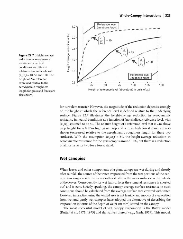
Whole-Canopy Interactions 323
for turbulent transfer. However, the magnitude of the reduction depends strongly
on the height at which the reference level is defined relative to the underlying
surface. Figure 22.7 illustrates the height-average reduction in aerodynamic
resistance in neutral conditions as a function of (normalized) reference level, with
(z*/z
0) assumed to be 50. The relative height of a reference level that is 2 m above
crop height for a 0.12 m high grass crop and a 10 m high forest stand are also
shown (expressed relative to the aerodynamic roughness length for these two
surfaces). With the assumption (z*
/z0) ≈ 50, the height-average reduction in
aerodynamic resistance for the grass crop is around 10%, but there is a reduction
of almost a factor two for a forest stand.
Wet canopies
When leaves and other components of a plant canopy are wet during and shortly
after rainfall, the source of the water evaporated from the wet portions of the can-
opy is no longer inside the leaves, rather it is from the water surfaces on the outside
of the leaves. Consequently for wet leaf surfaces the stomatal resistance is ‘shorted
out’ and is zero. Strictly speaking, the canopy average surface resistance in such
conditions should be calculated from the average surface area covered with water.
However, in practice, using the wetted area is not feasible and models of evaporation
from wet and partly wet canopies have adopted the alternative of describing the
evaporation in terms of the depth of water (in mm) stored on the canopy.
The most successful model of wet canopy evaporation is the Rutter model
(Rutter et al., 1971; 1975) and derivatives thereof (e.g., Gash, 1979). This model,
1.0
0.9
0.8
0.7
0.6
0.50 25 50 75 100 125 150
z*
z*Z0
= 10
= 50
= 100
Height of reference level [above(z-d ) in units of z0]
Hei
ght a
vera
ge r
educ
tion
fact
or
Reference level2m above forest
Reference level2m above grass
Z0
Z0
z*
Figure 22.7 Height average
reduction in aerodynamic
resistance in neutral
conditions for different
relative reference levels with
(z*/z
0) = 10, 50 and 100. The
height of 2 m reference
expressed relative to the
aerodynamic roughness
length for grass and forest are
also shown.
Shuttleworth_c22.indd 323Shuttleworth_c22.indd 323 11/3/2011 6:42:06 PM11/3/2011 6:42:06 PM
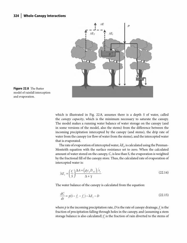
324 Whole-Canopy Interactions
which is illustrated in Fig. 22.8, assumes there is a depth S of water, called
the canopy capacity, which is the minimum necessary to saturate the canopy.
The model makes a running water balance of water storage on the canopy (and
in some versions of the model, also the stems) from the difference between the
incoming precipitation intercepted by the canopy (and stems), the drip rate of
water from the canopy (or flow of water from the stems), and the intercepted water
that is evaporated.
The rate of evaporation of intercepted water, lEI, is calculated using the Penman-
Monteith equation with the surface resistance set to zero. When the calculated
amount of water stored on the canopy, C, is less than S, the evaporation is weighted
by the fractional fill of the canopy store. Thus, the calculated rate of evaporation of
intercepted water is:
( )ρΔ +⎛ ⎞λ = ⎜ ⎟⎝ ⎠ Δ + γa p ref a
I
A c D rCES
(22.14)
The water balance of the canopy is calculated from the equation:
(1 )t s IdC p f f E Ddt
= − − − λ − (22.15)
where p is the incoming precipitation rate, D is the rate of canopy drainage, fc is the
fraction of precipitation falling through holes in the canopy, and (assuming a stem
storage balance is also calculated) fs is the fraction of rain diverted to the stems of
PlE
lEIlET
S
St
Figure 22.8 The Rutter
model of rainfall interception
and evaporation.
Shuttleworth_c22.indd 324Shuttleworth_c22.indd 324 11/3/2011 6:42:06 PM11/3/2011 6:42:06 PM
Whole-Canopy Interactions 325
the vegetation. One expression for the drainage rate that has been used in the
Rutter model is:
[ ]exp ( )D a b C S= −
(22.16)
with a = 0.002 mm min−1 and b = 4 mm being typical values. The total evaporation
from the canopy includes that from the intercepted water, lEI, and that from any
dry leaves, lET, and is estimated from the weighted sum:
1T IC CE E ES S
⎛ ⎞ ⎛ ⎞λ = λ + − λ⎜ ⎟ ⎜ ⎟⎝ ⎠ ⎝ ⎠
(22.17)
where
( )( )1
a p ref aT
s a
A c D rE
r r
Δ +λ =
Δ + +
r
g
(22.18)
where rs is the surface resistance of the canopy were it all dry.
The Rutter model of canopy interceptions has been adopted in the land surface
schemes of General Circulation Models but it has sometimes been substantially
simplified when used in this application. A running canopy water balance is
still made, but evaporation is set equal to lEI whenever C > 0, and D = 0 whenever
C < S, but D = p-S whenever p > S.
Recently there have been developments of the original Rutter model described
above to allow its use in sparse canopies (e.g., Valente et al., 1997). In essence the
approach used is to separate the landscape into two portions, a fraction c without
vegetation cover for which it is assumed there is no interception loss, and a frac-
tion (1-c) with vegetation cover for which evaporation is assumed calculated using
a version of the original Rutter model, perhaps with a simplified description of
drainage similar to that decribed in the last paragraph. This revised sparse canopy
version of the Rutter model is now accepted as being the preferred form because
as the fractional vegetation cover changes, it has appropriate asymptotic limits.
For a recent comprehensive review of models of wet canopy interception loss the
reader is referred to Muzylo et al. (2009).
Equilibrium evaporation
Consider the enclosed volume, V, of air above a water surface of area, A, inside a
thermally insulating box, shown in Fig. 22.9. Assume the air is well-mixed and has
reached saturation. Now assume that for a period δt, a radiant energy input flux,
Rn, is applied to the water surface but the air remains well-mixed. The incoming
energy will be used to both evaporate some of the water and to raise the temperature
Shuttleworth_c22.indd 325Shuttleworth_c22.indd 325 11/3/2011 6:42:09 PM11/3/2011 6:42:09 PM

326 Whole-Canopy Interactions
of the air so that it remains saturated. To do this there is a sensible heat flux, H, and
a latent heat flux, λE, from the surface to the air above.
While the air is heating and moistening over the period δt, energy conservation
requires that:
nR H E= + l
(22.19)
Over this same period, heat conservation in the air requires that the heat input
from the surface equals the change in heat stored in the air as its temperature rises
by δT, i.e., that:
( ). ( ).a pHA t V c T= ρd d
(22.20)
Mass conservation in the air also requires that the flux of moisture from the surface
is equal to the change in water vapor in the volume V, i.e. that the increase in the
specific humidity, δq, is such that:
( ) ( )aEA t V q= ρd d
(22.21)
Because δq = 0.622(δe/P), see Equation (2.9), this means:
0.622( )( ) aV eEA t
Pρ
=d
d
(22.22)
However, by definition, Δ = (δe/δT), hence:
0.622( )( ) aV TEA t
Pρ Δ
=d
d
(22.23)
Dividing Equation (22.20) by Equation (22.23), then dividing both sides of the
resulting equation by λ and identifying the psychrometric constant among the
terms gives:
Well Mixed, Saturated Air
Radiant Energy Input
Thermallyinsulating
box
H
Rn
lE
Water
Figure 22.9 Equilibrium
evaporation into a saturated
atmosphere in response to a
radiant energy input to the
evaporating surface.
Shuttleworth_c22.indd 326Shuttleworth_c22.indd 326 11/3/2011 6:42:12 PM11/3/2011 6:42:12 PM
Whole-Canopy Interactions 327
HE
=Δg
l (22.24)
Finally, combining Equations (22.19) with Equation (22.24) gives:
nE RΔ=Δ +
lg
(22.25)
This evaporation rate is called the ‘Equilibrium evaporation rate’. It is the rate of
evaporation that would occur from natural surfaces in response to incoming energy
if the overlying atmosphere was saturated and remained saturated. As such, it is a
useful concept because it defines a lower limit on natural evaporation rates. However,
in the real world, evaporation rates are higher than this because the atmosphere is
usually not saturated because water is removed aloft by precipitation.
Evaporation into an unsaturated atmosphere
Most often natural evaporation occurs during the day into an unsaturated ABL
which is partly (but not wholly) contained by a stable inversion. The surface
evaporation rate is determined by the surface resistance and aerodynamic
resistance but also by atmospheric variables (which may be measured) in the
surface layer, specifically by net radiation, VPD, wind speed, and temperature.
However, because the ABL is partly contained, the values of these atmospheric
variables are themselves influenced by the surface energy inputs, and the potential
for surface–ABL feedbacks therefore exists.
If daytime containment of the ABL were totally effective, evaporation rate
would presumably be close to the equilibrium evaporation rate. But this is not the
case. Precipitation processes (and the associated loss of water vapor and release of
latent heat aloft) mean that the air in the free atmosphere above the daytime
inversion is on average drier and (in terms of potential temperature) warmer than
that in the ABL. As discussed in Chapter 18, intermittent breakdown of the
inversion layer during the day allows some entrainment of this drier, warmer air
from the free atmosphere into the ABL, and the ABL grows as a result. Again as
discussed in Chapter 18, some of the moisture evaporated from the ground may
remain in the ABL, but most is used to moisten the incoming drier air from the
free atmosphere. As a result the change in absolute moisture content in the ABL
can be small. On the other hand, during the day the air in the ABL is warmed both
by sensible heat from the ground and by the incoming warmer air from above.
Consequently, the temperature of the ABL rises and the VPD remains finite.
Because the VPD in the ABL is finite, natural evaporation rates from moist surfaces
are greater (typically 25% greater) than the equilibrium evaporation rate.
The extent to which dry, warm air from the free atmosphere is entrained
depends on the strength of the stable inversion. The stronger the inversion the
Shuttleworth_c22.indd 327Shuttleworth_c22.indd 327 11/3/2011 6:42:17 PM11/3/2011 6:42:17 PM
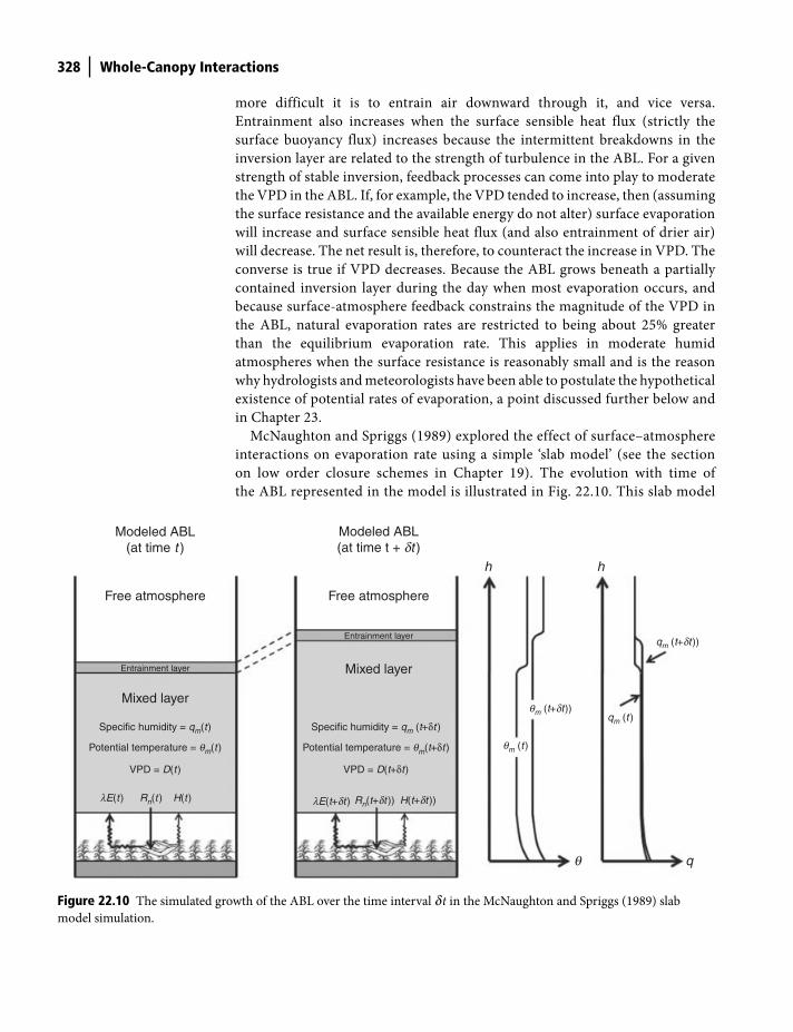
328 Whole-Canopy Interactions
more difficult it is to entrain air downward through it, and vice versa.
Entrainment also increases when the surface sensible heat flux (strictly the
surface buoyancy flux) increases because the intermittent breakdowns in the
inversion layer are related to the strength of turbulence in the ABL. For a given
strength of stable inversion, feedback processes can come into play to moderate
the VPD in the ABL. If, for example, the VPD tended to increase, then (assuming
the surface resistance and the available energy do not alter) surface evaporation
will increase and surface sensible heat flux (and also entrainment of drier air)
will decrease. The net result is, therefore, to counteract the increase in VPD. The
converse is true if VPD decreases. Because the ABL grows beneath a partially
contained inversion layer during the day when most evaporation occurs, and
because surface-atmosphere feedback constrains the magnitude of the VPD in
the ABL, natural evaporation rates are restricted to being about 25% greater
than the equilibrium evaporation rate. This applies in moderate humid
atmospheres when the surface resistance is reasonably small and is the reason
why hydrologists and meteorologists have been able to postulate the hypothetical
existence of potential rates of evaporation, a point discussed further below and
in Chapter 23.
McNaughton and Spriggs (1989) explored the effect of surface–atmosphere
interactions on evaporation rate using a simple ‘slab model’ (see the section
on low order closure schemes in Chapter 19). The evolution with time of
the ABL represented in the model is illustrated in Fig. 22.10. This slab model
Modeled ABL(at time t )
Free atmosphere
Mixed layer
Specific humidity = qm(t)
Potential temperature = qm(t )
VPD = D(t )
lE(t ) Rn(t ) H(t)
Entrainment layer
Modeled ABL(at time t + dt )
Free atmosphere
Mixed layer
Specific humidity = qm (t+δt )
Potential temperature = qm(t+δt )
VPD = D(t+δt)
lE(t+dt ) Rn(t+dt )) H(t+dt ))
Entrainment layer
h h
qm (t )
qm (t+dt))qm (t )
qm (t+dt ))
Figure 22.10 The simulated growth of the ABL over the time interval dt in the McNaughton and Spriggs (1989) slab
model simulation.
Shuttleworth_c22.indd 328Shuttleworth_c22.indd 328 11/3/2011 6:42:19 PM11/3/2011 6:42:19 PM
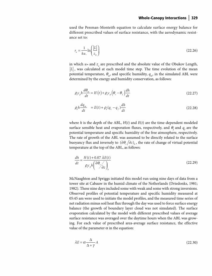
Whole-Canopy Interactions 329
used the Penman-Monteith equation to calculate surface energy balance for
different prescribed values of surface resistance, with the aerodynamic resist-
ance set to:
0*
1lna
Lr
ku z⎛ ⎞
= ⎜ ⎟⎝ ⎠
(22.26)
in which u* and zo are prescribed and the absolute value of the Obukov Length,
L , was calculated at each model time step. The time evolution of the mean
potential temperature, qm
, and specific humidity, qm
, in the simulated ABL were
determined by the energy and humidity conservation, as follows:
( ) ( )ma p a p s f
d dhc h H t cdt dt
= + −q
r r q q
(22.27)
= + −( ) ( )ma a s f
dq dhh E t q qdt dt
r r
(22.28)
where h is the depth of the ABL, H(t) and E(t) are the time-dependent modeled
surface sensible heat and evaporation fluxes, respectively, and qf and q
f are the
potential temperature and specific humidity of the free atmosphere, respectively.
The rate of growth of the ABL was assumed to be directly related to the surface
buoyancy flux and inversely to ( )v hz∂ ∂q , the rate of change of virtual potential
temperature at the top of the ABL, as follows:
( ) 0.07 ( )
va p
h
dh H t E tdt c h z
+=∂⎛ ⎞
⎜ ⎟∂⎝ ⎠
lqr
(22.29)
McNaughton and Spriggs initiated this model run using nine days of data from a
tower site at Cabauw in the humid climate of the Netherlands (Driedonks, 1981;
1982). These nine days included some with weak and some with strong inversions.
Observed profiles of potential temperature and specific humidity measured at
05:45 am were used to initiate the model profiles, and the measured time series of
net radiation minus soil heat flux through the day was used to force surface energy
balance (the growth of boundary layer cloud was not simulated). The surface
evaporation calculated by the model with different prescribed values of average
surface resistance was averaged over the daytime hours when the ABL was grow-
ing. For each value of prescribed area-average surface resistance, the effective
value of the parameter α in the equation:
E AΔ=Δ +
l ag
(22.30)
Shuttleworth_c22.indd 329Shuttleworth_c22.indd 329 11/3/2011 6:42:19 PM11/3/2011 6:42:19 PM
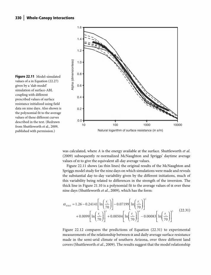
330 Whole-Canopy Interactions
was calculated, where A is the energy available at the surface. Shuttleworth et al.
(2009) subsequently re-normalized McNaughton and Spriggs’ daytime average
values of α to give the equivalent all-day average values.
Figure 22.11 shows (as thin lines) the original results of the McNaughton and
Spriggs model study for the nine days on which simulations were made and reveals
the substantial day-to-day variability given by the different initiations, much of
this variability being related to differences in the strength of the inversion. The
thick line in Figure 21.10 is a polynomial fit to the average values of α over these
nine days (Shuttleworth et al., 2009), which has the form:
2
&
3 4 5
1.26 0.24141 ln 0.07199 ln70 70
0.0099 ln 0.00504 ln 0.00083 ln70 70 70
s sM S
s s s
r r
r r r
⎡ ⎤ ⎡ ⎤⎛ ⎞ ⎛ ⎞= − −⎢ ⎥ ⎢ ⎥⎜ ⎟ ⎜ ⎟⎝ ⎠ ⎝ ⎠⎣ ⎦ ⎣ ⎦
⎡ ⎤ ⎡ ⎤ ⎡ ⎤⎛ ⎞ ⎛ ⎞ ⎛ ⎞+ + −⎢ ⎥ ⎢ ⎥ ⎢ ⎥⎜ ⎟ ⎜ ⎟ ⎜ ⎟⎝ ⎠ ⎝ ⎠ ⎝ ⎠⎣ ⎦ ⎣ ⎦ ⎣ ⎦
a
(22.31)
Figure 22.12 compares the predictions of Equation (22.31) to experimental
measurements of the relationship between α and daily average surface resistance
made in the semi-arid climate of southern Arizona, over three different land
covers (Shuttleworth et al., 2009). The results suggest that the model relationship
1.4
1.2
1.6
1.0
0.8
0.6
0.4
0.2
0.010 100 1000 10000
Natural logarithm of surface resistance (in s/m)
Alp
ha (
dim
ensi
onle
ss)
Figure 22.11 Model-simulated
values of a in Equation (22.27)
given by a ‘slab model’
simulation of surface-ABL
coupling with different
prescribed values of surface
resistance initialized using field
data on nine days. Also shown is
the polynomial fit to the average
values of these different curves
described in the text. (Redrawn
from Shuttleworth et al., 2009,
published with permission.)
Shuttleworth_c22.indd 330Shuttleworth_c22.indd 330 11/3/2011 6:42:26 PM11/3/2011 6:42:26 PM
Whole-Canopy Interactions 331
although originally developed using initiation fields taken in the humid
climate of the Netherlands may have more general applicability.
Arguably the most significant aspect of Figs 22.11 and 22.12 is that they sug-
gest that for values of surface resistance less than about 100 s m−1 (a value typical
of many unstressed natural surfaces), the ABL feedback processes described
earlier in this section seem reasonably effective at constraining the evaporation
rate to be approximately 25% greater than the equilibrium evaporation rate.
This result is broadly consistent with the proposal of Priestley and Taylor (1972)
that Equation (22.30) is an ‘appropriate framework’ for apportioning surface
1.0
0.5
0.0
1.5
10 100 1000 10000
M&S
Woodland
Surface resistance (s m−1)
(a)
α(a)
1.0
0.5
0.0
1.5M&S
Grassland
(c)
10 100 1000 10000
Surface resistance (s m−1)
α
(c)
1.0
0.5
0.0
1.5M&S
Shrubland
(b)
10 100 1000 10000
Surface resistance (s m−1)
α
(b)
Figure 22.12 Comparison between measured values of a and daily average surface resistance over (a) woodland,
(b) shrubland, and (c) grassland covers in southern Arizona, (Redrawn from Shuttleworth et al., 2009, published
with permission.)
Shuttleworth_c22.indd 331Shuttleworth_c22.indd 331 11/3/2011 6:42:27 PM11/3/2011 6:42:27 PM
332 Whole-Canopy Interactions
energy between sensible heat and evaporation, and that for ‘saturated surfaces’
a reasonable estimate of evaporation can be made from:
1.26E AΔ=
Δ +l
g (22.32)
However, Fig. 22.12 also shows that as surface resistance rises and water
availability at the surface decreases, evaporation rate necessarily falls and
ultimately becomes zero.
Important points in this chapter
● Use of in-canopy results: results from in-canopy studies of individual leaf
exchange and near-canopy turbulent transfer can improve representation of
whole canopy exchanges by single source, ‘big leaf ’ Penman-Monteith models.
● LAI dependency of aerodynamic properties: taking 0.2 as the average drag
coefficient for an individual leaf inside a canopy, Shaw and Periera (1982)
used a second order closure model of canopy exchange to give simulation
of zero plane displacement and aerodynamic roughness consistent with
field observations.
● Excess resistance: in one-dimensional models the fact that the exchange
coefficient for individual leaves is significantly less for momentum than for
other exchanges is often accommodated by assuming other exchanges act at
a source/sink deeper in the canopy and have 10 times less aerodynamic
roughness length than momentum.
● Enhanced efficiency of near surface turbulence: enhanced efficiency of
turbulent transfer near vegetation canopies has been accommodated in K
Theory by a height dependent re-definition of similarity relations and
typically reduces aerodynamic resistance for short crops by ∼10% but for tall
(forest) crops by about a factor of two.
● Rutter model: the most successful representation of evaporation from
canopies wet or partially wet during and after rain is using the Rutter model
or derivatives thereof, which make a running balance of rain water stored on
vegetation and assume evaporation of intercepted water is proportional to
the fractional fill of a canopy water store.
● Equilibrium evaporation: when incoming radiant energy is incident on a
water surface evaporating into an isolated volume of air, the energy is shared
as latent and sensible heat inputs to the air such as to keep the air saturated
and evaporation occurs at a well-defined equilibrium evaporation rate given
by Equation (22.25).
● Greater than equilibrium evaporation: evaporation mainly occurs during
the day into an ABL partly (but not wholly) constrained by a stable inversion,
Shuttleworth_c22.indd 332Shuttleworth_c22.indd 332 11/3/2011 6:42:27 PM11/3/2011 6:42:27 PM
Whole-Canopy Interactions 333
consequently the ABL usually remains unsaturated and the evaporation rate
from an underlying moist surface is therefore higher than the equilibrium
evaporation rate.
● Modeling ABL feedbacks: modeling feedback processes in a partly
constrained ABL gives an approximate relationship between land surface
evaporation rate and surface resistance that is consistent with observations
within (albeit large) experimental errors, see Fig. 22.12.
● Origin of potential evaporation hypothesis: surface-atmosphere feedbacks
constrain the magnitude of the VPD in the ABL such that for land surfaces
with fairly small surface resistance, evaporation into a humid atmosphere is
typically ∼25% greater than the equilibrium evaporation rate. The presence
of ABL feedbacks is why it has been possible for hydrologists to postulate the
hypothetical existence of potential rates of evaporation.
References
Driedonks, A.G.M. (1981) Dynamics of the well-mixed atmospheric boundary layer.
Scientific Report W.R. 81-2 K.N.M.I., De Bilt, The Netherlands.
Driedonks, A.G.M. (1982) Models and observations of the growth of the atmospheric
boundary layer. Boundary-Layer Meteorology, 23, 283–306.
Garratt, J.R. (1992) The Atmospheric Boundary Layer. Cambridge University Press,
Cambridge, UK.
Gash, J.H.C. (1979) An analytical model of rainfall interception by forests. Quarterly Journal
of the Royal Meteorological Society. 105, 43–55.
Muzylo. A., Llorens, P., Valente, F., Keizer, J. J., Domingo, F. and Gash, J.H.C. (2009)
A review of rainfall interception modeling. Journal of Hydrology, 370, 191–206.
McNaughton, K.G. and Spriggs, T.W. (1989) An evaluation of the Priestley-Taylor equation.
In Black, T.A., Spittlehouse, D.L., Novak, M.D. and Price, D.T. (eds) Estimation of Areal
Evaporation. IAHS Publication No.177, IAHS Press, Wallingford, UK.
Priestley, C.H.B. and Taylor, R.J. (1972) On the assessment of surface heat flux and evapora-
tion using large scale parameters. Monthly Weather Review, 100, 81–92.
Rutter, A.J., Kershaw, K.A., Robins, P.C. and Morton, A.J. (1971) A predictive model of
rainfall interception in forests, 1. Derivation of the model from observations in a planta-
tion of Corsican pine. Agricultural Meteorology, 9, 367–384.
Rutter, A.J., Morton, A.J. and Robins, P.C. (1975) A predictive model of rainfall interception
in forests. II. Generalization of the model and comparison with observations in some
coniferous and hardwood stands. Journal of Applied Ecology, 12 (1), 367–380.
Shaw, R.H. and Pereira, A.R. (1982) Aerodynamic roughness of a plant canopy: A numeri-
cal experiment. Agricultural Meteorology, 26, 51–65.
Shuttleworth, W.J., Serrat-Capdevila, A., Roderick, M.L. and Scott, R.L. (2009) On the
theory relating changes in area-average and pan evaporation. Quarterly Journal of the
Royal Meteorological Society, 135, 1230–1247.
Valente, F., David, J.S. and Gash, J.H.C. (1997) Modelling interception loss for two sparse
eucalypt and pine forests in central Portugal using reformulated Rutter and Gash analytic
models. Journal of Hydrology, 190, 141–162.
Shuttleworth_c22.indd 333Shuttleworth_c22.indd 333 11/3/2011 6:42:28 PM11/3/2011 6:42:28 PM
Introduction
Broadly speaking, the understanding of processes and phenomena involved in
the interaction between the (often vegetation-covered) land surface and the
atmospheric boundary layer that were discussed in previous chapters is used in
two ways. The first way is to combine this understanding in the form of computer
sub-models, which then become important components of hydrological or
meteorological models. Such sub-models are often called soil-vegetation-
atmosphere schemes (SVATS) and they are described in the next chapter. This
chapter covers a second broad application of understanding of surface-atmosphere
interactions, which is to provide daily estimates of evaporation for use in other
hydrological and agricultural applications. This use of evaporation estimates
predates the creation of SVATS and, although the methods and formulae used
have the same basic origin, the applications are generally simpler and the methods
used involve making more assumptions.
Thus, the distinction between these two applications is in part related to
complexity. However, it is more fundamentally associated with the availability of
the meteorological data needed to calculate estimates of surface-atmosphere
exchange. In the case of SVATS, the meteorological data needed are generally
readily obtainable and they are usually available for sampling intervals of an hour
or less, perhaps from automatic weather stations in the case of hydrological
models, or as a byproduct of calculations made in other model components in the
case of meteorological models. The availability of relevant meteorological data is
usually a much more problematic issue when making the simple daily estimates
of evaporation discussed in this chapter. Moreover, data limitations can affect
the likely reliability of the method adopted to make an estimate. At best, the avail-
able data is that which might be provided by a standard agro-meteorological
climate station reporting daily. Hence, the meteorological variables used to
23 Daily Estimates of Evaporation
Terrestrial Hydrometeorology, First Edition. W. James Shuttleworth.
© 2012 John Wiley & Sons, Ltd. Published 2012 by John Wiley & Sons, Ltd.
Shuttleworth_c23.indd 334Shuttleworth_c23.indd 334 11/3/2011 6:40:21 PM11/3/2011 6:40:21 PM

Daily Estimates of Evaporation 335
estimate evaporation are themselves the estimates of daily average or daily total
values that can be derived from the limited measurements taken at such climate
stations, as discussed in the next section. In many cases the recommended
approach used to estimate daily values is obvious, or versions of the equations used
have been defined earlier; to reduce the scope for misunderstanding these methods
are also given explicitly below.
Daily average values of weather variables
Temperature, humidity, and wind speed
Daily maximum and minimum air temperature, Tmax
and Tmin
, respectively, are
usually measured at climate stations. These can be used to estimate the daily
average air temperature, T, and the daily average saturated vapor pressure, es, from:
max min
2
T TT
+=
(23.1)
and:
max min( ) ( )
2sat sat
se T e Te +
=
(23.2)
where, for example, esat
(Tmax
) represents the function of Tmax
given as Equation
(2.17). Because the relationship between saturated vapor pressure and tempera-
ture is not linear, using Equation (23.2) is preferable to estimating es from e
sat(T).
A measurement of humidity may be available at least once (but often only once)
each day, perhaps in the form of a measurement of the wet bulb and dry bulb tem-
perature, Tdry
and Twet
, respectively, or as a measurement of relative humidity, RH,
or as a measurement of dew point temperature, Tdew
. If Tdry
and Twet
(in °C) are
available, e is calculated from Equation (2.24) which is here re-written in the form:
( ) *( - )sat wet dry wete e T T T= − g (23.3)
to emphasize that the effective value of the psychrometric constant required may well
not be γ = (cpP)/(0.6622λ) as used elsewhere, but rather a different empirically deter-
mined value, γ *. This is very likely the case if the wet and dry bulb thermometers are
not aspirated and the wet bulb depression is then smaller than the true value.
If RH (%) is available at a particular time (e.g., 09:00 local time) when the dry
bulb temperature is Tdry
′, the daily average value of e is best calculated from:
( )100
sat dryRHe e T⎛ ⎞= ⎜ ⎟⎝ ⎠
¢
(23.4)
Shuttleworth_c23.indd 335Shuttleworth_c23.indd 335 11/3/2011 6:40:22 PM11/3/2011 6:40:22 PM
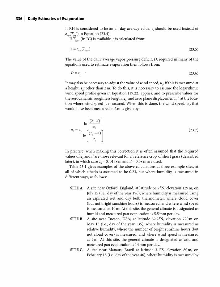
336 Daily Estimates of Evaporation
If RH is considered to be an all day average value, es should be used instead of
esat
(Tdry
′) in Equation (23.4).
If Tdew
, (in °C) is available, e is calculated from:
( )sat dewe e T= (23.5)
The value of the daily average vapor pressure deficit, D, required in many of the
equations used to estimate evaporation then follows from:
sD e e= − (23.6)
It may also be necessary to adjust the value of wind speed, uz, if this is measured at
a height, zu, other than 2 m. To do this, it is necessary to assume the logarithmic
wind speed profile given in Equation (19.22) applies, and to prescribe values for
the aerodynamic roughness length, z0, and zero plane displacement, d, at the loca-
tion where wind speed is measured. When this is done, the wind speed, u2, that
would have been measured at 2 m is given by:
0
2
0
(2 )ln
( )ln
zu
dz
u uz dz
⎡ ⎤−⎢ ⎥⎣ ⎦=⎡ ⎤−⎢ ⎥⎣ ⎦
(23.7)
In practice, when making this correction it is often assumed that the required
values of z0 and d are those relevant for a ‘reference crop’ of short grass (described
later), in which case z0 = 0. 0148 m and d = 0.08 m are used.
Table 23.1 gives examples of the above calculations at three example sites, at
all of which albedo is assumed to be 0.23, but where humidity is measured in
different ways, as follows:
SITE A A site near Oxford, England, at latitude 51.7°N, elevation 129 m, on
July 15 (i.e., day of the year 196), where humidity is measured using
an aspirated wet and dry bulb thermometer, where cloud cover
(but not bright sunshine hours) is measured, and where wind speed
is measured at 10 m. At this site, the general climate is designated as
humid and measured pan evaporation is 5.5 mm per day.
SITE B A site near Tucson, USA, at latitude 32.2°N, elevation 720 m on
May 15 (i.e., day of the year 135), where humidity is measured as
relative humidity, where the number of bright sunshine hours (but
not cloud cover) is measured, and where wind speed is measured
at 2 m. At this site, the general climate is designated as arid and
measured pan evaporation is 14 mm per day.
SITE C A site near Manaus, Brazil at latitude 3.1°S, elevation 80 m, on
February 15 (i.e., day of the year 46), where humidity is measured by
Shuttleworth_c23.indd 336Shuttleworth_c23.indd 336 11/3/2011 6:40:26 PM11/3/2011 6:40:26 PM
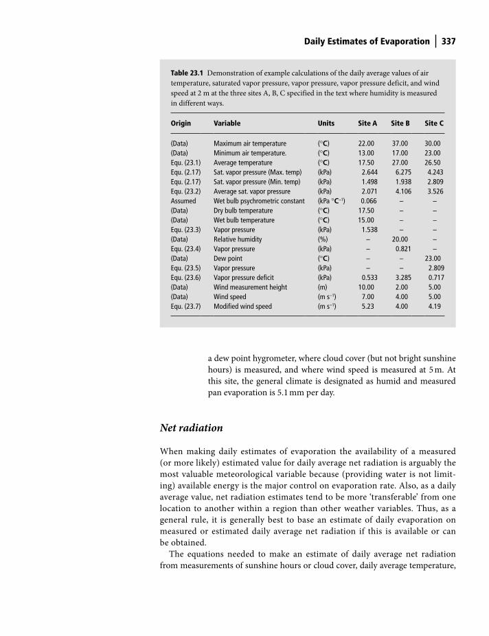
Daily Estimates of Evaporation 337
Table 23.1 Demonstration of example calculations of the daily average values of air
temperature, saturated vapor pressure, vapor pressure, vapor pressure deficit, and wind
speed at 2 m at the three sites A, B, C specified in the text where humidity is measured
in different ways.
Origin Variable Units Site A Site B Site C
(Data) Maximum air temperature (°C) 22.00 37.00 30.00(Data) Minimum air temperature. (°C) 13.00 17.00 23.00Equ. (23.1) Average temperature (°C) 17.50 27.00 26.50Equ. (2.17) Sat. vapor pressure (Max. temp) (kPa) 2.644 6.275 4.243Equ. (2.17) Sat. vapor pressure (Min. temp) (kPa) 1.498 1.938 2.809Equ. (23.2) Average sat. vapor pressure (kPa) 2.071 4.106 3.526Assumed Wet bulb psychrometric constant (kPa °C−1) 0.066 – –(Data) Dry bulb temperature (°C) 17.50 – –(Data) Wet bulb temperature (°C) 15.00 – –Equ. (23.3) Vapor pressure (kPa) 1.538 – –(Data) Relative humidity (%) – 20.00 –Equ. (23.4) Vapor pressure (kPa) – 0.821 –(Data) Dew point (°C) – – 23.00Equ. (23.5) Vapor pressure (kPa) – – 2.809Equ. (23.6) Vapor pressure deficit (kPa) 0.533 3.285 0.717(Data) Wind measurement height (m) 10.00 2.00 5.00(Data) Wind speed (m s−1) 7.00 4.00 5.00Equ. (23.7) Modified wind speed (m s−1) 5.23 4.00 4.19
a dew point hygrometer, where cloud cover (but not bright sunshine
hours) is measured, and where wind speed is measured at 5 m. At
this site, the general climate is designated as humid and measured
pan evaporation is 5.1 mm per day.
Net radiation
When making daily estimates of evaporation the availability of a measured
(or more likely) estimated value for daily average net radiation is arguably the
most valuable meteorological variable because (providing water is not limit-
ing) available energy is the major control on evaporation rate. Also, as a daily
average value, net radiation estimates tend to be more ‘transferable’ from one
location to another within a region than other weather variables. Thus, as a
general rule, it is generally best to base an estimate of daily evaporation on
measured or estimated daily average net radiation if this is available or can
be obtained.
The equations needed to make an estimate of daily average net radiation
from measurements of sunshine hours or cloud cover, daily average temperature,
Shuttleworth_c23.indd 337Shuttleworth_c23.indd 337 11/3/2011 6:40:29 PM11/3/2011 6:40:29 PM
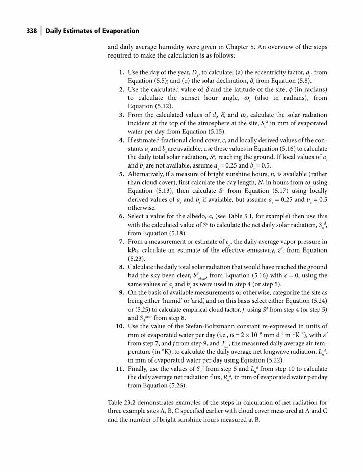
338 Daily Estimates of Evaporation
and daily average humidity were given in Chapter 5. An overview of the steps
required to make the calculation is as follows:
1. Use the day of the year, Dy, to calculate: (a) the eccentricity factor, d
r, from
Equation (5.5); and (b) the solar declination, d, from Equation (5.8).
2. Use the calculated value of d and the latitude of the site, f (in radians)
to calculate the sunset hour angle, ws (also in radians), from
Equation (5.12).
3. From the calculated values of dr, d, and w
s, calculate the solar radiation
incident at the top of the atmosphere at the site, So
d in mm of evaporated
water per day, from Equation (5.15).
4. If estimated fractional cloud cover, c, and locally derived values of the con-
stants as and b
s are available, use these values in Equation (5.16) to calculate
the daily total solar radiation, Sd, reaching the ground. If local values of as
and bs are not available, assume a
s = 0.25 and b
s = 0.5.
5. Alternatively, if a measure of bright sunshine hours, n, is available (rather
than cloud cover), first calculate the day length, N, in hours from ws using
Equation (5.13), then calculate Sd from Equation (5.17) using locally
derived values of as and b
s if available, but assume a
s = 0.25 and b
s = 0.5
otherwise.
6. Select a value for the albedo, a, (see Table 5.1, for example) then use this
with the calculated value of Sd to calculate the net daily solar radiation, Sn
d,
from Equation (5.18).
7. From a measurement or estimate of ed, the daily average vapor pressure in
kPa, calculate an estimate of the effective emissivity, e’, from Equation
(5.23).
8. Calculate the daily total solar radiation that would have reached the ground
had the sky been clear, Sdclear
, from Equation (5.16) with c = 0, using the
same values of as and b
s as were used in step 4 (or step 5).
9. On the basis of available measurements or otherwise, categorize the site as
being either ‘humid’ or ‘arid’, and on this basis select either Equation (5.24)
or (5.25) to calculate empirical cloud factor, f, using Sd from step 4 (or step 5)
and Sd
clear from step 8.
10. Use the value of the Stefan-Boltzmann constant re-expressed in units of
mm of evaporated water per day (i.e., σ = 2 × 10⁻⁹ mm d−1 m−2 K−4), with e’
from step 7, and f from step 9, and Tair
, the measured daily average air tem-
perature (in °K), to calculate the daily average net longwave radiation, Ln
d,
in mm of evaporated water per day using Equation (5.22).
11. Finally, use the values of Sn
d from step 5 and Ln
d from step 10 to calculate
the daily average net radiation flux, Rn
d, in mm of evaporated water per day
from Equation (5.26).
Table 23.2 demonstrates examples of the steps in calculation of net radiation for
three example sites A, B, C specified earlier with cloud cover measured at A and C
and the number of bright sunshine hours measured at B.
Shuttleworth_c23.indd 338Shuttleworth_c23.indd 338 11/3/2011 6:40:29 PM11/3/2011 6:40:29 PM
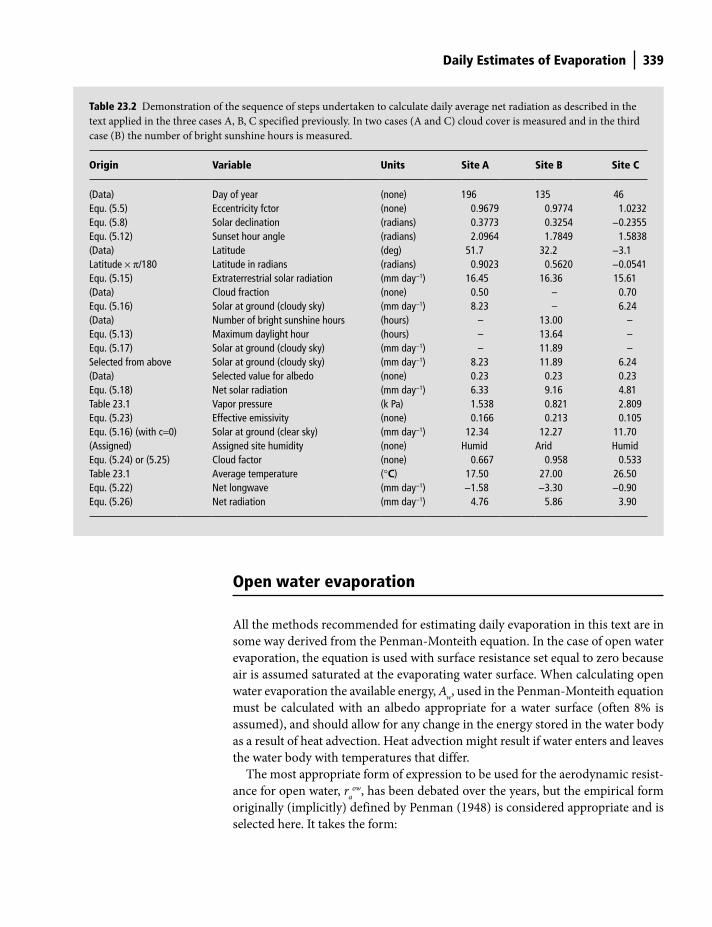
Daily Estimates of Evaporation 339
Table 23.2 Demonstration of the sequence of steps undertaken to calculate daily average net radiation as described in the
text applied in the three cases A, B, C specified previously. In two cases (A and C) cloud cover is measured and in the third
case (B) the number of bright sunshine hours is measured.
Origin Variable Units Site A Site B Site C
(Data) Day of year (none) 196 135 46Equ. (5.5) Eccentricity fctor (none) 0.9679 0.9774 1.0232Equ. (5.8) Solar declination (radians) 0.3773 0.3254 −0.2355Equ. (5.12) Sunset hour angle (radians) 2.0964 1.7849 1.5838(Data) Latitude (deg) 51.7 32.2 −3.1Latitude × π/180 Latitude in radians (radians) 0.9023 0.5620 −0.0541Equ. (5.15) Extraterrestrial solar radiation (mm day−1) 16.45 16.36 15.61(Data) Cloud fraction (none) 0.50 – 0.70Equ. (5.16) Solar at ground (cloudy sky) (mm day−1) 8.23 – 6.24(Data) Number of bright sunshine hours (hours) – 13.00 –Equ. (5.13) Maximum daylight hour (hours) – 13.64 –Equ. (5.17) Solar at ground (cloudy sky) (mm day−1) – 11.89 –Selected from above Solar at ground (cloudy sky) (mm day−1) 8.23 11.89 6.24(Data) Selected value for albedo (none) 0.23 0.23 0.23Equ. (5.18) Net solar radiation (mm day−1) 6.33 9.16 4.81Table 23.1 Vapor pressure (k Pa) 1.538 0.821 2.809Equ. (5.23) Effective emissivity (none) 0.166 0.213 0.105Equ. (5.16) (with c=0) Solar at ground (clear sky) (mm day−1) 12.34 12.27 11.70(Assigned) Assigned site humidity (none) Humid Arid HumidEqu. (5.24) or (5.25) Cloud factor (none) 0.667 0.958 0.533Table 23.1 Average temperature (°C) 17.50 27.00 26.50Equ. (5.22) Net longwave (mm day−1) −1.58 −3.30 −0.90Equ. (5.26) Net radiation (mm day−1) 4.76 5.86 3.90
Open water evaporation
All the methods recommended for estimating daily evaporation in this text are in
some way derived from the Penman-Monteith equation. In the case of open water
evaporation, the equation is used with surface resistance set equal to zero because
air is assumed saturated at the evaporating water surface. When calculating open
water evaporation the available energy, Aw, used in the Penman-Monteith equation
must be calculated with an albedo appropriate for a water surface (often 8% is
assumed), and should allow for any change in the energy stored in the water body
as a result of heat advection. Heat advection might result if water enters and leaves
the water body with temperatures that differ.
The most appropriate form of expression to be used for the aerodynamic resist-
ance for open water, ra
ow, has been debated over the years, but the empirical form
originally (implicitly) defined by Penman (1948) is considered appropriate and is
selected here. It takes the form:
Shuttleworth_c23.indd 339Shuttleworth_c23.indd 339 11/3/2011 6:40:29 PM11/3/2011 6:40:29 PM
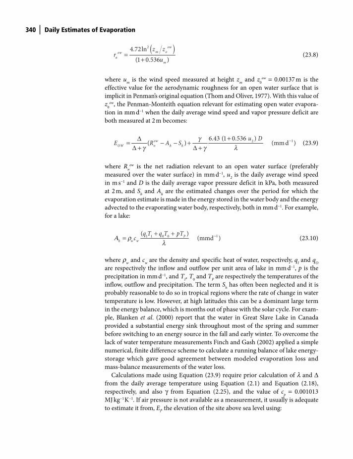
340 Daily Estimates of Evaporation
( )24.72ln
(1 0.536 )
owm oow
am
z zr
u=
+
(23.8)
where um
is the wind speed measured at height zm
and z0
ow = 0.00137 m is the
effective value for the aerodynamic roughness for an open water surface that is
implicit in Penman’s original equation (Thom and Oliver, 1977). With this value of
z0
ow, the Penman-Monteith equation relevant for estimating open water evapora-
tion in mm d−1 when the daily average wind speed and vapor pressure deficit are
both measured at 2 m becomes:
126.43 (1 0.536 )
( ) (mm d )owOW n h h
u DE R A S −+Δ
= − − +Δ + Δ +
gg g l
(23.9)
where Rn
ow is the net radiation relevant to an open water surface (preferably
measured over the water surface) in mm d−1, u2 is the daily average wind speed
in m s−1 and D is the daily average vapor pressure deficit in kPa, both measured
at 2 m, and Sh and A
h are the estimated changes over the period for which the
evaporation estimate is made in the energy stored in the water body and the energy
advected to the evaporating water body, respectively, both in mm d−1. For example,
for a lake:
−+ += 11 1 0 0
( ) (mmd )P
h w w
q T q T pTcA r
l (23.10)
where rw and c
w are the density and specific heat of water, respectively, q
I and q
O
are respectively the inflow and outflow per unit area of lake in mm d−1, p is the
precipitation in mm d−1, and TI, T
0 and T
P are respectively the temperatures of the
inflow, outflow and precipitation. The term Sh has often been neglected and it is
probably reasonable to do so in tropical regions where the rate of change in water
temperature is low. However, at high latitudes this can be a dominant large term
in the energy balance, which is months out of phase with the solar cycle. For exam-
ple, Blanken et al. (2000) report that the water in Great Slave Lake in Canada
provided a substantial energy sink throughout most of the spring and summer
before switching to an energy source in the fall and early winter. To overcome the
lack of water temperature measurements Finch and Gash (2002) applied a simple
numerical, finite difference scheme to calculate a running balance of lake energy-
storage which gave good agreement between modeled evaporation loss and
mass-balance measurements of the water loss.
Calculations made using Equation (23.9) require prior calculation of l and Δ
from the daily average temperature using Equation (2.1) and Equation (2.18),
respectively, and also γ from Equation (2.25), and the value of cp = 0.001013
MJ kg−1 K−1. If air pressure is not available as a measurement, it usually is adequate
to estimate it from, El, the elevation of the site above sea level using:
Shuttleworth_c23.indd 340Shuttleworth_c23.indd 340 11/3/2011 6:40:29 PM11/3/2011 6:40:29 PM
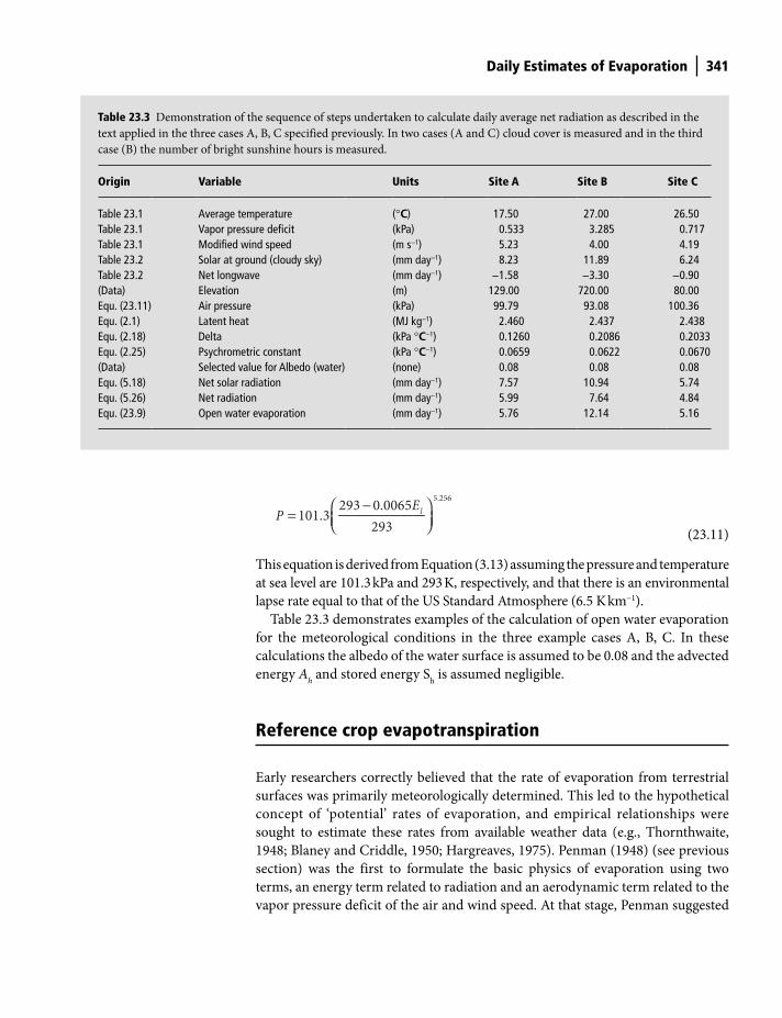
Daily Estimates of Evaporation 341
5.256293 0.0065
101.3293
lEP−⎛ ⎞
= ⎜ ⎟⎝ ⎠ (23.11)
This equation is derived from Equation (3.13) assuming the pressure and temperature
at sea level are 101.3 kPa and 293 K, respectively, and that there is an environmental
lapse rate equal to that of the US Standard Atmosphere (6.5 K km−1).
Table 23.3 demonstrates examples of the calculation of open water evaporation
for the meteorological conditions in the three example cases A, B, C. In these
calculations the albedo of the water surface is assumed to be 0.08 and the advected
energy Ah and stored energy S
h is assumed negligible.
Reference crop evapotranspiration
Early researchers correctly believed that the rate of evaporation from terrestrial
surfaces was primarily meteorologically determined. This led to the hypothetical
concept of ‘potential’ rates of evaporation, and empirical relationships were
sought to estimate these rates from available weather data (e.g., Thornthwaite,
1948; Blaney and Criddle, 1950; Hargreaves, 1975). Penman (1948) (see previous
section) was the first to formulate the basic physics of evaporation using two
terms, an energy term related to radiation and an aerodynamic term related to the
vapor pressure deficit of the air and wind speed. At that stage, Penman suggested
Table 23.3 Demonstration of the sequence of steps undertaken to calculate daily average net radiation as described in the
text applied in the three cases A, B, C specified previously. In two cases (A and C) cloud cover is measured and in the third
case (B) the number of bright sunshine hours is measured.
Origin Variable Units Site A Site B Site C
Table 23.1 Average temperature (°C) 17.50 27.00 26.50Table 23.1 Vapor pressure deficit (kPa) 0.533 3.285 0.717Table 23.1 Modified wind speed (m s−1) 5.23 4.00 4.19Table 23.2 Solar at ground (cloudy sky) (mm day−1) 8.23 11.89 6.24Table 23.2 Net longwave (mm day−1) −1.58 −3.30 −0.90(Data) Elevation (m) 129.00 720.00 80.00Equ. (23.11) Air pressure (kPa) 99.79 93.08 100.36Equ. (2.1) Latent heat (MJ kg−1) 2.460 2.437 2.438Equ. (2.18) Delta (kPa °C−1) 0.1260 0.2086 0.2033Equ. (2.25) Psychrometric constant (kPa °C−1) 0.0659 0.0622 0.0670(Data) Selected value for Albedo (water) (none) 0.08 0.08 0.08Equ. (5.18) Net solar radiation (mm day−1) 7.57 10.94 5.74Equ. (5.26) Net radiation (mm day−1) 5.99 7.64 4.84Equ. (23.9) Open water evaporation (mm day−1) 5.76 12.14 5.16
Shuttleworth_c23.indd 341Shuttleworth_c23.indd 341 11/3/2011 6:40:32 PM11/3/2011 6:40:32 PM

342 Daily Estimates of Evaporation
the potential rates of evaporation for well-watered grass and moist bare soil might
be related to that from open water using multiplicative factors.
By the mid-1970s this by then long-established way of thinking about the evaporation
process determined the United Nations’ Food and Agriculture Organization (FAO)
recommended method for estimating the water requirements for irrigated crops
(Doorenbos and Pruitt, 1977), i.e., vegetation for which stomatal resistance is not
subject to water stress. FAO followed Penman’s approach by first defining a potential
rate called ‘reference crop evapotranspiration’, ETRC
, which was defined to be the evapo-
transpiration rate for short green grass plentifully supplied with water. This rate, it was
recommended, was to be estimated by one of several alternative equations depending
on available weather data. Evapotranspiration from any other well-watered crop, ETc,
was then assumed to be calculated using a crop specific coefficient, Kc, thus:
C C RCET K ET= (23.12)
FAO provided a table of Kc values for a range of well-watered vegetation stands the
values of which (although not individually traceable by reference) are assumed
to have been derived from field studies where the well-watered crop evapotran-
spiration rate ETc and the weather variables needed to calculate ET
0 were also
measured, so that Kc could be derived. Many years of application followed and
refinements to this approach were introduced, including experiments to evaluate
and/or validate Kc for different crops in different climates (e.g., Howell et al., 2002;
Inman-Bamber and McGlinchey, 2003; Barton and Meyer, 2008).
However, the agricultural community’s adoption of the original Penman (1948)
approach as recommended by FAO failed to recognize important subsequent advances
in the specification of evapotranspiration. Penman (1963) himself determined that the
‘two stage process’ using the ‘factor’ approach wasn’t needed, and computed ‘potential
evaporation’ from any natural surface using an aerodynamic term and an energy term
specific to that surface. Shortly afterwards, Monteith generalized Penman’s ‘one step’
approach and derived the Penman-Monteith equation (introduced in Chapter 21).
Notwithstanding the publication and widespread adoption of the Penman-Monteith
equation, agriculturalists continued to use the original two-step approach. But there
were signs that the approach might be problematic when Kc values derived in one
place were used for the same crop in another place with different weather conditions.
The reason for this was demonstrated by Wallace (1995) who showed that crop
coefficients are inherently a complex mixture of both the physiology of the crop they
represent and the climate within which Kc values are derived and/or used. They also
depend on the method used to calculate reference crop evaporation.
Penman-Monteith equation estimation of ERC
With this last point in mind, and recognizing the greater realism of the
Penman-Monteith equation, FAO subsequently modified their guidelines (Allen
et al., 1998) by adopting the Penman-Monteith equation to calculate reference
Shuttleworth_c23.indd 342Shuttleworth_c23.indd 342 11/3/2011 6:40:33 PM11/3/2011 6:40:33 PM
Daily Estimates of Evaporation 343
crop evapotranspiration (ET0). However, this required retention of the two step
approach because it was still necessary to multiply ET0 by the relevant crop
coefficient to obtain actual evapotranspiration (ETc). Later in this chapter a recent
approach for estimating daily average evaporation is described that is more realis-
tic because it uses the Penman-Monteith equation to calculate estimates using
crop-specific values for unstressed surface resistance, and an aerodynamic
resistance that reflects the height of the crop. However, the FAO crop factor
method currently remains in widespread use.
The FAO definition of reference crop evaporation rate is the standard
Penman-Monteith equation used to calculate a daily average evaporation rate
assuming a specific value of surface resistance and a specific expression for
aerodynamic resistance. On the basis of field calibrations for short, well-watered
grass, rs is set equal to 70 s m−1 in Equation (21.33), while r
a (which is assumed the
same for both latent and sensible heat transfer) is calculated from Equation (22.8),
assuming the wind speed, temperature, and specific humidity and therefore, by
implication, vapor pressure deficit are all measured 2 m above 0.12 m high grass.
On the basis of field studies, the zero plane displacement, d, and aerodynamic
roughness, zo, for the grass crop are assumed given by:
0.123oz h= (23.13)
and
0.67d h= (23.14)
where h is the height of the grass crop. Substituting these values into Equation
(22.8) gives ra = 208/u
2. With these assumptions, the short grass crop-specific
version of the Penman-Monteith equation that can be used to estimate reference
crop evaporation, ERC
, in mm d−1 is:
2 2
2
900
275RC
m m
E A u DT
⎛ ⎞ ⎛ ⎞ ⎛ ⎞Δ= +⎜ ⎟ ⎜ ⎟ ⎜ ⎟Δ + Δ + +⎝ ⎠⎝ ⎠ ⎝ ⎠g
g g
(23.15)
where A is the energy available to evaporate water in mm d−1, T2, u
2, D
2 are respec-
tively the temperature in °C, wind speed in m s−1, and vapor pressure deficit in kPa
measured at 2 m, and gm is the ‘modified psychrometric constant’ which is given by;
2(1 0.33 )m u= +g g
(23.16)
Commonly A = (Rn – G), where R
n is the net radiation and G is the soil heat flux
both in mm d−1 for the short grass crop.
Equation (23.15) is strongly recommended as the preferred method for
estimating reference crop evaporation whenever daily average values of all the
required weather variables are on hand. But sometimes not all the required varia-
bles are available, and less reliable estimates of ERC
then have to be made which are
described in the next sections.
Shuttleworth_c23.indd 343Shuttleworth_c23.indd 343 11/3/2011 6:40:34 PM11/3/2011 6:40:34 PM
344 Daily Estimates of Evaporation
Radiation-based estimation of ERC
As previously stated, when estimating evaporation rates, it is recommended that
the starting point should be a measurement or estimate of the energy available to
support evaporation; because this has a strong influence on evaporation rate
when water is not limiting. Equation (22.30) can be calculated if a measurement
of the available energy (Rn-G), and temperature and pressure are available.
Temperature is needed to calculate Δ from Equation (2.18), and pressure is also
needed to calculate γ from Equation (2.25). As Fig. 22.11 shows, for a range of
surface resistances around 70 s m−1, the value of surface resistance selected for the
reference crop, Equation (22.30) can provide a reasonable estimate of evaporation
with α = 1.26.
However, it is important to recognize that this result only applies if there is
surface-ABL coupling over an extensive area with a similar surface resistance.
It could be that the area of reference crop for which an estimate of evaporation
is sought is not extensive. It could be a limited area of irrigated reference crop in
an otherwise arid landscape, for example. Therefore, some means of quantify-
ing the aridity of the advected atmosphere is required. In this context, it is
relevant that the Penman-Monteith equation (Equation (21.33) can be
re-written in the form:
lim
( )a c
a s
r rE Ar r
+= Δ
Δ + +l
g g (23.17)
where rclim
is the climatological resistance which is defined by:
2
lim (if is in W m )
a pc
c Dr A
A−⎛ ⎞
= ⎜ ⎟Δ⎝ ⎠
r
(23.18)
or:
( )1
lim
187219 187219 (if is in mm d )
(275 )1 0.622 (273.15 )c CC
D Dr AT AA e P T
−⎛ ⎞= ≈ ⎜ ⎟⎝ ⎠+ ΔΔ + +g g
(23.19)
The value of rclim
provides a measure of the relative influence of the (advected)
vapor pressure deficit and available energy on reference crop evaporation rate.
Equating the estimated evaporation rates given by Equations (22.30) and
(23.15), rearranging, and substituting rs = 70 s m−1 and r
a = 208/u
2 gives a
effective, the
value of α required to give a good estimate of reference crop evaporation, thus:
2 lim
2
( ) (208 / )
( )(208 / ) 70
ceffective
u ru
Δ + +⎡ ⎤⎣ ⎦=Δ + +
ga
g g
(23.20)
Shuttleworth_c23.indd 344Shuttleworth_c23.indd 344 11/3/2011 6:40:38 PM11/3/2011 6:40:38 PM
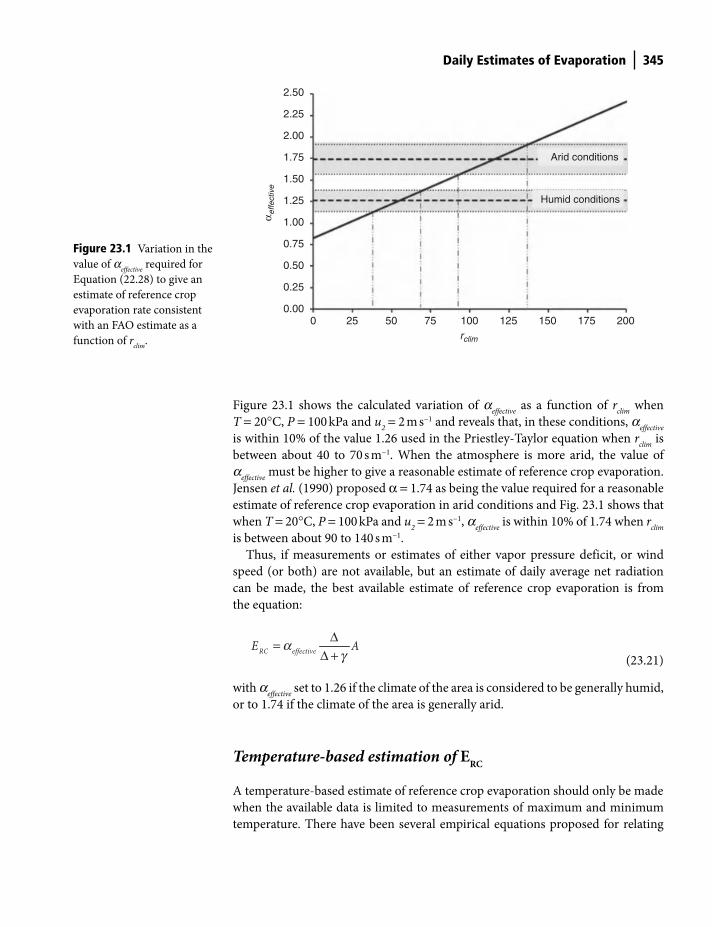
Daily Estimates of Evaporation 345
Figure 23.1 shows the calculated variation of aeffective
as a function of rclim
when
T = 20°C, P = 100 kPa and u2 = 2 m s−1 and reveals that, in these conditions, a
effective
is within 10% of the value 1.26 used in the Priestley-Taylor equation when rclim
is
between about 40 to 70 s m−1. When the atmosphere is more arid, the value of
aeffective
must be higher to give a reasonable estimate of reference crop evaporation.
Jensen et al. (1990) proposed α = 1.74 as being the value required for a reasonable
estimate of reference crop evaporation in arid conditions and Fig. 23.1 shows that
when T = 20°C, P = 100 kPa and u2 = 2 m s−1, a
effective is within 10% of 1.74 when r
clim
is between about 90 to 140 s m−1.
Thus, if measurements or estimates of either vapor pressure deficit, or wind
speed (or both) are not available, but an estimate of daily average net radiation
can be made, the best available estimate of reference crop evaporation is from
the equation:
RC effectiveE AΔ=Δ +
ag (23.21)
with aeffective
set to 1.26 if the climate of the area is considered to be generally humid,
or to 1.74 if the climate of the area is generally arid.
Temperature-based estimation of ERC
A temperature-based estimate of reference crop evaporation should only be made
when the available data is limited to measurements of maximum and minimum
temperature. There have been several empirical equations proposed for relating
2.50
2.25
2.00
1.75
1.50
1.25
1.00
0.75
0.50
0.25
0.000 25 50 75 100
rclim
125 150 175 200
α effective
Humid conditions
Arid conditions
Figure 23.1 Variation in the
value of aeffective
required for
Equation (22.28) to give an
estimate of reference crop
evaporation rate consistent
with an FAO estimate as a
function of rclim
.
Shuttleworth_c23.indd 345Shuttleworth_c23.indd 345 11/3/2011 6:40:41 PM11/3/2011 6:40:41 PM
346 Daily Estimates of Evaporation
ERC
to temperature but here the Hargreaves equation (Hargreaves, 1975) is
recommended on the grounds that its performance is at least as good as alternatives
and it is simple to use. However, the estimate given by this equation is only rele-
vant for monthly average estimates of reference crop evaporation at humid sites.
The Hargreaves equation has the form:
0.5 0.0023 ( ) ( 17.8)dRC T oE S T≈ +d
(23.22)
where So
d is the solar radiation incident at the top of the atmosphere in mm of
evaporated water per day, dT is the difference between mean monthly maximum
temperature (Tmax
) and mean monthly minimum temperature (Tmin
) in °C, and
T is the temperature in °C. Arguably the predictive ability of this empirical
equation is based on the fact that it bears some relationship to Equation (23.21).
The temperature variation of the term (T+17.8) approximates that of Δ/(Δ+γ),
the equation has an explicit link to maximum solar radiation via So
d, and through
dT, it also includes some implicit measure of the extent to which the radiation
at the top of the atmosphere reaches the surface to warm the atmosphere near
the ground.
Evaporation pan-based estimation of ERC
The measurement of weather variables requires the use of fairly expensive sensors.
For this reason evaporation pans (see Chapter 7) were often preferred in many
agricultural applications, and many pans remain in operation today (see
Chapter 7). The required estimate of reference crop evaporation is assumed to be
directly related to the measured rate of evaporation from the evaporation pan
using an equation similar to Equation (23.12), thus:
RC p panET K ET=
(23.23)
The ‘constant’ in this equation is called a ‘pan factor’. In the past the value of the
pan factor has been defined empirically by comparing reference crop evaporation
rate, lErc, with measured pan evaporation rate, lE
pan, at one location and in one
climate, and then applying this ratio elsewhere. On this basis approximate values
of pan factor were tabulated in different weather conditions (e.g. Doorenbos and
Pruitt, 1977; Shuttleworth, 1993), but such tabulation was made without proper
theoretical understanding of the origins of such variations.
In recent years there has been research into the physics that controls evapora-
tion from the Class A evaporation pan. Rotstayn et al. (2006) developed the
‘Penpan’ equation which is based on the work of Thom et al. (1981) and Linacre
(1994), and which is a physically-based description of pan evaporation in terms
of ambient climate variables. The Penpan equation is an implementation of the
Penman-Monteith equation in which the effective aerodynamic resistance for a
Class A evaporation pan is prescribed to be:
Shuttleworth_c23.indd 346Shuttleworth_c23.indd 346 11/3/2011 6:40:43 PM11/3/2011 6:40:43 PM
Daily Estimates of Evaporation 347
2
( )1 1.35
pa pan
Cr
u=
+
(23.24)
where u2 is the wind speed (in m s−1) measured at 2 m, C
p has units of s m−1 and the
factor 1.35 (implicitly) has units of s m−1. Rotstayn et al. (2006) prescribed the
effective value of surface resistance for a Class A evaporation pan when evapora-
tion is calculated using the Penman-Monteith Equation as:
( ) 1.4( )s pan a panr r=
(23.25)
with the albedo of the pan set to 14%. Roderick et al. (2007) experimentally verified
the Penman equation against Class A pan data from pan sites in Australia where the
measured meteorological variables required in the equation were also available.
They showed that, on average, the equation gave a reasonable description of
monthly-average measured pan evaporation rate, albeit with systematic site-to-site
discrepancies in the order of 10–20% when Cp is set to an average value 224 s m−1.
Thus, both the Penpan equation and FAO’s recommended equation for
calculating reference crop are implementations of the Penman-Monteith equation
with different values of aerodynamic and surface resistance, i.e., (208/u2) and 70
for a reference crop and (ra)
pan = C
p/(1+ 1.35u
2) and (r
s)
pan = 1.4r
a for a pan, respec-
tively. By substituting these pairs of values into Equation (23.23) and taking the
ratio of the two calculated rates, it follows that:
[ ]2lim 2
2 lim 2
( 2.4 ) / (1 1.35 )[ 208/ ]
70 ( )208/ ( / ) / (1 1.35 )
pcp
c p pan rc
C ur uK
u r C A A u
⎡ ⎤Δ + ++ ⎣ ⎦=+ Δ + ⎡ ⎤+ +⎣ ⎦
g
g g
(23.26)
where (Apan
/Arc) is the ratio of the energy available to support evaporation from a
reference crop to that available for an evaporation pan. Shuttleworth (2010) dem-
onstrated that the value of Kp is estimated to within an accuracy of a few percent
by setting (Apan
/Arc) = 1.15 for a wide range of short wave and longwave radiation
values, and recommended that in the absence of better information the value of
rclim
in Equation (23.26) should be calculated from:
[ ]2
clim
2
(1 0.377 )2081
ur
u⎛ ⎞Δ + +
= −⎜ ⎟Δ +⎝ ⎠
a gg
(23.27)
where u2, the wind speed measured at 2 m, is in m s−1 and with α set to 1.26 and
1.74 at humid and arid sites, respectively. Shuttleworth also showed that the value
of Kp has limited sensitivity to temperature (via the value of Δ), but has a strong
sensitivity to wind speed. In the absence of measurements, he recommended that
a default temperature of 20°C and default wind speed of 2 m s−1 are used in
Equation (23.26). When the temperature is 20°C and pressure is 100 kPa, in humid
conditions Kp has the wind speed dependent form:
Shuttleworth_c23.indd 347Shuttleworth_c23.indd 347 11/3/2011 6:40:45 PM11/3/2011 6:40:45 PM
348 Daily Estimates of Evaporation
22
2 2
0.303 / (1 1.35 )[58+208/ ]
[4.63 43.8/ ] 58 1.15 / (1 1.35 )
pp
p
C uuK
u C u
⎡ ⎤+⎣ ⎦=+ ⎡ ⎤+ +⎣ ⎦ (23.28)
while in arid conditions, it has the form:
22
2 2
0.303 / (1 1.35 )[120+208/ ]
[4.63 43.8/ ] 120 1.15 / (1 1.35 )
pp
p
C uuKu C u
⎡ ⎤+⎣ ⎦=+ ⎡ ⎤+ +⎣ ⎦ (23.29)
The implicit dimensions of the constants that appear in Equations (23.28) and
(23.29) require that Cp in s m−1 and u
2 in m s−1. Assuming C
p is the average value
224 s m−1 found by Roderick et al. (2007), then, when u2 = 2 m s−1, the default values
of Kp are 0.88 and 0.82 in humid and arid conditions, respectively. Were a calibration
of Cpan
at the pan site to be made (perhaps by temporarily deploying the sensors
needed to gather the weather data required by the Penpan equation), then the
subsequently sustained collection of wind speed measurement would give improved
accuracy for pan-based estimates of reference crop evaporation at the site.
Table 23.4 demonstrates example calculations of reference crop evaporation using
the Penman-Monteith-based FAO method and the less reliable radiation-based,
temperature-based and pan-based estimates described above for the three example
sites A, B, C. In the case of the radiation-based estimate, the value is calculated using
the most appropriate value, either 1.26 or 1.74, in Equation (23.21) depending on
whether the site is considered to have a generally humid or generally arid climate.
At the sites with humid climates A and C (sites near Oxford, England and Manaus,
Brazil), the radiation-based and temperature-based estimates of reference crop
evaporation give values that are roughly comparable to those given using the FAO
method. However, at site B near Tucson, Arizona, the radiation-based and tempera-
ture-based methods both give estimates of ERC
which are much lower than the values
given when using the FAO method, despite the fact that aeffective
= 1.74 is selected
when making the radiation-based estimate of ERC
. Pan-based estimates are made
both using relevant default values of Kp and relevant wind speed dependent estimates,
i.e., using Equation (23.27) to calculate rclim
in humid and arid conditions as
appropriate, then calculating a wind-corrected value of Kp from Equation (23.26).
The default values of Kp give overestimates because in each case the wind speed is
significantly greater than 2 m s−1.
Evaporation from unstressed vegetation: the Matt-Shuttleworth approach
Daily estimates of evaporation from vegetation cover that is plentifully supplied
with water are still usually made using Equation (23.12) with assumed values for
KC, taken from the tables provided by FAO (Allen et al., 1998) for irrigated crops.
Shuttleworth_c23.indd 348Shuttleworth_c23.indd 348 11/3/2011 6:40:49 PM11/3/2011 6:40:49 PM
Daily Estimates of Evaporation 349
Table 23.4 Demonstration of the calculation of reference crop evaporation using the FAO, radiation-based, and
temperature-based methods as described in the text for the three cases A, B, C specified previously.
Origin Variable Units Site A Site B Site C
Table 23.1 Maximum air temperature (°C) 22.00 37.00 30.00Table 23.1 Minimum air temperature (°C) 13.00 17.00 23.00Table 23.1 Average temperature (°C) 17.50 27.00 26.50Table 23.1 Vapor pressure deficit (kPa) 0.533 3.285 0.717Table 23.1 Modified wind speed (m s−1) 5.23 4.00 4.19Table 23.2 Extraterrestrial solar radiation (mm day−1) 16.45 16.36 15.61Table 23.2 Net radiation (mm day−1) 4.76 5.86 3.90Table 23.2 Assigned site humidity (none) Humid Arid HumidTable 23.3 Latent heat (MJ kg−1) 2.460 2.437 2.438Table 23.3 Delta (kPa °C−1) 0.1260 0.2086 0.2033Table 23.3 Psychrometric constant (kPa °C−1) 0.0659 0.0622 0.0670Data Measured pan evaportion (mm) 5.5 14 5.1Assumed Value of Cp in Equ. (23.24) (s m−1) 224 224 224Assumed Value of (Apan/Arc) (none) 1.15 1.15 1.15Equ. (23.16) Modified psychrometric constant (kPa °C−1) 0.1797 0.1443 0.1597Equ. (23.27) rclim assigned in Equ. (23.26) (s m−1) 44 70 37Selected Default pan coefficient (none) 0.88 0.82 0.88Equ (23.26) Wind corrected pan factor (none) 0.71 0.75 0.77Equ. (23.15) Ref. crop evap. (FAO) (mm day−1) 3.81 10.36 3.84Equ. (23.21) Ref. crop evap. (radiation based) (mm day−1) 3.94 7.85 3.70Equ. (23.22) Ref. crop evap. (temperature based) (mm day−1) 4.01 7.54 4.21Equ. (23.23) Ref. crop evap. (pan: default Kp) (mm day−1) 4.84 11.48 4.49Equ. (23.23) Ref. crop evap. (pan: wind corr. Kp) (mm day−1) 3.91 10.53 3.95
Because the FAO tables provide estimates of evaporation for irrigated crops, they
describe the seasonal evolution in the value of KC in terms of four growth stages
with crop-specific duration as shown for a hypothetical crop in Fig. 23.2.
The reluctance of the agricultural irrigation community to change practice and
adopt estimates based on using the Penman-Monteith equation with crop- specific
surface resistances may partly be due to a lack of appreciation of the basic flaws in
using Equation (23.12). However, a more fundamental inhibition on change is that
specified values of aerodynamic resistance and surface resistance are required for
non-stressed, well-watered, irrigated crops. Hitherto these have not been readily
available. Shuttleworth (2006) addressed this need by combining modern thinking
in surface energy exchange and boundary layer meteorology to derive a means of:
● specifying aerodynamic resistance of any crop from readily available (2 m)
climate station data; and
● converting existing Kc values to their equivalent values of surface resistance.
Shuttleworth_c23.indd 349Shuttleworth_c23.indd 349 11/3/2011 6:40:50 PM11/3/2011 6:40:50 PM
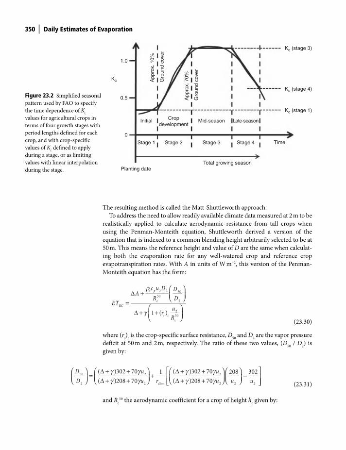
350 Daily Estimates of Evaporation
The resulting method is called the Matt-Shuttleworth approach.
To address the need to allow readily available climate data measured at 2 m to be
realistically applied to calculate aerodynamic resistance from tall crops when
using the Penman-Monteith equation, Shuttleworth derived a version of the
equation that is indexed to a common blending height arbitrarily selected to be at
50 m. This means the reference height and value of D are the same when calculat-
ing both the evaporation rate for any well-watered crop and reference crop
evapotranspiration rates. With A in units of W m−2, this version of the Penman-
Monteith equation has the form:
2 2 5050
2
250
1 ( )
a p
cRC
s cc
c u D DADR
ETurR
⎛ ⎞Δ + ⎜ ⎟⎝ ⎠
=⎛ ⎞
Δ + +⎜ ⎟⎝ ⎠
r
g (23.30)
where (rs)
c is the crop-specific surface resistance, D
50 and D
2 are the vapor pressure
deficit at 50 m and 2 m, respectively. The ratio of these two values, (D50
/ D2) is
given by:
1.0
0.5
0
Planting dateTotal growing season
TimeStage 4Stage 3Stage 2Stage 1
Late-seasonMid-seasonCropdevelopment
Initial
Kc (stage 3)
Kc (stage 4)
Kc (stage 1)
Kc App
rox.
10%
Gro
und
cove
r
App
rox.
70%
Gro
und
cove
r
Figure 23.2 Simplified seasonal
pattern used by FAO to specify
the time dependence of Kc
values for agricultural crops in
terms of four growth stages with
period lengths defined for each
crop, and with crop-specific
values of Kc defined to apply
during a stage, or as limiting
values with linear interpolation
during the stage.
50 2 2
2 2 clim 2 2 2
( )302 70 ( )302 701 208 302
( )208 70 ( )208 70
D u uD u r u u u
⎡ ⎤⎛ ⎞ ⎛ ⎞ ⎛ ⎞ ⎛ ⎞Δ + + Δ + += + −⎢ ⎥⎜ ⎟ ⎜ ⎟ ⎜ ⎟ ⎜ ⎟Δ + + Δ + +⎝ ⎠ ⎝ ⎠ ⎝ ⎠ ⎝ ⎠⎢ ⎥⎣ ⎦
g g g gg g g g
(23.31)
and Rc50 the aerodynamic coefficient for a crop of height h
c given by:
Shuttleworth_c23.indd 350Shuttleworth_c23.indd 350 11/3/2011 6:40:51 PM11/3/2011 6:40:51 PM
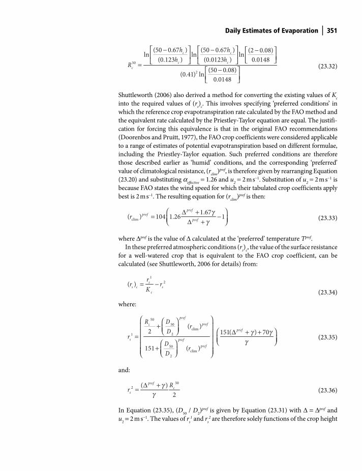
Daily Estimates of Evaporation 351
50
2
(50 0.67 ) (50 0.67 ) (2 0.08)ln ln ln
(0.123 ) (0.0123 ) 0.0148
(50 0.08)(0.41) ln
0.0148
c c
c cc
h hh h
R
⎡ ⎤ ⎡ ⎤− − −⎡ ⎤⎢ ⎥ ⎢ ⎥ ⎢ ⎥⎣ ⎦⎣ ⎦ ⎣ ⎦=
−⎡ ⎤⎢ ⎥⎣ ⎦
(23.32)
Shuttleworth (2006) also derived a method for converting the existing values of Kc
into the required values of (rs)
c. This involves specifying ‘preferred conditions’ in
which the reference crop evapotranspiration rate calculated by the FAO method and
the equivalent rate calculated by the Priestley-Taylor equation are equal. The justifi-
cation for forcing this equivalence is that in the original FAO recommendations
(Doorenbos and Pruitt, 1977), the FAO crop coefficients were considered applicable
to a range of estimates of potential evapotranspiration based on different formulae,
including the Priestley-Taylor equation. Such preferred conditions are therefore
those described earlier as ‘humid’ conditions, and the corresponding ‘preferred’
value of climatological resistance, (rclim
)pref, is therefore given by rearranging Equation
(23.20) and substituting aeffective
= 1.26 and u2 = 2 m s−1. Substitution of u
2 = 2 m s−1 is
because FAO states the wind speed for which their tabulated crop coefficients apply
best is 2 m s−1. The resulting equation for (rclim
)pref is then:
clim
1.67( ) 104 1.26 1
prefpref
prefr⎛ ⎞Δ +
= −⎜ ⎟Δ +⎝ ⎠g
g
(23.33)
where Δpref is the value of Δ calculated at the ‘preferred’ temperature Tpref.
In these preferred atmospheric conditions (rs)
c, the value of the surface resistance
for a well-watered crop that is equivalent to the FAO crop coefficient, can be
calculated (see Shuttleworth, 2006 for details) from:
1
2( ) ss c s
c
rr r
K= −
(23.34)
where:
50
50clim
21
50clim
2
( )2 151( ) 70
151 ( )
prefprefc
pref
s prefpref
R Dr
Dr
Dr
D
⎛ ⎞⎛ ⎞+⎜ ⎟⎜ ⎟ ⎛ ⎞⎝ ⎠ Δ + +⎜ ⎟= ⎜ ⎟⎜ ⎟ ⎝ ⎠⎛ ⎞⎜ ⎟+ ⎜ ⎟⎜ ⎟⎝ ⎠⎝ ⎠
g gg
(23.35)
and:
502 ( )
2
prefc
sRr Δ += g
g
(23.36)
In Equation (23.35), (D50
/ D2)pref is given by Equation (23.31) with Δ = Δpref and
u2 = 2 m s−1. The values of r
s1 and r
s2 are therefore solely functions of the crop height
Shuttleworth_c23.indd 351Shuttleworth_c23.indd 351 11/3/2011 6:40:53 PM11/3/2011 6:40:53 PM

352 Daily Estimates of Evaporation
and the temperature (known or assumed) at which the original crop coefficient Kc
was calibrated. Consequently the remaining need is to specify the value of Tpref.
Shuttleworth and Wallace (2010) investigated the sensitivity of the calculated
value of surface resistance to the assumed value of Tpref for a range of irrigated
crops in Australia and found a lack of sensitivity for many. On the basis of their
study, they concluded that, pending field studies to better define the crop-specific
values of surface resistance, Tpref = 20°C should be used in Equations (23.35) and
(22.36) when estimating (rs)
c from the tabulated values of K
c given by FAO
(Doorenbos and Pruitt, 1977). On this basis, Shuttleworth and Wallace then calcu-
lated the values of Rc50 from Equation (23.32) and (r
s)
c from Equation (23.34) for
the selection of crops given in Table 23.5.
Table 23.5 Values of crop factor, Kc, and crop height, h
c, for a selection of irrigated crops
together with the equivalent derived values of Rc50 and (rs)
c required for in Equation (12.21)
when calculating daily average evaporation using the Matt-Shuttleworth approach.
Irrigated crop Kc (dimensionless) hc (m) Rc50 (dimensionless) (rs)c (s m−1)
Reference crop 1.00 0.12 302 70Alfalfa (average) 0.95 0.70 196 127Bermuda 1.00 0.35 235 92Clover (average) 0.90 0.60 204 149Rye (average) 1.05 0.30 244 66Pasture (rotation) 0.95 0.23 260 109Pasture (extensive) 0.75 0.10 314 254Small vegetables 1.05 0.38 230 72Solanum family 1.15 0.70 196 50Cucurbitaceae 1.00 0.34 237 91Roots and tubers 1.10 0.68 198 66Legumes 1.15 0.55 209 44Cereals 1.15 1.00 177 60Cotton 1.18 1.35 162 60Maize (grain) 1.20 2.00 143 64Sorgum (grain) 1.05 1.50 157 100Rice 1.20 1.00 177 46Millet 1.00 1.50 157 118Sugar cane 1.25 3.00 124 63Cacao 1.05 3.00 124 113Coffee 0.95 2.50 133 143Tea 1.00 1.50 157 118Grape (table) 0.85 2.00 143 184Grape (wine) 0.70 1.75 149 273Almonds 0.90 5.00 102 169Avocado 0.85 3.00 124 186Citrus (50% canopy) 0.60 3.00 124 345Kiwi 1.05 3.00 124 113Walnut 1.10 4.50 107 106Olives 0.70 4.00 112 265
Shuttleworth_c23.indd 352Shuttleworth_c23.indd 352 11/3/2011 6:40:58 PM11/3/2011 6:40:58 PM

Daily Estimates of Evaporation 353
To enhance comparability with the FAO method for estimating reference crop
evaporation, Equation (23. 30) can be re-written to give crop evaporation, EC, as:
50 2 2
50
2 2
187219
* * 275C
m m c
D u DE AT D R
⎛ ⎞ ⎛ ⎞ ⎛ ⎞ ⎛ ⎞Δ= +⎜ ⎟ ⎜ ⎟ ⎜ ⎟ ⎜ ⎟Δ + Δ + +⎝ ⎠ ⎝ ⎠⎝ ⎠ ⎝ ⎠g
g g
(23.37)
where A is the energy available to evaporate water from the crop in mm d−1, T2, u
2
and D2 are respectively the temperature in °C, wind speed in m s−1, and vapor
pressure deficit in kPa measured at 2 m, and γm
* is the ‘re-modified’ psychrometric
constant, given by;
2
50
( )* 1 s c
mc
r uR
⎛ ⎞= +⎜ ⎟⎝ ⎠
g g
(23.38)
with the values of (rs)
c and R
c50 taken from tables such as Table 23.5.
Table 23.6 demonstrates example calculations of daily average evaporation from
unstressed crops calculated using the Matt-Shuttleworth approach and the FAO
crop factor method at the three example sites A, B and C specified previously, with
values of Kc, (r
s)
c and R
c50 taken from Table 23.5 for three example crops, i.e., cereal
crops, an alfalfa crop and small vegetables. These results show there are differences
between the estimated daily evaporation rates when calculated using the more real-
istic Matt-Shuttleworth approach relative to those calculated using the FAO crop
factor method. At the two humid sites, the estimated daily average evaporation rates
given by the Matt-Shuttleworth approach are slightly less than those given by the
FAO crop factor method. However, at the arid site the estimated daily average evapo-
ration rates given using the Matt-Shuttleworth approach are significantly greater
than those given by the FAO crop factor method. This is to be expected and is real-
istic: the higher evaporation rate reflects the fact that for crops with crop height
greater than the reference crop, the aerodynamic resistance is less. Consequently the
evaporation rate will necessarily be more sensitive to atmospheric aridity, in general,
and will be greater in arid conditions because the advection term in the Penman-
Monteith equation becomes more significant in comparison with the radiation term.
Evaporation from water stressed vegetation
The approach used to represent the effect of soil water restrictions on evaporation
rate which applied in conjunction with the simple models of daily average evapo-
ration described in this chapter is usually not complex. Typically, a volume of soil
is defined that is considered to be accessible to the atmosphere via plants, the
depth of which may be related to the nature of the overlying vegetation through an
assumed rooting depth. A running water balance is then made for this soil sample.
The primary input to this water balance is precipitation, and the primary output is
Shuttleworth_c23.indd 353Shuttleworth_c23.indd 353 11/3/2011 6:40:58 PM11/3/2011 6:40:58 PM
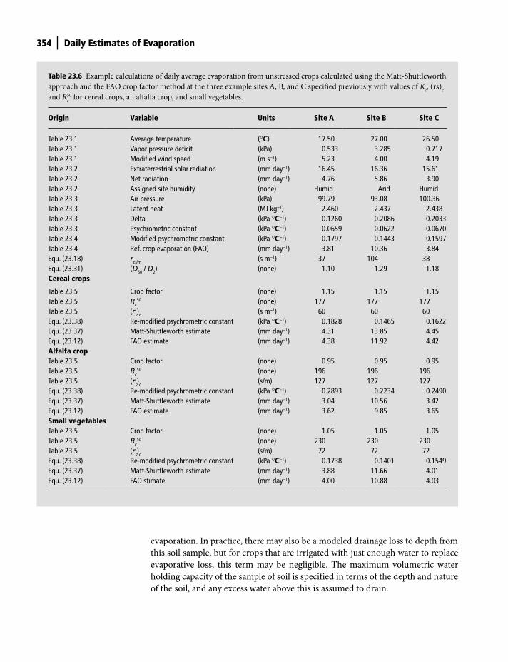
354 Daily Estimates of Evaporation
Table 23.6 Example calculations of daily average evaporation from unstressed crops calculated using the Matt-Shuttleworth
approach and the FAO crop factor method at the three example sites A, B, and C specified previously with values of Kc, (rs)
c
and Rc50 for cereal crops, an alfalfa crop, and small vegetables.
Origin Variable Units Site A Site B Site C
Table 23.1 Average temperature (°C) 17.50 27.00 26.50Table 23.1 Vapor pressure deficit (kPa) 0.533 3.285 0.717Table 23.1 Modified wind speed (m s−1) 5.23 4.00 4.19Table 23.2 Extraterrestrial solar radiation (mm day−1) 16.45 16.36 15.61Table 23.2 Net radiation (mm day−1) 4.76 5.86 3.90Table 23.2 Assigned site humidity (none) Humid Arid HumidTable 23.3 Air pressure (kPa) 99.79 93.08 100.36Table 23.3 Latent heat (MJ kg−1) 2.460 2.437 2.438Table 23.3 Delta (kPa °C−1) 0.1260 0.2086 0.2033Table 23.3 Psychrometric constant (kPa °C−1) 0.0659 0.0622 0.0670Table 23.4 Modified psychrometric constant (kPa °C−1) 0.1797 0.1443 0.1597Table 23.4 Ref. crop evaporation (FAO) (mm day−1) 3.81 10.36 3.84Equ. (23.18) rclim (s m−1) 37 104 38Equ. (23.31) (D50 / D2) (none) 1.10 1.29 1.18Cereal crops
Table 23.5 Crop factor (none) 1.15 1.15 1.15Table 23.5 Rc
50 (none) 177 177 177Table 23.5 (rs)c (s m−1) 60 60 60Equ. (23.38) Re-modified psychrometric constant (kPa °C−1) 0.1828 0.1465 0.1622Equ. (23.37) Matt-Shuttleworth estimate (mm day−1) 4.31 13.85 4.45Equ. (23.12) FAO estimate (mm day−1) 4.38 11.92 4.42Alfalfa cropTable 23.5 Crop factor (none) 0.95 0.95 0.95Table 23.5 Rc
50 (none) 196 196 196Table 23.5 (rs)c (s/m) 127 127 127Equ. (23.38) Re-modified psychrometric constant (kPa °C−1) 0.2893 0.2234 0.2490Equ. (23.37) Matt-Shuttleworth estimate (mm day−1) 3.04 10.56 3.42Equ. (23.12) FAO estimate (mm day−1) 3.62 9.85 3.65Small vegetablesTable 23.5 Crop factor (none) 1.05 1.05 1.05Table 23.5 Rc
50 (none) 230 230 230Table 23.5 (rs)c (s/m) 72 72 72Equ. (23.38) Re-modified psychrometric constant (kPa °C−1) 0.1738 0.1401 0.1549Equ. (23.37) Matt-Shuttleworth estimate (mm day−1) 3.88 11.66 4.01Equ. (23.12) FAO stimate (mm day−1) 4.00 10.88 4.03
evaporation. In practice, there may also be a modeled drainage loss to depth from
this soil sample, but for crops that are irrigated with just enough water to replace
evaporative loss, this term may be negligible. The maximum volumetric water
holding capacity of the sample of soil is specified in terms of the depth and nature
of the soil, and any excess water above this is assumed to drain.
Shuttleworth_c23.indd 354Shuttleworth_c23.indd 354 11/3/2011 6:41:00 PM11/3/2011 6:41:00 PM
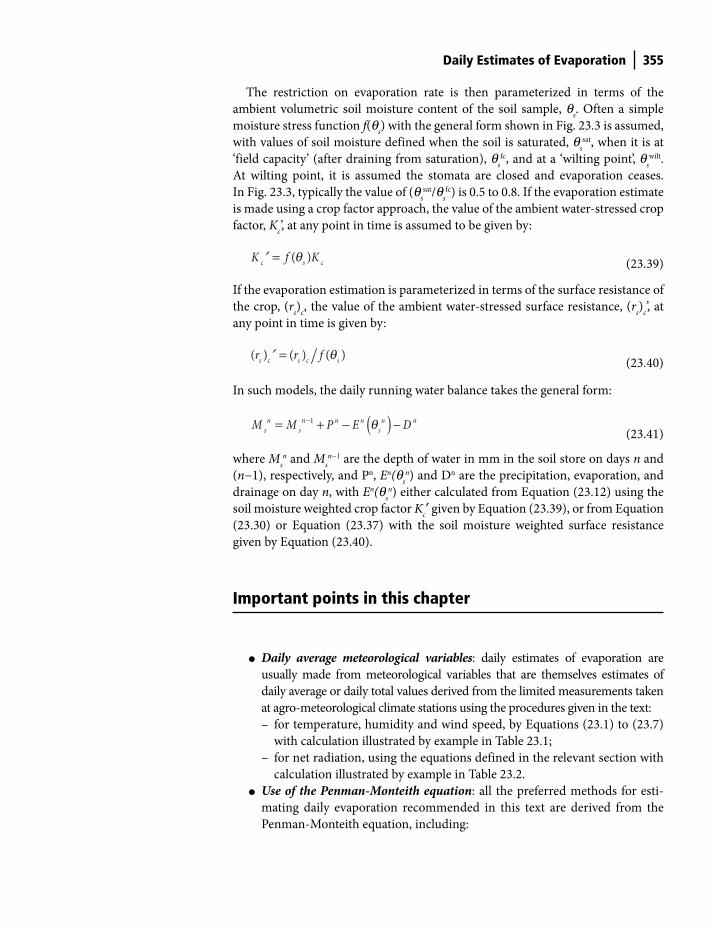
Daily Estimates of Evaporation 355
The restriction on evaporation rate is then parameterized in terms of the
ambient volumetric soil moisture content of the soil sample, qs. Often a simple
moisture stress function f(qs) with the general form shown in Fig. 23.3 is assumed,
with values of soil moisture defined when the soil is saturated, qssat, when it is at
‘field capacity’ (after draining from saturation), qsfc, and at a ‘wilting point’, q
swilt.
At wilting point, it is assumed the stomata are closed and evaporation ceases.
In Fig. 23.3, typically the value of (qssat/q
sfc) is 0.5 to 0.8. If the evaporation estimate
is made using a crop factor approach, the value of the ambient water-stressed crop
factor, Kc’, at any point in time is assumed to be given by:
( )c s cK f K=¢ q (23.39)
If the evaporation estimation is parameterized in terms of the surface resistance of
the crop, (rs)
c, the value of the ambient water-stressed surface resistance, (r
s)
c’, at
any point in time is given by:
( ) ( ) ( )s c s c sr r f=¢ q (23.40)
In such models, the daily running water balance takes the general form:
( )1n n n n n ns s sM M P E D−= + − −q
(23.41)
where Msn and M
sn−1 are the depth of water in mm in the soil store on days n and
(n−1), respectively, and Pn, En(qsn) and Dn are the precipitation, evaporation, and
drainage on day n, with En(qsn) either calculated from Equation (23.12) using the
soil moisture weighted crop factor Kc′ given by Equation (23.39), or from Equation
(23.30) or Equation (23.37) with the soil moisture weighted surface resistance
given by Equation (23.40).
Important points in this chapter
● Daily average meteorological variables: daily estimates of evaporation are
usually made from meteorological variables that are themselves estimates of
daily average or daily total values derived from the limited measurements taken
at agro-meteorological climate stations using the procedures given in the text:
– for temperature, humidity and wind speed, by Equations (23.1) to (23.7)
with calculation illustrated by example in Table 23.1;
– for net radiation, using the equations defined in the relevant section with
calculation illustrated by example in Table 23.2.
● Use of the Penman-Monteith equation: all the preferred methods for esti-
mating daily evaporation recommended in this text are derived from the
Penman-Monteith equation, including:
Shuttleworth_c23.indd 355Shuttleworth_c23.indd 355 11/3/2011 6:41:00 PM11/3/2011 6:41:00 PM
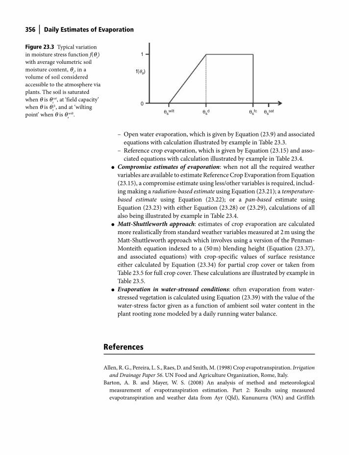
356 Daily Estimates of Evaporation
– Open water evaporation, which is given by Equation (23.9) and associated
equations with calculation illustrated by example in Table 23.3.
– Reference crop evaporation, which is given by Equation (23.15) and asso-
ciated equations with calculation illustrated by example in Table 23.4.
● Compromise estimates of evaporation: when not all the required weather
variables are available to estimate Reference Crop Evaporation from Equation
(23.15), a compromise estimate using less/other variables is required, includ-
ing making a radiation-based estimate using Equation (23.21); a temperature-
based estimate using Equation (23.22); or a pan-based estimate using
Equation (23.23) with either Equation (23.28) or (23.29), calculations of all
also being illustrated by example in Table 23.4.
● Matt-Shuttleworth approach: estimates of crop evaporation are calculated
more realistically from standard weather variables measured at 2 m using the
Matt-Shuttleworth approach which involves using a version of the Penman-
Monteith equation indexed to a (50 m) blending height (Equation (23.37),
and associated equations) with crop-specific values of surface resistance
either calculated by Equation (23.34) for partial crop cover or taken from
Table 23.5 for full crop cover. These calculations are illustrated by example in
Table 23.5.
● Evaporation in water-stressed conditions: often evaporation from water-
stressed vegetation is calculated using Equation (23.39) with the value of the
water-stress factor given as a function of ambient soil water content in the
plant rooting zone modeled by a daily running water balance.
References
Allen, R. G., Pereira, L. S., Raes, D. and Smith, M. (1998) Crop evapotranspiration. Irrigation
and Drainage Paper 56. UN Food and Agriculture Organization, Rome, Italy.
Barton, A. B. and Mayer, W. S. (2008) An analysis of method and meteorological
measurement of evapotranspiration estimation. Part 2: Results using measured
evapotranspiration and weather data from Ayr (Qld), Kununurra (WA) and Griffith
0
1
f(qs)
θswilt θsd θsfc θssat
Figure 23.3 Typical variation
in moisture stress function f(qs)
with average volumetric soil
moisture content, qs, in a
volume of soil considered
accessible to the atmosphere via
plants. The soil is saturated
when q is qssat, at ‘field capacity’
when q is qsfc, and at ‘wilting
point’ when q is qswilt.
Shuttleworth_c23.indd 356Shuttleworth_c23.indd 356 11/3/2011 6:41:03 PM11/3/2011 6:41:03 PM
Daily Estimates of Evaporation 357
(NSW). In: CRC for Irrigation Futures Technical Report No. 09−2/08, November 2008.
18pp.
Blaney, H. F. and Criddle, W. D. (1950) Determining water requirements in irrigated areas
from climatological and irrigation data. US Department of Agriculture Soil Conservation
Service TP−96, p. 48.
Blanken, P. D., Rouse, W. R., Culf, A. D., Spence, C., Boudreau, L. D., Jasper, J. N.,
Kochtubajda, R., Schertzer, W. M., Marsh, P. and Verseghy, D. (2000) Eddy covariance
measurements of evaporation from Great Slave Lake, Northwest Territories, Canada.
Water Resources Research, 36, 1069–1077.
Doorenbos, J. and Pruitt, W. O. (1977) Crop water requirements. Irrigation and Drainage
Paper, 24. Rome, Italy: United Nations Food and Agriculture Organization.
Finch, J. W. and Gash, J. H. C. (2002) Application of a simple finite difference model for
estimating evaporation from open water. Journal of Hydrology, 255, 253–259.
Hargreaves, G. H. (1975) Moisture availability and crop production. Transcripts of American
Society of Agricultural Engineers, 18 (5), 980–984.
Howell, T. A. and Evett, S. R. (2002) The Penman-Monteith Method. USDA-Agricultural
Research Service Conservation & Production Laboratory, Bushland, Texas, USA. http://
www.cprl.ars.usda.gov/wmru/pdfs/PM%20COLO%20Bar%202004%20corrected%20
9apr04.pdf
Inman-Bamber, N. G. and McGlinchey, M. G. (2003) Crop coefficients and water use esti-
mates for sugarcane based on long-term Bowen ratio energy balance measurements.
Field Crops Research, 83, 125–138.
Jensen, M. E., Burman, R. D. and Allen, R. G. (eds) (1990) Evapotranspiration and Irrigation
Water Requirements. ASCE Manuals and Reports on Engineering Practice No. 70, ASCE,
New York, p. 332.
Linacre, E. T. (1994) Estimating US Class A pan evaporation data from few climate data.
Water International, 19, 5–14.
Penman, H. L. (1948) Natural evaporation from open water, bare soil, and grass. Proceedings
of the Royal Society of London, Ser. A 193, 120−145.
Penman, H. L. (1963) Vegetation and hydrology, Technical Communication 53,
Commonwealth Bureau of Soils: Harpenden, England.
Roderick, M. L., Rotstayn, L. D., Farquhar, G. D. and Hobbins, M. T. (2007) On the attribu-
tion of changing pan evaporation. Geophysical Research Letters, 34, L17403.
doi:10.1029/2007GL031166.
Rotstayn, L. D., Roderick, M. L. and Farquhar, G. D. (2006) A simple pan-evaporation
model for analysis of climate simulations: Evaluation over Australia. Geophysical Research
Letters, 33, L17715. doi:17710.11029/12006GL027114.
Shuttleworth, W. J. (1993) Evaporation. In Maidment, D. (ed.) Handbook of Hydrology.
McGraw-Hill, New York.
Shuttleworth, W. J. (2006) Towards one-step estimation of crop water requirement.
Transactions of the ASABE, 49 (4), 925–935.
Shuttleworth, W. J. (2010) Back to the basics of understanding ET. In: Khan, S., Savenije, H.,
Demoth, S. and Hubert, P. (eds) Hydrocomplexity: New Tools for Solving Wicked Water
Problems: Kovacs Colloquium, July 2010. IAHS Publication No. 338, IAHS Press,
Wallingford, UK.
Shuttleworth, W. J. and Wallace, J. S. (2010) Calculating the water requirements of irrigated
crops in Australia using the Matt-Shuttleworth approach. Transactions of the ASABE, 52
(6),1895–1906.
Shuttleworth_c23.indd 357Shuttleworth_c23.indd 357 11/3/2011 6:41:03 PM11/3/2011 6:41:03 PM

358 Daily Estimates of Evaporation
Thom, A. S. and Oliver, H. R. (1977) On Penman’s equation for estimating evaporation.
Quarterly Journal of the Royal Meteorological Society, 103, 345–357.
Thom, A. S., Thony, J. L. and Vauclin, M. (1981) On the proper employment of evaporation
pans and atmometers in estimating potential transpiration. Quarterly Journal of the Royal
Meteorological Society, 107, 255–278.
Thornthwaite, C. W. (1948) An approach toward a rational classification of climate.
Geographical Review, 38, 55–94.
Wallace, J.S. (1995) Calculating evaporation: Resistance to factors. Agricultural and Forest
Meteorology, 73, 353–366.
Shuttleworth_c23.indd 358Shuttleworth_c23.indd 358 11/3/2011 6:41:03 PM11/3/2011 6:41:03 PM
Introduction
As previously mentioned, one important way that understanding of the interaction
between land surfaces and the ABL is used is in computer sub-models that become
important sub-components of meteorological, hydrological and/or coupled
atmospheric-hydro-ecological models. These sub-models are often called ‘soil
vegetation atmosphere schemes’ (SVATS) or, when used in meteorological models,
‘land-surface parameterization schemes’ (LSPs). They are important in atmospheric
models to specify the lower boundary condition, in hydrological models to specify
the upper boundary condition, and in coupled models as the essential interface
between model components.
Again, as previously mentioned, the availability of frequently sampled weather
variables from which SVATS can calculate surface exchanges is not usually an issue
because, in the case of meteorological models and coupled surface-atmosphere
models, the required variables are themselves regularly calculated by the remain-
der of the model and, in the case of hydrological models, the use of SVATS would
likely not be attempted unless the required data are available from measurements,
perhaps made with one or more automatic weather stations.
Basis and origin of land-surface sub-models
Putting aside for the moment the important indirect influence of terrestrial
vegetation on the concentration of atmospheric CO2, continental surfaces
influence the atmosphere in two main ways, (i) via the surface energy balance and
(ii) through the efficiency with which momentum is transferred to the ground
from the moving air. In the case of the surface energy balance, this influence is
exerted both through land surface characteristics that control the net capture of
24 Soil Vegetation Atmosphere Transfer Schemes
Terrestrial Hydrometeorology, First Edition. W. James Shuttleworth.
© 2012 John Wiley & Sons, Ltd. Published 2012 by John Wiley & Sons, Ltd.
Shuttleworth_c24.indd 359Shuttleworth_c24.indd 359 11/3/2011 6:39:34 PM11/3/2011 6:39:34 PM
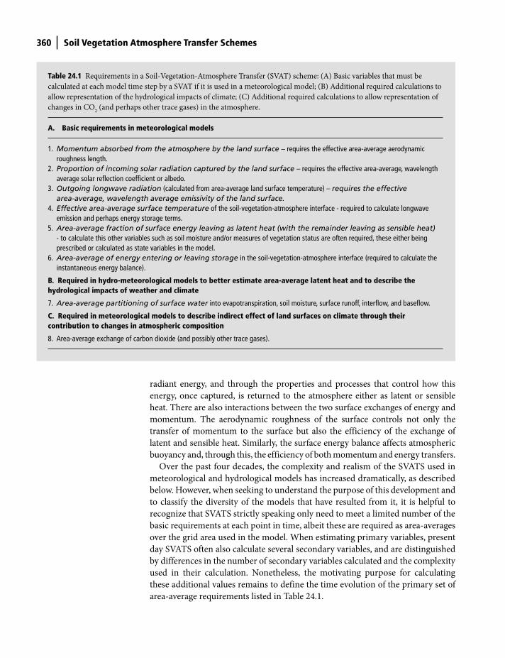
360 Soil Vegetation Atmosphere Transfer Schemes
radiant energy, and through the properties and processes that control how this
energy, once captured, is returned to the atmosphere either as latent or sensible
heat. There are also interactions between the two surface exchanges of energy and
momentum. The aerodynamic roughness of the surface controls not only the
transfer of momentum to the surface but also the efficiency of the exchange of
latent and sensible heat. Similarly, the surface energy balance affects atmospheric
buoyancy and, through this, the efficiency of both momentum and energy transfers.
Over the past four decades, the complexity and realism of the SVATS used in
meteorological and hydrological models has increased dramatically, as described
below. However, when seeking to understand the purpose of this development and
to classify the diversity of the models that have resulted from it, it is helpful to
recognize that SVATS strictly speaking only need to meet a limited number of the
basic requirements at each point in time, albeit these are required as area-averages
over the grid area used in the model. When estimating primary variables, present
day SVATS often also calculate several secondary variables, and are distinguished
by differences in the number of secondary variables calculated and the complexity
used in their calculation. Nonetheless, the motivating purpose for calculating
these additional values remains to define the time evolution of the primary set of
area-average requirements listed in Table 24.1.
Table 24.1 Requirements in a Soil-Vegetation-Atmosphere Transfer (SVAT) scheme: (A) Basic variables that must be
calculated at each model time step by a SVAT if it is used in a meteorological model; (B) Additional required calculations to
allow representation of the hydrological impacts of climate; (C) Additional required calculations to allow representation of
changes in CO2 (and perhaps other trace gases) in the atmosphere.
A. Basic requirements in meteorological models
1. Momentum absorbed from the atmosphere by the land surface – requires the effective area-average aerodynamic roughness length.
2. Proportion of incoming solar radiation captured by the land surface – requires the effective area-average, wavelength average solar reflection coefficient or albedo.
3. Outgoing longwave radiation (calculated from area-average land surface temperature) – requires the effective area-average, wavelength average emissivity of the land surface.
4. Effective area-average surface temperature of the soil-vegetation-atmosphere interface - required to calculate longwave emission and perhaps energy storage terms.
5. Area-average fraction of surface energy leaving as latent heat (with the remainder leaving as sensible heat) - to calculate this other variables such as soil moisture and/or measures of vegetation status are often required, these either being prescribed or calculated as state variables in the model.
6. Area-average of energy entering or leaving storage in the soil-vegetation-atmosphere interface (required to calculate the instantaneous energy balance).
B. Required in hydro-meteorological models to better estimate area-average latent heat and to describe the hydrological impacts of weather and climate
7. Area-average partitioning of surface water into evapotranspiration, soil moisture, surface runoff, interflow, and baseflow.
C. Required in meteorological models to describe indirect effect of land surfaces on climate through their contribution to changes in atmospheric composition
8. Area-average exchange of carbon dioxide (and possibly other trace gases).
Shuttleworth_c24.indd 360Shuttleworth_c24.indd 360 11/3/2011 6:39:35 PM11/3/2011 6:39:35 PM

Soil Vegetation Atmosphere Transfer Schemes 361
Originally, land surface models (e.g., Manabe et al., 1965; Shukla and Mintz,
1982) were as simple as they could be. They ignored energy storage in the soil-
vegetation-atmosphere interface (Table 24.1, value 6), and did not calculate a
detailed surface water partition (Table 24.1, value 7) or carbon dioxide exchange
(Table 24.1, value 8). They simply assumed typical fixed values of aerodynamic
roughness length, albedo, and surface emissivity and applied these to all continental
surfaces to calculate values 1, 2, 3, 4 and 5 in Table 24.1.
In early models, energy sharing between latent and sensible heat and (implicitly)
the surface temperature (requirements 4 and 5) was calculated using a simple
‘Budyko Bucket’ model (Budyko, 1948; 1956), see Fig. 24.1. A form of potential
evaporation rate was assumed and calculated using the Penman-Monteith
equation assuming zero surface resistance and an aerodynamic resistance equal to
that for momentum transfer in neutral conditions with the assigned aerodynamic
roughness length. The actual evaporation rate was then calculated at any point in
time by making a running water balance of the water level in a hypothetical
‘bucket’ located at the land surface, which is filled by precipitation and emptied by
evaporation and, when the water depth, d, stored in the bucket exceeds a critical
value, dmax
, also by runoff. The actual evaporation rate was assumed to vary linearly
with the fractional fill of this bucket between zero and the calculated potential
evaporation rate.
Early evidence for land-surface influences on climate came through model
experiments made with General Circulation Models (GCMs) which used the
simple model just described. These experiments involved making imposed
changes in the values of one of the (few) parameters used in these simple SVATS
and comparing the model-simulated climates before and after such a change.
The first such study was made by Charney et al. (1975) and was motivated by
the hypothesis (Fig. 24.2a) that expansion of desert regions, especially those in
the Sahel region of Africa, might result from a human-induced, land-surface
Precipitation, P
FieldCapacity
WaterDepth
dmax
d
Evaporation, E = bEp
Runoff, R
1
b
0
∂d
If d′ > dmax d → dmax and R = (d ′ − dmax)
= P − E∂t
d0 dmax
Figure 24.1 Schematic diagram of the SVATS used in early studies of the effect of land surfaces on weather and climate
based on the ‘Budyko Bucket’.
Shuttleworth_c24.indd 361Shuttleworth_c24.indd 361 11/3/2011 6:39:35 PM11/3/2011 6:39:35 PM
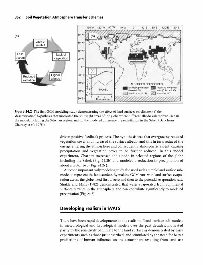
362 Soil Vegetation Atmosphere Transfer Schemes
driven positive feedback process. The hypothesis was that overgrazing reduced
vegetation cover and increased the surface albedo, and this in turn reduced the
energy entering the atmosphere and consequently atmospheric ascent, causing
precipitation and vegetation cover to be further reduced. In this model
experiment, Charney increased the albedo in selected regions of the globe
including the Sahel, (Fig. 24.2b) and modeled a reduction in precipitation of
about a factor two (Fig. 24.2c).
A second important early modeling study also used such a simple land surface sub-
model to represent the land surface. By making GCM runs with land surface evapo-
ration across the globe fixed first to zero and then to the potential evaporation rate,
Shukla and Minz (1982) demonstrated that water evaporated from continental
surfaces recycles in the atmosphere and can contribute significantly to modeled
precipitation (Fig. 24.3).
Developing realism in SVATS
There have been rapid developments in the realism of land-surface sub-models
in meteorological and hydrological models over the past decades, motivated
partly by the sensitivity of climate to the land surface as demonstrated by early
experiments such as those just described, and stimulated by the need for better
predictions of human influence on the atmosphere resulting from land use
160°W
80°N
60°N
40°N
20°N
0°
20°S
40°S
60°S
(c)
(b)
Reducedradiation
Lessascent
Higheralbedo
Lack ofvegetation
Lack ofrainfall
(a)
80°S Time (weeks)
Humid area (0.14) Ice cover (0.7)
Idealised permanentdesert (0.35)
ALBEDOES PRESCRIBEDIdealised margionalarea (0.14 or 0.35)
Pre
cipi
tatio
n (m
m d
−1)
SAHEL
10
2
4
6
2 3 4
120°W 80°W 40°W 0° 40°E 80°E 120°E 160°E
Figure 24.2 The first GCM modeling study demonstrating the effect of land surfaces on climate: (a) the
‘desertification’ hypothesis that motivated the study; (b) areas of the globe where different albedo values were used in
the model, including the Sahelian region; and (c) the modeled difference in precipitation in the Sahel. (Data from
Charney et al., 1975.)
Shuttleworth_c24.indd 362Shuttleworth_c24.indd 362 11/3/2011 6:39:35 PM11/3/2011 6:39:35 PM
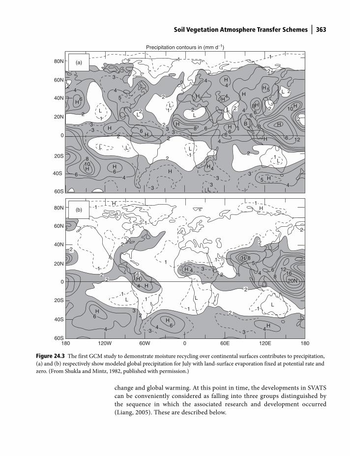
Soil Vegetation Atmosphere Transfer Schemes 363
change and global warming. At this point in time, the developments in SVATS
can be conveniently considered as falling into three groups distinguished by
the sequence in which the associated research and development occurred
(Liang, 2005). These are described below.
44
4
36
1
8
31
1
(b)
45
3
1
6
106
B
54
44
8 6
445
3
6
33
810
64
3
4
46 6
6
B
H
3
6
(a)
18060S
40S
20S
0
20N
40N
60N
80N
60S
40S
20S
0
20N
40N
60N
80N
120W 60W 0 60E 120E 180
L
H
2
2
2
2
2
22
2
2
1 H
H
H
L
H 3
H2
H
HH
H
HH
L1
HH
H
B
H
HH
H
H
LL
L
L
1
L
H
H
2
2
6H
H
H
L
H
L
1
1
H
LL1
1
1
3
2
L
L
4
4
43
568
1216
20N
116
6
1
11
1
2L
12
2
2
422
2
23
2
2
2
2
2
3
Precipitation contours in (mm d−1)
Figure 24.3 The first GCM study to demonstrate moisture recycling over continental surfaces contributes to precipitation,
(a) and (b) respectively show modeled global precipitation for July with land-surface evaporation fixed at potential rate and
zero. (From Shukla and Mintz, 1982, published with permission.)
Shuttleworth_c24.indd 363Shuttleworth_c24.indd 363 11/3/2011 6:39:37 PM11/3/2011 6:39:37 PM

364 Soil Vegetation Atmosphere Transfer Schemes
Plot-scale, one-dimensional ‘micrometeorological’ models
Following the use of the Budyko Bucket model, the next generation of SVATS can be
characterized by the developments of Deardorff (1978), who made simplifying
improvements in the representation of soil heat fluxes through the ‘force-restore’
scheme, and Dickinson et al. (1986) and Sellers et al. (1986), who made substantial
improvements in the representation of vegetation controls on evaporation. The
essential essence of this group of SVATS which is illustrated schematically in
Fig. 24.4, is that they were one-dimensional representations of the micrometeoro-
logical interaction of uniform plots of vegetation, but applied at the (much larger)
grid scale used in GCMs.
Notably among the improvements in vegetation-related features was the
introduction of the effect of leaf stomatal resistance through development of the
Monteith (1965) ‘big leaf ’ assumption and of a canopy water balance to calculate
interception loss using a (usually simplified) version of the Rutter model, both of
which were described in Chapter 22. In this group of SVATS, the temperature of
the vegetation was also sometimes calculated explicitly as a state variable, and dry
canopy surface resistance was usually either assumed constant for a particular
vegetation cover, or parameterized in terms of a series of stress factors in a version
of the Jarvis-Stewart model (see, for example, Shuttleworth, 1989) in which surface
resistance is expressed in the form:
0
1 s c R D T M
s
g g g g g g gr
= =
(24.1)
lE
lE
lEH
H
H Sr
Lu
Lu
LuSr
Sr lEH
Lu
SrlE
H
Lu
Sr
P S Ld
Runoff
Runoff
RunoffRunoff
Bare soil
Snow pack
Deep drainageDeep drainage
Deep drainage
Deep drainage
Figure 24.4 Schematic
diagram of second
generation one-dimensional
SVATs in which a plot-scale
micrometeorological model
with an explicit vegetation
canopy was applied at grid
scale. See Plate 3 for a colour
version of this image.
Shuttleworth_c24.indd 364Shuttleworth_c24.indd 364 11/3/2011 6:39:37 PM11/3/2011 6:39:37 PM
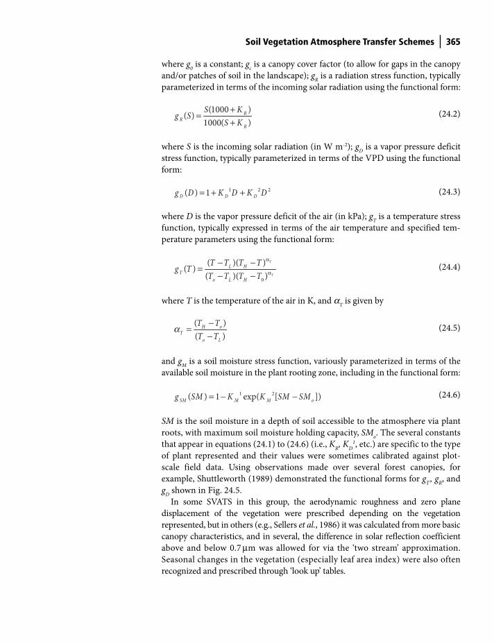
Soil Vegetation Atmosphere Transfer Schemes 365
where g0 is a constant; g
c is a canopy cover factor (to allow for gaps in the canopy
and/or patches of soil in the landscape); gR is a radiation stress function, typically
parameterized in terms of the incoming solar radiation using the functional form:
(1000 )( )
1000( )R
RR
S Kg SS K
+=
+
(24.2)
where S is the incoming solar radiation (in W m-2); gD is a vapor pressure deficit
stress function, typically parameterized in terms of the VPD using the functional
form:
1 2 2( ) 1D D Dg D K D K D= + +
(24.3)
where D is the vapor pressure deficit of the air (in kPa); gT is a temperature stress
function, typically expressed in terms of the air temperature and specified tem-
perature parameters using the functional form:
0
( )( )( )
( )( )
T
T
L HT
o L H
T T T Tg TT T T T
α
α
− −=
− −
(24.4)
where T is the temperature of the air in K, and aT is given by
( )
( )H o
To L
T TT T
−=
−a
(24.5)
and gM
is a soil moisture stress function, variously parameterized in terms of the
available soil moisture in the plant rooting zone, including in the functional form:
1 2( ) 1 exp( [ ])SM M M og SM K K SM SM= − −
(24.6)
SM is the soil moisture in a depth of soil accessible to the atmosphere via plant
roots, with maximum soil moisture holding capacity, SMo. The several constants
that appear in equations (24.1) to (24.6) (i.e., KR, K
D1, etc.) are specific to the type
of plant represented and their values were sometimes calibrated against plot-
scale field data. Using observations made over several forest canopies, for
example, Shuttleworth (1989) demonstrated the functional forms for gT , g
R, and
gD shown in Fig. 24.5.
In some SVATS in this group, the aerodynamic roughness and zero plane
displacement of the vegetation were prescribed depending on the vegetation
represented, but in others (e.g., Sellers et al., 1986) it was calculated from more basic
canopy characteristics, and in several, the difference in solar reflection coefficient
above and below 0.7 μm was allowed for via the ‘two stream’ approximation.
Seasonal changes in the vegetation (especially leaf area index) were also often
recognized and prescribed through ‘look up’ tables.
Shuttleworth_c24.indd 365Shuttleworth_c24.indd 365 11/3/2011 6:39:39 PM11/3/2011 6:39:39 PM
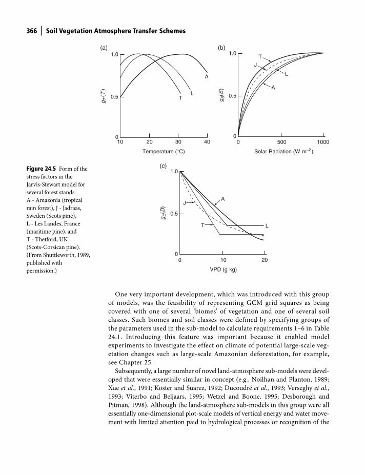
366 Soil Vegetation Atmosphere Transfer Schemes
One very important development, which was introduced with this group
of models, was the feasibility of representing GCM grid squares as being
covered with one of several ‘biomes’ of vegetation and one of several soil
classes. Such biomes and soil classes were defined by specifying groups of
the parameters used in the sub-model to calculate requirements 1–6 in Table
24.1. Introducing this feature was important because it enabled model
experiments to investigate the effect on climate of potential large-scale veg-
etation changes such as large-scale Amazonian deforestation, for example,
see Chapter 25.
Subsequently, a large number of novel land-atmosphere sub-models were devel-
oped that were essentially similar in concept (e.g., Noilhan and Planton, 1989;
Xue et al., 1991; Koster and Suarez, 1992; Ducoudré et al., 1993; Verseghy et al.,
1993; Viterbo and Beljaars, 1995; Wetzel and Boone, 1995; Desborough and
Pitman, 1998). Although the land-atmosphere sub-models in this group were all
essentially one-dimensional plot-scale models of vertical energy and water move-
ment with limited attention paid to hydrological processes or recognition of the
(a)
403020
Temperature (°C)
100
0.5 TL
A
g T(T
)
1.0(b)
Solar Radiation (W m−2)
g S(S
)
00 500 1000
0.5
1.0
A
L
T
J
(c)g D
(D)
00 10
VPD (g kg)
20
0.5
J
1.0
T
A
L
Figure 24.5 Form of the
stress factors in the
Jarvis-Stewart model for
several forest stands:
A - Amazonia (tropical
rain forest), J - Jadraas,
Sweden (Scots pine),
L - Les Landes, France
(maritime pine), and
T - Thetford, UK
(Scots-Corsican pine).
(From Shuttleworth, 1989,
published with
permission.)
Shuttleworth_c24.indd 366Shuttleworth_c24.indd 366 11/3/2011 6:39:43 PM11/3/2011 6:39:43 PM
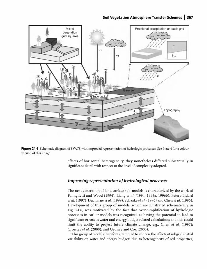
Soil Vegetation Atmosphere Transfer Schemes 367
effects of horizontal heterogeneity, they nonetheless differed substantially in
significant detail with respect to the level of complexity adopted.
Improving representation of hydrological processes
The next generation of land surface sub-models is characterized by the work of
Famiglietti and Wood (1994), Liang et al. (1994; 1996a, 1996b), Peters-Lidard
et al. (1997), Ducharne et al. (1999), Schaake et al. (1996) and Chen et al. (1996).
Development of this group of models, which are illustrated schematically in
Fig. 24.6, was motivated by the fact that over-simplification of hydrologic
processes in earlier models was recognized as having the potential to lead to
significant errors in water and energy budget related calculations and this could
limit the ability to project future climate change, e.g., Chen et al. (1997);
Crossley et al. (2000); and Gedney and Cox (2003).
This group of models therefore attempted to address the effects of subgrid spatial
variability on water and energy budgets due to heterogeneity of soil properties,
Mixedvegetation
grid squares
S
lE
lElE
lE
H
HH
H
Sr
SrSr
Sr
Snow pack
Water table
Bare soil
P
m
1-m
Fractional precipitation on each grid
Topography
Lu
Lu
Lu
Lu
Ld
Figure 24.6 Schematic diagram of SVATS with improved representation of hydrologic processes. See Plate 4 for a colour
version of this image.
Shuttleworth_c24.indd 367Shuttleworth_c24.indd 367 11/3/2011 6:39:44 PM11/3/2011 6:39:44 PM
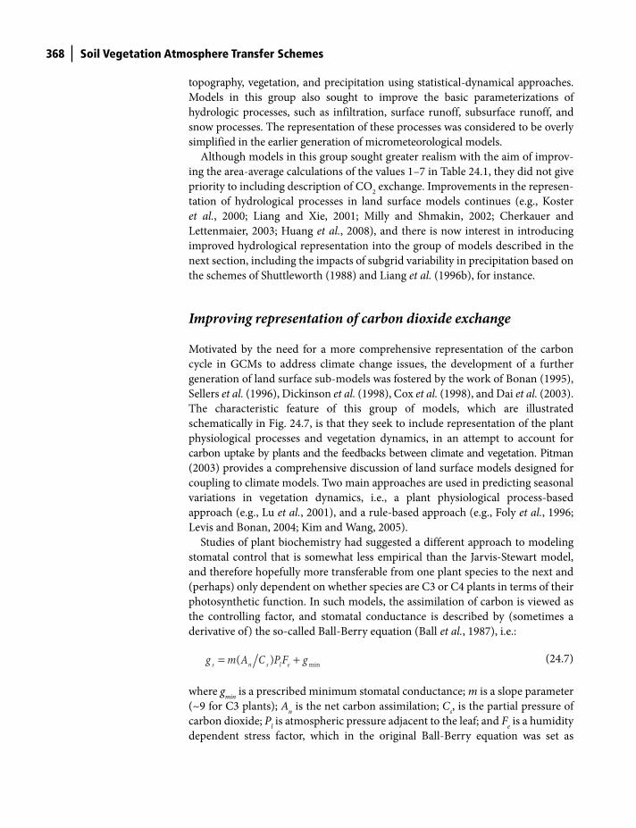
368 Soil Vegetation Atmosphere Transfer Schemes
topography, vegetation, and precipitation using statistical-dynamical approaches.
Models in this group also sought to improve the basic parameterizations of
hydrologic processes, such as infiltration, surface runoff, subsurface runoff, and
snow processes. The representation of these processes was considered to be overly
simplified in the earlier generation of micrometeorological models.
Although models in this group sought greater realism with the aim of improv-
ing the area-average calculations of the values 1–7 in Table 24.1, they did not give
priority to including description of CO2 exchange. Improvements in the represen-
tation of hydrological processes in land surface models continues (e.g., Koster
et al., 2000; Liang and Xie, 2001; Milly and Shmakin, 2002; Cherkauer and
Lettenmaier, 2003; Huang et al., 2008), and there is now interest in introducing
improved hydrological representation into the group of models described in the
next section, including the impacts of subgrid variability in precipitation based on
the schemes of Shuttleworth (1988) and Liang et al. (1996b), for instance.
Improving representation of carbon dioxide exchange
Motivated by the need for a more comprehensive representation of the carbon
cycle in GCMs to address climate change issues, the development of a further
generation of land surface sub-models was fostered by the work of Bonan (1995),
Sellers et al. (1996), Dickinson et al. (1998), Cox et al. (1998), and Dai et al. (2003).
The characteristic feature of this group of models, which are illustrated
schematically in Fig. 24.7, is that they seek to include representation of the plant
physiological processes and vegetation dynamics, in an attempt to account for
carbon uptake by plants and the feedbacks between climate and vegetation. Pitman
(2003) provides a comprehensive discussion of land surface models designed for
coupling to climate models. Two main approaches are used in predicting seasonal
variations in vegetation dynamics, i.e., a plant physiological process-based
approach (e.g., Lu et al., 2001), and a rule-based approach (e.g., Foly et al., 1996;
Levis and Bonan, 2004; Kim and Wang, 2005).
Studies of plant biochemistry had suggested a different approach to modeling
stomatal control that is somewhat less empirical than the Jarvis-Stewart model,
and therefore hopefully more transferable from one plant species to the next and
(perhaps) only dependent on whether species are C3 or C4 plants in terms of their
photosynthetic function. In such models, the assimilation of carbon is viewed as
the controlling factor, and stomatal conductance is described by (sometimes a
derivative of) the so-called Ball-Berry equation (Ball et al., 1987), i.e.:
min( )s n s l eg m A C P F g= +
(24.7)
where gmin
is a prescribed minimum stomatal conductance; m is a slope parameter
(~9 for C3 plants); An is the net carbon assimilation; C
s, is the partial pressure of
carbon dioxide; Pl is atmospheric pressure adjacent to the leaf; and F
e is a humidity
dependent stress factor, which in the original Ball-Berry equation was set as
Shuttleworth_c24.indd 368Shuttleworth_c24.indd 368 11/3/2011 6:39:44 PM11/3/2011 6:39:44 PM
Soil Vegetation Atmosphere Transfer Schemes 369
numerically equal to the relative humidity, but which in some SVATS (e.g.,
Dickinson et al., 1998), is assumed to be a function of vapor-pressure deficit. The
introduction of this alternative means of describing the behavior of stomata has
sometimes been referred to as the ‘greening of SVATS’. In this formula, the simplest
estimate of An, is given (Farquhar and Sharkey, 1982) by:
min( , , )n c e sA J J J=
(24.8)
where Jc , J
e , J
s are functions expressing the assimilation rates when limited by the
Rubisco enzyme, light, and transport capacity, respectively, for C3 and C4 plants;
see Collatz et al. (1991; 1992), Sellers et al. (1996) and Cox et al. (2001). In practice,
it has been observed that the transition between these three limiting rates is not
abrupt but gradual, and some SVATS (e.g., Collatz et al., 1991; Cox et al., 2001)
have devised mathematical ways to simulate this smooth transition.
Thus, a key difference between the Ball-Berry formula for stomatal conductance
(resistance) and the Jarvis-Stewart formula is that stress factors (apart from that
for humidity) are no longer combined as a product; rather, one factor is considered
to be the dominant limitation on carbon assimilation and hence on stomatal
conductance. SVATS continue to make progress in describing vegetation and are
Vegetationdynamics Vegetation
growth cycle
CO2
N2
lE
lE
lE
H
H
H Sr
Lu
Lu
Sr
Sr lEH
Lu
SrlE
H
Lu
Sr
PS Ld
Runoff
Snow packRunoff
RunoffRunoff
Bare soil
Deep drainageDeep drainage
Deep drainage
Deep drainage
Figure 24.7 Schematic diagram of SVATS with improved representation of vegetation related processes, including CO2
exchange and ecosystem evolution. See Plate 5 for a colour version of this image.
Shuttleworth_c24.indd 369Shuttleworth_c24.indd 369 11/3/2011 6:39:45 PM11/3/2011 6:39:45 PM
370 Soil Vegetation Atmosphere Transfer Schemes
now seeking to describe the evolution of the biome (i.e., vegetation cover)
represented in the GCM at a particular place in response to long-term changes in
modeled climate (Foley et al., 1996; 2000; Cox et al., 2000; 2001; Kucharik et al.,
2000; Oyama and Nobre, 2003; 2004). Ultimately this capability may also become
relevant in long-term, large-scale hydrological modeling studies.
As yet, this group of sub-models does not consider interactions between the
biogeochemical cycles of carbon, nitrogen and phosphorus. In fact, such
interactions are not yet considered in many terrestrial biogeochemical
models, including the CENTURY model (Wang et al., 2007). However, including
such interactions is likely necessary for a more comprehensive and realistic
representation of the effect of land surface processes on the carbon cycle. It is also
true that most of the land surface models in this group of sub-models have simpler
treatments of sub-grid spatial variability and hydrological processes than those
described in the last section. Consequently, there is a need to combine the model
improvements in describing hydrological processes with those describing carbon
dioxide exchange and vegetation dynamics in a new generation of land surface
sub-models. Fortunately, ecologists, climatologists, and hydrologists have begun
to work together to improve the realism and functionality of SVATS.
Ongoing developments in land surface sub-models
The impacts of surface and groundwater interactions on the land-atmosphere sys-
tem have hitherto received little attention, but recognizing the role roots (especially
deep roots) may play in the plant-soil-land continuum, researchers have now begun
to investigate the dynamic interactions of surface water and groundwater, and
whether such interactions can affect vegetation and, via vegetation, land-atmos-
phere interactions (e.g., Winter, 2001; Gutowski et al., 2002; York et al., 2002; Liang
et al., 2003; 2006; Maxwell and Miller, 2005; Yeh and Eltahir, 2005; Fan et al., 2007;
Niu et al., 2007). Several different approaches are under investigation, including:
(a) A ‘TOP model’ type based approach (e.g., Walko et al., 2000).
(b) Solving for soil moisture in unsaturated zones and pressure head profiles in
saturated zones separately by applying (variations of) the Richards equa-
tion to each zone respectively (e.g., Gutowski et al., 2002; York et al., 2002;
Yeh and Eltahir, 2005; Fan et al., 2007; Niu et al., 2007). In this approach,
the coupling is essentially one-way rather than two-way.
(c) Solving for the hydraulic pressure profile for the unsaturated and saturated
zones together based on a mixed form of the Richards equation (e.g.,
Maxwell and Miller, 2005). This approach involves two-way coupling.
(d) Solving for soil moisture profile by applying the Richards equation to the
unsaturated zone only, with the groundwater table treated as a moving
boundary (e.g., Liang et al., 2003). This relatively simple approach does not
introduce any additional parameters other than those already used by a
typical land surface model and also involves two-way coupling.
Shuttleworth_c24.indd 370Shuttleworth_c24.indd 370 11/3/2011 6:39:47 PM11/3/2011 6:39:47 PM
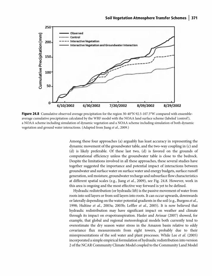
Soil Vegetation Atmosphere Transfer Schemes 371
Among these four approaches (a) arguably has least accuracy in representing the
dynamic movement of the groundwater table, and the two-way coupling in (c) and
(d) is likely preferable. Of these last two, (d) is favored on the grounds of
computational efficiency unless the groundwater table is close to the bedrock.
Despite the limitations involved in all these approaches, these several studies have
together suggested the importance and potential impact of interactions between
groundwater and surface water on surface water and energy budgets, surface runoff
generation, soil moisture, groundwater recharge and subsurface flow characteristics
at different spatial scales (e.g., Jiang et al., 2009), see Fig. 24.8. However, work in
this area is ongoing and the most effective way forward is yet to be defined.
Hydraulic redistribution (or hydraulic lift) is the passive movement of water from
roots into soil layers or from soil layers into roots. It can occur upwards, downwards
or laterally depending on the water potential gradients in the soil (e.g., Burgess et al.,
1998; Hultine et al., 2003a; 2003b; Leffler et al., 2005). It is now believed that
hydraulic redistribution may have significant impact on weather and climate
through its impact on evapotranspiration. Hasler and Avissar (2007) showed, for
example, that global and regional meteorological models both currently tend to
overestimate the dry season water stress in the Amazon basin relative to eddy
covariance flux measurements from eight towers, probably due to their
misrepresentations of the soil water and plant processes. While Lee et al. (2005)
incorporated a simple empirical formulation of hydraulic redistribution into version
2 of the NCAR Community Climate Model coupled to the Community Land Model
Figure 24.8 Cumulative observed average precipitation for the region 30-40°N 92.5-107.5°W compared with ensemble-
average cumulative precipitation calculated by the WRF model with the NOAA land surface scheme (labeled ‘control’),
a NOAA scheme including simulation of dynamic vegetation and a NOAA scheme including simulation of both dynamic
vegetation and ground water interactions. (Adapted from Jiang et al., 2009.)
Shuttleworth_c24.indd 371Shuttleworth_c24.indd 371 11/3/2011 6:39:47 PM11/3/2011 6:39:47 PM
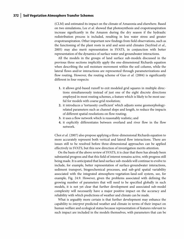
372 Soil Vegetation Atmosphere Transfer Schemes
(CLM) and estimated its impact on the climate of Amazonia and elsewhere. Based
on two simulations, Lee et al. showed that photosynthesis and evapotranspiration
increase significantly in the Amazon during the dry season if the hydraulic
redistribution process is included, resulting in less water stress and greater
evapotranspiration. Other important new findings from field observations, such as
the functioning of the plant roots in arid and semi-arid climates (Seyfried et al.,
2005) may also merit representation in SVATS, in conjunction with better
representation of the dynamics of surface water and groundwater interactions.
All the models in the groups of land surface sub-models discussed in the
previous three sections implicitly apply the one-dimensional Richards equation
when describing the soil moisture movement within the soil column, while the
lateral flows and/or interactions are represented through parameterizations and
flow routing. However, the routing scheme of Guo et al. (2004) is significantly
different in four respects:
1. it allows grid-based runoff to exit modeled grid squares in multiple direc-
tions simultaneously instead of just one of the eight discrete directions
employed in most routing schemes, a feature which is likely to be most use-
ful for models with coarse grid resolution;
2. it introduces a ‘tortuosity coefficient’ which adjusts some geomorphology-
related parameters such as channel slope and length, to reduce the impacts
of different spatial resolutions on flow routing;
3. it uses a flow network which is reasonably realistic; and
4. it explicitly differentiates between overland and river flow in the flow
network.
Choi et al. (2007) also propose applying a three-dimensional Richards equation to
more accurately represent both vertical and lateral flow interactions. There are
issues still to be resolved before three-dimensional approaches can be applied
effectively in SVATS, but this new direction of investigation merits attention.
On the basis of the above review of SVATS, it is clear that there has already been
substantial progress and that this field of interest remains active, with progress still
being made. It is anticipated that land surface sub-models will continue to evolve to
include, for example, better representation of surface-groundwater interactions,
sediment transport, biogeochemical processes, and sub-grid spatial variability
associated with the integrated atmosphere-vegetation-land-soil system, see, for
example, Fig. 24.9. However, given the problems associated with defining the
growing number of parameters that will need to be specified globally in such
models, it is not yet clear that further development and associated sub-model
complexity will necessarily have a major positive impact on the accuracy and
reliability with which predictions of weather and climate can be made.
What is arguably more certain is that further development may enhance the
capability to interpret predicted weather and climate in terms of their impact on
human welfare and ecological status because representation of features relevant to
such impact are included in the models themselves, with parameters that can be
Shuttleworth_c24.indd 372Shuttleworth_c24.indd 372 11/3/2011 6:39:47 PM11/3/2011 6:39:47 PM
Soil Vegetation Atmosphere Transfer Schemes 373
locally calibrated. Further development may thus be a mechanism through which
meteorologists, hydrologists, biologists and ecologists can be brought together
with applications specialists concerned with the management of water, agricul-
tural and industrial resources and public health.
Important points in this chapter
● Purpose of SVATS: is to specify the lower boundary conditions in atmospheric
models, the upper boundary conditions in hydrological models, or provide
the interface between land surfaces and the atmosphere in coupled models.
● Function of SVATS: is to calculate the exchange of energy, water, and carbon
dioxide and perhaps also other trace gases between land surfaces and the
atmosphere, and sometimes also components of the surface water balance
from ‘forcing data’ that comprises frequently sampled (either modeled or
measured) values of near-surface weather variables.
Mixed vegetationwith vegetation
dynamics
SLd
(CO2, N2,...)
Snowpack
Routing
Dataassimilation
m
1-m
Fractional precipitation on each grid
Routing
(CO2, N2,...)
LuLu
SrSr
HH
lElE
Figure 24.9 Schematic diagram of potential future developments in SVATS. See Plate 6 for a colour version of this image.
Shuttleworth_c24.indd 373Shuttleworth_c24.indd 373 11/3/2011 6:39:48 PM11/3/2011 6:39:48 PM
374 Soil Vegetation Atmosphere Transfer Schemes
● Requirements from SVATS: modern SVATS can be complex and may calculate
many variables but the motivating purpose for calculating these additional
values remains to calculate the time evolution of the limited set of area-
average requirements listed in Table 24.1.
● Early SVATS: originally SVATS prescribed fixed, globally-applied surface
parameters (e.g., surface roughness, albedo, emissivity, etc.) and used a sim-
ple ‘bucket model’ for surface energy partition, but using these in GCMs
demonstrated the sensitivity of modeled climate to changes in these
parameters.
● Micrometeorological SVATS: subsequent development resulted in a genera-
tion of SVATS, here called ‘micrometeorological’ SVATS, that were fairly
detailed one-dimensional models of the interactions of different uniform
vegetation canopies that strictly only apply at the scale of a few hundred
meters.
● Hydrological improvements in SVATS: further development sought
improvements in SVATS’ ability to describe hydrological processes,
including:
— improving basic parameterizations of hydrologic processes such as
infiltration, surface runoff, subsurface runoff and snow processes;
— representing the effects of subgrid spatial variability due to heteroge-
neity of soil properties, topography, vegetation and precipitation using
statistical-dynamical approaches.
● ‘Greening’ of SVATS: recognition of potential climate change caused a major
shift in direction in SVAT development toward providing improved capabil-
ity to simulate CO2 exchange, and this shift resulted in a substantial revision
in the preferred representation of plant stomatal behavior in SVATS (e.g.,
from the Jarvis-Stewart to the Ball-Berry parameterization).
● Ongoing development of SVATS: current development is concerned with
addressing more difficult aspects of surface-atmosphere interactions includ-
ing the impacts of surface-groundwater interactions on the land-atmosphere
system, and hydraulic redistribution (or hydraulic lift).
● Future value of SVAT development: further developments of SVATS that
add complexity will not necessarily improve their performance in climate
and weather prediction, more likely it will improve ability to interpret pre-
dicted weather and climate in terms of their impact on human welfare and
ecological status.
References
Ball J.T., Woodrow I.E. and Berry J.A. (1987) A model predicting stomatal conductance and
its contribution to the control of photosynthesis under different environmental
conditions. In: Biggins, I. (ed.), Progress in Photosynthesis Research, vol. IV pp. 221–224.
Martinus-Nijhoff Publishers, Dordrecht, The Netherlands.
Shuttleworth_c24.indd 374Shuttleworth_c24.indd 374 11/3/2011 6:39:48 PM11/3/2011 6:39:48 PM
Soil Vegetation Atmosphere Transfer Schemes 375
Bonan, G.B. (1995) Land-atmosphere CO2 exchange simulated by a land surface process
model coupled to an atmospheric general circulation model. Journal of Geophysical
Research, 100 (D2), 2817–2831.
Budyko, M.I. (1948) Evaporation under Natural Conditions (in Russian). Gidrometeoizdat,
136 pp.
Budyko, M.I. (1956) The Heat Balance of the Earth’s Surface (in Russian). Gidrometeoizdat,
255 pp.
Burgess, S.S.O., Adams, M.A., Turner, N.C. and Ong, C.K. (1998) The redistribution of soil
water by tree root systems. Oecologia, 115, 306–311.
Charney, J., Stone, P.H. and Quirk, W.J. (1975) Drought in Sahara: a biophysical feedback
mechanism. Science, 187, 434–435.
Chen, F., Mitchell, K., Schaake, J., Xue, Y.K., Pan, H.L., Koren, V., Duan, Q.Y., Ek, M. and
Betts, A. (1996) Modeling of land surface evaporation by four schemes and comparison
with FIFE observations. Journal of Geophysical Research, 101 (D3), 7251–7268.
Chen, T.H., Henderson-Sellers, A., Milly, P.C.D., Pitman, A.J., Beljaars, A.C.M., Polcher, J.,
Abramopoulos, F., Boone, A., Chang, S., Chen, F., Dai, Y., Desborough, C.E., Dickinson, R.E.,
Dümenil, L., Ek, M., Garratt, J.R., Gedney, N., Gusev, Y.M., Kim, J., Koster, R.,
Kowalczyk, E.A., Laval, K., Lean, J., Lettenmaier, D., Liang, X., Mahfouf, J.-F.,
Mengelkamp, H.-T., Mitchell, K., Nasonova, O.N., Noilhan, J., Robock, A., Rosenzweig, C.,
Schaake, J., Schlosser, C.A., Schulz, J.-P., Shao, Y., Shmakin, A.B., Verseghy, D.L., Wetzel, P.,
Wood, E.F., Xue, Y., Yang, Z.-L. and Zeng, Q. (1997) Cabauw experimental results from
the project for intercomparison of land-surface parameterization schemes, Journal of
Climate, 10(6), 1194–1215.
Cherkauer, K.A. and Lettenmaier, D.P. (2003) Simulation of spatial variability in snow and
frozen soil. Journal of Geophysical Research, 108 (D22), 8858, doi:10.1029/2003JD003575.
Choi, H.I., Kumar, P. and Liang, X.Z. (2007) Three-dimensional volume-averaged soil
moisture transport model with a scalable parameterization of subgrid topographic vari-
ability. Water Resources Research, 43(4), W04414, doi: 10.1029/2006WR005134.
Collatz, G.J., Ball, J.T., Grivet, C. and Berry, J.A. (1991) Physiological and environmental
regulation of stomatal conductance, photosynthesis and transpiration: a model that
includes a laminar boundary layer. Agricultural and Forest Meteorology, 54 (2–4),
107–136.
Collatz, G.J., Berry, J.A. and Clark, J.S. (1992) Effects of climate and atmospheric CO2 par-
tial pressure on the global distribution of C4 grasses: present, past, and future. Oecologia,
114 (4), 441–454.
Cox, P.M., Huntingford, C. and Harding, R.J. (1998) A canopy conductance and photosynthe-
sis model for use in a GCM land surface scheme. Journal of Hydrology, 213 (1–4), 79–94.
Cox, P., Betts, R., Jones, C., Spall, S. and Totterdell, I. (2000) Acceleration of global warming
due to carbon-cycle feedbacks in a coupled climate model. Nature, 408, 184–187.
Cox, P., Betts, R., Jones, C., Spall, S. and Totterdell, I. (2001) Modelling vegetation and the
carbon cycle as interactive elements of the climate system. Technical Note 23, Hadley
Centre, Met Office, UK.
Crossley, J.F., Polcher, J., Cox, P.M., Gedney, N. and Planton, S. (2000) Uncertainties linked
to land-surface processes in climate change simulations. Climate Dynamics, 16 (12),
949–961.
Dai, Y.J., Zeng, X.B., Dickinson, R.E., Baker, I., Bonan, G.B., Bosilovich, M.G., Denning, A.S.,
Dirmeyer, P.A., Houser, P.R., Niu, G.Y., Oleson, K.W., Schlosser, C.A. and Yang, Z.L.
(2003) The Common Land Model. Bulletin of the American Meteorological Society, 84 (8),
1013–1023.
Shuttleworth_c24.indd 375Shuttleworth_c24.indd 375 11/3/2011 6:39:48 PM11/3/2011 6:39:48 PM
376 Soil Vegetation Atmosphere Transfer Schemes
Deardorff, J.W. (1978) Efficient prediction of ground surface temperature and moisture
with inclusion of a layer of vegetation. Journal of Geophysical Research, 83,1889–1903.
Desborough, C.E. and Pitman, A.J. (1998) The BASE land surface model. Global and
Planetary Change, 19, 3–18.
Dickinson, R.E., Henderson-Sellers, A., Kennedy, P.J. and Wilson, M.F. (1986) Biosphere–
Atmosphere Transfer Scheme (BATS) for the NCAR Community Climate Model. NCAR
Tech. Note, TN-275+STR, 72 pp.
Dickinson, R.E., Shaikh, M., Bryant, R. and Graumlich, L. (1998) Interactive canopies for a
climate model. Journal of Climate, 28, 2823–2836.
Ducharne, A., Koster, R.D., Suarez, M.J. and Kumar., P. (1999) A catchment-based land
surface model for GCMs and the framework for its evaluation. Physics and Chemistry of
the Earth, Part B: Hydrology, Oceans and Atmosphere, 24(7), 769–773.
Ducoudré, N.I., Laval, K. and Perrier, A. (1993) SECHIBA: a new set of parameterizations
of the hydrologic exchanges at the land-atmosphere interface within the LMD atmos-
pheric general circulation model. Journal of Climate, 6, 248–273.
Famiglietti, J.S. and Wood, E.F. (1994) Multiscale modeling of spatially-variable water and
energy-balance processes. Water Resources Research, 30 (11), 3061–3078.
Fan, Y., Miguez-Macho, G., Weaver, C.P., Walko, R. and Robock, A. (2007) Incorporating
water table dynamics in climate modeling: 1. Water table observations and equilibrium
water table simulations. Journal of Geophysical Research, 112, D10125, doi:10.1029/
2006JD008111.
Farquhar G.D. and Sharkey T.D. (1982) Stomatal conductance and photosynthesis. Annual
Review of Plant Physioloy, 33, 317–345.
Foley, J.A., Levis, S., Costa, M.H., Cramer, W. and Pollard, D. (2000) Incorporating dynamic
vegetation cover within Global Climate Models. Ecological Applications, 10 (6), 1620–1632.
Foley, J.A., Prentice, I.C., Ramankutty, N., Levis, S., Pollard, D., Sitch, S. and Haxeltine, A.
(1996) An integrated biosphere model of land surface processes, terrestrial carbon
balance, and vegetation dynamics. Global Biochemical Cycles, 10 (4), 603–628.
Gedney, N. and Cox, P.M. (2003) The sensitivity of global climate model simulations to the
representation of soil moisture heterogeneity. Journal of Hydrometeorology, 4 (6),
1265–1275.
Guo, J., Liang, X. and Leung, L.R. (2004) A new multi-scale flow network generation
scheme for land surface models. Geophysical Research Letters, 31, L23502,
doi:10.1029/2004GL021381.
Gutowski, W.J., Vorosmarty, C.J., Person, M., Otles, Z., Fekete, B. and York, J.A. (2002)
Coupled land-atmosphere simulation program (CLASP): calibration and validation.
Journal of Geophysical Research, 107 (D16), 4283.
Hasler, N. and Avissar, R. (2007) What controls evapotranspiration in the Amazon Basin?
Journal of Hydrometeorology, 8, 380–394.
Huang, M., Xu L., Leung, L.R. (2008) A generalized subsurface flow parameterization con-
sidering subgrid spatial variability of recharge and topography. Journal of
Hydrometeorology, 9, 1151–1171.
Hultine, K.R., Cable, W.L., Burgess, S.S.O. and Williams, D.G. (2003a) Hydraulic redistribu-
tion by deep roots of a Chihuahuan Desert phreatophyte. Tree Physiology, 23, 353–360.
Hultine, K.R., Williams, D.G., Burgess, S.S.O. and Keefer, T.O. (2003b) Contrasting patterns
of hydraulic redistribution in three desert phreatophytes. Oecologia, 135, 167–175.
Jiang, X., Niu, G.-Y. and Yang, Z.-L. (2009) Impacts of vegetation and groundwater dynam-
ics on warm season precipitation over the Central United States, Journal of Geophysical
Research, 114, D06109, doi:10.1029/2008JD010756.
Shuttleworth_c24.indd 376Shuttleworth_c24.indd 376 11/3/2011 6:39:49 PM11/3/2011 6:39:49 PM
Soil Vegetation Atmosphere Transfer Schemes 377
Kim, Y. and Wang, G. (2005) Modeling seasonal vegetation variation and its validation
against moderate resolution imaging spectroradiometer (MODIS) observations over
North America. Journal of Geophysical Research, 110, D04106, doi:10.1029/2004JD005436.
Koster, R. and Suarez, M. (1992) Modeling the land surface boundary in climate models as
a composite of independent vegetation stands. Journal of Geophysical Research, 97 (D3),
2697–2715.
Koster, R.D., Suarez, M.J., Ducharne, A., Stieglitz, M. and Kumar, P. (2000) A catchment-
based approach to modeling land surface processes in a general circulation model:
1. Model structure. Journal of Geophysical Research, 105 (D20), 24809–24822.
Kucharik, C.J., Foley, J.A., Delire, C., Fisher, V.A., Coe, M.T., Lenters, J.D., Young-Molling, C.,
Ramankutty, N., Norman, J.M. and Gower, S.T. (2000) Testing the performance of a
dynamic global ecosystem model: Water balance, carbon balance, and vegetation
structure, Global Biochemical Cycles, 14 (3), 795–825, doi:10.1029/1999GB001138.
Lee, J.-E., Oliveira, R.S. Dawon, T.E. and Fung, I. (2005) Root functioning modifies sea-
sonal climate. Proceedings of the National Academy of Sciences of the U.S.A. 102 (49),
17576–17581.
Leffler, A.J., Peek, M.S., Ryel, R.J., Ivans, C.Y. and Caldwell, M.M. (2005) Hydraulic redistri-
bution through the root systems of senesced plants. Ecology, 86(3), 633–642.
Levis, S. and Bonan, G.B. (2004) Simulating springtime temperature patterns in the
Community Atmosphere Model coupled to Community Land Model using prognostic
leaf area. Journal of Climate, 17, 4531–4540.
Liang, X. (2005) ‘Land surface modeling’, in Water Encyclopedia, John Wiley & Sons, New
York.
Liang, X., Lettenmaier, D.P., Wood, E.F. and Burges, S.J. (1994) A simple hydrologically
based model of land surface water and energy fluxes for general circulation models.
Journal of Geophysical Research, 99(D7), 14415–14428.
Liang, X., Wood, E.F. and Lettenmaier, D.P. (1996a) Surface soil moisture parameterization
of the VIC-2L model: Evaluation and modifications. Global and Planetary Change
13 (1–4), 195–206.
Liang, X., Lettenmaier, D.P. and Wood, E.F. (1996b) A one-dimensional statistical
dynamic representation of subgrid spatial variability of precipitation in the two-layer
variable infiltration capacity model. Journal of Geophysical Research, 101 (D16),
21403–21422.
Liang, X. and Xie, Z. (2001) A new surface runoff parameterization with subgrid-scale soil
heterogeneity for land surface models. Advances in Water Resources, 24 (9–10),
1173–1193.
Liang, X., Xie, Z. and Huang, M. (2003) A new parameterization for surface and groundwa-
ter interactions and its impact on water budgets with the variable infiltration capacity
(VIC) land surface model. Journal of Geophysical Research, 108 (D16), 8613,
doi: 10.1029/2002JD003090.
Liang, X., Leung, L.R., Huang, M.H., Qian, Y., Wigmosta, M.S., Matanga, G.B. and
Matthews, D. (2006) PUB Working Group on orographic precipitation, surface and
groundwater interactions, and their impacts on water resources. IAHS Publication, 303,
505–515.
Lu, L., Pielke, R.A., Liston, G.E., Parton, W.J., Ojima, D. and Hartman, M. (2001)
Implementation of a two-way interactive atmospheric and ecological model and its
application to the central United States. Journal of Climate, 14, 900–919.
Manabe, S., Smagorinsky, J. and Strickler, R.F. (1965) Simulated climatology of a general
circulation model with a hydrologic cycle. Monthly Weather Review, 93, 769–798.
Shuttleworth_c24.indd 377Shuttleworth_c24.indd 377 11/3/2011 6:39:49 PM11/3/2011 6:39:49 PM
378 Soil Vegetation Atmosphere Transfer Schemes
Maxwell, R.M. and Miller, N.L. (2005) Development of a coupled land surface and
groundwater model. Journal of Hydrometeorology, 6 (3), 233–247.
Milly, P.C.D. and Shmakin, A.B. (2002) Global modeling of land water and energy balances.
Part I: the land dynamics (LaD) model. Journal of Hydrometeorology, 3 (3), 283–299.
Monteith, J.L. (1965) Evaporation and environment. Symposium of the Society for
Experimental Biology, 19, 205–234.
Niu, G.Y., Yang, Z.L., Dickinson, R.E., Gulden, L.E. and Su, H. (2007) Development of a
simple groundwater model for use in climate models and evaluation with gravity recov-
ery and climate experiment data. Journal of Geophysical Research, 112 (D7), D07103.
Noilhan, J. and Planton, S. (1989) A simple parameterization of land surface processes for
meteorological models. Monthly Weather Review, 117, 536–549.
Oyama, M.D. and Nobre, C.A. (2003) A new climate–vegetation equilibrium state for
Tropical South America. Geophysical Research Letters, 30, 2199.
Oyama, M.D. and Nobre, C.A. (2004) Climatic consequences of a largescale desertification
in northeast Brazil: A GCM simulation study. Journal of Climate, 17, 3203–3213.
Peters-Lidard, C.D., Zion, M.S. and Wood, E.F. (1997) A soil-vegetation-atmosphere trans-
fer scheme for modeling spatially variable water and energy balance processes. Journal of
Geophysical Research, 102 (D4), 4303–4324.
Pitman, A.J. (2003) The evolution of, and revolution in, land surface schemes designed for
climate models. International Journal of Climatology, 23 (5), 479–510.
Schaake, J.C., Koren, V.I., Duan, Q.Y., Mitchell, K. and Chen, F. (1996) Simple water balance
model for estimating runoff at different spatial and temporal scales. Journal of Geophysical
Research, 101 (D3), 7461–7475.
Sellers, P.J., Mintz, Y., Sud, Y.C. and Dalcher, A. (1986) A simple biosphere model (SiB) for
use within general circulation models. Journal of the Atmospheric Sciences, 43, 505–531.
Sellers, P.J., Randall, D.A., Collatz, C.J., Berry, J.A., Field, C.B., Dazlich, D.A., Zhang, C.,
Collelo, G. and Bounoua, L. (1996) A revised land-surface parameterization (SiB2) for
atmospheric GCMs. Part 1: model formulation. Journal of Climate, 9, 676–705.
Seyfried, M.S., Schwinning, S., Walvoord, M.A., Pockman, W.T., Newman, B.D.,
Jackson, R.B. and Phillips, F.M. (2005) Ecohydrological control of deep drainage in arid
and semiarid regions. Ecology, 86 (2), 277–287.
Shukla, J. and Mintz, Y. (1982) Influence of land-surface evapotranspiration on the Earth’s
climate. Science, 215 (4539), 1498–1501.
Shuttleworth, W.J. (1988) Macrohydrology – The new challenge for process hydrology.
Journal of Hydrology, 100 (1–3), 31–56.
Shuttleworth, W.J. (1989) Micrometeorology of tropical and temperate forest. Philosophical
Transactions of the Royal Society, London, Ser. B, 324, 299–334.
Verseghy, D.L., McFarlane, N.A. and Lazare, M. (1993) CLASS – a Canadian Land Surface
Scheme for GCMs II: vegetation model and coupled runs. International Journal of
Climatology, 13, 347–370.
Viterbo, P. and Beljaars, C.M. (1995) An improved land surface parameterization scheme in
the ECMWF model and its validation. Journal of Climate, 8, 2716–2746.
Walko, R.L., Band, L.E., Baron, J., Kittel, T.G.F., Lammers, R., Lee, T.J., Ojima, D., Pielke Sr.,
R.A., Taylor, C., Tague, C., Trembeck, C.J. and Vidale, P.L. (2000) Coupled atmosphere-
biophysics-hydrology models for environmental modeling. Journal of Applied
Meteorology, 39, 931–944.
Wang, Y.P., Houlton, B.Z. and Field, C.B. (2007) A model of biogeochemical cycles of car-
bon, nitrogen, and phosphorus including symbiotic nitrogen fixation and phosphate
production. Global Biochemical Cycles, 21, 1–15.
Shuttleworth_c24.indd 378Shuttleworth_c24.indd 378 11/3/2011 6:39:49 PM11/3/2011 6:39:49 PM

Soil Vegetation Atmosphere Transfer Schemes 379
Wetzel, P.J. and Boone, A. (1995) A parameterization for land-atmosphere-cloud exchange
(place) – documentation and testing of a detailed process model of the partly cloudy
boundary-layer over heterogeneous land. Journal of Climate, 8 (7), 1810–1837.
Winter, T.C. (2001) The concept of hydrologic landscapes. Journal of the American Water
Resources Association, 37 (2), 335–349.
Xue, Y., Sellers, P.J., Kinter, J.L. and Shukla, J. (1991) A simplified biosphere model for global
climate studies. Journal of Climate, 4, 345–364.
Yeh, P.J.-F. and Eltahir, A.B. (2005) Representation of water table dynamics in a land surface
scheme: 1. Model development. Journal of Climate, 18 (12), 1861–1880.
York, J.P., Person, M., Gutowski, W.J. and Winter, T.C. (2002) Putting aquifers into atmos-
pheric simulation models: An example from the Mill Creek Watershed, northeastern
Kansas. Advances in Water Research, 54, 221–238.
Shuttleworth_c24.indd 379Shuttleworth_c24.indd 379 11/3/2011 6:39:49 PM11/3/2011 6:39:49 PM
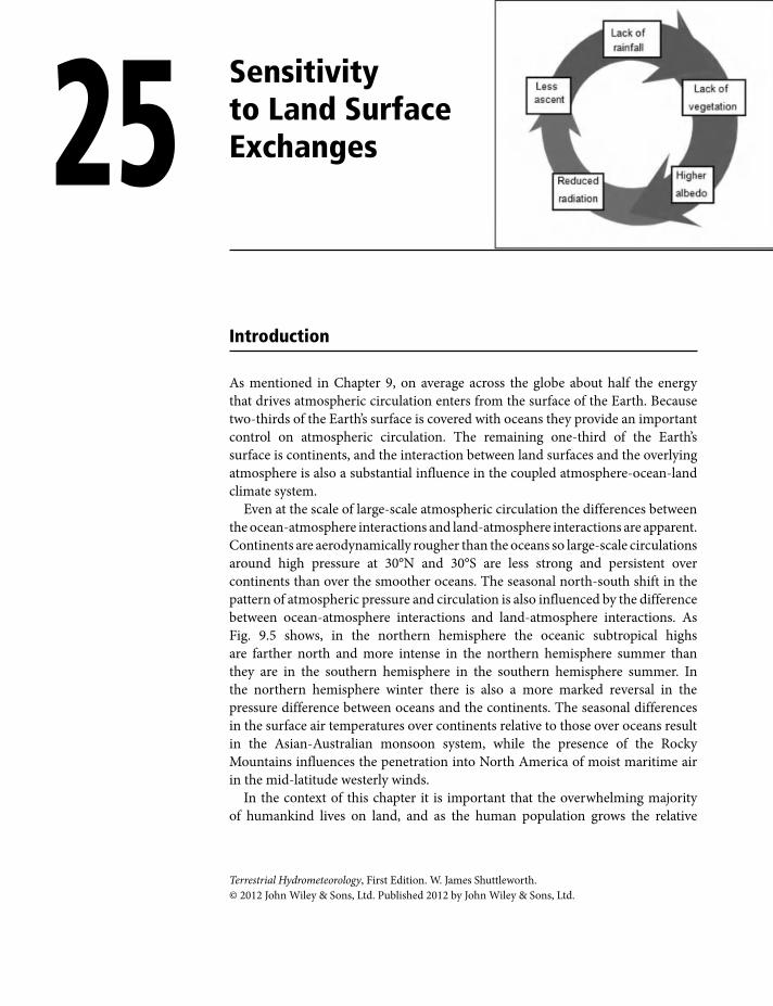
Introduction
As mentioned in Chapter 9, on average across the globe about half the energy
that drives atmospheric circulation enters from the surface of the Earth. Because
two-thirds of the Earth’s surface is covered with oceans they provide an important
control on atmospheric circulation. The remaining one-third of the Earth’s
surface is continents, and the interaction between land surfaces and the overlying
atmosphere is also a substantial influence in the coupled atmosphere-ocean-land
climate system.
Even at the scale of large-scale atmospheric circulation the differences between
the ocean-atmosphere interactions and land-atmosphere interactions are apparent.
Continents are aerodynamically rougher than the oceans so large-scale circulations
around high pressure at 30°N and 30°S are less strong and persistent over
continents than over the smoother oceans. The seasonal north-south shift in the
pattern of atmospheric pressure and circulation is also influenced by the difference
between ocean-atmosphere interactions and land-atmosphere interactions. As
Fig. 9.5 shows, in the northern hemisphere the oceanic subtropical highs
are farther north and more intense in the northern hemisphere summer than
they are in the southern hemisphere in the southern hemisphere summer. In
the northern hemisphere winter there is also a more marked reversal in the
pressure difference between oceans and the continents. The seasonal differences
in the surface air temperatures over continents relative to those over oceans result
in the Asian-Australian monsoon system, while the presence of the Rocky
Mountains influences the penetration into North America of moist maritime air
in the mid-latitude westerly winds.
In the context of this chapter it is important that the overwhelming majority
of humankind lives on land, and as the human population grows the relative
25 Sensitivity to Land Surface Exchanges
Terrestrial Hydrometeorology, First Edition. W. James Shuttleworth.
© 2012 John Wiley & Sons, Ltd. Published 2012 by John Wiley & Sons, Ltd.
Shuttleworth_c25.indd 380Shuttleworth_c25.indd 380 11/3/2011 6:38:33 PM11/3/2011 6:38:33 PM
Atmospheric Sensitivity to Land Surface Exchanges 381
importance of what they do has an increasing influence on climate. The indirect
impact of human activity that results from changing the chemical composition of
the atmosphere is well-recognized and increasingly well-predicted (IPCC, 2007).
However, it is the direct impact of human-induced changes on land surface–
atmosphere exchange processes that concerns us in this chapter. Land surface
exchange processes depend on the nature of the vegetation present, but humans
increasingly change the type of vegetation cover and heterogeneity of land
surfaces, create large urban complexes that replace natural surfaces with artificial
surfaces, and make water more readily available to the atmosphere by irrigating
crops and building dams. As humans do this, the extent to which water, energy,
and momentum is transferred between the atmosphere and the ground
necessarily alters.
In the past, when human population was low, the proportion of the Earth’s land
surfaces that we altered was not large, so its consequence when averaged to the
regional or global scales was less important. But even when conditions higher
in the ABL are little-changed, meteorological variables measured (say) 2 m above
the ground are altered if there is a change in local surface roughness and/or local
surface energy balance (e.g., Bastable et al., 1993). The proportion of land subject
to human influence is already extensive (Fig. 25.1a), and for many of the world’s
important biomes it will continue to increase (Fig. 25.1b) as human population,
which is currently around 6.5 billion, increases by about 50% by the year 2050.
Influence of land surfaces on weather and climate
The available scientific literature on studies of the influence of land surfaces on
weather and climate is large and diverse. To give structure this overview chapter
is divided into three main sub-sections that consider research into, and evidence
for, the influence on weather and climate of (a) existing land-atmosphere interac-
tions; (b) transient changes in land surfaces; and (c) imposed persistent changes
in land cover. When considering influential mechanisms within these three
classifications, in each case we consider first whether the mechanism has a
plausible physical basis. Then we review the evidence that it actually exists by
discussing relevant analyses of weather and climate data (including reanalysis
data), computer model experiments and any other related experimental and
observational studies. This leads to an assessment of the credibility of the
evidence that the mechanism considered is indeed a way in which land surfaces
influence climate and weather using ‘IPCC-like’ categories (IPCC, 2007) of
credibility. Finally we make an assessment of how well this influential mechanism
is currently quantified and represented in models. For convenience these
judgments on the evidence that a particular influential mechanism exists and
the adequacy of our current understanding and modeling of each influence are
tabulated at the end of the chapter. The goal of this table is to give guidance on
priorities by identifying where future research is needed.
Shuttleworth_c25.indd 381Shuttleworth_c25.indd 381 11/3/2011 6:38:34 PM11/3/2011 6:38:34 PM
Cultivated Systems:Areas in which at least30% of the landscapeis cultivated
(a)
MEDITERRANEAN FORESTS,WOODLANDS, AND SCRUB
TEMPERATE FORESTSTEPPE AND WOODLAND
TEMPERATE BROADLEAFAND MIXED FORESTS
TROPICAL ANDSUB-TROPICAL DRY
BROADLEAF FORESTS
FLOODED GRASSLANDSAND SAVANNAS
TROPICAL AND SUB-TROPICALGRASSLANDS, SAVANNAS,
AND SHRUBLANDS
TROPICAL AND SUB-TROPICALCONIFEROUS FORESTS
DESERTS
MONTANE GRASSLANDSAND SHRUBLANDS
TROPICAL AND SUB-TROPICALMOIST BROADLEAF FORESTS
TEMPERATECONIFEROUS FORESTS
BOREALFORESTS
TUNDRA
Conversion of original biomesLoss by1950
Fraction of potential area converted−10 0 10 20 30 40 50 60 70 80 90 100%
Loss between1950 and 1990
Projected lossby 2050*
(b)
Figure 25.1 (a) Land areas which were more than 30% cultivated in 2000. (b) Projected change in original land cover by
2050 given by biome according to the four Millennium Ecosystem scenarios. (Redrawn from MEA, 2005, published with
permission.) See Plate 7 for a colour version of these image.
Shuttleworth_c25.indd 382Shuttleworth_c25.indd 382 11/3/2011 6:38:34 PM11/3/2011 6:38:34 PM
Atmospheric Sensitivity to Land Surface Exchanges 383
A. The influence of existing land-atmosphere interactions
1. Effect of topography on convection and precipitation
Evidence that topography affects weather and climate is irrefutable. When moist
air moving across the Earth encounters topography the resulting orographic flow
gives updrafts and cooling of the air that can generate cloud and so enhance the
probability of rain. Heterogeneous surface heating in mountainous terrain can
also generate mesoscale circulations that impact local atmospheric convection
and result in variations in the spatial distribution of precipitation related to topo-
graphic features such as slope, aspect and elevation. Some effects of topography
can be remote. The atmospheric convection initially generated by topography
can, for example, result in organized mesoscale complexes that give sustained
convective activity that propagates downwind (e.g., Tucker and Crook, 1999).
There is also evidence that topography has a substantial influence on the large-scale
atmospheric circulations involved in the Asian-Australian Monsoon (e.g., Ueda
and Yasunari, 1998). The North American Monsoon Experiment (NAME; Higgins
and Gochis, 2007) is a recent example of an observational study framed around
providing better understanding of monsoon flows including the topographic
influences on precipitation. Figure 25.2 shows the rain gauge transects used
during the NAME and examples of the observed spatial distribution of total
precipitation across the mountainous Sierra Madre Occidental of northwest
Mexico, together with the variation in frequency and maximum intensity of
precipitation as a function of time of day and elevation.
There is a substantial body of literature describing region-specific, observation-
based statistical models of the variations in precipitation (and sometimes
temperature) as a function of location and elevation (e.g., Brown and Comrie,
2002). The quantification of the effect of topography is reasonably good in such
statistical models but they only describe time-average values and, because they are
empirical, they are strictly only relevant in the region in which they are calibrated.
However some, notably the PRISM methodology (Daly et al., 1994; 2008; Johnson
et al., 2000), have been used to extrapolate distributions more generally. There
have been some experimental attempts to understand and describe the influence
of topography on convection using very fine-scale meteorological models (e.g.,
Gopalakrishnan et al., 2000), but the spatial scale of many of the topography-
related processes involved means describing them in mesoscale models operating
at grid-scales of a few kilometers is problematic. Consequently, from the physical
modeling perspective, our present ability to understand and quantify the influence
of topography on weather at the mesoscale remains limited.
Because air temperature falls with height, not only can the amount but also
nature of precipitation change with altitude, especially at mid-latitudes. Much of
the water used by humans originally falls and is often then temporarily stored as
frozen precipitation (Barnett et al., 2005), including most of the water resources of
the western USA for example. The buildup of, and sublimation loss from, snow and
ice in mountainous terrain and the evolution and ultimate melting of snowpack to
Shuttleworth_c25.indd 383Shuttleworth_c25.indd 383 11/3/2011 6:38:35 PM11/3/2011 6:38:35 PM
384 Atmospheric Sensitivity to Land Surface Exchanges
generate hydrological flows remains poorly understood and modeled. Redressing
this shortcoming remains a major challenge for terrestrial hydrometeorology.
Because the physical basis for an influence of topography on weather and
climate is plausible and there is much evidence of its existence in climate records
and from experiments and models, the credibility of this mechanism providing
a means for land surfaces to affect climate and weather is assessed as being
‘extremely likely’ in Table 25.1. Quantification and modeling of the mechanism is
assessed as being of ‘medium’ quality for long-term time averages but is assessed
as still ‘poor’ at short time scales. There is a clear need for more research in this
last area.
0.40
0.35
0.30
0.25
0.20
0.15
Pre
cipi
tatio
n fr
eque
ncy
0.10
0.05
0.000 2 4 6 8 10
Time of day (LST)12 14 16 18 20 22 24
(c)0-500500-10001000-15001500-20002000-25002500-3000Network mean
28 N
24 N
(a)
110 W 106 W
30�00�N
28�00�N
26�00�N
24�00�N
28 N
(b)
24 N
110 W 106 W
30�00�N
28�00�N
26�00�N
24�00�N
10.0
0-5009.0
8.0
7.0
6.0
Pre
cipi
tatio
n in
tens
ity (
mm
/hr)
5.0
4.0
3.0
2.0
1.0
0.00 2 4 6 8 10
Time of day (LST)12 14 16 18 20 22 24
(d)500-10001000-15001500-20002000-25002500-3000Network mean
Figure 25.2 Contours of total precipitation for (a) Aug 2002 and (b) July and Aug 2003 with contour interval 40 mm
derived from the transects of rain gauges located at the positions shown by stars along transects across the Sierra Madre
Mountain Range. Diumal cycles of (c) hourly precipitation frequency and (d) hourly precipitation intensity derived from
these rain gauges separated into elevation-band averages. (Redrawn from Gochis et al., 2004, published with permission.)
Shuttleworth_c25.indd 384Shuttleworth_c25.indd 384 11/3/2011 6:38:35 PM11/3/2011 6:38:35 PM

Atmospheric Sensitivity to Land Surface Exchanges 385
2. Contribution by land surfaces to atmospheric water availability
The hypothesis that land surfaces influence climate and weather by contribut-
ing to the water vapor in the atmosphere is entirely plausible. It requires only
that the amount of water vapor contributed regionally by evaporation from
land surfaces is significant in comparison with that contributed by oceans.
There are now numerous observations and model analyses that indicate the
recycling of water over land surfaces is significant. In fact this significance has
been apparent for decades in global water balance studies (e.g., Baumgartner
and Reichel, 1975; Korzun, 1978) and has been confirmed by more recent
studies (e.g., Oki and Kanae, 2006). As a global average only about 35–45% of
precipitation falling over land leaves as runoff, which implies that the remain-
der is re-evaporated. There is also long-established evidence from global mod-
eling studies (e.g., Shukla and Mintz, 1982) that the atmospheric water vapor
resulting from land surface evaporation has a large effect on modeled
continental precipitation.
Early isotope studies (e.g., Salati et al., 1979) further demonstrated that in
certain areas such as the Amazon River basin about 30% of area-average
precipitation originates from evapotranspiration, and later studies using
reanalysis data sets (e.g. Brubaker et al., 1993; Eltahir and Bras, 1996; Costa and
Foley, 1999; Bosilovich et al., 2005) confirm recycled evaporation accounts for
20–27% of precipitation in this region. The analysis of Makarieva and Gorshkov
(2007) suggests that the efficiency of recycling by forests is greater than for other
land covers so their extensive presence may help maintain precipitation amounts
for greater distances away from coasts. As reanalysis data sets have become
increasingly available there have been numerous studies of atmospheric cycling
including demonstrations of its importance in the context of ecoclimatological
stability (Dominguez and Kumar, 2008) and in monsoon systems (Dominguez
et al., 2008).
Thus, the phenomenon of precipitation recycling is now a well-studied and
well-established facet of terrestrial hydrometeorology and its quantification
and consequences are increasingly well-defined. For this reason in Table 25.1 the
credibility of this mechanism providing the basis of a land surface influence on
climate and weather is assessed as being ‘extremely likely’. But quantification and
modeling of the mechanism is assessed as being of ‘medium’ quality because
further research is justified, with focus on achieving greater realism and accuracy
when modeling surface evaporation and especially the atmospheric mechanisms
involved in releasing precipitation.
B. The influence of transient changes in land surfaces
1. Effect of transient changes in soil moisture
It is physically plausible that moisture stored in the soil which entered from
precipitation can later become re-accessable to the atmosphere, often via plants.
Shuttleworth_c25.indd 385Shuttleworth_c25.indd 385 11/3/2011 6:38:36 PM11/3/2011 6:38:36 PM
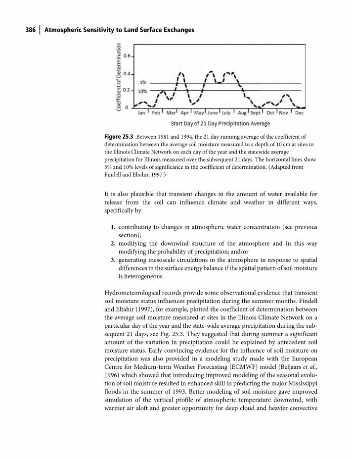
386 Atmospheric Sensitivity to Land Surface Exchanges
It is also plausible that transient changes in the amount of water available for
release from the soil can influence climate and weather in different ways,
specifically by:
1. contributing to changes in atmospheric water concentration (see previous
section);
2. modifying the downwind structure of the atmosphere and in this way
modifying the probability of precipitation; and/or
3. generating mesoscale circulations in the atmosphere in response to spatial
differences in the surface energy balance if the spatial pattern of soil moisture
is heterogeneous.
Hydrometeorological records provide some observational evidence that transient
soil moisture status influences precipitation during the summer months. Findell
and Eltahir (1997), for example, plotted the coefficient of determination between
the average soil moisture measured at sites in the Illinois Climate Network on a
particular day of the year and the state-wide average precipitation during the sub-
sequent 21 days, see Fig. 25.3. They suggested that during summer a significant
amount of the variation in precipitation could be explained by antecedent soil
moisture status. Early convincing evidence for the influence of soil moisture on
precipitation was also provided in a modeling study made with the European
Centre for Medium-term Weather Forecasting (ECMWF) model (Beljaars et al.,
1996) which showed that introducing improved modeling of the seasonal evolu-
tion of soil moisture resulted in enhanced skill in predicting the major Mississippi
floods in the summer of 1993. Better modeling of soil moisture gave improved
simulation of the vertical profile of atmospheric temperature downwind, with
warmer air aloft and greater opportunity for deep cloud and heavier convective
Figure 25.3 Between 1981 and 1994, the 21 day running average of the coefficient of
determination between the average soil moisture measured to a depth of 10 cm at sites in
the Illinois Climate Network on each day of the year and the statewide average
precipitation for Illinois measured over the subsequent 21 days. The horizontal lines show
5% and 10% levels of significance in the coefficient of determination. (Adapted from
Findell and Eltahir, 1997.)
Shuttleworth_c25.indd 386Shuttleworth_c25.indd 386 11/3/2011 6:38:36 PM11/3/2011 6:38:36 PM
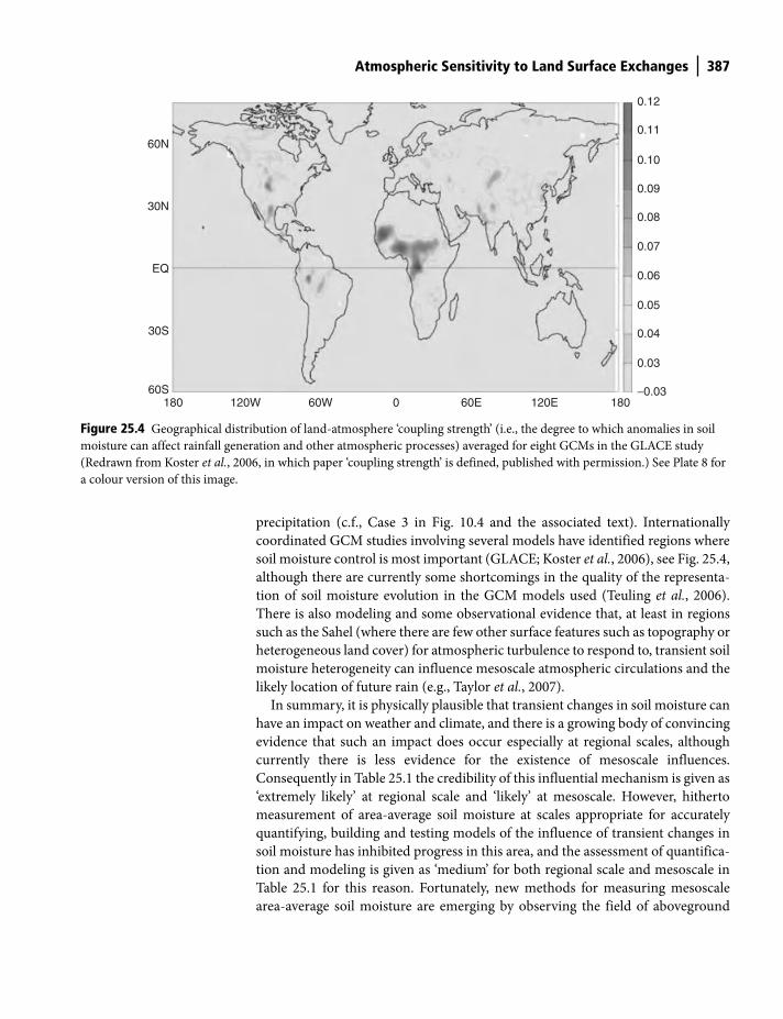
Atmospheric Sensitivity to Land Surface Exchanges 387
precipitation (c.f., Case 3 in Fig. 10.4 and the associated text). Internationally
coordinated GCM studies involving several models have identified regions where
soil moisture control is most important (GLACE; Koster et al., 2006), see Fig. 25.4,
although there are currently some shortcomings in the quality of the representa-
tion of soil moisture evolution in the GCM models used (Teuling et al., 2006).
There is also modeling and some observational evidence that, at least in regions
such as the Sahel (where there are few other surface features such as topography or
heterogeneous land cover) for atmospheric turbulence to respond to, transient soil
moisture heterogeneity can influence mesoscale atmospheric circulations and the
likely location of future rain (e.g., Taylor et al., 2007).
In summary, it is physically plausible that transient changes in soil moisture can
have an impact on weather and climate, and there is a growing body of convincing
evidence that such an impact does occur especially at regional scales, although
currently there is less evidence for the existence of mesoscale influences.
Consequently in Table 25.1 the credibility of this influential mechanism is given as
‘extremely likely’ at regional scale and ‘likely’ at mesoscale. However, hitherto
measurement of area-average soil moisture at scales appropriate for accurately
quantifying, building and testing models of the influence of transient changes in
soil moisture has inhibited progress in this area, and the assessment of quantifica-
tion and modeling is given as ‘medium’ for both regional scale and mesoscale in
Table 25.1 for this reason. Fortunately, new methods for measuring mesoscale
area-average soil moisture are emerging by observing the field of aboveground
60N
30N
EQ
30S
60S180 120W 60W 0 60E 120E 180
−0.03
0.03
0.04
0.05
0.06
0.07
0.08
0.09
0.10
0.11
0.12
Figure 25.4 Geographical distribution of land-atmosphere ‘coupling strength’ (i.e., the degree to which anomalies in soil
moisture can affect rainfall generation and other atmospheric processes) averaged for eight GCMs in the GLACE study
(Redrawn from Koster et al., 2006, in which paper ‘coupling strength’ is defined, published with permission.) See Plate 8 for
a colour version of this image.
Shuttleworth_c25.indd 387Shuttleworth_c25.indd 387 11/3/2011 6:38:36 PM11/3/2011 6:38:36 PM
388 Atmospheric Sensitivity to Land Surface Exchanges
neutrons produced by cosmic rays (Zreda et al., 2008; Shuttleworth et al., 2010), and
at regional scales using satellite systems (Kerr et al., 2001; Entekhabi et al., 2010).
Future research that exploits these new measurement techniques is, therefore,
a priority, and will likely give improved understanding and modeling of this
land-atmosphere feedback mechanism, leading to an assessment of ‘good’.
2. Effect of transient changes in vegetation cover
Because water often leaves soil and enters the atmosphere via transpiration from
plant leaves, the status of the vegetation in terms of leaf cover and plant vigor can
influence the surface energy balance and, through this, weather and climate.
Moreover, living plants can intervene in subterranean flow processes by modifying
soil characteristics or by redistributing water vertically in the soil through the
body of the plant, thus changing the ease and extent to which soil water is
accessible to the atmosphere. The influence of transient changes in vegetation
vigor on weather and climate is therefore physically plausible.
As discussed in detail in Chapter 23, there is long-established evidence of
seasonal changes in evaporation (and therefore in the surface energy balance)
through the growth cycle of annual crops. A common approximate representation
(Allen et al., 1998) has been to assume a seasonal pattern in the crop factor used in
Equation (23.12), see Fig. 23.2. However, most of the evidence for there being
an effect of vegetation cover on climate and weather is derived from modeling
studies, and it takes the form of a simulated difference in model-calculated climate
with and without representation of seasonal changes in leaf area index of the
vegetation covering the ground. The early one-dimensional ‘micrometeorological’
land surface models (e.g., Dickinson et al., 1986; Sellers et al., 1986) used in GCMs
(see Chapter 24 for description) took it as self-evident that transient changes in
vegetation cover will influence climate, and they had seasonal variations in the leaf
area index of the vegetation prescribed using look-up tables to accommodate
this. More recently (again see Chapter 24) SVATS have emerged with improved
representation of carbon dioxide exchange (e.g., Sellers et al., 1996; Dickinson
et al., 1998; Cox et al., 1998) and this allows simulation of seasonal changes in
simulated leaf area index of vegetation through the year. Such SVATS are some-
times referred to as having interactive vegetation. Incorporating interactive
vegetation can result in significant changes in the modeled surface evaporation
and precipitation, see Fig. 25.5. Because remote sensing can be used to provide an
indirect estimate of the amount and vigor of vegetation (see Fig. 5.6 and associated
text), some modeling studies have also considered the effect of introducing
remotely sensed estimates of changing vegetation on modeled climate and
have found that doing so can give significant effects (e.g., Matsui et al., 2005).
It is widely accepted among the scientific community that transient (generally
seasonal) changes in vegetation cover will affect weather and climate and,
consistent with this, this influential mechanism is assessed as being ‘extremely
likely’ in Table 25.1. Motivated by a desire to include the feedback effects of
vegetation change in response to atmospheric carbon dioxide concentration, over
Shuttleworth_c25.indd 388Shuttleworth_c25.indd 388 11/3/2011 6:38:37 PM11/3/2011 6:38:37 PM
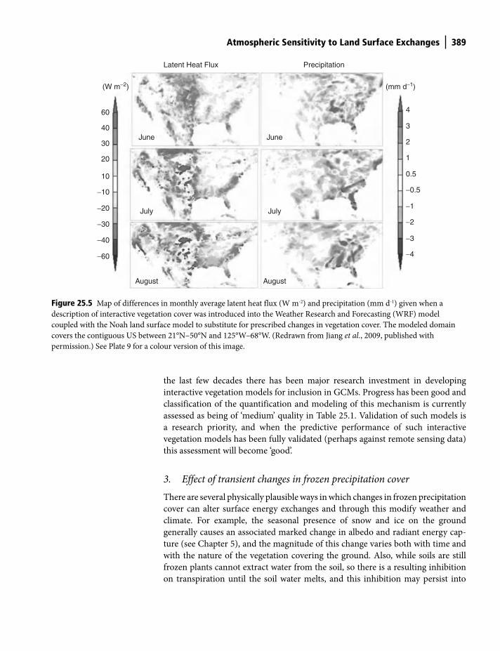
Atmospheric Sensitivity to Land Surface Exchanges 389
the last few decades there has been major research investment in developing
interactive vegetation models for inclusion in GCMs. Progress has been good and
classification of the quantification and modeling of this mechanism is currently
assessed as being of ‘medium’ quality in Table 25.1. Validation of such models is
a research priority, and when the predictive performance of such interactive
vegetation models has been fully validated (perhaps against remote sensing data)
this assessment will become ‘good’.
3. Effect of transient changes in frozen precipitation cover
There are several physically plausible ways in which changes in frozen precipitation
cover can alter surface energy exchanges and through this modify weather and
climate. For example, the seasonal presence of snow and ice on the ground
generally causes an associated marked change in albedo and radiant energy cap-
ture (see Chapter 5), and the magnitude of this change varies both with time and
with the nature of the vegetation covering the ground. Also, while soils are still
frozen plants cannot extract water from the soil, so there is a resulting inhibition
on transpiration until the soil water melts, and this inhibition may persist into
60
(W m−2) (mm d−1)
4
3
2
1
0.5
−0.5
−1
−2
−3
−4
June June
Latent Heat Flux Precipitation
July July
August August
40
30
20
10
−10
−20
−30
−40
−60
Figure 25.5 Map of differences in monthly average latent heat flux (W m-2) and precipitation (mm d-1) given when a
description of interactive vegetation cover was introduced into the Weather Research and Forecasting (WRF) model
coupled with the Noah land surface model to substitute for prescribed changes in vegetation cover. The modeled domain
covers the contiguous US between 21°N–50°N and 125°W–68°W. (Redrawn from Jiang et al., 2009, published with
permission.) See Plate 9 for a colour version of this image.
Shuttleworth_c25.indd 389Shuttleworth_c25.indd 389 11/3/2011 6:38:37 PM11/3/2011 6:38:37 PM
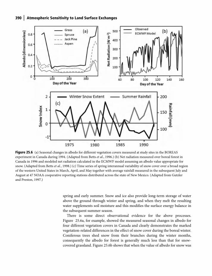
390 Atmospheric Sensitivity to Land Surface Exchanges
spring and early summer. Snow and ice also provide long-term storage of water
above the ground through winter and spring, and when they melt the resulting
water supplements soil moisture and this modifies the surface energy balance in
the subsequent summer season.
There is some direct observational evidence for the above processes.
Figure 25.6a, for example, showed the measured seasonal changes in albedo for
four different vegetation covers in Canada and clearly demonstrates the marked
vegetation-related differences in the effect of snow cover during the boreal winter.
Coniferous trees shed snow from their branches during the winter months,
consequently the albedo for forest is generally much less than that for snow-
covered grassland. Figure 25.6b shows that when the value of albedo for snow was
Figure 25.6 (a) Seasonal changes in albedo for different vegetation covers measured at study sites in the BOREAS
experiment in Canada during 1994. (Adapted from Betts et al., 1996.) (b) Net radiation measured over boreal forest in
Canada in 1996 and modeled net radiation calculated in the ECMWF model assuming an albedo value appropriate for
snow. (Adapted from Betts et al., 1998.) (c) Time series of spring interannual variability of snow cover over a broad region
of the western United States in March, April, and May together with average rainfall measured in the subsequent July and
August at 47 NOAA cooperative reporting stations distributed across the state of New Mexico. (Adapted from Gutzler
and Preston, 1997.)
Shuttleworth_c25.indd 390Shuttleworth_c25.indd 390 11/3/2011 6:38:37 PM11/3/2011 6:38:37 PM
Atmospheric Sensitivity to Land Surface Exchanges 391
(wrongly) assigned to the boreal forest in Canada during the snow-covered winter
months in the ECMWF model it calculated values of net radiation that were
substantially less than observed values. Figure 25.6c shows that the snow cover
over a broad region of the western United States in March, April, and May appears
to be anti-correlated with area-average monsoon rainfall measured in the
subsequent July and August in New Mexico, a feature which has been ascribed
to the effect of snow melt on summer soil moisture.
Because the influences of transient changes in frozen precipitation cover are
physically plausible and consistent with observations, this influential mechanism
is assessed as being ‘extremely likely’ in Table 25.1. Over the last decade there has
been significant effort deployed toward improving the representation of frozen
precipitation in SVATS (e.g., Bowling et al., 2003; Luo et al., 2003; Nijssen et al.,
2003; Etchevers et al., 2004; Niu and Yang, 2004; 2006; 2007; Fassnacht et al.,
2006). Because progress has been reasonably good, the classification of the
quantification and modeling of this mechanism is currently assessed as being of
‘medium’ quality in Table 25.1. Adequate representation of area-average behavior
of heterogeneous frozen precipitation cover and its influence on meteorological
feedbacks and hydrological flows remains elusive and merits further research.
4. Combined effect of transient changes
For simplicity and clarity the mechanisms through which land surfaces can
influence climate and weather associated with soil moisture, vegetation cover and
frozen precipitation have been considered separately above. But it is important to
recognize that in practice they are intimately interrelated. This is true in the real
world and should also be true in any well-conceived model of surface processes.
The atmosphere’s ability to access soil moisture is related to vegetation cover
because plants’ roots, stems and leaves serve as an important conduit between
soil and the overlying air. Plants can also intercept precipitation and return it to
the atmosphere before it enters the soil, thus changing the amount of moisture
present in the soil that is available to the atmosphere. Coverings of snow and ice
and associated frozen soil influence the effect of vegetation cover by altering
surface albedo and by inhibiting transpiration from plants when soil is frozen.
Water temporarily stored in frozen form on the surface of soil and vegetation
during winter usually melts several months later and supplements the soil mois-
ture available to transpiring vegetation in the subsequent summer. The evolution
of the snow cover with time depends on what vegetation is present because tall
forests may shade snow, while snow on short grassland remains exposed to the
sun. Similarly, the seasonal cycle in vegetation growth and the extent to which
plants’ controls act to moderate transpiration rate are related to the amount of
moisture in the soil.
Because of the complexity of the regional scale interaction between the
three influential mechanisms associated with soil moisture, vegetation cover
and frozen precipitation, it is perhaps not surprising that all are assessed as
‘extremely likely’ in Table 25.1, and that the present status of understanding and
Shuttleworth_c25.indd 391Shuttleworth_c25.indd 391 11/3/2011 6:38:38 PM11/3/2011 6:38:38 PM
392 Atmospheric Sensitivity to Land Surface Exchanges
modeling these mechanisms are all assessed as ‘medium’. In practice it is likely
that future improvements in understanding and modeling will most effectively
be made by comprehensive studies in which models are challenged using a suite
of sustained observations made over several seasons that includes measure-
ments of the variables associated with all three of these influential mechanisms
simultaneously.
C. The influence of imposed persistent changes in land cover
As mentioned earlier in this chapter, the land cover and hydrological behavior of
large areas of the globe have now been altered greatly by human intervention and
continued changes seem inevitable as human population continues to grow.
Because land surface exchange helps determine how the overlying atmosphere
behaves, persistent changes in the nature of land surfaces inevitably have an effect
on weather and climate. Small-scale changes have some effect on weather variables
that are measured near the ground (typically at 2 m) because local surface
influences in part determine these. Larger regional-scale changes in land surface
features can have influence higher in the atmosphere and give rise to regional
or even global scale modifications to atmospheric processes and flows. Such
modifications arise in two main ways, either because the area-average surface
exchanges are modified over a large area, or because development introduces
heterogeneity into land surface exchanges at a spatial scale such as to generate
mesoscale circulations in the atmosphere that may alter the probability and
whereabouts of cloud and precipitation. For simplicity, the influence of persistent
changes in land cover are considered separately below, although in practice all
three influences may well act simultaneously.
1. Effect of imposed land cover change on near surface observations
The values of climate variables measured at (say) 2 m above the ground depend on
vertical profiles that are determined by the land-cover dependent turbulent
transfer of energy, water and momentum fluxes between the surface and the mixed
layer in the Atmospheric Boundary Layer (see Chapter 19 and Fig. 19.6). This fact
is recognized explicitly in the derivation of the Matt-Shuttleworth approach
(Shuttleworth, 2006; Shuttleworth and Wallace, 2009), see the relevant section
in Chapter 23. Observed differences in near-surface climate are easily observed
and have, for example, been reported over small clearings and natural forest in
Amazonia (Figs 25.7a,b,c), and in the form of the ‘urban heat island’ phenomenon
when regions undergo extensive urbanization (Fig. 25.7d).
Because the changes in near-surface climate that are associated with imposed
land cover change are readily understood in terms of present day turbulent
transport theory and are readily observed, the assessment of likelihood for
this influential mechanism is assessed as ‘extremely likely’, and the level of
understanding and modeling as ‘good’ in Table 25.1.
Shuttleworth_c25.indd 392Shuttleworth_c25.indd 392 11/3/2011 6:38:38 PM11/3/2011 6:38:38 PM
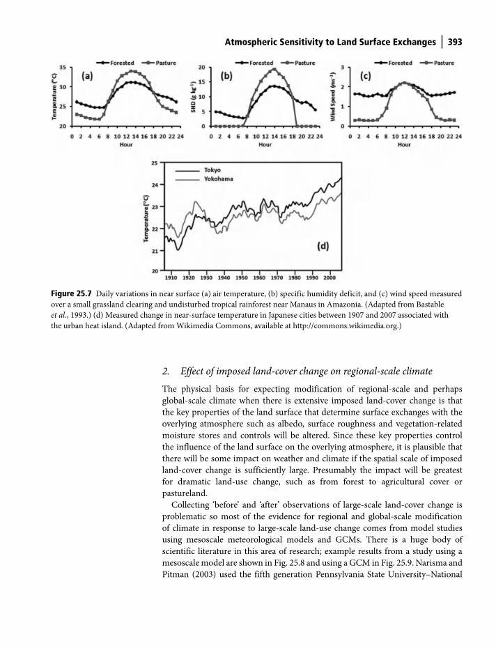
Atmospheric Sensitivity to Land Surface Exchanges 393
2. Effect of imposed land-cover change on regional-scale climate
The physical basis for expecting modification of regional-scale and perhaps
global-scale climate when there is extensive imposed land-cover change is that
the key properties of the land surface that determine surface exchanges with the
overlying atmosphere such as albedo, surface roughness and vegetation-related
moisture stores and controls will be altered. Since these key properties control
the influence of the land surface on the overlying atmosphere, it is plausible that
there will be some impact on weather and climate if the spatial scale of imposed
land-cover change is sufficiently large. Presumably the impact will be greatest
for dramatic land-use change, such as from forest to agricultural cover or
pastureland.
Collecting ‘before’ and ‘after’ observations of large-scale land-cover change is
problematic so most of the evidence for regional and global-scale modification
of climate in response to large-scale land-use change comes from model studies
using mesoscale meteorological models and GCMs. There is a huge body of
scientific literature in this area of research; example results from a study using a
mesoscale model are shown in Fig. 25.8 and using a GCM in Fig. 25.9. Narisma and
Pitman (2003) used the fifth generation Pennsylvania State University–National
Figure 25.7 Daily variations in near surface (a) air temperature, (b) specific humidity deficit, and (c) wind speed measured
over a small grassland clearing and undisturbed tropical rainforest near Manaus in Amazonia. (Adapted from Bastable
et al., 1993.) (d) Measured change in near-surface temperature in Japanese cities between 1907 and 2007 associated with
the urban heat island. (Adapted from Wikimedia Commons, available at http://commons.wikimedia.org.)
Shuttleworth_c25.indd 393Shuttleworth_c25.indd 393 11/3/2011 6:38:38 PM11/3/2011 6:38:38 PM
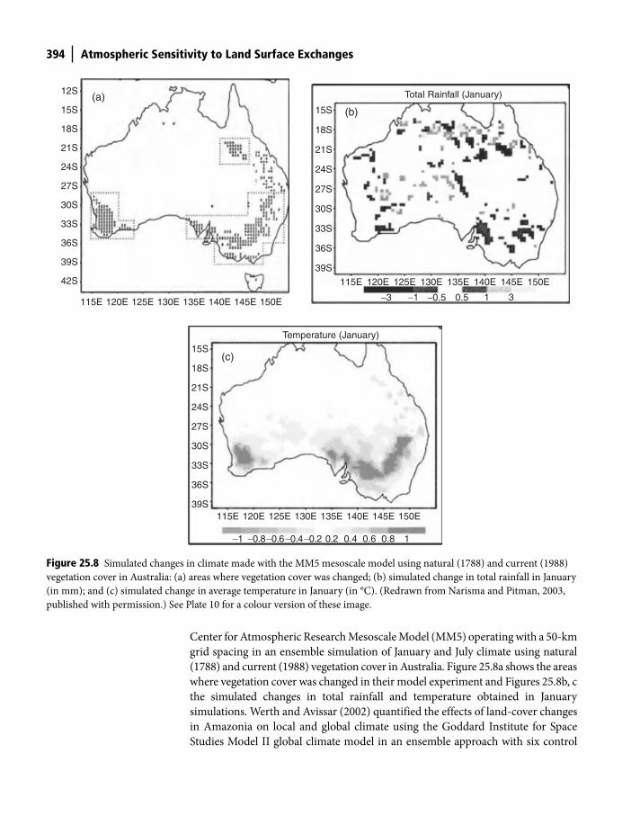
394 Atmospheric Sensitivity to Land Surface Exchanges
Center for Atmospheric Research Mesoscale Model (MM5) operating with a 50-km
grid spacing in an ensemble simulation of January and July climate using natural
(1788) and current (1988) vegetation cover in Australia. Figure 25.8a shows the areas
where vegetation cover was changed in their model experiment and Figures 25.8b, c
the simulated changes in total rainfall and temperature obtained in January
simulations. Werth and Avissar (2002) quantified the effects of land-cover changes
in Amazonia on local and global climate using the Goddard Institute for Space
Studies Model II global climate model in an ensemble approach with six control
Temperature (January)
(c)
−1 −0.8−0.6−0.4−0.2 0.2 0.4 0.6 0.8 1
115E39S
36S
33S
30S
27S
24S
21S
18S
15S
120E 125E 130E 135E 140E 145E 150E
(a)
42S
39S
36S
33S
30S
27S
24S
21S
18S
15S
12S
115E 120E 125E 130E 135E 140E 145E 150E −3 −1 1 3−0.5 0.5
(b)
39S
36S
33S
30S
27S
24S
21S
18S
15S
115E 120E 125E 130E 135E 140E 145E 150E
Total Rainfall (January)
Figure 25.8 Simulated changes in climate made with the MM5 mesoscale model using natural (1788) and current (1988)
vegetation cover in Australia: (a) areas where vegetation cover was changed; (b) simulated change in total rainfall in January
(in mm); and (c) simulated change in average temperature in January (in °C). (Redrawn from Narisma and Pitman, 2003,
published with permission.) See Plate 10 for a colour version of these image.
Shuttleworth_c25.indd 394Shuttleworth_c25.indd 394 11/3/2011 6:38:38 PM11/3/2011 6:38:38 PM
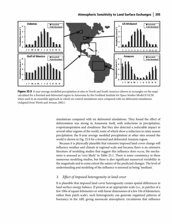
Atmospheric Sensitivity to Land Surface Exchanges 395
simulations compared with six deforested simulations. They found the effect of
deforestation was strong in Amazonia itself, with reductions in precipitation,
evapotranspiration and cloudiness. But they also detected a noticeable impact in
several other regions of the world, some of which show a reduction in rainy season
precipitation: the 8-year average modeled precipitation at other sites around the
world is shown in Fig. 25.9 for a forested and deforested Amazon region.
Because it is physically plausible that extensive imposed land-cover change will
influence weather and climate at regional scale and because there is an extensive
literature of modeling studies that suggest this influence does occur, the mecha-
nism is assessed as ‘very likely’ in Table 25.1. There is some consistency in these
numerous modeling studies, but there is also significant numerical variability in
the magnitude and to some extent the nature of the predicted changes. The level of
understanding and modeling of the influence is assessed as being ‘medium’.
3. Effect of imposed heterogeneity in land cover
It is plausible that imposed land-cover heterogeneity creates spatial differences in
land surface energy balance. If present at an appropriate scale (i.e., in patches of a
few 100s of square kilometers or with linear dimensions of a few 10s of kilometers,
rather than patch-scale), such heterogeneity can generate organized patterns of
buoyancy in the ABL giving mesoscale atmospheric circulations that influence
Figure 25.9 8-year average modelled precipitation at sites in North and South America (shown as rectangles on the map)
calculated for a forested and deforested region in Amazonia by the Goddard Institute for Space Studies Model II GCM
when used in an ensemble approach in which six control simulations were compared with six deforested simulations.
(Adapted from Werth and Avissar, 2002.)
Shuttleworth_c25.indd 395Shuttleworth_c25.indd 395 11/3/2011 6:38:39 PM11/3/2011 6:38:39 PM
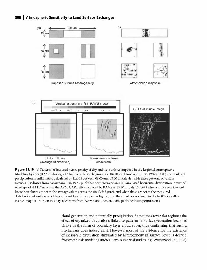
396 Atmospheric Sensitivity to Land Surface Exchanges
cloud generation and potentially precipitation. Sometimes (over flat regions) the
effect of organized circulations linked to patterns in surface vegetation becomes
visible in the form of boundary layer cloud cover, thus confirming that such a
mechanism does indeed exist. However, most of the evidence for the existence
of mesoscale circulation stimulated by heterogeneity in surface cover is derived
from mesoscale modeling studies. Early numerical studies (e.g., Avissar and Liu, 1996)
Uniform fluxes(average of observed)
Heterogeneous fluxes(observed)
Vertical ascent (m s−1) in RAMS model
GOES-8 Visible Image
Atmospheric responseImposed surface heterogeneity
60 km(a)
(c)
(b)
30 km
30 km
15 km
−0.25 0 0.25 0.75 1 1.25 1.50.5
Figure 25.10 (a) Patterns of imposed heterogeneity of dry and wet surfaces imposed in the Regional Atmospheric
Modeling System (RAMS) during a 12 hour simulation beginning at 06:00 local time on July 28, 1989 and (b) accumulated
precipitation in millimeters calculated by RAMS between 06:00 and 18:00 on this day with these patterns of surface
wetness. (Redrawn from Avissar and Liu, 1996, published with permission.) (c) Simulated horizontal distribution in vertical
wind speed at 1117 m across the ARM-CART site calculated by RAMS at 15:30 on July 13, 1995 when surface sensible and
latent heat fluxes are set to the average values across the site (left figure), and when these are set to the measured
distribution of surface sensible and latent heat fluxes (center figure), and the cloud cover shown in the GOES-8 satellite
visible image at 15:15 on this day. (Redrawn from Weaver and Avissar, 2001, published with permission.)
Shuttleworth_c25.indd 396Shuttleworth_c25.indd 396 11/3/2011 6:38:39 PM11/3/2011 6:38:39 PM

Tabl
e 25
.1 A
sses
smen
t o
f th
e cr
edib
ilit
y th
at s
pec
ifie
d l
and
-atm
osp
her
e co
up
lin
g m
ech
anis
ms
act
to i
nfl
uen
ce w
eath
er a
nd
cli
mat
e m
ade
on
th
e b
asis
of
ph
ysic
al p
lau
sib
ilit
y an
d t
he
avai
lab
ilit
y o
f o
bse
rvat
ion
al a
nd
mo
del
ing
evid
ence
(o
verv
iew
ed i
n t
he
text
) to
geth
er w
ith
an
ass
essm
ent
of
the
curr
ent
leve
l of
un
der
stan
din
g o
f ea
ch m
ech
anis
m a
nd
pre
sen
t d
ay a
bil
ity
to r
epre
sen
t it
in
mo
del
s.
Land
-sur
face
infl
uenc
e on
clim
ate
or w
eath
er
Plau
sibl
e ph
ysic
al b
asis
fo
r th
e in
flue
nce
Obs
erva
tion
al
evid
ence
for
th
e in
flue
nce
Mod
elin
g ev
iden
ce
for
the
infl
uenc
e
Cred
ibili
ty
of in
flue
ntia
l m
echa
nism
*
Qua
ntif
icat
ion
and
mod
elin
g of
infl
uenc
e (G
ood,
Med
ium
, or
Poo
r)
A.
Infl
uen
ce o
f ex
isti
ng
la
nd
-atm
osp
her
e in
tera
ctio
ns
1. I
nflu
ence
of t
opog
raph
yYe
sYe
sYe
sEx
trem
ely
likel
yLo
ng-t
erm
: Med
ium
2. C
ontr
ibut
ion
to a
tmos
pher
ic w
ater
av
aila
bilit
y (“
recy
clin
g”)
Yes
Yes
Yes
Extr
emel
y lik
ely
Shor
t-te
rm: P
oor
Med
ium
B.
Infl
uen
ce o
f tr
ansi
ent
chan
ges
in
lan
d s
urf
aces
1. T
rans
ient
cha
nges
in s
oil m
oist
ure:
a.
Reg
iona
l sca
le in
fluen
ce o
n cl
imat
eYe
sYe
sYe
sEx
trem
ely
likel
yM
ediu
m
b.
Mes
osca
le in
fluen
ce o
n w
eath
erYe
sYe
sYe
sLi
kely
Med
ium
2. T
rans
ient
cha
nges
in v
eget
atio
nYe
sYe
sYe
sEx
trem
ely
likel
yM
ediu
m3.
Tra
nsie
nt c
hang
es in
froz
en p
reci
pita
tion
cove
rYe
sYe
sYe
sEx
trem
ely
likel
yM
ediu
m
(N
ote:
in p
ract
ice
thes
e in
fluen
ces
are
stro
ngly
cou
pled
)C
. In
flu
ence
of
imp
ose
d c
han
ges
in
lan
d c
ove
r1.
Loc
al e
ffect
on
2 m
clim
ate
Yes
Yes
Yes
Extr
emel
y lik
ely
Goo
d2.
Effe
ct o
f reg
iona
l-sca
le c
hang
es
in la
nd c
over
Yes
Som
eYe
sVe
ry li
kely
Med
ium
3. E
ffect
of i
mpo
sed
land
-cov
er
hete
roge
neity
Ye
s
Yes
Ye
s
Extr
emel
y lik
ely
Med
ium
* Ex
trem
ely
likel
y >
95%
; Ver
y lik
ely
> 9
0%; L
ikel
y >
66%
; Mor
e lik
ely
than
not
> 5
0%; U
nlik
ely
< 3
3%; V
ery
Unl
ikel
y <
10%
; Ext
rem
ely
unlik
ely
< 5
%
Shuttleworth_c25.indd 397Shuttleworth_c25.indd 397 11/3/2011 6:38:40 PM11/3/2011 6:38:40 PM
398 Atmospheric Sensitivity to Land Surface Exchanges
investigated the phenomenon with artificially imposed patterns of surface heating
and demonstrated modeled mesoscale circulation linked to precipitation, see
Fig. 25.10. Later studies (e.g., Weaver and Avissar, 2001) sought validation of such
circulations and their consequences with reference to observations, see Fig. 25.10.
Some attempts have been made to parameterize the effect of land surface hetero-
geneity on ABL turbulence (e.g., Liu et al., 1999) but, at this writing, this is rarely
if ever done in GCMs, perhaps because other surface features such as topography
and soil moisture heterogeneity can also give rise to mesoscale circulations.
Given the plausibility that mesoscale circulations will arise in response to land
surface heterogeneity circulations, and that these can be simulated in mesoscale
meteorological models and associated boundary layer cloud patterns have some-
times been observed, this mechanism is considered ‘extremely likely’ in Table 25.1.
Assessing the level of understanding and modeling of this influential mechanism
is complicated by the fact that the phenomenon is readily represented in mes-
oscale meteorological models suggesting an assessment of ‘good’, but they are not
yet represented in GCMs suggesting an assessment of ‘poor’. As a compromise, in
Table 25.1 the assessment given is ‘medium’.
Important points in this chapter
● Land surfaces do matter: because a continental influence is evident in
global-scale atmospheric general circulation, see Chapter 9.
● Review: a critical review of the available literature in three general areas,
i.e.,(a) the influence of existing land-atmosphere interactions; (b) the
influence of transient changes in land surfaces; and (c) the influence of
imposed persistent changes in land cover indicates the following conclusions
which are summarized in Table 25.1:
— The credibility of all the land surface influences on the atmosphere
considered is assessed as being ‘extremely likely’ or ‘very likely’, except
in one case when it is considered ‘likely’.
— Present ability to quantify the magnitude and model all these
influences is assessed as ‘medium’, except in one case it is assessed as
‘high’ and in one case as ‘poor’.
— The influence of soil moisture, vegetation cover, and frozen
precipitation cannot be separately modeled. Future improvements will
most effectively be made by studies in which sustained observations
are made over several seasons and include measurements associated
with all three of these influential mechanisms simultaneously.
● Recommendations: areas that priorities in future research are as follows:
— Quantification and modeling of the effect of topography on weather
and climate at short time scales is assessed as being poor and there is a
clear need for more research in this area.
Shuttleworth_c25.indd 398Shuttleworth_c25.indd 398 11/3/2011 6:38:40 PM11/3/2011 6:38:40 PM
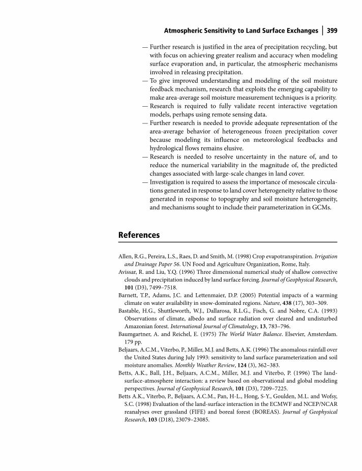
Atmospheric Sensitivity to Land Surface Exchanges 399
— Further research is justified in the area of precipitation recycling, but
with focus on achieving greater realism and accuracy when modeling
surface evaporation and, in particular, the atmospheric mechanisms
involved in releasing precipitation.
— To give improved understanding and modeling of the soil moisture
feedback mechanism, research that exploits the emerging capability to
make area-average soil moisture measurement techniques is a priority.
— Research is required to fully validate recent interactive vegetation
models, perhaps using remote sensing data.
— Further research is needed to provide adequate representation of the
area-average behavior of heterogeneous frozen precipitation cover
because modeling its influence on meteorological feedbacks and
hydrological flows remains elusive.
— Research is needed to resolve uncertainty in the nature of, and to
reduce the numerical variability in the magnitude of, the predicted
changes associated with large-scale changes in land cover.
— Investigation is required to assess the importance of mesoscale circula-
tions generated in response to land cover heterogeneity relative to those
generated in response to topography and soil moisture heterogeneity,
and mechanisms sought to include their parameterization in GCMs.
References
Allen, R.G., Pereira, L.S., Raes, D. and Smith, M. (1998) Crop evapotranspiration. Irrigation
and Drainage Paper 56. UN Food and Agriculture Organization, Rome, Italy.
Avissar, R. and Liu, Y.Q. (1996) Three dimensional numerical study of shallow convective
clouds and precipitation induced by land surface forcing. Journal of Geophysical Research,
101 (D3), 7499–7518.
Barnett, T.P., Adams, J.C. and Lettenmaier, D.P. (2005) Potential impacts of a warming
climate on water availability in snow-dominated regions. Nature, 438 (17), 303–309.
Bastable, H.G., Shuttleworth, W.J., Dallarosa, R.L.G., Fisch, G. and Nobre, C.A. (1993)
Observations of climate, albedo and surface radiation over cleared and undisturbed
Amazonian forest. International Journal of Climatology, 13, 783–796.
Baumgartner, A. and Reichel, E. (1975) The World Water Balance. Elsevier, Amsterdam.
179 pp.
Beljaars, A.C.M., Viterbo, P., Miller, M.J. and Betts, A.K. (1996) The anomalous rainfall over
the United States during July 1993: sensitivity to land surface parameterization and soil
moisture anomalies. Monthly Weather Review, 124 (3), 362–383.
Betts, A.K., Ball, J.H., Beljaars, A.C.M., Miller, M.J. and Viterbo, P. (1996) The land-
surface-atmosphere interaction: a review based on observational and global modeling
perspectives. Journal of Geophysical Research, 101 (D3), 7209–7225.
Betts A.K., Viterbo, P., Beljaars, A.C.M., Pan, H-L., Hong, S-Y., Goulden, M.L. and Wofsy,
S.C. (1998) Evaluation of the land-surface interaction in the ECMWF and NCEP/NCAR
reanalyses over grassland (FIFE) and boreal forest (BOREAS). Journal of Geophysical
Research, 103 (D18), 23079–23085.
Shuttleworth_c25.indd 399Shuttleworth_c25.indd 399 11/3/2011 6:38:40 PM11/3/2011 6:38:40 PM
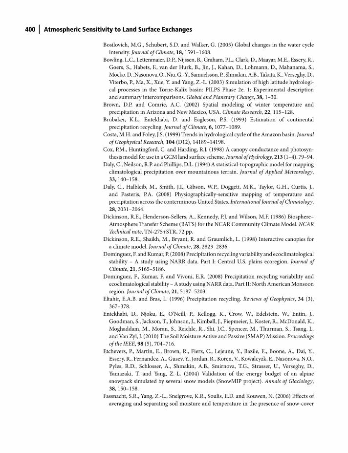
400 Atmospheric Sensitivity to Land Surface Exchanges
Bosilovich, M.G., Schubert, S.D. and Walker, G. (2005) Global changes in the water cycle
intensity. Journal of Climate, 18, 1591–1608.
Bowling, L.C., Lettenmaier, D.P., Nijssen, B., Graham, P.L., Clark, D., Maayar, M.E., Essery, R.,
Goers, S., Habets, F., van der Hurk, B., Jin, J., Kahan, D., Lohmann, D., Mahanama, S.,
Mocko, D., Nasonova, O., Niu, G.-Y., Samuelsson, P., Shmakin, A.B., Takata, K., Verseghy, D.,
Viterbo, P., Ma, X., Xue, Y. and Yang, Z.-L. (2003) Simulation of high latitude hydrologi-
cal processes in the Torne-Kalix basin: PILPS Phase 2e. 1: Experimental description
and summary intercomparisons. Global and Planetary Change, 38, 1–30.
Brown, D.P. and Comrie, A.C. (2002) Spatial modeling of winter temperature and
precipitation in Arizona and New Mexico, USA. Climate Research, 22, 115–128.
Brubaker, K.L., Entekhabi, D. and Eagleson, P.S. (1993) Estimation of continental
precipitation recycling. Journal of Climate, 6, 1077–1089.
Costa, M.H. and Foley, J.S. (1999) Trends in hydrological cycle of the Amazon basin. Journal
of Geophysical Research, 104 (D12), 14189–14198.
Cox, P.M., Huntingford, C. and Harding, R.J. (1998) A canopy conductance and photosyn-
thesis model for use in a GCM land surface scheme. Journal of Hydrology, 213 (1–4), 79–94.
Daly, C., Neilson, R.P. and Phillips, D.L. (1994) A statistical-topographic model for mapping
climatological precipitation over mountainous terrain. Journal of Applied Meteorology,
33, 140–158.
Daly, C., Halbleib, M., Smith, J.I., Gibson, W.P., Doggett, M.K., Taylor, G.H., Curtis, J.,
and Pasteris, P.A. (2008) Physiographically-sensitive mapping of temperature and
precipitation across the conterminous United States. International Journal of Climatology,
28, 2031–2064.
Dickinson, R.E., Henderson-Sellers, A., Kennedy, P.J. and Wilson, M.F. (1986) Biosphere–
Atmosphere Transfer Scheme (BATS) for the NCAR Community Climate Model. NCAR
Technical note, TN-275+STR, 72 pp.
Dickinson, R.E., Shaikh, M., Bryant, R. and Graumlich, L. (1998) Interactive canopies for
a climate model. Journal of Climate, 28, 2823–2836.
Dominguez, F. and Kumar, P. (2008) Precipitation recycling variability and ecoclimatological
stability – A study using NARR data. Part I: Central U.S. plains ecoregion. Journal of
Climate, 21, 5165–5186.
Dominguez, F., Kumar, P. and Vivoni, E.R. (2008) Precipitation recycling variability and
ecoclimatological stability – A study using NARR data. Part II: North American Monsoon
region. Journal of Climate, 21, 5187–5203.
Eltahir, E.A.B. and Bras, L. (1996) Precipitation recycling. Reviews of Geophysics, 34 (3),
367–378.
Entekhabi, D., Njoku, E., O’Neill, P., Kellogg, K., Crow, W., Edelstein, W., Entin, J.,
Goodman, S., Jackson, T., Johnson, J., Kimball, J., Piepmeier, J., Koster, R., McDonald, K.,
Moghaddam, M., Moran, S., Reichle, R., Shi, J.C., Spencer, M., Thurman, S., Tsang, L.
and Van Zyl, J. (2010) The Soil Moisture Active and Passive (SMAP) Mission. Proceedings
of the IEEE, 98 (5), 704–716.
Etchevers, P., Martin, E., Brown, R., Fierz, C., Lejeune, Y., Bazile, E., Boone, A., Dai, Y.,
Essery, R., Fernandez, A., Gusev, Y., Jordan, R., Koren, V., Kowalcyzk, E., Nasonova, N.O.,
Pyles, R.D., Schlosser, A., Shmakin, A.B., Smirnova, T.G., Strasser, U., Verseghy, D.,
Yamazaki, T. and Yang, Z.-L. (2004) Validation of the energy budget of an alpine
snowpack simulated by several snow models (SnowMIP project). Annals of Glaciology,
38, 150–158.
Fassnacht, S.R., Yang, Z.-L., Snelgrove, K.R., Soulis, E.D. and Kouwen, N. (2006) Effects of
averaging and separating soil moisture and temperature in the presence of snow-cover
Shuttleworth_c25.indd 400Shuttleworth_c25.indd 400 11/3/2011 6:38:40 PM11/3/2011 6:38:40 PM
Atmospheric Sensitivity to Land Surface Exchanges 401
in a SVAT and hydrological model for a southern Ontario, Canada, watershed. Journal
of Hydrometeorology, 7, 298–304.
Findell, K.L. and Eltahir, E.A. (1997) An analysis of the soil moisture–rainfall feedback,
based on direct observations from Illinois. Water Resources Research,. 33, 725–735.
Gochis, D.J., Jimenez, A., Watts, C.J., Garatuza-Payan, J. and Shuttleworth, W.J. (2004)
Analysis of 2002 and 2003 warm-season precipitation from the North American monsoon
experiment event rain gauge network. Monthly Weather Review, 132, 2938–2953.
Gopalakrishnan, S.G., Roy, S.B. and Avissar, R. (2000) An evaluation of the scale at
which topographical features affect the convective boundary layer using large eddy
simulations. Journal of the Atmospheric Sciences, 57, 334–351.
Gutzler, D. and Preston, J. (1997) Evidence for a relationship between spring snow cover in
North America and summer rainfall in New Mexico. Geophysical Research Letters, 24,
2207–2210.
Higgins, W. and Gochis, D. (2007) Synthesis of results from the North American Monsoon
experiment (name) process study. Journal of Climate, 20, 1601–1607.
IPCC (2007) The Intergovernmental Panel on Climate Change, World Meteorological
Organization, Geneva 2, Switzerland, online at: http://www.ipcc.ch/
Jiang, X., Niu, G.-Y. and Yang, Z.-L. (2009) Impacts of vegetation and groundwater dynam-
ics on warm season precipitation over the Central United States, Journal of Geophysical
Research, 114, D06109, doi:10.1029/2008JD010756.
Johnson, G., Daly C., Hanson, C.L., Lu, Y.Y. and Taylor, G.H. (2000) Spatial variability and
interpolation of stochastic weather simulation model parameters. Journal of Applied
Meteorology, 39, 778–796.
Kerr, Y., Waldteufel, P., Wigneron, J.-P., Martinuzzi, J.-M., Font, J. and Berger, M. (2001) Soil
moisture retrieval from space: the soil moisture and ocean salinity (SMOS) mission.
Transactions of the IEEE: Geoscence and Remote Sensing, 39 (8), 1729–1736.
Korzun, V.I. (1978) World water balance of the Earth. Studies and Reports in Hydrology, 25.
UNESCO, Paris.
Koster, R.D., Guo, Z., Dirmeyer, P.A., Bonan, G., Chan, E., Cox, P.M., Davies, H., Gordon, C.T.,
Kanae, S., Kowalczyk, E., Lawrence, D., Liu, P., Lu, C.-H., Malyshev, S., McAvaney, B.,
Mitchell, K., Mocko, D., Oki, T., Oleson, K. W., Pitman, A., Sud, Y.C., Taylor, C.M.,
Verseghy, D., Vasic, R., Xue, Y. and Yamada, T. (2006) GLACE: the global land– atmosphere
coupling experiment. Part I: overview. Journal of Hydrometeorology, 7 (4), 590–610.
Liu, Y., Weaver, C.P. and Avissar, R. (1999) Toward a parameterization of mesoscale fluxes
and moist convection induced by landscape heterogeneity. Journal of Geophysical
Research, 104 (D16), 19515–19533. doi:10.1029/1999JD900361.
Luo, L., Robock, A., Vinnikov, K.Y., Schlosser, C.A., Slater, A.G., Boone, A., Braden, H.,
Cox, P., de Rosnay, P., Dickinson, R.E., Dai, Y., Duan, Q., Etchevers, P., Henderson-
Sellers, A., Gedney, N., Gusev, Y.M., Habets, F., Kim, J., Kowalczyk, E., Mitchell, K.,
Nasonova, O.N., Noilhan, J., Pitman, A.J., Schaake, J., Shmakin, A.B., Smirnova, T.G.,
Wetzel, P., Xue, Y., Yang, Z.-L. and Zeng, Q.-C. (2003) Effects of frozen soil on soil
temperature, spring infiltration, and runoff: Results from the PILPS 2(d) experiment
at Valdai, Russia. Journal of Hydrometeorology, 4, 334–351.
Makarieva, A.M. and Gorshkov, V.G. (2007) Biotic pump of atmospheric moisture as driver
of the hydrological cycle on land. Hydrology and Earth System Sciences, 11, 1013–1033,
online at: www.hydrol-earth-syst-sci.net/11/1013/2007/.
Matsui, T., Lakshmi, V. and Small, E.E. (2005) The effects of satellite-derived vegetation
cover variability on simulated land–atmosphere interactions in the NAMS. Journal of
Climate, 18, 21–40. doi: 10.1175/JCLI3254.1.
Shuttleworth_c25.indd 401Shuttleworth_c25.indd 401 11/3/2011 6:38:40 PM11/3/2011 6:38:40 PM
402 Atmospheric Sensitivity to Land Surface Exchanges
MEA (2005) The Millennium Ecosystem Assessment report. Online at: http://www.
millenniumassessment.org/en/Index.aspx
Narisma, G.T. and Pitman, A.J. (2003) The Impact of 200 Years of Land Cover
Change on the Australian Near-Surface Climate. Journal of Hydrometeorology, 4 (2),
424–436.
Nijssen, B., Bowling, L.C., Lettenmaier, D.P., Clark, D., Maayar, M.E., Essery, R., Goers, S.,
Habets, F., van der Hurk, B., Jin, J., Kahan, D., Lohmann, D., Mahanama, S., Mocko, D.,
Nasonova, O., Niu, G.-Y., Samuelsson, P., Shmakin, A.B., Takata, K., Verseghy, D.,
Viterbo, P., Ma, X., Xia, Y., Xue, Y. and Yang, Z.-L. (2003) Simulation of high latitude
hydrological processes in the Torne-Kalix basin: PILPS Phase 2e. 2: Comparison of
model results with observations. Global Planetary Change, 38, 31–53.
Niu, G.-Y. and Yang, Z.-L. (2004) The effects of canopy processes on snow surface energy
and mass balances. Journal of Geophysical Research, 109, D23111, doi:10.1029/2004J
D004884.
Niu, G.-Y. and Yang, Z.-L. (2006) Effects of frozen soil on snowmelt runoff and soil water
storage at a continental scale. Journal of Hydrometeorology, 7 (5), 937–952.
Niu, G.-Y. and Yang, Z.-L. (2007) An observation-based formulation of snow cover fraction
and its evaluation over large North American river basins. Journal of Geophysical
Research, 112, D21101, doi:10.1029/2007JD008674.
Oki, T. and Kanae, S. (2006) Global hydrological cycles and world water resources. Science,
313 (5790), 1068–1072.
Salati, E., Dall’Olio, A., Matsui, E. and Gat, J.R. (1979) Recycling of water in the Amazon
Basin: an isotopic study. Water Resources Research, 15 (5), 1250–1258.
Sellers, P.J., Mintz, Y., Sud, Y.C. and Dalcher, A. (1986) A simple biosphere model (SiB) for
use within general circulation models. Journal of the Atmospheric Sciences, 43, 505–531.
Sellers, P.J., Randall, D.A., Collatz, C.J., Berry, J.A., Field, C.B., Dazlich, D.A., Zhang, C.,
Collelo, G. and Bounoua, L. (1996) A revised land-surface parameterization (SiB2) for
atmospheric GCMs. Part 1: model formulation. Journal of Climate, 9, 676–705.
Shukla, J. and Mintz, Y. (1982) Influence of land-surface evapotranspiration on the Earth’s
climate. Science, 215 (4539), 1498–1501.
Shuttleworth, W.J. (2006) Towards one-step estimation of crop water requirement.
Transactions of the American Society of Agricultural and Biological Engineers, 49 (4),
925–935.
Shuttleworth, W.J. and Wallace, J.S. (2009) Calculating the water requirements of irrigated
crops in Australia using the Matt-Shuttleworth approach. Transactions of the American
Society of Agricultural and Biological Engineers, 52 (6),1895–1906.
Shuttleworth, W.J., Zreda, M., Zeng, X., Zweck, C. and Ferré, P.A. (2010) The COsmic-ray
Soil Moisture Observing System (COSMOS): a non-invasive, intermediate scale soil
moisture measurement network. Proceedings of the British Hydrological Society’s Third
International Symposium: ‘Role of hydrology in managing consequences of a changing
global environment’, Newcastle University, July 19–23, 2010. ISBN: 1 903741 17 3.
Taylor, C.M., Parker, D.J. and Harris, P.P. (2007) An observational case study of mesoscale
atmospheric circulations induced by soil moisture. Geophysical Research Letters, 34,
L15801, doi:10.1029/2007GL030572.
Teuling, A.J., Seneviratne, S.I., Williams, C. and Troch, P.A. (2006) Observed timescales of
evapotranspiration response to soil moisture. Geophysical Research Letters, 33. L23403.
doi:10.1029/2006GL028178.
Tucker, D.F. and Crook, N.A. (1999) The generation of a mesoscale convective system from
mountain convection. Monthly Weather Review, 127, 1259–1273.
Shuttleworth_c25.indd 402Shuttleworth_c25.indd 402 11/3/2011 6:38:40 PM11/3/2011 6:38:40 PM

Atmospheric Sensitivity to Land Surface Exchanges 403
Ueda, H. and Yasunari, T. (1998) Role of warming over the Tibetan Plateau in the early
onset of the summer monsoon over the Bay of Bengal and the South China Sea. Journal
of the Meteorological Society of Japan, 76, 1–12.
Weaver, C.P. and Avissar, R. (2001) Atmospheric disturbances caused by human
modification of the landscape. Bulletin of the American Meteorological Society, 82,
269–281.
Werth, D. and Avissar, R. (2002) The local and global effects of Amazon deforestation.
Journal of Geophysical Research, 107, D20, 8087, doi:10.1029/2001JD000717.
Zreda, M., Desilets, D., Ferré, T.P.A. and Scott, R. (2008) Measuring soil moisture content
non-invasively at intermediate spatial scale using cosmic-ray neutrons. Geophysical
Research Letters, 35, L21402, doi:10.1029/2008GL035655.
Shuttleworth_c25.indd 403Shuttleworth_c25.indd 403 11/3/2011 6:38:40 PM11/3/2011 6:38:40 PM

Introduction
This chapter gives example questions based on the text, together with example
answers. The purpose is to allow students opportunity to gain greater insight and
experience in applying their understanding. Some questions seek numerical
answers while others provide opportunity to express opinions. In the latter case,
example opinions are given in the answers, but these are not necessarily unique
and students are encouraged to propose alternative or additional opinions and to
discuss these with their instructor. In these questions the time within a day is given
in local time expressed in military-time format, i.e., 6:00 AM is written as 06:00
and 3:15 PM as 15:15.
Example questions
Question 1 (Uses understanding and equations from Chapters 2 and 3.)
At 14:00 on June 25 just above the ground near the desert floor about 60 miles west
of Tucson, at an altitude of 3700 ft, the temperature and pressure of the air are
114°F and 29.8 inches (of mercury), respectively, and the relative humidity is 25%.
(a) What are the air temperature in °C and K, the air pressure in mb and in
kPa, the saturated vapor pressure at air temperature in kPa, the vapor
pressure in kPa, the specific humidity in kg kg−1 and Ra, the gas constant,
for the moist air in J kg−1 K?
26 Example Questions and Answers
Terrestrial Hydrometeorology, First Edition. W. James Shuttleworth.
© 2012 John Wiley & Sons, Ltd. Published 2012 by John Wiley & Sons, Ltd.
Shuttleworth_c26.indd 404Shuttleworth_c26.indd 404 11/3/2011 6:37:21 PM11/3/2011 6:37:21 PM
Example Questions and Answers 405
(b) A hydrometeorologist is making measurements at 7080 ft at the nearby Kitt
Peak Observatory. Neglecting any small changes in specific humidity
between the desert floor and the top of Kitt Peak (and hence in the gas
constant for moist air) and assuming the lapse rate in the lower atmosphere
is that of the US Standard Atmosphere, estimate what she measures for the
air temperature in K and the air pressure in kPa.
(c) She decides to boil water to make coffee. Water boils when its saturated
vapor pressure equals air pressure. Calculate the temperature in °C at which
she finds her water boils. (Hint: compare with the calculation of dew point.)
Assume parcels of air that are warmed by the surface are 5°C warmer than the
surrounding ambient air but have the same vapor pressure.
(d) At what temperature will these parcels saturate? Assuming the air parcels
rise and cool at the adiabatic lapse rate, at what height above the desert floor
will they saturate? At approximately what height do the warmed parcels
lose relative buoyancy? Was there convective cloud on this day? Why?
(Assume 0°C = 273.15 K; 1 inch = 2.54 cm; 1013.3 mb = 30.006 inches of mercury;
cp = 1010 J kg−1 K−1; and the gas constant for moist air R
a = 286.5(1+0.61q) J kg−1 K−1).
Question 2 (Uses understanding and equations from Chapters 2 and 5.)
Assume that at the top of the atmosphere the instantaneous incoming flux of solar
radiation, Stop, can be computed in W m−2 from:
( ). .cos( ) . . sin sin cos cos costopo r o rS S d S d= = +q f d f d w (26.1)
where So is the solar constant ( = 1367 W m−2) ; d
r is eccentricity factor of the
Earth’s orbit (no units); f is the latitude of the site in radians; d is the solar
declination in radians; and w is the hour angle in radians. This equation is implicit
in Equations (5.14) and (5.15). When Equation (26.1) computes a negative value
for Stop the Sun is below the horizon and the true value is zero. The variables dr and
d are functions of the day of the year, and w is a function of the hour, t, within the
day in local time. (Definitions of dr, d and w are given in Chapter 5). Equation
(5.16), which is called the Brunt Equation, is normally used to estimate the all-day
average solar radiation reaching the ground from the all-day average value at the
top of the atmosphere. However, for the purpose of this question the Brunt
Equation is also assumed to apply when calculating Sgrnd, the instantaneous flux of
solar radiation reaching the ground, hence Sgrnd is given by:
Sgrnd=[as+(1-c).b
s]Stop (26.2)
Shuttleworth_c26.indd 405Shuttleworth_c26.indd 405 11/3/2011 6:37:22 PM11/3/2011 6:37:22 PM
406 Example Questions and Answers
where c is the fractional cloud cover and as and b
s empirical constants here assumed
equal to their typical all-day average values, i.e., as = 0.25 and b
s = 0.5.
Develop a spreadsheet to make the calculations in sections 2(a) to 2(e) below
and sections (g) and (h) then reduce to applying this spreadsheet in different
conditions. The spreadsheet should set the value of Stop to zero for hours when
Equation (26.1) gives a negative value and the Sun is below the horizon. Set up the
spreadsheet to also calculate the daily average values of solar, net solar, net
longwave and net radiation.
On July 13 at an arid site 32.5°N of the equator the measured all-day average
values of air temperature and relative humidity are 71.6 °F and 50 %, respectively.
(a) What are the equivalent all-day average values of air temperature in K, the
saturated vapor pressure in kPa, and the vapor pressure in kPa on this day.
(b) Assuming the cloud factor c = 0.7 all day, estimate the all-day average net
longwave radiation in W m−2 (giving results of intermediate calculations) at
this arid site and recalling that the Stefan-Boltzmann constant is 5.67 × 10⁻⁸
W m−2 K−4.
(c) Still assuming the cloud factor c = 0.7 all day, now estimate the all-day
average net longwave radiation in W m−2 (giving results of intermediate
calculations) had this been assumed to be a humid site.
(d) Still assuming the cloud factor c = 0.7 all day and also that the albedo at this
site is equal to 0.23 and is constant through the day and that the net
longwave radiation flux is also constant all day. At hourly intervals between
05:00 and 23.30 hours, calculate and plot the incoming solar radiation, net
solar radiation, and the net radiation fluxes assuming first that this is an
arid site, and second, a humid site.
(e) Calculate the all-day average values of the incoming solar radiation, net
solar radiation and net radiation assuming first that this is an arid site, and
second, a humid site.
You have now created a spreadsheet which you can use to make estimates of solar,
net solar, longwave and net radiation at any latitude, for any day of the year, in dif-
ferent cloud cover conditions and for different types of land cover, as characterized
by their albedo. Using this spreadsheet make the following investigations. You will
need to make appropriate selections for albedo from Table 5.1.
(f) Explore the effect of seasonality by making calculations and plotting graphs
for a humid grassland site near Saskatoon, Canada at 55°N on January 15
when the air temperature is 33°F, and on July 15 when the air temperature
is 90°F. For simplicity, assume c = 0.6 all day and the relative humidity is
80% on both days.
(g) Explore the effect of deforestation on the surface radiation balance by
making calculations and plotting graphs for a humid site near Manaus,
Brazil on March 23 with forest cover and pasture cover. Assume a
temperature of 90°F, a relative humidity of 85%, and a cloud cover of 70%.
Shuttleworth_c26.indd 406Shuttleworth_c26.indd 406 11/3/2011 6:37:23 PM11/3/2011 6:37:23 PM
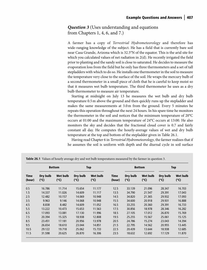
Example Questions and Answers 407
Question 3 (Uses understanding and equations from Chapters 1, 4, 6, and 7.)
A farmer has a copy of Terrestrial Hydrometeorology and therefore has
wide-ranging knowledge of the subject. He has a field that is currently bare soil
near Casa Grande, Arizona which is 32.5°N of the equator. This is the arid site for
which you calculated values of net radiation in 2(d). He recently irrigated the field
prior to planting and the sandy soil is close to saturated. He decides to measure the
evaporation loss from the field but he only has three thermometers and a set of tall
stepladders with which to do so. He installs one thermometer in the soil to measure
the temperature very close to the surface of the soil. He wraps the mercury bulb of
a second thermometer in a small piece of cloth that he is careful to keep moist so
that it measures wet bulb temperature. The third thermometer he uses as a dry
bulb thermometer to measure air temperature.
Starting at midnight on July 13 he measures the wet bulb and dry bulb
temperature 0.5 m above the ground and then quickly runs up the stepladder and
makes the same measurements at 3.0 m from the ground. Every 5 minutes he
repeats this operation throughout the next 24 hours. In his spare time he monitors
the thermometer in the soil and notices that the minimum temperature of 20°C
occurs at 01:00 and the maximum temperature of 24°C occurs at 13:00. He also
monitors the sky and decides that the fractional cloud cover is 0.7 and fairly
constant all day. He computes the hourly-average values of wet and dry bulb
temperature at the top and bottom of the stepladder given in Table 26.1.
Having read Chapter 6 in Terrestrial Hydrometeorology, the farmer realizes that if
he assumes the soil is uniform with depth and the diurnal cycle in soil surface
Table 26.1 Values of hourly average dry and wet bulb temperatures measured by the farmer in question 3.
Bottom Top Bottom Top
Time (hour)
Dry bulb (°C)
Wet bulb (°C)
Dry bulb (°C)
Wet bulb (°C)
Time (hour)
Dry bulb (°C)
Wet bulb (°C)
Dry bulb (°C)
Wet bulb (°C)
0.5 16.786 11.714 15.654 11.177 12.5 33.139 21.096 28.347 16.7031.5 14.337 11.026 14.609 11.117 13.5 34.790 21.547 29.391 17.0432.5 12.482 10.157 14.069 10.948 14.5 34.820 21.365 29.932 17.0933.5 9.963 9.146 14.068 10.948 15.5 34.600 20.918 29.931 16.8884.5 8.838 8.482 14.609 11.052 16.5 33.255 20.360 29.391 16.7335.5 13.222 10.473 15.653 11.563 17.5 30.856 18.978 28.346 16.2826.5 17.093 13.081 17.130 11.996 18.5 27.105 17.012 26.870 15.7697.5 20.394 15.325 18.938 12.808 19.5 25.255 15.567 25.061 15.1258.5 23.451 17.181 20.956 13.978 20.5 24.786 15.274 23.043 14.3949.5 26.654 18.610 23.044 14.851 21.5 22.795 14.562 20.955 13.44510.5 29.122 19.718 25.062 15.733 22.5 20.439 13.644 18.938 12.68511.5 31.598 20.625 26.870 16.306 23.5 18.632 12.692 17.129 11.870
Shuttleworth_c26.indd 407Shuttleworth_c26.indd 407 11/3/2011 6:37:23 PM11/3/2011 6:37:23 PM
408 Example Questions and Answers
temperature is sinusoidal, and if he chooses the form of the sinusoidal wave to agree
with the timing and magnitude of the minimum and maximum soil temperatures
that he measured and also selects values of soil properties appropriate for the moist
sandy soil, he can calculate the soil heat flux at any time during the day.
(a) What were the values of the mean soil surface temperature, and the
amplitude and the time slip of the cycle in soil surface temperature that he
selected?
(b) What were the values of soil thermal conductivity, ks, and thermal
diffusivity, αs, that he selected, what was the value of damping depth, D, for
the daily time period (expressed in seconds) that he calculated. Which
equation from Terrestrial Hydrometeorology did he use to calculate the
instantaneous surface soil heat flux?
The farmer assumes that the psychrometric constant is 0.0667 kPa K−1 when
applying the wet-bulb equation and when calculating the Bowen ratio. For
simplicity he also assumes that the difference in virtual potential temperature is
equal to the difference in measured air temperature between the two levels. (This
is a common assumption when calculating Bowen ratio). In the course of his
calculations he found that the all-day average air temperature and vapor pressure
at the bottom level were the same as those you calculated and used in question
2(a). Using these values with the day of the year and latitude of the site he was able
to calculate the same estimates of net radiation for this arid site that you calculated
in question 2(d). You can therefore adopt those values of hourly net radiation for
use in this question.
(c) Develop a spreadsheet to tabulate the values of vapor pressure at the bot-
tom level, vapor pressure at the top level, Bowen ratio, net radiation [copied
from 2(e)], soil heat flux, available energy, latent heat flux and sensible heat
flux at hourly intervals between 0.5 and 23.5 hours.
(d) Plot the calculated net radiation, soil heat flux, available energy, latent heat
flux and sensible heat flux as a function of time through the day.
(e) What were the all-day average values of the Bowen ratio and Evaporative
Fraction at his site on this day?
(f) Suppose the farmer had chosen to neglect soil heat flux in his calculation of
available energy. Without recalculating all the rates, can you suggest
whether he would have overestimated or underestimated the all-day
average evaporative fraction and explain why?
Question 4 (Uses understanding from Chapters 1, 2, and 8.)
(a) Shuttleworth says, ‘As an annual-average, the value is about 1.2 m. However
we, as land dwellers, see only about 10% of this, and we lose almost two-
thirds back to the atmosphere. We keep an even smaller proportion
Shuttleworth_c26.indd 408Shuttleworth_c26.indd 408 11/3/2011 6:37:23 PM11/3/2011 6:37:23 PM
Example Questions and Answers 409
in Arizona.’ In your opinion, what is Shuttleworth talking about? The
annual-average of what is about 1.2 m? How do we lose two-thirds back to
the atmosphere? Approximately what proportion do we keep in Arizona?
(b) Shuttleworth says, ‘These two components of these models have jargon
names and are run alternately. The first applies the conservation laws while
the second, by representing relevant processes, changes the divergence
terms in these laws prior to their next application.’ In your opinion, what
components of what models is he talking about and what are their jargon
names. Which ‘laws’ does he refer to? Can you suggest some of the relevant
processes that change the divergence terms in these laws?
(c) Shuttleworth says, ‘Of course, if all the continents were constrained to be in
the tropics then, as a global average, the proportion of the Sun’s radiant
energy reflected at the Earth’s surface would vary less between summer and
winter.’ In your opinion, what is at least one reason why Shuttleworth might
be correct?
(d) Shuttleworth says, ‘Most of the time the temperature gradient in the lower
atmosphere is less than the dry adiabatic lapse rate. Water vapor is also
strongly concentrated at the bottom of the atmosphere. Presumably, the
same processes are responsible for both of these phenomena.’ In your
opinion, could Shuttleworth’s presumption be correct? What process or
processes might simultaneously reduce the actual lapse rate below the
adiabatic rate and also reduce the vapor content of the atmosphere at levels
well above the ground?
(e) Shuttleworth says, ‘These models are used in three main ways, each with a
different objective. However, in fact, one application was a by-product of
the original model application. “Initiation” is a keyword in all of these
applications.’ In your opinion, now what is Shuttleworth talking about?
What models? What are the three different objectives? Can you suggest
why he puts emphasis on model initiation?
(f) Shuttleworth says, ‘The specific heat is 4 times bigger and the density is
nearly 1000 times bigger. If this wasn’t true, we might have http://www.
weather.gov/ but we probably would not have http://www.cpc.ncep.noaa.
gov/’ In your opinion, what has a specific heat and density respectively 4
and 1000 times bigger than what? If this were not the case, can you explain
why in your opinion this might mean that http://www.cpc.ncep.noaa.gov/
would not be needed but http://www.weather.gov/ likely still would be?
(g) Shuttleworth says, ‘One important potential consequence of ‘greenhouse
warming’ is that it will enhance the hydrological cycle. It is interesting that
non-linearity in the basic relationship that would cause this enhancement
tends to compensate for the projected warming being twice as large at the
poles than at the equator.’ In your opinion, what does Shuttleworth mean
by this? Can you suggest what basic relationship might allow greenhouse
warming to enhance the hydrological cycle? Why might this relationship
be more effective at the equator, thus compensating for the potentially
enhanced warming at the poles?
Shuttleworth_c26.indd 409Shuttleworth_c26.indd 409 11/3/2011 6:37:23 PM11/3/2011 6:37:23 PM

410 Example Questions and Answers
Question 5 (Uses understanding from Chapter 9.)
The planet Malleable is fascinating. In many respects it is identical to the Earth. It
has identical dimensions and is located in a solar system identical to ours. It rotates
around an identical sun, in an identical orbit, and its solar declination changes
seasonally as does the Earth’s. Moreover, on average, the relative area of oceans and
continents is the same as that on Earth. The planet is the adopted home to an
advanced civilization that can manipulate the location of the continents on
Malleable’s surface. When it was settled, the ‘Founding Fathers’ of Malleable chose
to distribute these continents as shown in Fig. 26.1.
The planet Malleable is governed by a single planetary government. It is election
year and three main parties are seeking election. They are as follows.
The Reduce Warm Deserts (RWD) Party, whose platform is to redefine the
continents so as to reduce the non-productive continental areas that are deserts
on planet Malleable.
The Reduce Tropical Storms (RTS) Party, whose platform is to redefine the conti-
nents so as to reduce the ‘seed areas’ for tropical storms on planet Malleable.
The Maximize Monsoons (MM) Party, the central theme of whose platform is to
enhance seasonal precipitation in subtropical regions and thus allow the
production of additional seasonal crops on planet Malleable.
Each political party has devised a banner that expresses their ideas symbolically by
approximately representing the new continental distributions they are respectively
suggesting. As the most effective printer on Malleable, you have been awarded the
Current continental arrangement
Banner A
Banner B
Banner C
Figure 26.1 Current
continental arrangement on
planet Malleable and the three
banners used by three political
parties in the election.
Shuttleworth_c26.indd 410Shuttleworth_c26.indd 410 11/3/2011 6:37:23 PM11/3/2011 6:37:23 PM
Example Questions and Answers 411
contract to print these banners. Unfortunately the three party symbols have
arrived at your printing works without you knowing which symbol belongs to
which party. On the basis of your understanding derived from Terrestrial
Hydrometeorology, you must choose the most appropriate symbol for each party’s
banner. These symbols are also shown in Fig. 26.1.
(a) In your opinion, which banner (A, B, or C) most likely represents the
continental distribution advocated by the RWD Party and briefly explain
what you think is the basis for them suggesting this particular continental
distribution.
(b) In your opinion, which banner (A, B, or C) most likely represents the
continental distribution advocated by the RTS Party and briefly explain
what you think is the basis for them suggesting this particular continental
distribution.
(c) In your opinion, which banner (A, B, or C) most likely represents the
continental distribution advocated by the MM Party and briefly explain
what you think is the basis for them suggesting this particular continental
distribution.
Late in the election campaign, a fourth party, the Reduce El Niño (REN) Party,
emerges. Their objective is to seek to reduce the severity of fluctuations in climate
associated with building unstable ‘warm pools’ in Malleable’s tropical oceans.
Their hope is to gain a share of power by forming a coalition with one of the other
parties after the election. They see most opportunity of making a deal with either
the RWD or the RTS parties and have opened secret discussions with these two
parties before the election.
(d) In your opinion, how might the RWD Party be arguing for the support of
the REN Party after the election?
(e) In your opinion, how might the RTS Party be arguing for the support of the
REN Party after the election?
Question 6 (Uses understanding from Chapters 9, 10 and 11.)
Briefly answer the following.
(a) In your opinion, what is the fundamental cause of the difference between
the thermal structure of the oceans and the atmosphere? What is your
opinion on the consequence of the above phenomenon on the vertical
structure of the oceans, and say how this changes with latitude and
season.
(b) A student said, ‘Ocean currents tend to go north on the eastern sides of
continents, and south on the western side of continents’. In your opinion, is
the student correct? Why?
Shuttleworth_c26.indd 411Shuttleworth_c26.indd 411 11/3/2011 6:37:23 PM11/3/2011 6:37:23 PM
412 Example Questions and Answers
(c) In your opinion, why do ocean currents tend to behave this way?
(d) Discuss the statement, ‘The geographical distribution of land masses
influences the effect of ocean circulation on tropical Sea Surface
Temperature’ in the context of the Atlantic Ocean, and give your opinion
on any consequences on the relative frequency of tropical storms in Cuba
and in northeast Brazil.
(e) A student said, ‘The hydroclimatic mechanism which most influences the
food supply of half the world’s population is related to difference in the way
surface radiation is shared for continents and oceans.’ In your opinion,
what did she mean?
(f) For clouds to occur in the atmosphere a mechanism which gives rising air
and therefore cooling air is required. In your opinion, what are two other
requirements and which of them is most likely to be the limiting
requirement?
(g) If a parcel of air is moister than its surroundings but it has the same
temperature and pressure, in your opinion will it tend to rise or will it tend
to fall? Briefly explain why.
(h) In convective conditions parcels of air are heated and start to rise because
they are warmer and lighter. As soon as a parcel rises the air cools. In your
opinion why does this cooling not necessarily stop the air parcel rising to
the cloud condensation level?
(i) Once the cloud condensation level is reached, cloud formation begins. Give
your opinion on what effect the condensation process will have on the
buoyancy of the parcel of air and its further ascent in the cloud.
(j) In a particular mid-latitude cloud, the air temperature is -25°C. In your
opinion, which phases of water (solid, liquid or vapor) are likely to be
present in the cloud, and what is likely to be the most important physical
mechanism giving ice particle growth in the cloud.
Question 7 (Uses understanding from Chapters 12, 13 and 14.)
(a) Draw a diagram of what in your opinion is the ideal site and mounting for
a rain gauge. It should show its relation to surrounding objects and to the
ground. Give a brief explanation of why you consider your design to be
good. Discuss this design with your instructor.
(b) Obtain values of mean monthly precipitation for a site that interests you
(e.g., your home town, state, or country). Compute the Seasonality Index
from these data using the formulae given in your class notes (or an
alternative measure of seasonality if you prefer; there are alternative
measures.) Comment on what this index implies about the seasonality of
the precipitation climate that you choose.
(c) Using the same data you used in question 7(b), draw a ‘pie’ diagram to
illustrate the seasonal behavior of the rainfall showing the percentage
contributions to the annual rainfall in each month.
Shuttleworth_c26.indd 412Shuttleworth_c26.indd 412 11/3/2011 6:37:24 PM11/3/2011 6:37:24 PM
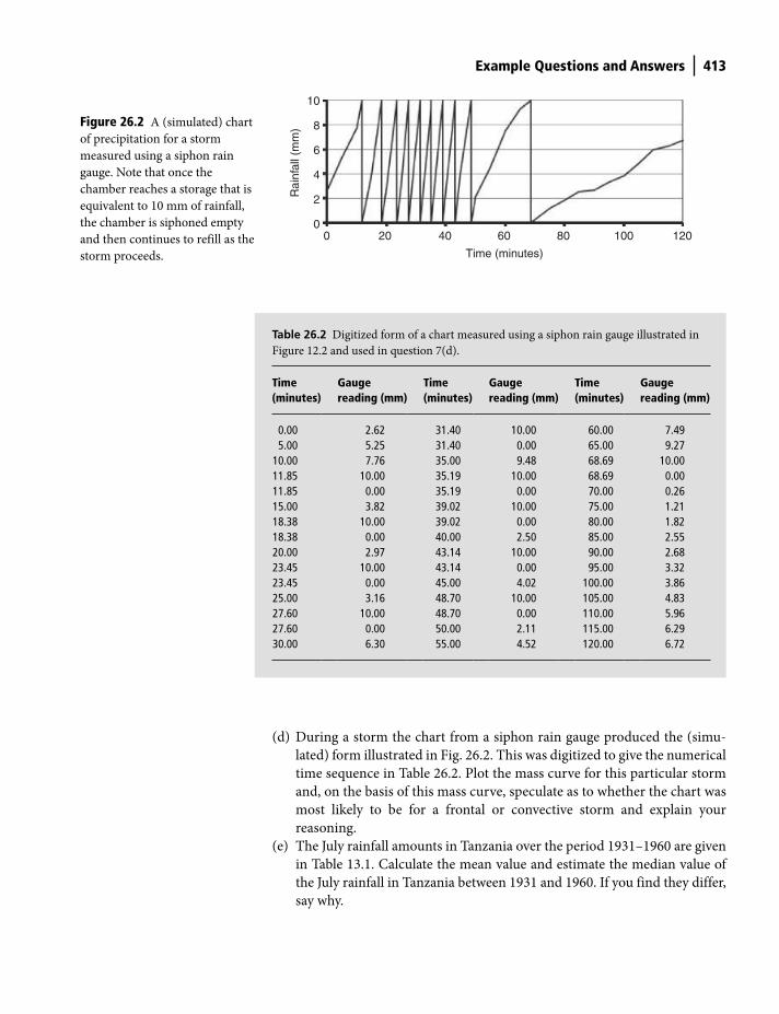
Example Questions and Answers 413
(d) During a storm the chart from a siphon rain gauge produced the (simu-
lated) form illustrated in Fig. 26.2. This was digitized to give the numerical
time sequence in Table 26.2. Plot the mass curve for this particular storm
and, on the basis of this mass curve, speculate as to whether the chart was
most likely to be for a frontal or convective storm and explain your
reasoning.
(e) The July rainfall amounts in Tanzania over the period 1931–1960 are given
in Table 13.1. Calculate the mean value and estimate the median value of
the July rainfall in Tanzania between 1931 and 1960. If you find they differ,
say why.
10
8
6
4
2
00 20 40 60
Time (minutes)
80 100 120
Rai
nfal
l (m
m)Figure 26.2 A (simulated) chart
of precipitation for a storm
measured using a siphon rain
gauge. Note that once the
chamber reaches a storage that is
equivalent to 10 mm of rainfall,
the chamber is siphoned empty
and then continues to refill as the
storm proceeds.
Table 26.2 Digitized form of a chart measured using a siphon rain gauge illustrated in
Figure 12.2 and used in question 7(d).
Time (minutes)
Gauge reading (mm)
Time (minutes)
Gauge reading (mm)
Time (minutes)
Gauge reading (mm)
0.00 2.62 31.40 10.00 60.00 7.495.00 5.25 31.40 0.00 65.00 9.27
10.00 7.76 35.00 9.48 68.69 10.0011.85 10.00 35.19 10.00 68.69 0.0011.85 0.00 35.19 0.00 70.00 0.2615.00 3.82 39.02 10.00 75.00 1.2118.38 10.00 39.02 0.00 80.00 1.8218.38 0.00 40.00 2.50 85.00 2.5520.00 2.97 43.14 10.00 90.00 2.6823.45 10.00 43.14 0.00 95.00 3.3223.45 0.00 45.00 4.02 100.00 3.8625.00 3.16 48.70 10.00 105.00 4.8327.60 10.00 48.70 0.00 110.00 5.9627.60 0.00 50.00 2.11 115.00 6.2930.00 6.30 55.00 4.52 120.00 6.72
Shuttleworth_c26.indd 413Shuttleworth_c26.indd 413 11/3/2011 6:37:24 PM11/3/2011 6:37:24 PM
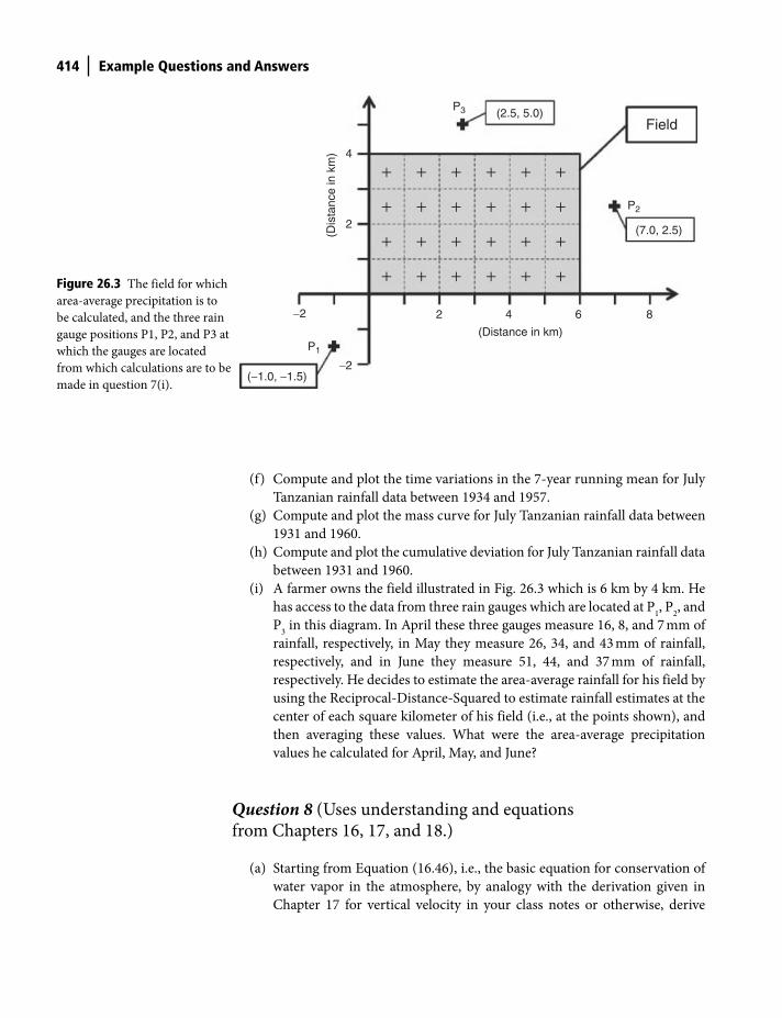
414 Example Questions and Answers
(f) Compute and plot the time variations in the 7-year running mean for July
Tanzanian rainfall data between 1934 and 1957.
(g) Compute and plot the mass curve for July Tanzanian rainfall data between
1931 and 1960.
(h) Compute and plot the cumulative deviation for July Tanzanian rainfall data
between 1931 and 1960.
(i) A farmer owns the field illustrated in Fig. 26.3 which is 6 km by 4 km. He
has access to the data from three rain gauges which are located at P1, P
2, and
P3 in this diagram. In April these three gauges measure 16, 8, and 7 mm of
rainfall, respectively, in May they measure 26, 34, and 43 mm of rainfall,
respectively, and in June they measure 51, 44, and 37 mm of rainfall,
respectively. He decides to estimate the area-average rainfall for his field by
using the Reciprocal-Distance-Squared to estimate rainfall estimates at the
center of each square kilometer of his field (i.e., at the points shown), and
then averaging these values. What were the area-average precipitation
values he calculated for April, May, and June?
Question 8 (Uses understanding and equations from Chapters 16, 17, and 18.)
(a) Starting from Equation (16.46), i.e., the basic equation for conservation of
water vapor in the atmosphere, by analogy with the derivation given in
Chapter 17 for vertical velocity in your class notes or otherwise, derive
2−2
−2
4
4
(Distance in km)
6 8
2
P1
P2
P3
(−1.0, −1.5)
(2.5, 5.0)
(7.0, 2.5)
Field
+
+
+
+
+
+
+
+
+
+
+
+
+
+
+
+
+
+
+
+
+
+
+
+
(Dis
tanc
e in
km
)
Figure 26.3 The field for which
area-average precipitation is to
be calculated, and the three rain
gauge positions P1, P2, and P3 at
which the gauges are located
from which calculations are to be
made in question 7(i).
Shuttleworth_c26.indd 414Shuttleworth_c26.indd 414 11/3/2011 6:37:25 PM11/3/2011 6:37:25 PM
Example Questions and Answers 415
Equation (26.3), the prognostic equation describing for water vapor
fluctuations in the atmosphere:
( ) ( ) ( )
2
' ' ' ' ' '
a a
Sq q q q Eu v w qt x y z
u q v q w qx y z
∂ ∂ ∂ ∂+ + + = + + ∇
∂ ∂ ∂ ∂⎛ ⎞∂ ∂ ∂
− + +⎜ ⎟∂ ∂ ∂⎝ ⎠
ur r
(26.3)
explaining each step in the derivation as you do so.
The prognostic equations describing the conservation of mean potential tem-
perature has a similar form, thus:
( ) ( ) ( )
2
' ' ' ' ' '
n
a p a p
R Eu v wt x y z c c
u v wx y z
θ
∇∂θ ∂θ ∂θ ∂θ+ + + = − − + υ ∇ θ
∂ ∂ ∂ ∂⎛ ⎞∂ θ ∂ θ ∂ θ
− + +⎜ ⎟∂ ∂ ∂⎝ ⎠
r r
(26.4)
Give the terms that become negligible in Equations (26.3) and (26.4) when the
following assumptions are made.
(b) There is no mechanism for creating water vapor chemically in the
atmosphere.
(c) There is no phase change between water vapor and liquid/solid water.
(d) There is no horizontal or vertical change in the net radiation flux in the
ABL.
(e) Molecular diffusion can be neglected.
(f) There is no ascent or subsidence (i.e. no persistent rising or sinking of the
air).
(g) There is no horizontal divergence of turbulent fluxes.
(h) There is no horizontal advection of humidity or potential temperature.
(i) After making all of the above simplifying assumptions, write down the
(much simpler) versions of Equations (26.3) and (26.4) which then apply.
Figure 26.4 sketches the simplified average height dependence of the sensible heat
flux H(z) and the moisture flux E(z) through the daytime atmospheric boundary
layer over uniform terrain in cloudless conditions when there is no subsidence. It
labels five levels different levels (i), (ii), (iii), (iv), and (v). You are only allowed to
choose between the following three options for changes in air temperature – be
warmer, be cooler, or change little; and you are only allowed to choose between the
following three options for changes in atmospheric humidity – be wetter, be drier,
or change little. On the basis of the answer to question (i), say how the temperature
and humidity will change over the next few minutes at the levels given below.
Shuttleworth_c26.indd 415Shuttleworth_c26.indd 415 11/3/2011 6:37:25 PM11/3/2011 6:37:25 PM
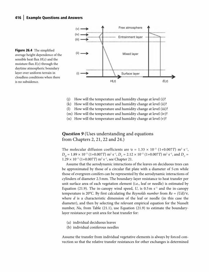
416 Example Questions and Answers
(j) How will the temperature and humidity change at level (i)?
(k) How will the temperature and humidity change at level (ii)?
(l) How will the temperature and humidity change at level (iii)?
(m) How will the temperature and humidity change at level (iv)?
(n) How will the temperature and humidity change at level (v)?
Question 9 (Uses understanding and equations from Chapters 2, 21, 22 and 24.)
The molecular diffusion coefficients are υ = 1.33 × 10⁻⁵ (1+0.007T) m2 s−1,
DH = 1.89 × 10⁻⁵ (1+0.007T) m2 s−1, D
V = 2.12 × 10⁻⁵ (1+0.007T) m2 s−1, and D
C =
1.29 × 10⁻⁵ (1+0.007T) m2 s−1, see Chapter 21.
Assume that the aerodynamic interactions of the leaves on deciduous trees can
be approximated by those of a circular flat plate with a diameter of 5 cm while
those of evergreen conifers can be represented by the aerodynamic interactions of
cylinders of diameter 2.5 mm. The boundary-layer resistance to heat transfer per
unit surface area of each vegetation element (i.e., leaf or needle) is estimated by
Equation (21.9). The in-canopy wind speed, U, is 0.5 m s−1 and the in-canopy
temperature is 20°C. By first calculating the Reynolds number from Re = (Ud)/n,
where d is a characteristic dimension of the leaf or needle (in this case the
diameter), and then by selecting the relevant empirical equation for the Nusselt
number, Nu, from Table (21.1), use Equation (21.9) to estimate the boundary-
layer resistance per unit area for heat transfer for:
(a) individual deciduous leaves
(b) individual coniferous needles
Assume the transfer from individual vegetative elements is always by forced con-
vection so that the relative transfer resistances for other exchanges is determined
Mixed layer
Surface layer
Entrainment layer
Free atmosphere(v)
(iv)
(iii)
(ii)
(i)
H(z) E(z)
Figure 26.4 The simplified
average height dependence of the
sensible heat flux H(z) and the
moisture flux E(z) through the
daytime atmospheric boundary
layer over uniform terrain in
cloudless conditions when there
is no subsidence.
Shuttleworth_c26.indd 416Shuttleworth_c26.indd 416 11/3/2011 6:37:27 PM11/3/2011 6:37:27 PM
Example Questions and Answers 417
only by their relative diffusion coefficients, see Equations (21.10) and (21.11).
From the answer to Question 9(b), estimate the boundary-layer resistance for:
(c) vapor transfer for coniferous needles;
(d) carbon dioxide transfer for coniferous needles.
(e) Equations (22.2), (22.3) and (22.4), approximately describe how the zero
plane displacement, d, and aerodynamic roughness length, zo, of a vegeta-
tion stand vary relative to the crop height, h, as a function of the leaf area
index, LAI, for a canopy with maximum vegetation density approximately
halfway through canopy depth. Assuming the aerodynamic roughness
length for bare soil, z0’, can be neglected, plot the values of (d/h) and (z
o/h)
as a function of leaf area index in the range LAI = 0 to 5 and comment on
why these two ratios vary with LAI in this way. Calculate the values of (d/h)
and (zo/h) when LAI = 4 for use in 9(f).
(f) Assume the aerodynamic resistance for latent and sensible heat transfer
to a vegetation stand in neutral conditions, ra, is given by Equation (22.9).
If both wind speed and vapor pressure deficit are measured 2 m above
the top of a 10 cm high grass stand, at 2 m above the top of a 1 m high
cereal crop stand, and at 2 m above the top of a 30 m high forest stand,
and all these stands have LAI = 4, plot the aerodynamic resistance of
these three vegetation stands as a function of wind speed from 0.25 m s−1
to 8 m s−1.
(g) Some SVAT represent the behavior of the surface resistance using the
Jarvis-Stewart model. Assume the surface conductance for the forest stand
considered in (f) is given by Equation (24.1) with g0 = 40 mm s−1 and g
M = 1
(i.e., there is no soil moisture stress); and with gR, g
D , and g
T , given
by Equations (24.2), (24.3) and (24.4), and (24.5), with KR = 200 W m−2,
KD
1 = –0.307 kPa−1, KD
2 = 0.019 kPa−2, TL =273 K, T
0 = 293 K, and T
H = 313 K.
Plot the variation in the individual stress functions gR, g
D , and g
T over the
solar radiation ranges 0–1000 Wm−2, VPD range 0–4 kPa, and temperature
range 0–40°C, respectively. If any stress function is calculated to be less
than zero, it should be set to zero. (Hint: do your calculations look plausible
in comparison with Fig. 24.5?)
In the following, assume the meteorological data given in Table 26.3 were measured
2 m above the top of the 30 m high forest and that it is acceptable to use the
aerodynamic resistance ra calculated in 9(f) and the formulae for surface
conductance specified in 9(g) to calculate the surface resistance rs (= g
s−1).
(h) Plot the variation through the day of the individual stress functions gR, g
D ,
and gT , and also the total stress function, i.e., the product (g
R g
D g
T g
M).
(i) Using the Penman-Monteith equation (Equation 21.33) and the surface
energy balance, plot the variation through the day of available energy,
latent heat and sensible heat fluxes.
Shuttleworth_c26.indd 417Shuttleworth_c26.indd 417 11/3/2011 6:37:28 PM11/3/2011 6:37:28 PM
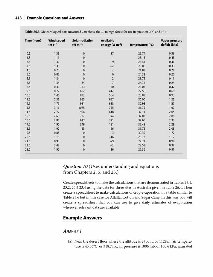
418 Example Questions and Answers
Table 26.3 Meteorological data measured 2 m above the 30 m high forest for use in question 9(h) and 9(i).
Time (hour) Wind speed (m s−1)
Solar radiation (W m−2)
Available energy (W m−2) Temperature (°C)
Vapor pressure deficit (kPa)
0.5 1.39 0 17 26.74 0.561.5 1.11 0 1 26.13 0.482.5 1.30 0 9 25.47 0.413.5 1.36 0 −2 25.08 0.334.5 0.70 0 2 24.83 0.285.5 0.87 0 0 24.32 0.206.5 1.84 0 2 23.72 0.117.5 1.34 84 7 24.74 0.248.5 0.36 333 30 26.02 0.429.5 0.77 602 412 27.56 0.69
10.5 1.46 832 564 28.89 0.9311.5 2.36 965 697 30.00 1.2512.5 1.75 981 638 30.93 1.5713.5 3.16 1075 755 31.75 1.9714.5 2.77 994 618 32.11 2.0515.5 2.68 732 374 32.03 2.0916.5 2.85 617 321 32.66 2.3317.5 1.90 346 131 32.48 2.2918.5 1.97 85 26 31.75 2.0819.5 0.88 0 −3 30.39 1.7220.5 1.18 0 −16 28.72 1.1221.5 0.98 0 −9 27.71 0.9022.5 2.42 0 −2 27.58 0.9223.5 1.90 0 16 27.36 0.91
Question 10 (Uses understanding and equations from Chapters 2, 5, and 23.)
Create spreadsheets to make the calculations that are demonstrated in Tables 23.1,
23.2, 23.3 23.4 using the data for three sites in Australia given in Table 26.4. Then
create a spreadsheet to make calculations of crop evaporation in a table similar to
Table 23.6 but in this case for Alfalfa, Cotton and Sugar Cane. In this way you will
create a spreadsheet that you can use to give daily estimates of evaporation
wherever relevant data are available.
Example Answers
Answer 1
(a) Near the desert floor where the altitude is 3700 ft, or 1128 m, air tempera-
ture is 45.56°C, or 318.71 K, air pressure is 1006 mb, or 100.6 kPa, saturated
Shuttleworth_c26.indd 418Shuttleworth_c26.indd 418 11/3/2011 6:37:28 PM11/3/2011 6:37:28 PM
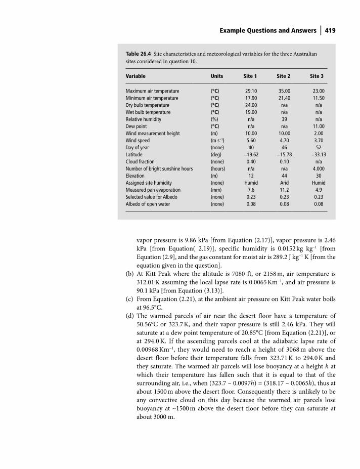
Example Questions and Answers 419
vapor pressure is 9.86 kPa [from Equation (2.17)], vapor pressure is 2.46
kPa [from Equation( 2.19)], specific humidity is 0.0152 kg kg−1 [from
Equation (2.9], and the gas constant for moist air is 289.2 J kg−1 K [from the
equation given in the question].
(b) At Kitt Peak where the altitude is 7080 ft, or 2158 m, air temperature is
312.01 K assuming the local lapse rate is 0.0065 Km−1, and air pressure is
90.1 kPa [from Equation (3.13)].
(c) From Equation (2.21), at the ambient air pressure on Kitt Peak water boils
at 96.5°C.
(d) The warmed parcels of air near the desert floor have a temperature of
50.56°C or 323.7 K, and their vapor pressure is still 2.46 kPa. They will
saturate at a dew point temperature of 20.85°C [from Equation (2.21)], or
at 294.0 K. If the ascending parcels cool at the adiabatic lapse rate of
0.00968 Km−1, they would need to reach a height of 3068 m above the
desert floor before their temperature falls from 323.71 K to 294.0 K and
they saturate. The warmed air parcels will lose buoyancy at a height h at
which their temperature has fallen such that it is equal to that of the
surrounding air, i.e., when (323.7 – 0.0097h) = (318.17 – 0.0065h), thus at
about 1500 m above the desert floor. Consequently there is unlikely to be
any convective cloud on this day because the warmed air parcels lose
buoyancy at ∼1500 m above the desert floor before they can saturate at
about 3000 m.
Table 26.4 Site characteristics and meteorological variables for the three Australian
sites considered in question 10.
Variable Units Site 1 Site 2 Site 3
Maximum air temperature (°C) 29.10 35.00 23.00Minimum air temperature (°C) 17.90 21.40 11.50Dry bulb temperature (°C) 24.00 n/a n/aWet bulb temperature (°C) 19.00 n/a n/aRelative humidity (%) n/a 39 n/aDew point (°C) n/a n/a 11.00Wind measurement height (m) 10.00 10.00 2.00Wind speed (m s−1) 5.60 4.70 3.70Day of year (none) 40 46 52Latitude (deg) −19.62 −15.78 −33.13Cloud fraction (none) 0.40 0.10 n/aNumber of bright sunshine hours (hours) n/a n/a 4.000Elevation (m) 12 44 30Assigned site humidity (none) Humid Arid HumidMeasured pan evaporation (mm) 7.6 11.2 4.9Selected value for Albedo (none) 0.23 0.23 0.23Albedo of open water (none) 0.08 0.08 0.08
Shuttleworth_c26.indd 419Shuttleworth_c26.indd 419 11/3/2011 6:37:29 PM11/3/2011 6:37:29 PM
420 Example Questions and Answers
Answer 2
(a) At this site on this day, the all-day average air temperature is 22°C, or
295.13 K, the saturated vapor pressure is 2.644 kPa, and the vapor pressure
is 1.322 kPa.
(b) When calculating net longwave radiation, the effective emissivity e’ = 0.194
[from Equation (5.23)] and assuming c = 0.7 all through the day, for an arid
site the empirical cloud factor f = 0.37 [from Equation (5..25)]. The esti-
mated all-day average net longwave radiation is therefore –28 W m−2 [from
Equation (5..22)].
(c) Were this a humid site the empirical cloud factor, f, would then be 0.533
[from Equation (5..24)] and the estimated all-day average net longwave
radiation would be -41 W m−2 [from Equation (5..22)].
(d) July 12 is Day Of Year 193, hence the eccentricity factor dl = 0.968 [from
Equation (5.5)] and the solar declination δ = 0.385 radians [from Equation
(5.8)]. The latitude of the site is 32.5°N, which is +0.567 radians, and the
hour angle, w, can be calculated in radians from the time of day, t, in hours
[using Equation (5.10)], with t running in hourly increments from 0.5 to
23.5. Consequently, the solar radiation at the top of the atmosphere, Stop, can
be calculated [from Equation (26.1)] and solar radiation at the ground, Sgrnd,
calculated [from Equation (26.2)]. Values of net solar radiation can then
be calculated for each value of t by allowing for the albedo of 0.23 [by
comparison with Equation (5.18)]. Values of net radiation can then be cal-
culated for each value of t by adding the relevant values of longwave radiation
for arid and humid conditions calculated in sections (b) and (c), respectively.
The resulting values of solar radiation, net solar radiation, and net radiation
for an arid and a humid site are given in Table 26.5 and plotted in Fig. 26.5.
(e) The required all-day average values are 190 W m−2 for (incoming) solar
radiation, 146 W m−2 for net solar radiation, 118 W m−2 for net radiation at
this arid site, and 105 W m−2 for net radiation were it assumed to be a
humid site.
(f) The required all-day average fluxes and plots of the diurnal variation in
solar, net solar, and net radiation for the Saskatoon site with fresh snow
cover on January 15 and grassland cover on July 15 are given in Fig. 26.6.
(g) The required all-day average fluxes and plots of the diurnal variation in
solar, net solar, and net radiation for the Manaus site on March 23 with for-
est and pastureland cover given in Fig. 26.7.
Answer 3
(a) The mean soil surface temperature, Tm
, is (24+20)/2 = 22°C, the amplitude
of the daily cycle, Ta, is (24–20)/2 = 2°C, and the time slip, t
o, which gives a
minimum 01.00 am and a maximum at 13.00 in Equation (6.11) is (7 ×
60 × 60) = 25,200 seconds.
Shuttleworth_c26.indd 420Shuttleworth_c26.indd 420 11/3/2011 6:37:29 PM11/3/2011 6:37:29 PM

Example Questions and Answers 421
(b) For saturated sandy soil the thermal conductivity, ks, is 2.20 W m−2 K−1 and
the thermal diffusivity, αs, is 0.74 × 10⁻⁶ m2 s−1. The damping depth, D, for
the daily time period P = (24 × 60 × 60) = 86,400 seconds is 0.143 m [from
Equation (6.13)]. The farmer used Equation (6.14) to estimate the instanta-
neous surface soil heat flux.
(c) The vapor pressure at the bottom level, vapor pressure at top level, Bowen
ratio, net radiation, soil heat flux, available energy, latent heat flux and sen-
sible heat flux are tabulated in Table 26.6.
(d) The net radiation, soil heat flux, available energy, latent heat flux and the sen-
sible heat flux are plotted as a function of time through the day in Fig. 26.8.
60 12Time (hrs)
18 24
Solar
Net (arid)Net (humid)
600
500
400
300
200
100
0
−100
Ene
rgy
flux
(W m
−2)
Figure 26.5 The diurnal cycle
of (incoming) solar radiation, net
solar radiation, longwave
radiation, and net radiation
calculated in 2(d) assuming it is
an arid and a humid site.
Table 26.5 Values of (incoming) solar radiation, net solar radiation, longwave radiation, and net radiation calculated in 2(d)
assuming it is both an arid and a humid site.
Hour (local)
Solar (W m−2)
Net solar (W m−2)
Net (arid) (W m−2)
Net (humid) (W m−2)
Hour (local)
Solar (W m−2)
Net solar (W m−2)
Net (arid) (W m−2)
Net (humid) (W m−2)
0.5 0 0 −28 −41 12.5 517 398 369 3571.5 0 0 −28 −41 13.5 489 376 348 3352.5 0 0 −28 −41 14.5 435 335 306 2943.5 0 0 −28 −41 15.5 358 276 248 2354.5 0 0 −28 −41 16.5 265 204 176 1635.5 53 41 12 0 17.5 161 124 95 836.5 161 124 95 83 18.5 53 41 12 07.5 265 204 176 163 19.5 0 0 −28 −418.5 358 276 248 235 20.5 0 0 −28 −419.5 435 335 306 294 21.5 0 0 −28 −41
10.5 489 376 348 335 22.5 0 0 −28 −4111.5 517 398 369 357 23.5 0 0 −28 −41
Shuttleworth_c26.indd 421Shuttleworth_c26.indd 421 11/3/2011 6:37:29 PM11/3/2011 6:37:29 PM
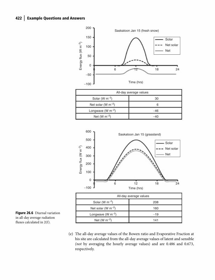
422 Example Questions and Answers
All-day average values
30
6
−46
−40
Solar (W m−2)
Net solar (W m−2)
Longwave (W m−2)
Net (W m−2)
All-day average values
208
160
−19
141
Solar (W m−2)
Net solar (W m−2)
Longwave (W m−2)
Net (W m−2)
200
150
100
50
0
−50
−100
0 6 12
Time (hrs)
18 24Ene
rgy
flux
(W m
−2)
Solar
Net solar
Net
Saskatoon Jan 15 (fresh snow)
−100
0
100
200
300
400
500
600
Time (hrs)
0 6 12 18 24
Solar
Net solar
Net
Saskatoon Jan 15 (grassland)
Ene
rgy
flux
(W m
−2)
Figure 26.6 Diurnal variation
in all-day average radiation
fluxes calculated in 2(f).
(e) The all-day average values of the Bowen ratio and Evaporative Fraction at
his site are calculated from the all-day average values of latent and sensible
(not by averaging the hourly average values) and are 0.486 and 0.673,
respectively.
Shuttleworth_c26.indd 422Shuttleworth_c26.indd 422 11/3/2011 6:37:30 PM11/3/2011 6:37:30 PM
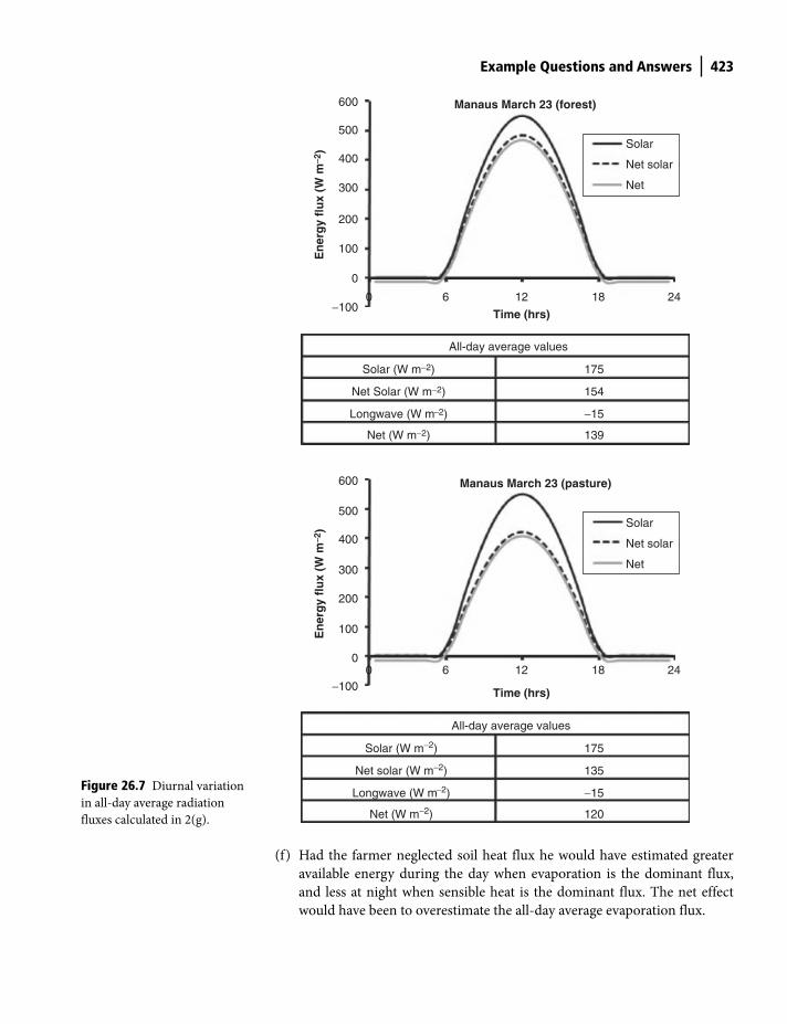
Example Questions and Answers 423
All-day average values
175
154
−15
139
Solar (W m−2)
Net Solar (W m−2)
Longwave (W m−2)
Net (W m−2)
All-day average values
175
135
−15
120
Solar (W m−2)
Net solar (W m−2)
Longwave (W m−2)
Net (W m−2)
600
500
400
300
200
0
100
−1000 6 12
Time (hrs)18 24
En
erg
y fl
ux
(W m
-2) Solar
Net solar
Net
Manaus March 23 (forest)
−100
0
100
200
300
400
500
600
Time (hrs)
0 6 12 18 24
Solar
Net solar
Net
Manaus March 23 (pasture)
En
erg
y fl
ux
(W m
-2)
Figure 26.7 Diurnal variation
in all-day average radiation
fluxes calculated in 2(g).
(f) Had the farmer neglected soil heat flux he would have estimated greater
available energy during the day when evaporation is the dominant flux,
and less at night when sensible heat is the dominant flux. The net effect
would have been to overestimate the all-day average evaporation flux.
Shuttleworth_c26.indd 423Shuttleworth_c26.indd 423 11/3/2011 6:37:31 PM11/3/2011 6:37:31 PM
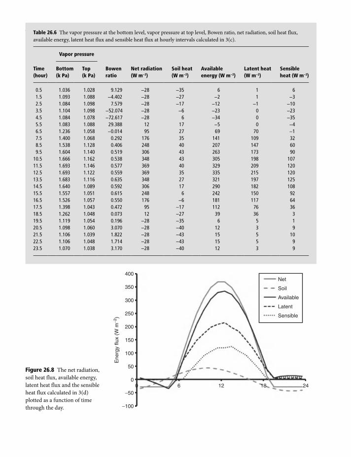
424 Example Questions and AnswersTable 26.6 The vapor pressure at the bottom level, vapor pressure at top level, Bowen ratio, net radiation, soil heat flux,
available energy, latent heat flux and sensible heat flux at hourly intervals calculated in 3(c).
Vapor pressure
Time (hour)
Bottom (k Pa)
Top (k Pa)
Bowen ratio
Net radiation (W m−2)
Soil heat (W m−2)
Available energy (W m−2)
Latent heat (W m−2)
Sensible heat (W m−2)
0.5 1.036 1.028 9.129 −28 −35 6 1 61.5 1.093 1.088 −4.402 −28 −27 −2 1 −32.5 1.084 1.098 7.579 −28 −17 −12 −1 −103.5 1.104 1.098 −52.074 −28 −6 −23 0 −234.5 1.084 1.078 −72.617 −28 6 −34 0 −355.5 1.083 1.088 29.388 12 17 −5 0 −46.5 1.236 1.058 −0.014 95 27 69 70 −17.5 1.400 1.068 0.292 176 35 141 109 328.5 1.538 1.128 0.406 248 40 207 147 609.5 1.604 1.140 0.519 306 43 263 173 90
10.5 1.666 1.162 0.538 348 43 305 198 10711.5 1.693 1.146 0.577 369 40 329 209 12012.5 1.693 1.122 0.559 369 35 335 215 12013.5 1.683 1.116 0.635 348 27 321 197 12514.5 1.640 1.089 0.592 306 17 290 182 10815.5 1.557 1.051 0.615 248 6 242 150 9216.5 1.526 1.057 0.550 176 −6 181 117 6417.5 1.398 1.043 0.472 95 −17 112 76 3618.5 1.262 1.048 0.073 12 −27 39 36 319.5 1.119 1.054 0.196 −28 −35 6 5 120.5 1.098 1.060 3.070 −28 −40 12 3 921.5 1.106 1.039 1.822 −28 −43 15 5 1022.5 1.106 1.048 1.714 −28 −43 15 5 923.5 1.070 1.038 3.170 −28 −40 12 3 9
400
350
300
250
200
150
100
50
0
−50
−100
0 6 12 18 24
Net
Soil
Available
Latent
Sensible
Ene
rgy
flux
(W m
−2)
Figure 26.8 The net radiation,
soil heat flux, available energy,
latent heat flux and the sensible
heat flux calculated in 3(d)
plotted as a function of time
through the day.
Shuttleworth_c26.indd 424Shuttleworth_c26.indd 424 11/3/2011 6:37:31 PM11/3/2011 6:37:31 PM

Example Questions and Answers 425
Answer 4
(a) Shuttleworth is speaking about the annual average evaporation from the
oceanic surfaces of the globe which is about 1.2 m per year. Around 90% of
this water falls back to the ocean while 10% moves and falls over land. When
averaged over all continental surfaces, about 65% of the precipitation falling
over land re-evaporates back to the atmosphere but in semi-arid areas the
proportion is higher. In Arizona, for instance, around 95% re-evaporates.
(b) Shuttleworth is talking about General Circulation models (GCMs). The
two components of these models he is referring to are the dynamics and the
physics. The dynamics applies conservation laws to calculate the fields of
atmospheric variables such as temperature, humidity and wind speed using
prescribed values for the divergence terms in these laws, see Chapters 16
and 17. The physics re-calculates the values of the divergence terms using
the (now modified) fields of atmospheric variables. Some of the processes
represented in the physics include radiation absorption, convection, and
precipitation processes in the atmosphere, and boundary layer and surface
exchange processes
(c) If all the Earth’s continents were clustered at the equator the seasonality of
the global average surface reflection coefficient for solar radiation, i.e. the
global average albedo, might well be less because, being on average warmer
than at present, they would presumably experience less snowfall. The
change in albedo associated with seasonal variations in snow and ice cover
is large because the albedo of fresh snow is around 80% while that for most
natural surfaces is around 20%. Alternative reasons for reduced seasonality
in global albedo include the possibility of reduced seasonal changes in the
vigor of the vegetation covering the continents.
(d) Shuttleworth is referring to the fact that the processes giving rise to
precipitation above, but comparatively close to the Earth’s surface, release
water vapor from the atmosphere and return it to the ground as precipitation,
which at the same time releases latent heat in the atmosphere. On average,
they therefore have the dual effect of reducing the lapse rate in the atmospheric
boundary layer so it is less than the adiabatic lapse rate while simultaneously
ensuring that atmospheric water vapor largely remains fairly near the surface.
(e) Presumably Shuttleworth is talking about GCMs again, because GCMs
have three main applications, namely (i) weather forecasting, (ii) climate
forecasting, and (iii) the synthesis of model-calculated fields of atmos-
pheric and surface variables across the entire globe as a by-product of
application (i). Weather forecasting seeks to predict actual weather a few
days ahead from well-defined initial conditions that may become the data
product (iii). In the case of (ii), initiation is less important because in this
application it is not actual weather but rather the statistics of weather (i.e.,
climate) that is the objective.
(f) Shuttleworth is respectively referring to the specific heat and density of
water relative to that of air. This difference means that the water in oceans
Shuttleworth_c26.indd 425Shuttleworth_c26.indd 425 11/3/2011 6:37:32 PM11/3/2011 6:37:32 PM
426 Example Questions and Answers
absorbs and releases energy more slowly than air and this is the fundamental
basis for the seasonal predictions that are the focus of interest of the Climate
Prediction Center whose website is at http://www.cpc.noaa.gov. Even if
seasonal predictions were not possible, presumably short-term prediction
would still be possible, and weather forecast centers such as the National
Weather Service at http://www.cpc.noaa.gov would still exist.
(g) ‘Greenhouse warming’ is predicted to increase near-surface air tempera-
tures. Since 70% of the Earth is covered with ocean, this likely will increase
surface evaporation rates because the saturated vapor pressure is a strong
function of temperature. Putting more water into the air as water vapor will
likely enhance the Earth’s overall hydrologic cycle by increasing the moisture
available for release by precipitation processes. At first sight, the effect will be
greatest at the poles because the projected temperature increases are greatest
there. However, saturated vapor pressure is a non-linear function of tem-
perature and the rate of change in saturated vapor pressure with temperature
is more than twice as large at 29°C (typical of sea surface temperature at the
equator) than it is at 0°C (typical of sea surface temperature at the poles).
Answer 5
The answers below give one opinion but, as is generally the case in politics,
different people have different opinions. If your opinions differ, discuss them with
your instructor.
(a) The RWD Party is probably using the banner C. Malleable has Hadley
Circulation similar to on Earth. Having looked through a telescope at their
sister planet, RWD Party followers notice that the resulting falling air
currents at approximately 30°N and 30°S of the equator suppress the
formation of precipitation and give rise to warm deserts when this occurs
over continents, e.g. the Sahara Desert. Their proposal is to remove the
continents at this band of latitudes.
(b) The RTS Party is probably using the banner A. The oceans on Malleable are
currently arranged to inhibit the inclusion of cold polar water in oceanic
circulation towards the equator. Looking through a telescope, followers of
the RTS Party notice that on their sister planet Earth, there is a marked
difference in the general shape of continental areas between the two
hemispheres. Those in Earth’s Northern Hemisphere are similar to those
on Malleable and inhibit inclusion of polar water in oceanic circulation.
However, the more open nature of the continents in the Earth’s Southern
Hemisphere allows cold polar water to penetrate towards the equator in the
western Pacific and Atlantic oceans. On average, this reduces the sea
surface temperature of equatorial western oceans in the Earth’s Southern
Hemisphere, and this in turn inhibits the production of tropical storms in
these regions. The RTS Party argues for opening the channels that link
Shuttleworth_c26.indd 426Shuttleworth_c26.indd 426 11/3/2011 6:37:32 PM11/3/2011 6:37:32 PM
Example Questions and Answers 427
polar and tropical oceans on Malleable so as to encourage the inclusion of
colder water towards their planet’s tropical oceans via oceanic circulation.
(c) The MM Party is probably using the banner B. Looking through a telescope,
followers of the MM Party notice that on their sister planet Earth there is
strong hydroclimatic feature that involves a marked seasonal reversal in
wind direction between areas on land and ocean. By listening in to the
radio broadcasts of weather services on Earth they learn this is called a
Monsoon. They notice that when the land surface is preferentially heated
by the shifting axis of rotation of the Sun there is a seasonal flow which
brings moisture over land that falls as precipitation in some months and
this is useful for growing agricultural crops. They also notice the effect is
greater when the flow is between a warm tropical ocean and large areas of
land that have a boundary which lies roughly parallel to the equator, e.g.,
the Indian Ocean and the continent of Asia. They are therefore suggesting
the continents on Malleable are arranged to favor such Monsoon flows.
(d) The RWD Party’s argument for the REN Party forming a coalition with
them is quite strong. They point out that relative to the existing continental
distribution, their proposed redistribution will significantly reduce the
portion of Malleable’s tropical ocean in which the Trade Winds can estab-
lish ‘warm pools’. The REN Party is negotiating for a bigger proportion of
the available land area at the equator but is facing opposition from the more
conservative faction of the RWD Party who have grown up in cooler cli-
mates with marked seasons.
(e) The RTS Party’s argument for the REN Party forming a coalition with them
is also reasonably convincing. They point out that their proposal will much
lessen the distance the Trade Winds have to establish ‘warm pools’ because of
the reduced distance between their four (as opposed to two) continents, and
because each proposed continent has more land area at the equator relative to
the existing continents. The REN party is negotiating for yet more continents
with more of their land area at the equator if they agree to form a coalition.
Answer 6
(a) Solar radiation heats the atmosphere from below, while it heats the oceans
from above. This results in a buoyant mixed layer on the surface of the
oceans which is typically 100–1000 m deep, and separated from the lower
ocean by the thermocline. The oceanic structure is fairly constant in time
in tropical regions, but the mixing layer changes depth with season at mid-
latitudes, being shallower and warmer in summer months when surface
heating is greater and the ensuing buoyancy of the surface water is greater.
(b) The student was a ‘Northo-centralist’ and was wrong. She should have said
‘ocean currents tend to go away from the equator on the eastern sides of
continents, and towards the equator on the western side of continents.’
(c) The near-surface mixed layer circulation of the oceans is primarily influ-
enced by the prevailing low level wind fields. The ocean, being massive, in
Shuttleworth_c26.indd 427Shuttleworth_c26.indd 427 11/3/2011 6:37:32 PM11/3/2011 6:37:32 PM
428 Example Questions and Answers
effect acts like a filter, picking out and following the average wind flow. Sea
water tends to be blown easterly near the equator and westerly at mid-lati-
tudes, and the near-continent currents are formed as part of this circula-
tion. But nothing is quite that simple in the global system and thermocline
circulation caused by changes in density, mainly salt concentration, and
Coriolis acceleration also play a role.
(d) This is actually a very complex problem, but shape of the land masses sur-
rounding oceans clearly influence the surface currents of oceans. In par-
ticular, the presence of substantial land at high latitude tends to inhibit the
linkage between (say) the Atlantic Ocean and cold polar waters, see answer
7(b). South America and Africa tend to taper towards the south pole
(unlike in the north Atlantic) and there is little land south of 40 degrees
south. The Benguela current in the South Atlantic (like the Peru current in
the Pacific) can access cold polar water more easily than the Canary current
in the North Atlantic, and this results in a lower SST at about 10-20 degrees
from the equator in the eastern portion of the ocean.
Tropical storms and hurricanes are formed in a region about 10–20 degrees
north and south of the equator (because there is not enough Coriolis force
at the very low latitude), and initially tend to move east to west in the
prevailing Trade Winds. The SST in central and eastern portions of 10–20
degrees north of the equator in the Atlantic is warmer than the 26.5 degrees
required for formation of tropical cyclones for a substantial portion of the
year, and the islands of the Caribbean suffer in consequence. But south of
the equator the equivalent phenomenon is suppressed by the cooler SST in
the eastern tropical Atlantic, and partly because of this and partly because
it is nearer to the equator, the climate of northeastern Brazil, though still
subject to oceanic influence, is spared.
(e) The student realized that the relative proportion of surface radiation used
to evaporate water over the oceans is greater than over land where more is
used to warm the lower atmosphere. The yearly cycle in near-surface tem-
perature is therefore greater over land surfaces than it is over oceans, and
this seasonal temperature differential (between the Asian continent and the
Indian ocean) is the driving mechanism behind the South East Asian mon-
soon, which is a major hydroclimatological influence on that region of the
world where a large portion of human population is concentrated.
(f) For clouds to occur not only must there be a mechanism that gives ascent
and cooling, but there must also be (i) sufficient moisture available in the
atmosphere, and (ii) cloud condensation nuclei (CCN) for cloud droplets
to form around. However, there are usually enough CCN available in the
air hence, choosing between these two, moisture availability is probably the
limiting requirement. However, quite often the atmosphere has both
enough CCN and enough moisture and the absence of an atmospheric
ascent mechanism is then the limiting criterion.
(g) The molecular weight of water molecules is less than the average molecular
weight of the mixture of oxygen and nitrogen molecules that make up dry
Shuttleworth_c26.indd 428Shuttleworth_c26.indd 428 11/3/2011 6:37:32 PM11/3/2011 6:37:32 PM
Example Questions and Answers 429
air. At the same temperature and pressure, the moister air has the same
number of molecules as the drier air, but some of the heavier air molecules
are replaced by lighter vapor molecules. Rearranging the Ideal Gas Law for
moist air, gives:
ra = [P/(R
d T)] / [1 + 0.61(r
v / r
a )] = [P/(R
d T)] / [1 + 0.61q]
Rd is a constant so assuming the temperature and pressure are the same, if
a parcel of air is moister than its surroundings (i.e. if q is greater) its density
is less than the surrounding air and it will tend to rise. It is the effect of
this greater buoyancy which is allowed for by re-expressing potential
temperature as virtual potential temperature.
(h) In convective conditions parcels of air heated to a temperature above that
of the surrounding atmosphere near the ground can often keep on rising to
the cloud condensation level because both the air in the parcel and the sur-
rounding air cool with height. However, the ascending air cools at the dry
adiabatic lapse rate and the surrounding air cools less quickly so there can
be situations where ascent is suppressed prior to reaching the level at which
water vapor in the rising air parcels saturates, see answer 1(d).
(i) Once at the cloud condensation level, condensation and cloud formation
begins. This releases latent heat which further warms the air thus tending
to make the air more buoyant and enhancing its further ascent within the
cloud.
(j) In mid-latitude clouds with a temperature of –25°C all the phases of water
(solid, liquid or vapor) are likely to be present. In such clouds the Bergeron-
Findeison process is likely to be the most important process responsible for
cloud particle growth.
Answer 7
(a) Very open situations are not necessarily always the best rain gauge sites
because near-ground wind speeds tend to be higher and wind-related
blow-in/blow-out gauge errors possibly higher. Consequently an optimum
site might be surrounded by obstructions but should be located in a flat
open area of short mown grass and should be sufficiently far from up-wind
of obstructions that they all subtend a vertical angle of less than 30°. Ideally,
the gauge would be placed at the center of a pit in the ground (say) 1–2 m
across such that the top of the gauge is level with the ground. This avoids
splash-in errors. The top of the pit should be covered with an open mesh
(plastic mesh is cheap and easy to find) so that it has a similar aerody-
namic roughness to that of the surrounding grass. If this is done the near-
surface wind flow is essentially parallel to the ground and the effect of
wind on the gauge is minimized. Such a site might look like that shown
in Fig. 26.9.
Shuttleworth_c26.indd 429Shuttleworth_c26.indd 429 11/3/2011 6:37:32 PM11/3/2011 6:37:32 PM
430 Example Questions and Answers
(b) Over the period 1961–1990 the monthly average precipitation for the
months January through December for Tucson were 0.87, 0.7, 0.72, 0.30,
0.18, 0.20, 2.35, 2.19, 0.67, and 1.07 inches, respectively. The seasonality
index calculated using Equation (13.1) from these values is 0.55, which
implies a rainfall regime that is fairly seasonal.
(c) The monthly average precipitation for the months January through
December for Tucson given in (b) are plotted as a pie diagram in Fig. 26.10.
(d) The percentage mass curve for the rainstorm is given in Fig. 26.11. About
50% of the rain during this storm falls in the first quarter of the storm and
about 90% in the first half of the storm which suggests the storm is of con-
vective origin.
(e) The mean value of July Tanzanian rainfall for the years 1931 to 1960 is
24.57 mm while the median value is 6.5 mm. The large difference between
these two is because the probability distribution is so heavily skewed, see
Figure 13.3.
(f), (g), and (h) The required plots of 7-year running mean, mass curve, and
cumulative deviation for Tanzanian July rainfall data are given in Fig. 26.12
(i) The area-average precipitation values the farmer calculated for his field in
April, May, and June were 9.26, 36.18, and 42.47 mm, respectively.
Surrounding obstructions subtendan angle of less than 30� with
respect to the ground.
Gauge set in pit with top at ground level,surrounded by a plastic grid to simulate the
aerodynamic roughness of surrounding area.
30�
Figure 26.9 Preferred
arrangement for a rain gauge site.
Figure 26.10 Monthly-average
precipitation for the months
January through December
for Tucson over the period
1961–1990 plotted as a pie
diagram.
2%3%
6%
6%
8%10%
6%
10%
6%
20%
21%
2%
Percentage precipitation per month for tucson
Jan.Feb.March.Apr.May.June.July.Aug.Sept.Oct.Nov.Dec.
Shuttleworth_c26.indd 430Shuttleworth_c26.indd 430 11/3/2011 6:37:32 PM11/3/2011 6:37:32 PM
Example Questions and Answers 431
00
20
40
60
80
100
20 40 60
Percentage of time during storm
Percentage mass curve
80 100
Per
cent
age
of r
ainf
all d
urin
g st
orm
Figure 26.11 Mass curve for
the precipitation during a
storm measured using a siphon
rain gauge, see Fig. 26.2 and
Table 26.2.
7-year running mean80(a) (b)
(c)
70
60
50
40
30
20
10
0
Pre
cipi
tatio
n (m
m)
Mass curve800
700
600
500
400
300
200
100
0
Cum
mul
ativ
e pr
ecip
itatio
n (m
m)
Cummulative deviation100
50
0
−50
−100
−150
−200
−250
−300
1 6 11 16 21 26
Cum
mul
ativ
e de
viat
ion
(mm
)
Figure 26.12 The required (a) 7-year running mean values, (b) mass curve, and (c) cumulative deviation for Tanzanian
July rainfall data given Table 13.3 (a).
Shuttleworth_c26.indd 431Shuttleworth_c26.indd 431 11/3/2011 6:37:33 PM11/3/2011 6:37:33 PM

432 Example Questions and Answers
Answer 8
(a). Start from Equation (16. 46), the basic equation for conservation of water
vapor in the atmosphere, i.e.
∂ ∂ ∂ ∂ ∂ ∂ν∂ ∂ ∂ ∂ ∂ ∂ ∂
⎡ ⎤∂+ + + = + + + +⎢ ⎥
⎣ ⎦
2 2 2
2 2 2
a a
Sq q q q q q q Eu v wt x y z x y z r r
and expand the variables u, q and ra as mean and fluctuating part, thus:
( ) ( )
∂ ∂ ∂ ∂∂ ∂ ∂
∂ ∂ ∂∂ ∂ ∂
+ ′ + ′ + ′ + ′+ + ′ + + ′ + + ′
∂⎡ ⎤+ ′ + ′ + ′
= + + + +⎢ ⎥+ ′ + ′⎣ ⎦
2 2 2
2 2 2
( ) ( ) ( ) ( )( ) ( ) ( )
a a a a
q q q q q q q qu u v v w w wt x y z
Sq q q q q q Ex y z
nr r r r
Multiply out and separate the factors, thus:
( ) ( )2 2 2 2 2 2
2 2 2 2 2 2
'
a a a a
q q q q q qq q q qu u u u v v vt t x x x x y y y y
Sq q q q q q q q q q Ew w w wz z z z x x y y z z
′ ′⎡ ⎤ ⎡ ⎤ ⎡ ⎤′ ′ ′+ + + + + ′ + + + ′ + ′⎢ ⎥ ⎢ ⎥ ⎢ ⎥
⎣ ⎦ ⎣ ⎦ ⎣ ⎦′ ′ ⎡ ⎤⎡ ⎤ ′ ′ ′
+ + + ′ + ′ = + + + + + + +⎢ ⎥⎢ ⎥+ ′ + ′⎣ ⎦ ⎣ ⎦
∂ ∂ ∂ ∂ ∂ ∂∂ ∂ ∂ ∂∂ ∂ ∂ ∂ ∂ ∂ ∂ ∂ ∂ ∂
∂ ∂ ∂ ∂ ∂ ∂ ∂ ∂ ∂ ∂∂ ∂ ∂ ∂ ∂ ∂ ∂ ∂ ∂ ∂
n
nr r r r
Average this equation and apply the Boussinesq approximation (in this case this just
means using average values for density because there is no buoyancy term), thus:
∂ ∂ ∂ ∂ ∂ ∂ ∂ ∂ ∂ ∂∂ ∂ ∂ ∂ ∂ ∂ ∂ ∂ ∂ ∂
∂ ∂ ∂ ∂ ∂ ∂ ∂ ∂ ∂ ∂∂ ∂ ∂ ∂ ∂ ∂ ∂ ∂ ∂ ∂
⎡ ⎤⎡ ⎤ ⎡ ⎤′ ′ ′ ′ ′⎢ ⎥+ + + + ′ + ′ + + + ′ + ′⎢ ⎥ ⎢ ⎥⎢ ⎥⎢ ⎥ ⎢ ⎥⎣ ⎦ ⎣ ⎦ ⎣ ⎦
⎡ ⎤ ⎡ ⎤′ ′ ′ ′ ′⎢ ⎥ ⎢ ⎥+ + + ′ + ′ = + + + + + + +⎢ ⎥ ⎢ ⎥⎣ ⎦ ⎣ ⎦
2 2 2 2 2 2
2 2 2 2 2 2
a a
q q q q q q q q q qu u u u v v vt t x x x x y y y y
Sq q q q q q q q q q Ew w w wz z z z x x y y z z
n
nr r
Apply Reynolds averaging to eliminate terms 2, 4, 5, 8, 9, 12, 13, 16, 18, and 20 and
to eliminate overbars on already averaged terms, thus:
∂ ∂ ∂ ∂ ∂ ∂ ∂ ∂ ∂ ∂∂ ∂ ∂ ∂ ∂ ∂ ∂ ∂ ∂ ∂
⎡ ⎤ ⎡ ⎤ ⎡ ⎤ ⎡ ⎤′ ′ ′⎡ ⎤ + + ′ + + ′ + + ′ = + + + +⎢ ⎥ ⎢ ⎥ ⎢ ⎥ ⎢ ⎥⎢ ⎥⎣ ⎦ ⎢ ⎥ ⎢ ⎥ ⎢ ⎥ ⎣ ⎦⎣ ⎦ ⎣ ⎦ ⎣ ⎦
2 2 2
2 2 2
a a
Sq q q q q q q q q q Eu u v w wt x x y y z z x y z
n nr r
Re-order the terms and rewrite the viscosity term in vector format, thus:
∂ ∂ ∂ ∂ ∂ ∂ ∂∂ ∂ ∂ ∂ ∂ ∂ ∂
⎡ ⎤′ ′ ′+ + + = ∇ + + − ′ + ′ + ′⎢ ⎥
⎢ ⎥⎣ ⎦2.
a a
Sq q q q q q qEu v w q u v wt x y z x y z
nr r
Shuttleworth_c26.indd 432Shuttleworth_c26.indd 432 11/3/2011 6:37:33 PM11/3/2011 6:37:33 PM

Example Questions and Answers 433
Multiply Equation (17.17) (the divergence equation for turbulent fluctuations in
the Atmospheric Boundary Layer) by q′, take the time average, then substitute the
resulting equation into the final term in the last equation to give:
( ) ( ) ( )∂ ∂ ∂∂ ∂ ∂ ∂∂ ∂ ∂ ∂ ∂ ∂ ∂
⎡ ⎤′ ′ ′ ′ ′ ′⎢ ⎥+ + + = ∇ + + − + +⎢ ⎥⎣ ⎦
2.q
qa a
S u q v q w qq q q q Eu v w qt x y z x y z
nr r
In Equations (26.1) and Equations (26.2) the terms that become negligible with
the assumptions given in the question are as follows.
(b) q
a
S
r
(c) a
Er
and −a p
Ecr
(d) ∇
− n
a p
Rcr
(e) ∇2.q qn and ∇2
qu q
(f) ∂∂q
wz
and ∂∂
wzq
(g) ∂
∂′ ′( )u qx
, ∂
∂′ ′( )qy
n,
∂∂
′ ′( )uxq
and ∂
∂′ ′( )
yn q
(h) ∂∂q
ux
, ∂∂qy
n , ∂∂
uxq
and ∂∂ yq
n
(i) After making all of the above simplifying assumptions Equations (26.1)
and (26.2) become:
∂ ∂ ∂ ∂∂ ∂ ∂ ∂
′ ′ ′ ′= − = −
( ) ( )and
q w q wt z t z
q q
(j) At level (i) the temperature will be warmer and the humidity will change little.
Recalling that the chain rule gives:
∂ ∂ ∂ ∂∂ ∂∂ ∂ ∂ ∂ ∂ ∂
∂ ∂ ∂∂ ∂ ∂
′ ′ ′ ′ ′ ′′ ′= ′ + ′ = ′ + ′
′ ′ ′ ′= ′ + ′
( ) ( ). . ; . . ;
( ). .
u q q v q qu uu q v qx x x y y y
q w q ww qz z z
The final term in Equation (26.5) can be re-written to give the required prognostic
equation for mean humidity in the atmosphere, thus:
∂ ∂ ∂ ∂ ∂ ∂ ∂∂ ∂ ∂∂ ∂ ∂ ∂ ∂ ∂ ∂ ∂ ∂ ∂
⎡ ⎤′ ′ ′′ ′ ′+ + + = ∇ + + − ′ + ′ + ′ + ′ + ′ + ′⎢ ⎥
⎢ ⎥⎣ ⎦2.
a a
Sq q q q q q qE u v wu v w q u q v q w qt x y z x x y y z z
nr r
(26.5)
Shuttleworth_c26.indd 433Shuttleworth_c26.indd 433 11/3/2011 6:37:39 PM11/3/2011 6:37:39 PM
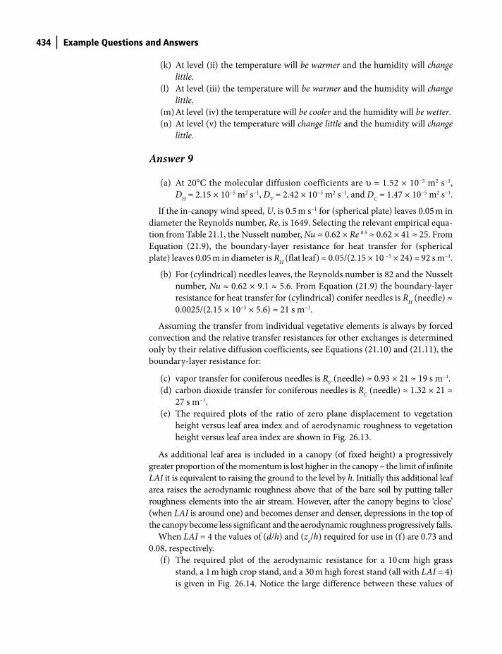
434 Example Questions and Answers
(k) At level (ii) the temperature will be warmer and the humidity will change
little.
(l) At level (iii) the temperature will be warmer and the humidity will change
little.
(m) At level (iv) the temperature will be cooler and the humidity will be wetter.
(n) At level (v) the temperature will change little and the humidity will change
little.
Answer 9
(a) At 20°C the molecular diffusion coefficients are υ = 1.52 × 10⁻⁵ m2 s−1,
DH = 2.15 × 10⁻⁵ m2 s−1, D
V = 2.42 × 10⁻⁵ m2 s−1, and D
C = 1.47 × 10⁻⁵ m2 s−1.
If the in-canopy wind speed, U, is 0.5 m s−1 for (spherical plate) leaves 0.05 m in
diameter the Reynolds number, Re, is 1649. Selecting the relevant empirical equa-
tion from Table 21.1, the Nusselt number, Nu ≈ 0.62 × Re 0.5 ≈ 0.62 × 41 ≈ 25. From
Equation (21.9), the boundary-layer resistance for heat transfer for (spherical
plate) leaves 0.05 m in diameter is RH (flat leaf) ≈ 0.05/(2.15 × 10 −5 × 24) ≈ 92 s m−1.
(b) For (cylindrical) needles leaves, the Reynolds number is 82 and the Nusselt
number, Nu ≈ 0.62 × 9.1 ≈ 5.6. From Equation (21.9) the boundary-layer
resistance for heat transfer for (cylindrical) conifer needles is RH (needle) ≈
0.0025/(2.15 × 10−5 × 5.6) ≈ 21 s m−1.
Assuming the transfer from individual vegetative elements is always by forced
convection and the relative transfer resistances for other exchanges is determined
only by their relative diffusion coefficients, see Equations (21.10) and (21.11), the
boundary-layer resistance for:
(c) vapor transfer for coniferous needles is RV (needle) ≈ 0.93 × 21 ≈ 19 s m−1.
(d) carbon dioxide transfer for coniferous needles is RC (needle) ≈ 1.32 × 21 ≈
27 s m−1.
(e) The required plots of the ratio of zero plane displacement to vegetation
height versus leaf area index and of aerodynamic roughness to vegetation
height versus leaf area index are shown in Fig. 26.13.
As additional leaf area is included in a canopy (of fixed height) a progressively
greater proportion of the momentum is lost higher in the canopy – the limit of infinite
LAI it is equivalent to raising the ground to the level by h. Initially this additional leaf
area raises the aerodynamic roughness above that of the bare soil by putting taller
roughness elements into the air stream. However, after the canopy begins to ‘close’
(when LAI is around one) and becomes denser and denser, depressions in the top of
the canopy become less significant and the aerodynamic roughness progressively falls.
When LAI = 4 the values of (d/h) and (zo/h) required for use in (f) are 0.73 and
0.08, respectively.
(f) The required plot of the aerodynamic resistance for a 10 cm high grass
stand, a 1 m high crop stand, and a 30 m high forest stand (all with LAI = 4)
is given in Fig. 26.14. Notice the large difference between these values of
Shuttleworth_c26.indd 434Shuttleworth_c26.indd 434 11/3/2011 6:37:58 PM11/3/2011 6:37:58 PM
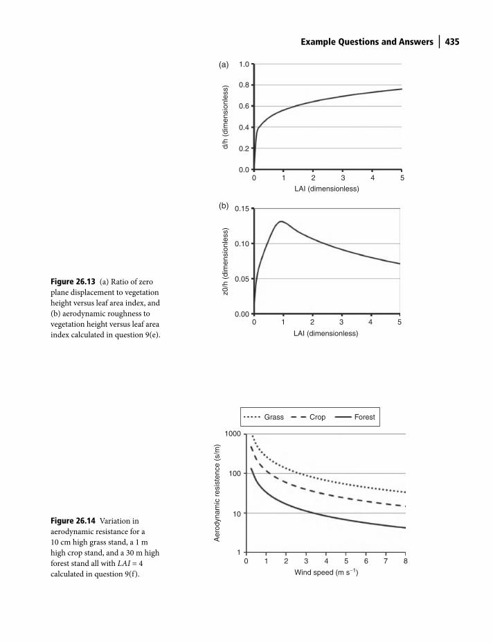
Example Questions and Answers 435
2
LAI (dimensionless)
3 4 5
1.0(a)
(b)
0.8
0.6
0.4
0.2
0.00 1
d/h
(dim
ensi
onle
ss)
2
LAI (dimensionless)
3 4 5
0.15
0.10
0.05
0.000 1
z0/h
(di
men
sion
less
)
Figure 26.13 (a) Ratio of zero
plane displacement to vegetation
height versus leaf area index, and
(b) aerodynamic roughness to
vegetation height versus leaf area
index calculated in question 9(e).
0 1 2 3 4
Wind speed (m s−1)
5 6 7 81
10
100
1000
Aer
odyn
amic
res
iste
nce
(s/m
)
Grass Crop Forest
Figure 26.14 Variation in
aerodynamic resistance for a
10 cm high grass stand, a 1 m
high crop stand, and a 30 m high
forest stand all with LAI = 4
calculated in question 9(f).
Shuttleworth_c26.indd 435Shuttleworth_c26.indd 435 11/3/2011 6:37:58 PM11/3/2011 6:37:58 PM
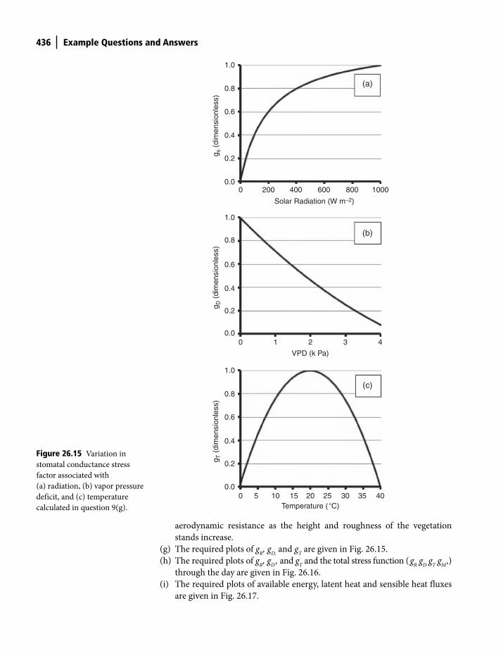
436 Example Questions and Answers
aerodynamic resistance as the height and roughness of the vegetation
stands increase.
(g) The required plots of gR, g
D, and g
T are given in Fig. 26.15.
(h) The required plots of gR, g
D , and g
T and the total stress function ( g
R g
D g
T g
M ,)
through the day are given in Fig. 26.16.
(i) The required plots of available energy, latent heat and sensible heat fluxes
are given in Fig. 26.17.
1.0
0.8
0.6
0.4
0.2
0.0
g s (
dim
ensi
onle
ss)
0 200 400 600 800 1000
1.0
0.8
0.6
0.4
0.2
0.0
g D (
dim
ensi
onle
ss)
0 1 2
VPD (k Pa)
3 4
1.0
0.8
0.6
0.4
0.2
0.0
g T (
dim
ensi
onle
ss)
0 105 20 2515Temperature ( �C)
30 4035
Solar Radiation (W m−2)
(c)
(b)
(a)
Figure 26.15 Variation in
stomatal conductance stress
factor associated with
(a) radiation, (b) vapor pressure
deficit, and (c) temperature
calculated in question 9(g).
Shuttleworth_c26.indd 436Shuttleworth_c26.indd 436 11/3/2011 6:37:58 PM11/3/2011 6:37:58 PM
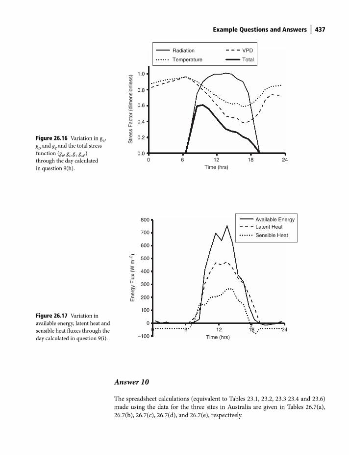
Example Questions and Answers 437
Answer 10
The spreadsheet calculations (equivalent to Tables 23.1, 23.2, 23.3 23.4 and 23.6)
made using the data for the three sites in Australia are given in Tables 26.7(a),
26.7(b), 26.7(c), 26.7(d), and 26.7(e), respectively.
1.0
0.8
0.6
0.4
0.2
0.00 6 12
Time (hrs)18 24
Radiation
Temperature
VPD
Total
Str
ess
Fac
tor
(dim
ensi
onle
ss)
Figure 26.16 Variation in gR,
gD and g
T and the total stress
function (gR, g
D g
T g
M,)
through the day calculated
in question 9(h).
800
700
600
500
400
300
200
100
0
−1000 6 12
Time (hrs)
18 24
Available EnergyLatent Heat
Sensible Heat
Ene
rgy
Flu
x (W
m−2
)
Figure 26.17 Variation in
available energy, latent heat and
sensible heat fluxes through the
day calculated in question 9(i).
Shuttleworth_c26.indd 437Shuttleworth_c26.indd 437 11/3/2011 6:37:59 PM11/3/2011 6:37:59 PM
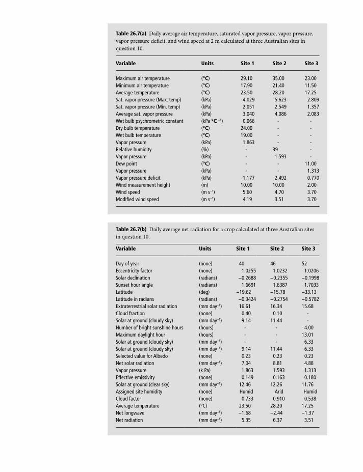
Table 26.7(b) Daily average net radiation for a crop calculated at three Australian sites
in question 10.
Variable Units Site 1 Site 2 Site 3
Day of year (none) 40 46 52Eccentricity factor (none) 1.0255 1.0232 1.0206Solar declination (radians) −0.2688 −0.2355 −0.1998Sunset hour angle (radians) 1.6691 1.6387 1.7033Latitude (deg) −19.62 −15.78 −33.13Latitude in radians (radians) −0.3424 −0.2754 −0.5782Extraterrestrial solar radiation (mm day−1) 16.61 16.34 15.68Cloud fraction (none) 0.40 0.10 -Solar at ground (cloudy sky) (mm day−1) 9.14 11.44 -Number of bright sunshine hours (hours) - - 4.00Maximum daylight hour (hours) - - 13.01Solar at ground (cloudy sky) (mm day−1) - - 6.33Solar at ground (cloudy sky) (mm day−1) 9.14 11.44 6.33Selected value for Albedo (none) 0.23 0.23 0.23Net solar radiation (mm day−1) 7.04 8.81 4.88Vapor pressure (k Pa) 1.863 1.593 1.313Effective emissivity (none) 0.149 0.163 0.180Solar at ground (clear sky) (mm day−1) 12.46 12.26 11.76Assigned site humidity (none) Humid Arid HumidCloud factor (none) 0.733 0.910 0.538Average temperature (°C) 23.50 28.20 17.25Net longwave (mm day−1) −1.68 −2.44 −1.37Net radiation (mm day−1) 5.35 6.37 3.51
Table 26.7(a) Daily average air temperature, saturated vapor pressure, vapor pressure,
vapor pressure deficit, and wind speed at 2 m calculated at three Australian sites in
question 10.
Variable Units Site 1 Site 2 Site 3
Maximum air temperature (°C) 29.10 35.00 23.00Minimum air temperature (°C) 17.90 21.40 11.50Average temperature (°C) 23.50 28.20 17.25Sat. vapor pressure (Max. temp) (kPa) 4.029 5.623 2.809Sat. vapor pressure (Min. temp) (kPa) 2.051 2.549 1.357Average sat. vapor pressure (kPa) 3.040 4.086 2.083Wet bulb psychrometric constant (kPa °C −1) 0.066 - -Dry bulb temperature (°C) 24.00 - -Wet bulb temperature (°C) 19.00 - -Vapor pressure (kPa) 1.863 - -Relative humidity (%) - 39 -Vapor pressure (kPa) - 1.593 -Dew point (°C) - - 11.00Vapor pressure (kPa) - - 1.313Vapor pressure deficit (kPa) 1.177 2.492 0.770Wind measurement height (m) 10.00 10.00 2.00Wind speed (m s−1) 5.60 4.70 3.70Modified wind speed (m s−1) 4.19 3.51 3.70
Shuttleworth_c26.indd 438Shuttleworth_c26.indd 438 11/3/2011 6:37:59 PM11/3/2011 6:37:59 PM
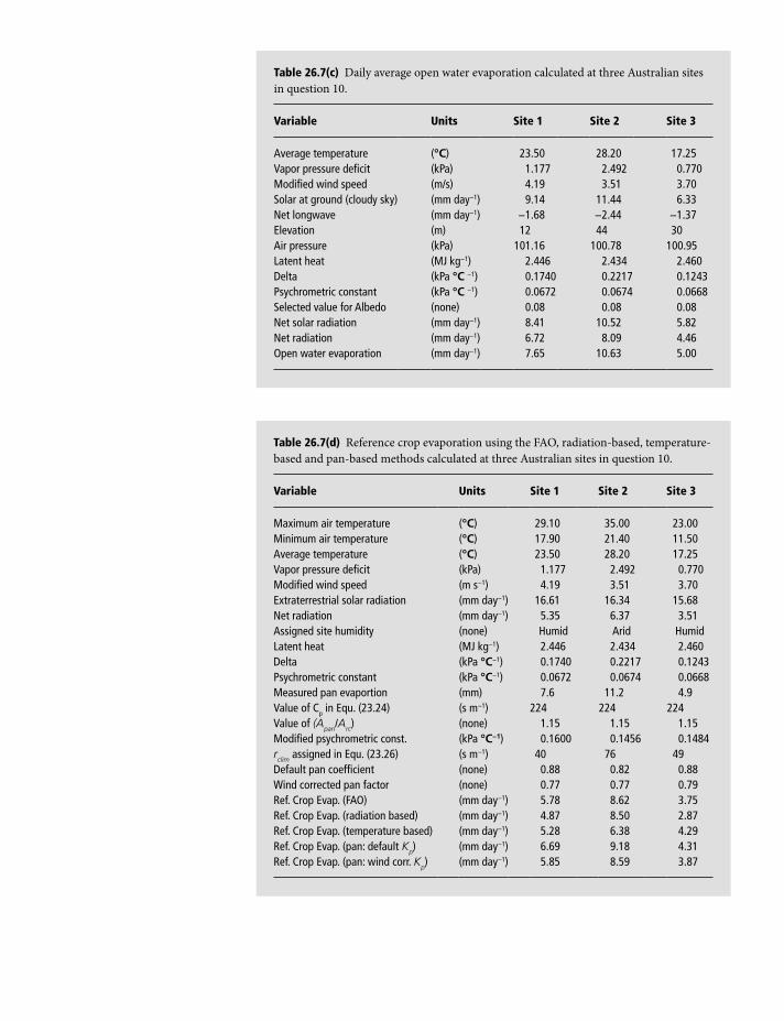
Table 26.7(c) Daily average open water evaporation calculated at three Australian sites
in question 10.
Variable Units Site 1 Site 2 Site 3
Average temperature (°C) 23.50 28.20 17.25Vapor pressure deficit (kPa) 1.177 2.492 0.770Modified wind speed (m/s) 4.19 3.51 3.70Solar at ground (cloudy sky) (mm day−1) 9.14 11.44 6.33Net longwave (mm day−1) −1.68 −2.44 −1.37Elevation (m) 12 44 30Air pressure (kPa) 101.16 100.78 100.95Latent heat (MJ kg−1) 2.446 2.434 2.460Delta (kPa °C −1) 0.1740 0.2217 0.1243Psychrometric constant (kPa °C −1) 0.0672 0.0674 0.0668Selected value for Albedo (none) 0.08 0.08 0.08Net solar radiation (mm day−1) 8.41 10.52 5.82Net radiation (mm day−1) 6.72 8.09 4.46Open water evaporation (mm day−1) 7.65 10.63 5.00
Table 26.7(d) Reference crop evaporation using the FAO, radiation-based, temperature-
based and pan-based methods calculated at three Australian sites in question 10.
Variable Units Site 1 Site 2 Site 3
Maximum air temperature (°C) 29.10 35.00 23.00Minimum air temperature (°C) 17.90 21.40 11.50Average temperature (°C) 23.50 28.20 17.25Vapor pressure deficit (kPa) 1.177 2.492 0.770Modified wind speed (m s−1) 4.19 3.51 3.70Extraterrestrial solar radiation (mm day−1) 16.61 16.34 15.68Net radiation (mm day−1) 5.35 6.37 3.51Assigned site humidity (none) Humid Arid HumidLatent heat (MJ kg−1) 2.446 2.434 2.460Delta (kPa °C−1) 0.1740 0.2217 0.1243Psychrometric constant (kPa °C−1) 0.0672 0.0674 0.0668Measured pan evaportion (mm) 7.6 11.2 4.9Value of Cp in Equ. (23.24) (s m−1) 224 224 224Value of (Apan/Arc) (none) 1.15 1.15 1.15Modified psychrometric const. (kPa °C−1) 0.1600 0.1456 0.1484rclim assigned in Equ. (23.26) (s m−1) 40 76 49Default pan coefficient (none) 0.88 0.82 0.88Wind corrected pan factor (none) 0.77 0.77 0.79Ref. Crop Evap. (FAO) (mm day−1) 5.78 8.62 3.75Ref. Crop Evap. (radiation based) (mm day−1) 4.87 8.50 2.87Ref. Crop Evap. (temperature based) (mm day−1) 5.28 6.38 4.29Ref. Crop Evap. (pan: default Kp) (mm day−1) 6.69 9.18 4.31Ref. Crop Evap. (pan: wind corr. Kp) (mm day−1) 5.85 8.59 3.87
Shuttleworth_c26.indd 439Shuttleworth_c26.indd 439 11/3/2011 6:38:00 PM11/3/2011 6:38:00 PM
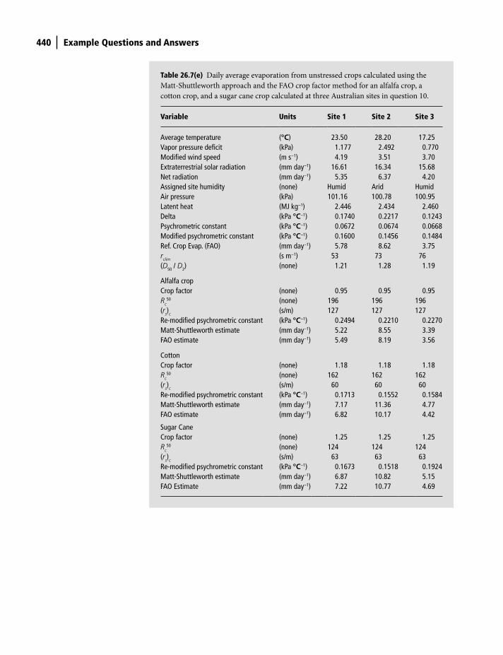
440 Example Questions and Answers
Table 26.7(e) Daily average evaporation from unstressed crops calculated using the
Matt-Shuttleworth approach and the FAO crop factor method for an alfalfa crop, a
cotton crop, and a sugar cane crop calculated at three Australian sites in question 10.
Variable Units Site 1 Site 2 Site 3
Average temperature (°C) 23.50 28.20 17.25Vapor pressure deficit (kPa) 1.177 2.492 0.770Modified wind speed (m s−1) 4.19 3.51 3.70Extraterrestrial solar radiation (mm day−1) 16.61 16.34 15.68Net radiation (mm day−1) 5.35 6.37 4.20Assigned site humidity (none) Humid Arid HumidAir pressure (kPa) 101.16 100.78 100.95Latent heat (MJ kg−1) 2.446 2.434 2.460Delta (kPa °C−1) 0.1740 0.2217 0.1243Psychrometric constant (kPa °C−1) 0.0672 0.0674 0.0668Modified psychrometric constant (kPa °C−1) 0.1600 0.1456 0.1484Ref. Crop Evap. (FAO) (mm day−1) 5.78 8.62 3.75rclim (s m−1) 53 73 76(D50 / D2) (none) 1.21 1.28 1.19
Alfalfa cropCrop factor (none) 0.95 0.95 0.95Rc
50 (none) 196 196 196(rs)c (s/m) 127 127 127Re-modified psychrometric constant (kPa °C−1) 0.2494 0.2210 0.2270Matt-Shuttleworth estimate (mm day−1) 5.22 8.55 3.39FAO estimate (mm day−1) 5.49 8.19 3.56
CottonCrop factor (none) 1.18 1.18 1.18Rc
50 (none) 162 162 162(rs)c (s/m) 60 60 60Re-modified psychrometric constant (kPa °C−1) 0.1713 0.1552 0.1584Matt-Shuttleworth estimate (mm day−1) 7.17 11.36 4.77FAO estimate (mm day−1) 6.82 10.17 4.42
Sugar CaneCrop factor (none) 1.25 1.25 1.25Rc
50 (none) 124 124 124(rs)c (s/m) 63 63 63Re-modified psychrometric constant (kPa °C−1) 0.1673 0.1518 0.1924Matt-Shuttleworth estimate (mm day−1) 6.87 10.82 5.15FAO Estimate (mm day−1) 7.22 10.77 4.69
Shuttleworth_c26.indd 440Shuttleworth_c26.indd 440 11/3/2011 6:38:00 PM11/3/2011 6:38:00 PM

Terrestrial Hydrometeorology, First Edition. W. James Shuttleworth.
© 2012 John Wiley & Sons, Ltd. Published 2012 by John Wiley & Sons, Ltd.
Index
absorptivity 51
AIRS instrument 172
atmospheric boundary layer (ABL)
atmospheric variables in 223
daytime profiles 261–3, 264, 265
diurnal evolution, over land,
under clear sky
conditions 260–1, 261
entrainment layer 260
equations of atmospheric flow
in 231–47
equations of turbulent flow
in 248–58
exchange processes 301–6, 302, 304
feedback processes, modeling 316,
327, 328, 331
higher order moments 265–75
inversion layer 260
mixed layer 260
nature and evolution of 259–61,
260, 261
nighttime profiles 263–5
resistance 302–6
structure 259–60
surface layer 259
turbulent flux at 223
virtual potential temperature
in 31–3
accretion 143
actual daily total solar radiation 59
adiabatic atmosphere 33
adiabatic lapse rates 27–9
dry 27–8
environmental 28–9
moist 28
advected energy 41
advective (mean) flux 225–9
aerodynamic resistance 289, 296–9
aerosols 131
sources 131aggregation 143
AIRS precipitation product 172
Aitken Nuclei 131
albedo of natural surface 52, 52for different surfaces 53variation with solar altitude 52,
53, 54
Amazonian deforestation 366
Andres Mountains 125
anemometer 214
annual precipitation 177
Antarctica 9
anthroposphere, features of 10–11
Archimedes principle 32
areal mean precipitation,
calculation 200–4
areal reduction factors (ARFs)
205–7, 207
Asian-Australian monsoon
system 118, 119, 383
atmosphere
circulation 7, 7
composition 5, 6
features of 5–7, 7
variance 7
water vapor in 14–24
atmospheric circulation, global scale
influences on 107–25, 108
atmospheric stability 32–4, 34
static stability parameter 32–3
atmospheric water vapor 14–24
conservation 244–5
content 15
residence time 3, 6–7
autocorrelation 187
available energy 41
averaging rules for time-dependent
variables 218Avogadro’s number 16
Azores High 123
Ball-Berry equation 368, 369
Bayesian inversion method 173
Bergeron-Findeisen process 134, 143,
144, 146, 147, 147
big-leaf assumption
of canopy resistance 312–13
of plant–atmosphere
interactions 316, 364
biochemical energy storage 40–1
biosphere, features of 10
blackbody 49
blackbody radiation laws 49–51, 50
blending height 37
bluff body transfer 302, 303, 319
‘boil off ’ rate 19
BOREAS experiment 390
Boussinesq approximation 249–50,
252, 265
Bowen ratio/energy budget
measuring method 45–6,
83–5, 85, 86
Boyle’s Law 16
Budyko Bucket model 361, 361, 364
buoyant acceleration 32–3
Campbell-Stokes recorder 78, 78
canopy capacity 324
Note: Page references in italics refer to Figures; those in bold refer to Tables
Shuttleworth_bindex.indd 441Shuttleworth_bindex.indd 441 11/3/2011 5:39:12 PM11/3/2011 5:39:12 PM
442 Index
canopy processes 300–14
canopy resistances 300–14
big leaf approach 312–13
energy budget of dry canopy
311–14, 312, 313
energy budget of dry leaf 310–11
shelter factors 306–8, 306
stomatal resistance 308–10, 309
capacitance probes 91
carbon cycle, impact of change to 11
carbon dioxide, hydroclimate changes
and 110
Cartesian Grid 102, 102
CENTURY model 370
Charles’s law 16
chlorinated fluorocarbons (CFCs) 11
cirrus 140
climate prediction 100
cloud condensation nuclei (CCN) 128,
131–2
cloud cover, daily estimates 77–8
cloud droplets
collection efficiency of 144, 145
collision efficiency of 144
collision of 144–5, 145
size, concentration and terminal
velocity 133, 133cloud factor 61
in arid conditions 62
in humid conditions 62
cloud formation 128–41
cloud droplet size, concentration
and terminal velocity 133, 133extratropical fronts and
cyclones 138–40, 139
Foehn effect 136–8, 137, 138
ice in 134–5
mechanisms 129–30, 129
processes 135–40
requirements 128
saturated vapor pressure of curved
surfaces 132–3, 132
temperature ranges and
constituents 134
thermal convection 135–6, 136
cloud genera 140–1, 141cloud indices 171
cloud type, rain production by 148–9
coalescence 143
coalescence efficiency 144
cold clouds 134
cold front 138
collection efficiency of cloud
droplets 144, 145
collision efficiency of cloud
droplets 144
collision of cloud droplets 144–5, 145
Community Land Model
(CLM) 371–2
conditional probabilities 195, 196
conservation laws 101, 231
conservation of atmospheric
moisture 244–5
conservation of energy 231, 245–6,
245, 257conservation of mass 231, 243–4,
245, 257conservation of moisture 245, 254,
255, 257conservation of momentum 231,
234–42, 245, 257axis-specific forces 239–42, 240
combined momentum forces 242
pressure forces 235–6, 235
in turbulent ABL 252–4
viscous flow in fluids 236–9, 238
conservation of scalar quantity 245,
246, 254, 255, 257contact nucleation 134
continental land cover 110
continental topography 109
continental water balance,
estimated 5Continuity Equation for mass of
air 243
convective cloud 130
conventional frequency
distribution 193
Coriolis force 113, 114, 240
correlation of variables 221–3, 223
correlogram 187
counter gradient flow 282
cryosphere, features of 9
cumulative percentage
deviations 183–4, 185
cumulonimbus cloud 140, 147
cumulus 128, 140
cyclones 119–20, 120, 139–40, 139
daily average values of weather
variables 335–8
net radiation 337–8, 339
temperature, humidity and wind
speed 335–7, 337daily estimates of evaporation 334–55
Matt-Shuttleworth approach
348–53, 352, 354, 392
open water evaporation 339–41,
341reference crop
evapotranspiration 341–2, 348evaporation pan-based estimation
of 346–8
Penman-Monteith equation
estimation of 342–3
radiation-based estimation
of 344–5, 345
temperature-based
estimation 345–6
vs SVATS 334
unstressed vegetation 348–53, 352,
354, 392
water stressed vegetation 353–5
daily precipitation 180, 181
Dalton’s law of partial pressures 16
damping depth 73, 74, 75
day length 57
decomposed variables, averaging
of 217–19
deforestation 110
density of soil 69–70, 69design storms 205–7
dew 152–3
dew point hygrometer 21
dew point of air 21
dimensionless gradients 290–2
of specific humidity 291, 292, 295
of virtual potential
temperature 291–2
of wind speed 290
dimensionless measure
of atmospheric stability 289
of buoyant production 291,
292, 293
dimensionless prognostic equation for
TKE 290
divergence equation for turbulent
fluctuations 250
divergence of net radiation flux 246
Doldrums, the 112
Doppler effect 169
drag coefficient 302, 304
drizzle 149
Shuttleworth_bindex.indd 442Shuttleworth_bindex.indd 442 11/3/2011 5:39:13 PM11/3/2011 5:39:13 PM
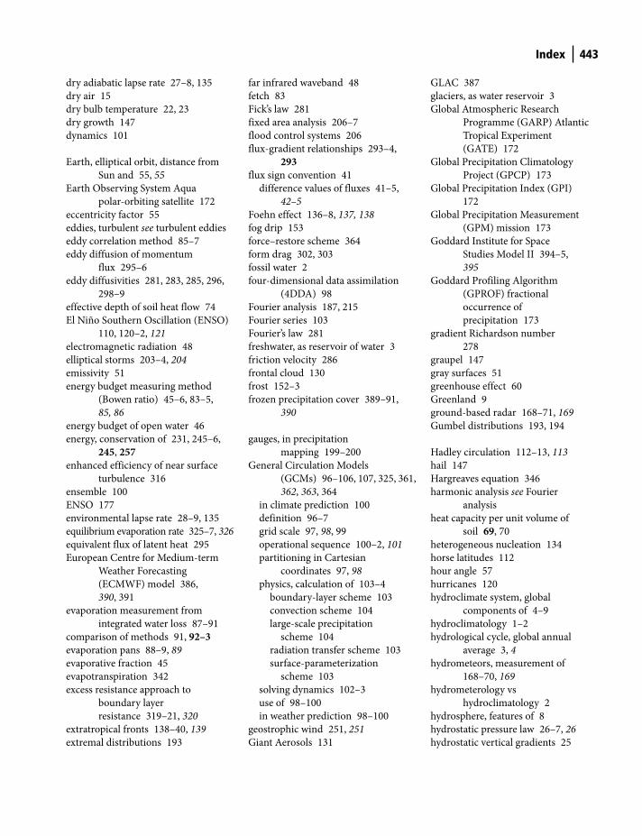
Index 443
dry adiabatic lapse rate 27–8, 135
dry air 15
dry bulb temperature 22, 23
dry growth 147
dynamics 101
Earth, elliptical orbit, distance from
Sun and 55, 55
Earth Observing System Aqua
polar-orbiting satellite 172
eccentricity factor 55
eddies, turbulent see turbulent eddies
eddy correlation method 85–7
eddy diffusion of momentum
flux 295–6
eddy diffusivities 281, 283, 285, 296,
298–9
effective depth of soil heat flow 74
El Niño Southern Oscillation (ENSO)
110, 120–2, 121
electromagnetic radiation 48
elliptical storms 203–4, 204
emissivity 51
energy budget measuring method
(Bowen ratio) 45–6, 83–5,
85, 86
energy budget of open water 46
energy, conservation of 231, 245–6,
245, 257enhanced efficiency of near surface
turbulence 316
ensemble 100
ENSO 177
environmental lapse rate 28–9, 135
equilibrium evaporation rate 325–7, 326
equivalent flux of latent heat 295
European Centre for Medium-term
Weather Forecasting
(ECMWF) model 386,
390, 391
evaporation measurement from
integrated water loss 87–91
comparison of methods 91, 92–3evaporation pans 88–9, 89
evaporative fraction 45
evapotranspiration 342
excess resistance approach to
boundary layer
resistance 319–21, 320
extratropical fronts 138–40, 139
extremal distributions 193
far infrared waveband 48
fetch 83
Fick’s law 281
fixed area analysis 206–7
flood control systems 206
flux-gradient relationships 293–4,
293flux sign convention 41
difference values of fluxes 41–5,
42–5
Foehn effect 136–8, 137, 138
fog drip 153
force–restore scheme 364
form drag 302, 303
fossil water 2
four-dimensional data assimilation
(4DDA) 98
Fourier analysis 187, 215
Fourier series 103
Fourier’s law 281
freshwater, as reservoir of water 3
friction velocity 286
frontal cloud 130
frost 152–3
frozen precipitation cover 389–91,
390
gauges, in precipitation
mapping 199–200
General Circulation Models
(GCMs) 96–106, 107, 325, 361,
362, 363, 364
in climate prediction 100
definition 96–7
grid scale 97, 98, 99
operational sequence 100–2, 101
partitioning in Cartesian
coordinates 97, 98
physics, calculation of 103–4
boundary-layer scheme 103
convection scheme 104
large-scale precipitation
scheme 104
radiation transfer scheme 103
surface-parameterization
scheme 103
solving dynamics 102–3
use of 98–100
in weather prediction 98–100
geostrophic wind 251, 251
Giant Aerosols 131
GLAC 387
glaciers, as water reservoir 3
Global Atmospheric Research
Programme (GARP) Atlantic
Tropical Experiment
(GATE) 172
Global Precipitation Climatology
Project (GPCP) 173
Global Precipitation Index (GPI)
172
Global Precipitation Measurement
(GPM) mission 173
Goddard Institute for Space
Studies Model II 394–5,
395
Goddard Profiling Algorithm
(GPROF) fractional
occurrence of
precipitation 173
gradient Richardson number
278
graupel 147
gray surfaces 51
greenhouse effect 60
Greenland 9
ground-based radar 168–71, 169
Gumbel distributions 193, 194
Hadley circulation 112–13, 113
hail 147
Hargreaves equation 346
harmonic analysis see Fourier
analysis
heat capacity per unit volume of
soil 69, 70
heterogeneous nucleation 134
horse latitudes 112
hour angle 57
hurricanes 120
hydroclimate system, global
components of 4–9
hydroclimatology 1–2
hydrological cycle, global annual
average 3, 4
hydrometeors, measurement of
168–70, 169
hydrometerology vs
hydroclimatology 2
hydrosphere, features of 8
hydrostatic pressure law 26–7, 26
hydrostatic vertical gradients 25
Shuttleworth_bindex.indd 443Shuttleworth_bindex.indd 443 11/3/2011 5:39:13 PM11/3/2011 5:39:13 PM
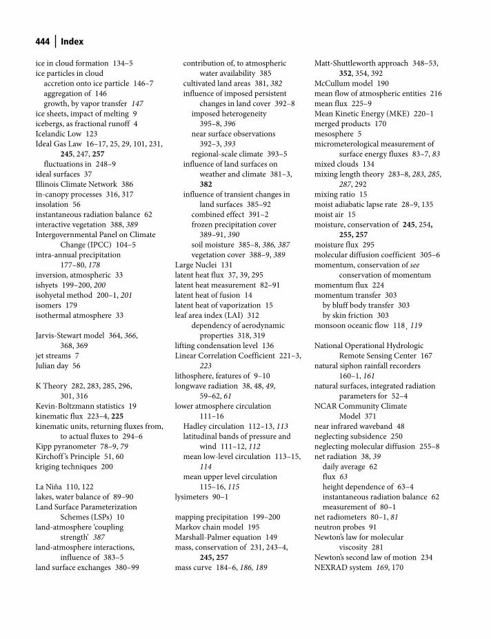
444 Index
ice in cloud formation 134–5
ice particles in cloud
accretion onto ice particle 146–7
aggregation of 146
growth, by vapor transfer 147
ice sheets, impact of melting 9
icebergs, as fractional runoff 4
Icelandic Low 123
Ideal Gas Law 16–17, 25, 29, 101, 231,
245, 247, 257fluctuations in 248–9
ideal surfaces 37
Illinois Climate Network 386
in-canopy processes 316, 317
insolation 56
instantaneous radiation balance 62
interactive vegetation 388, 389
Intergovernmental Panel on Climate
Change (IPCC) 104–5
intra-annual precipitation
177–80, 178
inversion, atmospheric 33
ishyets 199–200, 200
isohyetal method 200–1, 201
isomers 179
isothermal atmosphere 33
Jarvis-Stewart model 364, 366,
368, 369
jet streams 7
Julian day 56
K Theory 282, 283, 285, 296,
301, 316
Kevin-Boltzmann statistics 19
kinematic flux 223–4, 225kinematic units, returning fluxes from,
to actual fluxes to 294–6
Kipp pyranometer 78–9, 79
Kirchoff ’s Principle 51, 60
kriging techniques 200
La Niña 110, 122
lakes, water balance of 89–90
Land Surface Parameterization
Schemes (LSPs) 10
land-atmosphere ‘coupling
strength’ 387
land-atmosphere interactions,
influence of 383–5
land surface exchanges 380–99
contribution of, to atmospheric
water availability 385
cultivated land areas 381, 382
influence of imposed persistent
changes in land cover 392–8
imposed heterogeneity
395–8, 396
near surface observations
392–3, 393
regional-scale climate 393–5
influence of land surfaces on
weather and climate 381–3,
382influence of transient changes in
land surfaces 385–92
combined effect 391–2
frozen precipitation cover
389–91, 390
soil moisture 385–8, 386, 387
vegetation cover 388–9, 389
Large Nuclei 131
latent heat flux 37, 39, 295
latent heat measurement 82–91
latent heat of fusion 14
latent heat of vaporization 15
leaf area index (LAI) 312
dependency of aerodynamic
properties 318, 319
lifting condensation level 136
Linear Correlation Coefficient 221–3,
223
lithosphere, features of 9–10
longwave radiation 38, 48, 49,
59–62, 61
lower atmosphere circulation
111–16
Hadley circulation 112–13, 113
latitudinal bands of pressure and
wind 111–12, 112
mean low-level circulation 113–15,
114
mean upper level circulation
115–16, 115
lysimeters 90–1
mapping precipitation 199–200
Markov chain model 195
Marshall-Palmer equation 149
mass, conservation of 231, 243–4,
245, 257mass curve 184–6, 186, 189
Matt-Shuttleworth approach 348–53,
352, 354, 392
McCullum model 190
mean flow of atmospheric entities 216
mean flux 225–9
Mean Kinetic Energy (MKE) 220–1
merged products 170
mesosphere 5
micrometerological measurement of
surface energy fluxes 83–7, 83
mixed clouds 134
mixing length theory 283–8, 283, 285,
287, 292
mixing ratio 15
moist adiabatic lapse rate 28–9, 135
moist air 15
moisture, conservation of 245, 254, 255, 257
moisture flux 295
molecular diffusion coefficient 305–6
momentum, conservation of see
conservation of momentum
momentum flux 224
momentum transfer 303
by bluff body transfer 303
by skin friction 303
monsoon oceanic flow 118¸ 119
National Operational Hydrologic
Remote Sensing Center 167
natural siphon rainfall recorders
160–1, 161
natural surfaces, integrated radiation
parameters for 52–4
NCAR Community Climate
Model 371
near infrared waveband 48
neglecting subsidence 250
neglecting molecular diffusion 255–8
net radiation 38, 39
daily average 62
flux 63
height dependence of 63–4
instantaneous radiation balance 62
measurement of 80–1
net radiometers 80–1, 81
neutron probes 91
Newton’s law for molecular
viscosity 281
Newton’s second law of motion 234
NEXRAD system 169, 170
Shuttleworth_bindex.indd 444Shuttleworth_bindex.indd 444 11/3/2011 5:39:13 PM11/3/2011 5:39:13 PM
Index 445
Nipher gauge 159
nitrogen, atmospheric 6
Noah land surface model 389
North American Monsoon experiment
(NAME) 383
North American Monsoon System
(NAMS) 118
North Atlantic Oscilllation
(NAO) 123, 123
numeric filters 187
Numerical Weather Prediction
(NWP) 98, 99–100
Nusselt number 303–4, 304
relationship with Reynolds
number 305
Obukov length 292–3, 329
ocean mixed layer 116
ocean to continent surface
exchanges 109
oceanic influences on continental
hydroclimate 118–23
El Nino Southern Oscillation
(ENSO) 110, 120–2, 121
monsoon flow 118¸ 119
North Atlantic Oscilllation
(NAO) 123, 123
Pacific Decadal Oscillation
(PDO) 110, 122, 122
tropical cyclones 119–20, 120
oceanic circulation 110, 116–18, 117
oceanic movement, response time 7
Ohm’s Law 297
open water, energy budget of 46
open water evaporation 46
daily estimates of 339–41, 341outward longwave radiation
(OLR) 172
oxygen, atmospheric 6
ozone 6
Pacific Decadal Oscillation
(PDO) 110, 122, 122
paired catchments 89–90, 90
pan coefficients 89
pan factor 346
parameterizations 216
pauses in atmospheric temperature, 5
Pearson distributions 193, 194
Penman-Monteith equation 316, 324,
329, 339–40, 349, 350, 353, 361
calculation of evaporation 346–7
estimation of reference crop
evapotranspiration 342–3
single leaf 311
whole-canopy 312, 313–14
Pennsylvania State-National Center
for Atmospheric Research
Mesoscale Model (MM5)
393–4, 394
Penpan equation 346–8
permafrost as water reservoir 3
PERSIANN precipitation product 172
photoelectric pyranometers 79, 80
Photosynthetically Active Radiation
(PAR) 54
physical energy storage 40
pie diagrams 179
Planck’s Law 50
planetary interrelationships 109
pluviometric coefficients 179
Plynlimon paired catchments 90, 90
point area precipitation
relationships 206
by duration 205, 206
by return period 205, 205
polar diagrams 179
potential rate of evaporation 328, 341
potential temperature 25, 30
precipitable water 124, 124
precipitation
cloud type and 148–9
extreme, statistics of 190–5
forms 149, 149frozen, types 151
rates and kinetic energy 151
seasonal, time of onset 180
precipitation analysis in
space 198–211
precipitation analysis in time 176–97
precipitation climatology 176,
177–80
annual variations 177
daily variations 180, 181
intra-annual variations 177–80, 178
precipitation, formation of 143–53,
148
in cold clouds 146
in mixed clouds 146–7
in warm clouds 144–6, 145
precipitation frequency
distribution 192–3, 192
precipitation intensity-duration
relationships 189–90, 190, 191
precipitation measurement and
observation 155–75
precipitation oscillations 186–7
precipitation recycling 385
precipitation trends 181–6, 182, 183
cumulative percentage
deviations 183–4, 185
mass curve 184–6, 186, 189
running means 182–3, 184
Priestley-Taylor equation 345, 351
PRISM methodology 383
probability distributions 193–5
conventional frequency 193
Gumbel distributions 193, 194
Pearson distributions 193, 194
extremal distributions 193
transformal distributions 193
probable maximum precipitation
(PMP) 207–9, 209
prognostic equations 247, 258
for turbulent departures 265–9
for turbulent kinetic energy
269–71, 270, 271, 272
for variance of moisture and
heat 271–5, 274, 275
of velocity components 279, 280
psychrometric constant 23, 335
pyrgeometers 81, 81
quantum sensors 79
radar
ground-based, precipitation
estimation 155
spaceborne 173
radar reflectivity factor 170
radiant energy, latitudinal imbalance
in 110–11, 111
radiation spectrum 48, 49
radiation exchange 51
radiation properties 51
radioactively active gases 58
radioactively active gases, absorption
spectra of 60
rain gauges 155, 156–65
areal representativeness of
measurements 162–4, 163
design specifications 156, 156designs 160–2
Shuttleworth_bindex.indd 445Shuttleworth_bindex.indd 445 11/3/2011 5:39:13 PM11/3/2011 5:39:13 PM
446 Index
rain gauges (cont’d )
instrumental errors 157
inter-gauge correlations 164, 165minimum gauge densities 164, 165site and location errors
157–60, 158
tipping bucket design 157
turbulence minimisation
158–9, 159
turf wall construction 158–9, 159
raindrop
shape 150, 150
size distribution 149, 149
rainfall see entries under precipitation
Rayleigh scattering 58, 170
reanalysis data 100
reciprocal-distance-squared
methods 200, 201, 202
reference crop evapotranspiration
341–2, 348
evaporation pan-based estimation
of 346–8
Penman-Monteith equation
estimation of 342–3
radiation-based estimation
of 344–5, 345
temperature-based
estimation 345–6
reference level 38
reflectivity 51
relative humidity 20
remote sensing, precipitation
estimation 155–5
resistance analogues 296–9
Reynolds averaging 219, 231, 248, 249,
252, 253, 255, 267
Reynolds number 300, 301
relationship with Nusselt
number 304, 305Richards equation 370, 372
Richardson number 277–9, 279,
292, 293
riming 143
Rocky Mountains 125
running means 182–3, 184
runoff ratios 4
Rutter model of wet canopy
evaporation 323–5, 324
salt water, as reservoir of water 2
saturated vapor pressure 18–20, 18, 20
saturation, measures of 20–1
scalar quantity, conservation of 245,
246, 254, 255, 257sea-surface temperature (SST)
116, 117
Seasonality Index 179
sensible heat flux 37–8, 39, 224
sensible heat measurement 82–91
shelter factors 306–8, 306, 317
Sherwood number 305
Simple Biosphere Model (SiB) 10, 11
siphon and chart recorders 160
skin friction 301, 319
Slab Model 280–1, 281, 328
sleet, formation 152
SNOTEL network 168, 168
snow board 166
snow courses 167, 167
snow formation 152
snow pads 167–8
snow pillows 167–8
snowflake formation 146
snowfall measurement 165–8
inverted funnel method 166
radioactive methods 167
SNOTEL network 168, 168
snow courses 167, 167
snow pads or snow pillows 167–8
using gauges 165–6
using snow board 166
satellite systems 171–3
cloud mapping and
characterization 171–2
passive measurement of cloud
properties 172–3
spaceborne radar 173
soil density 69–70, 69soil heat flow, formal
description 71–2, 72
damping depth and 74
soil heat flux 39–40
measurement 81–2, 82
soil heat flux plates 81–2, 82
soil moisture 385–8, 386, 387
depletion 91, 91
soil surface temperature 66–7
surface energy balance and 67
thermal waves in 72–5, 73
Soil Vegetation Atmosphere Transfer
Schemes (SVATs) 10, 11, 334,
359–74, 388, 391
basis and origin of land-surface
sub-models 359–62
developing realism in 362–73
greening of 369
ongoing developments of land
surface sub-models 370–3,
371, 373
plot scale, one-dimensional
‘micrometerological’
models 364–7, 364
‘two stream’ approximation 365
representation
of carbon dioxide exchange
368–70, 369
of hydrological processes
367–70, 367
requirements 360soil
homogeneous, thermal waves
in 72–5, 73
thermal properties 68–71, 69solar (shortwave) radiation 48, 49
Solar Constant 36, 54
solar declination 56
solar energy impact, latitudinal
differences in 109
solar radiation 38
actual, at the ground 59
atmospheric attenuation of 58–9, 58
maximum at ground 56–7
maximum at top of
atmosphere 54–6
measurement of 77–80
solar zenith angle 56
South America
Amazon River, ‘river breeze’
effects 8
Andes 9
spaceborne radar 173
spatial correlation of
precipitation 209–11, 210
spatial organization of
precipitation 203–4
specific heat of soil 69, 70
specific humidity of air 15
spectral gap 12, 216
spectral grid 102, 102
spontaneous nucleation 134
stability corrections 289
standard deviation of atmospheric
variable 219–20
Shuttleworth_bindex.indd 446Shuttleworth_bindex.indd 446 11/3/2011 5:39:13 PM11/3/2011 5:39:13 PM
Index 447
state variables 101
static stability parameter 32–3
statistics of extremes 190–5
Stefan-Boltzmann constant 338
Stefan-Boltzmann Law 50, 59
stomatal resistance 308–10, 309
per unit area of leaf 309, 310
reciprocal of area-weighted
average 309–10
storm centered analysis 206
stratocumulus clouds 128
stratosphere 5
stratus 140
subadiabatic atmosphere 33
subsidence 250
substratum heat flux 40
subsurface soil temperatures 67–8,
68, 69
summation convention 232
Sun—Earth distance 55, 55
sunset hour angle 57
superadiabatic atmosphere 33
surface emissivity of natural
surface 52
for different surfaces 53surface energy fluxes 36–47
units 36
energy balance of ideal
surface 38–45, 38
surface layer scaling 289–99
surface mixing cloud 130
surface, net radiation at 62–3
system signature
of precipitation 187–8, 189
of storm 176
Taylor expansion 235
Television Infrared Operational
Satellite (TIROS) Operational
Vertical Sounder (TOVS)
instruments 172
terrestrial radiation 48–65
net radiation at surface 62–3
Theissen method 200, 202–3,
204, 207
thermal conductivity of soil 69, 70
thermal diffusivity of soil 69, 71
thermocline 116
thermoelectric pyranometers 78–9, 79
thermohaline circulation 118
thermosphere 5
time-average of weather, climate
as 1–2
time-domain reflectometer sensors 91
time rate of change in a fluid 232–4, 233
tipping bucket rain gauge 157,
161–2, 162
TOP model 370
topography, effect of, on convection
and precipitations 383–5
TOVS precipitation estimate 172
Trade Winds 112
transformal distributions 193
transmissivity 51
Triangle method 200, 202, 203
Tropical Rainfall Measuring mission
(TRMM) 173
tropical storms 119–20, 120
troposphere 5
turbulence, atmospheric
advective and turbulent fluxes
225–9, 227–9
averaging of decomposed
variables 217–19
kinematic flux 223–4, 225linear correlation coefficient
221–3, 223
mean and fluctuating
components 216–17, 217, 217measures of strength of 220–1
signature and spectrum of 213–16,
214, 215
turbulent flux 223
turbulent closure 279–80
local 280
local, first order 281–2, 282, 287–8
low order 280–1
nonlocal 280
turbulent eddies 85–7, 87, 214, 214,
223, 225–9
divergence 250
turbulent flux see turbulent eddies
turbulent intensity 220
turbulent kinematic flux of water
vapor 284
Turbulent Kinetic Energy (TKE) 221
prognostic equations for 269–71,
270, 271, 272
typhoons 120
ultraviolet radiation 6
ultraviolet waveband 48
United Nations Environment
Programme (UNEP) 104
United Nations Framework
Convention on Climate
Change 104
universal gas constant 16
USA
Great Lakes, ‘lake effect’ 8
Rocky Mountains 9
vapor pressure deficit 20, 336
vapor pressure of air, measuring
21–3
vapor pressure of moist air 17
variance of atmospheric
variable 219–20
vector algebra 232
vegetation cover 388–9, 389
vertical gradients in
atmosphere 25–34
vertical pressure and temperature
gradients, atmospheric
29–30, 30
virtual potential temperature
26, 224
atmospheric 31–2, 31
virtual temperature 17–18, 26
visible waveband 48
volcanic pollution 110
von Kármán constant 286
warm clouds 134
warm front 138, 139
water balance equation 88, 88
water cycle, global 1–13
water molecule capture rate by water
surface 19
water reservoirs, estimated sizes 2, 3water vapor flux 224
water vapor in the atmosphere 123–5,
124, 125
watersheds, water balance of 89–90
wavelength, separation of 48, 49
weather prediction 98–100
Weather Research and Forecasting
(WRF) model 389
Wein’s Law 50
wet bulb depression 23
wet bulb equation 23
wet bulb temperature 22, 23
wetting errors 157
Shuttleworth_bindex.indd 447Shuttleworth_bindex.indd 447 11/3/2011 5:39:13 PM11/3/2011 5:39:13 PM

448 Index
whole-canopy interactions 316–33
aerodynamics and canopy
structure 317–19, 318
equilibrium evaporation 325–7, 326
evaporation into an unsaturated
atmosphere 327–32, 328,
330, 331
roughness sublayer 321–3
wet canopies 323–5
World Meterological Organization
(WMO) 98, 104
recommended rain gauge
densities 164, 165World Weather Watch (WWW) 98
zero flux plane 91
zero identity 252
zero order closure 280
zero plane displacement 286
Z-R relationship 170
Shuttleworth_bindex.indd 448Shuttleworth_bindex.indd 448 11/3/2011 5:39:13 PM11/3/2011 5:39:13 PM