
Terrain Metrics and Landscape Characterization from Bathymetric Data ... · PDF fileTerrain...
46
i Terrain Metrics and Landscape Characterization from Bathymetric Data: SAGA GIS Methods and Command Sequences
Transcript of Terrain Metrics and Landscape Characterization from Bathymetric Data ... · PDF fileTerrain...
i
Terrain Metrics and Landscape Characterization from Bathymetric Data:
SAGA GIS Methods and Command Sequences

ii
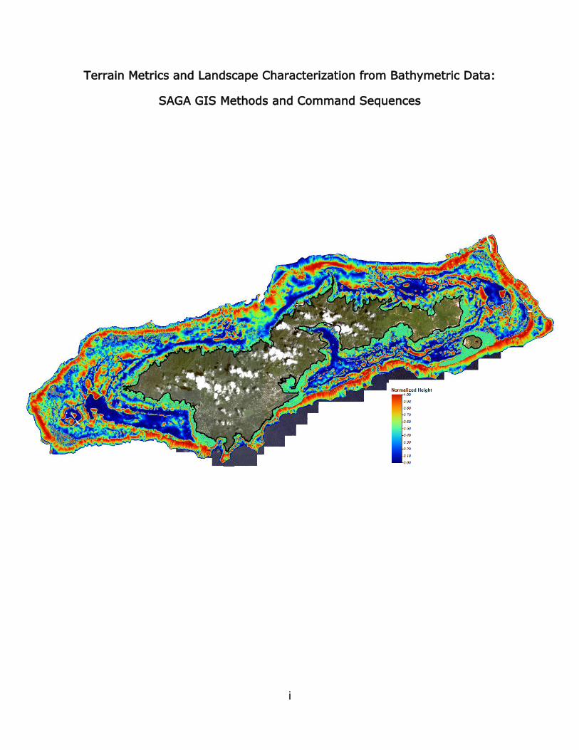
On the Cover: Ikonos mosaic sourced from: https://data.noaa.gov/dataset/tutuila-island-ikonos-imagery-
ikonos-imagery-for-american-samoa16efa
SAGA GIS Normalized Height derived from merged Ikonos and multibeam bathymetry
http://www.soest.hawaii.edu/pibhmc/pibhmc_amsamoa_tutuila_bathy.htm
Prepared by:
Russell Watkins, PhD.
Geospatial Consultant and 3K3 LLC affiliate
Organizational support provided by:
Jeff Lower; Jay Arnold
3K3 LLC
System for Automated Geoscientific Analyses (SAGA) GIS courtesy of:
J. Böhner and O. Conrad, Institute of Geography, University of Hamburg
SAGA GIS development Community, OSGeo.org
iii
Contents
On the Cover:............................................................................................. ii
Table of Figures ......................................................................................... iv
Background ................................................................................................... 1
Organization .................................................................................................. 2
General Description of SAGA GUI ..................................................................... 3
Description of Command Sequences ................................................................. 4
Start SAGA and Import ESRI ASCII Grid data ................................................. 5
Set Grid projection, coordinate system and datum .......................................... 6
Export SAGA grid to ESRI ASCII grid format ................................................... 7
TERRAIN METRIC SEQUENCES ......................................................................... 8
Slope, Aspect and Curvature ........................................................................ 9
Convergence Index ................................................................................... 10
Morphometric Protection Index ................................................................... 12
Real Surface Area ..................................................................................... 14
Terrain Ruggedness Index (TRI) ................................................................. 15
Terrain Surface Convexity .......................................................................... 17
Terrain Surface Texture ............................................................................. 19
Topographic Position Index ........................................................................ 21
TERRAIN CLASSIFICATION SEQUENCES ......................................................... 23
Fuzzy Landform Element Classification ......................................................... 24
Grid Pattern Analysis ................................................................................. 27
Surface Specific Points ............................................................................... 29
Terrain Surface Classification ...................................................................... 30
TPI Based Landform Classification ............................................................... 32
References .................................................................................................. 34
Appendix 1: Metrics and Terrain Classification Options ...................................... 36
Reviewed but Not Selected ............................................................................ 36
Appendix 2: Evaluation of “No Data” areas and Morphometric Protection Index.... 40
iv
Table of Figures
figure 1: SAGA GUI ........................................................................................ 3
Figure 2: Start SAGA and Import ESRI ASCII Grid Data ...................................... 5
Figure 3: Set Grid Projection, Coordinate System and Datum .............................. 6
Figure 4: Export SAGA Grid to ESRI ASCII Grid Format ....................................... 7
Figure 5: Slope, Aspect and Curvature .............................................................. 9
Figure 6: Convergence Index ......................................................................... 11
Figure 7: Morphometric Protection Index ........................................................ 13
Figure 8: Real Surface Area ........................................................................... 14
Figure 9: Terrain Ruggedness Index (TRI) ....................................................... 16
Figure 10: Terrain Surface Convexity .............................................................. 18
Figure 11: Terrain Surface Texture ................................................................. 20
Figure 12: Topographic Position Index ............................................................ 22
Figure 13: Fuzzy Landform Element Classification ............................................ 26
Figure 14: Grid Pattern Analysis ..................................................................... 28
Figure 15: Surface Specific Points .................................................................. 29
Figure 16: Terrain Surface Classification ......................................................... 31
Figure 17: TPI-Based Landform Classification .................................................. 33
Figure 18: Relative Heights And Slope Positions ............................................... 38
Figure 19: a) SAGA-Generated “No Data” Area; b) Bathymetry “No Data” Area ... 40
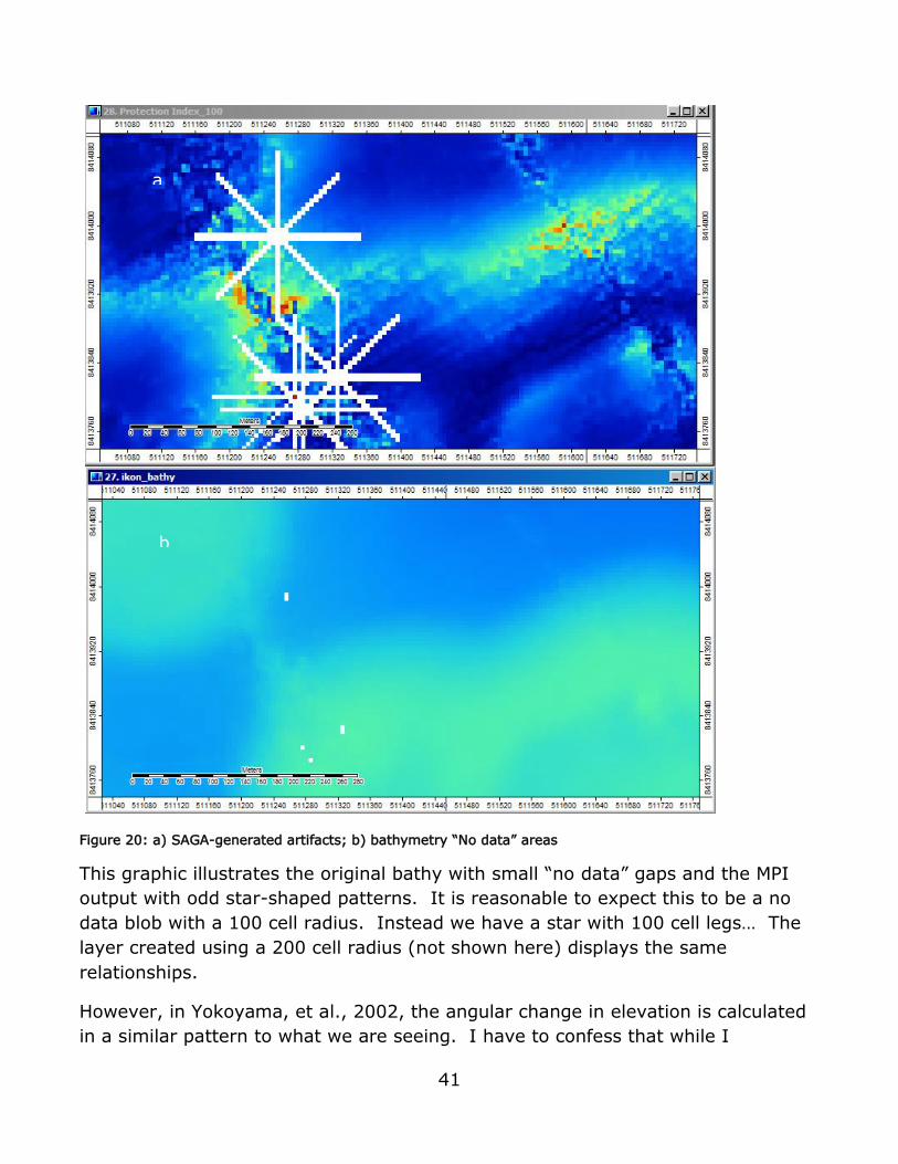
Figure 20: a) SAGA-Generated Artifacts; b) Bathymetry “No Data” Areas ............ 41

1
Background
This document is a guide to the derivation of a variety of terrain metrics and
descriptive measures of landscape composition. These metrics are to be used in
support of the “Linkages” project, which is evaluating the relationship of terrain to
fish and coral demographics in the Pacific region.
It is a “how to” document, providing command sequences, using the open source
GIS software System for Automated Geoscientific Analyses (SAGA), to generate
raster data layers of terrain metrics. SAGA was created, and is under continuous
development by researchers at the Department of Physical Geography, Hamburg,
Germany. It is distributed under the GNU General Public License (GPL), and is
available for download from http://sourceforge.net/projects/saga-gis/files/. The
project homepage is http://www.saga-gis.org/en/index.html.
Most, if not all of these metrics are available through other software packages.
However, this would require the user to learn command sequences and processes
for multiple software packages, as well as having to convert between different file
formats. The use of SAGA is a more effective and efficient approach, by providing
a comprehensive compilation of metrics, requiring only a single sequence for data
import, and allowing the user to focus on the individual metrics of interest.

2
Organization
A brief description of the SAGA GUI is provided in the course of describing the
steps to import CRED bathymetric data (in the ESRI ASCII grid file format, sourced
from the PIBHMC site). In addition, sequences are provided to set the base GRID
projection and coordinate system, as well as to EXPORT grids created in SAGA to
the ESRI ASCII grid format. Users of this document are highly encouraged to
review the SAGA User guides, Wiki and Library documentation, as well as a helpful
tutorial can be found at the following URL:
http://live.osgeo.org/en/quickstart/saga_quickstart.html
These descriptions are followed by the command sequences necessary to generate
the various metrics. The sequences are organized by module; include brief
description of the metric, either taken from SAGA documentation or from a
relevant reference, a graphic of the command hierarchy and definitions of
dependent parameters where available. A list of references for further reading is
provided at the end of the document. Example SAGA grid outputs from the
sequences listed can be seen in the SAGA GIS Terrain Metrics and Classification
Output.pptx PowerPoint presentation, which is a separate file.
3
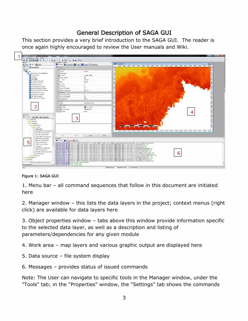
General Description of SAGA GUI
This section provides a very brief introduction to the SAGA GUI. The reader is
once again highly encouraged to review the User manuals and Wiki.
Figure 1: SAGA GUI
1. Menu bar – all command sequences that follow in this document are initiated
here
2. Manager window – this lists the data layers in the project; context menus (right
click) are available for data layers here
3. Object properties window – tabs above this window provide information specific
to the selected data layer, as well as a description and listing of
parameters/dependencies for any given module
4. Work area – map layers and various graphic output are displayed here
5. Data source – file system display
6. Messages – provides status of issued commands
Note: The User can navigate to specific tools in the Manager window, under the
"Tools" tab; in the "Properties" window, the "Settings" tab shows the commands
1
2
3
4
5
6

4
and options in the metric command sequences, while the "Description" tab
provides tool descriptions and supporting documentation
Description of Command Sequences
Sequences will take the form of a hierarchical tree. The section heading will
describe the purpose of the sequence (e.g. “Set projection of Grid”) and will
include the module name where appropriate. The primary bubble is a command
found on the Menu bar. Subsequent bubbles list the commands in order of
execution. It is assumed that the user will select or “click” on the command, so
this information is not repeated incessantly… Explanatory notes are provided
under “Note:”. Definitions/explanations of dependent parameters are provided
where needed. It should be noted that the following tree is an exception as it
describes the initial startup of SAGA and importation of data.
For each “Data Object = <create>, this will be the name of the output layer; e.g.
“Normalized Height” = <create> will yield a normalized height data layer.
5
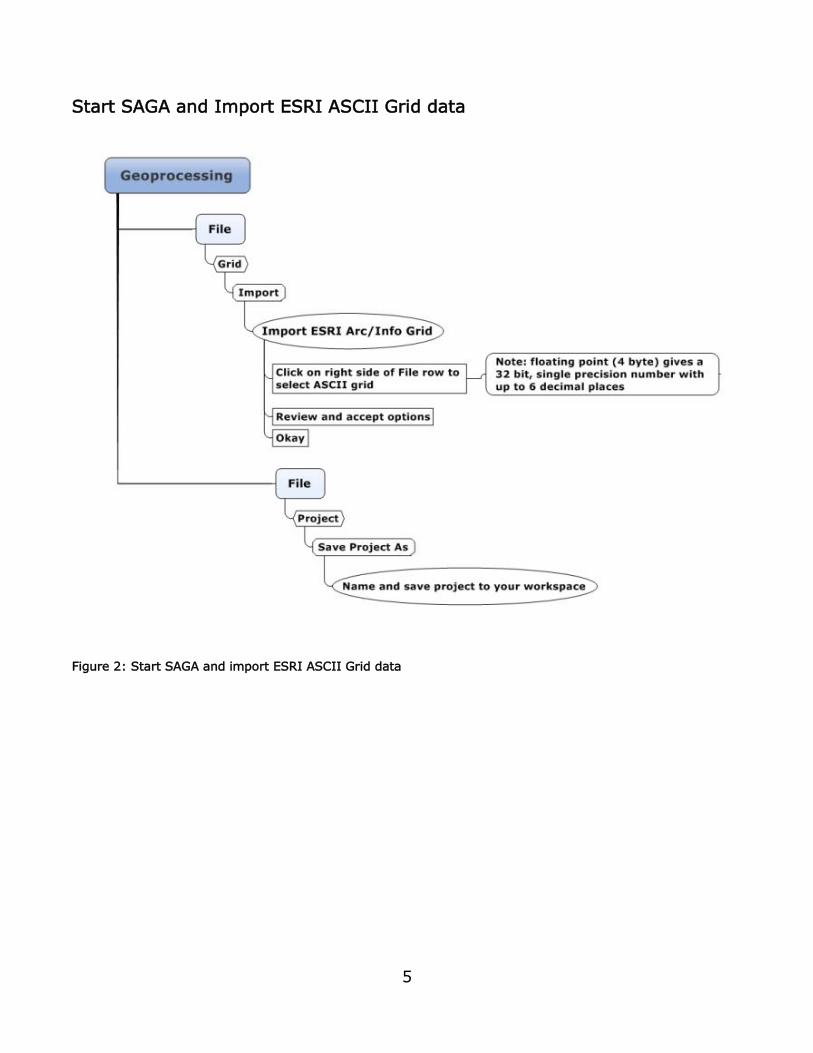
Start SAGA and Import ESRI ASCII Grid data
Figure 2: Start SAGA and import ESRI ASCII Grid data
6
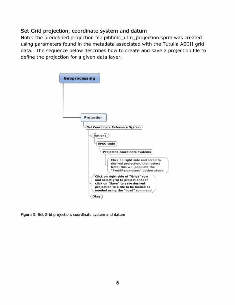
Set Grid projection, coordinate system and datum
Note: the predefined projection file pibhmc_utm_projection.sprm was created
using parameters found in the metadata associated with the Tutuila ASCII grid
data. The sequence below describes how to create and save a projection file to
define the projection for a given data layer.
Figure 3: Set Grid projection, coordinate system and datum

7
Export SAGA grid to ESRI ASCII grid format
Figure 4: Export SAGA grid to ESRI ASCII grid format

8
TERRAIN METRIC SEQUENCES

9
Slope, Aspect and Curvature
Calculates the local morphometric terrain parameters slope, aspect and if
supported by the chosen method also the curvature. Besides tangential curvature
also its horizontal and vertical components (i.e. plan and profile curvature) can be
calculated. (SAGA GIS Tool Description)
Figure 5: Slope, Aspect and Curvature

10
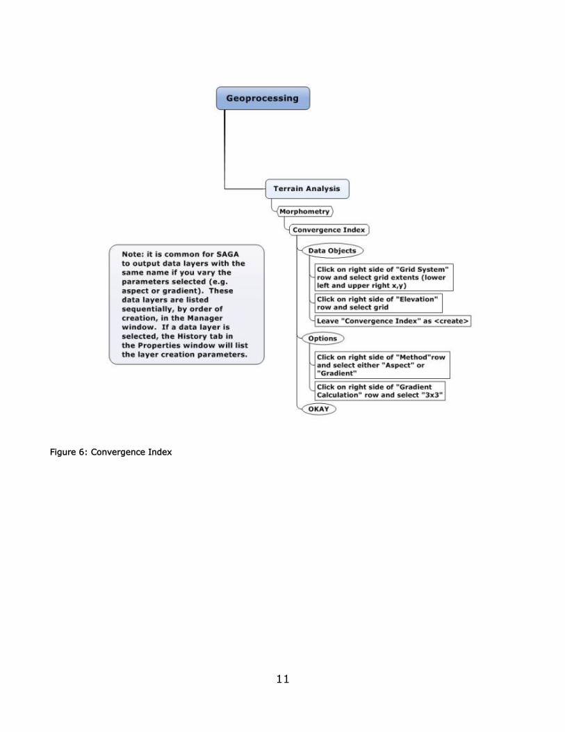
Convergence Index
Calculates an index of convergence/divergence [with] regard[ing] to overland flow.
By its meaning it is similar to plan or horizontal curvature, but gives much
smoother results. The calculation uses the aspects [or gradient] of surrounding
cells, i.e. it looks to which degree surrounding cells point to the center cell. The
result is given as [a] percentage[s], negative values correspond to convergent,
positive to divergent flow conditions. Minus 100 would be like a peak of a cone,
plus 100 a pit, and 0 an even slope.
(http://docs.qgis.org/2.6/en/docs/user_manual/processing_algs/saga/terrain_anal
ysis_morphometry/convergenceindex.html)
Convergence index is useful for analysis of lineaments especially represented by
ridges or channel systems as well as valley recognition tool
(https://svn.osgeo.org/grass/grass-
addons/grass7/raster/r.convergence/r.convergence.html)
Suggested approach: There are two choices for convergence index. The version
described here uses a window or filter – either 2x2 or 3x3 cells. For the way that
Kelvin is analyzing the results, a 3x3 window is appropriate. There is also a version
that uses a search radius, and allows for weighting, such as IDW, e.g. the farther
a cell is away from the center, the less influence it has with re: to convergence or
divergence. Gradient is the best “default” option, where just slope angle is the
driver. Aspect might be useful if there were some sort of landscape scale
directional trend (e.g. a dip or sloping trend in one direction). Gradient refers to
steepness of slope; aspect is cardinal direction that the slope faces.
11
Figure 6: Convergence Index

12
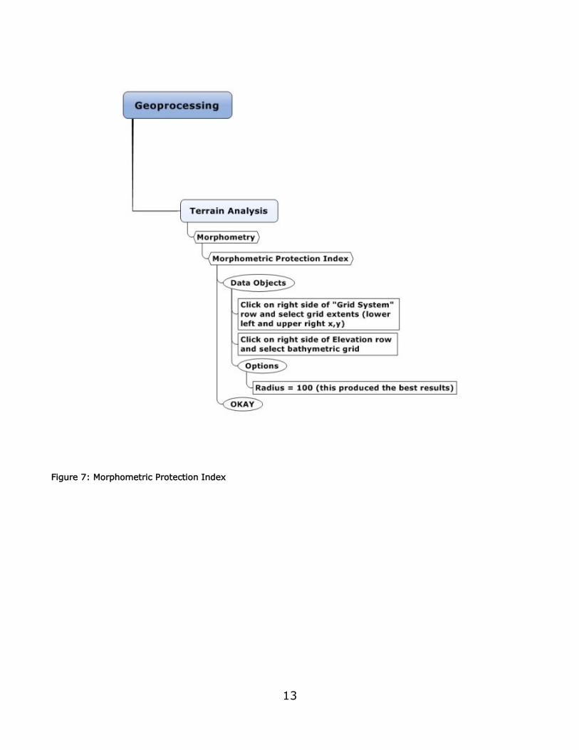
Morphometric Protection Index
SAGA output for this module is “Protection Index”.
This algorithm analyses the immediate surroundings of each cell up to a given
distance and evaluates how the relief protects it. It is equivalent to the positive
openness described in Yokoyama, R., et al. (2002).
Openness is an angular measure of the relation between surface relief and
horizontal distance. It resembles digital images of shaded relief or slope angle,
but emphasizes dominant surface concavities and convexities. Openness has two
viewer perspectives. Positive values, expressing openness above the surface, are
high for convex forms, whereas negative values describe this attribute below the
surface and are high for concave forms (Yokoyama, R., et al., 2002).
The value for any given cell is a function of a summary of surrounding cell values
in 8 directions. This is a relative metric, providing a positive or negative index
value based on the values of the surrounding cells.
The index is a mean value, so those cells with no data are (or at least should be)
accounted for by dividing the sum value by eight, even though there might only be
data for 5 cells… this is not explicit, but is the proper calculation method.
The unit for the “radius” option is the native cell size, in this case equivalent to
5m. One hundred is the default value, and was used for the initial example data,
not necessarily the optimal radius. The radius should be 15m for the first iteration
of Kelvin’s analysis, to match the 30m diameter cylinder around the sample point.
A detailed discussion of typical results from, and limitations of this metric are
presented in Appendix 2.
13
Figure 7: Morphometric Protection Index

14
Real Surface Area
Calculates real (not projected) cell area. (SAGA GIS). This is akin to rugosity, in
that it takes into account texture (i.e. the “ups and downs” within each cell) as
well as cell size. As the value increases, surface texture, or roughness, increases
(Grohmann, C.h., et al., 2009). The actual algorithm for calculation in SAGA is not
documented.
Figure 8: Real Surface Area
15
.
Terrain Ruggedness Index (TRI)
Riley et al. (1999) describe this as an objective quantitative measure of
topographic heterogeneity… by calculating the sum change in elevation between a
grid cell and its eight neighbor grid cells. This tool works with absolute values by
squaring the differences between the target and neighbor cells, then taking the
square root. Concave and convex shape areas could have similar values.
The output from this tool can be grouped / classified in whatever scheme the user
desires. That is the reason ESRI ASCII grids were generated, so that you could
use what you are familiar with to see which patterns pop out. You’ll also note that
the most “rugged” terrain is found in the Ikonos data – this is questionable data,
with a high degree of variance in cell values…
Options:
The radius of the moving window/filter can be set by the user, and that number
will determine how many cells are used to calculate the change in elevation. For
example, if the radius is set to 2, then 16 neighbor cells will be used in the
calculation. The radius distance is equal to the sum of the number of cells specified
(i.e. if the value is 2 and the cells are 5m, then the radius = 10m in actual
distance)
Weighting Function: 4 parameters available (no distance weighting, inverse
distance to a power, exponential, Gaussian weighting)
No weighting parameters were used in generating the example data set.
Finally, it should be noted that the value of this metric will vary as a function of
the size and complexity of the terrain used in the analysis.

16
Figure 9: Terrain Ruggedness Index (TRI)

17
Terrain Surface Convexity
Terrain surface convexity as proposed by Iwahashi and Pike (2007) for subsequent
terrain classification (SAGA GIS).
Convexity has been described as positive surface curvature…yielding positive
values in convex-upward areas, negative values in concave areas, and zero on
planar slopes. Each grid cell value represents the percentage of convex-upward
cells within a constant radius of ten cells (Iwahashi and Pike, 2007. pp.413-414).
Each cell is compared to all other cells within the constant radius window.
It should be noted that this metric is similar in nature to the Convergence and
Morphometric Protection indices. The differences lie in the method used for
calculation. Also, the percentage calculated is based on the number of cells within
the specified radius (10 for the sample data), and may not necessarily sum to 100.

18
Figure 10: Terrain Surface Convexity

19
Terrain Surface Texture
Terrain surface texture as proposed by Iwahashi and Pike (2007) for subsequent
terrain classification (SAGA GIS).
This parameter emphasizes fine versus coarse expression of topographic spacing,
or “grain”... Texture is calculated by extracting grid cells (here, informally, “pits”
and “peaks”) that outline the distribution of valleys and ridges. It is defined by
both relief (feature frequency) and spacing in the horizontal. Each grid cell value
represents the relative frequency (in percent) of the number of pits and peaks
within a radius of ten cells (Iwahashi and Pike, 2007. pp.412-413).
It should be noted that it is not clear that the relative frequency is actually a
percentage. According to Iwahashi and Pike (2007, p.30), To ensure statistically
robust classes, thresholds for subdividing the images are arbitrarily set at mean
values of frequency distributions of the input variables.

20
Figure 11: Terrain Surface Texture

21
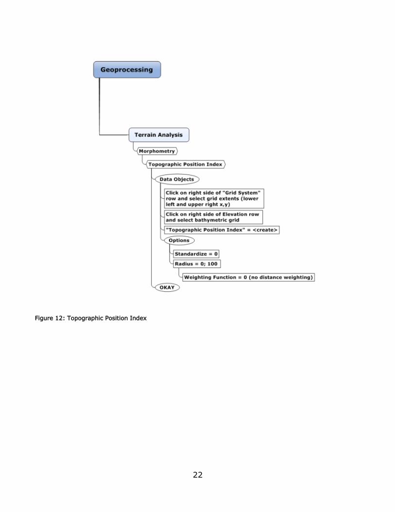
Topographic Position Index
Topographic Position Index (TPI) calculation as proposed by Guisan et al. (1999).
This is literally the same as the difference to the mean calculation (residual
analysis) proposed by Wilson and Gallant (2000). The bandwidth parameter for
distance weighting is given as percentage of the (outer) radius.
Weiss (2000) provides a very good description of the topographic position index
(TPI), and methods to derive a landscape classification from these values. The TPI
algorithm compares a DEM cell value to the mean value of its neighbors. The
mean value is calculated based on the shape selected by the user. Positive values
represent features typically higher than surrounding features, negative values
represent lower features, and values near zero are either flat or areas of constant
slope.
22
Figure 12: Topographic Position Index

23
TERRAIN CLASSIFICATION SEQUENCES
Note: the representations of terrain classifications provided as a supplement to
this report take one of several possible forms. They are primarily continuous, but
the user can create numeric or (e.g. 1.5 – 1.9) or categorical schemes (e.g. slope,
ridge) by thresholding the continuous or discrete landscape values.
24
Fuzzy Landform Element Classification
Algorithm for derivation of form elements according to slope, maximum curvature,
minimum curvature, profile curvature, tangential curvature, based on a linear
semantic import model for slope and curvature and a fuzzy classification Based on
the AML script 'felementf' by Jochen Schmidt, Landcare Research (SAGA GIS Tool
Description).
In simpler terms, this module uses slope, aspect and four measures of slope
curvature (minimum, maximum, plan and tangential) as inputs to an unsupervised
classification method (e.g. ISODATA, or k-means) to categorize terrain into natural
landform groupings (Irvin, et al., 1997; Petry, F., et al., eds., 2010). It also
calculates the relative uncertainty in the classification by describing how well a
specific grid cell and its associated terrain features fit within a given terrain class.
This is represented by the Maximum Membership, Entropy and Confusion Index
data layers and values.
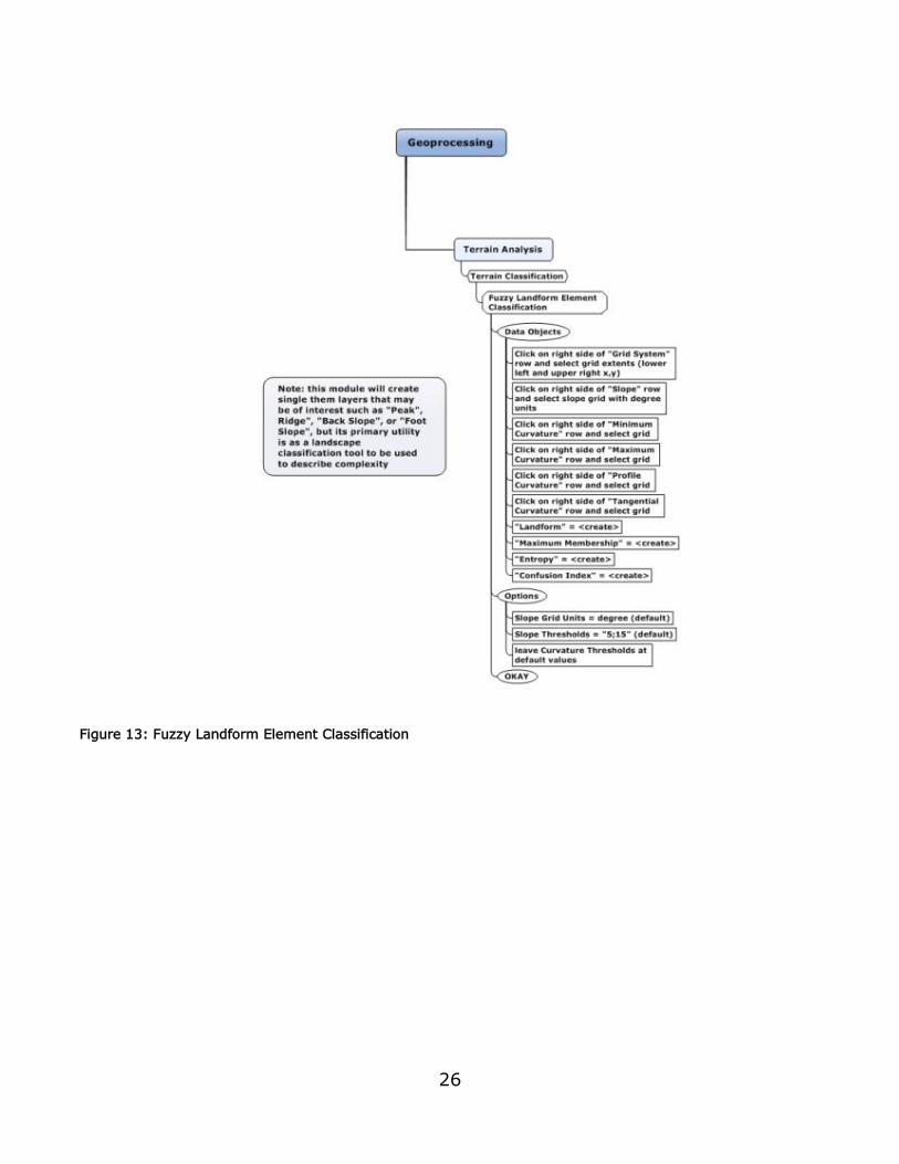
Note: this module requires Slope, Minimum, Maximum, Profile and Tangential
curvature grids as inputs. Irvin et al., 1997, describe these as “five principal
attributes” commonly used to describe landforms.
Options
Slope Grid Units: degree (default)
Slope Threshold: 5:15 (default)
It should be noted that this means the planar area is less than 5 degrees
(probslope=0) and slope area (probslope=1) is more than 15 degrees, and values
in between for this case yield a fraction between 0 and 1. For example, if the
terrain slope = 7, then the probability of classification as “flat” is 0.8, and
probability of classification as a slope is 0.2
Curvature Thresholds: 0.000002; 0.00005 (default)
It should be noted that these threshold values are labeled as “null” values,
indicating a lack of curvature, i.e. flat or planar terrain. These thresholds are then
used to calculate the probability that any given value falls within the vertical and
horizontal curvature value ranges for the various classes of curvature (e.g.
minimum, profile, etc.). The math is simple enough; the drivers are more the
curvature characteristics of the terrain being studied. These thresholds will vary
based on the type of terrain being characterized, and appropriate values for
“coral-based” terrain need to be determined.

25
Default Classes:
Function of slope, maximum curvature, and minimum curvature
Plain (Classification Value = 100), Pit (Classification Value = 111), Peak
(Classification Value = 122), Ridge (Classification Value = 120), Channel
(Classification Value = 101), Saddle (Classification Value =121)
Function of slope, profile curvature, tangent curvature
Back Slope (Classification Value = 0), Foot Slope (Classification Value = 10),
Shoulder Slope (Classification Value = 20), Hollow (Classification Value =1), Foot
Hollow (Classification Value = 11), Shoulder Hollow (Classification Value = 21),
Spur (Classification Value = 2), Foot Spur (Classification Value = 12), Shoulder
Spur (Classification Value = 22)
26
Figure 13: Fuzzy Landform Element Classification
27
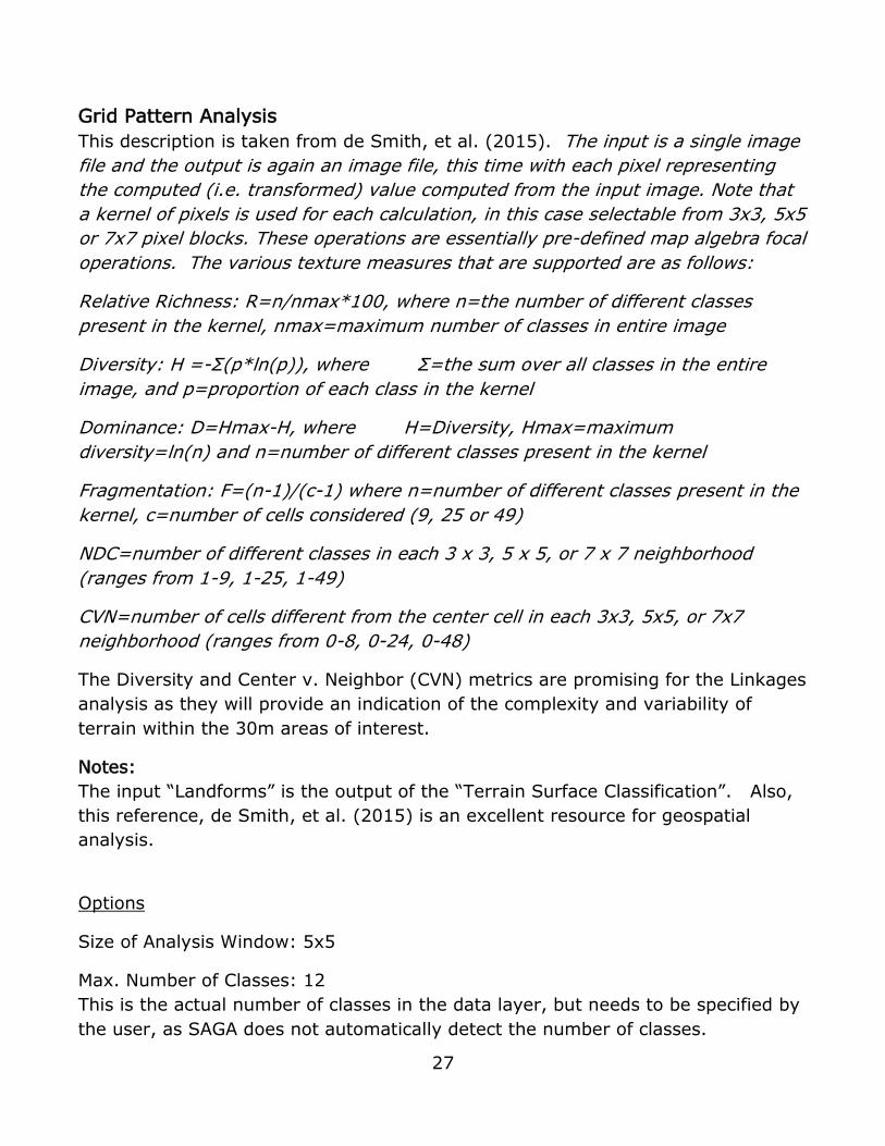
Grid Pattern Analysis
This description is taken from de Smith, et al. (2015). The input is a single image
file and the output is again an image file, this time with each pixel representing
the computed (i.e. transformed) value computed from the input image. Note that
a kernel of pixels is used for each calculation, in this case selectable from 3x3, 5x5
or 7x7 pixel blocks. These operations are essentially pre-defined map algebra focal
operations. The various texture measures that are supported are as follows:
Relative Richness: R=n/nmax*100, where n=the number of different classes
present in the kernel, nmax=maximum number of classes in entire image
Diversity: H =-Σ(p*ln(p)), where Σ=the sum over all classes in the entire
image, and p=proportion of each class in the kernel
Dominance: D=Hmax-H, where H=Diversity, Hmax=maximum
diversity=ln(n) and n=number of different classes present in the kernel
Fragmentation: F=(n-1)/(c-1) where n=number of different classes present in the
kernel, c=number of cells considered (9, 25 or 49)
NDC=number of different classes in each 3 x 3, 5 x 5, or 7 x 7 neighborhood
(ranges from 1-9, 1-25, 1-49)
CVN=number of cells different from the center cell in each 3x3, 5x5, or 7x7
neighborhood (ranges from 0-8, 0-24, 0-48)
The Diversity and Center v. Neighbor (CVN) metrics are promising for the Linkages
analysis as they will provide an indication of the complexity and variability of
terrain within the 30m areas of interest.
Notes:
The input “Landforms” is the output of the “Terrain Surface Classification”. Also,
this reference, de Smith, et al. (2015) is an excellent resource for geospatial
analysis.
Options
Size of Analysis Window: 5x5
Max. Number of Classes: 12
This is the actual number of classes in the data layer, but needs to be specified by
the user, as SAGA does not automatically detect the number of classes.
28
Figure 14: Grid Pattern Analysis

29
Surface Specific Points
Peuker and Douglas (1975) are cited as the reference to describe how this module
works. Unfortunately, this is a very difficult publication to obtain. These are
considered the “high information” points, and can be captured by interpolation
according to the following: An effective strategy is to start at the low point on a
stream or ridge, and to continue up until the high point is reached. Saddle points,
summits, and pits (depressions) are then places where the stream and ridge lines
converge. Algorithms exist to detect these features in grids, and to vectorize the
features for use in GIS[s] (Clarke, 1995, p.257).
The SAGA output is named “Result”, and grid cell values are determined by height
and slope of adjacent terrain cells. The possible range of values is -1 (negative) to
+1 (positive).
Figure 15: Surface Specific Points

30
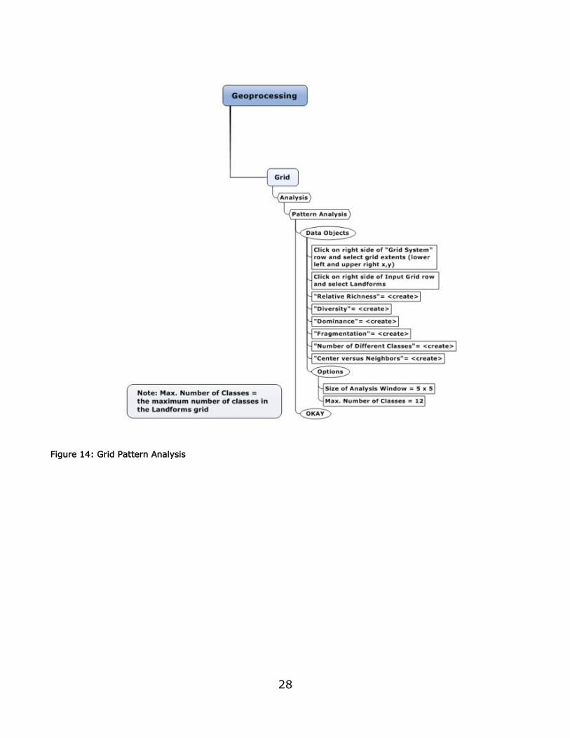
Terrain Surface Classification
Terrain surface classification as proposed by Iwahashi & Pike (2007). This module
derives a classification of the landscape based on slope, convexity and texture. Not
surprisingly, required inputs are: Slope, Convexity and Texture. The output grid is
Landforms. The user can select a classification based on 8, 12 or 16 landscape
categories.
It should be noted that this classification scheme is based on relative metrics, so
while a coarse scale analysis with lots of variation may yield a more dramatic
classification, at the island scale this tool may still yield something useful. All of
these metrics and classifications require user review and input to extract a useful
and representative classification scheme.
Slope is the first measure to be used in the classification, followed by Convexity
and Texture.
31
Figure 16: Terrain Surface Classification
32
TPI Based Landform Classification
Topographic Position Index (TPI) calculation as proposed by Guisan et al. (1999).
This is literally the same as the difference to the mean calculation (residual
analysis) proposed by Wilson and Gallant (2000). The bandwidth parameter for
distance weighting is given as percentage of the (outer) radius.
Weiss (2000) provides a very good description of the topographic position index
(TPI), and methods to derive a landscape classification from these values. The TPI
algorithm compares a DEM cell value to the mean value of its neighbors. The
mean value is calculated based on the shape selected by the user. Positive values
represent features typically higher than surrounding features, negative values
represent lower features, and values near zero are either flat or areas of constant
slope.
Ranges of TPI values can be used to generate a terrain classification or
categorization of features and landforms within a landscape. The sequence below
derives one such landscape classification. It is important to remember that the
TPI is scale dependent; meaning the size and shape of the focal area chosen to
calculate the initial values may highlight or ignore important landscape features.
In addition, the output is numeric only, so if desired, the user will need to assign a
categorical classification (e.g. backslope, foreslope, etc.)
Options
Radius = 0; 100
Radius = 0; 100
The first radius is the overall radius of the moving window. The second radius
allows for a continuous focal window (like a circle) or something different (like a
donut). See figure 2a in Weiss (2000).
Class Description Breakpoints 1 ridge > + 1 STDEV
2 upper slope > 0.5 STDV =< 1 STDV 3 middle slope> -0.5 STDV, < 0.5 STDV, slope > 5 deg 4 flats slope >= -0.5 STDV, =< 0.5 STDV , slope <= 5 deg
5 lower slopes >= -1.0 STDEV, < 0.5 STDV 6 valleys < -1.0 STDV
Weiss (2000) provides an example of a class definition scheme. It is unclear if this
scheme has been adopted and implemented in SAGA. In any case, categories and
thresholds are terrain-dependent and should be defined based on user needs.

33
Figure 17: TPI Based Landform Classification
34
References
Böhner, J., and Selige, T., 2006, Spatial prediction of soil attributes using terrain
analysis and climate regionalization, Göttinger Geographische Abhandlungen
v.115, pp.13-28
Clarke, K., 1995, Analytical and Computer Cartography, 2nd Edition, Prentice Hall,
New York. 290pp.
Dietrich, H., and Böhner, J., 2008, Cold Air Production and Flow in a Low Mountain
Range in Hessia (Germany) LandscapeHamburger Beiträge zur Physischen
Geographie und Landschaftsökologie – v.19, pp.37-48
http://downloads.sourceforge.net/saga-gis/hbpl19_05.pdf
Dikau, R., 1988, Entwurf einer geomorphographisch-analytischen Systematik von
Reliefeinheiten, Heidelberger Geographische Bausteine, Heft 5
Grohmann, C.H., et al., 2009, Surface Roughness of Topography: A Multi-Scale
Analysis of Landform Elements in Midland Valley, Scotland, Proceedings of
Geomorphometry 2009. Zurich, Switzerland, 31 August - 2 September, pp.140-
148
Guisan, A., Weiss, S.B., and Weiss, A.D., 1999, GLM versus CCA spatial modeling
of plant species distribution, Plant Ecology, v.143 pp.107-122
Hengl, T. and R. Hannes, eds., 2009, Geomorphometry; Concepts, Software and
Applications, Elsevier, Amsterdam, The Netherlands. 796pp.
Hjerdt, et. al, 2004, A new topographic index to quantify downslope controls on
local drainage, Water Resources Research, v.40, pp.1-6
Irvin, et al., 1997, Fuzzy and isodata classification of landform elements from
digital terrain data in Pleasant Valley, Wisconsin, Geoderma, v.77, pp.137-154
Iwahashi, J. & Pike, R.J., 2007, Automated classifications of topography from
DEMs by an unsupervised nested-means algorithm and a three-part geometric
signature, Geomorphology, Vol. 86, pp.409–440
Petry, F., et al., eds., 2010, Fuzzy Modeling with Spatial Information for
Geographic Problems, Springer, N.Y. 336pp.
35
Peucker, T.K. and Douglas, D.H., 1975, Detection of surface-specific points by
local parallel processing of discrete terrain elevation data, Computer Graphics and
Image Processing, 4, pp.375-387
Riley, S.J., et al. (1999), A Terrain Ruggedness Index That Quantifies Topographic
Heterogeneity, Intermountain Journal of Science, Vol.5, No.1-4, pp.23-27
De Smith, M., et al. 2015,
http://www.spatialanalysisonline.com/HTML/index.html?landscape_metrics.htm
Accessed March 27, 2015
Yokoyama, R., et al., 2002, Visualizing Topography by Openness: A New
Application of Image Processing to Digital Elevation Models, Photogrammetric
Engineering and Remote Sensing (68), No. 3, pp.257-266
Weiss, A.D., 2000, Topographic Position and Landforms Analysis,
http://www.jennessent.com/downloads/tpi-poster-tnc_18x22.pdf, Accessed March
27, 2015
Wilson, J.P., and Gallant, J.C., eds., 2000, Terrain Analysis - Principles and
Applications, Wiley, New York. 479pp.
36
Appendix 1: Metrics and Terrain Classification Options
Reviewed but Not Selected
Landscape Metrics
Curvature Classification – the only available documentation is in German. See
Dikau, R. (1988)
Diurnal Anisotropic Heating - not a structural metric - addresses diurnal heat
balance as influenced by topography… See Hengl, T. and R. Hannes, eds. (2009)
Downslope Distance Gradient – not a structural metric - this is a hydrologic
measure of the impact of local slope characteristics (e.g. convex or concave) on
the hydraulics gradient. See Hjerdt, et. al, (2004)
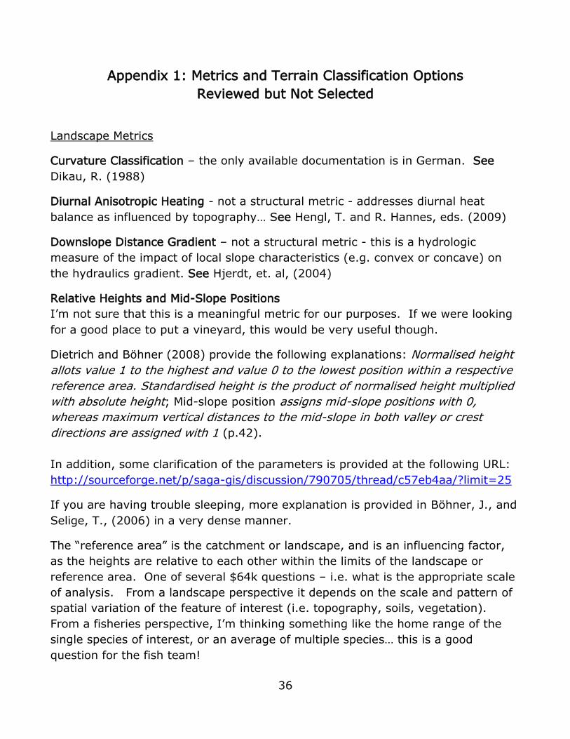
Relative Heights and Mid-Slope Positions
I’m not sure that this is a meaningful metric for our purposes. If we were looking
for a good place to put a vineyard, this would be very useful though.
Dietrich and Böhner (2008) provide the following explanations: Normalised height
allots value 1 to the highest and value 0 to the lowest position within a respective
reference area. Standardised height is the product of normalised height multiplied
with absolute height; Mid-slope position assigns mid-slope positions with 0,
whereas maximum vertical distances to the mid-slope in both valley or crest
directions are assigned with 1 (p.42).
In addition, some clarification of the parameters is provided at the following URL:
http://sourceforge.net/p/saga-gis/discussion/790705/thread/c57eb4aa/?limit=25
If you are having trouble sleeping, more explanation is provided in Böhner, J., and
Selige, T., (2006) in a very dense manner.
The “reference area” is the catchment or landscape, and is an influencing factor,
as the heights are relative to each other within the limits of the landscape or
reference area. One of several $64k questions – i.e. what is the appropriate scale
of analysis. From a landscape perspective it depends on the scale and pattern of
spatial variation of the feature of interest (i.e. topography, soils, vegetation).
From a fisheries perspective, I’m thinking something like the home range of the
single species of interest, or an average of multiple species… this is a good
question for the fish team!

37
I can try to (maybe) explain the parameters a bit more just for background:
“w” = the larger the catchment/reference area/landscape, the smaller the
influence is of any particularly high elevation
“e” = influences the position of any particular elevation by accounting for the
slope angle
“t” = determines the amount of influence the highest elevation value in a window
has on the relative height calculation
http://sourceforge.net/p/saga-gis/discussion/790705/thread/c57eb4aa/?limit=25
According to the forum URL above,
w: weights the influence of catchment size on relative elevation (inversely
proportional)
e: controls the position of relative height maxima as a function of inclination
t: controls the amount by which a max. in the neighborhood of a cell is taken over
into the cell (smaller the t, the smoother the result)
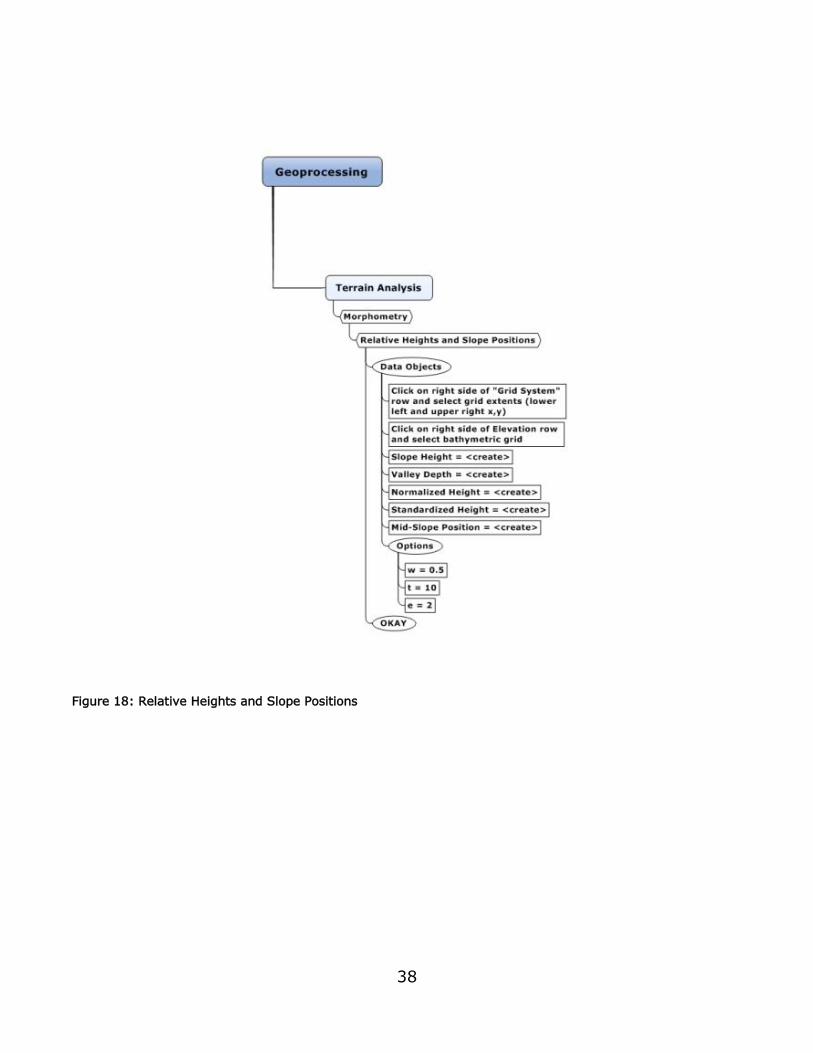
38
Figure 18: Relative Heights and Slope Positions

39
Terrain Classification
Fragmentation (Standard and Alternative), found under Grid => Analysis – this
module produces density (identifies interior and exterior/edge patches),
connectivity (indicates connectivity between patches) and fragmentation data
layers using the standard “moving window” approach. These layers are typical
outputs for a fragmentation analysis. The issue with the SAGA implementation is
that only a single class can be analyzed per iteration. Therefore with the Tutuila
pilot data, which is a 12-class data layer, this analysis would have to be run 12
separate times and them merged in some fashion and interpolated. This is not a
scientifically sound or feasible approach.
Patch Analyst – this is an implementation of the Fragstats software within the
ArcGIS environment. Modules that operate on polygons and grids are available.
Classification data layers can be analyzed at the landscape and patch scale. The
“Landforms” layer, created using the procedure outlined under Terrain Surface
Classification (p.25 of this document) was reclassed using the “Name” attribute, to
“Class_1” through “Class_12”. Class number increased as the default value
ranges increased. It should be noted that the reclassification could be more
meaningful if expert knowledge were applied to interpolate the classification. This
data layer was then exported to the ESRI ASCII Grid format, imported to ArcGIS
as a raster grid, then converted to polygons. The “Spatial Statistics” option under
“Patch Analyst” was used to generate both landscape and patch scale metrics.
Outputs are both tabular and thematic, with the majority of the output contained
in the table, where one value characterizes the landscape or the universe of
classes (e.g. Patch Density & Size Metrics, Edge Metrics, Shape Metrics,
Diversity Metrics). Thematic outputs are a data layer with Mean Shape Index,
Mean Perimeter-Area Ratio, and Mean Patch Fractal Dimension attributes
associated with each polygon.
For the Linkages analysis, a single index value describing landscape or patch
assemblage characteristics has very little value, unless perhaps an island scale
analysis is undertaken (e.g. total fish biomass for a island A, related to the entire
landscape metric , compared to the same variables for island B). In addition, it is
not clear what value the thematic metrics might have with regard to fish
demographics.

40
Appendix 2: Evaluation of “No Data” areas and Morphometric
Protection Index
Figure 19: a) SAGA-generated “No data” area; b) bathymetry “No data” area
This is a comparison of no data areas in the original input bathy file (b) and the
morphometric protection index with a 100 cell radius (a). The width of the “no
data” area in the original is approximately 95 cells at its widest point, while the
protection index is approximately 275 cells.
Measurements were not exact, but show general agreement, i.e. taken from the
center pixel of the input the output should be approximately 286 cells in width
(95/2 = 42.5 (43); 43 + 100 = 143; 143 *2 = 286).
a
b
41
Figure 20: a) SAGA-generated artifacts; b) bathymetry “No data” areas
This graphic illustrates the original bathy with small “no data” gaps and the MPI
output with odd star-shaped patterns. It is reasonable to expect this to be a no
data blob with a 100 cell radius. Instead we have a star with 100 cell legs… The
layer created using a 200 cell radius (not shown here) displays the same
relationships.
However, in Yokoyama, et al., 2002, the angular change in elevation is calculated
in a similar pattern to what we are seeing. I have to confess that while I
a
b

42
understand the concept, I don’t completely understand the implementation… What
we are seeing is what I would call an “artifact”. Sometimes this raster processing
business generates odd results.
As you are looking at the data, you are seeing issues of data quality that are not
unexpected. Based on this result alone, I would recommend that you take the
original merged multibeam/Ikonos bathy grid and run a majority filter over it to fill
in no data gaps such as those shown above. The decision rule for you is how big
to make the majority window. For example, the two rectangles shown in the
image above are 5 x 10 cell data gaps.


![[REDACTED] FINAL 2009 BATHYMETRIC SURVEY OF PILOT ...](https://static.fdocuments.us/doc/165x107/61ca8c4f0953c566e845b7a5/redacted-final-2009-bathymetric-survey-of-pilot-.jpg)


