Uppsala Master’s Thesis inComputing Science 139Examensarbete TF31998-12-08ISSN 1100-1836

Terrain Analysis with Radio Link Calculations for aMap Presentation Program

Oskar Wibling

Computing Science DepartmentUppsala University

Box 311S-751 05 Uppsala

Sweden

This work has been carried out atSjöland & Thyselius AB

Sehlstedtsgatan 6115 28 Stockholm

Sweden

Abstract

A plugin module for terrain analysis including radio link calculations hasbeen constructed for a map presentation program (currently referred to asUniMap). The module contains tools for radio link calculations, terraininformation, target sight, free sight boundary and sight field. It isimplemented as a DLL using the COM programming model. All of theprogramming was done in C++ using the MFC (Microsoft FoundationClasses) library and Microsoft Visual Studio (Visual C++) as programmingenvironment. GeoPres API was used for most of the geographicalpresentation. The main focus of the work was to review radio link calculationmethods and to implement a few of those in the module. The goal was to beable to make more exact calculations than the ones that can be made inanother map presentation program called MilMap (that also has beendeveloped by Sjöland & Thyselius AB). As a consequence most of the reportis about radio transmission loss calculation techniques and wave propagationphenomena. Some well known methods for calculating the attenuation whenmodeling the radio link environment in different ways are described. Acomparison has also been made between the prediction accuracy in the radiolink calculation methods that were implemented in the UniMap module andthe methods in MilMap. Even though the amount of available measurementdata was not sufficient to draw any statistically valid conclusions thecomparisons indicate that it is probable that an improvement has been made.

Supervisor: Richard Mohringe, Sjöland & Thyselius ABExaminer: Faron Moller, Computing Science Department, Uppsala University

Passed:

Oskar Wibling ii

UPTEC F 98 101 Master´s degree project

DEC 1998

Terrain Analysis with Radio LinkCalculations for a Map PresentationProgram

OSKAR WIBLING

Oskar Wibling iii

Engineering Physics ProgrammeUppsala University School of Engineering

UPTEC F 98 101 Date of issue981208

AuthorWibling Oskar

Title (English)Terrain Analysis with Radio Link Calculations for a Map Presentation Program

Title (Swedish)-

AbstractA plugin module for terrain analysis including radio link calculations has been constructed for a mappresentation program (currently referred to as UniMap). The module contains tools for radio link calculations,terrain information, target sight, free sight boundary and sight field. It is implemented as a DLL using the COMprogramming model. All of the programming was done in C++ using the MFC (Microsoft Foundation Classes)library and Microsoft Visual Studio (Visual C++) as programming environment. GeoPres API was used for mostof the geographical presentation. The main focus of the work was to review radio link calculation methods and toimplement a few of those in the module. The goal was to be able to make more exact calculations than the onesthat can be made in another map presentation program called MilMap (that also has been developed by Sjöland& Thyselius AB). As a consequence most of the report is about radio transmission loss calculation techniquesand wave propagation phenomena. Some well known methods for calculating the attenuation when modeling theradio link environment in different ways are described. A comparison has also been made between the predictionaccuracy in the radio link calculation methods that were implemented in the UniMap module and the methods inMilMap. Even though the amount of available measurement data was not sufficient to draw any statisticallyvalid conclusions the comparisons indicate that it is probable that an improvement has been made.

KeywordsRadio link, wave propagation, transmission loss, terrain analysis, C++, Microsoft Windows, MFC, DLL, COM,GeoPres, MapObjects

Supervisor(s)Richard Mohringe, Sjöland & Thyselius AB

ExaminerFaron Moller, Computing Science Department, Uppsala University

Project nameUniMap

SponsorsSjöland & Thyselius AB

LanguageEnglish (with an appendix in Swedish)

Security-

ISSN 1401-5757Pages65

Supplementary bibliographical informationSjöland & Thyselius AB report 98:02.OW

School of Engineering, Studies Office Phone: +46-(0)18-4713003Visiting address: Lägerhyddsvägen 2, bldg 4, Uppsala Fax: +46-(0)18-4713000Postal address: Box 823, SE-751 08, Uppsala, Sweden E-mail: kansli@uth.uu.se

Oskar Wibling iv

Contents

Contents...................................................................................................................iv

1 Introduction.........................................................................................................1

2 Radio wave propagation theory ..........................................................................12.1 The radio wave ..................................................................................................................... 12.2 The radio system .................................................................................................................. 22.3 The transmission channel...................................................................................................... 32.4 The Fresnel-zone ellipsoids................................................................................................... 42.5 The theorem of reciprocity.................................................................................................... 52.6 The effect of the troposphere................................................................................................. 52.7 Multipath propagation .......................................................................................................... 62.8 Simplified models of the terrain ............................................................................................ 7

2.8.1 Modeling with a smooth, spherical earth .................................................................... 72.8.2 Modeling with knife-edges......................................................................................... 82.8.3 Modeling with a dielectric slab................................................................................... 82.8.4 Modeling with cylindrical shapes ............................................................................... 82.8.5 Using an empirical clutter factor................................................................................. 9

3 Attenuation calculation methods ........................................................................9

3.1 Free space attenuation model ................................................................................................ 93.2 Smooth spherical earth attenuation models ...........................................................................12

3.2.1 The two-wave model.................................................................................................133.2.2 A model that also accounts for the surface wave ........................................................143.2.3 Accounting for the curvature of the earth...................................................................16

3.3 Single knife-edge diffraction attenuation model....................................................................173.4 Simplified multiple knife-edge diffraction methods ..............................................................20

3.4.1 Bullington’s method..................................................................................................203.4.2 The Epstein-Peterson method....................................................................................213.4.3 The Deygout method.................................................................................................213.4.4 The Giovaneli method...............................................................................................223.4.5 Other simplified models ............................................................................................23

3.5 The Vogler knife-edge diffraction method............................................................................243.5.1 The calculation method.............................................................................................243.5.2 Example calculations ................................................................................................28

3.6 Selecting the heights for diffraction attenuation calculations.................................................293.6.1 The Fresnel zone approach........................................................................................303.6.2 The elevation method................................................................................................30

3.7 Vegetation attenuation models .............................................................................................313.8 Built up area attenuation model............................................................................................323.9 Atmospheric attenuation models ..........................................................................................333.10 Total path loss calculation methods......................................................................................35

3.10.1 The Blomquist and Ladell methods ...........................................................................353.10.2 The JRC method .......................................................................................................363.10.3 Geometrical theory of diffraction ..............................................................................363.10.4 Statistical methods ....................................................................................................37

4 The Microsoft Foundation Class Library.........................................................37

5 DLLs and COM.................................................................................................37

5.1 Dynamic link libraries .........................................................................................................375.2 The Component Object Model .............................................................................................38

5.2.1 IUnknown.................................................................................................................385.2.2 Class factories...........................................................................................................38

Oskar Wibling v

5.2.3 Registration of COM classes .....................................................................................39

6 Digital maps .......................................................................................................39

7 MapObjects and GeoPres..................................................................................40

7.1 MapObjects .........................................................................................................................407.2 The GeoPres API.................................................................................................................40

8 The radio link calculations in MilMap .............................................................40

9 The new terrain analysis module ......................................................................41

9.1 Structure of the databases used.............................................................................................419.2 The radio link calculation method in the module ..................................................................429.3 The terrain information tool in the module ...........................................................................449.4 The target sight calculation method in the module ................................................................449.5 The free sight boundary calculation method in the module....................................................449.6 The sight field calculation method in the module..................................................................44

10 Evaluation and discussion .................................................................................44

10.1 Testing the new radio link calculation method......................................................................4410.2 Error sources in the radio link tool .......................................................................................4610.3 The other new terrain analysis tools .....................................................................................46

11 Future work .......................................................................................................46

12 Acknowledgements ............................................................................................47

13 References..........................................................................................................47

Appendix ................................................................................................................51

A Relative permittivity and conductivity constants .............................................51

B User’s manual for the developed system (in Swedish)......................................51

B.1 Uppstart av systemet.....................................................................................51

B.2 De olika verktygen som ingår .......................................................................52

B.2.1 Radiolänkverktyget ...................................................................................................52B.2.2 Terränginformationsverktyget ...................................................................................53B.2.3 Målsiktverktyget .......................................................................................................53B.2.4 Frisiktsgränsverktyget ...............................................................................................54B.2.5 Siktfältverktyget .......................................................................................................54

B.3 Inställningar..................................................................................................55

B.3.1 Inställningar i radiolänkverktyget ..............................................................................55B.3.2 Övriga inställningar ..................................................................................................58

B.3.2.1 Inställningar för terränginfoverktyget...........................................................58B.3.2.2 Inställningar för målsiktverktyget.................................................................58B.3.2.3 Inställningar för frisiktsgränsverktyget .........................................................59B.3.2.4 Inställningar för siktfältverktyget .................................................................59B.3.2.5 Terrängtyper för siktberäkningar..................................................................60

Oskar Wibling 1

1 Introduction

A plugin module for terrain analysis including radio link calculations has been constructed for a mappresentation program that in this text sometimes will be referred to as UniMap. The module containstools for radio link calculations, terrain information, target sight, free sight boundary and sight field. Itis implemented as a DLL using the COM programming model. Hence, the terrain analysis module is aCOM-object that is used by the main application.

• The radio link tool contains a number of numerical methods for calculating the attenuation of aradio signal between two radio stations that have been positioned on the map.

• When the terrain information tool is active information about the altitude of the ground (with orwithout the height of the terrain dress included) and terrain type are printed in the status bar whenthe mouse pointer is positioned on the map.

• The target sight tool lets the user position an observation point and a target point on the map andindicates by coloring a line between these points red or green if there is free sight or not.

• The free sight boundary tool lets the user position an observer on the map and then searches thedistance to the first point where the line of sight to a target is obscured. A connecting boundarybetween the points that have been calculated for a number of angles is then drawn onto the map.

• The sight field tool searches a number of target positions around an observer and indicates withpoints if the line of sight between observer and target is unobstructed.

The main difference between the free sight boundary tool and the sight field tool is that the formerstops at the first target positions that are obstructed from the observer. The sight field tool can searchboth inside and outside of this limit but does not connect the found points with a line.

For a more detailed description, with illustrations, of how the system looks the reader is referred toAppendix B where the users manual (in Swedish) is enclosed.

Since it was requested that the tools would look as similar as possible to a module in another mappresentation program developed by Sjöland & Thyselius AB called MilMap a lot of inspiration wastaken from that program when developing the GUI (Graphical User Interface).

All of the programming was done in C++ using the MFC (Microsoft Foundation Classes) library.Microsoft Visual Studio (Visual C++) was used as programming environment. GeoPres API was usedfor most of the geographical presentation.

The main focus of the work has been to review radio link calculation methods and to find out whichones are suitable to implement in the module. Therefore most of the report is about radiocommunication calculation techniques. The theory behind the other tools are covered briefly in themain part of the report and also in the users manual (see Appendix B).

A comparison is also made between the new radio link calculation method and the method in MilMap.

2 Radio wave propagation theory

2.1 The radio wave

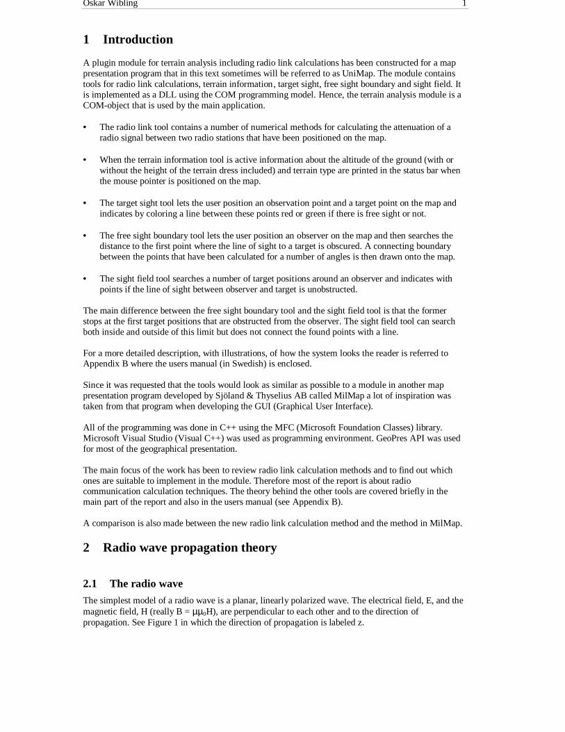
The simplest model of a radio wave is a planar, linearly polarized wave. The electrical field, E, and themagnetic field, H (really B = µµ0H), are perpendicular to each other and to the direction ofpropagation. See Figure 1 in which the direction of propagation is labeled z.

Oskar Wibling 2

Figure 1-A linearly polarized electromagnetic wave

That a wave is planar means that it has a plane wavefront, i.e. that the field at a certain moment has thesame phase in all the points of a plane that is perpendicular to the direction of propagation. In mostcases the assumption that the wavefront is planar is a very rough approximation. In most real lifesituations the wave is reflected by several obstacles in the surrounding terrain and the signal reachingthe receiver is coming in from a number of different directions.

A wave that is linearly polarized can be vertically or horizontally polarized. In vertical polarization theelectrical field is directed vertically and the magnetic field is directed horizontally. In horizontalpolarization the two fields are directed in the perpendicular directions from vertical polarization.

The polarization of the radio wave is affected when the wave is reflected. After several reflections thepolarization of the wave becomes nearly random. This effect is often neglected in calculations and thewave is assumed to have a certain polarization independent of the number of reflections. Thedepolarization effects can then instead be modeled by a change in amplitude of the reflected signal.

The propagation speed of an electromagnetic wave in vacuum is given by:

[m/s]c 1099792458.21 8

000 ⋅≈=

εµ

where µ0 [Vs/Am] is the permeability of free spaceε0 [As/Vm] is the permittivity of free space

The frequency of the wave is the number of completed revolutions per second and the wavelength invacuum is given by:

[m]f

c 0=λ

where f [s-1] is the frequency of the wave

2.2 The radio system

The assumption is made that the radio system that is used is a standard point-to-point connection with atransmitter and a receiver. This is the case in the type of radio link connections that are the focus of thiswork. The transmitter and the receiver each have a connecting cable and an antenna. Se Figure 2 for anillustration of this. In a radio link the antennas are usually elevated considerably (12 meters or more)

Oskar Wibling 3

above the ground and clear from vegetation and other obstacles in the direction towards the otherantenna. The frequency of the carrier wave in a radio link is usually in the lower microwave range.

Figure 2 – The radio system

Sometimes the frequency characteristics of the transmission cables used are available. The attenuationcaused by the cables at a certain frequency can then be interpolated from tabulated values. However, aconstant value is often given for the cable damping and is used at all frequencies.

The antenna gains may be recalculated for different frequencies and locations, but are often also givenas constant values.

2.3 The transmission channel

The signal that is transmitted between two radio stations is affected by the frequency characteristic ofthe transmission channel. If the characteristic of the channel is fairly even and undistorted within thefrequency region used the signal can be considered as narrow band when performing wave propagationcalculations. In effect this means that only the signal level at the center frequency (carrier wavefrequency) is of interest when judging the quality of the channel. Hence, only the attenuation of a sinewave with the center frequency is often considered when performing signal quality predictions. If thefrequency characteristic is very uneven it is not enough to know the attenuation of the center frequencyand more thorough calculations will have to be made.

The performance of the radio system is to a large extent dependent on the propagation situation. Theradio signal can be reflected, refracted and attenuated by terrain, buildings and the transmissionmedium (air, rain, fog etc.). To be able to make predictions about the quality of the signal, especially atpropagation near the surface of the earth, simplified models are usually employed. Different wavepropagation phenomena are treated separately and combined in a total model suitable for the situationat hand. Of course, the approximations that are made introduce significant prediction errors.

The simplest of all wave propagation models is the free space propagation model in which all obstaclesthat may affect the field are disregarded. The propagation of the wave is assumed to be in vacuum andno obstacles are obstructing the path. Even though the model is best for predicting for example satellitecommunication attenuation it does a good job in providing rough estimates of field strengths andreceived powers. The free space attenuation is only dependent on frequency and distance.

To maximize the power transaction the transmitting antenna should be built as to provide anelectromagnetic field that has the largest possible amplitude at the receiving antenna. The receivingantenna should be built as to utilize the given field optimally. Both of these are accomplished by givingthe antennas a suitable directivity. It is also important that both antennas are constructed for a suitablepolarization of the electromagnetic field (usually vertical or horizontal polarization).

When less simplified models are used a propagation factor can be defined as the ratio between theactual received power in a certain propagation situation and the corresponding received power for freespace propagation, at a certain distance from the transmitter. This is written as:

[dB]P

PF

fs

r log10 10

=

The total attenuation of the signal is therefore given by:

Oskar Wibling 4

[dB]FAA fstot +=

where Afs [dB] is the free space attenuationF [dB] is the propagation factor

This viewpoint simplifies the study of the attenuation the terrain causes since that effect is completelycontained in F and thus disconnected from the free space attenuation. The attenuation in excess to thefree space attenuation is thus often calculated separately and added to the free space attenuation. Fmight be a sum of several propagation factors.

2.4 The Fresnel-zone ellipsoidsIn Figure 3 the path between transmitter and receiver has been drawn with a plane normal to the pathsomewhere between the stations. The circles drawn on the plane symbolize a family of circles with thespecific property that the total path length from transmitter (T) to receiver (R) via each circle is nλ/2longer than the path T-O-R where n is an integer. Clearly, the radii of the individual circles depend onthe location of the imaginary plane with respect to the path terminals. The radii are largest midwaybetween the terminals and become smaller as the terminals are approached.

Figure 3 - Family of circles defining the limits of the Fresnel zones at a given point on the radiopropagation path

When the circles are drawn for all possible positions of the plane between the two stations a family ofellipsoids, called the Fresnel ellipsoids, are formed. The radius of any specific member of the familycan be expressed as:

21

21

dd

ddnrn +

= λ

Which is an approximation that is valid provided that d1>>rn and d2>>rn. This is realistic except in theimmediate vicinity of the terminals.

An alternative formulation of the equation for calculating the Fresnel radius that is often used inpractice is the following:

( ) ( ) [m]ddf

ddfddr 5.547,,

21

2121 +

=

where d1 and d2 are in kmf [MHz] is the frequency of the radio wave

The volume enclosed by the ellipsoid defined by n = 1 is known as the first Fresnel zone. The volumebetween the first Fresnel zone and the ellipsoid defined by n = 2 is the second Fresnel zone and so on.The Fresnel zones are interesting because if an obstructing screen was actually placed at a pointbetween the transmitter and receiver then if the radius of the aperture (i.e. the hole in the screen) was

Oskar Wibling 5

increased from that corresponding to the first Fresnel zone to that defining the limit of the secondFresnel zone, then to the third Fresnel zone etc. the field would oscillate. The amplitude of theoscillation would gradually decrease since smaller amounts of energy propagate via the outer zones.

In radio communication applications and especially when higher frequencies are used, it is alwaysdesirable to have a clear line of sight between the two radio stations. Additionally, it is also desirable tohave as many of the Fresnel zones as possible clear of obstacles. A demand that is often made on thelocations of antennas is that at least the first Fresnel zone is clear of obstacles.

In Figure 4 a radio path is drawn with the straight line between the stations and the first Fresnel zoneindicated. The distance between the stations is 17 km and the frequency used is 2.3 GHz. Note thatneither of the straight line between the stations, nor the first Fresnel zone is clear of obstacles in thiscase.

Figure 4 – A radio path with the first Fresnel zone shown

2.5 The theorem of reciprocity

An important result from the theory for linear, electrical systems is the theorem of reciprocity. It can beapplied in almost all investigations of propagation with the exception of ionospheric propagation. Aconsequence of the theorem is that the propagation attenuation stays unchanged if the transmitter isused as receiver and vice versa. This means that with a given set of antennas and antenna positions thesame propagation attenuation is received for both directions of transmission.

2.6 The effect of the troposphereTo account for the diversion of beams due to the presence of the troposphere an effective earth radiusthat is larger than the actual radius can be used. This assumption makes it possible to see theelectromagnetic waves as following straight lines instead of curved ones and greatly simplifies themodeling. See Figure 5 for an illustration of this. Another assumption that is often also made is that theearth is surrounded by air of constant index of refraction.

Figure 5 – The use of an effective earth radius

The effective earth radius, Re, can under the assumptions above be calculated according to thefollowing method [1].

Snellius equation for refraction in spherical surfaces is given by:

( ) ( ) (1) coscos 222111 θθ RnRn =

where n1, n2 are the refractive indices of the respective mediaR1, R2 are distances from the shared centerpoint to a point in the respective media

Oskar Wibling 6

θ1, θ2 are the grazing angles

The ITU-R has defined a special model for the normal atmosphere (a calm and idealized modelatmosphere). For small altitudes, the refractive modulus of the reference atmosphere may beapproximated according to:

( ) (2) 039.0315104

31510315101 6

0

66 hR

hKhnN −≈⋅−=⋅−=⋅−=

where n is the refractive indexK [km-1] is a constantR0 [km] is the radius of the earthh [m] is the altitude of the point

Using (1) and (2) then yields the following expressions for the two earth spheres.

Real earth: ( ) ( )( ) ( )100000 coscos θθ hRKhnRn +−=Model earth: ( ) ( ) ( )1000 coscos θθ hRnRn ee +=

where R0 [km] is the radius of the real earth (approximately 6370 km)Re [km] is the radius of the model earthn0 is the refractive index of the atmosphereθ0, θ1 are the grazing anglesh [m] is the altitude of the point

Dividing the two equations yields:

( ) 00

0

00

00

3

4

1R

KR

R

hRKn

RnRe ≈

−≈

+−≈

Thus, if a model earth with a radius of 4/3 times the real earth radius is used in all calculations therefraction phenomenon can be ignored and good results can still be achieved.

2.7 Multipath propagation

Multipath propagation is caused by reflections in terrain and buildings. The signal that reaches thereceiver is composed of several components that correspond to different propagation paths withdifferent attenuation and distance. Since the total wave is a vectorial sum of the components it islargely affected by the relations in phase between them. One extreme case is the one in which thecomponents totally cancel each other out. The other extreme case is where they cooperateconstructively to give an amplified signal. If a station is moving in the terrain the difference in timebetween the components can appear to be random and small changes in the antenna position canradically change the amplitude of the signal. This effect is often referred to as multipath fading but willnot be examined further here.

Usually most multipath propagation phenomena are neglected when estimating channel quality since itgreatly simplifies the calculations. If a two dimensional model of only the terrain between the two radiostations, a cross section or slice of the earth, is used most of these effects are disregarded. Se Figure 6for an illustration of this.

Oskar Wibling 7

Figure 6 – A 3D radio path and a simplified 2D model of the path

However, in recent years, efforts have been made to develop three dimensional wave propagationprediction models. See [38] for further information.

Since the two dimensional model of the propagation path is still too complex it is usually modeled withsimpler objects such as for example knife-edges.

2.8 Simplified models of the terrain

In radio signal attenuation calculations terrain differences are sometimes neglected completely and theearth modeled as a completely smooth sphere. However, if a more exact prediction of the totalattenuation is needed it is necessary to consider the diffraction effects caused by rough terrain obstaclessuch as hills and mountains. Waves with short wavelengths (i.e. high frequencies) are more attenuatedby these kinds of obstacles than waves with long wavelengths (i.e. low frequencies). The reason for thisis that diffraction allows radio signals to propagate around the curved surface of the earth and alsobehind obstacles. Since it would be infeasible to include every obstacle on the path in the calculationsthe terrain is usually modeled with simple geometrical shapes. A selection of these are knife-edges,dielectric slabs and cylindrical shapes. Alternatively, the terrain is not modeled at all, but instead itsinfluence is added as an empirical clutter factor to a theoretical basic approximation. A common way ofdoing this is to add excess clutter loss to the attenuation received when using a smooth, spherical earthmodel.

A model based method has two main sources of error:

(1) The description of the terrain is too simplified.(2) The calculation of the propagation over the terrain model is an approximation.

An empirical method also has two main sources of error:

(1) The effect a certain terrain formation has on the total attenuation cannot be separated in anunambiguous manner.

(2) The measurements that were used for constructing the model were made under certaincircumstances regarding environment, frequency range and antenna heights. The correctness whenlater using the method is largely dependent on that the circumstances are similar to the originalones.

2.8.1 Modeling with a smooth, spherical earthA very simple model of the terrain is that of a completely smooth, spherical earth. The model can beused at low frequencies and in regions with moderately uneven terrain with decent results. Over oceansthe model can also be used at higher frequencies.

Oskar Wibling 8

2.8.2 Modeling with knife-edgesOne commonly used shape is an infinitely thin, perfectly absorbing or conducting, knife-edge withlimited height but unlimited length. The electrical properties of the knife-edge are basically unessentialwhen the field behind the edge (in the shadow region) is the interesting one. The main obstacles on thepath between transmitter and receiver are selected using some method (see section 3.6) and arereplaced by knife-edges with the same heights above the sea as the original obstacles. See Figure 7 foran example of an original terrain profile and the profile approximated by a number of knife-edges.

Figure 7 – Terrain profile and knife-edge approximation of the profile

Knife-edges are often used when calculating the diffraction attenuation from obstacles on the pathbetween transmitter and receiver. The diffraction attenuation from obstacles in the terrain rises sharplywith frequency. At higher frequencies (from about 200 MHz) the propagation factor caused byobstacles on the path will almost always dominate over the propagation factor for an even, sphericalearth.

2.8.3 Modeling with a dielectric slabLayers covering the ground can be included in the model to block ray paths or add attenuation to apropagation path over or through the layer. A layer model can also be used to explain the lateral wavepropagation mode, which is sometimes present in real forests (see section 3.7).

For higher frequencies it is a good approximation to model the forest as an impenetrable layer, wherebyheights of obstacles etc. are measured from the top of the forest instead of from the ground. If there isforest at the locations of the stations and above the antennas, however, the method of adding the forestheight can obviously not be used. This can be remedied by phasing off the forest near the stations to putthe antennas above the impenetrable layer.

A layer that increases the attenuation on a signal can be explained by the propagation factor:

dCFlayer ⋅=

where C [dB/m] is a frequency dependent constantd [m] is the distance that the signal travels in the layer

However, using a linear attenuation constant, C, greatly overestimates the attenuation. As a solution tothis problem simple empirical methods often use an attenuation constant that is dependent on thedistance (see section 3.7).

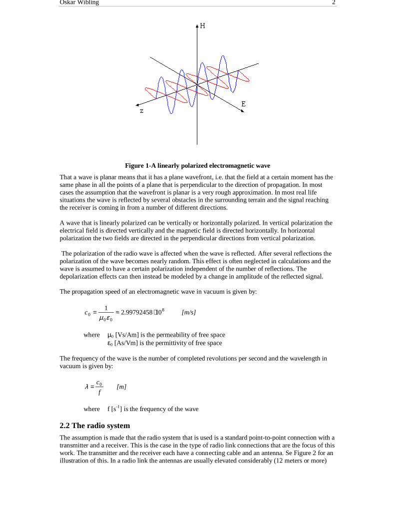
2.8.4 Modeling with cylindrical shapesA cylindrical obstacle is one that is curved in the direction of propagation and infinitely long in thehorizontal direction perpendicular to the direction of propagation. See Figure 8 for an illustration of thegeometry of a cylindrical obstacle.

Oskar Wibling 9

Figure 8 – Geometry of cylindrical obstacle model

Cylindrical shapes can be used to model obstacles that have a certain extent along the radio path. Theycan sometimes be of interest because extended obstacles cause a darker shadow of diffraction than dothin ones. This difference increases with the radius of the obstacle. A more common solution, however,is to use several thin obstacles to model extended geographical shapes.

2.8.5 Using an empirical clutter factorCalculating using clutter factors bears some resemblance to performing simple layer calculations.Clutter factors are used when the cause of a propagation effect cannot be described in the model, eitherbecause of lacking knowledge of the terrain or because an absurd amount of calculation time would beneeded to describe its influence correctly. This is for example the case when the terrain is not knownwith a high enough resolution.

In the present models and terrain databases, forests and buildings in many cases have to be viewed asclutter if they are in the near vicinity of a station, while they can be included in the model further outalong the radio path. The reason for this is that the propagation along the path can be described withoutdetailed knowledge of the terrain while the propagation near the stations demand knowledge aboutindividual houses and/or trees to be described correctly. The idea behind clutter factors is to describethe mean attenuation caused by obstacles. However, this does not describe the effect on the propagationin room and frequency correctly. There are many ways of calculating clutter factors. Some arecompletely empirical while others have a partially physical foundation.

3 Attenuation calculation methods

3.1 Free space attenuation model

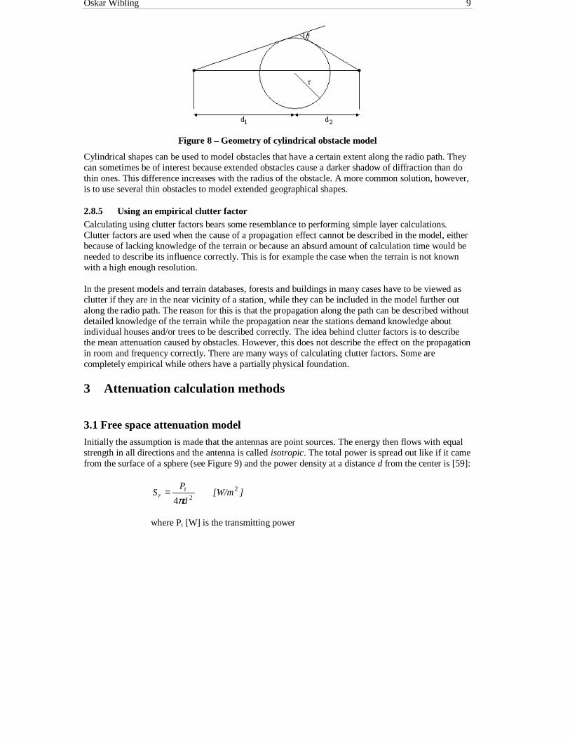
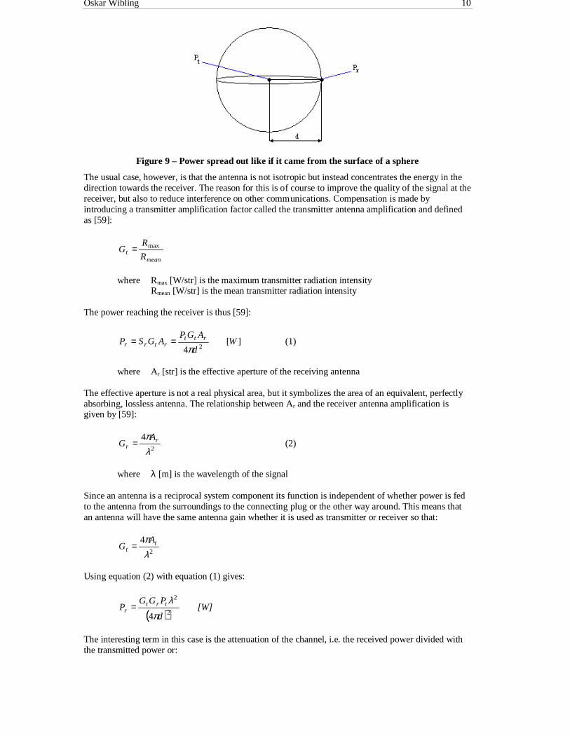
Initially the assumption is made that the antennas are point sources. The energy then flows with equalstrength in all directions and the antenna is called isotropic. The total power is spread out like if it camefrom the surface of a sphere (see Figure 9) and the power density at a distance d from the center is [59]:

][W/md

PS t

r2

2

4π=

where Pt [W] is the transmitting power

Oskar Wibling 10

Figure 9 – Power spread out like if it came from the surface of a sphere

The usual case, however, is that the antenna is not isotropic but instead concentrates the energy in thedirection towards the receiver. The reason for this is of course to improve the quality of the signal at thereceiver, but also to reduce interference on other communications. Compensation is made byintroducing a transmitter amplification factor called the transmitter antenna amplification and definedas [59]:

meant

R

RG max=

where Rmax [W/str] is the maximum transmitter radiation intensityRmean [W/str] is the mean transmitter radiation intensity

The power reaching the receiver is thus [59]:

][ 4 2

Wd

AGPAGSP rtt

rtrr π== (1)

where Ar [str] is the effective aperture of the receiving antenna

The effective aperture is not a real physical area, but it symbolizes the area of an equivalent, perfectlyabsorbing, lossless antenna. The relationship between Ar and the receiver antenna amplification isgiven by [59]:

2

4

λπ r

rA

G = (2)

where λ [m] is the wavelength of the signal

Since an antenna is a reciprocal system component its function is independent of whether power is fedto the antenna from the surroundings to the connecting plug or the other way around. This means thatan antenna will have the same antenna gain whether it is used as transmitter or receiver so that:

2

4

λπ t

tA

G =

Using equation (2) with equation (1) gives:

( )[W]

d

PGGP trt

r 4 2

2

πλ

=

The interesting term in this case is the attenuation of the channel, i.e. the received power divided withthe transmitted power or:

Oskar Wibling 11

( )2

2

4 d

GG

P

PA rt

t

r

πλ

==

Usually this is expressed in decibels (dB) as:

( ) ( ) [dB]d

GGAA rt 4

log10log10log102

101010

+==

πλ

Normally the propagation speed of electromagnetic waves in vacuum (see section 2.1) is used and thefollowing approximation is received:

( ) ( ) ( ) [dB]fdGGA rt log20log2055.147log10 101010 −−+≈

Here SI units (i.e. meters for distance and Hertz for frequency) have been used. Common practice,however, in radio science applications is to use kilometers (km) for distance and megahertz (MHz) forfrequency. If those units are used instead the following expression results:

( ) ( ) ( ) [dB]fdGGA rt log20log2045.32log10 101010 −−−≈

This amplification factor can be divided in two parts, one which is called the antenna gain and the otherwhich is called the free space attenuation, according to:

( ) ( ) ( )( ) [dB]fdGGA rt A-Alog20log2045.32log10 freegain101010 =++−≈

The free space attenuation is therefore given as:

( ) ( ) [dB]fdAfree log20log2045.32 1010 ++=

where d [km] is the distance between the stationsf [MHz] is the frequency

Note that this is an attenuation as opposed to an amplification. An alternative way to express it is as anegative amplification of the signal. In the following chapters the propagation factors will sometimesbe given as negative amplifications. It is important to always keep in mind if it is a negativeamplification (that is to be added to the signal power) or an attenuation (that is to be subtracted fromthe signal power) that is given.

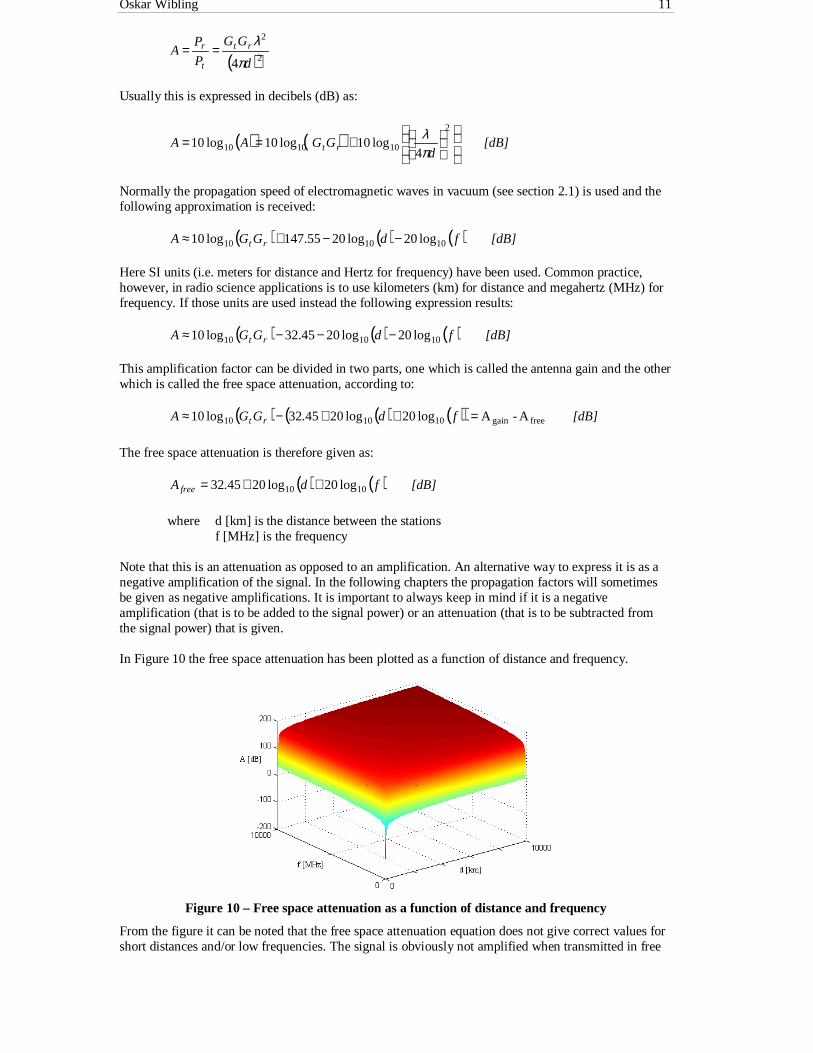
In Figure 10 the free space attenuation has been plotted as a function of distance and frequency.

Figure 10 – Free space attenuation as a function of distance and frequency

From the figure it can be noted that the free space attenuation equation does not give correct values forshort distances and/or low frequencies. The signal is obviously not amplified when transmitted in free

Oskar Wibling 12

space from one antenna to another independently of how closely they are positioned and/or how low afrequency is used.

3.2 Smooth spherical earth attenuation models

In these models the assumption is that the antennas are in fact mounted on a surface (the earth) but thatthis surface is completely smooth. Since the surface of the earth is a partially conducting surface it willinfluence the field and energy transport in several ways. Somewhat simplified it may be suggested thatthe field at the receiver is divided into three components [1](see Figure 11): Direct wave components,ground reflected wave components and surface wave components. These three components are oftenreferred to collectively as the ground wave.

Figure 11 – The three components of a radio wave propagating close to the surface of the earth

The direct wave and the ground reflected wave components together constitute the atmospheric wave.The surface wave, as the name implies, can only exist close to the surface of the earth and is ofimportance only if the height of the transmitting antenna is small compared to the wavelength.

Initially a plane earth model is used instead of a curved (spherical) earth as can be seen in Figure 12.The reason for doing this simplification is that it is much easier to perform calculations on a flatpropagation path as opposed to a curved one. This is in effect the same as modeling the earth as havingan effective radius of infinity.

Figure 12 – Plane earth model

The models developed under the assumption that the earth is flat are valid up to distances [37]:

3

1

12000λ<d

The first model that will be discussed is called the two-wave model, in which the surface wave isneglected. Since the electromagnetic field at the receiver is dominated by the direct and groundreflected waves at reasonably high frequencies this is an often used approximation.

The second model also takes the surface wave component into consideration which gives a more exactresult, particularly at lower frequencies.

Oskar Wibling 13

3.2.1 The two-wave modelThe two waves in this model are the atmospheric wave components, i.e. the direct wave and the groundreflected wave that affect each other (as discussed in section 2.7). This leads to a fluctuating behaviorin the signal strength at different distances from the transmitter.

When the wave is reflected by the surface it interacts electrically with the ground. The result is that thereflected wave is both phase shifted and attenuated. Since it is assumed that the transmitted signal hasa narrow bandwidth (see section 2.3) the fields will be roughly sinusoidal. The magnitude of theelectrical field component at the receiver then varies according to [1]:

( ) ( ) ( )( )φωρω +∆−+= ttEtEtE coscos 00

where ρ is the attenuation factor (including depolarization effects)φ is the phase shift caused by the ground reflectionE0 is the amplitude (field strength) of the direct wave according to the free spacemodel

Usually the difference in path length between the two wave components is considered so much smallerthan the total distance between the antennas that the additional free space attenuation caused by thisdifference is ignored.

If the ground is considered to be perfectly conducting (i.e. giving a lossless mirror reflection) theattenuation factor can be set to one and the phase shift set to π. This gives the magnitude of theelectrical field component at the receiver as:

( ) ( ) ( )ψωωψω +

∆=+= t

tEtEtE cos

2sin2cos 0 (3)

Using the notation in Figure 12 the difference in path length between the direct and reflectedcomponents is given as:

d

hhddd rt

dr2

≈−=∆

This results in a time difference of:

dc

hh

c

dt rt2

=∆=∆

Which used in (3) yields:

=

=

∆=

d

hhE

dc

hhE

tEE rtrt

λπωω 2

sin2sin22

sin2 000

The propagation factor (see section 2.3) is then given by:

[dB]d

h

d

h

d

hh

E

EF

rt

rtflat

44

5.0sin220log

2sin4log10log10

22

10

2102

0

2

10

⋅⋅=

=

=

=

λπ

λπ

λπ

(The last step was only performed to clarify the similarity between this equation and the onesin section 3.2.2.)

Oskar Wibling 14

In Figure 13 the propagation factor when using the two-wave model has been plotted as a function ofdistance and frequency for both transmitter and receiver antenna heights of 12 meters.

Figure 13 - Propagation factor as a function of frequency and distance when using the two-wavemodel

3.2.2 A model that also accounts for the surface waveTo model the complete ground wave (direct wave, ground reflected wave and surface wave) a moreadvanced analysis, that includes knowledge of the properties of the ground and reflecting surfaces, isneeded.

One such model initially assumes both the antennas to be at zero height, i.e. on the surface and uses socalled height gain functions [42] to account for the situation where the antennas have been elevatedfrom the ground. The model can, according to Holm[28] and Blomquist [13], be written as:

( ) ( )( ) ( )

=

rt

rrtt

dwdw

hfhf

d

EE

ζζ

ζζ

,,2

,,sin

2 0

where E0 is the field strength at unit length in free spaced [m] is the distance between the antennasf(h, ζ) are height gain functions

The subscripts t and r indicate transmitter and receiver respectively.

The height gain functions are given by:

( )

+

+=

onpolarizati horizontalat 2

1

onpolarizati lat vertica 2

1

,

λζπλ

ζπ

ζhj

jh

hf

where ζ is the normalized surface impedance

|w(d, ζ)| are given by:

Oskar Wibling 15

( )

=onpolarizati horizontalat

1

onpolarizati lat vertica

, 2

2

ζλπ

ζλ

π

ζd

d

dw

where ζ is the normalized surface impedance

The normalized surface impedance is given by:

−

−

=onpolarizati horizontalat

1

1

onpolarizati lat vertica 1

c

c

c

ε

εε

ζ

where εc is the complex constant of dielectricity given by:

jrc λσεε 60−=

where εr is the relative permittivity of the surfaceσ [S/m] is the relative conductivity of the surface

An approximation that can now be made is to neglect the conductivity of the surface. It is accurate inmost practical cases except over sea water for the lowest frequencies. The complex constant ofdielectricity is then set equal to the relative permittivity of the surface. The approximation yields thesame expression that Ladell [37] writes about:

( )( )( )( ) [dB]BABAF rrttflat 5.0sin2log20 10 ++=

The functions At, Ar, Bt and Br are given as:

( ) ( )1 and

1 ,

4 ,

4

,,

22

−⋅⋅

=−⋅

⋅=

⋅=

⋅=

rr

rr

tr

tt

rr

tt d

CB

d

CB

d

hA

d

hA

επλ

επλ

λπ

λπ

With the functions Ct and Cr given by:

Vertical polarization: 2rC ε=

Horizontal polarization: 1=C

(Note that C at the transmitter is calculated using the relative permittivity of the surface at thetransmitter and correspondingly for the receiver.)

Ladell [37] reports an error of less than 1.5 dB for distances 3131012 λ⋅⋅≤d .

If the conductivity is not disregarded the propagation factor can still be expressed as:

( )( )( )( ) [dB]BABAF rrttflat 5.0sin2log20 10 ++=

With the same functions At and Ar as before but with other functions Bt and Br according to:

Vertical polarization:( )

( )22

232 42403600

bad

hbahB rr

++±+

=π

πεσπλσλλε

Oskar Wibling 16

Horizontal polarization: ( )22

4

bad

hbB

+±=

ππλ

(Note that B at the transmitter is calculated using the relative permittivity and conductivity ofthe surface at the transmitter and correspondingly for the receiver.)

In these equations a and b represent the real and imaginary parts of z in the expression:

( ) jz r λσε 601 −−=

That is:

( ) ( )

( ) ( )

+−+−=

+−+−=

2

360011

2

360011

222

222

σλεε

σλεε

rr

rr

b

a

(Note that a and b at the transmitter are calculated using the relative permittivity andconductivity of the surface at the transmitter and correspondingly for the receiver.)

In Figure 14 propagation factor curves for the frequency 1.2 GHz with (dashed line) and without (solidline) neglecting the conductivity of the surface have been drawn for an earth-sea boundary as a functionof distance. The relative permittivities and conductivities used are εr,t = 15, σt = 0.005, εr,r = 80, σr = 4(where the extra subscripts t and r stand for transmitter and receiver respectively). The antennaelevations have been set to 12 meters for both the transmitter and the receiver.

Figure 14 - Propagation factor as a function of distance when using a smooth, flat earth modelthat accounts for the complete ground wave with (dashed line) and without (solid line) neglecting

the conductivity of the surface

The relative permittivities and conductivities of the surface can be selected by consulting the table inAppendix A.

3.2.3 Accounting for the curvature of the earthBy applying a curvature correction the flat-earth models can be extended to cover longer distances.Blomquist [11] has constructed a model in which the curvature correction is given by:

Oskar Wibling 17

( )

−+=⇒<≤−=⇒<

[dB] 2.10log107.62532.0

[dB] 758.2532.0

10 xxYx

xYx

where the normalized distance, x, is given by:

( ) 320

312 −⋅

⋅= Rkdx

λπ

where R0 [m] is the radius of the earth (approximately 6370 km)k is the earth radius factor (4/3 for standard radio atmosphere)

Figure 15 shows the curvature correction as a function of the parameter x.

Figure 15 – The curvature correction as a function of the parameter x

The total propagation factor for a smooth, spherical earth model is then written as:

[dB]YFF flatsmooth +=

Ladell [37] claims that the correction factor can be used for distances up to x = 4.5 with an error of lessthan 1.5 dB. For a frequency of 1.2 GHz that corresponds to a distance of approximately 6.4 km.

3.3 Single knife-edge diffraction attenuation model

If the terrain between transmitter and receiver is modeled with a single knife-edge a closed expressionfor the propagation factor can be given. See Figure 16 for an illustration of the situation. The angle α iscalled the angle of diffraction.

Oskar Wibling 18

Figure 16 - Single knife-edge model

Further the assumption is made that the transmitter and receiver are both far away from the obstaclethereby considering the wave to be approximately planar at the obstacle. More precisely theassumptions are that h<<d1, h<<d2 and that h>>λ.

Huygens’ principle states that wavelets originating from all points on a plane through the base and topof the obstacle and normal to the direction of propagation propagate into the shadow region (i.e. theregion behind the obstacle that is not reached by a straight line from the transmitter) and that the fieldat any point in this region will be the resultant of the interference of all these wavelets. Hence, therewill not only be a direct wave (along the solid line in Figure 16), but also some weaker fieldcomponents illuminating the shadow region.

Now return to Figure 16. The excess path length that the diffracted beam (solid and then dashed line)travels in comparison to an imaginary beam going through the obstacle (dashed line) can then becomputed as [1]:

( )[m]

dd

ddhd

2 21

212 +

≈∆

Between the two waves there is therefore a phase difference [1]:

2

2

2v

d πλ

πφ =∆=

were λ is the wavelength of the diffracted wavev is the Fresnel-Kirchhoff diffraction parameter

The Fresnel-Kirchhoff diffraction parameter is given by [48]:

+⋅=

21

112

ddhv

λ

The field strength at the receiver is given as the sum of all the secondary Huygens sources in the planeabove the obstruction and can be expressed as (see [39] and [48] for more details):

∫∞

∆−⋅=+=

v

jtj

eFdtej

E

E φπ 2

2

0 2

)1((4)

F and ∆φ are given by [39]:

Oskar Wibling 19

45.0

5.0tan

4sin2

5.0

1 πφ

πφ

−

++=∆

+∆

+=

−

C

S

SF

C and S in the last two equations are known as the Fresnel integrals and given by [39]:

∫

∫

=

=

v

v

dxxS

dxxC

0

2

0

2

2sin

2cos

π

π

The complex Fresnel integral (4) can alternatively be written on the form [48]:

( ) ( ) ( )

−−

−+= vSjvC

j

E

E

2

1

2

1

2

1

0

Parsons [48] suggests that part of this expression is studied, more specifically the following integral:

( ) ( ) ∫−

=−v tj

dtevjSvC0

22π

Plotting it in the complex plane with C as the abscissa and S as the ordinate results in a curve known asCornu’s spiral of which part is shown in Figure 17. Parsons writes that Cornu’s spiral gives a visualindication of how the magnitude and phase of E varies as a function of the Fresnel parameter v.

Figure 17 – Part of Cornu’s spiral

The propagation factor when using a diffraction model is, as explained in [5] and [32], then given by:

( ) [dB]FF ndiffractio log20=

Since the solution for F involves solving Fresnel integrals it makes the computation process quitedifficult. Various approximations of Fdiffraction are available that enable the diffraction loss to becalculated much more easily. Lee [39] suggests the following five expressions for different values ofthe parameter v:

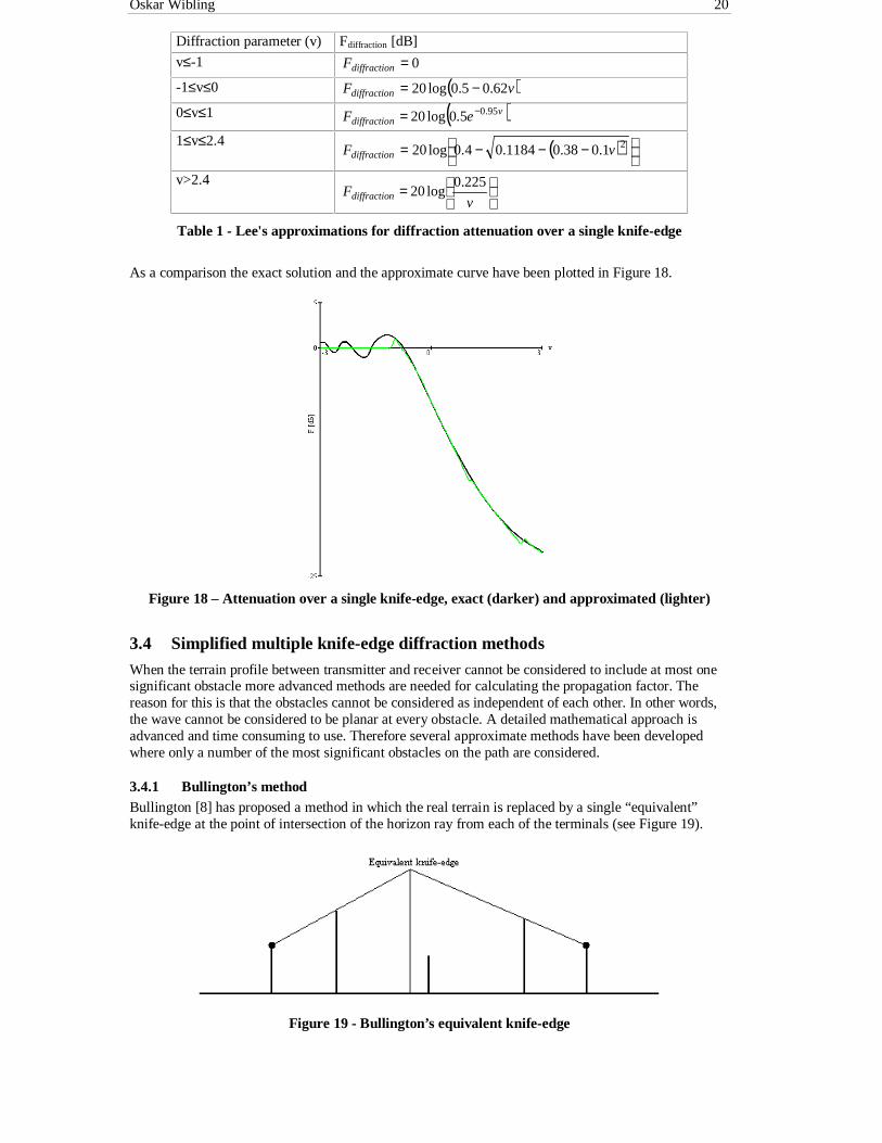
Oskar Wibling 20

Diffraction parameter (v) Fdiffraction [dB]

v≤-1 0=ndiffractioF

-1≤v≤0 ( )vF ndiffractio 62.05.0log20 −=

0≤v≤1 ( )vndiffractio eF 95.05.0log20 −=

1≤v≤2.4 ( )

−−−= 21.038.01184.04.0log20 vF ndiffractio

v>2.4

=

vF ndiffractio

225.0log20

Table 1 - Lee's approximations for diffraction attenuation over a single knife-edge

As a comparison the exact solution and the approximate curve have been plotted in Figure 18.

Figure 18 – Attenuation over a single knife-edge, exact (darker) and approximated (lighter)

3.4 Simplified multiple knife-edge diffraction methods

When the terrain profile between transmitter and receiver cannot be considered to include at most onesignificant obstacle more advanced methods are needed for calculating the propagation factor. Thereason for this is that the obstacles cannot be considered as independent of each other. In other words,the wave cannot be considered to be planar at every obstacle. A detailed mathematical approach isadvanced and time consuming to use. Therefore several approximate methods have been developedwhere only a number of the most significant obstacles on the path are considered.

3.4.1 Bullington’s methodBullington [8] has proposed a method in which the real terrain is replaced by a single “equivalent”knife-edge at the point of intersection of the horizon ray from each of the terminals (see Figure 19).

Figure 19 - Bullington’s equivalent knife-edge

Oskar Wibling 21

As seen in the figure the method of an equivalent knife-edge only uses a maximum of two obstacles inthe terrain profile to calculate the new single knife-edge. The method is sometimes used in connectionwith the elevation method for selecting significant heights (see section 3.6.2).

After the equivalent height has been calculated the diffraction loss is computed by using the method fora single knife-edge. This method has the advantage of simplicity, but since important obstacles aresometimes ignored it can yield large prediction errors. It works best for a path with only two significantobstructions and is known to generally underestimate the path loss.

3.4.2 The Epstein-Peterson methodThe Epstein-Peterson model [22] considers each knife-edge individually and sums the contributions.The first loss is calculated between the transmitter and the second obstruction on the path. The secondloss is calculated between the first and third obstructions on the path, and so on (see Figure 20).

Figure 20 - The Epstein-Peterson model

Given the situation in the figure (with three heights) the following parameters are received:

First knife-edge:

==

+−=

22

11

21

121

dD

dD

dd

dhhH

Second edge:

( )

==

+−−−=

32

21

32

21312

dD

dD

dd

dhhhhH

Third edge:

==

+−=

42

31

43

423

dD

dD

dd

dhhH

The parameters H, D1 and D2 are then used in the method for a single knife-edge to calculate the threeattenuations. The attenuations are added to receive the total propagation factor.

For two obstacles that are closely spaced, the Epstein-Peterson method has been shown to give largeprediction errors. However, by using a correction [48] that is added to the loss originally calculated theperformance can be improved.

3.4.3 The Deygout methodThe Deygout model [18] works by initially estimating the loss when considering only the dominantknife-edge. The other losses, due to the other edges, are calculated with respect to the dominant edge(see Figure 21).

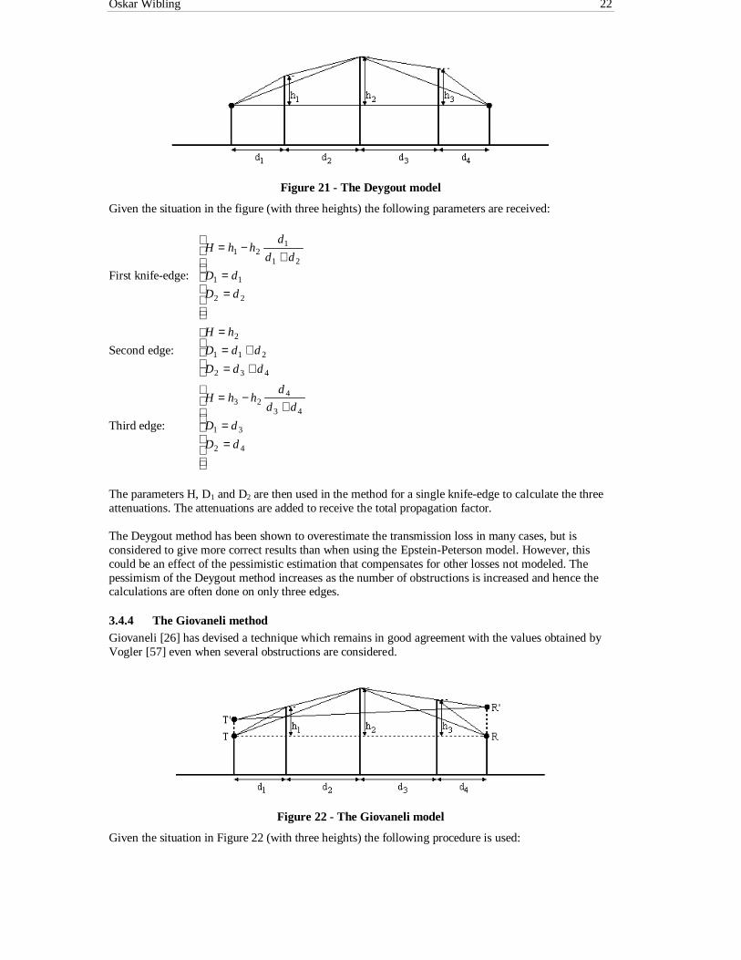
Oskar Wibling 22

Figure 21 - The Deygout model

Given the situation in the figure (with three heights) the following parameters are received:

First knife-edge:

==

+−=

22

11

21

121

dD

dD

dd

dhhH

Second edge:

+=+=

=

432

211

2

ddD

ddD

hH

Third edge:

==

+−=

42

31

43

423

dD

dD

dd

dhhH

The parameters H, D1 and D2 are then used in the method for a single knife-edge to calculate the threeattenuations. The attenuations are added to receive the total propagation factor.

The Deygout method has been shown to overestimate the transmission loss in many cases, but isconsidered to give more correct results than when using the Epstein-Peterson model. However, thiscould be an effect of the pessimistic estimation that compensates for other losses not modeled. Thepessimism of the Deygout method increases as the number of obstructions is increased and hence thecalculations are often done on only three edges.

3.4.4 The Giovaneli methodGiovaneli [26] has devised a technique which remains in good agreement with the values obtained byVogler [57] even when several obstructions are considered.

Figure 22 - The Giovaneli model

Given the situation in Figure 22 (with three heights) the following procedure is used:

Oskar Wibling 23

First the main obstacle is identified and then two observation planes T’T and R’R are constructed as canbe seen in the figure. The attenuation is calculated for the main obstacle considering the height abovethe line between the "new" stations T’ and R’. After that the attenuation is calculated for the pathbetween the original transmitter T and the main obstacle. Lastly, the attenuation is calculated for thepath between the main obstacle and the original receiver R. The following parameters are thusreceived:

First knife-edge:

==

+−=

22

11

21

121

dD

dD

dd

dhhH

Second edge:

( )

+=+=

++++′−′+′−=

432

211

4321

212

ddD

ddD

dddd

ddRTThH

where T’ and R’ are given by:

( )

( )

−−=′

−−=′

3

4323

2

1121

d

dhhhR

d

dhhhT

Third edge:

==

+−=

42

31

43

423

dD

dD

dd

dhhH

The parameters H, D1 and D2 are used in the method for a single knife-edge to calculate the threeattenuations. The attenuations are added to receive the total propagation factor.

If an obstacle is sub-path, i.e. below the level from which its effective height is calculated, then theeffective height will have a negative value.

Giovaneli writes that the procedure for three or more obstacles takes into account the deflection anglesat the edges, by extending the construction outlined for three edges. First, the main hill is selected andobservation planes through points T and R introduced. The effective height of the main obstacle is thenobtained by considering the intersection between the line T’R’ and the vertical line joining the top of thehill with line TR. The same construction can be extended to the propagation paths at both sides of theprincipal hill, by considering a new observation plane at the position of this hill. If there are, forexample, two hills between the transmitter and the main obstacle, it must be determined first which onehas the larger individual loss. Taking into account the correct deflection angle for this hill, thecorresponding effective height with respect to the new observation plane is obtained. The procedurecould be repeated systematically.

3.4.5 Other simplified modelsSome other models that will not be described thoroughly, but are worth mentioning here are:

• Picquenard’s model - Lee [39] writes that in Picquenards model, the limitations that were apparentin Bullington’s and Epstein-Peterson’s models are not present. The height of one obstruction is

Oskar Wibling 24

obtained first, without regard to the second obstruction, as though it did not exist. The height of thesecond obstruction is then measured by drawing a line from the top of the first obstruction to thereceiver. Lee recommends this method for general use.

• The Japanese model - This technique, proposed by the Japanese postal service, is similar inconcept to the Epstein-Peterson method. The difference is that in computing the loss due to eachobstruction the effective source is not the top of the preceding obstruction, but the projection of thehorizon ray through that point onto the plane of one of the terminals.

• The Eklund-Nilsson model -Eriksson [23] writes that a method with a solid physical foundation,without being too calculation intensive, is the method by Eklund and Nilsson [20]. In that method,the illumination is first calculated in a vertical section between two primary knife-edges, and thenHuygen’s principle is used to calculate the field strength at the receiver. One secondary obstacle onboth sides of the primary obstacles can be accounted for, which means that a maximum of sixobstacles can be used in the calculation. To get integrals that are simple to solve the illumination inthe vertical sections are approximated with simple functions. Eriksson writes that the method hasbeen compared with measurements on a few paths and shows relatively good results forfrequencies over 100 MHz. For lower frequencies, the method gives an attenuation which is toolow, but this is a common error in all knife-edge diffraction methods, since the attenuation due todiffraction over spherical earth is starting to dominate over the knife-edge diffraction.

3.5 The Vogler knife-edge diffraction method

The Vogler method [54][57] can correctly predict diffraction for a series of up to ten knife-edges. Ituses numerical methods to solve the integral functions that appear in the expressions for theattenuation. The method is much more calculation intensive than the simpler methods discussed earlier.It is therefore more interesting to use in cases when fast calculations are not a necessity and moreaccurate results are needed.

3.5.1 The calculation method

As before the propagation factor is defined as:

( ) [dB]FF ndiffractio log20=

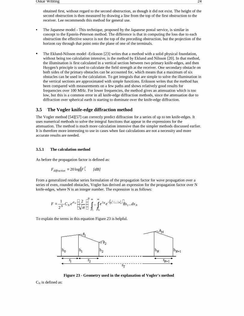
From a generalized residue series formulation of the propagation factor for wave propagation over aseries of even, rounded obstacles, Vogler has derived an expression for the propagation factor over Nknife-edges, where N is an integer number. The expression is as follows:

( )∫ ∫∞ ∞

++−

=

1

221 ......

2

2

11

...2

β β

σ

πN

NNN

xxgN

NNdxdxeeeCF

To explain the terms in this equation Figure 23 is helpful.

Figure 23 - Geometry used in the explanation of Vogler's method

CN is defined as:

Oskar Wibling 25

( )( ) ( )

≥+++

=

=

+2Nhen w

...

...

1Nn whe 1

13221

32

NN

TNN

rrrrrr

rrrrC

g is defined as:

( )( )

≥−−

== ∑

−

=++

1

111 2Nhen w

1N when 0N

nnnnnn xx

gββα

σn is a pure imaginary number defined as:

222

21 ... NN βββσ +++=

αn is a measurement of how asymmetrically the obstacles are placed and is defined as:

( )( )211

2

+++

+

++=

nnnn

nnn rrrr

rrα for n = 1, …, N-1

βn is defined as:

( )1

1

2 +

+

+=

nn

nnnn rr

rikrθβ for n = 1, …, N

where k is the wave number (k = 2π/λ)

θn is the diffraction angle and is defined as:

−+

−=

+

+−

1

11 arctanarctann

nn

n

nnn r

hh

r

hhθ for n = 1, …, N

Since the integral in the equation for F above is impossible to solve analytically except in some specialcases, Vogler has proposed a numerical method to use. The equation is then written on the form:

∑∞

==

02

1

mmNN

IeCF Nσ

This sum has to be limited to prevent some of the numbers in the calculation of Im from becoming toolarge. Svensson [54] proposes a maximum value of m = 170. That many terms may, however, not needto be calculated. By using a stopping criteria like for example the ratio test [52] the calculations arespeeded up and the risk of overflow is reduced. (The ratio test works by dividing the absolute value ofthe most recentely added term with the absolute value of the total sum thus far and comparing this ratiowith a chosen stopping number.) Svensson [54] also uses an extrapolation of the sum using Aitkens δ2-process [50] in two steps to limit the number of terms needed to be calculated even more.

Im is defined as:

When N = 2: ( ) ( )211 ,,!2 ββα mImImI mmm =

When N ≥ 2: ( ) ( )∑=

− −=m

p

pmmm mpCpmII

011 ,,2,2 βα

Oskar Wibling 26

The function C(…) is defined recursively as:

( ) ( )( ) ( ) ( )piLNCimI

ip

immpLNC LN

ipLN

p

i

,,1,!

!,,

0

+−−

−−=− −

−−

=∑ βα

for 2 ≤ L ≤ N-2 when N ≥ 4

The starting value for the recursion is:

( ) ( ) ( )NNiN iIpIppiNC ββα ,,!,,1 11 −−=−

which is also used to calculate C(2, p, m) when N = 3.

I(p, β) is the recurring integral of the error function and can be defined as:

( ) ( )∫∞

−=p

dttpIpI ,1, β

I(0, β) is the complementary error function:

( ) ∫∞

−=βπ

β dteerfc t22

Vogler has devised four different methods for calculating I(p, β) depending on the values of p and β.The reason for using four different methods is their different regions of convergence.

• Method A

When |β| < 0.8 and p < 10:

( ) ( ) ( ) ( )∑∑∑∞

=

∞

=

∞

= −−=

−+Γ

−=000

,,

21!2

1,

r

or

r

er

r rp

rr

pTpTrp

r

pI ββββ

where Γ is the gamma function

Γ is defined as:

( ) ∫∞

−−=Γ0

1 dtetx tx when Re(x) > 0

The two functions T are defined recursively as:

( ) ( )( ) ( )

( ) ( )( ) ( )βββ

βββ

,12

21,

,12

22,

1

2

1

2

pTrr

rppT

pTrr

rppT

or

or

er

er

−

−

−

−+=

−

−+=

Using the starting values:

Oskar Wibling 27

( )

( )

+

Γ=

+Γ

=

2

12

2,

2

22

1,

0

0

ppT

ppT

p

o

p

e

ββ

β

• Method B

When |β| < 0.8 and p ≥ 10:

( )

−

+Γ

= 22

2

22

,

2

ββ

βV

p

ep

epI

The function V(Z) is defined as:

( ) ( )∑

=

+

++−=9

1

2

12

2

12

qq

q

p

ZgpZZV

The functions g are defined as:

( )

( )( )

( )( )

( )

( )

( )( )

−+−=

+−=

+−=

−=

−=

=

+−=

−=

−=

11739

848

957

626

735

44

53

22

31

11

28120

3

575

1684

9

1026

2

193

169

7

4

3

16

2

5

2

3

2

ZZZZg

ZZZg

ZZZZg

ZZZg

ZZZg

ZZg

ZZZg

ZZg

ZZg

• Method C

When |β| ≥ 0.8 and Re(β) ≥ 0:

( ) ( )( )ββ

πβ

β

1

2

2,

−

−=

w

wepI

pfor p = 0, 1, …

The helper functions w are defined recursively as:

Oskar Wibling 28

( ) ( ) ( ) ( )( )βββµβ µµµ 1222 ++ ++= www for µ = ν, ν − 1, ..., −1

( )( ) αββ

ν

ν

≡≡

+

+

1

2 0

w

w

where α is an arbitrary, small, positive constant

The method was developed by Gautschi and is based on a technique by J.C.P. Miller. Gautschi hasexamined how large ν needs to be to get a relative error in I(p, β) that has an absolute value lessthan 0.00000001. He has found that:

2758.6

+≥

βν p

However, ν might still need to be limited upwards so that w-1 does not become a too large numberfor the computer to handle. Svensson [54] has proposed a maximum value of 240 for ν and writesthat the limit has an insignificant effect on the result.

• Method D

When |β| ≥ 0.8 and Re(β) < 0:

( ) ( ) ( ) ( )( )βββ −−−= ,21, pIApI pp

The function Ap(β) is defined as:

( )( )∑

=

−

−=

2

0

2

!2!4

p

tt

tp

ptpt

Aββ

(This formulation of the method is the one used by Svensson [54].)

3.5.2 Example calculationsThe following two examples are used by Vogler [57]:

(1) A 30 km propagation path is assumed to have two fixed knife-edges at distances of 10 km and 20km from the transmitter with heights h1 = h3 = 100 m. Both the transmitter and the receiver lie onthe reference plane from which heights are measured, i.e. h0 = h4 = 0. A third knife-edge withvariable height, h2, is placed in the middle of the path at 15 km. The frequency used is 100 MHzand a plot of the attenuation factor is given in Figure 24.

Oskar Wibling 29

Figure 24- Vogler example calculation 1

In the figure the curve for a path with only a single knife-edge at the same position as the variableknife-edge has been plotted as a reference. It can be observed that as the height of the middleknife-edge increases the attenuation factor goes towards the value for a single knife-edge asexpected.

(2) A 50 km propagation path with the transmitter at height ht = 0 and the receiver with variable heighthr. A number of knife-edges are evenly spaced in the region 0 - 42 km from the transmitter. Theknife-edges have heights hi = 420(i/N) where N is the total number of knife-edges. The heights ofthe additional knife-edges are such that the tops just graze the direct ray between the transmitterand the knife-edge at 42 km. The frequency used is 500 MHz and a plot of the attenuation factor isgiven in Figure 25.

Figure 25 - Vogler example calculation 2

3.6 Selecting the heights for diffraction attenuation calculations

Two methods for selecting the heights when performing diffraction attenuation calculations will bediscussed. They are the Fresnel zone approach and the Elevation method. An important point beforeexplaining the two methods further is that the heights to use in a diffraction attenuation calculationshould not be allowed to be positioned too closely together. The reason for this is that if, for example,three heights is set to the maximum number to use in the calculations these three heights may all beselected very close to each other to model a certain obstacle. Other obstacles on the path are thenneglected and the simplified model does not do a good job in modeling the real situation. A minimaldistance between obstacles is given by Svensson [54] as:

λ⋅−= Cdmin

where C is a negative constant

Oskar Wibling 30

Svensson writes that C = -500 has proven to be a good compromise for most paths. A check for thiscondition can be included in the algorithms to prevent them from selecting the heights too closely. Aproblem that might follow when performing this check is that the algorithms may not be able to findthe requested amount of heights.

3.6.1 The Fresnel zone approachA recursive method can be used to find the heights before starting the calculations or the heights can beselected and the attenuation calculated continuously. The approach is basically the same and theprocedure is as follows:

(1) The path between transmitter and receiver is examined. The radius of the first Fresnel zone iscalculated on this path and the ratio between the height that is inside the first Fresnel zone at aspecific point and the radius of the first Fresnel zone at that point is calculated. If the height in apoint is below the first Fresnel zone that point is disregarded. See Figure 26 for an illustration ofthis. The selected height is indicated with a vertical line in the figure.

Figure 26 – A radio path with height profile and first Fresnel zone

The point that gave the largest ratio is selected and reported as the most significant height in thisstep. If no heights were found or if enough heights have been found the algorithm ends.

(2) The most significant height that was found is used as receiving antenna for the left path and astransmitting antenna for the right path as shown in Figure 27. The selected heights in the next stepare indicated with vertical lines in the figure. Note that a different scaling has been used in the leftand right path and also in the figure above. This has been done to fit as much as possible into thegraphics window and will hopefully not confuse the reader.

Figure 27 – The division of the path into two new paths

The two new paths are used as input and the algorithm continues from step (1).

Using this recursive method a maximum number of 1, 3, 7, 15 etc. heights can be found depending onif the algorithm is allowed to go to depths 1, 2, 3, 4 etc.

3.6.2 The elevation methodA version of the elevation method that returns at most three significant heights will be described here.The method is often used to select heights for use by some of the simplified knife-edge diffractionattenuation calculation methods in which at most three heights are considered. The method works asfollows:

(1) The elevation from the transmitter to the heights of all the points on the path between transmitterand receiver are examined as shown in Figure 28. The point that gave the highest elevation angle isstored as the first most significant height. The elevation of the first most significant height isillustrated in Figure 28 by a solid line. If no first most significant height is found the algorithmends and reports no found significant heights.

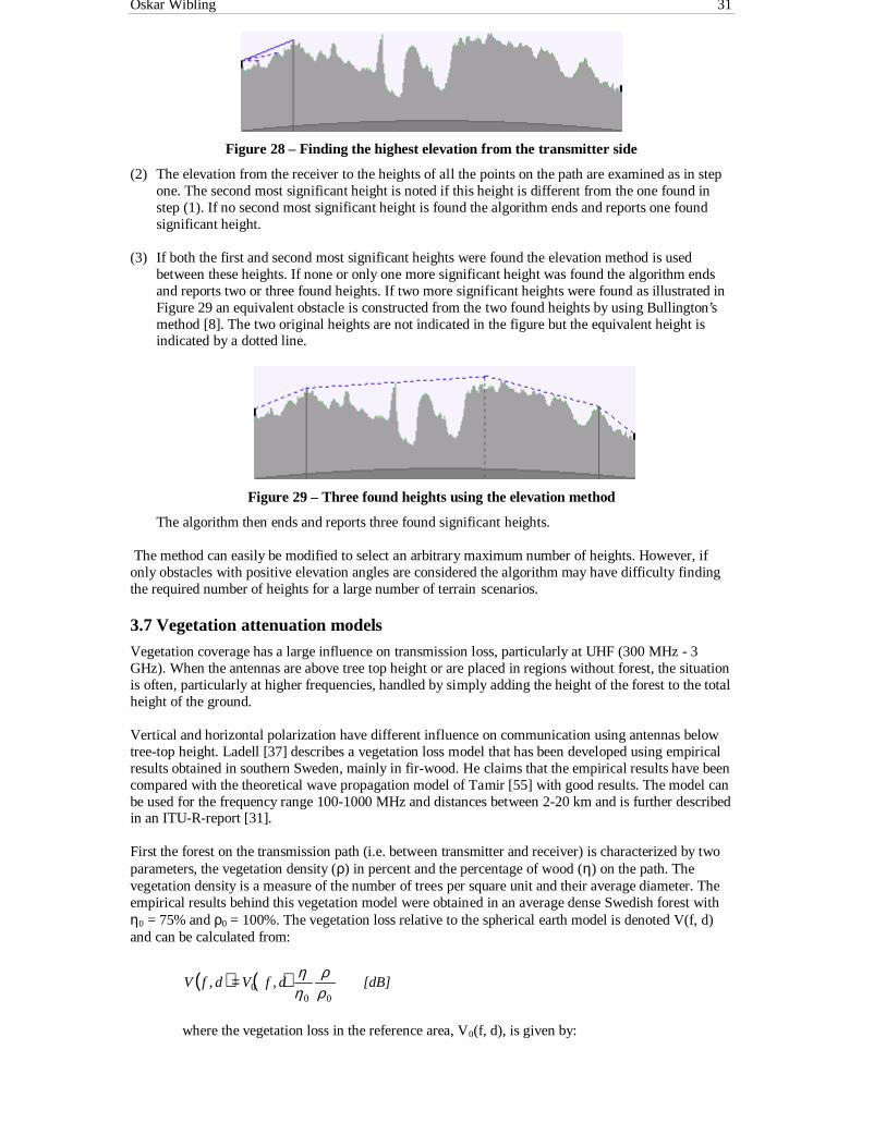
Oskar Wibling 31

Figure 28 – Finding the highest elevation from the transmitter side

(2) The elevation from the receiver to the heights of all the points on the path are examined as in stepone. The second most significant height is noted if this height is different from the one found instep (1). If no second most significant height is found the algorithm ends and reports one foundsignificant height.

(3) If both the first and second most significant heights were found the elevation method is usedbetween these heights. If none or only one more significant height was found the algorithm endsand reports two or three found heights. If two more significant heights were found as illustrated inFigure 29 an equivalent obstacle is constructed from the two found heights by using Bullington’smethod [8]. The two original heights are not indicated in the figure but the equivalent height isindicated by a dotted line.

Figure 29 – Three found heights using the elevation method

The algorithm then ends and reports three found significant heights.

The method can easily be modified to select an arbitrary maximum number of heights. However, ifonly obstacles with positive elevation angles are considered the algorithm may have difficulty findingthe required number of heights for a large number of terrain scenarios.

3.7 Vegetation attenuation models

Vegetation coverage has a large influence on transmission loss, particularly at UHF (300 MHz - 3GHz). When the antennas are above tree top height or are placed in regions without forest, the situationis often, particularly at higher frequencies, handled by simply adding the height of the forest to the totalheight of the ground.

Vertical and horizontal polarization have different influence on communication using antennas belowtree-top height. Ladell [37] describes a vegetation loss model that has been developed using empiricalresults obtained in southern Sweden, mainly in fir-wood. He claims that the empirical results have beencompared with the theoretical wave propagation model of Tamir [55] with good results. The model canbe used for the frequency range 100-1000 MHz and distances between 2-20 km and is further describedin an ITU-R-report [31].

First the forest on the transmission path (i.e. between transmitter and receiver) is characterized by twoparameters, the vegetation density (ρ) in percent and the percentage of wood (η) on the path. Thevegetation density is a measure of the number of trees per square unit and their average diameter. Theempirical results behind this vegetation model were obtained in an average dense Swedish forest withη0 = 75% and ρ0 = 100%. The vegetation loss relative to the spherical earth model is denoted V(f, d)and can be calculated from:

( ) ( ) [dB]dfVdfV ,,00

0 ρρ

ηη=

where the vegetation loss in the reference area, V0(f, d), is given by:

Oskar Wibling 32

( ) ( ) ( ) ( )( )( ) ( ) ( )( )

−++−−++−

=pol.) (Vert. [dB] 2loglog45log5.150.46

pol.) (Hor. [dB] 2loglog45log8.96.29,

101010

1010100 fdf

fdfdfV

where f [MHz] is the frequencyd [km] is the distance

For distances, d, below 2 km V0 should be calculated for a distance of 2 km and the result in dBmultiplied by 0.5d. For distances above 20 km the value calculated for 20 km should be used.

The model has been shown [43] to overestimate the attenuation for long paths with large amounts offorest and also to underestimate the attenuation for high frequencies.

Tamir [55][56] has developed a lateral wave model that has a limited frequency coverage (2 - 200MHz) but could be useful as a more exact method in the lower frequency range. Tamir has shown thatthe wave propagation in forests for longer distances, mainly is by a lateral wave propagating over thetreetops in the border region between forest and air. During the propagation energy continuously"leaks" down to the forest thereby contributing to the field there. The direct wave, that propagatesthrough the forest, is attenuated rather quickly. Models for the transmission loss when both stations arein the forest, i.e. below treetop height, have been presented by Dence and Tamir [17]. Eriksson [23]writes that a difficulty when using the model is the large effect the dielectric properties of the forest (εr

and σ) have on the attenuation. These parameters are very hard to predict in practice and depend on thethickness and composition of the forest and the polarization of the radio wave. Tamir has alsodeveloped the model to handle the case in which only one of the stations is in the forest and the otherstation is either above the forest or beyond the forest area. Mixed regions, i.e. paths where only parts ofthe propagation path is in forest, are also said to be able to be treated with the model.

3.8 Built up area attenuation models

Prediction models for urban areas have been a subject of extensive studies in recent years. The generalmethod seems to be to collect basic data and then try to adjust a model to fit these data as well aspossible. The problem is that a model that works well for a given set of data may not work at all whenapplied to new data. This could perhaps be a new area of application for neural networks. A neuralnetwork could be trained with urban data and the results might very well be satisfactory.

Returning to the current models, Ladell [37] claims that the semi-empirical model for urban loss byAllsebrook and Parsons [2] and Ibrahim and Parsons [29] is of particular interest.

Ibrahim and Parsons [29] write that an attempt has been made to develop an alternative predictionmethod which takes into account, in addition to other factors, land usage and degree of urbanization,since experiments have established their influence on the value of the path loss. Their models weredeveloped using experimental data from field trials in London. The base station with the transmittingantenna was located 46 m above local ground level and the receiving antenna was mounted on anautomobile driving through the streets at a height of 2.5 m above ground level. It can therefore besuspected that the model is best suited to use when either the transmitting or receiving antenna isplaced inside the urban area at a fairly low height and when most of the radio path is surrounded bybuildings. The frequencies used were 168, 455 and 900 MHz and hence the region of validity for themethods can be suspected to be approximately 100 - 1000 MHz.

Two possible approaches were tried by Ibrahim and Parsons. The first was to derive an empiricalexpression for the path loss based on multiple regression analysis and the second was to start from thetheoretical plane-earth equation and to correlate the excess path loss with the parameters likely toinfluence it. The main difference between the two methods is that in the second one a fourth-powerrange dependence law is assumed a priori.

In the semi-empirical model by Ibrahim and Parsons the best fit equation for the excess clutter loss is:

[dB]KHLf

Furban 34.018.040

20 +−++=

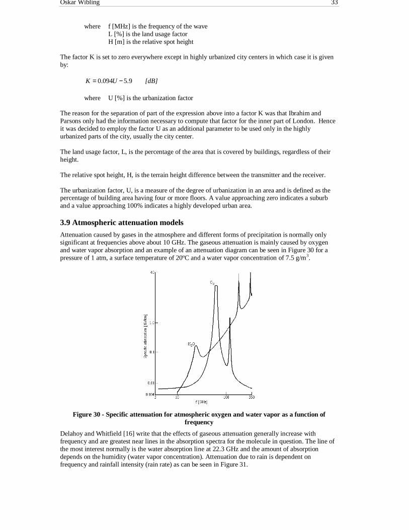
Oskar Wibling 33

where f [MHz] is the frequency of the waveL [%] is the land usage factorH [m] is the relative spot height

The factor K is set to zero everywhere except in highly urbanized city centers in which case it is givenby:

[dB]UK 9.5094.0 −=

where U [%] is the urbanization factor

The reason for the separation of part of the expression above into a factor K was that Ibrahim andParsons only had the information necessary to compute that factor for the inner part of London. Henceit was decided to employ the factor U as an additional parameter to be used only in the highlyurbanized parts of the city, usually the city center.

The land usage factor, L, is the percentage of the area that is covered by buildings, regardless of theirheight.

The relative spot height, H, is the terrain height difference between the transmitter and the receiver.

The urbanization factor, U, is a measure of the degree of urbanization in an area and is defined as thepercentage of building area having four or more floors. A value approaching zero indicates a suburband a value approaching 100% indicates a highly developed urban area.

3.9 Atmospheric attenuation models

Attenuation caused by gases in the atmosphere and different forms of precipitation is normally onlysignificant at frequencies above about 10 GHz. The gaseous attenuation is mainly caused by oxygenand water vapor absorption and an example of an attenuation diagram can be seen in Figure 30 for apressure of 1 atm, a surface temperature of 20ºC and a water vapor concentration of 7.5 g/m3.

Figure 30 - Specific attenuation for atmospheric oxygen and water vapor as a function offrequency

Delahoy and Whitfield [16] write that the effects of gaseous attenuation generally increase withfrequency and are greatest near lines in the absorption spectra for the molecule in question. The line ofthe most interest normally is the water absorption line at 22.3 GHz and the amount of absorptiondepends on the humidity (water vapor concentration). Attenuation due to rain is dependent onfrequency and rainfall intensity (rain rate) as can be seen in Figure 31.

Oskar Wibling 34

Figure 31 - The strong dependence of specific attenuation on rain rate and frequency

Ippolito [30] writes that it has been empirically observed that the specific attenuation, α [dB/km], isrelated to the rain rate, R [mm/h], by:

( ) ( ) [dB]Rfa fb =α

where the coefficients a and b are functions of frequency.

Ippolito further writes that Olsen, et al [45] have made extensive calculations of the a and b coefficientsthat extend from 1 to 1000 GHz. These values have been presented in both tabular and graphicalformat, but Olsen, et al have also provided analytic approximations for a(f) and b(f) which Ippolitoclaims are quite adequate for systems engineering applications. The approximations are:

( )

( )

≤≤

≤≤=

≤≤⋅

≤≤⋅=

−

−

−

−

GHzff

GHzfffb

GHzff

GHzfffa

16425 63.2

255.8 41.1

18054 1009.4

549.2 1021.4

272.0

0779.0

699.02

42.25

When it comes to attenuation due to fog Ippolito gives a method that was developed by Altshuler [3]. Itis a relatively simple procedure for the estimation of fog attenuation from fog density or fog visibilitydata. A regression analysis was performed on a large set of fog attenuation data over a wide range offrequencies (10 to 100 GHz) and temperatures (-8 to +25 °C), using tabulated values of indices ofrefraction. The resulting analysis produced the following expression:

][dB/km/g/mTff

a f3 022.0060.0

152.11437.1 −++−=

where f [GHz] is the frequencyT [°C] is the temperature

According to Ippolito the fog density, M, is empirically related to the visibility, V, by:

][g/mV

M 354.1

024.0

=

Oskar Wibling 35

where V [km] is the visibility.

The total fog attenuation, Af, is then available from:

[dB]LMaA fff ⋅⋅=

Altshuler [4] recommends that the procedure should not be used for frequencies below 30 GHz sincethe prediction error is comparable in magnitude to the fog attenuation itself.

3.10 Total path loss calculation methods

3.10.1 The Blomquist and Ladell methodsA method that is often used when calculating the total propagation loss on a transmission channel is todivide the losses into a number of independent factors. These factors are then combined to yield a totalloss on the channel. The assumption that the factors are independent is of course a simplification of thereality, but often gives good and above all fast approximations. Using the simplified approach meansthat the wave equation does not have to be solved explicitly using the complicated limiting conditionsof an irregular terrain profile. One way of performing the calculations is to solve the propagationproblem for an even, spherical earth and then correct the solution with factors that account for differentwave propagation phenomena.

Blomquist and Ladell [12] write that they have considered two limiting propagation cases, where thespherical earth can be regarded as smooth and where it can be represented by a number of knife-edges.For a given terrain profile these two cases indicate the low and high frequency ends respectively of therange concerned. To solve the problem of finding a model valid for the whole frequency range abridge-function, or a weighting function, in terms of the propagation factors for these two extremecases has to be specified. Blomquist and Ladell introduce two empirical propagation models. In thefirst model the propagation factor is calculated as:

( ) [dB]FFF ndiffractioBM ,min=

where FB [dB] is the propagation factor based on the smooth, spherical earth fieldFdiffraction [dB] is the propagation factor based on the obstacle diffraction field

The other model is the negative square root of the sum of the squares of FB and Fdiffraction, i.e.

[dB]FFF ndiffractioBR 22 +−=

This way of weighting the contributions is often referred to in the literature as the square-root model orthe Blomquist and Ladell square root model.

Both these empirical models have a low-frequency asymptotic value of the propagation factor equal toFB and a high-frequency asymptotic value equal to Fdiffraction, which is in accordance with theassumption. Blomquist and Ladell further write that there is no apparent theoretical explanation tothese methods from the propagation point of view.

The square-root model is frequently used but has the flaw that the weighting of the contributions doesnot take into account the phases of the waves. This can sometimes lead to large prediction errors [27].

If the square-root model is used the following expression thus gives the total predicted attenuationwhich takes into account terrain height variations:

[dB]FFAA ndiffractiosmoothfreetotal 22 ++=

where Afree [dB] is the free space lossFsmooth [dB] is the propagation factor based on the smooth, spherical earth field

Oskar Wibling 36

Adiffraction [dB] is the propagation factor based on the obstacle diffraction field

Ladell [37] writes that the effects of vegetation and buildings may be included giving a final predictionmodel for the propagation factor or the basic transmission loss. The total equation may then be written:

[dB]FFAA ndiffractiosmoothfreetotal FF urbanvegetation22 ++++=

Ladell proposes that Fsmooth is calculated according to the method described in section 3.2.2 with theBlomquist curvature correction (see section 3.2.3). He further writes that Fdiffraction can be calculatedusing Epstein-Peterson’s model (see section 3.4.2), Fvegetation calculated using the method described insection 3.7 and Furban according to the method by Ibrahim and Parsons (see section 3.8). The model isthen intended for use in the frequency range 30-1000 MHz.

Ladell further writes that one obvious advantage of this proposed prediction model is that it is verysimple to handle with computers and another is that each part of the model has a physical meaning. Healso reports that measurements made during ten years show close but not complete agreement withpredictions but that there is still a rather large standard deviation (about 10 dB) for the highestfrequencies.

If the excess attenuation due to atmospheric loss is to be accounted for, it can be added as a clutterfactor to the expression above resulting in the following equation for the total loss:

[dB]FFAA ndiffractiosmoothfreetotal FFF atmosphereurbanvegetation22 +++++=

3.10.2 The JRC methodThis prediction method was adopted by the Joint Radio Committee of the Nationalised PowerIndustries (JRC). The method uses a computerized topographical database and the calculation proceedsas follows. First a test is done to see if the path between transmitter and receiver is a line-of-sight pathand whether Fresnel-zone clearance is obtained. If both tests are satisfied the free-space and plane-earthpropagation losses are calculated and the higher value is chosen. If (at least one of) the tests fail, theprogram evaluates the loss caused by obstructions, grading them into single or multiple diffractionedges. Calculations are made for up to three diffracting edges, and any greater number of obstructionsis converted to three edges by using Bullington’s method of equivalent knife-edges [8]. Ibrahim andParsons [29] claim that the main shortcoming of the JRC method is its inability to take the effects ofbuildings into account.

3.10.3 Geometrical theory of diffractionAn alternative way of accounting for the effects of the terrain on the wave propagation is to use GTD(Geometrical Theory of Diffraction). If a GTD-method is used it replaces using another diffractionmethod and in case the square-root model is used it also replaces using a smooth earth model. The mainadvantage with GTD methods is that they correctly sum not only the amplitudes of the wavecomponents but also the phases. This makes it possible to extract more information about the channeland make more exact predictions.

The GTD model can be viewed as a generalization of GO(Geometrical Optics). In GO calculations aremade under the assumption that the field is composed by a direct and a ground reflected approximatedcomponent. The coefficient of reflection, that controls the ground reflected component, is dependent onthe polarization and the angle of incidence of the wave.

The GTD model considers the direct and reflected components of the wave as well as diffractedcomponents. The usual procedure is to estimate the terrain profile with a piecewise linear function anddiffraction effects will thus appear in the corners between line segments. The unevenness of the groundcan be included as a roughness factor affecting the coefficient of reflection. It has been shown [14][34]that the GTD method in many cases has been able to correctly describe the propagation in hilly terrain.A weakness in the GTD-method is, however, that diffraction points (including transmitter and receiver)cannot be parts of a straight line. If they are, the method yields erroneous results. The condition forsuccess of the method is that a corner point is either completely illuminated or in the shadow region of

Oskar Wibling 37

the point before it. Eriksson [23] writes that using variants of the GTD method it might be possible toremedy this problem. The price for more correct solutions is increasing calculation times and themethod is sometimes called UTD (Uniform Theory of Diffraction) [34].

3.10.4 Statistical methodsStatistical methods are often used in radio broadcasting or mobile radio signal quality predictions.These are both situations in which a base station is placed at a certain position and there are randomlyplaced, or moving, radio stations within the surrounding area communicating with the base station. Thestatistical methods use descriptions of the local random variations in signal level around a global meanvalue.

4 The Microsoft Foundation Class Library

When developing applications for Microsoft Windows there is a choice to be made as to whatdeveloping environment to use. If C++ is the selected language the programmer could make his or herown C++ Windows class library using the Win32 API (Windows 32 bit Application ProgrammersInterface). However, this work has already been done in Borland’s OWL (Object Windows Library)and Microsoft’s MFC (Microsoft Foundation Class) library. Microsoft’s Developer Studio (VisualC++) is a developing environment used for programming with the MFC library.

The MFC library application framework includes its own application structure to force programmersinto following the same conventions. Developer Studio contains resource editor, AppWizard,ClassWizard etc. to aid the programmer. The resource editor creates a header file that contains assignedvalues for #define-constants. AppWizard generates skeleton code for the entire application andClassWizard generates prototypes and function bodies for message handlers.

One reason that C++ is such a popular language is that it can be “extended” with class libraries. A classlibrary is a set of related C++ classes that can be used in an application whereas an applicationframework is a superset of a class library. An ordinary library is an isolated set of classes designed tobe incorporated into any program, but an application framework defines the structure of the programitself.

Some Windows class libraries work by in the base class defining virtual functions for standard eventmessages (such as for example a mouse click in a window) and derived window classes overriding thefunctions as necessary. The MFC library application does not use virtual functions for Windowsmessages. Instead, it uses macros to “map” specified messages to derived class member functions. AnMFC message handler requires a function prototype, a function body, and an entry (macro invocation)in the message map. In Developer Studio, ClassWizard assists in adding message handlers to theclasses.

The document-view architecture is the core of the MFC library application framework and is looselybased on the Model/View/Controller classes from the Smalltalk world. In simple terms, the document-view architecture separates data from the user’s view of the data. One obvious benefit is multiple viewsof the same data. In an MFC library application, documents and views are represented by instances ofC++ classes.

For more information about MFC and Windows programming in general the interested reader isreferred to a book by Kruglinski [35].

5 DLLs and COM

5.1 Dynamic link libraries

Dynamic link libraries (DLLs) are software modules that are runtime modular as opposed to forexample C++ classes that are build-time modular. The advantage of modularity itself is that theprogrammer can build smaller modules that can be tested individually. Client programs can then loadand link the DLLs very quickly when they run. Microsoft Windows itself uses DLLs for its majorfunctions.

Oskar Wibling 38

A process is a running instance of a program, and the program starts out as an EXE (Executable) file ondisk. A DLL is also a file on disk that contains global data, compiled functions, and resources, that canbecome part of the running process. The DLL has various exported functions, and the client program(the program that loaded the DLL) imports those functions.

The DLL contains export declarations of the functions that are to be accessible from the outside and theclient program contains import declarations [35]. However, just having import declarations isn’tenough to make a client link to a DLL. The correct import library (LIB) must also be specified to thelinker and the client program must contain a call to at least one of the imported functions. The call mustalso be in an executable path of the program.

The C++ programmer normally uses implicit linking for his or her DLLs. When a DLL is built, thelinker produces a companion import LIB file, which contains exported symbols etc. but no code. TheLIB file also contains the DLL filename, but not its full path. The LIB file is a surrogate for the DLLthat is added to the client program’s project. When the client is built (statically linked), the importedsymbols are matched to the exported symbols in the LIB file, and those symbols are bound in the EXEfile. When the client is loaded, Windows finds and loads the DLL and then dynamically links it.

With explicit linking, no import file is used but instead the client explicitly specifies in the code whento load a certain library. The client can determine when DLLs are loaded and unloaded at runtime.

5.2 The Component Object ModelThe Component Object Model (COM) is an “industry standard” software architecture supported byMicrosoft, Digital Equipment, and many other companies. Other standards that are similar to COM areOpenDoc and the System Object Model (SOM), which are supported by Apple and IBM respectively.

The problem that COM tries to solve is that there is no standard way for Windows program modules tocommunicate with one another. COM provides a unified, expandable, object-oriented communicationsprotocol for Windows that has the following main features:

• A standard, language-independent way for a Win32 (Windows 32 bit) client EXE to load and call aWin32 DLL.

• A general purpose way for one EXE to control another EXE on the same computer.• A powerful new way for application programs to interact with the operating system.

COM is a protocol that connects one software module with another and then drops out of the picture.After the connection is made, the two modules can communicate through a mechanism called aninterface. Interfaces require no statically or dynamically linked entry points or hard coded addressesother than the few general purpose COM functions used to get the communication process started.

5.2.1 IUnknownCOM declares a special interface named IUnknown for the purpose of obtaining interface pointers andall other interfaces are derived from this one. IUnknown has a pure virtual member function calledQueryInterface that returns an interface pointer based on the interface identifier that is input. Thisrequires that there is one interface pointer to start with, either an IUnknown pointer or a pointer to aderived interface.

The two other virtual member functions in the IUnknown interface are AddRef and Release. These areused for the reference counting that is required by the strict COM protocol for deleting objects. EachCOM class has a data member (m_dwRef in the MFC library) that keeps track of how many “users” anobject has. Each time that the component program returns a new interface pointer (as inQueryInterface) the program calls AddRef which increments the counter. When the client program isfinished with the pointer it calls Release. When the counter goes to zero the object destroys itself.

5.2.2 Class factoriesA class factory is a class that supports a COM interface named IClassFactory with the principalmember function CreateInstance. The component provides a class factory for the purpose of

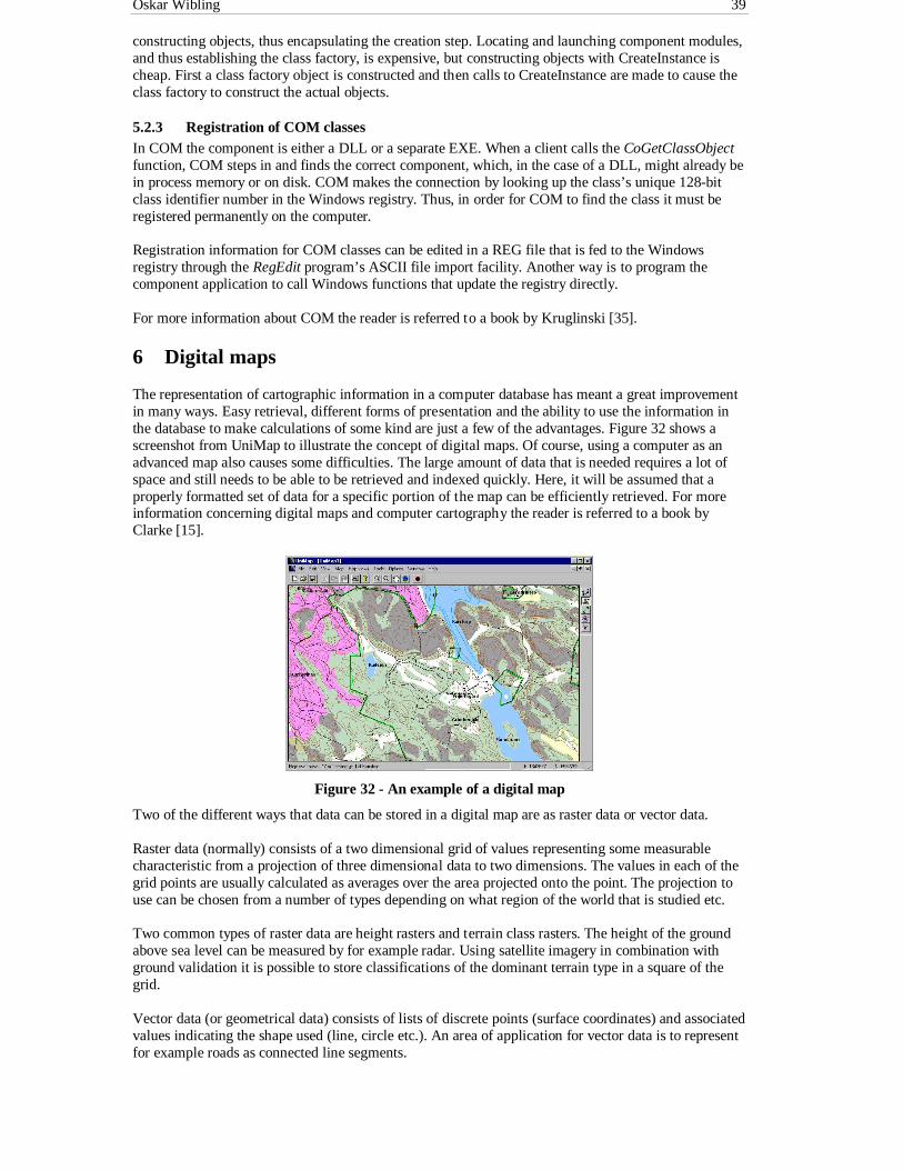
Oskar Wibling 39

constructing objects, thus encapsulating the creation step. Locating and launching component modules,and thus establishing the class factory, is expensive, but constructing objects with CreateInstance ischeap. First a class factory object is constructed and then calls to CreateInstance are made to cause theclass factory to construct the actual objects.

5.2.3 Registration of COM classesIn COM the component is either a DLL or a separate EXE. When a client calls the CoGetClassObjectfunction, COM steps in and finds the correct component, which, in the case of a DLL, might already bein process memory or on disk. COM makes the connection by looking up the class’s unique 128-bitclass identifier number in the Windows registry. Thus, in order for COM to find the class it must beregistered permanently on the computer.

Registration information for COM classes can be edited in a REG file that is fed to the Windowsregistry through the RegEdit program’s ASCII file import facility. Another way is to program thecomponent application to call Windows functions that update the registry directly.

For more information about COM the reader is referred to a book by Kruglinski [35].

6 Digital maps

The representation of cartographic information in a computer database has meant a great improvementin many ways. Easy retrieval, different forms of presentation and the ability to use the information inthe database to make calculations of some kind are just a few of the advantages. Figure 32 shows ascreenshot from UniMap to illustrate the concept of digital maps. Of course, using a computer as anadvanced map also causes some difficulties. The large amount of data that is needed requires a lot ofspace and still needs to be able to be retrieved and indexed quickly. Here, it will be assumed that aproperly formatted set of data for a specific portion of the map can be efficiently retrieved. For moreinformation concerning digital maps and computer cartography the reader is referred to a book byClarke [15].

Figure 32 - An example of a digital map

Two of the different ways that data can be stored in a digital map are as raster data or vector data.

Raster data (normally) consists of a two dimensional grid of values representing some measurablecharacteristic from a projection of three dimensional data to two dimensions. The values in each of thegrid points are usually calculated as averages over the area projected onto the point. The projection touse can be chosen from a number of types depending on what region of the world that is studied etc.

Two common types of raster data are height rasters and terrain class rasters. The height of the groundabove sea level can be measured by for example radar. Using satellite imagery in combination withground validation it is possible to store classifications of the dominant terrain type in a square of thegrid.

Vector data (or geometrical data) consists of lists of discrete points (surface coordinates) and associatedvalues indicating the shape used (line, circle etc.). An area of application for vector data is to representfor example roads as connected line segments.

Oskar Wibling 40

7 MapObjects and GeoPres

7.1 MapObjectsMapObjects is a developing tool produced by ESRI (Environmental Systems Research Institute, Inc.)enabling the developer to embed presentation of geographical data in an application. According toESRI [25] MapObjects consists of an ActiveX Control (OCX) and over thirty programmable ActiveXAutomation Objects that let application developers add dynamic mapping and GIS (GeographicInformation System) capabilities to applications. Since it is built on the Microsoft ActiveX architectureMapObjects can be used with a variety of industry-standard programming environments, such as VisualBasic, Delphi, Visual C++, and others. MapObjects makes it possible to pan and zoom throughmultiple map layers, perform spatial analysis and queries, display data in different ways etc.

7.2 The GeoPres API

GeoPres [41] is a system for presentation of geographical information for the Swedish Armed Forces. Itis an extension of MapObjects to handle defense specific functions that MapObjects alone cannothandle. Examples of such functions are symbol handling and grouping of geographical data for maps.The new components that GeoPres supplies can be divided into four categories: geodictionary, overlay,coordinate transformations, and custom symbols.

The GeoDictionary is a data dictionary over maps available on the system. The overlay is an extensionto the MapObjects tracking layer, which handles information placed on top of the map. Coordinatetransformations manage map projections and geodetic datums, conversion between coordinate systemsand geometric functions. The custom symbols are used for the rendering of the map and of the objectson top of the map.

8 The radio link calculations in MilMap

As mentioned before (see section 1) MilMap is a program developed by Sjöland & Thyselius AB andUniMap is supposed to look as similarly as possible to it but internally use more advanced algorithmsand above all use GeoPres API for the graphical presentation. The radio link calculations used inMilMap will be described here because MilMap is used to compare with the results from the newmodule later.

The model used is a simplified model in which the different attenuation factors are calculated one at atime and then combined to give the total attenuation of the channel. Even though this is a pretty roughapproximation compared to calculating the total attenuation in one step it gives fairly accurate resultsand above all short calculation times.

In MilMap the user can select between using ground radio or radio link. The ground radio selectionpertains to the case in which the antennas are close to the ground so that the ground wave will have tobe taken into account. In the radio link case the assumption is that the stations are elevated considerablyabove the ground so that the ground wave can safely be ignored.

The total attenuation of the channel is calculated using the square-root model and the equation used isthe following (compare with the ones in section 3.10.1):

[dB]FFAAA terraingroundrlstnfreetot 22 +++=

The free space attenuation, Afree, is calculated using the following equations:

Ground radio: [dB]dfFair )(log20)(log200.34 1010 ++=Radio link: [dB]dfFair )(log20)(log202.28 1010 ++=

where f [MHz] is the frequencyd [km] is the distance between the stations

Oskar Wibling 41

Compare this with the formula that was derived in section 3.1.

Arlstn is the total sum of cable damping and antenna gain at both of the stations and is supplied by theuser. It is often negative due to the directional gain of the antennas.

Fground is the propagation factor when modeling the earth as an even plane and is set to zero if radio linkis selected. If ground radio is selected the phase difference between the direct wave and the groundreflected wave is first calculated according to:

d

hh rt

⋅⋅⋅

=∆λ

πφ 4

where ht [m] is the height of the transmitterhr [m] is the height of the receiverλ [m] is the wavelengthd [m] is the distance between the stations

If the phase difference is larger than 0.5 radians the antennas are considered to be elevated enough sothat Fground can be set to zero. If the phase difference is less than or equal to 0.5 radians Fground iscalculated as:

( ) ( ) [dB]hhdF msground log0.20log0.40 1010 ⋅−=

This is a formula that is derived in a similar fashion as the two-wave model described in section 3.2.1.

The knife-edge diffraction propagation factor, Fterrain, is calculated by finding the single height that hasthe largest height inside the first Fresnel zone (compare with the method in section 3.6.1). Themaximum value of (h / r) is noted and used to select the appropriate equation according to:

[dB]r

hF

r

hterrain

8.1

0.407.00.1

−=⇒>

[dB]r

hF

r

hterrain

5.0

0.75.00.15.0

−=⇒≤<

[dB]Fr

hterrain 05.0 =⇒≤

This is an even simpler approximation to the single knife-edge propagation factor than the one by Leethat was described in section 3.3.

9 The new terrain analysis module

This chapter mainly covers algorithms and underlying concepts used in the new terrain analysismodule. For a more detailed description (in Swedish) of the tools and pictures of how the developedsystem looks the reader is referred to Appendix B.

9.1 Structure of the databases used

The data needed in the terrain analysis module is height and terrain data for Sweden. Since the GeoPresAPI does not (yet) contain functionality for retrieving these data another approach had to be taken. Thesolution was to use functions from two MilMap DLLs (mmdb32.dll and mm2_32.dll) and part of theMilMap database to get the data that was needed.

The MilMap databases cover all of Sweden and contain both height and terrain type information. Theheight database has a grid spacing of 50 meters and a vertical resolution of one meter. The terraindatabase uses thirteen different terrain type classes (water, open land etc.) that have been extracted byclassifying satellite photographs. In larger cities an additional six terrain classes are used for different

Oskar Wibling 42

urban types. The terrain database used can be selected between a larger one having a grid spacing of 25meters and a smaller one having a grid spacing of 50 meters.

Issuing the command MM_GetHeight(…) in the MilMap DLLs returns the height of the lower leftmostgridpoint in the square grid surrounding the given point (See Figure 33). It could lead to a greatimprovement in the results if instead some kind of interpolating method was used to find the height in acertain position. For example a weighed sum of the heights in the four nearest points.

Figure 33 – Height selecting in the MilMap database

Issuing the command MM_GetClass (…) in the MilMap DLLs returns the terrain class of the lowerleftmost gridpoint in the square grid surrounding the given point (See Figure 33). Here the accuracycould also be improved if the terrain class of the nearest point was instead returned.

The initial approach taken was to buffer all the height and terrain data needed for a calculation and thenperform the calculation on the buffered data. This was done to save database accesses and thus time.However, it proved to be less desirable to allocate large amounts of memory than to use the little extratime needed to access the database. The underlying MilMap database handler is also programmed tobuffer data in the near vicinity of a requested point to speed up accesses.

9.2 The radio link calculation method in the module

The prediction of the signal attenuation is done using the square-root model with possible additions ofother contributions as described in section 3.10.1, i.e.:

[dB]FFAAA ndiffractiosmoothrlstnfreetotal FFF atmosphereurbanvegetation22 ++++++=

where Afree is the attenuation in free spaceArlstn is the total sum of cable damping and antenna gain at both of the stationsFsmooth is the propagation factor calculated for a smooth, spherical earth modelAdiffraction is the propagation factor calculated for a knife-edge diffraction modelFvegetation is additional attenuation due to vegetationFurban is additional attenuation due to buildingsFatmosphere is additional attenuation due to atmospheric gases

This model was chosen both because of its simplicity (which leads to fast calculation times) andbecause of its widespread use.

For calculating the free space attenuation the following expression, which was derived in section 3.1, isused:

( ) ( ) [dB]fdAfree log20log2045.32 1010 ++=

The total sum of cable damping and antenna gain is supplied by the user and is as mentioned beforeoften negative since the antenna gain is usually greater than the cable damping which leads to anamplification of the signal, i.e. a negative attenuation.

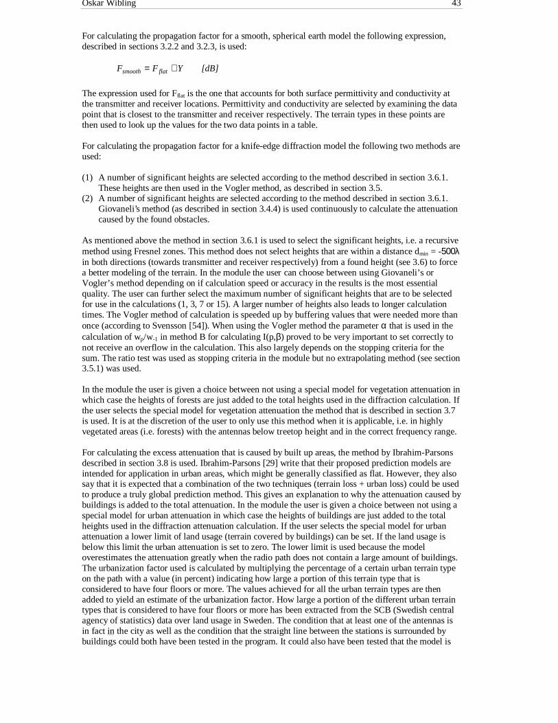
Oskar Wibling 43

For calculating the propagation factor for a smooth, spherical earth model the following expression,described in sections 3.2.2 and 3.2.3, is used:

[dB]YFF flatsmooth +=

The expression used for Fflat is the one that accounts for both surface permittivity and conductivity atthe transmitter and receiver locations. Permittivity and conductivity are selected by examining the datapoint that is closest to the transmitter and receiver respectively. The terrain types in these points arethen used to look up the values for the two data points in a table.

For calculating the propagation factor for a knife-edge diffraction model the following two methods areused:

(1) A number of significant heights are selected according to the method described in section 3.6.1.These heights are then used in the Vogler method, as described in section 3.5.

(2) A number of significant heights are selected according to the method described in section 3.6.1.Giovaneli’s method (as described in section 3.4.4) is used continuously to calculate the attenuationcaused by the found obstacles.

As mentioned above the method in section 3.6.1 is used to select the significant heights, i.e. a recursivemethod using Fresnel zones. This method does not select heights that are within a distance dmin = -500λin both directions (towards transmitter and receiver respectively) from a found height (see 3.6) to forcea better modeling of the terrain. In the module the user can choose between using Giovaneli’s orVogler’s method depending on if calculation speed or accuracy in the results is the most essentialquality. The user can further select the maximum number of significant heights that are to be selectedfor use in the calculations (1, 3, 7 or 15). A larger number of heights also leads to longer calculationtimes. The Vogler method of calculation is speeded up by buffering values that were needed more thanonce (according to Svensson [54]). When using the Vogler method the parameter α that is used in thecalculation of wp/w-1 in method B for calculating I(p,β) proved to be very important to set correctly tonot receive an overflow in the calculation. This also largely depends on the stopping criteria for thesum. The ratio test was used as stopping criteria in the module but no extrapolating method (see section3.5.1) was used.

In the module the user is given a choice between not using a special model for vegetation attenuation inwhich case the heights of forests are just added to the total heights used in the diffraction calculation. Ifthe user selects the special model for vegetation attenuation the method that is described in section 3.7is used. It is at the discretion of the user to only use this method when it is applicable, i.e. in highlyvegetated areas (i.e. forests) with the antennas below treetop height and in the correct frequency range.

For calculating the excess attenuation that is caused by built up areas, the method by Ibrahim-Parsonsdescribed in section 3.8 is used. Ibrahim-Parsons [29] write that their proposed prediction models areintended for application in urban areas, which might be generally classified as flat. However, they alsosay that it is expected that a combination of the two techniques (terrain loss + urban loss) could be usedto produce a truly global prediction method. This gives an explanation to why the attenuation caused bybuildings is added to the total attenuation. In the module the user is given a choice between not using aspecial model for urban attenuation in which case the heights of buildings are just added to the totalheights used in the diffraction attenuation calculation. If the user selects the special model for urbanattenuation a lower limit of land usage (terrain covered by buildings) can be set. If the land usage isbelow this limit the urban attenuation is set to zero. The lower limit is used because the modeloverestimates the attenuation greatly when the radio path does not contain a large amount of buildings.The urbanization factor used is calculated by multiplying the percentage of a certain urban terrain typeon the path with a value (in percent) indicating how large a portion of this terrain type that isconsidered to have four floors or more. The values achieved for all the urban terrain types are thenadded to yield an estimate of the urbanization factor. How large a portion of the different urban terraintypes that is considered to have four floors or more has been extracted from the SCB (Swedish centralagency of statistics) data over land usage in Sweden. The condition that at least one of the antennas isin fact in the city as well as the condition that the straight line between the stations is surrounded bybuildings could both have been tested in the program. It could also have been tested that the model is

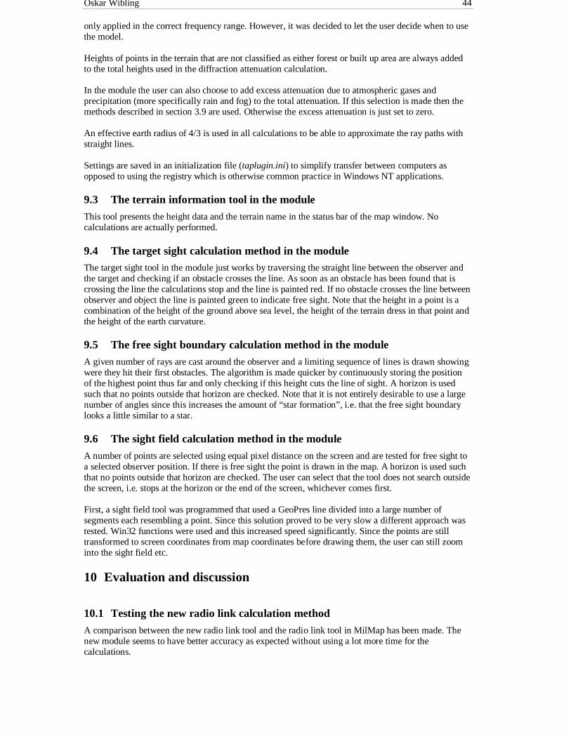
Oskar Wibling 44

only applied in the correct frequency range. However, it was decided to let the user decide when to usethe model.

Heights of points in the terrain that are not classified as either forest or built up area are always addedto the total heights used in the diffraction attenuation calculation.

In the module the user can also choose to add excess attenuation due to atmospheric gases andprecipitation (more specifically rain and fog) to the total attenuation. If this selection is made then themethods described in section 3.9 are used. Otherwise the excess attenuation is just set to zero.

An effective earth radius of 4/3 is used in all calculations to be able to approximate the ray paths withstraight lines.

Settings are saved in an initialization file (taplugin.ini) to simplify transfer between computers asopposed to using the registry which is otherwise common practice in Windows NT applications.

9.3 The terrain information tool in the module

This tool presents the height data and the terrain name in the status bar of the map window. Nocalculations are actually performed.

9.4 The target sight calculation method in the moduleThe target sight tool in the module just works by traversing the straight line between the observer andthe target and checking if an obstacle crosses the line. As soon as an obstacle has been found that iscrossing the line the calculations stop and the line is painted red. If no obstacle crosses the line betweenobserver and object the line is painted green to indicate free sight. Note that the height in a point is acombination of the height of the ground above sea level, the height of the terrain dress in that point andthe height of the earth curvature.

9.5 The free sight boundary calculation method in the module

A given number of rays are cast around the observer and a limiting sequence of lines is drawn showingwere they hit their first obstacles. The algorithm is made quicker by continuously storing the positionof the highest point thus far and only checking if this height cuts the line of sight. A horizon is usedsuch that no points outside that horizon are checked. Note that it is not entirely desirable to use a largenumber of angles since this increases the amount of “star formation”, i.e. that the free sight boundarylooks a little similar to a star.

9.6 The sight field calculation method in the module

A number of points are selected using equal pixel distance on the screen and are tested for free sight toa selected observer position. If there is free sight the point is drawn in the map. A horizon is used suchthat no points outside that horizon are checked. The user can select that the tool does not search outsidethe screen, i.e. stops at the horizon or the end of the screen, whichever comes first.

First, a sight field tool was programmed that used a GeoPres line divided into a large number ofsegments each resembling a point. Since this solution proved to be very slow a different approach wastested. Win32 functions were used and this increased speed significantly. Since the points are stilltransformed to screen coordinates from map coordinates before drawing them, the user can still zoominto the sight field etc.

10 Evaluation and discussion

10.1 Testing the new radio link calculation method

A comparison between the new radio link tool and the radio link tool in MilMap has been made. Thenew module seems to have better accuracy as expected without using a lot more time for thecalculations.

Oskar Wibling 45

A problem when comparing the radio link calculation methods was the lack of a sufficient amount ofreal measurement data. The four test paths that were available are shown in Figure 34 - Figure 37. Thefrequency used was 1.6 GHz and the polarization was horizontal.

Figure 34 – Test path 1

Figure 35 – Test path 2

Figure 36 – Test path 3

Figure 37 – Test path 4

The comparisons were made by calculating the predicted attenuation using the two MilMap radio linkmethods and then by using the new radio link tool. The new tool was set to use first the Giovanelimethod with a maximum of 3 heights and then the Vogler method with a maximum of 3 heights.Vegetation and buildings were handled by adding their height to the total height. No atmosphericexcess attenuation was calculated. The terrain types used in MilMap and UniMap respectively weregiven the same mean heights. All other common settings in the modules were set to the same values.The results of the comparison can be seen in Table 2.

Path Measuredattenuation [dB]

MilMap, radiolink [dB]

MilMap, groundradio [dB]

UniMap, Giovaneli,max 3 heights [dB]

UniMap, Vogler,max 3 heights [dB]

1 146 117 123 120.51 142.12 136 125 130 131.17 150.423 151 124 130 134.46 153.344 146 131 137 144.54 167.28

Table 2 - Comparison between the old and new radio link calculations

Figure 38 shows a diagram of the measurement data.

Oskar Wibling 46

Figure 38 – Comparison between the old and new radio link calculations

To clarify the results the deviations from the measured values have been calculated. The mean valuesof these deviations have then been calculated. See Table 3 for these values.

Path MilMap, radiolink [dB]

MilMap, groundradio [dB]

UniMap, Giovaneli,max 3 heights [dB]

UniMap, Vogler,max 3 heights [dB]

1 29 23 25.49 3.92 11 6 4.83 14.423 27 21 16.54 2.344 15 9 1.46 21.28Mean 20.5 14.75 12.08 10.49

Table 3 - Deviations from the measured values

Even though the measurements are too few too draw any statistically valid conclusions it can still besuspected that an improvement has been made. A problem is that a significant part of the error is due tolack of exact terrain data in the form of real forest heights etc., especially near the stations.

10.2 Error sources in the radio link toolSome of the error sources in the new radio link tool are the following:

• Obstacles in the near vicinity of the stations is the single largest source of error in radio linkcalculations.

• Quantification of both the height and terrain class data. Classifying the terrain data too roughlyconcerning height, relative permittivity and conductivity.

• The square-root model is known to quite often overestimate the path loss.• All the approximations made in the calculations.

10.3 The other new terrain analysis tools

The other tools in the new module are very similar to the old ones in MilMap. How the new tools looklike and what settings that can be made for them can all be read in the user’s manual in Appendix B.

11 Future work

It might be a good idea to add a check similar to the one in MilMap to see if the grazing angle is largeenough to set the even, spherical earth attenuation to zero. Since the model currently used in theprogram does not give correct results when using very high antennas this could be an acceptablesolution.

Since a symbol manager has not yet been produced for UniMap the moving of radio link endpoints etc.has not been implemented the correct way. As it works now, a routine goes through all the radio linkdialogs and asks them if they want to move one of their positions when a left button mouse click has

Oskar Wibling 47

been detected. This can be very time consuming if there are many radio link dialogs on the screen. Theway it is supposed to work is that when the main application sees that a symbol has been moved itsends a move-message to for example the radio link plugin containing the identifier of the symbol.

Something could be done with the numerical precision. Doubles are now used in most parts of theprogram. If long doubles or long floats were used the numerical precision could be enhanced. However,the built in errors in using simplified models is probably so large that not much would be gained.

It has been shown that in some cases the Vogler method for calculating diffraction attenuationconverges faster if the terrain is turned upside down. Especially on some paths where slow convergenceis normally achieved (paths that have very little height variation, for example over open sea) this couldbe implemented as to decrease calculation times.

It would be interesting to explore the new three dimensional attenuation prediction methods. If a largeamount of real measurement data was available it would also be interesting to see if a neural networkcould be trained to predict the attenuation accurately.

12 Acknowledgements

The author wishes to thank the following people (ordered by last name) for their participation inrealizing this thesis:

Eva B. Björck, Försvarets Forskningsanstalt (FOA), Biblioteket i LinköpingRichard Elg, Sjöland & Thyselius ABEmil Gustafsson, Sjöland & Thyselius ABJonas Jerfsten, Sjöland & Thyselius ABPeter Krans, Stab SbS, Swedish Armed Forces, EnköpingLars Ladell, Celsius FFV AerotechRichard Mohringe, Sjöland & Thyselius ABFaron Moller, Computing Science Department (CSD), Uppsala UniversityMagnus Sjöland, Sjöland & Thyselius ABRune Thyselius, Sjöland & Thyselius ABTommy Öberg, Signals and Systems Group, Uppsala UniversityThe staff at KTHB, Stockholm and the Beurling library, Uppsala

13 References

[1] Ahlin L, Zander J, Principles of wireless communications, Studentlitteratur, Lund, Sweden, 1998

[2] Allsebrook K, Parsons J D, Mobile Radio Propagation in British Cities at Frequencies in the VHFand UHF Bands, IEEE Trans. Veh. Technol., vol. VT-26, no. 4, pp. 313-323, Nov 1977

[3] Altshuler E A, A Simple Expression for Estimating Attenuation by Fog at Millimeter Wavelengths,IEEE Trans. Ant. Prop., vol. AP-32, no. 7, pp. 757-758

[4] Altshuler E A, Addendum to A Simple Expression for Estimating Attenuation by Fog at MillimeterWavelengths, IEEE Trans. Ant. Prop., vol. AP-34, no. 8, pp. 1067

[5] Anderson L J, Trolese L G, Simplified Method for Computing Knife-Edge Diffraction in theShadow Region, IEEE Trans. Anten. Prop., pp. 281-286, July 1958

[6] Asp B, Eriksson G, Holm P, Detvag-90 – Final report, FOA report R--97-00566-504, FörsvaretsForskningsanstalt, Linköping, Sweden, Sept 1997

[7] Asp B, Bröms M, Introduktion till vågutbredning, FOA report R--94-00014-3.5--SE, FörsvaretsForskningsanstalt, Linköping, Sweden, May 1995

[8] Bullington K, Radio Propagation at Frequencies Above 30 Megacycles, Proc. of the I.R.E., vol.35, pp.1122-1136, Oct 1947

Oskar Wibling 48

[9] Bullington K, Radio Propagation for Vehicular Communications, IEEE Trans. Veh. Technol., vol.VT-26, no. 4, Nov 1977

[10] Blomquist Å, Local Ground Wave Field Strength Variations in the Frequency Range 30-1000MHz, International Conference on Electromagnetic Wave Propagation, Liège, ElectromagneticWave Propagation, Editor: Desirant M, Michiels J L, Academic Press, pp. 127-142, 1958

[11] Blomquist Å, Markvågsmodell för VHF-området vid sfärisk jordyta, FOA 3 report A 3763-E2,Försvarets Forskningsanstalt, Stockholm, Sweden, June 1973

[12] Blomquist Å, Ladell L, Prediction and Calculation of Transmission Loss in Different Types ofTerrain, FOA 3 report C 3792-E2, Försvarets Forskningsanstalt, Stockholm, Sweden, June 1974

[13] Blomquist Å et al, Radiovågors Utbredning - Jordytans Inverkan, FOA Compendium 24A, ch. 5-6, 1969

[14] Chamberlin K A, Luebbers R J, An Evaluation of Longley-Rice and GTD Propagation Models,IEEE Trans. Ant. Prop., vol. AP-30, no. 6, pp. 1093-1098, Nov 1982

[15] Clarke K C, Analytical and Computer Cartography, Prentice Hall, Englewood Cliffs, New Jersey,1990

[16] Delahoy M, Whitfield D, Performance and Design of Small Satellite Earth Stations,Communications Laboratory Report 95/10, 1995

[17] Dence D, Tamir T, Radio loss of lateral waves in forest environments, Radio Science, vol. 4, no. 4,pp. 307-318, April 1969

[18] Deygout J, Multiple Knife-Edge Diffraction of Microwaves, IEEE Trans. Ant. Prop., vol. AP-14,no. 4, pp. 480-489, July 1966

[19] Durkin J, Computer Prediction of Service Areas for VHF and UHF Land Mobile Radio Services,IEEE Trans. Veh. Technol., vol. VT-26, no. 4, pp. 323-327, Nov 1977

[20] Eklund F, Nilsson L, Metod för beräkning av diffraktionsdämpning över en serie kniveggar, FOAreport A 3687-61, Försvarets Forskningsanstalt, Stockholm, Sweden, Feb 1967

[21] Ekström C, Windowsimplementering av vågutbredningsmodell, FOA report C 30767-3.6,Försvarets Forskningsanstalt, Linköping, Sweden, June 1994

[22] Epstein J, Peterson D W, An Experimental Study of Wave Propagation at 850 MC, Proc. of theI.R.E., vol. 41, pp. 595-611, May 1953

[23] Eriksson G, DETVAG-90, A pilot study of extended frequency range for the ground-wavepropagation model Detvag, FOA report C 30655-3.5, Försvarets Forskningsanstalt, Linköping,Sweden, May 1992

[24] Eriksson G, Wave-propagation aspects on VHF-radar applications, FOA report C 30754-3.5,Försvarets Forskningsanstalt, Linköping, Sweden, March 1994

[25] ESRI, MapObjects Embeddable GIS and Mapping Components for Application Developers,Environmental Systems Research Institute Inc., 1998

[26] Giovaneli C L, An Analysis of Simplified Solutions for Multiple Knife-Edge Diffraction, IEEETrans. Ant. Prop., vol. AP-32, no. 3, pp. 297-301, March 1984

[27] Holm P, DETVAG-90, Use of GTD for wave propagation over earth, FOA report R--94-00003-3.5, Försvarets Forskningsanstalt, Linköping, Sweden, Dec 1994

Oskar Wibling 49

[28] Holm P, DETVAG-90, Use of the ground-wave program GRWAVE in the wave-propagation modelDETVAG, FOA report C 30678-3.5, Försvarets Forskningsanstalt, Linköping, Sweden, Feb 1993

[29] Ibrahim M F, Parsons J D, Signal strength prediction in built-up areas Part 1: Median signalstrength, IEE Proc., vol. 130, part F, no. 5, pp. 377-384, Aug 1983

[30] Ippolito L J, Propagation Effects Handbook for Satellite Systems Design – A Summary ofPropagation Impairments on 10-100 GHz Satellite Links With Techniques for System Design,Fourth Edition, NASA Reference Publication 1082(04), Westinghouse Electric Corporation,Baltimore, Maryland, USA, 1989

[31] ITU-R Report 1145, Propagation over irregular terrain with and without vegetation

[32] Jakes W C, Microwave Mobile Communications, Wiley, New York, 1974

[33] Keller J B, Geometrical Theory of Diffraction, Journal of the Optical Society of America, vol. 52,no. 2, pp. 116-130, Feb 1962

[34] Kouyoumjian R G, A Uniform Geometrical Theory of Diffraction for an Edge in a PerfectlyConducting Surface, Proc. of the IEEE, vol. 62, no. 11, pp. 1448-1461, Nov 1974

[35] Kruglinski D J, Inside Visual C++, Fourth Edition, Microsoft Press, Redmond, Washington, USA,1997

[36] Ladell L, Terrängens inverkan på sambandsmöjligheterna inom VHF-området. Jämförelse mellanolika beräkningsmetoder, FOA 3 report A 3768-E2, Försvarets Forskningsanstalt, Stockholm,Sweden, Nov 1973

[37] Ladell L, Transmission loss predictions in wooded terrain, FOA report B 30096-3.3, FörsvaretsForskningsanstalt, Linköping, Sweden, Sep 1986

[38] Lebherz M, Wiesbeck W, Krank W, A Versatile Wave Propagation Model for the VHF/UHFRange Considering Three-Dimensional Terrain, IEEE Trans. Ant. Prop., vol. 40, no. 10, pp. 1121-1131, Oct 1992

[39] Lee W C Y, Mobile communications engineering, Second Edition, McGraw-Hill Series onTelecommunications, 1997

[40] Luebbers R J, Propagation Prediction for Hilly Terrain Using GTD Wedge Diffraction, IEEETrans. Ant. Prop., vol. AP-32, no. 9, pp. 951-955, Sep 1984

[41] Lundberg J, Technical And Information Aspects on GeoPres, ESRI User Conference, 1998

[42] Millington G, Ground-wave propagation over an inhomogenous smooth earth, Proc. IEE, vol. 96,pp. 53-64, 1949.

[43] Nilsson S, Yttäckande radionät, mätning och prediktion av transmissionsförlust vid 400 och 900MHz, FOA report C 30457-3.3, Försvarets Forskningsanstalt, Linköping, Sweden, Oct 1987

[44] Norton K A, The Calculation of Ground-Wave Field Intensity Over a Finitely ConductingSpherical Earth, Proc. of the I.R.E., vol. 29, pp. 623, Dec 1941

[45] Olsen R L, Rogers D V, Hedge D B, The aRb Relation in the Calculation of Rain Attenuation,IEEE Trans. Ant. Prop., vol. AP-26, pp. 318-329, 1978

[46] Ott R H, Berry L A, An alternative integral equation for propagation over irregular terrain, RadioScience, vol. 5, no. 5, pp. 767-771, May 1970

[47] Ott R H, An alternative integral equation for propagation over irregular terrain, 2, Radio Science,vol. 6, no. 4, pp. 429-435, April 1971

Oskar Wibling 50

[48] Parsons D, The mobile radio propagation channel, Pentech Press, London, 1991

[49] Pogorzelski R J, A note on some common diffraction link loss models, Radio Science, vol. 17, no.6, pp. 1536-1540, Nov-Dec 1982

[50] Press W H, Flannery B P, Teukolsky S A, Vetterling W T, Numerical Recipes, The Art ofScientific Computing (Fortran Version), Press Syndicate of the University of Cambridge,Cambridge, 1989

[51] Rotheram S, Ground-wave propagation Part 1: Theory for short distances, IEE Proc., vol. 128,part F, no. 5, pp. 275-295, Oct 1981

[52] Råde L, Westergren B, Beta, Mathematics Handbook, Second Edition, Studenlitteratur, Lund,1990

[53] Stokke K N, Some graphical considerations on Millington’s method for calculating field strengthover inhomogeneous earth, Telecommunications Journal, vol. 42, pp. 157-163, 1975

[54] Svensson I, DETVAG-90 An Implementation of Vogler’s method for calculation of multiple knife-edge diffraction, FOA report C 30743-3.5, Försvarets Forskningsanstalt, Linköping, Sweden, June1994

[55] Tamir T, On Radio-Wave Propagation in Forest Environments, IEEE Trans. Ant. Prop., vol. AP-15, no. 6, pp. 806-817, Nov 1967

[56] Tamir T, Radio Wave Propagation Along Mixed Paths in Forest Environments, IEEE Trans. Ant.Prop., vol. AP-25, no. 4, pp.471-477, July 1977

[57] Vogler L E, An attenuation function for multiple knife-edge diffraction, Radio Science, vol. 17, no.6, pp. 1541-1546, Nov-Dec 1982

[58] Whitteker J H, A series solution for diffraction over terrain modeled as multiple bridged knife-edges, Radio Science, vol. 28, no. 4, pp. 487-500, July-Aug 1993

[59] Öberg T, Modulation, detektion och kodning, Second Edition, Uppsala Universitet Repro HSC,Uppsala, Sweden, 1997

51

Appendix

A Relative permittivity and conductivity constants

The following table contains the electrical characteristics for a few different terrain types. The valueshave been taken from tables in the references [1] and [39]. They have been used when setting thedefault values for the terrain types in the developed module.

Type of surface Relative permittivity, εr Conductivity, σ [S/m]Bare, dry, sandy loam 2 0.03Turf with short, dry grass 3 0.05Urban ground 3 0.0001Dry ground 4 0.001Turf with short, wet grass 6 0.1Rocky terrain 7 0.005Rural ground 14 0.01Typical ground 15 0.005Bare, sandy loam saturated with water 24 0.6Wet ground 30 0.02Fresh water 80 0.005Sea water 80 4

Table A1 – Some relative permittivity and conductivity constants

B User’s manual for the developed system (in Swedish)

B.1 Uppstart av systemet

Viktigt att tänka på då DLL:en för terränganalys används är att både filerna ”milmap.ini” och”taplugin.ini” ligger i samma katalog som ”TAPlugin.dll”. Då man startat upp systemet ochterränganalysmodulen är installerad så får man en bild liknande den i figur 1. Terränganalysverktygensknappar syns uppe till höger i figuren.

Figur 1 – Systemet efter uppstart

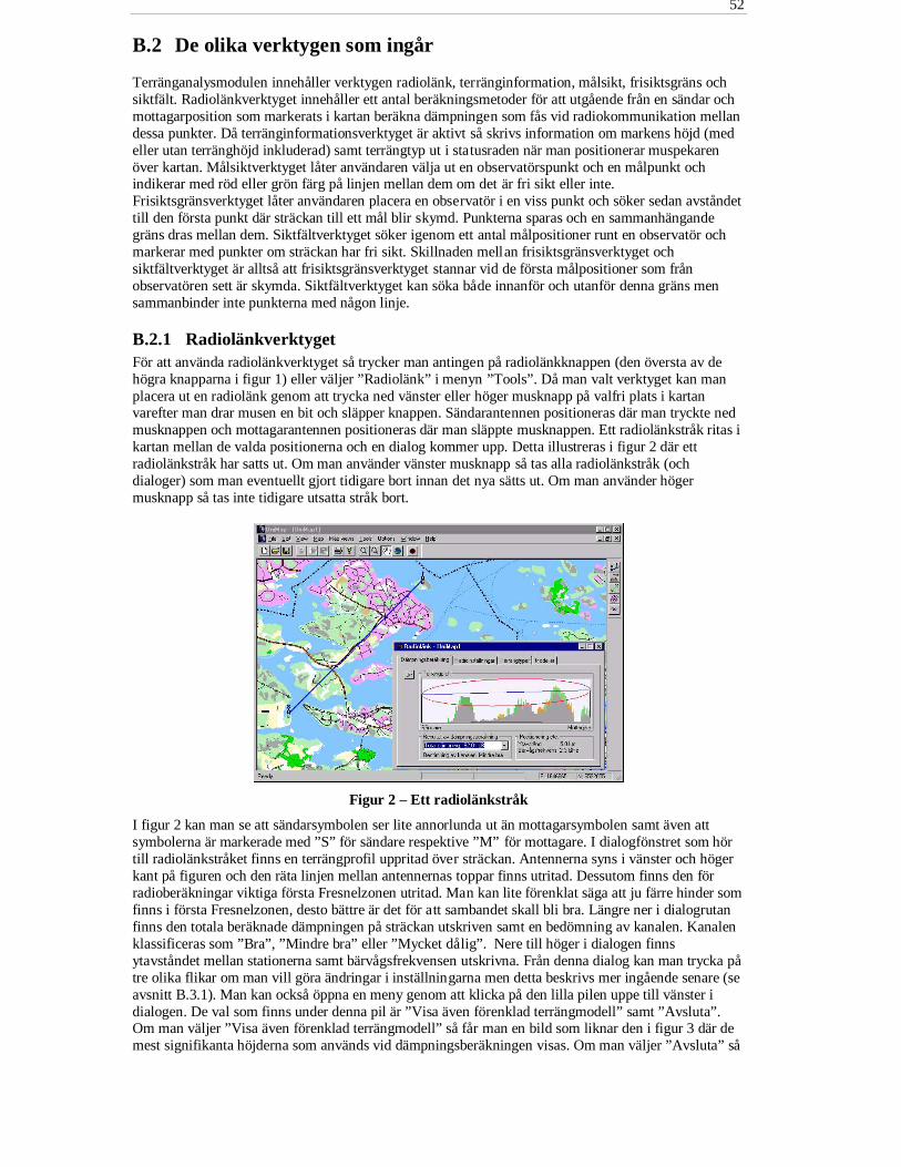
52

B.2 De olika verktygen som ingår

Terränganalysmodulen innehåller verktygen radiolänk, terränginformation, målsikt, frisiktsgräns ochsiktfält. Radiolänkverktyget innehåller ett antal beräkningsmetoder för att utgående från en sändar ochmottagarposition som markerats i kartan beräkna dämpningen som fås vid radiokommunikation mellandessa punkter. Då terränginformationsverktyget är aktivt så skrivs information om markens höjd (medeller utan terränghöjd inkluderad) samt terrängtyp ut i statusraden när man positionerar muspekarenöver kartan. Målsiktverktyget låter användaren välja ut en observatörspunkt och en målpunkt ochindikerar med röd eller grön färg på linjen mellan dem om det är fri sikt eller inte.Frisiktsgränsverktyget låter användaren placera en observatör i en viss punkt och söker sedan avståndettill den första punkt där sträckan till ett mål blir skymd. Punkterna sparas och en sammanhängandegräns dras mellan dem. Siktfältverktyget söker igenom ett antal målpositioner runt en observatör ochmarkerar med punkter om sträckan har fri sikt. Skillnaden mellan frisiktsgränsverktyget ochsiktfältverktyget är alltså att frisiktsgränsverktyget stannar vid de första målpositioner som frånobservatören sett är skymda. Siktfältverktyget kan söka både innanför och utanför denna gräns mensammanbinder inte punkterna med någon linje.

B.2.1 RadiolänkverktygetFör att använda radiolänkverktyget så trycker man antingen på radiolänkknappen (den översta av dehögra knapparna i figur 1) eller väljer ”Radiolänk” i menyn ”Tools”. Då man valt verktyget kan manplacera ut en radiolänk genom att trycka ned vänster eller höger musknapp på valfri plats i kartanvarefter man drar musen en bit och släpper knappen. Sändarantennen positioneras där man tryckte nedmusknappen och mottagarantennen positioneras där man släppte musknappen. Ett radiolänkstråk ritas ikartan mellan de valda positionerna och en dialog kommer upp. Detta illustreras i figur 2 där ettradiolänkstråk har satts ut. Om man använder vänster musknapp så tas alla radiolänkstråk (ochdialoger) som man eventuellt gjort tidigare bort innan det nya sätts ut. Om man använder högermusknapp så tas inte tidigare utsatta stråk bort.

Figur 2 – Ett radiolänkstråk

I figur 2 kan man se att sändarsymbolen ser lite annorlunda ut än mottagarsymbolen samt även attsymbolerna är markerade med ”S” för sändare respektive ”M” för mottagare. I dialogfönstret som hörtill radiolänkstråket finns en terrängprofil uppritad över sträckan. Antennerna syns i vänster och högerkant på figuren och den räta linjen mellan antennernas toppar finns utritad. Dessutom finns den förradioberäkningar viktiga första Fresnelzonen utritad. Man kan lite förenklat säga att ju färre hinder somfinns i första Fresnelzonen, desto bättre är det för att sambandet skall bli bra. Längre ner i dialogrutanfinns den totala beräknade dämpningen på sträckan utskriven samt en bedömning av kanalen. Kanalenklassificeras som ”Bra”, ”Mindre bra” eller ”Mycket dålig”. Nere till höger i dialogen finnsytavståndet mellan stationerna samt bärvågsfrekvensen utskrivna. Från denna dialog kan man trycka påtre olika flikar om man vill göra ändringar i inställningarna men detta beskrivs mer ingående senare (seavsnitt B.3.1). Man kan också öppna en meny genom att klicka på den lilla pilen uppe till vänster idialogen. De val som finns under denna pil är ”Visa även förenklad terrängmodell” samt ”Avsluta”.Om man väljer ”Visa även förenklad terrängmodell” så får man en bild som liknar den i figur 3 där demest signifikanta höjderna som används vid dämpningsberäkningen visas. Om man väljer ”Avsluta” så

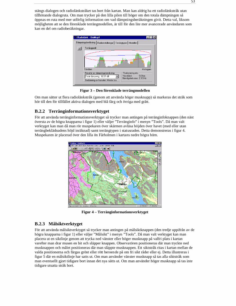
53

stängs dialogen och radiolänkstråket tas bort från kartan. Man kan aldrig ha ett radiolänkstråk utantillhörande dialogruta. Om man trycker på den lilla pilen till höger om den totala dämpningen såöppnas en ruta med mer utförlig information om vad dämpningsberäkningen givit. Detta val, liksommöjligheten att se den förenklade terrängmodellen, är till för den lite mer avancerade användaren somkan en del om radioberäkningar.

Figur 3 – Den förenklade terrängmodellen

Om man sätter ut flera radiolänkstråk (genom att använda höger musknapp) så markeras det stråk somhör till den för tillfället aktiva dialogen med blå färg och övriga med grått.

B.2.2 TerränginformationsverktygetFör att använda terränginformationsverktyget så trycker man antingen på terränginfoknappen (den nästöversta av de högra knapparna i figur 1) eller väljer ”Terränginfo” i menyn ”Tools”. Då man valtverktyget kan man då man rör muspekaren över skärmen avläsa höjden över havet (med eller utanterrängbeklädnadens höjd inräknad) samt terrängtypen i statusraden. Detta demonstreras i figur 4.Muspekaren är placerad över den lilla ön Fårholmen i kartans nedre högra hörn.

Figur 4 – Terränginformationsverktyget

B.2.3 MålsiktverktygetFör att använda målsiktverktyget så trycker man antingen på målsiktknappen (den tredje uppifrån av dehögra knapparna i figur 1) eller väljer ”Målsikt” i menyn ”Tools”. Då man valt verktyget kan manplacera ut en siktlinje genom att trycka ned vänster eller höger musknapp på valfri plats i kartanvarefter man drar musen en bit och släpper knappen. Observatören positioneras där man tryckte nedmusknappen och målet positioneras där man släppte musknappen. Ett siktstråk ritas i kartan mellan devalda positionerna och färgas grönt eller rött beroende på om fri sikt råder eller ej. Detta illustreras ifigur 5 där en målsiktlinje har satts ut. Om man använder vänster musknapp så tas alla siktstråk somman eventuellt gjort tidigare bort innan det nya sätts ut. Om man använder höger musknapp så tas intetidigare utsatta stråk bort.

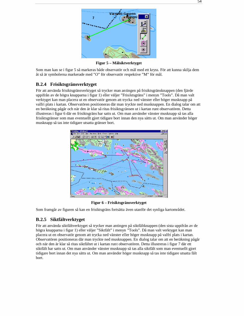
54

Figur 5 – Målsiktverktyget

Som man kan se i figur 5 så markeras både observatör och mål med ett kryss. För att kunna skilja demåt så är symbolerna markerade med ”O” för observatör respektive ”M” för mål.

B.2.4 FrisiktsgränsverktygetFör att använda frisiktsgränsverktyget så trycker man antingen på frisiktsgränsknappen (den fjärdeuppifrån av de högra knapparna i figur 1) eller väljer ”Frisiktsgräns” i menyn ”Tools”. Då man valtverktyget kan man placera ut en observatör genom att trycka ned vänster eller höger musknapp påvalfri plats i kartan. Observatören positioneras där man tryckte ned musknappen. En dialog talar om atten beräkning pågår och när den är klar så ritas frisiktsgränsen ut i kartan runt observatören. Dettaillustreras i figur 6 där en frisiktsgräns har satts ut. Om man använder vänster musknapp så tas allafrisiktsgränser som man eventuellt gjort tidigare bort innan den nya sätts ut. Om man använder högermusknapp så tas inte tidigare utsatta gränser bort.

Figur 6 – Frisiktsgränsverktyget

Som framgår av figuren så kan en frisiktsgräns fortsätta även utanför det synliga kartområdet.

B.2.5 SiktfältverktygetFör att använda siktfältverktyget så trycker man antingen på siktfältknappen (den sista uppifrån av dehögra knapparna i figur 1) eller väljer ”Siktfält” i menyn ”Tools”. Då man valt verktyget kan manplacera ut en observatör genom att trycka ned vänster eller höger musknapp på valfri plats i kartan.Observatören positioneras där man tryckte ned musknappen. En dialog talar om att en beräkning pågåroch när den är klar så ritas siktfältet ut i kartan runt observatören. Detta illustreras i figur 7 där ettsiktfält har satts ut. Om man använder vänster musknapp så tas alla siktfält som man eventuellt gjorttidigare bort innan det nya sätts ut. Om man använder höger musknapp så tas inte tidigare utsatta fältbort.

55

Figur 7 – Siktfältverktyget

Även siktfält kan fortsätta utanför den synliga kartytan, men det går att förhindra genom att ändra eninställning (se avsnitt B.3.2.4). Detta kan vara en fördel eftersom det ibland tar lång tid att beräknasiktfält.

B.3 Inställningar

B.3.1 Inställningar i radiolänkverktygetUnder de olika flikarna i dialogen som hör till ett radiolänkstråk finns möjlighet att göra en radinställningar.

En flik har rubriken ”Radioinställningar” och där kan inställningar som har med radioutrustningens typoch antennernas positioner göras. Se figur 8 för en illustration av detta.

Figur 8 – Radioinställningar i radiolänkdialog

Olika radioutrustningar kan väljas under fliken ”Utrustning” uppe till vänster. Positioner för sändar ochmottagarantenner kan antingen knappas in manuellt i rutorna nere till höger eller flyttas i kartan genomatt först trycka på ”Peka”-knappen för antingen sändare eller mottagare och sedan klicka i kartan medvänster musknapp på den plats där man vill placera den berörda antennen. Observera att det bara går att”peka” i kartan för en av ändpunkterna i taget. Det går dock utmärkt att om man har fleraradiolänkstråk i kartan trycka på ”Peka”-knappen i två olika radiolänkdialoger och sedan peka i kartan.Båda de berörda antennerna flyttas då till den positionen. Detta är praktiskt om man vill ha fleraradiolänkstråk efter varandra i en serie, d.v.s. segmenterade radiolänkar. Då man tryckt på en av”Peka”-knapparna i en radiolänkdialog så byter den text till ”Sluta peka”. Om man vill sluta att flyttaden berörda ändpunkten i kartan så trycker man alltså en gång till på motsvarande knapp, alternativtbyter flik i dialogen.

Under meny-knappen uppe till vänster finns alternativen ”Avancerat läge”, ”Ångra ändringar”, ”Väljsom standardutrustning”, ”Spara utrustning”, ”Ta bort utrustning” samt ”Avsluta”. Om man väljer”Avancerat läge” så aktiveras de gråade fälten i figur 8 och man kan mer fritt göra ändringar i

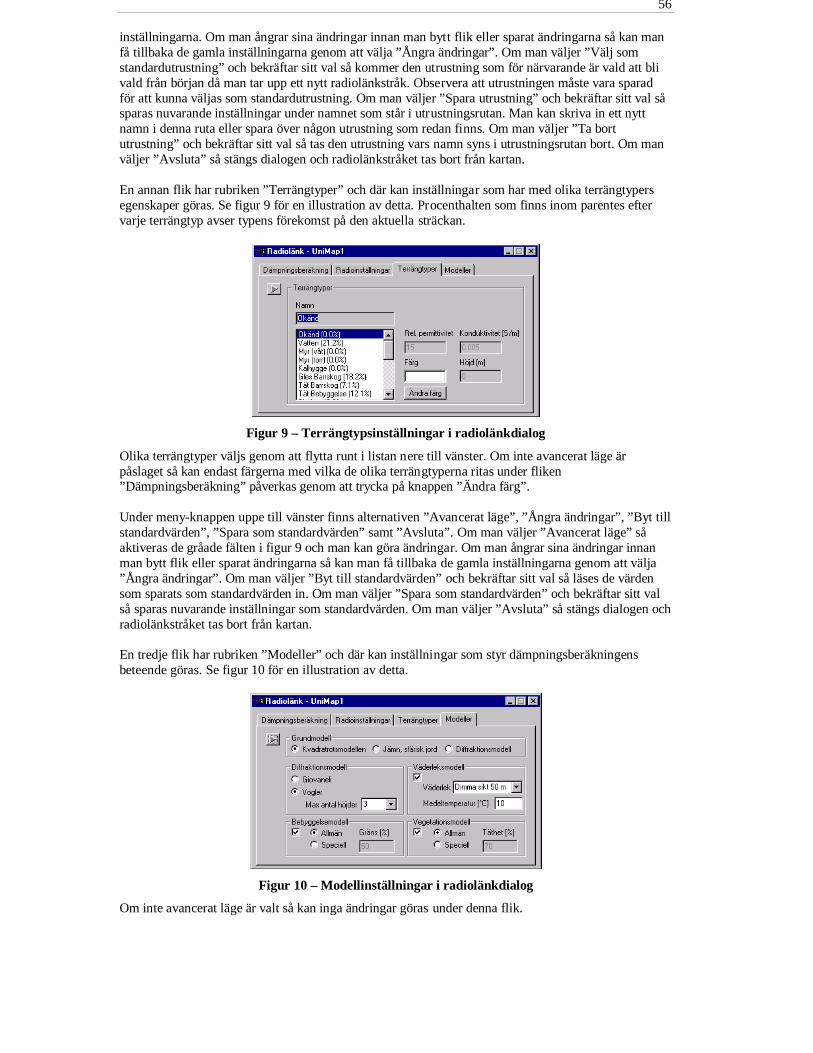
56

inställningarna. Om man ångrar sina ändringar innan man bytt flik eller sparat ändringarna så kan manfå tillbaka de gamla inställningarna genom att välja ”Ångra ändringar”. Om man väljer ”Välj somstandardutrustning” och bekräftar sitt val så kommer den utrustning som för närvarande är vald att blivald från början då man tar upp ett nytt radiolänkstråk. Observera att utrustningen måste vara sparadför att kunna väljas som standardutrustning. Om man väljer ”Spara utrustning” och bekräftar sitt val såsparas nuvarande inställningar under namnet som står i utrustningsrutan. Man kan skriva in ett nyttnamn i denna ruta eller spara över någon utrustning som redan finns. Om man väljer ”Ta bortutrustning” och bekräftar sitt val så tas den utrustning vars namn syns i utrustningsrutan bort. Om manväljer ”Avsluta” så stängs dialogen och radiolänkstråket tas bort från kartan.

En annan flik har rubriken ”Terrängtyper” och där kan inställningar som har med olika terrängtypersegenskaper göras. Se figur 9 för en illustration av detta. Procenthalten som finns inom parentes eftervarje terrängtyp avser typens förekomst på den aktuella sträckan.

Figur 9 – Terrängtypsinställningar i radiolänkdialog

Olika terrängtyper väljs genom att flytta runt i listan nere till vänster. Om inte avancerat läge ärpåslaget så kan endast färgerna med vilka de olika terrängtyperna ritas under fliken”Dämpningsberäkning” påverkas genom att trycka på knappen ”Ändra färg”.

Under meny-knappen uppe till vänster finns alternativen ”Avancerat läge”, ”Ångra ändringar”, ”Byt tillstandardvärden”, ”Spara som standardvärden” samt ”Avsluta”. Om man väljer ”Avancerat läge” såaktiveras de gråade fälten i figur 9 och man kan göra ändringar. Om man ångrar sina ändringar innanman bytt flik eller sparat ändringarna så kan man få tillbaka de gamla inställningarna genom att välja”Ångra ändringar”. Om man väljer ”Byt till standardvärden” och bekräftar sitt val så läses de värdensom sparats som standardvärden in. Om man väljer ”Spara som standardvärden” och bekräftar sitt valså sparas nuvarande inställningar som standardvärden. Om man väljer ”Avsluta” så stängs dialogen ochradiolänkstråket tas bort från kartan.

En tredje flik har rubriken ”Modeller” och där kan inställningar som styr dämpningsberäkningensbeteende göras. Se figur 10 för en illustration av detta.

Figur 10 – Modellinställningar i radiolänkdialog

Om inte avancerat läge är valt så kan inga ändringar göras under denna flik.

57

Under meny-knappen uppe till vänster finns alternativen ”Avancerat läge”, ”Ångra ändringar”, ”Byt tillstandardvärden”, ”Spara som standardvärden” samt ”Avsluta”. Om man väljer ”Avancerat läge” så kanman göra ändringar i inställningarna. Om man ångrar sina ändringar innan man bytt flik eller sparatändringarna så kan man få tillbaka de gamla inställningarna genom att välja ”Ångra ändringar”. Omman väljer ”Byt till standardvärden” och bekräftar sitt val så läses de värden som sparats somstandardvärden in. Om man väljer ”Spara som standardvärden” och bekräftar sitt val så sparasnuvarande inställningar som standardvärden. Om man väljer ”Avsluta” så stängs dialogen ochradiolänkstråket tas bort från kartan.

Grundmodellen (se figur 11) bestämmer om man vill vikta ihop tilläggsdämpningen som fås då manräknar med en jämn, sfärisk jordmodell med dämpningen man får då man tar hänsyn till omgivningenstopologi i en diffraktionsmodell eller ej. För att vikta ihop dessa två tilläggsdämpningar används den såkallade kvadratrotsmodellen. Om man väljer ”Jämn, sfärisk jord” så räknas endast denna dämpningmed och på motsvarande sätt om man väljer ”Diffraktionsmodell”.

Figur 11 – Grundmodell i radiolänkdialog

Som diffraktionsmodell (se figur 12) kan man välja antingen en mer exakt metod av Vogler som tar litelängre tid i anspråk eller en snabbare, men mindre exakt metod av Giovaneli. Man kan också välja hurmånga höjder som skall anses vara signifikanta och kunna väljas ut att ta med i beräkningen (1, 3, 7eller 15 stycken). Ju fler höjder man väljer att ta med, desto längre tid kan beräkningen ta i anspråk. Etttips är att använda Voglers metod med maximalt sju höjder, vilken ger ett hyfsat resultat efter intealltför lång tid. Det är inte säkert att maximalt antal höjder väljs ut utan beroende på en parameter somär proportionell mot våglängden så väljs inte höjder som ligger för nära varandra ut. Detta för att spridaut de valda höjderna och få en bättre approximation av terrängen. De signifikanta höjderna som valts utför beräkningen är de som man kan välja att visa under fliken ”Dämpningsberäkning”.

Figur 12 – Diffraktionsmodell i radiolänkdialog

Om man kryssar i rutan under ”Väderleksmodell” (se figur 13) så används ett par modeller frånNASA:s referenspublikation 1082(04) för att beräkna den tilläggsdämpning som fås vid olika typer avsvår väderlek. Man kan välja väderlek mellan olika mycket regn, dimma eller snö. Temperaturen gårendast att ändra och påverkar endast beräkningen då dimma är vald. Man kan välja två olika typer avsnö som väderlek men programmet innehåller ingen beräkningsmetod för denna dämpning såtilläggsdämpningen sätts endast till noll. Valen finns endast med som en förberedelse för en framtidaimplementering av lämplig modell.

Figur 13 – Väderleksmodell i radiolänkdialog

Om man kryssar i rutan under ”Bebyggelsemodell” (se figur 14) så kan man välja ”Allmän” varvidbebyggelsehöjder bara adderas till de totala höjder som används vid diffraktionsberäkningen. Om mandäremot väljer ”Speciell” så används en metod av Ibrahim-Parsons för att beräkna den extra dämpningsom tillkommer vid kommunikation i städer. Observera att det är upp till användaren att avgöra ommetoden är tillämpbar eller inte. Man har möjlighet att ställa in en gräns för hur många procent avvägen mellan sändare och mottagare som skall ha bebyggelse som terrängtyp för att dämpningen skallberäknas. Om en mindre procenthalt än den givna är täckt av bebyggelse så sätts tilläggsdämpningen

58

från bebyggelse till noll. Detta val finns för att modellen ger en grunddämpning även om sträckan ärhelt fri från bebyggelse vilket inte är ett önskvärt beteende.

Figur 14 – Bebyggelsemodell i radiolänkdialog

Om man kryssar i rutan under ”Vegetationsmodell” (se figur 15) så kan man välja ”Allmän” varvidskogshöjd bara adderas till de totala höjder som används vid diffraktionsberäkningen. Om man däremotväljer ”Speciell” så används en metod som beskrivs i ITU-R rapport 1145 för den dämpning somtillkommer vid kommunikation genom skog. Observera att det är upp till användaren att avgöra ommetoden är tillämpbar eller inte. Användaren måste även ställa in vilken täthet i procent som skogen påsträckan anses ha. Denna täthet har ett värde nära noll om all skog på sträckan är extremt gles och ettvärde nära hundra om all skog på sträckan är extremt tät.

Figur 15 – Vegetationsmodell i radiolänkdialog

B.3.2 Övriga inställningarUnder menyn ”Options” och undermenyn ”Terränganalys” kan man välja bland en uppsättning val förde andra verktygen. För terränginfoverktyget kan man endast välja ”Inställningar”, medan man förmålsikt, frisiktsgräns samt siktfält kan välja ”Inställningar” eller ”Ta bort alla”. Slutligen kan man välja”Terrängtyper för siktberäkningar”.

B.3.2.1 Inställningar för terränginfoverktygetDå man väljer inställningar för terränginformation så får man upp dialogrutan i figur 16.

Figur 16 – Inställningar för terränginfoverktyget

Om rutan är ikryssad så adderas terrängtypernas höjder till den höjd som anges då man använderterränginfoverktyget. Terrängtypernas höjder är de som ställs in under ”Terrängtyper –Siktberäkningar” (se avsnitt B.3.2.5).

B.3.2.2 Inställningar för målsiktverktygetDå man väljer inställningar för målsikt så får man upp dialogrutan i figur 17.

59

Figur 17 – Inställningar för målsiktverktyget

I dialogen kan man göra följande inställningar:

• Vad man vill att observatören skall ha för höjd (i meter).• Vad man vill att målet skall ha för höjd (i meter).• Om man vill att terrängtypernas höjder skall adderas till de höjder som används på sträckan.

Terrängtypernas höjder är de som ställs in under ”Terrängtyper – Siktberäkningar” (se avsnittB.3.2.5).

B.3.2.3 Inställningar för frisiktsgränsverktygetDå man väljer inställningar för frisiktsgräns så får man upp dialogrutan i figur 18.

Figur 18 – Inställningar för frisiktsgränsverktyget

I dialogen kan man göra följande inställningar:

• Vad man vill att observatören skall ha för höjd (i meter).• Om man vill att målsikt skall användas, d.v.s. att målets höjd över marken är mer än noll meter.• Om man valt målsikt, vad man vill att målet skall ha för höjd (i meter).• Om man vill använda den teoretiskt maximala sträckan som man kan se om jorden ses som en helt

jämn sfär. Denna horisont beräknas med en effektiv jordradie (4/3 av den verkliga) för att manskall kunna approximera strålgången med en rät linje.

• Om man inte valt att använda den teoretiska jordhorisonten så kan man fylla i en egendefinieradhorisont (i kilometer).

• Om man vill att terrängtypernas höjder skall adderas till de höjder som används på sträckan.Terrängtypernas höjder är de som ställs in under ”Terrängtyper – Siktberäkningar” (se avsnittB.3.2.5).

• Hur många vinklar man vill att verktyget skall använda då den söker runt mittpunkten. Observeraatt man med fler vinklar riskerar att stjärnformationer uppkommer.

• Hur bred frisiktsgränsen ritas (i pixels).

B.3.2.4 Inställningar för siktfältverktygetDå man väljer inställningar för siktfält så får man upp dialogrutan i figur 19.

60

Figur 19 – Inställningar för siktfältverktyget

I dialogen kan man göra följande inställningar:

• Vad man vill att observatören skall ha för höjd (i meter).• Om man vill att målsikt skall användas, d.v.s. att målets höjd över marken är mer än noll meter.• Om man valt målsikt, vad man vill att målet skall ha för höjd (i meter).• Om man vill använda den teoretiskt maximala sträckan som man kan se om jorden ses som en helt

jämn sfär. Denna horisont beräknas med en effektiv jordradie (4/3 av den verkliga) för att manskall kunna approximera strålgången med en rät linje.

• Om man inte valt att använda den teoretiska jordhorisonten så kan man fylla i en egendefinieradhorisont (i kilometer).

• Om man vill att terrängtypernas höjder skall adderas till de höjder som används på sträckan.Terrängtypernas höjder är de som ställs in under ”Terrängtyper – Siktberäkningar” (se avsnittB.3.2.5).

• Om man vill att beräkningar endast skall göras för den del av kartan som för tillfället syns ifönstret. Detta spar en hel del tid speciellt om man har zoomat in mycket i kartan.

• Hur långt mellanrum man vill ha mellan individuella punkter i siktfältet (i pixels). Observera atttalet egentligen anger hur många steg man minst vill ta mellan punkterna. Om detta tal väljs till ettså blir siktfältet maximalt tätt men tar lång tid att beräkna.

• Hur stora man vill att individuella punkter i siktfältet skall ritas (i pixels). Om detta tal väljs till ettoch punktmellanrummet väljs till ett så får man ett siktfält med maximal upplösning. Enrekommendation är att välja punktmellanrummet till fyra och punktstorleken till två vilket ger etthyfsat snyggt siktfält som inte tar alltför lång tid att beräkna.

B.3.2.5 Terrängtyper för siktberäkningarDå man väljer terrängtyper för siktberäkningar så får man upp dialogrutan i figur 20.

Figur 20 – Terrängtyper för siktberäkningar

I dialogen kan man ställa in hur höga man anser att de olika terrängtyperna är i medeltal. Dessa värdenanvänds vid beräkningarna i terränginfoverktyget, målsiktverktyget, frisiktsgränsverktyget samtsiktfältverktyget om man väljer att addera terrängbeklädnadens höjd. De terränghöjder som användsvid radiolänkberäkning ställs in i radiolänkdialogen (se avsnitt B.3.1).