Terence Tao Analysis I - Matej Bel University · Terence Tao Department of Mathematics University...

Texts and Readings in Mathematics 37

Analysis IThird Edition

Terence Tao

Texts and Readings in Mathematics

Volume 37

Advisory Editor

C.S. Seshadri, Chennai Mathematical Institute, Chennai

Managing Editor

Rajendra Bhatia, Indian Statistical Institute, New Delhi

Editor

Manindra Agrawal, Indian Institute of Technology Kanpur, KanpurV. Balaji, Chennai Mathematical Institute, ChennaiR.B. Bapat, Indian Statistical Institute, New DelhiV.S. Borkar, Indian Institute of Technology Bombay, MumbaiT.R. Ramadas, Chennai Mathematical Institute, ChennaiV. Srinivas, Tata Institute of Fundamental Research, Mumbai

The Texts and Readings in Mathematics series publishes high-quality textbooks,research-level monographs, lecture notes and contributed volumes. Undergraduateand graduate students of mathematics, research scholars, and teachers would findthis book series useful. The volumes are carefully written as teaching aids andhighlight characteristic features of the theory. The books in this series areco-published with Hindustan Book Agency, New Delhi, India.

More information about this series at http://www.springer.com/series/15141

http://www.springer.com/series/15141

Terence Tao

Analysis IThird Edition

123

Terence TaoDepartment of MathematicsUniversity of California, Los AngelesLos Angeles, CAUSA

This work is a co-publication with Hindustan Book Agency, New Delhi, licensed for sale in allcountries in electronic form only. Sold and distributed in print across the world by HindustanBookAgency, P-19Green Park Extension, NewDelhi 110016, India. ISBN: 978-93-80250-64-9© Hindustan Book Agency 2015.

ISSN 2366-8725 (electronic)Texts and Readings in MathematicsISBN 978-981-10-1789-6 (eBook)DOI 10.1007/978-981-10-1789-6

Library of Congress Control Number: 2016940817

© Springer Science+Business Media Singapore 2016 and Hindustan Book Agency 2015This work is subject to copyright. All rights are reserved by the Publishers, whether the whole or partof the material is concerned, specifically the rights of translation, reprinting, reuse of illustrations,recitation, broadcasting, reproduction on microfilms or in any other physical way, and transmissionor information storage and retrieval, electronic adaptation, computer software, or by similar or dissimilarmethodology now known or hereafter developed.The use of general descriptive names, registered names, trademarks, service marks, etc. in thispublication does not imply, even in the absence of a specific statement, that such names are exempt fromthe relevant protective laws and regulations and therefore free for general use.The publishers, the authors and the editors are safe to assume that the advice and information in thisbook are believed to be true and accurate at the date of publication. Neither the publishers nor theauthors or the editors give a warranty, express or implied, with respect to the material contained herein orfor any errors or omissions that may have been made.

This Springer imprint is published by Springer NatureThe registered company is Springer Science+Business Media Singapore Pte Ltd.

To my parents, for everything

Contents

1 Introduction 11.1 What is analysis? . . . . . . . . . . . . . . . . . . . . . . 11.2 Why do analysis? . . . . . . . . . . . . . . . . . . . . . . 2

2 Starting at the beginning: the natural numbers 132.1 The Peano axioms . . . . . . . . . . . . . . . . . . . . . . 152.2 Addition . . . . . . . . . . . . . . . . . . . . . . . . . . . 242.3 Multiplication . . . . . . . . . . . . . . . . . . . . . . . . 29

3 Set theory 333.1 Fundamentals . . . . . . . . . . . . . . . . . . . . . . . . 333.2 Russell’s paradox (Optional) . . . . . . . . . . . . . . . . 463.3 Functions . . . . . . . . . . . . . . . . . . . . . . . . . . . 493.4 Images and inverse images . . . . . . . . . . . . . . . . . 563.5 Cartesian products . . . . . . . . . . . . . . . . . . . . . 623.6 Cardinality of sets . . . . . . . . . . . . . . . . . . . . . . 67

4 Integers and rationals 744.1 The integers . . . . . . . . . . . . . . . . . . . . . . . . . 744.2 The rationals . . . . . . . . . . . . . . . . . . . . . . . . . 814.3 Absolute value and exponentiation . . . . . . . . . . . . . 864.4 Gaps in the rational numbers . . . . . . . . . . . . . . . . 90

5 The real numbers 945.1 Cauchy sequences . . . . . . . . . . . . . . . . . . . . . . 965.2 Equivalent Cauchy sequences . . . . . . . . . . . . . . . . 1005.3 The construction of the real numbers . . . . . . . . . . . 1025.4 Ordering the reals . . . . . . . . . . . . . . . . . . . . . . 111

Preface to the first edition

xi

xiii

xixAbout the Author

vii

Preface to the second and third editions

Contents

5.5 The least upper bound property . . . . . . . . . . . . . . 116

5.6 Real exponentiation, part I . . . . . . . . . . . . . . . . . 121

6 Limits of sequences 126

6.1 Convergence and limit laws . . . . . . . . . . . . . . . . . 126

6.2 The Extended real number system . . . . . . . . . . . . . 133

6.3 Suprema and Infima of sequences . . . . . . . . . . . . . 137

6.4 Limsup, Liminf, and limit points . . . . . . . . . . . . . . 139

6.5 Some standard limits . . . . . . . . . . . . . . . . . . . . 148

6.6 Subsequences . . . . . . . . . . . . . . . . . . . . . . . . . 149

6.7 Real exponentiation, part II . . . . . . . . . . . . . . . . 152

7 Series 155

7.1 Finite series . . . . . . . . . . . . . . . . . . . . . . . . . 155

7.2 Infinite series . . . . . . . . . . . . . . . . . . . . . . . . . 164

7.3 Sums of non-negative numbers . . . . . . . . . . . . . . . 170

7.4 Rearrangement of series . . . . . . . . . . . . . . . . . . . 174

7.5 The root and ratio tests . . . . . . . . . . . . . . . . . . . 178

8 Infinite sets 181

8.1 Countability . . . . . . . . . . . . . . . . . . . . . . . . . 181

8.2 Summation on infinite sets . . . . . . . . . . . . . . . . . 188

8.3 Uncountable sets . . . . . . . . . . . . . . . . . . . . . . . 195

8.4 The axiom of choice . . . . . . . . . . . . . . . . . . . . . 198

8.5 Ordered sets . . . . . . . . . . . . . . . . . . . . . . . . . 202

9 Continuous functions on R 211

9.1 Subsets of the real line . . . . . . . . . . . . . . . . . . . 211

9.2 The algebra of real-valued functions . . . . . . . . . . . . 217

9.3 Limiting values of functions . . . . . . . . . . . . . . . . 220

9.4 Continuous functions . . . . . . . . . . . . . . . . . . . . 227

9.5 Left and right limits . . . . . . . . . . . . . . . . . . . . . 231

9.6 The maximum principle . . . . . . . . . . . . . . . . . . . 234

9.7 The intermediate value theorem . . . . . . . . . . . . . . 238

9.8 Monotonic functions . . . . . . . . . . . . . . . . . . . . . 241

9.9 Uniform continuity . . . . . . . . . . . . . . . . . . . . . 243

9.10 Limits at infinity . . . . . . . . . . . . . . . . . . . . . . . 249

10 Differentiation of functions 251

10.1 Basic definitions . . . . . . . . . . . . . . . . . . . . . . . 251

viii

Contents

10.2 Local maxima, local minima, and derivatives . . . . . . . 25710.3 Monotone functions and derivatives . . . . . . . . . . . . 26010.4 Inverse functions and derivatives . . . . . . . . . . . . . . 26110.5 L’Hopital’s rule . . . . . . . . . . . . . . . . . . . . . . . 264

11 The Riemann integral 26711.1 Partitions . . . . . . . . . . . . . . . . . . . . . . . . . . . 26811.2 Piecewise constant functions . . . . . . . . . . . . . . . . 27211.3 Upper and lower Riemann integrals . . . . . . . . . . . . 27611.4 Basic properties of the Riemann integral . . . . . . . . . 28011.5 Riemann integrability of continuous functions . . . . . . 28511.6 Riemann integrability of monotone functions . . . . . . . 28911.7 A non-Riemann integrable function . . . . . . . . . . . . 29111.8 The Riemann-Stieltjes integral . . . . . . . . . . . . . . . 29211.9 The two fundamental theorems of calculus . . . . . . . . 29511.10 Consequences of the fundamental theorems . . . . . . . . 300

A Appendix: the basics of mathematical logic 305A.1 Mathematical statements . . . . . . . . . . . . . . . . . . 306A.2 Implication . . . . . . . . . . . . . . . . . . . . . . . . . . 312A.3 The structure of proofs . . . . . . . . . . . . . . . . . . . 317A.4 Variables and quantifiers . . . . . . . . . . . . . . . . . . 320A.5 Nested quantifiers . . . . . . . . . . . . . . . . . . . . . . 324A.6 Some examples of proofs and quantifiers . . . . . . . . . 327A.7 Equality . . . . . . . . . . . . . . . . . . . . . . . . . . . 329

B Appendix: the decimal system 331B.1 The decimal representation of natural numbers . . . . . . 332B.2 The decimal representation of real numbers . . . . . . . . 335

Index 339

349Texts and Readings in Mathematics

ix

Preface to the second and third editions

Since the publication of the first edition, many students and lectur-ers have communicated a number of minor typos and other correctionsto me. There was also some demand for a hardcover edition of thetexts. Because of this, the publishers and I have decided to incorporatethe corrections and issue a hardcover second edition of the textbooks.The layout, page numbering, and indexing of the texts have also beenchanged; in particular the two volumes are now numbered and indexedseparately. However, the chapter and exercise numbering, as well as themathematical content, remains the same as the first edition, and so thetwo editions can be used more or less interchangeably for homework andstudy purposes.

The third edition contains a number of corrections that were reportedfor the second edition, together with a few new exercises, but is otherwiseessentially the same text.

xi


This text originated from the lecture notes I gave teaching the honoursundergraduate-level real analysis sequence at the University of Califor-nia, Los Angeles, in 2003. Among the undergraduates here, real anal-ysis was viewed as being one of the most difficult courses to learn, notonly because of the abstract concepts being introduced for the first time(e.g., topology, limits, measurability, etc.), but also because of the levelof rigour and proof demanded of the course. Because of this percep-tion of difficulty, one was often faced with the difficult choice of eitherreducing the level of rigour in the course in order to make it easier, orto maintain strict standards and face the prospect of many undergradu-ates, even many of the bright and enthusiastic ones, struggling with thecourse material.

Faced with this dilemma, I tried a somewhat unusual approach tothe subject. Typically, an introductory sequence in real analysis assumesthat the students are already familiar with the real numbers, with math-ematical induction, with elementary calculus, and with the basics of settheory, and then quickly launches into the heart of the subject, for in-stance the concept of a limit. Normally, students entering this sequencedo indeed have a fair bit of exposure to these prerequisite topics, thoughin most cases the material is not covered in a thorough manner. For in-stance, very few students were able to actually define a real number, oreven an integer, properly, even though they could visualize these num-bers intuitively and manipulate them algebraically. This seemed to meto be a missed opportunity. Real analysis is one of the first subjects(together with linear algebra and abstract algebra) that a student en-counters, in which one truly has to grapple with the subtleties of a trulyrigorous mathematical proof. As such, the course offered an excellentchance to go back to the foundations of mathematics, and in particular

xiii


the opportunity to do a proper and thorough construction of the realnumbers.

Thus the course was structured as follows. In the first week, I de-scribed some well-known “paradoxes” in analysis, in which standard lawsof the subject (e.g., interchange of limits and sums, or sums and inte-grals) were applied in a non-rigorous way to give nonsensical results suchas 0 = 1. This motivated the need to go back to the very beginning of thesubject, even to the very definition of the natural numbers, and checkall the foundations from scratch. For instance, one of the first homeworkassignments was to check (using only the Peano axioms) that additionwas associative for natural numbers (i.e., that (a+ b) + c = a+ (b+ c)for all natural numbers a, b, c: see Exercise 2.2.1). Thus even in thefirst week, the students had to write rigorous proofs using mathematicalinduction. After we had derived all the basic properties of the naturalnumbers, we then moved on to the integers (initially defined as formaldifferences of natural numbers); once the students had verified all thebasic properties of the integers, we moved on to the rationals (initiallydefined as formal quotients of integers); and then from there we movedon (via formal limits of Cauchy sequences) to the reals. Around thesame time, we covered the basics of set theory, for instance demonstrat-ing the uncountability of the reals. Only then (after about ten lectures)did we begin what one normally considers the heart of undergraduatereal analysis - limits, continuity, differentiability, and so forth.

The response to this format was quite interesting. In the first fewweeks, the students found the material very easy on a conceptual level,as we were dealing only with the basic properties of the standard num-ber systems. But on an intellectual level it was very challenging, as onewas analyzing these number systems from a foundational viewpoint, inorder to rigorously derive the more advanced facts about these numbersystems from the more primitive ones. One student told me how difficultit was to explain to his friends in the non-honours real analysis sequence(a) why he was still learning how to show why all rational numbersare either positive, negative, or zero (Exercise 4.2.4), while the non-honours sequence was already distinguishing absolutely convergent andconditionally convergent series, and (b) why, despite this, he thoughthis homework was significantly harder than that of his friends. Anotherstudent commented to me, quite wryly, that while she could obviouslysee why one could always divide a natural number n into a positiveinteger q to give a quotient a and a remainder r less than q (Exercise2.3.5), she still had, to her frustration, much difficulty in writing down

xiv


a proof of this fact. (I told her that later in the course she would haveto prove statements for which it would not be as obvious to see thatthe statements were true; she did not seem to be particularly consoledby this.) Nevertheless, these students greatly enjoyed the homework, aswhen they did perservere and obtain a rigorous proof of an intuitive fact,it solidified the link in their minds between the abstract manipulationsof formal mathematics and their informal intuition of mathematics (andof the real world), often in a very satisfying way. By the time they wereassigned the task of giving the infamous “epsilon and delta” proofs inreal analysis, they had already had so much experience with formalizingintuition, and in discerning the subtleties of mathematical logic (suchas the distinction between the “for all” quantifier and the “there exists”quantifier), that the transition to these proofs was fairly smooth, and wewere able to cover material both thoroughly and rapidly. By the tenthweek, we had caught up with the non-honours class, and the studentswere verifying the change of variables formula for Riemann-Stieltjes in-tegrals, and showing that piecewise continuous functions were Riemannintegrable. By the conclusion of the sequence in the twentieth week, wehad covered (both in lecture and in homework) the convergence theory ofTaylor and Fourier series, the inverse and implicit function theorem forcontinuously differentiable functions of several variables, and establishedthe dominated convergence theorem for the Lebesgue integral.

In order to cover this much material, many of the key foundationalresults were left to the student to prove as homework; indeed, this wasan essential aspect of the course, as it ensured the students truly ap-preciated the concepts as they were being introduced. This format hasbeen retained in this text; the majority of the exercises consist of provinglemmas, propositions and theorems in the main text. Indeed, I wouldstrongly recommend that one do as many of these exercises as possible- and this includes those exercises proving “obvious” statements - if onewishes to use this text to learn real analysis; this is not a subject whosesubtleties are easily appreciated just from passive reading. Most of thechapter sections have a number of exercises, which are listed at the endof the section.

To the expert mathematician, the pace of this book may seem some-what slow, especially in early chapters, as there is a heavy emphasison rigour (except for those discussions explicitly marked “Informal”),and justifying many steps that would ordinarily be quickly passed overas being self-evident. The first few chapters develop (in painful detail)many of the “obvious” properties of the standard number systems, for

xv


instance that the sum of two positive real numbers is again positive (Ex-ercise 5.4.1), or that given any two distinct real numbers, one can findrational number between them (Exercise 5.4.5). In these foundationalchapters, there is also an emphasis on non-circularity - not using later,more advanced results to prove earlier, more primitive ones. In partic-ular, the usual laws of algebra are not used until they are derived (andthey have to be derived separately for the natural numbers, integers,rationals, and reals). The reason for this is that it allows the studentsto learn the art of abstract reasoning, deducing true facts from a lim-ited set of assumptions, in the friendly and intuitive setting of numbersystems; the payoff for this practice comes later, when one has to utilizethe same type of reasoning techniques to grapple with more advancedconcepts (e.g., the Lebesgue integral).

The text here evolved from my lecture notes on the subject, andthus is very much oriented towards a pedagogical perspective; muchof the key material is contained inside exercises, and in many cases Ihave chosen to give a lengthy and tedious, but instructive, proof in-stead of a slick abstract proof. In more advanced textbooks, the studentwill see shorter and more conceptually coherent treatments of this ma-terial, and with more emphasis on intuition than on rigour; however,I feel it is important to know how to do analysis rigorously and “byhand” first, in order to truly appreciate the more modern, intuitive andabstract approach to analysis that one uses at the graduate level andbeyond.

The exposition in this book heavily emphasizes rigour and formal-ism; however this does not necessarily mean that lectures based onthis book have to proceed the same way. Indeed, in my own teach-ing I have used the lecture time to present the intuition behind theconcepts (drawing many informal pictures and giving examples), thusproviding a complementary viewpoint to the formal presentation in thetext. The exercises assigned as homework provide an essential bridgebetween the two, requiring the student to combine both intuition andformal understanding together in order to locate correct proofs for aproblem. This I found to be the most difficult task for the students,as it requires the subject to be genuinely learnt, rather than merelymemorized or vaguely absorbed. Nevertheless, the feedback I receivedfrom the students was that the homework, while very demanding forthis reason, was also very rewarding, as it allowed them to connect therather abstract manipulations of formal mathematics with their innateintuition on such basic concepts as numbers, sets, and functions. Of

xvi


course, the aid of a good teaching assistant is invaluable in achieving thisconnection.

With regard to examinations for a course based on this text, I wouldrecommend either an open-book, open-notes examination with problemssimilar to the exercises given in the text (but perhaps shorter, with nounusual trickery involved), or else a take-home examination that involvesproblems comparable to the more intricate exercises in the text. Thesubject matter is too vast to force the students to memorize the defini-tions and theorems, so I would not recommend a closed-book examina-tion, or an examination based on regurgitating extracts from the book.(Indeed, in my own examinations I gave a supplemental sheet listing thekey definitions and theorems which were relevant to the examinationproblems.) Making the examinations similar to the homework assignedin the course will also help motivate the students to work through andunderstand their homework problems as thoroughly as possible (as op-posed to, say, using flash cards or other such devices to memorize mate-rial), which is good preparation not only for examinations but for doingmathematics in general.

Some of the material in this textbook is somewhat peripheral tothe main theme and may be omitted for reasons of time constraints.For instance, as set theory is not as fundamental to analysis as arethe number systems, the chapters on set theory (Chapters 3, 8) can becovered more quickly and with substantially less rigour, or be given asreading assignments. The appendices on logic and the decimal systemare intended as optional or supplemental reading and would probablynot be covered in the main course lectures; the appendix on logic isparticularly suitable for reading concurrently with the first few chapters.Also, Chapter 11.27 (on Fourier series) is not needed elsewhere in thetext and can be omitted.

For reasons of length, this textbook has been split into two volumes.The first volume is slightly longer, but can be covered in about thirtylectures if the peripheral material is omitted or abridged. The secondvolume refers at times to the first, but can also be taught to studentswho have had a first course in analysis from other sources. It also takesabout thirty lectures to cover.

I am deeply indebted to my students, who over the progression ofthe real analysis course corrected several errors in the lectures notesfrom which this text is derived, and gave other valuable feedback. I amalso very grateful to the many anonymous referees who made severalcorrections and suggested many important improvements to the text.

xvii


I also thank Biswaranjan Behera, Tai-Danae Bradley, Brian, EduardoBuscicchio, Carlos, EO, Florian, Gokhan Guclu, Evangelos Georgiadis,Ulrich Groh, Bart Kleijngeld, Erik Koelink, Wang Kuyyang, MatthisLehmkuhler, Percy Li, Ming Li, Jason M., Manoranjan Majji, GeoffMess, Pieter Naaijkens, Vineet Nair, Cristina Pereyra, David Radnell,Tim Reijnders, Pieter Roffelsen, Luke Rogers, Marc Schoolderman, KentVan Vels, Daan Wanrooy, Yandong Xiao, Sam Xu, Luqing Ye, and thestudents of Math 401/501 and Math 402/502 at the University of NewMexico for corrections to the first and second editions.

Terence Tao

xviii

xix

About the Author

Terence Tao, FAA FRS, is an Australian mathematician. His areas of interests arein harmonic analysis, partial differential equations, algebraic combinatorics, arith-metic combinatorics, geometric combinatorics, compressed sensing and analyticnumber theory. As of 2015, he holds the James and Carol Collins chair in math-ematics at the University of California, Los Angeles. Professor Tao is a co-recipientof the 2006 Fields Medal and the 2014 Breakthrough Prize in Mathematics. Hemaintains a personal mathematics blog, which has been described by TimothyGowers as “the undisputed king of all mathematics blogs”.

Chapter 1

Introduction

1.1 What is analysis?

This text is an honours-level undergraduate introduction to real analy-sis: the analysis of the real numbers, sequences and series of real num-bers, and real-valued functions. This is related to, but is distinct from,complex analysis, which concerns the analysis of the complex numbersand complex functions, harmonic analysis, which concerns the analy-sis of harmonics (waves) such as sine waves, and how they synthesizeother functions via the Fourier transform, functional analysis, which fo-cuses much more heavily on functions (and how they form things likevector spaces), and so forth. Analysis is the rigorous study of suchobjects, with a focus on trying to pin down precisely and accuratelythe qualitative and quantitative behavior of these objects. Real analy-sis is the theoretical foundation which underlies calculus, which is thecollection of computational algorithms which one uses to manipulatefunctions.

In this text we will be studying many objects which will be familiarto you from freshman calculus: numbers, sequences, series, limits, func-tions, definite integrals, derivatives, and so forth. You already have agreat deal of experience of computing with these objects; however herewe will be focused more on the underlying theory for these objects. Wewill be concerned with questions such as the following:

1. What is a real number? Is there a largest real number? After 0,what is the “next” real number (i.e., what is the smallest positivereal number)? Can you cut a real number into pieces infinitelymany times? Why does a number such as 2 have a square root,while a number such as -2 does not? If there are infinitely many

1� Springer Science+Business Media Singapore 2016 and Hindustan Book Agency 2015T. Tao, Analysis I, Texts and Readings in Mathematics 37,DOI 10.1007/978-981-10-1789-6_1

2 1. Introduction

reals and infinitely many rationals, how come there are “more”real numbers than rational numbers?

2. How do you take the limit of a sequence of real numbers? Whichsequences have limits and which ones don’t? If you can stop asequence from escaping to infinity, does this mean that it musteventually settle down and converge? Can you add infinitely manyreal numbers together and still get a finite real number? Can youadd infinitely many rational numbers together and end up with anon-rational number? If you rearrange the elements of an infinitesum, is the sum still the same?

3. What is a function? What does it mean for a function to becontinuous? differentiable? integrable? bounded? Can you addinfinitely many functions together? What about taking limits ofsequences of functions? Can you differentiate an infinite series offunctions? What about integrating? If a function f(x) takes thevalue 3 when x = 0 and 5 when x = 1 (i.e., f(0) = 3 and f(1) = 5),does it have to take every intermediate value between 3 and 5 whenx goes between 0 and 1? Why?

You may already know how to answer some of these questions fromyour calculus classes, but most likely these sorts of issues were only ofsecondary importance to those courses; the emphasis was on getting youto perform computations, such as computing the integral of x sin(x2)from x = 0 to x = 1. But now that you are comfortable with theseobjects and already know how to do all the computations, we will goback to the theory and try to really understand what is going on.

1.2 Why do analysis?

It is a fair question to ask, “why bother?”, when it comes to analysis.There is a certain philosophical satisfaction in knowing why things work,but a pragmatic person may argue that one only needs to know howthings work to do real-life problems. The calculus training you receive inintroductory classes is certainly adequate for you to begin solving manyproblems in physics, chemistry, biology, economics, computer science,finance, engineering, or whatever else you end up doing - and you cancertainly use things like the chain rule, L’Hopital’s rule, or integrationby parts without knowing why these rules work, or whether there areany exceptions to these rules. However, one can get into trouble if

1.2. Why do analysis? 3

one applies rules without knowing where they came from and what thelimits of their applicability are. Let me give some examples in whichseveral of these familiar rules, if applied blindly without knowledge ofthe underlying analysis, can lead to disaster.

Example 1.2.1 (Division by zero). This is a very familiar one to you:the cancellation law ac = bc =⇒ a = b does not work when c = 0. Forinstance, the identity 1× 0 = 2× 0 is true, but if one blindly cancels the0 then one obtains 1 = 2, which is false. In this case it was obvious thatone was dividing by zero; but in other cases it can be more hidden.

Example 1.2.2 (Divergent series). You have probably seen geometricseries such as the infinite sum

S = 1 +1

2+

1

4+

1

8+

1

16+ . . . .

You have probably seen the following trick to sum this series: if we callthe above sum S, then if we multiply both sides by 2, we obtain

2S = 2 + 1 +1

2+

1

4+

1

8+ . . . = 2 + S

and hence S = 2, so the series sums to 2. However, if you apply thesame trick to the series

S = 1 + 2 + 4 + 8 + 16 + . . .

one gets nonsensical results:

2S = 2 + 4 + 8 + 16 + . . . = S − 1 =⇒ S = −1.

So the same reasoning that shows that 1 + 12 + 1

4 + . . . = 2 also givesthat 1 + 2+ 4+ 8+ . . . = −1. Why is it that we trust the first equationbut not the second? A similar example arises with the series

S = 1− 1 + 1− 1 + 1− 1 + . . . ;

we can write

S = 1− (1− 1 + 1− 1 + . . .) = 1− S

and hence that S = 1/2; or instead we can write

S = (1− 1) + (1− 1) + (1− 1) + . . . = 0 + 0 + . . .

4 1. Introduction

and hence that S = 0; or instead we can write

S = 1 + (−1 + 1) + (−1 + 1) + . . . = 1 + 0 + 0 + . . .

and hence that S = 1. Which one is correct? (See Exercise 7.2.1 for ananswer.)

Example 1.2.3 (Divergent sequences). Here is a slight variation of theprevious example. Let x be a real number, and let L be the limit

L = limn→∞xn.

Changing variables n = m+ 1, we have

L = limm+1→∞

xm+1 = limm+1→∞

x× xm = x limm+1→∞

xm.

But if m+ 1 → ∞, then m → ∞, thus

limm+1→∞

xm = limm→∞xm = lim

n→∞xn = L,

and thus

xL = L.

At this point we could cancel the L’s and conclude that x = 1 for anarbitrary real number x, which is absurd. But since we are alreadyaware of the division by zero problem, we could be a little smarter andconclude instead that either x = 1, or L = 0. In particular we seem tohave shown that

limn→∞xn = 0 for all x �= 1.

But this conclusion is absurd if we apply it to certain values of x, forinstance by specializing to the case x = 2 we could conclude that thesequence 1, 2, 4, 8, . . . converges to zero, and by specializing to the casex = −1 we conclude that the sequence 1,−1, 1,−1, . . . also converges tozero. These conclusions appear to be absurd; what is the problem withthe above argument? (See Exercise 6.3.4 for an answer.)

Example 1.2.4 (Limiting values of functions). Start with the expres-sion limx→∞ sin(x), make the change of variable x = y + π and recallthat sin(y + π) = − sin(y) to obtain

limx→∞ sin(x) = lim

y+π→∞ sin(y + π) = limy→∞(− sin(y)) = − lim

y→∞ sin(y).


Since limx→∞ sin(x) = limy→∞ sin(y) we thus have

limx→∞ sin(x) = − lim

x→∞ sin(x)

and hence

limx→∞ sin(x) = 0.

If we then make the change of variables x = π/2 + z and recall thatsin(π/2 + z) = cos(z) we conclude that

limx→∞ cos(x) = 0.

Squaring both of these limits and adding we see that

limx→∞(sin2(x) + cos2(x)) = 02 + 02 = 0.

On the other hand, we have sin2(x) + cos2(x) = 1 for all x. Thus wehave shown that 1 = 0! What is the difficulty here?

Example 1.2.5 (Interchanging sums). Consider the following fact ofarithmetic. Consider any matrix of numbers, e.g.

⎛⎝ 1 2 3

4 5 67 8 9

⎞⎠

and compute the sums of all the rows and the sums of all the columns,and then total all the row sums and total all the column sums. In bothcases you will get the same number - the total sum of all the entries inthe matrix: ⎛

⎝ 1 2 34 5 67 8 9

⎞⎠ 6

1524

12 15 18 45

To put it another way, if you want to add all the entries in an m × nmatrix together, it doesn’t matter whether you sum the rows first orsum the columns first, you end up with the same answer. (Before theinvention of computers, accountants and book-keepers would use thisfact to guard against making errors when balancing their books.) In

6 1. Introduction

series notation, this fact would be expressed as

m∑i=1

n∑j=1

aij =

n∑j=1

m∑i=1

aij ,

if aij denoted the entry in the ith row and jth column of the matrix.Now one might think that this rule should extend easily to infinite

series:∞∑i=1

∞∑j=1

aij =

∞∑j=1

∞∑i=1

aij .

Indeed, if you use infinite series a lot in your work, you will find yourselfhaving to switch summations like this fairly often. Another way of sayingthis fact is that in an infinite matrix, the sum of the row-totals shouldequal the sum of the column-totals. However, despite the reasonablenessof this statement, it is actually false! Here is a counterexample:

⎛⎜⎜⎜⎜⎜⎜⎜⎝

1 0 0 0 . . .−1 1 0 0 . . .0 −1 1 0 . . .0 0 −1 1 . . .0 0 0 −1 . . ....

......

.... . .

⎞⎟⎟⎟⎟⎟⎟⎟⎠

.

If you sum up all the rows, and then add up all the row totals, you get1; but if you sum up all the columns, and add up all the column totals,you get 0! So, does this mean that summations for infinite series shouldnot be swapped, and that any argument using such a swapping shouldbe distrusted? (See Theorem 8.2.2 for an answer.)

Example 1.2.6 (Interchanging integrals). The interchanging of inte-grals is a trick which occurs in mathematics just as commonly as theinterchanging of sums. Suppose one wants to compute the volume un-der a surface z = f(x, y) (let us ignore the limits of integration for themoment). One can do it by slicing parallel to the x-axis: for each fixedvalue of y, we can compute an area

∫f(x, y) dx, and then we integrate

the area in the y variable to obtain the volume

V =

∫ ∫f(x, y)dxdy.


Or we could slice parallel to the y-axis for each fixed x and compute anarea

∫f(x, y) dy, and then integrate in the x-axis to obtain

V =

∫ ∫f(x, y)dydx.

This seems to suggest that one should always be able to swap integralsigns: ∫ ∫

f(x, y) dxdy =

∫ ∫f(x, y) dydx.

And indeed, people swap integral signs all the time, because sometimesone variable is easier to integrate in first than the other. However, just asinfinite sums sometimes cannot be swapped, integrals are also sometimesdangerous to swap. An example is with the integrand e−xy − xye−xy.Suppose we believe that we can swap the integrals:

∫ ∞

0

∫ 1

0(e−xy − xye−xy) dy dx =

∫ 1

0

∫ ∞

0(e−xy − xye−xy) dx dy. (1.1)

Since ∫ 1

0(e−xy − xye−xy) dy = ye−xy|y=1

y=0 = e−x,

the left-hand side of (1.1) is∫∞0 e−x dx = −e−x|∞0 = 1. But since

∫ ∞

0(e−xy − xye−xy) dx = xe−xy|x=∞

x=0 = 0,

the right-hand side of (1.1) is∫ 10 0 dx = 0. Clearly 1 �= 0, so there is an

error somewhere; but you won’t find one anywhere except in the stepwhere we interchanged the integrals. So how do we know when to trustthe interchange of integrals? (See Theorem 11.50.1 for a partial answer.)

Example 1.2.7 (Interchanging limits). Suppose we start with the plau-sible looking statement

limx→0

limy→0

x2

x2 + y2= lim

y→0limx→0

x2

x2 + y2. (1.2)

But we have

limy→0

x2

x2 + y2=

x2

x2 + 02= 1,

8 1. Introduction

so the left-hand side of (1.2) is 1; on the other hand, we have

limx→0

x2

x2 + y2=

02

02 + y2= 0,

so the right-hand side of (1.2) is 0. Since 1 is clearly not equal to zero,this suggests that interchange of limits is untrustworthy. But are thereany other circumstances in which the interchange of limits is legitimate?(See Exercise 11.9.9 for a partial answer.)

Example 1.2.8 (Interchanging limits, again). Consider the plausiblelooking statement

limx→1−

limn→∞xn = lim

n→∞ limx→1−

xn

where the notation x → 1− means that x is approaching 1 from theleft. When x is to the left of 1, then limn→∞ xn = 0, and hence theleft-hand side is zero. But we also have limx→1− xn = 1 for all n, and sothe right-hand side limit is 1. Does this demonstrate that this type oflimit interchange is always untrustworthy? (See Proposition 11.15.3 foran answer.)

Example 1.2.9 (Interchanging limits and integrals). For any real num-ber y, we have∫ ∞

−∞

1

1 + (x− y)2dx = arctan(x− y)|∞x=−∞ =

π

2−(−π

2

)= π.

Taking limits as y → ∞, we should obtain∫ ∞

−∞limy→∞

1

1 + (x− y)2dx = lim

y→∞

∫ ∞

−∞1

1 + (x− y)2dx = π.

But for every x, we have limy→∞ 11+(x−y)2

= 0. So we seem to have

concluded that 0 = π. What was the problem with the above argument?Should one abandon the (very useful) technique of interchanging limitsand integrals? (See Theorem 11.18.1 for a partial answer.)

Example 1.2.10 (Interchanging limits and derivatives). Observe thatif ε > 0, then

d

dx

(x3

ε2 + x2

)=

3x2(ε2 + x2)− 2x4

(ε2 + x2)2


and in particular that

d

dx

(x3

ε2 + x2

)|x=0 = 0.

Taking limits as ε → 0, one might then expect that

d

dx

(x3

0 + x2

)|x=0 = 0.

But the right-hand side is ddxx = 1. Does this mean that it is always

illegitimate to interchange limits and derivatives? (See Theorem 11.19.1for an answer.)

Example 1.2.11 (Interchanging derivatives). Let1 f(x, y) be the func-

tion f(x, y) := xy3

x2+y2. A common maneuvre in analysis is to interchange

two partial derivatives, thus one expects

∂2f

∂x∂y(0, 0) =

∂2f

∂y∂x(0, 0).

But from the quotient rule we have

∂f

∂y(x, y) =

3xy2

x2 + y2− 2xy4

(x2 + y2)2

and in particular∂f

∂y(x, 0) =

0

x2− 0

x4= 0.

Thus∂2f

∂x∂y(0, 0) = 0.

On the other hand, from the quotient rule again we have

∂f

∂x(x, y) =

y3

x2 + y2− 2x2y3

(x2 + y2)2

and hence∂f

∂x(0, y) =

y3

y2− 0

y4= y.

1One might object that this function is not defined at (x, y) = (0, 0), but if we setf(0, 0) := (0, 0) then this function becomes continuous and differentiable for all (x, y),and in fact both partial derivatives ∂f

∂x, ∂f

∂yare also continuous and differentiable for

all (x, y)!

10 1. Introduction

Thus∂2f

∂y∂x(0, 0) = 1.

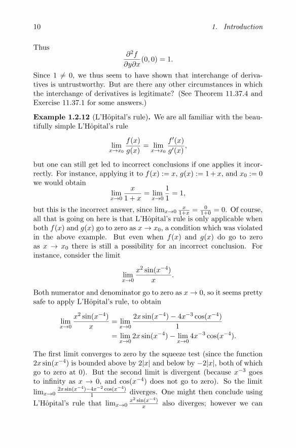
Since 1 �= 0, we thus seem to have shown that interchange of deriva-tives is untrustworthy. But are there any other circumstances in whichthe interchange of derivatives is legitimate? (See Theorem 11.37.4 andExercise 11.37.1 for some answers.)

Example 1.2.12 (L’Hopital’s rule). We are all familiar with the beau-tifully simple L’Hopital’s rule

limx→x0

f(x)

g(x)= lim

x→x0

f ′(x)g′(x)

,

but one can still get led to incorrect conclusions if one applies it incor-rectly. For instance, applying it to f(x) := x, g(x) := 1+x, and x0 := 0we would obtain

limx→0

x

1 + x= lim

x→0

1

1= 1,

but this is the incorrect answer, since limx→0x

1+x = 01+0 = 0. Of course,

all that is going on here is that L’Hopital’s rule is only applicable whenboth f(x) and g(x) go to zero as x → x0, a condition which was violatedin the above example. But even when f(x) and g(x) do go to zeroas x → x0 there is still a possibility for an incorrect conclusion. Forinstance, consider the limit

limx→0

x2 sin(x−4)

x.

Both numerator and denominator go to zero as x → 0, so it seems prettysafe to apply L’Hopital’s rule, to obtain

limx→0

x2 sin(x−4)

x= lim

x→0

2x sin(x−4)− 4x−3 cos(x−4)

1

= limx→0

2x sin(x−4)− limx→0

4x−3 cos(x−4).

The first limit converges to zero by the squeeze test (since the function2x sin(x−4) is bounded above by 2|x| and below by −2|x|, both of whichgo to zero at 0). But the second limit is divergent (because x−3 goesto infinity as x → 0, and cos(x−4) does not go to zero). So the limit

limx→02x sin(x−4)−4x−2 cos(x−4)

1 diverges. One might then conclude using

L’Hopital’s rule that limx→0x2 sin(x−4)

x also diverges; however we can


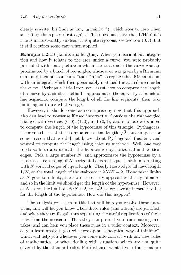
clearly rewrite this limit as limx→0 x sin(x−4), which goes to zero when

x → 0 by the squeeze test again. This does not show that L’Hopital’srule is untrustworthy (indeed, it is quite rigorous; see Section 10.5), butit still requires some care when applied.

Example 1.2.13 (Limits and lengths). When you learn about integra-tion and how it relates to the area under a curve, you were probablypresented with some picture in which the area under the curve was ap-proximated by a bunch of rectangles, whose area was given by a Riemannsum, and then one somehow “took limits” to replace that Riemann sumwith an integral, which then presumably matched the actual area underthe curve. Perhaps a little later, you learnt how to compute the lengthof a curve by a similar method - approximate the curve by a bunch ofline segments, compute the length of all the line segments, then takelimits again to see what you get.

However, it should come as no surprise by now that this approachalso can lead to nonsense if used incorrectly. Consider the right-angledtriangle with vertices (0, 0), (1, 0), and (0, 1), and suppose we wantedto compute the length of the hypotenuse of this triangle. Pythagoras’theorem tells us that this hypotenuse has length

√2, but suppose for

some reason that we did not know about Pythagoras’ theorem, andwanted to compute the length using calculus methods. Well, one wayto do so is to approximate the hypotenuse by horizontal and verticaledges. Pick a large number N , and approximate the hypotenuse by a“staircase” consisting of N horizontal edges of equal length, alternatingwith N vertical edges of equal length. Clearly these edges all have length1/N , so the total length of the staircase is 2N/N = 2. If one takes limitsas N goes to infinity, the staircase clearly approaches the hypotenuse,and so in the limit we should get the length of the hypotenuse. However,as N → ∞, the limit of 2N/N is 2, not

√2, so we have an incorrect value

for the length of the hypotenuse. How did this happen?

The analysis you learn in this text will help you resolve these ques-tions, and will let you know when these rules (and others) are justified,and when they are illegal, thus separating the useful applications of theserules from the nonsense. Thus they can prevent you from making mis-takes, and can help you place these rules in a wider context. Moreover,as you learn analysis you will develop an “analytical way of thinking”,which will help you whenever you come into contact with any new rulesof mathematics, or when dealing with situations which are not quitecovered by the standard rules, For instance, what if your functions are

12 1. Introduction

complex-valued instead of real-valued? What if you are working on thesphere instead of the plane? What if your functions are not continuous,but are instead things like square waves and delta functions? What ifyour functions, or limits of integration, or limits of summation, are occa-sionally infinite? You will develop a sense of why a rule in mathematics(e.g., the chain rule) works, how to adapt it to new situations, and whatits limitations (if any) are; this will allow you to apply the mathematicsyou have already learnt more confidently and correctly.

Chapter 2

Starting at the beginning: the natural numbers

In this text, we will review the material you have learnt in high schooland in elementary calculus classes, but as rigorously as possible. To doso we will have to begin at the very basics - indeed, we will go back to theconcept of numbers and what their properties are. Of course, you havedealt with numbers for over ten years and you know how to manipulatethe rules of algebra to simplify any expression involving numbers, butwe will now turn to a more fundamental issue, which is: why do the rulesof algebra work at all? For instance, why is it true that a(b+ c) is equalto ab+ ac for any three numbers a, b, c? This is not an arbitrary choiceof rule; it can be proven from more primitive, and more fundamental,properties of the number system. This will teach you a new skill - howto prove complicated properties from simpler ones. You will find thateven though a statement may be “obvious”, it may not be easy to prove;the material here will give you plenty of practice in doing so, and in theprocess will lead you to think about why an obvious statement really isobvious. One skill in particular that you will pick up here is the use ofmathematical induction, which is a basic tool in proving things in manyareas of mathematics.

So in the first few chapters we will re-acquaint you with variousnumber systems that are used in real analysis. In increasing order ofsophistication, they are the natural numbers N; the integers Z; the ra-tionals Q, and the real numbers R. (There are other number systemssuch as the complex numbers C, but we will not study them until Sec-tion 11.26.) The natural numbers {0, 1, 2, . . .} are the most primitive ofthe number systems, but they are used to build the integers, which inturn are used to build the rationals. Furthermore, the rationals are usedto build the real numbers, which are in turn used to build the complexnumbers. Thus to begin at the very beginning, we must look at the


14 2. Starting at the beginning: the natural numbers

natural numbers. We will consider the following question: how does oneactually define the natural numbers? (This is a very different questionfrom how to use the natural numbers, which is something you of courseknow how to do very well. It’s like the difference between knowing howto use, say, a computer, versus knowing how to build that computer.)

This question is more difficult to answer than it looks. The basicproblem is that you have used the natural numbers for so long thatthey are embedded deeply into your mathematical thinking, and youcan make various implicit assumptions about these numbers (e.g., thata + b is always equal to b + a) without even aware that you are doingso; it is difficult to let go and try to inspect this number system as if itis the first time you have seen it. So in what follows I will have to askyou to perform a rather difficult task: try to set aside, for the moment,everything you know about the natural numbers; forget that you knowhow to count, to add, to multiply, to manipulate the rules of algebra,etc. We will try to introduce these concepts one at a time and identifyexplicitly what our assumptions are as we go along - and not allow our-selves to use more “advanced” tricks such as the rules of algebra until wehave actually proven them. This may seem like an irritating constraint,especially as we will spend a lot of time proving statements which are“obvious”, but it is necessary to do this suspension of known facts toavoid circularity (e.g., using an advanced fact to prove a more elemen-tary fact, and then later using the elementary fact to prove the advancedfact). Also, this exercise will be an excellent way to affirm the founda-tions of your mathematical knowledge. Furthermore, practicing yourproofs and abstract thinking here will be invaluable when we move onto more advanced concepts, such as real numbers, functions, sequencesand series, differentials and integrals, and so forth. In short, the resultshere may seem trivial, but the journey is much more important thanthe destination, for now. (Once the number systems are constructedproperly, we can resume using the laws of algebra etc. without havingto rederive them each time.)

We will also forget that we know the decimal system, which of courseis an extremely convenient way to manipulate numbers, but it is notsomething which is fundamental to what numbers are. (For instance,one could use an octal or binary system instead of the decimal system,or even the Roman numeral system, and still get exactly the same setof numbers.) Besides, if one tries to fully explain what the decimalnumber system is, it isn’t as natural as you might think. Why is 00423the same number as 423, but 32400 isn’t the same number as 324? Why

2.1. The Peano axioms 15

is 123.4444 . . . a real number, while . . . 444.321 is not? And why do wehave to carry of digits when adding or multiplying? Why is 0.999 . . . thesame number as 1? What is the smallest positive real number? Isn’tit just 0.00 . . . 001? So to set aside these problems, we will not try toassume any knowledge of the decimal system, though we will of coursestill refer to numbers by their familiar names such as 1,2,3, etc. insteadof using other notation such as I,II,III or 0++, (0++)++, ((0++)++)++(see below) so as not to be needlessly artificial. For completeness, wereview the decimal system in an Appendix (§B).

2.1 The Peano axioms

We now present one standard way to define the natural numbers, interms of the Peano axioms, which were first laid out by Guiseppe Peano(1858–1932). This is not the only way to define the natural numbers.For instance, another approach is to talk about the cardinality of finitesets, for instance one could take a set of five elements and define 5 to bethe number of elements in that set. We shall discuss this alternate ap-proach in Section 3.6. However, we shall stick with the Peano axiomaticapproach for now.

How are we to define what the natural numbers are? Informally, wecould say

Definition 2.1.1. (Informal) A natural number is any element of theset

N := {0, 1, 2, 3, 4, . . .},which is the set of all the numbers created by starting with 0 and thencounting forward indefinitely. We call N the set of natural numbers.

Remark 2.1.2. In some texts the natural numbers start at 1 instead of0, but this is a matter of notational convention more than anything else.In this text we shall refer to the set {1, 2, 3, . . .} as the positive integersZ+ rather than the natural numbers. Natural numbers are sometimesalso known as whole numbers.

In a sense, this definition solves the problem of what the naturalnumbers are: a natural number is any element of the set1 N. However,

1Strictly speaking, there is another problem with this informal definition: we havenot yet defined what a “set” is, or what “element of” is. Thus for the rest of thischapter we shall avoid mention of sets and their elements as much as possible, exceptin informal discussion.


it is not really that satisfactory, because it begs the question of whatN is. This definition of “start at 0 and count indefinitely” seems likean intuitive enough definition of N, but it is not entirely acceptable,because it leaves many questions unanswered. For instance: how dowe know we can keep counting indefinitely, without cycling back to 0?Also, how do you perform operations such as addition, multiplication,or exponentiation?

We can answer the latter question first: we can define complicatedoperations in terms of simpler operations. Exponentiation is nothingmore than repeated multiplication: 53 is nothing more than three fivesmultiplied together. Multiplication is nothing more than repeated addi-tion; 5×3 is nothing more than three fives added together. (Subtractionand division will not be covered here, because they are not operationswhich are well-suited to the natural numbers; they will have to wait forthe integers and rationals, respectively.) And addition? It is nothingmore than the repeated operation of counting forward, or incrementing.If you add three to five, what you are doing is incrementing five threetimes. On the other hand, incrementing seems to be a fundamental op-eration, not reducible to any simpler operation; indeed, it is the firstoperation one learns on numbers, even before learning to add.

Thus, to define the natural numbers, we will use two fundamentalconcepts: the zero number 0, and the increment operation. In deferenceto modern computer languages, we will use n++ to denote the incrementor successor of n, thus for instance 3++ = 4, (3++)++ = 5, etc. Thisis a slightly different usage from that in computer languages such as C,where n++ actually redefines the value of n to be its successor; howeverin mathematics we try not to define a variable more than once in anygiven setting, as it can often lead to confusion; many of the statementswhich were true for the old value of the variable can now become false,and vice versa.

So, it seems like we want to say that N consists of 0 and everythingwhich can be obtained from 0 by incrementing: N should consist of theobjects

0, 0++, (0++)++, ((0++)++)++, etc.

If we start writing down what this means about the natural numbers,we thus see that we should have the following axioms concerning 0 andthe increment operation ++:

Axiom 2.1. 0 is a natural number.


Axiom 2.2. If n is a natural number, then n++ is also a natural num-ber.

Thus for instance, from Axiom 2.1 and two applications of Axiom 2.2,we see that (0++)++ is a natural number. Of course, this notation willbegin to get unwieldy, so we adopt a convention to write these numbersin more familiar notation:

Definition 2.1.3. We define 1 to be the number 0++, 2 to be thenumber (0++)++, 3 to be the number ((0++)++)++, etc. (In otherwords, 1 := 0++, 2 := 1++, 3 := 2++, etc. In this text I use “x := y”to denote the statement that x is defined to equal y.)

Thus for instance, we have

Proposition 2.1.4. 3 is a natural number.

Proof. By Axiom 2.1, 0 is a natural number. By Axiom 2.2, 0++ = 1 isa natural number. By Axiom 2.2 again, 1++ = 2 is a natural number.By Axiom 2.2 again, 2++ = 3 is a natural number.

It may seem that this is enough to describe the natural numbers.However, we have not pinned down completely the behavior of N:

Example 2.1.5. Consider a number system which consists of the num-bers 0, 1, 2, 3, in which the increment operation wraps back from 3 to0. More precisely 0++ is equal to 1, 1++ is equal to 2, 2++ is equalto 3, but 3++ is equal to 0 (and also equal to 4, by definition of 4).This type of thing actually happens in real life, when one uses a com-puter to try to store a natural number: if one starts at 0 and performsthe increment operation repeatedly, eventually the computer will over-flow its memory and the number will wrap around back to 0 (thoughthis may take quite a large number of incrementation operations, forinstance a two-byte representation of an integer will wrap around onlyafter 65, 536 increments). Note that this type of number system obeysAxiom 2.1 and Axiom 2.2, even though it clearly does not correspondto what we intuitively believe the natural numbers to be like.

To prevent this sort of “wrap-around issue” we will impose anotheraxiom:

Axiom 2.3. 0 is not the successor of any natural number; i.e., we haven++ �= 0 for every natural number n.


Now we can show that certain types of wrap-around do not occur:for instance we can now rule out the type of behavior in Example 2.1.5using

Proposition 2.1.6. 4 is not equal to 0.

Don’t laugh! Because of the way we have defined 4 - it is the in-crement of the increment of the increment of the increment of 0 - it isnot necessarily true a priori that this number is not the same as zero,even if it is “obvious”. (“a priori” is Latin for “beforehand” - it refers towhat one already knows or assumes to be true before one begins a proofor argument. The opposite is “a posteriori” - what one knows to betrue after the proof or argument is concluded.) Note for instance thatin Example 2.1.5, 4 was indeed equal to 0, and that in a standard two-byte computer representation of a natural number, for instance, 65536is equal to 0 (using our definition of 65536 as equal to 0 incrementedsixty-five thousand, five hundred and thirty-six times).

Proof. By definition, 4 = 3++. By Axioms 2.1 and 2.2, 3 is a naturalnumber. Thus by Axiom 2.3, 3++ �= 0, i.e., 4 �= 0.

However, even with our new axiom, it is still possible that our num-ber system behaves in other pathological ways:

Example 2.1.7. Consider a number system consisting of five numbers0,1,2,3,4, in which the increment operation hits a “ceiling” at 4. Moreprecisely, suppose that 0++ = 1, 1++ = 2, 2++ = 3, 3++ = 4, but4++ = 4 (or in other words that 5 = 4, and hence 6 = 4, 7 = 4, etc.).This does not contradict Axioms 2.1,2.2,2.3. Another number systemwith a similar problem is one in which incrementation wraps around,but not to zero, e.g. suppose that 4++ = 1 (so that 5 = 1, then 6 = 2,etc.).

There are many ways to prohibit the above types of behavior fromhappening, but one of the simplest is to assume the following axiom:

Axiom 2.4. Different natural numbers must have different successors;i.e., if n, m are natural numbers and n �= m, then n++ �= m++. Equiv-alently2, if n++ = m++, then we must have n = m.

2This is an example of reformulating an implication using its contrapositive; seeSection A.2 for more details. In the converse direction, if n = m, then n++ = m++;this is the axiom of substitution (see Section A.7) applied to the operation ++.


Thus, for instance, we have

Proposition 2.1.8. 6 is not equal to 2.

Proof. Suppose for sake of contradiction that 6 = 2. Then 5++ = 1++,so by Axiom 2.4 we have 5 = 1, so that 4++ = 0++. By Axiom 2.4 againwe then have 4 = 0, which contradicts our previous proposition.

As one can see from this proposition, it now looks like we can keep allof the natural numbers distinct from each other. There is however stillone more problem: while the axioms (particularly Axioms 2.1 and 2.2)allow us to confirm that 0, 1, 2, 3, . . . are distinct elements of N, there isthe problem that there may be other “rogue” elements in our numbersystem which are not of this form:

Example 2.1.9. (Informal) Suppose that our number system N con-sisted of the following collection of integers and half-integers:

N := {0, 0.5, 1, 1.5, 2, 2.5, 3, 3.5, . . .}.

(This example is marked “informal” since we are using real numbers,which we’re not supposed to use yet.) One can check that Axioms 2.1-2.4 are still satisfied for this set.

What we want is some axiom which says that the only numbers in Nare those which can be obtained from 0 and the increment operation -in order to exclude elements such as 0.5. But it is difficult to quantifywhat we mean by “can be obtained from” without already using thenatural numbers, which we are trying to define. Fortunately, there is aningenious solution to try to capture this fact:

Axiom 2.5 (Principle of mathematical induction). Let P (n) be anyproperty pertaining to a natural number n. Suppose that P (0) is true,and suppose that whenever P (n) is true, P (n++) is also true. ThenP (n) is true for every natural number n.

Remark 2.1.10. We are a little vague on what “property” means atthis point, but some possible examples of P (n) might be “n is even”;“n is equal to 3”; “n solves the equation (n + 1)2 = n2 + 2n + 1”; andso forth. Of course we haven’t defined many of these concepts yet, butwhen we do, Axiom 2.5 will apply to these properties. (A logical remark:Because this axiom refers not just to variables, but also properties, it isof a different nature than the other four axioms; indeed, Axiom 2.5


should technically be called an axiom schema rather than an axiom - itis a template for producing an (infinite) number of axioms, rather thanbeing a single axiom in its own right. To discuss this distinction furtheris far beyond the scope of this text, though, and falls in the realm oflogic.)

The informal intuition behind this axiom is the following. SupposeP (n) is such that P (0) is true, and such that whenever P (n) is true,then P (n++) is true. Then since P (0) is true, P (0++) = P (1) is true.Since P (1) is true, P (1++) = P (2) is true. Repeating this indefinitely,we see that P (0), P (1), P (2), P (3), etc. are all true - however thisline of reasoning will never let us conclude that P (0.5), for instance, istrue. Thus Axiom 2.5 should not hold for number systems which contain“unnecessary” elements such as 0.5. (Indeed, one can give a “proof” ofthis fact. Apply Axiom 2.5 to the property P (n) = n “is not a half-integer”, i.e., an integer plus 0.5. Then P (0) is true, and if P (n) is true,then P (n++) is true. Thus Axiom 2.5 asserts that P (n) is true for allnatural numbers n, i.e., no natural number can be a half-integer. Inparticular, 0.5 cannot be a natural number. This “proof” is not quitegenuine, because we have not defined such notions as “integer”, “half-integer”, and “0.5” yet, but it should give you some idea as to how theprinciple of induction is supposed to prohibit any numbers other thanthe “true” natural numbers from appearing in N.)

The principle of induction gives us a way to prove that a propertyP (n) is true for every natural number n. Thus in the rest of this textwe will see many proofs which have a form like this:

Proposition 2.1.11. A certain property P (n) is true for every naturalnumber n.

Proof. We use induction. We first verify the base case n = 0, i.e., weprove P (0). (Insert proof of P (0) here). Now suppose inductively that nis a natural number, and P (n) has already been proven. We now proveP (n++). (Insert proof of P (n++), assuming that P (n) is true, here).This closes the induction, and thus P (n) is true for all numbers n.

Of course we will not necessarily use the exact template, wording,or order in the above type of proof, but the proofs using induction willgenerally be something like the above form. There are also some othervariants of induction which we shall encounter later, such as backwardsinduction (Exercise 2.2.6), strong induction (Proposition 2.2.14), andtransfinite induction (Lemma 8.5.15).


Axioms 2.1-2.5 are known as the Peano axioms for the natural num-bers. They are all very plausible, and so we shall make

Assumption 2.6. (Informal) There exists a number system N, whoseelements we will call natural numbers, for which Axioms 2.1-2.5 aretrue.

We will make this assumption a bit more precise once we have laiddown our notation for sets and functions in the next chapter.

Remark 2.1.12. We will refer to this number system N as the naturalnumber system. One could of course consider the possibility that thereis more than one natural number system, e.g., we could have the Hindu-Arabic number system {0, 1, 2, 3, . . .} and the Roman number system{O, I, II, III, IV, V, V I, . . .}, and if we really wanted to be annoying wecould view these number systems as different. But these number systemsare clearly equivalent (the technical term is isomorphic), because onecan create a one-to-one correspondence 0 ↔ O, 1 ↔ I, 2 ↔ II, etc.which maps the zero of the Hindu-Arabic system with the zero of theRoman system, and which is preserved by the increment operation (e.g.,if 2 corresponds to II, then 2++ will correspond to II++). For a moreprecise statement of this type of equivalence, see Exercise 3.5.13. Sinceall versions of the natural number system are equivalent, there is nopoint in having distinct natural number systems, and we will just use asingle natural number system to do mathematics.

We will not prove Assumption 2.6 (though we will eventually includeit in our axioms for set theory, see Axiom 3.7), and it will be the onlyassumption we will ever make about our numbers. A remarkable ac-complishment of modern analysis is that just by starting from these fivevery primitive axioms, and some additional axioms from set theory, wecan build all the other number systems, create functions, and do all thealgebra and calculus that we are used to.

Remark 2.1.13. (Informal) One interesting feature about the naturalnumbers is that while each individual natural number is finite, the set ofnatural numbers is infinite; i.e., N is infinite but consists of individuallyfinite elements. (The whole is greater than any of its parts.) Thereare no infinite natural numbers; one can even prove this using Axiom2.5, provided one is comfortable with the notions of finite and infinite.(Clearly 0 is finite. Also, if n is finite, then clearly n++ is also finite.Hence by Axiom 2.5, all natural numbers are finite.) So the natural


numbers can approach infinity, but never actually reach it; infinity isnot one of the natural numbers. (There are other number systems whichadmit “infinite” numbers, such as the cardinals, ordinals, and p-adics,but they do not obey the principle of induction, and in any event arebeyond the scope of this text.)

Remark 2.1.14. Note that our definition of the natural numbers is ax-iomatic rather than constructive. We have not told you what the naturalnumbers are (so we do not address such questions as what the numbersare made of, are they physical objects, what do they measure, etc.) -we have only listed some things you can do with them (in fact, the onlyoperation we have defined on them right now is the increment one) andsome of the properties that they have. This is how mathematics works- it treats its objects abstractly, caring only about what properties theobjects have, not what the objects are or what they mean. If one wantsto do mathematics, it does not matter whether a natural number meansa certain arrangement of beads on an abacus, or a certain organizationof bits in a computer’s memory, or some more abstract concept with nophysical substance; as long as you can increment them, see if two of themare equal, and later on do other arithmetic operations such as add andmultiply, they qualify as numbers for mathematical purposes (providedthey obey the requisite axioms, of course). It is possible to constructthe natural numbers from other mathematical objects - from sets, forinstance - but there are multiple ways to construct a working model ofthe natural numbers, and it is pointless, at least from a mathematician’sstandpoint, as to argue about which model is the “true” one - as long asit obeys all the axioms and does all the right things, that’s good enoughto do maths.

Remark 2.1.15. Historically, the realization that numbers could betreated axiomatically is very recent, not much more than a hundredyears old. Before then, numbers were generally understood to be in-extricably connected to some external concept, such as counting thecardinality of a set, measuring the length of a line segment, or the massof a physical object, etc. This worked reasonably well, until one wasforced to move from one number system to another; for instance, under-standing numbers in terms of counting beads, for instance, is great forconceptualizing the numbers 3 and 5, but doesn’t work so well for −3or 1/3 or

√2 or 3 + 4i; thus each great advance in the theory of num-

bers - negative numbers, irrational numbers, complex numbers, eventhe number zero - led to a lot of unnecessary philosophical anguish.


The great discovery of the late nineteenth century was that numberscan be understood abstractly via axioms, without necessarily needing aconcrete model; of course a mathematician can use any of these modelswhen it is convenient, to aid his or her intuition and understanding, butthey can also be just as easily discarded when they begin to get in theway.

One consequence of the axioms is that we can now define sequencesrecursively. Suppose we want to build a sequence a0, a1, a2, . . . of num-bers by first defining a0 to be some base value, e.g., a0 := c for somenumber c, and then by letting a1 be some function of a0, a1 := f0(a0),a2 be some function of a1, a2 := f1(a1), and so forth. In general, weset an++ := fn(an) for some function fn from N to N. By using allthe axioms together we will now conclude that this procedure will givea single value to the sequence element an for each natural number n.More precisely3:

Proposition 2.1.16 (Recursive definitions). Suppose for each naturalnumber n, we have some function fn : N → N from the natural numbersto the natural numbers. Let c be a natural number. Then we can assigna unique natural number an to each natural number n, such that a0 = cand an++ = fn(an) for each natural number n.

Proof. (Informal) We use induction. We first observe that this proce-dure gives a single value to a0, namely c. (None of the other defini-tions an++ := fn(an) will redefine the value of a0, because of Axiom2.3.) Now suppose inductively that the procedure gives a single valueto an. Then it gives a single value to an++, namely an++ := fn(an).(None of the other definitions am++ := fm(am) will redefine the valueof an++, because of Axiom 2.4.) This completes the induction, and soan is defined for each natural number n, with a single value assigned toeach an.

Note how all of the axioms had to be used here. In a system whichhad some sort of wrap-around, recursive definitions would not work

3Strictly speaking, this proposition requires one to define the notion of a function,which we shall do in the next chapter. However, this will not be circular, as theconcept of a function does not require the Peano axioms. Proposition 2.1.16 can beformalized more rigorously in the language of set theory; see Exercise 3.5.12.


because some elements of the sequence would constantly be redefined.For instance, in Example 2.1.5, in which 3++ = 0, then there wouldbe (at least) two conflicting definitions for a0, either c or f3(a3)). Ina system which had superfluous elements such as 0.5, the element a0.5would never be defined.

Recursive definitions are very powerful; for instance, we can use themto define addition and multiplication, to which we now turn.

2.2 Addition

The natural number system is very bare right now: we have only oneoperation - increment - and a handful of axioms. But now we can buildup more complex operations, such as addition.

The way it works is the following. To add three to five should be thesame as incrementing five three times - this is one increment more thanadding two to five, which is one increment more than adding one to five,which is one increment more than adding zero to five, which should justgive five. So we give a recursive definition for addition as follows.

Definition 2.2.1 (Addition of natural numbers). Let m be a naturalnumber. To add zero to m, we define 0 + m := m. Now supposeinductively that we have defined how to add n to m. Then we can addn++ to m by defining (n++) +m := (n+m)++.

Thus 0+m is m, 1+m = (0++)+m is m++; 2+m = (1++)+m =(m++)++; and so forth; for instance we have 2 + 3 = (3++)++ =4++ = 5. From our discussion of recursion in the previous sectionwe see that we have defined n + m for every natural number n. Herewe are specializing the previous general discussion to the setting wherean = n+m and fn(an) = an++. Note that this definition is asymmetric:3 + 5 is incrementing 5 three times, while 5 + 3 is incrementing 3 fivetimes. Of course, they both yield the same value of 8. More generally, itis a fact (which we shall prove shortly) that a+ b = b+ a for all naturalnumbers a, b, although this is not immediately clear from the definition.

Notice that we can prove easily, using Axioms 2.1, 2.2, and induction(Axiom 2.5), that the sum of two natural numbers is again a naturalnumber (why?).

Right now we only have two facts about addition: that 0 +m = m,and that (n++) + m = (n + m)++. Remarkably, this turns out to be

2.2. Addition 25

enough to deduce everything else we know about addition. We beginwith some basic lemmas4.

Lemma 2.2.2. For any natural number n, n+ 0 = n.

Note that we cannot deduce this immediately from 0 +m = m be-cause we do not know yet that a+ b = b+ a.

Proof. We use induction. The base case 0 + 0 = 0 follows since weknow that 0 + m = m for every natural number m, and 0 is a naturalnumber. Now suppose inductively that n + 0 = n. We wish to showthat (n++)+0 = n++. But by definition of addition, (n++)+0 is equalto (n + 0)++, which is equal to n++ since n + 0 = n. This closes theinduction.

Lemma 2.2.3. For any natural numbers n and m, n+ (m++) = (n+m)++.

Again, we cannot deduce this yet from (n++) + m = (n + m)++because we do not know yet that a+ b = b+ a.

Proof. We induct on n (keeping m fixed). We first consider the basecase n = 0. In this case we have to prove 0 + (m++) = (0 + m)++.But by definition of addition, 0 + (m++) = m++ and 0 + m = m, soboth sides are equal to m++ and are thus equal to each other. Nowwe assume inductively that n + (m++) = (n +m)++; we now have toshow that (n++)+(m++) = ((n++)+m)++. The left-hand side is (n+(m++))++ by definition of addition, which is equal to ((n+m)++)++by the inductive hypothesis. Similarly, we have (n++)+m = (n+m)++by the definition of addition, and so the right-hand side is also equal to((n+m)++)++. Thus both sides are equal to each other, and we haveclosed the induction.

4From a logical point of view, there is no difference between a lemma, proposition,theorem, or corollary - they are all claims waiting to be proved. However, we usethese terms to suggest different levels of importance and difficulty. A lemma is aneasily proved claim which is helpful for proving other propositions and theorems, butis usually not particularly interesting in its own right. A proposition is a statementwhich is interesting in its own right, while a theorem is a more important statementthan a proposition which says something definitive on the subject, and often takesmore effort to prove than a proposition or lemma. A corollary is a quick consequenceof a proposition or theorem that was proven recently.


As a particular corollary of Lemma 2.2.2 and Lemma 2.2.3 we seethat n++ = n+ 1 (why?).

As promised earlier, we can now prove that a+ b = b+ a.

Proposition 2.2.4 (Addition is commutative). For any natural num-bers n and m, n+m = m+ n.

Proof. We shall use induction on n (keeping m fixed). First we do thebase case n = 0, i.e., we show 0 + m = m + 0. By the definition ofaddition, 0 + m = m, while by Lemma 2.2.2, m + 0 = m. Thus thebase case is done. Now suppose inductively that n +m = m + n, nowwe have to prove that (n++) +m = m+ (n++) to close the induction.By the definition of addition, (n++) + m = (n + m)++. By Lemma2.2.3, m+ (n++) = (m+ n)++, but this is equal to (n+m)++ by theinductive hypothesis n + m = m + n. Thus (n++) + m = m + (n++)and we have closed the induction.

Proposition 2.2.5 (Addition is associative). For any natural numbersa, b, c, we have (a+ b) + c = a+ (b+ c).

Proof. See Exercise 2.2.1.

Because of this associativity we can write sums such as a + b + cwithout having to worry about which order the numbers are being addedtogether.

Now we develop a cancellation law.

Proposition 2.2.6 (Cancellation law). Let a, b, c be natural numberssuch that a+ b = a+ c. Then we have b = c.

Note that we cannot use subtraction or negative numbers yet to provethis proposition, because we have not developed these concepts yet. Infact, this cancellation law is crucial in letting us define subtraction (andthe integers) later on in this text, because it allows for a sort of “virtualsubtraction” even before subtraction is officially defined.

Proof. We prove this by induction on a. First consider the base casea = 0. Then we have 0 + b = 0 + c, which by definition of additionimplies that b = c as desired. Now suppose inductively that we have thecancellation law for a (so that a+ b = a+ c implies b = c); we now haveto prove the cancellation law for a++. In other words, we assume that(a++) + b = (a++) + c and need to show that b = c. By the definitionof addition, (a++) + b = (a + b)++ and (a++) + c = (a + c)++ and so

2.2. Addition 27

we have (a+ b)++ = (a+ c)++. By Axiom 2.4, we have a+ b = a+ c.Since we already have the cancellation law for a, we thus have b = c asdesired. This closes the induction.

We now discuss how addition interacts with positivity.

Definition 2.2.7 (Positive natural numbers). A natural number n issaid to be positive iff it is not equal to 0. (“iff” is shorthand for “if andonly if” - see Section A.1).

Proposition 2.2.8. If a is positive and b is a natural number, then a+bis positive (and hence b+ a is also, by Proposition 2.2.4).

Proof. We use induction on b. If b = 0, then a + b = a + 0 = a, whichis positive, so this proves the base case. Now suppose inductively thata+ b is positive. Then a+ (b++) = (a+ b)++, which cannot be zero byAxiom 2.3, and is hence positive. This closes the induction.

Corollary 2.2.9. If a and b are natural numbers such that a + b = 0,then a = 0 and b = 0.

Proof. Suppose for sake of contradiction that a �= 0 or b �= 0. If a �= 0then a is positive, and hence a+ b = 0 is positive by Proposition 2.2.8, acontradiction. Similarly if b �= 0 then b is positive, and again a+b = 0 ispositive by Proposition 2.2.8, a contradiction. Thus a and b must bothbe zero.

Lemma 2.2.10. Let a be a positive number. Then there exists exactlyone natural number b such that b++ = a.


Once we have a notion of addition, we can begin defining a notionof order.

Definition 2.2.11 (Ordering of the natural numbers). Let n and m benatural numbers. We say that n is greater than or equal to m, and writen ≥ m or m ≤ n, iff we have n = m + a for some natural number a.We say that n is strictly greater than m, and write n > m or m < n, iffn ≥ m and n �= m.

Thus for instance 8 > 5, because 8 = 5+3 and 8 �= 5. Also note thatn++ > n for any n; thus there is no largest natural number n, becausethe next number n++ is always larger still.


Proposition 2.2.12 (Basic properties of order for natural numbers).Let a, b, c be natural numbers. Then

(a) (Order is reflexive) a ≥ a.

(b) (Order is transitive) If a ≥ b and b ≥ c, then a ≥ c.

(c) (Order is anti-symmetric) If a ≥ b and b ≥ a, then a = b.

(d) (Addition preserves order) a ≥ b if and only if a+ c ≥ b+ c.

(e) a < b if and only if a++ ≤ b.

(f ) a < b if and only if b = a+ d for some positive number d.


Proposition 2.2.13 (Trichotomy of order for natural numbers). Let aand b be natural numbers. Then exactly one of the following statementsis true: a < b, a = b, or a > b.

Proof. This is only a sketch of the proof; the gaps will be filled in Exer-cise 2.2.4.

First we show that we cannot have more than one of the statementsa < b, a = b, a > b holding at the same time. If a < b then a �= b bydefinition, and if a > b then a �= b by definition. If a > b and a < b thenby Proposition 2.2.12 we have a = b, a contradiction. Thus no morethan one of the statements is true.

Now we show that at least one of the statements is true. We keep bfixed and induct on a. When a = 0 we have 0 ≤ b for all b (why?), sowe have either 0 = b or 0 < b, which proves the base case. Now supposewe have proven the proposition for a, and now we prove the propositionfor a++. From the trichotomy for a, there are three cases: a < b, a = b,and a > b. If a > b, then a++ > b (why?). If a = b, then a++ > b(why?). Now suppose that a < b. Then by Proposition 2.2.12, we havea++ ≤ b. Thus either a++ = b or a++ < b, and in either case we aredone. This closes the induction.

The properties of order allow one to obtain a stronger version of theprinciple of induction:

Proposition 2.2.14 (Strong principle of induction). Let m0 be a natu-ral number, and let P (m) be a property pertaining to an arbitrary natural

2.3. Multiplication 29

number m. Suppose that for each m ≥ m0, we have the following im-plication: if P (m′) is true for all natural numbers m0 ≤ m′ < m, thenP (m) is also true. (In particular, this means that P (m0) is true, sincein this case the hypothesis is vacuous.) Then we can conclude that P (m)is true for all natural numbers m ≥ m0.

Remark 2.2.15. In applications we usually use this principle withm0 =0 or m0 = 1.


— Exercises —

Exercise 2.2.1. Prove Proposition 2.2.5. (Hint: fix two of the variables andinduct on the third.)

Exercise 2.2.2. Prove Lemma 2.2.10. (Hint: use induction.)

Exercise 2.2.3. Prove Proposition 2.2.12. (Hint: you will need many of thepreceding propositions, corollaries, and lemmas.)

Exercise 2.2.4. Justify the three statements marked (why?) in the proof ofProposition 2.2.13.

Exercise 2.2.5. Prove Proposition 2.2.14. (Hint: define Q(n) to be the propertythat P (m) is true for all m0 ≤ m < n; note that Q(n) is vacuously true whenn < m0.)

Exercise 2.2.6. Let n be a natural number, and let P (m) be a property per-taining to the natural numbers such that whenever P (m++) is true, then P (m)is true. Suppose that P (n) is also true. Prove that P (m) is true for all naturalnumbers m ≤ n; this is known as the principle of backwards induction. (Hint:apply induction to the variable n.)

2.3 Multiplication

In the previous section we have proven all the basic facts that we know tobe true about addition and order. To save space and to avoid belaboringthe obvious, we will now allow ourselves to use all the rules of algebraconcerning addition and order that we are familiar with, without furthercomment. Thus for instance we may write things like a + b + c = c +b + a without supplying any further justification. Now we introducemultiplication. Just as addition is the iterated increment operation,multiplication is iterated addition:

Definition 2.3.1 (Multiplication of natural numbers). Let m be a nat-ural number. To multiply zero to m, we define 0×m := 0. Now suppose


inductively that we have defined how to multiply n to m. Then we canmultiply n++ to m by defining (n++)×m := (n×m) +m.

Thus for instance 0 ×m = 0, 1 ×m = 0 +m, 2 ×m = 0 +m +m,etc. By induction one can easily verify that the product of two naturalnumbers is a natural number.

Lemma 2.3.2 (Multiplication is commutative). Let n,m be naturalnumbers. Then n×m = m× n.


We will now abbreviate n×m as nm, and use the usual conventionthat multiplication takes precedence over addition, thus for instanceab + c means (a × b) + c, not a × (b + c). (We will also use the usualnotational conventions of precedence for the other arithmetic operationswhen they are defined later, to save on using parentheses all the time.)

Lemma 2.3.3 (Positive natural numbers have no zero divisors). Letn,m be natural numbers. Then n×m = 0 if and only if at least one ofn,m is equal to zero. In particular, if n and m are both positive, thennm is also positive.


Proposition 2.3.4 (Distributive law). For any natural numbers a, b, c,we have a(b+ c) = ab+ ac and (b+ c)a = ba+ ca.

Proof. Since multiplication is commutative we only need to show the firstidentity a(b + c) = ab + ac. We keep a and b fixed, and use inductionon c. Let’s prove the base case c = 0, i.e., a(b + 0) = ab + a0. Theleft-hand side is ab, while the right-hand side is ab + 0 = ab, so we aredone with the base case. Now let us suppose inductively that a(b+ c) =ab + ac, and let us prove that a(b + (c++)) = ab + a(c++). The left-hand side is a((b + c)++) = a(b + c) + a, while the right-hand side isab + ac + a = a(b + c) + a by the induction hypothesis, and so we canclose the induction.

Proposition 2.3.5 (Multiplication is associative). For any naturalnumbers a, b, c, we have (a× b)× c = a× (b× c).


2.3. Multiplication 31

Proposition 2.3.6 (Multiplication preserves order). If a, b are naturalnumbers such that a < b, and c is positive, then ac < bc.

Proof. Since a < b, we have b = a+ d for some positive d. Multiplyingby c and using the distributive law we obtain bc = ac + dc. Sinced is positive, and c is positive, dc is positive, and hence ac < bc asdesired.

Corollary 2.3.7 (Cancellation law). Let a, b, c be natural numbers suchthat ac = bc and c is non-zero. Then a = b.

Remark 2.3.8. Just as Proposition 2.2.6 will allow for a “virtual sub-traction” which will eventually let us define genuine subtraction, thiscorollary provides a “virtual division” which will be needed to definegenuine division later on.

Proof. By the trichotomy of order (Proposition 2.2.13), we have threecases: a < b, a = b, a > b. Suppose first that a < b, then by Propo-sition 2.3.6 we have ac < bc, a contradiction. We can obtain a similarcontradiction when a > b. Thus the only possibility is that a = b, asdesired.

With these propositions it is easy to deduce all the familiar rules ofalgebra involving addition and multiplication, see for instance Exercise2.3.4.

Now that we have the familiar operations of addition and multipli-cation, the more primitive notion of increment will begin to fall by thewayside, and we will see it rarely from now on. In any event we canalways use addition to describe incrementation, since n++ = n+ 1.

Proposition 2.3.9 (Euclidean algorithm). Let n be a natural number,and let q be a positive number. Then there exist natural numbers m, rsuch that 0 ≤ r < q and n = mq + r.

Remark 2.3.10. In other words, we can divide a natural number n bya positive number q to obtain a quotient m (which is another naturalnumber) and a remainder r (which is less than q). This algorithm marksthe beginning of number theory, which is a beautiful and importantsubject but one which is beyond the scope of this text.



Just like one uses the increment operation to recursively define ad-dition, and addition to recursively define multiplication, one can usemultiplication to recursively define exponentiation:

Definition 2.3.11 (Exponentiation for natural numbers). Let m bea natural number. To raise m to the power 0, we define m0 := 1; inparticular, we define 00 := 1. Now suppose recursively that mn has beendefined for some natural number n, then we define mn++ := mn ×m.

Examples 2.3.12. Thus for instance x1 = x0 × x = 1 × x = x; x2 =x1 × x = x× x; x3 = x2 × x = x× x× x; and so forth. By induction wesee that this recursive definition defines xn for all natural numbers n.

We will not develop the theory of exponentiation too deeply here,but instead wait until after we have defined the integers and rationalnumbers; see in particular Proposition 4.3.10.

— Exercises —

Exercise 2.3.1. Prove Lemma 2.3.2. (Hint: modify the proofs of Lemmas 2.2.2,2.2.3 and Proposition 2.2.4.)

Exercise 2.3.2. Prove Lemma 2.3.3. (Hint: prove the second statement first.)

Exercise 2.3.3. Prove Proposition 2.3.5. (Hint: modify the proof of Proposition2.2.5 and use the distributive law.)

Exercise 2.3.4. Prove the identity (a + b)2 = a2 + 2ab + b2 for all naturalnumbers a, b.

Exercise 2.3.5. Prove Proposition 2.3.9. (Hint: fix q and induct on n.)

Chapter 3

Set theory

Modern analysis, like most of modern mathematics, is concerned withnumbers, sets, and geometry. We have already introduced one typeof number system, the natural numbers. We will introduce the othernumber systems shortly, but for now we pause to introduce the conceptsand notation of set theory, as they will be used increasingly heavily inlater chapters. (We will not pursue a rigorous description of Euclideangeometry in this text, preferring instead to describe that geometry interms of the real number system by means of the Cartesian co-ordinatesystem.)

While set theory is not the main focus of this text, almost every otherbranch of mathematics relies on set theory as part of its foundation, soit is important to get at least some grounding in set theory before doingother advanced areas of mathematics. In this chapter we present themore elementary aspects of axiomatic set theory, leaving more advancedtopics such as a discussion of infinite sets and the axiom of choice toChapter 8. A full treatment of the finer subtleties of set theory (ofwhich there are many!) is unfortunately well beyond the scope of thistext.

3.1 Fundamentals

In this section we shall set out some axioms for sets, just as we did forthe natural numbers. For pedagogical reasons, we will use a somewhatovercomplete list of axioms for set theory, in the sense that some of theaxioms can be used to deduce others, but there is no real harm in doingthis. We begin with an informal description of what sets should be.


34 3. Set theory

Definition 3.1.1. (Informal) We define a set A to be any unorderedcollection of objects, e.g., {3, 8, 5, 2} is a set. If x is an object, we saythat x is an element of A or x ∈ A if x lies in the collection; otherwisewe say that x �∈ A. For instance, 3 ∈ {1, 2, 3, 4, 5} but 7 �∈ {1, 2, 3, 4, 5}.

This definition is intuitive enough, but it doesn’t answer a numberof questions, such as which collections of objects are considered to besets, which sets are equal to other sets, and how one defines operationson sets (e.g., unions, intersections, etc.). Also, we have no axioms yeton what sets do, or what their elements do. Obtaining these axioms anddefining these operations will be the purpose of the remainder of thissection.

We first clarify one point: we consider sets themselves to be a typeof object.

Axiom 3.1 (Sets are objects). If A is a set, then A is also an object.In particular, given two sets A and B, it is meaningful to ask whetherA is also an element of B.

Example 3.1.2. (Informal) The set {3, {3, 4}, 4} is a set of three distinctelements, one of which happens to itself be a set of two elements. SeeExample 3.1.10 for a more formal version of this example. However, notall objects are sets; for instance, we typically do not consider a naturalnumber such as 3 to be a set. (The more accurate statement is thatnatural numbers can be the cardinalities of sets, rather than necessarilybeing sets themselves. See Section 3.6.)

Remark 3.1.3. There is a special case of set theory, called “pureset theory”, in which all objects are sets; for instance the number 0might be identified with the empty set ∅ = {}, the number 1 mightbe identified with {0} = {{}}, the number 2 might be identified with{0, 1} = {{}, {{}}}, and so forth. From a logical point of view, pure settheory is a simpler theory, since one only has to deal with sets and notwith objects; however, from a conceptual point of view it is often easierto deal with impure set theories in which some objects are not consid-ered to be sets. The two types of theories are more or less equivalentfor the purposes of doing mathematics, and so we shall take an agnosticposition as to whether all objects are sets or not.

To summarize so far, among all the objects studied in mathematics,some of the objects happen to be sets; and if x is an object and A is aset, then either x ∈ A is true or x ∈ A is false. (If A is not a set, we leave

3.1. Fundamentals 35

the statement x ∈ A undefined; for instance, we consider the statement3 ∈ 4 to neither be true or false, but simply meaningless, since 4 is nota set.)

Next, we define the notion of equality: when are two sets consideredto be equal? We do not consider the order of the elements inside a setto be important; thus we think of {3, 8, 5, 2} and {2, 3, 5, 8} as the sameset. On the other hand, {3, 8, 5, 2} and {3, 8, 5, 2, 1} are different sets,because the latter set contains an element that the former one does not,namely the element 1. For similar reasons {3, 8, 5, 2} and {3, 8, 5} aredifferent sets. We formalize this as a definition:

Definition 3.1.4 (Equality of sets). Two sets A andB are equal, A = B,iff every element of A is an element of B and vice versa. To put it anotherway, A = B if and only if every element x of A belongs also to B, andevery element y of B belongs also to A.

Example 3.1.5. Thus, for instance, {1, 2, 3, 4, 5} and {3, 4, 2, 1, 5} arethe same set, since they contain exactly the same elements. (The set{3, 3, 1, 5, 2, 4, 2} is also equal to {1, 2, 3, 4, 5}; the repetition of 3 and 2is irrelevant as it does not further change the status of 2 and 3 beingelements of the set.)

One can easily verify that this notion of equality is reflexive, symmet-ric, and transitive (Exercise 3.1.1). Observe that if x ∈ A and A = B,then x ∈ B, by Definition 3.1.4. Thus the “is an element of” relation ∈obeys the axiom of substitution (see Section A.7). Because of this, anynew operation we define on sets will also obey the axiom of substitution,as long as we can define that operation purely in terms of the relation∈. This is for instance the case for the remaining definitions in thissection. (On the other hand, we cannot use the notion of the “first” or“last” element in a set in a well-defined manner, because this would notrespect the axiom of substitution; for instance the sets {1, 2, 3, 4, 5} and{3, 4, 2, 1, 5} are the same set, but have different first elements.)

Next, we turn to the issue of exactly which objects are sets andwhich objects are not. The situation is analogous to how we definedthe natural numbers in the previous chapter; we started with a singlenatural number, 0, and started building more numbers out of 0 usingthe increment operation. We will try something similar here, startingwith a single set, the empty set, and building more sets out of the emptyset by various operations. We begin by postulating the existence of theempty set.

36 3. Set theory

Axiom 3.2 (Empty set). There exists a set ∅, known as the empty set,which contains no elements, i.e., for every object x we have x �∈ ∅.

The empty set is also denoted {}. Note that there can only be oneempty set; if there were two sets ∅ and ∅′ which were both empty, thenby Definition 3.1.4 they would be equal to each other (why?).

If a set is not equal to the empty set, we call it non-empty. Thefollowing statement is very simple, but worth stating nevertheless:

Lemma 3.1.6 (Single choice). Let A be a non-empty set. Then thereexists an object x such that x ∈ A.

Proof. We prove by contradiction. Suppose there does not exist anyobject x such that x ∈ A. Then for all objects x, we have x �∈ A. Also,by Axiom 3.2 we have x �∈ ∅. Thus x ∈ A ⇐⇒ x ∈ ∅ (both statementsare equally false), and so A = ∅ by Definition 3.1.4, a contradiction.

Remark 3.1.7. The above Lemma asserts that given any non-empty setA, we are allowed to “choose” an element x of A which demonstrates thisnon-emptyness. Later on (in Lemma 3.5.12) we will show that given anyfinite number of non-empty sets, say A1, . . . , An, it is possible to chooseone element x1, . . . , xn from each set A1, . . . , An; this is known as “finitechoice”. However, in order to choose elements from an infinite numberof sets, we need an additional axiom, the axiom of choice, which we willdiscuss in Section 8.4.

Remark 3.1.8. Note that the empty set is not the same thing as thenatural number 0. One is a set; the other is a number. However, it istrue that the cardinality of the empty set is 0; see Section 3.6.

If Axiom 3.2 was the only axiom that set theory had, then set theorycould be quite boring, as there might be just a single set in existence,the empty set. We now present further axioms to enrich the class of setsavailable.

Axiom 3.3 (Singleton sets and pair sets). If a is an object, then thereexists a set {a} whose only element is a, i.e., for every object y, we havey ∈ {a} if and only if y = a; we refer to {a} as the singleton set whoseelement is a. Furthermore, if a and b are objects, then there exists a set{a, b} whose only elements are a and b; i.e., for every object y, we havey ∈ {a, b} if and only if y = a or y = b; we refer to this set as the pairset formed by a and b.


Remarks 3.1.9. Just as there is only one empty set, there is onlyone singleton set for each object a, thanks to Definition 3.1.4 (why?).Similarly, given any two objects a and b, there is only one pair set formedby a and b. Also, Definition 3.1.4 also ensures that {a, b} = {b, a}(why?) and {a, a} = {a} (why?). Thus the singleton set axiom is in factredundant, being a consequence of the pair set axiom. Conversely, thepair set axiom will follow from the singleton set axiom and the pairwiseunion axiom below (see Lemma 3.1.13). One may wonder why we don’tgo further and create triplet axioms, quadruplet axioms, etc.; howeverthere will be no need for this once we introduce the pairwise union axiombelow.

Examples 3.1.10. Since ∅ is a set (and hence an object), so is singletonset {∅}, i.e., the set whose only element is ∅, is a set (and it is not thesame set as ∅, {∅} �= ∅ (why?)). Similarly, the singleton set {{∅}} andthe pair set {∅, {∅}} are also sets. These three sets are not equal to eachother (Exercise 3.1.2).

As the above examples show, we can now create quite a few sets;however, the sets we make are still fairly small (each set that we canbuild consists of no more than two elements, so far). The next axiomallows us to build somewhat larger sets than before.

Axiom 3.4 (Pairwise union). Given any two sets A, B, there exists aset A ∪B, called the union A ∪B of A and B, whose elements consistsof all the elements which belong to A or B or both. In other words, forany object x,

x ∈ A ∪B ⇐⇒ (x ∈ A or x ∈ B).

Recall that “or” refers by default in mathematics to inclusive or: “Xor Y is true” means that “either X is true, or Y is true, or both aretrue”. See Section A.1.

Example 3.1.11. The set {1, 2}∪{2, 3} consists of those elements whicheither lie on {1, 2} or in {2, 3} or in both, or in other words the elementsof this set are simply 1, 2, and 3. Because of this, we denote this set as{1, 2} ∪ {2, 3} = {1, 2, 3}.Remark 3.1.12. If A,B,A′ are sets, and A is equal to A′, then A ∪Bis equal to A′ ∪ B (why? One needs to use Axiom 3.4 and Definition3.1.4). Similarly if B′ is a set which is equal to B, then A ∪ B is equalto A∪B′. Thus the operation of union obeys the axiom of substitution,and is thus well-defined on sets.

38 3. Set theory

We now give some basic properties of unions.

Lemma 3.1.13. If a and b are objects, then {a, b} = {a} ∪ {b}. IfA,B,C are sets, then the union operation is commutative (i.e., A∪B =B ∪A) and associative (i.e., (A∪B)∪C = A∪ (B ∪C)). Also, we haveA ∪A = A ∪ ∅ = ∅ ∪A = A.

Proof. We prove just the associativity identity (A∪B)∪C = A∪(B∪C),and leave the remaining claims to Exercise 3.1.3. By Definition 3.1.4,we need to show that every element x of (A ∪ B) ∪ C is an element ofA ∪ (B ∪ C), and vice versa. So suppose first that x is an element of(A∪B)∪C. By Axiom 3.4, this means that at least one of x ∈ A∪B orx ∈ C is true. We now divide into two cases. If x ∈ C, then by Axiom 3.4again x ∈ B ∪ C, and so by Axiom 3.4 again we have x ∈ A ∪ (B ∪ C).Now suppose instead x ∈ A ∪ B, then by Axiom 3.4 again x ∈ A orx ∈ B. If x ∈ A then x ∈ A ∪ (B ∪ C) by Axiom 3.4, while if x ∈ Bthen by consecutive applications of Axiom 3.4 we have x ∈ B ∪ C andhence x ∈ A ∪ (B ∪ C). Thus in all cases we see that every element of(A ∪ B) ∪ C lies in A ∪ (B ∪ C). A similar argument shows that everyelement of A∪(B∪C) lies in (A∪B)∪C, and so (A∪B)∪C = A∪(B∪C)as desired.

Because of the above lemma, we do not need to use parenthesesto denote multiple unions, thus for instance we can write A ∪ B ∪ Cinstead of (A∪B)∪C or A∪ (B ∪C). Similarly for unions of four sets,A ∪B ∪ C ∪D, etc.

Remark 3.1.14. While the operation of union has some similaritieswith addition, the two operations are not identical. For instance, {2} ∪{3} = {2, 3} and 2 + 3 = 5, whereas {2}+ {3} is meaningless (additionpertains to numbers, not sets) and 2 ∪ 3 is also meaningless (unionpertains to sets, not numbers).

This axiom allows us to define triplet sets, quadruplet sets, and soforth: if a, b, c are three objects, we define {a, b, c} := {a} ∪ {b} ∪ {c}; ifa, b, c, d are four objects, then we define {a, b, c, d} := {a}∪{b}∪{c}∪{d},and so forth. On the other hand, we are not yet in a position to definesets consisting of n objects for any given natural number n; this wouldrequire iterating the above construction “n times”, but the concept ofn-fold iteration has not yet been rigorously defined. For similar reasons,we cannot yet define sets consisting of infinitely many objects, becausethat would require iterating the axiom of pairwise union infinitely often,


and it is not clear at this stage that one can do this rigorously. Later on,we will introduce other axioms of set theory which allow one to constructarbitrarily large, and even infinite, sets.

Clearly, some sets seem to be larger than others. One way to for-malize this concept is through the notion of a subset.

Definition 3.1.15 (Subsets). Let A,B be sets. We say that A is asubset of B, denoted A ⊆ B, iff every element of A is also an element ofB, i.e.

For any object x, x ∈ A =⇒ x ∈ B.

We say that A is a proper subset of B, denoted A � B, if A ⊆ B andA �= B.

Remark 3.1.16. Because these definitions involve only the notions ofequality and the “is an element of” relation, both of which already obeythe axiom of substitution, the notion of subset also automatically obeysthe axiom of substitution. Thus for instance if A ⊆ B and A = A′, thenA′ ⊆ B.

Examples 3.1.17. We have {1, 2, 4} ⊆ {1, 2, 3, 4, 5}, because every ele-ment of {1, 2, 4} is also an element of {1, 2, 3, 4, 5}. In fact we also have{1, 2, 4} � {1, 2, 3, 4, 5}, since the two sets {1, 2, 4} and {1, 2, 3, 4, 5} arenot equal. Given any set A, we always have A ⊆ A (why?) and ∅ ⊆ A(why?).

The notion of subset in set theory is similar to the notion of “lessthan or equal to” for numbers, as the following Proposition demonstrates(for a more precise statement, see Definition 8.5.1):

Proposition 3.1.18 (Sets are partially ordered by set inclusion). LetA,B,C be sets. If A ⊆ B and B ⊆ C then A ⊆ C. If A ⊆ B andB ⊆ A, then A = B. Finally, if A � B and B � C then A � C.

Proof. We shall just prove the first claim. Suppose that A ⊆ B andB ⊆ C. To prove that A ⊆ C, we have to prove that every element of Ais an element of C. So, let us pick an arbitrary element x of A. Then,since A ⊆ B, x must then be an element of B. But then since B ⊆ C,x is an element of C. Thus every element of A is indeed an element ofC, as claimed.

Remark 3.1.19. There is a relationship between subsets and unions:see for instance Exercise 3.1.7.

40 3. Set theory

Remark 3.1.20. There is one important difference between the subsetrelation � and the less than relation <. Given any two distinct naturalnumbers n,m, we know that one of them is smaller than the other(Proposition 2.2.13); however, given two distinct sets, it is not in generaltrue that one of them is a subset of the other. For instance, take A :={2n : n ∈ N} to be the set of even natural numbers, and B := {2n+ 1 :n ∈ N} to be the set of odd natural numbers. Then neither set isa subset of the other. This is why we say that sets are only partiallyordered, whereas the natural numbers are totally ordered (see Definitions8.5.1, 8.5.3).

Remark 3.1.21. We should also caution that the subset relation ⊆ isnot the same as the element relation ∈. The number 2 is an element of{1, 2, 3} but not a subset; thus 2 ∈ {1, 2, 3}, but 2 �⊆ {1, 2, 3}. Indeed, 2is not even a set. Conversely, while {2} is a subset of {1, 2, 3}, it is notan element; thus {2} ⊆ {1, 2, 3} but {2} �∈ {1, 2, 3}. The point is thatthe number 2 and the set {2} are distinct objects. It is important todistinguish sets from their elements, as they can have different proper-ties. For instance, it is possible to have an infinite set consisting of finitenumbers (the set N of natural numbers is one such example), and it isalso possible to have a finite set consisting of infinite objects (considerfor instance the finite set {N,Z,Q,R}, which has four elements, all ofwhich are infinite).

We now give an axiom which easily allows us to create subsets outof larger sets.

Axiom 3.5 (Axiom of specification). Let A be a set, and for each x ∈A, let P (x) be a property pertaining to x (i.e., P (x) is either a truestatement or a false statement). Then there exists a set, called {x ∈ A :P (x) is true} (or simply {x ∈ A : P (x)} for short), whose elements areprecisely the elements x in A for which P (x) is true. In other words,for any object y,

y ∈ {x ∈ A : P (x) is true} ⇐⇒ (y ∈ A and P (y) is true).

This axiom is also known as the axiom of separation. Note that{x ∈ A : P (x) is true} is always a subset of A (why?), though it couldbe as large as A or as small as the empty set. One can verify thatthe axiom of substitution works for specification, thus if A = A′ then{x ∈ A : P (x)} = {x ∈ A′ : P (x)} (why?).


Example 3.1.22. Let S := {1, 2, 3, 4, 5}. Then the set {n ∈ S : n < 4}is the set of those elements n in S for which n < 4 is true, i.e., {n ∈ S :n < 4} = {1, 2, 3}. Similarly, the set {n ∈ S : n < 7} is the same as Sitself, while {n ∈ S : n < 1} is the empty set.

We sometimes write {x ∈ A∣∣∣P (x)} instead of {x ∈ A : P (x)}; this

is useful when we are using the colon “:” to denote something else, forinstance to denote the range and domain of a function f : X → Y ).

We can use this axiom of specification to define some further opera-tions on sets, namely intersections and difference sets.

Definition 3.1.23 (Intersections). The intersection S1 ∩S2 of two setsis defined to be the set

S1 ∩ S2 := {x ∈ S1 : x ∈ S2}.

In other words, S1∩S2 consists of all the elements which belong to bothS1 and S2. Thus, for all objects x,

x ∈ S1 ∩ S2 ⇐⇒ x ∈ S1 and x ∈ S2.

Remark 3.1.24. Note that this definition is well-defined (i.e., it obeysthe axiom of substitution, see Section A.7) because it is defined in termsof more primitive operations which were already known to obey theaxiom of substitution. Similar remarks apply to future definitions inthis chapter and will usually not be mentioned explicitly again.

Examples 3.1.25. We have {1, 2, 4}∩{2, 3, 4} = {2, 4}, {1, 2}∩{3, 4} =∅, {2, 3} ∪ ∅ = {2, 3}, and {2, 3} ∩ ∅ = ∅.

Remark 3.1.26. By the way, one should be careful with the Englishword “and”: rather confusingly, it can mean either union or intersection,depending on context. For instance, if one talks about a set of “boys andgirls”, one means the union of a set of boys with a set of girls, but if onetalks about the set of people who are single and male, then one meansthe intersection of the set of single people with the set of male people.(Can you work out the rule of grammar that determines when “and”means union and when “and” means intersection?) Another problem isthat “and” is also used in English to denote addition, thus for instanceone could say that “2 and 3 is 5”, while also saying that “the elements of

42 3. Set theory

{2} and the elements of {3} form the set {2, 3}” and “the elements in {2}and {3} form the set ∅”. This can certainly get confusing! One reason weresort to mathematical symbols instead of English words such as “and”is that mathematical symbols always have a precise and unambiguousmeaning, whereas one must often look very carefully at the context inorder to work out what an English word means.

Two sets A,B are said to be disjoint if A ∩ B = ∅. Note that thisis not the same concept as being distinct, A �= B. For instance, the sets{1, 2, 3} and {2, 3, 4} are distinct (there are elements of one set which arenot elements of the other) but not disjoint (because their intersection isnon-empty). Meanwhile, the sets ∅ and ∅ are disjoint but not distinct(why?).

Definition 3.1.27 (Difference sets). Given two sets A and B, we definethe set A−B or A\B to be the set A with any elements of B removed:

A\B := {x ∈ A : x �∈ B};

for instance, {1, 2, 3, 4}\{2, 4, 6} = {1, 3}. In many cases B will be asubset of A, but not necessarily.

We now give some basic properties of unions, intersections, and dif-ference sets.

Proposition 3.1.28 (Sets form a boolean algebra). Let A,B,C be sets,and let X be a set containing A,B,C as subsets.

(a) (Minimal element) We have A ∪ ∅ = A and A ∩ ∅ = ∅.

(b) (Maximal element) We have A ∪X = X and A ∩X = A.

(c) (Identity) We have A ∩A = A and A ∪A = A.

(d) (Commutativity) We have A ∪B = B ∪A and A ∩B = B ∩A.

(e) (Associativity) We have (A∪B)∪C = A∪(B∪C) and (A∩B)∩C =A ∩ (B ∩ C).

(f ) (Distributivity) We have A ∩ (B ∪ C) = (A ∩ B) ∪ (A ∩ C) andA ∪ (B ∩ C) = (A ∪B) ∩ (A ∪ C).

(g) (Partition) We have A ∪ (X\A) = X and A ∩ (X\A) = ∅.


(h) (De Morgan laws) We have X\(A ∪ B) = (X\A) ∩ (X\B) andX\(A ∩B) = (X\A) ∪ (X\B).

Remark 3.1.29. The de Morgan laws are named after the logicianAugustus De Morgan (1806–1871), who identified them as one of thebasic laws of set theory.


Remark 3.1.30. The reader may observe a certain symmetry in theabove laws between ∪ and ∩, and between X and ∅. This is an exampleof duality - two distinct properties or objects being dual to each other.In this case, the duality is manifested by the complementation relationA �→ X\A; the de Morgan laws assert that this relation converts unionsinto intersections and vice versa. (It also interchanges X and the emptyset.) The above laws are collectively known as the laws of Booleanalgebra, after the mathematician George Boole (1815–1864), and arealso applicable to a number of other objects other than sets; it plays aparticularly important role in logic.

We have now accumulated a number of axioms and results aboutsets, but there are still many things we are not able to do yet. One ofthe basic things we wish to do with a set is take each of the objects ofthat set, and somehow transform each such object into a new object; forinstance we may wish to start with a set of numbers, say {3, 5, 9}, andincrement each one, creating a new set {4, 6, 10}. This is not somethingwe can do directly using only the axioms we already have, so we need anew axiom:

Axiom 3.6 (Replacement). Let A be a set. For any object x ∈ A, andany object y, suppose we have a statement P (x, y) pertaining to x andy, such that for each x ∈ A there is at most one y for which P (x, y) istrue. Then there exists a set {y : P (x, y) is true for some x ∈ A}, suchthat for any object z,

z ∈{y : P (x, y) is true for some x ∈ A}⇐⇒ P (x, z) is true for some x ∈ A.

Example 3.1.31. Let A := {3, 5, 9}, and let P (x, y) be the statementy = x++, i.e., y is the successor of x. Observe that for every x ∈ A, thereis exactly one y for which P (x, y) is true - specifically, the successor of

44 3. Set theory

x. Thus the above axiom asserts that the set {y : y = x++ for some x ∈{3, 5, 9}} exists; in this case, it is clearly the same set as {4, 6, 10} (why?).Example 3.1.32. Let A = {3, 5, 9}, and let P (x, y) be the state-ment y = 1. Then again for every x ∈ A, there is exactly one yfor which P (x, y) is true - specifically, the number 1. In this case{y : y = 1 for some x ∈ {3, 5, 9}} is just the singleton set {1}; we havereplaced each element 3, 5, 9 of the original set A by the same object,namely 1. Thus this rather silly example shows that the set obtained bythe above axiom can be “smaller” than the original set.

We often abbreviate a set of the form

{y : y = f(x) for some x ∈ A}

as {f(x) : x ∈ A} or {f(x)∣∣∣x ∈ A}. Thus for instance, if A = {3, 5, 9},

then {x++ : x ∈ A} is the set {4, 6, 10}. We can of course combine theaxiom of replacement with the axiom of specification, thus for instancewe can create sets such as {f(x) : x ∈ A;P (x) is true} by starting withthe set A, using the axiom of specification to create the set {x ∈ A :P (x) is true}, and then applying the axiom of replacement to create{f(x) : x ∈ A;P (x) is true}. Thus for instance {n++ : n ∈ {3, 5, 9};n <6} = {4, 6}.

In many of our examples we have implicitly assumed that naturalnumbers are in fact objects. Let us formalize this as follows.

Axiom 3.7 (Infinity). There exists a set N, whose elements are callednatural numbers, as well as an object 0 in N, and an object n++ assignedto every natural number n ∈ N, such that the Peano axioms (Axioms2.1 - 2.5) hold.

This is the more formal version of Assumption 2.6. It is called theaxiom of infinity because it introduces the most basic example of aninfinite set, namely the set of natural numbers N. (We will formalizewhat finite and infinite mean in Section 3.6.) From the axiom of infinitywe see that numbers such as 3, 5, 7, etc. are indeed objects in set theory,and so (from the pair set axiom and pairwise union axiom) we can indeedlegitimately construct sets such as {3, 5, 9} as we have been doing in ourexamples.

One has to keep the concept of a set distinct from the elements ofthat set; for instance, the set {n+3 : n ∈ N, 0 ≤ n ≤ 5} is not the same


thing as the expression or function n + 3. We emphasize this with anexample:

Example 3.1.33. (Informal) This example requires the notion of sub-traction, which has not yet been formally introduced. The following twosets are equal,

{n+ 3 : n ∈ N, 0 ≤ n ≤ 5} = {8− n : n ∈ N, 0 ≤ n ≤ 5}, (3.1)

(see below), even though the expressions n + 3 and 8 − n are neverequal to each other for any natural number n. Thus, it is a good ideato remember to use those curly braces {} when you talk about sets,lest you accidentally confuse a set with its elements. One reason forthis counter-intuitive situation is that the letter n is being used in twodifferent ways on the two sides of (3.1). To clarify the situation, let usrewrite the set {8 − n : n ∈ N, 0 ≤ n ≤ 5} by replacing the letter n bythe letter m, thus giving {8 −m : m ∈ N, 0 ≤ m ≤ 5}. This is exactlythe same set as before (why?), so we can rewrite (3.1) as

{n+ 3 : n ∈ N, 0 ≤ n ≤ 5} = {8−m : m ∈ N, 0 ≤ m ≤ 5}.Now it is easy to see (using (3.1.4)) why this identity is true: everynumber of the form n + 3, where n is a natural number between 0 and5, is also of the form 8−m where m := 5− n (note that m is thereforealso a natural number between 0 and 5); conversely, every number ofthe form 8 −m, where m is a natural number between 0 and 5, is alsoof the form n+ 3, where n := 5−m (note that n is therefore a naturalnumber between 0 and 5). Observe how much more confusing the aboveexplanation of (3.1) would have been if we had not changed one of then’s to an m first!

— Exercises —

Exercise 3.1.1. Show that the definition of equality in Definition 3.1.4 is reflex-ive, symmetric, and transitive.

Exercise 3.1.2. Using only Definition 3.1.4, Axiom 3.1, Axiom 3.2, and Axiom3.3, prove that the sets ∅, {∅}, {{∅}}, and {∅, {∅}} are all distinct (i.e., no twoof them are equal to each other).

Exercise 3.1.3. Prove the remaining claims in Lemma 3.1.13.

Exercise 3.1.4. Prove the remaining claims in Proposition 3.1.18.

Exercise 3.1.5. Let A,B be sets. Show that the three statements A ⊆ B,A ∪ B = B, A ∩ B = A are logically equivalent (any one of them implies theother two).

46 3. Set theory

Exercise 3.1.6. Prove Proposition 3.1.28. (Hint: one can use some of theseclaims to prove others. Some of the claims have also appeared previously inLemma 3.1.13.)

Exercise 3.1.7. Let A,B,C be sets. Show that A ∩ B ⊆ A and A ∩ B ⊆ B.Furthermore, show that C ⊆ A and C ⊆ B if and only if C ⊆ A ∩ B. In asimilar spirit, show that A ⊆ A ∪ B and B ⊆ A ∪ B, and furthermore thatA ⊆ C and B ⊆ C if and only if A ∪B ⊆ C.

Exercise 3.1.8. Let A,B be sets. Prove the absorption laws A ∩ (A ∪ B) = Aand A ∪ (A ∩B) = A.

Exercise 3.1.9. Let A,B,X be sets such that A∪B = X and A∩B = ∅. Showthat A = X\B and B = X\A.Exercise 3.1.10. Let A and B be sets. Show that the three sets A\B, A ∩ B,and B\A are disjoint, and that their union is A ∪B.

Exercise 3.1.11. Show that the axiom of replacement implies the axiom ofspecification.

3.2 Russell’s paradox (Optional)

Many of the axioms introduced in the previous section have a similarflavor: they both allow us to form a set consisting of all the elementswhich have a certain property. They are both plausible, but one mightthink that they could be unified, for instance by introducing the follow-ing axiom:

Axiom 3.8 (Universal specification). (Dangerous! ) Suppose for everyobject x we have a property P (x) pertaining to x (so that for every x,P (x) is either a true statement or a false statement). Then there existsa set {x : P (x) is true} such that for every object y,

y ∈ {x : P (x) is true} ⇐⇒ P (y) is true.

This axiom is also known as the axiom of comprehension. It assertsthat every property corresponds to a set; if we assumed that axiom,we could talk about the set of all blue objects, the set of all naturalnumbers, the set of all sets, and so forth. This axiom also implies most ofthe axioms in the previous section (Exercise 3.2.1). Unfortunately, thisaxiom cannot be introduced into set theory, because it creates a logicalcontradiction known as Russell’s paradox, discovered by the philosopherand logician Bertrand Russell (1872–1970) in 1901. The paradox runsas follows. Let P (x) be the statement

P (x) ⇐⇒ “x is a set, and x �∈ x”;

3.2. Russell’s paradox (Optional) 47

i.e., P (x) is true only when x is a set which does not contain itself. Forinstance, P ({2, 3, 4}) is true, since the set {2, 3, 4} is not one of the threeelements 2, 3, 4 of {2, 3, 4}. On the other hand, if we let S be the setof all sets (which we would know to exist from the axiom of universalspecification), then since S is itself a set, it is an element of S, and soP (S) is false. Now use the axiom of universal specification to create theset

Ω := {x : P (x) is true} = {x : x is a set and x �∈ x},i.e., the set of all sets which do not contain themselves. Now ask thequestion: does Ω contain itself, i.e. is Ω ∈ Ω? If Ω did contain itself,then by definition this means that P (Ω) is true, i.e., Ω is a set andΩ �∈ Ω. On the other hand, if Ω did not contain itself, then P (Ω) wouldbe true, and hence Ω ∈ Ω. Thus in either case we have both Ω ∈ Ω andΩ �∈ Ω, which is absurd.

The problem with the above axiom is that it creates sets which are fartoo “large” - for instance, we can use that axiom to talk about the set ofall objects (a so-called “universal set”). Since sets are themselves objects(Axiom 3.1), this means that sets are allowed to contain themselves,which is a somewhat silly state of affairs. One way to informally resolvethis issue is to think of objects as being arranged in a hierarchy. At thebottom of the hierarchy are the primitive objects - the objects that arenot sets1, such as the natural number 37. Then on the next rung of thehierarchy there are sets whose elements consist only of primitive objects,such as {3, 4, 7} or the empty set ∅; let’s call these “primitive sets” fornow. Then there are sets whose elements consist only of primitive objectsand primitive sets, such as {3, 4, 7, {3, 4, 7}}. Then we can form sets outof these objects, and so forth. The point is that at each stage of thehierarchy we only see sets whose elements consist of objects at lowerstages of the hierarchy, and so at no stage do we ever construct a setwhich contains itself.

To actually formalize the above intuition of a hierarchy of objectsis actually rather complicated, and we will not do so here. Instead, weshall simply postulate an axiom which ensures that absurdities such asRussell’s paradox do not occur.

Axiom 3.9 (Regularity). If A is a non-empty set, then there is at leastone element x of A which is either not a set, or is disjoint from A.

1In pure set theory, there will be no primitive objects, but there will be oneprimitive set ∅ on the next rung of the hierarchy.

48 3. Set theory

The point of this axiom (which is also known as the axiom of foun-dation) is that it is asserting that at least one of the elements of A is solow on the hierarchy of objects that it does not contain any of the otherelements of A. For instance, if A = {{3, 4}, {3, 4, {3, 4}}}, then the ele-ment {3, 4} ∈ A does not contain any of the elements of A (neither 3 nor4 lies in A), although the element {3, 4, {3, 4}}, being somewhat higherin the hierarchy, does contain an element of A, namely {3, 4}. One par-ticular consequence of this axiom is that sets are no longer allowed tocontain themselves (Exercise 3.2.2).

One can legitimately ask whether we really need this axiom in ourset theory, as it is certainly less intuitive than our other axioms. Forthe purposes of doing analysis, it turns out in fact that this axiom isnever needed; all the sets we consider in analysis are typically very lowon the hierarchy of objects, for instance being sets of primitive objects,or sets of sets of primitive objects, or at worst sets of sets of sets ofprimitive objects. However it is necessary to include this axiom in orderto perform more advanced set theory, and so we have included this axiomin the text (but in an optional section) for sake of completeness.

— Exercises —

Exercise 3.2.1. Show that the universal specification axiom, Axiom 3.8, if as-sumed to be true, would imply Axioms 3.2, 3.3, 3.4, 3.5, and 3.6. (If we assumethat all natural numbers are objects, we also obtain Axiom 3.7.) Thus, thisaxiom, if permitted, would simplify the foundations of set theory tremendously(and can be viewed as one basis for an intuitive model of set theory known as“naive set theory”). Unfortunately, as we have seen, Axiom 3.8 is “too goodto be true”!

Exercise 3.2.2. Use the axiom of regularity (and the singleton set axiom) toshow that if A is a set, then A �∈ A. Furthermore, show that if A and B aretwo sets, then either A �∈ B or B �∈ A (or both).

Exercise 3.2.3. Show (assuming the other axioms of set theory) that the uni-versal specification axiom, Axiom 3.8, is equivalent to an axiom postulatingthe existence of a “universal set” Ω consisting of all objects (i.e., for all objectsx, we have x ∈ Ω). In other words, if Axiom 3.8 is true, then a universal set ex-ists, and conversely, if a universal set exists, then Axiom 3.8 is true. (This mayexplain why Axiom 3.8 is called the axiom of universal specification). Notethat if a universal set Ω existed, then we would have Ω ∈ Ω by Axiom 3.1,contradicting Exercise 3.2.2. Thus the axiom of foundation specifically rulesout the axiom of universal specification.

3.3. Functions 49

3.3 Functions

In order to do analysis, it is not particularly useful to just have thenotion of a set; we also need the notion of a function from one set toanother. Informally, a function f : X → Y from one set X to anotherset Y is an operation which assigns to each element (or “input”) x inX, a single element (or “output”) f(x) in Y ; we have already used thisinformal concept in the previous chapter when we discussed the naturalnumbers. The formal definition is as follows.

Definition 3.3.1 (Functions). Let X,Y be sets, and let P (x, y) be aproperty pertaining to an object x ∈ X and an object y ∈ Y , such thatfor every x ∈ X, there is exactly one y ∈ Y for which P (x, y) is true(this is sometimes known as the vertical line test). Then we define thefunction f : X → Y defined by P on the domain X and range Y to bethe object which, given any input x ∈ X, assigns an output f(x) ∈ Y ,defined to be the unique object f(x) for which P (x, f(x)) is true. Thus,for any x ∈ X and y ∈ Y ,

y = f(x) ⇐⇒ P (x, y) is true.

Functions are also referred to as maps or transformations, dependingon the context. They are also sometimes called morphisms, although tobe more precise, a morphism refers to a more general class of object,which may or may not correspond to actual functions, depending on thecontext.

Example 3.3.2. Let X = N, Y = N, and let P (x, y) be the propertythat y = x++. Then for each x ∈ N there is exactly one y for whichP (x, y) is true, namely y = x++. Thus we can define a function f : N →N associated to this property, so that f(x) = x++ for all x; this is theincrement function on N, which takes a natural number as input andreturns its increment as output. Thus for instance f(4) = 5, f(2n+3) =2n+4 and so forth. One might also hope to define a decrement functiong : N → N associated to the property P (x, y) defined by y++ = x, i.e.,g(x) would be the number whose increment is x. Unfortunately this doesnot define a function, because when x = 0 there is no natural numbery whose increment is equal to x (Axiom 2.3). On the other hand, wecan legitimately define a decrement function h : N\{0} → N associatedto the property P (x, y) defined by y++ = x, because when x ∈ N\{0}there is indeed exactly one natural number y such that y++ = x, thanks

50 3. Set theory

to Lemma 2.2.10. Thus for instance h(4) = 3 and h(2n + 3) = 2n + 2,but h(0) is undefined since 0 is not in the domain N\{0}.

Example 3.3.3. (Informal) This example requires the real numbers R,which we will define in Chapter 5. One could try to define a square rootfunction

√: R → R by associating it to the property P (x, y) defined

by y2 = x, i.e., we would want√x to be the number y such that y2 = x.

Unfortunately there are two problems which prohibit this definition fromactually creating a function. The first is that there exist real numbersx for which P (x, y) is never true, for instance if x = −1 then there is noreal number y such that y2 = x. This problem however can be solvedby restricting the domain from R to the right half-line [0,+∞). Thesecond problem is that even when x ∈ [0,+∞), it is possible for thereto be more than one y in the range R for which y2 = x, for instance ifx = 4 then both y = 2 and y = −2 obey the property P (x, y), i.e., both+2 and −2 are square roots of 4. This problem can however be solvedby restricting the range of R to [0,+∞). Once one does this, then onecan correctly define a square root function

√: [0,+∞) → [0,+∞) using

the relation y2 = x, thus√x is the unique number y ∈ [0,+∞) such

that y2 = x.

One common way to define a function is simply to specify its domain,its range, and how one generates the output f(x) from each input; this isknown as an explicit definition of a function. For instance, the functionf in Example 3.3.2 could be defined explicitly by saying that f hasdomain and range equal to N, and f(x) := x++ for all x ∈ N. In othercases we only define a function f by specifying what property P (x, y)links the input x with the output f(x); this is an implicit definitionof a function. For instance, the square root function

√x in Example

3.3.3 was defined implicitly by the relation (√x)2 = x. Note that an

implicit definition is only valid if we know that for every input there isexactly one output which obeys the implicit relation. In many cases weomit specifying the domain and range of a function for brevity, and thusfor instance we could refer to the function f in Example 3.3.2 as “thefunction f(x) := x++”, “the function x �→ x++”, “the function x++”,or even the extremely abbreviated “++”. However, too much of thisabbreviation can be dangerous; sometimes it is important to know whatthe domain and range of the function is.

We observe that functions obey the axiom of substitution: if x = x′,then f(x) = f(x′) (why?). In other words, equal inputs imply equal

3.3. Functions 51

outputs. On the other hand, unequal inputs do not necessarily ensureunequal outputs, as the following example shows:

Example 3.3.4. Let X = N, Y = N, and let P (x, y) be the propertythat y = 7. Then certainly for every x ∈ N there is exactly one yfor which P (x, y) is true, namely the number 7. Thus we can createa function f : N → N associated to this property; it is simply theconstant function which assigns the output of f(x) = 7 to each inputx ∈ N. Thus it is certainly possible for different inputs to generate thesame output.

Remark 3.3.5. We are now using parentheses () to denote several dif-ferent things in mathematics; on one hand, we are using them to clarifythe order of operations (compare for instance 2 + (3 × 4) = 14 with(2 + 3) × 4 = 20), but on the other hand we also use parentheses toenclose the argument f(x) of a function or of a property such as P (x).However, the two usages of parentheses usually are unambiguous fromcontext. For instance, if a is a number, then a(b + c) denotes the ex-pression a × (b + c), whereas if f is a function, then f(b + c) denotesthe output of f when the input is b + c. Sometimes the argument of afunction is denoted by subscripting instead of parentheses; for instance,a sequence of natural numbers a0, a1, a2, a3, . . . is, strictly speaking, afunction from N to N, but is denoted by n �→ an rather than n �→ a(n).

Remark 3.3.6. Strictly speaking, functions are not sets, and sets arenot functions; it does not make sense to ask whether an object x isan element of a function f , and it does not make sense to apply aset A to an input x to create an output A(x). On the other hand,it is possible to start with a function f : X → Y and construct itsgraph {(x, f(x)) : x ∈ X}, which describes the function completely: seeSection 3.5.

We now define some basic concepts and notions for functions. Thefirst notion is that of equality.

Definition 3.3.7 (Equality of functions). Two functions f : X → Y ,g : X → Y with the same domain and range are said to be equal, f = g,if and only if f(x) = g(x) for all x ∈ X. (If f(x) and g(x) agree forsome values of x, but not others, then we do not consider f and g to beequal2.)

2In Chapter 11.45, we shall introduce a weaker notion of equality, that of twofunctions being equal almost everywhere.

52 3. Set theory

Example 3.3.8. The functions x �→ x2 + 2x+ 1 and x �→ (x+ 1)2 areequal on the domain R. The functions x �→ x and x �→ |x| are equalon the positive real axis, but are not equal on R; thus the concept ofequality of functions can depend on the choice of domain.

Example 3.3.9. A rather boring example of a function is the emptyfunction f : ∅ → X from the empty set to an arbitrary set X. Since theempty set has no elements, we do not need to specify what f does to anyinput. Nevertheless, just as the empty set is a set, the empty functionis a function, albeit not a particularly interesting one. Note that foreach set X, there is only one function from ∅ to X, since Definition 3.3.7asserts that all functions from ∅ to X are equal (why?).

This notion of equality obeys the usual axioms (Exercise 3.3.1).A fundamental operation available for functions is composition.

Definition 3.3.10 (Composition). Let f : X → Y and g : Y → Z betwo functions, such that the range of f is the same set as the domain ofg. We then define the composition g ◦ f : X → Z of the two functions gand f to be the function defined explicitly by the formula

(g ◦ f)(x) := g(f(x)).

If the range of f does not match the domain of g, we leave the compo-sition g ◦ f undefined.

It is easy to check that composition obeys the axiom of substitution(Exercise 3.3.1).

Example 3.3.11. Let f : N → N be the function f(n) := 2n, and letg : N → N be the function g(n) := n+ 3. Then g ◦ f is the function

g ◦ f(n) = g(f(n)) = g(2n) = 2n+ 3,

thus for instance g ◦ f(1) = 5, g ◦ f(2) = 7, and so forth. Meanwhile,f ◦ g is the function

f ◦ g(n) = f(g(n)) = f(n+ 3) = 2(n+ 3) = 2n+ 6,

thus for instance f ◦ g(1) = 8, f ◦ g(2) = 10, and so forth.

3.3. Functions 53

The above example shows that composition is not commutative: f ◦gand g ◦ f are not necessarily the same function. However, compositionis still associative:

Lemma 3.3.12 (Composition is associative). Let f : Z → W , g : Y →Z, and h : X → Y be functions. Then f ◦ (g ◦ h) = (f ◦ g) ◦ h.Proof. Since g ◦h is a function from X to Z, f ◦(g ◦h) is a function fromX to W . Similarly f ◦ g is a function from Y to W , and hence (f ◦ g)◦his a function from X to W . Thus f ◦ (g ◦h) and (f ◦g)◦h have the samedomain and range. In order to check that they are equal, we see fromDefinition 3.3.7 that we have to verify that (f◦(g◦h))(x) = ((f◦g)◦h)(x)for all x ∈ X. But by Definition 3.3.10

(f ◦ (g ◦ h))(x) = f((g ◦ h)(x))= f(g(h(x))

= (f ◦ g)(h(x))= ((f ◦ g) ◦ h)(x)

as desired.

Remark 3.3.13. Note that while g appears to the left of f in theexpression g ◦ f , the function g ◦ f applies the right-most function ffirst, before applying g. This is often confusing at first; it arises becausewe traditionally place a function f to the left of its input x rather thanto the right. (There are some alternate mathematical notations in whichthe function is placed to the right of the input, thus we would write xfinstead of f(x), but this notation has often proven to be more confusingthan clarifying, and has not as yet become particularly popular.)

We now describe certain special types of functions: one-to-one func-tions, onto functions, and invertible functions.

Definition 3.3.14 (One-to-one functions). A function f is one-to-one(or injective) if different elements map to different elements:

x �= x′ =⇒ f(x) �= f(x′).

Equivalently, a function is one-to-one if

f(x) = f(x′) =⇒ x = x′.

54 3. Set theory

Example 3.3.15. (Informal) The function f : Z → Z defined byf(n) := n2 is not one-to-one because the distinct elements −1, 1 mapto the same element 1. On the other hand, if we restrict this functionto the natural numbers, defining the function g : N → Z by g(n) := n2,then g is now a one-to-one function. Thus the notion of a one-to-onefunction depends not just on what the function does, but also what itsdomain is.

Remark 3.3.16. If a function f : X → Y is not one-to-one, then onecan find distinct x and x′ in the domain X such that f(x) = f(x′), thusone can find two inputs which map to one output. Because of this, wesay that f is two-to-one instead of one-to-one.

Definition 3.3.17 (Onto functions). A function f is onto (or surjective)if f(X) = Y , i.e., every element in Y comes from applying f to someelement in X:

For every y ∈ Y, there exists x ∈ X such that f(x) = y.

Example 3.3.18. (Informal) The function f : Z → Z defined byf(n) := n2 is not onto because the negative numbers are not in the imageof f . However, if we restrict the range Z to the set A := {n2 : n ∈ Z}of square numbers, then the function g : Z → A defined by g(n) := n2

is now onto. Thus the notion of an onto function depends not just onwhat the function does, but also what its range is.

Remark 3.3.19. The concepts of injectivity and surjectivity are inmany ways dual to each other; see Exercises 3.3.2, 3.3.4, 3.3.5 for someevidence of this.

Definition 3.3.20 (Bijective functions). Functions f : X → Y whichare both one-to-one and onto are also called bijective or invertible.

Example 3.3.21. Let f : {0, 1, 2} → {3, 4} be the function f(0) := 3,f(1) := 3, f(2) := 4. This function is not bijective because if we sety = 3, then there is more than one x in {0, 1, 2} such that f(x) = y (thisis a failure of injectivity). Now let g : {0, 1} → {2, 3, 4} be the functiong(0) := 2, g(1) := 3; then g is not bijective because if we set y = 4,then there is no x for which g(x) = y (this is a failure of surjectivity).Now let h : {0, 1, 2} → {3, 4, 5} be the function h(0) := 3, h(1) := 4,h(2) := 5. Then h is bijective, because each of the elements 3, 4, 5 comesfrom exactly one element from 0, 1, 2.

3.3. Functions 55

Example 3.3.22. The function f : N → N\{0} defined by f(n) :=n++ is a bijection (in fact, this fact is simply restating Axioms 2.2, 2.3,2.4). On the other hand, the function g : N → N defined by the samedefinition g(n) := n++ is not a bijection. Thus the notion of a bijectivefunction depends not just on what the function does, but also what itsrange (and domain) are.

Remark 3.3.23. If a function x �→ f(x) is bijective, then we sometimescall f a perfect matching or a one-to-one correspondence (not to beconfused with the notion of a one-to-one function), and denote the actionof f using the notation x ↔ f(x) instead of x �→ f(x). Thus for instancethe function h in the above example is the one-to-one correspondence0 ↔ 3, 1 ↔ 4, 2 ↔ 5.

Remark 3.3.24. A common error is to say that a function f : X → Yis bijective iff “for every x in X, there is exactly one y in Y such thaty = f(x).” This is not what it means for f to be bijective; rather, this ismerely stating what it means for f to be a function. A function cannotmap one element to two different elements, for instance one cannot havea function f for which f(0) = 1 and also f(0) = 2. The functionsf , g given in the previous example are not bijective, but they are stillfunctions, since each input still gives exactly one output.

If f is bijective, then for every y ∈ Y , there is exactly one x suchthat f(x) = y (there is at least one because of surjectivity, and at mostone because of injectivity). This value of x is denoted f−1(y); thus f−1

is a function from Y to X. We call f−1 the inverse of f .

— Exercises —

Exercise 3.3.1. Show that the definition of equality in Definition 3.3.7 is re-flexive, symmetric, and transitive. Also verify the substitution property: iff, f : X → Y and g, g : Y → Z are functions such that f = f and g = g, theng ◦ f = g ◦ f .Exercise 3.3.2. Let f : X → Y and g : Y → Z be functions. Show that if fand g are both injective, then so is g ◦ f ; similarly, show that if f and g areboth surjective, then so is g ◦ f .Exercise 3.3.3. When is the empty function injective? surjective? bijective?

Exercise 3.3.4. In this section we give some cancellation laws for composition.Let f : X → Y , f : X → Y , g : Y → Z, and g : Y → Z be functions. Showthat if g ◦ f = g ◦ f and g is injective, then f = f . Is the same statement trueif g is not injective? Show that if g ◦ f = g ◦ f and f is surjective, then g = g.Is the same statement true if f is not surjective?

56 3. Set theory

Exercise 3.3.5. Let f : X → Y and g : Y → Z be functions. Show that if g ◦ fis injective, then f must be injective. Is it true that g must also be injective?Show that if g ◦f is surjective, then g must be surjective. Is it true that f mustalso be surjective?

Exercise 3.3.6. Let f : X → Y be a bijective function, and let f−1 : Y → Xbe its inverse. Verify the cancellation laws f−1(f(x)) = x for all x ∈ X andf(f−1(y)) = y for all y ∈ Y . Conclude that f−1 is also invertible, and has fas its inverse (thus (f−1)−1 = f).

Exercise 3.3.7. Let f : X → Y and g : Y → Z be functions. Show that if fand g are bijective, then so is g ◦ f , and we have (g ◦ f)−1 = f−1 ◦ g−1.

Exercise 3.3.8. If X is a subset of Y , let ιX→Y : X → Y be the inclusion mapfrom X to Y , defined by mapping x �→ x for all x ∈ X, i.e., ιX→Y (x) := x forall x ∈ X. The map ιX→X is in particular called the identity map on X.

(a) Show that if X ⊆ Y ⊆ Z then ιY→Z ◦ ιX→Y = ιX→Z .

(b) Show that if f : A → B is any function, then f = f ◦ ιA→A = ιB→B ◦ f .(c) Show that, if f : A → B is a bijective function, then f ◦ f−1 = ιB→B

and f−1 ◦ f = ιA→A.

(d) Show that if X and Y are disjoint sets, and f : X → Z and g : Y → Zare functions, then there is a unique function h : X ∪ Y → Z such thath ◦ ιX→X∪Y = f and h ◦ ιY→X∪Y = g.

3.4 Images and inverse images

We know that a function f : X → Y from a set X to a set Y can takeindividual elements x ∈ X to elements f(x) ∈ Y . Functions can alsotake subsets in X to subsets in Y :

Definition 3.4.1 (Images of sets). If f : X → Y is a function from Xto Y , and S is a set in X, we define f(S) to be the set

f(S) := {f(x) : x ∈ S};this set is a subset of Y , and is sometimes called the image of S under themap f . We sometimes call f(S) the forward image of S to distinguishit from the concept of the inverse image f−1(S) of S, which is definedbelow.

Note that the set f(S) is well-defined thanks to the axiom of re-placement (Axiom 3.6). One can also define f(S) using the axiom ofspecification (Axiom 3.5) instead of replacement, but we leave this as achallenge to the reader.

3.4. Images and inverse images 57

Example 3.4.2. If f : N → N is the map f(x) = 2x, then the forwardimage of {1, 2, 3} is {2, 4, 6}:

f({1, 2, 3}) = {2, 4, 6}.

More informally, to compute f(S), we take every element x of S, andapply f to each element individually, and then put all the resultingobjects together to form a new set.

In the above example, the image had the same size as the original set.But sometimes the image can be smaller, because f is not one-to-one(see Definition 3.3.14):

Example 3.4.3. (Informal) Let Z be the set of integers (which we willdefine rigorously in the next section) and let f : Z → Z be the mapf(x) = x2, then

f({−1, 0, 1, 2}) = {0, 1, 4}.Note that f is not one-to-one because f(−1) = f(1).

Note that

x ∈ S =⇒ f(x) ∈ f(S)

but in general

f(x) ∈ f(S) � x ∈ S;

for instance in the above informal example, f(−2) lies in the setf({−1, 0, 1, 2}), but −2 is not in {−1, 0, 1, 2}. The correct statementis

y ∈ f(S) ⇐⇒ y = f(x) for some x ∈ S

(why?).

Definition 3.4.4 (Inverse images). If U is a subset of Y , we define theset f−1(U) to be the set

f−1(U) := {x ∈ X : f(x) ∈ U}.

In other words, f−1(U) consists of all the elements of X which map intoU :

f(x) ∈ U ⇐⇒ x ∈ f−1(U).

We call f−1(U) the inverse image of U .

58 3. Set theory

Example 3.4.5. If f : N → N is the map f(x) = 2x, then f({1, 2, 3}) ={2, 4, 6}, but f−1({1, 2, 3}) = {1}. Thus the forward image of {1, 2, 3}and the backwards image of {1, 2, 3} are quite different sets. Also notethat

f(f−1({1, 2, 3})) �= {1, 2, 3}(why?).

Example 3.4.6. (Informal) If f : Z → Z is the map f(x) = x2, then

f−1({0, 1, 4}) = {−2,−1, 0, 1, 2}.

Note that f does not have to be invertible in order for f−1(U) to makesense. Also note that images and inverse images do not quite invert eachother, for instance we have

f−1(f({−1, 0, 1, 2})) �= {−1, 0, 1, 2}

(why?).

Remark 3.4.7. If f is a bijective function, then we have defined f−1

in two slightly different ways, but this is not an issue because bothdefinitions are equivalent (Exercise 3.4.1).

As remarked earlier, functions are not sets. However, we do considerfunctions to be a type of object, and in particular we should be able toconsider sets of functions. In particular, we should be able to considerthe set of all functions from a set X to a set Y . To do this we need tointroduce another axiom to set theory:

Axiom 3.10 (Power set axiom). Let X and Y be sets. Then there existsa set, denoted Y X , which consists of all the functions from X to Y , thus

f ∈ Y X ⇐⇒ (f is a function with domain X and range Y ).

Example 3.4.8. Let X = {4, 7} and Y = {0, 1}. Then the set Y X

consists of four functions: the function that maps 4 �→ 0 and 7 �→ 0; thefunction that maps 4 �→ 0 and 7 �→ 1; the function that maps 4 �→ 1and 7 �→ 0; and the function that maps 4 �→ 1 and 7 �→ 1. The reasonwe use the notation Y X to denote this set is that if Y has n elementsand X has m elements, then one can show that Y X has nm elements;see Proposition 3.6.14(f).


One consequence of this axiom is

Lemma 3.4.9. Let X be a set. Then the set

{Y : Y is a subset of X}

is a set.


Remark 3.4.10. The set {Y : Y is a subset of X} is known as thepower set of X and is denoted 2X . For instance, if a, b, c are distinctobjects, we have

2{a,b,c} = {∅, {a}, {b}, {c}, {a, b}, {a, c}, {b, c}, {a, b, c}}.

Note that while {a, b, c} has 3 elements, 2{a,b,c} has 23 = 8 elements.This gives a hint as to why we refer to the power set of X as 2X ; wereturn to this issue in Chapter 8.

For sake of completeness, let us now add one further axiom to ourset theory, in which we enhance the axiom of pairwise union to allowunions of much larger collections of sets.

Axiom 3.11 (Union). Let A be a set, all of whose elements are them-selves sets. Then there exists a set

⋃A whose elements are precisely

those objects which are elements of the elements of A, thus for all ob-jects x

x ∈⋃

A ⇐⇒ (x ∈ S for some S ∈ A).

Example 3.4.11. If A = {{2, 3}, {3, 4}, {4, 5}}, then ⋃A = {2, 3, 4, 5}(why?).

The axiom of union, combined with the axiom of pair set, impliesthe axiom of pairwise union (Exercise 3.4.8). Another important conse-quence of this axiom is that if one has some set I, and for every elementα ∈ I we have some set Aα, then we can form the union set

⋃α∈I Aα by

defining ⋃α∈I

Aα :=⋃

{Aα : α ∈ I},

which is a set thanks to the axiom of replacement and the axiom ofunion. Thus for instance, if I = {1, 2, 3}, A1 := {2, 3}, A2 := {3, 4}, and

60 3. Set theory

A3 := {4, 5}, then ⋃α∈{1,2,3}Aα = {2, 3, 4, 5}. More generally, we seethat for any object y,

y ∈⋃α∈I

Aα ⇐⇒ (y ∈ Aα for some α ∈ I). (3.2)

In situations like this, we often refer to I as an index set, and the elementsα of this index set as labels; the sets Aα are then called a family of sets,and are indexed by the labels α ∈ I. Note that if I was empty, then⋃

α∈I Aα would automatically also be empty (why?).We can similarly form intersections of families of sets, as long as the

index set is non-empty. More specifically, given any non-empty set I,and given an assignment of a set Aα to each α ∈ I, we can define theintersection

⋂α∈I Aα by first choosing some element β of I (which we

can do since I is non-empty), and setting⋂α∈I

Aα := {x ∈ Aβ : x ∈ Aα for all α ∈ I}, (3.3)

which is a set by the axiom of specification. This definition may look likeit depends on the choice of β, but it does not (Exercise 3.4.9). Observethat for any object y,

y ∈⋂α∈I

Aα ⇐⇒ (y ∈ Aα for all α ∈ I) (3.4)

(compare with (3.2)).

Remark 3.4.12. The axioms of set theory that we have introduced(Axioms 3.1-3.11, excluding the dangerous Axiom 3.8) are known astheZermelo-Fraenkel axioms of set theory3, after Ernest Zermelo (1871–1953) and Abraham Fraenkel (1891–1965). There is one further axiomwe will eventually need, the famous axiom of choice (see Section 8.4),giving rise to the Zermelo-Fraenkel-Choice (ZFC ) axioms of set theory,but we will not need this axiom for some time.

— Exercises —

Exercise 3.4.1. Let f : X → Y be a bijective function, and let f−1 : Y → Xbe its inverse. Let V be any subset of Y . Prove that the forward image of Vunder f−1 is the same set as the inverse image of V under f ; thus the fact thatboth sets are denoted by f−1(V ) will not lead to any inconsistency.

3These axioms are formulated slightly differently in other texts, but all the formu-lations can be shown to be equivalent to each other.


Exercise 3.4.2. Let f : X → Y be a function from one set X to another set Y ,let S be a subset of X, and let U be a subset of Y . What, in general, can onesay about f−1(f(S)) and S? What about f(f−1(U)) and U?

Exercise 3.4.3. Let A,B be two subsets of a set X, and let f : X → Y bea function. Show that f(A ∩ B) ⊆ f(A) ∩ f(B), that f(A)\f(B) ⊆ f(A\B),f(A ∪ B) = f(A) ∪ f(B). For the first two statements, is it true that the ⊆relation can be improved to =?

Exercise 3.4.4. Let f : X → Y be a function from one set X to another set Y ,and let U, V be subsets of Y . Show that f−1(U ∪ V ) = f−1(U)∪ f−1(V ), thatf−1(U ∩ V ) = f−1(U) ∩ f−1(V ), and that f−1(U\V ) = f−1(U)\f−1(V ).

Exercise 3.4.5. Let f : X → Y be a function from one set X to another set Y .Show that f(f−1(S)) = S for every S ⊆ Y if and only if f is surjective. Showthat f−1(f(S)) = S for every S ⊆ X if and only if f is injective.

Exercise 3.4.6. Prove Lemma 3.4.9. (Hint: start with the set {0, 1}X and applythe replacement axiom, replacing each function f with the object f−1({1}).)See also Exercise 3.5.11.

Exercise 3.4.7. Let X,Y be sets. Define a partial function from X to Y tobe any function f : X ′ → Y ′ whose domain X ′ is a subset of X, and whoserange Y ′ is a subset of Y . Show that the collection of all partial functionsfrom X to Y is itself a set. (Hint: use Exercise 3.4.6, the power set axiom, thereplacement axiom, and the union axiom.)

Exercise 3.4.8. Show that Axiom 3.4 can be deduced from Axiom 3.1, Axiom3.3 and Axiom 3.11.

Exercise 3.4.9. Show that if β and β′ are two elements of a set I, and to eachα ∈ I we assign a set Aα, then

{x ∈ Aβ : x ∈ Aα for all α ∈ I} = {x ∈ Aβ′ : x ∈ Aα for all α ∈ I},and so the definition of

⋂α∈I Aα defined in (3.3) does not depend on β. Also

explain why (3.4) is true.

Exercise 3.4.10. Suppose that I and J are two sets, and for all α ∈ I ∪ J letAα be a set. Show that (

⋃α∈I Aα) ∪ (

⋃α∈J Aα) =

⋃α∈I∪J Aα. If I and J are

non-empty, show that (⋂

α∈I Aα) ∩ (⋂

α∈J Aα) =⋂

α∈I∪J Aα.

Exercise 3.4.11. Let X be a set, let I be a non-empty set, and for all α ∈ I letAα be a subset of X. Show that

X\⋃α∈I

Aα =⋂α∈I

(X\Aα)

andX\⋂α∈I

Aα =⋃α∈I

(X\Aα).

This should be compared with de Morgan’s laws in Proposition 3.1.28 (althoughone cannot derive the above identities directly from de Morgan’s laws, as I couldbe infinite).

62 3. Set theory

3.5 Cartesian products

In addition to the basic operations of union, intersection, and differ-encing, another fundamental operation on sets is that of the Cartesianproduct.

Definition 3.5.1 (Ordered pair). If x and y are any objects (possiblyequal), we define the ordered pair (x, y) to be a new object, consistingof x as its first component and y as its second component. Two orderedpairs (x, y) and (x′, y′) are considered equal if and only if both theircomponents match, i.e.

(x, y) = (x′, y′) ⇐⇒ (x = x′ and y = y′). (3.5)

This obeys the usual axioms of equality (Exercise 3.5.3). Thus for in-stance, the pair (3, 5) is equal to the pair (2 + 1, 3 + 2), but is distinctfrom the pairs (5, 3), (3, 3), and (2, 5). (This is in contrast to sets, where{3, 5} and {5, 3} are equal.)

Remark 3.5.2. Strictly speaking, this definition is partly an axiom,because we have simply postulated that given any two objects x and y,that an object of the form (x, y) exists. However, it is possible to definean ordered pair using the axioms of set theory in such a way that we donot need any further postulates (see Exercise 3.5.1).

Remark 3.5.3. We have now “overloaded” the parenthesis symbols ()once again; they now are not only used to denote grouping of operatorsand arguments of functions, but also to enclose ordered pairs. This isusually not a problem in practice as one can still determine what usagethe symbols () were intended for from context.

Definition 3.5.4 (Cartesian product). If X and Y are sets, then wedefine the Cartesian product X×Y to be the collection of ordered pairs,whose first component lies in X and second component lies in Y , thus

X × Y = {(x, y) : x ∈ X, y ∈ Y }or equivalently

a ∈ (X × Y ) ⇐⇒ (a = (x, y) for some x ∈ X and y ∈ Y ).

Remark 3.5.5. We shall simply assume that our notion of ordered pairis such that whenever X and Y are sets, the Cartesian product X×Y isalso a set. This is however not a problem in practice; see Exercise 3.5.1.

3.5. Cartesian products 63

Example 3.5.6. If X := {1, 2} and Y := {3, 4, 5}, thenX × Y = {(1, 3), (1, 4), (1, 5), (2, 3), (2, 4), (2, 5)}

andY ×X = {(3, 1), (4, 1), (5, 1), (3, 2), (4, 2), (5, 2)}.

Thus, strictly speaking, X × Y and Y ×X are different sets, althoughthey are very similar. For instance, they always have the same numberof elements (Exercise 3.6.5).

Let f : X×Y → Z be a function whose domain X×Y is a Cartesianproduct of two other sets X and Y . Then f can either be thought ofas a function of one variable, mapping the single input of an orderedpair (x, y) in X × Y to an output f(x, y) in Z, or as a function of twovariables, mapping an input x ∈ X and another input y ∈ Y to a singleoutput f(x, y) in Z. While the two notions are technically different, wewill not bother to distinguish the two, and think of f simultaneouslyas a function of one variable with domain X × Y and as a function oftwo variables with domains X and Y . Thus for instance the additionoperation + on the natural numbers can now be re-interpreted as afunction + : N×N → N, defined by (x, y) �→ x+ y.

One can of course generalize the concept of ordered pairs to orderedtriples, ordered quadruples, etc:

Definition 3.5.7 (Ordered n-tuple and n-fold Cartesian product). Letn be a natural number. An ordered n-tuple (xi)1≤i≤n (also denoted(x1, . . . , xn)) is a collection of objects xi, one for every natural numberi between 1 and n; we refer to xi as the ith component of the orderedn-tuple. Two ordered n-tuples (xi)1≤i≤n and (yi)1≤i≤n are said to beequal iff xi = yi for all 1 ≤ i ≤ n. If (Xi)1≤i≤n is an ordered n-tuple ofsets, we define their Cartesian product

∏1≤i≤nXi (also denoted

∏ni=1Xi

or X1 × . . .×Xn) by∏1≤i≤n

Xi := {(xi)1≤i≤n : xi ∈ Xi for all 1 ≤ i ≤ n}.

Again, this definition simply postulates that an ordered n-tuple anda Cartesian product always exist when needed, but using the axioms ofset theory one can explicitly construct these objects (Exercise 3.5.2).

Remark 3.5.8. One can show that∏

1≤i≤nXi is indeed a set. Indeed,from the power set axiom we can consider the set of all functions i �→ xi

64 3. Set theory

from the domain {1 ≤ i ≤ n} to the range⋃

1≤i≤nXi, and then we canrestrict using the axiom of specification to restrict to those functionsi �→ xi for which xi ∈ Xi for all 1 ≤ i ≤ n. One can generalize thisconstruction to infinite Cartesian products, see Definition 8.4.1.

Example 3.5.9. Let a1, b1, a2, b2, a3, b3 be objects, and let X1 :={a1, b1}, X2 := {a2, b2}, and X3 := {a3, b3}. Then we have

X1 ×X2 ×X3 = {(a1, a2, a3), (a1, a2, b3), (a1, b2, a3), (a1, b2, b3),(b1, a2, a3), (b1, a2, b3), (b1, b2, a3), (b1, b2, b3)}

(X1 ×X2)×X3 =

{((a1, a2), a3),((a1, a2), b3), ((a1, b2), a3), ((a1, b2), b3),((b1, a2), a3),((b1, a2), b3), ((b1, b2), a3), ((b1, b2), b3)}

X1 × (X2 ×X3) =

{(a1, (a2, a3)),(a1, (a2, b3)), (a1, (b2, a3)), (a1, (b2, b3)),(b1, (a2, a3)),(b1, (a2, b3)), (b1, (b2, a3)), (b1, (b2, b3))}.

Thus, strictly speaking, the sets X1 × X2 × X3, (X1 × X2) × X3, andX1 × (X2 ×X3) are distinct. However, they are clearly very related toeach other (for instance, there are obvious bijections between any twoof the three sets), and it is common in practice to neglect the minordistinctions between these sets and pretend that they are in fact equal.Thus a function f : X1×X2×X3 → Y can be thought of as a function ofone variable (x1, x2, x3) ∈ X1×X2×X3, or as a function of three variablesx1 ∈ X1, x2 ∈ X2, x3 ∈ X3, or as a function of two variables x1 ∈ X1,(x2, x3) ∈ X2 × X3, and so forth; we will not bother to distinguishbetween these different perspectives.

Remark 3.5.10. An ordered n-tuple x1, . . . , xn of objects is also calledan ordered sequence of n elements, or a finite sequence for short. InChapter 5 we shall also introduce the very useful concept of an infinitesequence.

Example 3.5.11. If x is an object, then (x) is a 1-tuple, which weshall identify with x itself (even though the two are, strictly speaking,not the same object). Then if X1 is any set, then the Cartesian prod-uct

∏1≤i≤1Xi is just X1 (why?). Also, the empty Cartesian product∏

1≤i≤0Xi gives, not the empty set {}, but rather the singleton set {()}whose only element is the 0-tuple (), also known as the empty tuple.

3.5. Cartesian products 65

If n is a natural number, we often write Xn as shorthand for then-fold Cartesian product Xn :=

∏1≤i≤nX. Thus X1 is essentially the

same set as X (if we ignore the distinction between an object x and the1-tuple (x)), while X2 is the Cartesian product X ×X. The set X0 is asingleton set {()} (why?).

We can now generalize the single choice lemma (Lemma 3.1.6) toallow for multiple (but finite) number of choices.

Lemma 3.5.12 (Finite choice). Let n ≥ 1 be a natural number, andfor each natural number 1 ≤ i ≤ n, let Xi be a non-empty set. Thenthere exists an n-tuple (xi)1≤i≤n such that xi ∈ Xi for all 1 ≤ i ≤ n.In other words, if each Xi is non-empty, then the set

∏1≤i≤nXi is also

non-empty.

Proof. We induct on n (starting with the base case n = 1; the claim isalso vacuously true with n = 0 but is not particularly interesting in thatcase). When n = 1 the claim follows from Lemma 3.1.6 (why?). Nowsuppose inductively that the claim has already been proven for some n;we will now prove it for n++. Let X1, . . . , Xn++ be a collection of non-empty sets. By induction hypothesis, we can find an n-tuple (xi)1≤i≤n

such that xi ∈ Xi for all 1 ≤ i ≤ n. Also, since Xn++ is non-empty, byLemma 3.1.6 we may find an object a such that a ∈ Xn++. If we thusdefine the n++-tuple (yi)1≤i≤n++ by setting yi := xi when 1 ≤ i ≤ nand yi := a when i = n++ it is clear that yi ∈ Xi for all 1 ≤ i ≤ n++,thus closing the induction.

Remark 3.5.13. It is intuitively plausible that this lemma should beextended to allow for an infinite number of choices, but this cannot bedone automatically; it requires an additional axiom, the axiom of choice.See Section 8.4.

— Exercises —

Exercise 3.5.1. Suppose we define the ordered pair (x, y) for any objects xand y by the formula (x, y) := {{x}, {x, y}} (thus using several applications ofAxiom 3.3). Thus for instance (1, 2) is the set {{1}, {1, 2}}, (2, 1) is the set{{2}, {2, 1}}, and (1, 1) is the set {{1}}. Show that such a definition indeedobeys the property (3.5), and also whenever X and Y are sets, the Cartesianproduct X × Y is also a set. Thus this definition can be validly used as adefinition of an ordered pair. For an additional challenge, show that the al-ternate definition (x, y) := {x, {x, y}} also verifies (3.5) and is thus also anacceptable definition of ordered pair. (For this latter task one needs the axiomof regularity, and in particular Exercise 3.2.2.)

66 3. Set theory

Exercise 3.5.2. Suppose we define an ordered n-tuple to be a surjective functionx : {i ∈ N : 1 ≤ i ≤ n} → X whose range is some arbitrary set X (so differentordered n-tuples are allowed to have different ranges); we then write xi forx(i), and also write x as (xi)1≤i≤n. Using this definition, verify that we have(xi)1≤i≤n = (yi)1≤i≤n if and only if xi = yi for all 1 ≤ i ≤ n. Also, showthat if (Xi)1≤i≤n are an ordered n-tuple of sets, then the Cartesian product,as defined in Definition 3.5.7, is indeed a set. (Hint: use Exercise 3.4.7 and theaxiom of specification.)

Exercise 3.5.3. Show that the definitions of equality for ordered pair and or-dered n-tuple obey the reflexivity, symmetry, and transitivity axioms.

Exercise 3.5.4. Let A,B,C be sets. Show that A×(B∪C) = (A×B)∪(A×C),that A× (B∩C) = (A×B)∩ (A×C), and that A× (B\C) = (A×B)\(A×C).(One can of course prove similar identities in which the roles of the left andright factors of the Cartesian product are reversed.)

Exercise 3.5.5. Let A,B,C,D be sets. Show that (A × B) ∩ (C ×D) = (A ∩C) × (B ∩D). Is it true that (A × B) ∪ (C ×D) = (A ∪ C) × (B ∪D)? Is ittrue that (A×B)\(C ×D) = (A\C)× (B\D)?

Exercise 3.5.6. Let A,B,C,D be non-empty sets. Show that A× B ⊆ C ×Dif and only if A ⊆ C and B ⊆ D, and that A × B = C × D if and only ifA = C and B = D. What happens if the hypotheses that the A,B,C,D areall non-empty are removed?

Exercise 3.5.7. LetX,Y be sets, and let πX×Y→X : X×Y → X and πX×Y→Y :X × Y → Y be the maps πX×Y→X(x, y) := x and πX×Y→Y (x, y) := y; thesemaps are known as the co-ordinate functions on X × Y . Show that for anyfunctions f : Z → X and g : Z → Y , there exists a unique function h : Z →X×Y such that πX×Y→X ◦h = f and πX×Y→Y ◦h = g. (Compare this to thelast part of Exercise 3.3.8, and to Exercise 3.1.7.) This function h is known asthe direct sum of f and g and is denoted h = f ⊕ g.

Exercise 3.5.8. Let X1, . . . , Xn be sets. Show that the Cartesian product∏ni=1 Xi is empty if and only if at least one of the Xi is empty.

Exercise 3.5.9. Suppose that I and J are two sets, and for all α ∈ I let Aα bea set, and for all β ∈ J let Bβ be a set. Show that (

⋃α∈I Aα) ∩ (

⋃β∈J Bβ) =⋃

(α,β)∈I×J(Aα ∩Bβ).

Exercise 3.5.10. If f : X → Y is a function, define the graph of f to be thesubset of X × Y defined by {(x, f(x)) : x ∈ X}. Show that two functionsf : X → Y , f : X → Y are equal if and only if they have the same graph.Conversely, if G is any subset of X ×Y with the property that for each x ∈ X,the set {y ∈ Y : (x, y) ∈ G} has exactly one element (or in other words, Gobeys the vertical line test), show that there is exactly one function f : X → Ywhose graph is equal to G.

Exercise 3.5.11. Show that Axiom 3.10 can in fact be deduced from Lemma3.4.9 and the other axioms of set theory, and thus Lemma 3.4.9 can be used

3.6. Cardinality of sets 67

as an alternate formulation of the power set axiom. (Hint: for any two sets Xand Y , use Lemma 3.4.9 and the axiom of specification to construct the set ofall subsets of X×Y which obey the vertical line test. Then use Exercise 3.5.10and the axiom of replacement.)

Exercise 3.5.12. This exercise will establish a rigorous version of Proposition2.1.16. Let f : N×N → N be a function, and let c be a natural number. Showthat there exists a function a : N → N such that

a(0) = c

and

a(n++) = f(n, a(n)) for all n ∈ N,

and furthermore that this function is unique. (Hint: first show inductively, bya modification of the proof of Lemma 3.5.12, that for every natural numberN ∈ N, there exists a unique function aN : {n ∈ N : n ≤ N} → N suchthat aN (0) = c and aN (n++) = f(n, a(n)) for all n ∈ N such that n < N .)For an additional challenge, prove this result without using any propertiesof the natural numbers other than the Peano axioms directly (in particular,without using the ordering of the natural numbers, and without appealing toProposition 2.1.16). (Hint: first show inductively, using only the Peano axiomsand basic set theory, that for every natural number N ∈ N, there exists aunique pair AN , BN of subsets of N which obeys the following properties:(a) AN ∩ BN = ∅, (b) AN ∪ BN = N, (c) 0 ∈ AN , (d) N++ ∈ BN , (e)Whenever n ∈ BN , we have n++ ∈ BN . (f) Whenever n ∈ AN and n �= N ,we have n++ ∈ AN . Once one obtains these sets, use AN as a substitute for{n ∈ N : n ≤ N} in the previous argument.)

Exercise 3.5.13. The purpose of this exercise is to show that there is essentiallyonly one version of the natural number system in set theory (cf. the discussionin Remark 2.1.12). Suppose we have a set N′ of “alternative natural numbers”,an “alternative zero” 0′, and an “alternative increment operation” which takesany alternative natural number n′ ∈ N′ and returns another alternative naturalnumber n′++′ ∈ N′, such that the Peano axioms (Axioms 2.1-2.5) all holdwith the natural numbers, zero, and increment replaced by their alternativecounterparts. Show that there exists a bijection f : N → N′ from the naturalnumbers to the alternative natural numbers such that f(0) = 0′, and such thatfor any n ∈ N and n′ ∈ N′, we have f(n) = n′ if and only if f(n++) = n′++′.(Hint: use Exercise 3.5.12.)

3.6 Cardinality of sets

In the previous chapter we defined the natural numbers axiomatically,assuming that they were equipped with a 0 and an increment operation,and assuming five axioms on these numbers. Philosophically, this is quite

68 3. Set theory

different from one of our main conceptualizations of natural numbers -that of cardinality, or measuring how many elements there are in a set.Indeed, the Peano axiom approach treats natural numbers more likeordinals than cardinals. (The cardinals are One, Two, Three, ..., andare used to count how many things there are in a set. The ordinals areFirst, Second, Third, ..., and are used to order a sequence of objects.There is a subtle difference between the two, especially when comparinginfinite cardinals with infinite ordinals, but this is beyond the scopeof this text). We paid a lot of attention to what number came nextafter a given number n - which is an operation which is quite naturalfor ordinals, but less so for cardinals - but did not address the issue ofwhether these numbers could be used to count sets. The purpose of thissection is to address this issue by noting that the natural numbers canbe used to count the cardinality of sets, as long as the set is finite.

The first thing is to work out when two sets have the same size: itseems clear that the sets {1, 2, 3} and {4, 5, 6} have the same size, butthat both have a different size from {8, 9}. One way to define this is tosay that two sets have the same size if they have the same number ofelements, but we have not yet defined what the “number of elements”in a set is. Besides, this runs into problems when a set is infinite.

The right way to define the concept of “two sets having the samesize” is not immediately obvious, but can be worked out with somethought. One intuitive reason why the sets {1, 2, 3} and {4, 5, 6} havethe same size is that one can match the elements of the first set withthe elements in the second set in a one-to-one correspondence: 1 ↔ 4,2 ↔ 5, 3 ↔ 6. (Indeed, this is how we first learn to count a set: wecorrespond the set we are trying to count with another set, such as aset of fingers on your hand). We will use this intuitive understanding asour rigorous basis for “having the same size”.

Definition 3.6.1 (Equal cardinality). We say that two sets X and Yhave equal cardinality iff there exists a bijection f : X → Y from Xto Y .

Example 3.6.2. The sets {0, 1, 2} and {3, 4, 5} have equal cardinality,since we can find a bijection between the two sets. Note that we do notyet know whether {0, 1, 2} and {3, 4} have equal cardinality; we knowthat one of the functions f from {0, 1, 2} to {3, 4} is not a bijection, butwe have not proven yet that there might still be some other bijectionfrom one set to the other. (It turns out that they do not have equalcardinality, but we will prove this a little later). Note that this definition


makes sense regardless of whether X is finite or infinite (in fact, wehaven’t even defined what finite means yet).

Remark 3.6.3. The fact that two sets have equal cardinality does notpreclude one of the sets from containing the other. For instance, if Xis the set of natural numbers and Y is the set of even natural numbers,then the map f : X → Y defined by f(n) := 2n is a bijection from Xto Y (why?), and so X and Y have equal cardinality, despite Y being asubset of X and seeming intuitively as if it should only have “half” ofthe elements of X.

The notion of having equal cardinality is an equivalence relation:

Proposition 3.6.4. Let X, Y , Z be sets. Then X has equal cardinalitywith X. If X has equal cardinality with Y , then Y has equal cardinalitywith X. If X has equal cardinality with Y and Y has equal cardinalitywith Z, then X has equal cardinality with Z.


Let n be a natural number. Now we want to say when a set X has nelements. Certainly we want the set {i ∈ N : 1 ≤ i ≤ n} = {1, 2, . . . , n}to have n elements. (This is true even when n = 0; the set {i ∈ N : 1 ≤i ≤ 0} is just the empty set.) Using our notion of equal cardinality, wethus define:

Definition 3.6.5. Let n be a natural number. A set X is said to havecardinality n, iff it has equal cardinality with {i ∈ N : 1 ≤ i ≤ n}. Wealso say that X has n elements iff it has cardinality n.

Remark 3.6.6. One can use the set {i ∈ N : i < n} instead of {i ∈ N :1 ≤ i ≤ n}, since these two sets clearly have equal cardinality. (Why?What is the bijection?)

Example 3.6.7. Let a, b, c, d be distinct objects. Then {a, b, c, d} hasthe same cardinality as {i ∈ N : i < 4} = {0, 1, 2, 3} or {i ∈ N : 1 ≤ i ≤4} = {1, 2, 3, 4} and thus has cardinality 4. Similarly, the set {a} hascardinality 1.

There might be one problem with this definition: a set might havetwo different cardinalities. But this is not possible:

Proposition 3.6.8 (Uniqueness of cardinality). Let X be a set withsome cardinality n. Then X cannot have any other cardinality, i.e., Xcannot have cardinality m for any m �= n.

70 3. Set theory

Before we prove this proposition, we need a lemma.

Lemma 3.6.9. Suppose that n ≥ 1, and X has cardinality n. Then Xis non-empty, and if x is any element of X, then the set X − {x} (i.e.,X with the element x removed) has cardinality4 n− 1.

Proof. If X is empty then it clearly cannot have the same cardinality asthe non-empty set {i ∈ N : 1 ≤ i ≤ n}, as there is no bijection from theempty set to a non-empty set (why?). Now let x be an element of X.Since X has the same cardinality as {i ∈ N : 1 ≤ i ≤ N}, we thus havea bijection f from X to {i ∈ N : 1 ≤ i ≤ N}. In particular, f(x) is anatural number between 1 and n. Now define the function g : X − {x}to {i ∈ N : 1 ≤ i ≤ n − 1} by the following rule: for any y ∈ X − {x},we define g(y) := f(y) if f(y) < f(x), and define g(y) := f(y) − 1 iff(y) > f(x). (Note that f(y) cannot equal f(x) since y �= x and f is abijection.) It is easy to check that this map is also a bijection (why?),and so X − {x} has equal cardinality with {i ∈ N : 1 ≤ i ≤ n − 1}. Inparticular X − {x} has cardinality n− 1, as desired.

Now we prove the proposition.

Proof of Proposition 3.6.8. We induct on n. First suppose that n = 0.Then X must be empty, and so X cannot have any non-zero cardinality.Now suppose that the proposition is already proven for some n; we nowprove it for n++. Let X have cardinality n++; and suppose that X alsohas some other cardinality m �= n++. By Lemma 3.6.9, X is non-empty,and if x is any element of X, then X − {x} has cardinality n and alsohas cardinality m − 1, by Lemma 3.6.9. By induction hypothesis, thismeans that n = m − 1, which implies that m = n++, a contradiction.This closes the induction.

Thus, for instance, we now know, thanks to Propositions 3.6.4 and3.6.8, that the sets {0, 1, 2} and {3, 4} do not have equal cardinality,since the first set has cardinality 3 and the second set has cardinality 2.

Definition 3.6.10 (Finite sets). A set is finite iff it has cardinality nfor some natural number n; otherwise, the set is called infinite. If X isa finite set, we use #(X) to denote the cardinality of X.

4Strictly speaking, n− 1 has not yet been defined in this text. For the purposes ofthis lemma, we define n− 1 to be the unique natural number m such that m++ = n;this m is given by Lemma 2.2.10.


Example 3.6.11. The sets {0, 1, 2} and {3, 4} are finite, as is the emptyset (0 is a natural number), and #({0, 1, 2}) = 3, #({3, 4}) = 2, and#(∅) = 0.

Now we give an example of an infinite set.

Theorem 3.6.12. The set of natural numbers N is infinite.

Proof. Suppose for sake of contradiction that the set of natural numbersN was finite, so it had some cardinality #(N) = n. Then there is abijection f from {i ∈ N : 1 ≤ i ≤ n} to N. One can show that thesequence f(1), f(2), . . . , f(n) is bounded, or more precisely that thereexists a natural number M such that f(i) ≤ M for all 1 ≤ i ≤ n(Exercise 3.6.3). But then the natural number M+1 is not equal to anyof the f(i), contradicting the hypothesis that f is a bijection.

Remark 3.6.13. One can also use similar arguments to show that anyunbounded set is infinite; for instance the rationals Q and the reals R(which we will construct in later chapters) are infinite. However, it ispossible for some sets to be “more” infinite than others; see Section 8.3.

Now we relate cardinality with the arithmetic of natural numbers.

Proposition 3.6.14 (Cardinal arithmetic).

(a) Let X be a finite set, and let x be an object which is not an elementof X. Then X ∪ {x} is finite and #(X ∪ {x}) = #(X) + 1.

(b) Let X and Y be finite sets. Then X ∪ Y is finite and #(X ∪Y ) ≤ #(X) + #(Y ). If in addition X and Y are disjoint (i.e.,X ∩ Y = ∅), then #(X ∪ Y ) = #(X) + #(Y ).

(c) Let X be a finite set, and let Y be a subset of X. Then Y is finite,and #(Y ) ≤ #(X). If in addition Y �= X (i.e., Y is a propersubset of X), then we have #(Y ) < #(X).

(d) If X is a finite set, and f : X → Y is a function, then f(X) is afinite set with #(f(X)) ≤ #(X). If in addition f is one-to-one,then #(f(X)) = #(X).

(e) Let X and Y be finite sets. Then Cartesian product X×Y is finiteand #(X × Y ) = #(X)×#(Y ).

(f ) Let X and Y be finite sets. Then the set Y X (defined in Axiom3.10) is finite and #(Y X) = #(Y )#(X).

72 3. Set theory


Remark 3.6.15. Proposition 3.6.14 suggests that there is another wayto define the arithmetic operations of natural numbers; not defined re-cursively as in Definitions 2.2.1, 2.3.1, 2.3.11, but instead using the no-tions of union, Cartesian product, and power set. This is the basisof cardinal arithmetic, which is an alternative foundation to arithmeticthan the Peano arithmetic we have developed here; we will not developthis arithmetic in this text, but we give some examples of how one wouldwork with this arithmetic in Exercises 3.6.5, 3.6.6.

This concludes our discussion of finite sets. We shall discuss infinitesets in Chapter 8, once we have constructed a few more examples ofinfinite sets (such as the integers, rationals and reals).

— Exercises —

Exercise 3.6.1. Prove Proposition 3.6.4.

Exercise 3.6.2. Show that a set X has cardinality 0 if and only if X is theempty set.

Exercise 3.6.3. Let n be a natural number, and let f : {i ∈ N : 1 ≤ i ≤ n} → Nbe a function. Show that there exists a natural number M such that f(i) ≤ Mfor all 1 ≤ i ≤ n. (Hint: induct on n. You may also want to peek at Lemma5.1.14.) Thus finite subsets of the natural numbers are bounded.


Exercise 3.6.5. Let A and B be sets. Show that A×B and B ×A have equalcardinality by constructing an explicit bijection between the two sets. Thenuse Proposition 3.6.14 to conclude an alternate proof of Lemma 2.3.2.

Exercise 3.6.6. Let A, B, C be sets. Show that the sets (AB)C and AB×C

have equal cardinality by constructing an explicit bijection between the twosets. Conclude that (ab)c = abc for any natural numbers a, b, c. Use a similarargument to also conclude ab × ac = ab+c.

Exercise 3.6.7. Let A and B be sets. Let us say that A has lesser or equalcardinality to B if there exists an injection f : A → B from A to B. Show thatif A and B are finite sets, then A has lesser or equal cardinality to B if andonly if #(A) ≤ #(B).

Exercise 3.6.8. Let A and B be sets such that there exists an injection f :A → B from A to B (i.e., A has lesser or equal cardinality to B). Show thatthere then exists a surjection g : B → A from B to A. (The converse to thisstatement requires the axiom of choice; see Exercise 8.4.3.)

Exercise 3.6.9. Let A and B be finite sets. Show that A ∪ B and A ∩ B arealso finite sets, and that #(A) + #(B) = #(A ∪B) + #(A ∩B).


Exercise 3.6.10. Let A1, . . . , An be finite sets such that #(⋃

i∈{1,...,n} Ai) > n.

Show that there exists i ∈ {1, . . . , n} such that #(Ai) ≥ 2. (This is known asthe pigeonhole principle.)

Chapter 4

Integers and rationals

4.1 The integers

In Chapter 2 we built up most of the basic properties of the naturalnumber system, but we have reached the limits of what one can do withjust addition and multiplication. We would now like to introduce a newoperation, that of subtraction, but to do that properly we will have topass from the natural number system to a larger number system, thatof the integers.

Informally, the integers are what you can get by subtracting twonatural numbers; for instance, 3 − 5 should be an integer, as should6 − 2. This is not a complete definition of the integers, because (a) itdoesn’t say when two differences are equal (for instance we should knowwhy 3− 5 is equal to 2− 4, but is not equal to 1− 6), and (b) it doesn’tsay how to do arithmetic on these differences (how does one add 3 − 5to 6−2?). Furthermore, (c) this definition is circular because it requiresa notion of subtraction, which we can only adequately define once theintegers are constructed. Fortunately, because of our prior experiencewith integers we know what the answers to these questions should be.To answer (a), we know from our advanced knowledge in algebra thata− b = c−d happens exactly when a+d = c+ b, so we can characterizeequality of differences using only the concept of addition. Similarly, toanswer (b) we know from algebra that (a−b)+(c−d) = (a+c)− (b+d)and that (a−b)(c−d) = (ac+bd)−(ad+bc). So we will take advantage ofour foreknowledge by building all this into the definition of the integers,as we shall do shortly.

We still have to resolve (c). To get around this problem we will usethe following work-around: we will temporarily write integers not as adifference a− b, but instead use a new notation a−−b to define integers,


4.1. The integers 75

where the −− is a meaningless place-holder, similar to the comma in theCartesian co-ordinate notation (x, y) for points in the plane. Later whenwe define subtraction we will see that a−−b is in fact equal to a− b, andso we can discard the notation −−; it is only needed right now to avoidcircularity. (These devices are similar to the scaffolding used to constructa building; they are temporarily essential to make sure the building isbuilt correctly, but once the building is completed they are thrown awayand never used again.) This may seem unnecessarily complicated inorder to define something that we already are very familiar with, but wewill use this device again to construct the rationals, and knowing thesekinds of constructions will be very helpful in later chapters.

Definition 4.1.1 (Integers). An integer is an expression1 of the forma−−b, where a and b are natural numbers. Two integers are consideredto be equal, a−−b = c−−d, if and only if a+ d = c+ b. We let Z denotethe set of all integers.

Thus for instance 3−−5 is an integer, and is equal to 2−−4, because3 + 4 = 2 + 5. On the other hand, 3−−5 is not equal to 2−−3 because3+3 �= 2+5. This notation is strange looking, and has a few deficiencies;for instance, 3 is not yet an integer, because it is not of the form a−−b!We will rectify these problems later.

We have to check that this is a legitimate notion of equality. Weneed to verify the reflexivity, symmetry, transitivity, and substitutionaxioms (see Section A.7). We leave reflexivity and symmetry to Exercise4.1.1 and instead verify the transitivity axiom. Suppose we know thata−−b = c−−d and c−−d = e−−f . Then we have a + d = c + b andc+f = d+e. Adding the two equations together we obtain a+d+c+f =c+ b+ d+ e. By Proposition 2.2.6 we can cancel the c and d, obtaininga + f = b + e, i.e., a−−b = e−−f . Thus the cancellation law wasneeded to make sure that our notion of equality is sound. As for thesubstitution axiom, we cannot verify it at this stage because we have notyet defined any operations on the integers. However, when we do define

1In the language of set theory, what we are doing here is starting with the spaceN × N of ordered pairs (a, b) of natural numbers. Then we place an equivalencerelation ∼ on these pairs by declaring (a, b) ∼ (c, d) iff a+d = c+b. The set-theoreticinterpretation of the symbol a−−b is that it is the space of all pairs equivalent to (a, b):a−−b := {(c, d) ∈ N×N : (a, b) ∼ (c, d)}. However, this interpretation plays no rolein how we manipulate the integers and we will not refer to it again. A similar set-theoretic interpretation can be given to the construction of the rational numbers laterin this chapter, or the real numbers in the next chapter.

76 4. Integers and rationals

our basic operations on the integers, such as addition, multiplication,and order, we will have to verify the substitution axiom at that time inorder to ensure that the definition is valid. (We will only need to dothis for the basic operations; more advanced operations on the integers,such as exponentiation, will be defined in terms of the basic ones, andso we do not need to re-verify the substitution axiom for the advancedoperations.)

Now we define two basic arithmetic operations on integers: additionand multiplication.

Definition 4.1.2. The sum of two integers, (a−−b)+(c−−d), is definedby the formula

(a−−b) + (c−−d) := (a+ c)−−(b+ d).

The product of two integers, (a−−b)× (c−−d), is defined by

(a−−b)× (c−−d) := (ac+ bd)−−(ad+ bc).

Thus for instance, (3−−5) + (1−−4) is equal to (4−−9). There ishowever one thing we have to check before we can accept these definitions- we have to check that if we replace one of the integers by an equalinteger, that the sum or product does not change. For instance, (3−−5)is equal to (2−−4), so (3−−5)+(1−−4) ought to have the same value as(2−−4) + (1−−4), otherwise this would not give a consistent definitionof addition. Fortunately, this is the case:

Lemma 4.1.3 (Addition and multiplication are well-defined). Leta, b, a′, b′, c, d be natural numbers. If (a−−b) = (a′−−b′), then (a−−b) +(c−−d) = (a′−−b′)+(c−−d) and (a−−b)× (c−−d) = (a′−−b′)× (c−−d),and also (c−−d)+ (a−−b) = (c−−d)+ (a′−−b′) and (c−−d)× (a−−b) =(c−−d) × (a′−−b′). Thus addition and multiplication are well-definedoperations (equal inputs give equal outputs).

Proof. To prove that (a−−b)+(c−−d) = (a′−−b′)+(c−−d), we evaluateboth sides as (a+ c)−−(b+ d) and (a′ + c)−−(b′ + d). Thus we need toshow that a+c+b′+d = a′+c+b+d. But since (a−−b) = (a′−−b′), wehave a+ b′ = a′ + b, and so by adding c+ d to both sides we obtain theclaim. Now we show that (a−−b)× (c−−d) = (a′−−b′)× (c−−d). Bothsides evaluate to (ac + bd)−−(ad + bc) and (a′c + b′d)−−(a′d + b′c), sowe have to show that ac+ bd+ a′d+ b′c = a′c+ b′d+ ad+ bc. But theleft-hand side factors as c(a + b′) + d(a′ + b), while the right factors as


c(a′ + b) + d(a+ b′). Since a+ b′ = a′ + b, the two sides are equal. Theother two identities are proven similarly.

The integers n−−0 behave in the same way as the natural numbersn; indeed one can check that (n−−0) + (m−−0) = (n + m)−−0 and(n−−0)× (m−−0) = nm−−0. Furthermore, (n−−0) is equal to (m−−0)if and only if n = m. (The mathematical term for this is that there is anisomorphism between the natural numbers n and those integers of theform n−−0.) Thus we may identify the natural numbers with integersby setting n ≡ n−−0; this does not affect our definitions of addition ormultiplication or equality since they are consistent with each other. Forinstance the natural number 3 is now considered to be the same as theinteger 3−−0, thus 3 = 3−−0. In particular 0 is equal to 0−−0 and 1 isequal to 1−−0. Of course, if we set n equal to n−−0, then it will alsobe equal to any other integer which is equal to n−−0, for instance 3 isequal not only to 3−−0, but also to 4−−1, 5−−2, etc.

We can now define incrementation on the integers by defining x++ :=x+1 for any integer x; this is of course consistent with our definition ofthe increment operation for natural numbers. However, this is no longeran important operation for us, as it has been now superceded by themore general notion of addition.

Now we consider some other basic operations on the integers.

Definition 4.1.4 (Negation of integers). If (a−−b) is an integer, wedefine the negation −(a−−b) to be the integer (b−−a). In particularif n = n−−0 is a positive natural number, we can define its negation−n = 0−−n.

For instance −(3−−5) = (5−−3). One can check this definition iswell-defined (Exercise 4.1.2).

We can now show that the integers correspond exactly to what weexpect.

Lemma 4.1.5 (Trichotomy of integers). Let x be an integer. Thenexactly one of the following three statements is true: (a) x is zero; (b)x is equal to a positive natural number n; or (c) x is the negation −nof a positive natural number n.

Proof. We first show that at least one of (a), (b), (c) is true. By defi-nition, x = a−−b for some natural numbers a, b. We have three cases:a > b, a = b, or a < b. If a > b then a = b+ c for some positive naturalnumber c, which means that a−−b = c−−0 = c, which is (b). If a = b,


then a−−b = a−−a = 0−−0 = 0, which is (a). If a < b, then b > a, sothat b−−a = n for some natural number n by the previous reasoning,and thus a−−b = −n, which is (c).

Now we show that no more than one of (a), (b), (c) can hold at atime. By definition, a positive natural number is non-zero, so (a) and(b) cannot simultaneously be true. If (a) and (c) were simultaneouslytrue, then 0 = −n for some positive natural n; thus (0−−0) = (0−−n),so that 0 + n = 0 + 0, so that n = 0, a contradiction. If (b) and (c)were simultaneously true, then n = −m for some positive n,m, so that(n−−0) = (0−−m), so that n+m = 0+0, which contradicts Proposition2.2.8. Thus exactly one of (a), (b), (c) is true for any integer x.

If n is a positive natural number, we call −n a negative integer.Thus every integer is positive, zero, or negative, but not more than oneof these at a time.

One could well ask why we don’t use Lemma 4.1.5 to define the in-tegers; i.e., why didn’t we just say an integer is anything which is eithera positive natural number, zero, or the negative of a natural number.The reason is that if we did so, the rules for adding and multiplyingintegers would split into many different cases (e.g., negative times pos-itive equals positive; negative plus positive is either negative, positive,or zero, depending on which term is larger, etc.) and to verify all theproperties would end up being much messier.

We now summarize the algebraic properties of the integers.

Proposition 4.1.6 (Laws of algebra for integers). Let x, y, z be integers.Then we have

x+ y = y + x

(x+ y) + z = x+ (y + z)

x+ 0 = 0 + x = x

x+ (−x) = (−x) + x = 0

xy = yx

(xy)z = x(yz)

x1 = 1x = x

x(y + z) = xy + xz

(y + z)x = yx+ zx.

Remark 4.1.7. The above set of nine identities have a name; they areasserting that the integers form a commutative ring. (If one deleted the


identity xy = yx, then they would only assert that the integers form aring). Note that some of these identities were already proven for thenatural numbers, but this does not automatically mean that they alsohold for the integers because the integers are a larger set than the naturalnumbers. On the other hand, this proposition supercedes many of thepropositions derived earlier for natural numbers.

Proof. There are two ways to prove these identities. One is to useLemma 4.1.5 and split into a lot of cases depending on whether x, y, zare zero, positive, or negative. This becomes very messy. A shorterway is to write x = (a−−b), y = (c−−d), and z = (e−−f) for somenatural numbers a, b, c, d, e, f , and expand these identities in terms ofa, b, c, d, e, f and use the algebra of the natural numbers. This allowseach identity to be proven in a few lines. We shall just prove the longestone, namely (xy)z = x(yz):

(xy)z = ((a−−b)(c−−d)) (e−−f)

= ((ac+ bd)−−(ad+ bc)) (e−−f)

= ((ace+ bde+ adf + bcf)−−(acf + bdf + ade+ bce)) ;

x(yz) = (a−−b) ((c−−d)(e−−f))

= (a−−b) ((ce+ df)−−(cf + de))

= ((ace+ adf + bcf + bde)−−(acf + ade+ bce+ bdf))

and so one can see that (xy)z and x(yz) are equal. The other identitiesare proven in a similar fashion; see Exercise 4.1.4.

We now define the operation of subtraction x− y of two integers bythe formula

x− y := x+ (−y).

We do not need to verify the substitution axiom for this operation, sincewe have defined subtraction in terms of two other operations on integers,namely addition and negation, and we have already verified that thoseoperations are well-defined.

One can easily check now that if a and b are natural numbers, then

a− b = a+−b = (a−−0) + (0−−b) = a−−b,

and so a−−b is just the same thing as a− b. Because of this we can nowdiscard the −− notation, and use the familiar operation of subtraction


instead. (As remarked before, we could not use subtraction immediatelybecause it would be circular.)

We can now generalize Lemma 2.3.3 and Corollary 2.3.7 from thenatural numbers to the integers:

Proposition 4.1.8 (Integers have no zero divisors). Let a and b beintegers such that ab = 0. Then either a = 0 or b = 0 (or both).


Corollary 4.1.9 (Cancellation law for integers). If a, b, c are integerssuch that ac = bc and c is non-zero, then a = b.


We now extend the notion of order, which was defined on the naturalnumbers, to the integers by repeating the definition verbatim:

Definition 4.1.10 (Ordering of the integers). Let n and m be integers.We say that n is greater than or equal to m, and write n ≥ m or m ≤ n,iff we have n = m + a for some natural number a. We say that n isstrictly greater than m, and write n > m or m < n, iff n ≥ m andn �= m.

Thus for instance 5 > −3, because 5 = −3 + 8 and 5 �= −3. Clearlythis definition is consistent with the notion of order on the natural num-bers, since we are using the same definition.

Using the laws of algebra in Proposition 4.1.6 it is not hard to showthe following properties of order:

Lemma 4.1.11 (Properties of order). Let a, b, c be integers.

(a) a > b if and only if a− b is a positive natural number.

(b) (Addition preserves order) If a > b, then a+ c > b+ c.

(c) (Positive multiplication preserves order) If a > b and c is positive,then ac > bc.

(d) (Negation reverses order) If a > b, then −a < −b.

(e) (Order is transitive) If a > b and b > c, then a > c.

4.2. The rationals 81

(f ) (Order trichotomy) Exactly one of the statements a > b, a < b, ora = b is true.


— Exercises —

Exercise 4.1.1. Verify that the definition of equality on the integers is bothreflexive and symmetric.

Exercise 4.1.2. Show that the definition of negation on the integers is well-defined in the sense that if (a−−b) = (a′−−b′), then −(a−−b) = −(a′−−b′) (soequal integers have equal negations).

Exercise 4.1.3. Show that (−1)× a = −a for every integer a.

Exercise 4.1.4. Prove the remaining identities in Proposition 4.1.6. (Hint: onecan save some work by using some identities to prove others. For instance,once you know that xy = yx, you get for free that x1 = 1x, and once you alsoprove x(y + z) = xy + xz, you automatically get (y + z)x = yx+ zx for free.)

Exercise 4.1.5. Prove Proposition 4.1.8. (Hint: while this proposition is notquite the same as Lemma 2.3.3, it is certainly legitimate to use Lemma 2.3.3in the course of proving Proposition 4.1.8.)

Exercise 4.1.6. Prove Corollary 4.1.9. (Hint: there are two ways to do this.One is to use Proposition 4.1.8 to conclude that a − b must be zero. Anotherway is to combine Corollary 2.3.7 with Lemma 4.1.5.)

Exercise 4.1.7. Prove Lemma 4.1.11. (Hint: use the first part of this lemma toprove all the others.)

Exercise 4.1.8. Show that the principle of induction (Axiom 2.5) does notapply directly to the integers. More precisely, give an example of a propertyP (n) pertaining to an integer n such that P (0) is true, and that P (n) impliesP (n++) for all integers n, but that P (n) is not true for all integers n. Thusinduction is not as useful a tool for dealing with the integers as it is with thenatural numbers. (The situation becomes even worse with the rational and realnumbers, which we shall define shortly.)

4.2 The rationals

We have now constructed the integers, with the operations of addition,subtraction, multiplication, and order and verified all the expected alge-braic and order-theoretic properties. Now we will use a similar construc-tion to build the rationals, adding division to our mix of operations.

Just like the integers were constructed by subtracting two naturalnumbers, the rationals can be constructed by dividing two integers,


though of course we have to make the usual caveat that the denomi-nator should be non-zero2. Of course, just as two differences a − b andc−d can be equal if a+d = c+ b, we know (from more advanced knowl-edge) that two quotients a/b and c/d can be equal if ad = bc. Thus,in analogy with the integers, we create a new meaningless symbol //(which will eventually be superceded by division), and define

Definition 4.2.1. A rational number is an expression of the form a//b,where a and b are integers and b is non-zero; a//0 is not considered tobe a rational number. Two rational numbers are considered to be equal,a//b = c//d, if and only if ad = cb. The set of all rational numbers isdenoted Q.

Thus for instance 3//4 = 6//8 = −3// − 4, but 3//4 �= 4//3. Thisis a valid definition of equality (Exercise 4.2.1). Now we need a notionof addition, multiplication, and negation. Again, we will take advantageof our pre-existing knowledge, which tells us that a/b+ c/d should equal(ad+bc)/(bd) and that a/b∗c/d should equal ac/bd, while −(a/b) equals(−a)/b. Motivated by this foreknowledge, we define

Definition 4.2.2. If a//b and c//d are rational numbers, we define theirsum

(a//b) + (c//d) := (ad+ bc)//(bd)

their product(a//b) ∗ (c//d) := (ac)//(bd)

and the negation−(a//b) := (−a)//b.

Note that if b and d are non-zero, then bd is also non-zero, by Propo-sition 4.1.8, so the sum or product of two rational numbers remains arational number.

Lemma 4.2.3. The sum, product, and negation operations on rationalnumbers are well-defined, in the sense that if one replaces a//b withanother rational number a′//b′ which is equal to a//b, then the outputof the above operations remains unchanged, and similarly for c//d.

2There is no reasonable way we can divide by zero, since one cannot have boththe identities (a/b)∗ b = a and c∗0 = 0 hold simultaneously if b is allowed to be zero.However, we can eventually get a reasonable notion of dividing by a quantity whichapproaches zero - think of L’Hopital’s rule (see Section 10.5), which suffices for doingthings like defining differentiation.


Proof. We just verify this for addition; we leave the remaining claimsto Exercise 4.2.2. Suppose a//b = a′//b′, so that b and b′ are non-zeroand ab′ = a′b. We now show that a//b + c//d = a′//b′ + c//d. Bydefinition, the left-hand side is (ad+ bc)//bd and the right-hand side is(a′d+ b′c)//b′d, so we have to show that

(ad+ bc)b′d = (a′d+ b′c)bd,

which expands to

ab′d2 + bb′cd = a′bd2 + bb′cd.

But since ab′ = a′b, the claim follows. Similarly if one replaces c//d byc′//d′.

We note that the rational numbers a//1 behave in a manner identicalto the integers a:

(a//1) + (b//1) = (a+ b)//1;

(a//1)× (b//1) = (ab//1);

−(a//1) = (−a)//1.

Also, a//1 and b//1 are only equal when a and b are equal. Because ofthis, we will identify a with a//1 for each integer a: a ≡ a//1; the aboveidentities then guarantee that the arithmetic of the integers is consis-tent with the arithmetic of the rationals. Thus just as we embeddedthe natural numbers inside the integers, we embed the integers insidethe rational numbers. In particular, all natural numbers are rationalnumbers, for instance 0 is equal to 0//1 and 1 is equal to 1//1.

Observe that a rational number a//b is equal to 0 = 0//1 if and onlyif a × 1 = b × 0, i.e., if the numerator a is equal to 0. Thus if a and bare non-zero then so is a//b.

We now define a new operation on the rationals: reciprocal. If x =a//b is a non-zero rational (so that a, b �= 0) then we define the reciprocalx−1 of x to be the rational number x−1 := b//a. It is easy to check thatthis operation is consistent with our notion of equality: if two rationalnumbers a//b, a′//b′ are equal, then their reciprocals are also equal.(In contrast, an operation such as “numerator” is not well-defined: therationals 3//4 and 6//8 are equal, but have unequal numerators, so wehave to be careful when referring to such terms as “the numerator ofx”.) We however leave the reciprocal of 0 undefined.


We now summarize the algebraic properties of the rationals.

Proposition 4.2.4 (Laws of algebra for rationals). Let x, y, z be ratio-nals. Then the following laws of algebra hold:

x+ y = y + x

(x+ y) + z = x+ (y + z)

x+ 0 = 0 + x = x

x+ (−x) = (−x) + x = 0

xy = yx

(xy)z = x(yz)

x1 = 1x = x

x(y + z) = xy + xz

(y + z)x = yx+ zx.

If x is non-zero, we also have

xx−1 = x−1x = 1.

Remark 4.2.5. The above set of ten identities have a name; they areasserting that the rationals Q form a field. This is better than being acommutative ring because of the tenth identity xx−1 = x−1x = 1. Notethat this proposition supercedes Proposition 4.1.6.

Proof. To prove this identity, one writes x = a//b, y = c//d, z = e//ffor some integers a, c, e and non-zero integers b, d, f , and verifies eachidentity in turn using the algebra of the integers. We shall just provethe longest one, namely (x+ y) + z = x+ (y + z):

(x+ y) + z = ((a//b) + (c//d)) + (e//f)

= ((ad+ bc)//bd) + (e//f)

= (adf + bcf + bde)//bdf ;

x+ (y + z) = (a//b) + ((c//d) + (e//f))

= (a//b) + ((cf + de)//df)

= (adf + bcf + bde)//bdf

and so one can see that (x + y) + z and x + (y + z) are equal. Theother identities are proven in a similar fashion and are left to Exercise4.2.3.


We can now define the quotient x/y of two rational numbers x andy, provided that y is non-zero, by the formula

x/y := x× y−1.

Thus, for instance

(3//4)/(5//6) = (3//4)× (6//5) = (18//20) = (9//10).

Using this formula, it is easy to see that a/b = a//b for every integer aand every non-zero integer b. Thus we can now discard the // notation,and use the more customary a/b instead of a//b.

In a similar spirit, we define subtraction on the rationals by theformula

x− y := x+ (−y),

just as we did with the integers.Proposition 4.2.4 allows us to use all the normal rules of algebra; we

will now proceed to do so without further comment.In the previous section we organized the integers into positive, zero,

and negative numbers. We now do the same for the rationals.

Definition 4.2.6. A rational number x is said to be positive iff we havex = a/b for some positive integers a and b. It is said to be negative iffwe have x = −y for some positive rational y (i.e., x = (−a)/b for somepositive integers a and b).

Thus for instance, every positive integer is a positive rational num-ber, and every negative integer is a negative rational number, so ournew definition is consistent with our old one.

Lemma 4.2.7 (Trichotomy of rationals). Let x be a rational number.Then exactly one of the following three statements is true: (a) x is equalto 0. (b) x is a positive rational number. (c) x is a negative rationalnumber.


Definition 4.2.8 (Ordering of the rationals). Let x and y be rationalnumbers. We say that x > y iff x− y is a positive rational number, andx < y iff x− y is a negative rational number. We write x ≥ y iff eitherx > y or x = y, and similarly define x ≤ y.


Proposition 4.2.9 (Basic properties of order on the rationals). Letx, y, z be rational numbers. Then the following properties hold.

(a) (Order trichotomy) Exactly one of the three statements x = y,x < y, or x > y is true.

(b) (Order is anti-symmetric) One has x < y if and only if y > x.

(c) (Order is transitive) If x < y and y < z, then x < z.

(d) (Addition preserves order) If x < y, then x+ z < y + z.

(e) (Positive multiplication preserves order) If x < y and z is positive,then xz < yz.


Remark 4.2.10. The above five properties in Proposition 4.2.9, com-bined with the field axioms in Proposition 4.2.4, have a name: theyassert that the rationals Q form an ordered field. It is important tokeep in mind that Proposition 4.2.9(e) only works when z is positive,see Exercise 4.2.6.

— Exercises —

Exercise 4.2.1. Show that the definition of equality for the rational numbersis reflexive, symmetric, and transitive. (Hint: for transitivity, use Corollary4.1.9.)

Exercise 4.2.2. Prove the remaining components of Lemma 4.2.3.

Exercise 4.2.3. Prove the remaining components of Proposition 4.2.4. (Hint:as with Proposition 4.1.6, you can save some work by using some identities toprove others.)

Exercise 4.2.4. Prove Lemma 4.2.7. (Note that, as in Proposition 2.2.13, youhave to prove two different things: firstly, that at least one of (a), (b), (c) istrue; and secondly, that at most one of (a), (b), (c) is true.)


Exercise 4.2.6. Show that if x, y, z are rational numbers such that x < y andz is negative, then xz > yz.

4.3 Absolute value and exponentiation

We have already introduced the four basic arithmetic operations of ad-dition, subtraction, multiplication, and division on the rationals. (Re-call that subtraction and division came from the more primitive no-tions of negation and reciprocal by the formulae x− y := x+ (−y) and

4.3. Absolute value and exponentiation 87

x/y := x× y−1.) We also have a notion of order <, and have organizedthe rationals into the positive rationals, the negative rationals, and zero.In short, we have shown that the rationals Q form an ordered field.

One can now use these basic operations to construct more opera-tions. There are many such operations we can construct, but we shalljust introduce two particularly useful ones: absolute value and exponen-tiation.

Definition 4.3.1 (Absolute value). If x is a rational number, the abso-lute value |x| of x is defined as follows. If x is positive, then |x| := x. Ifx is negative, then |x| := −x. If x is zero, then |x| := 0.

Definition 4.3.2 (Distance). Let x and y be rational numbers. Thequantity |x− y| is called the distance between x and y and is sometimesdenoted d(x, y), thus d(x, y) := |x− y|. For instance, d(3, 5) = 2.

Proposition 4.3.3 (Basic properties of absolute value and distance).Let x, y, z be rational numbers.

(a) (Non-degeneracy of absolute value) We have |x| ≥ 0. Also, |x| = 0if and only if x is 0.

(b) (Triangle inequality for absolute value) We have |x+y| ≤ |x|+ |y|.(c) We have the inequalities −y ≤ x ≤ y if and only if y ≥ |x|. In

particular, we have −|x| ≤ x ≤ |x|.(d) (Multiplicativity of absolute value) We have |xy| = |x| |y|. In

particular, | − x| = |x|.(e) (Non-degeneracy of distance) We have d(x, y) ≥ 0. Also, d(x, y) =

0 if and only if x = y.

(f ) (Symmetry of distance) d(x, y) = d(y, x).

(g) (Triangle inequality for distance) d(x, z) ≤ d(x, y) + d(y, z).


Absolute value is useful for measuring how “close” two numbers are.Let us make a somewhat artificial definition:

Definition 4.3.4 (ε-closeness). Let ε > 0 be a rational number, andlet x, y be rational numbers. We say that y is ε-close to x iff we haved(y, x) ≤ ε.


Remark 4.3.5. This definition is not standard in mathematics text-books; we will use it as “scaffolding” to construct the more importantnotions of limits (and of Cauchy sequences) later on, and once we havethose more advanced notions we will discard the notion of ε-close.

Examples 4.3.6. The numbers 0.99 and 1.01 are 0.1-close, but theyare not 0.01 close, because d(0.99, 1.01) = |0.99 − 1.01| = 0.02 is largerthan 0.01. The numbers 2 and 2 are ε-close for every positive ε.

We do not bother defining a notion of ε-close when ε is zero ornegative, because if ε is zero then x and y are only ε-close when they areequal, and when ε is negative then x and y are never ε-close. (In anyevent it is a long-standing tradition in analysis that the Greek letters ε,δ should only denote small positive numbers.)

Some basic properties of ε-closeness are the following.

Proposition 4.3.7. Let x, y, z, w be rational numbers.

(a) If x = y, then x is ε-close to y for every ε > 0. Conversely, if xis ε-close to y for every ε > 0, then we have x = y.

(b) Let ε > 0. If x is ε-close to y, then y is ε-close to x.

(c) Let ε, δ > 0. If x is ε-close to y, and y is δ-close to z, then x andz are (ε+ δ)-close.

(d) Let ε, δ > 0. If x and y are ε-close, and z and w are δ-close, thenx + z and y + w are (ε + δ)-close, and x − z and y − w are also(ε+ δ)-close.

(e) Let ε > 0. If x and y are ε-close, they are also ε′-close for everyε′ > ε.

(f ) Let ε > 0. If y and z are both ε-close to x, and w is between y andz (i.e., y ≤ w ≤ z or z ≤ w ≤ y), then w is also ε-close to x.

(g) Let ε > 0. If x and y are ε-close, and z is non-zero, then xz andyz are ε|z|-close.

(h) Let ε, δ > 0. If x and y are ε-close, and z and w are δ-close, thenxz and yw are (ε|z|+ δ|x|+ εδ)-close.

Proof. We only prove the most difficult one, (h); we leave (a)-(g) toExercise 4.3.2. Let ε, δ > 0, and suppose that x and y are ε-close. If we

4.3. Absolute value and exponentiation 89

write a := y−x, then we have y = x+a and that |a| ≤ ε. Similarly, if zand w are δ-close, and we define b := w− z, then w = z + b and |b| ≤ δ.

Since y = x+ a and w = z + b, we have

yw = (x+ a)(z + b) = xz + az + xb+ ab.

Thus

|yw − xz| = |az + bx+ ab| ≤ |az|+ |bx|+ |ab| = |a||z|+ |b||x|+ |a||b|.

Since |a| ≤ ε and |b| ≤ δ, we thus have

|yw − xz| ≤ ε|z|+ δ|x|+ εδ

and thus that yw and xz are (ε|z|+ δ|x|+ εδ)-close.

Remark 4.3.8. One should compare statements (a)-(c) of this propo-sition with the reflexive, symmetric, and transitive axioms of equality.It is often useful to think of the notion of “ε-close” as an approximatesubstitute for that of equality in analysis.

Now we recursively define exponentiation for natural number expo-nents, extending the previous definition in Definition 2.3.11.

Definition 4.3.9 (Exponentiation to a natural number). Let x be arational number. To raise x to the power 0, we define x0 := 1; inparticular we define 00 := 1. Now suppose inductively that xn has beendefined for some natural number n, then we define xn+1 := xn × x.

Proposition 4.3.10 (Properties of exponentiation, I). Let x, y be ra-tional numbers, and let n,m be natural numbers.

(a) We have xnxm = xn+m, (xn)m = xnm, and (xy)n = xnyn.

(b) Suppose n > 0. Then we have xn = 0 if and only if x = 0.

(c) If x ≥ y ≥ 0, then xn ≥ yn ≥ 0. If x > y ≥ 0 and n > 0, thenxn > yn ≥ 0.

(d) We have |xn| = |x|n.


Now we define exponentiation for negative integer exponents.


Definition 4.3.11 (Exponentiation to a negative number). Let x be anon-zero rational number. Then for any negative integer −n, we definex−n := 1/xn.

Thus for instance x−3 = 1/x3 = 1/(x × x × x). We now have xn

defined for any integer n, whether n is positive, negative, or zero. Ex-ponentiation with integer exponents has the following properties (whichsupercede Proposition 4.3.10):

Proposition 4.3.12 (Properties of exponentiation, II). Let x, y be non-zero rational numbers, and let n,m be integers.

(a) We have xnxm = xn+m, (xn)m = xnm, and (xy)n = xnyn.

(b) If x ≥ y > 0, then xn ≥ yn > 0 if n is positive, and 0 < xn ≤ yn

if n is negative.

(c) If x, y > 0, n �= 0, and xn = yn, then x = y.

(d) We have |xn| = |x|n.Proof. See Exercise 4.3.4.

— Exercises —

Exercise 4.3.1. Prove Proposition 4.3.3. (Hint: while all of these claims canbe proven by dividing into cases, such as when x is positive, negative, or zero,several parts of the proposition can be proven without such a tedious divisioninto cases. For instance one can use earlier parts of the proposition to provelater ones.)


Exercise 4.3.3. Prove Proposition 4.3.10. (Hint: use induction.)

Exercise 4.3.4. Prove Proposition 4.3.12. (Hint: induction is not suitable here.Instead, use Proposition 4.3.10.)

Exercise 4.3.5. Prove that 2N ≥ N for all positive integers N . (Hint: useinduction.)

4.4 Gaps in the rational numbers

Imagine that we arrange the rationals on a line, arranging x to the rightof y if x > y. (This is a non-rigorous arrangement, since we have notyet defined the concept of a line, but this discussion is only intendedto motivate the more rigorous propositions below.) Inside the rationalswe have the integers, which are thus also arranged on the line. Now wework out how the rationals are arranged with respect to the integers.

4.4. Gaps in the rational numbers 91

Proposition 4.4.1 (Interspersing of integers by rationals). Let x be arational number. Then there exists an integer n such that n ≤ x < n+1.In fact, this integer is unique (i.e., for each x there is only one n forwhich n ≤ x < n + 1). In particular, there exists a natural number Nsuch that N > x (i.e., there is no such thing as a rational number whichis larger than all the natural numbers).

Remark 4.4.2. The integer n for which n ≤ x < n + 1 is sometimesreferred to as the integer part of x and is sometimes denoted n = �x�.Proof. See Exercise 4.4.1.

Also, between every two rational numbers there is at least one addi-tional rational:

Proposition 4.4.3 (Interspersing of rationals by rationals). If x andy are two rationals such that x < y, then there exists a third rational zsuch that x < z < y.

Proof. We set z := (x + y)/2. Since x < y, and 1/2 = 1//2 is positive,we have from Proposition 4.2.9 that x/2 < y/2. If we add y/2 to bothsides using Proposition 4.2.9 we obtain x/2+y/2 < y/2+y/2, i.e., z < y.If we instead add x/2 to both sides we obtain x/2 + x/2 < y/2 + x/2,i.e., x < z. Thus x < z < y as desired.

Despite the rationals having this denseness property, they are stillincomplete; there are still an infinite number of “gaps” or “holes” be-tween the rationals, although this denseness property does ensure thatthese holes are in some sense infinitely small. For instance, we will nowshow that the rational numbers do not contain any square root of two.

Proposition 4.4.4. There does not exist any rational number x forwhich x2 = 2.

Proof. We only give a sketch of a proof; the gaps will be filled in Exercise4.4.3. Suppose for sake of contradiction that we had a rational numberx for which x2 = 2. Clearly x is not zero. We may assume that x ispositive, for if x were negative then we could just replace x by −x (sincex2 = (−x)2). Thus x = p/q for some positive integers p, q, so (p/q)2 = 2,which we can rearrange as p2 = 2q2. Define a natural number p to beeven if p = 2k for some natural number k, and odd if p = 2k+1 for somenatural number k. Every natural number is either even or odd, but notboth (why?). If p is odd, then p2 is also odd (why?), which contradicts


p2 = 2q2. Thus p is even, i.e., p = 2k for some natural number k. Sincep is positive, k must also be positive. Inserting p = 2k into p2 = 2q2 weobtain 4k2 = 2q2, so that q2 = 2k2.

To summarize, we started with a pair (p, q) of positive integers suchthat p2 = 2q2, and ended up with a pair (q, k) of positive integers suchthat q2 = 2k2. Since p2 = 2q2, we have q < p (why?). If we rewritep′ := q and q′ := k, we thus can pass from one solution (p, q) to theequation p2 = 2q2 to a new solution (p′, q′) to the same equation whichhas a smaller value of p. But then we can repeat this procedure againand again, obtaining a sequence (p′′, q′′), (p′′′, q′′′), etc. of solutions top2 = 2q2, each one with a smaller value of p than the previous, and eachone consisting of positive integers. But this contradicts the principle ofinfinite descent (see Exercise 4.4.2). This contradiction shows that wecould not have had a rational x for which x2 = 2.

On the other hand, we can get rational numbers which are arbitrarilyclose to a square root of 2:

Proposition 4.4.5. For every rational number ε > 0, there exists anon-negative rational number x such that x2 < 2 < (x+ ε)2.

Proof. Let ε > 0 be rational. Suppose for sake of contradiction thatthere is no non-negative rational number x for which x2 < 2 < (x+ ε)2.This means that whenever x is non-negative and x2 < 2, we must alsohave (x + ε)2 < 2 (note that (x + ε)2 cannot equal 2, by Proposition4.4.4). Since 02 < 2, we thus have ε2 < 2, which then implies (2ε)2 < 2,and indeed a simple induction shows that (nε)2 < 2 for every naturalnumber n. (Note that nε is non-negative for every natural number n- why?) But, by Proposition 4.4.1 we can find an integer n such thatn > 2/ε, which implies that nε > 2, which implies that (nε)2 > 4 > 2,contradicting the claim that (nε)2 < 2 for all natural numbers n. Thiscontradiction gives the proof.

Example 4.4.6. If3 ε = 0.001, we can take x = 1.414, since x2 =1.999396 and (x+ ε)2 = 2.002225.

Proposition 4.4.5 indicates that, while the set Q of rationals doesnot actually have

√2 as a member, we can get as close as we wish to

3We will use the decimal system for defining terminating decimals, for instance1.414 is defined to equal the rational number 1414/1000. We defer the formal discus-sion on the decimal system to an Appendix (§B).

4.4. Gaps in the rational numbers 93

√2. For instance, the sequence of rationals

1.4, 1.41, 1.414, 1.4142, 1.41421, . . .

seem to get closer and closer to√2, as their squares indicate:

1.96, 1.9881, 1.99396, 1.99996164, 1.9999899241, . . .

Thus it seems that we can create a square root of 2 by taking a “limit” ofa sequence of rationals. This is how we shall construct the real numbersin the next chapter. (There is another way to do so, using somethingcalled “Dedekind cuts”, which we will not pursue here. One can alsoproceed using infinite decimal expansions, but there are some stickyissues when doing so, e.g., one has to make 0.999 . . . equal to 1.000 . . .,and this approach, despite being the most familiar, is actually morecomplicated than other approaches; see the Appendix §B.)

— Exercises —

Exercise 4.4.1. Prove Proposition 4.4.1. (Hint: use Proposition 2.3.9.)

Exercise 4.4.2. A definition: a sequence a0, a1, a2, . . . of numbers (natural num-bers, integers, rationals, or reals) is said to be in infinite descent if we havean > an+1 for all natural numbers n (i.e., a0 > a1 > a2 > . . .).

(a) Prove the principle of infinite descent : that it is not possible to have asequence of natural numbers which is in infinite descent. (Hint: assumefor sake of contradiction that you can find a sequence of natural numberswhich is in infinite descent. Since all the an are natural numbers, youknow that an ≥ 0 for all n. Now use induction to show in fact thatan ≥ k for all k ∈ N and all n ∈ N, and obtain a contradiction.)

(b) Does the principle of infinite descent work if the sequence a1, a2, a3, . . .is allowed to take integer values instead of natural number values? Whatabout if it is allowed to take positive rational values instead of naturalnumbers? Explain.

Exercise 4.4.3. Fill in the gaps marked (why?) in the proof of Proposition4.4.4.

Chapter 5

The real numbers

To review our progress to date, we have rigorously constructed three fun-damental number systems: the natural number system N, the integersZ, and the rationals Q1. We defined the natural numbers using the fivePeano axioms, and postulated that such a number system existed; thisis plausible, since the natural numbers correspond to the very intuitiveand fundamental notion of sequential counting. Using that number sys-tem one could then recursively define addition and multiplication, andverify that they obeyed the usual laws of algebra. We then constructedthe integers by taking formal2 differences of the natural numbers, a−−b.We then constructed the rationals by taking formal quotients of theintegers, a//b, although we need to exclude division by zero in orderto keep the laws of algebra reasonable. (You are of course free to de-sign your own number system, possibly including one where divisionby zero is permitted; but you will have to give up one or more of thefield axioms from Proposition 4.2.4, among other things, and you willprobably get a less useful number system in which to do any real-worldproblems.)

The rational system is already sufficient to do a lot of mathematics -much of high school algebra, for instance, works just fine if one only

1The symbols N, Q, and R stand for “natural”, “quotient”, and “real” respec-tively. Z stands for “Zahlen”, the German word for number. There is also the complexnumbers C, which obviously stands for “complex”.

2Formal means “having the form of”; at the beginning of our construction theexpression a−−b did not actually mean the difference a− b, since the symbol −− wasmeaningless. It only had the form of a difference. Later on we defined subtractionand verified that the formal difference was equal to the actual difference, so thiseventually became a non-issue, and our symbol for formal differencing was discarded.Somewhat confusingly, this use of the term “formal” is unrelated to the notions of aformal argument and an informal argument.


95

knows about the rationals. However, there is a fundamental area ofmathematics where the rational number system does not suffice - that ofgeometry (the study of lengths, areas, etc.). For instance, a right-angledtriangle with both sides equal to 1 gives a hypotenuse of

√2, which

is an irrational number, i.e., not a rational number; see Proposition4.4.4. Things get even worse when one starts to deal with the sub-fieldof geometry known as trigonometry, when one sees numbers such as πor cos(1), which turn out to be in some sense “even more” irrationalthan

√2. (These numbers are known as transcendental numbers, but to

discuss this further would be far beyond the scope of this text.) Thus, inorder to have a number system which can adequately describe geometry- or even something as simple as measuring lengths on a line - one needsto replace the rational number system with the real number system.Since differential and integral calculus is also intimately tied up withgeometry - think of slopes of tangents, or areas under a curve - calculusalso requires the real number system in order to function properly.

However, a rigorous way to construct the reals from the rationalsturns out to be somewhat difficult - requiring a bit more machinerythan what was needed to pass from the naturals to the integers, or theintegers to the rationals. In those two constructions, the task was tointroduce one more algebraic operation to the number system - e.g., onecan get integers from naturals by introducing subtraction, and get therationals from the integers by introducing division. But to get the realsfrom the rationals is to pass from a “discrete” system to a “continuous”one, and requires the introduction of a somewhat different notion - thatof a limit. The limit is a concept which on one level is quite intuitive, butto pin down rigorously turns out to be quite difficult. (Even such greatmathematicians as Euler and Newton had difficulty with this concept. Itwas only in the nineteenth century that mathematicians such as Cauchyand Dedekind figured out how to deal with limits rigorously.)

In Section 4.4 we explored the “gaps” in the rational numbers; nowwe shall fill in these gaps using limits to create the real numbers. Thereal number system will end up being a lot like the rational numbers, butwill have some new operations - notably that of supremum, which canthen be used to define limits and thence to everything else that calculusneeds.

The procedure we give here of obtaining the real numbers as thelimit of sequences of rational numbers may seem rather complicated.However, it is in fact an instance of a very general and useful procedure,that of completing one metric space to form another; see Exercise 11.6.8.

5. The real numbers

96 5. The real numbers

5.1 Cauchy sequences

Our construction of the real numbers shall rely on the concept of aCauchy sequence. Before we define this notion formally, let us firstdefine the concept of a sequence.

Definition 5.1.1 (Sequences). Let m be an integer. A sequence(an)

∞n=m of rational numbers is any function from the set {n ∈ Z : n ≥

m} to Q, i.e., a mapping which assigns to each integer n greater than orequal to m, a rational number an. More informally, a sequence (an)

∞n=m

of rational numbers is a collection of rationals am, am+1, am+2, . . ..

Example 5.1.2. The sequence (n2)∞n=0 is the collection 0, 1, 4, 9, . . .of natural numbers; the sequence (3)∞n=0 is the collection 3, 3, 3, . . . ofnatural numbers. These sequences are indexed starting from 0, but wecan of course make sequences starting from 1 or any other number; forinstance, the sequence (an)

∞n=3 denotes the sequence a3, a4, a5, . . ., so

(n2)∞n=3 is the collection 9, 16, 25, . . . of natural numbers.

We want to define the real numbers as the limits of sequences ofrational numbers. To do so, we have to distinguish which sequencesof rationals are convergent and which ones are not. For instance, thesequence

1.4, 1.41, 1.414, 1.4142, 1.41421, . . .

looks like it is trying to converge to something, as does

0.1, 0.01, 0.001, 0.0001, . . .

while other sequences such as

1, 2, 4, 8, 16, . . .

or1, 0, 1, 0, 1, . . .

do not. To do this we use the definition of ε-closeness defined earlier.Recall from Definition 4.3.4 that two rational numbers x, y are ε-closeif d(x, y) = |x− y| ≤ ε.

Definition 5.1.3 (ε-steadiness). Let ε > 0. A sequence (an)∞n=0 is said

to be ε-steady iff each pair aj , ak of sequence elements is ε-close forevery natural number j, k. In other words, the sequence a0, a1, a2, . . . isε-steady iff d(aj , ak) ≤ ε for all j, k.

5.1. Cauchy sequences 97

Remark 5.1.4. This definition is not standard in the literature; we willnot need it outside of this section; similarly for the concept of “eventualε-steadiness” below. We have defined ε-steadiness for sequences whoseindex starts at 0, but clearly we can make a similar notion for sequenceswhose indices start from any other number: a sequence aN , aN+1, . . . isε-steady if one has d(aj , ak) ≤ ε for all j, k ≥ N .

Example 5.1.5. The sequence 1, 0, 1, 0, 1, . . . is 1-steady, but is not 1/2-steady. The sequence 0.1, 0.01, 0.001, 0.0001, . . . is 0.1-steady, but is not0.01-steady (why?). The sequence 1, 2, 4, 8, 16, . . . is not ε-steady forany ε (why?). The sequence 2, 2, 2, 2, . . . is ε-steady for every ε > 0.

The notion of ε-steadiness of a sequence is simple, but does not reallycapture the limiting behavior of a sequence, because it is too sensitiveto the initial members of the sequence. For instance, the sequence

10, 0, 0, 0, 0, 0, . . .

is 10-steady, but is not ε-steady for any smaller value of ε, despite thesequence converging almost immediately to zero. So we need a morerobust notion of steadiness that does not care about the initial membersof a sequence.

Definition 5.1.6 (Eventual ε-steadiness). Let ε > 0. A se-quence (an)

∞n=0 is said to be eventually ε-steady iff the sequence

aN , aN+1, aN+2, . . . is ε-steady for some natural number N ≥ 0. Inother words, the sequence a0, a1, a2, . . . is eventually ε-steady iff thereexists an N ≥ 0 such that d(aj , ak) ≤ ε for all j, k ≥ N .

Example 5.1.7. The sequence a1, a2, . . . defined by an := 1/n, (i.e.,the sequence 1, 1/2, 1/3, 1/4, . . .) is not 0.1-steady, but is eventually 0.1-steady, because the sequence a10, a11, a12, . . . (i.e., 1/10, 1/11, 1/12, . . .)is 0.1-steady. The sequence 10, 0, 0, 0, 0, . . . is not ε-steady for any ε lessthan 10, but it is eventually ε-steady for every ε > 0 (why?).

Now we can finally define the correct notion of what it means for asequence of rationals to “want” to converge.

Definition 5.1.8 (Cauchy sequences). A sequence (an)∞n=0 of rational

numbers is said to be a Cauchy sequence iff for every rational ε > 0, thesequence (an)

∞n=0 is eventually ε-steady. In other words, the sequence

a0, a1, a2, . . . is a Cauchy sequence iff for every ε > 0, there exists anN ≥ 0 such that d(aj , ak) ≤ ε for all j, k ≥ N .


Remark 5.1.9. At present, the parameter ε is restricted to be a posi-tive rational; we cannot take ε to be an arbitrary positive real number,because the real numbers have not yet been constructed. However, oncewe do construct the real numbers, we shall see that the above definitionwill not change if we require ε to be real instead of rational (Proposi-tion 6.1.4). In other words, we will eventually prove that a sequence iseventually ε-steady for every rational ε > 0 if and only if it is eventuallyε-steady for every real ε > 0; see Proposition 6.1.4. This rather subtledistinction between a rational ε and a real ε turns out not to be veryimportant in the long run, and the reader is advised not to pay too muchattention as to what type of number ε should be.

Example 5.1.10. (Informal) Consider the sequence

1.4, 1.41, 1.414, 1.4142, . . .

mentioned earlier. This sequence is already 1-steady. If one discards thefirst element 1.4, then the remaining sequence

1.41, 1.414, 1.4142, . . .

is now 0.1-steady, which means that the original sequence was eventu-ally 0.1-steady. Discarding the next element gives the 0.01-steady se-quence 1.414, 1.4142, . . .; thus the original sequence was eventually 0.01-steady. Continuing in this way it seems plausible that this sequence isin fact ε-steady for every ε > 0, which seems to suggest that this is aCauchy sequence. However, this discussion is not rigorous for severalreasons, for instance we have not precisely defined what this sequence1.4, 1.41, 1.414, . . . really is. An example of a rigorous treatment followsnext.

Proposition 5.1.11. The sequence a1, a2, a3, . . . defined by an := 1/n(i.e., the sequence 1, 1/2, 1/3, . . .) is a Cauchy sequence.

Proof. We have to show that for every ε > 0, the sequence a1, a2, . . . iseventually ε-steady. So let ε > 0 be arbitrary. We now have to find anumber N ≥ 1 such that the sequence aN , aN+1, . . . is ε-steady. Let ussee what this means. This means that d(aj , ak) ≤ ε for every j, k ≥ N ,i.e.

|1/j − 1/k| ≤ ε for every j, k ≥ N.

Now since j, k ≥ N , we know that 0 < 1/j, 1/k ≤ 1/N , so that |1/j −1/k| ≤ 1/N . So in order to force |1/j − 1/k| to be less than or equal to

5.1. Cauchy sequences 99

ε, it would be sufficient for 1/N to be less than ε. So all we need to dois choose an N such that 1/N is less than ε, or in other words that N isgreater than 1/ε. But this can be done thanks to Proposition 4.4.1.

As you can see, verifying from first principles (i.e., without using anyof the machinery of limits, etc.) that a sequence is a Cauchy sequencerequires some effort, even for a sequence as simple as 1/n. The partabout selecting an N can be particularly difficult for beginners - one hasto think in reverse, working out what conditions on N would suffice toforce the sequence aN , aN+1, aN+2, . . . to be ε-steady, and then findingan N which obeys those conditions. Later we will develop some limitlaws which allow us to determine when a sequence is Cauchy more easily.

We now relate the notion of a Cauchy sequence to another basicnotion, that of a bounded sequence.

Definition 5.1.12 (Bounded sequences). Let M ≥ 0 be rational. Afinite sequence a1, a2, . . . , an is bounded by M iff |ai| ≤ M for all 1 ≤i ≤ n. An infinite sequence (an)

∞n=1 is bounded by M iff |ai| ≤ M for all

i ≥ 1. A sequence is said to be bounded iff it is bounded by M for somerational M ≥ 0.

Example 5.1.13. The finite sequence 1,−2, 3,−4 is bounded (in thiscase, it is bounded by 4, or indeed by any M greater than or equal to4). But the infinite sequence 1,−2, 3,−4, 5,−6, . . . is unbounded. (Canyou prove this? Use Proposition 4.4.1.) The sequence 1,−1, 1,−1, . . . isbounded (e.g., by 1), but is not a Cauchy sequence.

Lemma 5.1.14 (Finite sequences are bounded). Every finite sequencea1, a2, . . . , an is bounded.

Proof. We prove this by induction on n. When n = 1 the sequence a1 isclearly bounded, for if we chooseM := |a1| then clearly we have |ai| ≤ Mfor all 1 ≤ i ≤ n. Now suppose that we have already proved the lemmafor some n ≥ 1; we now prove it for n+ 1, i.e., we prove every sequencea1, a2, . . . , an+1 is bounded. By the induction hypothesis we know thata1, a2, . . . , an is bounded by some M ≥ 0; in particular, it must bebounded by M + |an+1|. On the other hand, an+1 is also bounded byM + |an+1|. Thus a1, a2, . . . , an, an++ is bounded by M + |an+1|, and ishence bounded. This closes the induction.

Note that while this argument shows that every finite sequence isbounded, no matter how long the finite sequence is, it does not say


anything about whether an infinite sequence is bounded or not; infinityis not a natural number. However, we have

Lemma 5.1.15 (Cauchy sequences are bounded). Every Cauchy se-quence (an)

∞n=1 is bounded.


— Exercises —

Exercise 5.1.1. Prove Lemma 5.1.15. (Hint: use the fact that an is eventually1-steady, and thus can be split into a finite sequence and a 1-steady sequence.Then use Lemma 5.1.14 for the finite part. Note there is nothing special aboutthe number 1 used here; any other positive number would have sufficed.)

5.2 Equivalent Cauchy sequences

Consider the two Cauchy sequences of rational numbers:

1.4, 1.41, 1.414, 1.4142, 1.41421, . . .

and1.5, 1.42, 1.415, 1.4143, 1.41422, . . .

Informally, both of these sequences seem to be converging to the samenumber, the square root

√2 = 1.41421 . . . (though this statement is not

yet rigorous because we have not defined real numbers yet). If we are todefine the real numbers from the rationals as limits of Cauchy sequences,we have to know when two Cauchy sequences of rationals give the samelimit, without first defining a real number (since that would be circular).To do this we use a similar set of definitions to those used to define aCauchy sequence in the first place.

Definition 5.2.1 (ε-close sequences). Let (an)∞n=0 and (bn)

∞n=0 be two

sequences, and let ε > 0. We say that the sequence (an)∞n=0 is ε-close to

(bn)∞n=0 iff an is ε-close to bn for each n ∈ N. In other words, the sequence

a0, a1, a2, . . . is ε-close to the sequence b0, b1, b2, . . . iff |an − bn| ≤ ε forall n = 0, 1, 2, . . ..

Example 5.2.2. The two sequences

1,−1, 1,−1, 1, . . .

and1.1,−1.1, 1.1,−1.1, 1.1, . . .

5.2. Equivalent Cauchy sequences 101

are 0.1-close to each other. (Note however that neither of them are0.1-steady).

Definition 5.2.3 (Eventually ε-close sequences). Let (an)∞n=0 and

(bn)∞n=0 be two sequences, and let ε > 0. We say that the sequence

(an)∞n=0 is eventually ε-close to (bn)

∞n=0 iff there exists an N ≥ 0 such

that the sequences (an)∞n=N and (bn)

∞n=N are ε-close. In other words,

a0, a1, a2, . . . is eventually ε-close to b0, b1, b2, . . . iff there exists an N ≥ 0such that |an − bn| ≤ ε for all n ≥ N .

Remark 5.2.4. Again, the notations for ε-close sequences and eventu-ally ε-close sequences are not standard in the literature, and we will notuse them outside of this section.


1.1, 1.01, 1.001, 1.0001, . . .

and0.9, 0.99, 0.999, 0.9999, . . .

are not 0.1-close (because the first elements of both sequences are not0.1-close to each other). However, the sequences are still eventually0.1-close, because if we start from the second elements onwards in thesequence, these sequences are 0.1-close. A similar argument shows thatthe two sequences are eventually 0.01-close (by starting from the thirdelement onwards), and so forth.

Definition 5.2.6 (Equivalent sequences). Two sequences (an)∞n=0 and

(bn)∞n=0 are equivalent iff for each rational ε > 0, the sequences (an)

∞n=0

and (bn)∞n=0 are eventually ε-close. In other words, a0, a1, a2, . . . and

b0, b1, b2, . . . are equivalent iff for every rational ε > 0, there exists anN ≥ 0 such that |an − bn| ≤ ε for all n ≥ N .

Remark 5.2.7. As with Definition 5.1.8, the quantity ε > 0 is currentlyrestricted to be a positive rational, rather than a positive real. However,we shall eventually see that it makes no difference whether ε ranges overthe positive rationals or positive reals; see Exercise 6.1.10.

From Definition 5.2.6 it seems that the two sequences given in Ex-ample 5.2.5 appear to be equivalent. We now prove this rigorously.

Proposition 5.2.8. Let (an)∞n=1 and (bn)

∞n=1 be the sequences an =

1 + 10−n and bn = 1− 10−n. Then the sequences an, bn are equivalent.


Remark 5.2.9. This Proposition, in decimal notation, asserts that1.0000 . . . = 0.9999 . . .; see Proposition B.2.3.

Proof. We need to prove that for every ε > 0, the two sequences (an)∞n=1

and (bn)∞n=1 are eventually ε-close to each other. So we fix an ε > 0.

We need to find an N > 0 such that (an)∞n=N and (bn)

∞n=N are ε-close;

in other words, we need to find an N > 0 such that

|an − bn| ≤ ε for all n ≥ N.

However, we have

|an − bn| = |(1 + 10−n)− (1− 10−n)| = 2× 10−n.

Since 10−n is a decreasing function of n (i.e., 10−m < 10−n wheneverm > n; this is easily proven by induction), and n ≥ N , we have 2 ×10−n ≤ 2× 10−N . Thus we have

|an − bn| ≤ 2× 10−N for all n ≥ N.

Thus in order to obtain |an − bn| ≤ ε for all n ≥ N , it will be sufficientto choose N so that 2× 10−N ≤ ε. This is easy to do using logarithms,but we have not yet developed logarithms yet, so we will use a crudermethod. First, we observe 10N is always greater than N for any N ≥ 1(see Exercise 4.3.5). Thus 10−N ≤ 1/N , and so 2× 10−N ≤ 2/N . Thusto get 2 × 10−N ≤ ε, it will suffice to choose N so that 2/N ≤ ε, orequivalently that N ≥ 2/ε. But by Proposition 4.4.1 we can alwayschoose such an N , and the claim follows.

— Exercises —

Exercise 5.2.1. Show that if (an)∞n=1 and (bn)

∞n=1 are equivalent sequences of

rationals, then (an)∞n=1 is a Cauchy sequence if and only if (bn)

∞n=1 is a Cauchy

sequence.

Exercise 5.2.2. Let ε > 0. Show that if (an)∞n=1 and (bn)

∞n=1 are eventually

ε-close, then (an)∞n=1 is bounded if and only if (bn)

∞n=1 is bounded.

5.3 The construction of the real numbers

We are now ready to construct the real numbers. We shall introducea new formal symbol LIM, similar to the formal notations −− and //defined earlier; as the notation suggests, this will eventually match thefamiliar operation of lim, at which point the formal limit symbol can bediscarded.

5.3. The construction of the real numbers 103

Definition 5.3.1 (Real numbers). A real number is defined to be anobject of the form LIMn→∞ an, where (an)

∞n=1 is a Cauchy sequence of

rational numbers. Two real numbers LIMn→∞ an and LIMn→∞ bn aresaid to be equal iff (an)

∞n=1 and (bn)

∞n=1 are equivalent Cauchy sequences.

The set of all real numbers is denoted R.

Example 5.3.2. (Informal) Let a1, a2, a3, . . . denote the sequence

1.4, 1.41, 1.414, 1.4142, 1.41421, . . .

and let b1, b2, b3, . . . denote the sequence

1.5, 1.42, 1.415, 1.4143, 1.41422, . . .

then LIMn→∞ an is a real number, and is the same real number asLIMn→∞ bn, because (an)

∞n=1 and (bn)

∞n=1 are equivalent Cauchy se-

quences: LIMn→∞ an = LIMn→∞ bn.

We will refer to LIMn→∞ an as the formal limit of the sequence(an)

∞n=1. Later on we will define a genuine notion of limit, and show

that the formal limit of a Cauchy sequence is the same as the limitof that sequence; after that, we will not need formal limits ever again.(The situation is much like what we did with formal subtraction −− andformal division //.)

In order to ensure that this definition is valid, we need to checkthat the notion of equality in the definition obeys the first three laws ofequality:

Proposition 5.3.3 (Formal limits are well-defined). Let x =LIMn→∞ an, y = LIMn→∞ bn, and z = LIMn→∞ cn be real numbers.Then, with the above definition of equality for real numbers, we havex = x. Also, if x = y, then y = x. Finally, if x = y and y = z, thenx = z.


Because of this proposition, we know that our definition of equalitybetween two real numbers is legitimate. Of course, when we define otheroperations on the reals, we have to check that they obey the law ofsubstitution: two real number inputs which are equal should give equaloutputs when applied to any operation on the real numbers.

Now we want to define on the real numbers all the usual arithmeticoperations, such as addition and multiplication. We begin with addition.


Definition 5.3.4 (Addition of reals). Let x = LIMn→∞ an and y =LIMn→∞ bn be real numbers. Then we define the sum x + y to bex+ y := LIMn→∞(an + bn).

Example 5.3.5. The sum of LIMn→∞ 1 + 1/n and LIMn→∞ 2 + 3/n isLIMn→∞ 3 + 4/n.

We now check that this definition is valid. The first thing we needto do is to confirm that the sum of two real numbers is in fact a realnumber:

Lemma 5.3.6 (Sum of Cauchy sequences is Cauchy). Let x =LIMn→∞ an and y = LIMn→∞ bn be real numbers. Then x+ y is also areal number (i.e., (an + bn)

∞n=1 is a Cauchy sequence of rationals ).

Proof. We need to show that for every ε > 0, the sequence (an + bn)∞n=1

is eventually ε-steady. Now from hypothesis we know that (an)∞n=1 is

eventually ε-steady, and (bn)∞n=1 is eventually ε-steady, but it turns out

that this is not quite enough (this can be used to imply that (an+bn)∞n=1

is eventually 2ε-steady, but that’s not what we want). So we need to doa little trick, which is to play with the value of ε.

We know that (an)∞n=1 is eventually δ-steady for every value of δ.

This implies not only that (an)∞n=1 is eventually ε-steady, but it is also

eventually ε/2-steady. Similarly, the sequence (bn)∞n=1 is also eventually

ε/2-steady. This will turn out to be enough to conclude that (an+bn)∞n=1

is eventually ε-steady.Since (an)

∞n=1 is eventually ε/2-steady, we know that there exists an

N ≥ 1 such that (an)∞n=N is ε/2-steady, i.e., an and am are ε/2-close for

every n,m ≥ N . Similarly there exists an M ≥ 1 such that (bn)∞n=M is

ε/2-steady, i.e., bn and bm are ε/2-close for every n,m ≥ M .Let max(N,M) be the larger of N andM (we know from Proposition

2.2.13 that one has to be greater than or equal to the other). If n,m ≥max(N,M), then we know that an and am are ε/2-close, and bn andbm are ε/2-close, and so by Proposition 4.3.7 we see that an + bn andam + bm are ε-close for every n,m ≥ max(N,M). This implies that thesequence (an + bn)

∞n=1 is eventually ε-close, as desired.

The other thing we need to check is the axiom of substitution (seeSection A.7): if we replace a real number x by another number equal tox, this should not change the sum x+ y (and similarly if we substitutey by another number equal to y).


Lemma 5.3.7 (Sums of equivalent Cauchy sequences are equivalent).Let x = LIMn→∞ an, y = LIMn→∞ bn, and x′ = LIMn→∞ a′n be realnumbers. Suppose that x = x′. Then we have x+ y = x′ + y.

Proof. Since x and x′ are equal, we know that the Cauchy sequences(an)

∞n=1 and (a′n)∞n=1 are equivalent, so in other words they are eventually

ε-close for each ε > 0. We need to show that the sequences (an+ bn)∞n=1

and (a′n + bn)∞n=1 are eventually ε-close for each ε > 0. But we already

know that there is an N ≥ 1 such that (an)∞n=N and (a′n)∞n=N are ε-close,

i.e., that an and a′n are ε-close for each n ≥ N . Since bn is of course 0-close to bn, we thus see from Proposition 4.3.7 (extended in the obviousmanner to the δ = 0 case) that an + bn and a′n + bn are ε-close for eachn ≥ N . This implies that (an + bn)

∞n=1 and (a′n + bn)

∞n=1 are eventually

ε-close for each ε > 0, and we are done.

Remark 5.3.8. The above lemma verifies the axiom of substitutionfor the “x” variable in x + y, but one can similarly prove the axiomof substitution for the “y” variable. (A quick way is to observe fromthe definition of x + y that we certainly have x + y = y + x, sincean + bn = bn + an.)

We can define multiplication of real numbers in a manner similar tothat of addition:

Definition 5.3.9 (Multiplication of reals). Let x = LIMn→∞ an andy = LIMn→∞ bn be real numbers. Then we define the product xy to bexy := LIMn→∞ anbn.

The following Proposition ensures that this definition is valid, andthat the product of two real numbers is in fact a real number:

Proposition 5.3.10 (Multiplication is well defined). Let x =LIMn→∞ an, y = LIMn→∞ bn, and x′ = LIMn→∞ a′n be real numbers.Then xy is also a real number. Furthermore, if x = x′, then xy = x′y.


Of course we can prove a similar substitution rule when y is replacedby a real number y′ which is equal to y.

At this point we embed the rationals back into the reals, by equatingevery rational number q with the real number LIMn→∞ q. For instance,if a1, a2, a3, . . . is the sequence

0.5, 0.5, 0.5, 0.5, 0.5, . . .


then we set LIMn→∞ an equal to 0.5. This embedding is consistentwith our definitions of addition and multiplication, since for any rationalnumbers a, b we have

(LIMn→∞ a) + (LIMn→∞ b) = LIMn→∞(a+ b) and

(LIMn→∞ a)× (LIMn→∞ b) = LIMn→∞(ab);

this means that when one wants to add or multiply two rational numbersa, b it does not matter whether one thinks of these numbers as rationalsor as the real numbers LIMn→∞ a, LIMn→∞ b. Also, this identificationof rational numbers and real numbers is consistent with our definitionsof equality (Exercise 5.3.3).

We can now easily define negation −x for real numbers x by theformula

−x := (−1)× x,

since −1 is a rational number and is hence real. Note that this is clearlyconsistent with our negation for rational numbers since we have −q =(−1)× q for all rational numbers q. Also, from our definitions it is clearthat

−LIMn→∞ an = LIMn→∞(−an)

(why?). Once we have addition and negation, we can define subtractionas usual by

x− y := x+ (−y),

note that this implies

LIMn→∞ an − LIMn→∞ bn = LIMn→∞(an − bn).

We can now easily show that the real numbers obey all the usualrules of algebra (except perhaps for the laws involving division, whichwe shall address shortly):

Proposition 5.3.11. All the laws of algebra from Proposition 4.1.6 holdnot only for the integers, but for the reals as well.

Proof. We illustrate this with one such rule: x(y + z) = xy + xz. Letx = LIMn→∞ an, y = LIMn→∞ bn, and z = LIMn→∞ cn be real numbers.Then by definition, xy = LIMn→∞ anbn and xz = LIMn→∞ ancn, and soxy+xz = LIMn→∞(anbn+ancn). A similar line of reasoning shows thatx(y+ z) = LIMn→∞ an(bn + cn). But we already know that an(bn + cn)is equal to anbn+ancn for the rational numbers an, bn, cn, and the claimfollows. The other laws of algebra are proven similarly.


The last basic arithmetic operation we need to define is reciprocation:x → x−1. This one is a little more subtle. On obvious first guess forhow to proceed would be define

(LIMn→∞ an)−1 := LIMn→∞ a−1

n ,

but there are a few problems with this. For instance, let a1, a2, a3, . . .be the Cauchy sequence

0.1, 0.01, 0.001, 0.0001, . . . ,

and let x := LIMn→∞ an. Then by this definition, x−1 would beLIMn→∞ bn, where b1, b2, b3, . . . is the sequence

10, 100, 1000, 10000, . . .

but this is not a Cauchy sequence (it isn’t even bounded). Of course, theproblem here is that our original Cauchy sequence (an)

∞n=1 was equiva-

lent to the zero sequence (0)∞n=1 (why?), and hence that our real numberx was in fact equal to 0. So we should only allow the operation of recip-rocal when x is non-zero.

However, even when we restrict ourselves to non-zero real numbers,we have a slight problem, because a non-zero real number might be theformal limit of a Cauchy sequence which contains zero elements. Forinstance, the number 1, which is rational and hence real, is the formallimit 1 = LIMn→∞ an of the Cauchy sequence

0, 0.9, 0.99, 0.999, 0.9999, . . .

but using our naive definition of reciprocal, we cannot invert the realnumber 1, because we can’t invert the first element 0 of this Cauchysequence!

To get around these problems we need to keep our Cauchy sequenceaway from zero. To do this we first need a definition.

Definition 5.3.12 (Sequences bounded away from zero). A sequence(an)

∞n=1 of rational numbers is said to be bounded away from zero iff

there exists a rational number c > 0 such that |an| ≥ c for all n ≥ 1.

Examples 5.3.13. The sequence 1, −1, 1, −1, 1, −1, 1, . . . is boundedaway from zero (all the coefficients have absolute value at least 1). Butthe sequence 0.1, 0.01, 0.001, . . . is not bounded away from zero, andneither is 0, 0.9, 0.99, 0.999, 0.9999, . . .. The sequence 10, 100, 1000, . . . isbounded away from zero, but is not bounded.


We now show that every non-zero real number is the formal limit ofa Cauchy sequence bounded away from zero:

Lemma 5.3.14. Let x be a non-zero real number. Then x =LIMn→∞ an for some Cauchy sequence (an)

∞n=1 which is bounded away

from zero.

Proof. Since x is real, we know that x = LIMn→∞ bn for some Cauchysequence (bn)

∞n=1. But we are not yet done, because we do not know

that bn is bounded away from zero. On the other hand, we are giventhat x �= 0 = LIMn→∞ 0, which means that the sequence (bn)

∞n=1 is not

equivalent to (0)∞n=1. Thus the sequence (bn)∞n=1 cannot be eventually

ε-close to (0)∞n=1 for every ε > 0. Therefore we can find an ε > 0 suchthat (bn)

∞n=1 is not eventually ε-close to (0)∞n=1.

Let us fix this ε. We know that (bn)∞n=1 is a Cauchy sequence, so it is

eventually ε-steady. Moreover, it is eventually ε/2-steady, since ε/2 > 0.Thus there is an N ≥ 1 such that |bn − bm| ≤ ε/2 for all n,m ≥ N .

On the other hand, we cannot have |bn| ≤ ε for all n ≥ N , since thiswould imply that (bn)

∞n=1 is eventually ε-close to (0)∞n=1. Thus there

must be some n0 ≥ N for which |bn0 | > ε. Since we already knowthat |bn0 − bn| ≤ ε/2 for all n ≥ N , we thus conclude from the triangleinequality (how?) that |bn| ≥ ε/2 for all n ≥ N .

This almost proves that (bn)∞n=1 is bounded away from zero. Actu-

ally, what it does is show that (bn)∞n=1 is eventually bounded away from

zero. But this is easily fixed, by defining a new sequence an, by settingan := ε/2 if n < N and an := bn if n ≥ N . Since bn is a Cauchy se-quence, it is not hard to verify that an is also a Cauchy sequence whichis equivalent to bn (because the two sequences are eventually the same),and so x = LIMn→∞ an. And since |bn| ≥ ε/2 for all n ≥ N , we knowthat |an| ≥ ε/2 for all n ≥ 1 (splitting into the two cases n ≥ N andn < N separately). Thus we have a Cauchy sequence which is boundedaway from zero (by ε/2 instead of ε, but that’s still OK since ε/2 > 0),and which has x as a formal limit, and so we are done.

Once a sequence is bounded away from zero, we can take its recip-rocal without any difficulty:

Lemma 5.3.15. Suppose that (an)∞n=1 is a Cauchy sequence which is

bounded away from zero. Then the sequence (a−1n )∞n=1 is also a Cauchy

sequence.


Proof. Since (an)∞n=1 is bounded away from zero, we know that there is

a c > 0 such that |an| ≥ c for all n ≥ 1. Now we need to show that(a−1

n )∞n=1 is eventually ε-steady for each ε > 0. Thus let us fix an ε > 0;our task is now to find an N ≥ 1 such that |a−1

n − a−1m | ≤ ε for all

n,m ≥ N . But

|a−1n − a−1

m | =∣∣∣∣am − an

aman

∣∣∣∣ ≤ |am − an|c2

(since |am|, |an| ≥ c), and so to make |a−1n − a−1

m | less than or equal toε, it will suffice to make |am − an| less than or equal to c2ε. But since(an)

∞n=1 is a Cauchy sequence, and c2ε > 0, we can certainly find an N

such that the sequence (an)∞n=N is c2ε-steady, i.e., |am−an| ≤ c2ε for all

n ≥ N . By what we have said above, this shows that |a−1n −a−1

m | ≤ ε forall m,n ≥ N , and hence the sequence (a−1

n )∞n=1 is eventually ε-steady.Since we have proven this for every ε, we have that (a−1

n )∞n=1 is a Cauchysequence, as desired.

We are now ready to define reciprocation:

Definition 5.3.16 (Reciprocals of real numbers). Let x be a non-zeroreal number. Let (an)

∞n=1 be a Cauchy sequence bounded away from zero

such that x = LIMn→∞ an (such a sequence exists by Lemma 5.3.14).Then we define the reciprocal x−1 by the formula x−1 := LIMn→∞ a−1

n .(From Lemma 5.3.15 we know that x−1 is a real number.)

We need to check one thing before we are sure this definitionmakes sense: what if there are two different Cauchy sequences (an)

∞n=1

and (bn)∞n=1 which have x as their formal limit, x = LIMn→∞ an =

LIMn→∞ bn. The above definition might conceivably give two differentreciprocals x−1, namely LIMn→∞ a−1

n and LIMn→∞ b−1n . Fortunately,

this never happens:

Lemma 5.3.17 (Reciprocation is well defined). Let (an)∞n=1 and

(bn)∞n=1 be two Cauchy sequences bounded away from zero such that

LIMn→∞ an = LIMn→∞ bn (i.e., the two sequences are equivalent).Then LIMn→∞ a−1

n = LIMn→∞ b−1n .

Proof. Consider the following product P of three real numbers:

P := (LIMn→∞ a−1n )× (LIMn→∞ an)× (LIMn→∞ b−1

n ).

If we multiply this out, we obtain

P = LIMn→∞ a−1n anb

−1n = LIMn→∞ b−1

n .


On the other hand, since LIMn→∞ an = LIMn→∞ bn, we can write P inanother way as

P = (LIMn→∞ a−1n )× (LIMn→∞ bn)× (LIMn→∞ b−1

n )

(cf. Proposition 5.3.10). Multiplying things out again, we get

P = LIMn→∞ a−1n bnb

−1n = LIMn→∞ a−1

n .

Comparing our different formulae for P we see that LIMn→∞ a−1n =

LIMn→∞ b−1n , as desired.

Thus reciprocal is well-defined (for each non-zero real number x,we have exactly one definition of the reciprocal x−1). Note it is clearfrom the definition that xx−1 = x−1x = 1 (why?); thus all the fieldaxioms (Proposition 4.2.4) apply to the reals as well as to the rationals.We of course cannot give 0 a reciprocal, since 0 multiplied by anythinggives 0, not 1. Also note that if q is a non-zero rational, and henceequal to the real number LIMn→∞ q, then the reciprocal of LIMn→∞ qis LIMn→∞ q−1 = q−1; thus the operation of reciprocal on real numbersis consistent with the operation of reciprocal on rational numbers.

Once one has reciprocal, one can define division x/y of two realnumbers x, y, provided y is non-zero, by the formula

x/y := x× y−1,

just as we did with the rationals. In particular, we have the cancellationlaw : if x, y, z are real numbers such that xz = yz, and z is non-zero, thenby dividing by z we conclude that x = y. Note that this cancellationlaw does not work when z is zero.

We now have all four of the basic arithmetic operations on the reals:addition, subtraction, multiplication, and division, with all the usualrules of algebra. Next we turn to the notion of order on the reals.

— Exercises —

Exercise 5.3.1. Prove Proposition 5.3.3. (Hint: you may find Proposition 4.3.7to be useful.)

Exercise 5.3.2. Prove Proposition 5.3.10. (Hint: again, Proposition 4.3.7 maybe useful.)

Exercise 5.3.3. Let a, b be rational numbers. Show that a = b if and only ifLIMn→∞ a = LIMn→∞ b (i.e., the Cauchy sequences a, a, a, a, . . . and b, b, b, b . . .equivalent if and only if a = b). This allows us to embed the rational numbersinside the real numbers in a well-defined manner.

5.4. Ordering the reals 111

Exercise 5.3.4. Let (an)∞n=0 be a sequence of rational numbers which is

bounded. Let (bn)∞n=0 be another sequence of rational numbers which is equiv-

alent to (an)∞n=0. Show that (bn)

∞n=0 is also bounded. (Hint: use Exercise

5.2.2.)

Exercise 5.3.5. Show that LIMn→∞ 1/n = 0.

5.4 Ordering the reals

We know that every rational number is positive, negative, or zero. Wenow want to say the same thing for the reals: each real number shouldbe positive, negative, or zero. Since a real number x is just a formallimit of rationals an, it is tempting to make the following definition: areal number x = LIMn→∞ an is positive if all of the an are positive,and negative if all of the an are negative (and zero if all of the an arezero). However, one soon realizes some problems with this definition.For instance, the sequence (an)

∞n=1 defined by an := 10−n, thus

0.1, 0.01, 0.001, 0.0001, . . .

consists entirely of positive numbers, but this sequence is equivalent tothe zero sequence 0, 0, 0, 0, . . . and thus LIMn→∞ an = 0. Thus eventhough all the rationals were positive, the real formal limit of theserationals was zero rather than positive. Another example is

0.1,−0.01, 0.001,−0.0001, . . . ;

this sequence is a hybrid of positive and negative numbers, but againthe formal limit is zero.

The trick, as with the reciprocals in the previous section, is to limitone’s attention to sequences which are bounded away from zero.

Definition 5.4.1. Let (an)∞n=1 be a sequence of rationals. We say that

this sequence is positively bounded away from zero iff we have a positiverational c > 0 such that an ≥ c for all n ≥ 1 (in particular, the sequenceis entirely positive). The sequence is negatively bounded away from zeroiff we have a negative rational −c < 0 such that an ≤ −c for all n ≥ 1(in particular, the sequence is entirely negative).

Examples 5.4.2. The sequence 1.1, 1.01, 1.001, 1.0001, . . . is positivelybounded away from zero (all terms are greater than or equal to 1). Thesequence −1.1,−1.01,−1.001,−1.0001, . . . is negatively bounded awayfrom zero. The sequence 1,−1, 1,−1, 1,−1, . . . is bounded away from


zero, but is neither positively bounded away from zero nor negativelybounded away from zero.

It is clear that any sequence which is positively or negatively boundedaway from zero, is bounded away from zero. Also, a sequence cannot beboth positively bounded away from zero and negatively bounded awayfrom zero at the same time.

Definition 5.4.3. A real number x is said to be positive iff it can bewritten as x = LIMn→∞ an for some Cauchy sequence (an)

∞n=1 which

is positively bounded away from zero. x is said to be negative iff itcan be written as x = LIMn→∞ an for some sequence (an)

∞n=1 which is

negatively bounded away from zero.

Proposition 5.4.4 (Basic properties of positive reals). For every realnumber x, exactly one of the following three statements is true: (a) x iszero; (b) x is positive; (c) x is negative. A real number x is negative ifand only if −x is positive. If x and y are positive, then so are x+ y andxy.


Note that if q is a positive rational number, then the Cauchy sequenceq, q, q, . . . is positively bounded away from zero, and hence LIMn→∞ q =q is a positive real number. Thus the notion of positivity for rationalsis consistent with that for reals. Similarly, the notion of negativity forrationals is consistent with that for reals.

Once we have defined positive and negative numbers, we can defineabsolute value and order.

Definition 5.4.5 (Absolute value). Let x be a real number. We definethe absolute value |x| of x to equal x if x is positive, −x when x isnegative, and 0 when x is zero.

Definition 5.4.6 (Ordering of the real numbers). Let x and y be realnumbers. We say that x is greater than y, and write x > y, if x− y is apositive real number, and x < y iff x− y is a negative real number. Wedefine x ≥ y iff x > y or x = y, and similarly define x ≤ y.

Comparing this with the definition of order on the rationals fromDefinition 4.2.8 we see that order on the reals is consistent with orderon the rationals, i.e., if two rational numbers q, q′ are such that q is lessthan q′ in the rational number system, then q is still less than q′ in the


real number system, and similarly for “greater than”. In the same waywe see that the definition of absolute value given here is consistent withthat in Definition 4.3.1.

Proposition 5.4.7. All the claims in Proposition 4.2.9 which held forrationals, continue to hold for real numbers.

Proof. We just prove one of the claims and leave the rest to Exercise5.4.2. Suppose we have x < y and z a positive real, and want to concludethat xz < yz. Since x < y, y − x is positive, hence by Proposition 5.4.4we have (y − x)z = yz − xz is positive, hence xz < yz.

As an application of these propositions, we prove

Proposition 5.4.8. Let x be a positive real number. Then x−1 is alsopositive. Also, if y is another positive number and x > y, then x−1 <y−1.

Proof. Let x be positive. Since xx−1 = 1, the real number x−1 cannot bezero (since x0 = 0 �= 1). Also, from Proposition 5.4.4 it is easy to see thata positive number times a negative number is negative; this shows thatx−1 cannot be negative, since this would imply that xx−1 = 1 is negative,a contradiction. Thus, by Proposition 5.4.4, the only possibility left isthat x−1 is positive.

Now let y be positive as well, so x−1 and y−1 are also positive. Ifx−1 ≥ y−1, then by Proposition 5.4.7 we have xx−1 > yx−1 ≥ yy−1,thus 1 > 1, which is a contradiction. Thus we must have x−1 < y−1.

Another application is that the laws of exponentiation (Proposition4.3.12) that were previously proven for rationals, are also true for reals;see Section 5.6.

We have already seen that the formal limit of positive rationals neednot be positive; it could be zero, as the example 0.1, 0.01, 0.001, . . .showed. However, the formal limit of non-negative rationals (i.e., ra-tionals that are either positive or zero) is non-negative.

Proposition 5.4.9 (The non-negative reals are closed). Let a1, a2,a3, . . . be a Cauchy sequence of non-negative rational numbers. ThenLIMn→∞ an is a non-negative real number.

Eventually, we will see a better explanation of this fact: the set ofnon-negative reals is closed, whereas the set of positive reals is open. SeeSection 11.4.


Proof. We argue by contradiction, and suppose that the real numberx := LIMn→∞ an is a negative number. Then by definition of negativereal number, we have x = LIMn→∞ bn for some sequence bn which isnegatively bounded away from zero, i.e., there is a negative rational−c < 0 such that bn ≤ −c for all n ≥ 1. On the other hand, we havean ≥ 0 for all n ≥ 1, by hypothesis. Thus the numbers an and bn arenever c/2-close, since c/2 < c. Thus the sequences (an)

∞n=1 and (bn)

∞n=1

are not eventually c/2-close. Since c/2 > 0, this implies that (an)∞n=1

and (bn)∞n=1 are not equivalent. But this contradicts the fact that both

these sequences have x as their formal limit.

Corollary 5.4.10. Let (an)∞n=1 and (bn)

∞n=1 be Cauchy sequences of

rationals such that an ≥ bn for all n ≥ 1. Then LIMn→∞ an ≥LIMn→∞ bn.

Proof. Apply Proposition 5.4.9 to the sequence an − bn.

Remark 5.4.11. Note that the above Corollary does not work if the ≥signs are replaced by >: for instance if an := 1+1/n and bn := 1− 1/n,then an is always strictly greater than bn, but the formal limit of an isnot greater than the formal limit of bn, instead they are equal.

We now define distance d(x, y) := |x − y| just as we did for therationals. In fact, Propositions 4.3.3 and 4.3.7 hold not only for therationals, but for the reals; the proof is identical, since the real numbersobey all the laws of algebra and order that the rationals do.

We now observe that while positive real numbers can be arbitrarilylarge or small, they cannot be larger than all of the positive integers, orsmaller in magnitude than all of the positive rationals:

Proposition 5.4.12 (Bounding of reals by rationals). Let x be a positivereal number. Then there exists a positive rational number q such thatq ≤ x, and there exists a positive integer N such that x ≤ N .

Proof. Since x is a positive real, it is the formal limit of some Cauchysequence (an)

∞n=1 which is positively bounded away from zero. Also, by

Lemma 5.1.15, this sequence is bounded. Thus we have rationals q > 0and r such that q ≤ an ≤ r for all n ≥ 1. But by Proposition 4.4.1 weknow that there is some integer N such that r ≤ N ; since q is positiveand q ≤ r ≤ N , we see that N is positive. Thus q ≤ an ≤ N forall n ≥ 1. Applying Corollary 5.4.10 we obtain that q ≤ x ≤ N , asdesired.


Corollary 5.4.13 (Archimedean property). Let x and ε be any positivereal numbers. Then there exists a positive integer M such that Mε > x.

Proof. The number x/ε is positive, and hence by Proposition 5.4.12there exists a positive integer N such that x/ε ≤ N . If we set M :=N + 1, then x/ε < M . Now multiply by ε.

This property is quite important; it says that no matter how large xis and how small ε is, if one keeps adding ε to itself, one will eventuallyovertake x.

Proposition 5.4.14. Given any two real numbers x < y, we can find arational number q such that x < q < y.


We have now completed our construction of the real numbers. Thisnumber system contains the rationals, and has almost everything thatthe rational number system has: the arithmetic operations, the laws ofalgebra, the laws of order. However, we have not yet demonstrated anyadvantages that the real numbers have over the rationals; so far, evenafter much effort, all we have done is shown that they are at least as goodas the rational number system. But in the next few sections we showthat the real numbers can do more things than rationals: for example,we can take square roots in a real number system.

Remark 5.4.15. Up until now, we have not addressed the fact thatreal numbers can be expressed using the decimal system. For instance,the formal limit of

1.4, 1.41, 1.414, 1.4142, 1.41421, . . .

is more conventionally represented as the decimal 1.41421 . . .. We willaddress this in an Appendix (§B), but for now let us just remark thatthere are some subtleties in the decimal system, for instance 0.9999 . . .and 1.000 . . . are in fact the same real number.

— Exercises —

Exercise 5.4.1. Prove Proposition 5.4.4. (Hint: if x is not zero, and x is theformal limit of some sequence (an)

∞n=1, then this sequence cannot be eventually

ε-close to the zero sequence (0)∞n=1 for every single ε > 0. Use this to showthat the sequence (an)

∞n=1 is eventually either positively bounded away from

zero or negatively bounded away from zero.)



Exercise 5.4.3. Show that for every real number x there is exactly one integerN such that N ≤ x < N + 1. (This integer N is called the integer part of x,and is sometimes denoted N = �x�.)Exercise 5.4.4. Show that for any positive real number x > 0 there exists apositive integer N such that x > 1/N > 0.

Exercise 5.4.5. Prove Proposition 5.4.14. (Hint: use Exercise 5.4.4. You mayalso need to argue by contradiction.)

Exercise 5.4.6. Let x, y be real numbers and let ε > 0 be a positive real. Showthat |x − y| < ε if and only if y − ε < x < y + ε, and that |x − y| ≤ ε if andonly if y − ε ≤ x ≤ y + ε.

Exercise 5.4.7. Let x and y be real numbers. Show that x ≤ y + ε for all realnumbers ε > 0 if and only if x ≤ y. Show that |x− y| ≤ ε for all real numbersε > 0 if and only if x = y.

Exercise 5.4.8. Let (an)∞n=1 be a Cauchy sequence of rationals, and let x be

a real number. Show that if an ≤ x for all n ≥ 1, then LIMn→∞ an ≤ x.Similarly, show that if an ≥ x for all n ≥ 1, then LIMn→∞ an ≥ x. (Hint: proveby contradiction. Use Proposition 5.4.14 to find a rational between LIMn→∞ anand x, and then use Proposition 5.4.9 or Corollary 5.4.10.)

5.5 The least upper bound property

We now give one of the most basic advantages of the real numbers overthe rationals; one can take the least upper bound sup(E) of any subsetE of the real numbers R.

Definition 5.5.1 (Upper bound). Let E be a subset of R, and let Mbe a real number. We say that M is an upper bound for E, iff we havex ≤ M for every element x in E.

Example 5.5.2. Let E be the interval E := {x ∈ R : 0 ≤ x ≤ 1}. Then1 is an upper bound for E, since every element of E is less than or equalto 1. It is also true that 2 is an upper bound for E, and indeed everynumber greater or equal to 1 is an upper bound for E. On the otherhand, any other number, such as 0.5, is not an upper bound, because 0.5is not larger than every element in E. (Merely being larger than someelements of E is not necessarily enough to make 0.5 an upper bound.)

5.5. The least upper bound property 117

Example 5.5.3. Let R+ be the set of positive reals: R+ := {x ∈ R :x > 0}. Then R+ does not have any upper bounds3 at all (why?).

Example 5.5.4. Let ∅ be the empty set. Then every number M isan upper bound for ∅, because M is greater than every element of theempty set (this is a vacuously true statement, but still true).

It is clear that if M is an upper bound of E, then any larger numberM ′ ≥ M is also an upper bound of E. On the other hand, it is not soclear whether it is also possible for any number smaller than M to alsobe an upper bound of E. This motivates the following definition:

Definition 5.5.5 (Least upper bound). Let E be a subset of R, and Mbe a real number. We say that M is a least upper bound for E iff (a) Mis an upper bound for E, and also (b) any other upper bound M ′ for Emust be larger than or equal to M .

Example 5.5.6. Let E be the interval E := {x ∈ R : 0 ≤ x ≤ 1}.Then, as noted before, E has many upper bounds, indeed every numbergreater than or equal to 1 is an upper bound. But only 1 is the leastupper bound; all other upper bounds are larger than 1.

Example 5.5.7. The empty set does not have a least upper bound(why?).

Proposition 5.5.8 (Uniqueness of least upper bound). Let E be a sub-set of R. Then E can have at most one least upper bound.

Proof. Let M1 and M2 be two least upper bounds, say M1 and M2.Since M1 is a least upper bound and M2 is an upper bound, then bydefinition of least upper bound we have M2 ≥ M1. Since M2 is a leastupper bound and M1 is an upper bound, we similarly have M1 ≥ M2.Thus M1 = M2. Thus there is at most one least upper bound.

Now we come to an important property of the real numbers:

Theorem 5.5.9 (Existence of least upper bound). Let E be a non-empty subset of R. If E has an upper bound, (i.e., E has some upperbound M), then it must have exactly one least upper bound.

3More precisely, R+ has no upper bounds which are real numbers. In Section 6.2we shall introduce the extended real number system R∗, which allows one to give theupper bound of +∞ for sets such as R+.


Proof. This theorem will take quite a bit of effort to prove, and manyof the steps will be left as exercises.

Let E be a non-empty subset of R with an upper bound M . ByProposition 5.5.8, we know that E has at most one least upper bound;we have to show that E has at least one least upper bound. Since E isnon-empty, we can choose some element x0 in E.

Let n ≥ 1 be a positive integer. We know that E has an upperbound M . By the Archimedean property (Corollary 5.4.13), we can findan integer K such that K/n ≥ M , and hence K/n is also an upperbound for E. By the Archimedean property again, there exists anotherinteger L such that L/n < x0. Since x0 lies in E, we see that L/n is notan upper bound for E. Since K/n is an upper bound but L/n is not,we see that K ≥ L.

Since K/n is an upper bound for E and L/n is not, we can find aninteger L < mn ≤ K with the property that mn/n is an upper boundfor E, but (mn−1)/n is not (see Exercise 5.5.2). In fact, this integer mn

is unique (Exercise 5.5.3). We subscript mn by n to emphasize the factthat this integer m depends on the choice of n. This gives a well-defined(and unique) sequence m1,m2,m3, . . . of integers, with each of the mn/nbeing upper bounds and each of the (mn−1)/n not being upper bounds.

Now let N ≥ 1 be a positive integer, and let n, n′ ≥ N be integerslarger than or equal to N . Since mn/n is an upper bound for E and(mn′ − 1)/n′ is not, we must have mn/n > (mn′ − 1)/n′ (why?). Aftera little algebra, this implies that

mn

n− mn′

n′ > − 1

n′ ≥ − 1

N.

Similarly, since mn′/n′ is an upper bound for E and (mn − 1)/n is not,we have mn′/n′ > (mn − 1)/n, and hence

mn

n− mn′

n′ ≤ 1

n≤ 1

N.

Putting these two bounds together, we see that∣∣∣mn

n− mn′

n′∣∣∣ ≤ 1

Nfor all n, n′ ≥ N ≥ 1.

This implies that mnn is a Cauchy sequence (Exercise 5.5.4). Since the

mnn are rational numbers, we can now define the real number S as

S := LIMn→∞mn

n.

5.5. The least upper bound property 119

From Exercise 5.3.5 we conclude that

S = LIMn→∞mn − 1

n.

To finish the proof of the theorem, we need to show that S is the leastupper bound for E. First we show that it is an upper bound. Let xbe any element of E. Then, since mn/n is an upper bound for E, wehave x ≤ mn/n for all n ≥ 1. Applying Exercise 5.4.8, we conclude thatx ≤ LIMn→∞mn/n = S. Thus S is indeed an upper bound for E.

Now we show it is a least upper bound. Suppose y is an upperbound for E. Since (mn−1)/n is not an upper bound, we conclude thaty ≥ (mn− 1)/n for all n ≥ 1. Applying Exercise 5.4.8, we conclude thaty ≥ LIMn→∞(mn − 1)/n = S. Thus the upper bound S is less than orequal to every upper bound of E, and S is thus a least upper bound ofE.

Definition 5.5.10 (Supremum). Let E be a subset of the real numbers.If E is non-empty and has some upper bound, we define sup(E) to bethe least upper bound of E (this is well-defined by Theorem 5.5.9). Weintroduce two additional symbols, +∞ and −∞. If E is non-emptyand has no upper bound, we set sup(E) := +∞; if E is empty, we setsup(E) := −∞. We refer to sup(E) as the supremum of E, and alsodenote it by supE.

Remark 5.5.11. At present, +∞ and −∞ are meaningless symbols; wehave no operations on them at present, and none of our results involvingreal numbers apply to +∞ and −∞, because these are not real numbers.In Section 6.2 we add +∞ and −∞ to the reals to form the extendedreal number system, but this system is not as convenient to work withas the real number system, because many of the laws of algebra breakdown. For instance, it is not a good idea to try to define +∞ + −∞;setting this equal to 0 causes some problems.

Now we give an example of how the least upper bound property isuseful.

Proposition 5.5.12. There exists a positive real number x such thatx2 = 2.

Remark 5.5.13. Comparing this result with Proposition 4.4.4, wesee that certain numbers are real but not rational. The proof of this


proposition also shows that the rationals Q do not obey the least upperbound property, otherwise one could use that property to construct asquare root of 2, which by Proposition 4.4.4 is not possible.

Proof. Let E be the set {y ∈ R : y ≥ 0 and y2 < 2}; thus E is the set ofall non-negative real numbers whose square is less than 2. Observe thatE has an upper bound of 2 (because if y > 2, then y2 > 4 > 2 and hencey �∈ E). Also, E is non-empty (for instance, 1 is an element of E). Thusby the least upper bound property, we have a real number x := sup(E)which is the least upper bound of E. Then x is greater than or equal to1 (since 1 ∈ E) and less than or equal to 2 (since 2 is an upper boundfor E). So x is positive. Now we show that x2 = 2.

We argue this by contradiction. We show that both x2 < 2 andx2 > 2 lead to contradictions. First suppose that x2 < 2. Let 0 < ε < 1be a small number; then we have

(x+ ε)2 = x2 + 2εx+ ε2 ≤ x2 + 4ε+ ε = x2 + 5ε

since x ≤ 2 and ε2 ≤ ε. Since x2 < 2, we see that we can choose an0 < ε < 1 such that x2 + 5ε < 2, thus (x+ ε)2 < 2. By construction ofE, this means that x+ ε ∈ E; but this contradicts the fact that x is anupper bound of E.

Now suppose that x2 > 2. Let 0 < ε < 1 be a small number; thenwe have

(x− ε)2 = x2 − 2εx+ ε2 ≥ x2 − 2εx ≥ x2 − 4ε

since x ≤ 2 and ε2 ≥ 0. Since x2 > 2, we can choose 0 < ε < 1 such thatx2−4ε > 2, and thus (x−ε)2 > 2. But then this implies that x−ε ≥ y forall y ∈ E. (Why? If x− ε < y then (x− ε)2 < y2 ≤ 2, a contradiction.)Thus x− ε is an upper bound for E, which contradicts the fact that x isthe least upper bound of E. From these two contradictions we see thatx2 = 2, as desired.

Remark 5.5.14. In Chapter 6 we will use the least upper bound prop-erty to develop the theory of limits, which allows us to do many morethings than just take square roots.

Remark 5.5.15. We can of course talk about lower bounds, and great-est lower bounds, of sets E; the greatest lower bound of a set E is also

5.6. Real exponentiation, part I 121

known as the infimum4 of E and is denoted inf(E) or inf E. Everythingwe say about suprema has a counterpart for infima; we will usually leavesuch statements to the reader. A precise relationship between the twonotions is given by Exercise 5.5.1. See also Section 6.2.

— Exercises —

Exercise 5.5.1. Let E be a subset of the real numbers R, and suppose that Ehas a least upper bound M which is a real number, i.e., M = sup(E). Let −Ebe the set

−E := {−x : x ∈ E}.Show that −M is the greatest lower bound of −E, i.e., −M = inf(−E).

Exercise 5.5.2. Let E be a non-empty subset of R, let n ≥ 1 be an integer, andlet L < K be integers. Suppose that K/n is an upper bound for E, but thatL/n is not an upper bound for E. Without using Theorem 5.5.9, show thatthere exists an integer L < m ≤ K such that m/n is an upper bound for E, butthat (m − 1)/n is not an upper bound for E. (Hint: prove by contradiction,and use induction. It may also help to draw a picture of the situation.)

Exercise 5.5.3. Let E be a non-empty subset of R, let n ≥ 1 be an integer, andlet m,m′ be integers with the properties that m/n and m′/n are upper boundsfor E, but (m− 1)/n and (m′ − 1)/n are not upper bounds for E. Show thatm = m′. This shows that the integer m constructed in Exercise 5.5.2 is unique.(Hint: again, drawing a picture will be helpful.)

Exercise 5.5.4. Let q1, q2, q3, . . . be a sequence of rational numbers with theproperty that |qn − qn′ | ≤ 1

M whenever M ≥ 1 is an integer and n, n′ ≥ M .Show that q1, q2, q3, . . . is a Cauchy sequence. Furthermore, if S := LIMn→∞ qn,show that |qM − S| ≤ 1

M for every M ≥ 1. (Hint: use Exercise 5.4.8.)

Exercise 5.5.5. Establish an analogue of Proposition 5.4.14, in which “rational”is replaced by “irrational”.

5.6 Real exponentiation, part I

In Section 4.3 we defined exponentiation xn when x is rational andn is a natural number, or when x is a non-zero rational and n is aninteger. Now that we have all the arithmetic operations on the reals(and Proposition 5.4.7 assures us that the arithmetic properties of the

4Supremum means “highest” and infimum means “lowest”, and the plurals aresuprema and infima. Supremum is to superior, and infimum to inferior, as maximumis to major, and minimum to minor. The root words are “super”, which means“above”, and “infer”, which means “below” (this usage only survives in a few rareEnglish words such as “infernal”, with the Latin prefix “sub” having mostly replaced“infer” in English).


rationals that we are used to, continue to hold for the reals) we cansimilarly define exponentiation of the reals.

Definition 5.6.1 (Exponentiating a real by a natural number). Let xbe a real number. To raise x to the power 0, we define x0 := 1. Nowsuppose recursively that xn has been defined for some natural numbern, then we define xn+1 := xn × x.

Definition 5.6.2 (Exponentiating a real by an integer). Let x be anon-zero real number. Then for any negative integer −n, we definex−n := 1/xn.

Clearly these definitions are consistent with the definition of rationalexponentiation given earlier. We can then assert

Proposition 5.6.3. All the properties in Propositions 4.3.10 and 4.3.12remain valid if x and y are assumed to be real numbers instead of rationalnumbers.

Instead of giving an actual proof of this proposition, we shall give ameta-proof (an argument appealing to the nature of proofs, rather thanthe nature of real and rational numbers).Meta-proof. If one inspects the proof of Propositions 4.3.10 and 4.3.12we see that they rely on the laws of algebra and the laws of order forthe rationals (Propositions 4.2.4 and 4.2.9). But by Propositions 5.3.11,5.4.7, and the identity xx−1 = x−1x = 1 we know that all these laws ofalgebra and order continue to hold for real numbers as well as rationals.Thus we can modify the proof of Proposition 4.3.10 and 4.3.12 to holdin the case when x and y are real. �

Now we consider exponentiation to exponents which are not integers.We begin with the notion of an nth root, which we can define using ournotion of supremum.

Definition 5.6.4. Let x ≥ 0 be a non-negative real, and let n ≥ 1 be apositive integer. We define x1/n, also known as the nth root of x, by theformula

x1/n := sup{y ∈ R : y ≥ 0 and yn ≤ x}.We often write

√x for x1/2.

Note we do not define the nth root of a negative number. In fact,we will leave the nth roots of negative numbers undefined for the restof the text (one can define these nth roots once one defines the complexnumbers, but we shall refrain from doing so).


Lemma 5.6.5 (Existence of nth roots). Let x ≥ 0 be a non-negativereal, and let n ≥ 1 be a positive integer. Then the set E := {y ∈ R : y ≥0 and yn ≤ x} is non-empty and is also bounded above. In particular,x1/n is a real number.

Proof. The set E contains 0 (why?), so it is certainly not empty. Nowwe show it has an upper bound. We divide into two cases: x ≤ 1 andx > 1. First suppose that we are in the case where x ≤ 1. Then weclaim that the set E is bounded above by 1. To see this, suppose for sakeof contradiction that there was an element y ∈ E for which y > 1. Butthen yn > 1 (why?), and hence yn > x, a contradiction. Thus E has anupper bound. Now suppose that we are in the case where x > 1. Thenwe claim that the set E is bounded above by x. To see this, suppose forcontradiction that there was an element y ∈ E for which y > x. Sincex > 1, we thus have y > 1. Since y > x and y > 1, we have yn > x(why?), a contradiction. Thus in both cases E has an upper bound, andso x1/n is finite.

We list some basic properties of nth root below.

Lemma 5.6.6. Let x, y ≥ 0 be non-negative reals, and let n,m ≥ 1 bepositive integers.

(a) If y = x1/n, then yn = x.

(b) Conversely, if yn = x, then y = x1/n.

(c) x1/n is a positive real number.

(d) We have x > y if and only if x1/n > y1/n.

(e) If x > 1, then x1/k is a decreasing function of k. If x < 1, thenx1/k is an increasing function of k. If x = 1, then x1/k = 1 for allk.

(f ) We have (xy)1/n = x1/ny1/n.

(g) We have (x1/n)1/m = x1/nm.


The observant reader may note that this definition of x1/n mightpossibly be inconsistent with our previous notion of xn when n = 1, butit is easy to check that x1/1 = x = x1 (why?), so there is no inconsistency.


One consequence of Lemma 5.6.6(b) is the following cancellation law:if y and z are positive and yn = zn, then y = z. (Why does this followfrom Lemma 5.6.6(b)?) Note that this only works when y and z arepositive; for instance, (−3)2 = 32, but we cannot conclude from thisthat −3 = 3.

Now we define how to raise a positive number x to a rational expo-nent q.

Definition 5.6.7. Let x > 0 be a positive real number, and let q be arational number. To define xq, we write q = a/b for some integer a andpositive integer b, and define

xq := (x1/b)a.

Note that every rational q, whether positive, negative, or zero, canbe written in the form a/b where a is an integer and b is positive (why?).However, the rational number q can be expressed in the form a/b in morethan one way, for instance 1/2 can also be expressed as 2/4 or 3/6. So toensure that this definition is well-defined, we need to check that differentexpressions a/b give the same formula for xq:

Lemma 5.6.8. Let a, a′ be integers and b, b′ be positive integers suchthat a/b = a′/b′, and let x be a positive real number. Then we have(x1/b

′)a

′= (x1/b)a.

Proof. There are three cases: a = 0, a > 0, a < 0. If a = 0, then wemust have a′ = 0 (why?) and so both (x1/b

′)a

′and (x1/b)a are equal to

1, so we are done.Now suppose that a > 0. Then a′ > 0 (why?), and ab′ = ba′. Write

y := x1/(ab′) = x1/(ba

′). By Lemma 5.6.6(g) we have y = (x1/b′)1/a

and y = (x1/b)1/a′; by Lemma 5.6.6(a) we thus have ya = x1/b

′and

ya′= x1/b. Thus we have

(x1/b′)a

′= (ya)a

′= yaa

′= (ya

′)a = (x1/b)a

as desired.Finally, suppose that a < 0. Then we have (−a)/b = (−a′)/b. But

−a is positive, so the previous case applies and we have (x1/b′)−a′ =

(x1/b)−a. Taking the reciprocal of both sides we obtain the result.

Thus xq is well-defined for every rational q. Note that this newdefinition is consistent with our old definition for x1/n (why?) and isalso consistent with our old definition for xn (why?).


Some basic facts about rational exponentiation:

Lemma 5.6.9. Let x, y > 0 be positive reals, and let q, r be rationals.

(a) xq is a positive real.

(b) xq+r = xqxr and (xq)r = xqr.

(c) x−q = 1/xq.

(d) If q > 0, then x > y if and only if xq > yq.

(e) If x > 1, then xq > xr if and only if q > r. If x < 1, then xq > xr

if and only if q < r.


We still have to do real exponentiation; in other words, we still haveto define xy where x > 0 and y is a real number - but we will defer thatuntil Section 6.7, once we have formalized the concept of limit.

In the rest of the text we shall now just assume the real numbers toobey all the usual laws of algebra, order, and exponentiation.

— Exercises —

Exercise 5.6.1. Prove Lemma 5.6.6. (Hints: review the proof of Proposition5.5.12. Also, you will find proof by contradiction a useful tool, especially whencombined with the trichotomy of order in Proposition 5.4.7 and Proposition5.4.12. The earlier parts of the lemma can be used to prove later parts of thelemma. With part (e), first show that if x > 1 then x1/n > 1, and if x < 1then x1/n < 1.)

Exercise 5.6.2. Prove Lemma 5.6.9. (Hint: you should rely mainly on Lemma5.6.6 and on algebra.)

Exercise 5.6.3. If x is a real number, show that |x| = (x2)1/2.

Chapter 6

Limits of sequences

6.1 Convergence and limit laws

In the previous chapter, we defined the real numbers as formal limitsof rational (Cauchy) sequences, and we then defined various operationson the real numbers. However, unlike our work in constructing theintegers (where we eventually replaced formal differences with actualdifferences) and rationals (where we eventually replaced formal quotientswith actual quotients), we never really finished the job of constructingthe real numbers, because we never got around to replacing formal limitsLIMn→∞ an with actual limits limn→∞ an. In fact, we haven’t definedlimits at all yet. This will now be rectified.

We begin by repeating much of the machinery of ε-close sequences,etc. again - but this time, we do it for sequences of real numbers, notrational numbers. Thus this discussion will supercede what we did inthe previous chapter. First, we define distance for real numbers:

Definition 6.1.1 (Distance between two real numbers). Given two realnumbers x and y, we define their distance d(x, y) to be d(x, y) := |x−y|.

Clearly this definition is consistent with Definition 4.3.2. Further,Proposition 4.3.3 works just as well for real numbers as it does for ra-tionals, because the real numbers obey all the rules of algebra that therationals do.

Definition 6.1.2 (ε-close real numbers). Let ε > 0 be a real number.We say that two real numbers x, y are ε-close iff we have d(y, x) ≤ ε.

Again, it is clear that this definition of ε-close is consistent withDefinition 4.3.4.


6.1. Convergence and limit laws 127

Now let (an)∞n=m be a sequence of real numbers; i.e., we assign a

real number an for every integer n ≥ m. The starting index m is someinteger; usually this will be 1, but in some cases we will start from someindex other than 1. (The choice of label used to index this sequence isunimportant; we could use for instance (ak)

∞k=m and this would represent

exactly the same sequence as (an)∞n=m.) We can define the notion of a

Cauchy sequence in the same manner as before:

Definition 6.1.3 (Cauchy sequences of reals). Let ε > 0 be a realnumber. A sequence (an)

∞n=N of real numbers starting at some integer

index N is said to be ε-steady iff aj and ak are ε-close for every j, k ≥ N .A sequence (an)

∞n=m starting at some integer index m is said to be

eventually ε-steady iff there exists an N ≥ m such that (an)∞n=N is

ε-steady. We say that (an)∞n=m is a Cauchy sequence iff it is eventually

ε-steady for every ε > 0.

To put it another way, a sequence (an)∞n=m of real numbers is a

Cauchy sequence if, for every real ε > 0, there exists an N ≥ m such that|an−an′ | ≤ ε for all n, n′ ≥ N . These definitions are consistent with thecorresponding definitions for rational numbers (Definitions 5.1.3, 5.1.6,5.1.8), although verifying consistency for Cauchy sequences takes a littlebit of care:

Proposition 6.1.4. Let (an)∞n=m be a sequence of rational numbers

starting at some integer index m. Then (an)∞n=m is a Cauchy sequence

in the sense of Definition 5.1.8 if and only if it is a Cauchy sequence inthe sense of Definition 6.1.3.

Proof. Suppose first that (an)∞n=m is a Cauchy sequence in the sense

of Definition 6.1.3; then it is eventually ε-steady for every real ε > 0.In particular, it is eventually ε-steady for every rational ε > 0, whichmakes it a Cauchy sequence in the sense of Definition 5.1.8.

Now suppose that (an)∞n=m is a Cauchy sequence in the sense of

Definition 5.1.8; then it is eventually ε-steady for every rational ε > 0.If ε > 0 is a real number, then there exists a rational ε′ > 0 which issmaller than ε, by Proposition 5.4.12. Since ε′ is rational, we know that(an)

∞n=m is eventually ε′-steady; since ε′ < ε, this implies that (an)

∞n=m

is eventually ε-steady. Since ε is an arbitrary positive real number, wethus see that (an)

∞n=m is a Cauchy sequence in the sense of Definition

6.1.3.

128 6. Limits of sequences

Because of this proposition, we will no longer care about the distinc-tion between Definition 5.1.8 and Definition 6.1.3, and view the conceptof a Cauchy sequence as a single unified concept.

Now we talk about what it means for a sequence of real numbers toconverge to some limit L.

Definition 6.1.5 (Convergence of sequences). Let ε > 0 be a real num-ber, and let L be a real number. A sequence (an)

∞n=N of real numbers

is said to be ε-close to L iff an is ε-close to L for every n ≥ N , i.e., wehave |an − L| ≤ ε for every n ≥ N . We say that a sequence (an)

∞n=m

is eventually ε-close to L iff there exists an N ≥ m such that (an)∞n=N

is ε-close to L. We say that a sequence (an)∞n=m converges to L iff it is

eventually ε-close to L for every real ε > 0.

One can unwrap all the definitions here and write the concept ofconvergence more directly; see Exercise 6.1.2.

Examples 6.1.6. The sequence

0.9, 0.99, 0.999, 0.9999, . . .

is 0.1-close to 1, but is not 0.01-close to 1, because of the first element ofthe sequence. However, it is eventually 0.01-close to 1. In fact, for everyreal ε > 0, this sequence is eventually ε-close to 1, hence is convergentto 1.

Proposition 6.1.7 (Uniqueness of limits). Let (an)∞n=m be a real se-

quence starting at some integer index m, and let L �= L′ be two distinctreal numbers. Then it is not possible for (an)

∞n=m to converge to L while

also converging to L′.

Proof. Suppose for sake of contradiction that (an)∞n=m was converging

to both L and L′. Let ε = |L−L′|/3; note that ε is positive since L �= L′.Since (an)

∞n=m converges to L, we know that (an)

∞n=m is eventually ε-

close to L; thus there is an N ≥ m such that d(an, L) ≤ ε for all n ≥ N .Similarly, there is an M ≥ m such that d(an, L

′) ≤ ε for all n ≥ M .In particular, if we set n := max(N,M), then we have d(an, L) ≤ εand d(an, L

′) ≤ ε, hence by the triangle inequality d(L,L′) ≤ 2ε =2|L−L′|/3. But then we have |L−L′| ≤ 2|L−L′|/3, which contradictsthe fact that |L−L′| > 0. Thus it is not possible to converge to both Land L′.


Now that we know limits are unique, we can set up notation tospecify them:

Definition 6.1.8 (Limits of sequences). If a sequence (an)∞n=m con-

verges to some real number L, we say that (an)∞n=m is convergent and

that its limit is L; we write

L = limn→∞ an

to denote this fact. If a sequence (an)∞n=m is not converging to any real

number L, we say that the sequence (an)∞n=m is divergent and we leave

limn→∞ an undefined.

Note that Proposition 6.1.7 ensures that a sequence can have at mostone limit. Thus, if the limit exists, it is a single real number, otherwiseit is undefined.

Remark 6.1.9. The notation limn→∞ an does not give any indicationabout the starting index m of the sequence, but the starting index isirrelevant (Exercise 6.1.3). Thus in the rest of this discussion we shallnot be too careful as to where these sequences start, as we shall bemostly focused on their limits.

We sometimes use the phrase “an → x as n → ∞” as an alternateway of writing the statement “(an)

∞n=m converges to x”. Bear in mind,

though, that the individual statements an → x and n → ∞ do not haveany rigorous meaning; this phrase is just a convention, though of coursea very suggestive one.

Remark 6.1.10. The exact choice of letter used to denote the index(in this case n) is irrelevant: the phrase limn→∞ an has exactly the samemeaning as limk→∞ ak, for instance. Sometimes it will be convenient tochange the label of the index to avoid conflicts of notation; for instance,we might want to change n to k because n is simultaneously being usedfor some other purpose, and we want to reduce confusion. See Exercise6.1.4.

As an example of a limit, we present

Proposition 6.1.11. We have limn→∞ 1/n = 0.

Proof. We have to show that the sequence (an)∞n=1 converges to 0, where

an := 1/n. In other words, for every ε > 0, we need to show that the


sequence (an)∞n=1 is eventually ε-close to 0. So, let ε > 0 be an arbitrary

real number. We have to find an N such that |an − 0| ≤ ε for everyn ≥ N . But if n ≥ N , then

|an − 0| = |1/n− 0| = 1/n ≤ 1/N.

Thus, if we pick N > 1/ε (which we can do by the Archimedean prin-ciple), then 1/N < ε, and so (an)

∞n=N is ε-close to 0. Thus (an)

∞n=1

is eventually ε-close to 0. Since ε was arbitrary, (an)∞n=1 converges

to 0.

Proposition 6.1.12 (Convergent sequences are Cauchy). Suppose that(an)

∞n=m is a convergent sequence of real numbers. Then (an)

∞n=m is also

a Cauchy sequence.


Example 6.1.13. The sequence 1,−1, 1,−1, 1,−1, . . . is not a Cauchysequence (because it is not eventually 1-steady), and is hence not aconvergent sequence, by Proposition 6.1.12.

Remark 6.1.14. For a converse to Proposition 6.1.12, see Theorem6.4.18 below.

Now we show that formal limits can be superceded by actual limits,just as formal subtraction was superceded by actual subtraction whenconstructing the integers, and formal division superceded by actual di-vision when constructing the rational numbers.

Proposition 6.1.15 (Formal limits are genuine limits). Suppose that(an)

∞n=1 is a Cauchy sequence of rational numbers. Then (an)

∞n=1 con-

verges to LIMn→∞ an, i.e.

LIMn→∞ an = limn→∞ an.


Definition 6.1.16 (Bounded sequences). A sequence (an)∞n=m of real

numbers is bounded by a real number M iff we have |an| ≤ M for alln ≥ m. We say that (an)

∞n=m is bounded iff it is bounded by M for some

real number M > 0.


This definition is consistent with Definition 5.1.12; see Exercise 6.1.7.Recall from Lemma 5.1.15 that every Cauchy sequence of rational

numbers is bounded. An inspection of the proof of that Lemma showsthat the same argument works for real numbers; every Cauchy sequenceof real numbers is bounded. In particular, from Proposition 6.1.12 wesee have

Corollary 6.1.17. Every convergent sequence of real numbers isbounded.

Example 6.1.18. The sequence 1, 2, 3, 4, 5, . . . is not bounded, andhence is not convergent.

We can now prove the usual limit laws.

Theorem 6.1.19 (Limit Laws). Let (an)∞n=m and (bn)

∞n=m be con-

vergent sequences of real numbers, and let x, y be the real numbersx := limn→∞ an and y := limn→∞ bn.

(a) The sequence (an + bn)∞n=m converges to x+ y; in other words,

limn→∞(an + bn) = lim

n→∞ an + limn→∞ bn.

(b) The sequence (anbn)∞n=m converges to xy; in other words,

limn→∞(anbn) = ( lim

n→∞ an)( limn→∞ bn).

(c) For any real number c, the sequence (can)∞n=m converges to cx; in

other words,

limn→∞(can) = c lim

n→∞ an.

(d) The sequence (an − bn)∞n=m converges to x− y; in other words,

limn→∞(an − bn) = lim

n→∞ an − limn→∞ bn.

(e) Suppose that y �= 0, and that bn �= 0 for all n ≥ m. Then thesequence (b−1

n )∞n=m converges to y−1; in other words,

limn→∞ b−1

n = ( limn→∞ bn)

−1.


(f ) Suppose that y �= 0, and that bn �= 0 for all n ≥ m. Then thesequence (an/bn)

∞n=m converges to x/y; in other words,

limn→∞

anbn

=limn→∞ anlimn→∞ bn

.

(g) The sequence (max(an, bn))∞n=m converges to max(x, y); in other

words,limn→∞max(an, bn) = max( lim

n→∞ an, limn→∞ bn).

(h) The sequence (min(an, bn))∞n=m converges to min(x, y); in other

words,limn→∞min(an, bn) = min( lim

n→∞ an, limn→∞ bn).


— Exercises —

Exercise 6.1.1. Let (an)∞n=0 be a sequence of real numbers, such that an+1 > an

for each natural number n. Prove that whenever n and m are natural numberssuch that m > n, then we have am > an. (We refer to these sequences asincreasing sequences.)

Exercise 6.1.2. Let (an)∞n=m be a sequence of real numbers, and let L be a real

number. Show that (an)∞n=m converges to L if and only if, given any real ε > 0,

one can find an N ≥ m such that |an − L| ≤ ε for all n ≥ N .

Exercise 6.1.3. Let (an)∞n=m be a sequence of real numbers, let c be a real

number, and let m′ ≥ m be an integer. Show that (an)∞n=m converges to c if

and only if (an)∞n=m′ converges to c.

Exercise 6.1.4. Let (an)∞n=m be a sequence of real numbers, let c be a real

number, and let k ≥ 0 be a non-negative integer. Show that (an)∞n=m converges

to c if and only if (an+k)∞n=m converges to c.

Exercise 6.1.5. Prove Proposition 6.1.12. (Hint: use the triangle inequality, orProposition 4.3.7.)

Exercise 6.1.6. Prove Proposition 6.1.15, using the following outline. Let(an)

∞n=m be a Cauchy sequence of rationals, and write L := LIMn→∞an. We

have to show that (an)∞n=m converges to L. Let ε > 0. Assume for sake of

contradiction that sequence an is not eventually ε-close to L. Use this, and thefact that (an)

∞n=m is Cauchy, to show that there is an N ≥ m such that either

an > L+ ε/2 for all n ≥ N , or an < L− ε/2 for all n ≥ N . Then use Exercise5.4.8.

Exercise 6.1.7. Show that Definition 6.1.16 is consistent with Definition 5.1.12(i.e., prove an analogue of Proposition 6.1.4 for bounded sequences instead ofCauchy sequences).

6.2. The Extended real number system 133

Exercise 6.1.8. Prove Theorem 6.1.19. (Hint: you can use some parts of thetheorem to prove others, e.g., (b) can be used to prove (c); (a),(c) can be usedto prove (d); and (b), (e) can be used to prove (f). The proofs are similar tothose of Lemma 5.3.6, Proposition 5.3.10, and Lemma 5.3.15. For (e), you mayneed to first prove the auxiliary result that any sequence whose elements arenon-zero, and which converges to a non-zero limit, is bounded away from zero.)

Exercise 6.1.9. Explain why Theorem 6.1.19(f) fails when the limit of the de-nominator is 0. (To repair that problem requires L’Hopital’s rule, see Section10.5.)

Exercise 6.1.10. Show that the concept of equivalent Cauchy sequence, as de-fined in Definition 5.2.6, does not change if ε is required to be positive real in-stead of positive rational. More precisely, if (an)

∞n=0 and (bn)

∞n=0 are sequences

of reals, show that (an)∞n=0 and (bn)

∞n=0 are eventually ε-close for every ratio-

nal ε > 0 if and only if they are eventually ε-close for every real ε > 0. (Hint:modify the proof of Proposition 6.1.4.)

6.2 The Extended real number system

There are some sequences which do not converge to any real number,but instead seem to be wanting to converge to +∞ or −∞. For instance,it seems intuitive that the sequence

1, 2, 3, 4, 5, . . .

should be converging to +∞, while

−1,−2,−3,−4,−5, . . .

should be converging to −∞. Meanwhile, the sequence

1,−1, 1,−1, 1,−1, . . .

does not seem to be converging to anything (although we shall see laterthat it does have +1 and −1 as “limit points” - see below). Similarlythe sequence

1,−2, 3,−4, 5,−6, . . .

does not converge to any real number, and also does not appear to beconverging to +∞ or converging to −∞. To make this precise we needto talk about something called the extended real number system.

Definition 6.2.1 (Extended real number system). The extended realnumber system R∗ is the real line R with two additional elements at-tached, called +∞ and −∞. These elements are distinct from each other


and also distinct from every real number. An extended real number x iscalled finite iff it is a real number, and infinite iff it is equal to +∞ or−∞. (This definition is not directly related to the notion of finite andinfinite sets in Section 3.6, though it is of course similar in spirit.)

These new symbols, +∞ and −∞, at present do not have muchmeaning, since we have no operations to manipulate them (other thanequality = and inequality �=). Now we place a few operations on theextended real number system.

Definition 6.2.2 (Negation of extended reals). The operation of nega-tion x �→ −x on R, we now extend to R∗ by defining −(+∞) := −∞and −(−∞) := +∞.

Thus every extended real number x has a negation, and −(−x) isalways equal to x.

Definition 6.2.3 (Ordering of extended reals). Let x and y be extendedreal numbers. We say that x ≤ y, i.e., x is less than or equal to y, iffone of the following three statements is true:

(a) x and y are real numbers, and x ≤ y as real numbers.

(b) y = +∞.

(c) x = −∞.

We say that x < y if we have x ≤ y and x �= y. We sometimes writex < y as y > x, and x ≤ y as y ≥ x.

Examples 6.2.4. 3 ≤ 5, 3 < +∞, and −∞ < +∞, but 3 �≤ −∞.

Some basic properties of order and negation on the extended realnumber system:

Proposition 6.2.5. Let x, y, z be extended real numbers. Then thefollowing statements are true:

(a) (Reflexivity) We have x ≤ x.

(b) (Trichotomy) Exactly one of the statements x < y, x = y, or x > yis true.

6.2. The Extended real number system 135

(c) (Transitivity) If x ≤ y and y ≤ z, then x ≤ z.

(d) (Negation reverses order) If x ≤ y, then −y ≤ −x.


One could also introduce other operations on the extended real num-ber system, such as addition, multiplication, etc. However, this is some-what dangerous as these operations will almost certainly fail to obeythe familiar rules of algebra. For instance, to define addition it seemsreasonable (given one’s intuitive notion of infinity) to set +∞+5 = +∞and +∞+3 = +∞, but then this implies that +∞+5 = +∞+3, while5 �= 3. So things like the cancellation law begin to break down oncewe try to operate involving infinity. To avoid these issues we shall sim-ply not define any arithmetic operations on the extended real numbersystem other than negation and order.

Remember that we defined the notion of supremum or least upperbound of a set E of reals; this gave an extended real number sup(E),which was either finite or infinite. We now extend this notion slightly.

Definition 6.2.6 (Supremum of sets of extended reals). Let E be asubset of R∗. Then we define the supremum sup(E) or least upperbound of E by the following rule.

(a) If E is contained in R (i.e., +∞ and −∞ are not elements of E),then we let sup(E) be as defined in Definition 5.5.10.

(b) If E contains +∞, then we set sup(E) := +∞.

(c) If E does not contain +∞ but does contain −∞, then we setsup(E) := sup(E\{−∞}) (which is a subset of R and thus fallsunder case (a)).

We also define the infimum inf(E) of E (also known as the greatestlower bound of E by the formula

inf(E) := − sup(−E)

where −E is the set −E := {−x : x ∈ E}.Example 6.2.7. Let E be the negative integers, together with −∞:

E = {−1,−2,−3,−4, . . .} ∪ {−∞}.


Then sup(E) = sup(E\{−∞}) = −1, while

inf(E) = − sup(−E) = −(+∞) = −∞.

Example 6.2.8. The set {0.9, 0.99, 0.999, 0.9999, . . .} has infimum 0.9and supremum 1. Note that in this case the supremum does not actuallybelong to the set, but it is in some sense “touching it” from the right.

Example 6.2.9. The set {1, 2, 3, 4, 5 . . .} has infimum 1 and supremum+∞.

Example 6.2.10. Let E be the empty set. Then sup(E) = −∞ andinf(E) = +∞ (why?). This is the only case in which the supremum canbe less than the infimum (why?).

One can intuitively think of the supremum of E as follows. Imaginethe real line with +∞ somehow on the far right, and −∞ on the farleft. Imagine a piston at +∞ moving leftward until it is stopped by thepresence of a set E; the location where it stops is the supremum of E.Similarly if one imagines a piston at −∞ moving rightward until it isstopped by the presence of E, the location where it stops is the infimumof E. In the case when E is the empty set, the pistons pass througheach other, the supremum landing at −∞ and the infimum landing at+∞.

The following theorem justifies the terminology “least upper bound”and “greatest lower bound”:

Theorem 6.2.11. Let E be a subset of R∗. Then the following state-ments are true.

(a) For every x ∈ E we have x ≤ sup(E) and x ≥ inf(E).

(b) Suppose that M ∈ R∗ is an upper bound for E, i.e., x ≤ M for allx ∈ E. Then we have sup(E) ≤ M .

(c) Suppose that M ∈ R∗ is a lower bound for E, i.e., x ≥ M for allx ∈ E. Then we have inf(E) ≥ M .


— Exercises —

Exercise 6.2.1. Prove Proposition 6.2.5. (Hint: you may need Proposition5.4.7.)

Exercise 6.2.2. Prove Theorem 6.2.11. (Hint: you may need to break intocases depending on whether +∞ or −∞ belongs to E. You can of course useDefinition 5.5.10, provided that E consists only of real numbers.)

6.3. Suprema and Infima of sequences 137

6.3 Suprema and Infima of sequences

Having defined the notion of a supremum and infimum of sets of reals,we can now also talk about the supremum and infimum of sequences.

Definition 6.3.1 (Sup and inf of sequences). Let (an)∞n=m be a sequence

of real numbers. Then we define sup(an)∞n=m to be the supremum of the

set {an : n ≥ m}, and inf(an)∞n=m to the infimum of the same set

{an : n ≥ m}.Remark 6.3.2. The quantities sup(an)

∞n=m and inf(an)

∞n=m are some-

times written as supn≥m an and infn≥m an respectively.

Example 6.3.3. Let an := (−1)n; thus (an)∞n=1 is the sequence

−1, 1,−1, 1, . . .. Then the set {an : n ≥ 1} is just the two-elementset {−1, 1}, and hence sup(an)

∞n=1 is equal to 1. Similarly inf(an)

∞n=1 is

equal to −1.

Example 6.3.4. Let an := 1/n; thus (an)∞n=1 is the sequence

1, 1/2, 1/3, . . .. Then the set {an : n ≥ 1} is the countable set{1, 1/2, 1/3, 1/4, . . .}. Thus sup(an)

∞n=1 = 1 and inf(an)

∞n=1 = 0 (Exer-

cise 6.3.1). Notice here that the infimum of the sequence is not actuallya member of the sequence, though it becomes very close to the sequenceeventually. (So it is a little inaccurate to think of the supremum andinfimum as the “largest element of the sequence” and “smallest elementof the sequence” respectively.)

Example 6.3.5. Let an := n; thus (an)∞n=1 is the sequence 1, 2, 3, 4, . . ..

Then the set {an : n ≥ 1} is just the positive integers {1, 2, 3, 4, . . .}.Then sup(an)

∞n=1 = +∞ and inf(an)

∞n=1 = 1.

As the last example shows, it is possible for the supremum or infimumof a sequence to be +∞ or −∞. However, if a sequence (an)

∞n=m is

bounded, say bounded by M , then all the elements an of the sequencelie between −M and M , so that the set {an : n ≥ m} has M as an upperbound and −M as a lower bound. Since this set is clearly non-empty,we can thus conclude that the supremum and infimum of a boundedsequence are real numbers (i.e., not +∞ and −∞).

Proposition 6.3.6 (Least upper bound property). Let (an)∞n=m be a

sequence of real numbers, and let x be the extended real number x :=sup(an)

∞n=m. Then we have an ≤ x for all n ≥ m. Also, whenever

M ∈ R∗ is an upper bound for an (i.e., an ≤ M for all n ≥ m), we


have x ≤ M . Finally, for every extended real number y for which y < x,there exists at least one n ≥ m for which y < an ≤ x.


Remark 6.3.7. There is a corresponding Proposition for infima, butwith all the references to order reversed, e.g., all upper bounds shouldnow be lower bounds, etc. The proof is exactly the same.

Now we give an application of these concepts of supremum and in-fimum. In the previous section we saw that all convergent sequencesare bounded. It is natural to ask whether the converse is true: areall bounded sequences convergent? The answer is no; for instance, thesequence 1,−1, 1,−1, . . . is bounded, but not Cauchy and hence not con-vergent. However, if we make the sequence both bounded and monotone(i.e., increasing or decreasing), then it is true that it must converge:

Proposition 6.3.8 (Monotone bounded sequences converge). Let(an)

∞n=m be a sequence of real numbers which has some finite upper bound

M ∈ R, and which is also increasing (i.e., an+1 ≥ an for all n ≥ m).Then (an)

∞n=m is convergent, and in fact

limn→∞ an = sup(an)

∞n=m ≤ M.


One can similarly prove that if a sequence (an)∞n=m is bounded below

and decreasing (i.e., an+1 ≤ an), then it is convergent, and that the limitis equal to the infimum.

A sequence is said to be monotone if it is either increasing or de-creasing. From Proposition 6.3.8 and Corollary 6.1.17 we see that amonotone sequence converges if and only if it is bounded.

Example 6.3.9. The sequence 3, 3.1, 3.14, 3.141, 3.1415, . . . is increas-ing, and is bounded above by 4. Hence by Proposition 6.3.8 it must havea limit, which is a real number less than or equal to 4.

Proposition 6.3.8 asserts that the limit of a monotone sequence exists,but does not directly say what that limit is. Nevertheless, with a littleextra work one can often find the limit once one is given that the limitdoes exist. For instance:

Proposition 6.3.10. Let 0 < x < 1. Then we have limn→∞ xn = 0.

6.4. Limsup, Liminf, and limit points 139

Proof. Since 0 < x < 1, one can show that the sequence (xn)∞n=1 isdecreasing (why?). On the other hand, the sequence (xn)∞n=1 has a lowerbound of 0. Thus by Proposition 6.3.8 (for infima instead of suprema)the sequence (xn)∞n=1 converges to some limit L. Since xn+1 = x×xn, wethus see from the limit laws (Theorem 6.1.19) that (xn+1)∞n=1 convergesto xL. But the sequence (xn+1)∞n=1 is just the sequence (xn)∞n=2 shiftedby one, and so they must have the same limits (why?). So xL = L.Since x �= 1, we can solve for L to obtain L = 0. Thus (xn)∞n=1 convergesto 0.

Note that this proof does not work when x > 1 (Exercise 6.3.4).

— Exercises —

Exercise 6.3.1. Verify the claim in Example 6.3.4.

Exercise 6.3.2. Prove Proposition 6.3.6. (Hint: use Theorem 6.2.11.)

Exercise 6.3.3. Prove Proposition 6.3.8. (Hint: use Proposition 6.3.6, to-gether with the assumption that an is increasing, to show that an converges tosup(an)

∞n=m.)

Exercise 6.3.4. Explain why Proposition 6.3.10 fails when x > 1. In fact, showthat the sequence (xn)∞n=1 diverges when x > 1. (Hint: prove by contradictionand use the identity (1/x)nxn = 1 and the limit laws in Theorem 6.1.19.)Compare this with the argument in Example 1.2.3; can you now explain theflaws in the reasoning in that example?

6.4 Limsup, Liminf, and limit points

Consider the sequence

1.1,−1.01, 1.001,−1.0001, 1.00001, . . . .

If one plots this sequence, then one sees (informally, of course) thatthis sequence does not converge; half the time the sequence is gettingclose to 1, and half the time the sequence is getting close to -1, but it isnot converging to either of them; for instance, it never gets eventually1/2-close to 1, and never gets eventually 1/2-close to -1. However, eventhough -1 and +1 are not quite limits of this sequence, it does seemthat in some vague way they “want” to be limits. To make this notionprecise we introduce the notion of a limit point.

Definition 6.4.1 (Limit points). Let (an)∞n=m be a sequence of real

numbers, let x be a real number, and let ε > 0 be a real number. We


say that x is ε-adherent to (an)∞n=m iff there exists an n ≥ m such that

an is ε-close to x. We say that x is continually ε-adherent to (an)∞n=m

iff it is ε-adherent to (an)∞n=N for every N ≥ m. We say that x is a

limit point or adherent point of (an)∞n=m iff it is continually ε-adherent

to (an)∞n=m for every ε > 0.

Remark 6.4.2. The verb “to adhere” means much the same as “to stickto”; hence the term “adhesive”.

Unwrapping all the definitions, we see that x is a limit point of(an)

∞n=m if, for every ε > 0 and every N ≥ m, there exists an n ≥ N

such that |an − x| ≤ ε. (Why is this the same definition?) Note thedifference between a sequence being ε-close to L (which means thatall the elements of the sequence stay within a distance ε of L) and Lbeing ε-adherent to the sequence (which only needs a single elementof the sequence to stay within a distance ε of L). Also, for L to becontinually ε-adherent to (an)

∞n=m, it has to be ε-adherent to (an)

∞n=N

for all N ≥ m, whereas for (an)∞n=m to be eventually ε-close to L, we

only need (an)∞n=N to be ε-close to L for some N ≥ m. Thus there are

some subtle differences in quantifiers between limits and limit points.Note that limit points are only defined for finite real numbers. It

is also possible to rigorously define the concept of +∞ or −∞ being alimit point; see Exercise 6.4.8.

Example 6.4.3. Let (an)∞n=1 denote the sequence

0.9, 0.99, 0.999, 0.9999, 0.99999, . . . .

The number 0.8 is 0.1-adherent to this sequence, since 0.8 is 0.1-close to0.9, which is a member of this sequence. However, it is not continually0.1-adherent to this sequence, since once one discards the first elementof this sequence there is no member of the sequence to be 0.1-close to. Inparticular, 0.8 is not a limit point of this sequence. On the other hand,the number 1 is 0.1-adherent to this sequence, and in fact is continually0.1-adherent to this sequence, since no matter how many initial membersof the sequence one discards, there is still something for 1 to be 0.1-closeto. In fact, it is continually ε-adherent for every ε, and is hence a limitpoint of this sequence.

Example 6.4.4. Now consider the sequence

1.1,−1.01, 1.001,−1.0001, 1.00001, . . . .


The number 1 is 0.1-adherent to this sequence; in fact it is continually0.1-adherent to this sequence, because no matter how many elements ofthe sequence one discards, there are some elements of the sequence that1 is 0.1-close to. (As discussed earlier, one does not need all the elementsto be 0.1-close to 1, just some; thus 0.1-adherent is weaker than 0.1-close,and continually 0.1-adherent is a different notion from eventually 0.1-close.) In fact, for every ε > 0, the number 1 is continually ε-adherentto this sequence, and is thus a limit point of this sequence. Similarly -1is a limit point of this sequence; however 0 (say) is not a limit point ofthis sequence, since it is not continually 0.1-adherent to it.

Limits are of course a special case of limit points:

Proposition 6.4.5 (Limits are limit points). Let (an)∞n=m be a sequence

which converges to a real number c. Then c is a limit point of (an)∞n=m,

and in fact it is the only limit point of (an)∞n=m.


Now we will look at two special types of limit points: the limitsuperior (lim sup) and limit inferior (lim inf).

Definition 6.4.6 (Limit superior and limit inferior). Suppose that(an)

∞n=m is a sequence. We define a new sequence (a+N )∞N=m by the

formula

a+N := sup(an)∞n=N .

More informally, a+N is the supremum of all the elements in the sequencefrom aN onwards. We then define the limit superior of the sequence(an)

∞n=m, denoted lim supn→∞ an, by the formula

lim supn→∞

an := inf(a+N )∞N=m.

Similarly, we can define

a−N := inf(an)∞n=N

and define the limit inferior of the sequence (an)∞n=m, denoted

lim infn→∞ an, by the formula

lim infn→∞ an := sup(a−N )∞N=m.


Example 6.4.7. Let a1, a2, a3, . . . denote the sequence

1.1,−1.01, 1.001,−1.0001, 1.00001, . . . .

Then a+1 , a+2 , a

+3 , . . . is the sequence

1.1, 1.001, 1.001, 1.00001, 1.00001, . . .

(why?), and its infimum is 1. Hence the limit superior of this sequenceis 1. Similarly, a−1 , a

−2 , a

−3 , . . . is the sequence

−1.01,−1.01,−1.0001,−1.0001,−1.000001, . . .

(why?), and the supremum of this sequence is −1. Hence the limit infe-rior of this sequence is −1. One should compare this with the supremumand infimum of the sequence, which are 1.1 and −1.01 respectively.


1,−2, 3,−4, 5,−6, 7,−8, . . .

Then a+1 , a+2 , . . . is the sequence

+∞,+∞,+∞,+∞, . . .

(why?) and so the limit superior is +∞. Similarly, a−1 , a−2 , . . . is the

sequence

−∞,−∞,−∞,−∞, . . .

and so the limit inferior is −∞.


1,−1/2, 1/3,−1/4, 1/5,−1/6, . . .


1, 1/3, 1/3, 1/5, 1/5, 1/7, . . .

which has an infimum of 0 (why?), so the limit superior is 0. Similarly,


a−1 , a−2 , . . . is the sequence

−1/2,−1/2,−1/4,−1/4,−1/6,−1/6

which has a supremum of 0. So the limit inferior is also 0.


1, 2, 3, 4, 5, 6, . . .


+∞,+∞,+∞, . . .

so the limit superior is +∞. Similarly, a−1 , a−2 , . . . is the sequence

1, 2, 3, 4, 5, . . .

which has a supremum of +∞. So the limit inferior is also +∞.

Remark 6.4.11. Some authors use the notation limn→∞an instead oflim supn→∞ an, and limn→∞an instead of lim infn→∞ an. Note that thestarting index m of the sequence is irrelevant (see Exercise 6.4.2).

Returning to the piston analogy, imagine a piston at +∞ movingleftward until it is stopped by the presence of the sequence a1, a2, . . ..The place it will stop is the supremum of a1, a2, a3, . . ., which in ournew notation is a+1 . Now let us remove the first element a1 from thesequence; this may cause our piston to slip leftward, to a new point a+2(though in many cases the piston will not move and a+2 will just be thesame as a+1 ). Then we remove the second element a2, causing the pistonto slip a little more. If we keep doing this the piston will keep slipping,but there will be some point where it cannot go any further, and this isthe limit superior of the sequence. A similar analogy can describe thelimit inferior of the sequence.

We now describe some basic properties of limit superior and limitinferior.

Proposition 6.4.12. Let (an)∞n=m be a sequence of real numbers, let L+

be the limit superior of this sequence, and let L− be the limit inferior ofthis sequence (thus both L+ and L− are extended real numbers).

(a) For every x > L+, there exists an N ≥ m such that an < x forall n ≥ N . (In other words, for every x > L+, the elements of thesequence (an)

∞n=m are eventually less than x.) Similarly, for every

y < L− there exists an N ≥ m such that an > y for all n ≥ N .


(b) For every x < L+, and every N ≥ m, there exists an n ≥ N suchthat an > x. (In other words, for every x < L+, the elementsof the sequence (an)

∞n=m exceed x infinitely often.) Similarly, for

every y > L− and every N ≥ m, there exists an n ≥ N such thatan < y.

(c) We have inf(an)∞n=m ≤ L− ≤ L+ ≤ sup(an)

∞n=m.

(d) If c is any limit point of (an)∞n=m, then we have L− ≤ c ≤ L+.

(e) If L+ is finite, then it is a limit point of (an)∞n=m. Similarly, if L−

is finite, then it is a limit point of (an)∞n=m.

(f ) Let c be a real number. If (an)∞n=m converges to c, then we must

have L+ = L− = c. Conversely, if L+ = L− = c, then (an)∞n=m

converges to c.

Proof. We shall prove (a) and (b), and leave the remaining parts to theexercises. Suppose first that x > L+. Then by definition of L+, wehave x > inf(a+N )∞N=m. By Proposition 6.3.6, there must then exist aninteger N ≥ m such that x > a+N . By definition of a+N , this means thatx > sup(an)

∞n=N . Thus by Proposition 6.3.6 again, we have x > an for

all n ≥ N , as desired. This proves the first part of (a); the second partof (a) is proven similarly.

Now we prove (b). Suppose that x < L+. Then we have x <inf(a+N )∞N=m. If we fix any N ≥ m, then by Proposition 6.3.6, we thushave x < a+N . By definition of a+N , this means that x < sup(an)

∞n=N . By

Proposition 6.3.6 again, there must thus exist n ≥ N such that an > x,as desired. This proves the first part of (b), the second part of (b) isproven similarly.

The proofs of (c), (d), (e), (f) are left to Exercise 6.4.3.

Parts (c) and (d) of Proposition 6.4.12 say, in particular, that L+

is the largest limit point of (an)∞n=m, and L− is the smallest limit point

(providing that L+ and L− are finite. Proposition 6.4.12 (f) then saysthat if L+ and L− coincide (so there is only one limit point), thenthe sequence in fact converges. This gives a way to test if a sequenceconverges: compute its limit superior and limit inferior, and see if theyare equal.

We now give a basic comparison property of limit superior and limitinferior.


Lemma 6.4.13 (Comparison principle). Suppose that (an)∞n=m and

(bn)∞n=m are two sequences of real numbers such that an ≤ bn for all

n ≥ m. Then we have the inequalities

sup(an)∞n=m ≤ sup(bn)

∞n=m

inf(an)∞n=m ≤ inf(bn)

∞n=m

lim supn→∞

an ≤ lim supn→∞

bn

lim infn→∞ an ≤ lim inf

n→∞ bn


Corollary 6.4.14 (Squeeze test). Let (an)∞n=m, (bn)

∞n=m, and (cn)

∞n=m

be sequences of real numbers such that

an ≤ bn ≤ cn

for all n ≥ m. Suppose also that (an)∞n=m and (cn)

∞n=m both converge to

the same limit L. Then (bn)∞n=m is also convergent to L.


Example 6.4.15. We already know (see Proposition 6.1.11) thatlimn→∞ 1/n = 0. By the limit laws (Theorem 6.1.19), this also im-plies that limn→∞ 2/n = 0 and limn→∞−2/n = 0. The squeeze testthen shows that any sequence (bn)

∞n=1 for which

−2/n ≤ bn ≤ 2/n for all n ≥ 1

is convergent to 0. For instance, we can use this to show that thesequence (−1)n/n + 1/n2 converges to zero, or that 2−n converges tozero. Note one can use induction to show that 0 ≤ 2−n ≤ 1/n for alln ≥ 1.

Remark 6.4.16. The squeeze test, combined with the limit laws and theprinciple that monotone bounded sequences always have limits, allowsto compute a large number of limits. We give some examples in the nextchapter.

One commonly used consequence of the squeeze test is

Corollary 6.4.17 (Zero test for sequences). Let (an)∞n=M be a sequence

of real numbers. Then the limit limn→∞ an exists and is equal to zero ifand only if the limit limn→∞ |an| exists and is equal to zero.



We close this section with the following improvement to Proposition6.1.12.

Theorem 6.4.18 (Completeness of the reals). A sequence (an)∞n=1 of

real numbers is a Cauchy sequence if and only if it is convergent.

Remark 6.4.19. Note that while this is very similar in spirit to Propo-sition 6.1.15, it is a bit more general, since Proposition 6.1.15 refers toCauchy sequences of rationals instead of real numbers.

Proof. Proposition 6.1.12 already tells us that every convergent sequenceis Cauchy, so it suffices to show that every Cauchy sequence is conver-gent.

Let (an)∞n=1 be a Cauchy sequence. We know from Lemma 5.1.15 (or

more precisely, from the extension of this lemma to the real numbers,which is proven in exactly the same fashion) that the sequence (an)

∞n=1

is bounded; by Lemma 6.4.13 (or Proposition 6.4.12(c)) this implies thatL− := lim infn→∞ an and L+ := lim supn→∞ an of the sequence are bothfinite. To show that the sequence converges, it will suffice by Proposition6.4.12(f) to show that L− = L+.

Now let ε > 0 be any real number. Since (an)∞n=1 is a Cauchy

sequence, it must be eventually ε-steady, so in particular there exists anN ≥ 1 such that the sequence (an)

∞n=N is ε-steady. In particular, we

have aN − ε ≤ an ≤ aN + ε for all n ≥ N . By Proposition 6.3.6 (orLemma 6.4.13) this implies that

aN − ε ≤ inf(an)∞n=N ≤ sup(an)

∞n=N ≤ aN + ε

and hence by the definition of L− and L+ (and Proposition 6.3.6 again)

aN − ε ≤ L− ≤ L+ ≤ aN + ε.

Thus we have

0 ≤ L+ − L− ≤ 2ε.

But this is true for all ε > 0, and L+ and L− do not depend on ε;so we must therefore have L+ = L−. (If L+ > L− then we could setε := (L+−L−)/3 and obtain a contradiction.) By Proposition 6.4.12(f)we thus see that the sequence converges.


Remark 6.4.20. In the language of metric spaces (see Chapter B.2),Theorem 6.4.18 asserts that the real numbers are a complete metricspace - that they do not contain “holes” the same way the rationalsdo. (Certainly the rationals have lots of Cauchy sequences which do notconverge to other rationals; take for instance the sequence 1, 1.4, 1.41,1.414, 1.4142, . . . which converges to the irrational

√2.) This property is

closely related to the least upper bound property (Theorem 5.5.9), and isone of the principal characteristics which make the real numbers superiorto the rational numbers for the purposes of doing analysis (taking limits,taking derivatives and integrals, finding zeroes of functions, that kind ofthing), as we shall see in later chapters.

— Exercises —


Exercise 6.4.2. State and prove analogues of Exercises 6.1.3 and 6.1.4 for limitpoints, limit superior, and limit inferior.

Exercise 6.4.3. Prove parts (c),(d),(e),(f) of Proposition 6.4.12. (Hint: you canuse earlier parts of the proposition to prove later ones.)

Exercise 6.4.4. Prove Lemma 6.4.13.

Exercise 6.4.5. Use Lemma 6.4.13 to prove Corollary 6.4.14.

Exercise 6.4.6. Give an example of two bounded sequences (an)∞n=1 and (bn)

∞n=1

such that an < bn for all n ≥ 1, but that sup(an)∞n=1 �< sup(bn)

∞n=1. Explain

why this does not contradict Lemma 6.4.13.

Exercise 6.4.7. Prove Corollary 6.4.17. Is the corollary still true if we replacezero in the statement of this Corollary by some other number?

Exercise 6.4.8. Let us say that a sequence (an)∞n=M of real numbers has +∞

as a limit point iff it has no finite upper bound, and that it has −∞ as alimit point iff it has no finite lower bound. With this definition, show thatlim supn→∞ an is a limit point of (an)

∞n=M , and furthermore that it is larger

than all the other limit points of (an)∞n=M ; in other words, the limit superior is

the largest limit point of a sequence. Similarly, show that the limit inferior isthe smallest limit point of a sequence. (One can use Proposition 6.4.12 in thecourse of the proof.)

Exercise 6.4.9. Using the definition in Exercise 6.4.8, construct a sequence(an)

∞n=1 which has exactly three limit points, at −∞, 0, and +∞.

Exercise 6.4.10. Let (an)∞n=N be a sequence of real numbers, and let (bm)∞m=M

be another sequence of real numbers such that each bm is a limit point of(an)

∞n=N . Let c be a limit point of (bm)∞m=M . Prove that c is also a limit point

of (an)∞n=N . (In other words, limit points of limit points are themselves limit

points of the original sequence.)


6.5 Some standard limits

Armed now with the limit laws and the squeeze test, we can now computea large number of limits.

A particularly simple limit is that of the constant sequencec, c, c, c, . . .; we clearly have

limn→∞ c = c

for any constant c (why?).Also, in Proposition 6.1.11, we proved that limn→∞ 1/n = 0. This

now implies

Corollary 6.5.1. We have limn→∞ 1/n1/k = 0 for every integer k ≥ 1.

Proof. From Lemma 5.6.6 we know that 1/n1/k is a decreasing functionof n, while being bounded below by 0. By Proposition 6.3.8 (for de-creasing sequences instead of increasing sequences) we thus know thatthis sequence converges to some limit L ≥ 0:

L = limn→∞ 1/n1/k.

Raising this to the kth power and using the limit laws (or more precisely,Theorem 6.1.19(b) and induction), we obtain

Lk = limn→∞ 1/n.

By Proposition 6.1.11 we thus have Lk = 0; but this means that Lcannot be positive (else Lk would be positive), so L = 0, and we aredone.

Some other basic limits:

Lemma 6.5.2. Let x be a real number. Then the limit limn→∞ xn existsand is equal to zero when |x| < 1, exists and is equal to 1 when x = 1,and diverges when x = −1 or when |x| > 1.


Lemma 6.5.3. For any x > 0, we have limn→∞ x1/n = 1.


6.6. Subsequences 149

We will derive a few more standard limits later on, once we developthe root and ratio tests for series and for sequences.

— Exercises —

Exercise 6.5.1. Show that limn→∞ 1/nq = 0 for any rational q > 0. (Hint:use Corollary 6.5.1 and the limit laws, Theorem 6.1.19.) Conclude that thelimit limn→∞ nq does not exist. (Hint: argue by contradiction using Theorem6.1.19(e).)

Exercise 6.5.2. Prove Lemma 6.5.2. (Hint: use Proposition 6.3.10, Exercise6.3.4, and the squeeze test.)

Exercise 6.5.3. Prove Lemma 6.5.3. (Hint: you may need to treat the casesx ≥ 1 and x < 1 separately. You might wish to first use Lemma 6.5.2 to provethe preliminary result that for every ε > 0 and every real number M > 0, thereexists an n such that M1/n ≤ 1 + ε.)

6.6 Subsequences

This chapter has been devoted to the study of sequences (an)∞n=1 of real

numbers, and their limits. Some sequences were convergent to a singlelimit, while others had multiple limit points. For instance, the sequence

1.1, 0.1, 1.01, 0.01, 1.001, 0.001, 1.0001, . . .

has two limit points at 0 and 1 (which are incidentally also the lim infand lim sup respectively), but is not actually convergent (since the limsup and lim inf are not equal). However, while this sequence is notconvergent, it does appear to contain convergent components; it seemsto be a mixture of two convergent subsequences, namely

1.1, 1.01, 1.001, . . .

and0.1, 0.01, 0.001, . . . .

To make this notion more precise, we need a notion of subsequence.

Definition 6.6.1 (Subsequences). Let (an)∞n=0 and (bn)

∞n=0 be sequences

of real numbers. We say that (bn)∞n=0 is a subsequence of (an)

∞n=0 iff

there exists a function f : N → N which is strictly increasing (i.e.,f(n+ 1) > f(n) for all n ∈ N) such that

bn = af(n) for all n ∈ N.


Example 6.6.2. If (an)∞n=0 is a sequence, then (a2n)

∞n=0 is a subse-

quence of (an)∞n=0, since the function f : N → N defined by f(n) := 2n

is a strictly increasing function from N to N. Note that we do not as-sume f to be bijective, although it is necessarily injective (why?). Moreinformally, the sequence

a0, a2, a4, a6, . . .

is a subsequence ofa0, a1, a2, a3, a4, . . . .


1.1, 1.01, 1.001, . . .

and0.1, 0.01, 0.001, . . .

mentioned earlier are both subsequences of

1.1, 0.1, 1.01, 0.01, 1.001, 1.0001, . . .

The property of being a subsequence is reflexive and transitive,though not symmetric:

Lemma 6.6.4. Let (an)∞n=0, (bn)

∞n=0, and (cn)

∞n=0 be sequences of real

numbers. Then (an)∞n=0 is a subsequence of (an)

∞n=0. Furthermore, if

(bn)∞n=0 is a subsequence of (an)

∞n=0, and (cn)

∞n=0 is a subsequence of

(bn)∞n=0, then (cn)

∞n=0 is a subsequence of (an)

∞n=0.


We now relate the concept of subsequences to the concept of limitsand limit points.

Proposition 6.6.5 (Subsequences related to limits). Let (an)∞n=0 be a

sequence of real numbers, and let L be a real number. Then the followingtwo statements are logically equivalent (each one implies the other):

(a) The sequence (an)∞n=0 converges to L.

(b) Every subsequence of (an)∞n=0 converges to L.


6.6. Subsequences 151

Proposition 6.6.6 (Subsequences related to limit points). Let (an)∞n=0

be a sequence of real numbers, and let L be a real number. Then thefollowing two statements are logically equivalent.

(a) L is a limit point of (an)∞n=0.

(b) There exists a subsequence of (an)∞n=0 which converges to L.


Remark 6.6.7. The above two propositions give a sharp contrast be-tween the notion of a limit, and that of a limit point. When a sequencehas a limit L, then all subsequences also converge to L. But when asequence has L as a limit point, then only some subsequences convergeto L.

We can now prove an important theorem in real analysis, due toBernard Bolzano (1781–1848) and Karl Weierstrass (1815–1897): everybounded sequence has a convergent subsequence.

Theorem 6.6.8 (Bolzano-Weierstrass theorem). Let (an)∞n=0 be a

bounded sequence (i.e., there exists a real number M > 0 such that|an| ≤ M for all n ∈ N). Then there is at least one subsequence of(an)

∞n=0 which converges.

Proof. Let L be the limit superior of the sequence (an)∞n=0. Since we have

−M ≤ an ≤ M for all natural numbers n, it follows from the comparisonprinciple (Lemma 6.4.13) that −M ≤ L ≤ M . In particular, L is a realnumber (not +∞ or −∞). By Proposition 6.4.12(e), L is thus a limitpoint of (an)

∞n=0. Thus by Proposition 6.6.6, there exists a subsequence

of (an)∞n=0 which converges (in fact, it converges to L).

Note that we could as well have used the limit inferior instead of thelimit superior in the above argument.

Remark 6.6.9. The Bolzano-Weierstrass theorem says that if a se-quence is bounded, then eventually it has no choice but to convergein some places; it has “no room” to spread out and stop itself fromacquiring limit points. It is not true for unbounded sequences; for in-stance, the sequence 1, 2, 3, . . . has no convergent subsequences whatso-ever (why?). In the language of topology, this means that the interval{x ∈ R : −M ≤ x ≤ M} is compact, whereas an unbounded set such asthe real line R is not compact. The distinction between compact sets


and non-compact sets will be very important in later chapters - of similarimportance to the distinction between finite sets and infinite sets.

— Exercises —


Exercise 6.6.2. Can you find two sequences (an)∞n=0 and (bn)

∞n=0 which are not

the same sequence, but such that each is a subsequence of the other?

Exercise 6.6.3. Let (an)∞n=0 be a sequence which is not bounded. Show that

there exists a subsequence (bn)∞n=0 of (an)

∞n=0 such that limn→∞ 1/bn exists

and is equal to zero. (Hint: for each natural number j, recursively introducethe quantity nj := min{n ∈ N : |an| ≥ j;n > nj−1} (omitting the conditionn > nj−1 when j = 0), first explaining why the set {n ∈ N : |an| ≥ j;n > nj−1}is non-empty. Then set bj := anj .)

Exercise 6.6.4. Prove Proposition 6.6.5. (Note that one of the two implicationshas a very short proof.)

Exercise 6.6.5. Prove Proposition 6.6.6. (Hint: to show that (a) implies (b),define the numbers nj for each natural numbers j by the formula nj := min{n >nj−1 : |an − L| ≤ 1/j}, with the convention n0 := 0, explaining why the set{n > nj−1 : |an − L| ≤ 1/j} is non-empty. Then consider the sequence anj .)

6.7 Real exponentiation, part II

We finally return to the topic of exponentiation of real numbers that westarted in Section 5.6. In that section we defined xq for all rational qand positive real numbers x, but we have not yet defined xα when α isreal. We now rectify this situation using limits (in a similar way as tohow we defined all the other standard operations on the real numbers).First, we need a lemma:

Lemma 6.7.1 (Continuity of exponentiation). Let x > 0, and let α be areal number. Let (qn)

∞n=1 be any sequence of rational numbers converging

to α. Then (xqn)∞n=1 is also a convergent sequence. Furthermore, if(q′n)∞n=1 is any other sequence of rational numbers converging to α, then(xq

′n)∞n=1 has the same limit as (xqn)∞n=1:

limn→∞xqn = lim

n→∞xq′n .

Proof. There are three cases: x < 1, x = 1, and x > 1. The case x = 1is rather easy (because then xq = 1 for all rational q). We shall just dothe case x > 1, and leave the case x < 1 (which is very similar) to thereader.

6.7. Real exponentiation, part II 153

Let us first prove that (xqn)∞n=1 converges. By Proposition 6.4.18 itis enough to show that (xqn)∞n=1 is a Cauchy sequence.

To do this, we need to estimate the distance between xqn and xqm ;let us say for the time being that qn ≥ qm, so that xqn ≥ xqm (sincex > 1). We have

d(xqn , xqm) = xqn − xqm = xqm(xqn−qm − 1).

Since (qn)∞n=1 is a convergent sequence, it has some upper bound M ;

since x > 1, we have xqm ≤ xM . Thus

d(xqn , xqm) = |xqn − xqm | ≤ xM (xqn−qm − 1).

Now let ε > 0. We know by Lemma 6.5.3 that the sequence (x1/k)∞k=1

is eventually εx−M -close to 1. Thus there exists some K ≥ 1 such that

|x1/K − 1| ≤ εx−M .

Now since (qn)∞n=1 is convergent, it is a Cauchy sequence, and so there

is an N ≥ 1 such that qn and qm are 1/K-close for all n,m ≥ N . Thuswe have

d(xqn , xqm) = xM (xqn−qm − 1) ≤ xM (x1/K − 1) ≤ xMεx−M = ε

for every n,m ≥ N such that qn ≥ qm. By symmetry we also have thisbound when n,m ≥ N and qn ≤ qm. Thus the sequence (xqn)∞n=N is ε-steady. Thus the sequence (xqn)∞n=1 is eventually ε-steady for every ε >0, and is thus a Cauchy sequence as desired. This proves the convergenceof (xqn)∞n=1.

Now we prove the second claim. It will suffice to show that

limn→∞xqn−q′n = 1,

since the claim would then follow from limit laws (since xqn =xqn−q′nxq

′n).

Write rn := qn − q′n; by limit laws we know that (rn)∞n=1 converges

to 0. We have to show that for every ε > 0, the sequence (xrn)∞n=1

is eventually ε-close to 1. But from Lemma 6.5.3 we know that thesequence (x1/k)∞k=1 is eventually ε-close to 1. Since limk→∞ x−1/k is alsoequal to 1 by Lemma 6.5.3, we know that (x−1/k)∞k=1 is also eventuallyε-close to 1. Thus we can find a K such that x1/K and x−1/K are both ε-close to 1. But since (rn)

∞n=1 is convergent to 0, it is eventually 1/K-close

to 0, so that eventually −1/K ≤ rn ≤ 1/K, and thus x−1/K ≤ xrn ≤x1/K . In particular xrn is also eventually ε-close to 1 (see Proposition4.3.7(f)), as desired.


We may now make the following definition.

Definition 6.7.2 (Exponentiation to a real exponent). Let x > 0 bereal, and let α be a real number. We define the quantity xα by theformula xα = limn→∞ xqn , where (qn)

∞n=1 is any sequence of rational

numbers converging to α.

Let us check that this definition is well-defined. First of all, givenany real number α we always have at least one sequence (qn)

∞n=1 of

rational numbers converging to α, by the definition of real numbers(and Proposition 6.1.15). Secondly, given any such sequence (qn)

∞n=1,

the limit limn→∞ xqn exists by Lemma 6.7.1. Finally, even though therecan be multiple choices for the sequence (qn)

∞n=1, they all give the same

limit by Lemma 6.7.1. Thus this definition is well-defined.If α is not just real but rational, i.e., α = q for some rational q,

then this definition could in principle be inconsistent with our earlierdefinition of exponentiation in Section 6.7. But in this case α is clearlythe limit of the sequence (q)∞n=1, so by definition xα = limn→∞ xq = xq.Thus the new definition of exponentiation is consistent with the old one.

Proposition 6.7.3. All the results of Lemma 5.6.9, which held for ra-tional numbers q and r, continue to hold for real numbers q and r.

Proof. We demonstrate this for the identity xq+r = xqxr (i.e., the firstpart of Lemma 5.6.9(b)); the other parts are similar and are left toExercise 6.7.1. The idea is to start with Lemma 5.6.9 for rationals andthen take limits to obtain the corresponding results for reals.

Let q and r be real numbers. Then we can write q = limn→∞ qnand r = limn→∞ rn for some sequences (qn)

∞n=1 and (rn)

∞n=1 of rationals,

by the definition of real numbers (and Proposition 6.1.15). Then bythe limit laws, q + r is the limit of (qn + rn)

∞n=1. By definition of real

exponentiation, we have

xq+r = limn→∞xqn+rn ; xq = lim

n→∞xqn ; xr = limn→∞xrn .

But by Lemma 5.6.9(b) (applied to rational exponents) we havexqn+rn = xqnxrn . Thus by limit laws we have xq+r = xqxr, as de-sired.

— Exercises —

Exercise 6.7.1. Prove the remaining components of Proposition 6.7.3.

Chapter 7

Series

Now that we have developed a reasonable theory of limits of sequences,we will use that theory to develop a theory of infinite series

∞∑n=m

an = am + am+1 + am+2 + . . . .

But before we develop infinite series, we must first develop the theoryof finite series.

7.1 Finite series

Definition 7.1.1 (Finite series). Let m,n be integers, and let (ai)ni=m

be a finite sequence of real numbers, assigning a real number ai to eachinteger i between m and n inclusive (i.e., m ≤ i ≤ n). Then we definethe finite sum (or finite series)

∑ni=m ai by the recursive formula

n∑i=m

ai := 0 whenever n < m;

n+1∑i=m

ai :=

(n∑

i=m

ai

)+ an+1 whenever n ≥ m− 1.

Thus for instance we have the identities

m−2∑i=m

ai = 0;

m−1∑i=m

ai = 0;

m∑i=m

ai = am;

m+1∑i=m

ai = am + am+1;m+2∑i=m

ai = am + am+1 + am+2


156 7. Series

(why?). Because of this, we sometimes express∑n

i=m ai less formally as

n∑i=m

ai = am + am+1 + . . .+ an.

Remark 7.1.2. The difference between “sum” and “series” is a subtlelinguistic one. Strictly speaking, a series is an expression of the form∑n

i=m ai; this series is mathematically (but not semantically) equal to areal number, which is then the sum of that series. For instance, 1 + 2+3+4+5 is a series, whose sum is 15; if one were to be very picky aboutsemantics, one would not consider 15 a series and one would not consider1 + 2 + 3 + 4 + 5 a sum, despite the two expressions having the samevalue. However, we will not be very careful about this distinction as it ispurely linguistic and has no bearing on the mathematics; the expressions1 + 2+ 3+ 4+ 5 and 15 are the same number, and thus mathematicallyinterchangeable, in the sense of the axiom of substitution (see SectionA.7), even if they are not semantically interchangeable.

Remark 7.1.3. Note that the variable i (sometimes called the index ofsummation) is a bound variable (sometimes called a dummy variable);the expression

∑ni=m ai does not actually depend on any quantity named

i. In particular, one can replace the index of summation i with any othersymbol, and obtain the same sum:

n∑i=m

ai =n∑

j=m

aj .

We list some basic properties of summation below.

Lemma 7.1.4.

(a) Let m ≤ n < p be integers, and let ai be a real number assigned toeach integer m ≤ i ≤ p. Then we have

n∑i=m

ai +

p∑i=n+1

ai =

p∑i=m

ai.

(b) Let m ≤ n be integers, k be another integer, and let ai be a realnumber assigned to each integer m ≤ i ≤ n. Then we have

n∑i=m

ai =

n+k∑j=m+k

aj−k.

7.1. Finite series 157

(c) Let m ≤ n be integers, and let ai, bi be real numbers assigned toeach integer m ≤ i ≤ n. Then we have

n∑i=m

(ai + bi) =

(n∑

i=m

ai

)+

(n∑

i=m

bi

).

(d) Let m ≤ n be integers, and let ai be a real number assigned to eachinteger m ≤ i ≤ n, and let c be another real number. Then wehave

n∑i=m

(cai) = c

(n∑

i=m

ai

).

(e) (Triangle inequality for finite series) Let m ≤ n be integers, andlet ai be a real number assigned to each integer m ≤ i ≤ n. Thenwe have ∣∣∣∣∣

n∑i=m

ai

∣∣∣∣∣ ≤n∑

i=m

|ai|.

(f ) (Comparison test for finite series) Let m ≤ n be integers, and letai, bi be real numbers assigned to each integer m ≤ i ≤ n. Supposethat ai ≤ bi for all m ≤ i ≤ n. Then we have

n∑i=m

ai ≤n∑

i=m

bi.


Remark 7.1.5. In the future we may omit some of the parenthesesin series expressions, for instance we may write

∑ni=m(ai + bi) simply

as∑n

i=m ai + bi. This is reasonably safe from being mis-interpreted,because the alternative interpretation (

∑ni=m ai)+ bi does not make any

sense (the index i in bi is meaningless outside of the summation, since iis only a dummy variable).

One can use finite series to also define summations over finite sets:

Definition 7.1.6 (Summations over finite sets). Let X be a finite setwith n elements (where n ∈ N), and let f : X → R be a function from Xto the real numbers (i.e., f assigns a real number f(x) to each element xof X). Then we can define the finite sum

∑x∈X f(x) as follows. We first

158 7. Series

select any bijection g from {i ∈ N : 1 ≤ i ≤ n} to X; such a bijectionexists since X is assumed to have n elements. We then define

∑x∈X

f(x) :=

n∑i=1

f(g(i)).

Example 7.1.7. Let X be the three-element set X := {a, b, c}, wherea, b, c are distinct objects, and let f : X → R be the function f(a) := 2,f(b) := 5, f(c) := −1. In order to compute the sum

∑x∈X f(x), we

select a bijection g : {1, 2, 3} → X, e.g., g(1) := a, g(2) := b, g(3) := c.We then have

∑x∈X

f(x) =

3∑i=1

f(g(i)) = f(a) + f(b) + f(c) = 6.

One could pick another bijection from {1, 2, 3} to X, e.g., h(1) := c,h(2) := b, h(3) = c, but the end result is still the same:

∑x∈X

f(x) =

3∑i=1

f(h(i)) = f(c) + f(b) + f(a) = 6.

To verify that this definition actually does give a single, well-definedvalue to

∑x∈X f(x), one has to check that different bijections g from

{i ∈ N : 1 ≤ i ≤ n} to X give the same sum. In other words, we mustprove

Proposition 7.1.8 (Finite summations are well-defined). Let X be afinite set with n elements (where n ∈ N), let f : X → R be a function,and let g : {i ∈ N : 1 ≤ i ≤ n} → X and h : {i ∈ N : 1 ≤ i ≤ n} → Xbe bijections. Then we have

n∑i=1

f(g(i)) =

n∑i=1

f(h(i)).

Remark 7.1.9. The issue is somewhat more complicated when sum-ming over infinite sets; see Section 8.2.

Proof. We use induction on n; more precisely, we let P (n) be the as-sertion that “For any set X of n elements, any function f : X → R,and any two bijections g, h from {i ∈ N : 1 ≤ i ≤ n} to X, we have∑n

i=1 f(g(i)) =∑n

i=1 f(h(i))”. (More informally, P (n) is the assertion


that Proposition 7.1.8 is true for that value of n.) We want to provethat P (n) is true for all natural numbers n.

We first check the base case P (0). In this case∑0

i=1 f(g(i)) and∑0i=1 f(h(i)) both equal to 0, by definition of finite series, so we are

done.Now suppose inductively that P (n) is true; we now prove that P (n+

1) is true. Thus, let X be a set with n+1 elements, let f : X → R be afunction, and let g and h be bijections from {i ∈ N : 1 ≤ i ≤ n+ 1} toX. We have to prove that

n+1∑i=1

f(g(i)) =

n+1∑i=1

f(h(i)). (7.1)

Let x := g(n + 1); thus x is an element of X. By definition of finiteseries, we can expand the left-hand side of (7.1) as

n+1∑i=1

f(g(i)) =

(n∑

i=1

f(g(i))

)+ f(x).

Now let us look at the right-hand side of (7.1). Ideally we would like tohave h(n+ 1) also equal to x - this would allow us to use the inductivehypothesis P (n) much more easily - but we cannot assume this. How-ever, since h is a bijection, we do know that there is some index j, with1 ≤ j ≤ n + 1, for which h(j) = x. We now use Lemma 7.1.4 and thedefinition of finite series to write

n+1∑i=1

f(h(i)) =

(j∑

i=1

f(h(i))

)+

⎛⎝ n+1∑

i=j+1

f(h(i))

⎞⎠

=

(j−1∑i=1

f(h(i))

)+ f(h(j)) +

⎛⎝ n+1∑

i=j+1

f(h(i))

⎞⎠

=

(j−1∑i=1

f(h(i))

)+ f(x) +

⎛⎝ n∑

i=j

f(h(i+ 1))

⎞⎠ .

We now define the function h : {i ∈ N : 1 ≤ i ≤ n} → X − {x} bysetting h(i) := h(i) when i < j and h(i) := h(i+1) when i ≥ j. We canthus write the right-hand side of (7.1) as

=

(j−1∑i=1

f(h(i))

)+ f(x) +

⎛⎝ n∑

i=j

f(h(i))

⎞⎠ =

(n∑

i=1

f(h(i))

)+ f(x)

160 7. Series

where we have used Lemma 7.1.4 once again. Thus to finish the proofof (7.1) we have to show that

n∑i=1

f(g(i)) =n∑

i=1

f(h(i)). (7.2)

But the function g (when restricted to {i ∈ N : 1 ≤ i ≤ n}) is a bijectionfrom {i ∈ N : 1 ≤ i ≤ n} → X − {x} (why?). The function h is alsoa bijection from {i ∈ N : 1 ≤ i ≤ n} → X − {x} (why? cf. Lemma3.6.9). Since X − {x} has n elements (by Lemma 3.6.9), the claim 7.2then follows directly from the induction hypothesis P (n).

Remark 7.1.10. Suppose that X is a set, that P (x) is a propertypertaining to an element x of X, and f : {y ∈ X : P (y) is true} → R isa function. Then we will often abbreviate∑

x∈{y∈X:P (y) is true}f(x)

as∑

x∈X:P (x) is true f(x) or even as∑

P (x) is true f(x) when there is no

chance of confusion. For instance,∑

n∈N:2≤n≤4 f(x) or∑

2≤n≤4 f(x) isshort-hand for

∑n∈{2,3,4} f(x) = f(2) + f(3) + f(4).

The following properties of summation on finite sets are fairly obvi-ous, but do require a rigorous proof:

Proposition 7.1.11 (Basic properties of summation over finite sets).

(a) If X is empty, and f : X → R is a function (i.e., f is the emptyfunction), we have ∑

x∈Xf(x) = 0.

(b) If X consists of a single element, X = {x0}, and f : X → R is afunction, we have ∑

x∈Xf(x) = f(x0).

(c) (Substitution, part I ) If X is a finite set, f : X → R is a function,and g : Y → X is a bijection, then∑

x∈Xf(x) =

∑y∈Y

f(g(y)).


(d) (Substitution, part II ) Let n ≤ m be integers, and let X be the setX := {i ∈ Z : n ≤ i ≤ m}. If ai is a real number assigned to eachinteger i ∈ X, then we have

m∑i=n

ai =∑i∈X

ai.

(e) Let X, Y be disjoint finite sets (so X∩Y = ∅), and f : X∪Y → Ris a function. Then we have

∑z∈X∪Y

f(z) =

(∑x∈X

f(x)

)+

⎛⎝∑

y∈Yf(y)

⎞⎠ .

(f ) (Linearity, part I ) Let X be a finite set, and let f : X → R andg : X → R be functions. Then∑

x∈X(f(x) + g(x)) =

∑x∈X

f(x) +∑x∈X

g(x).

(g) (Linearity, part II ) Let X be a finite set, let f : X → R be afunction, and let c be a real number. Then∑

x∈Xcf(x) = c

∑x∈X

f(x).

(h) (Monotonicity) Let X be a finite set, and let f : X → R andg : X → R be functions such that f(x) ≤ g(x) for all x ∈ X.Then we have ∑

x∈Xf(x) ≤

∑x∈X

g(x).

(i) (Triangle inequality) Let X be a finite set, and let f : X → R bea function, then

|∑x∈X

f(x)| ≤∑x∈X

|f(x)|.


Remark 7.1.12. The substitution rule in Proposition 7.1.11(c) can bethought of as making the substitution x := g(y) (hence the name). Notethat the assumption that g is a bijection is essential; can you see why

162 7. Series

the rule will fail when g is not one-to-one or not onto? From Proposition7.1.11(c) and (d) we see that

m∑i=n

ai =

m∑i=n

af(i)

for any bijection f from the set {i ∈ Z : n ≤ i ≤ m} to itself. Informally,this means that we can rearrange the elements of a finite sequence atwill and still obtain the same value.

Now we look at double finite series - finite series of finite series - andhow they connect with Cartesian products.

Lemma 7.1.13. Let X, Y be finite sets, and let f : X × Y → R be afunction. Then

∑x∈X

⎛⎝∑

y∈Yf(x, y)

⎞⎠ =

∑(x,y)∈X×Y

f(x, y).

Proof. Let n be the number of elements in X. We will use induction onn (cf. Proposition 7.1.8); i.e., we let P (n) be the assertion that Lemma7.1.13 is true for any set X with n elements, and any finite set Y andany function f : X × Y → R. We wish to prove P (n) for all naturalnumbers n.

The base case P (0) is easy, following from Proposition 7.1.11(a)(why?). Now suppose that P (n) is true; we now show that P (n + 1)is true. Let X be a set with n + 1 elements. In particular, by Lemma3.6.9, we can write X = X ′ ∪ {x0}, where x0 is an element of X andX ′ := X −{x0} has n elements. Then by Proposition 7.1.11(e) we have

∑x∈X

⎛⎝∑

y∈Yf(x, y)

⎞⎠ = (

∑x∈X′

⎛⎝∑

y∈Yf(x, y))

⎞⎠+

⎛⎝∑

y∈Yf(x0, y)

⎞⎠ ;

by the induction hypothesis this is equal to

∑(x,y)∈X′×Y

f(x, y) +

⎛⎝∑

y∈Yf(x0, y)

⎞⎠ .

By Proposition 7.1.11(c) this is equal to

∑(x,y)∈X′×Y

f(x, y) +

⎛⎝ ∑

(x,y)∈{x0}×Y

f(x, y)

⎞⎠ .


By Proposition 7.1.11(e) this is equal to

∑(x,y)∈X×Y

f(x, y)

(why?) as desired.

Corollary 7.1.14 (Fubini’s theorem for finite series). Let X, Y be finitesets, and let f : X × Y → R be a function. Then

∑x∈X

⎛⎝∑

y∈Yf(x, y)

⎞⎠ =

∑(x,y)∈X×Y

f(x, y)

=∑

(y,x)∈Y×X

f(x, y)

=∑y∈Y

(∑x∈X

f(x, y)

).

Proof. In light of Lemma 7.1.13, it suffices to show that

∑(x,y)∈X×Y

f(x, y) =∑

(y,x)∈Y×X

f(x, y).

But this follows from Proposition 7.1.11(c) by applying the bijectionh : X×Y → Y ×X defined by h(x, y) := (y, x). (Why is this a bijection,and why does Proposition 7.1.11(c) give us what we want?)

Remark 7.1.15. This should be contrasted with Example 1.2.5; thuswe anticipate something interesting to happen when we move from finitesums to infinite sums. However, see Theorem 8.2.2.

— Exercises —

Exercise 7.1.1. Prove Lemma 7.1.4. (Hint: you will need to use induction, butthe base case might not necessarily be at 0.)

Exercise 7.1.2. Prove Proposition 7.1.11. (Hint: this is not as lengthy as itmay first appear. It is largely a matter of choosing the right bijections to turnthese sums over sets into finite series, and then applying Lemma 7.1.4.)

Exercise 7.1.3. Form a definition for the finite products∏n

i=1 ai and∏x∈X f(x). Which of the above results for finite series have analogues for

164 7. Series

finite products? (Note that it is dangerous to apply logarithms because someof the ai or f(x) could be zero or negative. Besides, we haven’t defined loga-rithms yet.)

Exercise 7.1.4. Define the factorial function n! for natural numbers n by therecursive definition 0! := 1 and (n + 1)! := n! × (n + 1). If x and y are realnumbers, prove the binomial formula

(x+ y)n =n∑

j=0

n!

j!(n− j)!xjyn−j

for all natural numbers n. (Hint: induct on n.)

Exercise 7.1.5. Let X be a finite set, let m be an integer, and for each x ∈ X let(an(x))

∞n=m be a convergent sequence of real numbers. Show that the sequence

(∑

x∈X an(x))∞n=m is convergent, and

limn→∞

∑x∈X

an(x) =∑x∈X

limn→∞ an(x).

(Hint: induct on the cardinality of X, and use Theorem 6.1.19(a).) Thus wemay always interchange finite sums with convergent limits. Things however gettrickier with infinite sums; see Exercise 11.47.11.

7.2 Infinite series

We are now ready to sum infinite series.

Definition 7.2.1 (Formal infinite series). A (formal) infinite series isany expression of the form

∞∑n=m

an,

where m is an integer, and an is a real number for any integer n ≥ m.We sometimes write this series as

am + am+1 + am+2 + . . . .

At present, this series is only defined formally ; we have not set thissum equal to any real number; the notation am+am+1+am+2+ . . . is ofcourse designed to look very suggestively like a sum, but is not actuallya finite sum because of the “. . .” symbol. To rigorously define what theseries actually sums to, we need another definition.

7.2. Infinite series 165

Definition 7.2.2 (Convergence of series). Let∑∞

n=m an be a formalinfinite series. For any integer N ≥ m, we define the N th partial sumSN of this series to be SN :=

∑Nn=m an; of course, SN is a real number.

If the sequence (SN )∞N=m converges to some limit L as N → ∞, thenwe say that the infinite series

∑∞n=m an is convergent, and converges

to L; we also write L =∑∞

n=m an, and say that L is the sum of theinfinite series

∑∞n=m an. If the partial sums SN diverge, then we say

that the infinite series∑∞

n=m an is divergent, and we do not assign anyreal number value to that series.

Remark 7.2.3. Note that Proposition 6.1.7 shows that if a series con-verges, then it has a unique sum, so it is safe to talk about the sumL =

∑∞n=m an of a convergent series.

Examples 7.2.4. Consider the formal infinite series

∞∑n=1

2−n = 2−1 + 2−2 + 2−3 + . . . .

The partial sums can be verified to equal

SN =N∑

n=1

2−n = 1− 2−N

by an easy induction argument (or by Lemma 7.3.3 below); the sequence1− 2−N converges to 1 as N → ∞, and hence we have

∞∑n=1

2−n = 1.

In particular, this series is convergent. On the other hand, if we considerthe series ∞∑

n=1

2n = 21 + 22 + 23 + . . .

then the partial sums are

SN =

N∑n=1

2n = 2N+1 − 2

and this is easily shown to be an unbounded sequence, and hence diver-gent. Thus the series

∑∞n=1 2

n is divergent.

166 7. Series

Now we address the question of when a series converges. The fol-lowing proposition shows that a series converges iff the “tail” of thesequence is eventually less than ε for any ε > 0:

Proposition 7.2.5. Let∑∞

n=m an be a formal series of real numbers.Then

∑∞n=m an converges if and only if, for every real number ε > 0,

there exists an integer N ≥ m such that∣∣∣∣∣q∑

n=p

an

∣∣∣∣∣ ≤ ε for all p, q ≥ N.


This Proposition, by itself, is not very handy, because it is not soeasy to compute the partial sums

∑qn=p an in practice. However, it has

a number of useful corollaries. For instance:

Corollary 7.2.6 (Zero test). Let∑∞

n=m an be a convergent series ofreal numbers. Then we must have limn→∞ an = 0. To put this anotherway, if limn→∞ an is non-zero or divergent, then the series

∑∞n=m an is

divergent.


Example 7.2.7. The sequence an := 1 does not converge to 0 as n →∞, so we know that

∑∞n=1 1 is a divergent series. (Note however that

1, 1, 1, 1, . . . is a convergent sequence; convergence of series is a differentnotion from convergence of sequences.) Similarly, the sequence an :=(−1)n diverges, and in particular does not converge to zero; thus theseries

∑∞n=1(−1)n is also divergent.

If a sequence (an)∞n=m does converge to zero, then the series

∑∞n=m an

may or may not be convergent; it depends on the series. For instance,we will soon see that the series

∑∞n=1 1/n is divergent despite the fact

that 1/n converges to 0 as n → ∞.

Definition 7.2.8 (Absolute convergence). Let∑∞

n=m an be a formalseries of real numbers. We say that this series is absolutely convergentiff the series

∑∞n=m |an| is convergent.

In order to distinguish convergence from absolute convergence, wesometimes refer to the former as conditional convergence.


Proposition 7.2.9 (Absolute convergence test). Let∑∞

n=m an be a for-mal series of real numbers. If this series is absolutely convergent, then itis also conditionally convergent. Furthermore, in this case we have thetriangle inequality ∣∣∣∣∣

∞∑n=m

an

∣∣∣∣∣ ≤∞∑

n=m

|an|.


Remark 7.2.10. The converse to this proposition is not true; there existseries which are conditionally convergent but not absolutely convergent.See Example 7.2.13.

Remark 7.2.11. We consider the class of conditionally convergent se-ries to include the class of absolutely convergent series as a subclass.Thus when we say a statement such as “

∑∞n=m an is conditionally conver-

gent”, this does not automatically mean that∑∞

n=m an is not absolutelyconvergent. If we wish to say that a series is conditionally convergentbut not absolutely convergent, then we will instead use a phrasing suchas “∑∞

n=m an is only conditionally convergent”, or “∑∞

n=m an convergesconditionally, but not absolutely”.

Proposition 7.2.12 (Alternating series test). Let (an)∞n=m be a se-

quence of real numbers which are non-negative and decreasing, thusan ≥ 0 and an ≥ an+1 for every n ≥ m. Then the series

∑∞n=m(−1)nan

is convergent if and only if the sequence an converges to 0 as n → ∞.

Proof. From the zero test, we know that if∑∞

n=m(−1)nan is a convergentseries, then the sequence (−1)nan converges to 0, which implies that analso converges to 0, since (−1)nan and an have the same distance from0.

Now suppose conversely that an converges to 0. For each N , let SN

be the partial sum SN :=∑N

n=m(−1)nan; our job is to show that SN

converges. Observe that

SN+2 = SN + (−1)N+1aN+1 + (−1)N+2aN+2

= SN + (−1)N+1(aN+1 − aN+2).

But by hypothesis, (aN+1−aN+2) is non-negative. Thus we have SN+2 ≥SN when N is odd and SN+2 ≤ SN if N is even.

Now suppose that N is even. From the above discussion and in-duction we see that SN+2k ≤ SN for all natural numbers k (why?).

168 7. Series

Also we have SN+2k+1 ≥ SN+1 = SN − aN+1 (why?). Finally, we haveSN+2k+1 = SN+2k − aN+2k+1 ≤ SN+2k (why?). Thus we have

SN − aN+1 ≤ SN+2k+1 ≤ SN+2k ≤ SN

for all k. In particular, we have

SN − aN+1 ≤ Sn ≤ SN for all n ≥ N

(why?). In particular, the sequence Sn is eventually aN+1-steady. Butthe sequence aN converges to 0 as N → ∞, thus this implies that Sn iseventually ε-steady for every ε > 0 (why?). Thus Sn converges, and sothe series

∑∞n=m(−1)nan is convergent.

Example 7.2.13. The sequence (1/n)∞n=1 is non-negative, decreasing,and converges to zero. Thus

∑∞n=1(−1)n/n is convergent (but it is not

absolutely convergent, because∑∞

n=1 1/n diverges, see Corollary 7.3.7).Thus lack of absolute convergence does not imply lack of conditionalconvergence, even though absolute convergence implies conditional con-vergence.

Some basic identities concerning convergent series are collected be-low.

Proposition 7.2.14 (Series laws).

(a) If∑∞

n=m an is a series of real numbers converging to x, and∑∞n=m bn is a series of real numbers converging to y, then∑∞n=m(an+bn) is also a convergent series, and converges to x+y.

In particular, we have

∞∑n=m

(an + bn) =

∞∑n=m

an +

∞∑n=m

bn.

(b) If∑∞

n=m an is a series of real numbers converging to x, and c isa real number, then

∑∞n=m(can) is also a convergent series, and

converges to cx. In particular, we have

∞∑n=m

(can) = c

∞∑n=m

an.


(c) Let∑∞

n=m an be a series of real numbers, and let k ≥ 0 be aninteger. If one of the two series

∑∞n=m an and

∑∞n=m+k an are

convergent, then the other one is also, and we have the identity

∞∑n=m

an =

m+k−1∑n=m

an +

∞∑n=m+k

an.

(d) Let∑∞

n=m an be a series of real numbers converging to x, and letk be an integer. Then

∑∞n=m+k an−k also converges to x.


From Proposition 7.2.14(c) we see that the convergence of a seriesdoes not depend on the first few elements of the series (though of coursethose elements do influence which value the series converges to). Becauseof this, we will usually not pay much attention as to what the initialindex m of the series is.

There is one type of series, called telescoping series, which are easyto sum:

Lemma 7.2.15 (Telescoping series). Let (an)∞n=0 be a sequence of real

numbers which converge to 0, i.e., limn→∞ an = 0. Then the series∑∞n=0(an − an+1) converges to a0.


— Exercises —

Exercise 7.2.1. Is the series∑∞

n=1(−1)n convergent or divergent? Justify youranswer. Can you now resolve the difficulty in Example 1.2.2?

Exercise 7.2.2. Prove Proposition 7.2.5. (Hint: use Proposition 6.1.12 andTheorem 6.4.18.)

Exercise 7.2.3. Use Proposition 7.2.5 to prove Corollary 7.2.6.

Exercise 7.2.4. Prove Proposition 7.2.9. (Hint: use Proposition 7.2.5 andProposition 7.1.4(e).)

Exercise 7.2.5. Prove Proposition 7.2.14. (Hint: use Theorem 6.1.19.)

170 7. Series

Exercise 7.2.6. Prove Lemma 7.2.15. (Hint: First work out what the partial

sums∑N

n=0(an − an+1) should be, and prove your assertion using induction.)How does the proposition change if we assume that an does not converge tozero, but instead converges to some other real number L?

7.3 Sums of non-negative numbers

Now we specialize the preceding discussion in order to consider sums∑∞n=m an where all the terms an are non-negative. This situation comes

up, for instance, from the absolute convergence test, since the absolutevalue |an| of a real number an is always non-negative. Note that whenall the terms in a series are non-negative, there is no distinction betweenconditional convergence and absolute convergence.

Suppose∑∞

n=m an is a series of non-negative numbers. Then the

partial sums SN :=∑N

n=m an are increasing, i.e., SN+1 ≥ SN for allN ≥ m (why?). From Proposition 6.3.8 and Corollary 6.1.17, we thussee that the sequence (SN )∞n=m is convergent if and only if it has anupper bound M . In other words, we have just shown


n=m an be a formal series of non-negativereal numbers. Then this series is convergent if and only if there is a realnumber M such that

N∑n=m

an ≤ M for all integers N ≥ m.

A simple corollary of this is

Corollary 7.3.2 (Comparison test). Let∑∞

n=m an and∑∞

n=m bn be twoformal series of real numbers, and suppose that |an| ≤ bn for all n ≥ m.Then if

∑∞n=m bn is convergent, then

∑∞n=m an is absolutely convergent,

and in fact ∣∣∣∣∣∞∑

n=m

an

∣∣∣∣∣ ≤∞∑

n=m

|an| ≤∞∑

n=m

bn.


We can also run the comparison test in the contrapositive: if wehave |an| ≤ bn for all n ≥ m, and

∑∞n=m an is not absolutely convergent,

then∑∞

n=m bn is not conditionally convergent. (Why does this followimmediately from Corollary 7.3.2?)

7.3. Sums of non-negative numbers 171

A useful series to use in the comparison test is the geometric series

∞∑n=0

xn,

where x is some real number:

Lemma 7.3.3 (Geometric series). Let x be a real number. If |x| ≥ 1,then the series

∑∞n=0 x

n is divergent. If however |x| < 1, then the seriesis absolutely convergent and

∞∑n=0

xn = 1/(1− x).


We now give a useful criterion, known as the Cauchy criterion, totest whether a series of non-negative but decreasing terms is convergent.

Proposition 7.3.4 (Cauchy criterion). Let (an)∞n=1 be a decreasing se-

quence of non-negative real numbers (so an ≥ 0 and an+1 ≤ an for alln ≥ 1). Then the series

∑∞n=1 an is convergent if and only if the series

∞∑k=0

2ka2k = a1 + 2a2 + 4a4 + 8a8 + . . .

is convergent.

Remark 7.3.5. An interesting feature of this criterion is that it onlyuses a small number of elements of the sequence an (namely, those el-ements whose index n is a power of 2, n = 2k) in order to determinewhether the whole series is convergent or not.

Proof. Let SN :=∑N

n=1 an be the partial sums of∑∞

n=1 an, and let

TK :=∑K

k=0 2ka2k be the partial sums of

∑∞k=0 2

ka2k . In light of Propo-sition 7.3.1, our task is to show that the sequence (SN )∞N=1 is boundedif and only if the sequence (TK)∞K=0 is bounded. To do this we need thefollowing claim:

Lemma 7.3.6. For any natural number K, we have S2K+1−1 ≤ TK ≤2S2K .

172 7. Series

Proof. We use induction on K. First we prove the claim when K = 0,i.e.

S1 ≤ T0 ≤ 2S1.

This becomes

a1 ≤ a1 ≤ 2a1

which is clearly true, since a1 is non-negative.Now suppose the claim has been proven for K, and now we try to

prove it for K + 1:

S2K+2−1 ≤ TK+1 ≤ 2S2K+1 .

Clearly we have

TK+1 = TK + 2K+1a2K+1 .

Also, we have (using Lemma 7.1.4(a) and (f), and the hypothesis thatthe an are decreasing)

S2K+1 = S2K +

2K+1∑n=2K+1

an ≥ S2K +

2K+1∑n=2K+1

a2K+1 = S2K + 2Ka2K+1

and hence

2S2K+1 ≥ 2S2K + 2K+1a2K+1 .

Similarly we have

S2K+2−1 = S2K+1−1 +2K+2−1∑n=2K+1

an

≤ S2K+1−1 +

2K+2−1∑n=2K+1

a2K+1

= S2K+1−1 + 2K+1a2K+1 .

Combining these inequalities with the induction hypothesis

S2K+1−1 ≤ TK ≤ 2S2K

we obtain

S2K+2−1 ≤ TK+1 ≤ 2S2K+1

as desired. This proves the claim.

7.3. Sums of non-negative numbers 173

From this claim we see that if (SN )∞N=1 is bounded, then (S2K )∞K=0

is bounded, and hence (TK)∞K=0 is bounded. Conversely, if (TK)∞K=0 isbounded, then the claim implies that S2K+1−1 is bounded, i.e., there isan M such that S2K+1−1 ≤ M for all natural numbers K. But one caneasily show (using induction) that 2K+1 − 1 ≥ K + 1, and hence thatSK+1 ≤ M for all natural numbers K, hence (SN )∞N=1 is bounded.

Corollary 7.3.7. Let q > 0 be a rational number. Then the series∑∞n=1 1/n

q is convergent when q > 1 and divergent when q ≤ 1.

Proof. The sequence (1/nq)∞n=1 is non-negative and decreasing (byLemma 5.6.9(d)), and so the Cauchy criterion applies. Thus this se-ries is convergent if and only if

∞∑k=0

2k1

(2k)q

is convergent. But by the laws of exponentiation (Lemma 5.6.9) we canrewrite this as the geometric series

∞∑k=0

(21−q)k.

As mentioned earlier, the geometric series∑∞

k=0 xk converges if and

only if |x| < 1. Thus the series∑∞

n=1 1/nq will converge if and only if

|21−q| < 1, which happens if and only if q > 1 (why? Try proving it justusing Lemma 5.6.9, and without using logarithms).

In particular, the series∑∞

n=1 1/n (also known as the harmonic se-ries) is divergent, as claimed earlier. However, the series

∑∞n=1 1/n

2 isconvergent.

Remark 7.3.8. The quantity∑∞

n=1 1/nq, when it converges, is called

ζ(q), the Riemann-zeta function of q. This function is very importantin number theory, and in particular in the distribution of the primes;there is a very famous unsolved problem regarding this function, calledthe Riemann hypothesis, but to discuss it further is far beyond the scopeof this text. I will mention however that there is a US$ 1 million prize -and instant fame among all mathematicians - attached to the solutionto this problem.

174 7. Series

— Exercises —


Exercise 7.3.2. Prove Lemma 7.3.3. (Hint: for the first part, use the zerotest. For the second part, first use induction to establish the geometric seriesformula

N∑n=0

xn = (1− xN+1)/(1− x)

and then apply Lemma 6.5.2.)

Exercise 7.3.3. Let∑∞

n=0 an be an absolutely convergent series of real numberssuch that

∑∞n=0 |an| = 0. Show that an = 0 for every natural number n.

7.4 Rearrangement of series

One feature of finite sums is that no matter how one rearranges theterms in a sequence, the total sum is the same. For instance,

a1 + a2 + a3 + a4 + a5 = a4 + a3 + a5 + a1 + a2.

A more rigorous statement of this, involving bijections, has already ap-peared earlier, see Remark 7.1.12.

One can ask whether the same thing is true for infinite series. If allthe terms are non-negative, the answer is yes:


n=0 an be a convergent series of non-negativereal numbers, and let f : N → N be a bijection. Then

∑∞m=0 af(m) is

also convergent, and has the same sum:

∞∑n=0

an =∞∑

m=0

af(m).

Proof. We introduce the partial sums SN :=∑N

n=0 an and TM :=∑Mm=0 af(m). We know that the sequences (SN )∞n=0 and (TM )∞m=0 are

increasing. Write L := sup(SN )∞n=0 and L′ := sup(TM )∞m=0. By Propo-sition 6.3.8 we know that L is finite, and in fact L =

∑∞n=0 an; by

Proposition 6.3.8 again we see that we will thus be done as soon as wecan show that L′ = L.

Fix M , and let Y be the set Y := {m ∈ N : m ≤ M}. Note that fis a bijection between Y and f(Y ). By Proposition 7.1.11, we have

TM =M∑

m=0

af(m) =∑m∈Y

af(m) =∑

n∈f(Y )

an.

7.4. Rearrangement of series 175

The sequence (f(m))Mm=0 is finite, hence bounded, i.e., there exists anN such that f(m) ≤ N for all m ≤ N . In particular f(Y ) is a subsetof {n ∈ N : n ≤ N}, and so by Proposition 7.1.11 again (and theassumption that all the an are non-negative)

TM =∑

n∈f(Y )

an ≤∑

n∈{n∈N:n≤N}an =

N∑n=0

an = SN .

But since (SN )∞N=0 has a supremum of L, we thus see that SN ≤ L,and hence that TM ≤ L for all M . Since L′ is the least upper bound of(TM )∞M=0, this implies that L′ ≤ L.

A very similar argument (using the inverse f−1 instead of f) showsthat every SN is bounded above by L′, and hence L ≤ L′. Combiningthese two inequalities we obtain L = L′, as desired.

Example 7.4.2. From Corollary 7.3.7 we know that the series

∞∑n=1

1/n2 = 1 + 1/4 + 1/9 + 1/16 + 1/25 + 1/36 + . . .

is convergent. Thus, if we interchange every pair of terms, to obtain

1/4 + 1 + 1/16 + 1/9 + 1/36 + 1/25 + . . .

we know that this series is also convergent, and has the same sum. (Itturns out that the value of this sum is ζ(2) = π2/6, a fact which we shallprove in Exercise 11.32.2.)

Now we ask what happens when the series is not non-negative. Thenas long as the series is absolutely convergent, we can still do rearrange-ments:

Proposition 7.4.3 (Rearrangement of series). Let∑∞

n=0 an be an ab-solutely convergent series of real numbers, and let f : N → N be abijection. Then

∑∞m=0 af(m) is also absolutely convergent, and has the

same sum: ∞∑n=0

an =

∞∑m=0

af(m).

Proof. (Optional) We apply Proposition 7.4.1 to the infinite series∑∞n=0 |an|, which by hypothesis is a convergent series of non-negative

176 7. Series

numbers. If we write L :=∑∞

n=0 |an|, then by Proposition 7.4.1 weknow that

∑∞m=0 |af(m)| also converges to L.

Now write L′ :=∑∞

n=0 an. We have to show that∑∞

m=0 af(m) alsoconverges to L′. In other words, given any ε > 0, we have to find an Msuch that

∑M ′m=0 af(m) is ε-close to L′ for every M ′ ≥ M .

Since∑∞

n=0 |an| is convergent, we can use Proposition 7.2.5 and findan N1 such that

∑qn=p |an| ≤ ε/2 for all p, q ≥ N1. Since

∑∞n=0 an

converges to L′, the partial sums∑N

n=0 an also converge to L′, and so

there exists N ≥ N1 such that∑N

n=0 an is ε/2-close to L′.Now the sequence (f−1(n))Nn=0 is finite, hence bounded, so there

exists an M such that f−1(n) ≤ M for all 0 ≤ n ≤ N . In particular, forany M ′ ≥ M , the set {f(m) : m ∈ N;m ≤ M ′} contains {n ∈ N : n ≤N}(why?). So by Proposition 7.1.11, for any M ′ ≥ M

M ′∑m=0

af(m) =∑

n∈{f(m):m∈N;m≤M ′}an =

N∑n=0

an +∑n∈X

an

where X is the set

X = {f(m) : m ∈ N;m ≤ M ′}\{n ∈ N : n ≤ N}.

The set X is finite, and is therefore bounded by some natural numberq; we must therefore have

X ⊆ {n ∈ N : N + 1 ≤ n ≤ q}

(why?). Thus ∣∣∣∣∣∑n∈X

an

∣∣∣∣∣ ≤∑n∈X

|an| ≤q∑

n=N+1

|an| ≤ ε/2

by our choice of N . Thus∑M ′

m=0 af(m) is ε/2-close to∑N

n=0 an, which

as mentioned before is ε/2-close to L′. Thus∑M ′

m=0 af(m) is ε-close to Lfor all M ′ ≥ M , as desired.

Surprisingly, when the series is not absolutely convergent, then therearrangements are very badly behaved.

Example 7.4.4. Consider the series

1/3− 1/4 + 1/5− 1/6 + 1/7− 1/8 + . . . .

7.4. Rearrangement of series 177

This series is not absolutely convergent (why?), but is conditionallyconvergent by the alternating series test, and in fact the sum canbe seen to converge to a positive number (in fact, it converges toln(2) − 1/2 = 0.193147 . . ., see Example 11.25.7). Basically, the reasonwhy the sum is positive is because the quantities (1/3−1/4), (1/5−1/6),(1/7− 1/8) are all positive, which can then be used to show that everypartial sum is positive. (Why? you have to break into two cases, de-pending on whether there are an even or odd number of terms in thepartial sum.)

If, however, we rearrange the series to have two negative terms toeach positive term, thus

1/3− 1/4− 1/6 + 1/5− 1/8− 1/10 + 1/7− 1/12− 1/14 + . . .

then the partial sums quickly become negative (this is because (1/3 −1/4− 1/6), (1/5− 1/8− 1/9), and more generally (1/(2n+ 1)− 1/4n−1/(4n + 2)) are all negative), and so this series converges to a negativequantity; in fact, it converges to

(ln(2)− 1)/2 = −.153426 . . . .

There is in fact a surprising result of Riemann, which shows that a serieswhich is conditionally convergent but not absolutely convergent can infact be rearranged to converge to any value (or rearranged to diverge,in fact - see Exercise 8.2.6); see Theorem 8.2.8.

To summarize, rearranging series is safe when the series is absolutelyconvergent, but is somewhat dangerous otherwise. (This is not to saythat rearranging a series that is not absolutely convergent necessarilygives you the wrong answer - for instance, in theoretical physics one oftenperforms similar maneuvres, and one still (usually) obtains a correctanswer at the end - but doing so is risky, unless it is backed by a rigorousresult such as Proposition 7.4.3.)

— Exercises —


n=0 an be an absolutely convergent series of real numbers.Let f : N → N be an increasing function (i.e., f(n+ 1) > f(n) for all n ∈ N).Show that

∑∞n=0 af(n) is also an absolutely convergent series. (Hint: try to

compare each partial sum of∑∞

n=0 af(n) with a (slightly different) partial sumof∑∞

n=0 an.)

178 7. Series

7.5 The root and ratio tests

Now we can state and prove the famous root and ratio tests for conver-gence.

Theorem 7.5.1 (Root test). Let∑∞

n=m an be a series of real numbers,and let α := lim supn→∞ |an|1/n.

(a) If α < 1, then the series∑∞

n=m an is absolutely convergent (andhence conditionally convergent).

(b) If α > 1, then the series∑∞

n=m an is not conditionally convergent(and hence cannot be absolutely convergent either).

(c) If α = 1, we cannot assert any conclusion.

Proof. First suppose that α < 1. Note that we must have α ≥ 0,since |an|1/n ≥ 0 for every n. Then we can find an ε > 0 such that0 < α+ ε < 1 (for instance, we can set ε := (1− α)/2). By Proposition6.4.12(a), there exists an N ≥ m such that |an|1/n ≤ α + ε for alln ≥ N . In other words, we have |an| ≤ (α + ε)n for all n ≥ N . Butfrom the geometric series we have that

∑∞n=N (α + ε)n is absolutely

convergent, since 0 < α + ε < 1 (note that the fact that we start fromN is irrelevant by Proposition 7.2.14(c)). Thus by the comparison test,we see that

∑∞n=N an is absolutely convergent, and thus

∑∞n=m an is

absolutely convergent, by Proposition 7.2.14(c) again.Now suppose that α > 1. Then by Proposition 6.4.12(b), we see

that for every N ≥ m there exists an n ≥ N such that |an|1/n ≥ 1,and hence that |an| ≥ 1. In particular, (an)

∞n=N is not 1-close to 0 for

any N , and hence (an)∞n=m is not eventually 1-close to 0. In particular,

(an)∞n=m does not converge to zero. Thus by the zero test,

∑∞n=m an is

not conditionally convergent.For α = 1, see Exercise 7.5.3.

The root test is phrased using the limit superior, but of course iflimn→∞ |an|1/n converges then the limit is the same as the limit superior.Thus one can phrase the root test using the limit instead of the limitsuperior, but only when the limit exists.

The root test is sometimes difficult to use; however we can replaceroots by ratios using the following lemma.

7.5. The root and ratio tests 179

Lemma 7.5.2. Let (cn)∞n=m be a sequence of positive numbers. Then

we have

lim infn→∞

cn+1

cn≤ lim inf

n→∞ c1/nn ≤ lim supn→∞

c1/nn ≤ lim supn→∞

cn+1

cn.

Proof. There are three inequalities to prove here. The middle inequalityfollows from Proposition 6.4.12(c). We shall prove the last inequality,and leave the first one to Exercise 7.5.1.

Write L := lim supn→∞cn+1

cn. If L = +∞ then there is nothing to

prove (since x ≤ +∞ for every extended real number x), so we mayassume that L is a finite real number. (Note that L cannot equal −∞;why?). Since cn+1

cnis always positive, we know that L ≥ 0.

Let ε > 0. By Proposition 6.4.12(a), we know that there existsan N ≥ m such that cn+1

cn≤ L + ε for all n ≥ N . This implies that

cn+1 ≤ cn(L+ ε) for all n ≥ N . By induction this implies that

cn ≤ cN (L+ ε)n−N for all n ≥ N

(why?). If we write A := cN (L+ ε)−N , then we have

cn ≤ A(L+ ε)n

and thus

c1/nn ≤ A1/n(L+ ε)

for all n ≥ N . But we have

limn→∞A1/n(L+ ε) = L+ ε

by the limit laws (Theorem 6.1.19) and Lemma 6.5.3. Thus by thecomparison principle (Lemma 6.4.13) we have

lim supn→∞

c1/nn ≤ L+ ε.

But this is true for all ε > 0, so this must imply that

lim supn→∞

c1/nn ≤ L

(why? prove by contradiction), as desired.

180 7. Series

From Theorem 7.5.1 and Lemma 7.5.2 (and Exercise 7.5.3) we have

Corollary 7.5.3 (Ratio test). Let∑∞

n=m an be a series of non-zero numbers. (The non-zero hypothesis is required so that the ratios|an+1|/|an| appearing below are well-defined.)

• If lim supn→∞|an+1||an| < 1, then the series

∑∞n=m an is absolutely

convergent (hence conditionally convergent).

• If lim infn→∞|an+1||an| > 1, then the series

∑∞n=m an is not condi-

tionally convergent (and thus cannot be absolutely convergent).

• In the remaining cases, we cannot assert any conclusion.

Another consequence of Lemma 7.5.2 is the following limit:

Proposition 7.5.4. We have limn→∞ n1/n = 1.

Proof. By Lemma 7.5.2 we have

lim supn→∞

n1/n ≤ lim supn→∞

(n+ 1)/n = lim supn→∞

1 + 1/n = 1

by Proposition 6.1.11 and limit laws (Theorem 6.1.19). Similarly wehave

lim infn→∞n1/n ≥ lim inf

n→∞(n+ 1)/n = lim infn→∞ 1 + 1/n = 1.

The claim then follows from Proposition 6.4.12(c) and (f).

Remark 7.5.5. In addition to the ratio and root tests, another veryuseful convergence test is the integral test, which we will cover in Propo-sition 11.6.4.

— Exercises —

Exercise 7.5.1. Prove the first inequality in Lemma 7.5.2.

Exercise 7.5.2. Let x be a real number with |x| < 1, and q be a real num-ber. Show that the series

∑∞n=1 n

qxn is absolutely convergent, and thatlimn→∞ nqxn = 0.

Exercise 7.5.3. Give an example of a divergent series∑∞

n=1 an of positive

numbers an such that limn→∞ an+1/an = limn→∞ a1/nn = 1, and give an

example of a convergent series∑∞

n=1 bn of positive numbers bn such that

limn→∞ bn+1/bn = limn→∞ b1/nn = 1. (Hint: use Corollary 7.3.7.) This shows

that the ratio and root tests can be inconclusive even when the summands arepositive and all the limits converge.

Chapter 8

Infinite sets

We now return to the study of set theory, and specifically to the studyof cardinality of sets which are infinite (i.e., sets which do not havecardinality n for any natural number n), a topic which was initiated inSection 3.6.

8.1 Countability

From Proposition 3.6.14(c) we know that if X is a finite set, and Y isa proper subset of X, then Y does not have equal cardinality with X.However, this is not the case for infinite sets. For instance, from Theorem3.6.12 we know that the set N of natural numbers is infinite. The setN−{0} is also infinite, thanks to Proposition 3.6.14(a) (why?), and is aproper subset of N. However, the set N− {0}, despite being “smaller”than N, still has the same cardinality as N, because the function f :N → N−{0} defined by f(n) := n+1, is a bijection from N to N−{0}.(Why?) This is one characteristic of infinite sets; see Exercise 8.1.1.

We now distinguish two types of infinite sets: the countable sets andthe uncountable sets.

Definition 8.1.1 (Countable sets). A set X is said to be countablyinfinite (or just countable) iff it has equal cardinality with the naturalnumbers N. A set X is said to be at most countable iff it is eithercountable or finite. We say that a set is uncountable if it is infinite butnot countable.

Remark 8.1.2. Countably infinite sets are also called denumerable sets.

Examples 8.1.3. From the preceding discussion we see that N is count-able, and so is N−{0}. Another example of a countable set is the even


182 8. Infinite sets

natural numbers {2n : n ∈ N}, since the function f(n) := 2n provides abijection between N and the even natural numbers (why?).

Let X be a countable set. Then, by definition, we know that thereexists a bijection f : N → X. Thus, every element of X can be writtenin the form f(n) for exactly one natural number n. Informally, we thushave

X = {f(0), f(1), f(2), f(3), . . .}.Thus, a countable set can be arranged in a sequence, so that we havea zeroth element f(0), followed by a first element f(1), then a sec-ond element f(2), and so forth, in such a way that all these elementsf(0), f(1), f(2), . . . are all distinct, and together they fill out all of X.(This is why these sets are called countable; because we can literallycount them one by one, starting from f(0), then f(1), and so forth.)

Viewed in this way, it is clear why the natural numbers

N = {0, 1, 2, 3, . . .},

the positive integers

N− {0} = {1, 2, 3, . . .},

and the even natural numbers

{0, 2, 4, 6, 8, . . .}

are countable. However, it is not as obvious whether the integers

Z = {. . . ,−3,−2,−1, 0, 1, 2, 3, . . .}

or the rationalsQ = {0, 1/4,−2/3, . . .}

or the realsR = {0,

√2,−π, 2.5, . . .}

are countable or not; for instance, it is not yet clear whether we canarrange the real numbers in a sequence f(0), f(1), f(2), . . .. We willanswer these questions shortly.

From Proposition 3.6.4 and Theorem 3.6.12, we know that countablesets are infinite; however it is not so clear whether all infinite sets arecountable. Again, we will answer those questions shortly. We first needthe following important principle.

8.1. Countability 183

Proposition 8.1.4 (Well ordering principle). Let X be a non-emptysubset of the natural numbers N. Then there exists exactly one elementn ∈ X such that n ≤ m for all m ∈ X. In other words, every non-emptyset of natural numbers has a minimum element.


We will refer to the element n given by the well-ordering principleas the minimum of X, and write it as min(X). Thus for instance theminimum of the set {2, 4, 6, 8, . . .} is 2. This minimum is clearly thesame as the infimum of X, as defined in Definition 5.5.10 (why?).

Proposition 8.1.5. Let X be an infinite subset of the natural numbersN. Then there exists a unique bijection f : N → X which is increasing,in the sense that f(n + 1) > f(n) for all n ∈ N. In particular, X hasequal cardinality with N and is hence countable.

Proof. We will give an incomplete sketch of the proof, with some gapsmarked by a question mark (?); these gaps will be filled in Exercise 8.1.3.

We now define a sequence a0, a1, a2, . . . of natural numbers recur-sively by the formula

an := min{x ∈ X : x �= am for all m < n}.

Intuitively speaking, a0 is the smallest element of X; a1 is the secondsmallest element of X, i.e., the smallest element of X once a0 is removed;a2 is the third smallest element of X; and so forth. Observe that in orderto define an, one only needs to know the values of am for all m < n, sothis definition is recursive. Also, since X is infinite, the set {x ∈ X :x �= am for all m < n} is infinite(?), hence non-empty. Thus by the well-ordering principle, the minimum, min{x ∈ X : x �= am for all m < n} isalways well-defined.

One can show(?) that an is an increasing sequence, i.e.

a0 < a1 < a2 < . . .

and in particular that(?) an �= am for all n �= m. Also, we have(?)an ∈ X for each natural number n.

Now define the function f : N → X by f(n) := an. From theprevious paragraph we know that f is one-to-one. Now we show that fis onto. In other words, we claim that for every x ∈ X, there exists ann such that an = x.


Let x ∈ X. Suppose for sake of contradiction that an �= x for everynatural number n. Then this implies(?) that x is an element of theset {x ∈ X : x �= am for all m < n} for all n. By definition of an,this implies that x ≥ an for every natural number n. However, sincean is an increasing sequence, we have an ≥ n (?), and hence x ≥ n forevery natural number n. In particular we have x ≥ x + 1, which is acontradiction. Thus we must have an = x for some natural number n,and hence f is onto.

Since f : N → X is both one-to-one and onto, it is a bijection.We have thus found at least one increasing bijection f from N to X.Now suppose for sake of contradiction that there was at least one otherincreasing bijection g from N to X which was not equal to f . Then theset {n ∈ N : g(n) �= f(n)} is non-empty, and define m := min{n ∈ N :g(n) �= f(n)}, thus in particular g(m) �= f(m) = am, and g(n) = f(n) =an for all n < m. But we then must have(?)

g(m) = min{x ∈ X : x �= at for all t < m} = am,

a contradiction. Thus there is no other increasing bijection from N toX other than f .

Since finite sets are at most countable by definition, we thus have

Corollary 8.1.6. All subsets of the natural numbers are at most count-able.

Corollary 8.1.7. If X is an at most countable set, and Y is a subsetof X, then Y is at most countable.

Proof. If X is finite then this follows from Proposition 3.6.14(c), soassume X is countable. Then there is a bijection f : X → N betweenX and N. Since Y is a subset of X, and f is a bijection from X andN, then when we restrict f to Y , we obtain a bijection between Y andf(Y ). (Why is this a bijection?) Thus f(Y ) has equal cardinality withY . But f(Y ) is a subset of N, and hence at most countable by Corollary8.1.6. Hence Y is also at most countable.

Proposition 8.1.8. Let Y be a set, and let f : N → Y be a function.Then f(N) is at most countable.



Corollary 8.1.9. Let X be a countable set, and let f : X → Y be afunction. Then f(X) is at most countable.


Proposition 8.1.10. Let X be a countable set, and let Y be a countableset. Then X ∪ Y is a countable set.


To summarize, any subset or image of a countable set is at mostcountable, and any finite union of countable sets is still countable. Wecan now establish countability of the integers.

Corollary 8.1.11. The integers Z are countable.

Proof. We already know that the set N = {0, 1, 2, 3, . . .} of natural num-bers are countable. The set −N defined by

−N := {−n : n ∈ N} = {0,−1,−2,−3, . . .}

is also countable, since the map f(n) := −n is a bijection between Nand this set. Since the integers are the union of N and −N, the claimfollows from Proposition 8.1.10

To establish countability of the rationals, we need to relate count-ability with Cartesian products. In particular, we need to show that theset N×N is countable. We first need a preliminary lemma:

Lemma 8.1.12. The set

A := {(n,m) ∈ N×N : 0 ≤ m ≤ n}

is countable.

Proof. Define the sequence a0, a1, a2, . . . recursively by setting a0 := 0,and an+1 := an + n+ 1 for all natural numbers n. Thus

a0 = 0; a1 = 0 + 1; a2 = 0 + 1 + 2; a3 = 0 + 1 + 2 + 3; . . . .

By induction one can show that an is increasing, i.e., that an > amwhenever n > m (why?).

Now define the function f : A → N by

f(n,m) := an +m.


We claim that f is one-to-one. In other words, if (n,m) and (n′,m′) areany two distinct elements of A, then we claim that f(n,m) �= f(n′,m′).

To prove this claim, let (n,m) and (n′,m′) be two distinct elements ofA. There are three cases: n′ = n, n′ > n, and n′ < n. First suppose thatn′ = n. Then we must have m �= m′, otherwise (n,m) and (n′,m′) wouldnot be distinct. Thus an+m �= an+m′, and hence f(n,m) �= f(n′,m′),as desired.

Now suppose that n′ > n. Then n′ ≥ n+ 1, and hence

f(n′,m′) = an′ +m′ ≥ an′ ≥ an+1 = an + n+ 1.

But since (n,m) ∈ A, we have m ≤ n < n+ 1, and hence

f(n′,m′) ≥ an + n+ 1 > an +m = f(n,m),

and thus f(n′,m′) �= f(n,m).The case n′ < n is proven similarly, by switching the roles of n and

n′ in the previous argument. Thus we have shown that f is one-to-one.Thus f is a bijection from A to f(A), and so A has equal cardinalitywith f(A). But f(A) is a subset of N, and hence by Corollary 8.1.6f(A) is at most countable. Therefore A is at most countable. But, Ais clearly not finite. (Why? Hint: if A was finite, then every subset ofA would be finite, and in particular {(n, 0) : n ∈ N} would be finite,but this is clearly countably infinite, a contradiction.) Thus, A must becountable.

Corollary 8.1.13. The set N×N is countable.

Proof. We already know that the set

A := {(n,m) ∈ N×N : 0 ≤ m ≤ n}

is countable. This implies that the set

B := {(n,m) ∈ N×N : 0 ≤ n ≤ m}

is also countable, since the map f : A → B given by f(n,m) := (m,n)is a bijection from A to B (why?). But since N ×N is the union of Aand B (why?), the claim then follows from Proposition 8.1.10.

Corollary 8.1.14. If X and Y are countable, then X ×Y is countable.



Corollary 8.1.15. The rationals Q are countable.

Proof. We already know that the integers Z are countable, which impliesthat the non-zero integers Z− {0} are countable (why?). By Corollary8.1.14, the set

Z× (Z− {0}) = {(a, b) : a, b ∈ Z, b �= 0}

is thus countable. If one lets f : Z × (Z − {0}) → Q be the functionf(a, b) := a/b (note that f is well-defined since we prohibit b from beingequal to 0), we see from Corollary 8.1.9 that f(Z× (Z−{0})) is at mostcountable. But we have f(Z×(Z−{0})) = Q (why? This is basically thedefinition of the rationals Q). Thus Q is at most countable. However,Q cannot be finite, since it contains the infinite set N. Thus Q iscountable.

Remark 8.1.16. Because the rationals are countable, we know in prin-ciple that it is possible to arrange the rational numbers as a sequence:

Q = {a0, a1, a2, a3, . . .}

such that every element of the sequence is different from every otherelement, and that the elements of the sequence exhaust Q (i.e., everyrational number turns up as one of the elements an of the sequence).However, it is quite difficult (though not impossible) to actually try andcome up with an explicit sequence a0, a1, . . . which does this; see Exercise8.1.10.

— Exercises —

Exercise 8.1.1. Let X be a set. Show that X is infinite if and only if thereexists a proper subset Y � X of X which has the same cardinality as X. (Thisexercise requires the axiom of choice, Axiom 8.1)

Exercise 8.1.2. Prove Proposition 8.1.4. (Hint: you can either use induction,or use the principle of infinite descent, Exercise 4.4.2, or use the least upperbound (or greatest lower bound) principle, Theorem 5.5.9.) Does the well-ordering principle work if we replace the natural numbers by the integers?What if we replace the natural numbers by the positive rationals? Explain.

Exercise 8.1.3. Fill in the gaps marked (?) in Proposition 8.1.5.

Exercise 8.1.4. Prove Proposition 8.1.8. (Hint: the basic problem here is thatf is not assumed to be one-to-one. Define A to be the set

A := {n ∈ N : f(m) �= f(n) for all 0 ≤ m < n};


informally speaking, A is the set of natural numbers n for which f(n) does notappear in the sequence f(0), f(1), . . . f(n− 1). Prove that when f is restrictedto A, it becomes a bijection from A to f(N). Then use Proposition 8.1.5.)


Exercise 8.1.6. Let A be a set. Show that A is at most countable if and onlyif there exists an injective map f : A → N from A to N.

Exercise 8.1.7. Prove Proposition 8.1.10. (Hint: by hypothesis, we have abijection f : N → X, and a bijection g : N → Y . Now define h : N → X ∪ Yby setting h(2n) := f(n) and h(2n + 1) := g(n) for every natural number n,and show that h(N) = X ∪ Y . Then use Corollary 8.1.9, and show that X ∪ Ycannot possibly be finite.)

Exercise 8.1.8. Use Corollary 8.1.13 to prove Corollary 8.1.14.

Exercise 8.1.9. Suppose that I is an at most countable set, and for each α ∈ I,let Aα be an at most countable set. Show that the set

⋃α∈I Aα is also at most

countable. In particular, countable unions of countable sets are countable.(This exercise requires the axiom of choice, see Section 8.4.)

Exercise 8.1.10. Find a bijection f : N → Q from the natural numbers to therationals. (Warning: this is actually rather tricky to do explicitly; it is difficultto get f to be simultaneously injective and surjective.)

8.2 Summation on infinite sets

We now introduce the concept of summation on countable sets, whichwill be well-defined provided that the sum is absolutely convergent.

Definition 8.2.1 (Series on countable sets). Let X be a countable set,and let f : X → R be a function. We say that the series

∑x∈X f(x)

is absolutely convergent iff for some bijection g : N → X, the sum∑∞n=0 f(g(n)) is absolutely convergent. We then define the sum of∑x∈X f(x) by the formula

∑x∈X

f(x) =∞∑n=0

f(g(n)).

From Proposition 7.4.3 (and Proposition 3.6.4), one can show thatthese definitions do not depend on the choice of g, and so are well defined.

We can now give an important theorem about double summations.

Theorem 8.2.2 (Fubini’s theorem for infinite sums). Let f : N×N →R be a function such that

∑(n,m)∈N×N f(n,m) is absolutely convergent.

8.2. Summation on infinite sets 189

Then we have

∞∑n=0

( ∞∑m=0

f(n,m)

)=

∑(n,m)∈N×N

f(n,m)

=∑

(m,n)∈N×N

f(n,m)

=

∞∑m=0

( ∞∑n=0

f(n,m)

).

In other words, we can switch the order of infinite sums providedthat the entire sum is absolutely convergent. You should go back andcompare this with Example 1.2.5.

Proof. (A sketch only; this proof is considerably more complex than theother proofs, and is optional reading.) The second equality follows easilyfrom Proposition 7.4.3 (and Proposition 3.6.4). We shall just prove thefirst equality, as the third is very similar (basically one switches the roleof n and m).

Let us first consider the case when f(n,m) is always non-negative(we will deal with the general case later). Write

L :=∑

(n,m)∈N×N

f(n,m);

our task is to show that the series∑∞

n=0(∑∞

m=0 f(n,m)) converges toL.

One can easily show that∑

(n,m)∈X f(n,m) ≤ L for all finite setsX ⊂ N × N. (Why? Use a bijection g between N × N and N, andthen use the fact that g(X) is finite, hence bounded.) In particular, forevery n ∈ N and M ∈ N we have

∑Mm=0 f(n,m) ≤ L, which implies by

Proposition 6.3.8 that∑∞

m=0 f(n,m) is convergent for eachm. Similarly,for any N ∈ N and M ∈ N we have (by Corollary 7.1.14)

N∑n=0

M∑m=0

f(n,m) ≤∑

(n,m)∈Xf(n,m) ≤ L

where X is the set {(n,m) ∈ N × N : n ≤ N,m ≤ M} which is finiteby Proposition 3.6.14. Taking suprema of this as M → ∞ we have (by


limit laws, and an induction on N)

N∑n=0

∞∑m=0

f(n,m) ≤ L.

By Proposition 6.3.8, this implies that∑∞

n=0

∑∞m=0 f(n,m) converges,

and ∞∑n=0

∞∑m=0

f(n,m) ≤ L.

To finish the proof, it will suffice to show that

∞∑n=0

∞∑m=0

f(n,m) ≥ L− ε

for every ε > 0. (Why will this be enough? Prove by contradiction.) So,let ε > 0. By definition of L, we can then find a finite set X ⊆ N ×Nsuch that

∑(n,m)∈X f(n,m) ≥ L − ε. (Why?) This set, being finite,

must be contained in some set of the form Y := {(n,m) ∈ N×N : n ≤N ;m ≤ M}. (Why? use induction.) Thus by Corollary 7.1.14

N∑n=0

M∑m=0

f(n,m) =∑

(n,m)∈Yf(n,m) ≥

∑(n,m)∈X

f(n,m) ≥ L− ε

and hence

∞∑n=0

∞∑m=0

f(n,m) ≥N∑

n=0

∞∑m=0

f(n,m) ≥N∑

n=0

M∑m=0

f(n,m) ≥ L− ε

as desired.This proves the claim when the f(n,m) are all non-negative. A

similar argument works when the f(n,m) are all non-positive (in fact,one can simply apply the result just obtained to the function −f(n,m),and then use limit laws to remove the −. For the general case, note thatany function f(n,m) can be written (why?) as f+(n,m) + f−(n,m),where f+(n,m) is the positive part of f(n,m) (i.e., it equals f(n,m)when f(n,m) is positive, and 0 otherwise), and f− is the negative partof f(n,m) (it equals f(n,m) when f(n,m) is negative, and 0 otherwise).It is easy to show that if

∑(n,m)∈N×N f(n,m) is absolutely convergent,

then so are∑

(n,m)∈N×N f+(n,m) and∑

(n,m)∈N×N f−(n,m). So nowone applies the results just obtained to f+ and to f− and adds themtogether using limit laws to obtain the result for a general f .


There is another characterization of absolutely convergent series.

Lemma 8.2.3. Let X be an at most countable set, and let f : X → Rbe a function. Then the series

∑x∈X f(x) is absolutely convergent if

and only if

sup

{∑x∈A

|f(x)| : A ⊆ X,A finite

}< ∞.


Inspired by this lemma, we may now define the concept of an abso-lutely convergent series even when the set X could be uncountable. (Wegive some examples of uncountable sets in the next section.)

Definition 8.2.4. Let X be a set (which could be uncountable), andlet f : X → R be a function. We say that the series

∑x∈X f(x) is

absolutely convergent iff

sup

{∑x∈A

|f(x)| : A ⊆ X,A finite

}< ∞.

Note that we have not yet said what the series∑

x∈X f(x) is equalto. This shall be accomplished by the following lemma.

Lemma 8.2.5. Let X be a set (which could be uncountable), and letf : X → R be a function such that the series

∑x∈X f(x) is absolutely

convergent. Then the set {x ∈ X : f(x) �= 0} is at most countable. (Thisresult requires the axiom of choice, see Section 8.4.)


Because of this, we can define the value of∑

x∈X f(x) for any abso-lutely convergent series on an uncountable set X by the formula∑

x∈Xf(x) :=

∑x∈X:f(x)=0

f(x),

since we have replaced a sum on an uncountable set X by a sum onthe countable set {x ∈ X : f(x) �= 0}. (Note that if the former sum isabsolutely convergent, then the latter one is also.) Note also that thisdefinition is consistent with the definitions we already have for series oncountable sets.


We give some laws for absolutely convergent series on arbitrary sets.

Proposition 8.2.6 (Absolutely convergent series laws). Let X be anarbitrary set (possibly uncountable), and let f : X → R and g : X → Rbe functions such that the series

∑x∈X f(x) and

∑x∈X g(x) are both

absolutely convergent.

(a) The series∑

x∈X(f(x) + g(x)) is absolutely convergent, and∑x∈X

(f(x) + g(x)) =∑x∈X

f(x) +∑x∈X

g(x).

(b) If c is a real number, then∑

x∈X cf(x) is absolutely convergent,and ∑

x∈Xcf(x) = c

∑x∈X

f(x).

(c) If X = X1∪X2 for some disjoint sets X1 and X2, then∑

x∈X1f(x)

and∑

x∈X2f(x) are absolutely convergent, and∑

x∈X1∪X2

f(x) =∑x∈X1

f(x) +∑x∈X2

f(x).

Conversely, if h : X → R is such that∑

x∈X1h(x) and∑

x∈X2h(x) are absolutely convergent, then

∑x∈X1∪X2

h(x) is alsoabsolutely convergent, and∑

x∈X1∪X2

h(x) =∑x∈X1

h(x) +∑x∈X2

h(x).

(d) If Y is another set, and φ : Y → X is a bijection, then∑y∈Y f(φ(y)) is absolutely convergent, and∑

y∈Yf(φ(y)) =

∑x∈X

f(x).

(This result requires the axiom of choice when X is uncountable, seeSection 8.4.)


Recall in Example 7.4.4 that if a series was conditionally conver-gent, but not absolutely convergent, then its behaviour with respect torearrangements was bad. We now analyze this phenomenon further.


Lemma 8.2.7. Let∑∞

n=0 an be a series of real numbers which is con-ditionally convergent, but not absolutely convergent. Define the setsA+ := {n ∈ N : an ≥ 0} and A− := {n ∈ N : an < 0}, thusA+ ∪ A− = N and A+ ∩ A− = ∅. Then both of the series

∑n∈A+

anand

∑n∈A− an are not conditionally convergent (and thus not absolutely

convergent).


We are now ready to present a remarkable theorem of Georg Rie-mann (1826–1866), which asserts that a series which converges condi-tionally but not absolutely can be rearranged to converge to any valueone pleases!

Theorem 8.2.8. Let∑∞

n=0 an be a series which is conditionally conver-gent, but not absolutely convergent, and let L be any real number. Thenthere exists a bijection f : N → N such that

∑∞m=0 af(m) converges

conditionally to L.

Proof. (Optional) We give a sketch of the proof, leaving the details tobe filled in in Exercise 8.2.5. Let A+ and A− be the sets in Lemma 8.2.7;from that lemma we know that

∑n∈A+

an and∑

n∈A− an both fail to beabsolutely convergent. In particular A+ and A− are infinite (why?). ByProposition 8.1.5 we can then find increasing bijections f+ : N → A+

and f− : N → A−. Thus the sums∑∞

m=0 af+(m) and∑∞

m=0 af−(m) bothfail to be absolutely convergent (why?). The plan shall be to select termsfrom the divergent series

∑∞m=0 af+(m) and

∑∞m=0 af−(m) in a well-chosen

order in order to keep their difference converging towards L.We define the sequence n0, n1, n2, . . . of natural numbers recursively

as follows. Suppose that j is a natural number, and that ni has alreadybeen defined for all i < j (this is vacuously true if j = 0). We thendefine nj by the following rule:

(I) If∑

0≤i<j ani < L, then we set

nj := min{n ∈ A+ : n �= ni for all i < j}.

(II) If instead∑

0≤i<j ani ≥ L, then we set

nj := min{n ∈ A− : n �= ni for all i < j}.


Note that this recursive definition is well-defined because A+ andA− are infinite, and so the sets {n ∈ A+ : n �= ni for all i < j} andnj := min{n ∈ A− : n �= ni for all i < j} are never empty. (Intuitively,we add a non-negative number to the series whenever the partial sumis too low, and add a negative number when the sum is too high.) Onecan then verify the following claims:

• The map j �→ nj is injective. (Why?)

• Case I occurs an infinite number of times, and Case II also occursan infinite number of times. (Why? prove by contradiction.)

• The map j �→ nj is surjective. (Why?)

• We have limj→∞ anj = 0. (Why? Note from Corollary 7.2.6 thatlimn→∞ an = 0.)

• We have limj→∞∑

0≤i<j ani = L. (Why?)

The claim then follows by setting f(i) := ni for all i.

— Exercises —

Exercise 8.2.1. Prove Lemma 8.2.3. (Hint: you may find Exercise 3.6.3 to beuseful.)

Exercise 8.2.2. Prove Lemma 8.2.5. (Hint: first show if M is the quantity

M := sup{∑x∈A

|f(x)| : A ⊆ X,A finite}

then the sets {x ∈ X : |f(x)| > 1/n} are finite with cardinality at most Mnfor every positive integer n. Then use Exercise 8.1.9 (which uses the axiom ofchoice, see Section 8.4).)

Exercise 8.2.3. Prove Proposition 8.2.6. (Hint: you may of course use all theresults from Chapter 7 to do this.)

Exercise 8.2.4. Prove Lemma 8.2.7. (Hint: prove by contradiction, and uselimit laws.)

Exercise 8.2.5. Explain the gaps marked (why?) in the proof of Theorem 8.2.8.


n=0 an be a series which is conditionally convergent, butnot absolutely convergent. Show that there exists a bijection f : N → N such

8.3. Uncountable sets 195

that∑∞

m=0 af(m) diverges to +∞, or more precisely that

lim infN→∞

∞∑m=N

af(m) = lim supN→∞

∞∑m=N

af(m) = +∞.

(Of course, a similar statement holds with +∞ replaced by −∞.)

8.3 Uncountable sets

We have just shown that a lot of infinite sets are countable - even suchsets as the rationals, for which it is not obvious how to arrange as asequence. After such examples, one may begin to hope that other infinitesets, such as the real numbers, are also countable - after all, the realnumbers are nothing more than (formal) limits of the rationals, andwe’ve already shown the rationals are countable, so it seems plausiblethat the reals are also countable.

It was thus a great shock when Georg Cantor (1845–1918) showedin 1873 that certain sets - including the real numbers R are in factuncountable - no matter how hard you try, you cannot arrange the realnumbers R as a sequence a0, a1, a2, . . .. (Of course, the real numbers Rcan contain many infinite sequences, e.g., the sequence 0, 1, 2, 3, 4, . . ..However, what Cantor proved is that no such sequence can ever exhaustthe real numbers; no matter what sequence of real numbers you choose,there will always be some real numbers that are not covered by thatsequence.)

Recall from Remark 3.4.10 that if X is a set, then the power set ofX, denoted 2X := {A : A ⊆ X}, is the set of all subsets of X. Thus forinstance 2{1,2} = {∅, {1}, {2}, {1, 2}}. The reason for the notation 2X isgiven in Exercise 8.3.1.

Theorem 8.3.1 (Cantor’s theorem). Let X be an arbitrary set (finiteor infinite). Then the sets X and 2X cannot have equal cardinality.

Proof. Suppose for sake of contradiction that the sets X and 2X hadequal cardinality. Then there exists a bijection f : X → 2X between Xand the power set of X. Now consider the set

A := {x ∈ X : x �∈ f(x)}.

Note that this set is well-defined since f(x) is an element of 2X and is


hence a subset of X. Clearly A is a subset of X, hence is an elementof 2X . Since f is a bijection, there must therefore exist x ∈ X suchthat f(x) = A. There are now two cases, depending on whether x ∈ Aor x �∈ A. If x ∈ A, then by definition of A we have x �∈ f(x), hencex �∈ A, a contradiction. But if x �∈ A, then x �∈ f(x), hence by definitionof A we have x ∈ A, a contradiction. Thus in either case we have acontradiction.

Remark 8.3.2. The reader should compare the proof of Cantor’s the-orem with the statement of Russell’s paradox (Section 3.2). The pointis that a bijection between X and 2X would come dangerously close tothe concept of a set X “containing itself”.

Corollary 8.3.3. 2N is uncountable.

Proof. By Theorem 8.3.1, 2N cannot have equal cardinality with N,hence is either uncountable or finite. However, 2N contains as a subsetthe set of singletons {{n} : n ∈ N}, which is clearly bijective to Nand hence countably infinite. Thus 2N cannot be finite (by Proposition3.6.14), and is hence uncountable.

Cantor’s theorem has the following important (and unintuitive) con-sequence.

Corollary 8.3.4. R is uncountable.

Proof. Let us define the map f : 2N → R by the formula

f(A) :=∑n∈A

10−n.

Observe that since∑∞

n=0 10−n is an absolutely convergent series (by

Lemma 7.3.3), the series∑

n∈A 10−n is also absolutely convergent (byProposition 8.2.6(c)). Thus the map f is well defined. We now claimthat f is injective. Suppose for sake of contradiction that there weretwo distinct sets A,B ∈ 2N such that f(A) = f(B). Since A �= B, theset (A\B) ∪ (B\A) is a non-empty subset of N. By the well-orderingprinciple (Proposition 8.1.4), we can then define the minimum of thisset, say n0 := min(A\B) ∪ (B\A). Thus n0 either lies in A\B or B\A.By symmetry we may assume it lies in A\B. Then n0 ∈ A, n0 �∈ B, and

8.3. Uncountable sets 197

for all n < n0 we either have n ∈ A,B or n �∈ A,B. Thus

0 = f(A)− f(B)

=∑n∈A

10−n −∑n∈B

10−n

=

⎛⎝ ∑

n<n0:n∈A10−n + 10−n0 +

∑n>n0:n∈A

10−n

⎞⎠

−⎛⎝ ∑

n<n0:n∈B10−n +

∑n>n0:n∈B

10−n

⎞⎠

= 10−n0 +∑

n>n0:n∈A10−n −

∑n>n0:n∈B

10−n

≥ 10−n0 + 0−∑n>n0

10−n

≥ 10−n0 − 1

910−n0

> 0,

a contradiction, where we have used the geometric series lemma (Lemma7.3.3) to sum

∑n>n0

10−n =∞∑

m=0

10−(n0+1+m) = 10−n0−1∞∑

m=0

10−m =1

910−n0 .

Thus f is injective, which means that f(2N) has the same cardinality as2N and is thus uncountable. Since f(2N) is a subset of R, this forces Rto be uncountable also (otherwise this would contradict Corollary 8.1.7),and we are done.

Remark 8.3.5. We will give another proof of this result using measuretheory in Exercise 11.42.6.

Remark 8.3.6. Corollary 8.3.4 shows that the reals have strictly largercardinality than the natural numbers (in the sense of Exercise 3.6.7).One could ask whether there exist any sets which have strictly largercardinality than the natural numbers, but strictly smaller cardinalitythan the reals. The Continuum Hypothesis asserts that no such setsexist. Interestingly, it was shown in separate works of Kurt Godel (1906–1978) and Paul Cohen (1934–2007) that this hypothesis is independent


of the other axioms of set theory; it can neither be proved nor disprovedin that set of axioms (unless those axioms are inconsistent, which ishighly unlikely).

— Exercises —

Exercise 8.3.1. Let X be a finite set of cardinality n. Show that 2X is a finiteset of cardinality 2n. (Hint: use induction on n.)

Exercise 8.3.2. Let A, B, C be sets such that A ⊆ B ⊆ C, and suppose thatthere is a injection f : C → A. Define the sets D0, D1, D2, . . . recursively bysetting D0 := B\A, and then Dn+1 := f(Dn) for all natural numbers n. Provethat the sets D0, D1, . . . are all disjoint from each other (i.e., Dn ∩ Dm = ∅whenever n �= m). Also show that if g : A → B is the function defined bysetting g(x) := f−1(x) when x ∈ ⋃∞

n=1 Dn, and g(x) := x when x �∈ ⋃∞n=1 Dn,

then g does indeed map A to B and is a bijection between the two. In particular,A and B have the same cardinality.

Exercise 8.3.3. Recall from Exercise 3.6.7 that a set A is said to have lesser orequal cardinality than a set B iff there is an injective map f : A → B from Ato B. Using Exercise 8.3.2, show that if A,B are sets such that A has lesser orequal cardinality to B and B has lesser or equal cardinality to A, then A andB have equal cardinality. (This is known as the Schroder-Bernstein theorem,after Ernst Schroder (1841–1902) and Felix Bernstein (1878–1956).)

Exercise 8.3.4. Let us say that a set A has strictly lesser cardinality than a setB if A has lesser than or equal cardinality to B (in the sense of Exercise 3.6.7)but A does not have equal cardinality to B. Show that for any set X, that Xhas strictly lesser cardinality than 2X . Also, show that if A has strictly lessercardinality than B, and B has strictly lesser cardinality than C, then A hasstrictly lesser cardinality than C.

Exercise 8.3.5. Show that no power set (i.e., a set of the form 2X for some setX) can be countably infinite.

8.4 The axiom of choice

We now discuss the final axiom of the standard Zermelo-Fraenkel-Choicesystem of set theory, namely the axiom of choice. We have delayed intro-ducing this axiom for a while now, to demonstrate that a large portion ofthe foundations of analysis can be constructed without appealing to thisaxiom. However, in many further developments of the theory, it is veryconvenient (and in some cases even essential) to employ this powerfulaxiom. On the other hand, the axiom of choice can lead to a numberof unintuitive consequences (for instance the Banach-Tarski paradox, asimplified version of which we will encounter in Section 11.43), and can

8.4. The axiom of choice 199

lead to proofs that are philosophically somewhat unsatisfying. Never-theless, the axiom is almost universally accepted by mathematicians.One reason for this confidence is a theorem due to the great logicianKurt Godel, who showed that a result proven using the axiom of choicewill never contradict a result proven without the axiom of choice (unlessall the other axioms of set theory are themselves inconsistent, which ishighly unlikely). More precisely, Godel demonstrated that the axiomof choice is undecidable; it can neither be proved nor disproved fromthe other axioms of set theory, so long as those axioms are themselvesconsistent. (From a set of inconsistent axioms one can prove that ev-ery statement is both true and false.) In practice, this means that any“real-life” application of analysis (more precisely, any application in-volving only “decidable” questions) which can be rigorously supportedusing the axiom of choice, can also be rigorously supported without theaxiom of choice, though in many cases it would take a much more com-plicated and lengthier argument to do so if one were not allowed to usethe axiom of choice. Thus one can view the axiom of choice as a con-venient and safe labour-saving device in analysis. In other disciplinesof mathematics, notably in set theory in which many of the questionsare not decidable, the issue of whether to accept the axiom of choice ismore open to debate, and involves some philosophical concerns as wellas mathematical and logical ones. However, we will not discuss theseissues in this text.

We begin by generalizing the notion of finite Cartesian products fromDefinition 3.5.7 to infinite Cartesian products.

Definition 8.4.1 (Infinite Cartesian products). Let I be a set (possiblyinfinite), and for each α ∈ I letXα be a set. We then define the Cartesianproduct

∏α∈I Xα to be the set

∏α∈I

Xα =

⎧⎨⎩(xα)α∈I ∈ (

⋃β∈I

Xβ)I : xα ∈ Xα for all α ∈ I

⎫⎬⎭ ,

where we recall (from Axiom 3.10) that (⋃

α∈I Xα)I is the set of all

functions (xα)α∈I which assign an element xα ∈ ⋃β∈I Xβ to each α ∈ I.Thus

∏α∈I Xα is a subset of that set of functions, consisting instead of

those functions (xα)α∈I which assign an element xα ∈ Xα to each α ∈ I.

Example 8.4.2. For any sets I and X, we have∏

α∈I X = XI (why?).If I is a set of the form I := {i ∈ N : 1 ≤ i ≤ n}, then ∏α∈I Xα is thesame set as the set

∏1≤i≤N Xi defined in Definition 3.5.7 (why?).


Recall from Lemma 3.5.12 that if X1, . . . , Xn were any finite collec-tion of non-empty sets, then the finite Cartesian product

∏1≤i≤nXi was

also non-empty. The axiom of choice asserts that this statement is alsotrue for infinite Cartesian products:

Axiom 8.1 (Choice). Let I be a set, and for each α ∈ I, let Xα bea non-empty set. Then

∏α∈I Xα is also non-empty. In other words,

there exists a function (xα)α∈I which assigns to each α ∈ I an elementxα ∈ Xα.

Remark 8.4.3. The intuition behind this axiom is that given a (pos-sibly infinite) collection of non-empty sets Xα, one should be able tochoose a single element xα from each one, and then form the possiblyinfinite tuple (xα)α∈I from all the choices one has made. On one hand,this is a very intuitively appealing axiom; in some sense one is just apply-ing Lemma 3.1.6 over and over again. On the other hand, the fact thatone is making an infinite number of arbitrary choices, with no explicitrule as to how to make these choices, is a little disconcerting. Indeed,there are many theorems proven using the axiom of choice which assertthe abstract existence of some object x with certain properties, with-out saying at all what that object is, or how to construct it. Thus theaxiom of choice can lead to proofs which are non-constructive - demon-strating existence of an object without actually constructing the objectexplicitly. This problem is not unique to the axiom of choice - it alreadyappears for instance in Lemma 3.1.6 - but the objects shown to existusing the axiom of choice tend to be rather extreme in their level ofnon-constructiveness. However, as long as one is aware of the distinc-tion between a non-constructive existence statement, and a constructiveexistence statement (with the latter being preferable, but not strictlynecessary in many cases), there is no difficulty here, except perhaps ona philosophical level.

Remark 8.4.4. There are many equivalent formulations of the axiomof choice; we give some of these in the exercises below.

In analysis one often does not need the full power of the axiom ofchoice. Instead, one often only needs the axiom of countable choice,which is the same as the axiom of choice but with the index set I re-stricted to be at most countable. We give a typical example of thisbelow.

8.4. The axiom of choice 201

Lemma 8.4.5. Let E be a non-empty subset of the real line withsup(E) < ∞ (i.e., E is bounded from above). Then there exists a se-quence (an)

∞n=1 whose elements an all lie in E, such that limn→∞ an =

sup(E).

Proof. For each positive natural number n, let Xn denote the set

Xn := {x ∈ E : sup(E)− 1/n ≤ x ≤ sup(E)}.

Since sup(E) is the least upper bound for E, then sup(E)− 1/n cannotbe an upper bound for E, and so Xn is non-empty for each n. Using theaxiom of choice (or the axiom of countable choice), we can then find asequence (an)

∞n=1 such that an ∈ Xn for all n ≥ 1. In particular an ∈ E

for all n, and sup(E)− 1/n ≤ an ≤ sup(E) for all n. But then we havelimn→∞ an = sup(E) by the squeeze test (Corollary 6.4.14).

Remark 8.4.6. In many special cases, one can obtain the conclusionof this lemma without using the axiom of choice. For instance, if E isa closed set (Definition 11.4.12) then one can define an without choiceby the formula an := inf(Xn); the extra hypothesis that E is closed willensure that an lies in E.

Another formulation of the axiom of choice is as follows.

Proposition 8.4.7. Let X and Y be sets, and let P (x, y) be a propertypertaining to an object x ∈ X and an object y ∈ Y such that for everyx ∈ X there is at least one y ∈ Y such that P (x, y) is true. Then thereexists a function f : X → Y such that P (x, f(x)) is true for all x ∈ X.


— Exercises —

Exercise 8.4.1. Show that the axiom of choice implies Proposition 8.4.7. (Hint:consider the sets Yx := {y ∈ Y : P (x, y) is true} for each x ∈ X.) Conversely,show that if Proposition 8.4.7 is true, then the axiom of choice is also true.

Exercise 8.4.2. Let I be a set, and for each α ∈ I let Xα be a non-empty set.Suppose that all the sets Xα are disjoint from each other, i.e., Xα ∩ Xβ = ∅for all distinct α, β ∈ I. Using the axiom of choice, show that there exists a setY such that #(Y ∩Xα) = 1 for all α ∈ I (i.e., Y intersects each Xα in exactlyone element). Conversely, show that if the above statement was true for anarbitrary choice of sets I and non-empty disjoint sets Xα, then the axiom ofchoice is true. (Hint: the problem is that in Axiom 8.1 the sets Xα are not


assumed to be disjoint. But this can be fixed by the trick by looking at thesets {α} ×Xα = {(α, x) : x ∈ Xα} instead.)

Exercise 8.4.3. Let A and B be sets such that there exists a surjection g :B → A. Using the axiom of choice, show that there then exists an injectionf : A → B; in other words A has lesser or equal cardinality to B in the senseof Exercise 3.6.7. (Hint: consider the inverse images g−1({a}) for each a ∈ A.)Compare this with Exercise 3.6.8. Conversely, show that if the above statementis true for arbitrary sets A,B and surjections g : B → A, then the axiom ofchoice is true. (Hint: use Exercise 8.4.2.)

8.5 Ordered sets

The axiom of choice is intimately connected to the theory of ordered sets.There are actually many types of ordered sets; we will concern ourselveswith three such types, the partially ordered sets, the totally ordered sets,and the well-ordered sets.

Definition 8.5.1 (Partially ordered sets). A partially ordered set (orposet) is a set X, together1 with a relation ≤X on X (thus for any twoobjects x, y ∈ X, the statement x ≤X y is either a true statement ora false statement). Furthermore, this relation is assumed to obey thefollowing three properties:

• (Reflexivity) For any x ∈ X, we have x ≤X x.

• (Anti-symmetry) If x, y ∈ X are such that x ≤X y and y ≤X x,then x = y.

• (Transitivity) If x, y, z ∈ X are such that x ≤X y and y ≤X z,then x ≤X z.

We refer to ≤X as the ordering relation. In most situations it is under-stood what the set X is from context, and in those cases we shall simplywrite ≤ instead of ≤X . We write x <X y (or x < y for short) if x ≤X yand x �= y.

Examples 8.5.2. The natural numbers N together with the usual less-than-or-equal-to relation ≤ (as defined in Definition 2.2.11) forms a par-tially ordered set, by Proposition 2.2.12. Similar arguments (using the

1Strictly speaking, a partially ordered set is not a set X, but rather a pair (X,≤X).But in many cases the ordering ≤X will be clear from context, and so we shall referto X itself as the partially ordered set even though this is technically incorrect.

8.5. Ordered sets 203

appropriate definitions and propositions) show that the integers Z, therationals Q, the reals R, and the extended reals R∗ are also partiallyordered sets. Meanwhile, if X is any collection of sets, and one uses therelation of is-a-subset-of ⊆ (as defined in Definition 3.1.15) for the order-ing relation ≤X , then X is also partially ordered (Proposition 3.1.18).Note that it is certainly possible to give these sets a different partialordering than the standard one; see for instance Exercise 8.5.3.

Definition 8.5.3 (Totally ordered set). Let X be a partially orderedset with some order relation ≤X . A subset Y of X is said to be totallyordered if, given any two y, y′ ∈ Y , we either have y ≤X y′ or y′ ≤X y(or both). If X itself is totally ordered, we say that X is a totally orderedset (or chain) with order relation ≤X .

Examples 8.5.4. The natural numbers N, the integers Z, the ratio-nals Q, reals R, and the extended reals R∗, all with the usual or-dering relation ≤, are totally ordered (by Proposition 2.2.13, Lemma4.1.11, Proposition 4.2.9, Proposition 5.4.7, and Proposition 6.2.5 re-spectively). Also, any subset of a totally ordered set is again totallyordered (why?). On the other hand, a collection of sets with the ⊆relation is usually not totally ordered. For instance, if X is the set{{1, 2}, {2}, {2, 3}, {2, 3, 4}, {5}}, ordered by the set inclusion relation⊆, then the elements {1, 2} and {2, 3} of X are not comparable to eachother (i.e., {1, 2} �⊆ {2, 3} and {2, 3} �⊆ {1, 2}).

Definition 8.5.5 (Maximal and minimal elements). Let X be a par-tially ordered set, and let Y be a subset of X. We say that y is a minimalelement of Y if y ∈ Y and there is no element y′ ∈ Y such that y′ < y.We say that y is a maximal element of Y if y ∈ Y and there is noelement y′ ∈ Y such that y < y′.

Example 8.5.6. Using the set X from the previous example, {2} is aminimal element, {1, 2} and {2, 3, 4} are maximal elements, {5} is botha minimal and a maximal element, and {2, 3} is neither a minimal nora maximal element. This example shows that a partially ordered setcan have multiple maxima and minima; however, a totally ordered setcannot (Exercise 8.5.7).

Example 8.5.7. The natural numbers N (ordered by ≤) has a minimalelement, namely 0, but no maximal element. The set of integers Z hasno maximal and no minimal element.


Definition 8.5.8 (Well-ordered sets). Let X be a partially ordered set,and let Y be a totally ordered subset of X. We say that Y is well-orderedif every non-empty subset of Y has a minimal element min(Y ).

Examples 8.5.9. The natural numbers N are well-ordered by Propo-sition 8.1.4. However, the integers Z, the rationals Q, and the realnumbers R are not (see Exercise 8.1.2). Every finite totally ordered setis well-ordered (Exercise 8.5.8). Every subset of a well-ordered set isagain well-ordered (why?).

One advantage of well-ordered sets is that they automatically obeya principle of strong induction (cf. Proposition 2.2.14):

Proposition 8.5.10 (Principle of strong induction). Let X be a well-ordered set with an ordering relation ≤, and let P (n) be a property per-taining to an element n ∈ X (i.e., for each n ∈ X, P (n) is either a truestatement or a false statement). Suppose that for every n ∈ X, we havethe following implication: if P (m) is true for all m ∈ X with m <X n,then P (n) is also true. Prove that P (n) is true for all n ∈ X.

Remark 8.5.11. It may seem strange that there is no “base” casein strong induction, corresponding to the hypothesis P (0) in Axiom2.5. However, such a base case is automatically included in the stronginduction hypothesis. Indeed, if 0 is the minimal element of X, then byspecializing the hypothesis “if P (m) is true for all m ∈ X with m <X n,then P (n) is also true” to the n = 0 case, we automatically obtain thatP (0) is true. (Why?)


So far we have not seen the axiom of choice play any role. This willcome in once we introduce the notion of an upper bound and a strictupper bound.

Definition 8.5.12 (Upper bounds and strict upper bounds). Let X bea partially ordered set with ordering relation ≤, and let Y be a subsetof X. If x ∈ X, we say that x is an upper bound for Y iff y ≤ x for ally ∈ Y . If in addition x �∈ Y , we say that x is a strict upper bound forY . Equivalently, x is a strict upper bound for Y iff y < x for all y ∈ Y .(Why is this equivalent?)

Example 8.5.13. Let us work in the real number system R with theusual ordering ≤. Then 2 is an upper bound for the set {x ∈ R : 1 ≤


x ≤ 2} but is not a strict upper bound. The number 3, on the otherhand, is a strict upper bound for this set.

Lemma 8.5.14. Let X be a partially ordered set with ordering relation≤, and let x0 be an element of X. Then there is a well-ordered subsetY of X which has x0 as its minimal element, and which has no strictupper bound.

Proof. The intuition behind this lemma is that one is trying to performthe following algorithm: we initalize Y := {x0}. If Y has no strict upperbound, then we are done; otherwise, we choose a strict upper bound andadd it to Y . Then we look again to see if Y has a strict upper boundor not. If not, we are done; otherwise we choose another strict upperbound and add it to Y . We continue this algorithm “infinitely often”until we exhaust all the strict upper bounds; the axiom of choice comesin because infinitely many choices are involved. This is however not arigorous proof because it is quite difficult to precisely pin down what itmeans to perform an algorithm “infinitely often”. Instead, what we willdo is that we will isolate a collection of “partially completed” sets Y ,which we shall call good sets, and then take the union of all these goodsets to obtain a “completed” object Y∞ which will indeed have no strictupper bound.

We now begin the rigorous proof. Suppose for sake of contradictionthat every well-ordered subset Y of X which has x0 as its minimalelement has at least one strict upper bound. Using the axiom of choice(in the form of Proposition 8.4.7), we can thus assign a strict upperbound s(Y ) ∈ X to each well-ordered subset Y of X which has x0 as itsminimal element.

Let us define a special class of subsets Y of X. We say that a subsetY of X is good iff it is well-ordered, contains x0 as its minimal element,and obeys the property that

x = s({y ∈ Y : y < x}) for all x ∈ Y \{x0}.

Note that if x ∈ Y \{x0} then the set {y ∈ Y : y < x} is a subset ofX which is well-ordered and contains x0 as its minimal element. LetΩ := {Y ⊆ X : Y is good} be the collection of all good subsets of X.This collection is not empty, since the subset {x0} of X is clearly good(why?).

We make the following important observation: if Y and Y ′ are twogood subsets ofX, then every element of Y ′\Y is a strict upper bound for


Y , and every element of Y \Y ′ is a strict upper bound for Y ′. (Exercise8.5.13). In particular, given any two good sets Y and Y ′, at least one ofY ′\Y and Y \Y ′ must be empty (since they are both strict upper boundsof each other). In other words, Ω is totally ordered by set inclusion: givenany two good sets Y and Y ′, either Y ⊆ Y ′ or Y ′ ⊆ Y .

Let Y∞ :=⋃

Ω, i.e., Y∞ is the set of all elements of X which belongto at least one good subset of X. Clearly x0 ∈ Y∞. Also, since eachgood subset of X has x0 as its minimal element, the set Y∞ also has x0as its minimal element (why?).

Next, we show that Y∞ is totally ordered. Let x, x′ be two elementsof Y∞. By definition of Y∞, we know that x lies in some good set Yand x′ lies in some good set Y ′. But since Ω is totally ordered, one ofthese good sets contains the other. Thus x, x′ are contained in a singlegood set (either Y or Y ′); since good sets are totally ordered, we thussee that either x ≤ x′ or x′ ≤ x as desired.

Next, we show that Y∞ is well-ordered. Let A be any non-emptysubset of Y∞. Then we can pick an element a ∈ A, which then lies inY∞. Therefore there is a good set Y such that a ∈ Y . Then A ∩ Y is anon-empty subset of Y ; since Y is well-ordered, the set A ∩ Y thus hasa minimal element, call it b. Now recall that for any other good set Y ′,every element of Y ′\Y is a strict upper bound for Y , and in particular islarger than b. Since b is a minimal element of A∩ Y , this implies that bis also a minimal element of A∩ Y ′ for any good set Y ′ with A∩ Y ′ �= ∅(why?). Since every element of A belongs to Y∞ and hence belongs toat least one good set Y ′, we thus see that b is a minimal element of A.Thus Y∞ is well-ordered as claimed.

Since Y∞ is well-ordered with x0 as its minimal element, it has astrict upper bound s(Y∞). But then Y∞∪{s(Y∞)} is well-ordered (why?see Exercise 8.5.11) and has x0 as its minimal element (why?). Thusthis set is good, and must therefore be contained in Y∞. But this is acontradiction since s(Y∞) is a strict upper bound for Y∞. Thus we haveconstructed a set with no strict upper bound, as desired.

The above lemma has the following important consequence:

Lemma 8.5.15 (Zorn’s lemma). Let X be a non-empty partially orderedset, with the property that every totally ordered subset Y of X has anupper bound. Then X contains at least one maximal element.



We give some applications of Zorn’s lemma (also called the principleof transfinite induction) in the exercises below.

— Exercises —

Exercise 8.5.1. Consider the empty set ∅ with the empty order relation ≤∅(this relation is vacuous because the empty set has no elements). Is this setpartially ordered? totally ordered? well-ordered? Explain.

Exercise 8.5.2. Give examples of a set X and a relation ≤ such that

(a) The relation ≤ is reflexive and anti-symmetric, but not transitive;

(b) The relation ≤ is reflexive and transitive, but not anti-symmetric;

(c) The relation ≤ is anti-symmetric and transitive, but not reflexive.

Exercise 8.5.3. Given two positive integers n,m ∈ N\{0}, we say that n dividesm, and write n|m, if there exists a positive integer a such that m = na. Showthat the set N\{0} with the ordering relation | is a partially ordered set butnot a totally ordered one. Note that this is a different ordering relation fromthe usual ≤ ordering of N\{0}.Exercise 8.5.4. Show that the set of positive reals R+ := {x ∈ R : x > 0} haveno minimal element.

Exercise 8.5.5. Let f : X → Y be a function from one set X to another set Y .Suppose that Y is partially ordered with some ordering relation ≤Y . Define arelation ≤X on X by defining x ≤X x′ if and only if f(x) <Y f(x′) or x = x′.Show that this relation ≤X turns X into a partially ordered set. If we know inaddition that the relation ≤Y makes Y totally ordered, does this mean that therelation ≤X makes X totally ordered also? If not, what additional assumptionneeds to be made on f in order to ensure that ≤X makes X totally ordered?

Exercise 8.5.6. Let X be a partially ordered set. For any x in X, define theorder ideal (x) ⊂ X to be the set (x) := {y ∈ X : y ≤ x}. Let (X) := {(x) : x ∈X} be the set of all order ideals, and let f : X → (X) be the map f(x) := (x)that sends every element of x to its order ideal. Show that f is a bijection, andthat given any x, y ∈ X, that x ≤X y if and only if f(x) ⊆ f(y). This exerciseshows that any partially ordered set can be represented by a collection of setswhose ordering relation is given by set inclusion.

Exercise 8.5.7. Let X be a partially ordered set, and let Y be a totally orderedsubset of X. Show that Y can have at most one maximum and at most oneminimum.

Exercise 8.5.8. Show that every finite non-empty subset of a totally ordered sethas a minimum and a maximum. (Hint: use induction.) Conclude in particularthat every finite totally ordered set is well-ordered.


Exercise 8.5.9. LetX be a totally ordered set such that every non-empty subsetof X has both a minimum and a maximum. Show that X is finite. (Hint:assume for sake of contradiction that X is infinite. Start with the minimalelement x0 of X and then construct an increasing sequence x0 < x1 < . . . inX.)

Exercise 8.5.10. Prove Proposition 8.5.10, without using the axiom of choice.(Hint: consider the set

Y := {n ∈ X : P (m) is false for some m ∈ X with m ≤X n},

and show that Y being non-empty would lead to a contradiction.)

Exercise 8.5.11. Let X be a partially ordered set, and let Y and Y ′ be well-ordered subsets of X. Show that Y ∪Y ′ is well-ordered if and only if it is totallyordered.

Exercise 8.5.12. Let X and Y be partially ordered sets with ordering relations≤X and ≤Y respectively. Define a relation ≤X×Y on the Cartesian productX × Y by defining (x, y) ≤X×Y (x′, y′) if x <X x′, or if x = x′ and y ≤Y y′.(This is called the lexicographical ordering on X × Y , and is similar to thealphabetical ordering of words; a word w appears earlier in a dictionary thananother word w′ if the first letter of w is earlier in the alphabet than the firstletter of w′, or if the first letters match and the second letter of w is earlierthan the second letter of w′, and so forth.) Show that ≤X×Y defines a partialordering on X × Y . Furthermore, show that if X and Y are totally ordered,then so is X × Y , and if X and Y are well-ordered, then so is X × Y .

Exercise 8.5.13. Prove the claim in the proof of Lemma 8.5.14, namely thatevery element of Y ′\Y is an upper bound for Y and vice versa. (Hint: Showusing Proposition 8.5.10 that

{y ∈ Y : y ≤ a} = {y ∈ Y ′ : y ≤ a} = {y ∈ Y ∩ Y ′ : y ≤ a}

for all a ∈ Y ∩ Y ′. Conclude that Y ∩ Y ′ is good, and hence s(Y ∩ Y ′) exists.Show that s(Y ∩ Y ′) = min(Y ′\Y ) if Y ′\Y is non-empty, and similarly withY and Y ′ interchanged. Since Y ′\Y and Y \Y ′ are disjoint, one can thenconclude that one of these sets is empty, at which point the claim becomeseasy to establish.)

Exercise 8.5.14. Use Lemma 8.5.14 to prove Lemma 8.5.15. (Hint: first showthat if X had no maximal elements, then any subset of X which has an upperbound, also has a strict upper bound.)

Exercise 8.5.15. Let A and B be two non-empty sets such that A does not havelesser or equal cardinality to B. Using the principle of transfinite induction,prove that B has lesser or equal cardinality to A. (Hint: for every subsetX ⊆ B, let P (X) denote the property that there exists an injective map fromX


to A.) This exercise (combined with Exercise 8.3.3) shows that the cardinalityof any two sets is comparable, as long as one assumes the axiom of choice.

Exercise 8.5.16. Let X be a set, and let P be the set of all partial orderingsof X. (For instance, if X := N\{0}, then both the usual partial ordering ≤,and the partial ordering in Exercise 8.5.3, are elements of P .) We say that onepartial ordering ≤∈ P is coarser than another partial ordering ≤′∈ P if for anyx, y ∈ P , we have the implication (x ≤ y) =⇒ (x ≤′ y). Thus for instancethe partial ordering in Exercise 8.5.3 is coarser than the usual ordering ≤. Letus write ≤�≤′ if ≤ is coarser than ≤′. Show that � turns P into a partiallyordered set; thus the set of partial orderings on X is itself partially ordered.There is exactly one minimal element of P ; what is it? Show that the maximalelements of P are precisely the total orderings of P . Using Zorn’s lemma, showthat given any partial ordering ≤ of X there exists a total ordering ≤′ suchthat ≤ is coarser than ≤′.

Exercise 8.5.17. Use Zorn’s lemma to give another proof of the claim in Exercise8.4.2. (Hint: let Ω be the set of all Y ⊆ ⋃α∈I Xα such that #(Y ∩ Xα) ≤ 1for all α ∈ I, i.e., all sets which intersect each Xα in at most one element.Use Zorn’s lemma to locate a maximal element of Ω.) Deduce that Zorn’slemma and the axiom of choice are in fact logically equivalent (i.e., they canbe deduced from each other).

Exercise 8.5.18. Using Zorn’s lemma, prove Hausdorff’s maximality principle:if X is a partially ordered set, then there exists a totally ordered subset Y ofX which is maximal with respect to set inclusion (i.e. there is no other totallyordered subset Y ′ of X which contains Y . Conversely, show that if Hausdorff’smaximality principle is true, then Zorn’s lemma is true. Tthus by Exercise8.5.17, these two statements are logically equivalent to the axiom of choice.

Exercise 8.5.19. Let X be a set, and let Ω be the space of all pairs (Y,≤),where Y is a subset of X and ≤ is a well-ordering of Y . If (Y,≤) and (Y ′,≤′)are elements of Ω, we say that (Y,≤) is an initial segment of (Y ′,≤′) if thereexists an x ∈ Y ′ such that Y := {y ∈ Y ′ : y <′ x} (so in particular Y � Y ′),and for any y, y′ ∈ Y , y ≤ y′ if and only if y ≤′ y′. Define a relation � on Ω bydefining (Y,≤) � (Y ′,≤′) if either (Y,≤) = (Y ′,≤′), or if (Y,≤) is an initialsegment of (Y ′,≤′). Show that � is a partial ordering of Ω. There is exactlyone minimal element of Ω; what is it? Show that the maximal elements of Ωare precisely the well-orderings (X,≤) of X. Using Zorn’s lemma, conclude thewell ordering principle: every set X has at least one well-ordering. Conversely,use the well-ordering principle to prove the axiom of choice, Axiom 8.1. (Hint:place a well-ordering ≤ on

⋃α∈I Xα, and then consider the minimal elements

of each Xα.) We thus see that the axiom of choice, Zorn’s lemma, and thewell-ordering principle are all logically equivalent to each other.

Exercise 8.5.20. Let X be a set, and let Ω ⊂ 2X be a collection of subsets ofX. Assume that Ω does not contain the empty set ∅. Using Zorn’s lemma,show that there is a subcollection Ω′ ⊆ Ω such that all the elements of Ω′ are


disjoint from each other (i.e., A ∩ B = ∅ whenever A,B are distinct elementsof Ω′), but that all the elements of Ω intersect at least one element of Ω′ (i.e.,for all C ∈ Ω there exists A ∈ Ω′ such that C ∩ A �= ∅). (Hint: consider allthe subsets of Ω whose elements are all disjoint from each other, and locatea maximal element of this collection.) Conversely, if the above claim is true,show that it implies the claim in Exercise 8.4.2, and thus this is yet anotherclaim which is logically equivalent to the axiom of choice. (Hint: let Ω be theset of all pair sets of the form {(0, α), (1, xα)}, where α ∈ I and xα ∈ Xα.)

Chapter 9

Continuous functions on R

In previous chapters we have been focusing primarily on sequences. Asequence (an)

∞n=0 can be viewed as a function from N to R, i.e., an

object which assigns a real number an to each natural number n. Wethen did various things with these functions from N to R, such as taketheir limit at infinity (if the function was convergent), or form suprema,infima, etc., or computed the sum of all the elements in the sequence(again, assuming the series was convergent).

Now we will look at functions not on the natural numbers N, whichare “discrete”, but instead look at functions on a continuum1 such asthe real line R, or perhaps on an interval such as {x ∈ R : a ≤ x ≤ b}.Eventually we will perform a number of operations on these functions,including taking limits, computing derivatives, and evaluating integrals.In this chapter we will focus primarily on limits of functions, and on theclosely related concept of a continuous function.

Before we discuss functions, though, we must first set out some no-tation for subsets of the real line.

9.1 Subsets of the real line

Very often in analysis we do not work on the whole real line R, buton certain subsets of the real line, such as the positive real axis {x ∈R : x > 0}. Also, we occasionally work with the extended real line R∗

defined in Section 6.2, or in subsets of that extended real line.

1We will not rigorously define the notion of a discrete set or a continuum in thistext, but roughly speaking a set is discrete if each element is separated from the restof the set by some non-zero distance, whereas a set is a continuum if it is connectedand contains no “holes”.


212 9. Continuous functions on R

There are of course infinitely many subsets of the real line; indeed,Cantor’s theorem (Theorem 8.3.1; see also Exercise 8.3.4) shows thatthere are even more such sets than there are real numbers. However,there are certain special subsets of the real line (and the extended realline) which arise quite often. One such family of sets are the intervals.

Definition 9.1.1 (Intervals). Let a, b ∈ R∗ be extended real numbers.We define the closed interval [a, b] by

[a, b] := {x ∈ R∗ : a ≤ x ≤ b},the half-open intervals [a, b) and (a, b] by

[a, b) := {x ∈ R∗ : a ≤ x < b}; (a, b] := {x ∈ R∗ : a < x ≤ b},and the open intervals (a, b) by

(a, b) := {x ∈ R∗ : a < x < b}.We call a the left endpoint of these intervals, and b the right endpoint.

Remark 9.1.2. Once again, we are overloading the parenthesis no-tation; for instance, we are now using (2, 3) to denote both an openinterval from 2 to 3, as well as an ordered pair in the Cartesian planeR2 := R ×R. This can cause some genuine ambiguity, but the readershould still be able to resolve which meaning of the parentheses is in-tended from context. In some texts, this issue is resolved by using re-versed brackets instead of parenthesis, thus for instance [a, b) would nowbe [a, b[, (a, b] would be ]a, b], and (a, b) would be ]a, b[.

Examples 9.1.3. If a and b are real numbers (i.e., not equal to +∞or −∞) then all of the above intervals are subsets of the real line, forinstance [2, 3) = {x ∈ R : 2 ≤ x < 3}. The positive real axis {x ∈R : x > 0} is the open interval (0,+∞), while the non-negative realaxis {x ∈ R : x ≥ 0} is the half-open interval [0,+∞). Similarly, thenegative real axis {x ∈ R : x < 0} is (−∞, 0), and the non-positive realaxis {x ∈ R : x ≤ 0} is (−∞, 0]. Finally, the real line R itself is the openinterval (−∞,+∞), while the extended real line R∗ is the closed interval[−∞,+∞]. We sometimes refer to an interval in which one endpoint isinfinite (either +∞ or −∞) as half-infinite intervals, and intervals inwhich both endpoints are infinite as doubly-infinite intervals; all otherintervals are bounded intervals. Thus [2, 3) is a bounded interval, thepositive and negative real axes are half-infinite intervals, and R and R∗

are infinite intervals.

9.1. Subsets of the real line 213

Example 9.1.4. If a > b then all four of the intervals [a, b], [a, b), (a, b],and (a, b) are the empty set (why?). If a = b, then the three intervals[a, b), (a, b], and (a, b) are the empty set, while [a, b] is just the singletonset {a} (why?). Because of this, we call these intervals degenerate; most(but not all) of our analysis will be restricted to non-degenerate intervals.

Of course intervals are not the only interesting subsets of the realline. Other important examples include the natural numbers N, theintegers Z, and the rationals Q. One can form additional sets usingsuch operations as union and intersection (see Section 3.1), for instanceone could have a disconnected union of two intervals such as (1, 2)∪[3, 4],or one could consider the set [−1, 1] ∩ Q of rational numbers between−1 and 1 inclusive. Clearly there are infinitely many possibilities of setsone could create by such operations.

Just as sequences of real numbers have limit points, sets of realnumbers have adherent points, which we now define.

Definition 9.1.5 (ε-adherent points). LetX be a subset ofR, let ε > 0,and let x ∈ R. We say that x is ε-adherent to X iff there exists a y ∈ Xwhich is ε-close to x (i.e., |x− y| ≤ ε).

Remark 9.1.6. The terminology “ε-adherent” is not standard in theliterature. However, we shall shortly use it to define the notion of anadherent point, which is standard.

Example 9.1.7. The point 1.1 is 0.5-adherent to the open interval(0, 1), but is not 0.1-adherent to this interval (why?). The point 1.1 is0.5-adherent to the finite set {1, 2, 3}. The point 1 is 0.5-adherent to{1, 2, 3} (why?).

Definition 9.1.8 (Adherent points). Let X be a subset of R, and letx ∈ R. We say that x is an adherent point of X iff it is ε-adherent toX for every ε > 0.

Example 9.1.9. The number 1 is ε-adherent to the open interval (0, 1)for every ε > 0 (why?), and is thus an adherent point of (0, 1). Thepoint 0.5 is similarly an adherent point of (0, 1). However, the number2 is not 0.5-adherent (for instance) to (0, 1), and is thus not an adherentpoint to (0, 1).

Definition 9.1.10 (Closure). Let X be a subset of R. The closure ofX, sometimes denoted X is defined to be the set of all the adherentpoints of X.


Lemma 9.1.11 (Elementary properties of closures). Let X and Y bearbitrary subsets of R. Then X ⊆ X, X ∪ Y = X ∪ Y , and X ∩ Y ⊆X ∩ Y . If X ⊆ Y , then X ⊆ Y .


We now compute some closures.

Lemma 9.1.12 (Closures of intervals). Let a < b be real numbers, andlet I be any one of the four intervals (a, b), (a, b], [a, b), or [a, b]. Thenthe closure of I is [a, b]. Similarly, the closure of (a,∞) or [a,∞) is[a,∞), while the closure of (−∞, a) or (−∞, a] is (−∞, a]. Finally, theclosure of (−∞,∞) is (−∞,∞).

Proof. We will just show one of these facts, namely that the closureof (a, b) is [a, b]; the other results are proven similarly (or one can useExercise 9.1.1).

First let us show that every element of [a, b] is adherent to (a, b). Letx ∈ [a, b]. If x ∈ (a, b) then it is definitely adherent to (a, b). If x = bthen x is also adherent to (a, b) (why?). Similarly when x = a. Thusevery point in [a, b] is adherent to (a, b).

Now we show that every point x that is adherent to (a, b) lies in [a, b].Suppose for sake of contradiction that x does not lie in [a, b], then eitherx > b or x < a. If x > b then x is not (x− b)-adherent to (a, b) (why?),and is hence not an adherent point to (a, b). Similarly, if x < a, then xis not (a− x)-adherent to (a− b), and is hence not an adherent point to(a, b). This contradiction shows that x is in fact in [a, b] as claimed.

Lemma 9.1.13. The closure of N is N. The closure of Z is Z. Theclosure of Q is R, and the closure of R is R. The closure of the emptyset ∅ is ∅.Proof. See Exercise 9.1.3.

The following lemma shows that adherent points of a set X can beobtained as the limit of elements in X:

Lemma 9.1.14. Let X be a subset of R, and let x ∈ R. Then x isan adherent point of X if and only if there exists a sequence (an)

∞n=0,

consisting entirely of elements in X, which converges to x.


9.1. Subsets of the real line 215

Definition 9.1.15. A subset E ⊆ R is said to be closed if E = E, orin other words that E contains all of its adherent points.

Examples 9.1.16. From Lemma 9.1.12 we see that if a < b are realnumbers, then [a, b], [a,+∞), (−∞, a], and (−∞,+∞) are closed, while(a, b), (a, b], [a, b), (a,+∞), and (−∞, a) are not. From Lemma 9.1.13we see that N, Z, R, ∅ are closed, while Q is not.

From Lemma 9.1.14 we can define closure in terms of sequences:

Corollary 9.1.17. Let X be a subset of R. If X is closed, and (an)∞n=0

is a convergent sequence consisting of elements in X, then limn→∞ analso lies in X. Conversely, if it is true that every convergent sequence(an)

∞n=0 of elements in X has its limit in X as well, then X is necessarily

closed.

When we study differentiation in the next chapter, we shall need toreplace the concept of an adherent point by the closely related notion ofa limit point.

Definition 9.1.18 (Limit points). Let X be a subset of the real line.We say that x is a limit point (or a cluster point) ofX iff it is an adherentpoint of X\{x}. We say that x is an isolated point of X if x ∈ X andthere exists some ε > 0 such that |x− y| > ε for all y ∈ X\{x}.Example 9.1.19. Let X be the set X = (1, 2) ∪ {3}. Then 3 is anadherent point of X, but it is not a limit point of X, since 3 is notadherent to X − {3} = (1, 2); instead, 3 is an isolated point of X. Onthe other hand, 2 is still a limit point of X, since 2 is adherent toX − {2} = X; but it is not isolated (why?).

Remark 9.1.20. From Lemma 9.1.14 we see that x is a limit point of Xiff there exists a sequence (an)

∞n=0, consisting entirely of elements in X

that are distinct from x, and such that (an)∞n=0 converges to x. It turns

out that the set of adherent points splits into the set of limit points andthe set of isolated points (Exercise 9.1.9).

Lemma 9.1.21. Let I be an interval (possibly infinite), i.e., I is aset of the form (a, b), (a, b], [a, b), [a, b], (a,+∞), [a,+∞), (−∞, a), or(−∞, a], with a < b in the first four cases. Then every element of I isa limit point of I.

Proof. We show this for the case I = [a, b]; the other cases are similarand are left to the reader. Let x ∈ I; we have to show that x is a limit


point of I. There are three cases: x = a, a < x < b, and x = b. If x = a,then consider the sequence (x + 1

n)∞n=N . This sequence converges to x,

and will lie inside I − {a} = (a, b] if N is chosen large enough (why?).Thus by Remark 9.1.20 we see that x = a is a limit point of [a, b]. Asimilar argument works when a < x < b. When x = b one has to usethe sequence (x− 1

n)∞n=N instead (why?) but the argument is otherwise

the same.

Next, we define the concept of a bounded set.

Definition 9.1.22 (Bounded sets). A subset X of the real line is saidto be bounded if we have X ⊂ [−M,M ] for some real number M > 0.

Example 9.1.23. For any real numbers a, b, the interval [a, b] isbounded, because it is contained inside [−M,M ], where M :=max(|a|, |b|). However, the half-infinite interval [0,+∞) is unbounded(why?). In fact, no half-infinite interval or doubly infinite interval canbe bounded. The sets N, Z, Q, and R are all unbounded (why?).

A basic property of closed and bounded sets is the following.

Theorem 9.1.24 (Heine-Borel theorem for the line). Let X be a subsetof R. Then the following two statements are equivalent:

(a) X is closed and bounded.

(b) Given any sequence (an)∞n=0 of real numbers which takes values in

X (i.e., an ∈ X for all n), there exists a subsequence (anj )∞j=0 of

the original sequence, which converges to some number L in X.


Remark 9.1.25. This theorem shall play a key role in subsequent sec-tions of this chapter. In the language of metric space topology, it assertsthat every subset of the real line which is closed and bounded, is alsocompact; see Section 11.7. A more general version of this theorem,due to Eduard Heine (1821–1881) and Emile Borel (1871–1956), can befound in Theorem 11.7.7.

— Exercises —

Exercise 9.1.1. Let X be any subset of the real line, and let Y be a set suchthat X ⊆ Y ⊆ X. Show that Y = X.


9.2. The algebra of real-valued functions 217

Exercise 9.1.3. Prove Lemma 9.1.13. (Hint: for computing the closure of Q,you will need Proposition 5.4.14.)

Exercise 9.1.4. Give an example of two subsets X,Y of the real line such thatX ∩ Y �= X ∩ Y .

Exercise 9.1.5. Prove Lemma 9.1.14. (Hint: in order to prove one of the twoimplications here you will need axiom of choice, as in Lemma 8.4.5.)

Exercise 9.1.6. Let X be a subset of R. Show that X is closed (i.e., X = X).Furthermore, show that if Y is any closed set that contains X, then Y alsocontains X. Thus the closure X of X is the smallest closed set which containsX.

Exercise 9.1.7. Let n ≥ 1 be a positive integer, and let X1, . . . , Xn be closedsubsets of R. Show that X1 ∪X2 ∪ . . . ∪Xn is also closed.

Exercise 9.1.8. Let I be a set (possibly infinite), and for each α ∈ I let Xα bea closed subset of R. Show that the intersection

⋂α∈I Xα (defined in (3.3)) is

also closed.

Exercise 9.1.9. Let X be a subset of the real line, and x be a real number.Show that every adherent point of X is either a limit point or an isolated pointof X, but cannot be both. Conversely, show that every limit point and everyisolated point of X is an adherent point of X.

Exercise 9.1.10. If X is a non-empty subset of R, show that X is bounded ifand only if inf(X) and sup(X) are finite.

Exercise 9.1.11. Show that if X is a bounded subset of R, then the closure Xis also bounded.

Exercise 9.1.12. Show that the union of any finite collection of bounded subsetsof R is still a bounded set. Is this conclusion still true if one takes an infinitecollection of bounded subsets of R?

Exercise 9.1.13. Prove Theorem 9.1.24. (Hint: to show (a) implies (b), use theBolzano-Weierstrass theorem (Theorem 6.6.8) and Corollary 9.1.17. To show(b) implies (a), argue by contradiction, using Corollary 9.1.17 to establish thatX is closed. You will need the axiom of choice to show that X is bounded, asin Lemma 8.4.5.)

Exercise 9.1.14. Show that any finite subset of R is closed and bounded.

Exercise 9.1.15. Let E be a bounded subset of R, and let S := sup(E) be theleast upper bound of E. (Note from the least upper bound principle, Theorem5.5.9, that S is a real number.) Show that S is an adherent point of E, and isalso an adherent point of R\E.

9.2 The algebra of real-valued functions

You are familiar with many functions f : R → R from the real line to thereal line. Some examples are: f(x) := x2 + 3x+ 5; f(x) := 2x/(x2 + 1);


f(x) := sin(x) exp(x) (we will define sin and exp formally in Chapter11.20). These are functions from R to R since to every real number xthey assign a single real number f(x). We can also consider more exoticfunctions, e.g.

f(x) :=

{1 if x ∈ Q0 if x �∈ Q.

This function is not algebraic (i.e., it cannot be expressed in terms ofx purely by using the standard algebraic operations of +, −, ×, /,

√,

etc.; we will not need this notion in this text), but it is still a functionfrom R to R, because it still assigns a real number f(x) to each x ∈ R.

We can take any one of the previous functions f : R → R defined onall of R, and restrict the domain to a smaller set X ⊆ R, creating a newfunction, sometimes called f |X , from X to R. This is the same functionas the original function f , but is only defined on a smaller domain. (Thusf |X(x) := f(x) when x ∈ X, and f |X(x) is undefined when x �∈ X.)For instance, we can restrict the function f(x) := x2, which is initiallydefined from R to R, to the interval [1, 2], thus creating a new functionf |[1,2] : [1, 2] → R, which is defined as f |[1,2](x) = x2 when x ∈ [1, 2] butis undefined elsewhere.

One could also restrict the range from R to some smaller subset Yof R, provided of course that all the values of f(x) lie inside Y . Forinstance, the function f : R → R defined by f(x) := x2 could also bethought of as a function from R to [0,∞), instead of a function fromR to R. Formally, these two functions are different functions, but thedistinction between them is so minor that we shall often be carelessabout the range of a function in our discussion.

Strictly speaking, there is a distinction between a function f , andits value f(x) at a point x. f is a function; but f(x) is a number (whichdepends on some free variable x). This distinction is rather subtle andwe will not stress it too much, but there are times when one has todistinguish between the two. For instance, if f : R → R is the functionf(x) := x2, and g := f |[1,2] is the restriction of f to the interval [1, 2],then f and g both perform the operation of squaring, i.e., f(x) = x2

and g(x) = x2, but the two functions f and g are not considered thesame function, f �= g, because they have different domains. Despite thisdistinction, we shall often be careless, and say things like “consider thefunction x2 + 2x + 3” when really we should be saying “consider thefunction f : R → R defined by f(x) := x2 + 2x+ 3”. (This distinctionmakes more of a difference when we start doing things like differentiation.

9.2. The algebra of real-valued functions 219

For instance, if f : R → R is the function f(x) = x2, then of coursef(3) = 9, but the derivative of f at 3 is 6, whereas the derivative of 9 isof course 0, so we cannot simply “differentiate both sides” of f(3) = 9and conclude that 6 = 0.)

If X is a subset of R, and f : X → R is a function, we can formthe graph {(x, f(x)) : x ∈ X} of the function f ; this is a subset ofX ×R, and hence a subset of the Euclidean plane R2 = R ×R. Onecan certainly study a function through its graph, by using the geometryof the plane R2 (e.g., employing such concepts as tangent lines, area,and so forth). We however will pursue a more “analytic” approach, inwhich we rely instead on the properties of the real numbers to analyzethese functions. The two approaches are complementary; the geometricapproach offers more visual intuition, while the analytic approach offersrigour and precision. Both the geometric intuition and the analyticformalism become useful when extending analysis of functions of onevariable to functions of many variables (or possibly even infinitely manyvariables).

Just as numbers can be manipulated arithmetically, so can functions:the sum of two functions is a function, the product of two functions is afunction, and so forth.

Definition 9.2.1 (Arithmetic operations on functions). Given two func-tions f : X → R and g : X → R, we can define their sum f+g : X → Rby the formula

(f + g)(x) := f(x) + g(x),

their difference f − g : X → R by the formula

(f − g)(x) := f(x)− g(x),

their maximum max(f, g) : X → R by

max(f, g)(x) := max(f(x), g(x)),

their minimum min(f, g) : X → R by

min(f, g)(x) := min(f(x), g(x)),

their product fg : X → R (or f · g : X → R) by the formula

(fg)(x) := f(x)g(x),


and (provided that g(x) �= 0 for all x ∈ X) the quotient f/g : X → Rby the formula

(f/g)(x) := f(x)/g(x).

Finally, if c is a real number, we can define the function cf : X → R (orc · f : X → R) by the formula

(cf)(x) := c× f(x).

Example 9.2.2. If f : R → R is the function f(x) := x2, and g :R → R is the function g(x) := 2x, then f + g : R → R is the function(f + g)(x) := x2 + 2x, while fg : R → R is the function fg(x) = 2x3.Similarly f − g : R → R is the function (f − g)(x) := x2 − 2x, while6f : R → R is the function (6f)(x) = 6x2. Observe that fg is notthe same function as f ◦ g, which maps x �→ 4x2, nor is it the same asg◦f , which maps x �→ 2x2 (why?). Thus multiplication of functions andcomposition of functions are two different operations.

— Exercises —

Exercise 9.2.1. Let f : R → R, g : R → R, h : R → R. Which of the followingidentities are true, and which ones are false? In the former case, give a proof;in the latter case, give a counterexample.

(f + g) ◦ h = (f ◦ h) + (g ◦ h)f ◦ (g + h) = (f ◦ g) + (f ◦ h)(f + g) · h = (f · h) + (g · h)f · (g + h) = (f · g) + (f · h)

9.3 Limiting values of functions

In Chapter 6 we defined what it means for a sequence (an)∞n=0 to converge

to a limit L. We now define a similar notion for what it means for afunction f defined on the real line, or on some subset of the real line,to converge to some value at a point. Just as we used the notions ofε-closeness and eventual ε-closeness to deal with limits of sequences, weshall need a notion of ε-closeness and local ε-closeness to deal with limitsof functions.

Definition 9.3.1 (ε-closeness). Let X be a subset of R, let f : X → Rbe a function, let L be a real number, and let ε > 0 be a real number.We say that the function f is ε-close to L iff f(x) is ε-close to L forevery x ∈ X.

9.3. Limiting values of functions 221

Example 9.3.2. When the function f(x) := x2 is restricted to theinterval [1, 3], then it is 5-close to 4, since when x ∈ [1, 3] then 1 ≤f(x) ≤ 9, and hence |f(x)− 4| ≤ 5. When instead it is restricted to thesmaller interval [1.9, 2.1], then it is 0.41-close to 4, since if x ∈ [1.9, 2.1],then 3.61 ≤ f(x) ≤ 4.41, and hence |f(x)− 4| ≤ 0.41.

Definition 9.3.3 (Local ε-closeness). Let X be a subset of R, let f :X → R be a function, let L be a real number, x0 be an adherent pointof X, and ε > 0 be a real number. We say that f is ε-close to L near x0iff there exists a δ > 0 such that f becomes ε-close to L when restrictedto the set {x ∈ X : |x− x0| < δ}.Example 9.3.4. Let f : [1, 3] → R be the function f(x) := x2, re-stricted to the interval [1, 3]. This function is not 0.1-close to 4, sincefor instance f(1) is not 0.1-close to 4. However, f is 0.1-close to 4 near 2,since when restricted to the set {x ∈ [1, 3] : |x− 2| < 0.01}, the functionf is indeed 0.1-close to 4. This is because when |x− 2| < 0.01, we have1.99 < x < 2.01, and hence 3.9601 < f(x) < 4.0401, and in particularf(x) is 0.1-close to 4.

Example 9.3.5. Continuing with the same function f used in the pre-vious example, we observe that f is not 0.1-close to 9, since for instancef(1) is not 0.1-close to 9. However, f is 0.1-close to 9 near 3, since whenrestricted to the set {x ∈ [1, 3] : |x − 3| < 0.01} - which is the same asthe half-open interval (2.99, 3] (why?), the function f becomes 0.1-closeto 9 (since if 2.99 < x ≤ 3, then 8.9401 < f(x) ≤ 9, and hence f(x) is0.1-close to 9).

Definition 9.3.6 (Convergence of functions at a point). Let X be asubset of R, let f : X → R be a function, let E be a subset of X, x0be an adherent point of E, and let L be a real number. We say that fconverges to L at x0 in E, and write limx→x0;x∈E f(x) = L, iff f , afterrestricting to E, is ε-close to L near x0 for every ε > 0. If f does notconverge to any number L at x0, we say that f diverges at x0, and leavelimx→x0;x∈E f(x) undefined.

In other words, we have limx→x0;x∈E f(x) = L iff for every ε > 0,there exists a δ > 0 such that |f(x) − L| ≤ ε for all x ∈ E such that|x−x0| < δ. (Why is this definition equivalent to the one given above?)

Remark 9.3.7. In many cases we will omit the set E from the abovenotation (i.e., we will just say that f converges to L at x0, or that


limx→x0 f(x) = L), although this is slightly dangerous. For instance, itsometimes makes a difference whether E actually contains x0 or not.To give an example, if f : R → R is the function defined by set-ting f(x) = 1 when x = 0 and f(x) = 0 when x �= 0, then onehas limx→0;x∈R\{0} f(x) = 0, but limx→0;x∈R f(x) is undefined. Someauthors only define the limit limx→x0;x∈E f(x) when E does not con-tain x0 (so that x0 is now a limit point of E rather than an adherentpoint), or would use limx→x0;x∈E f(x) to denote what we would calllimx∈x0;x∈E\{x0} f(x), but we have chosen a slightly more general nota-tion, which allows the possibility that E contains x0.

Example 9.3.8. Let f : [1, 3] → R be the function f(x) := x2. Wehave seen before that f is 0.1-close to 4 near 2. A similar argumentshows that f is 0.01-close to 4 near 2 (one just has to pick a smallervalue of δ).

Definition 9.3.6 is rather unwieldy. However, we can rewrite thisdefinition in terms of a more familiar one, involving limits of sequences.

Proposition 9.3.9. Let X be a subset of R, let f : X → R be afunction, let E be a subset of X, let x0 be an adherent point of E, andlet L be a real number. Then the following two statements are logicallyequivalent:

(a) f converges to L at x0 in E.

(b) For every sequence (an)∞n=0 which consists entirely of elements of

E and converges to x0, the sequence (f(an))∞n=0 converges to L.


In view of the above proposition, we will sometimes write “f(x) → Las x → x0 in E” or “f has a limit L at x0 in E” instead of “f convergesto L at x0”, or “limx→x0 f(x) = L”.

Remark 9.3.10. With the notation of Proposition 9.3.9, we have thefollowing corollary: if limx→x0;x∈E f(x) = L, and limn→∞ an = x0, thenlimn→∞ f(an) = L.

Remark 9.3.11. We only consider limits of a function f at x0 in thecase when x0 is an adherent point of E. When x0 is not an adherentpoint then it is not worth it to define the concept of a limit. (Can yousee why there will be problems?)


Remark 9.3.12. The variable x used to denote a limit is a dummyvariable; we could replace it by any other variable and obtain ex-actly the same limit. For instance, if limx→x0;x∈E f(x) = L, thenlimy→x0;y∈E f(y) = L, and conversely (why?).

Proposition 9.3.9 has some immediate corollaries. For instance, wenow know that a function can have at most one limit at each point:

Corollary 9.3.13. Let X be a subset of R, let E be a subset of X, letx0 be an adherent point of E, and let f : X → R be a function. Then fcan have at most one limit at x0 in E.

Proof. Suppose for sake of contradiction that there are two distinct num-bers L and L′ such that f has a limit L at x0 in E, and such that f alsohas a limit L′ at x0 in E. Since x0 is an adherent point of E, we know byLemma 9.1.14 that there is a sequence (an)

∞n=0 consisting of elements in

E which converges to x0. Since f has a limit L at x0 in E, we thus seeby Proposition 9.3.9, that (f(an))

∞n=0 converges to L. But since f also

has a limit L′ at x0 in E, we see that (f(an))∞n=0 also converges to L′.

But this contradicts the uniqueness of limits of sequences (Proposition6.1.7).

Using the limit laws for sequences, one can now deduce the limit lawsfor functions:

Proposition 9.3.14 (Limit laws for functions). Let X be a subset ofR, let E be a subset of X, let x0 be an adherent point of E, and letf : X → R and g : X → R be functions. Suppose that f has a limit Lat x0 in E, and g has a limit M at x0 in E. Then f + g has a limitL +M at x0 in E, f − g has a limit L −M at x0 in E, max(f, g) hasa limit max(L,M) at x0 in E, min(f, g) has a limit min(L,M) at x0 inE and fg has a limit LM at x0 in E. If c is a real number, then cf hasa limit cL at x0 in E. Finally, if g is non-zero on E (i.e., g(x) �= 0 forall x ∈ E) and M is non-zero, then f/g has a limit L/M at x0 in E.

Proof. We just prove the first claim (that f + g has a limit L + M);the others are very similar and are left to Exercise 9.3.2. Since x0 is anadherent point of E, we know by Lemma 9.1.14 that there is a sequence(an)

∞n=0 consisting of elements in E, which converges to x0. Since f has

a limit L at x0 in E, we thus see by Proposition 9.3.9, that (f(an))∞n=0

converges to L. Similarly (g(an))∞n=0 converges to M . By the limit

laws for sequences (Theorem 6.1.19) we conclude that ((f + g)(an))∞n=0


converges to L+M . By Proposition 9.3.9 again, this implies that f + ghas a limit L+M at x0 in E as desired (since (an)

∞n=0 was an arbitrary

sequence in E converging to x0).

Remark 9.3.15. One can phrase Proposition 9.3.14 more informally assaying that

limx→x0

(f ± g)(x) = limx→x0

f(x)± limx→x0

g(x)

limx→x0

max(f, g)(x) = max

(limx→x0

f(x), limx→x0

g(x)

)

limx→x0

min(f, g)(x) = min

(limx→x0

f(x), limx→x0

g(x)

)limx→x0

(fg)(x) = limx→x0

f(x) limx→x0

g(x)

limx→x0

(f/g)(x) =limx→x0 f(x)

limx→x0 g(x)

(where we have dropped the restriction x ∈ E for brevity) but bearin mind that these identities are only true when the right-hand sidemakes sense, and furthermore for the final identity we need g to be non-zero, and also limx→x0 g(x) to be non-zero. (See Example 1.2.4 for someexamples of what goes wrong when limits are manipulated carelessly.)

Using the limit laws in Proposition 9.3.14 we can already deduceseveral limits. First of all, it is easy to check the basic limits

limx→x0;x∈R

c = c

andlim

x→x0;x∈Rx = x0

for any real numbers x0 and c. (Why? use Proposition 9.3.9.) By thelimit laws we can thus conclude that

limx→x0;x∈R

x2 = x20

limx→x0;x∈R

cx = cx0

limx→x0;x∈R

x2 + cx+ d = x20 + cx0 + d

etc., where c, d are arbitrary real numbers.


If f converges to L at x0 in X, and Y is any subset of X such thatx0 is still an adherent point of Y , then f will also converge to L at x0in Y (why?). Thus convergence on a large set implies convergence on asmaller set. The converse, however, is not true:

Example 9.3.16. Consider the signum function sgn : R → R, definedby

sgn(x) :=

⎧⎨⎩

1 if x > 00 if x = 0−1 if x < 0

Then limx→0;x∈(0,∞) sgn(x) = 1 (why?), whereas limx→0;x∈(−∞,0) = −1(why?) and limx→0;x∈R sgn(x) is undefined (why?). Thus it is some-times dangerous to drop the set X from the notation of limit. How-ever, in many cases it is safe to do so; for instance, since we know thatlimx→x0;x∈R x2 = x20, we know in fact that limx∈x0;x∈X x2 = x20 for anyset X with x0 as an adherent point (why?). Thus it is safe to writelimx→x0 x

2 = x20.

Example 9.3.17. Let f(x) be the function

f(x) :=

{1 if x = 00 if x �= 0.

Then limx→0;x∈R−{0} f(x) = 0 (why?), but limx→0;x∈R f(x) is undefined(why). (When this happens, we say that f has a “removable singularity”or “removable discontinuity” at 0. Because of such singularities, it issometimes the convention when writing limx→x0 f(x) to automaticallyexclude x0 from the set; for instance, in the textbook, limx→x0 f(x) isused as shorthand for limx→x0;x∈X−{x0} f(x).)

On the other hand, the limit at x0 should only depend on the valuesof the function near x0; the values away from x0 are not relevant. Thefollowing proposition reflects this intuition:

Proposition 9.3.18 (Limits are local). Let X be a subset of R, let Ebe a subset of X, let x0 be an adherent point of E, let f : X → R be afunction, and let L be a real number. Let δ > 0. Then we have

limx→x0;x∈E

f(x) = L

if and only iflim

x→x0;x∈E∩(x0−δ,x0+δ)f(x) = L.



Informally, the above proposition asserts that

limx→x0;x∈E

f(x) = limx→x0;x∈E∩(x0−δ,x0+δ)

f(x).

Thus the limit of a function at x0, if it exists, only depends on the valuesof f near x0; the values far away do not actually influence the limit.

We now give a few more examples of limits.

Example 9.3.19. Consider the functions f : R → R and g : R → Rdefined by f(x) := x+ 2 and g(x) := x+ 1. Then limx→2;x∈R f(x) = 4and limx→2;x∈R g(x) = 3. We would like to use the limit laws toconclude that limx→2;x∈R f(x)/g(x) = 4/3, or in other words thatlimx→2;x∈R x+2

x+1 = 43 . Strictly speaking, we cannot use Proposition 9.3.14

to ensure this, because x+ 1 is zero at x = −1, and so f(x)/g(x) is notdefined. However, this is easily solved, by restricting the domain of fand g from R to a smaller domain, such as R− {1}. Then Proposition9.3.14 does apply, and we have limx→2;x∈R−{1} x+2

x+1 = 43 .

Example 9.3.20. Consider the function f : R − {1} → R definedby f(x) := (x2 − 1)/(x − 1). This function is well-defined for everyreal number except 1, so f(1) is undefined. However, 1 is still an ad-herent point of R − {1} (why?), and the limit limx→1;x∈R−{1} f(x) isstill defined. This is because on the domain R − {1} we have theidentity (x2 − 1)/(x − 1) = (x + 1)(x − 1)/(x − 1) = x + 1, andlimx→1;x∈R−{1} x+ 1 = 2.

Example 9.3.21. Let f : R → R be the function

f(x) :=

{1 if x ∈ Q0 if x �∈ Q.

We will show that f(x) has no limit at 0 in R. Suppose for sake ofcontradiction that f(x) had some limit L at 0 in R. Then we wouldhave limn→∞ f(an) = L whenever (an)

∞n=0 is a sequence of non-zero

numbers converging to 0. Since (1/n)∞n=0 is such a sequence, we wouldhave

L = limn→∞ f(1/n) = lim

n→∞ 1 = 1.

On the other hand, since (√2/n)∞n=0 is another sequence of non-zero

numbers converging to 0 - but now these numbers are irrational instead

9.4. Continuous functions 227

of rational - we have

L = limn→∞ f(

√2/n) = lim

n→∞ 0 = 0.

Since 1 �= 0, we have a contradiction. Thus this function does not havea limit at 0.

— Exercises —




Exercise 9.3.4. Propose a definition for limit superior lim supx→x0;x∈E f(x) andlimit inferior lim infx→x0;x∈E f(x), and then propose an analogue of Proposition9.3.9 for your definition. (For an additional challenge: prove that analogue.)

Exercise 9.3.5. (Continuous version of squeeze test) Let X be a subset of R,let E be a subset of X, let x0 be an adherent point of E, and let f : X → R,g : X → R, h : X → R be functions such that f(x) ≤ g(x) ≤ h(x) for allx ∈ E. If we have limx→x0;x∈E f(x) = limx→x0;x∈E h(x) = L for some realnumber L, show that limx→x0;x∈E g(x) = L.

9.4 Continuous functions

We now introduce one of the most fundamental notions in the theory offunctions - that of continuity.

Definition 9.4.1 (Continuity). Let X be a subset of R, and let f :X → R be a function. Let x0 be an element of X. We say that f iscontinuous at x0 iff we have

limx→x0;x∈X

f(x) = f(x0);

in other words, the limit of f(x) as x converges to x0 in X exists and isequal to f(x0). We say that f is continuous on X (or simply continuous)iff f is continuous at x0 for every x0 ∈ X. We say that f is discontinuousat x0 iff it is not continuous at x0.

Example 9.4.2. Let c be a real number, and let f : R → R be theconstant function f(x) := c. Then for every real number x0 ∈ R, wehave

limx→x0;x∈R

f(x) = limx→x0;x∈R

c = c = f(x0),

thus f is continuous at every point x0 ∈ R, or in other words f iscontinuous on R.


Example 9.4.3. Let f : R → R be the identity function f(x) := x.Then for every real number x0 ∈ R, we have

limx→x0;x∈R

f(x) = limx0∈x;x∈R

x = x0 = f(x0),

thus f is continuous at every point x0 ∈ R, or in other words f iscontinuous on R.

Example 9.4.4. Let sgn : R → R be the signum function defined inExample 9.3.16. Then sgn(x) is continuous at every non-zero value ofx; for instance, at 1, we have (using Proposition 9.3.18)

limx→1;x∈R

sgn(x) = limx→1;x∈(0.9,1.1)

sgn(x)

= limx→1;x∈(0.9,1.1)

1

= 1

= sgn(1).

On the other hand, sgn is not continuous at 0, since the limitlimx→0;x∈R sgn(x) does not exist.


f(x) :=

{1 if x ∈ Q0 if x �∈ Q.

Then by the discussion in the previous section, f is not continuous at0. In fact, it turns out that f is not continuous at any real number x0(can you see why?).


f(x) :=

{1 if x ≥ 00 if x < 0.

Then f is continuous at every non-zero real number (why?), but is notcontinuous at 0. However, if we restrict f to the right-hand line [0,∞),then the resulting function f |[0,∞) now becomes continuous everywherein its domain, including 0. Thus restricting the domain of a functioncan make a discontinuous function continuous again.

9.4. Continuous functions 229

There are several ways to phrase the statement that “f is continuousat x0”:

Proposition 9.4.7 (Equivalent formulations of continuity). Let X be asubset of R, let f : X → R be a function, and let x0 be an element ofX. Then the following four statements are logically equivalent:

(a) f is continuous at x0.

(b) For every sequence (an)∞n=0 consisting of elements of X with

limn→∞ an = x0, we have limn→∞ f(an) = f(x0).

(c) For every ε > 0, there exists a δ > 0 such that |f(x)− f(x0)| < εfor all x ∈ X with |x− x0| < δ.

(d) For every ε > 0, there exists a δ > 0 such that |f(x)− f(x0)| ≤ εfor all x ∈ X with |x− x0| ≤ δ.


Remark 9.4.8. A particularly useful consequence of Proposition 9.4.7is the following: if f is continuous at x0, and an → x0 as n → ∞, thenf(an) → f(x0) as n → ∞ (provided that all the elements of the sequence(an)

∞n=0 lie in the domain of f , of course). Thus continuous functions

are very useful in computing limits.

The limit laws in Proposition 9.3.14, combined with the definition ofcontinuity in Definition 9.4.1, immediately imply

Proposition 9.4.9 (Arithmetic preserves continuity). Let X be a subsetof R, and let f : X → R and g : X → R be functions. Let x0 ∈ X.Then if f and g are both continuous at x0, then the functions f + g,f − g, max(f, g), min(f, g) and fg are also continuous at x0. If g isnon-zero on X, then f/g is also continuous at x0.

In particular, the sum, difference, maximum, minimum, and productof continuous functions are continuous; and the quotient of two continu-ous functions is continuous as long as the denominator does not becomezero.

One can use Proposition 9.4.9 to show that a lot of functions arecontinuous. For instance, just by starting from the fact that con-stant functions are continuous, and the identity function f(x) = x iscontinuous (Exercise 9.4.2), one can show that the function g(x) :=max(x3 + 4x2 + x + 5, x4 − x3)/(x2 − 4), for instance, is continuous atevery point of R except the two points x = +2, x = −2 where thedenominator vanishes.


Some other examples of continuous functions are given below.

Proposition 9.4.10 (Exponentiation is continuous, I). Let a > 0 be apositive real number. Then the function f : R → R defined by f(x) := ax

is continuous.


Proposition 9.4.11 (Exponentiation is continuous, II). Let p be a realnumber. Then the function f : (0,∞) → R defined by f(x) := xp iscontinuous.


There is a stronger statement than Propositions 9.4.10, 9.4.11,namely that exponentiation is jointly continuous in both the exponentand the base, but this is harder to show; see Exercise 11.25.10.

Proposition 9.4.12 (Absolute value is continuous). The function f :R → R defined by f(x) := |x| is continuous.

Proof. This follows since |x| = max(x,−x) and the functions x,−x arealready continuous.

The class of continuous functions is not only closed under addition,subtraction, multiplication, and division, but is also closed under com-position:

Proposition 9.4.13 (Composition preserves continuity). Let X and Ybe subsets of R, and let f : X → Y and g : Y → R be functions. Let x0be a point in X. If f is continuous at x0, and g is continuous at f(x0),then the composition g ◦ f : X → R is continuous at x0.


Example 9.4.14. Since the function f(x) := 3x+1 is continuous on allof R, and the function g(x) := 5x is continuous on all of R, the functiong ◦f(x) = 53x+1 is continuous on all of R. By several applications of theabove propositions, one can show that far more complicated functions,e.g., h(x) := |x2 − 8x+ 7|

√2/(x2 + 1), are also continuous. (Why is this

function continuous?) There are still a few functions though that arenot yet easy to test for continuity, such as k(x) := xx; this function canbe dealt with more easily once we have the machinery of logarithms,which we will see in Section 11.25.

9.5. Left and right limits 231

— Exercises —

Exercise 9.4.1. Prove Proposition 9.4.7. (Hint: this can largely be done byapplying the previous propositions and lemmas. Note that to prove (a),(b),and (c) are equivalent, you do not have to prove all six equivalences, but youdo have to prove at least three; for instance, showing that (a) implies (b), (b)implies (c), and (c) implies (a) will suffice, although this is not necessarily theshortest or simplest way to do this question.)

Exercise 9.4.2. Let X be a subset of R, and let c ∈ R. Show that the constantfunction f : X → R defined by f(x) := c is continuous, and show that theidentity function g : X → R defined by g(x) := x is also continuous.

Exercise 9.4.3. Prove Proposition 9.4.10. (Hint: you can use Lemma 6.5.3,combined with the squeeze test (Corollary 6.4.14) and Proposition 6.7.3.)

Exercise 9.4.4. Prove Proposition 9.4.11. (Hint: from limit laws (Proposition9.3.14) one can show that limx→1 x

n = 1 for all integers n. From this and thesqueeze test (Corollary 6.4.14) deduce that limx→1 x

p = 1 for all real numbersp. Finally, apply Proposition 6.7.3.)


Exercise 9.4.6. Let X be a subset of R, and let f : X → R be a continuousfunction. If Y is a subset of X, show that the restriction f |Y : Y → R of f toY is also a continuous function. (Hint: this is a simple result, but it requiresyou to follow the definitions carefully.)

Exercise 9.4.7. Let n ≥ 0 be an integer, and for each 0 ≤ i ≤ n let ci be a realnumber. Let P : R → R be the function

P (x) :=n∑

i=0

cixi;

such a function is known as a polynomial of one variable; a typical example isP (x) = 6x4 − 3x2 + 4. Show that P is continuous.

9.5 Left and right limits

We now introduce the notion of left and right limits, which canbe thought of as two seperate “halves” of the complete limitlimx→x0;x∈X f(x).

Definition 9.5.1 (Left and right limits). Let X be a subset of R, f :X → R be a function, and let x0 be a real number. If x0 is an adherentpoint of X ∩ (x0,∞), then we define the right limit f(x0+) of f at x0by the formula

f(x0+) := limx→x0;x∈X∩(x0,∞)

f(x),


provided of course that this limit exists. Similarly, if x0 is an adherentpoint of X ∩ (−∞, x0), then we define the left limit f(x0−) of f at x0by the formula

f(x0−) := limx→x0;x∈X∩(−∞,x0)

f(x),

again provided that the limit exists. (Thus in many cases f(x0+) andf(x0−) will not be defined.)

Sometimes we use the shorthand notations

limx→x0+

f(x) := limx→x0;x∈X∩(x0,∞)

f(x);

limx→x0−

f(x) := limx→x0;x∈X∩(−∞,x0)

f(x)

when the domain X of f is clear from context.

Example 9.5.2. Consider the signum function sgn : R → R defined inExample 9.3.16. We have

sgn(0+) = limx→x0;x∈R∩(0,∞)

sgn(x) = limx→x0;x∈R∩(0,∞)

1 = 1

and

sgn(0−) = limx→x0;x∈R∩(−∞,0)

sgn(x) = limx→x0;x∈R∩(−∞,0)

−1 = −1,

while sgn(0) = 0 by definition.

Note that f does not necessarily have to be defined at x0 in orderfor f(x0+) or f(x0−) to be defined. For instance, if f : R − {0} → Ris the function f(x) := x/|x|, then f(0+) = 1 and f(0−) = −1 (why?),even though f(0) is undefined.

From Proposition 9.4.7 we see that if the right limit f(x0+) exists,and (an)

∞n=0 is a sequence in X converging to x0 from the right (i.e.,

an > x0 for all n ∈ N), then limn→∞ f(an) = f(x0+). Similarly, if(bn)

∞n=0 is a sequence converging to x0 from the left (i.e., an < x0 for all

n ∈ N) then limn→∞ f(an) = f(x0−).Let x0 be an adherent point of both X ∩ (x0,∞) and X ∩ (−∞, x0).

If f is continuous at x0, it is clear from Proposition 9.4.7 that f(x0+)

9.5. Left and right limits 233

and f(x0−) both exist and are equal to f(x0). (Can you see why?) Aconverse is also true (compare this with Proposition 6.4.12(f)):

Proposition 9.5.3. Let X be a subset of R containing a real numberx0, and suppose that x0 is an adherent point of both X ∩ (x0,∞) andX ∩ (−∞, x0). Let f : X → R be a function. If f(x0+) and f(x0−)both exist and are both equal to f(x0), then f is continuous at x0.

Proof. Let us write L := f(x0). Then by hypothesis we have

limx→x0;x∈X∩(x0,∞)

f(x) = L (9.1)

and

limx→x0;x∈X∩(−∞,x0)

f(x) = L. (9.2)

Let ε > 0 be given. From (9.1) and Proposition 9.4.7 (applied to therestriction of f to X ∩ (x0,+∞)), we know that there exists a δ+ > 0such that |f(x)−L| < ε for all x ∈ X ∩ (x0,∞) for which |x−x0| < δ+.From (9.2) we similarly know that there exists a δ− > 0 such that|f(x) − L| < ε for all x ∈ X ∩ (−∞, x0) for which |x − x0| < δ−. Nowlet δ := min(δ−, δ+); then δ > 0 (why?), and suppose that x ∈ X issuch that |x− x0| < δ. Then there are three cases: x > x0, x = x0, andx < x0, but in all three cases we know that |f(x)− L| < ε. (Why? thereason is different in each of the three cases.) By Proposition 9.4.7 wethus have that f is continuous at x0, as desired.

As we saw with the signum function in Example 9.3.16, it is possiblefor the left and right limits f(x0−), f(x0+) of a function f at a point x0to both exist, but not be equal to each other; when this happens, we saythat f has a jump discontinuity at x0. Thus, for instance, the signumfunction has a jump discontinuity at zero. Also, it is possible for the leftand right limits f(x0−), f(x0+) to exist and be equal each other, butnot be equal to f(x0); when this happens we say that f has a removablediscontinuity (or removable singularity) at x0. For instance, if we takef : R → R to be the function

f(x) :=

{1 if x = 00 if x �= 0,

then f(0+) and f(0−) both exist and equal 0 (why?), but f(0) equals1; thus f has a removable discontinuity at 0.


Remark 9.5.4. Jump discontinuities and removable discontinuities arenot the only way a function can be discontinuous. Another way is for afunction to go to infinity at the discontinuity: for instance, the functionf : R−{0} → R defined by f(x) := 1/x has a discontinuity at 0 which isneither a jump discontinuity or a removable singularity; informally, f(x)converges to +∞ when x approaches 0 from the right, and converges to−∞ when x approaches 0 from the left. These types of singularities aresometimes known as asymptotic discontinuities. There are also oscilla-tory discontinuities, where the function remains bounded but still doesnot have a limit near x0. For instance, the function f : R → R definedby

f(x) :=

{1 if x ∈ Q0 if x �∈ Q

has an oscillatory discontinuity at 0 (and in fact at any other real numberalso). This is because the function does not have left or right limits at0, despite the fact that the function is bounded.

The study of discontinuities (also called singularities) continues fur-ther, but is beyond the scope of this text. For instance, singularitiesplay a key role in complex analysis.

— Exercises —

Exercise 9.5.1. Let E be a subset of R, let f : E → R be a function, and let x0

be an adherent point of E. Write down a definition of what it would mean forthe limit limx→x0;x∈E f(x) to exist and equal +∞ or −∞. If f : R\{0} → Ris the function f(x) := 1/x, use your definition to conclude f(0+) = +∞ andf(0−) = −∞. Also, state and prove some analogue of Proposition 9.3.9 whenL = +∞ or L = −∞.

9.6 The maximum principle

In the previous two sections we saw that a large number of functionswere continuous, though certainly not all functions were continuous.We now show that continuous functions enjoy a number of other usefulproperties, especially if their domain is a closed interval. It is herethat we shall begin exploiting the full power of the Heine-Borel theorem(Theorem 9.1.24).

Definition 9.6.1. Let X be a subset of R, and let f : X → R be afunction. We say that f is bounded from above if there exists a realnumber M such that f(x) ≤ M for all x ∈ X. We say that f is bounded

9.6. The maximum principle 235

from below if there exists a real number M such that f(x) ≥ −M for allx ∈ X. We say that f is bounded if there exists a real number M suchthat |f(x)| ≤ M for all x ∈ X.

Remark 9.6.2. A function is bounded if and only if it is bounded bothfrom above and below. (Why? Note that one part of the “if and onlyif” is slightly trickier than the other.) Also, a function f : X → R isbounded if and only if its image f(X) is a bounded set in the sense ofDefinition 9.1.22 (why?).

Not all continuous functions are bounded. For instance, the func-tion f(x) := x on the domain R is continuous but unbounded (why?),although it is bounded on some smaller domains, such as [1, 2]. Thefunction f(x) := 1/x is continuous but unbounded on (0, 1) (why?),though it is continuous and bounded on [1, 2] (why?). However, if thedomain of the continuous function is a closed and bounded interval, thenwe do have boundedness:

Lemma 9.6.3. Let a < b be real numbers, and let f : [a, b] → R be afunction continuous on [a, b]. Then f is a bounded function.

Proof. Suppose for sake of contradiction that f is not bounded. Thusfor every real number M there exists an element x ∈ [a, b] such that|f(x)| ≥ M .

In particular, for every natural number n, the set {x ∈ [a, b] :|f(x)| ≥ n} is non-empty. We can thus choose2 a sequence (xn)

∞n=0

in [a, b] such that |f(xn)| ≥ n for all n. This sequence lies in [a, b],and so by Theorem 9.1.24 there exists a subsequence (xnj )

∞j=0 which

converges to some limit L ∈ [a, b], where n0 < n1 < n2 < . . . is an in-creasing sequence of natural numbers. In particular, we see that nj ≥ jfor all j ∈ N (why? use induction).

Since f is continuous on [a, b], it is continuous at L, and in particularwe see that

limj→∞

f(xnj ) = f(L).

Thus the sequence (f(xnj ))∞j=0 is convergent, and hence it is bounded.

On the other hand, we know from the construction that |f(xnj )| ≥

2Strictly speaking, this requires the axiom of choice, as in Lemma 8.4.5. However,one can also proceed without the axiom of choice, by defining xn := sup{x ∈ [a, b] :|f(x)| ≥ n}, and using the continuity of f to show that |f(xn)| ≥ n. We leave thedetails to the reader.


nj ≥ j for all j, and hence the sequence (f(xnj ))∞j=0 is not bounded, a

contradiction.

Remark 9.6.4. There are two things about this proof that are worthnoting. Firstly, it shows how useful the Heine-Borel theorem (Theo-rem 9.1.24) is. Secondly, it is an indirect proof; it doesn’t say how tofind the bound for f , but it shows that having f unbounded leads to acontradiction.

We now improve Lemma 9.6.3 to say something more.

Definition 9.6.5 (Maxima and minima). Let f : X → R be a function,and let x0 ∈ X. We say that f attains its maximum at x0 if we havef(x0) ≥ f(x) for all x ∈ X (i.e., the value of f at the point x0 is largerthan or equal to the value of f at any other point in X). We say that fattains its minimum at x0 if we have f(x0) ≤ f(x).

Remark 9.6.6. If a function attains its maximum somewhere, then itmust be bounded from above (why?). Similarly if it attains its minimumsomewhere, then it must be bounded from below. These notions of max-ima and minima are global ; local versions will be defined in Definition10.2.1.

Proposition 9.6.7 (Maximum principle). Let a < b be real numbers,and let f : [a, b] → R be a function continuous on [a, b]. Then f attainsits maximum at some point xmax ∈ [a, b], and also attains its minimumat some point xmin ∈ [a, b].

Remark 9.6.8. Strictly speaking, “maximum principle” is a misnomer,since the principle also concerns the minimum. Perhaps a more precisename would have been “extremum principle”; the word “extremum” isused to denote either a maximum or a minimum.

Proof. We shall just show that f attains its maximum somewhere; theproof that it attains its minimum also is similar but is left to the reader.

From Lemma 9.6.3 we know that f is bounded, thus there exists anM such that −M ≤ f(x) ≤ M for each x ∈ [a, b]. Now let E denote theset

E := {f(x) : x ∈ [a, b]}.(In other words, E := f([a, b]).) By what we just said, this set is asubset of [−M,M ]. It is also non-empty, since it contains for instance

9.6. The maximum principle 237

the point f(a). Hence by the least upper bound principle, it has asupremum sup(E) which is a real number.

Writem := sup(E). By definition of supremum, we know that y ≤ mfor all y ∈ E; by definition of E, this means that f(x) ≤ m for allx ∈ [a, b]. Thus to show that f attains its maximum somewhere, it willsuffice to find an xmax ∈ [a, b] such that f(xmax) = m. (Why will thissuffice?)

Let n ≥ 1 be any integer. Then m− 1n < m = sup(E). As sup(E) is

the least upper bound for E, m − 1n cannot be an upper bound for E,

thus there exists a y ∈ E such that m− 1n < y. By definition of E, this

implies that there exists an x ∈ [a, b] such that m− 1n < f(x).

We now choose a sequence (xn)∞n=1 by choosing, for each n, xn to be

an element of [a, b] such that m− 1n < f(xn). (Again, this requires the

axiom of choice; however it is possible to prove this principle withoutthe axiom of choice. For instance, you will see a better proof of thisproposition using the notion of compactness in Proposition 11.10.2.)This is a sequence in [a, b]; by the Heine-Borel theorem (Theorem 9.1.24),we can thus find a subsequence (xnj )

∞j=1, where n1 < n2 < . . ., which

converges to some limit xmax ∈ [a, b]. Since (xnj )∞j=1 converges to xmax,

and f is continuous at xmax, we have as before that

limj→∞

f(xnj ) = f(xmax).

On the other hand, by construction we know that

f(xnj ) > m− 1

nj≥ m− 1

j,

and so by taking limits of both sides we see that

f(xmax) = limj→∞

f(xnj ) ≥ limj→∞

m− 1

j= m.

On the other hand, we know that f(x) ≤ m for all x ∈ [a, b], so inparticular f(xmax) ≤ m. Combining these two inequalities we see thatf(xmax) = m as desired.

Note that the maximum principle does not prevent a function fromattaining its maximum or minimum at more than one point. For in-stance, the function f(x) := x2 on the interval [−2, 2] attains its maxi-mum at two different points, at −2 and at 2.


Let us write supx∈[a,b] f(x) as short-hand for sup{f(x) : x ∈ [a, b]},and similarly define infx∈[a,b] f(x). The maximum principle thus assertsthat m := supx∈[a,b] f(x) is a real number and is the maximum valueof f on [a, b], i.e., there is at least one point xmax in [a, b] for whichf(xmax) = m, and for every other x ∈ [a, b], f(x) is less than or equalto m. Similarly infx∈[a,b] f(x) is the minimum value of f on [a, b].

We now know that on a closed interval, every continuous function isbounded and attains its maximum at least once and minimum at leastonce. The same is not true for open or infinite intervals; see Exercise9.6.1.

Remark 9.6.9. You may encounter a rather different “maximum prin-ciple” in complex analysis or partial differential equations, involvinganalytic functions and harmonic functions respectively, instead of con-tinuous functions. Those maximum principles are not directly relatedto this one (though they are also concerned with whether maxima exist,and where the maxima are located).

— Exercises —

Exercise 9.6.1. Give examples of

(a) a function f : (1, 2) → R which is continuous and bounded, attains itsminimum somewhere, but does not attain its maximum anywhere;

(b) a function f : [0,∞) → R which is continuous, bounded, attains itsmaximum somewhere, but does not attain its minimum anywhere;

(c) a function f : [−1, 1] → R which is bounded but does not attain itsminimum anywhere or its maximum anywhere.

(d) a function f : [−1, 1] → R which has no upper bound and no lowerbound.

Explain why none of the examples you construct violate the maximum principle.(Note: read the assumptions carefully !)

9.7 The intermediate value theorem

We have just shown that a continuous function attains both its maximumvalue and its minimum value. We now show that f also attains everyvalue in between. To do this, we first prove a very intuitive theorem:

Theorem 9.7.1 (Intermediate value theorem). Let a < b, and let f :[a, b] → R be a continuous function on [a, b]. Let y be a real number

9.7. The intermediate value theorem 239

between f(a) and f(b), i.e., either f(a) ≤ y ≤ f(b) or f(a) ≥ y ≥ f(b).Then there exists c ∈ [a, b] such that f(c) = y.

Proof. We have two cases: f(a) ≤ y ≤ f(b) or f(a) ≥ y ≥ f(b). We willassume the former, that f(a) ≤ y ≤ f(b); the latter is proven similarlyand is left to the reader.

If y = f(a) or y = f(b) then the claim is easy, as one can simply setc = a or c = b, so we will assume that f(a) < y < f(b). Let E denotethe set

E := {x ∈ [a, b] : f(x) < y}.Clearly E is a subset of [a, b], and is hence bounded. Also, since f(a) < y,we see that a is an element of E, so E is non-empty. By the least upperbound principle, the supremum

c := sup(E)

is thus finite. Since E is bounded by b, we know that c ≤ b; since Econtains a, we know that c ≥ a. Thus we have c ∈ [a, b]. To completethe proof we now show that f(c) = y. The idea is to work from the leftof c to show that f(c) ≤ y, and to work from the right of c to show thatf(c) ≥ y.

Let n ≥ 1 be an integer. The number c− 1n is less than c = sup(E)

and hence cannot be an upper bound for E. Thus there exists a point,call it xn, which lies in E and which is greater than c− 1

n . Also xn ≤ csince c is an upper bound for E. Thus

c− 1

n≤ xn ≤ c.

By the squeeze test (Corollary 6.4.14) we thus have limn→∞ xn = c.Since f is continuous at c, this implies that limn→∞ f(xn) = f(c). Butsince xn lies in E for every n, we have f(xn) < y for every n. Bythe comparison principle (Lemma 6.4.13) we thus have f(c) ≤ y. Sincef(b) > f(c), we conclude c �= b.

Since c �= b and c ∈ [a, b], we must have c < b. In particular thereis an N > 0 such that c + 1

n < b for all n > N (since c + 1n converges

to c as n → ∞). Since c is the supremum of E and c + 1n > c, we

thus have c + 1n �∈ E for all n > N . Since c + 1

n ∈ [a, b], we thus havef(c+ 1

n) ≥ y for all n ≥ N . But c+ 1n converges to c, and f is continuous

at c, thus f(c) ≥ y. But we already knew that f(c) ≤ y, thus f(c) = y,as desired.


The intermediate value theorem says that if f takes the values f(a)and f(b), then it must also take all the values in between. Note that iff is not assumed to be continuous, then the intermediate value theoremno longer applies. For instance, if f : [−1, 1] → R is the function

f(x) :=

{ −1 if x ≤ 01 if x > 0

then f(−1) = −1, and f(1) = 1, but there is no c ∈ [−1, 1] for whichf(c) = 0. Thus if a function is discontinuous, it can “jump” past inter-mediate values; however continuous functions cannot do so.

Remark 9.7.2. A continuous function may take an intermediate valuemultiple times. For instance, if f : [−2, 2] → R is the function f(x) :=x3 − x, then f(−2) = −6 and f(2) = 6, so we know that there existsa c ∈ [−2, 2] for which f(c) = 0. In fact, in this case there exists threesuch values of c: we have f(−1) = f(0) = f(1) = 0.

Remark 9.7.3. The intermediate value theorem gives another way toshow that one can take nth roots of a number. For instance, to constructthe square root of 2, consider the function f : [0, 2] → R defined byf(x) = x2. This function is continuous, with f(0) = 0 and f(2) = 4.Thus there exists a c ∈ [0, 2] such that f(c) = 2, i.e., c2 = 2. (Thisargument does not show that there is just one square root of 2, but itdoes prove that there is at least one square root of 2.)

Corollary 9.7.4 (Images of continuous functions). Let a < b, and letf : [a, b] → R be a continuous function on [a, b]. Let M := supx∈[a,b] f(x)be the maximum value of f , and let m := infx∈[a,b] f(x) be the minimumvalue. Let y be a real number between m and M (i.e., m ≤ y ≤ M).Then there exists a c ∈ [a, b] such that f(c) = y. Furthermore, we havef([a, b]) = [m,M ].


— Exercises —

Exercise 9.7.1. Prove Corollary 9.7.4. (Hint: you may need Exercise 9.4.6 inaddition to the intermediate value theorem.)

Exercise 9.7.2. Let f : [0, 1] → [0, 1] be a continuous function. Show thatthere exists a real number x in [0, 1] such that f(x) = x. (Hint: apply theintermediate value theorem to the function f(x) − x.) This point x is known

9.8. Monotonic functions 241

as a fixed point of f , and this result is a basic example of a fixed point theorem,which play an important role in certain types of analysis.

9.8 Monotonic functions

We now discuss a class of functions which is distinct from the class ofcontinuous functions, but has somewhat similar properties: the class ofmonotone (or monotonic) functions.

Definition 9.8.1 (Monotonic functions). Let X be a subset of R, andlet f : X → R be a function. We say that f is monotone increasing ifff(y) ≥ f(x) whenever x, y ∈ X and y > x. We say that f is strictlymonotone increasing iff f(y) > f(x) whenever x, y ∈ X and y > x.Similarly, we say f is monotone decreasing iff f(y) ≤ f(x) wheneverx, y ∈ X and y > x, and strictly monotone decreasing iff f(y) < f(x)whenever x, y ∈ X and y > x. We say that f is monotone if it ismonotone increasing or monotone decreasing, and strictly monotone ifit is strictly monotone increasing or strictly monotone decreasing.

Examples 9.8.2. The function f(x) := x2, when restricted to the do-main [0,∞), is strictly monotone increasing (why?), but when restrictedinstead to the domain (−∞, 0], is strictly monotone decreasing (why?).Thus the function is strictly monotone on both (−∞, 0] and [0,∞), butis not strictly monotone (or monotone) on the full real line (−∞,∞).Note that if a function is strictly monotone on a domain X, it is au-tomatically monotone as well on the same domain X. The constantfunction f(x) := 6, when restricted to an arbitrary domain X ⊆ R, isboth monotone increasing and monotone decreasing, but is not strictlymonotone (unless X consists of at most one point - why?).

Continuous functions are not necessarily monotone (consider for in-stance the function f(x) = x2 on R), and monotone functions are notnecessarily continuous; for instance, consider the function f : [−1, 1] →R defined earlier by

f(x) :=

{ −1 if x ≤ 01 if x > 0.

Monotone functions obey the maximum principle (Exercise 9.8.1), butnot the intermediate value principle (Exercise 9.8.2). On the other hand,it is possible for a monotone function to have many, many discontinuities(Exercise 9.8.5).


If a function is both strictly monotone and continuous, then it hasmany nice properties. In particular, it is invertible:

Proposition 9.8.3. Let a < b be real numbers, and let f : [a, b] → Rbe a function which is both continuous and strictly monotone increasing.Then f is a bijection from [a, b] to [f(a), f(b)], and the inverse f−1 :[f(a), f(b)] → [a, b] is also continuous and strictly monotone increasing.


There is a similar Proposition for functions which are strictly mono-tone decreasing; see Exercise 9.8.4.

Example 9.8.4. Let n be a positive integer and R > 0. Since thefunction f(x) := xn is strictly increasing on the interval [0, R], we seefrom Proposition 9.8.3 that this function is a bijection from [0, R] to[0, Rn], and hence there is an inverse from [0, Rn] to [0, R]. This canbe used to give an alternate means to construct the nth root x1/n of anumber x ∈ [0, R] than what was done in Lemma 5.6.5.

— Exercises —

Exercise 9.8.1. Explain why the maximum principle remains true if the hy-pothesis that f is continuous is replaced with f being monotone, or with fbeing strictly monotone. (You can use the same explanation for both cases.)

Exercise 9.8.2. Give an example to show that the intermediate value theo-rem becomes false if the hypothesis that f is continuous is replaced with fbeing monotone, or with f being strictly monotone. (You can use the samecounterexample for both cases.)

Exercise 9.8.3. Let a < b be real numbers, and let f : [a, b] → R be a functionwhich is both continuous and one-to-one. Show that f is strictly monotone.(Hint: divide into the three cases f(a) < f(b), f(a) = f(b), f(a) > f(b). Thesecond case leads directly to a contradiction. In the first case, use contradic-tion and the intermediate value theorem to show that f is strictly monotoneincreasing; in the third case, argue similarly to show f is strictly monotonedecreasing.)

Exercise 9.8.4. Prove Proposition 9.8.3. (Hint: to show that f−1 is continu-ous, it is easiest to use the “epsilon-delta” definition of continuity, Proposition9.4.7(c).) Is the proposition still true if the continuity assumption is dropped,or if strict monotonicity is replaced just by monotonicity? How should onemodify the proposition to deal with strictly monotone decreasing functionsinstead of strictly monotone increasing functions?

Exercise 9.8.5. In this exercise we give an example of a function which has adiscontinuity at every rational point, but is continuous at every irrational. Since

9.9. Uniform continuity 243

the rationals are countable, we can write them as Q = {q(0), q(1), q(2), . . .},where q : N → Q is a bijection from N to Q. Now define a function g : Q → Rby setting g(q(n)) := 2−n for each natural number n; thus g maps q(0) to 1, q(1)to 2−1, etc. Since

∑∞n=0 2

−n is absolutely convergent, we see that∑

r∈Q g(r)is also absolutely convergent. Now define the function f : R → R by

f(x) :=∑

r∈Q:r<x

g(r).

Since∑

r∈Q g(r) is absolutely convergent, we know that f(x) is well-definedfor every real number x.

(a) Show that f is strictly monotone increasing. (Hint: you will need Propo-sition 5.4.14.)

(b) Show that for every rational number r, f is discontinuous at r. (Hint:since r is rational, r = q(n) for some natural number n. Show thatf(x) ≥ f(r) + 2−n for all x > r.)

(c) Show that for every irrational number x, f is continuous at x. (Hint:first demonstrate that the functions

fn(x) :=∑

r∈Q:r<x,g(r)≥2−n

g(r)

are continuous at x, and that |f(x)− fn(x)| ≤ 2−n.)

9.9 Uniform continuity

We know that a continuous function on a closed interval [a, b] remainsbounded (and in fact attains its maximum and minimum, by the max-imum principle). However, if we replace the closed interval by an openinterval, then continuous functions need not be bounded any more. Anexample is the function f : (0, 2) → R defined by f(x) := 1/x. Thisfunction is continuous at every point in (0, 2), and is hence continuousat (0, 2), but is not bounded. Informally speaking, the problem here isthat while the function is indeed continuous at every point in the openinterval (0, 2), it becomes “less and less” continuous as one approachesthe endpoint 0.

Let us analyze this phenomenon further, using the “epsilon-delta”definition of continuity - Proposition 9.4.7(c). We know that if f : X →R is continuous at a point x0, then for every ε > 0 there exists a δ suchthat f(x) will be ε-close to f(x0) whenever x ∈ X is δ-close to x0. Inother words, we can force f(x) to be ε-close to f(x0) if we ensure that xis sufficiently close to x0. One way of thinking about this is that around


every point x0 there is an “island of stability” (x0− δ, x0+ δ), where thefunction f(x) doesn’t stray by more than ε from f(x0).

Example 9.9.1. Take the function f(x) := 1/x mentioned above atthe point x0 = 1. In order to ensure that f(x) is 0.1-close to f(x0), itsuffices to take x to be 1/11-close to x0, since if x is 1/11-close to x0then 10/11 < x < 12/11, and so 11/12 < f(x) < 11/10, and so f(x)is 0.1-close to f(x0). Thus the “δ” one needs to make f(x) 0.1-close tof(x0) is about 1/11 or so, at the point x0 = 1.

Now let us look instead at the point x0 = 0.1. The function f(x) =1/x is still continuous here, but we shall see the continuity is muchworse. In order to ensure that f(x) is 0.1-close to f(x0), we need x tobe 1/1010-close to x0. Indeed, if x is 1/1010 close to x0, then 10/101 <x < 102/1010, and so 9.901 < f(x) < 10.1, so f(x) is 0.1-close to f(x0).Thus one needs a much smaller “δ” for the same value of ε - i.e., f(x) ismuch more “unstable” near 0.1 than it is near 1, in the sense that thereis a much smaller “island of stability” around 0.1 as there is around 1(if one is interested in keeping f(x) 0.1-stable).

On the other hand, there are other continuous functions which donot exhibit this behavior. Consider the function g : (0, 2) → R definedby g(x) := 2x. Let us fix ε = 0.1 as before, and investigate the islandof stability around x0 = 1. It is clear that if x is 0.05-close to x0, theng(x) is 0.1-close to g(x0); in this case we can take δ to be 0.05 at x0 = 1.And if we move x0 around, say if we set x0 to 0.1 instead, the δ does notchange - even when x0 is set to 0.1 instead of 1, we see that g(x) willstay 0.1-close to g(x0) whenever x is 0.05-close to x0. Indeed, the sameδ works for every x0. When this happens, we say that the function g isuniformly continuous. More precisely:

Definition 9.9.2 (Uniform continuity). Let X be a subset of R, andlet f : X → R be a function. We say that f is uniformly continuous if,for every ε > 0, there exists a δ > 0 such that f(x) and f(x0) are ε-closewhenever x, x0 ∈ X are two points in X which are δ-close.

Remark 9.9.3. This definition should be compared with the notionof continuity. From Proposition 9.4.7(c), we know that a function f iscontinuous if for every ε > 0, and every x0 ∈ X, there is a δ > 0 suchthat f(x) and f(x0) are ε-close whenever x ∈ X is δ-close to x0. Thedifference between uniform continuity and continuity is that in uniform


continuity one can take a single δ which works for all x0 ∈ X; forordinary continuity, each x0 ∈ X might use a different δ. Thus everyuniformly continuous function is continuous, but not conversely.

Example 9.9.4. (Informal) The function f : (0, 2) → R defined byf(x) := 1/x is continuous on (0, 2), but not uniformly continuous, be-cause the continuity (or more precisely, the dependence of δ on ε) be-comes worse and worse as x → 0. (We will make this more precise inExample 9.9.10.)

Recall that the notions of adherent point and of continuous func-tion had several equivalent formulations; both had “epsilon-delta” typeformulations (involving the notion of ε-closeness), and both had “sequen-tial” formulations (involving the convergence of sequences); see Lemma9.1.14 and Proposition 9.3.9. The concept of uniform continuity can sim-ilarly be phrased in a sequential formulation, this time using the conceptof equivalent sequences (cf. Definition 5.2.6, but we now generalize tosequences of real numbers instead of rationals, and no longer require thesequences to be Cauchy):

Definition 9.9.5 (Equivalent sequences). Let m be an integer, let(an)

∞n=m and (bn)

∞n=m be two sequences of real numbers, and let ε > 0 be

given. We say that (an)∞n=m is ε-close to (bn)

∞n=m iff an is ε-close to bn

for each n ≥ m. We say that (an)∞n=m is eventually ε-close to (bn)

∞n=m

iff there exists an N ≥ m such that the sequences (an)∞n=N and (bn)

∞n=N

are ε-close. Two sequences (an)∞n=m and (bn)

∞n=m are equivalent iff for

each ε > 0, the sequences (an)∞n=m and (bn)

∞n=m are eventually ε-close.

Remark 9.9.6. One could debate whether ε should be assumed to berational or real, but a minor modification of Proposition 6.1.4 showsthat this does not make any difference to the above definitions.

The notion of equivalence can be phrased more succinctly using ourlanguage of limits:

Lemma 9.9.7. Let (an)∞n=1 and (bn)

∞n=1 be sequences of real numbers

(not necessarily bounded or convergent). Then (an)∞n=1 and (bn)

∞n=1 are

equivalent if and only if limn→∞(an − bn) = 0.



Meanwhile, the notion of uniform continuity can be phrased usingequivalent sequences:

Proposition 9.9.8. Let X be a subset of R, and let f : X → R be afunction. Then the following two statements are logically equivalent:

(a) f is uniformly continuous on X.

(b) Whenever (xn)∞n=0 and (yn)

∞n=0 are two equivalent sequences con-

sisting of elements of X, the sequences (f(xn))∞n=0 and (f(yn))

∞n=0

are also equivalent.


Remark 9.9.9. The reader should compare this with Proposition 9.3.9.Proposition 9.3.9 asserted that if f was continuous, then f maps con-vergent sequences to convergent sequences. In contrast, Proposition9.9.8 asserts that if f is uniformly continuous, then f maps equivalentpairs of sequences to equivalent pairs of sequences. To see how the twoPropositions are connected, observe from Lemma 9.9.7 that (xn)

∞n=0

will converge to x∗ if and only if the sequences (xn)∞n=0 and (x∗)∞n=0 are

equivalent.

Example 9.9.10. Consider the function f : (0, 2) → R defined byf(x) := 1/x considered earlier. From Lemma 9.9.7 we see that the se-quence (1/n)∞n=1 and (1/2n)∞n=1 are equivalent sequences in (0, 2). How-ever, the sequences (f(1/n))∞n=1 and (f(1/2n))∞n=1 are not equivalent(why? Use Lemma 9.9.7 again). So by Proposition 9.9.8, f is not uni-formly continuous. (These sequences start at 1 instead of 0, but thereader can easily see that this makes no difference to the above discus-sion.)

Example 9.9.11. Consider the function f : R → R defined byf(x) := x2. This is a continuous function on R, but it turns out notto be uniformly continuous; in some sense the continuity gets “worseand worse” as one approaches infinity. One way to quantify this isvia Proposition 9.9.8. Consider the sequences (n)∞n=1 and (n + 1

n)∞n=1.

By Lemma 9.9.7, these sequences are equivalent. But the sequences(f(n))∞n=1 and (f(n + 1

n))∞n=1 are not equivalent, since f(n + 1

n) =n2 + 2 + 1

n2 = f(n) + 2 + 1n2 does not become eventually 2-close to

f(n). By Proposition 9.9.8 we can thus conclude that f is not uniformlycontinuous.


Another property of uniformly continuous functions is that they mapCauchy sequences to Cauchy sequences.

Proposition 9.9.12. Let X be a subset of R, and let f : X → Rbe a uniformly continuous function. Let (xn)

∞n=0 be a Cauchy sequence

consisting entirely of elements in X. Then (f(xn))∞n=0 is also a Cauchy

sequence.


Example 9.9.13. Once again, we demonstrate that the function f :(0, 2) → R defined by f(x) := 1/x is not uniformly continuous. Thesequence (1/n)∞n=1 is a Cauchy sequence in (0, 2), but the sequence(f(1/n))∞n=1 is not a Cauchy sequence (why?). Thus by Proposition9.9.12, f is not uniformly continuous.

Corollary 9.9.14. Let X be a subset of R, let f : X → R be a uniformlycontinuous function, and let x0 be an adherent point of X. Then the limitlimx→x0;x∈X f(x) exists (in particular, it is a real number).


We now show that a uniformly continuous function will map boundedsets to bounded sets.

Proposition 9.9.15. Let X be a subset of R, and let f : X → R be auniformly continuous function. Suppose that E is a bounded subset ofX. Then f(E) is also bounded.


As we have just seen repeatedly, not all continuous functions areuniformly continuous. However, if the domain of the function is a closedinterval, then continuous functions are in fact uniformly continuous:

Theorem 9.9.16. Let a < b be real numbers, and let f : [a, b] → Rbe a function which is continuous on [a, b]. Then f is also uniformlycontinuous.

Proof. Suppose for sake of contradiction that f is not uniformly contin-uous. By Proposition 9.9.8, there must therefore exist two equivalent se-quences (xn)

∞n=0 and (yn)

∞n=0 in [a, b] such that the sequences (f(xn))

∞n=0

and (f(yn))∞n=0 are not equivalent. In particular, we can find an ε > 0

such that (f(xn))∞n=0 and (f(yn))

∞n=0 are not eventually ε-close.


Fix this value of ε, and let E be the set

E := {n ∈ N : f(xn) and f(yn) are not ε-close}.We must have E infinite, since if E were finite then (f(xn))

∞n=0 and

(f(yn))∞n=0 would be eventually ε-close (why?). By Proposition 8.1.5, E

is countable; in fact from the proof of that proposition we see that wecan find an infinite sequence

n0 < n1 < n2 < . . .

consisting entirely of elements in E. In particular, we have

|f(xnj )− f(ynj )| > ε for all j ∈ N. (9.3)

On the other hand, the sequence (xnj )∞j=0 is a sequence in [a, b], and so by

the Heine-Borel theorem (Theorem 9.1.24) there must be a subsequence(xnjk

)∞k=0 which converges to some limit L in [a, b]. In particular, f iscontinuous at L, and so by Proposition 9.4.7,

limk→∞

f(xnjk) = f(L). (9.4)

Note that (xnjk)∞k=0 is a subsequence of (xn)

∞n=0, and (ynjk

)∞k=0 is asubsequence of (yn)

∞n=0, by Lemma 6.6.4. On the other hand, from

Lemma 9.9.7 we havelimn→∞(xn − yn) = 0.

By Proposition 6.6.5, we thus have

limk→∞

(xnjk− ynjk

) = 0.

Since xnjkconverges to L as k → ∞, we thus have by limit laws

limk→∞

ynjk= L

and hence by continuity of f at L

limk→∞

f(ynjk) = f(L).

Subtracting this from (9.4) using limit laws, we obtain

limk→∞

(f(xnjk)− f(ynjk

)) = 0.

But this contradicts (9.3) (why?). From this contradiction we concludethat f is in fact uniformly continuous.

9.10. Limits at infinity 249

Remark 9.9.17. One should compare Lemma 9.6.3, Proposition 9.9.15,and Theorem 9.9.16 with each other. No two of these results imply thethird, but they are all consistent with each other.

— Exercises —


Exercise 9.9.2. Prove Proposition 9.9.8. (Hint: you should avoid Lemma 9.9.7,and instead go back to the definition of equivalent sequences in Definition 9.9.5.)

Exercise 9.9.3. Prove Proposition 9.9.12. (Hint: use Definition 9.9.2 directly.)

Exercise 9.9.4. Use Proposition 9.9.12 to prove Corollary 9.9.14. Use thiscorollary to give an alternate demonstration of the results in Example 9.9.10.

Exercise 9.9.5. Prove Proposition 9.9.15. (Hint: mimic the proof of Lemma9.6.3. At some point you will need either Proposition 9.9.12 or Corollary9.9.14.)

Exercise 9.9.6. Let X,Y, Z be subsets of R. Let f : X → Y be a functionwhich is uniformly continuous on X, and let g : Y → Z be a function which isuniformly continuous on Y . Show that the function g ◦ f : X → Z is uniformlycontinuous on X.

9.10 Limits at infinity

Until now, we have discussed what it means for a function f : X → Rto have a limit as x → x0 as long as x0 is a real number. We now brieflydiscuss what it would mean to take limits when x0 is equal to +∞ or−∞. (This is part of a more general theory of continuous functions ona topological space; see Section 11.12.)

First, we need a notion of what it means for +∞ or −∞ to beadherent to a set.

Definition 9.10.1 (Infinite adherent points). Let X be a subset of R.We say that +∞ is adherent to X iff for every M ∈ R there exists anx ∈ X such that x > M ; we say that −∞ is adherent to X iff for everyM ∈ R there exists an x ∈ X such that x < M .

In other words, +∞ is adherent to X iff X has no upper bound, orequivalently iff sup(X) = +∞. Similarly −∞ is adherent to X iff X hasno lower bound, or iff inf(X) = −∞. Thus a set is bounded if and onlyif +∞ and −∞ are not adherent points.

Remark 9.10.2. This definition may seem rather different from Def-inition 9.1.8, but can be unified using the topological structure of theextended real line R∗, which we will not discuss here.


Definition 9.10.3 (Limits at infinity). Let X be a subset of R with+∞ as an adherent point, and let f : X → R be a function. We say thatf(x) converges to L as x → +∞ in X, and write limx→+∞;x∈X f(x) = L,iff for every ε > 0 there exists an M such that f is ε-close to L onX ∩ (M,+∞) (i.e., |f(x) − L| ≤ ε for all x ∈ X such that x > M).Similarly we say that f(x) converges to L as x → −∞ iff for every ε > 0there exists an M such that f is ε-close to L on X ∩ (−∞,M).

Example 9.10.4. Let f : (0,∞) → R be the function f(x) := 1/x.Then we have limx→+∞;x∈(0,∞) 1/x = 0. (Can you see why, from thedefinition?)

One can do many of the same things with these limits at infinity aswe have been doing with limits at other points x0; for instance, it turnsout that all of the limit laws continue to hold. However, as we will not beusing these limits much in this text, we will not devote much attentionto these matters. We will note though that this definition is consistentwith the notion of a limit limn→∞ an of a sequence (Exercise 9.10.1).

— Exercises —

Exercise 9.10.1. Let (an)∞n=0 be a sequence of real numbers, then an can also

be thought of as a function from N to R, which takes each natural number nto a real number an. Show that

limn→+∞;n∈N

an = limn→∞ an

where the left-hand limit is defined by Definition 9.10.3 and the right-handlimit is defined by Definition 6.1.8. More precisely, show that if one of theabove two limits exists then so does the other, and then they both have thesame value. Thus the two notions of limit here are compatible.

Chapter 10

Differentiation of functions

10.1 Basic definitions

We can now begin the rigorous treatment of calculus in earnest, startingwith the notion of a derivative. We can now define derivatives analyti-cally, using limits, in contrast to the geometric definition of derivatives,which uses tangents. The advantage of working analytically is that (a)we do not need to know the axioms of geometry, and (b) these definitionscan be modified to handle functions of several variables, or functionswhose values are vectors instead of scalar. Furthermore, one’s geometricintuition becomes difficult to rely on once one has more than three di-mensions in play. (Conversely, one can use one’s experience in analyticrigour to extend one’s geometric intuition to such abstract settings; asmentioned earlier, the two viewpoints complement rather than opposeeach other.)

Definition 10.1.1 (Differentiability at a point). Let X be a subset ofR, and let x0 ∈ X be an element of X which is also a limit point of X.Let f : X → R be a function. If the limit

limx→x0;x∈X−{x0}

f(x)− f(x0)

x− x0

converges to some real number L, then we say that f is differentiable atx0 on X with derivative L, and write f ′(x0) := L. If the limit does notexist, or if x0 is not an element of X or not a limit point of X, we leavef ′(x0) undefined, and say that f is not differentiable at x0 on X.

Remark 10.1.2. Note that we need x0 to be a limit point in order forx0 to be adherent to X − {x0}, otherwise the limit

limx→x0;x∈X−{x0}

f(x)− f(x0)

x− x0


252 10. Differentiation of functions

would automatically be undefined. In particular, we do not define thederivative of a function at an isolated point; for instance, if one restrictsthe function f : R → R defined by f(x) := x2 to the domain X :=[1, 2]∪{3}, then the restriction of the function ceases to be differentiableat 3. (See however Exercise 10.1.1 below.) In practice, the domain Xwill almost always be an interval, and so by Lemma 9.1.21 all elementsx0 of X will automatically be limit points and we will not have to caremuch about these issues.

Example 10.1.3. Let f : R → R be the function f(x) := x2, and letx0 be any real number. To see whether f is differentiable at x0 on R,we compute the limit

limx→x0;x∈R−{x0}

f(x)− f(x0)

x− x0= lim

x→x0;x∈R−{x0}x2 − x20x− x0

.

We can factor the numerator as (x2 − x20) = (x − x0)(x + x0). Sincex ∈ R−{x0}, we may legitimately cancel the factors of x−x0 and writethe above limit as

limx→x0;x∈R−{x0}

x+ x0

which by limit laws is equal to 2x0. Thus the function f(x) is differen-tiable at x0 and its derivative there is 2x0.

Remark 10.1.4. This point is trivial, but it is worth mentioning: iff : X → R is differentiable at x0, and g : X → R is equal to f(i.e., g(x) = f(x) for all x ∈ X), then g is also differentiable at x0and g′(x0) = f ′(x0) (why?). However, if two functions f and g merelyhave the same value at x0, i.e., g(x0) = f(x0), this does not imply thatg′(x0) = f ′(x0). (Can you see a counterexample?) Thus there is a bigdifference between two functions being equal on their whole domain, andmerely being equal at one point.

Remark 10.1.5. One sometimes writes dfdx instead of f ′. This notation

is of course very familiar and convenient, but one has to be a littlecareful, because it is only safe to use as long as x is the only variableused to represent the input for f ; otherwise one can get into all sorts oftrouble. For instance, the function f : R → R defined by f(x) := x2

has derivative dfdx = 2x, but the function g : R → R defined by g(y) :=

y2 would seem to have derivative dgdx = 0 if y and x are independent

10.1. Basic definitions 253

variables, despite the fact that g and f are exactly the same function.Because of this possible source of confusion, we will refrain from usingthe notation df

dx whenever it could possibly lead to confusion. (Thisconfusion becomes even worse in the calculus of several variables, andthe standard notation of ∂f

∂x can lead to some serious ambiguities. Thereare ways to resolve these ambiguities, most notably by introducing thenotion of differentiation along vector fields, but this is beyond the scopeof this text.)

Example 10.1.6. Let f : R → R be the function f(x) := |x|, and letx0 = 0. To see whether f is differentiable at 0 on R, we compute thelimit

limx→0;x∈R−{0}

f(x)− f(0)

x− 0= lim

x→0;x∈R−{0}|x|x.

Now we take left limits and right limits. The right limit is

limx→0;x∈(0,∞)

|x|x

= limx→0;x∈(0,∞)

x

x= lim

x→0;x∈(0,∞)1 = 1,

while the left limit is

limx→0;x∈(−∞,0)

|x|x

= limx→0;x∈(0,∞)

−x

x= lim

x→0;x∈(0,∞)−1 = −1,

and these limits do not match. Thus limx→0;x∈R−{0}|x|x does not exist,

and f is not differentiable at 0 onR. However, if one restricts f to [0,∞),then the restricted function f |[0,∞) is differentiable at 0 on [0,∞), withderivative 1:

limx→0;x∈[0,∞)−{0}

f(x)− f(0)

x− 0= lim

x→0;x∈(0,∞)

|x|x

= 1.

Similarly, when one restricts f to (−∞, 0], the restricted functionf |(−∞,0] is differentiable at 0 on (−∞, 0], with derivative −1. Thuseven when a function is not differentiable, it is sometimes possible torestore the differentiability by restricting the domain of the function.

If a function is differentiable at x0, then it is approximately linearnear x0:

Proposition 10.1.7 (Newton’s approximation). Let X be a subset ofR, let x0 ∈ X be a limit point of X, let f : X → R be a function,


and let L be a real number. Then the following statements are logicallyequivalent:

(a) f is differentiable at x0 on X with derivative L.

(b) For every ε > 0, there exists a δ > 0 such that f(x) is ε|x − x0|-close to f(x0) + L(x − x0) whenever x ∈ X is δ-close to x0, i.e.,we have

|f(x)− (f(x0) + L(x− x0))| ≤ ε|x− x0|whenever x ∈ X and |x− x0| ≤ δ.

Remark 10.1.8. Newton’s approximation is of course named after thegreat scientist and mathematician Isaac Newton (1642–1727), one of thefounders of differential and integral calculus.


Remark 10.1.9. We can phrase Proposition 10.1.7 in a more informalway: if f is differentiable at x0, then one has the approximation f(x) ≈f(x0) + f ′(x0)(x− x0), and conversely.

As the example of the function f : R → R defined by f(x) := |x|shows, a function can be continuous at a point without being differen-tiable at that point. However, the converse is true:

Proposition 10.1.10 (Differentiability implies continuity). Let X be asubset of R, let x0 ∈ X be a limit point of X, and let f : X → R be afunction. If f is differentiable at x0, then f is also continuous at x0.


Definition 10.1.11 (Differentiability on a domain). Let X be a subsetof R, and let f : X → R be a function. We say that f is differentiableon X if, for every limit point x0 ∈ X, the function f is differentiable atx0 on X.

From Proposition 10.1.10 and the above definition we have an im-mediate corollary:

Corollary 10.1.12. Let X be a subset of R, and let f : X → R be afunction which is differentiable on X. Then f is also continuous on X.

10.1. Basic definitions 255

Now we state the basic properties of derivatives which you are allfamiliar with.

Theorem 10.1.13 (Differential calculus). Let X be a subset of R, letx0 ∈ X be a limit point of X, and let f : X → R and g : X → R befunctions.

(a) If f is a constant function, i.e., there exists a real number c suchthat f(x) = c for all x ∈ X, then f is differentiable at x0 andf ′(x0) = 0.

(b) If f is the identity function, i.e., f(x) = x for all x ∈ X, then fis differentiable at x0 and f ′(x0) = 1.

(c) (Sum rule) If f and g are differentiable at x0, then f + g is alsodifferentiable at x0, and (f + g)′(x0) = f ′(x0) + g′(x0).

(d) (Product rule) If f and g are differentiable at x0, then fg is alsodifferentiable at x0, and (fg)′(x0) = f ′(x0)g(x0) + f(x0)g

′(x0).

(e) If f is differentiable at x0 and c is a real number, then cf is alsodifferentiable at x0, and (cf)′(x0) = cf ′(x0).

(f ) (Difference rule) If f and g are differentiable at x0, then f − g isalso differentiable at x0, and (f − g)′(x0) = f ′(x0)− g′(x0).

(g) If g is differentiable at x0, and g is non-zero on X (i.e., g(x) �= 0for all x ∈ X), then 1/g is also differentiable at x0, and (1g )

′(x0) =

− g′(x0)g(x0)2

.

(h) (Quotient rule) If f and g are differentiable at x0, and g is non-zero on X, then f/g is also differentiable at x0, and

(f

g)′(x0) =

f ′(x0)g(x0)− f(x0)g′(x0)

g(x0)2.

Remark 10.1.14. The product rule is also known as the Leibniz rule,after Gottfried Leibniz (1646–1716), who was the other founder of dif-ferential and integral calculus besides Newton.



As you are well aware, the above rules allow one to compute manyderivatives easily. For instance, if f : R − {1} → R is the functionf(x) := x−2

x−1 , then it is easy to use the above rules to show that f ′(x0) =1

(x0−1)2for all x0 ∈ R−{1}. (Why? Note that every point x0 in R−{1}

is a limit point of R− {1}.)Another fundamental property of differentiable functions is the fol-

lowing:

Theorem 10.1.15 (Chain rule). Let X, Y be subsets of R, let x0 ∈ Xbe a limit point of X, and let y0 ∈ Y be a limit point of Y . Let f : X → Ybe a function such that f(x0) = y0, and such that f is differentiable atx0. Suppose that g : Y → R is a function which is differentiable at y0.Then the function g ◦ f : X → R is differentiable at x0, and

(g ◦ f)′(x0) = g′(y0)f ′(x0).


Example 10.1.16. If f : R − {1} → R is the function f(x) := x−2x−1 ,

and g : R → R is the function g(y) := y2, then g ◦ f(x) = (x−2x−1)

2, andthe chain rule gives

(g ◦ f)′(x0) = 2

(x0 − 2

x0 − 1

)1

(x0 − 1)2.

Remark 10.1.17. If one writes y for f(x), and z for g(y), then thechain rule can be written in the more visually appealing manner dz

dx =dzdy

dydx . However, this notation can be misleading (for instance it blurs

the distinction between dependent variable and independent variable,especially for y), and leads one to believe that the quantities dz, dy, dxcan be manipulated like real numbers. However, these quantities arenot real numbers (in fact, we have not assigned any meaning to themat all), and treating them as such can lead to problems in the future.For instance, if f depends on x1 and x2, which depend on t, then chainrule for several variables asserts that df

dt =∂f∂x1

dx1dt + ∂f

∂x2

dx2dt , but this rule

might seem suspect if one treated df , dt, etc. as real numbers. It ispossible to think of dy, dx, etc. as “infinitesimal real numbers” if oneknows what one is doing, but for those just starting out in analysis, Iwould not recommend this approach, especially if one wishes to workrigorously. (There is a way to make all of this rigorous, even for thecalculus of several variables, but it requires the notion of a tangent

10.2. Local maxima, local minima, and derivatives 257

vector, and the derivative map, both of which are beyond the scope ofthis text.)

— Exercises —

Exercise 10.1.1. Suppose that X is a subset of R, x0 is a limit point of X, andf : X → R is a function which is differentiable at x0. Let Y ⊂ X be such thatx0 ∈ Y , and x0 is also a limit point of Y . Prove that the restricted functionf |Y : Y → R is also differentiable at x0, and has the same derivative as f atx0. Explain why this does not contradict the discussion in Remark 10.1.2.

Exercise 10.1.2. Prove Proposition 10.1.7. (Hint: the cases x = x0 and x �= x0

have to be treated separately.)

Exercise 10.1.3. Prove Proposition 10.1.10. (Hint: either use the limit laws(Proposition 9.3.14), or use Proposition 10.1.7.)

Exercise 10.1.4. Prove Theorem 10.1.13. (Hint: use the limit laws in Propo-sition 9.3.14. Use earlier parts of this theorem to prove the latter. For theproduct rule, use the identity

f(x)g(x)− f(x0)g(x0)

= f(x)g(x)− f(x)g(x0) + f(x)g(x0)− f(x0)g(x0)

= f(x)(g(x)− g(x0)) + (f(x)− f(x0))g(x0);

this trick of adding and subtracting an intermediate term is sometimes knownas the “middle-man trick” and is very useful in analysis.)

Exercise 10.1.5. Let n be a natural number, and let f : R → R be the functionf(x) := xn. Show that f is differentiable on R and f ′(x) = nxn−1 for allx ∈ R. (Hint: use Theorem 10.1.13 and induction.)

Exercise 10.1.6. Let n be a negative integer, and let f : R − {0} → R be thefunction f(x) := xn. Show that f is differentiable on R and f ′(x) = nxn−1 forall x ∈ R− {0}. (Hint: use Theorem 10.1.13 and Exercise 10.1.5.)

Exercise 10.1.7. Prove Theorem 10.1.15. (Hint: one way to do this is via New-ton’s approximation, Proposition 10.1.7. Another way is to use Proposition9.3.9 and Proposition 10.1.10 to convert this problem into one involving lim-its of sequences, however with the latter strategy one has to treat the casef ′(x0) = 0 separately, as some division-by-zero subtleties can occur in thatcase.)

10.2 Local maxima, local minima, and derivatives

As you learnt in your basic calculus courses, one very common appli-cation of using derivatives is to locate maxima and minima. We nowpresent this material again, but this time in a rigorous manner.


The notion of a function f : X → R attaining a maximum or mini-mum at a point x0 ∈ X was defined in Definition 9.6.5. We now localizethis definition:

Definition 10.2.1 (Local maxima and minima). Let f : X → R bea function, and let x0 ∈ X. We say that f attains a local maximumat x0 iff there exists a δ > 0 such that the restriction f |X∩(x0−δ,x0+δ)

of f to X ∩ (x0 − δ, x0 + δ) attains a maximum at x0. We say thatf attains a local minimum at x0 iff there exists a δ > 0 such that therestriction f |X∩(x0−δ,x0+δ) of f to X ∩ (x0−δ, x0+δ) attains a minimumat x0.

Remark 10.2.2. If f attains a maximum at x0, we sometimes say thatf attains a global maximum at x0, in order to distinguish it from thelocal maxima defined here. Note that if f attains a global maximumat x0, then it certainly also attains a local maximum at this x0, andsimilarly for minima.

Example 10.2.3. Let f : R → R denote the function f(x) := x2 − x4.This function does not attain a global minimum at 0, since for examplef(2) = −12 < 0 = f(0), however it does attain a local minimum, forif we choose δ := 1 and restrict f to the interval (−1, 1), then for allx ∈ (−1, 1) we have x4 ≤ x2 and thus f(x) = x2 − x4 ≥ 0 = f(0), andso f |(−1,1) has a local minimum at 0.

Example 10.2.4. Let f : Z → R be the function f(x) = x, defined onthe integers only. Then f has no global maximum or global minimum(why?), but attains both a local maximum and local minimum at everyinteger n (why?).

Remark 10.2.5. If f : X → R attains a local maximum at a point x0in X, and Y ⊂ X is a subset of X which contains x0, then the restrictionf |Y : Y → R also attains a local maximum at x0 (why?). Similarly forminima.

The connection between local maxima, minima and derivatives is thefollowing.

Proposition 10.2.6 (Local extrema are stationary). Let a < b be realnumbers, and let f : (a, b) → R be a function. If x0 ∈ (a, b), f is differ-

10.2. Local maxima, local minima, and derivatives 259

entiable at x0, and f attains either a local maximum or local minimumat x0, then f ′(x0) = 0.


Note that f must be differentiable for this proposition to work; seeExercise 10.2.2. Also, this proposition does not work if the open interval(a, b) is replaced by a closed interval [a, b]. For instance, the functionf : [1, 2] → R defined by f(x) := x has a local maximum at x0 = 2 and alocal minimum x0 = 1 (in fact, these local extrema are global extrema),but at both points the derivative is f ′(x0) = 1, not f ′(x0) = 0. Thusthe endpoints of an interval can be local maxima or minima even if thederivative is not zero there. Finally, the converse of this proposition isfalse (Exercise 10.2.3).

By combining Proposition 10.2.6 with the maximum principle, onecan obtain

Theorem 10.2.7 (Rolle’s theorem). Let a < b be real numbers, and letg : [a, b] → R be a continuous function which is differentiable on (a, b).Suppose also that g(a) = g(b). Then there exists an x ∈ (a, b) such thatg′(x) = 0.


Remark 10.2.8. Note that we only assume f is differentiable on theopen interval (a, b), though of course the theorem also holds if we assumef is differentiable on the closed interval [a, b], since this is larger than(a, b).

Rolle’s theorem has an important corollary.

Corollary 10.2.9 (Mean value theorem). Let a < b be real numbers,and let f : [a, b] → R be a function which is continuous on [a, b] anddifferentiable on (a, b). Then there exists an x ∈ (a, b) such that f ′(x) =f(b)−f(a)

b−a .


— Exercises —


Exercise 10.2.2. Give an example of a function f : (−1, 1) → R which iscontinuous and attains a global maximum at 0, but which is not differentiableat 0. Explain why this does not contradict Proposition 10.2.6.


Exercise 10.2.3. Give an example of a function f : (−1, 1) → R which isdifferentiable, and whose derivative equals 0 at 0, but such that 0 is neithera local minimum nor a local maximum. Explain why this does not contradictProposition 10.2.6.

Exercise 10.2.4. Prove Theorem 10.2.7. (Hint: use Corollary 10.1.12 and themaximum principle, Proposition 9.6.7, followed by Proposition 10.2.6. Notethat the maximum principle does not tell you whether the maximum or mini-mum is in the open interval (a, b) or is one of the boundary points a, b, so youhave to divide into cases and use the hypothesis g(a) = g(b) somehow.)

Exercise 10.2.5. Use Theorem 10.2.7 to prove Corollary 10.2.9. (Hint: considera function of the form f(x)− cx for some carefully chosen real number c.)

Exercise 10.2.6. Let M > 0, and let f : [a, b] → R be a function which iscontinuous on [a, b] and differentiable on (a, b), and such that |f ′(x)| ≤ M forall x ∈ (a, b) (i.e., the derivative of f is bounded). Show that for any x, y ∈ [a, b]we have the inequality |f(x)− f(y)| ≤ M |x− y|. (Hint: apply the mean valuetheorem (Corollary 10.2.9) to a suitable restriction of f .) Functions whichobey the bound |f(x) − f(y)| ≤ M |x − y| are known as Lipschitz continuousfunctions with Lipschitz constant M ; thus this exercise shows that functionswith bounded derivative are Lipschitz continuous.

Exercise 10.2.7. Let f : R → R be a differentiable function such that f ′

is bounded. Show that f is uniformly continuous. (Hint: use the precedingexercise.)

10.3 Monotone functions and derivatives

In your elementary calculus courses, you may have come across the as-sertion that a positive derivative meant an increasing function, and anegative derivative meant a decreasing function. This statement is notcompletely accurate, but it is pretty close; we now give the precise ver-sion of these statements below.

Proposition 10.3.1. Let X be a subset of R, let x0 ∈ X be a limit pointof X, and let f : X → R be a function. If f is monotone increasing andf is differentiable at x0, then f ′(x0) ≥ 0. If f is monotone decreasingand f is differentiable at x0, then f ′(x0) ≤ 0.


Remark 10.3.2. We have to assume that f is differentiable at x0;There exist monotone functions which are not always differentiable (seeExercise 10.3.2), and of course if f is not differentiable at x0 we cannotpossibly conclude that f ′(x0) ≥ 0 or f ′(x0) ≤ 0.

10.4. Inverse functions and derivatives 261

One might naively guess that if f were strictly monotone increas-ing, and f was differentiable at x0, then the derivative f ′(x0) would bestrictly positive instead of merely non-negative. Unfortunately, this isnot always the case (Exercise 10.3.3).

On the other hand, we do have a converse result: if function hasstrictly positive derivative, then it must be strictly monotone increasing:

Proposition 10.3.3. Let a < b, and let f : [a, b] → R be a differentiablefunction. If f ′(x) > 0 for all x ∈ [a, b], then f is strictly monotoneincreasing. If f ′(x) < 0 for all x ∈ [a, b], then f is strictly monotonedecreasing. If f ′(x) = 0 for all x ∈ [a, b], then f is a constant function.


— Exercises —


Exercise 10.3.2. Give an example of a function f : (−1, 1) → R which is con-tinuous and monotone increasing, but which is not differentiable at 0. Explainwhy this does not contradict Proposition 10.3.1.

Exercise 10.3.3. Give an example of a function f : R → R which is strictlymonotone increasing and differentiable, but whose derivative at 0 is zero. Ex-plain why this does not contradict Proposition 10.3.1 or Proposition 10.3.3.(Hint: look at Exercise 10.2.3.)

Exercise 10.3.4. Prove Proposition 10.3.3. (Hint: you do not have integralsor the fundamental theorem of calculus yet, so these tools cannot be used.However, one can proceed via the mean-value theorem, Corollary 10.2.9.)

Exercise 10.3.5. Give an example of a subset X ⊂ R and a function f : X → Rwhich is differentiable on X, is such that f ′(x) > 0 for all x ∈ X, but f is notstrictly monotone increasing. (Hint: the conditions here are subtly differentfrom those in Proposition 10.3.3. What is the difference, and how can oneexploit that difference to obtain the example?)

10.4 Inverse functions and derivatives

We now ask the following question: if we know that a function f :X → Y is differentiable, and it has an inverse f−1 : Y → X, whatcan we say about the differentiability of f−1? This will be useful formany applications, for instance if we want to differentiate the functionf(x) := x1/n.


We begin with a preliminary result.

Lemma 10.4.1. Let f : X → Y be an invertible function, with inversef−1 : Y → X. Suppose that x0 ∈ X and y0 ∈ Y are such that y0 = f(x0)(which also implies that x0 = f−1(y0)). If f is differentiable at x0, andf−1 is differentiable at y0, then

(f−1)′(y0) =1

f ′(x0).

Proof. From the chain rule (Theorem 10.1.15) we have

(f−1 ◦ f)′(x0) = (f−1)′(y0)f ′(x0).

But f−1 ◦ f is the identity function on X, and hence by Theorem10.1.13(b) (f−1 ◦ f)′(x0) = 1. The claim follows.

As a particular corollary of Lemma 10.4.1, we see that if f is dif-ferentiable at x0 with f ′(x0) = 0, then f−1 cannot be differentiable aty0 = f(x0), since 1/f ′(x0) is undefined in that case. Thus for instance,the function g : [0,∞) → [0,∞) defined by g(y) := y1/3 cannot be differ-entiable at 0, since this function is the inverse g = f−1 of the functionf : [0,∞) → [0,∞) defined by f(x) := x3, and this function has aderivative of 0 at f−1(0) = 0.

If one writes y = f(x), so that x = f−1(y), then one can writethe conclusion of Lemma 10.4.1 in the more appealing form dx/dy =1/(dy/dx). However, as mentioned before, this way of writing things,while very convenient and easy to remember, can be misleading andcause errors if applied too carelessly (especially when one begins to workin the calculus of several variables).

Lemma 10.4.1 seems to answer the question of how to differentiatethe inverse of a function, however it has one significant drawback: thelemma only works if one assumes a priori that f−1 is differentiable.Thus, if one does not already know that f−1 is differentiable, one cannotuse Lemma 10.4.1 to compute the derivative of f−1.

However, the following improved version of Lemma 10.4.1 will com-pensate for this fact, by relaxing the requirement on f−1 from differen-tiability to continuity.

Theorem 10.4.2 (Inverse function theorem). Let f : X → Y be aninvertible function, with inverse f−1 : Y → X. Suppose that x0 ∈ X

10.4. Inverse functions and derivatives 263

and y0 ∈ Y are such that f(x0) = y0. If f is differentiable at x0, f−1 is

continuous at y0, and f ′(x0) �= 0, then f−1 is differentiable at y0 and

(f−1)′(y0) =1

f ′(x0).

Proof. We have to show that

limy→y0;y∈Y−{y0}

f−1(y)− f−1(y0)

y − y0=

1

f ′(x0).

By Proposition 9.3.9, it suffices to show that

limn→∞

f−1(yn)− f−1(y0)

yn − y0=

1

f ′(x0)

for any sequence (yn)∞n=1 of elements in Y − {y0} which converge to y0.

To prove this, we set xn := f−1(yn). Then (xn)∞n=1 is a sequence of

elements in X − {x0}. (Why? Note that f−1 is a bijection) Since f−1

is continuous by assumption, we know that xn = f−1(yn) converges tof−1(y0) = x0 as n → ∞. Thus, since f is differentiable at x0, we have(by Proposition 9.3.9 again)

limn→∞

f(xn)− f(x0)

xn − x0= f ′(x0).

But since xn �= x0 and f is a bijection, the fraction f(xn)−f(x0)xn−x0

is non-zero. Also, by hypothesis f ′(x0) is non-zero. So by limit laws

limn→∞

xn − x0f(xn)− f(x0)

=1

f ′(x0).

But since xn = f−1(yn) and x0 = f−1(y0), we thus have

limn→∞

f−1(yn)− f−1(y0)

yn − y0=

1

f ′(x0)

as desired.

We give some applications of the inverse function theorem in theexercises below.


— Exercises —

Exercise 10.4.1. Let n ≥ 1 be a natural number, and let g : (0,∞) → (0,∞)be the function g(x) := x1/n.

(a) Show that g is continuous on (0,∞). (Hint: use Proposition 9.8.3.)

(b) Show that g is differentiable on (0,∞), and that g′(x) = 1nx

1n−1 for all

x ∈ (0,∞). (Hint: use the inverse function theorem and (a).)

Exercise 10.4.2. Let q be a rational number, and let f : (0,∞) → R be thefunction f(x) = xq.

(a) Show that f is differentiable on (0,∞) and that f ′(x) = qxq−1. (Hint:use Exercise 10.4.1 and the laws of differential calculus in Theorem10.1.13 and Theorem 10.1.15.)

(b) Show that limx→1;x∈(0,∞)xq−1x−1 = q for every rational number q. (Hint:

use part (a) and Definition 10.1.1. An alternate route is to applyL’Hopital’s rule from the next section.)

Exercise 10.4.3. Let α be a real number, and let f : (0,∞) → R be the functionf(x) = xα.

(a) Show that limx→1;x∈(0,∞)\{1}f(x)−f(1)

x−1 = α. (Hint: use Exercise 10.4.2and the comparison principle; you may need to consider right and leftlimits separately. Proposition 5.4.14 may also be helpful.)

(b) Show that f is differentiable on (0,∞) and that f ′(x) = αxα−1. (Hint:use (a), exponent laws (Proposition 6.7.3), and Definition 10.1.1.)

10.5 L’Hopital’s rule

Finally, we present a version of a rule you are all familiar with.

Proposition 10.5.1 (L’Hopital’s rule I). Let X be a subset of R, letf : X → R and g : X → R be functions, and let x0 ∈ X be a limitpoint of X. Suppose that f(x0) = g(x0) = 0, that f and g are bothdifferentiable at x0, but g

′(x0) �= 0. Then there exists a δ > 0 such thatg(x) �= 0 for all x ∈ (X ∩ (x0 − δ, x0 + δ))− {x0}, and

limx→x0;x∈(X∩(x0−δ,x0+δ))−{x0}

f(x)

g(x)=

f ′(x0)g′(x0)

.


The presence of the δ here may seem somewhat strange, but is neededbecause g(x) might vanish at some points other than x0, which would

10.5. L’Hopital’s rule 265

imply that quotient f(x)g(x) is not necessarily defined at all points in X −

{x0}.A more sophisticated version of L’Hopital’s rule is the following.

Proposition 10.5.2 (L’Hopital’s rule II). Let a < b be real numbers,let f : [a, b] → R and g : [a, b] → R be functions which are differentiableon [a, b]. Suppose that f(a) = g(a) = 0, that g′ is non-zero on [a, b] (i.e.,

g′(x) �= 0 for all x ∈ [a, b]), and limx→a;x∈(a,b]f ′(x)g′(x) exists and equals L.

Then g(x) �= 0 for all x ∈ (a, b], and limx→a;x∈(a,b]f(x)g(x) exists and equals

L.

Remark 10.5.3. This proposition only considers limits to the right ofa, but one can easily state and prove a similar proposition for limits tothe left of a, or around both sides of a. Speaking very informally, theproposition states that

limx→a

f(x)

g(x)= lim

x→a

f ′(x)g′(x)

,

though one has to ensure all of the conditions of the proposition hold (inparticular, that f(a) = g(a) = 0, and that the right-hand limit exists),before one can apply L’Hopital’s rule.

Proof. (Optional) We first show that g(x) �= 0 for all x ∈ (a, b]. Supposefor sake of contradiction that g(x) = 0 for some x ∈ (a, b]. But sinceg(a) is also zero, we can apply Rolle’s theorem to obtain g′(y) = 0 forsome a < y < x, but this contradicts the hypothesis that g′ is non-zeroon [a, b].

Now we show that limx→a;x∈(a,b]f(x)g(x) = L. By Proposition 9.3.9, it

will suffice to show that

limn→∞

f(xn)

g(xn)= L

for any sequence (xn)∞n=1 taking values in (a, b] which converges to x.

Consider a single xn, and consider the function hn : [a, xn] → Rdefined by

hn(x) := f(x)g(xn)− g(x)f(xn).

Observe that hn is continuous on [a, xn] and equals 0 at both a andxn, and is differentiable on (a, xn) with derivative h′n(x) = f ′(x)g(xn)−g′(x)f(xn). (Note that f(xn) and g(xn) are constants with respect to


x.) By Rolle’s theorem (Theorem 10.2.7), we can thus find yn ∈ (a, xn)such that h′n(yn) = 0, which implies that

f(xn)

g(xn)=

f ′(yn)g′(yn)

.

Since yn ∈ (a, xn) for all n, and xn converges to a as n → ∞, we seefrom the squeeze test (Corollary 6.4.14) that yn also converges to a as

n → ∞. Thus f ′(yn)g′(yn) converges to L, and thus f(xn)

g(xn)also converges to L,

as desired.

— Exercises —

Exercise 10.5.1. Prove Proposition 10.5.1. (Hint: to show that g(x) �= 0 nearx0, you may wish to use Newton’s approximation (Proposition 10.1.7). For therest of the proposition, use limit laws, Proposition 9.3.14.)

Exercise 10.5.2. Explain why Exercise 1.2.12 does not contradict either of thepropositions in this section.

Chapter 11

The Riemann integral

In the previous chapter we reviewed differentiation - one of the two pil-lars of single variable calculus. The other pillar is, of course, integration,which is the focus of the current chapter. More precisely, we will turnto the definite integral, the integral of a function on a fixed interval, asopposed to the indefinite integral, otherwise known as the antiderivative.These two are of course linked by the Fundamental theorem of calculus,of which more will be said later.

For us, the study of the definite integral will start with an interval Iwhich could be open, closed, or half-open, and a function f : I → R, andwill lead us to a number

∫I f ; we can write this integral as

∫I f(x) dx

(of course, we could replace x by any other dummy variable), or if I has

endpoints a and b, we shall also write this integral as∫ ba f or

∫ ba f(x) dx.

To actually define this integral∫I f is somewhat delicate (especially

if one does not want to assume any axioms concerning geometric notionssuch as area), and not all functions f are integrable. It turns out thatthere are at least two ways to define this integral: the Riemann inte-gral, named after Georg Riemann (1826–1866), which we will do here andwhich suffices for most applications, and the Lebesgue integral, named af-ter Henri Lebesgue (1875–1941), which supercedes the Riemann integraland works for a much larger class of functions. The Lebesgue integralwill be constructed in Chapter 11.45. There is also the Riemann-Steiltjesintegral

∫I f(x) dα(x), a generalization of the Riemann integral due to

Thomas Stieltjes (1856–1894), which we will discuss in Section 11.8.Our strategy in defining the Riemann integral is as follows. We begin

by first defining a notion of integration on a very simple class of functions- the piecewise constant functions. These functions are quite primitive,but their advantage is that integration is very easy for these functions,


268 11. The Riemann integral

as is verifying all the usual properties. Then, we handle more generalfunctions by approximating them by piecewise constant functions.

11.1 Partitions

Before we can introduce the concept of an integral, we need to describehow one can partition a large interval into smaller intervals. In thischapter, all intervals will be bounded intervals (as opposed to the moregeneral intervals defined in Definition 9.1.1).

Definition 11.1.1. Let X be a subset of R. We say that X is connectediff the following property is true: whenever x, y are elements in X suchthat x < y, the bounded interval [x, y] is a subset of X (i.e., everynumber between x and y is also in X).

Remark 11.1.2. Later on, in Section 11.11 we will define a more generalnotion of connectedness, which applies to any metric space.

Examples 11.1.3. The set [1, 2] is connected, because if x < y both liein [1, 2], then 1 ≤ x < y ≤ 2, and so every element between x and y alsolies in [1, 2]. A similar argument shows that the set (1, 2) is connected.However, the set [1, 2] ∪ [3, 4] is not connected (why?). The real line isconnected (why?). The empty set, as well as singleton sets such as {3},are connected, but for rather trivial reasons (these sets do not containtwo elements x, y for which x < y).

Lemma 11.1.4. Let X be a subset of the real line. Then the followingtwo statements are logically equivalent:

(a) X is bounded and connected.

(b) X is a bounded interval.


Remark 11.1.5. Recall that intervals are allowed to be singleton points(e.g., the degenerate interval [2, 2] = {2}), or even the empty set.

Corollary 11.1.6. If I and J are bounded intervals, then the intersec-tion I ∩ J is also a bounded interval.


11.1. Partitions 269

Example 11.1.7. The intersection of the bounded intervals [2, 4] and[4, 6] is {4}, which is also a bounded interval. The intersection of (2, 4)and (4, 6) is ∅.

We now give each bounded interval a length.

Definition 11.1.8 (Length of intervals). If I is a bounded interval, wedefine the length of I, denoted |I| as follows. If I is one of the intervals[a, b], (a, b), [a, b), or (a, b] for some real numbers a < b, then we define|I| := b−a. Otherwise, if I is a point or the empty set, we define |I| = 0.

Example 11.1.9. For instance, the length of [3, 5] is 2, as is the lengthof (3, 5); meanwhile, the length of {5} or the empty set is 0.

Definition 11.1.10 (Partitions). Let I be a bounded interval. A parti-tion of I is a finite set P of bounded intervals contained in I, such thatevery x in I lies in exactly one of the bounded intervals J in P.

Remark 11.1.11. Note that a partition is a set of intervals, while eachinterval is itself a set of real numbers. Thus a partition is a set consistingof other sets.

Examples 11.1.12. The set P = {{1}, (1, 3), [3, 5), {5}, (5, 8], ∅} ofbounded intervals is a partition of [1, 8], because all the intervals inP lie in [1, 8], and each element of [1, 8] lies in exactly one interval in P.Note that one could have removed the empty set from P and still obtaina partition. However, the set {[1, 4], [3, 5]} is not a partition of [1, 5]because some elements of [1, 5] are included in more than one interval inthe set. The set {(1, 3), (3, 5)} is not a partition of (1, 5) because someelements of (1, 5) are not included in any interval in the set. The set{(0, 3), [3, 5)} is not a partition of (1, 5) because some intervals in theset are not contained in (1, 5).

Now we come to a basic property about length:

Theorem 11.1.13 (Length is finitely additive). Let I be a bounded in-terval, n be a natural number, and let P be a partition of I of cardinalityn. Then

|I| =∑J∈P

|J |.

Proof. We prove this by induction on n. More precisely, we let P (n) bethe property that whenever I is a bounded interval, and whenever P isa partition of I with cardinality n, that |I| =∑J∈P |J |.


The base case P (0) is trivial; the only way that I can be partitionedinto an empty partition is if I is itself empty (why?), at which point theclaim is easy. The case P (1) is also very easy; the only way that I canbe partitioned into a singleton set {J} is if J = I (why?), at which pointthe claim is again very easy.

Now suppose inductively that P (n) is true for some n ≥ 1, and nowwe prove P (n+1). Let I be a bounded interval, and let P be a partitionof I of cardinality n+ 1.

If I is the empty set or a point, then all the intervals in P mustalso be either the empty set or a point (why?), and so every interval haslength zero and the claim is trivial. Thus we will assume that I is aninterval of the form (a, b), (a, b], [a, b), or [a, b].

Let us first suppose that b ∈ I, i.e., I is either (a, b] or [a, b]. Sinceb ∈ I, we know that one of the intervals K in P contains b. Since Kis contained in I, it must therefore be of the form (c, b], [c, b], or {b}for some real number c, with a ≤ c ≤ b (in the latter case of K = {b},we set c := b). In particular, this means that the set I − K is also aninterval of the form [a, c], (a, c), (a, c], [a, c) when c > a, or a point orempty set when a = c. Either way, we easily see that

|I| = |K|+ |I −K|.

On the other hand, since P forms a partition of I, we see that P−{K}forms a partition of I−K (why?). By the induction hypothesis, we thushave

|I −K| =∑

J∈P−{K}|J |.

Combining these two identities (and using the laws of addition for finitesets, see Proposition 7.1.11) we obtain

|I| =∑J∈P

|J |

as desired.Now suppose that b �∈ I, i.e., I is either (a, b) or [a, b). Then one of

the intervals K also is of the form (c, b) or [c, b) (see Exercise 11.1.3). Inparticular, this means that the set I −K is also an interval of the form[a, c], (a, c), (a, c], [a, c) when c > a, or a point or empty set when a = c.The rest of the argument then proceeds as above.

11.1. Partitions 271

There are two more things we need to do with partitions. One is tosay when one partition is finer than another, and the other is to talkabout the common refinement of two partitions.

Definition 11.1.14 (Finer and coarser partitions). Let I be a boundedinterval, and let P and P′ be two partitions of I. We say that P′ is finerthan P (or equivalently, that P is coarser than P′) if for every J in P′,there exists a K in P such that J ⊆ K.

Example 11.1.15. The partition {[1, 2), {2}, (2, 3), [3, 4]} is finer than{[1, 2], (2, 4]} (why?). Both partitions are finer than {[1, 4]}, which isthe coarsest possible partition of [1, 4]. Note that there is no such thingas a “finest” partition of [1, 4]. (Why? recall all partitions are assumedto be finite.) We do not compare partitions of different intervals, forinstance if P is a partition of [1, 4] and P′ is a partition of [2, 5] then wewould not say that P is coarser or finer than P′.

Definition 11.1.16 (Common refinement). Let I be a bounded inter-val, and let P and P′ be two partitions of I. We define the commonrefinement P#P′ of P and P′ to be the set

P#P′ := {K ∩ J : K ∈ P and J ∈ P′}.Example 11.1.17. Let P := {[1, 3), [3, 4]} and P′ := {[1, 2], (2, 4]}be two partitions of [1, 4]. Then P#P′ is the set {[1, 2], (2, 3), [3, 4], ∅}(why?).

Lemma 11.1.18. Let I be a bounded interval, and let P and P′ be twopartitions of I. Then P#P′ is also a partition of I, and is both finerthan P and finer than P′.


— Exercises —

Exercise 11.1.1. Prove Lemma 11.1.4. (Hint: in order to show that (a) implies(b) in the case when X is non-empty, consider the supremum and infimum ofX.)

Exercise 11.1.2. Prove Corollary 11.1.6. (Hint: use Lemma 11.1.4, and explainwhy the intersection of two bounded sets is automatically bounded, and whythe intersection of two connected sets is automatically connected.)

Exercise 11.1.3. Let I be a bounded interval of the form I = (a, b) or I = [a, b)for some real numbers a < b. Let I1, . . . , In be a partition of I. Prove that oneof the intervals Ij in this partition is of the form Ij = (c, b) or Ij = [c, b) for


some a ≤ c ≤ b. (Hint: prove by contradiction. First show that if Ij is not ofthe form (c, b) or [c, b) for any a ≤ c ≤ b, then sup Ij is strictly less than b.)


11.2 Piecewise constant functions

We can now describe the class of “simple” functions which we can inte-grate very easily.

Definition 11.2.1 (Constant functions). Let X be a subset of R, andlet f : X → R be a function. We say that f is constant iff there exists areal number c such that f(x) = c for all x ∈ X. If E is a subset of X, wesay that f is constant on E if the restriction f |E of f to E is constant,in other words there exists a real number c such that f(x) = c for allx ∈ E. We refer to c as the constant value of f on E.

Remark 11.2.2. If E is a non-empty set, then a function f which isconstant on E can have only one constant value; it is not possible for afunction to always equal 3 on E while simultaneously always equalling4. However, if E is empty, every real number c is a constant value for fon E (why?).

Definition 11.2.3 (Piecewise constant functions I). Let I be a boundedinterval, let f : I → R be a function, and let P be a partition of I. Wesay that f is piecewise constant with respect to P if for every J ∈ P, fis constant on J .

Example 11.2.4. The function f : [1, 6] → R defined by

f(x) =

⎧⎪⎪⎨⎪⎪⎩

7 if 1 ≤ x < 34 if x = 35 if 3 < x < 62 if x = 6

is piecewise constant with respect to the partition {[1, 3), {3}, (3, 6),{6}} of [1, 6]. Note that it is also piecewise constant with respect tosome other partitions as well; for instance, it is piecewise constant withrespect to the partition {[1, 2), {2}, (2, 3), {3}, (3, 5), [5, 6), {6}, ∅}.

Definition 11.2.5 (Piecewise constant functions II). Let I be abounded interval, and let f : I → R be a function. We say that f

11.2. Piecewise constant functions 273

is piecewise constant on I if there exists a partition P of I such that fis piecewise constant with respect to P.

Example 11.2.6. The function used in the previous example is piece-wise constant on [1, 6]. Also, every constant function on a boundedinterval I is automatically piecewise constant (why?).

Lemma 11.2.7. Let I be a bounded interval, let P be a partition of I,and let f : I → R be a function which is piecewise constant with respectto P. Let P′ be a partition of I which is finer than P. Then f is alsopiecewise constant with respect to P′.


The space of piecewise constant functions is closed under algebraicoperations:

Lemma 11.2.8. Let I be a bounded interval, and let f : I → R andg : I → R be piecewise constant functions on I. Then the functionsf + g, f − g, max(f, g) and fg are also piecewise constant functions onI. Here of course max(f, g) : I → R is the function max(f, g)(x) :=max(f(x), g(x)). If g does not vanish anywhere on I (i.e., g(x) �= 0 forall x ∈ I) then f/g is also a piecewise constant function on I.


We are now ready to integrate piecewise constant functions. We be-gin with a temporary definition of an integral with respect to a partition.

Definition 11.2.9 (Piecewise constant integral I). Let I be a boundedinterval, let P be a partition of I. Let f : I → R be a function whichis piecewise constant with respect to P. Then we define the piecewiseconstant integral p.c.

∫[P] f of f with respect to the partition P by the

formula

p.c.

∫[P]

f :=∑J∈P

cJ |J |,

where for each J in P, we let cJ be the constant value of f on J .

Remark 11.2.10. This definition seems like it could be ill-defined, be-cause if J is empty then every number cJ can be the constant value off on J , but fortunately in such cases |J | is zero and so the choice ofcJ is irrelevant. The notation p.c.

∫[P] f is rather artificial, but we shall


only need it temporarily, en route to a more useful definition. Note thatsince P is finite, the sum

∑J∈P cJ |J | is always well-defined (it is never

divergent or infinite).

Remark 11.2.11. The piecewise constant integral corresponds intu-itively to one’s notion of area, given that the area of a rectangle oughtto be the product of the lengths of the sides. (Of course, if f is negativesomewhere, then the “area” cJ |J | would also be negative.)

Example 11.2.12. Let f : [1, 4] → R be the function

f(x) =

⎧⎨⎩

2 if 1 ≤ x < 34 if x = 36 if 3 < x ≤ 4

and let P := {[1, 3), {3}, (3, 4]}. Then

p.c.

∫[P]

f = c[1,3)|[1, 3)|+ c{3}|{3}|+ c(3,4]|(3, 4]|

= 2× 2 + 4× 0 + 6× 1

= 10.

Alternatively, if we let P′ := {[1, 2), [2, 3), {3}, (3, 4], ∅} then

p.c.

∫[P′]

f = c[1,2)|[1, 2)|+ c[2,3)|[2, 3)|+ c{3}|{3}|

+ c(3,4]|(3, 4]|+ c∅|∅|= 2× 1 + 2× 1 + 4× 0 + 6× 1 + c∅ × 0

= 10.

This example suggests that this integral does not really depend onwhat partition you pick, so long as your function is piecewise constantwith respect to that partition. That is indeed true:

Proposition 11.2.13 (Piecewise constant integral is independent ofpartition). Let I be a bounded interval, and let f : I → R be a func-tion. Suppose that P and P′ are partitions of I such that f is piece-wise constant both with respect to P and with respect to P′. Thenp.c.∫[P] f = p.c.

∫[P′] f .


11.2. Piecewise constant functions 275

Because of this proposition, we can now make the following defini-tion:

Definition 11.2.14 (Piecewise constant integral II). Let I be a boundedinterval, and let f : I → R be a piecewise constant function on I. Wedefine the piecewise constant integral p.c.

∫I f by the formula

p.c.

∫If := p.c.

∫[P]

f,

where P is any partition of I with respect to which f is piecewise con-stant. (Note that Proposition 11.2.13 tells us that the precise choice ofthis partition is irrelevant.)

Example 11.2.15. If f is the function given in Example 11.2.12, thenp.c.∫[1,4] f = 10.

We now give some basic properties of the piecewise constant integral.These laws will eventually be superceded by the corresponding laws forthe Riemann integral (Theorem 11.4.1).

Theorem 11.2.16 (Laws of integration). Let I be a bounded interval,and let f : I → R and g : I → R be piecewise constant functions on I.

(a) We have p.c.∫I(f + g) = p.c.

∫I f + p.c.

∫I g.

(b) For any real number c, we have p.c.∫I(cf) = c(p.c.

∫I f).

(c) We have p.c.∫I(f − g) = p.c.

∫I f − p.c.

∫I g.

(d) If f(x) ≥ 0 for all x ∈ I, then p.c.∫I f ≥ 0.

(e) If f(x) ≥ g(x) for all x ∈ I, then p.c.∫I f ≥ p.c.

∫I g.

(f ) If f is the constant function f(x) = c for all x in I, then p.c.∫I f =

c|I|.(g) Let J be a bounded interval containing I (i.e., I ⊆ J), and let

F : J → R be the function

F (x) :=

{f(x) if x ∈ I0 if x �∈ I

Then F is piecewise constant on J , and p.c.∫J F = p.c.

∫I f .


(h) Suppose that {J,K} is a partition of I into two intervals J and K.Then the functions f |J : J → R and f |K : K → R are piecewiseconstant on J and K respectively, and we have

p.c.

∫If = p.c.

∫Jf |J + p.c.

∫Kf |K .


This concludes our integration of piecewise constant functions. Wenow turn to the question of how to integrate bounded functions.

— Exercises —


Exercise 11.2.2. Prove Lemma 11.2.8. (Hint: use Lemmas 11.1.18 and 11.2.7to make f and g piecewise constant with respect to the same partition of I.)

Exercise 11.2.3. Prove Proposition 11.2.13. (Hint: first use Theorem 11.1.13to show that both integrals are equal to p.c.

∫[P#P′] f .)

Exercise 11.2.4. Prove Theorem 11.2.16. (Hint: you can use earlier parts ofthe theorem to prove some of the later parts of the theorem. See also the hintto Exercise 11.2.2.)

11.3 Upper and lower Riemann integrals

Now let f : I → R be a bounded function defined on a bounded intervalI. We want to define the Riemann integral

∫I f . To do this we first need

to define the notion of upper and lower Riemann integrals∫If and

∫If .

These notions are related to the Riemann integral in much the same waythat the lim sup and lim inf of a sequence are related to the limit of thatsequence.

Definition 11.3.1 (Majorization of functions). Let f : I → R andg : I → R. We say that g majorizes f on I if we have g(x) ≥ f(x) forall x ∈ I, and that g minorizes f on I if g(x) ≤ f(x) for all x ∈ I.

The idea of the Riemann integral is to try to integrate a functionby first majorizing or minorizing that function by a piecewise constantfunction (which we already know how to integrate).

11.3. Upper and lower Riemann integrals 277

Definition 11.3.2 (Upper and lower Riemann integrals). Let f : I → Rbe a bounded function defined on a bounded interval I. We define theupper Riemann integral

∫If by the formula

∫If := inf{p.c.

∫Ig : g is a p.c. function on I which majorizes f}

and the lower Riemann integral∫If by the formula

∫I

f := sup{p.c.∫Ig : g is a p.c. function on I which minorizes f}.

We give a crude but useful bound on the lower and upper integral:

Lemma 11.3.3. Let f : I → R be a function on a bounded interval Iwhich is bounded by some real number M , i.e., −M ≤ f(x) ≤ M for allx ∈ I. Then we have

−M |I| ≤∫

I

f ≤∫

If ≤ M |I|.

In particular, both the lower and upper Riemann integrals are real num-bers (i.e., they are not infinite).

Proof. The function g : I → R defined by g(x) = M is constant, hence

piecewise constant, and majorizes f ; thus∫If ≤ p.c.

∫I g = M |I| by

definition of the upper Riemann integral. A similar argument gives−M |I| ≤ ∫

If . Finally, we have to show that

∫If ≤ ∫ If . Let g be

any piecewise constant function majorizing f , and let h be any piece-wise constant function minorizing f . Then g majorizes h, and hencep.c.∫I h ≤ p.c.

∫I g. Taking suprema in h, we obtain that

∫If ≤ p.c.

∫I g.

Taking infima in g, we thus obtain∫If ≤ ∫ Ig, as desired.

We now know that the upper Riemann integral is always at least aslarge as the lower Riemann integral. If the two integrals match, then wecan define the Riemann integral:

Definition 11.3.4 (Riemann integral). Let f : I → R be a bounded

function on a bounded interval I. If∫If =

∫If , then we say that f is

Riemann integrable on I and define∫If :=

∫I

f =

∫If.


If the upper and lower Riemann integrals are unequal, we say that f isnot Riemann integrable.

Remark 11.3.5. Compare this definition to the relationship betweenthe lim sup, lim inf, and limit of a sequence an that was established inProposition 6.4.12(f); the lim sup is always greater than or equal to thelim inf, but they are only equal when the sequence converges, and in thiscase they are both equal to the limit of the sequence. The definition givenabove may differ from the definition you may have encountered in yourcalculus courses, based on Riemann sums. However, the two definitionsturn out to be equivalent; this is the purpose of the next section.

Remark 11.3.6. Note that we do not consider unbounded functions tobe Riemann integrable; an integral involving such functions is known asan improper integral. It is possible to still evaluate such integrals usingmore sophisticated integration methods (such as the Lebesgue integral);we shall do this in Chapter 11.45.

The Riemann integral is consistent with (and supercedes) the piece-wise constant integral:

Lemma 11.3.7. Let f : I → R be a piecewise constant function on abounded interval I. Then f is Riemann integrable, and

∫I f = p.c.

∫I f .


Remark 11.3.8. Because of this lemma, we will not refer to the piece-wise constant integral p.c.

∫I again, and just use the Riemann integral

∫I

throughout (until this integral is itself superceded by the Lebesgue inte-gral in Chapter 11.45). We observe one special case of Lemma 11.3.7: ifI is a point or the empty set, then

∫I f = 0 for all functions f : I → R.

(Note that all such functions are automatically constant.)

We have just shown that every piecewise constant function is Rie-mann integrable. However, the Riemann integral is more general, andcan integrate a wider class of functions; we shall see this shortly. Fornow, we connect the Riemann integral we have just defined to the con-cept of a Riemann sum, which you may have seen in other treatmentsof the Riemann integral.

Definition 11.3.9 (Riemann sums). Let f : I → R be a boundedfunction on a bounded interval I, and let P be a partition of I. We

11.3. Upper and lower Riemann integrals 279

define the upper Riemann sum U(f,P) and the lower Riemann sumL(f,P) by

U(f,P) :=∑

J∈P:J =∅(supx∈J

f(x))|J |

and

L(f,P) :=∑

J∈P:J =∅( infx∈J

f(x))|J |.

Remark 11.3.10. The restriction J �= ∅ is required because the quan-tities infx∈J f(x) and supx∈J f(x) are infinite (or negative infinite) if Jis empty.

We now connect these Riemann sums to the upper and lower Rie-mann integral.

Lemma 11.3.11. Let f : I → R be a bounded function on a bounded in-terval I, and let g be a function which majorizes f and which is piecewiseconstant with respect to some partition P of I. Then

p.c.

∫Ig ≥ U(f,P).

Similarly, if h is a function which minorizes f and is piecewise constantwith respect to P, then

p.c.

∫Ih ≤ L(f,P).


Proposition 11.3.12. Let f : I → R be a bounded function on abounded interval I. Then

∫If = inf{U(f,P) : P is a partition of I}

and ∫I

f = sup{L(f,P) : P is a partition of I}



— Exercises —

Exercise 11.3.1. Let f : I → R, g : I → R, and h : I → R be functions. Showthat if f majorizes g and g majorizes h, then f majorizes h. Show that if fand g majorize each other, then they must be equal.

Exercise 11.3.2. Let f : I → R, g : I → R, and h : I → R be functions. If fmajorizes g, is it true that f +h majorizes g+h? Is it true that f ·h majorizesg · h? If c is a real number, is it true that cf majorizes cg?



Exercise 11.3.5. Prove Proposition 11.3.12. (Hint: you will need Lemma11.3.11, even though this Lemma will only do half of the job.)

11.4 Basic properties of the Riemann integral

Just as we did with limits, series, and derivatives, we now give the basiclaws for manipulating the Riemann integral. These laws will eventu-ally be superceded by the corresponding laws for the Lebesgue integral(Proposition 11.48.3).

Theorem 11.4.1 (Laws of Riemann integration). Let I be a boundedinterval, and let f : I → R and g : I → R be Riemann integrablefunctions on I.

(a) The function f+g is Riemann integrable, and we have∫I(f+g) =∫

I f +∫I g.

(b) For any real number c, the function cf is Riemann integrable, andwe have

∫I(cf) = c(

∫I f).

(c) The function f−g is Riemann integrable, and we have∫I(f−g) =∫

I f − ∫I g.(d) If f(x) ≥ 0 for all x ∈ I, then

∫I f ≥ 0.

(e) If f(x) ≥ g(x) for all x ∈ I, then∫I f ≥ ∫I g.

(f ) If f is the constant function f(x) = c for all x in I, then∫I f =

c|I|.

11.4. Basic properties of the Riemann integral 281

(g) Let J be a bounded interval containing I (i.e., I ⊆ J), and letF : J → R be the function

F (x) :=

{f(x) if x ∈ I0 if x �∈ I

Then F is Riemann integrable on J , and∫J F =

∫I f .

(h) Suppose that {J,K} is a partition of I into two intervals J and K.Then the functions f |J : J → R and f |K : K → R are Riemannintegrable on J and K respectively, and we have∫

If =

∫Jf |J +

∫Kf |K .


Remark 11.4.2. We often abbreviate∫J f |J as

∫J f , even though f is

really defined on a larger domain than just J .

Theorem 11.4.1 asserts that the sum or difference of any two Rie-mann integrable functions is Riemann integrable, as is any scalar mul-tiple cf of a Riemann integrable function f . We now give some furtherways to create Riemann integrable functions.

Theorem 11.4.3 (Max and min preserve integrability). Let I be abounded interval, and let f : I → R and g : I → R be a Rie-mann integrable function. Then the functions max(f, g) : I → R andmin(f, g) : I → R defined by max(f, g)(x) := max(f(x), g(x)) andmin(f, g)(x) := min(f(x), g(x)) are also Riemann integrable.

Proof. We shall just prove the claim for max(f, g), the case of min(f, g)being similar. First note that since f and g are bounded, then max(f, g)is also bounded.

Let ε > 0. Since∫I f =

∫If , there exists a piecewise constant

function f : I → R which minorizes f on I such that∫If ≥

∫If − ε.

Similarly we can find a piecewise constant g : I → R which minorizes gon I such that ∫

Ig ≥

∫Ig − ε,


and we can find piecewise functions f , g which majorize f , g respectivelyon I such that ∫

If ≤

∫If + ε

and ∫Ig ≤

∫Ig + ε.

In particular, if h : I → R denotes the function

h := (f − f) + (g − g)

we have ∫Ih ≤ 4ε.

On the other hand, max(f, g) is a piecewise constant function on I

(why?) which minorizes max(f, g) (why?), while max(f, g) is similarlya piecewise constant function on I which majorizes max(f, g). Thus

∫Imax(f, g) ≤

∫I

max(f, g) ≤∫

Imax(f, g) ≤

∫Imax(f, g),

and so

0 ≤∫

Imax(f, g)−

∫I

max(f, g) ≤∫Imax(f, g)−max(f, g).

But we have

f(x) = f(x) + (f − f)(x) ≤ f(x) + h(x)

and similarly

g(x) = g(x) + (g − g)(x) ≤ g(x) + h(x)

and thus

max(f(x), g(x)) ≤ max(f(x), g(x)) + h(x).

Inserting this into the previous inequality, we obtain

0 ≤∫

Imax(f, g)−

∫I

max(f, g) ≤∫Ih ≤ 4ε.

11.4. Basic properties of the Riemann integral 283

To summarize, we have shown that

0 ≤∫

Imax(f, g)−

∫I

max(f, g) ≤ 4ε

for every ε. Since∫I max(f, g)− ∫

Imax(f, g) does not depend on ε, we

thus see that ∫Imax(f, g)−

∫I

max(f, g) = 0

and hence that max(f, g) is Riemann integrable.

Corollary 11.4.4 (Absolute values preserve Riemann integrability).Let I be a bounded interval. If f : I → R is a Riemann integrablefunction, then the positive part f+ := max(f, 0) and the negative partf− := min(f, 0) are also Riemann integrable on I. Also, the absolutevalue |f | = f+ − f− is also Riemann integrable on I.

Theorem 11.4.5 (Products preserve Riemann integrability). Let I bea bounded interval. If f : I → R and g : I → R are Riemann integrable,then fg : I → R is also Riemann integrable.

Proof. This one is a little trickier. We split f = f++f− and g = g++g−into positive and negative parts; by Corollary 11.4.4, the functions f+,f−, g+, g− are Riemann integrable. Since

fg = f+g+ + f+g− + f−g+ + f−g−

then it suffices to show that the functions f+g+,f+g−, f−g+, f−g− areindividually Riemann integrable. We will just show this for f+g+; theother three are similar.

Since f+ and g+ are bounded and positive, there are M1,M2 > 0such that

0 ≤ f+(x) ≤ M1 and 0 ≤ g+(x) ≤ M2

for all x ∈ I. Now let ε > 0 be arbitrary. Then, as in the proof ofTheorem 11.4.3, we can find a piecewise constant function f+ minorizing

f+ on I, and a piecewise constant function f+ majorizing f+ on I, suchthat ∫

If+ ≤

∫If+ + ε


and ∫If+ ≥

∫If+ − ε.

Note that f+ may be negative at places, but we can fix this by replacingf+ by max(f+, 0), since this still minorizes f+ (why?) and still hasintegral greater than or equal to

∫I f+ − ε (why?). So without loss of

generality we may assume that f+(x) ≥ 0 for all x ∈ I. Similarly we

may assume that f+(x) ≤ M1 for all x ∈ I; thus

0 ≤ f+(x) ≤ f+(x) ≤ f+(x) ≤ M1

for all x ∈ I.Similar reasoning allows us to find piecewise constant g+ minorizing

g+, and g+ majorizing g+, such that∫Ig+ ≤

∫Ig+ + ε

and ∫Ig+ ≥

∫Ig+ − ε,

and0 ≤ g+(x) ≤ g+(x) ≤ g+(x) ≤ M2

for all x ∈ I.Notice that f+g+ is piecewise constant and minorizes f+g+, while

f+g+ is piecewise constant and majorizes f+g+. Thus

0 ≤∫

If+g+ −

∫I

f+g+ ≤∫If+g+ − f+g+.

However, we have

f+(x)g+(x)− f+(x)g+(x) = f+(x)(g+ − g+)(x) + g+(x)(f+ − f+(x))

≤ M1(g+ − g+)(x) +M2(f+ − f+(x))

for all x ∈ I, and thus

0 ≤∫

If+g+ −

∫I

f+g+ ≤ M1

∫I(g+ − g+) +M2

∫I(f+ − f+)

≤ M1(2ε) +M2(2ε).

11.5. Riemann integrability of continuous functions 285

Again, since ε was arbitrary, we can conclude that f+g+ is Riemannintegrable, as before. Similar argument show that f+g−, f−g+, f−g−are Riemann integrable; combining them we obtain that fg is Riemannintegrable.

— Exercises —

Exercise 11.4.1. Prove Theorem 11.4.1. (Hint: you may find Theorem 11.2.16to be useful. For part (b): First do the case c > 0. Then do the case c = −1and c = 0 separately. Using these cases, deduce the case of c < 0. You can useearlier parts of the theorem to prove later ones.)

Exercise 11.4.2. Let a < b be real numbers, and let f : [a, b] → R be acontinuous, non-negative function (so f(x) ≥ 0 for all x ∈ [a, b]). Supposethat

∫[a,b]

f = 0. Show that f(x) = 0 for all x ∈ [a, b]. (Hint: argue by

contradiction.)

Exercise 11.4.3. Let I be a bounded interval, let f : I → R be a Riemannintegrable function, and let P be a partition of I. Show that∫

I

f =∑J∈P

∫J

f.

Exercise 11.4.4. Without repeating all the computations in the above proofs,give a short explanation as to why the remaining cases of Theorem 11.4.3and Theorem 11.4.5 follow automatically from the cases presented in the text.(Hint: from Theorem 11.4.1 we know that if f is Riemann integrable, then sois −f .)

11.5 Riemann integrability of continuous functions

We have already said a lot about Riemann integrable functions so far,but we have not yet actually produced any such functions other than thepiecewise constant ones. Now we rectify this by showing that a largeclass of useful functions are Riemann integrable. We begin with theuniformly continuous functions.

Theorem 11.5.1. Let I be a bounded interval, and let f be a functionwhich is uniformly continuous on I. Then f is Riemann integrable.

Proof. From Proposition 9.9.15 we see that f is bounded. Now we haveto show that

∫If =

∫If .

If I is a point or the empty set then the theorem is trivial, so let usassume that I is one of the four intervals [a, b], (a, b), (a, b], or [a, b) forsome real numbers a < b.


Let ε > 0 be arbitrary. By uniform continuity, there exists a δ > 0such that |f(x)− f(y)| < ε whenever x, y ∈ I are such that |x− y| < δ.By the Archimedean principle, there exists an integer N > 0 such that(b− a)/N < δ.

Note that we can partition I into N intervals J1, . . . , JN , each oflength (b− a)/N . (How? One has to treat each of the cases [a, b], (a, b),(a, b], [a, b) slightly differently.) By Proposition 11.3.12, we thus have

∫If ≤

N∑k=1

( supx∈Jk

f(x))|Jk|

and ∫I

f ≥N∑k=1

( infx∈Jk

f(x))|Jk|

so in particular

∫If −

∫I

f ≤N∑k=1

( supx∈Jk

f(x)− infx∈Jk

f(x))|Jk|.

However, we have |f(x) − f(y)| < ε for all x, y ∈ Jk, since |Jk| =(b− a)/N < δ. In particular we have

f(x) < f(y) + ε for all x, y ∈ Jk.

Taking suprema in x, we obtain

supx∈Jk

f(x) ≤ f(y) + ε for all y ∈ Jk,

and then taking infima in y we obtain

supx∈Jk

f(x) ≤ infy∈Jk

f(y) + ε.

Inserting this bound into our previous inequality, we obtain

∫If −

∫I

f ≤N∑k=1

ε|Jk|,

11.5. Riemann integrability of continuous functions 287

but by Theorem 11.1.13 we thus have

∫If −

∫I

f ≤ ε(b− a).

But ε > 0 was arbitrary, while (b−a) is fixed. Thus∫If−

∫If cannot be

positive. By Lemma 11.3.3 and the definition of Riemann integrabilitywe thus have that f is Riemann integrable.

Combining Theorem 11.5.1 with Theorem 9.9.16, we thus obtain

Corollary 11.5.2. Let [a, b] be a closed interval, and let f : [a, b] → Rbe continuous. Then f is Riemann integrable.

Note that this Corollary is not true if [a, b] is replaced by any othersort of interval, since it is not even guaranteed then that continuousfunctions are bounded. For instance, the function f : (0, 1) → R definedby f(x) := 1/x is continuous but not Riemann integrable. However,if we assume that a function is both continuous and bounded, we canrecover Riemann integrability:

Proposition 11.5.3. Let I be a bounded interval, and let f : I → R beboth continuous and bounded. Then f is Riemann integrable on I.

Proof. If I is a point or an empty set then the claim is trivial; if I is aclosed interval the claim follows from Corollary 11.5.2. So let us assumethat I is of the form (a, b], (a, b), or [a, b) for some a < b.

We have a bound M for f , so that −M ≤ f(x) ≤ M for all x ∈ I.Now let 0 < ε < (b − a)/2 be a small number. The function f whenrestricted to the interval [a+ ε, b− ε] is continuous, and hence Riemannintegrable by Corollary 11.5.2. In particular, we can find a piecewiseconstant function h : [a+ε, b−ε] → R which majorizes f on [a+ε, b−ε]such that ∫

[a+ε,b−ε]h ≤

∫[a+ε,b−ε]

f + ε.

Define h : I → R by

h(x) :=

{h(x) if x ∈ [a+ ε, b− ε]M if x ∈ I\[a+ ε, b− ε]


Clearly h is piecewise constant on I and majorizes f ; by Theorem 11.2.16we have∫

Ih = εM +

∫[a+ε,b−ε]

h+ εM ≤∫[a+ε,b−ε]

f + (2M + 1)ε.

In particular we have∫If ≤

∫[a+ε,b−ε]

f + (2M + 1)ε.

A similar argument gives∫I

f ≥∫[a+ε,b−ε]

f − (2M + 1)ε

and hence ∫If −

∫I

f ≤ (4M + 2)ε.

But ε is arbitrary, and so we can argue as in the proof of Theorem 11.5.1to conclude Riemann integrability.

This gives a large class of Riemann integrable functions already; thebounded continuous functions. But we can expand this class a littlemore, to include the bounded piecewise continuous functions.

Definition 11.5.4. Let I be a bounded interval, and let f : I → R.We say that f is piecewise continuous on I iff there exists a partition Pof I such that f |J is continuous on J for all J ∈ P.

Example 11.5.5. The function f : [1, 3] → R defined by

F (x) :=

⎧⎨⎩

x2 if 1 ≤ x < 27 if x = 2x3 if 2 < x ≤ 3

is not continuous on [1, 3], but it is piecewise continuous on [1, 3] (sinceit is continuous when restricted to [1, 2) or {2} or (2, 3], and those threeintervals partition [1, 3]).

Proposition 11.5.6. Let I be a bounded interval, and let f : I → R beboth piecewise continuous and bounded. Then f is Riemann integrable.


11.6. Riemann integrability of monotone functions 289

— Exercises —

Exercise 11.5.1. Prove Proposition 11.5.6. (Hint: use Theorem 11.4.1(a) and(h).)

11.6 Riemann integrability of monotone functions

In addition to piecewise continuous functions, another wide class of func-tions is Riemann integrable, namely the monotone functions. We givetwo instances of this:

Proposition 11.6.1. Let [a, b] be a closed and bounded interval and letf : [a, b] → R be a monotone function. Then f is Riemann integrableon [a, b].

Remark 11.6.2. From Exercise 9.8.5 we know that there exist mono-tone functions which are not piecewise continuous, so this proposition isnot subsumed by Proposition 11.5.6.

Proof. Without loss of generality we may take f to be monotone increas-ing (instead of monotone decreasing). From Exercise 9.8.1 we know thatf is bounded. Now let N > 0 be an integer, and partition [a, b] into Nhalf-open intervals {[a+ b−a

N j, a+ b−aN (j+1)) : 0 ≤ j ≤ N − 1} of length

(b− a)/N , together with the point {b}. Then by Proposition 11.3.12 wehave ∫

If ≤

N−1∑j=0

⎛⎝ sup

x∈[a+ b−aN

j,a+ b−aN

(j+1))

f(x)

⎞⎠ b− a

N,

(the point {b} clearly giving only a zero contribution). Since f is mono-tone increasing, we thus have

∫If ≤

N−1∑j=0

f

(a+

b− a

N(j + 1)

)b− a

N.

Similarly we have

∫I

f ≥N−1∑j=0

f

(a+

b− a

Nj

)b− a

N.

Thus we have∫If −

∫I

f ≤N−1∑j=0

(f

(a+

b− a

N(j + 1)

)− f

(a+

b− a

Nj

))b− a

N.


Using telescoping series (Lemma 7.2.15) we thus have

∫If −

∫I

f ≤(f

(a+

b− a

N(N)

)− f

(a+

b− a

N0

))b− a

N

= (f(b)− f(a))b− a

N.

But N was arbitrary, so we can conclude as in the proof of Theorem11.5.1 that f is Riemann integrable.

Corollary 11.6.3. Let I be a bounded interval, and let f : I → R beboth monotone and bounded. Then f is Riemann integrable on I.


We now give the famous integral test for determining convergence ofmonotone decreasing series.

Proposition 11.6.4 (Integral test). Let f : [0,∞) → R be a monotonedecreasing function which is non-negative (i.e., f(x) ≥ 0 for all x ≥ 0).Then the sum

∑∞n=0 f(n) is convergent if and only if supN>0

∫[0,N ] f is

finite.


Corollary 11.6.5. Let p be a real number. Then∑∞

n=11np converges

absolutely when p > 1 and diverges when p ≤ 1.


— Exercises —

Exercise 11.6.1. Use Proposition 11.6.1 to prove Corollary 11.6.3. (Hint: adaptthe proof of Proposition 11.5.3.)

Exercise 11.6.2. Formulate a reasonable notion of a piecewise monotone func-tion, and then show that all bounded piecewise monotone functions are Rie-mann integrable.

Exercise 11.6.3. Prove Proposition 11.6.4. (Hint: what is the relationship

between the sum∑N

n=1 f(n), the sum∑N−1

n=0 f(n), and the integral∫[0,N ]

f?)

11.7. A non-Riemann integrable function 291

Exercise 11.6.4. Give examples to show that both directions of the integral testbreak down if f is not assumed to be monotone decreasing.


11.7 A non-Riemann integrable function

We have shown that there are large classes of bounded functions whichare Riemann integrable. Unfortunately, there do exist bounded func-tions which are not Riemann integrable:

Proposition 11.7.1. Let f : [0, 1] → R be the discontinuous function

f(x) :=

{1 if x ∈ Q0 if x �∈ Q

considered in Example 9.3.21. Then f is bounded but not Riemannintegrable.

Proof. It is clear that f is bounded, so let us show that it is not Riemannintegrable.

Let P be any partition of [0, 1]. For any J ∈ P, observe that if J isnot a point or the empty set, then

supx∈J

f(x) = 1

(by Proposition 5.4.14). In particular we have(supx∈J

f(x)

)|J | = |J |.

(Note this is also true when J is a point, since both sides are zero.) Inparticular we see that

U(f,P) =∑

J∈P:J =∅|J | = |[0, 1]| = 1

by Theorem 11.1.13; note that the empty set does not contribute any-thing to the total length. In particular we have

∫[0,1]f = 1, by Proposi-

tion 11.3.12.A similar argument gives that

infx∈J

f(x) = 0


for all J (other than points or the empty set), and so

L(f,P) =∑

J∈P:J =∅0 = 0.

In particular we have∫[0,1]

f = 0, by Proposition 11.3.12. Thus the

upper and lower Riemann integrals do not match, and so this functionis not Riemann integrable.

Remark 11.7.2. As you can see, it is only rather “artificial” boundedfunctions which are not Riemann integrable. Because of this, the Rie-mann integral is good enough for a large majority of cases. There areways to generalize or improve this integral, though. One of these is theLebesgue integral, which we will define in Chapter 11.45. Another isthe Riemann-Stieltjes integral

∫I fdα, where α : I → R is a monotone

increasing function, which we define in the next section.

11.8 The Riemann-Stieltjes integral

Let I be a bounded interval, let α : I → R be a monotone increasingfunction, and let f : I → R be a function. Then there is a generalizationof the Riemann integral, known as the Riemann-Stieltjes integral. Thisintegral is defined just like the Riemann integral, but with one twist:instead of taking the length |J | of intervals J , we take the α-lengthα[J ], defined as follows. If J is a point or the empty set, then α[J ] := 0.If J is an interval of the form [a, b], (a, b), (a, b], or [a, b), then α[J ] :=α(b)−α(a). Note that in the special case where α is the identity functionα(x) := x, then α[J ] is just the same as |J |. However, for more generalmonotone functions α, the α-length α[J ] is a different quantity from |J |.Nevertheless, it turns out one can still do much of the above theory, butreplacing |J | by α[J ] throughout.

Definition 11.8.1 (α-length). Let I be a bounded interval, and letα : X → R be a function defined on some domain X which contains I.Then we define the α-length α[I] of I as follows. If I is a point or theempty set, we set α[I] = 0. If I is an interval of the form [a, b], [a, b),(a, b], or (a, b) for some b > a, then we set α[I] = α(b)− α(a).

Example 11.8.2. Let α : R → R be the function α(x) := x2. Thenα[[2, 3]] = α(3)− α(2) = 9− 4 = 5, while α[(−3,−2)] = −5. Meanwhileα[{2}] = 0 and α[∅] = 0.

11.8. The Riemann-Stieltjes integral 293

Example 11.8.3. Let α : R → R be the identity function α(x) := x.Then α[I] = |I| for all bounded intervals I (why?) Thus the notion oflength is a special case of the notion of α-length.

We sometimes write α|ba or α(x)|x=bx=a instead of α[[a, b]].

One of the key theorems for the theory of the Riemann integralwas Theorem 11.1.13, which concerned length and partitions, and inparticular showed that |I| =∑J∈P |J | whenever P was a partition of I.We now generalize this slightly.

Lemma 11.8.4. Let I be a bounded interval, let α : X → R be afunction defined on some domain X which contains I, and let P be apartition of I. Then we have

α[I] =∑J∈P

α[J ].


We can now define a generalization of Definition 11.2.9.

Definition 11.8.5 (P.c. Riemann-Stieltjes integral). Let I be abounded interval, and let P be a partition of I. Let α : X → R be afunction defined on some domain X which contains I, and let f : I → Rbe a function which is piecewise constant with respect to P. Then wedefine

p.c.

∫[P]

f dα :=∑J∈P

cJα[J ]

where cJ is the constant value of f on J .

Example 11.8.6. Let f : [1, 3] → R be the function

f(x) =

{4 when x ∈ [1, 2)2 when x ∈ [2, 3],

let α : R → R be the function α(x) := x2, and let P be the partitionP := {[1, 2), [2, 3]}. Then

p.c.

∫[P]

f dα = c[1,2)α[[1, 2)] + c[2,3]α[[2, 3]]

= 4(α(2)− α(1)) + 2(α(3)− α(2)) = 4× 3 + 2× 5 = 22.


Example 11.8.7. Let α : R → R be the identity function α(x) := x.Then for any bounded interval I, any partition P of I, and any functionf that is piecewise constant with respect to P, we have p.c.

∫[P] f dα =

p.c.∫[P] f (why?).

We can obtain an exact analogue of Proposition 11.2.13 by replacingall the integrals p.c.

∫[P] f in the proposition with p.c.

∫[P] f dα (Exer-

cise 11.8.2). We can thus define p.c.∫I f dα for any piecewise constant

function f : I → R and any α : X → R defined on a domain containingI, in analogy to before, by the formula

p.c.

∫If dα := p.c.

∫[P]

f dα

for any partition P on I with respect to which f is piecewise constant.Up until now, our function α : R → R could have been arbitrary.

Let us now assume that α is monotone increasing, i.e., α(y) ≥ α(x)whenever x, y ∈ X are such that y ≥ x. This implies that α(I) ≥ 0for all intervals in X (why?). From this one can easily verify that allthe results from Theorem 11.2.16 continue to hold when the integralsp.c.∫I f are replaced by p.c.

∫I f dα, and the lengths |I| are replaced by

the α-lengths α(I); see Exercise 11.8.3.We can then define upper and lower Riemann-Stieltjes integrals∫

If dα and∫If dα whenever f : I → R is bounded and α is defined on

a domain containing I, by the usual formulae∫If dα := inf{p.c.

∫Ig dα : g is p.c. on I and majorizes f}

and ∫I

f dα := sup{p.c.∫Ig dα : g is p.c. on I and minorizes f}.

We then say that f is Riemann-Stieltjes integrable on I with respect to αif the upper and lower Riemann-Stieltjes integrals match, in which casewe set ∫

If dα :=

∫If dα =

∫I

f dα.

As before, when α is the identity function α(x) := x then theRiemann-Stieltjes integral is identical to the Riemann integral; thus theRiemann-Stieltjes integral is a generalization of the Riemann integral.

11.9. The two fundamental theorems of calculus 295

(We shall see another comparison between the two integrals a little later,in Corollary 11.10.3.) Because of this, we sometimes write

∫I f as

∫I f dx

or∫I f(x) dx.Most (but not all) of the remaining theory of the Riemann integral

then can be carried over without difficulty, replacing Riemann integralswith Riemann-Stieltjes integrals and lengths with α-lengths. There are acouple results which break down; Theorem 11.4.1(g), Proposition 11.5.3,and Proposition 11.5.6 are not necessarily true when α is discontinuousat key places (e.g., if f and α are both discontinuous at the same point,then

∫I f dα is unlikely to be defined. However, Theorem 11.5.1 is still

true (Exercise 11.8.4).

— Exercises —

Exercise 11.8.1. Prove Lemma 11.8.4. (Hint: modify the proof of Theorem11.1.13.)

Exercise 11.8.2. State and prove a version of Proposition 11.2.13 for theRiemann-Stieltjes integral.

Exercise 11.8.3. State and prove a version of Theorem 11.2.16 for the Riemann-Stieltjes integral.

Exercise 11.8.4. State and prove a version of Theorem 11.5.1 for the Riemann-Stieltjes integral. (Hint: one has to be careful with the proof; the problem hereis that some of the references to the length of |Jk| should remain unchanged,and other references to the length of |Jk| should be changed to the α-lengthα(Jk) - basically, all of the occurrences of |Jk| which appear inside a summationshould be replaced with α(Jk), but the rest should be unchanged.)

Exercise 11.8.5. Let sgn : R → R be the signum function

sgn(x) :=

⎧⎨⎩

1 when x > 00 when x = 0−1 when x < 0.

Let f : [−1, 1] → R be a continuous function. Show that f is Riemann-Stieltjesintegrable with respect to sgn, and that∫

[−1,1]

f d sgn = 2f(0).

(Hint: for every ε > 0, find piecewise constant functions majorizing and mi-norizing f whose Riemann-Stieltjes integral is ε-close to 2f(0).)

11.9 The two fundamental theorems of calculus

We now have enough machinery to connect integration and differentia-tion via the familiar fundamental theorem of calculus. Actually, there


are two such theorems, one involving the derivative of the integral, andthe other involving the integral of the derivative.

Theorem 11.9.1 (First Fundamental Theorem of Calculus). Let a < bbe real numbers, and let f : [a, b] → R be a Riemann integrable function.Let F : [a, b] → R be the function

F (x) :=

∫[a,x]

f.

Then F is continuous. Furthermore, if x0 ∈ [a, b] and f is continuousat x0, then F is differentiable at x0, and F ′(x0) = f(x0).

Proof. Since f is Riemann integrable, it is bounded (by Definition11.3.4). Thus we have some real number M such that −M ≤ f(x) ≤ Mfor all x ∈ [a, b].

Now let x < y be two elements of [a, b]. Then notice that

F (y)− F (x) =

∫[a,y]

f −∫[a,x]

f =

∫[x,y]

f

by Theorem 11.4.1(h). By Theorem 11.4.1(e) we thus have∫[x,y]

f ≤∫[x,y]

M = p.c.

∫[x,y]

M = M(y − x)

and ∫[x,y]

f ≥∫[x,y]

−M = p.c.

∫[x,y]

−M = −M(y − x)

and thus|F (y)− F (x)| ≤ M(y − x).

This is for y > x. By interchanging x and y we thus see that

|F (y)− F (x)| ≤ M(x− y)

when x > y. Also, we have F (y) − F (x) = 0 when x = y. Thus in allthree cases we have

|F (y)− F (x)| ≤ M |x− y|.Now let x ∈ [a, b], and let (xn)

∞n=0 be any sequence in [a, b] converging

to x. Then we have

−M |xn − x| ≤ F (xn)− F (x) ≤ M |xn − x|


for each n. But −M |xn−x| and M |xn−x| both converge to 0 as n → ∞,so by the squeeze test F (xn)−F (x) converges to 0 as n → ∞, and thuslimn→∞ F (xn) = F (x). Since this is true for all sequences xn ∈ [a, b]converging to x, we thus see that F is continuous at x. Since x was anarbitrary element of [a, b], we thus see that F is continuous.

Now suppose that x0 ∈ [a, b], and f is continuous at x0. Choose anyε > 0. Then by continuity, we can find a δ > 0 such that |f(x)−f(x0)| ≤ε for all x in the interval I := [x0 − δ, x0 + δ] ∩ [a, b], or in other words

f(x0)− ε ≤ f(x) ≤ f(x0) + ε for all x ∈ I.

We now show that

|F (y)− F (x0)− f(x0)(y − x0)| ≤ ε|y − x0|for all y ∈ I, since Proposition 10.1.7 will then imply that F is differen-tiable at x0 with derivative F ′(x0) = f(x0) as desired.

Now fix y ∈ I. There are three cases. If y = x0, then F (y)−F (x0)−f(x0)(y − x0) = 0 and so the claim is obvious. If y > x0, then

F (y)− F (x0) =

∫[x0,y]

f.

Since x0, y ∈ I, and I is a connected set, then [x0, y] is a subset of I,and thus we have

f(x0)− ε ≤ f(x) ≤ f(x0) + ε for all x ∈ [x0, y],

and thus

(f(x0)− ε)(y − x0) ≤∫[x0,y]

f ≤ (f(x0) + ε)(y − x0)

and so in particular

|F (y)− F (x0)− f(x0)(y − x0)| ≤ ε|y − x0|as desired. The case y < x0 is similar and is left to the reader.

Example 11.9.2. Recall in Exercise 9.8.5 that we constructed a mono-tone function f : R → R which was discontinuous at every rationaland continuous everywhere else. By Proposition 11.6.1, this monotonefunction is Riemann integrable on [0, 1]. If we define F : [0, 1] → R byF (x) :=

∫[0,x] f , then F is a continuous function which is differentiable

at every irrational number. On the other hand, F is non-differentiableat every rational number; see Exercise 11.9.1.


Informally, the first fundamental theorem of calculus asserts that(∫[a,x]

f

)′(x) = f(x)

given a certain number of assumptions on f . Roughly, this means thatthe derivative of an integral recovers the original function. Now weshow the reverse, that the integral of a derivative recovers the originalfunction.

Definition 11.9.3 (Antiderivatives). Let I be a bounded interval, andlet f : I → R be a function. We say that a function F : I → R is anantiderivative of f if F is differentiable on I and F ′(x) = f(x) for allx ∈ I.

Theorem 11.9.4 (Second Fundamental Theorem of Calculus). Leta < b be real numbers, and let f : [a, b] → R be a Riemann integrablefunction. If F : [a, b] → R is an antiderivative of f , then∫

[a,b]f = F (b)− F (a).

Proof. We will use Riemann sums. The idea is to show that

U(f,P) ≥ F (b)− F (a) ≥ L(f,P)

for every partition P of [a, b]. The left inequality asserts that F (b)−F (a)is a lower bound for {U(f,P) : P is a partition of [a, b]}, while the rightinequality asserts that F (b) − F (a) is an upper bound for {L(f,P) : Pis a partition of [a, b]}. But by Proposition 11.3.12, this means that∫

[a,b]f ≥ F (b)− F (a) ≥

∫[a,b]

f,

but since f is assumed to be Riemann integrable, both the upper andlower Riemann integral equal

∫[a,b] f . The claim follows.

We have to show the bound U(f,P) ≥ F (b) − F (a) ≥ L(f,P). Weshall just show the first inequality U(f,P) ≥ F (b) − F (a); the otherinequality is similar.

Let P be a partition of [a, b]. From Lemma 11.8.4 we have

F (b)− F (a) =∑J∈P

F [J ] =∑

J∈P:J =∅F [J ],


while from definition we have

U(f,P) =∑

J∈P:J =∅supx∈J

f(x)|J |.

Thus it will suffice to show that

F [J ] ≤ supx∈J

f(x)|J |

for all J ∈ P (other than the empty set).When J is a point then the claim is clear, since both sides are zero.

Now suppose that J = [c, d], (c, d], [c, d), or (c, d) for some c < d. Thenthe left-hand side is F [J ] = F (d) − F (c). By the mean-value theorem,this is equal to (d− c)F ′(e) for some e ∈ J . But since F ′(e) = f(e), wethus have

F [J ] = (d− c)f(e) = f(e)|J | ≤ supx∈J

f(x)|J |

as desired.

Of course, as you are all aware, one can use the second fundamentaltheorem of calculus to compute integrals relatively easily provided thatyou can find an anti-derivative of the integrand f . Note that the firstfundamental theorem of calculus ensures that every continuous Riemannintegrable function has an anti-derivative. For discontinuous functions,the situation is more complicated, and is a graduate-level real analysistopic which will not be discussed here. Also, not every function withan anti-derivative is Riemann integrable; as an example, consider thefunction F : [−1, 1] → R defined by F (x) := x2 sin(1/x3) when x �= 0,and F (0) := 0. Then F is differentiable everywhere (why?), so F ′ hasan antiderivative, but F ′ is unbounded (why?), and so is not Riemannintegrable.

We now pause to mention the infamous “+C” ambiguity in anti-derivatives:

Lemma 11.9.5. Let I be a bounded interval, and let f : I → R be afunction. Let F : I → R and G : I → R be two antiderivatives of f .Then there exists a real number C such that F (x) = G(x) + C for allx ∈ I.



— Exercises —

Exercise 11.9.1. Let f : [0, 1] → R be the function in Exercise 9.8.5. Show thatfor every rational number q ∈ Q∩ [0, 1], the function F : [0, 1] → R defined bythe formula F (x) :=

∫ x

0f(y) dy is not differentiable at q.

Exercise 11.9.2. Prove Lemma 11.9.5. (Hint: apply the mean-value theorem,Corollary 10.2.9, to the function F −G. One can also prove this lemma usingthe second Fundamental theorem of calculus (how?), but one has to be carefulsince we do not assume f to be Riemann integrable.)

Exercise 11.9.3. Let a < b be real numbers, and let f : [a, b] → R be amonotone increasing function. Let F : [a, b] → R be the function F (x) :=∫[a,x]

f . Let x0 be an element of [a, b]. Show that F is differentiable at x0 if

and only if f is continuous at x0. (Hint: one direction is taken care of by oneof the fundamental theorems of calculus. For the other, consider left and rightlimits of f and argue by contradiction.)

11.10 Consequences of the fundamental theorems

We can now give a number of useful consequences of the fundamentaltheorems of calculus (beyond the obvious application, that one can nowcompute any integral for which an anti-derivative is known). The firstapplication is the familiar integration by parts formula.

Proposition 11.10.1 (Integration by parts formula). Let I = [a, b],and let F : [a, b] → R and G : [a, b] → R be differentiable functions on[a, b] such that F ′ and G′ are Riemann integrable on I. Then we have∫

[a,b]FG′ = F (b)G(b)− F (a)G(a)−

∫[a,b]

F ′G.


Next, we show that under certain circumstances, one can write aRiemann-Stieltjes integral as a Riemann integral. We begin with piece-wise constant functions.

Theorem 11.10.2. Let α : [a, b] → R be a monotone increasing func-tion, and suppose that α is also differentiable on [a, b], with α′ beingRiemann integrable. Let f : [a, b] → R be a piecewise constant functionon [a, b]. Then fα′ is Riemann integrable on [a, b], and∫

[a,b]f dα =

∫[a,b]

fα′.

11.10. Consequences of the fundamental theorems 301

Proof. Since f is piecewise constant, it is Riemann integrable, and sinceα′ is also Riemann integrable, then fα′ is Riemann integrable by Theo-rem 11.4.5.

Suppose that f is piecewise constant with respect to some partitionP of [a, b]; without loss of generality we may assume that P does notcontain the empty set. Then we have∫

[a,b]f dα = p.c.

∫[P]

f dα =∑J∈P

cJα[J ]

where cJ is the constant value of f on J . On the other hand, fromTheorem 11.2.16(h) (generalized to partitions of arbitrary length - whyis this generalization true?) we have∫

[a,b]fα′ =

∑J∈P

∫Jfα′ =

∑J∈P

∫JcJα

′ =∑J∈P

cJ

∫Jα′.

But by the second fundamental theorem of calculus (Theorem 11.9.4),∫J α

′ = α[J ], and the claim follows.

Corollary 11.10.3. Let α : [a, b] → R be a monotone increasing func-tion, and suppose that α is also differentiable on [a, b], with α′ beingRiemann integrable. Let f : [a, b] → R be a function which is Riemann-Stieltjes integrable with respect to α on [a, b]. Then fα′ is Riemannintegrable on [a, b], and ∫

[a,b]f dα =

∫[a,b]

fα′.

Proof. Note that since f and α′ are bounded, then fα′ must also bebounded. Also, since α is monotone increasing and differentable, α′ isnon-negative.

Let ε > 0. Then, we can find a piecewise constant function f ma-jorizing f on [a, b], and a piecewise constant function f minorizing f on[a, b], such that∫

[a,b]f dα− ε ≤

∫[a,b]

f dα ≤∫[a,b]

f dα ≤∫[a,b]

f dα+ ε.

Applying Theorem 11.10.2, we obtain∫[a,b]

f dα− ε ≤∫[a,b]

fα′ ≤∫[a,b]

f α′ ≤∫[a,b]

f dα+ ε.


Since α′ is non-negative and f minorizes f , then fα′ minorizes fα′.Thus

∫[a,b]

fα′ ≤ ∫[a,b]

fα′ (why?). Thus

∫[a,b]

f dα− ε ≤∫

[a,b]

fα′.

Similarly we have ∫[a,b]

fα′ ≤∫[a,b]

f dα+ ε.

Since these statements are true for any ε > 0, we must have∫[a,b]

f dα ≤∫

[a,b]

fα′ ≤∫

[a,b]fα′ ≤

∫[a,b]

f dα

and the claim follows.

Remark 11.10.4. Informally, Corollary 11.10.3 asserts that f dα isessentially equivalent to f dα

dxdx, when α is differentiable. However, theadvantage of the Riemann-Stieltjes integral is that it still makes senseeven when α is not differentiable.

We now build up to the familiar change of variables formula. Wefirst need a preliminary lemma.

Lemma 11.10.5 (Change of variables formula I). Let [a, b] be a closedinterval, and let φ : [a, b] → [φ(a), φ(b)] be a continuous monotone in-creasing function. Let f : [φ(a), φ(b)] → R be a piecewise constant func-tion on [φ(a), φ(b)]. Then f ◦ φ : [a, b] → R is also piecewise constanton [a, b], and ∫

[a,b]f ◦ φ dφ =

∫[φ(a),φ(b)]

f.

Proof. We give a sketch of the proof, leaving the gaps to be filled inExercise 11.10.2. Let P be a partition of [φ(a), φ(b)] such that f ispiecewise constant with respect to P; we may assume that P does notcontain the empty set. For each J ∈ P, let cJ be the constant value off on J , thus ∫

[φ(a),φ(b)]f =

∑J∈P

cJ |J |.

For each interval J , let φ−1(J) be the set φ−1(J) := {x ∈ [a, b] : φ(x) ∈J}. Then φ−1(J) is connected (why?), and is thus an interval. Further-more, cJ is the constant value of f ◦ φ on φ−1(J) (why?). Thus, if we

11.10. Consequences of the fundamental theorems 303

define Q := {φ−1(J) : J ∈ P} (ignoring the fact that Q has been usedto represent the rational numbers), then Q partitions [a, b] (why?), andf ◦ φ is piecewise constant with respect to Q (why?). Thus∫

[a,b]f ◦ φ dφ =

∫[Q]

f ◦ φ dφ =∑J∈P

cJφ[φ−1(J)].

But φ[φ−1(J)] = |J | (why?), and the claim follows.

Proposition 11.10.6 (Change of variables formula II). Let [a, b] be aclosed interval, and let φ : [a, b] → [φ(a), φ(b)] be a continuous monotoneincreasing function. Let f : [φ(a), φ(b)] → R be a Riemann integrablefunction on [φ(a), φ(b)]. Then f ◦ φ : [a, b] → R is Riemann-Stieltjesintegrable with respect to φ on [a, b], and∫

[a,b]f ◦ φ dφ =

∫[φ(a),φ(b)]

f.

Proof. This will be obtained from Lemma 11.10.5 in a similar mannerto how Corollary 11.10.3 was obtained from Theorem 11.10.2. Firstobserve that since f is Riemann integrable, it is bounded, and then f ◦φmust also be bounded (why?).

Let ε > 0. Then, we can find a piecewise constant function f ma-jorizing f on [φ(a), φ(b)], and a piecewise constant function f minorizingf on [φ(a), φ(b)], such that∫

[φ(a),φ(b)]f − ε ≤

∫[φ(a),φ(b)]

f ≤∫[φ(a),φ(b)]

f ≤∫[φ(a),φ(b)]

f + ε.

Applying Lemma 11.10.5, we obtain∫[φ(a),φ(b)]

f − ε ≤∫[a,b]

f ◦ φ dφ ≤∫[a,b]

f ◦ φ dφ ≤∫[φ(a),φ(b)]

f + ε.

Since f ◦ φ is piecewise constant and minorizes f ◦ φ, we have∫[a,b]

f ◦ φ dφ ≤∫

[a,b]

f ◦ φ dφ

while similarly we have∫[a,b]

f ◦ φ dφ ≥∫

[a,b]f ◦ φ dφ.


Thus∫[φ(a),φ(b)]

f − ε ≤∫

[a,b]

f ◦ φ dφ ≤∫

[a,b]f ◦ φ dφ ≤

∫[φ(a),φ(b)]

f + ε.

Since ε > 0 was arbitrary, this implies that∫[φ(a),φ(b)]

f ≤∫

[a,b]

f ◦ φ dφ ≤∫

[a,b]f ◦ φ dφ ≤

∫[φ(a),φ(b)]

f

and the claim follows.

Combining this formula with Corollary 11.10.3, one immediately ob-tains the following familiar formula:

Proposition 11.10.7 (Change of variables formula III). Let [a, b] bea closed interval, and let φ : [a, b] → [φ(a), φ(b)] be a differentiablemonotone increasing function such that φ′ is Riemann integrable. Letf : [φ(a), φ(b)] → R be a Riemann integrable function on [φ(a), φ(b)].Then (f ◦ φ)φ′ : [a, b] → R is Riemann integrable on [a, b], and∫

[a,b](f ◦ φ)φ′ =

∫[φ(a),φ(b)]

f.

— Exercises —

Exercise 11.10.1. Prove Proposition 11.10.1. (Hint: first use Corollary 11.5.2and Theorem 11.4.5 to show that FG′ and F ′G are Riemann integrable. Thenuse the product rule (Theorem 10.1.13(d)).)

Exercise 11.10.2. Fill in the gaps marked (why?) in the proof of Lemma 11.10.5.

Exercise 11.10.3. Let a < b be real numbers, and let f : [a, b] → R be aRiemann integrable function. Let g : [−b,−a] → R be defined by g(x) :=f(−x). Show that g is also Riemann integrable, and

∫[−b,−a]

g =∫[a,b]

f .

Exercise 11.10.4. What is the analogue of Proposition 11.10.7 when φ is mono-tone decreasing instead of monotone increasing? (When φ is neither monotoneincreasing or monotone decreasing, the situation becomes significantly morecomplicated.)

Chapter A

Appendix: the basics of mathematical logic

The purpose of this appendix is to give a quick introduction to mathe-matical logic, which is the language one uses to conduct rigorous math-ematical proofs. Knowing how mathematical logic works is also veryhelpful for understanding the mathematical way of thinking, which oncemastered allows you to approach mathematical concepts and problemsin a clear and confident way - including many of the proof-type questionsin this text.

Writing logically is a very useful skill. It is somewhat related to,but not the same as, writing clearly, or efficiently, or convincingly, orinformatively; ideally one would want to do all of these at once, butsometimes one has to make compromises, though with practice you’llbe able to achieve more of your writing objectives concurrently. Thus alogical argument may sometimes look unwieldy, excessively complicated,or otherwise appear unconvincing. The big advantage of writing logi-cally, however, is that one can be absolutely sure that your conclusionwill be correct, as long as all your hypotheses were correct and yoursteps were logical; using other styles of writing one can be reasonablyconvinced that something is true, but there is a difference between beingconvinced and being sure.

Being logical is not the only desirable trait in writing, and in factsometimes it gets in the way; mathematicians for instance often resortto short informal arguments which are not logically rigorous when theywant to convince other mathematicians of a statement without goingthrough all of the long details, and the same is true of course for non-mathematicians as well. So saying that a statement or argument is “notlogical” is not necessarily a bad thing; there are often many situationswhen one has good reasons not to be emphatic about being logical. How-ever, one should be aware of the distinction between logical reasoning

305� Springer Science+Business Media Singapore 2016 and Hindustan Book Agency 2015T. Tao, Analysis I, Texts and Readings in Mathematics 37,DOI 10.1007/978-981-10-1789-6

306 A. Appendix: the basics of mathematical logic

and more informal means of argument, and not try to pass off an illogi-cal argument as being logically rigorous. In particular, if an exercise isasking for a proof, then it is expecting you to be logical in your answer.

Logic is a skill that needs to be learnt like any other, but this skillis also innate to all of you - indeed, you probably use the laws of logicunconsciously in your everyday speech and in your own internal (non-mathematical) reasoning. However, it does take a bit of training andpractice to recognize this innate skill and to apply it to abstract situa-tions such as those encountered in mathematical proofs. Because logicis innate, the laws of logic that you learn should make sense - if you findyourself having to memorize one of the principles or laws of logic here,without feeling a mental “click” or comprehending why that law shouldwork, then you will probably not be able to use that law of logic correctlyand effectively in practice. So, please don’t study this appendix the wayyou might cram before a final - that is going to be useless. Instead, putaway your highlighter pen, and read and understand this appendixrather than merely studying it!

A.1 Mathematical statements

Any mathematical argument proceeds in a sequence of mathematicalstatements. These are precise statements concerning various mathemat-ical objects (numbers, vectors, functions, etc.) and relations betweenthem (addition, equality, differentiation, etc.). These objects can eitherbe constants or variables; more on this later. Statements1 are eithertrue or false.

Example A.1.1. 2 + 2 = 4 is a true statement; 2 + 2 = 5 is a falsestatement.

Not every combination of mathematical symbols is a statement. Forinstance,

= 2 + +4 = − = 2

is not a statement; we sometimes call it ill-formed or ill-defined. Thestatements in the previous example are well-formed or well-defined.Thus well-formed statements can be either true or false; ill-formed state-ments are considered to be neither true nor false (in fact, they are usu-ally not considered statements at all). A more subtle example of an

1More precisely, statements with no free variables are either true or false. We shalldiscuss free variables later on in this appendix.

A.1. Mathematical statements 307

ill-formed statement is

0/0 = 1;

division by zero is undefined, and so the above statement is ill-formed.A logical argument should not contain any ill-formed statements, thusfor instance if an argument uses a statement such as x/y = z, it needs tofirst ensure that y is not equal to zero. Many purported proofs of “0=1”or other false statements rely on overlooking this “statements must bewell-formed” criterion.

Many of you have probably written ill-formed or otherwise inaccuratestatements in your mathematical work, while intending to mean someother, well-formed and accurate statement. To a certain extent this ispermissible - it is similar to misspelling some words in a sentence, orusing a slightly inaccurate or ungrammatical word in place of a correctone (“She ran good” instead of “She ran well”). In many cases, thereader (or grader) can detect this mis-step and correct for it. However,it looks unprofessional and suggests that you may not know what youare talking about. And if indeed you actually do not know what you aretalking about, and are applying mathematical or logical rules blindly,then writing an ill-formed statement can quickly confuse you into writingmore and more nonsense - usually of the sort which receives no credit ingrading. So it is important, especially when just learning a subject, totake care in keeping statements well-formed and precise. Once you havemore skill and confidence, of course you can afford once again to speakloosely, because you will know what you are doing and won’t be in asmuch danger of veering off into nonsense.

One of the basic axioms of mathematical logic is that every well-formed statement is either true or false, but not both. (Though if thereare free variables, the truth of a statement may depend on the values ofthese variables. More on this later.) Furthermore, the truth or falsityof a statement is intrinsic to the statement, and does not depend on theopinion of the person viewing the statement (as long as all the definitionsand notations are agreed upon, of course). So to prove that a statementis true, it suffices to show that it is not false, while to show that a state-ment is false, it suffices to show that it is not true; this is the principleunderlying the powerful technique of proof by contradiction, which wediscuss later. This axiom is viable as long as one is working with pre-cise concepts, for which the truth or falsity can be determined (at leastin principle) in an objective and consistent manner. However, if one isworking in very non-mathematical situations, then this axiom becomes


much more dubious, and so it can be a mistake to apply mathematicallogic to non-mathematical situations. (For instance, a statement such as“this rock weighs 52 pounds” is reasonably precise and objective, and soit is fairly safe to use mathematical reasoning to manipulate it, whereasvague statements such as “this rock is heavy”, “this piece of music isbeautiful” or “God exists” are much more problematic. So while math-ematical logic is a very useful and powerful tool, it still does have somelimitations of applicability.) One can still attempt to apply logic (orprinciples similar to logic) in these cases (for instance, by creating amathematical model of a real-life phenomenon), but this is now scienceor philosophy, not mathematics, and we will not discuss it further here.

Remark A.1.2. There are other models of logic which attempt to dealwith statements that are not definitely true or definitely false, such asmodal logic, intuitionist logic, or fuzzy logic, but these are well beyondthe scope of this text.

Being true is different from being useful or efficient. For instance,the statement

2 = 2

is true but unlikely to be very useful. The statement

4 ≤ 4

is also true, but not very efficient (the statement 4 = 4 is more precise).It may also be that a statement may be false yet still be useful, forinstance

π = 22/7

is false, but is still useful as a first approximation. In mathematicalreasoning, we only concern ourselves with truth rather than usefulnessor efficiency; the reason is that truth is objective (everybody can agreeon it) and we can deduce true statements from precise rules, whereasusefulness and efficiency are to some extent matters of opinion, and donot follow precise rules. Also, even if some of the individual steps inan argument may not seem very useful or efficient, it is still possible(indeed, quite common) for the final conclusion to be quite non-trivial(i.e., not obviously true) and useful.

Statements are different from expressions. Statements are true orfalse; expressions are a sequence of mathematical symbols which pro-duces some mathematical object (a number, matrix, function, set, etc.)


as its value. For instance

2 + 3 ∗ 5is an expression, not a statement; it produces a number as its value.Meanwhile,

2 + 3 ∗ 5 = 17

is a statement, not an expression. Thus it does not make any sense toask whether 2 + 3 ∗ 5 is true or false. As with statements, expressionscan be well-defined or ill-defined; 2 + 3/0, for instance, is ill-defined.More subtle examples of ill-defined expressions arise when, for instance,attempting to add a vector to a matrix, or evaluating a function outsideof its domain, e.g., sin−1(2).

One can make statements out of expressions by using relations suchas =, <, ≥, ∈, ⊂, etc. or by using properties (such as “is prime”, “iscontinuous”, “is invertible”, etc.) For instance, “30 + 5 is prime” is astatement, as is “30 + 5 ≤ 42− 7”. Note that mathematical statementsare allowed to contain English words.

One can make a compound statement from more primitive statementsby using logical connectives such as and, or, not, if-then, if-and-only-if,and so forth. We give some examples below, in decreasing order ofintuitiveness.

Conjunction. If X is a statement and Y is a statement, the statement“X and Y ” is true if X and Y are both true, and is false otherwise.For instance, “2 + 2 = 4 and 3 + 3 = 6” is true, while “2 + 2 = 4 and3 + 3 = 5” is not. Another example: “2 + 2 = 4 and 2 + 2 = 4” is true,even if it is a bit redundant; logic is concerned with truth, not efficiency.

Due to the expressiveness of the English language, one can rewordthe statement “X and Y ” in many ways, e.g., “X and also Y ”, or “BothX and Y are true”, etc. Interestingly, the statement “X, but Y ” islogically the same statement as “X and Y ”, but they have differentconnotations (both statements affirm that X and Y are both true, butthe first version suggests that X and Y are in contrast to each other,while the second version suggests that X and Y support each other).Again, logic is about truth, not about connotations or suggestions.

Disjunction. If X is a statement and Y is a statement, the statement“X or Y ” is true if eitherX or Y is true, or both. For instance, “2+2 = 4or 3+3 = 5” is true, but “2+2 = 5 or 3+3 = 5” is not. Also “2+2 = 4or 3+3 = 6” is true (even if it is a bit inefficient; it would be a strongerstatement to say “2+ 2 = 4 and 3+ 3 = 6”). Thus by default, the word


“or” in mathematical logic defaults to inclusive or. The reason we dothis is that with inclusive or, to verify “X or Y ”, it suffices to verify thatjust one of X or Y is true; we don’t need to show that the other one isfalse. So we know, for instance, that “2+2 = 4 or 2353+5931 = 7284” istrue without having to look at the second equation. As in the previousdiscussion, the statement “2 + 2 = 4 or 2 + 2 = 4” is true, even if it ishighly inefficient.

If one really does want to use exclusive or, use a statement such as“Either X or Y is true, but not both” or “Exactly one of X or Y istrue”. Exclusive or does come up in mathematics, but nowhere near asoften as inclusive or.

Negation. The statement “X is not true” or “X is false”, or “It is notthe case that X”, is called the negation of X, and is true if and only if Xis false, and is false if and only if X is true. For instance, the statement“It is not the case that 2 + 2 = 5” is a true statement. Of course wecould abbreviate this statement to “2 + 2 �= 5”.

Negations convert “and” into “or”. For instance, the negation of“Jane Doe has black hair and Jane Doe has blue eyes” is “Jane Doedoesn’t have black hair or doesn’t have blue eyes”, not “Jane Doe doesn’thave black hair and doesn’t have blue eyes” (can you see why?). Simi-larly, if x is an integer, the negation of “x is even and non-negative” is“x is odd or negative”, not “x is odd and negative”. (Note how it is im-portant here that or is inclusive rather than exclusive.) Or the negationof “x ≥ 2 and x ≤ 6” (i.e., “2 ≤ x ≤ 6”) is “x < 2 or x > 6”, not “x < 2and x > 6” or “2 < x > 6.”.

Similarly, negations convert “or” into “and”. The negation of “JohnDoe has brown hair or black hair” is “John Doe does not have brown hairand does not have black hair”, or equivalently “John Doe has neitherbrown nor black hair”. If x is a real number, the negation of “x ≥ 1 orx ≤ −1” is “x < 1 and x > −1” (i.e., −1 < x < 1).

It is quite possible that a negation of a statement will produce astatement which could not possibly be true. For instance, if x is aninteger, the negation of “x is either even or odd” is “x is neither evennor odd”, which cannot possibly be true. Remember, though, that evenif a statement is false, it is still a statement, and it is definitely possibleto arrive at a true statement using an argument which at times involvesfalse statements. (Proofs by contradiction, for instance, fall into thiscategory. Another example is proof by dividing into cases. If one dividesinto three mutually exclusive cases, Case 1, Case 2, and Case 3, then


at any given time two of the cases will be false and only one will betrue, however this does not necessarily mean that the proof as a wholeis incorrect or that the conclusion is false.)

Negations are sometimes unintuitive to work with, especially if thereare multiple negations; a statement such as “It is not the case that eitherx is not odd, or x is not larger than or equal to 3, but not both” is notparticularly pleasant to use. Fortunately, one rarely has to work withmore than one or two negations at a time, since often negations canceleach other. For instance, the negation of “X is not true” is just “Xis true”, or more succinctly just “X”. Of course one should be carefulwhen negating more complicated expressions because of the switchingof “and” and “or”, and similar issues.

If and only if (iff). If X is a statement, and Y is a statement, we saythat “X is true if and only if Y is true”, whenever X is true, Y hasto be also, and whenever Y is true, X has to be also (i.e., X and Yare “equally true”). Other ways of saying the same thing are “X andY are logically equivalent statements”, or “X is true iff Y is true”, or“X ↔ Y ”. Thus for instance, if x is a real number, then the statement“x = 3 if and only if 2x = 6” is true: this means that whenever x = 3is true, then 2x = 6 is true, and whenever 2x = 6 is true, then x = 3 istrue. On the other hand, the statement “x = 3 if and only if x2 = 9”is false; while it is true that whenever x = 3 is true, x2 = 9 is alsotrue, it is not the case that whenever x2 = 9 is true, that x = 3 is alsoautomatically true (think of what happens when x = −3).

Statements that are equally true, are also equally false: if X andY are logically equivalent, and X is false, then Y has to be false also(because if Y were true, then X would also have to be true). Con-versely, any two statements which are equally false will also be logicallyequivalent. Thus for instance 2 + 2 = 5 if and only if 4 + 4 = 10.

Sometimes it is of interest to show that more than two statementsare logically equivalent; for instance, one might want to assert that threestatements X, Y , and Z are all logically equivalent. This means when-ever one of the statements is true, then all of the statements are true;and it also means that if one of the statements is false, then all of thestatements are false. This may seem like a lot of logical implicationsto prove, but in practice, once one demonstrates enough logical impli-cations between X, Y , and Z, one can often conclude all the othersand conclude that they are all logicallly equivalent. See for instanceExercises A.1.5, A.1.6.


— Exercises —

Exercise A.1.1. What is the negation of the statement “either X is true, or Yis true, but not both”?

Exercise A.1.2. What is the negation of the statement “X is true if and onlyif Y is true”? (There may be multiple ways to phrase this negation).

Exercise A.1.3. Suppose that you have shown that whenever X is true, then Yis true, and whenever X is false, then Y is false. Have you now demonstratedthat X and Y are logically equivalent? Explain.

Exercise A.1.4. Suppose that you have shown that whenever X is true, then Yis true, and whenever Y is false, then X is false. Have you now demonstratedthat X is true if and only if Y is true? Explain.

Exercise A.1.5. Suppose you know that X is true if and only if Y is true, andyou know that Y is true if and only if Z is true. Is this enough to show thatX,Y, Z are all logically equivalent? Explain.

Exercise A.1.6. Suppose you know that whenever X is true, then Y is true;that whenever Y is true, then Z is true; and whenever Z is true, then X istrue. Is this enough to show that X,Y, Z are all logically equivalent? Explain.

A.2 Implication

Now we come to the least intuitive of the commonly used logical con-nectives - implication. If X is a statement, and Y is a statement, then“if X, then Y ” is the implication from X to Y ; it is also written “whenX is true, Y is true”, or “X implies Y ” or “Y is true when X is” or“X is true only if Y is true” (this last one takes a bit of mental effort tosee). What this statement “if X, then Y ” means depends on whetherX is true or false. If X is true, then “if X, then Y ” is true when Y istrue, and false when Y is false. If however X is false, then “if X, thenY ” is always true, regardless of whether Y is true or false! To put itanother way, when X is true, the statement “if X, then Y ” implies thatY is true. But when X is false, the statement “if X, then Y ” offers noinformation about whether Y is true or not; the statement is true, butvacuous (i.e., does not convey any new information beyond the fact thatthe hypothesis is false).

Examples A.2.1. If x is an integer, then the statement “If x = 2, thenx2 = 4” is true, regardless of whether x is actually equal to 2 or not(though this statement is only likely to be useful when x is equal to 2).This statement does not assert that x is equal to 2, and does not assertthat x2 is equal to 4, but it does assert that when and if x is equal to 2,

A.2. Implication 313

then x2 is equal to 4. If x is not equal to 2, the statement is still truebut offers no conclusion on x or x2.

Some special cases of the above implication: the implication “If 2 =2, then 22 = 4” is true (true implies true). The implication “If 3 = 2,then 32 = 4” is true (false implies false). The implication “If −2 = 2,then (−2)2 = 4” is true (false implies true). The latter two implicationsare considered vacuous - they do not offer any new information sincetheir hypothesis is false. (Nevertheless, it is still possible to employvacuous implications to good effect in a proof - a vacously true statementis still true. We shall see one such example shortly.)

As we see, the falsity of the hypothesis does not destroy the truthof an implication, in fact it is just the opposite! (When a hypothesis isfalse, the implication is automatically true.) The only way to disprovean implication is to show that the hypothesis is true while the conclusionis false. Thus “If 2+ 2 = 4, then 4+4 = 2” is a false implication. (Truedoes not imply false.)

One can also think of the statement “if X, then Y ” as “Y is at leastas true as X” - if X is true, then Y also has to be true, but if X isfalse, Y could be as false as X, but it could also be true. This shouldbe compared with “X if and only if Y ”, which asserts that X and Y areequally true.

Vacuously true implications are often used in ordinary speech, some-times without knowing that the implication is vacuous. A somewhatfrivolous example is “If wishes were wings, then pigs would fly”. (Thestatement “hell freezes over” is also a popular choice for a false hypothe-sis.) A more serious one is “If John had left work at 5pm, then he wouldbe here by now.” This kind of statement is often used in a situation inwhich the conclusion and hypothesis are both false; but the implicationis still true regardless. This statement, by the way, can be used to il-lustrate the technique of proof by contradiction: if you believe that “IfJohn had left work at 5pm, then he would be here by now”, and youalso know that “John is not here by now”, then you can conclude that“John did not leave work at 5pm”, because John leaving work at 5pmwould lead to a contradiction. Note how a vacuous implication can beused to derive a useful truth.

To summarize, implications are sometimes vacuous, but this is notactually a problem in logic, since these implications are still true, andvacuous implications can still be useful in logical arguments. In particu-lar, one can safely use statements like “If X, then Y ” without necessarily


having to worry about whether the hypothesis X is actually true or not(i.e., whether the implication is vacuous or not).

Implications can also be true even when there is no causal link be-tween the hypothesis and conclusion. The statement “If 1+ 1 = 2, thenWashington D.C. is the capital of the United States” is true (true im-plies true), although rather odd; the statement “If 2 + 2 = 3, then NewYork is the capital of the United States” is similarly true (false impliesfalse). Of course, such a statement may be unstable (the capital of theUnited States may one day change, while 1+1 will always remain equalto 2) but it is true, at least for the moment. While it is possible touse acausal implications in a logical argument, it is not recommendedas it can cause unneeded confusion. (Thus, for instance, while it is truethat a false statement can be used to imply any other statement, true orfalse, doing so arbitrarily would probably not be helpful to the reader.)

To prove an implication “If X, then Y ”, the usual way to do thisis to first assume that X is true, and use this (together with whateverother facts and hypotheses you have) to deduce Y . This is still a validprocedure even if X later turns out to be false; the implication does notguarantee anything about the truth of X, and only guarantees the truthof Y conditionally on X first being true. For instance, the following isa valid proof of a true proposition, even though both hypothesis andconclusion of the proposition are false:

Proposition A.2.2. If 2 + 2 = 5, then 4 = 10− 4.

Proof. Assume 2+2 = 5. Multiplying both sides by 2, we obtain 4+4 =10. Subtracting 4 from both sides, we obtain 4 = 10− 4 as desired.

On the other hand, a common error is to prove an implication byfirst assuming the conclusion and then arriving at the hypothesis. Forinstance, the following Proposition is correct, but the proof is not:

Proposition A.2.3. Suppose that 2x+ 3 = 7. Show that x = 2.

Proof. (Incorrect) x = 2; so 2x = 4; so 2x+ 3 = 7.

When doing proofs, it is important that you are able to distinguishthe hypothesis from the conclusion; there is a danger of getting hope-lessly confused if this distinction is not clear.

Here is a short proof which uses implications which are possiblyvacuous.

A.2. Implication 315

Theorem A.2.4. Suppose that n is an integer. Then n(n + 1) is aneven integer.

Proof. Since n is an integer, n is even or odd. If n is even, then n(n+1)is also even, since any multiple of an even number is even. If n is odd,then n + 1 is even, which again implies that n(n + 1) is even. Thus ineither case n(n+ 1) is even, and we are done.

Note that this proof relied on two implications: “if n is even, thenn(n + 1) is even”, and “if n is odd, then n(n + 1) is even”. Since ncannot be both odd and even, at least one of these implications hasa false hypothesis and is therefore vacuous. Nevertheless, both theseimplications are true, and one needs both of them in order to prove thetheorem, because we don’t know in advance whether n is even or odd.And even if we did, it might not be worth the trouble to check it. Forinstance, as a special case of this theorem we immediately know

Corollary A.2.5. Let n = (253+142)∗123−(423+198)342+538−213.Then n(n+ 1) is an even integer.

In this particular case, one can work out exactly which parity n is -even or odd - and then use only one of the two implications in the aboveTheorem, discarding the vacuous one. This may seem like it is moreefficient, but it is a false economy, because one then has to determinewhat parity n is, and this requires a bit of effort - more effort than itwould take if we had just left both implications, including the vacuousone, in the argument. So, somewhat paradoxically, the inclusion of vacu-ous, false, or otherwise “useless” statements in an argument can actuallysave you effort in the long run! (I’m not suggesting, of course, that youought to pack your proofs with lots of time-wasting and irrelevant state-ments; all I’m saying here is that you need not be unduly concerned thatsome hypotheses in your argument might not be correct, as long as yourargument is still structured to give the correct conclusion regardless ofwhether those hypotheses were true or false.)

The statement “If X, then Y ” is not the same as “If Y , then X”;for instance, while “If x = 2, then x2 = 4” is true, “If x2 = 4, thenx = 2” can be false if x is equal to −2. These two statements are calledconverses of each other; thus the converse of a true implication is notnecessarily another true implication. We use the statement “X if andonly if Y ” to denote the statement that “If X, then Y ; and if Y , thenX”. Thus for instance, we can say that x = 2 if and only if 2x = 4,


because if x = 2 then 2x = 4, while if 2x = 4 then x = 2. One wayof thinking about an if-and-only-if statement is to view “X if and onlyif Y ” as saying that X is just as true as Y ; if one is true then so isthe other, and if one is false, then so is the other. For instance, thestatement “If 3 = 2, then 6 = 4” is true, since both hypothesis andconclusion are false. (Under this view, “If X, then Y ” can be viewed asa statement that Y is at least as true as X.) Thus one could say “Xand Y are equally true” instead of “X if and only if Y ”.

Similarly, the statement “If X is true, then Y is true” is not thesame as “If X is false, then Y is false”. Saying that “if x = 2, thenx2 = 4” does not imply that “if x �= 2, then x2 �= 4”, and indeed wehave x = −2 as a counterexample in this case. If-then statements arenot the same as if-and-only-if statements. (If we knew that “X is trueif and only if Y is true”, then we would also know that “X is false ifand only if Y is false”.) The statement “If X is false, then Y is false” issometimes called the inverse of “If X is true, then Y is true”; thus theinverse of a true implication is not necessarily a true implication.

If you know that “If X is true, then Y is true”, then it is also truethat “If Y is false, then X is false” (because if Y is false, then X can’t betrue, since that would imply Y is true, a contradiction). For instance,if we knew that “If x = 2, then x2 = 4”, then we also know that “Ifx2 �= 4, then x �= 2”. Or if we knew “If John had left work at 5pm, hewould be here by now”, then we also know “If John isn’t here now, thenhe could not have left work at 5pm”. The statement “If Y is false, thenX is false” is known as the contrapositive of “If X, then Y ” and bothstatements are equally true.

In particular, if you know that X implies something which is knownto be false, then X itself must be false. This is the idea behind proofby contradiction or reductio ad absurdum: to show something must befalse, assume first that it is true, and show that this implies somethingwhich you know to be false (e.g., that a statement is simultaneously trueand not true). For instance:

Proposition A.2.6. Suppose that x be a positive number such thatsin(x) = 1. Then x ≥ π/2.

Proof. Suppose for sake of contradiction that x < π/2. Since x ispositive, we thus have 0 < x < π/2. Since sin(x) is increasing for0 < x < π/2, and sin(0) = 0 and sin(π/2) = 1, we thus have0 < sin(x) < 1. But this contradicts the hypothesis that sin(x) = 1.Hence x ≥ π/2.

A.3. The structure of proofs 317

Note that one feature of proof by contradiction is that at some pointin the proof you assume a hypothesis (in this case, that x < π/2) whichlater turns out to be false. Note however that this does not alter thefact that the argument remains valid, and that the conclusion is true;this is because the ultimate conclusion does not rely on that hypothesisbeing true (indeed, it relies instead on it being false!).

Proof by contradiction is particularly useful for showing “negative”statements - that X is false, that a is not equal to b, that kind of thing.But the line between positive and negative statements is sort of blurry.(Is the statement x ≥ 2 a positive or negative statement? What aboutits negation, that x < 2?) So this is not a hard and fast rule.

Logicians often use special symbols to denote logical connectives; forinstance “X implies Y ” can be written “X =⇒ Y ”, “X is not true” canbe written “∼ X”, “!X”, or “¬X”, “X and Y ” can be written “X ∧ Y ”or “X&Y ”, and so forth. But for general-purpose mathematics, thesesymbols are not often used; English words are often more readable, anddon’t take up much more space. Also, using these symbols tends toblur the line between expressions and statements; it’s not as easy tounderstand “((x = 3) ∧ (y = 5)) =⇒ (x + y = 8)” as “If x = 3 andy = 5, then x+y = 8”. So in general I would not recommend using thesesymbols (except possibly for =⇒ , which is a very intuitive symbol).

A.3 The structure of proofs

To prove a statement, one often starts by assuming the hypothesis andworking one’s way toward a conclusion; this is the direct approach toproving a statement. Such a proof might look something like the follow-ing:

Proposition A.3.1. A implies B.

Proof. Assume A is true. Since A is true, C is true. Since C is true, Dis true. Since D is true, B is true, as desired.

An example of such a direct approach is

Proposition A.3.2. If x = π, then sin(x/2) + 1 = 2.

Proof. Let x = π. Since x = π, we have x/2 = π/2. Since x/2 = π/2,we have sin(x/2) = 1. Since sin(x/2) = 1, we have sin(x/2)+1 = 2.


In the above proof, we started at the hypothesis and moved steadilyfrom there toward a conclusion. It is also possible to work backwardsfrom the conclusion and seeing what it would take to imply it. Forinstance, a typical proof of Proposition A.3.1 of this sort might look likethe following:

Proof. To show B, it would suffice to show D. Since C implies D, wejust need to show C. But C follows from A.

As an example of this, we give another proof of Proposition A.3.2:

Proof. To show sin(x/2)+1 = 2, it would suffice to show that sin(x/2) =1. Since x/2 = π/2 would imply sin(x/2) = 1, we just need to show thatx/2 = π/2. But this follows since x = π.

Logically speaking, the above two proofs of Proposition A.3.2 arethe same, just arranged differently. Note how this proof style is differentfrom the (incorrect) approach of starting with the conclusion and seeingwhat it would imply (as in Proposition A.2.3); instead, we start withthe conclusion and see what would imply it.

Another example of a proof written in this backwards style is thefollowing:

Proposition A.3.3. Let 0 < r < 1 be a real number. Then the series∑∞n=1 nr

n is convergent.

Proof. To show this series is convergent, it suffices by the ratio test toshow that the ratio ∣∣∣∣rn+1(n+ 1)

rnn

∣∣∣∣ = rn+ 1

n

converges to something less than 1 as n → ∞. Since r is already lessthan 1, it will be enough to show that n+1

n converges to 1. But sincen+1n = 1 + 1

n , it suffices to show that 1n → 0. But this is clear since

n → ∞.

One could also do any combination of moving forwards from the hy-pothesis and backwards from the conclusion. For instance, the followingwould be a valid proof of Proposition A.3.1:

Proof. To show B, it would suffice to show D. So now let us show D.Since we have A by hypothesis, we have C. Since C implies D, we thushave D as desired.

A.3. The structure of proofs 319

Again, from a logical point of view this is exactly the same proofas before. Thus there are many ways to write the same proof down;how you do so is up to you, but certain ways of writing proofs are morereadable and natural than others, and different arrangements tend toemphasize different parts of the argument. (Of course, when you arejust starting out doing mathematical proofs, you’re generally happy toget some proof of a result, and don’t care so much about getting the“best” arrangement of that proof; but the point here is that a proof cantake many different forms.)

The above proofs were pretty simple because there was just onehypothesis and one conclusion. When there are multiple hypothesesand conclusions, and the proof splits into cases, then proofs can getmore complicated. For instance a proof might look as tortuous as this:

Proposition A.3.4. Suppose that A and B are true. Then C and Dare true.

Proof. Since A is true, E is true. From E and B we know that F istrue. Also, in light of A, to show D it suffices to show G. There are nowtwo cases: H and I. If H is true, then from F and H we obtain C, andfrom A and H we obtain G. If instead I is true, then from I we haveG, and from I and G we obtain C. Thus in both cases we obtain bothC and G, and hence C and D.

Incidentally, the above proof could be rearranged into a much tidiermanner, but you at least get the idea of how complicated a proof couldbecome. To show an implication there are several ways to proceed: youcan work forward from the hypothesis; you can work backward from theconclusion; or you can divide into cases in the hope to split the probleminto several easier sub-problems. Another is to argue by contradiction,for instance you can have an argument of the form

Proposition A.3.5. Suppose that A is true. Then B is false.

Proof. Suppose for sake of contradiction that B is true. This wouldimply that C is true. But since A is true, this implies that D is true;which contradicts C. Thus B must be false.

As you can see, there are several things to try when attempting aproof. With experience, it will become clearer which approaches arelikely to work easily, which ones will probably work but require mucheffort, and which ones are probably going to fail. In many cases there is


really only one obvious way to proceed. Of course, there may definitelybe multiple ways to approach a problem, so if you see more than one wayto begin a problem, you can just try whichever one looks the easiest, butbe prepared to switch to another approach if it begins to look hopeless.

Also, it helps when doing a proof to keep track of which statementsare known (either as hypotheses, or deduced from the hypotheses, orcoming from other theorems and results), and which statements aredesired (either the conclusion, or something which would imply the con-clusion, or some intermediate claim or lemma which will be useful ineventually obtaining the conclusion). Mixing the two up is almost al-ways a bad idea, and can lead to one getting hopelessly lost in a proof.

A.4 Variables and quantifiers

One can get quite far in logic just by starting with primitive statements(such as “2+2 = 4” or “John has black hair”), then forming compoundstatements using logical connectives, and then using various laws of logicto pass from one’s hypotheses to one’s conclusions; this is known aspropositional logic or Boolean logic. (It is possible to list a dozen or sosuch laws of propositional logic, which are sufficient to do everything onewants to do, but I have deliberately chosen not to do so here, becauseyou might then be tempted to memorize that list, and that is not howone should learn how to do logic, unless one happens to be a computeror some other non-thinking device. However, if you really are curiousas to what the formal laws of logic are, look up “laws of propositionallogic” or something similar in the library or on the internet.)

However, to do mathematics, this level of logic is insufficient, becauseit does not incorporate the fundamental concept of variables - thosefamiliar symbols such as x or n which denote various quantities whichare unknown, or set to some value, or assumed to obey some property.Indeed we have already sneaked in some of these variables in order toillustrate some of the concepts in propositional logic (mainly because itgets boring after a while to talk endlessly about variable-free statementssuch as 2 + 2 = 4 or “Jane has black hair”). Mathematical logic is thusthe same as propositional logic but with the additional ingredient ofvariables added.

A variable is a symbol, such as n or x, which denotes a certain typeof mathematical object - an integer, a vector, a matrix, that kind ofthing. In almost all circumstances, the type of object that the variable

A.4. Variables and quantifiers 321

represents should be declared, otherwise it will be difficult to make well-formed statements using it. (There are very few true statements thatone can make about variables without knowing the type of variablesinvolved. For instance, given a variable x of any type whatsoever, it istrue that x = x, and if we also know that x = y, then we can concludethat y = x. But one cannot say, for instance, that x+ y = y + x, untilwe know what type of objects x and y are and whether they support theoperation of addition; for instance, the above statement is ill-formed ifx is a matrix and y is a vector. Thus if one actually wants to do someuseful mathematics, then every variable should have an explicit type.)

One can form expressions and statements involving variables, forinstance, if x is a real variable (i.e., a variable which is a real number),x+ 3 is an expression, and x+ 3 = 5 is a statement. But now the truthof a statement may depend on the value of the variables involved; forinstance the statement x+ 3 = 5 is true if x is equal to 2, but is false ifx is not equal to 2. Thus the truth of a statement involving a variablemay depend on the context of the statement - in this case, it dependson what x is supposed to be. (This is a modification of the rule forpropositional logic, in which all statements have a definite truth value.)

Sometimes we do not set a variable to be anything (other than spec-ifying its type). Thus, we could consider the statement x+3 = 5 wherex is an unspecified real number. In such a case we call this variablea free variable; thus we are considering x + 3 = 5 with x a free vari-able. Statements with free variables might not have a definite truthvalue, as they depend on an unspecified variable. For instance, we havealready remarked that x + 3 = 5 does not have a definite truth valueif x is a free real variable, though of course for each given value of xthe statement is either true or false. On the other hand, the statement(x + 1)2 = x2 + 2x + 1 is true for every real number x, and so we canregard this as a true statement even when x is a free variable.

At other times, we set a variable to equal a fixed value, by usinga statement such as “Let x = 2” or “Set x equal to 2”. In this case,the variable is known as a bound variable, and statements involving onlybound variables and no free variables do have a definite truth value.For instance, if we set x = 342, then the statement “x + 135 = 477”now has a definite truth value, whereas if x is a free real variable then“x + 135 = 477” could be either true or false, depending on what xis. Thus, as we have said before, the truth of a statement such as“x + 135 = 477” depends on the context - whether x is free or bound,and if it is bound, what it is bound to.


One can also turn a free variable into a bound variable by using thequantifiers “for all” or “for some”. For instance, the statement

(x+ 1)2 = x2 + 2x+ 1

is a statement with one free variable x, and need not have a definitetruth value, but the statement

(x+ 1)2 = x2 + 2x+ 1 for all real numbers x

is a statement with one bound variable x, and now has a definite truthvalue (in this case, the statement is true). Similarly, the statement

x+ 3 = 5

has one free variable, and does not have a definite truth value, but thestatement

x+ 3 = 5 for some real number x

is true, since it is true for x = 2. On the other hand, the statement

x+ 3 = 5 for all real numbers x

is false, because there are some (indeed, there are many) real numbersx for which x+ 3 is not equal to 5.

Universal quantifiers. Let P (x) be some statement depending on afree variable x. The statement “P (x) is true for all x of type T” meansthat given any x of type T , the statement P (x) is true regardless ofwhat the exact value of x is. In other words, the statement is the sameas saying “if x is of type T , then P (x) is true”. Thus the usual way toprove such a statement is to let x be a free variable of type T (by sayingsomething like “Let x be any object of type T”), and then proving P (x)for that object. The statement becomes false if one can produce even asingle counterexample, i.e., an element x which lies in T but for whichP (x) is false. For instance, the statement “x2 is greater than x for allpositive x” can be shown to be false by producing a single example, suchas x = 1 or x = 1/2, where x2 is not greater than x.

On the other hand, producing a single example where P (x) is truewill not show that P (x) is true for all x. For instance, just becausethe equation x + 3 = 5 has a solution when x = 2 does not imply thatx + 3 = 5 for all real numbers x; it only shows that x + 3 = 5 is truefor some real number x. (This is the source of the often-quoted, though

A.4. Variables and quantifiers 323

somewhat inaccurate, slogan “One cannot prove a statement just bygiving an example”. The more precise statement is that one cannotprove a “for all” statement by examples, though one can certainly prove“for some” statements this way, and one can also disprove “for all”statements by a single counterexample.)

It occasionally happens that there are in fact no variables x of type T .In that case the statement “P (x) is true for all x of type T” is vacuouslytrue - it is true but has no content, similar to a vacuous implication.For instance, the statement

6 < 2x < 4 for all 3 < x < 2

is true, and easily proven, but is vacuous. (Such a vacuously true state-ment can still be useful in an argument, though this doesn’t happen veryoften.)

One can use phrases such as “For every” or “For each” instead of“For all”, e.g., one can rephrase “(x + 1)2 = x2 + 2x + 1 for all realnumbers x” as “For each real number x, (x+1)2 is equal to x2+2x+1”.For the purposes of logic these rephrasings are equivalent. The symbol∀ can be used instead of “For all”, thus for instance “∀x ∈ X : P (x) istrue” or “P (x) is true ∀x ∈ X” is synonymous with “P (x) is true for allx ∈ X”.

Existential quantifiers. The statement “P (x) is true for some x oftype T” means that there exists at least one x of type T for which P (x)is true, although it may be that there is more than one such x. (Onewould use a quantifier such as “for exactly one x” instead of “for somex” if one wanted both existence and uniqueness of such an x.) To provesuch a statement it suffices to provide a single example of such an x.For instance, to show that

x2 + 2x− 8 = 0 for some real number x

all one needs to do is find a single real number x for which x2+2x−8 = 0,for instance x = 2 will do. (One could also use x = −4, but onedoesn’t need to use both.) Note that one has the freedom to selectx to be anything one wants when proving a for-some statement; thisis in contrast to proving a for-all statement, where one has to let x bearbitrary. (One can compare the two statements by thinking of twogames between you and an opponent. In the first game, the opponentgets to pick what x is, and then you have to prove P (x); if you can


always win this game, then you have proven that P (x) is true for all x.In the second game, you get to choose what x is, and then you proveP (x); if you can win this game, you have proven that P (x) is true forsome x.)

Usually, saying something is true for all x is much stronger thanjust saying it is true for some x. There is one exception though, ifthe condition on x is impossible to satisfy, then the for-all statement isvacuously true, but the for-some statement is false. For instance

6 < 2x < 4 for all 3 < x < 2

is true, but

6 < 2x < 4 for some 3 < x < 2

is false.One can use phrases such as “For at least one” or “There exists

. . . such that” instead of “For some”. For instance, one can rephrase“x2+2x−8 = 0 for some real number x” as “There exists a real numberx such that x2 + 2x − 8 = 0”. The symbol ∃ can be used instead of“There exists . . . such that”, thus for instance “∃x ∈ X : P (x) is true”is synonymous with “P (x) is true for some x ∈ X”.

A.5 Nested quantifiers

One can nest two or more quantifiers together. For instance, considerthe statement

For every positive number x, there exists a

positive number y such that y2 = x.

What does this statement mean? It means that for each positivenumber x, the statement

There exists a positive number y such that y2 = x

is true. In other words, one can find a positive square root of x foreach positive number x. So the statement is saying that every positivenumber has a positive square root.

To continue the gaming metaphor, suppose you play a game whereyour opponent first picks a positive number x, and then you pick apositive number y. You win the game if y2 = x. If you can always win

A.5. Nested quantifiers 325

the game regardless of what your opponent does, then you have proventhat for every positive x, there exists a positive y such that y2 = x.

Negating a universal statement produces an existential statement.The negation of “All swans are white” is not “All swans are not white”,but rather “There is some swan which is not white”. Similarly, thenegation of “For every 0 < x < π/2, we have cos(x) ≥ 0” is “For some0 < x < π/2, we have cos(x) < 0, not “For every 0 < x < π/2, we havecos(x) < 0”.

Negating an existential statement produces a universal statement.The negation of “There exists a black swan” is not “There exists a swanwhich is non-black”, but rather “All swans are non-black”. Similarly,the negation of “There exists a real number x such that x2+ x+1 = 0”is “For every real number x, x2 + x + 1 �= 0”, not “There exists a realnumber x such that x2 + x+1 �= 0”. (The situation here is very similarto how “and” and “or” behave with respect to negations.)

If you know that a statement P (x) is true for all x, then you can setx to be anything you want, and P (x) will be true for that value of x;this is what “for all” means. Thus for instance if you know that

(x+ 1)2 = x2 + 2x+ 1 for all real numbers x,

then you can conclude for instance that

(π + 1)2 = π2 + 2π + 1,

or for instance that

(cos(y) + 1)2 = cos(y)2 + 2 cos(y) + 1 for all real numbers y

(because if y is real, then cos(y) is also real), and so forth. Thus universalstatements are very versatile in their applicability - you can get P (x) tohold for whatever x you wish. Existential statements, by contrast, aremore limited; if you know that

x2 + 2x− 8 = 0 for some real number x

then you cannot simply substitute in any real number you wish, e.g., π,and conclude that π2 + 2π − 8 = 0. However, you can of course stillconclude that x2 + 2x − 8 = 0 for some real number x, it’s just thatyou don’t get to pick which x it is. (To continue the gaming metaphor,you can make P (x) hold, but your opponent gets to pick x for you, youdon’t get to choose for yourself.)


Remark A.5.1. In the history of logic, quantifiers were formally studiedthousands of years before Boolean logic was. Indeed, Aristotlean logic,developed of course by Aristotle (384BC – 322BC) and his school, dealswith objects, their properties, and quantifiers such as “for all” and “forsome”. A typical line of reasoning (or syllogism) in Aristotlean logicgoes like this: “All men are mortal. Socrates is a man. Hence, Socratesis mortal”. Aristotlean logic is a subset of mathematical logic, but isnot as expressive because it lacks the concept of logical connectives suchas and, or, or if-then (although “not” is allowed), and also lacks theconcept of a binary relation such as = or <.

Swapping the order of two quantifiers may or may not make a dif-ference to the truth of a statement. Swapping two “for all” quantifiersis harmless: a statement such as

For all real numbers a, and for all real numbers b,

we have (a+ b)2 = a2 + 2ab+ b2

is logically equivalent to the statement

For all real numbers b, and for all real numbers a,

we have (a+ b)2 = a2 + 2ab+ b2

(why? The reason has nothing to do with whether the identity (a+b)2 =a2 + 2ab + b2 is actually true or not). Similarly, swapping two “thereexists” quantifiers has no effect:

There exists a real number a, and there exists a real number b,

such that a2 + b2 = 0

is logically equivalent to

There exists a real number b, and there exists a real number a,

such that a2 + b2 = 0.

However, swapping a “for all” with a “there exists” makes a lot ofdifference. Consider the following two statements:

(a) For every integer n, there exists an integer m which is largerthan n.

(b) There exists an integer m such that m is larger than n for everyinteger n.

A.6. Some examples of proofs and quantifiers 327

Statement (a) is obviously true: if your opponent hands you an in-teger n, you can always find an integer m which is larger than n. ButStatement (b) is false: if you choose m first, then you cannot ensurethat m is larger than every integer n; your opponent can easily pick anumber n bigger than m to defeat that. The crucial difference betweenthe two statements is that in Statement (a), the integer n was chosenfirst, and integer m could then be chosen in a manner depending on n;but in Statement (b), one was forced to choose m first, without knowingin advance what n is going to be. In short, the reason why the order ofquantifiers is important is that the inner variables may possibly dependon the outer variables, but not vice versa.

— Exercises —

Exercise A.5.1. What does each of the following statements mean, and whichof them are true? Can you find gaming metaphors for each of these statements?

(a) For every positive number x, and every positive number y, we have y2 =x.

(b) There exists a positive number x such that for every positive number y,we have y2 = x.

(c) There exists a positive number x, and there exists a positive number y,such that y2 = x.

(d) For every positive number y, there exists a positive number x such thaty2 = x.

(e) There exists a positive number y such that for every positive number x,we have y2 = x.

A.6 Some examples of proofs and quantifiers

Here we give some simple examples of proofs involving the “for all” and“there exists” quantifiers. The results themselves are simple, but youshould pay attention instead to how the quantifiers are arranged andhow the proofs are structured.

Proposition A.6.1. For every ε > 0 there exists a δ > 0 such that2δ < ε.

Proof. Let ε > 0 be arbitrary. We have to show that there exists a δ > 0such that 2δ < ε. We only need to pick one such δ; choosing δ := ε/3will work, since one then has 2δ = 2ε/3 < ε.


Notice how ε has to be arbitrary, because we are proving somethingfor every ε; on the other hand, δ can be chosen as you wish, because youonly need to show that there exists a δ which does what you want. Notealso that δ can depend on ε, because the δ-quantifier is nested insidethe ε-quantifier. If the quantifiers were reversed, i.e., if you were askedto prove “There exists a δ > 0 such that for every ε > 0, 2δ < ε”, thenyou would have to select δ first before being given ε. In this case it isimpossible to prove the statement, because it is false (why?).

Normally, when one has to prove a “There exists...” statement, e.g.,“Prove that there exists an ε > 0 such that X is true”, one proceedsby selecting ε carefully, and then showing that X is true for that ε.However, this sometimes requires a lot of foresight, and it is legitimateto defer the selection of ε until later in the argument, when it becomesclearer what properties ε needs to satisfy. The only thing to watch outfor is to make sure that ε does not depend on any of the bound variablesnested inside X. For instance:

Proposition A.6.2. There exists an ε > 0 such that sin(x) > x/2 forall 0 < x < ε.

Proof. We pick ε > 0 to be chosen later, and let 0 < x < ε. Since thederivative of sin(x) is cos(x), we see from the mean-value theorem wehave

sin(x)

x=

sin(x)− sin(0)

x− 0= cos(y)

for some 0 ≤ y ≤ x. Thus in order to ensure that sin(x) > x/2, itwould suffice to ensure that cos(y) > 1/2. To do this, it would sufficeto ensure that 0 ≤ y < π/3 (since the cosine function takes the valueof 1 at 0, takes the value of 1/2 at π/3, and is decreasing in between).Since 0 ≤ y ≤ x and 0 < x < ε, we see that 0 ≤ y < ε. Thus if we pickε := π/3, then we have 0 ≤ y < π/3 as desired, and so we can ensurethat sin(x) > x/2 for all 0 < x < ε.

Note that the value of ε that we picked at the end did not depend onthe nested variables x and y. This makes the above argument legitimate.Indeed, we can rearrange it so that we don’t have to postpone anything:

Proof. We choose ε := π/3; clearly ε > 0. Now we have to show that forall 0 < x < π/3, we have sin(x) > x/2. So let 0 < x < π/3 be arbitrary.By the mean-value theorem we have

sin(x)

x=

sin(x)− sin(0)

x− 0= cos(y)

A.7. Equality 329

for some 0 ≤ y ≤ x. Since 0 ≤ y ≤ x and 0 < x < π/3, we have 0 ≤y < π/3. Thus cos(y) > cos(π/3) = 1/2, since cos is decreasing on theinterval [0, π/3]. Thus we have sin(x)/x > 1/2 and hence sin(x) > x/2as desired.

If we had chosen ε to depend on x and y then the argument wouldnot be valid, because ε is the outer variable and x, y are nested insideit.

A.7 Equality

As mentioned before, one can create statements by starting with expres-sions (such as 2 × 3 + 5) and then asking whether an expression obeysa certain property, or whether two expressions are related by some sortof relation (=, ≤, ∈, etc.). There are many relations, but the most im-portant one is equality, and it is worth spending a little time reviewingthis concept.

Equality is a relation linking two objects x, y of the same type T(e.g., two integers, or two matrices, or two vectors, etc.). Given twosuch objects x and y, the statement x = y may or may not be true; itdepends on the value of x and y and also on how equality is defined forthe class of objects under consideration. For instance, as real numbers,the two numbers 0.9999 . . . and 1 are equal. In modular arithmetic withmodulus 10 (in which numbers are considered equal to their remaindersmodulo 10), the numbers 12 and 2 are considered equal, 12 = 2, eventhough this is not the case in ordinary arithmetic.

How equality is defined depends on the class T of objects underconsideration, and to some extent is just a matter of definition. However,for the purposes of logic we require that equality obeys the following fouraxioms of equality :

• (Reflexive axiom). Given any object x, we have x = x.

• (Symmetry axiom). Given any two objects x and y of the sametype, if x = y, then y = x.

• (Transitive axiom). Given any three objects x, y, z of the sametype, if x = y and y = z, then x = z.

• (Substitution axiom). Given any two objects x and y of the sametype, if x = y, then f(x) = f(y) for all functions or operations f .


Similarly, for any property P (x) depending on x, if x = y, thenP (x) and P (y) are equivalent statements.

The first three axioms are clear, together, they assert that equalityis an equivalence relation. To illustrate the substitution we give someexamples.

Example A.7.1. Let x and y be real numbers. If x = y, then 2x = 2y,and sin(x) = sin(y). Furthermore, x+ z = y + z for any real number z.

Example A.7.2. Let n and m be integers. If n is odd and n = m, thenm must also be odd. If we have a third integer k, and we know thatn > k and n = m, then we also know that m > k.

Example A.7.3. Let x, y, z be real numbers. If we know that x = sin(y)and y = z2, then (by the substitution axiom) we have sin(y) = sin(z2),and hence (by the transitive axiom) we have x = sin(z2).

Thus, from the point of view of logic, we can define equality on a classof objects however we please, so long as it obeys the reflexive, symmetry,and transitive axioms, and is consistent with all other operations on theclass of objects under discussion in the sense that the substitution axiomwas true for all of those operations. For instance, if we decided one dayto modify the integers so that 12 was now equal to 2, one could only do soif one also made sure that 2 was now equal to 12, and that f(2) = f(12)for any operation f on these modified integers. For instance, we nowneed 2 + 5 to be equal to 12 + 5. (In this case, pursuing this line ofreasoning will eventually lead to modular arithmetic with modulus 10.)

— Exercises —

Exercise A.7.1. Suppose you have four real numbers a, b, c, d and you knowthat a = b and c = d. Use the above four axioms to deduce that a+ d = b+ c.

Chapter B

Appendix: the decimal system

In Chapters 2, 4, 5 we painstakingly constructed the basic number sys-tems of mathematics: the natural numbers, integers, rationals, and re-als. Natural numbers were simply postulated to exist, and to obey fiveaxioms; the integers then came via (formal) differences of the naturalnumbers; the rationals then came from (formal) quotients of the integers,and the reals then came from (formal) limits of the rationals.

This is all very well and good, but it does seem somewhat alien toone’s prior experience with these numbers. In particular, very little usewas made of the decimal system, in which the digits 0, 1, 2, 3, 4, 5, 6, 7, 8, 9are combined to represent these numbers. Indeed, except for a numberof examples which were not essential to the main construction, the onlydecimals we really used were the numbers 0, 1, and 2, and the latter twocan be rewritten as 0++ and (0++)++.

The basic reason for this is that the decimal system itself is notessential to mathematics. It is very convenient for computations, andwe have grown accustomed to it thanks to a thousand years of use,but in the history of mathematics it is actually a comparatively recentinvention. Numbers have been around for about ten thousand years(starting from scratch marks on cave walls), but the modern Hindu-Arabic base 10 system for representing numbers only dates from the 11thcentury or so. Some early civilizations relied on other bases; for instancethe Babylonians used a base 60 system (which still survives in our timesystem of hours, minutes, and seconds, and in our angular system ofdegrees, minutes, and seconds). And the ancient Greeks were able to doquite advanced mathematics, despite the fact that the most advancednumber representation system available to them was the Roman numeralsystem I, II, III, IV, . . ., which was horrendous for computations of eventwo-digit numbers. And of course modern computing relies on binary,


332 B. Appendix: the decimal system

hexadecimal, or byte-based (base 256) arithmetic instead of decimal,while analog computers such as the slide rule do not really rely on anynumber representation system at all. In fact, now that computers can dothe menial work of number-crunching, there is very little use for decimalsin modern mathematics. Indeed, we rarely use any numbers other thanone-digit numbers or one-digit fractions (as well as e, π, i) explicitly inmodern mathematical work; any more complicated numbers usually getcalled more generic names such as n.

Nevertheless, the subject of decimals does deserve an appendix, be-cause it is so integral to the way we use mathematics in our everydaylife, and also because we do want to use such notation as 3.14159 . . .to refer to real numbers, as opposed to the far clunkier “LIMn→∞ an,where a1 = 3.1, a2 := 3.14, a3 := 3.141, . . .”.

We begin by reviewing how the decimal system works for the positiveintegers, and then turn to the reals. Note that in this discussion we shallfreely use all the results from earlier chapters.

B.1 The decimal representation of natural numbers

In this section we will avoid the usual convention of abbreviating a× bas ab, since this would mean that decimals such as 34 might be miscon-strued as 3× 4.

Definition B.1.1 (Digits). A digit is any one of the ten symbols0, 1, 2, 3, . . . , 9. We equate these digits with natural numbers by theformulae 0 ≡ 0, 1 ≡ 0++, 2 ≡ 1++, etc. all the way up to 9 ≡ 8++.We also define the number ten by the formula ten := 9++. (We cannotuse the decimal notation 10 to denote ten yet, because that presumesknowledge of the decimal system and would be circular.)

Definition B.1.2 (Positive integer decimals). A positive integer decimalis any string anan−1 . . . a0 of digits, where n ≥ 0 is a natural number,and the first digit an is non-zero. Thus, for instance, 3049 is a positiveinteger decimal, but 0493 or 0 is not. We equate each positive integerdecimal with a positive integer by the formula

anan−1 . . . a0 ≡n∑

i=0

ai × teni .

Remark B.1.3. Note in particular that this definition implies that

10 = 0× ten0+1× ten1 = ten

B.1. The decimal representation of natural numbers 333

and thus we can write ten as the more familiar 10. Also, a single digitinteger decimal is exactly equal to that digit itself, e.g., the decimal 3by the above definition is equal to

3 = 3× ten0 = 3

so there is no possibility of confusion between a single digit, and a singledigit decimal. (This is a subtle distinction, and not one which is worthlosing much sleep over.)

Now we show that this decimal system indeed represents the posi-tive integers. It is clear from the definition that every positive decimalrepresentation gives a positive integer, since the sum consists entirely ofnatural numbers, and the last term an ten

n is non-zero by definition.

Theorem B.1.4 (Uniqueness and existence of decimal representations).Every positive integer m is equal to exactly one positive integer decimal.

Proof. We shall use the principle of strong induction (Proposition 2.2.14,with m0 := 1). For any positive integer m, let P (m) denote the state-ment “m is equal to exactly one positive integer decimal”. Suppose wealready know P (m′) is true for all positive integers m′ < m; we nowwish to prove P (m).

First observe that either m ≥ ten or m ∈ {1, 2, 3, 4, 5, 6, 7, 8, 9}.(This is easily proved by ordinary induction.) Suppose first thatm ∈ {1, 2, 3, 4, 5, 6, 7, 8, 9}. Then m clearly is equal to a positive integerdecimal consisting of a single digit, and there is only one single-digitdecimal which is equal to m. Furthermore, no decimal consisting of twoor more digits can equal m, since if an . . . a0 is such a decimal (withn > 0) we have

an . . . a0 =

n∑i=0

ai × teni ≥ an × tenn ≥ ten > m.

Now suppose that m ≥ ten. Then by the Euclidean algorithm(Proposition 2.3.9) we can write

m = s× ten+r

where s is a positive integer, and r ∈ {0, 1, 2, 3, 4, 5, 6, 7, 8, 9}. Since

s < s× ten ≤ s× ten+r = m


we can use the strong induction hypothesis and conclude that P (s) istrue. In particular, s has a decimal representation

s = bp . . . b0 =

p∑i=0

bi × teni .

Multiplying by ten, we see that

s× ten =

p∑i=0

bi × teni+1 = bp . . . b00,

and then adding r we see that

m = s× ten+r =

p∑i=0

bi × teni+1+r = bp . . . b0r.

Thus m has at least one decimal representation. Now we need to showthat m has at most one decimal representation. Suppose for sake ofcontradiction that we have at least two different representations

m = an . . . a0 = a′n′ . . . a′0.

First observe by the previous computation that

an . . . a0 = (an . . . a1)× ten+a0

anda′n′ . . . a′0 = (a′n′ . . . a′1)× ten+a′0

and so after some algebra we obtain

a′0 − a0 = (an . . . a1 − a′n′ . . . a′1)× ten .

The right-hand side is a multiple of ten, while the left-hand side liesstrictly between − ten and + ten. Thus both sides must be equal to 0.This means that a0 = a′0 and an . . . a1 = a′n′ . . . a′1. But by previousarguments, we know that an . . . a1 is a smaller integer than an . . . a0.Thus by the strong induction hypothesis, the number an . . . a0 has onlyone decimal representation, which means that n′ must equal n and a′imust equal ai for all i = 1, . . . , n. Thus the decimals an . . . a0 anda′n′ . . . a′0 are in fact identical, contradicting the assumption that theywere different.

We refer to the decimal given by the above theorem as the decimalrepresentation of m. Once one has this decimal representation, one can

B.2. The decimal representation of real numbers 335

then derive the usual laws of long addition and long multiplication toconnect the decimal representation of x + y or x × y to that of x or y(Exercise B.1.1).

Once one has decimal representation of positive integers, one can ofcourse represent negative integers decimally as well by using the − sign.Finally, we let 0 be a decimal as well. This gives decimal representationsof all integers. Every rational is then the ratio of two decimals, e.g.,335/113 or −1/2 (with the denominator required to be non-zero, ofcourse), though there may be more than one way to represent a rationalas such a ratio, e.g., 6/4 = 3/2.

Since ten = 10, we will now use 10 instead of ten throughout, as iscustomary.

— Exercises —

Exercise B.1.1. The purpose of this exercise is to demonstrate that the proce-dure of long addition taught to you in elementary school is actually valid. LetA = an . . . a0 and B = bm . . . b0 be positive integer decimals. Let us adopt theconvention that ai = 0 when i > n, and bi = 0 when i > m; for instance, ifA = 372, then a0 = 2, a1 = 7, a2 = 3, a3 = 0, a4 = 0, and so forth. Definethe numbers c0, c1, . . . and ε0, ε1, . . . recursively by the following long additionalgorithm.

• We set ε0 := 0.

• Now suppose that εi has already been defined for some i ≥ 0. If ai +bi + εi < 10, we set ci := ai + bi + εi and εi+1 := 0; otherwise, ifai+bi+εi ≥ 10, we set ci := ai+bi+εi−10 and εi+1 = 1. (The numberεi+1 is the “carry digit” from the ith decimal place to the (i+1)th decimalplace.)

Prove that the numbers c0, c1, . . . are all digits, and that there exists an lsuch that cl �= 0 and ci = 0 for all i > l. Then show that clcl−1 . . . c1c0 is thedecimal representation of A+B.

Note that one could in fact use this algorithm to define addition, but itwould look extremely complicated, and to prove even such simple facts as(a + b) + c = a + (b + c) would be rather difficult. This is one of the reasonswhy we have avoided the decimal system in our construction of the naturalnumbers. The procedure for long multiplication (or long subtraction, or longdivision) is even worse to lay out rigorously; we will not do so here.

B.2 The decimal representation of real numbers

We need a new symbol: the decimal point “.”.


Definition B.2.1 (Real decimals). A real decimal is any sequence ofdigits, and a decimal point, arranged as

±an . . . a0.a−1a−2 . . .

which is finite to the left of the decimal point (so n is a natural number),but infinite to the right of the decimal point, where ± is either + or −,and an . . . a0 is a natural number decimal (i.e., either a positive integerdecimal, or 0). This decimal is equated to the real number

±an . . . a0.a−1a−2 . . . ≡ ±1×n∑

i=−∞ai × 10i.

The series is always convergent (Exercise B.2.1). Next, we show thatevery real number has at least one decimal representation:

Theorem B.2.2 (Existence of decimal representations). Every realnumber x has at least one decimal representation

x = ±an . . . a0.a−1a−2 . . . .

Proof. We first note that x = 0 has the decimal representation 0.000 . . ..Also, once we find a decimal representation for x, we automatically geta decimal representation for −x by changing the sign ±. Thus it sufficesto prove the theorem for positive real numbers x (by Proposition 5.4.4).

Let n ≥ 0 be any natural number. From the Archimedean property(Corollary 5.4.13) we know that there is a natural number M such thatM × 10−n > x. Since 0× 10−n ≤ x, we thus see that there must exist anatural number sn such that sn×10−n ≤ x and sn++×10−n > x. (If nosuch natural number existed, one could use induction to conclude thats× 10−n ≤ x for all natural numbers s, contradicting the Archimedeanproperty.)

Now consider the sequence s0, s1, s2, . . .. Since we have

sn × 10−n ≤ x < (sn + 1)× 10−n

we thus have

(10× sn)× 10−(n++) ≤ x < (10× sn + 10)× 10−(n++).

On the other hand, we have

sn+1 × 10−(n+1) ≤ x < (sn+1 + 1)× 10−(n+1)

B.2. The decimal representation of real numbers 337

and hence we have

10× sn < sn+1 + 1 and sn+1 < 10× sn + 10.

From these two inequalities we see that we have

10× sn ≤ sn+1 ≤ 10× sn + 9

and hence we can find a digit an+1 such that

sn+1 = 10× sn + an+1

and hence

sn+1 × 10−(n+1) = sn × 10−n + an+1 × 10−(n+1).

From this identity and induction, we can obtain the formula

sn × 10−n = s0 +n∑

i=0

ai × 10−i.

Now we take limits of both sides (using Exercise B.2.1) to obtain

limn→∞ sn × 10−n = s0 +

∞∑i=0

ai × 10−i.

On the other hand, we have

x− 10−n ≤ sn × 10−n ≤ x

for all n, so by the squeeze test (Corollary 6.4.14) we have

limn→∞ sn × 10−n = x.

Thus we have

x = s0 +

∞∑i=0

ai × 10−i.

Since s0 already has a positive integer decimal representation by Theo-rem B.1.4, we thus see that x has a decimal representation as desired.

There is however one slight flaw with the decimal system: it is pos-sible for one real number to have two decimal representations.


Proposition B.2.3 (Failure of uniqueness of decimal representations).The number 1 has two different decimal representations: 1.000 . . . and0.999 . . ..

Proof. The representation 1 = 1.000 . . . is clear. Now let’s compute0.999 . . .. By definition, this is the limit of the Cauchy sequence

0.9, 0.99, 0.999, 0.9999, . . . .

But this sequence has 1 as a formal limit by Proposition 5.2.8.

It turns out that these are the only two decimal representations of 1(Exercise B.2.2). In fact, as it turns out, all real numbers have either oneor two decimal representations - two if the real is a terminating decimal,and one otherwise (Exercise B.2.3).

— Exercises —

Exercise B.2.1. If an . . . a0.a−1a−2 . . . is a real decimal, show that the series∑ni=−∞ ai × 10i is absolutely convergent.

Exercise B.2.2. Show that the only decimal representations

1 = ±an . . . a0.a−1a−2 . . .

of 1 are 1 = 1.000 . . . and 1 = 0.999 . . ..

Exercise B.2.3. A real number x is said to be a terminating decimal if we havex = n/10−m for some integers n,m. Show that if x is a terminating decimal,then x has exactly two decimal representations, while if x is not at terminatingdecimal, then x has exactly one decimal representation.

Exercise B.2.4. Rewrite the proof of Corollary 8.3.4 using the decimal system.

Index

++ (increment), 16, 49

on integers, 77

+C, 299

α-length, 292

ε-adherent, 140, 213

continually ε-adherent, 140

ε-close

eventual, 101

functions, 220

local, 220

rationals, 87

reals, 126

sequences, 101, 128

ε-steady, 96, 127

eventually ε-steady, 97, 127

a posteriori, 18

a priori, 18

absolute convergence

for series, 166, 191

test, 167

absolute value

for rationals, 86

for reals, 112

absorption laws, 46

abstraction, 21–22

addition

long, 335

of cardinals, 72

of functions, 219

of integers, 76

of natural numbers, 24

of rationals, 81

of reals, 104

adherent point

infinite, 249

of sequences: see limitpoint of sequences

of sets, 213

alternating series test, 167

analysis, 1

and: see conjunction

antiderivative, 298

Archimedian property, 115

Aristotlean logic, 326

associativity

of addition in N, 26

of composition, 52, 53

of multiplication in N, 30

,see also: ring, field, laws of

algebra

asymptotic discontinuity, 234

Axiom(s)

in mathematics, 21–22

of choice, 36, 65, 200

of comprehension: seeAxiom of universalspecification

of countable choice, 200

of equality, 329


340 Index

of foundation: see Axiomof regularity

of induction: see principleof mathematicalinduction

of infinity, 44

of natural numbers: seePeano axioms

of pairwise union, 37

of power set, 58

of reflexivity, 329

of regularity, 47

of replacement, 43

of separation, 40

of set theory, 34, 36–37, 40,43–44, 48, 58

of singleton sets and pairsets, 36

of specification, 40

of substitution, 50, 329

of symmetry, 329

of the empty set, 36

of transitivity, 329

of union, 59

of universal specification,46

bijection, 54

binomial formula, 164

Bolzano-Weierstrass theorem,151

Boolean algebra, 42

Boolean logic, 320

bound variable, 156, 321, 328

bounded

from above and below, 235

function, 234

interval, 212

sequence, 99, 130

sequence away from zero,107, 111

set, 216

cancellation lawof addition in N, 26of multiplication in N, 31of multiplication in R, 110of multiplication in Z, 80

Cantor’s theorem, 195cardinality

arithmetic of, 71of finite sets, 70uniqueness of, 70

Cartesian product, 62infinite, 199, 200

Cauchy criterion, 171Cauchy sequence, 97, 127chain rule, 256chain: see totally ordered setchange of variables formula,

302–312choice

arbitrary, 200countable, 200finite, 65single, 36

closedinterval, 212

closure, 213cluster point: see limit pointcommon refinement, 271commutativity

of addition in N, 26of multiplication in N, 30

comparison principle (or test)for finite series, 157for infinite series, 170for sequences, 145

completeness

Index 341

of the reals, 146composition of functions, 52conjunction (and), 309connectedness, 268constant

function, 51, 272sequence, 148

continuity, 227and convergence, 222

continuum, 211hypothesis, 197

contrapositive, 316convergence

of a function at a point, 221of sequences, 128of series, 165

converse, 315corollary, 25countability, 181

of the integers, 185of the rationals, 187

de Morgan laws, 43decimal

negative integer, 335non-uniqueness of

representation, 338point, 335positive integer, 335real, 336

denumerable: see countablederivative, 251difference rule, 255difference set, 42differentiability

at a point, 251digit, 332direct sum

of functions, 63discontinuity: see singularity

disjoint sets, 42disjunction (or), 309

inclusive vs. exclusive, 310distance

in Q, 87in R, 126

distributive lawfor natural numbers, 30,see also: laws of algebra

divergenceof sequences, 4of series, 3, 165,see also: convergence

divisibility, 207division

by zero, 3formal (//), 82of functions, 219of rationals, 85

domain, 49dominate: see majorize

dominated convergence: seeLebesgue dominatedconvergence theorem

doubly infinite, 212dummy variable: see bound

variable

emptyCartesian product, 64function, 52sequence, 64series, 160set, 36

equality, 329for functions, 51for sets, 35of cardinality, 68

equivalenceof sequences, 101, 245

342 Index

relation, 330

Euclidean algorithm, 31

exponentiation

of cardinals, 71

with base and exponent inN, 32

with base in Q andexponent in Z, 89, 90

with base in R andexponent in Z, 122

with base in R+ andexponent in Q, 124

with base in R+ andexponent in R, 154

expression, 308

extended real number systemR∗, 119, 133

extremum: see maximum,minimum

factorial, 164

family, 60

field, 84

ordered, 86

finite set, 70

fixed point theorem, 241

forward image: see image

free variable, 321

Fubini’s theorem

for finite series, 163

for infinite series, 188

,see also: interchanging

integrals/sums withintegrals/sums

function, 49

implicit definition, 50

fundamental theorems ofcalculus, 296, 298

geometric series, 165, 171

formula, 171, 174

graph, 51, 66, 219

greatest lower bound: see leastupper bound

half-infinite, 212

half-open, 212

harmonic series, 173

Hausdorff maximality principle,209

Heine-Borel theorem

for the real line, 216

identity map (or operator), 56

if: see implication

iff (if and only if), 27

ill-defined, 306, 309

image

inverse image, 56

of sets, 56

implication (if), 312

improper integral, 278

inclusion map, 56

inconsistent, 198, 199

index of summation: seedummy variable

index set, 60

induction: see Principle ofmathematicalinduction

infimum: see supremum

infinite

interval, 212

set, 70

injection: see one-to-onefunction

integer part, 91, 116

integers Z

definition, 74

Index 343

identification withrationals, 83

interspersing withrationals, 91

integral test, 290

integration

by parts, 300–302

laws, 275, 280

piecewise constant, 273, 274

Riemann: see Riemannintegral

interchanging

derivatives with derivatives,9

finite sums with finitesums, 162, 163

integrals with integrals, 1

limits with derivatives, 8

limits with integrals, 8

limits with length, 11

limits with limits, 7, 8

sums with sums, 5, 188

intermediate value theorem, 238

intersection

pairwise, 41

interval, 212

inverse

function theorem, 262

image, 56

in logic, 316

of functions, 55

irrationality, 95

of√2, 91, 120

isolated point, 215

jump discontinuity, 233

l1, l2, l∞, L1, L2, L∞

,see also: supremum asnorm

L’Hopital’s rule, 10, 264label, 60laws of algebra

for integers, 78for rationals, 84for reals, 106

laws of exponentiation, 89, 90,122, 125

least upper bound, 117least upper bound

property, 117, 137,see also: supremum

Leibniz rule, 255lemma, 25length of interval, 269limit

at infinity, 250formal (LIM), 103, 130laws, 131, 223left and right, 231limiting values of functions,

4, 220of sequences, 129uniqueness of, 128, 223

limit inferior, see limit superiorlimit point

of sequences, 139of sets, 215

limit superior, 141linearity

of finite series, 161of infinite series, 168of integration, 274, 280of limits, 131

Lipschitz constant, 260Lipschitz continuous, 260logical connective, 309lower bound: see upper bound

majorize, 276

344 Index

maximum, 203, 258local, 258of functions, 219, 236principle, 236

mean value theorem, 259meta-proof, 122metric

,see also: distanceminimum, 203, 258

local, 258of a set of natural numbers,

183of functions, 219, 236

minorize: see majorizemonotone (increasing or

decreasing)function, 241, 294sequence, 138

morphism: see functionmultiplication

of cardinals, 71of functions, 220of integers, 76of natural numbers, 29of rationals, 82of reals, 105

Natural numbers Nare infinite, 70axioms: see Peano axiomsidentification with integers,

77in set theory: see Axiom of

infinityinformal definition, 15uniqueness of, 67

negationin logic, 310of extended reals, 134of integers, 77

of rationals, 82

of reals, 106

negative: see negation, positive

Newton’s approximation, 253

non-constructive, 200

objects, 34

primitive, 47

one-to-one correspondence: seebijection

one-to-one function, 54

onto, 54

open

interval, 212

or: see disjunction

order ideal, 207

ordered n-tuple, 62

ordered pair, 62

construction of, 65

ordering

lexicographical, 208

of cardinals, 198

of orderings, 209

of partitions, 270

of sets, 203

of the extended reals, 134

of the integers, 80

of the natural numbers, 27

of the rationals, 85

of the reals, 112

oscillatory discontinuity, 234

pair set, 36

partial function, 61

partial sum, 165

partially ordered set, 40, 202

partition, 269

Peano axioms, 16–19, 21

perfect matching: see bijection

piecewise

Index 345

constant, 272

constant Riemann-Stieltjesintegral, 293

continuous, 288

pigeonhole principle, 73

polynomial, 231

positive

integer, 77

natural number, 27

rational, 85

real, 112

power set, 58

principle of infinite descent, 93

principle of mathematicalinduction, 19

backwards induction, 29

strong induction, 28, 204

transfinite, 207

product rule, see Leibniz rule

proof

abstract examples,317–320, 327–328

by contradiction, 307, 316

proper subset, 39

property, 309

proposition, 25

propositional logic, 320

quantifier, 322

existential (for some), 323

negation of, 325

nested, 324

universal (for all), 322

Quotient rule, 255

Quotient: see division

range, 49

ratio test, 180

rational numbers Q

definition, 82

identification with reals,106

interspersing withrationals, 91

interspersing with reals,115

real numbers R

definition, 103

rearrangement

of absolutely convergentseries, 175

of divergent series, 176, 193

of finite series, 160

of non-negative series, 174

reciprocal

of rationals, 84

of reals, 109

recursive definitions, 23, 67

reductio ad absurdum: seeproof by contradiction

removable discontinuity: seeremovable singularity

removable singularity, 225, 233

restriction of functions, 218

Riemann hypothesis, 173

Riemann integrability, 277

closure properties, 280–285

failure of, 291

of bounded continuousfunctions, 287

of continuous functions oncompacta, 287

of monotone functions, 289

of piecewise continuousbounded functions, 288

of uniformly continuousfunctions, 285

Riemann integral, 277

upper and lower, 277

346 Index

Riemann sums (upper andlower), 280

Riemann zeta function, 173

Riemann-Stieltjes integral, 294

ring, 78

commutative, 78

Rolle’s theorem, 259

root, 122

test, 178

Russell’s paradox, 46

scalar multiplication

of functions, 220

Schroder-Bernstein theorem,198

sequence, 96

finite, 64

series

finite, 155, 157

formal infinite, 164

laws, 168, 192

on arbitrary sets, 192

on countable sets, 188

vs. sum, 156

set

axioms: see axioms of settheory

informal definition, 34

signum function, 225

singleton set, 36

singularity, 234

square root, 50

Squeeze test

for sequences, 145

statement, 306

strict upper bound, 204

subsequence, 149

subset, 39

substitution: see rearrangement

subtraction

formal (−−), 76

of functions, 220

of integers, 80

sum rule, 255

supremum (and infimum)

of a set of extended reals,136, 137

of a set of reals, 119, 121

of sequences of reals, 137

surjection: see onto

tangent: see trigonometricfunction

telescoping series, 169

ten, 332

theorem, 25

totally ordered set, 40, 203

transformation: see function

triangle inequality

for finite series, 157, 161

in R, 87

trichotomy of order

for integers, 81

for natural numbers, 27

for rationals, 85

for reals, 112

of extended reals, 135

two-to-one function, 54

uncountability, 181

of the reals, 196

undecidable, 199

uniform continuity, 244

union, 59

pairwise, 37

universal set, 47

upper bound

of a partially ordered set,204

Index 347

of a set of reals, 116,see also: least upper bound

variable, 320vertical line test, 49, 66

well ordering principlefor arbitrary sets, 210for natural numbers, 183

well-defined, 306

well-ordered sets, 204

Zermelo-Fraenkel(-Choice)axioms, 61

,see also: axioms of set

theoryzero test

for sequences, 145for series, 166

Zorn’s lemma, 206

1. R. B. Bapat: Linear Algebra and Linear Models (Third Edition) 2. Rajendra Bhatia: Fourier Series (Second Edition) 3. C. Musili: Representations of Finite Groups 4. H. Helson: Linear Algebra (Second Edition) 5. D. Sarason: Complex Function Theory (Second Edition) 6. M. G. Nadkarni: Basic Ergodic Theory (Third Edition) 7. H. Helson: Harmonic Analysis (Second Edition) 8. K. Chandrasekharan: A Course on Integration Theory 9. K. Chandrasekharan: A Course on Topological Groups 10. R. Bhatia (ed.): Analysis, Geometry and Probability 11. K. R. Davidson: C* – Algebras by Example (Reprint) 12. M. Bhattacharjee et al.: Notes on Infinite Permutation Groups 13. V. S. Sunder: Functional Analysis — Spectral Theory 14. V. S. Varadarajan: Algebra in Ancient and Modern Times 15. M. G. Nadkarni: Spectral Theory of Dynamical Systems 16. A. Borel: Semisimple Groups and Riemannian Symmetric Spaces 17. M. Marcolli: Seiberg – Witten Gauge Theory 18. A. Bottcher and S. M. Grudsky: Toeplitz Matrices, Asymptotic

Linear Algebra and Functional Analysis 19. A. R. Rao and P. Bhimasankaram: Linear Algebra (Second Edition) 20. C. Musili: Algebraic Geometry for Beginners 21. A. R. Rajwade: Convex Polyhedra with Regularity Conditions

and Hilbert's Third Problem 22. S. Kumaresan: A Course in Differential Geometry and Lie Groups 23. Stef Tijs: Introduction to Game Theory 24. B. Sury: The Congruence Subgroup Problem 25. R. Bhatia (ed.): Connected at Infinity 26. K. Mukherjea: Differential Calculus in Normed Linear Spaces

(Second Edition) 27. Satya Deo: Algebraic Topology: A Primer (Corrected Reprint) 28. S. Kesavan: Nonlinear Functional Analysis: A First Course 29. S. Szabó: Topics in Factorization of Abelian Groups 30. S. Kumaresan and G. Santhanam: An Expedition to Geometry 31. D. Mumford: Lectures on Curves on an Algebraic Surface (Reprint) 32. J. W. Milnor and J. D. Stasheff: Characteristic Classes (Reprint) 33. K. R. Parthasarathy: Introduction to Probability and Measure

(Corrected Reprint) 34. Amiya Mukherjee: Topics in Differential Topology 35. K. R. Parthasarathy: Mathematical Foundations of Quantum

Mechanics 36. K. B. Athreya and S. N. Lahiri: Measure Theory 37. Terence Tao: Analysis I (Third Edition) 38. Terence Tao: Analysis II (Second Edition)

Texts and Readings in Mathematics


39. W. Decker and C. Lossen: Computing in Algebraic Geometry 40. A. Goswami and B. V. Rao: A Course in Applied Stochastic

Processes 41. K. B. Athreya and S. N. Lahiri: Probability Theory 42. A. R. Rajwade and A. K. Bhandari: Surprises and Counterexamples

in Real Function Theory 43. G. H. Golub and C. F. Van Loan: Matrix Computations (Reprint of the

Third Edition) 44. Rajendra Bhatia: Positive Definite Matrices 45. K. R. Parthasarathy: Coding Theorems of Classical and Quantum

Information Theory 46. C. S. Seshadri: Introduction to the Theory of Standard Monomials

(Second Edition) 47. Alain Connes and Matilde Marcolli: Noncommutative Geometry,

Quantum Fields and Motives 48. Vivek S. Borkar: Stochastic Approximation: A Dynamical Systems

Viewpoint 49. B. J. Venkatachala: Inequalities: An Approach Through Problems 50. Rajendra Bhatia: Notes on Functional Analysis 51. A. Clebsch (ed.): Jacobi's Lectures on Dynamics

(Second Revised Edition) 52. S. Kesavan: Functional Analysis 53. V. Lakshmibai and Justin Brown: Flag Varieties: An Interplay of

Geometry, Combinatorics, and Representation Theory 54. S. Ramasubramanian: Lectures on Insurance Models 55. Sebastian M. Cioaba and M. Ram Murty: A First Course in Graph Theory and

Combinatorics 56. Bamdad R. Yahaghi: Iranian Mathematics Competitions, 1973-2007 57. Aloke Dey: Incomplete Block Designs 58 R. B. Bapat: Graphs and Matrices 59. Hermann Weyl: Algebraic Theory of Numbers (Reprint) 60. Carl Ludwig Siegel: Transcendental Numbers (Reprint) 61. Steven J. Miller and Ramin Takloo-Bighash: An Invitation to Number Theory

(Reprint) 62. John Milnor: Dynamics in One Complex Variable (Reprint) 63. R. P. Pakshirajan: Probability Theory: A Foundational Course 64. Sharad S. Sane: Combinatorial Techniques 65. Hermann Weyl: The Classical Groups: Their Invariants and Representations

(Reprint) 66. John Milnor: Morse Theory (Reprint) 67. R. Bhatia (ed.): Connected at Infinity II 68. Donald Passman: A Course in Ring Theory 69. Amiya Mukherjee: Atiyah-Singer Index Theorem: An Introduction 70. Fumio Hiai and Dénes Petz: Introduction to Matrix Analysis and Applications

350 Texts and Readings in Mathematics

Terence Tao Analysis I - Matej Bel University · Terence Tao Department of Mathematics University...

Documents

Transcript of Terence Tao Analysis I - Matej Bel University · Terence Tao Department of Mathematics University...