Terascale on the desktop: Fast Multipole Methods on ... · Fast Multipole Methods on Graphical...

Terascale on the desktop:Fast Multipole Methods on Graphical Processors

Nail A. GumerovFantalgo, LLCInstitute for Advanced Computer StudiesUniversity of Maryland

(joint work with Ramani Duraiswami)

Presented on September 25, 2007 at Numerical Analysis Seminar, UMD, College Park

This work has been supported by NASA

Outline

IntroductionGeneral purpose programming on graphical processors (GPU)Fast Multipole Method (FMM)FMM on GPUConclusions

Introduction

Large computational tasksMoore’s lawGraphical processors (GPU)

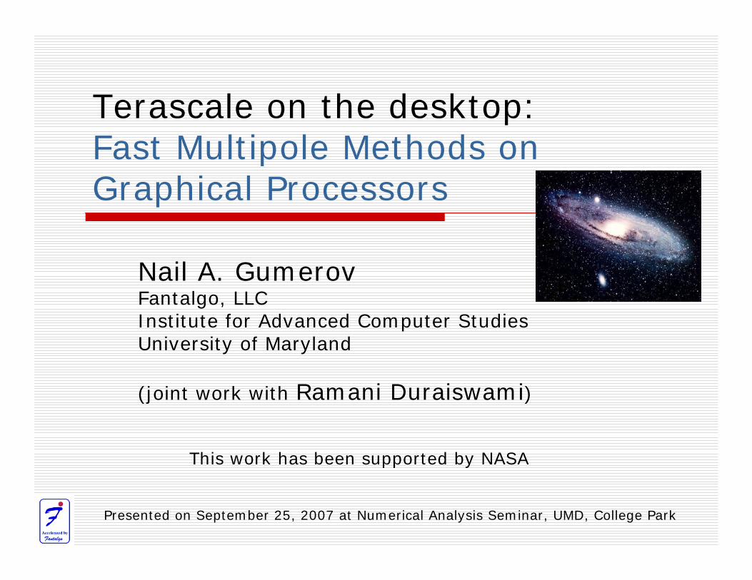
Large problems. Example 1: Sound scattering from complex shapes.

Mesh: 33082 elements16543 vertices

KEMAR Mesh:405002 elements, 202503 vertices

Problem:

Boundary value problem for the Helmholtz equation in complex 3D domain for a range of frequencies (e.g. 200 frequencies from 20 Hz to 20 kHz).

Large problems. Example 2: Stellar dynamics.

Problem:

Compute dynamics of star cluster (Solve large system of ODE’s).

Info: A galaxy like Milky Way has 100 millions stars and evolves for billions years.

Large problems. Example 3: Imaging (Medical, Geo, Weather, etc.), Computer Vision and Graphics.

Problems:

3D, 4D (and more D) interpolation of scattered data;

Discrete transforms;

Data compression and representation.

Much more…

Moore’s law

In 1965, Intel co-founder Gordon Moore saw the future. His prediction, now popularly known as Moore's Law, states that the number of transistors on a chip doubles about every two years.

Other versions:Every 18 months,Every X months.

Some other “laws”

Wirth’s law : Software is decelerating faster than hardware is accelerating.

Gates’ law: The speed of commercial software generally slows by fifty percent every 18 months.

(never formulated explicitly by Bill Gates, but rather relates to Microsoft products).

Graphical processors (GPU)

GPU RSX at 550MHz 1.8 teraflop floating point performance

Graphical processors (GPU)

NVIDIA® GeForce® 8800 GTX July 2007

500330GFLOPS

1.5 GB768 MBMemory

C870 Tesla

8800 GTX

The NVIDIA® Tesla™ C870 GPU Computing processor and D870 Deskside Supercomputer will be available in October 2007.

$500

General purpose programming on GPU (GP GPU)

ChallengesProgramming languagesNVIDIA and CUDA Math libraries (CUBLAS, CUFFT)Our middleware libraryExamples of programming using the middleware library

ChallengesSIMD (single instruction multiple data) semantics;

common algorithms should be mapped to SIMD;heavy degradation of performance for operations with structured data;optimal sizing dependent on the GPU architecture (e.g. 256 threads per block, 32n blocks, 8 processors, 16 multiprocessors);

Lack of high level language compilers and environments friendly to scientific programming;

a scientific programmer should take care on many issues on low programming level; difficult debugging;

Uncommon for scientific programming elementary computing:accuracy and error handling non-compliant with the IEEE standards;native single precision float computations;lack of many basic math functions;

Substantial difference in speeds to access different memory types; low local (cache or fast (shared)) memory;algorithms should be redesigned to take into account several different types of memory (size and access speed);

A skillful programming is needed to realize all potential of the hardware (learning, training, experience, etc.);

Programming languages

OpenGL, ActiveX, Direct3D, …;Cg;Cu.

Compute Unified Device Architecture (CUDA) of NVIDIA

Ideology:Main flow of the algorithm is realized on CPU with conventional C or C++ programming;High performance functions are implemented in Cu and precompiled to objects (analog of dynamically linked libraries);API is used to communicate with GPU:

Allocate/deallocate GPU global memory;transfer data between the GPU and CPU;manage global variables on GPU;call global functions implemented on CU;

Several high performance functions, including FFT and BLAS functions are implemented and are callable as library functions.

Math libraries (CUBLAS and CUFFT)

Callable from C, C++;CUBLAS is supplied by a Fortran wrapper;CUFFT can be also easily wrapped, e.g. to be called from Fortran.

Our middleware library(Main concepts)

Global algorithm instructions should be executed on CPU, while data should reside on GPU (minimize data exchange between the CPU and GPU);Variables allocated in global GPU memory should be transparent for CPU (easy dereferencing, access to parts of variables);Easy handling of different types, sizes, and shapes of variables;Short functions headers, similar to those in high level languages (C, Fortran);Use in full extend CUBLAS, CUFFT, and other future math libraries;Possibility for easy writing of new custom functions and including to the library.

Realization

Use structures available in C and Fortran 9x (encapsulation);Use CUDA;Wrap some CUDA and CUBLAS/CUFFT functions;Use customizable modules in Cu for easy modification of existing or writing new functions.

Example of fast “GPU’zation” of Fortran 90 subroutine using middleware library

Original fortran subroutine is from pseudospectralplasma simulation program of William Dorland

Example: Performance of a code generated using the middleware library

1.E-02

1.E-01

1.E+00

1.E+01

1.E+02

1.E+01 1.E+02 1.E+03 1.E+04N (equivalent grid (NxN))

Tim

e (s

)

y=ax2

y=bx2

a/b=25

2D MHD Simulations(100 Time Steps in Pseudospectral Method)

CPUGPU

CPU: 2.67 GHz Intel Core 2 extreme QX 7400 (2GB RAM and one of four CPUs employed).

GPU: NVIDIA GeForce8800 GTX.

Fast Multipole Method (FMM)

AboutAlgorithmData structuresTranslation theoryComplexity and optimizationsExample applications

About the FMMIntroduced by Rokhlin & Greengard (1987,1988) for computation of 2D and 3D fields for Laplace Equation;Reduces complexity of matrix-vector product from O(N2) to O(N) or O(NlogN) (depends on data structure);Hundreds of publications for various 1D, 2D, and 3D problems (Laplace, Helmholtz, Maxwell, Yukawa Potentials, etc.);We taught the first in the country course on FMM fundamentals & application at the University of Maryland (2002);Our reports on fundamentals of the FMM and lectures are available online (visit our web pages).

About the FMM

Compute matrix-vector product Some kernels

Laplace 3D:

Helmholtz 3D:

Gaussian nD:

Problem:

Major principle: Use expansions.

Theorem 1. The field of a single source located at x0 can be locally expanded about center x* into absolutely and uniformly convergent series in domain |y-x*|<r<R<|x0 -x*| (local, or R-expansion).

Corollary: holds for the field of s sources located outside the sphere |xi-x*|>R.

Theorem 2: The field of a single source located at x0 can be expanded about center x* into absolutely and uniformly convergent series in domain |y-x*|>R>r>|x0 -x*| (multipole, or S-expansion).

Corrolary: holds for the field of s sources located inside the sphere |xi -x*|<r.

Theorem 3: R- and S-expansions can be translated (change of the basis and/or the expansion center, subject to geometric constraints).

E.g. for Laplace kernel:

FMM algorithm

xixc(n,L)

y

Upward pass (get S-expansions for all boxes (skip empty))(S-expansion means singular, or multipole, or far field expansion)

Computational domain (nD cube) is partitioned by quadtree (2D) or octree (3D).

1. Get S-exp for Max Level2. Get S-exp for other levels(use S|S-translations)

FMM algorithmDownward pass (get R-expansions for all boxes (skip empty))(R-expansion means regular, or local, or near field expansion)

1. Get R-exp from S-exp’sof the boxes in the neighborhood(use S|R-translations)

2. Get R-exp from parent(use R|R-translations)

FMM algorithmFinal evaluation (evaluate R-expansions for boxes at Max Level)and sum up directly contributions of sources in the neighborhoodof receivers )

1. Evaluate R-exp 2. Direct summation

yj yj

Data structuresBinary, quad- or octrees (1,2, and 3D);Determines MaxLevel based on clustering parameter;Requires building of lists of neighbors and neighborhood data structure (e.g. for fast determination of boxes in the neighborhood of the parent box);Requires indexing of sources and receivers in boxes;We do all this on serial CPU using bit interleaving technique, sorting, and operations on sets (union, intersection, etc.);Overall complexity of our algorithm O(NlogN);Normally the complexity of generation of data structure is lower than for the run part of the algorithm;Additional amortization: in many problems the data structure should be set once, while the run part can be executed many times (iterative solution of linear system);It is a non-trivial task to parallelize this algorithm while we expect to perform this task in closest future.

Translation theoryStandard translation method: Apply p2 x p2 matrix to p2 vector of expansion coefficients: O(p4) complexity;There exist O(p3) methods:

Currently we use the RCR-decomposition of the translation operators (Rotation-Coaxial Translation-Back Rotation);Sparse matrix decomposition (a bit slower, but less local memory);

There exist O(p2) or O(p2logp) methods based on diagonal forms of translation operators:

Greengard-Rokhlin exponential forms for truncated conical domain (require some O(p3) transforms);FFT-based methods (large asymptotic constants);Our own O(p2 ) diagonal form method (problems with numerical stability, especially for single precision);Diagonal forms require larger function representations (samplings on grid) than spectral expansions, and effective asymptotic constants are larger than for the RCR);

For relatively low p, which is sufficient for single precision (p=4,…,12), the RCR-method is comparable in speed with the fastest O(p2) methods.

Translation theory (RCR-decomposition)

z

y

y

xx

yx

z

yx

z

zp4

p3p3

p3

z

y

y

xx

yx

zyx

z

yx

z

zp4

p3p3

p3

From the group theory follows that general translation can be reduced to

Translation theory Reduction of translation complexity by using translation stencils and variable truncation number:

e.g. S-expansions from the shaded boxes can be translated to the center of the parent box, with the same error bound as from the white box to the child.

Also for each box its own truncation number can be used.

Complexity of the FMM

Operations, which do not depend on the number of boxes:(Generation of S-expansions and evaluation of R-expansions)Complexity: ~ AN (assume that the number of sources and receivers is of the same order).

Translation operations, which do not depend on the number of sources/receivers (only on the number of boxes)Complexity: BNboxes ~ BN/s (s is the clustering parameter).

Direct summation, depends on the number of sources/receivers and the number of sources in the neighborhood of receivers.Complexity: ~ CNs.

Total complexity: Cost = Costexp+Costtrans+Costdir~ AN+BN/s+CNs.

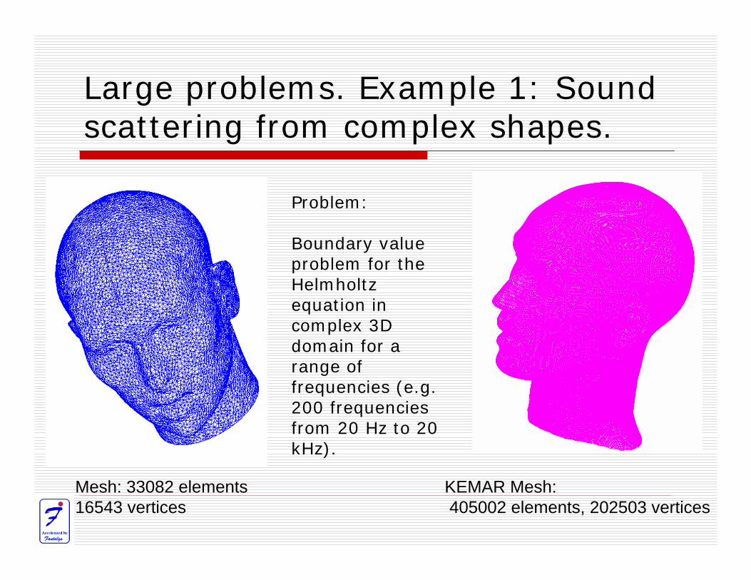
Optimization of the FMM

Total complexity: Cost(s)=AN+BN/s+CNs.

sopt = (B/C)1/2.

Optimal Max Level of the octree: lmax = log8 (N/sopt)

(Uniform distributions):

Example Applications

1000 randomly oriented ellipsoids488,000 vertices

and 972,000 elements

Potential

external Dirichlet and Neumann problems

Boundary Element Methodaccelerated by GMRES/FMMsolver


1.E-02

1.E-01

1.E+00

1.E+01

1.E+02

1.E+03

1.E+04

1.E+02 1.E+03 1.E+04 1.E+05 1.E+06Number of Vertices, N

Tota

l CP

U ti

me

(s)

GMRES+FMM

GMRES+Low Mem Direct

GMRES+High Mem Direct

LU-decomposition

O(N2) Memory Threshold

y=ax

y=bx2

y=cx3

BEMDirichlet Problemfor Ellipsoids(3D Laplace)

FMM: p = 8


1.E-03

1.E-02

1.E-01

1.E+00

1.E+01

1.E+02

1.E+02 1.E+03 1.E+04 1.E+05 1.E+06

Number of Vertices, N

Sing

le M

atrix

-Vec

tor M

ultip

licat

ion

CPU

Tim

e (s

)

y=ax

y=bx2Number of GMRES Iterations

FMM

Direct+Matrix EntriesComputation

Multiplicationof Stored Matrix

3D Laplace FMM: p = 8


kD=0.96 kD=9.6 kD=96(250 Hz)

Sound pressure

(2.5 kHz) (25 kHz)

BEM for the Helmholtz equation (fGMRES/FMM)Mesh: 132,072 elements, 65,539 vertices

FMM on GPU

Challenges Effect of GPU architecture on FMM complexity and optimizationAccuracy Performance

Challenges

Complex FMM data structure; Problem is not native for SIMD semantics;

non-uniformity of data causes problems with efficient work load (taking into account large number of threads);serial algorithms use recursive computations;existing libraries (CUBLAS) and middleware approach are not sufficient;high performing FMM functions should be redesigned and written in CU;

Low fast (shared/constant) memory for efficient implementation of translation operators;Absence of good debugging tools for GPU.

High performance direct summation on GPU (total)

1.E-04

1.E-03

1.E-02

1.E-01

1.E+00

1.E+01

1.E+02

1.E+03

1.E+04

1.E+03 1.E+04 1.E+05 1.E+06Number of Sources

Tim

e (s

)

y=ax2

y=bx2CPU, Direct

GPU, Direct

3D Laplace

y=bx2+cx+d b/a=600CPU direct:

serial code;no use of partial caching;no loop unrolling;

(simple execution of nested loop)

Computations of potentialCPU: 2.67 GHz Intel Core 2 extreme QX 7400 (2GB RAM and one of four CPUs employed).

GPU: NVIDIA GeForce8800 GTX (peak 330 GFLOPS).

Estimated achieved rate:190 GFLOPS.

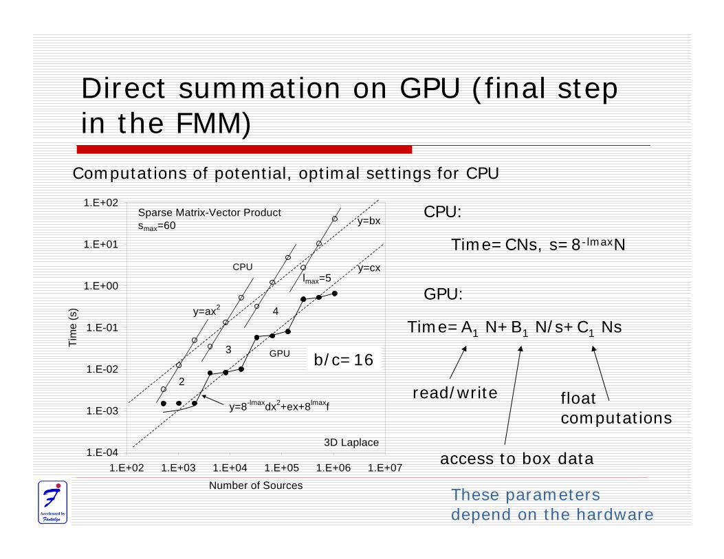
Direct summation on GPU (final step in the FMM)

Computations of potential, optimal settings for CPU

1.E-04

1.E-03

1.E-02

1.E-01

1.E+00

1.E+01

1.E+02

1.E+02 1.E+03 1.E+04 1.E+05 1.E+06 1.E+07Number of Sources

Tim

e (s

) y=ax2

y=cx

GPU

3D Laplace

y=8-lmaxdx2+ex+8lmaxf

CPU

Sparse Matrix-Vector Productsmax=60 y=bx

2

3

4

lmax=5

b/c=16

Time=CNs, s=8-lmaxN

CPU:

GPU:

Time=A1 N+B1 N/s+C1 Ns

read/write

access to box data

float computations

b/c=16

These parameters depend on the hardware


Cost =A1 N+B1 N/s+C1 Ns.

Compare GPU final summation complexity:

and total FMM complexity:

Cost = AN+BN/s+CNs.

sopt = (B1 /C1 )1/2,

Optimal cluster size for direct summation step of the FMM

and this can be only increased for the full algorithm, since its complexity

Cost =(A+A1 )N+(B+B1 )N/s+C1 Ns,

and sopt = ((B+B1 )/C1 )1/2.


Computations of potential, optimal settings for GPU

1.E-04

1.E-03

1.E-02

1.E-01

1.E+00

1.E+01

1.E+02

1.E+03

1.E+03 1.E+04 1.E+05 1.E+06 1.E+07Number of Sources

Tim

e (s

)

y=ax2

y=cx

GPU

3D Laplace

y=8-lmaxdx2+ex+8lmaxf

CPU

Sparse Matrix-Vector Productsmax=320 y=bx

2

3

lmax=4

b/c=300b/c=300


Computations of potential, optimal settings for CPU and GPU

N Serial CPU (s) GPU(s) Time Ratio

4096 3.51E-02 1.50E-03 23 8192 1.34E-01 2.96E-03 45 16384 5.26E-01 7.50E-03 70 32768 3.22E-01 1.51E-02 21 65536 1.23E+00 2.75E-02 45 131072 4.81E+00 7.13E-02 68 262144 2.75E+00 1.20E-01 23 524288 1.05E+01 2.21E-01 47 1048576 4.10E+01 5.96E-01 69

Important conclusion:

Since the optimal max level of the octreewhen using GPU is lesser than that for the CPU, the importance of optimization of translation subroutines diminishes.

Other steps of the FMM on GPU

Accelerations in range 5-60;Effective accelerations for N=1,048,576 (taking into account max level reduction): 30-60.

Accuracy

Relative L2 –norm error measure:

CPU single precision direct summation was taken as “exact”;100 sampling points were used.

What is more accurate for solution of large problems on GPU: direct summation or FMM?

1.E-09

1.E-08

1.E-07

1.E-06

1.E-05

1.E-04

1.E-03

1.E-02

1.E+02 1.E+03 1.E+04 1.E+05 1.E+06 1.E+07Number of Sources

L2-r

elat

ive

erro

r

p=4

p=8

p=12

Direct

CPU

GPU

FMM

FMM

FMM

Filled = GPU, Empty = CPU

Error in computations of potential Error computedover a grid of 729 sampling points, relative to “exact”solution, which is direct summation with double precision.

Possible reason why the GPU error in direct summation grows: systematic roundofferror in computation of function 1/sqrt(x).(still a question).

Performance

661.761 s116.1 sp=12

721.227 s88.09 sp=8

290.979 s28.37 sp=4

RatioGPUserial CPU

(potential only)N=1,048,576

481.395 s66.56 sp=12

560.908 s51.17 sp=8

330.683 s22.25 sp=4

RatioGPUserial CPU

(potential+forces (gradient))N=1,048,576

Performance

1.E-03

1.E-02

1.E-01

1.E+00

1.E+01

1.E+02


Run

Tim

e (s

)

y=ax2y=bx2

y=cx

y=dx

CPU, Direct

GPU, DirectCPU, FMM

GPU, FMM

3D Laplace

a/b = 600c/d = 50

p=8, FMM error ~ 10-5

1.E-03

1.E-02

1.E-01

1.E+00

1.E+01

1.E+02


Run

Tim

e (s

)

y=ax2

y=bx2

y=cx

y=dx

CPU, Direct

GPU, Direct

CPU, FMM

GPU, FMM

3D Laplace

a/b = 600c/d = 50

p=12, FMM error ~ 10-6

1.E-03

1.E-02

1.E-01

1.E+00

1.E+01

1.E+02


Run

Tim

e (s

)

y=ax2 y=bx2

y=cx

y=dx

CPU, Direct

GPU, Direct

CPU, FMM

GPU, FMM

3D Laplace

a/b = 600c/d = 30

p=4, FMM error ~ 2·10-4

p=4 p=8 p=12

Performance

Computations of the potential and forces:

Peak performance of GPU for direct summation 290 Gigaflops, while for the FMM on GPU effective rates in range 25-50 Teraflops are observed (following the citation below).

M.S. Warren, J.K. Salmon, D.J. Becker, M.P. Goda, T. Sterling & G.S. Winckelmans. “Pentium Pro inside: I. a treecode at 430 Gigaflops on ASCI Red,” Bell price winning paper at SC’97, 1997.

CPU

GPU

direct

dir

FMM

FMM

Conclusions

What do we haveWhat is next

What do we have

Some insight and methods of programming on GPU;High performance FMM for 3D Laplace kernel running in configuration 1CPU-1GPU;Results encouraging to continue.

What is next

Applications of the FMM matrix-vector multiplier for solution of physics-based and engineering problems (particle/molecular dynamics, boundary element methods, RBF interpolation, etc.);Mapping on GPU algorithms generating FMM data structures;Develop the FMM for larger CPU/GPU clusters and hit “big”problems;Some research to adjust the algorithms for GPU, particularly more efficient use of shared/constant memory;FMM on GPU for different kernels (we see a lot of applications);Continue to work towards simplification of programming on GPU for scientists;Upgrades in hardware (double precision, larger memory, etc.) areexpected.

Thank you !

OutlineIntroduction

Large computational tasksMoore’s lawGraphical processors (GPU)

General purpose programming on GPUChallengesNVIDIA and CUDA Math libraries (CUBLAS, CUFFT)Middleware libraries

Fast Multipole Method (FMM)AlgorithmData structuresTranslation theoryComplexity and optimizations

FMM on GPUChallengesEffect of GPU architecture on FMM complexity and optimizationAccuracyPerformance

ConclusionsWhat do we haveWhat is next

Terascale on the desktop: Fast Multipole Methods on ... · Fast Multipole Methods on Graphical...

Documents

Transcript of Terascale on the desktop: Fast Multipole Methods on ... · Fast Multipole Methods on Graphical...