Prepared for submission to JHEP

Tensor network and (p-adic) AdS/CFT

Arpan Bhattacharyyaa, Ling-Yan Hunga,b,c, Yang Leid, and Wei Lid

a Department of Physics and Center for Field Theory and Particle Physics, Fudan Uni-

versity,

220 Handan Road, 200433 Shanghai, P. R. Chinab State Key Laboratory of Surface Physics and Department of Physics, Fudan University,

220 Handan Road, 200433 Shanghai, P. R. Chinac Collaborative Innovation Center of Advanced Microstructures, Nanjing University,

Nanjing, 210093, P. R. China.d CAS Key Laboratory of Theoretical Physics, Institute of Theoretical Physics,

Chinese Academy of Sciences, 100190 Beijing, P.R. China

E-mail: bhattacharyya.arpan@yahoo.com,

elektron.janethung@gmail.com, yanglei@itp.ac.cn,

weili@itp.ac.cn

Abstract: We use the tensor network living on the Bruhat-Tits tree to give a

concrete realization of the recently proposed p-adic AdS/CFT correspondence (a

holographic duality based on the p-adic number field Qp). Instead of assuming the

p-adic AdS/CFT correspondence, we show how important features of AdS/CFT such

as the bulk operator reconstruction and the holographic computation of boundary

correlators are automatically implemented in this tensor network.

arX

iv:1

703.

0544

5v3

[he

p-th

] 2

5 Ja

n 20

18

Contents

1 Introduction 1

2 Short review of tensor networks 4

2.1 Tensor network as ansatz for N -body wavefunction 4

2.2 Tensor network as discrete holographic correspondence 5

2.2.1 Bulk and boundary in tensor networks 6

2.2.2 Perfect tensor code and operator pushing 7

2.3 Some open questions in tensor network as discrete AdS/CFT 8

3 Bulk operator reconstruction 9

3.1 From HKLL to operator pushing 9

3.2 Operator pushing 10

3.2.1 Local operator pushing 10

3.2.2 Global operator pushing 13

3.3 Linear order in HKLL 13

3.4 Non-linear orders in HKLL 15

4 Tensor networks on p-adic tree 16

4.1 From tessellation to tree 16

4.1.1 Limitation of tensor networks based on regular tessellation 16

4.1.2 Tensor networks on abstract tree 18

4.2 p-adic number field and Bruhat-Tits tree 18

4.2.1 The field Qp of p-adic numbers 19

4.2.2 Bruhat-Tits tree as bulk of p-adic line Qp 20

4.3 Conformal primaries for tensor network on Bruhat-Tits tree 22

4.3.1 SL(2,Qp) action on Bruhat-Tits tree 22

4.3.2 Choice of cutoff surface 23

4.3.3 Conformal primaries for p-adic tensor network 24

5 p-adic HKLL from tree tensor networks 26

5.1 HKLL for tree tensor network 26

5.2 p-adic HKLL 28

5.2.1 Reconstruction kernel v.s. propagator 28

5.2.2 Reconstruction kernel in terms of p-adic variables 29

5.3 Linear term of HKLL as wavelet transform 30

5.3.1 Wavelet review 30

5.3.2 Real linear HKLL as real wavelet 31

5.3.3 p-adic linear HKLL as p-adic wavelet 33

– i –

6 Correlation functions and emergent Witten diagrams 36

6.1 Constructing conformal primaries in p-adic tensor network 36

6.2 Two-point functions 38

6.3 Higher point functions 39

6.4 Conformal primaries basis v.s. operator pushing basis 40

7 Summary and Discussion 42

7.1 Implication to p-adic AdS/CFT 44

7.2 Further explorations in tensor networks 45

A Lattice construction of Bruhat-Tits tree 47

B Basics of p-adic analysis 49

B.1 p-adic integration 49

B.2 p-adic Fourier transform 50

C Some examples 51

C.1 GHZ tensor 51

C.2 Random tensors 52

D Bulk operator reconstruction in the vicinity of the perfect code 53

E Boundary global Space (time) symmetry via tensor transforma-

tions 53

E.1 Example using the 3-qutrit code 54

1 Introduction

The principle of holographic duality states that quantum gravity in a spacetimeM is

equivalent to a quantum field theory on the boundary ∂M [1, 2]. Both conceptually

and mathematically, it provides one of the most powerful tools to understand non-

perturbative quantum gravity (via its dual quantum field theory description). The

most prominent and tractable holographic duality arises when the spacetime is anti-

de Sitter (AdS), where we have the AdS/CFT correspondence [3]: quantum gravity

in an asymptotically AdS spacetime is equivalent to a conformal field theory (CFT)

living on the boundary of the AdS spacetime.

While the duality was first engineered from string theory, the Area Law of black

holes and general arguments based on the entropy bound suggest that the holographic

principle is independent from string theory [1, 2]. How to understand holographic

– 1 –

dualities independent of the string theory framework? What is the underlying mecha-

nism of AdS/CFT? Proving AdS/CFT would be very difficult because (in most of its

parameter regime) it is a strong/weak duality. However, short of proving AdS/CFT,

is it at least possible to see it emerge from some constructions (other than string

theory), i.e. without inputing it as an assumption?

Above is the background motivation of the current work. Based on the holo-

graphic entropy formula by Ryu and Takayanagi, it was noticed by Swingle that

certain types of tensor networks can have features of a holographic correspondence

[5]. The observation stimulated a surge of investigations [6–26] on various other types

of tensor networks and there is increasing evidence that tensor networks can capture

essential features of AdS/CFT.

An important recent development is the proposal of the holographic code based

on perfect tensors on a network embedded in a negatively-curved space [19],1 which

recovers the RT formula naturally and exhibits the causality that mimics an error

correcting code. Perturbing away from perfect tensors, other features of AdS/CFT,

such as structures similar to Witten diagrams in the computation of correlation

functions, also emerge [21].

To further proceed, the study of holographic tensor networks needs to address

some conceptual questions. A tensor network lives on a discrete space. To which

extent can it capture the AdS/CFT correspondence, which has only been defined

for continuous spacetimes? Does there exist a discrete version of the AdS/CFT

correspondence which tensor networks can capture fully?

To answer these questions, in this paper we try to realize the following two impor-

tant aspects of holography in tensor networks: (1) reconstruction of bulk operators

and (2) holographic computation of boundary correlators.

There are two main differences from previous studies of holographic tensor net-

works. First of all, we use rather generic tensors. The restriction to perfect tensors

in [19] makes it easy to do explicit computations in tensor networks. However it was

later found that in order to have non-trivial correlation functions we need to use

imperfect tensors [21].

Second, we propose to put the tensor network on the Bruhat-Tits (BT) tree,

which is a geometrical presentation of the p-adic expansion of a p-adic number.

Thus far, the lack of symmetry has been a bottleneck in the development of tensor

networks.2 The main problem is that if we assume that the tensor network realizes

a “naive” discretization of the AdS space, i.e. that the tensor network lives on the

(dual graph) of a regular tiling of AdS, then the presence of the lattice breaks the

continuous isometry group (e.g. SL(2,R) in a 2D bulk) down to a discrete subgroup

1Perfect tensors emerge very naturally in spaces of tensors with large bond dimensions [20].2See however [21] that initiated the study on symmetries in the tensor network.

– 2 –

of the isometry of AdS. The discrete subgroups preserved by these regular tilings

are Coxeter groups, whose representation theory, to our knowledge, is not yet strong

enough to give a good description of eigenfunctions on the graph.

To gain more symmetry and quantitative control of the graph wavefunctions, we

instead look at tensor networks living on the Bruhat-Tits tree. The Bruhat-Tits tree

preserves the full conformal group SL(2,Qp) — only with the real field R replaced

by a different field completion Qp of the rational numbers. This is a continuous

group, and hence much larger than the discrete subgroup of SL(2,R) preserved by

any regular tessellation of the AdS space. Therefore a tensor network based on the

Bruhat-Tits tree would have much more symmetry than its counterpart living on a

regular tessellation.

This is inspired by recent proposals for the p-adic AdS/CFT correspondence [26–

28], which generalize the AdS/CFT dictionary to the situation where the boundary

theory lives on a space-time that is based on the field Qp (which is continuous), and

where the discrete BT tree plays the role of the bulk AdS space.3 Besides being an

interesting holographic duality that is based on Qp instead of R, p-adic AdS/CFT

might also become relevant to the analysis of the continuous version via the adelic

construction.

In this paper we propose to use tensor networks to give concrete realizations of

p-adic AdS/CFT, in some sense analogous to using various D-brane configurations to

engineer corresponding AdS/CFT dualities explicitly. This is in contrast to [26, 27],

which assumed a p-adic AdS/CFT correspondence and then derived various conse-

quences. In our tensor network construction, we do not assume p-adic AdS/CFT,

but aspects of the AdS/CFT correspondence emerge from the tensor network.

A possible connection between p-adic AdS/CFT and tensor networks was first

studied in [26], whose construction is based on perfect tensors and on embedding

the Bruhat-Tits tree in the geometric tiling (in particular, the HAPPY tiling) of

the bulk. The construction in the current paper is different in that (1) we are not

using perfect tensors, building on earlier work that imperfect tensors are necessary

to furnish non-trivial correlation functions [21]; and (2) we view the Bruhat-Tits tree

as an abstract tree, and hence do not need to embed the Bruhat-Tits tree in a real

bulk space. Namely, the bulk in p-adic AdS/CFT is just the Bruhat-Tits tree itself,

and the relation to the real AdS/CFT will not come about by a naive geometric

embedding.

The paper is organized as follows. In Section 2 we review the basics of tensor

networks, in particular the intuition behind their role as a discrete holographic corre-

spondence. In Section 3 we generalize the operator-pushing technique developed for

3The discussion is mainly based on a two-dimensional bulk and a one-dimensional boundary.

The proposed higher-dimensional generalization involves finite algebraic extensions of Qp, for more

details see [26, 27].

– 3 –

perfect tensors in [19] to generic tensors, and then use it to derive a tensor network

analogue of the bulk reconstruction formula.

For generic tensor networks, the results of Section 3 lack conceptual power be-

cause to relate to AdS/CFT we need a notion of conformal or at least scaling pri-

maries. Hence in Section 4 we motivate our proposal of studying tensor networks

living on the Bruhat-Tits tree, and show that this allows us to define conformal

primaries on tensor networks.

Building on this, in Section 5 we show that the bulk reconstruction for tree tensor

networks gives a nice p-adic bulk reconstruction (i.e. HKLL) formula. We also show

a strong parallel between the real and p-adic HKLL formulae and in particular that

they can both be understood in the linear order as wavelet transforms. Section 6

computes p-adic correlations functions via tensor networks and shows how Witten

diagrams emerge in the bulk of the tensor network. Finally in Section 7 we summarize

and discuss open questions.

We leave some review and detailed computation to five Appendices. Appendix

A reviews the lattice construction of the Bruhat-Tits tree and Appendix B reviews

the basics of p-adic analysis. In Appendix C we give two explicit examples. Ap-

pendix D contains the proof of an argument for the necessity of going beyond perfect

tensors. Appendix E explains how to realize spacetime symmetry via tensor network

transformations.

2 Short review of tensor networks

In this section we first review basic aspects of tensor networks to fix notations.4 We

then explain the intuition behind attempts at using them to realize discrete versions

of the holographic duality [19, 20]. Finally we discuss open questions in tensor

networks that motivated this work.

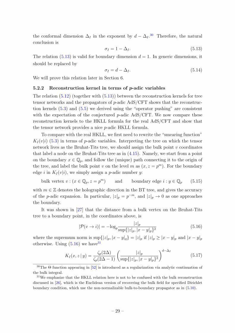
2.1 Tensor network as ansatz for N -body wavefunction

Solving for exact wavefunctions |ψ〉 of a quantum many-body system analytically is

in general a very difficult problem, because of the gigantic dimension of the Hilbert

space. Consider a N -body Hamiltonian H. Generically, its wavefunction |ψ〉 is given

by a rank-N tensor:

|ψ〉 =∑i1···iN

fi1···iN |i1 · · · iN〉 (2.1)

for 1 ≤ ik ≤ D, where D is the dimension of the Hilbert space at each site.5 De-

termining the wavefunction |ψ〉 would therefore involve solving for DN numbers of

unknowns, which scales exponentially with N .

4For a good review on tensor networks see [29, 30].5We have assumed that the full Hilbert space of the N -body system can be factorized into direct

products of Hilbert spaces on each site H = ⊗Ni=1Hi.

– 4 –

The tensor network was introduced as a “clever” ansatz for |ψ〉 that can greatly

simplify the above problem. In this ansatz, the rank-N tensor fi1···iN in the original

wavefunction |ψ〉 is decomposed into many much smaller tensors T (v) (with rank-rv)

contracted together:

fi1···iN =∑µ1,µ2···

Ti1··· ;µ1µ2···(1)Tik··· ;µ1µ3···(2) · · · . (2.2)

In the r.h.s. the original indices from i1 to iN remain un-contracted and we will call

them physical or external indices, and µn denotes internal indices that are contracted

between tensors.

The contraction of internal indices in the ansatz (2.2) can be better presented

graphically — in terms of a connected graph G (or “network”), where each tensor

T (v) (with rank-rv) is represented by a vertex v with valency rv, each contracted

index µn by an edge between two vertices, and each physical index ik by an external

leg at the boundary of G.

One can immediately see that the ansatz (2.2) can greatly simplify the problem

by counting the number of degrees of freedom in the r.h.s. of (2.2). For a network

consisting of M vertices, and for simplicity assuming that they all have the same

valency r, the number of total degrees of freedom is then MDr. Since in a typical

tensor network, M ∼ O(Nd) — here d is a small number that depends on the

spacetime dimension and the choice of network — whereas r ∼ O(1), the tensor

network ansatz has far fewer degrees of freedom than the original N -body problem:

DN �MDr. (2.3)

One can then numerically solve for the ground state wavefunction |ψ〉 by minimizing

the energy 〈ψ|H|ψ〉.What makes a particular tensor network ansatz (2.2) numerically efficient and yet

remains a good approximation is that the network G needs to be chosen according

to the quantum entanglement structure of the given N -body system. Figure [1]

shows three well-studied tensor network ansatze, according to three different types

of entanglement structures.

2.2 Tensor network as discrete holographic correspondence

What makes tensor network more than a good computational tool in many-body

systems is the realization that certain types of tensor networks can have features of

a holographic correspondence. This was realized by Swingle in 2011 [5], for the case

of the MERA (multi-scale entanglement renormalization ansatz) network.

In the MERA network shown in Figure 1-(b), the physical legs are at the bottom

of the network. Moving upwards in the network are alternating layers of 4-valent

– 5 –

Figure 1. Three well-studied tensor networks. (a) Matrix Product State for (1+1)-dim

gapped systems. (b) MERA network for in (1+1)-dim gapless systems. (c) Projected

Entangled Pair States for (2+1)-dim systems. Picture courtesy of [29].

vertices (disentanglers) and those with 3-valent vertices (isometries).6 Each set of

these twin layers serves as a linear map that projects the system to a coarse-grained

one (hence the “renormalization” in the name). As one moves up the graph, a new

scale, i.e. an extra dimension, emerges, which is very similar to AdS/CFT in which

the radial direction of the AdS bulk plays the role of the RG scale.

Moreover, the entanglement entropy of the MERA network is bounded from above

[5] by the length of the geodesic cutting through the network, reminiscent of the Ryu-

Takayanagi formula that computes the entanglement entropy via holography [31, 32].

2.2.1 Bulk and boundary in tensor networks

To establish a more concrete connection between tensor networks and holography,

let’s first define the meaning of bulk and boundary in the context of tensor networks.

The network G plays the role of the (discrete) bulk space. The bulk Hilbert space

is defined as follows. First, assign a D-dim Hilbert space He to each edge,7 and a

Dr-dim Hilbert space Hv ≡ ⊗re(v)=1He(v) to each vertex v. (Here e(v) denotes an

edge emitting from vertex v.) The tensor T (v) then essentially defines a state in Hv

|T (v)〉 ≡∑{ai}

Ta1···ar(v)|a1 · · · ar〉. (2.4)

The bulk Hilbert space is then

Hbulk ≡ ⊗Mv=1Hv, (2.5)

6Without disentanglers, the MERA network reduces to a tree, which (in this naive setting)

cannot reproduce the entanglement structure of a gapless system that the MERA network wants

to describe.7We assume that the bond dimension D for each edge, i.e. the size of each He, is the same.

– 6 –

where M is the total number of vertices in the network. A generic bulk state is then

|Ψbulk〉 =∑{T (v)}

α{T (v)} (⊗v|T (v)〉) . (2.6)

In the simplest case (as in section 2.1), it is a product state |Ψbulk〉 = ⊗v|T (v)〉.The boundary Hilbert space is just the original H defined at the beginning of

this section:

Hbndy = ⊗Ni=1Hi, (2.7)

where Hi is the Hilbert space living on the external leg i of the network G.

The map from bulk to boundary is via a projection operator that effectively

contracts all the internal indices:

|ψbndy〉 = (⊗all internal edges µ|µ〉〈µ|) |Ψbulk〉. (2.8)

For each internal edge µ (connecting two vertices v and w), |µ〉 is defined as

|µ〉 ≡ |µv,w〉 =∑

αµv ,ανw

καµvανw |αµv〉 ⊗ |ανw〉, (2.9)

where |αµv〉 denotes the state located at the edge-µ of the vertex v. The boundary

wavefunction is thus defined by projecting the edges connecting two vertices into an

entangled state. In most cases considered, such as our example described in (2.2)

and in the rest of the paper, the “metric” καµvανw = δαµvανw .

2.2.2 Perfect tensor code and operator pushing

An important shortcoming of the MERA network as discrete holography is that

the Ryu-Takayanagi formula does not compute its entanglement entropy but only

provides an upper bound. Part of the reason is that its network does not preserve

enough of the hyperbolic isometries expected for the dual theory of a CFT.

The “HAPPY” code in [19] improved this by choosing the network G to be

the dual graph of a regular tessellation of the hyperbolic space. With the further

assumption that the tensors are restricted to be “Perfect Tensors”, the HAPPY code

was the first tensor network that exactly recovers the Ryu-Takayanagi formula [19].

The restriction to “Perfect tensors” greatly simplifies the derivation in [19]. They

are even-rank tensors with the following property: for any partition of the r indices

into two sets n ∈ {µ1, . . . µk} and a ∈ {µk+1, . . . µr} with k ≤ r2, Tna is a norm-

preserving projection operator from a to n:

TnaT†an′ = D

r2−k δnn′ . (2.10)

In particular, when k = r2, Tna becomes a unitary map: TnaT

†an′ = δnn′ .

– 7 –

Another important result in [19] is the exhibition of the causal structure in the

HAPPY code: it was shown that a operator acting on the bulk of the HAPPY

code can be recovered using only boundary operators that act on a subregion of the

boundary.8

This was shown using the method of “operator pushing”, invented for the perfect

tensor by [19]. Let’s illustrate this method with a particular example of a perfect

tensor code: the hexagon code (i.e. r=6) with bond dimension D = 2.

A tensor state |T 〉 in the hexagon code is invariant under a set of 6 stabilizers

S(a):

S(a)|T 〉hexagon = |T 〉hexagon a = 1, 2, . . . , 6. (2.11)

Since D = 2, S(a) can be expressed in terms of Pauli matrices {X, Y, Z} acting on

the 6 edges. We can choose a basis such that9

S(1) = X1 ⊗X2 ⊗X3 ⊗X4 ⊗X5 ⊗X6 etc (2.12)

where Xi acts on the ith leg of |T 〉. We immediately see that (2.11) with the stabilizer

(2.12) implies

∀v : Xi|T 〉hexagon = ⊗j 6=iXj|T 〉hexagon (2.13)

Namely, applying the operator X one of the legs of |T 〉 is equivalent to applying X

on the other five legs.

Applying other stabilizers gives similar “operator pushing” rules, in which an

operator acting on a given leg of a bulk tensor site can be “pushed” to the other legs

of the same site. Applying the set of rules repeatedly, one can move the effect of a

bulk operator all the way to the boundary, using which [19] showed the emergence

of the causal structure in the perfect tensor code. The main idea can be generalized

to general tensors and will be used later to derive the tensor network analogue of the

HKLL formula.

2.3 Some open questions in tensor network as discrete AdS/CFT

For tensor networks to realize a discrete version of AdS/CFT, the following aspects

need to be further developed.

1. Global symmetries of the boundary wavefunction v.s. isometries of the network.

In traditional AdS/CFT, gauge symmetries of the bulk are mapped to global

symmetries of the boundary theory. In particular, the isometries of the bulk

spacetime are mapped to global spacetime symmetries of the boundary CFT.

8This is analogous to the bulk operator in the Rindler coordinates, in which only the subregion

within the causal wedge containing the original bulk operator is involved.9For the full list of stabilizers see [19].

– 8 –

How to realize the interplay between bulk isometries and boundary global sym-

metries in the tensor network? Further, how to effectively use the symmetry

in the tensor network computation to model discrete AdS?10

2. Going beyond perfect tensors

Though greatly simplifying the computation, perfect tensors are in some sense

“too perfect” — namely too symmetric to allow enough dynamical content.

For example, in a tensor network with only perfect tensors there exists no

connected correlation function between local operators [21].

3. Tensor network analogue of the HKLL formula

As we demonstrate in Appendix E, in a tensor network using perfect tensors, a

bulk operator can be reconstructed only as macroscopic products of boundary

operators. This is in sharp contrast with the HKLL formula where in the large

N limit, the leading contribution is linear in the boundary operators. We need

to generalize the operator-pushing technique invented for perfect tensors to

more generic tensors, and find a tensor network analogue of the HKLL formula.

In this paper, we will take some further steps in clarifying these questions.

3 Bulk operator reconstruction

In this section we show how the bulk operator reconstruction is realized tensor net-

works. This was initiated for the special case of perfect tensors in [19]. We first

show that in order to have the analogue of the HKLL formula one needs to use more

general tensors, then derive an analogue of the HKLL formula for tensor networks.

3.1 From HKLL to operator pushing

In AdS/CFT, a normalizable local field in the bulk φI(~x, z) can be reconstructed

from the boundary operators via the HKLL formula [34, 35]11

φI(~x, z) =

∫ddy KI( ~x, z |~y )OI(~y)

+∑J,K

λIJKN

∫ddx′dz′GI(~x, z|~x′, z′)

∫ddy1KJ(~x′, z′|~y1)OJ(~y1)

∫ddy2KK(~x′, z′|~y2)OK(~y2)

+O(λ2

N2)

∫. . .

(3.1)

10Some discussion on how tensor networks reproduce such features already appeared in [33].11Here (~x, z) denotes the Poincare coordinate with the metric ds2 = 1

z2 (dz2 + d~x2) and ~x is the

boundary d-vector with ~x2 ≡ ηµνxµxν with negative signature.

– 9 –

where OI is the boundary operator that is dual to the bulk field φI : limz→0 φI(~x, z) =

z−∆IOI(~x) (with ∆I the conformal dimension ofOI). HereKI( ~x, z |~y ) is the boundary-

bulk kernel (called “smearing function” here) of OI :

KI(~x, z | ~y ) =

(z

z2 − (~x− ~y)2

)d−∆I

Θ(z2 − (~x− ~y)2) (3.2)

and GI(~x, z|~x′, z′) its bulk-bulk kernel. The “smearing function” and the bulk-bulk

kernel are simply related by limz′→0 z′∆I−dGI(~x, z|~x′, z′) ∼ KI(~x, z | ~x′ ). Note that

the bulk-bulk kernel here satisfies a different boundary condition from the usual bulk

propagator.

For a tensor network to be a (discrete version) of the holographic duality (3.1),

it needs to realize an analogue of the HKLL formula, i.e. an operator acting on the

|Ψbulk〉 should be reconstructed by operators acting on the |ψbndy〉, in a way similar

to (3.1). In particular, it should exhibit the causal structure (i.e. the reconstruction

should be possible using only a subregion) and an expansion in which the linear term

dominates in the large-N limit.

The emergence of the causal structure in tensor networks was realized by [19] for

a specific tensor network with “perfect tensors”. Motivated by the observation by [13]

that the causal structure in the HKLL formula (3.1) resembles the error correction

code, [19] showed that a bulk operator in the perfect code can be recovered using

only those boundary operators that live on the subregion that is causally connected

to the original bulk operator.

However, in a network with perfect tensors, a bulk operator can be reconstructed

only as a macroscopic product of boundary operators. This is in sharp contrast with

the HKLL formula in which the leading term in the large-N limit is linear in the

boundary operators. Thus a tensor network based on “perfect tensors” does not lead

to an analogue of the HKLL formula.

3.2 Operator pushing

In section 2.2 we briefly reviewed the idea of operator pushing for perfect tensors:

using the stabilizer relations one can “push” the operator acting on a given leg of

a tensor to pass this tensor and become operators acting on the other legs of the

same tensor [19]. Now we generalize this method for more general tensors, in order

to derive the tensor network analogue of the HKLL formula.

3.2.1 Local operator pushing

Given a vertex state |T (v)〉 defined in (2.4) — recall that none of its vertices are

contracted, and hence there is no difference between internal and external legs yet

— we apply the operator PA on its ath leg. Using the non-degenerateness of T (see

– 10 –

below), the result can always be rewritten as

PA(a)|T (v)〉 =∑b 6=a

∑B

αAB(a|b)PB(b) |T (v)〉

+∑b 6=c 6=a

∑B,C

αABC(a|b, c)PB(b)PC(c) |T (v)〉

+∑

b 6=c 6=d6=a

∑B,C,D

αABCD(a|b, c, d)PB(b)PC(c)PD(d) |T (v)〉+ . . . .

(3.3)

Here PA(a) denotes the operator PA acting on the state living on the ath leg of the

vertex v, the sum of b, c, . . . are over the rv legs of vertex v, and the sum of B,C, . . .

is over the operator basis excluding the identity operator. Generically, α depends

on the value of the tensor state |T (v)〉. In the simple example of the hexagon code

(2.13), αXXXXXX(1|23456) = 1 and similarly for the other legs.12

We are using the convention that an identity operator acting on an edge is the

same as nothing acting on it. For example, in αIJ1J2...Jr−1where r is the rank, if say

operators from J2 to Jr−1 are all identity operators, we then write it as αIJ1 . This is to

distinguish between different orders of operator-pushing coefficients, i.e. the number

of non-identity operators on outgoing legs.13

Next we explain how we can solve for the local operator-pushing coefficients α

in (3.3) systematically. Expressing the tensor state |T (v)〉 explicitly in terms of the

rank-rv tensor (using (2.4)), one can invert the tensor T , and sandwich the operator

PA by T and T−1. Here T−1 is considered an inverse in the sense that it satisfies

T−1a1 a2 a3...ar

Ta1 a2 a3...ar = δa1 a1 (3.4)

We can rewrite equation (3.3) as follows:

T−1a b1···br−1

PAaa′Ta′b′1···b′r−1

=

[∑b6=a

∑B

αAB(a|b)PB(b)⊗r−2 I

+∑b 6=c 6=a

∑B,C

αABC(a|b, c)PB(b)PC(c)⊗r−3 I

+∑

b 6=c 6=d6=a

∑B,C,D

αABCD(a|b, c, d)PB(b)PC(c)PD(d)⊗r−4 I + . . .

]b1···br−1, b′1···b′r−1

(3.5)

This is illustrated in Fig. 2.

12In general these coefficients α are not unique. In the case of perfect tensors, they are defined

up to actions of the list of stabilizers.13Sometimes it is convenient to consider all operator pushing coefficients on an equal footing,

then we sum over the operator basis including the identity operator and explicitly keep the form

αIJ1J2...Jr−1even if some operators in {Jk} are identity operators

– 11 –

··· PA ···T−1 T

Figure 2. Left hand side of equation (3.5).

Recall that we assume that the bond dimension D is the same for all edges in

the network. Thus we can simply use the same basis for the set of PA across the

network. First, we only need to consider traceless operators. A convenient choice of

basis for the local operator pushing is the set of D×D (generalized) Pauli matrices:

Tr(PAPB) = D δAB with A,B = 1, 2, . . . , D2 − 1 (3.6)

As we will see later, a convenient basis for the global operator pushing will be different

from the set {PA}.Using the tracelessness of PA,B, we have

αAB(1|2) =1

Dr−1PB, a2 a2 T

−1a1 a2 a3...ar

PAa1 a1

Ta1 a2 a3...ar (3.7)

where we use lower indices to denote the transpose:

PA ≡ (PA)t (3.8)

and similarly for index permutations. We draw this local “operator pushing” matrix

(3.7) in Figure 3. We have assumed that the tensor T is non-degenerate to the

αAB

1

Dr−1= T−1 T

PB

PA

···

Figure 3. Linear part of operator pushing coefficient (3.3).

extent that T−1 satisfying (3.4) exists. Equation (3.4) assumes a normalization whose

physical meaning will be apparent as we inspect correlation functions.14 Eq. (3.7)

shows the coefficient corresponding to pushing the operator PA through the leg-1 to

the operator PB acting on leg-2. Other configurations can be obtained similarly.

Similarly for pushing the operator PA acting on leg-1 into the operator PB acting

on leg-2 together with the operator PC acting on leg-3:

αABC(1|2, 3) =1

Dr−1T−1a1 a2 a3 a4...ar

PB, a2 a2 PC, a3 a3 PAa1a1

Ta1 a2 a3 a4...ar (3.9)

14It should be noted that the normalization convention we choose in (3.4) is different from (2.10)

that is used in [19].

– 12 –

Higher coefficients can be computed in a similar manner.15

An immediate consequence of the above computations is that for perfect ten-

sors (defined in (2.10)), the first non-zero operator pushing coefficient appears at

αAB1...Br/2−1(a|b1 . . . br/2−1).

3.2.2 Global operator pushing

Now we can follow the rule of local operator pushing to move an operator acting

in the bulk of the network G all the way to its boundary. Consider an operator P I

acting on the ith leg of the vertex v in the bulk of the network. Using the map from

the bulk wavefunction to the boundary one (2.8), we get the effect of P I on the

boundary wavefunction:

(⊗all internal edges µ|µ〉〈µ|)P I(v, i)|Ψbulk〉

=N∑j=1

∑J

AIJ(v, i|j)P J(a) |ψbndy〉

+∑j 6=k

∑J,K

AIJK(v, i|j, k)P J(j)PK(k) |ψbndy〉

+∑j 6=k 6=`

∑J,K,L

AIJKL(v, i|j, k, `)P J(j)PK(k)PL(`) |ψbndy〉+ . . .

(3.10)

Each coefficient A is the result of the contributions from every local-operator pushing

coefficient α on each leg of the (branched) path from the initial leg (the ith leg of

vertex v) to the final boundary positions, and then summed over all possible such

branched paths though the bulk. Below we will explicitly compute AIJ(v, i|j) and

AIJK(v, i|j, k).

3.3 Linear order in HKLL

Now we compute the tensor network analogue of the linear term of the HKLL formula

(3.1), i.e. the linear global operator pushing coefficient AIJ(v, i|j). It is given by the

sum over products of αIJ(vi) collected along all the paths P from the bulk vertex v

to the boundary leg j

AIJ(v, i|j) =∑P

∑{I1,...I|P|−1}

∏vi∈P

αIi−1

Ii(vi), (3.11)

where I0 ≡ I, v0 ≡ v and I|P| ≡ J (here |P| is the length of the path P). See Figure

4.

15To discuss all operator-pushing coefficients on an equal footing, we can append the identity

operator to the list of Pauli matrices {P I} with I = 1, . . . , D2 − 1, and define 1 ≡ P 0; then

αAB1,...Br−1cover all coefficients.

– 13 –

O

O∂

Figure 4. Linear operator pushing on a generic tensor network. The red paths indicate

all the paths joining the bulk operator and the boundary operator.

Now comes an important simplification. Since in this paper we are interested in

using tensor networks to model AdS/CFT, the bulk network should be homogenous,

therefore we can drop all the vertex dependence. The equation above simplifies into

AIJ(v, i|j) =∑P

[(α)⊗|P(v→j)|]IJ (3.12)

where α denotes the matrix αIJ that contains the local operator pushing coefficient

from operator P I to operator P J (where {P I} is the Pauli matrix basis) and it takes

the same value throughout the network.

We then diagonalize α and use its eigenvectors (labeled as OI with eigenvalue

λI) as the basis for the bulk dual of primary operators.16 Using this new basis, the

linear term of the global operator-pushing coefficient defined as in (3.10) is simply

AIJ(v, a|i) = δIJ KI(v|i) (3.13)

with the “smearing function” given by

KI(v|i) ≡∑P

(λI)|P(v→i)| (3.14)

where the sum is over all paths connecting the vertex v and the boundary leg i.

Plugging (3.13) into the linear term of the bulk operator reconstruction (3.10)

from the global operator pushing, we see that it has exactly the same form as the

HKLL formula:

OI(v, 1) |Ψbulk〉 =∑i

KI(v|i)OI(i) |ψbndy〉 (3.15)

16Their normalization will be fixed by normalizing the two-point correlation functions later.

– 14 –

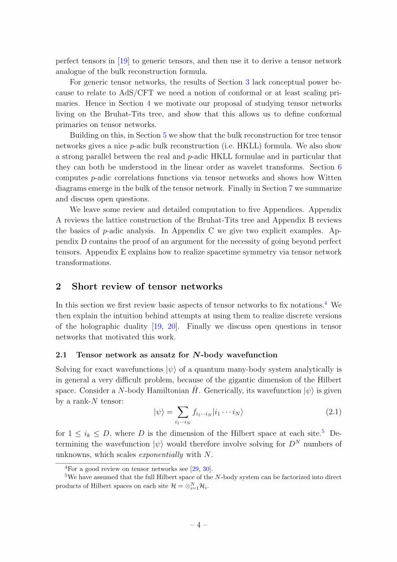
OI

OJ OK

w

Figure 5. “Non-linear” contributions to operator pushing. The bulk operator OI splits

into OJ and OK . They are subsequently propagated to 1 (blue) and 2 (red) respectively.

Namely, a operator acting OI in the bulk can be “reconstructed”, to linear order,

by a sum over the same operator acting on the boundary edges weighted by the

“smearing function” KI .

3.4 Non-linear orders in HKLL

Now we move on to the non-linear terms in the global operator pushing formula

(3.10). Using the same basis that diagonalizes the linear order global operator push-

ing in (3.12), we now compute the coefficient AIJK(v, i|j, k), which corresponds to

pushing the operator OI all the way to the two boundary operators OJ acting on

the boundary leg j and OK on the boundary leg k.

Now we use the same argument as the one for the linear term of the global

pushing. Since there are two operators at the boundary links j, k, the contribution

to AIJK(v, i|j, k) involves splitting the operator OI into OJ and OK , at some bulk

vertex w. A contribution comes from a product of local operator-pushing coefficient

αII along the path P that joins the initial vertex v to the mid-way bulk vertex w.

At w we use the local operator pushing coefficient αIJK obtained in (3.9) to split

the operator OI into OJ and OK . Then we push these operators OJ and OK along

paths P(w → j) and P(w → k), respectively. Finally, we sum over all paths and the

mid-way bulk vertex w. (See Figure 5.)

The final result is

AIJK(v, i|j, k) =∑w

GI(v|w)αIJK KJ(w | j)KK(w | k), (3.16)

– 15 –

where we have defined the bulk-bulk kernel

GI(v|w) ≡∑Pλ|P(v→w)|I (3.17)

where the sum is over all paths that connect two bulk vertices v and w. Note that

the bulk-bulk kernel GI(v|w) and the “smearing function” KI(v|j) are simply related

by taking the w all the way to the boundary leg j.17 This can be compared with the

bulk-bulk reconstruction kernel in [36] that we quoted in (3.1).

Higher order coefficients AIJKL···(v, i|j, k, ` · · · ) can be obtained in the same way.

For example,

AIJKL(v, i|j, k, `) =∑w

GI(v|w)αIJKLKJ(w|j)KK(w|k)KL(w|`)

+∑w,u

(GI(v|w)αIJM KJ(w|j)GM(w|u)αMKLKK(u|k)KL(u|`)

+GI(v|w)αIKM KK(w|k)GM(w|u)αMJLKJ(u|j)KL(u|`)

+GI(v|w)αIMLKL(w|`)GM(w|u)αMJK KJ(u|j)KK(u|k)

).

(3.18)

For a tensor network defined on a tree, this is the complete set of contributions.

In a generic network with loops, these contributions will be dressed by loop diagrams.

A complete analysis of these loop diagrams is beyond the scope of the current paper.

In the following, we will focus on tree networks.

4 Tensor networks on p-adic tree

In this section we motivate the study of tensor networks living on the p-adic tree

as an explicit example of discrete AdS/CFT. We emphasize its difference from ten-

sor networks based on regular tessellations of AdS. It can be viewed as an explicit

realization of p-adic AdS/CFT recently proposed in [26, 27].18

4.1 From tessellation to tree

4.1.1 Limitation of tensor networks based on regular tessellation

In the AdS/CFT correspondence, the global symmetries of the boundary CFT are

mapped to isometries of the bulk spacetime. When using tensor networks to model

17For infinite networks, we need to regularize this limit.18Note that the relation of p-adic AdS/CFT to the tensor network was also mentioned in [26],

although it was based on geometric embedding of the p-adic tree in regular tessellation of AdS, as

opposed to an abstract tree.

– 16 –

holography, the network G corresponds to the bulk space. To realize a discrete version

of AdS, the most common approach is to choose G based on a regular tessellation. The

bulk isometry is then the discrete subgroup of SL(2,R) preserved by the particular

tessellation.

For example, when the basis tile is a hyperbolic triangle with

Triangle (π

`,π

m,π

n) with

1

`+

1

m+

1

n< 1 (4.1)

the isometry group of G is the triangle group W [`,m, n]. For generic types of tilings

(made of basic triangles), the isometry group is a reflection group19 (or more ab-

stractly Coxeter group), i.e. generated by reflections across the edges of the tiles.

Figure 6(a) shows the hexagon tensor network based on the W[2, 4, 6] tilling. A brief

review and relevant references can be found in [21].

(a) (b) (c)

Figure 6. Tensor network embedded in a regular tessellation of Poincare disk. (a):

Hexagon tensor network, based on W[2, 4, 6] tilling. (b): A 4-valent tree tensor network,

based on the spanning tree of W[2, 4, 6] tilling. (c): 3-valent tree tensor network, based on

W[∞, 2, 3] tiling.

However, the representation theory of Coxeter groups is not strong enough to

help find the bulk solutions (living on the graph G). As a contrast, in the usual

AdS/CFT, the bulk solution can be solved explicitly in terms of irreducible repre-

sentations of the conformal group. In particular, one can find the bulk solutions that

are dual to primary operators of the boundary CFT. For tensor networks, to proceed

to more quantitive comparisons between the bulk and the boundary, we need a better

handle on the isometry group of the graph G.20

19Note that rotations can be generated by successive reflections across different edges. For text-

books on hyperbolic reflection groups see e.g. [37].20We are not aware of a systematic discussion of graph wavefunctions defined on regular tilings

of the hyperbolic space, or if such solutions exist at all, how they organize themselves into repre-

sentations of the Coxeter group.

– 17 –

4.1.2 Tensor networks on abstract tree

The isometry of the tensor network based on a regular tiling is a discrete subgroup

of SL(2,R) because we insist on the tensor network to be geometrically embedded

in AdS2, respecting its isometry. However, there is no a priori reason that the

discretization should work in this most naive form. Suppose we relax this assumption,

i.e. we view the lattice as an abstract lattice, free from the underlying AdS, then it

is possible for the lattice to furnish a different, possibly bigger, symmetry.

In this paper, we adopt the somewhat radical approach of giving up the geometric

embedding in order to gain more symmetry. Since modeling AdS/CFT is our main

goal, we still want this symmetry to be related to the conformal symmetry in some

way. It turns out that the (p+1)-valent tree with p being a prime number can furnish

a representation for the full conformal group of SL(2,Qp) where Qp is the field of

p-adic numbers. This is a continuous group and hence much bigger than a discrete

subgroup of SL(2,R).

This consideration is inspired by the recently discussed p-adic AdS/CFT cor-

respondence [26, 27]. The proposed duality is a discrete analogue of AdS/CFT. In

the simplest example where the bulk is two dimensional and the boundary one di-

mensional, the bulk geometry is given by the Bruhat-Tits (BT) tree, whereas the

boundary is conjectured to be a theory that is defined on the field Qp i.e. the p-adic

numbers, and which preserves the SL(2,Qp) symmetry.

Before moving on to a review of the p-adic tree, we emphasize that, different

from [26], we do not view it as arising from a regular tessellation of the real AdS.

There are two ways a tree can arise from tessellations. The first is the spanning tree

of the graph of a tessellation — we draw the spanning tree of the tessellation based

on W[2, 4, 6] in Figure 6(b).21 The second is when the triangle group is W[∞, 2,m],

which results in a m-valent tree. Figure 6(c) shows an example of the 3-valent tree.

However, the trees that arise from these two ways completely break the scaling

symmetry of the underlying AdS space.22 In contrast, the p-adic tree we will be

considering furnishes the full SL(2,Qp) symmetry.

4.2 p-adic number field and Bruhat-Tits tree

In this section we review the p-number field Qp and its Bruhat-Tits tree, to prepare

for the discussion of the Bruhat-Tits tree and p-adic AdS/CFT, and to fix notation.

For textbooks on p-adic numbers, see [38, 39]. For its applications in string theory

or other fields of mathematical physics, we recommend [40–46].

21Given a lattice, its spanning tree is a tree that contains all the vertices of the lattice and has

the minimal number of edges.22For a regular tessellation based on the triangle group W[`,m, n] in which all three numbers are

finite, there are some discrete scaling symmetries preserved by the tessellation. However, this is not

enough for any quantitive calculation we want to do in this paper.

– 18 –

4.2.1 The field Qp of p-adic numbers

The field of rational numbers Q can be extended to the field of real numbers R, with

respect to the Euclidean norm |x|, which satisfies a few axioms.

(1) : |x| ≥ 0 (2) : |x| = 0↔ x = 0 (3) : |x y| = |x| |y| ∀x, y ∈ R(4) : |x+ y| ≤ |x|+ |y| ∀x, y ∈ R (triangle inequality)

(4.2)

Starting with the rational field Q, it is possible to extend it in other ways, with

respect to different norms that obey the above axioms.

Given a prime number p, a rational number x ∈ Q can be uniquely expanded in

terms of powers of p:

xp =∞∑

n=−Nan p

n with an ∈ Fp (4.3)

where Fp denotes the residue field consisting of integers 0, 1, . . . , p−1. The expansion

(4.3) can be rewritten to highlight the congruence of xp with respect to p, i.e. the

leading term of the p-adic expansion:

x = pvp(x)

∞∑n=0

bn pn with b0 6= 0 , bn ∈ Fp and vp(x) ∈ Z (4.4)

using which the p-adic norm |x|p of x is defined as

|x|p ≡ p−vp(x) with vp(x) ∈ Z. (4.5)

Namely, the more divisible x is w.r.t. p, the smaller norm it has.

It is then easy to check that the p-adic norm obeys all four axioms for the norm.

In fact, it satisfies an even stronger form of the fourth axiom:23

|x+ y|p ≤ max(|x|p, |y|p) (strong triangle inequality) (4.6)

We thus see that the rational field Q can have infinitely many different norms:

the Euclidean norm |x| together with the p-adic norms |x|p for each prime p.24 The

real field R is only one possible extension of Q, using the Euclidean norm |x|. Now,

for each prime p, we can have a different extension of Q using the p-adic norms |x|p.Given a fixed prime number p, the field Qp consists of all possible formal expansions

of the form:

Qp ≡ {xp =∞∑

n=−Nan p

n | an ∈ Fp}. (4.7)

23Note that the original triangle inequality is trivially satisfied by the p-adic norm: |x + y|p ≤|x|p + |y|p.

24The Euclidean norm |x| and the p-adic norm |x|p are the only possible norms to complete the

rational field Q (giving R and Qp, respectively), as already shown by Ostrowski in 1919 [47].

– 19 –

The p-adic norm (4.5), in particular |pn|p = 1pn

, ensures that the formal series (4.7)

converges.25 The strong triangle inequality (4.6) also implies |x + x|p ≤ |x|p, which

violates the Archimedes principle |x+x| ≥ |x|— hence the geometry based on p-adic

norm is called non-Archimedean.

The p-adic norm is used to define the following subset of Qp, which will be

useful in the later construction of the Bruhat-Tits tree and the discussion on p-adic

integration. First, the unit sphere in Qp consists of xp with unit norm:

Up ≡ {xp ∈ Qp | |x|p = 1} i.e. x|p = a0 + a1p+ a2p2 + . . . a0 6= 0 (4.8)

The unit ball of Qp is inside Up:

Zp ≡ {xp ∈ Qp| |x|p ≤ 1} i.e. x|p = a0 + a1p+ a2p2 + a3p

3 . . . (4.9)

Note that the unit ball Zp is precisely the ring of p-adic integers. However, unlike Z(which is open in R), Zp is both open and closed (“clopen”) in Qp. Finally, we denote

the set of non-zero elements in Qp as Q∗p ≡ Qp/{0}, which is Q∗p ≡∐

n∈Z pnUp.

4.2.2 Bruhat-Tits tree as bulk of p-adic line Qp

In this subsection we summarize the construction of the Bruhat-Tits tree [48, 49], in

particular motivating it from its role as the bulk of Qp (i.e. the analogue of upper

half plane but whose boundary is Qp instead of R) and prepare for the discussion on

the SL(2,Qp) action on the tree.

The real field R is the boundary of the upper half plane H ≡ SL(2,R)/SO(2,R).

With coordinates H ≡ {z = x+ i y |x ∈ R, y ∈ R+}, it has SL(2,R)-invariant metric

ds2 = 1y2

(dx2 + dy2). An SL(2,R) action on a point z = x + i y on H would induce

the same action on its boundary point x. If we replace the boundary space R by the

p-adic field Qp, what would be its bulk, i.e. what is the p-adic version of the upper

half plane?

The analogy with the relation between H and its boundary R, shown in Table 1

suggests that one should replace R by Qp in the definition of H to give

Hp ≡PGL(2,Qp)

PGL(2,Zp). (4.10)

We immediately see the difference from the real case. As the maximal compact

subgroup of the isometry group PGL(2,Qp), PGL(2,Zp) is both open and closed

(“clopen”) in PGL(2,Qp). Therefore, although Qp is a continuum, its bulk Hp is

actually discrete.

25Note that in contrast to the decimal expansion for the real number x ∈ R, for a p-adic number

xp ∈ Qp, we allow the expansion to be infinite in the direction of the positive exponent of p but

not along the negative direction, precisely because a higher power of p has a smaller p-adic norm.

– 20 –

upper half plane H Bruhat-Tits tree Hp

Isometry group G SL(2,R) PGL(2,Qp)

Isotopy group K SO(2,R) PGL(2,Zp)Boundary R Qp

Table 1. The parallel between the upper half plane H and the Bruhat-Tits tree Hp.

Since Hp has a discrete topology, we cannot simply give Hp the coordinate zp =

xp + i yp in which xp ∈ Qp and yp ∈ Qp+ and write down the PGL(2,Qp) invariant

metric on it. However, the coset expression (4.10) suggests that one can construct it

as a set of equivalence classes 〈〈~f,~g〉〉 of lattices 〈~f,~g〉 in Qp⊗Qp, where two lattices

are equivalent, 〈~f,~g〉 ∼ 〈~f ′, ~g′〉, iff

(~f ′, ~g′) = (Γ · ~f,Γ · ~g) with Γ ∈ PGL(2,Zp). (4.11)

We leave the details of the construction to the appendix. To summarize, the p-adic

analogue of the upper half plane Hp has the topology of an infinite (p+1)-valence tree

(called Bruhat-Tits tree). The nodes on the tree are defined as equivalence classes

〈〈~f,~g〉〉 of lattices 〈~f,~g〉 and have the form

〈〈(pm

0

),

(x(m)

1

)〉〉 x(m) =

m−1∑n=−N

anpn an ∈ Fp. (4.12)

Note that since x(m) truncates at pm, we can think of pm as giving the accuracy level

of a p-adic number x(m), i.e. the node (4.12) represents the equivalence class

x(m) + pmZp. (4.13)

This somewhat formal definition of the Bruhat-Tits tree as equivalence classes of

lattices in Qp⊗Qp actually connects nicely with the p-adic expansion of the bound-

ary Qp. First note that the p-adic expansion already has a natural tree structure.

Consider a generic p-adic number

. . . a3 a2 a1 a0 . a−1 a−2 a−3 . . . a−N (4.14)

First, start from level p0, there are p choices for the coefficient a0, draw a node for

each choice. The node with a0 = 0 is then the origin O. Starting from each node

(labeled by a0) at level p0, there are again p choices for a1 — draw these p nodes at

level p1 and connect them to the node they start from. Moving up this way (and

also connecting all nodes at p0 backwards to the node the correspond to 0p−1 + 0),

one draws an infinite (p + 1)-valent tree starting from level p−1. Moving backwards

towards negative powers p−n then gives the entire Bruhat-Tits tree.

– 21 –

Thus we obtain a one-to-one map between a p-adic number and a branch on the

Bruhat-Tits tree: given a p-adic number, its branch is defined by starting from the

lowest power of the expansion (4.14) and then at each level pn following the twig

corresponding to an in the expansion (4.14). Each node in the bulk Bruhat-Tits tree

has two label:

z = x(m) z0 = pm (4.15)

where pm gives the accuracy level and x(m) a p-adic number to the accuracy pm, i.e.

it represents the equivalence class x(m) + pmZp. This precisely agrees with the result

from the lattice construction of the Bruhat-Tits tree.

The non-zero elements in Qp can be grouped according to the leading term in

the p-adic expansion:

Q∗p =∐n∈Z

pnUp : x|p = pv u with v ∈ Z and u ∈ Up (4.16)

i.e. u =∑∞

n=0 an pn with a0 6= 0. The set pnUp for each n ∈ Z forms a subtree with

the root at:

Points on the main branch: x(n)0 = pn · 0 with accuracy pn (4.17)

The line connecting all the x(n)0 is then the main branch, running from n→ −∞ to

n→ +∞.

4.3 Conformal primaries for tensor network on Bruhat-Tits tree

Recall that the main disadvantage of viewing the network G as a naive discretization

of the substrate AdS space is that it retains too few symmetries and makes it diffi-

cult to organize operators. We now show that identifying the tree network G as the

Bruhat-Tits tree preserves a full conformal SL(2,Qp) symmetry26 for the tensor net-

work, and in particular allows us to define conformal primaries for operators acting

on the tensor network.

4.3.1 SL(2,Qp) action on Bruhat-Tits tree

The coordinate system (4.12) assigns a vertex on the Bruhat-Tits tree two numbers

pm and x(m). In order to determine the radial direction and the boundary direction,

and how to choose the cutoff surface in a manner suitable to holography (and anal-

ogous to the upper half plane in the real case), we now study their behavior under

the bulk PGL(2,Qp) action.

A PGL(2,Qp) transformation acts on the lattice via

〈~f,~g〉 → 〈γ · ~f, γ · ~g〉 with γ =

(a b

c d

)∈ PGL(2,Qp). (4.18)

26Here we are a bit cavalier in our notation: the actual group that acts is PGL(2,Qp), but we

shall often (in analogy with the table above) refer to it as SL(2,Qp).

– 22 –

Given a vertex on the Bruhat-Tits tree with coordinate (4.12), under a PGL(2,Qp)

action, it transforms as

〈〈(pm

0

),

(x(m)

1

)〉〉 −→ 〈〈

(pm′

0

),

(a x(m)+bc x(m)+d

1

)〉〉 (4.19)

where

pm′= pm

∣∣∣∣(c x+ d)2

ad− bc

∣∣∣∣p

. (4.20)

Namely, start with the bulk point x =∑m−1

n=−N an pn , with accuracy only up to level

pm, its SL(2,Qp) image is another bulk point at

a x(m) + b

c x(m) + d=

m′−1∑n=−N

bn pn with accuracy pm

′. (4.21)

It is quite remarkable that the Bruhat-Tits tree, though discrete, can furnish the

full conformal group PGL(2,Qp). This allows us to study the function on the tree

which has a definite quantum number. Given the Iwasawa decomposition G = NAK,

where N is the Borel subgroup, A the dilation, and K maximal compact subgroup

SL(2,Zp), it is enough to look at their actions separately. The most important is the

scaling transformation. Under a dilatation by pn, a vertex on the tree transforms as

D =

(pn/2 0

0 p−n/2

): 〈〈

(pm

0

),

(x(m)

1

)〉〉 −→ 〈〈

(pm+n

0

),

(pnx(m)

1

)〉〉. (4.22)

The action moves the branches along the main branch, shown in Figure 7.

4.3.2 Choice of cutoff surface

The construction of a holographic correspondence includes a prescription on how the

boundary is approached from inside the bulk, i.e. how to define the cut-off surface

which is then pushed to infinity. For instance, AdS in global coordinates or Poincare

coordinates have different natural cut-off surfaces and therefore different boundary

behaviors. Now we show that the cut-off surface natural to the Bruhat-Tits tree

should be lines of constant pm.

As we go to the boundary, both m and m′ →∞,

x(m) =m−1∑n=−N

an pn −→ x =

∞∑n=−N

an pn (4.23)

we have the expected boundary PGL(2,Qp) transformation:

x =∞∑

n=−Nan p

n −→ a x+ b

c x+ d=

∞∑n=−N ′

bn pn (4.24)

– 23 –

0

x ∈ Qp

p2

p1

p0p0

p−1

pm

p

p2

1

110110

.1

1.10.1

Figure 7. Bruhat-Tits tree for p = 2. The dilatation D on the tree slides the branches

along the main branch.

Let’s compare to the real case. Under an SL(2,R) on a point z = x+ i y in the

upper half plane H, x and y transform as

x −→ (a x+ b)(c x+ d) + a c y2

(c x+ d)2 + (c y)2

y→0−−→ a x+ b

c x+ d

y −→ y

(c x+ d)2 + (c y)2

y→0−−→ y

(c x+ d)2

(4.25)

Comparing this with the transformation of x(m) in (4.24) and pm in (4.20), we con-

clude that pm should play the role of the holographic direction, the analogue of y

in the real case, whereas x(m) the role of the boundary direction. This also means

that the cut-off surface should be a line of constant pm, as shown in Figure 8. This

is analogous to the choice of the z = ε surface as the cut-off surface, where z is the

radial direction in Poincare coordinates.

4.3.3 Conformal primaries for p-adic tensor network

A primary field OI(x) of PSL(2,Qp) with conformal weight ∆I is defined as [50]

OI(a x+ b

c x+ d) =

(∣∣∣∣ det γ

(c x+ d)2

∣∣∣∣p

)−∆I

OI(x) where γ =

(a b

c d

)∈ PGL(2,Qp)

(4.26)

In particular, for a scaling transformation x→ p x

OI(px) = p∆IOI(x) (4.27)

– 24 –

p2

p1

p0p0

p−1

z0

p

p2

1 2 3 4 5 6 7 8

2

2

O O4

4

Figure 8. A tree tensor network together with its conjugate, glued together (in compu-

tation of correlators) along the common boundary, which is the analogue of the Poincare

cutoff surface in the BT tree. Tensors move down the tree under a scaling transformation.

We indicate with green arrows a few examples of how the links move. Such a transfor-

mation corresponds to a transformation of operators such that it is sandwiched between a

network tensor. This is depicted in the box.

Let’s translate this condition on operators in the tensor network.

Consider an operator OI acting on a boundary leg of the tensor network. One

important feature of the constant pm cutoff surface is that the external legs are not

evenly distributed, see Figure 8. The distance of the external legs from the main-

branch increases as we move along the cutoff surface. Therefore, under the scaling

transformation x→ pn x with n > 0, an operator acting on a given boundary leg on

the cutoff surface would hop from a branch closer to the main branch to branches

further away from the main branch.

For instance, under the boundary scaling x→ p x, an operator OI acting on leg

2 is mapped to OI acting on leg 4, and leg 4 to leg 8, and so on. Applying (4.26) to

this particular network, we have

OI(i2) = p−∆IOI(i4) (4.28)

As we will see later in Section 6, the condition such as (4.28), together with the

assumption on the homogeneity of the network, allows us to explicitly construct a

– 25 –

primary basis starting from the Pauli basis defined in (3.6), and moreover relate it

to the “operator pushing” basis defined in (3.13).

5 p-adic HKLL from tree tensor networks

In section 3 we derived the bulk operator reconstruction formula for generic tensors

using “operator pushing”. In this section we show that for tree tensor networks, it

matches nicely with the expectation from the conjectured p-adic AdS/CFT corre-

spondence.

5.1 HKLL for tree tensor network

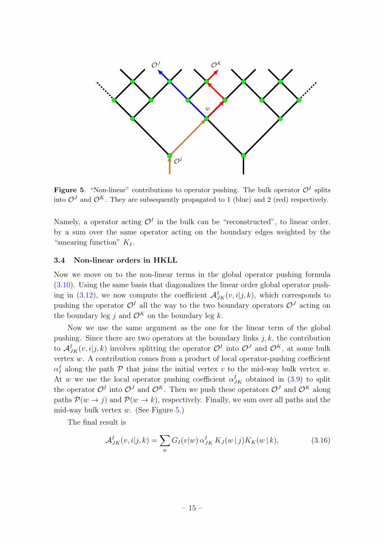
When the network G is an r = p+ 1 valent tree, the path from a bulk edge (say the

first edge of vertex v) to the boundary edge is unique. Therefore the linear term of

the global operator pushing (3.15) becomes

OI(v, 1) |Ψbulk〉 =∑i

(λI)|P(v→i)|OI(i) |ψbndy〉 (5.1)

where P(v → i) labels the unique path from the bulk vertex v to the boundary edge

i, and |P| measures its length. This is illustrated in Figure 9.

∂

OI(v)

OI(i)

KI(v, 1|i)

Figure 9. Linear contribution of global operator pushing for a tree tensor network.

It is exactly in the form of the HKLL formula

OI(v, 1) |Ψbulk〉 =∑i

KA(v, 1|i)OI(i) |ψbndy〉 (5.2)

with the “smearing function”

KI(v, 1|i) ≡ (λI)|P(v→i)| = p−σI |P(v→i)| (5.3)

where in the last step we have used the following definition

p ≡ r − 1 and σI ≡ −lnλIln p

(5.4)

– 26 –

Similarly, for the next order in the HKLL formula (3.16), the bulk-bulk kernel

defined in (3.17) is also greatly simplified for a tree tensor network:

GI(v|w) ≡ (λI)|P(v→w)| = p−σI |P(v→w)| (5.5)

Note that (3.16) is a sum of bifurcated paths from vertex v to the two boundary legs

j and k, with the sum over the bifurcating point w, as illustrated in Figure 10.

∂

OI(v)

OJ(j)OK(k)

w

AIJK

Figure 10. Non-linear contribution of global operator pushing for a tree tensor network.

In both the “smearing function” (5.3) and the bulk-bulk kernel (5.5) for an

operator OI , only one parameter σI (5.4) appears. What is its physical meaning?

To answer this, one first checks that both the “smearing function” (5.3) and the

bulk-bulk kernel (5.5) satisfy the expected EOM for a tree Lagrangian of a scalar

[51]:

(�v +m2I)GI(v|w) = NIδ(v, w) (�v +m2

I)KI(v|i) = 0 (5.6)

where the graph Laplacian � can be defined for a generic graph as27

�φ(v) =∑

v′∈nn(v)

(−φ(v′) + φ(v)) (5.7)

The sum is over all nearest neighbours of v. We see that the parameter σI is related

to the mass squared of the bulk scalar by

m2I = p1−σI + pσI − (p+ 1). (5.8)

For a finite network G, the “smearing function” can be simply obtained by taking

the second bulk vertex in the bulk-bulk kernel all the way to the boundary:

KI(v, 1|i) = limw→iGI(v|w). (5.9)

27Note the opposite sign from the usual definition — this is to match the mostly-negative signa-

ture.

– 27 –

For an infinite network, a regularization is needed to make KI(v, 1|i) finite.

One can now use the “smearing function” KI and the bulk-bulk kernel GI to

explicitly compute the tensor network analogue of the bulk operator reconstruction.

In the following, we move on to interpret these results in the light of p-adic AdS/CFT.

5.2 p-adic HKLL

The “smearing function” KI (5.3) and the bulk-bulk kernel GI (5.5) were derived us-

ing only “operator pushing” of the tensor network. Now we show that they have clear

meanings if the tree tensor network is interpreted as the bulk of p-adic AdS/CFT,

supporting our proposal that tree tensor network provides a concrete realization of

p-adic AdS/CFT.

5.2.1 Reconstruction kernel v.s. propagator

In p-adic AdS/CFT, the bulk propagator gI and the bulk-to-boundary propagator

kI of an operator with conformal dimension ∆I are [27]:28

gI(v|w) =ζp(2∆I)

p∆Ip−∆I |P(v→w)| and kI(v|i) =

ζp(2∆I)

ζp(2∆I − 1)p−∆I |P(v→i)|

(5.10)

where the conformal dimension ∆I is related to the mass of the scalar living on the

bulk Bruhat-Tits tree by

m2I = − 1

ζp(∆I − 1)ζp(−∆I)(5.11)

with the p-adic zeta function ζ(s) ≡ 11−p−s .

Comparing our result of the “smearing function” KI (5.3) and the bulk-bulk

kernel GI (5.5), derived here using the “operator pushing” for a tree tensor network,

with the boundary-to-bulk propagator kI and the bulk propagator gI of the p-adic

AdS/CFT derived in [27], we see that29

KI = kI |∆I→σI and GI = gI |∆I→σI . (5.12)

Given that the two pairs satisfy the same EOM, we should match the two expres-

sions for the bulk mass (5.8) and (5.11) and obtain a relation between the parameter

σI in (5.3) and the conformal dimension ∆I of the operator OI . A priori, there are

two solutions σI = ∆I or σI = 1−∆I .

Recall that in the real case, the “smearing function” (3.2) used for the bulk oper-

ator reconstruction is related to the bulk-to-boundary propagator by first replacing

28In this subsection we will mostly focus on the case with boundary dimension d = 1.29The normalizations of our smearing function and the bulk-bulk kernel will be fixed later using

two-point correlation functions and will turn out to be consistent with this identification.

– 28 –

the conformal dimension ∆I in the exponent by d − ∆I .30 Therefore, the natural

conclusion is

σI = 1−∆I . (5.13)

The relation (5.13) is valid for boundary dimension d = 1. In generic dimensions, it

should be replaced by

σI = d−∆I . (5.14)

We will prove this relation later in Section 6.

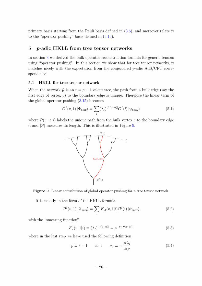
5.2.2 Reconstruction kernel in terms of p-adic variables

The relation (5.12) (together with (5.13)) between the reconstruction kernels for tree

tensor networks and the propagators of p-adic AdS/CFT shows that the reconstruc-

tion kernels (5.3) and (5.5) we derived using the “operator pushing” are consistent

with the expectation of the conjectured p-adic AdS/CFT. We now compare these

reconstruction kernels to the HKLL formula for the real AdS/CFT and show that

the tensor network provides a nice p-adic HKLL formula.

To compare with the real HKLL, we first need to rewrite the “smearing function”

KI(v|i) (5.3) in terms of p-adic variables. Interpreting the tree on which the tensor

network lives as the Bruhat-Tits tree, we should assign the bulk point v coordinates

that label a node on the Bruhat-Tits tree as in (4.15). Namely, we start from a point

on the boundary x ∈ Qp, and follow the (unique) path connecting it to the origin of

the tree, and label the bulk point v on the level m as (x, z = pm). For the boundary

edge i in KI(v|i), we simply assign a p-adic number y:

bulk vertex v : (x ∈ Qp, z = pm) and boundary edge i : y ∈ Qp (5.15)

with m ∈ Z denotes the holographic direction in the BT tree, and gives the accuracy

of the p-adic expansion. In particular, |z|p = p−m, and |z|p → 0 as one approaches

the boundary.

It was shown in [27] that the distance from a bulk vertex on the Bruhat-Tits

tree to a boundary point, in the coordinates above, is

|P(v → i)| = −logp|z|p

sup{|z|p, |x− y|p}2(5.16)

where the supremum norm is sup{|z|p, |x− y|q} = |z|p if |z|p ≥ |x− y|p and |x− y|potherwise. Using (5.16) we have31

KI(x, z | y) =ζp(2∆)

ζp(2∆− 1)

( |z|psup{|z|p, |x− y|p}2

)d−∆I

(5.17)

30The Θ function appearing in [52] is introduced as a regularization via analytic continuation of

the bulk integral.31We emphasize that the HKLL relation here is not to be confused with the bulk reconstruction

discussed in [26], which is the Euclidean version of recovering the bulk field for specified Dirichlet

boundary condition, which use the non-normalizable bulk-to-boundary propagator as in (5.10).

– 29 –

Finally, recall that in the real HKLL formula one needs to regularize the bulk

integration to have finite results. In Poincare coordinates, this is done by dressing

the “smearing function” with a Θ((~x− ~y)2− z2) factor. In an actual tensor network

computation, the tree is usually taken to be finite. However, the tensor network

modeling p-adic AdS/CFT needs to live on the infinite Bruhat-Tits tree. Therefore

we propose to regularize by dressing the p-adic smearing function (5.17) with the

p-adic analogue of the Θ function — a factor of γ(x−yz

) where γ is the characteristic

function of Zp in Qp defined in equation (B.7):

KI(x, z | y) =ζp(2∆)

ζp(2∆− 1)

( |z|psup{|z|p, |x− y|p}2

)1−∆I

γ(x− yz

). (5.18)

We see the p-adic HKLL formula, derived using the tensor network, uses a p-adic

smearing function (5.18) that is completely parallel to the smearing function (3.2)

for the real HKLL formula. Next we show that the linear term of the bulk operator

reconstruction

φp(x, z) =

∫Qpdy Kp(x, z |y )O(y) (5.19)

can be interpreted as a p-adic wavelet transform.

5.3 Linear term of HKLL as wavelet transform

In this subsection we show that the linear term of the bulk reconstruction can be

interpreted as a wavelet transform — a technique in signal processing, analogous to

the Fourier transform but with Fourier modes replaced by the wavelet basis.

As will be reviewed later, the wavelet transform has a built-in coarse graining

process, therefore can be regarded as a realization of RG flow. For a comprehensive

review of the subject, see [53]. This underlies the connection between wavelet trans-

forms and AdS/CFT. In the context of tensor networks, it is recently found to be

implementable in MERA [54]. In [24] (see also [25]) the Haar wavelet was used to

construct a holographic mapping in a particular example of tensor network.

We will show that the (linear term) of the bulk reconstruction is exactly a wavelet

transform, with the choice of wavelet determined universally, by AdS/CFT. We fur-

ther show that the inverse of the bulk reconstruction is actually not the inverse

wavelet transform, but needs to be regularized. We propose a regularization natural

to the HKLL formula. Both the real and the p-adic case work in this manner.

5.3.1 Wavelet review

We now review basics of wavelet transforms, using the notations in [55], whose dis-

cussion makes the parallels with the HKLL relation particularly transparent.

The wavelet basis containing d+1 parameters is defined as follows. First, choose

the mother wavelet ψ(~x), which is a (local) function of d parameters ~x. The set

– 30 –

of daughter wavelets is generated from the mother wavelet by translation by ~a and

rescaling by s:

ψ~a,s(~x) ≡ 1

sd/2ψ(~x− ~as

), (5.20)

These daughter wavelets form the wavelet basis.

Given a signal function f(~x), the wavelet transform using the wavelet ψ is then

defined as32

Wf (~a, s) =

∫ddx f(~x)ψ†~a,s(~x) , (5.21)

For a generic mother wavelet ψ(~x), the wavelet basis {ψ~a,s(~x)} it gives rise to is

over-complete. However, special types of mother wavelet ψ(~x) can allow an inverse

transform. Relevant to the case at hand is when

ψ(~k) = ψ(k) , (5.22)

where ψ(~k) is the Fourier transform of ψ(~x) and k ≡ |k|. One can show that then

the inverse transform of (5.21) exists and is given by

f(~x) =1

Cψ

∫ ∞0

ds

sd+1

∫ddaWf (~a, s)ψ~a,s(~x) (5.23)

where

Cψ ≡∫ ∞

0

dk|ψ(k)|2k

(5.24)

Note that for the inverse transform to be well-defined, we also need the following

“admissibility condition”

Cψ < +∞ (5.25)

It is often more convenient to apply the wavelet transform in Fourier space.

Consider Fourier transforming (5.21) w.r.t. ~a. This gives

Wf (~k, s) = g(~k, s)f(~k) with g(~k, s) ≡ 1

sˆ(ψ†)s(−~k) (5.26)

It means that to define the mother wavelet of a wavelet transform, we could equiva-

lently specify a function g(~k, s) which is a function of the momentum and the scale

factor s.

5.3.2 Real linear HKLL as real wavelet

The linear term of the bulk reconstruction (3.1) is very close to a wavelet transform

with the mother wavelet

ψ∆(~x) =

(1

1− ~x2

)d−∆

Θ(1− ~x2) (5.27)

32Using the analogy with the Fourier transform, if ~x is regarded as the spacetime variable, the

parameter ~a and s together play the role of momentum variables.

– 31 –

where Θ is the step function with Θ(x) = 1 for x ≥ 0 and Θ(x) = 0 for x < 0. Her

daughter wavelets, defined via (5.20), and the HKLL “smearing function” are related

by a scaling

K(~x, z | ~y ) = z∆− d2ψ~x,z(~y) (5.28)

We interpret this result as follows. The AdS/CFT correspondence selects for us

a set of wavelet transform: for each operator O∆ of conformal dimension ∆, there is

a mother wavelet ψ∆ such that the wavelet transform WO(~x, z), which is related to

the bulk fields φ(~x, z) via

φ(~x, z) = z∆− d2WO(~x, z) (5.29)

becomes a weakly-coupled and semi-classical degree of freedom. The holographic

direction “z” in Poincare coordinates is identified with the scaling parameter of the

wavelet transform.

Now let’s look at the inverse transform. For the standard inverse wavelet trans-

form (5.23) to exist, the admissibility condition (5.25) needs to be satisfied. For a

scalar field, the conformal dimension is ∆ = d/2 + ν with ν =√d2/4 +m2. The

Fourier transform of (5.27) is

ψ∆(k) =Jν(k)

kν(5.30)

which gives

Cψ =

∫ ∞0

dkJν(k)2

k2ν+1∼ Γ(0)→∞ (5.31)

i.e. Cψ diverges and the inverse wavelet transform (5.23) is no longer valid. However,

this does not pose a problem for us because, although we use the wavelet trans-

form to obtain the bulk field, we actually do not need to use the (standard) inverse

wavelet transform (5.23) to obtain the boundary operator from the bulk field. We

can compute instead ∫ddx dz

√gAdSd+1

φ(~x, z)K(~x, z|~y) , (5.32)

which has an extra dressing factor of z2ν relative to the integration measure of the

(standard) inverse wavelet transform (5.23). (The scaling parameter “s” there is to

be identified with “z” in the Poincare coordinate here.) This is a natural choice in

AdS geometry.

The Fourier transform of the smearing function is [34]

K(~x, z | ~y) = N∫

time-like

ddk

(2π)dzd/2Jν(kz)

kνei~k·(~x−~y) (5.33)

where k =√−~k2 and N the normalization constant. The integral is restricted to

time-like momenta so that Jν remains normalizable. Plugging (5.33) into (5.32), and

– 32 –

using

Cν ≡∫ ∞

0

dz

zJν(kz)

2 =1

2ν(5.34)

for time-like momenta k, we are left with

N 2

2ν

∫time-like

ddk

(2π)dk−2ν O∂(x′) ei~k·~y. (5.35)

Note that the integral (5.34) is the normalization that replaces Cψ in the wavelet

transform (5.23). The normalization condition Cν < +∞ in the inverse transform

(5.32) replaces the “admissibility condition” (5.25) that appears in the wavelet trans-

form (5.23). The restriction to time-like momenta is due to this normalization con-

dition, without which the integral is not finite. The restriction however means that

the reconstruction of the original operator O∂ is restricted by causality. Namely,

equation (5.35) can be re-written as

N 2

2ν

∫ddx′O∂(~x′)G(~x′ − ~y), (5.36)

where

G(~x′ − ~y) =

∫time-like

ddk

(2π)dk−2νeik·(~y−~x

′). (5.37)

This should be contrasted with the usual wavelet transform where the admissibility

condition is usually satisfied for all k.

5.3.3 p-adic linear HKLL as p-adic wavelet

Just as in the real case, the linear term of the p-adic bulk operator reconstruction can

be regarded as the p-adic wavelet transform of the boundary operator. The wavelet

transform perspective of the HKLL relation can be defined in an analogous manner

in the p-adic version of AdS/CFT. Let’s focus on the one-dimensional case.

p-adic wavelet transform. Given a p-adic mother wavelet ψ(x), which for our

purpose is taken to be a complex function with p-adic argument x, her p-adic daughter

wavelets can be defined in analogue to the continuous case (5.20)

ψa,s(x) =1√|s|p

ψ(x− as

) x, a, s ∈ Qp (5.38)

This set of daughter wavelets forms the basis for the p-adic wavelet transform. Then

the p-adic wavelet transform of a function f(x) with x ∈ Qp using this wavelet basis

is

Wf (a, s) =

∫Qpdx

1√|s|p

ψ†(x− as

)f(x) (5.39)

whose inverse transform is given by

f(x) =1

Cψ

∫Q×p

ds

|s|2p

∫QpdaWf (a, s)ψa,s(x) (5.40)

– 33 –

with

Cψ ≡∫Qpdk|ψ(k)|2pk

(5.41)

Note that the integration measure dsda|s|2p is precisely the left-invariant measure of the

p-adic affine group (whose action is x→ sx+ a). For the inverse transform to exist,

we need the same “admissibility condition” Cψ < +∞, as in the real case.

Just as in the real case, we can interpret the linear term of the bulk operator

reconstruction

φp(x, z) =

∫Qpdy Kp(x, z |y )O(y) (5.42)

as a p-adic wavelet transform (5.39). We first simplify the “smearing function” (5.18)

into

KI(x, z | y) = Np |z|∆I−1p γ(

x− yz

) with Np ≡ζp(2∆)

ζp(2∆− 1)(5.43)

Now we see a major difference from the real case. For the p-adic case, the choice of

the mother wavelet does not depend on the conformal dimension ∆ of the boundary

operator. For any operator, there is a “universal” mother wavelet

ψ(x) = Np γ(x) (5.44)

The conformal dimension ∆ only enters through the relation between her daughter

wavelets and the “smearing function”:

Kp(x, z | y ) = |z|∆−12

p ψ†x,z(y) (5.45)

which in turn gives the mapping between the wavelet transform WO(x, z) and the

bulk field:

φp(x, z) = |z|∆−12

p WO(x, z) (5.46)

Similar to the real case in (5.31), our mother wavelet (5.44) does not obey the

standard admissibility condition since

Cψ = N 2p

∫Qp

dk

|k|pγ(k)2 = N 2

p

∫Zp

dk

|k|p→ +∞ (5.47)

where we have used the fact that γ is self-dual under Fourier transform. Again, this

does not pose a problem for us, because the physical inverse transform we use to

obtain the boundary field O(y) is∫Q×p

dz

|z|2p

∫Qpdx φ(x, z|y)Kp(x, z|y) (5.48)

– 34 –

which has an extra dressing factor of |z|2∆−1, due to (5.45) and (5.46). We will now

show that this can make the normalization C finite and the inverse transform (5.48)

valid. Note that similar to the real case (5.27), the function γ restricts the integration

within the “causal patch” in the tree. (In the Bruhat-Tits tree, the causal future of

a node (x, z) is defined as the subbranch of the tree rooted at this node.33)

First we compute the Fourier transform of the p-adic “smearing” function (5.18),

using the additive character (B.5):

Kp(x, z | y ) = Np |z|∆p∫Qpdk e−2πi[k (x−y)] γ(kz) (5.49)

Note that since the function γ is self-dual under the Fourier transform, in the mo-

mentum domain the restriction to time-like momenta is also implemented by the γ

function. Plugging (5.49) into the inverse transform (5.48) we get

(N 2p Cp)

∫Qpdx′Gp(x

′ − y)O(x′) (5.50)

with

Gp(x′ − y) ≡

∫Qpdk |k|−2ν

p e−2πi[k(x′−y)] (5.51)

the p-adic analogue of the kernel in (5.37), and34

Cp =

∫Qpdz|z|2ν−1

p γ(z)2 =

∫Zpdz|z|2ν−1

p =p− 1

p(1− p−2ν)for ν > 0 (5.52)

with ν = ∆ − 12. Therefore, for all ν > 0, i.e. for massive scalars, the p-adic

normalization Cp is finite and the inverse transform is valid.

We have thus shown that the p-adic bulk reconstruction works in the same

manner as the real case: the bulk reconstruction can be realized as a continuous

wavelet transform, whereas the inverse, i.e. obtaining the boundary field from the

bulk one, is related to the standard inverse wavelet transform by an extra dressing

factor of z2ν .

There is one important difference between the real and the p-adic cases. In the

derivation of the bulk reconstruction via a p-adic wavelet transform, we have used

the continuous wavelet transform. However, in essence, the p-adic wavelet transform

is discrete.35 The reason is the following. First of all, even though we started with a

continuous wavelet transform in (5.39), the resulting scaling parameter is |z|p instead

33The causal structure on the Bruhat-Tits tree was first studied in [56], in the context of the

hierarchical structure of inflation.34Note that the integral in Cp only converges when ν > 0.35The coincidence of the continuous and the discrete p-adic wavelet transform was already shown

for a particular type of wavelets in [57].

– 35 –

of z. And since the integration measure in the inverse transform (5.40) is invariant

under the affine group, the integration is actually equivalent to the sum over the

Bruhat-Tits tree [27]: ∫Q×p

dz

|z|2p

∫Qpdx f(x, z) =

1

ζp(1)

∑v∈Tp

f(v) (5.53)

Recall that the Bruhat-Tits tree can be viewed as the discrete, holographic bulk

whose boundary is the continuous line of Qp. The emergence of the discrete p-adic

wavelet transform starting from a continuous one can be viewed as the mirror state-

ment of the above. This strongly supports the connection between the bulk recon-

struction and the wavelet transform, with the coordinate of the holographic direction

in the bulk being identified with the scaling parameter in the wavelet transform.

6 Correlation functions and emergent Witten diagrams

In this section we compute correlation functions of conformal primaries on a p-adic

tree tensor network, and show that dual Witten diagrams emerge automatically in

the bulk of the tensor network. We also explain the connection between the bulk

operator reconstruction in Section 5 and the correlation function computation.

6.1 Constructing conformal primaries in p-adic tensor network

An n-point correlation function in a tensor network is defined as

〈ψbndy|OI1(i1)OI2(i2) . . .OIn(in)|ψbndy〉 (6.1)

where the n boundary operators {OIi} are sandwiched between the original “bra”

wavefunction |ψbndy〉 defined in (2.8) using the tensors T and its conjugate “ket”

〈ψbndy|.36

To evaluate the n-point function (6.1) explicitly, we first need to construct con-

formal primaries {OIi}. The conformal primary for a p-adic CFT was defined in

(4.26). We have already shown that as an operator acting on the tensor network, it

obeys conditions in the form of (4.28). Now we use (4.28) to construct {OIi} using

the Pauli basis (defined in (3.6)).

Just as the “operator pushing” basis defined by diagonalizing the linear operator-

pushing coefficient α in (3.12) depends on the value of the tensor T (see eq. (3.7)),

the conformal primary basis also depends on T , though due to a different argument.

Let’s again use the example of the p = 2 tree shown in Figure 8. Recall that

under the boundary scaling x → p x, an operator OI acting on leg 2 is mapped to

OI acting on leg 4. Applying (4.26) to this particular network, we have

OI(i2) = p−∆IOI(i4). (6.2)

36All other boundary edges are contracted directly between the network and its dual.

– 36 –

Above is an identify for operators on different positions. To have a local condition,

we need another relation between OI(i2) and OI(i4).

The hint comes from lessons from MERA networks (shown in Figure 1(b)), in

which moving through layers of tensors realizes coarse graining. Since the operator

is sandwiched between |ψbndy〉 and its conjugate “ket” 〈ψbndy|, a coarse graining

(i.e. moving deeper into the tree) affects both the bulk network for |Ψbulk〉 and its

conjugate 〈Ψbulk|. In the p = 2 example shown in Figure 8, along the cutoff surface,

OI(i4) is one layer of tensors further away from the main branch, therefore it is

related to OI(i2) as if it is sandwiched between an extra layer of tensors. (This is

illustrated for the case of p = 2 in the box inside Figure 8.) Therefore we have

OI(i2) = Ta1b2b3 OIb2b2(i4)T ∗a1b2b3

. (6.3)

The two equations (6.2) and (6.3) together give a local condition on the conformal

primary OI :37

Ta1b2b3 OIb2b2 T∗a1b2b3

= p−∆I OIa1a1 . (6.4)

For a generic r = p+ 1 valent tree, it is

Ta1b2···br OIb2b2 T∗a1b2b3···br = p−∆I OIa1a1 . (6.5)

This is illustrated in Figure 11.

OI

= p−∆I OIT T?

···

1

Figure 11. Illustration of equation (6.5).

Finally, the conformal primaries defined in (6.5) can be constructed starting from

the Pauli basis defined in (3.6), which satisfy

Ta1b1···bp PAb1b1

T ∗a1b1b2···bp = GA

B PBa1a1

. (6.6)

Multiplying by PB on both sides and using (3.6), we get

GAB =

1

DTa1b1···bp P

Ab1b1

PB a1a1T ∗a1b1b2···bp (6.7)

as shown in Figure 12. Diagonalizing the matrix G then gives the set of eigenvec-

tors as the conformal primary basis {OI}, each with eigenvalue p−∆I where ∆I is

the conformal weight. This gives the spectrum of the theory defined by the tensor

network.37We note that this is similar to MERA tensor networks (shown in Figure 1(b)), in which moving

through layers of tensors realizes coarse graining. At a fixed point, the operator acting on the legs

of a given layer is mapped to another “coarse-grained” operator by the tensor. However, for a

primary operator OI , it is simply rescaled at the fixed point, satisfying an equation like (6.5).

– 37 –

GAB

1

D= T T ∗

PB

PA

···

Figure 12. Scaling matrix GAB for generic r = p+ 1.

6.2 Two-point functions

Having constructed conformal primaries from the Pauli basis, we can now evaluate

their correlation functions. We start with the two-point function

〈OI(i)OJ(j)〉 ≡ 〈ψbndy| OI(i)OJ(j) |ψbndy〉 (6.8)

The computation takes two steps.38 First, use the coarse graining equation (6.5)

to move both operators down, until they reach the edges of a common bulk vertex

v, which produces a factor

p−∆Id(i→v)−∆Jd(j→v) (6.9)

where the distance d(i → v) counts the number of edges between the boundary leg

i and the bulk vertex v. This step is shown in Figure 13.

0

x ∈ Qp

p2

p1

p0p0

p−1

pm

p

p2

O1 O2

Figure 13. Pushing down the boundary operators to compute the two-point correlation

function, shown for the 2-adic tree.

Then one can use the fact that the conformal primaries OI and OJ diagonalize

the scaling matrix G defined in (6.7) and get

〈OI(i)OJ(j)〉 = δIJ Ap−∆Id(i→j), (6.10)

38This computation is similar to computing correlators from MERA.

– 38 –

with

A ≡ Ta1a2b3···bp+1OIa1a1 OIa2a2 T ∗a1a2b3···bp+1

(6.11)

as shown in Figure 14, and d(i→ j) counts the number of edges in the (unique) path

OI

OJ

T T?

···

Figure 14. Contraction in equation (6.10).

that connects the boundary leg i and j.

The two point function (6.10) is the result of a tensor network computation and

given in terms of bulk quantities. Now we need to translate it into boundary p-

adic variables. In the Bruhat-Tits tree, the distance d(i → j) diverges. Using the

regularization proposed in [26] we have

p−∆Id(i→j) → 1

|xi − xj|2∆Ip

(6.12)

Remarkably, this p + 1 valent tensor network recovers precisely the form of the two

point function dictated by the SL(2,Qp) invariance:39

〈OI(xi)OJ(xj)〉 = δIJCI

|xi − xj|2∆Ip

. (6.13)

Finally, in this tensor network computation, as shown in Figure 13, the two

boundary operators are pushed deep into the bulk tensor network to meet at the

unique bulk vertex — a “Witten diagram” has emerged in the tensor network. The

scaling relations (6.4) and (6.15) led to (6.10), and the r.h.s. corresponds to the

boundary limit of the bulk-bulk propagator which solves the scalar Klein-Gordon

equation. The mass of the scalar is determined by the scaling dimension exactly

according to the AdS/CFT dictionary.

6.3 Higher point functions

These considerations can be readily generalized to computing three and higher point

functions, each related to an emergent Witten diagram. This can be compared with

[58]. For instance, the three point vertex is given by

λIJK = Ta1a2a3b4···bp+1OIa1a1

OJ a2a2OK a3a3

T ∗a1a2a3b4···bp+1. (6.14)

39We can further normalize OI such that CI = 1 by OI(x)→ N (x)OI(x) with N (x) ≡ p∆Id(x→O)√Tr(OI)2

where O is the origin of the Bruhat-Tits tree (z0, x) = (p0, 0).

– 39 –

They coincide with αIJK(1|2, 3) in (3.9) up to an overall normalization dependent on

D, which can be absorbed into the definition of the reconstruction kernel. Having

got this far, one is tempted to believe that an interacting scalar theory living in the

discrete graph has emerged.

6.4 Conformal primaries basis v.s. operator pushing basis

A priori, it is not clear whether the primary basis obtained here coincides with the

HKLL basis obtained by diagonalizing (3.7). We now show that they are actually the

same basis. Using this we can then prove the relation (5.13) in the weakly interacting

limit.

First of all, since in the computation of the n-point function (6.1), all boundary

edges — except for the n pairs that are linked by {OIi} — are contracted directly

between the network and its dual, the identity operator should scale trivially under

(6.4), which imposes a consistency condition on the tensor:

Ta1b1···bp T∗a1b1···bp = δa1a1 , (6.15)

see Figure 15 for the example with p = 2.

=T T?

···

Figure 15. Consistency condition (6.15).

Recall that the tensors describing a homogenous space should be permutation

invariant. Comparing with the T−1 defined in (3.4), we have

T−1a1...ap+1

= T ∗a1...ap+1(6.16)

Now compare the “operator pushing matrix” defined in (3.7) and shown in Figure 3

and the “scaling matrix” defined in (6.7) and shown in Figure 12. With the identity

(6.16), they are proportional up to a transpose:

αAB =1

Dp+1GBA (6.17)

Therefore the basis used in the bulk operator reconstruction and the one used in

computing correlation functions are exactly the same basis.

Now we prove the identity (5.13) in the weakly interacting limit (in the bulk).

First of all, similar to the higher operator pushing coefficients as in (3.9), we also

need the higher scaling matrix that generalizes GAB defined in (6.7). Sandwiching a

– 40 –

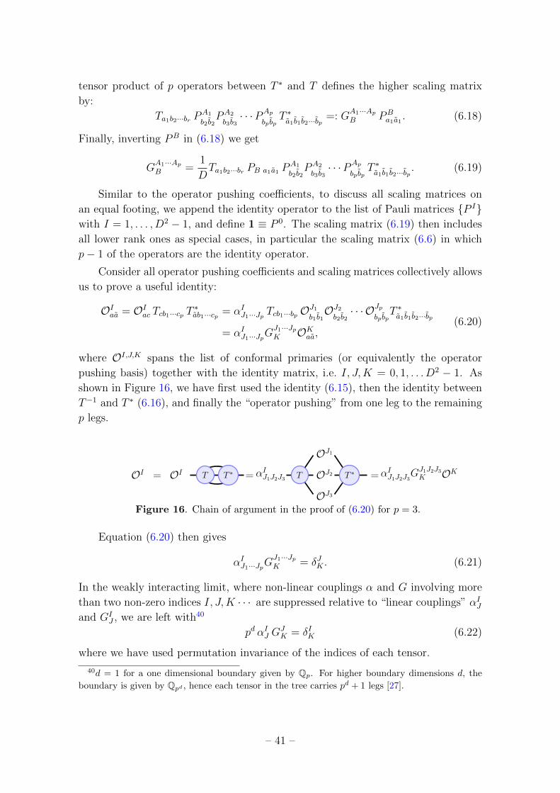
tensor product of p operators between T ∗ and T defines the higher scaling matrix

by:

Ta1b2···br PA1

b2b2PA2

b3b3· · ·PAp

bpbpT ∗a1b1b2···bp =: G

A1···ApB PB

a1a1. (6.18)

Finally, inverting PB in (6.18) we get

GA1···ApB =

1

DTa1b2···br PB a1a1 P

A1

b2b2PA2

b3b3· · ·PAp

bpbpT ∗a1b1b2···bp . (6.19)

Similar to the operator pushing coefficients, to discuss all scaling matrices on

an equal footing, we append the identity operator to the list of Pauli matrices {P I}with I = 1, . . . , D2 − 1, and define 1 ≡ P 0. The scaling matrix (6.19) then includes

all lower rank ones as special cases, in particular the scaling matrix (6.6) in which

p− 1 of the operators are the identity operator.

Consider all operator pushing coefficients and scaling matrices collectively allows

us to prove a useful identity:

OIaa = OIac Tcb1···cp T ∗ab1···cp = αIJ1···Jp Tcb1···bp OJ1b1b1OJ2b2b2· · · OJp

bpbpT ∗a1b1b2···bp

= αIJ1···JpGJ1···JpK OKaa,

(6.20)

where OI,J,K spans the list of conformal primaries (or equivalently the operator

pushing basis) together with the identity matrix, i.e. I, J,K = 0, 1, . . . D2 − 1. As

shown in Figure 16, we have first used the identity (6.15), then the identity between

T−1 and T ∗ (6.16), and finally the “operator pushing” from one leg to the remaining

p legs.

OI = OI = αIJ1J2J3

OJ1

OJ2

OJ3

=αIJ1J2J3

GJ1J2J3K OKT T ∗ T T ∗

Figure 16. Chain of argument in the proof of (6.20) for p = 3.

Equation (6.20) then gives

αIJ1···JpGJ1···JpK = δJK . (6.21)

In the weakly interacting limit, where non-linear couplings α and G involving more

than two non-zero indices I, J,K · · · are suppressed relative to “linear couplings” αIJand GI

J , we are left with40

pd αIJ GJK = δIK (6.22)

where we have used permutation invariance of the indices of each tensor.

40d = 1 for a one dimensional boundary given by Qp. For higher boundary dimensions d, the

boundary is given by Qpd , hence each tensor in the tree carries pd + 1 legs [27].

– 41 –

Diagonalizing (6.22) thus gives a relation between the eigenvalues λI ≡ p−σI of

the operator pushing matrix α, and the eigenvalue p−∆I of the scaling matrix G:

σI + ∆I = d (6.23)

which is precisely the relation between the conformal weights of the normalizable

and non-normalizable solutions of the free KG equation of bulk scalar fields. We

emphasize again that this relation emerges automatically in the tensor network.

7 Summary and Discussion

In this paper, we examined the tensor network/geometry correspondence in further

detail. Our aim was to read off a bulk interacting theory by inspecting the properties

of constituent tensors in the tensor network. This was done via two routes. First

by inspecting tensor identities satisfied by individual tensors, one can expand any

bulk operator in terms of a sum over boundary operators. By organizing the sum

systematically, each term acquires an interpretation as a Witten-like diagram in

the bulk, in direct correspondence with the HKLL relation found in the AdS/CFT

correspondence. This also allowed us to read off the field content in the bulk, and

determine the masses of these fields and their interaction couplings.

Then we applied our methods in a specific context — the p-adic AdS/CFT

correspondence. We constructed a tensor network based on the Bruhat-Tits tree,

and demonstrated that our method recovers the HKLL relation appropriate for p-

adic AdS/CFT. With the bulk isometries exactly matching the boundary symmetries

SL(2,Qp), it implied extra physical requirements on the constituent tensors. These

physical constraints allow us to compute boundary correlation functions exactly.

Once again, bulk Witten diagrams emerge, from which one can read off the field

content and interaction couplings. We demonstrated that in the “free field” limit

in the bulk, the correlation functions follow from non-normalizable bulk-boundary

propagators, as opposed to the normalizable ones that feature in the HKLL relation.

Moreover their scaling behaviours are related in precisely the same way as in the

AdS/CFT dictionary, a relation now derived based purely on properties of the tensor

network. It gives strong quantitative support that the tensor network is an explicit

embodiment of the AdS/CFT correspondence.

Unlike the construction of MERA, we did not demand from the very beginning

that T should be a unitary or isometry, although a very similar condition (6.15)

was later imposed for other physical requirements. A priori, there is no reason

that the constituent tensors of a tensor network should be unitaries or isometries.

This was imposed for efficient numerics. As far as a tensor network construction

of wave-function is concerned, the only physically relevant condition is to provide

as accurate an approximation as possible to the actual wave-function after auxiliary

– 42 –

indices are contracted. A “stochastic MERA” where all tensors take only positive

definite elements was recently constructed in [69].

It was noted in [26] that the tree tensor networks do not recover the Ryu-

Takayanagi formula. In other words, the length of the geodesic through the Bruhat-

Tits tree connecting two given end points at the boundary in general does not give

the entanglement entropy of the region bounded by the two points. Given that a

tree tensor network in fact produces the correct correlation functions, it suggests that

this is in fact a feature of p-adic CFT. We also commented on the precise relation-

ship between the wavelet transform and the AdS/CFT correspondence. Beyond its

philosophical value, the relationship provides a guiding principle for future attempts

at constructing tensor networks that are dual to some target (p-adic) CFT’s.

Before we close our summary, we note that there is one potential confusion

concerning the signature of the theory. In the usual discussion of the tensor network,

such as the MERA and the MPSs, they are descriptions of wavefunctions, which

are defined on a given time slice. In the p-adic version of AdS/CFT [26, 27], the

construction is a generalization of the Euclidean version of AdS/CFT. How then

should the tensor network be understood in this case?

To understand what happens, we recall works in the tensor network literature

where classical partition functions of statistical models admit a tensor network de-

scription, see for example [59, 60]. These tensor network representations of partition

functions, which are equivalent to Euclidean path-integrals of the quantum model

in one higher dimension, can also be coarse grained, which are linear maps of the

constituent tensors. If every step of the coarse graining is kept so that those linear

maps form layers of tensors in an extra dimension, we obtain a tensor network in one

extra dimension.

In other words, there is no mystery about the Euclidean version of the tensor net-

work/geometry correspondence. It would have the same form as MERA except that

what were previously physical dangling legs are now contracted among themselves

in the Euclidean path-integral. The bulk operator boundary operator reconstruction

is clearly independent of whether the boundary layers of legs are contracted among

themselves. We acknowledge that the computation of the correlation functions as

they are discussed in the current paper is rooted in the wave-function interpretation.

There is some tension in directly interpreting the tensor network as a generating

function of correlation functions. This however can be resolved by modifying our

tensor network into a form that is more readily interpretable as a path-integral. We

have made progress in this direction, and will report an alternative construction in

a future publication.

The current work is only the first step in elucidating the relation between tensor

networks and the AdS/CFT correspondence. We list some of the imminent questions

and generalizations in the following.

– 43 –

7.1 Implication to p-adic AdS/CFT

One reason that p-adic AdS/CFT is much less developed than the real version is

that there hasn’t been a well-defined, but non-trivial, “p-adic CFT”. With recent

developments [61, 62], the situation is quickly evolving. One of the main difficulties

that remain intriguing is that the ordinary derivative ∂z of the real case does not

exist for the p-adic field Qp. To proceed, there are two alternatives. One is to use

the “Vladimirov derivative”:

Dpf(x) ≡∫Qpdyf(y)− f(x)

|y − x|2p(7.1)

which defines the derivative via integration, and hence can be regarded as the p-adic

analogue of Cauchy’s contour integral in complex analysis. The resulting field theory

with a Lagrangian based on the “Vladimirov derivative” is therefore highly non-local

[63–65].

The other choice is to simply forgo the use of derivative, as in [50]. The “p-adic

CFT” defined this way would have only primary fields (defined using global SL(2,Qp)

as in (4.26)), and no descendants. The unitary condition is then automatically

satisfied and therefore cannot impose any constraints on the conformal weights of

allowed primaries. In fact, the form of all correlation functions is fixed and the

crossing symmetry is automatically satisfied. Therefore it also cannot impose any

constraints on the allowed primaries.41

With the result of the present paper, we can regard the tensor network living

on the Bruhat-Tits tree as a concrete realization of a “p-adic CFT”, with different

choices of the tensors corresponding to different matter content and interaction cou-

plings. Since a priori, any conformal dimension is allowed, and we do not need the

derivative or Lagrangian to define the theory, this is more in line with the second,

more algebraic, approach.

This then allows us to go beyond the free massless scalar. The next simplest

example would be the WN,k minimal model,42 which also has the benefit that it is

dual, by a weak/weak AdS/CFT correspondence, to a bulk higher spin gravity [66].

The existence of a weakly-coupled bulk dual living on the Bruhat-Tits tree then

imposes additional constraints on the boundary “p-adic CFT”. This is currently

under investigation.

41The modular invariance on higher genus Riemann surfaces might impose more constraints but

this has not been studied.42Tensor networks have been used to study the Ising model and three-state Potts model in the

real case in [59].

– 44 –

7.2 Further explorations in tensor networks

In this paper, we have studied very specific types of graphs. Namely they are un-

weighted graphs with a fixed valency. Our language should admit generalizations to

more general types of graphs. Let us comment briefly on two interesting extensions.

• For tree graphs with multiple valency, it can be described by a substitution

matrix. A substitution matrix M is a N ×N dimensional matrix, where N is

the number of different species, and Mij is the number of descendants belonging

to vertices of type j branching out from a vertex of type i . For example, if we

have only two kinds of vertices, we have

M =

(a b

c d

)(7.2)

where the matrix elements are positive integers. One solution to the (un-

weighted) graph Laplacian is

GO(a) = Nhmkn, (7.3)

where N is some suitable normalization and m + n = d(a,O), which is the

distance between a node a and the root of the graph O.43 To satisfy the graph

Laplacian equation with the same mass, we need to put in an extra constraint

so that the function satisfies the same equation independently of the type of

node the Laplacian acts on. The constraint is given by

ch+ dk +1

k− (c+ d+ 1) = ah+ bk +

1

h− (a+ b+ 1). (7.4)

It is not yet clear what such constraints could mean as far as the bulk interacting

theory is concerned. It should be studied systematically.

• Another generalization is to include weighted graphs. In this paper, we have

assumed that the network is a homogenous network and preserves as much

symmetry as the graph. In general when we start discussing fluctuations around

a background, then it seems natural that different edges should in general have

different weights. A first step has been taken in [28], where the weights are

interpreted as metric fluctuations. The Laplacian also depends on these weights

by

�φ(v) =∑u∼v

Juv(φ(u)− φ(v)), (7.5)

where Juv is the weight on the edge connecting the vertices u and v. It is an

important question to understand how these degrees of freedom emerge from

the tensor network.

43Roughly speaking, a rooted tree contains a special point from which the tree grows outwards.

– 45 –

• Time dependent evolution of the wavefunctions and dynamics in the bulk.

While a wavefunction can be evolved using any Hamiltonian that acts on the

boundary legs, it is not clear whether we can interpret that evolution as some

local dynamics of bulk degrees of freedom.

Apart from these generalizations, there are other important questions. In par-

ticular, it is evident that to recover a bulk theory that can be interpreted as a local

interacting theory, there are many constraints that need to be imposed on the tensors.

It is necessary to study these constraints systematically, and ask for the minimal set

of data needed to define the bulk theory. Such a discussion is pertinent to under-

standing when a large gap in conformal dimension is emerging, which is an essential

condition for the emergence of a semi-classical and local holographic dual [67].

Second, we need a theory of gravity in the bulk, and to that end, we need to

find a systematic way to describe fields carrying spin. As far as gravity is concerned,

one way to identify fluctuations of these tensors with gravitational excitations is

based on diffeomorphism. The idea is that the bulk graviton is supposedly dual

to the boundary stress tensor. One could therefore ask the following question: for

a given local diffeomorphism at the boundary, such as a local translation that can

be effected by inserting the (exponentiated) stress tensor ei∫dx ε(x)T0x , we can look

for the corresponding transformation in the bulk that would have (approximately)

the same effect. This would recover δgµν according to the Tµν inserted. The bulk

transformation in general corresponds to the exchange of edges (which is particularly

apparent in the case of a tree). It thus fits with a metric carrying two indices. This

is currently under investigation.

Last but not least, as we already mentioned in section 2.3, recovering bulk dy-

namics from boundary dynamics is an extremely important question. We hope to

return to these issues in the near future.

Acknowledgements

We are grateful to Olof Ahlen, Sumit Das, Muxin Han, Thomas Hartman, Matthias

Gaberdiel, Zheng-cheng Gu, Feng-li Lin, Hong Liu, Ezer Melzer, Mukund Ranga-

mani, Alfred Shapere, Wei Song, Aninda Sinha, and Yichao Tian for helpful discus-

sions and correspondences. We especially thank Feng-li Lin for teaching us about

wavelets and their recent implementation in tensor networks. AB thanks the Centre

for Theoretical Physics at MIT, Department of Physics and Astronomy at U. of Ken-

tucky, Physics Departments at UC Davis, UCSD, UIUC and Cornell for hospitality.

AB and LYH thank ITP-Chinese Academy of Sciences, and WL thanks the Physics

Department of Fudan University, for hospitality during various stages of this work.

We thank support from the Thousand Young Talents Program.

– 46 –

Appendix

A Lattice construction of Bruhat-Tits tree

Since Hp has a discrete topology, we cannot simply give Hp the coordinate zp =

xp + i yp in which xp ∈ Qp and yp ∈ Qp+, and write down the PGL(2,Qp) invariant

metric on it. However, the coset expression (4.10) suggests that one can construct it

in terms of equivalence classes of lattices in Qp ⊗Qp.

A lattice in Qp ⊗Qp generated by basis vectors (~f,~g)

~f ≡(f1

f2

)~g ≡

(g1

g2

)with fi, gi ∈ Qp (A.1)

which satisfy ~f 6= c~g for ∀c ∈ Qp is defined as44

〈~f,~g〉 ≡ {a~f + b~g | a, b ∈ Zp}. (A.2)

A PGL(2,Qp) transformation acts on the lattice via

〈~f,~g〉 → 〈γ · ~f, γ · ~g〉 with γ =

(a b

c d

)∈ PGL(2,Qp). (A.3)

The numerator PGL(2,Qp) in (4.10) acts transitively on the space of lattices in

Qp ⊗ Qp, and the denominator PGL(2,Zp) is the stabilizer of the integer lattice

Zp ⊗ Zp. Therefore Hp defined as coset (4.10) is identical to the set of equivalence

classes {Λ} of lattices in Qp⊗Qp, where two lattices are equivalent, 〈~f,~g〉 ∼ 〈~f ′, ~g′〉,iff

(~f ′, ~g′) = (Γ · ~f,Γ · ~g) with Γ ∈ PGL(2,Zp) (A.4)

Note that since we use PGL instead of SL, we have

〈~f,~g〉 ∼ λ〈~f,~g〉 with λ ∈ Q∗p (A.5)

We denote the equivalence class of a lattice generated by (f, g) as 〈〈f, g〉〉.Now we are ready to define the metric on Hp, i.e. the distance between two points

in Hp, i.e. two equivalence classes of lattices Λ and Λ′ in Qp ⊗ Qp. First, Λ and Λ′

are defined as incident (i.e. directly connected) if and only if45

pΛ ⊂ Λ′ ⊂ Λ. (A.6)

44Here we see an important difference between the lattices on R ⊗ R and the p-adic lattices.

Since a, b ∈ Zp (the unit ball inside Qp), which is continuous, the p-adic lattices form a continuum,

whereas the R⊗ R lattices are discrete.45To check that this definition is reflective, we note that since pΛ is equivalent to Λ, multiplying

the equation above by p gives pΛ′ ⊂ Λ ⊂ Λ′.

– 47 –

We connect such a pair of nodes by an edge, which has distance d(Λ,Λ′) = 1. One

can immediately check that each node has exactly (p + 1) nearest neighbors, i.e.

that Hp has the topology of an infinite (p + 1)-valent tree (shown in Fig. 6(c) for

p = 2), instead of a Qp ⊗ Qp continuum. Figure 17 shows the Bruhat-Tits tree for

p = 2. Then the distance between any two points is defined as the number of edges

connecting them, which is invariant under PGL(2,Qp).

0

x ∈ Qp

p2

p1

p0(f, g)

(f, 2g)

pm

(2f, g)

(4f, g)

(2f, g + f)

Figure 17. Bruhat-Tits tree for p = 2. Here f ≡ ~f0 and g ≡ ~g0.

For the real case, it is easy to visualize the relation between the upper half plane

H and its boundary R. In the coordinate z = x+i y (with which the hyperbolic metric

is ds2 = 1y2

(dx2 + dy2)), taking limy→0 gives the boundary point x and increasing y

moves deeper in the bulk. An SL(2,R) action on a point z = x + i y on H would

induce the same action on its boundary point x, see (4.25). In particular, in the study

of holography, the constant y = ε � 1 line is taken to be the cut-off surface. (The

choice of the cut-off surface is particularly crucial in the tensor network construction.)

What is the analogous situation for the p-adic case here?

The lattice construction earlier only gives the topology of the tree. We would like

to have a good coordinate system on the Bruhat-Tits tree Hp such that its boundary

is the p-adic field Qp, and the PGL(2,Qp) action on a vertex in the bulk Hp induces

the same action on its boundary point. In particular, the natural cut-off surface from

this coordinate system behaves well in the tensor network construction.

To fix a coordinate system in Hp, first choose the origin O. Since the tree is

infinite and homogeneous, we can choose an arbitrary point as the origin O. We

can then use the isomorphism PGL(2,Qp) to make O the equivalence class of integer

– 48 –

lattice, i.e. its generators are

O ≡ 〈〈~f0, ~g0〉〉 with ~f0 ≡(

1

0

)~g0 ≡

(0

1

). (A.7)

One first checks that the (p+ 1) neighbors of O are

〈〈(

1

0

),

(0

p

)〉〉 〈〈

(p

0

),

(n

1

)〉〉 with n = 0, 1, . . . , p− 1. (A.8)

Note that these are precisely the neighbors that would arise when applying the Hecke

operator

Tp(m) = m ·(

1 0

0 p

)+m ·

p−1∑n=0

(p n

0 1

)(A.9)

on the node 〈〈f0, g0〉〉. Now we use the projective equivalence (A.5) to fix the second

vector g to g0, i.e. rewrite the first node in (A.8) into 〈〈(

1p

0

),

(0

1

)〉〉.

Applying Hecke operator iteratively then generates the entire tree, with all nodes

having the form

〈〈(pm

0

),

(x(m)

1

)〉〉 x(m) =

m−1∑n=−N

anpn an ∈ Fp, (A.10)

where we have used the projective equivalence (A.5) to fix g2 = 1. Figure 17 shows

the Bruhat-Tits tree for p = 2, with the coordinate system (4.12). Note that since

x(m) truncates at pm, we can think of pm as giving the accuracy level of a p-adic

number x(m), i.e. the node (4.12) represents the equivalence class x(m) + pmZp.

B Basics of p-adic analysis

In this appendix we review some basics on p-adic integration, p-adic Fourier trans-

form, and p-adic wavelet transform, which will be needed when we discuss the bulk

operator reconstruction in p-adic AdS/CFT in section 5.2. For more on p-adic anal-

ysis see the textbook [38]. The summary on p-adic integration and Fourier transform

here follows mainly the chapter 3 of [68].

B.1 p-adic integration

The integration measure is not unique. There are several commonly used measures

for p-adic integration. First, the additive measure dx over the Qp line is defined by

demanding the following translation and scaling behavior

d(x+ a) = dx and d(ax) = |a|p dx (B.1)

– 49 –

Usually it is normalized over the “unit ball” (defined in (4.9))∫Zpdx = 1 (B.2)

Not surprisingly, the integration over the entire Qp using the additive measure dx

diverges. The multiplicative measure d×x over Q×p can be defined by

d×(x) ≡ p

p− 1

dx

|x|p(B.3)

which satisfies d×(ax) = d×x and∫Z×pd×x = 1. Finally, the Patterson-Sullivan

measure dµ(x) over P1(Qp) is defined as

dµ(x) =

{dx x ∈ Zpdx|x|2p otherwise

(B.4)

The distance as seen by this measure agrees with the one computed by counting

steps in the BT tree.

B.2 p-adic Fourier transform

To define the p-adic Fourier transformation, we need the analogue of e2πikx, i.e. the

additive characters on Qp. This is defined as46

χk(x) ≡ e−2πi [kx] (B.5)

where [x] is the “fractional part” of the p-adic number x, defined as

[x] ≡−1∑

n=−Nanp

n (B.6)

and [x] = 0 for x ∈ Zp, i.e. |x|p ≤ 1 (hence the name “fractional part”). It is easy

to check that χk(x)χk(y) = χk(x + y) and |χk(x)|p = 1. Integrating the additive

character χk(x) over the unit ball Zp gives the characteristic function γ(k) of Zp in

Qp: ∫Zpdx e−2πi [kx] ≡ γ(k) =

{1 k ∈ Zp0 otherwise

(B.7)

Note that both the additive character χk and the characteristic function γ(k) of Zpin Qp are locally constant functions.47

46The sign difference in the exponent between the real character and the p-adic one is important

for constructing the adelic product.47As a contrast, recall that for a function from R to R, “locally constant” implies “constant”.

– 50 –

For the study of the p-adic Fourier transform, we summarize a few useful inte-

grals, which are interesting in their own right. First, the integration over bigger balls

pnZp gives the characteristic function of pnZp in Qp, i.e. γ(pnk):∫pnZp

dx e−2πi [kx] =1

pnγ(pnk) (B.8)

From this we can compute the integration over “shells”

∫pnUp

dx e−2πi [kx] =

p−1pn+1 |k|p < pn+1

−1pn+1 |k|p = pn+1

0 |k|p > pn+1

(B.9)

where Up is the “unit sphere” of p-adic numbers defined in (4.8). This in turn gives∫Qp\Zp

dx e−2πi [kx] = −γ(k) (B.10)

The p-adic functions that allow a well-defined (i.e. invertible) Fourier transform

are locally constant (i.e. constant within each pnZ×p ) functions with compact support

or sufficiently fast asymptotic decay. The p-adic Fourier transform and its inverse is

then

f(k) =

∫Qpdx f(x)e−2πi[kx] and f(x) =

∫Qpdk f(k)e2πi[kx] (B.11)

The characteristic function γ(x) of Zp in Qp is invariant under the Fourier trans-

form, i.e.

γ(x) = γ(x) (B.12)

hence γ(x) is also called p-adic Gaussian.

C Some examples

C.1 GHZ tensor

One very simple example that satisfies permutation invariance and (6.15) at the same

time is given by the GHZ state, which can be defined for arbitrary valency r and

bond dimension D. The only non-vanishing components are given by

Ta···a = 1, 1 ≤ a ≤ D. (C.1)

For simplicity, let us consider D = 2 and r = 3 explicitly. There, the Pauli basis

is simply given by the Pauli matrices σx,y,z. Therefore we can check that only σz has

– 51 –

a linear term under operator pushing. The linear pushing coefficient defined in (3.7)

and the scaling relation defined in (6.6) are given by

αZZ =1

2=GZZ

2. (C.2)

This means that σz has scaling dimension ∆ = 0. In this case, the cubic coupling

αABC and GABC vanish. We can then explicitly see that 2αZZ × GZ

Z = 1, satisfying

(6.22).

The other two Pauli operators σx,y however, have infinite scaling dimension.

The GHZ state for general dimensions generates unfortunately either operators with

vanishing or infinite scaling dimensions. Despite not having a physical spectrum, it

does illustrate in very simple terms the ideas described in this paper.

C.2 Random tensors

Consider the coupling constants in a generic tensor network built from r leg tensors

with large bond dimensions D. We can use Haar weighted random tensors to estimate

how the non-linear couplings scale with D in the large D limit.

First, we compute two point functions to appropriately normalize the operators.

From the requirement that (6.15), we require

N 4tr(|T 〉〈T | ⊗ |T 〉〈T |) = D. (C.3)

Now using results from [20], we have

tr(|T 〉〈T | ⊗ |T 〉〈T |) = trI + F

D2r +Dr= 1, (C.4)

where F is the swap operator swapping the two copies i.e. F|T1〉 ⊗ T2〉 = |T2〉 ⊗ T1〉.Therefore N =

√D.

Then

(GAB)2 =

D2

D2

tr((PA2)tr((PB2

)(tr(1)D−2)

D2r +Dr∼ 1

Dr. (C.5)

On the other hand, three point couplings are given by exactly the same value. i.e.

(GABC)2 =

1

Dr. (C.6)

We therefore have(GA

BC)2

(GAB

2)3/2

=D−r

D−3r/2= Dr/2, (C.7)

which diverges in the large D limit, as expected.

– 52 –

D Bulk operator reconstruction in the vicinity of the perfect

code

In this appendix, we will demonstrate how the discussion of HKLL-like relations and

fusion matrices in equation (3.10) are related to the discussion in [21]. To that end,

like [21], we will have to work in the limit where every tensor is close to being a

perfect tensor. Recall that a perfect tensor is one satisfying (2.10). Now we will

consider tensors at each site taking the form

T = T + ε t , (D.1)

where T is a perfect tensor, and t is some arbitrary tensor and ε an infinitesimal

parameter.

We would like to extract the index αAB1···Bn . This can be obtained by multiplying

both sides by the set of out operators ⊗iPBi , and then taking the trace. This is

depicted in Figure 18.

αAB1..Bn

1

Dr−1=

PA

PB1

PBn

···

··· r − 1− n

T−1 T

Figure 18. This depicts how the expansion coefficients αAB1···Bn can be computed.

To order ε0, T−1 is indeed just T ∗. Using (2.10) and (3.6), one can readily show

that the first coefficient that would show up at ε0 has to be αAB1,···Br/2 . This is indeed

the case in every explicit example of a perfect tensor.

E Boundary global Space (time) symmetry via tensor trans-

formations

In this appendix, we would like to make explicit how the spacetime symmetries are

realized via tensor transformations. We note that the tensor network has so far only

been used as a description of wavefunctions. Therefore symmetries related to boosts

are not explicitly respected. However, if we focus on space-like symmetries, or take

the tensor network as a Euclidean bulk, then the statement of symmetries can be

taken as follows.

For a state invariant under some space-symmetry transformation g, it means

g|Ψ〉 = |Ψ〉. (E.1)

For example, g could correspond to quantum operators implementing translations,

rotation or scaling in a CFT. The state |Ψ〉 however is constructed from contraction

– 53 –

of tensors in a network. This means that the description of the state in terms of

these tensors involves a large amount of redundancy — any contracted leg between

two neighboring tensors T I and T J can be rotated by a unitary transformation:48

· · ·T IaαT Jα b · · · = · · ·T IaαUαβU †βγT Jγ b · · · . (E.2)

This transformation U is often also referred to as a gauge symmetry in the standard

tensor network literature.

Therefore the symmetry transformation is defined up to a gauge transformation

gabT (v)b,i′e1 ,i′e2,··· = T (g.v)a,ie1 ,ie2 ,···W

gie1 ,i

′e1

(e1)W gie2 ,i

′e2

(e2) · · · . (E.3)

Here we made the distinction between the symmetry transformation of the CFT

wavefunction, denoted g, and the geometric transformation g of the tensor network

graph. In a holographic type tensor network, this is very interesting. In addition

to inducing gauge transformations, the tensor at the top level has moved elsewhere.

It means that the tensor on the RHS of the equation has to move to a different

vertex g.v, which is precisely one dictated by the action of the transitive action of

the symmetry in the bulk. In the case of the Bruhat-Tits tree, g.v would be defined

by equation (4.19).

The above equation only considers the simple situation in which motion of the

vertices in the bulk suffices. This is the case if we impose also permutation invariance

of all the legs of an individual tensor. In general, the symmetry transformation might

also involve the permutation between legs. This would require a systematic study. In

the following, we will only briefly illustrate this proposal in a 3-qutrit code discussed

also in [19].

It is interesting to contrast space-symmetries with global internal symmetries.

In the latter, it is known in the literature that it is convenient to impose invariance

of individual tensors under the action of the global symmetry group. As a result, the

global symmetry is enhanced to a gauge symmetry in the bulk, precisely as expected

in the AdS/CFT dictionary. Here, the “gauge transformations” appearing in the

RHS of (E.3) are probably related to the bulk diffeomorphism. But it probably does

not recover the full scope of diffeo-invariance of the bulk. A proper description would

amount to recovering all the redundancy in the tensor network, and subsequently the

closest analogue of gravity in the discrete space-time. This is certainly beyond the

scope of the current paper, and we will restrict our attention to global bulk isometries.

E.1 Example using the 3-qutrit code

We now study the example of the pentagon code. We will consider two different

types of wavefunctions to illustrate the above point. For concreteness, one can take

48We use capital Latin letters to label tensors on individual sites of the network, Greek letters

for contracted indices, and small Latin letter for boundary legs.

– 54 –

the 3-qutrit code [19]. Then each tensor T Iαβγ has 4 indices, each taking 3 values

{0, 1, 2}. The index I is treated as a bulk index. To illustrate how the symmetry

acts, we can take these tensors to populate the 2-adic tree.

Consider for simplicity performing a scaling transformation. As described in

section 4.3.1, this corresponds to a translation of branches along the main branch,

see figure 7. Therefore, a scaling transformation of the wave function would corre-

spond to moving the tensors in exactly the same fashion as the nodes of the tree,

while preserving the orientation of each tensor (if they are not already permutation

invariant).

Practically, to effect a translation in this tree, we can make use of the following

operator:

T =∏

l,<vil ,vil+1>

(Ivil ⊗ Ivil+1 +D2−1∑M=1

(P vlM ⊗ P

vil+1

M )), (E.4)

where the superscript v denotes the site index. PvilM are the generalized Pauli matrices

as described in (3.6) and Iv is the identity matrix that acts on the bulk index of the

tensor located at vertex v. For the 3- qutrit code therefore, D = 3. Each term in the

product exchanges the vil site and the vil+1 site. The product runs over the sequence

of vertices, i.e. the set of vertices {vil} which transforms as vil → vil+1, and where

l is a “layer” index. Translation is effected within each layer l. The wave function

generated by this transformation is one in which the boundary sites are transformed

according to x→ px.

References

[1] G. ’t Hooft, “Dimensional reduction in quantum gravity,” Salamfest 1993:0284-296

[gr-qc/9310026];

[2] L. Susskind, “The World as a hologram,” J. Math. Phys. 36, 6377 (1995)

[hep-th/9409089].

[3] J. M. Maldacena, “The Large N limit of superconformal field theories and

supergravity,” Int. J. Theor. Phys. 38 (1999) 1113 [arXiv:hep-th/9711200].

[4] E. Bianchi and R. C. Myers, “On the Architecture of Spacetime Geometry,” Class.

Quant. Grav. 31, 214002 (2014) [arXiv:1212.5183 [hep-th]].

[5] B. Swingle, “Constructing holographic spacetimes using entanglement

renormalization,” [arXiv:1209.3304 [hep-th]].

[6] B. Czech, G. Evenbly, L. Lamprou, S. McCandlish, X. L. Qi, J. Sully and G. Vidal,

“Tensor network quotient takes the vacuum to the thermal state,” Phys. Rev. B 94,

no. 8, 085101 (2016) [arXiv:1510.07637 [cond-mat.str-el]].

[7] B. Czech, L. Lamprou, S. McCandlish and J. Sully, “Tensor Networks from

Kinematic Space,” JHEP 1607, 100 (2016) [arXiv:1512.01548 [hep-th]].

– 55 –

[8] M. Nozaki, S. Ryu and T. Takayanagi, “Holographic Geometry of Entanglement

Renormalization in Quantum Field Theories,” JHEP 1210 (2012) 193

[arXiv:1208.3469 [hep-th]].

[9] A. Mollabashi, M. Nozaki, S. Ryu and T. Takayanagi, “Holographic Geometry of

cMERA for Quantum Quenches and Finite Temperature,” JHEP 1403 (2014) 098

[arXiv:1311.6095 [hep-th]].

[10] M. Miyaji and T. Takayanagi, “Surface/State Correspondence as a Generalized

Holography,” PTEP 2015, no. 7, 073B03 (2015) [arXiv:1503.03542 [hep-th]].

[11] M. Miyaji, T. Numasawa, N. Shiba, T. Takayanagi and K. Watanabe, “Continuous

Multiscale Entanglement Renormalization Ansatz as Holographic Surface-State

Correspondence,” Phys. Rev. Lett. 115, no. 17, 171602 (2015) [arXiv:1506.01353

[hep-th]].

[12] N. Bao, C. Cao, S. M. Carroll, A. Chatwin-Davies, N. Hunter-Jones, J. Pollack and

G. N. Remmen, “Consistency conditions for an AdS multiscale entanglement

renormalization ansatz correspondence,” Phys. Rev. D 91, no. 12, 125036 (2015)

[arXiv:1504.06632 [hep-th]].

[13] A. Almheiri, X. Dong and D. Harlow, “Bulk Locality and Quantum Error

Correction in AdS/CFT,” JHEP 1504 (2015) 163 [arXiv:1411.7041 [hep-th]].

[14] E. Mintun, J. Polchinski and V. Rosenhaus, “Bulk-Boundary Duality, Gauge

Invariance, and Quantum Error Corrections,” Phys. Rev. Lett. 115, no. 15, 151601

(2015) [arXiv:1501.06577 [hep-th]].

[15] E. M. Brehm and B. Richter, “Classical Holographic Codes,” Phys. Rev. D 96, no.

6, 066005 (2017) [arXiv:1609.03560 [hep-th]].

[16] M. Miyaji, T. Takayanagi and K. Watanabe, “From Path Integrals to Tensor

Networks for AdS/CFT,” Phys. Rev. D 95, no. 6, 066004 (2017)

[arXiv:1609.04645 [hep-th]].

[17] B. Czech, P. H. Nguyen and S. Swaminathan, “A defect in holographic

interpretations of tensor networks,” JHEP 1703, 090 (2017) [arXiv:1612.05698

[hep-th]].

[18] A. Peach and S. F. Ross, “Tensor Network Models of Multiboundary Wormholes,”

Class. Quant. Grav. 34, no. 10, 105011 (2017) arXiv:1702.05984 [hep-th].

[19] F. Pastawski, B. Yoshida, D. Harlow and J. Preskill, “Holographic quantum

error-correcting codes: Toy models for the bulk/boundary correspondence,” JHEP

1506, 149 (2015) [arXiv:1503.06237 [hep-th]].

[20] P. Hayden, S. Nezami, X. L. Qi, N. Thomas, M. Walter and Z. Yang, “Holographic

duality from random tensor networks,” JHEP 1611, 009 (2016) [arXiv:1601.01694

[hep-th]].

[21] A. Bhattacharyya, Z. S. Gao, L. Y. Hung and S. N. Liu, “Exploring the Tensor

– 56 –

Networks/AdS Correspondence,” JHEP 1608 (2016) 086 [arXiv:1606.00621

[hep-th]].

[22] M. Han and L. Y. Hung, “Loop Quantum Gravity, Exact Holographic Mapping, and

Holographic Entanglement Entropy,” Phys. Rev. D 95, no. 2, 024011 (2017)

[arXiv:1610.02134 [hep-th]].

[23] G. Chirco, D. Oriti and M. Zhang, “Group Field theory and Tensor Networks:

towards a Ryu-Takayanagi formula in full quantum gravity,” [arXiv:1701.01383

[gr-qc]].

[24] C. H. Lee and X. L. Qi, “Exact holographic mapping in free fermion systems,” Phys.

Rev. B 93, no. 3, 035112 (2016) [arXiv:1503.08592 [hep-th]].

[25] S. Singh and G. K. Brennen, “Holographic Construction of Quantum Field Theory

using Wavelets,” [arXiv:1606.05068 [quant-ph]].

[26] M. Heydeman, M. Marcolli, I. Saberi and B. Stoica, “Tensor Networks, p-adic

Fields, and Algebraic Curves: Arithmetic and the AdS3/CFT2 Correspondence,”

[arXiv:1605.07639 [hep-th]].

[27] S. S. Gubser, J. Knaute, S. Parikh, A. Samberg and P. Witaszczyk, “p-adic

AdS/CFT,” Commun. Math. Phys. (2017). [arXiv:1605.01061 [hep-th]].

[28] S. S. Gubser, M. Heydeman, C. Jepsen, M. Marcolli, S. Parikh, I. Saberi, B. Stoica

and B. Trundy, “Edge length dynamics on graphs with applications to p-adic

AdS/CFT,” [arXiv:1612.09580 [hep-th]].

[29] R. Orus, “A Practical Introduction to Tensor Networks: Matrix Product States and

Projected Entangled Pair States,” Annals Phys. 349 (2014) 117 [arXiv:1306.2164

[cond-mat.str-el]] .

[30] R. Orus, “Advances on Tensor Network Theory: Symmetries, Fermions,

Entanglement, and Holography,” Eur. Phys. J. B 87 (2014) 280 [arXiv:1407.6552

[cond-mat.str-el]].

[31] S. Ryu and T. Takayanagi, “Holographic derivation of entanglement entropy from

AdS/CFT,” Phys. Rev. Lett. 96 (2006) 181602 [hep-th/0603001].

[32] S. Ryu and T. Takayanagi, “Aspects of Holographic Entanglement Entropy,” JHEP

0608 (2006) 045 [hep-th/0605073].

[33] S. Singh and G. Vidal, “Symmetry protected entanglement renormalization,” Phys.

Rev. B 88, no. 12, 121108 (2013) [arXiv:1303.6716 [cond-mat.str-el]].

[34] A. Hamilton, D. N. Kabat, G. Lifschytz and D. A. Lowe, “Local bulk operators in

AdS/CFT: A Holographic description of the black hole interior,” Phys. Rev. D 75,

106001 (2007) [arXiv:hep-th/0612053].

[35] A. Hamilton, D. N. Kabat, G. Lifschytz and D. A. Lowe, “Local bulk operators in

AdS/CFT: A Boundary view of horizons and locality,” Phys. Rev. D 73, 086003

(2006) [arXiv:hep-th/0506118].

– 57 –

[36] D. Kabat, G. Lifschytz and D. A. Lowe, “Constructing local bulk observables in

interacting AdS/CFT,” Phys. Rev. D 83, 106009 (2011) [arXiv:1102.2910

[hep-th]].

[37] J. E. Humphreys, ”Reflection Groups and Coxeter Groups,” Cambridge University

Press (1990).

[38] N. Koblitz, “p-adic Numbers, p-adic Analysis and Zeta-Functions,” 2nd edition,

Springer (1984).

[39] F. Q. Gouvea, “p-adic Numbers: An Introduction,” 2nd edition, Springer (1997).

[40] P. G. O. Freund and M. Olson, “Nonarchimedean Strings,” Phys. Lett. B 199, 186

(1987).

[41] L. Brekke and P. G. O. Freund, “p-adic numbers in physics,” Phys. Rept. 233, 1

(1993).

[42] L. Brekke, P. G. O. Freund, M. Olson and E. Witten, “Nonarchimedean String

Dynamics,” Nucl. Phys. B 302, 365 (1988).

[43] P. G. O. Freund and E. Witten, “Adelic String Amplitudes,” Phys. Lett. B 199

(1987) 191.

[44] B. Dragovich, “Zeta Strings,” [arXiv:hep-th/0703008].

[45] B. Dragovich, A. Y. Khrennikov, S. V. Kozyrev and I. V. Volovich, “On P-Adic

Mathematical Physics,” Anal. Appl. 1 (2009) 1 [arXiv:0904.4205 [math-ph]].

[46] Y. I. Manin and M. Marcolli, “Holography Principle and Arithmetic of Algebraic

Curves,” Adv. Theor. Math. Phys. 5 (2002) 617 [hep-th/0201036].

[47] A. Ostrowski, “Uber einige Losungen der Funktionalgleichung Ψ(x) ·Ψ(y) = Ψ(xy),”

Acta Mathematica 41 (1916) 271.

[48] F. Bruhat and J. Tits, “Groupes reductifs sur un corps local: I. Donnees radicielles

valuees,” Inst. Hautes Etudes Sci. Publ. Math. 41 (1972) 5.

[49] A. V. Zabrodin, “Nonarchimedean Strings and Bruhat-tits Trees,” Commun. Math.

Phys. 123, 463 (1989).

[50] E. Melzer, “Nonarchimedean Conformal Field Theories,” Int. J. Mod. Phys. A 4

(1989) 4877.

[51] F. R. K. Chung, “Spectral graph theory,” American Mathematical Soc., 1997.

[52] A. Hamilton, D. N. Kabat, G. Lifschytz and D. A. Lowe, “Holographic

representation of local bulk operators,” Phys. Rev. D 74, 066009 (2006)

[arXiv:hep-th/0606141].

[53] G. Brattle, “Wavelets and Renormalization”, World Scientific (1998)

[54] G. Evenbly and S. White, “Entanglement renormalization and wavelets” Phys. Rev.

Lett, 116 140403 (2016)

– 58 –

[55] D. K. Hammond, P. Vandergheynst and R. Gribonval, “ Wavelets on graphs via

spectral graph theory,” Applied and Computational Harmonic Analysis 30, no. 2,

129

[56] D. Harlow, S. H. Shenker, D. Stanford and L. Susskind, “Tree-like structure of

eternal inflation: A solvable model,” Phys. Rev. D 85, 063516 (2012)

[arXiv:1110.0496 [hep-th]].

[57] S. Albeverio and S. V. Kozyrev, “Coincidence of the continuous and discrete p-adic

wavelet transforms,” [arXiv:math-ph/0702010]

[58] R. Pfeifer, G. Evenbly and G. Vidal, “Entanglement renormalization, scale

invariance, and quantum criticality”, Phys. Rev. A, 79, 040301 [arXiv:0810.0580

[cond-mat.str-el]]

[59] S. Yang, Z. C. Gu and X. G. Wen, “Loop optimization for tensor network

renormalization”, Phys. Rev. Lett. 118 110504 (2017) [arXiv:1512.04938

[cond-mat.str-el]]

[60] G. Evenbly and G. Vidal, “Tensor Network Renormalization Yields the Multiscale

Entanglement Renormalization Ansatz”, Phys. Rev. Lett. 115, 200401

[arXiv:1502.05385 [cond-mat.str-el]]

[61] S. S. Gubser, C. Jepsen, S. Parikh and B. Trundy, “O(N) and O(N) and O(N),”

arXiv:1703.04202 [hep-th].

[62] S. S. Gubser, M. Heydeman, C. Jepsen, S. Parikh, I. Saberi, B. Stoica and

B. Trundy, “Signs of the time: Melonic theories over diverse number systems,”

arXiv:1707.01087 [hep-th].

[63] R. B. Zhang, “Lagrangian Formulation of Open and Closed p-adic Strings,” Phys.

Lett. B 209 (1988) 229.

[64] B. L. Spokoiny, “Quantum Geometry of Nonarchimedean Particles and Strings,”

Phys. Lett. B 208 (1988) 401.

[65] G. Parisi, “On P-Adic Functional Integrals,” Mod. Phys. Lett. A 3 (1988) 639.

[66] M. R. Gaberdiel and R. Gopakumar, “An AdS3 Dual for Minimal Model CFTs,”

Phys. Rev. D 83 (2011) 066007 [arXiv:1011.2986 [hep-th]].

[67] I. Heemskerk, J. Penedones, J. Polchinski and J. Sully, “Holography from Conformal

Field Theory,” JHEP 0910, 079 (2009) [arXiv:0907.0151 [hep-th]].

[68] P. Fleig, H. P. A. Gustafsson, A. Kleinschmidt and D. Persson, “Eisenstein Series

and Automorphic Representations,” [arXiv:1511.04265 [math.NT]].

[69] M. Bal, M. Marien, J. Haegeman, F. Verstraete, “Renormalization group flows of

Hamiltonians using tensor networks,” Phys. Rev. Lett. 118 250602 (2017)

– 59 –