Tensor-GMRES Method for Large Sparse

Systems of Nonlinear Equations

Dan Feng and Thomas H. Pulliam

The Research Institute for Advanced Computer Science is operated by Universities Space Research

Association, The American City Building, Suite 212, Columbia, MD 21044 (410)730-2656

Work reported herein was supported by NASA under contract NAS 2-13721 between NASA and the

Universities Space Research Association (USRA).

https://ntrs.nasa.gov/search.jsp?R=19940033144 2020-04-18T05:57:00+00:00Z

TENSOR-GMRES METHOD FOR LARGE SPARSE

SYSTEMS OF NONLINEAR EQUATIONS*

by

Dan Feng t and Thomas H. Pulliam _

*Work reported herein was supported by NASA under contract NAS 2-13721 between NASA and the

Universities Space Research Association (USRA).t Research Institute for Advanced Computer Science (RIACS), Mail Stop T20G-5, NASA Ames Research

Center, Moffett Field, CA 94035-1000, USA. (feng@riacs.edu)_Fluid Dynamics Division, Mail Stop T27B-1, NASA Ames Research Center, Moffett Field, CA 94035-

1000, USA. (puUiam@nas.nasa.gov)

Abstract

This paper introduces a tensor-Krylov method, the tensor-GMRES method, for large

sparse systems of nonlinear equations. This method is a coupling of tensor model forma-tion and solution techniques for nonlinear equations with Krylov subspace projection

techniques for unsymmetric systems of linear equations. Traditional tensor methods

for nonlinear equations are based on a quadratic model of the nonlinear function, astandard linear model augmented by a simple second order term. These methods are

shown to be significantly more efficient than standard methods both on nonsingular

problems and on problems where the Jacobian matrix at the solution is singular. A

major disadvantage of the traditional tensor methods is that the solution of the tensor

model requires the factorization of the Jacobian matrix, which may not be suitable for

problems where the Jacobian matrix is large and has a "bad" sparsity structure for anefficient factorization. We overcome this difficulty by forming and solving the tensor

model using an extension of a Newton-GMRES scheme. Like traditional tensor meth-

ods, we show that the new tensor method has significant computational advantages over

the analogous Newton counterpart. Consistent with Krylov subspace based methods,the new tensor method does not depend on the factorization of the Jacobian matrix.

As a matter of fact, the Jacobian matrix is never needed explicitly.

1 Introduction

This paper introduces a tensor-Krylov method for solving the nonlinear equations problem

given F : _N _., _}_N, find x. E _N such that F(x.) = O. (1.1)

Standard methods (such as Newton's method) widely used in practice for solving (1.1) are

iterative methods that base each iteration upon a linear model of F at the current point xc,

M(xc + d) = F(xc) + J_d, (1.2)

where d E _}_N and J_ E _N×N is either the current Jacobian matrix or an approximation

to it. When the size of J_ is moderate or the sparsity structure of Jc is favorable, many

effective ways of solving the linear model are based on the factorization of Jc (for example LU

factorization). However, for many real world problems (often arisen in numerical solution

of ODEs and PDEs), J_ is often large and has a sparsity structure that does not allow a

sparse factorization. The density of a full factorization would be so great that the storageof such a factorization would be impossible even on the most powerful computer available

today due to unavoidable massive fill-ins. An attractive alternative to solving the linear

model is the use of Krylov methods, such as the GMRES method, which does not require

the factorization of Jc. The distinct advantage of Krylov methods is their minimum storage

requirement and potential matrix-free implementations. Newton-like iteration schemes for

solving the nonlinear equations problem using Krylov subspace projection methods as an

inner linear solver are considered by many authors including Brown and Saad [5, 4], Chan

and Jackson [6], and Brown and Hindmarsh [3]. Their computational results show that

these methods can be quite effective for many classes of problems in the context of systems

of partial differential equations or ordinary differential equations.

The distinguishing feature of the Newton equation based algorithm is that if Ft(xc)

is Lipschitz continuous in a neighborhood containing the root x., F(x.) is nonsingular

and (1.2)is solved exactly (or to certain accuracy, e.g. see [4] for more details), then

the sequence of iterates produced converges locally and q-quadratically to x.. This means

eventual fast convergence in practice. However, Newton's (or Newton-like) method is not

usually quickly locally convergent, if F_(x.) is singular. This situation is analyzed and

acceleration techniques are suggested by many authors, including Reddien [23], Decker and

Kelley [8],[9],[10], Decker, Keller and Kelley [7], Kelley and Suresh [17], Griewank and

Osborne [15], and Griewank [14]. In summary, their papers show that when the Jacobian

at the solution has a null space of dimension one, then from good starting points, Newton's

method is locally Q-linearly convergent with constant converging to ½. The acceleration

techniques presented in these papers depend upon a priori knowledge that the problem is

singular.

Tensor methods for nonlinear equations introduced by Schnabel and Frank [26] are

intended to be efficient both for nonsingular problems and for problems with low rank

deficiency. These methods augment the standard linear model by a low rank second order

term, in a way that requires no additional function or Jacobian evaluations per iteration,

and hardly more arithmetic per iteration or total storage, than Newton's method. The

second order term supplies higher order information in recent step directions; when the

Jacobian is (nearly) singular, this usually results in supplying information in directions

where the Jacobian lacks information or correspondingly, where the second order terms

have the greatest influence. Tensor methods are shown to be considerably more efficient

and robust than standard methods on both singular and nonsingular systems of nonlinear

equations, with a larger margin of advantage on singular problems. As a matter of fact,

Feng, Frank and Schnabel [13] show that on an appreciable class of singular problems,

tensor model based methods exhibit multi-step (2-step or 3-step) q-superline convergence,

whereas Newton's method has only linear convergence.The traditional tensor methods are based on the factorization of the Jacobian matrix

at each iteration, which makes them unsuitable for large systems of nonlinear equations

where the factorization of the Jacobian matrix is too expensive. The goal of this paper is

to develop a tensor-like iterative scheme for solving systems of nonlinear equations using

Krylov subspace projection techniques. We will refer this method as the tensor-GMRES

method. This method is independent of Jacobian factorization and can have Jacobian-free

implementations. In addition, this method is intended to inherit the advantage of tradi-

tional tensor methods over the standard Newton's method both on singular and nonsingular

problems.

Tensor-Krylov methods were first considered by Bouaricha in his Ph.D. thesis [2]. The

basic idea is to solve the tensor model by calling a Krylov method for linear equations

twice in each tensor iteration. Although the second call of the Krylov method might be

less expensive (due to possible good initial guess) close to the solution, the computational

costof oneiteration of tensormethodsbasedon this ideais likely twice asexpensiveasoneiteration of analogousNewton-Krylovmethodswhenawayfrom the solution. Thisdifficulty couldmakethesetensormethodsnot competitivewith its Newtoncounterpartinmanysituations.

This papergivesthe tensor-GMRESmethodthat requiresno morefunctionandderiva-tive evaluations,and hardly morestorageor arithmeticper iteration, than the analogousNewton-GMRESmethod. This is achievedby askingthe tensorterm in the tensormodelto havea more restrictedform than that in the traditional tensormodel. The restrictionimposedwill haveminimalimpacton theperformanceofthetensormethod,whichispartic-ularly true for problemswheretheJacobianmatrix is rankdeficientor ill-conditionedat thesolution.Wediscussthe formationandsolutionof the tensormodel,andpresentour com-putationalresults.LikemanyNewton-Krylovalgorithms,weshowthat thetensor-GMRESmethodintroducedherecanhaveefficientmatrix freeimplementations.

We shouldpoint out that the basicideaof this papercanbe usedasa guidancefordevisingrelated tensor-Krylovmethodssuchas tensor-Arnoldi,tensor-QMRand tensor-BiCG (theseareunderconsiderationby theauthors).Dueto nontrivialtechnicaldifferencesbetweentheseKrylov subspacebasedlinear systemsolvers,wedo not attempt to giveaunified treatment of thesetensor-Krylovmethods,instead,we only concentrateon thetensor-GMRESmethodin this paper.

Wewouldlike to introducesomenotationthat will beusedlater on in this paper. Wedenotethe solutionto the systemby x., and a current iterate by xc or xk throughout this

paper. Consistent with tradition, we denote F'(x) by J(x) and usually abbreviate J(xc),

J(x.) as Jc , J. respectively. Similarly, we often abbreviate F(xc), F(x.), F"(Xc), and

F"(x.) as -Pc, F., F_', and F._ respectively. The notation I1"IIdenotes the Euclidean vectornorm. We use N to denote the length of x, which is the number of variables (equations

also) in the system.This paper is organized as follows. Section 2 briefly reviews the Arnoldi process, the

GMRES algorithm and a line search Newton-GMRES algorithm. The traditional tensormethods for nonlinear equations are reviewed in Section 3. The main contribution of this

paper is Section 4 which introduces the formation and solution of the new tensor-GMRES

model. The implementation of the tensor-GMRES algorithm is given in Section 5. Compar-

ative test results for our implementation of the tensor-GMRES method versus the analogous

implementation of the Newton-GMRES method are also reported in this section. Finally,

in Section 6, we summarize our research and make some brief comments on areas for future

related research.

2 Newton-GMRES method for systems of nonlinear equa-

tions

The GMRES (Generalized Minimal RESidual) method was introduced by Saad and Schultz

[24] for solving large unsymmetric systems of linear equations. This method is very effective

when coupled with preconditioning techniques. It is also very competitive compared to other

3

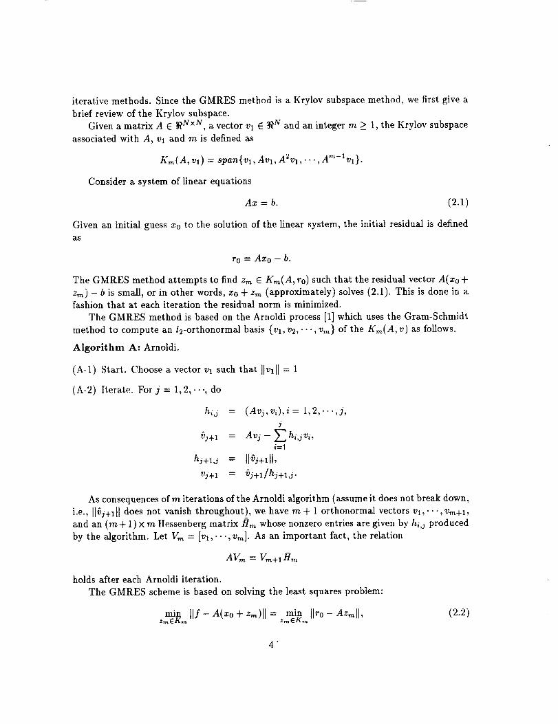
iterative methods.Sincethe GMRESmethodis a Krylov subspacemethod,wefirst giveabrief reviewof the Krylov subspace.

Givenamatrix A E _N×N, a vector Vl E _N and an integer m _> 1, the Krylov subspace

associated with A, vl and m is defined as

KIn(A, vl) = span{v1, Avl, A2vl, ... , Am-iv1}.

Consider a system of linear equations

Ax = b. (2.1)

Given an initial guess x0 to the solution of the linear system, the initial residual is defined

as

r0 = Axo - b.

The GMRES method attempts to find zm E KIn(A, to) such that the residual vector A(xo+

Zm) -- b is small, or in other words, x0 + zm (approximately) solves (2.1). This is done in afashion that at each iteration the residual norm is minimized.

The GMRES method is based on the Arnoldi process [1] which uses the Gram-Schmidt

method to compute an/2-orthonormal basis {vl, v2," ", vm} of the KIn(A, v) as follows.

Algorithm A: Arnoldi.

(A-l) Start. Choose a vector vl such that ]lVl[I = 1

(A-2) Iterate. For j = 1, 2,.. -, do

hi.j = (Avj,vi),i= 1,2,...,j,J

"Vj+I = Avj - _ hi,ivi,i=1

hj+l,j = II j+lll,

Vj+l = _)j+l/hj+l,j.

As consequences of m iterations of the Arnoldi algorithm (assume it does not break down,

i.e., II_j+ltl does not vanish throughout), we have m + 1 orthonormal vectors vl,'--, vm+l,

and an (m + 1) x m Hessenberg matrix Hm whose nonzero entries are given by hid produced

by the algorithm. Let Vm = [Vl,'" ", Vm]. As an important fact, the relation

AVm = Vm+l[Im

holds after each Arnoldi iteration.

The GMRES scheme is based on solving the least squares problem:

min I[f- A(xo + zm)l] = min llro - Azmll, (2.2)zrnEKm zmEKm

.

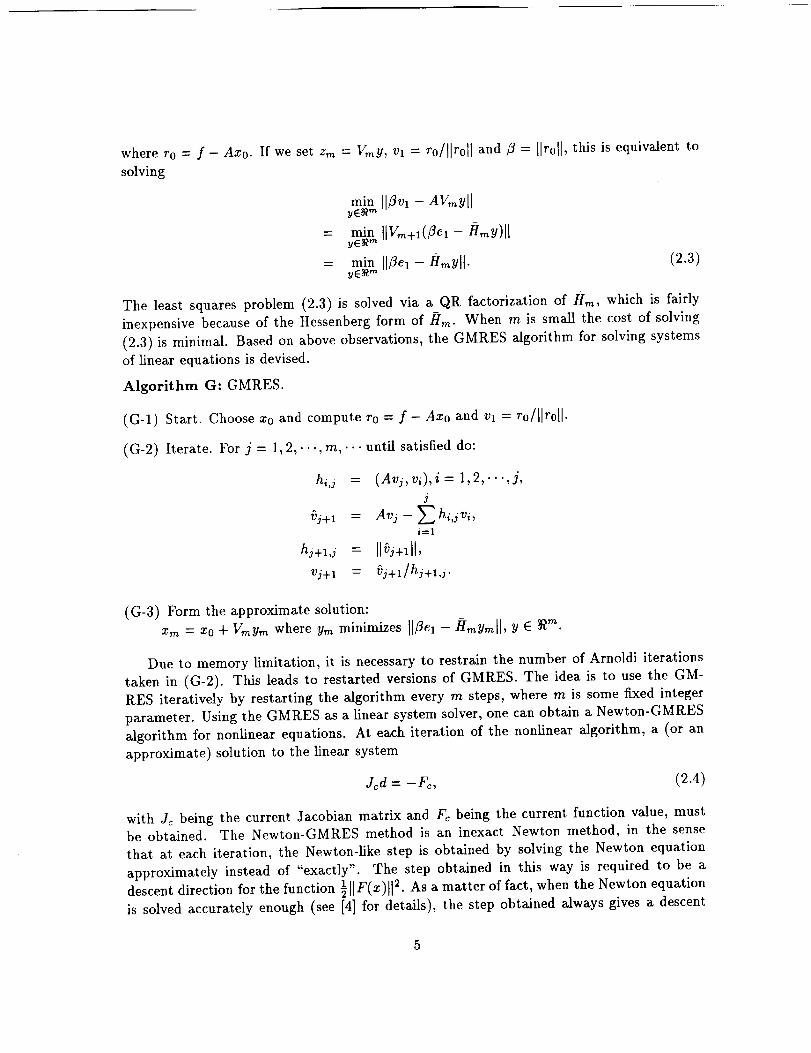
= vmy, v, = to/lit011 and J -- IIr011, this is equivalent towhere ro = f- Axo. If we set zm

solving

min II_Vl -- AVmYll

yE_ rn

= min IlUm+l(_ei -/t_Y)llyE_ rn

= min llJel - H,_YlI. (2.3)yE_ rn

The least squares problem (2.3) is solved via a QR factorization of Hm, which is fairly

inexpensive because of the Hessenberg form of Hm. When m is small the cost of solving

(2.3) is minimal. Based on above observations, the GMRES algorithm for solving systems

of linear equations is devised.

Algorithm G: GMRES.

(G-l) Start. Choose x0 and compute ro = f- Axo and Vl = ro/ilroll.

(G-2) Iterate. For j = 1,2,..-,m,... until satisfied do:

hi,j = (Avj,vi),i= 1,2,...,j,J

vj+l = Avj - Z hi,jvi'

hj+ ,j = II j+lll,Vj+I ---- Vj+l/hj+l,j.

(G-3) Form the approximate solution:Xm = XO + VmYm where ym minimizes II_el - flmYmll, Y E _ra.

Due to memory limitation, it is necessary to restrain the number of Arnoldi iterations

taken in (G-2). This leads to restarted versions of GMRES. The idea is to use the GM-

RES iteratively by restarting the algorithm every m steps, where m is some fixed integer

parameter. Using the GMRES as a linear system solver, one can obtain a Newton-GMRES

algorithm for nonlinear equations. At each iteration of the nonlinear algorithm, a (or an

approximate) solution to the linear system

Jcd = --Pc, (2.4)

with Jc being the current Jacobian matrix and Fc being the current function value, mustbe obtained. The Newton-GMRES method is an inexact Newton method, in the sense

that at each iteration, the Newton-like step is obtained by solving the Newton equation

approximately instead of "exactly". The step obtained in this way is required to be a1

descent direction for the function _ IIF(x)ll 2. As a matter of fact, when the Newton equation

is solved accurately enough (see [4] for details), the step obtained always gives a descent

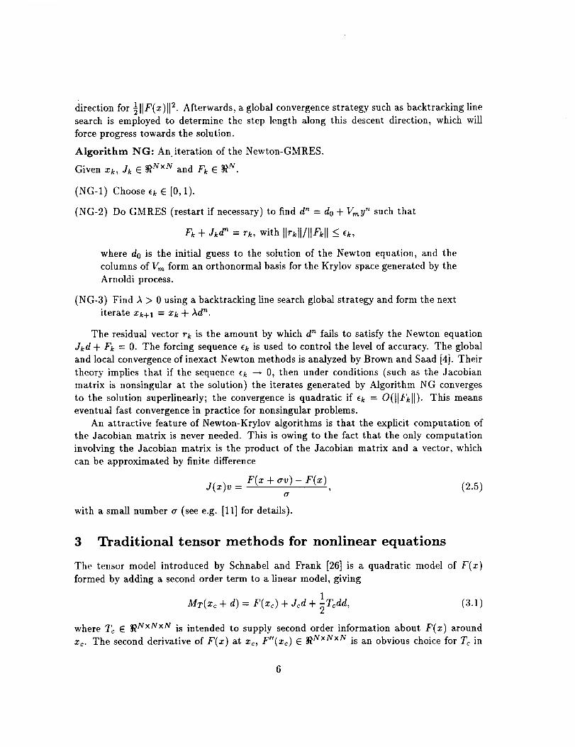
directionfor ½IIF(x)II 2. Afterwards, a global convergence strategy such as backtracking line

search is employed to determine the step length along this descent direction, which will

force progress towards the solution.

Algorithm NG: An iteration of the Newton-GMRES.

Given xk, Jk E _NxN and Fk E _N.

(NG-1) Choose 'k e [0,1).

(NG-2) Do GMRES (restart if necessary) to find d n = do + Vmy n such that

Fk + Jkd n = rk, with Ilrkll/llFkll <_ ek,

where do is the initial guess to the solution of the Newton equation, and the

columns of Vm form an orthonormal basis for the Krylov space generated by the

Arnoldi process.

(NG-3) Find )_ > 0 using a backtracking line search global strategy and form the next

iterate xk+l = xk + )_d'_.

The residual vector rk is the amount by which d'_ fails to satisfy the Newton equation

Jkd + Fk = 0. The forcing sequence _k is used to control the level of accuracy. The global

and local convergence of inexact Newton methods is analyzed by Brown and Saad [4]. Their

theory implies that if the sequence ek _ 0, then under conditions (such as the Jacobian

matrix is nonsingular at the solution) the iterates generated by Algorithm NG converges

to the solution superlinearly; the convergence is quadratic if ek = O([IFkll ). This means

eventual fast convergence in practice for nonsingular problems.

An attractive feature of Newton-Krylov algorithms is that the explicit computation of

the Jacobian matrix is never needed. This is owing to the fact that the only computation

involving the Jacobian matrix is the product of the Jacobian matrix and a vector, which

can be approximated by finite difference

J(x)v = F(x + av) - F(x), (2.5)(7

with a small number a (see e.g. [11] for details).

3 Traditional tensor methods for nonlinear equations

The tensor model introduced by Schnabel and Frank [26] is a quadratic model of F(x)

formed by adding a second order term to a linear model, giving

ir(xc + d) = F(xc) + Jcd + 1Tcdd, (3.1)

where Tc E _NxN×N is intended to supply second order information about F(x) around

xc. The second derivative of F(x) at xc, F"(Xc) E _N×N×N is an obvious choice for Tc in

6

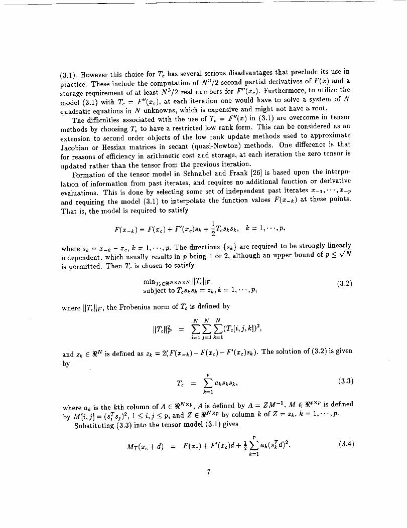
(3.1). Howeverthis choicefor Tc has several serious disadvantages that preclude its use in

practice. These include the computation of N3/2 second partial derivatives of F(x) and a

storage requirement of at least N3/2 real numbers for F"(xc). Furthermore, to utilize the

model (3.1) with Tc = F"(xc), at each iteration one would have to solve a system of N

quadratic equations in N unknowns, which is expensive and might not have a root.The difficulties associated with the use of Tc = F"(x) in (3.1) are overcome in tensor

methods by choosing Tc to have a restricted low rank form. This can be considered as an

extension to second order objects of the low rank update methods used to approximate

Jacobian or Hessian matrices in secant (quasi-Newton) methods. One difference is that

for reasons of efficiency in arithmetic cost and storage, at each iteration the zero tensor is

updated rather than the tensor from the previous iteration.Formation of the tensor model in Schnabel and Frank [26] is based upon the interpo-

lation of information from past iterates, and requires no additional function or derivative

evaluations. This is done by selecting some set of independent past iterates x-1,"-,X-p

and requiring the model (3.1) to interpolate the function values F(x_k) at these points.

That is, the model is required to satisfy

1

F(x_k) = F(x_) + F'(xc)sk + _Tcsksk, k = 1,...,p,

where sk = x-k - x_, k = 1,..-,p. The directions {sk} are required to be strongly linearly

independent, which usually results in p being 1 or 2, although an upper bound of p <

is permitted. Then Tc is chosen to satisfy

minT_e_xNxN IIT_IIFsubject to Tcsksk = zk,k = 1,...,p,

(3.2)

where IITAF, the Frobenius norm of Tc is defined by

IITdl N N N

= EE :'i=1 j=l k=l

and zk e _g is defined as zk = 2(F(x_k) - F(x_) - F'(xc)sk). The solution of (3.2) is given

by

P

T_ = _aksksk, (3.3)k=l

where ak is the kth column ofA E _Nxp, A is defined by A = ZM -1, M E _vxp is defined

by M[i,j] = (sTsj) 2, 1 < i,j < p, and Z E _gxp by column k of Z = zk, k = 1,-..,p.

Substituting (3.3) into the tensor model (3.1) gives

P

MT(Z_ + d) = F(x_) + F'(x_)d + ½ _ ak(sTd) 2. (3.4)k=l

The additional storage required by Tc is 2p N-vectors, for {ak} and {sk}. In addition, the 2p

n-vectors {x-k} and {F(z_k)} must be stored. Thus the total extra storage required for the

tensor model is at most 4N 1"5 since p < v_, which is likely to be small compared to the N 2

storage required for the Jacobian. The entire process for forming Tc requires N2p + O(Np 2)

multiplications and additions. The leading term comes from calculating the p matrix-vector

products F'(zc)Sk, k = 1,...,p; the cost of solving A = ZM -1 is O(Np2). Since p < v_,

the leading term in the cost of forming the tensor model is at most N 2"5 multiplications and

additions per iteration, but it is usually only a small multiple of N 2 arithmetic operations in

the dense case since p is usually 1 or 2. This cost also is small compared to the at least N3/3

multiplications and additions per iteration required for the dense matrix factorizations by

standard methods that use analytic or finite difference derivatives. If F'(x) is large and

sparse, the additional cost is simply p matrix-vector products, which generally is small in

comparison to the costs of a standard iteration.

Solution of the tensor model with the special form of Tc given by (3.3) also can be

performed efficiently in terms of algorithmic operations. The goal is to find a root of the

tensor model (3.4), that is,

find d E _N such thatP

MT(Xc + d) = F(z_) + F'(x_)d + 1 _ ak(sT d)2 = O. (3.5)k=l

Since (3.5) may not have a root, it is generalized to solving

min HMT(xc 4- d)]12. (3.6)d_._ N

Schnabel and Frank [26] show that the solution of (3.6) can be reduced, in O(N2p)

operations, to the least squares solution of a system of q quadratic equations in p unknowns,

plus the solution of a system of N - q linear equations and N -p unknowns. (Usually, q = p;

the exceptional case q > p arises when the system of N - p linear equations and N - p

unknowns would be singular and generally only occurs when rank(F'(z_)) < N - p.) This

reduction is carried out by performing orthogonal transformations of both the variable and

equation spaces in a way that isolates the quadratic terms into only p equations. The details

of this process are not important to this paper, because here we deal solely with models

where p = 1, in which case the tensor model can be solved much more simply and in closed

form. For these reasons we do not discuss the solution algorithm further in this paper; for

details, see [26]. The total cost of solving the tensor model is about 2N3/3 + N2p+ O(N 2)

multiplications and additions in the dense case, at most N2p < N 2'5 multiplications more

than the QR factorization of an N x N matrix. The proeess generally is numerically stable

even if F'(x_) is singular but has rank > N - p. If F'(zc) is nonsingular, the Newton step

can be obtained very cheaply as a by-product of the tensor model solution process. If F'(zc)

is large and sparse, the tensor model solution still costs very little more than the standard

Newton iteration, see [2].

In practice, computational results in [26] show the tensor method is more efficient than

an analogous standard method based upon Newton's method on both nonsingular and

8

singularproblems,with a particularlylargeadvantageonsingularproblems.In testsonastandardsetofnonsingulartestproblems,thetensormethodis almostalwaysmoreefficientthanthe standardmethodandisneversignificantlylessefficient.Theaverageimprovementby the tensormethodis 21- 23%,in termsof iterationsor functionevaluations,onal] testproblems,and 36 - 39%on the harderproblemswhereonemethodrequiresat least teniterations. The tensormethodis considerablymoreefficientthan the standardmethodon problemswith rank(F'(x.)) = N - 1; the average improvement is 40 - 43% on all

problems and 57 - 61% on the harder problems. The advantage of the tensor method overthe standard method on problems with rank(F'(x.)) = N - 2 is not as great as for the

rank(F_(x.)) = N - 1 case but is still considerable, an average of 27 - 37% improvement on

all problems and 57 - 65% on the harder problems. More recent computational experiments

in [2], including experiments on much larger problems, show similar advantages for tensor

methods.

It is shown in [13] that under mild conditions that the sequence of iterates generated

by the tensor method based upon an ideal tensor model converges locally and two-step

Q-superlinearly to the solution with Q-order 3, and that the sequence of iterates generated

by the tensor method based upon a practical tensor model converges locally and three-step3 In the same situation, it is known thatQ-superlinearly to the solution with Q-order 7.

standard methods converge linearly with constant converging to ½. Hence, tensor methods

have theoretical advantages over standard methods. The analysis in [13] also confirms that

tensor methods converge at least quadratically on problems where the Jacobian matrix at

the root is nonsingular.

4 Tensor-GMRES method for nonlinear equations

4.1 Introduction

As reviewed in the previous section, traditional tensor methods for nonlinear equations are

more successful both in theory and in practice than standard methods, notably for their fast

local convergence and their efficiency in arithmetic cost per iteration. Nevertheless, sincethese methods are based on the factorization of the Jacobian matrix (or its approximation),

they may not be attractive for many classes of large and sparse systems. Newton-Krylov

methods are very effective in many situations for nonlinear equations problems. They often

have fast local convergence as analyzed by Brown and Sa_d [4]. However, the fast local

convergence can be impaired when the Jacobian matrix is singular or ill-conditioned at the

solution. This is not uncommon in practice and accounts for a substantial amounts of the

failures of Newton-like methods. The tensor method introduced here is primarily intended

to improve upon the Newton-Krylov methods in cases where the Jacobian matrix is singular

or ill-conditioned at the solution. This is done in a fashion similar to the Newton-GMRES

method that avoids the requirement of the factorization of the Jacobian matrix by the

traditional tensor methods. As a matter of fact the Jacobian matrix is never explicitly

needed. In addition, the new method will have similar efficiency in arithmetic cost per

iteration to Newton-GMRESmethod.Thetensormodelconsideredhereusesonlyonepastiterateinformation.Therearethree

reasonsfor this. First, from thecomputationalexperiencewith tensormethodsfor nonlinearequations,the tensormethodsthat useonepast point areeasierto implementandhavemoresatisfactorycomputationalperformancein practice. Second,from theoreticalpointof view, tensormethodsbasedonsinglepastpoint arebetter understood.Third andmoreimportantly, the tensormodelbasedon usingmorepast points mayrequiresignificantlymorestoragethantheNewton-GMRESmethodsincethelatteronlyrequiresO(N) (N being

the size of the problem) memory locations and the storage of each past iterate information

requires O(N) locations as well. The situation is much different for the traditional tensor

model based methods where p, the number of past points used, can be as high as v/-N.

The major difference between the new tensor model and the traditional tensor modelis that the new tensor model has a more restricted second order term. The analysis of

tensor methods for nonlinear equations by Feng, Frank and Schnabel [13] indicates that

tensor methods will not lose fast local convergence on singular problems if the tensor term

is projected into proper subspaces. As a matter of fact, we can show that for problems

where the Jacobian matrix has rank deficiency one at the solution, if the second order

term in the tensor model is projected into the subspace spanned by the left singular vector

corresponding the smallest singular value of the Jacobian matrix, the theoretical results

given in [13] remain intact. This means that methods based on the tensor model with the

projected second order term will have fast local convergence on singular problems. This

is the theoretical foundation of our tensor-GMRES method. The idea of projected tensor

methods was first implemented in [12] for constrained optimization, where the projection is

taken place in the variable space. The difference here is that the projection occurs in the

function space.

This section is organized as follows. We first analyze two ideal tensor models that are

closely related to our new tensor-GMRES model in Subsection 4.2. The formation and

solution of the tensor-GMRES model is discussed in Subsections 4.3 and 4.4. We give a

work comparison between the tensor-GMttES method and the analogous Newton-GMRESmethod in Subsection 4.7.

Some notation is also useful to us. Throughout this section we use N to denote the

number of unknowns in the Newton equation and NZ to denote the number of nonzero

elements in the Jacobian matrix.

Let F'(xc) = UcDcV T be the singular value decomposition of F'(x) at xc, where Uc =¢ C •[u_, u_, U_v], Vc = Ivl, v2,-., V_v], and D_ = diag[a_, a_,..., a_v], with a_ > a_ > --. >°'', __ __ __

cr_, > 0 being the singular values of F'(z_) and {u_}, {v_} being the corresponding left and

right singular vectors.

Similarly, let F'(x.) = UDV T. Let v and u be the right and left singular vector of

F'(x.) corresponding to the zero singular value, when F'(z.) has rank deficiency one.

10

4.2 Analysis of tensor methods using projected second order derivatives

The sequence of iterates produced by our algorithms is invariant to translations in the

variable space. Thus no generality is lost by making the assumption that the solution

occurs at x. = 0, and this assumption is made throughtout this subsection. We also assume

that v_ and u_v are so chosen that ]lv_¢- vii = O(llxcll) and Ilu_ - ull = O(llzcll), wheneverxc is sufficiently close to x.. This assumption is valid from the theorems about continuity

of eigenvectors in Ortega [20] and Stewart [27], as long as F'(x)is continuous near z., and

has rank deficiency no greater than one at x..

Before going into the details of the analysis, we give Assumption 4.0, a group of as-

sumptions that will be invoked for the remainder of this subsection in every result involving

F(x). These assumptions basically state that near x., the second order term supplies useful

information in the null space direction of F'(x.), where F_(x.) lacks information.

Assumption 4.0 Let F : _g __. _g have two Lipschitz continuous derivatives. Let F( x. ) =

O, F'(x.) be singular with only one zero singular value, and let u and v be the left and right

singular vector of Fl( x.) corresponding to the zero singular value. Then we assume

rr"(x.)vv # 0 (4.1)

where Fl'(x.) E _NxN×N.

Assumption 4.0 is satisfied by most problems with rank(F'(x.)) = N - 1, and has

been assumed in most papers that analyze the behavior of Newton's method on singular

problems. When N = 1, Assumption 3.0 is equivalent to f"(x.) _ O.

Suppose we know the right and left singular vectors v_v and u_v corresponding to the

least singular value of F'(x_) where x_ is the current iterate and Itv_vll = Ilu_vll = 1. Then

an excellent tensor model around x_, if one is to utilize just a rank-one second order term,

is

MT._(x_ + d) = F(zc) + F'(xc)d + l (uCNuCNT)ac(vCNTd)2, (4.2)

ll C Cwhere ac = F (Xc)VNVN, because it contains the correct second order information wherethe Jacobian contains the least information, and correspondingly, where the second order

term has the greatest influence.

Based on (4.2), a simple tensor algorithm, Algorithm PT, is designed.

Algorithm PT: Projected Tensor Algorithm.

IF (4.2) has real roots THEN

d _ dR where dR solves MT_ N (xc + d) = 0

ELSE d _ dM where dM minimizes IIMT=N(X_+ d)ll[]

Since (4.2) is the basis for our new tensor-GMRES model, we give an analysis of Algo-

rithm PT.

11

Corollary 4.1 Let Assumption 4.0 hold and {xk} be the sequence of iterates produced by

Algorithm FT. There exist constants 1(1, I(: such that if ]]Xoll < K1, then the sequence {xk}

converges to x. and

IlXk+211 K llxkll

for k = 0,1,2,....

Proof. Note that I = EN=; uCu_T and Jc = EN1 (r_u_ vcT. From the orthogonality of up,

i = 1,.--,N, we have

MT_N (xc + d)

N N1 c c T cT 2

= (_-_u_u_r)(F_ + y'_a_u_v_Td+_(uUUN )a_(v N d) )i=1 i=1

N-1

= [ r d + ri=l

1 c T cT 2 cq-(a_v_T d + uCNTFc + -_U N ac(v N d) )u N. (4.3)

Note that the difference between (4.3) and (4.2) of [13] is only a second order term in the

coefficient of each u_ for i = 1,...,N - 1, which does not effect either of the proofs of

Lemmas 4.1 and 4.2 of [13]. The rest of the proof can be completed by following exactly

the proof of Theorem 4.4 of [13]. []

Now we look at an interesting tensor model that is closely related to (4.2). Let W E

_g×m with m _< N orthonormal columns. Consider the tensor model

MTw(Xc + d) = F(xc) + F'(xc)d + l (wwT)ac(v_d)2,z

(4.4)

where u_ = Wy for y _ 0, or u_ is in the span of the column vectors of W.

Corollary 4.2 Let Assumption 4.0 hold and {xk} be the sequence of iterates produced by

Algorithm PT with U_N being replaced by W. There exist constants K1, K2 such that if

Ilxoll <_ K1, then the sequence {xk} converges to x. and

II*k-+-211 K211xkll+

for k = 0,1,2,....

Proof. Since U_g = Wy, from the orthogonality of columns of W, we have

UcNucNTWWT = uCNyTWTww T = UCNyTW T = UcNucNT. (4.5)

12

By similar reasoningasstatedin the proofof Corollary4.1,and using(4.5)

MTw(Xc + d)N N

=- (_u_ucT)(Fc + _aCuCvCTd + ½(wwT)ac(v_cTd) 2)i=1 i=l

N-11 cT T c T 2 c

= [_-_ (aCv_ Td + u7TFc + -_ui (WW)ac(VN d) )ui]i----1

1 c T c T 2 c (4.6)+(a_vCNT d + uCNTFc + -_UN ac(v N d) )u N.

Again, note that the difference between (4.6) and (4.2) of [13] is only a second order termin the coefficient of each u_ for i = 1,. •., N - 1, which does not effect either of the proofs

of Lemmas 4.1 and 4.2 of [13]. The rest of the proof can be completed by following exactly

the proof of Theorem 4.4 of [13]. []

4.3 Formation of the tensor model

At the current iterate xc, assume that the Newton equation

Fc ÷ J_d n= 0 (4.7)

is solved by the GMRES method with d n = Vmym (assuming starting from zero). Let /tin

be the (m-t- 1) x m Hessenberg matrix from the Arnoldi process. An interesting fact is that

the resulting Newton step d'_ is in the span of the column vectors of Vm. The analysis of

Feng, Frank and Schnabel [13] indicates that when the Jacobian matrix has a null space ofdimension one at the solution, close to the solution, the Newton iterates fall into a funnel

around the null space. In this situation, their theory also implies that the angle between d '_

and v_, the right singular vector corresponding to the smallest singular value of the current

Jacobian matrix J_, will be arbitrarily close to zero, close to the solution. As a consequence

of d'_ = Vmym, v_v will be arbitrarily close to being in the span of the column vectors of

Vm. Consequently, u_v that is in the same direction as J_v_ will be arbitrarily close to being

in the span of the column vectors of JcV,_. Hence a good approximate to the projection

matrix WW T in (4.4) would be the projection matrix

P = (JcV,_)[(JcV,_)T(jcVm)I-I(j_V,_) T. (4.8)

The singular vectors and the exact second order derivatives used in (4.4) are normally

too expensive to obtain. We approximate them in the following manner. As in the situation

of the traditional tensor model (3.4), let sc = Xp - xc, the difference between the past iterate

xp and the current iterate xc. There are two choices for approximating v_v in (4.4), One

is using d'_/lld'_ll since the Newton step d n is likely to be along the null space close to the

solution for singular problems. Another one is using h = s¢/lls_ll since when consecutiveiterates are in the funnel around the null space near the solution, the difference between the

two consecutive iterates is also likely to be along the null space. We choose to use h because,

13

aswewill seelater, this will causeour tensormodelto interpolateapastpointin aprojectedfunctionspace.Theability ofinterpolatingpastpointsisvital for the successof traditionaltensormethodsfor nonlinearequationson both singularand nonsingularproblems.The

tl c cterm ac = F (xc)vNv N in (4.4) can be approximated by

2(r(xp)- F(xc)- J(xc)sc)

a = sTsc = F"(x_)hh + E, (4.9)

where ]]E]] = O(]lscH). Equation (4.9)is standard in tensor model formation, which requiresno extra function or Jacobian matrix evaluations.

Putting all the pieces together, we arrive at the following tensor model.

MTp(Xc + d)= Fc + Jcd + ½Pa(hTd) 2, (4.10)

where P is given by (4.8). It is easy to verify that the unprojected tensor model

MT(X_ + d) = F_ + J_d + ½a(hTd) 2 (4.11)

interpolates the function value at the past point Xp. Hence, from

fMTp(X¢ + d) = PFc + PJcd+ ½PPa(h Td) 2

1 Pa(hTd)2= PF¢ + PJcd+ -_

= P(Fc + Jcd+ ½a(hTd)2),

the interpolation property of the full tensor model (4.11) implies that the projected tensor

model (4.10) interpolates F(x) at the past Xp in the subspace resulted from the projection of

P onto the full function space. It is easy to see also that the tensor model (4.10) interpolates

F(x) at the current point in full function space. A second property of (4.10) is that when

m = N, The projector matrix P is equal to identity, which recovers the full tensor model

(4.11).

The formation of the tensor model (4.10) requires storage of two N-vectors Fp and

xp. The work of calculating a and h requires a matrix-vector multiplication costing NZ

multiplications, and the evaluation of Ilscll costing N multiplications. Since as we will see

later, we do not have to form the projection matrix P explicitly, we will count the cost of

calculations involving P to the cost of solving the tensor model, which will be addressed in

the next subsection.

4.4 Solution of the tensor model

Solving the tensor model (4.10) in the full variable space is not preferable since it would

be as expensive as solving the full tensor model. As discussed in Section 1, solving the full

tensor model could involve calling a Krylov method for linear equations twice, which could

be expensive in many situations. An alternative is to solve (4.10) in the Krylov subspace.When the Jacobian matrix lacks the first order information, close to the solution, the major

14

errorofthe currentiteratewouldlikelyresidein thespacespannedby V_v. Hence, we would

like the tensor step to be along V_v so that it would have the biggest effect on reducing the

error. Since V_v is arbitrarily close to being in the span of the columns of Vm, it is reasonable

to require that the tensor step be in the span of the columns of Vm.Therefore we would like to solve the least squares problem

min HFc + Jcz + ½Pa(hTz)21],zEKm

(4.12)

which is equivalent to solving

min NF_ + JcV,_y + ½Pa(hTVmy)211 • (4.13)yE_ m

Recall that J_Vm = Vm+l[Im. Let f-Ira = QmRm be the QR factorization of/_m. (Note

that Qm is the product of m Givens rotations; for details see [24].) From (4.8),

P = V,_+IQ,_R,_[(V,_+IQmR,_)T(v,_+IQ,_R,_)]-I(Vm+IQ,,Rm) T

= Vm+, Q_ Rm(kTRm) -' "_,_'_'TAT ,zT,m+,

Vm+l(_,_(Im O)-TT (4.14)Um+l.0 0 Q'_

Q_V_+,a,Using (4.14)and r0 = -Fc, and lettingb be the firstm components of -T T (4.13)is

equivalentto

iv,min I1- ro + Vm+,/_y + _ m+,Qm o (hTV_y)_I]yE_ m

= min IIV_+,(ll"ollel- O,_RmY - 2 0yE_ TM

= min [l_)_(_)T[Ir01lel - RmY- ½ 0 (hTVmy)2)IIyE_ rn

= min [Iw- R',,y - b(hTVmy)2[I (4.15)yE_ rn

R,_ is the first m rows of Rm. Anwhere w is the first m components of 0r_llr0ll_,and -1

interesting feature of (4.15) is that if the system of quadratics has a root, the minimum norm

of the tensor model in the Krylov space will be the absolute value of the last component

of (_T[Ir0[]el, which is the same as the residual norm of the Newton equation solved by the

GMRES algorithm. When /_1m is nonsingular, using the techniques for solving the tensor

model developed in [2], we form the j3 function

_ lhTV, _R1 ,-lb, hTV, ,2q(_) = hrV_(R1)-'_ hT"V,,,y--_ ,,,_ m) t ,,YJ= _T(R_)-I w _ fl _ ½_T(/_)-'bZ2 ' (4.16)

15

wherefl = hTVmy and h = VTh, and solve the minimization problem

min IIq(_)[I. (4.17)

Let B. be a solution to (4.17). By the theory established in [2], (4.15) is solved by

yr, = [( Rlm)T ( Rlm)]-l]_q(/_.)/_.+ (Rlm)-lw_ _( Rm )1-1 -ibm.,2

^T -1 T -1 -1 ^where a; = h [(Rm) (Rm)] h. Then the tensor step for the system of nonlinear equations

is given by

dt= Vmyt.. (4.18)

Compared to the solution of the Newton equation by the GMRES algorithm, the solution

of the tensor model requires a minimal amount of extra work. The major extra work comes

from forming d t from (4.18) and the calculation of VTh and VTa, each requiring mN

multiplications. In addition, forming the _ function requires one extra backsolve of an

m × m triangular system and two dot-products of vectors of length m, costing lm2 +

2m multiplications; forming b needs an applications of m Givens rotations, costing 4m

[(Rm) (Rm)] h requires two backsolves of an m × m triangularmultiplications; forming -1 T -1 -1 ^

system, costing m 2 multiplications, and then forming w needs a dot-product of two m-

vectors, costing m multiplications. In summary, the total extra cost of solving the tensor3 2

model is 3mN + _m + Tm.

4.5 Dealing with do # 0

Because of the memory limitation, it is necessary for the GMRES algorithm to restart. As

a result, the solution to the Newton equation obtained from the GMRES algorithm is given

by dn = do + Vmy _. In this situation, d_ is in the span of {do, V,_}, instead of in the span

of {Vm} only, as in the situation of do = 0. For reasons discussed before, we would like

the tensor step to be in the span of {do, Vm}. Consequently, we would like the projection

matrix P to be onto the subspace spanned by {JcVm, Jcdo}. One choice of such a P is

= M(MTM)-IM T

where M = J[Vm, do]. Hence we would like to solve

min IIF_+ J_d + 1pa(hTd)211. (4.19)de{do)ugm

Let d = V_y + d0r. Using r0 = -_Pc - J_do, (4.19) is equivalent to solving

yE_m,rE_ T T

= rain IIF_ + [J_V_,J_do] ryE_m,1"E_ r

16

()Y + ½Pa{hT[Vm, do] r

) ()Y + ½/3a{hT[Vm,do] Y )_11= min IIF_+ [Vm÷_H_,g] _ _ ,yE_m,fE_

(4.20)

where g = -Fc - r0. An important feature of (4.20) is that it does not involve the Jacobian

matrix Jc. We simplify (4.20) to

1^ ^T^ 2 (4.21)min []Fc+ JfJ + -_a(s y) II,_E_m+a

Y) h = Pa and _ = [Vm,do]Th. We discuss how to form

\

where J -=- [Vm+l Hm, g], _) = _. ,/

and solve (4.21) efficiently. The solution of this type of nonlinear least squares problem is

studied by Schnabel and Bouaricha in [25]. Their theory shows that when J has full rank

the solution of (4.21) is given by

1 ^ 2fl. = ( jT j)-I _ q(_.)/w - (JT,])-a jT (Fc + _a_. ), (4.22)

where q(/_) and w are defined by

1AT AT ^ --1 AT^ 2q(_) = ff(,]Tj)-XjTFc +_ + _s (J J) J a_ , (4.23)

w = $(jTj)-a$, (4.24)

and the value of/3. is determined from

rain IIq(_l/v_ll 2 + Iln(_)ll 2, (4.25)

where IIn(_)ll2 = II(Fc- PF_)+ ½(a- Pa)_ll _.In our situation, since /3 is a projector matrix and

a-/35 =/3a-/3/3a = Pa-/3a = O,

n(_) is a constant function. Hence the minimization problem (4.25) is equivalent to

min IIqO)ll. (4.26)

To obtain _). the critical computational work comes from the factorization of iT j,since when this factorization is available, all the computations involving (,IT j)-I can be

achieved through backsolves. For this reason, we discuss the factorization of jTj. Recall

that J = [Vm+lftm,g] and Hm = QmRm. Hence we have

gTj ____ [Ym+l_-Im,g]T[ym+l[Im,g]

17

-v • )H m Vlm+lg

= gTVm+l Y-Ira gTg

//mV_+lg= gTVm+l fI m gTg

= W T "_ 0 7

-1 -T Twhere R m is the first m rows of/_m, w = QmV_m+lg, and 7 = x/gTg- wTw. The factor-

ization is possible since jTj is always at least positive semidefinite. After Y. is obtained,

(4.19) is solved by

dr= [Vm,do]_..

However, the calculation of expressions involving (jT])-I is impossible if 7 = 0. We

discuss how to overcome this difficulty. Since j = [Vm+lHm,g] and Vm+l[tm has full rank,

g has to be in the span of {Vm+l[Im}, which implies that Jcdo = g is in the span of

JcVm = Vm+l[Im. When Jc has full rank, this implies that do is in the span of {Vm}, which

in turn implies that d n = do + Vmy n is in the span of Vmy '_. In this situation, based on

previous discussions, we actually would like to solve the tensor model (4.10) in the Krylov

subspace Vm only, i.e.

min life + Jc(do+ z)+ ½Pa(hT(do+ z))2[[,zEKm

(4.27)

where P is given by (4.8), which is equivalent to solving

min IIF= + J¢do + J¢Vmy + ½Pa(hT(do + Vmy)) ll.yE_ rn

(4.28)

Using J_Vm = Vm+l[-I,_, fire = QmRm, ro = -_Pc - J_do and (4.14), and letting b be the

first m components of -T TQmV_+la , (4.28)is equivalent to

1 - (b)(hT(do+Vmy))2[[min [[ - ro + Vm+l[Imy + -_Vm+lOm 0RE_ TM

= uemin_cm[[Um-Fi([[r0[[el-OmRmy - -_Oml- ( on )(hT(do._ - Wmy))2)[[

= min IIQm(Qr.,ll,-ollel- R,.,,y- ½ 0yG_ m

= min Ilw- [_y-b(hT(do+ Vmy))2[[yE_ rn

(4.29)

where w is the first m components of OTIIr011eland /_1 is the first m rows of/_m. Again

using the techniques for solving the tensor model of nonlinear least squares developed in

18

[2], we form the f_ function

q(_) hTVm([_lm)-I hTVmy 1 T -1 )-1= w - - -_h Vm(Rm b(hT(do + VmY)) 2

- Rm)= hT(R1)-lw + hTdo-/3 I"T_h (-1 --1 2 (4.30)

where/3 hZ(do + Vmy) and h T= = V,_ h, and solve the minimization problem

min IIq(_)ll.BE_

(4.31)

Let/_. be a solution to (4.31). By the theory established in [2], (4.29) is solved by

-1 --1 2yt, = [([_lm)r([_)]--lhq(/3,)/W + (Rlm)-' w - ½(Rm) b/_,.

Then the tensor step for the system of nonlinear equations is given by

= V, td t do+ my.. (4.32)

We examine the cost of solving the tensor model when do _ 0. Since the situation of

7 = 0 is less expensive to deal with, we will concentrate on the situation of 7 _ 0. Compared

to the solution of the Newton equation by the GMRES algorithm in a similar situation, the

solution of the tensor model requires a minimal amount of extra work. The major extra

work comes from forming d t, g, JTh and jTFc, each requiring (m + 1)N multiplications

(note that jT h = jT pa = jT a from the definition of P). Since VT+lg = vT+I(-Fc - ro) =

-vT+IFc -[Ir0llel, given vT+IFc, cost of vT+lg is only a single subtraction. Hence theQmV_+lg ' gTg and wTw,cost of factorization of iT j, which involves the calculation of -T T

is N + 5m multiplications. The operation count is accumulated from an application of

m Givens rotations costing 4m multiplications, a dot-product of 2 N-vectors costing N

multiplications and a dot-product of 2 m-vectors costing m multiplications. Given _, iT5

and jTFc, the major cost of forming q(/_) and w defined in (4.23) and (4.24) respectively,comes from the calculation of ,_T(jTj)-I. Using the available factorization of iT j, this can

be done by two backsolves of (m + 1) × (m + 1) triangular systems, which costs (m + 1) 2

multiplications. After _T(jWff)-I is obtained, the cost of forming q(f_) and w is three dot-

products of two m-vectors costing 3m multiplications totally. The cost of obtaining _). using

(4.22) needs two extra backsolves of (m+ 1) × (m+ 1) triangular systems, which costs (m + 1)2

multiplications, given _T(_Tj)-I, ffT_ and JTFc. In summary, the total extra work required

by solving the tensor model when the d _ 0 is at most (4(m + 1) + 1)N + 2(m + 1) 2 + 8m

multiplications.

4.6 Preconditioning and matrix free implementation

The success of the GMRES method on a system of linear equations usually depends on

a good preconditioner. The formation and solution of the tensor model is consistent with

preconditioning. When a preconditioner M is used in solving the Newton equation by the

GMRES algorithm, it turned out that the only thing we need to do in the tensor step

19

calculationis to replacea by M-la, and Fc by M-1Fc (in case when do _ 0). The rest of

the solution procedure is unchanged.

Compared to the Newton-GMRES method, the only extra computation involving the

Jacobian matrix in the tensor-GMRES method is the computation of Js in the formation

of the tensor term. In a Jacobian free implementation, this matrix-vector product can be

approximated by the finite difference formula specified by (2.5). Hence the tensor-GMRES

scheme is consistent with matrix free implementation.

4.7 Work comparison

If m steps of GMRES is required for solving the Newton equation, the computational cost

of the Newton-GMRES iteration is m(m ÷ 2)N + mNZ multiplications, and the storage

requirement is (m + 2)N [24]. The extra storage required by the tensor-GMRES method is 2

N-vectors. As analyzed at the end of Subsection 4.3, the extra computational cost of forming

the tensor model is N ÷ NZ. As analyzed in Subsection 4.5, in the most expensive case the

extra computational cost of solving the tensor model is (4(m + 1)+ 1)N + 2(m + 1)2+ 8m

multiplications. Hence the combined extra computational cost of formation and solution

of the tensor model in each tensor iteration, compared to an iteration of Newton-GMRES

algorithm, is at most (4(m + 1) + 2)N + 2(m + 1) 2 + 8m + NZ multiplications. If we

count the operations in flops (counting both multiplications and additions), the total extra

computational operations are at about twice as many. Compared to m(m + 2)N + mNZ,

the cost of solving the Newton equation using the GMRES method, this extra cost is not

significant if m is relatively large.

Because of the memory limitation, it is likely that m is not too large. Hence it is

necessary to restart the GMRES algorithm. However, we should point out that the tensor

model is not formed until the Newton equation is approximately solved by the GMRES

algorithm, or in other words, until the Krylov space that contains the solution to the

Newton equation is found. We form the tensor model only using the Krylov subspace

generated in the last restarted GMRES algorithm. The tensor model has nothing to do

with the intermediate Krylov spaces generated by the GMRES algorithm resulted from

restarts before the final restart. Therefore compared to the total cost of the Newton-

GMRES with restarts, the extra cost of formation and solution of the tensor model is likely

to be minimal for a large portion of nonlinear problems, particularly hard problems that

need many restarts of the GMRES algorithm.

5 Implementation and testing

In the previous section we presented the main new features of our tensor-GMRES method

for nonlinear equations, namely, how we form the quadratic model of the nonlinear function,

and how we solve this model efficiently. In this section first we give the complete algorithm

we have implemented to test these ideas and clarify various aspects of this algorithm and its

computer implementation. Then, we present some results of testing the method on several

2O

problems.This sectionis organizedasfollows.Subsection5.1givesacompletetensor-GMRESal-

gorithmfor systemsof nonlinearequationsanddiscussestheimplementationof eachstepindetails.In Subsections5.2-5.4wewill showcomparativetest resultsfor thetensor-GMRESalgorithm,Algorithm TG, givenin Subsection5.1versusthe Newton-GMRESalgorithm,AlgorithmNG,givenin Section2 with the sameimplementation.Threedistinct testprob-lems.,i.e., a Bradu problem,the BroydenTridiagonalproblemand the one-dimensionalEulerequationsproblem,andseveralof their variants,wereusedin the testing. Thetestson theBraduproblem,the BroydenTridiagonalproblemandtheir variantswereperformedon a Sun SuperWorkstation11+/50 at RIACS using MATLAB. The test on the one-dimensionalEulerequationsproblemwasperformedona CrayY-MP at NASfacilityusingFortran90. Testresultsaresummarizedand discussedin Subsection5.5.

5.1 A complete algorithm

This subsection presents Algorithm TG, the full algorithm of the tensor-GMRES method

and discusses implementation issues of this algorithm in details.

Algorithm TG. An iteration of the tensor-GMRES method.

Given xk E _N, xk-1, Jk E _N×N, Fk E _N and Fk-1 E _N.

(TG-1) Decide whether to stop. If not:

(TG-2) .Set s = xk-1 - xk, a = 2(Fk-1 - Fk - Jks)/(s Ts) and h = s/lls[I. Choose

• [0,1).

(TG-3) Do GMRES (restart if necessary) to find d n = do + V,,_y '_ such that

IIFk + Jkd'_l[ < Ek,

where do is the starting point of the last restarted GMRES procedure, and the

columns of Vm form an orthonormal basis for the Krylov space generated by the

corresponding Arnoldi process. In addition, let /Ira be the Hessenberg matrix

generated from the Arnoldi process, and Hm = QmRm be its QR-factorization.Let -1Rm be the first m rows of/_m-

(TG-4) If do = 0 or do • {Vm} then

Solve

min IIFk + Jkdo + JkV,,,y + ½ft{hT(do + Vmy)}211, (5.1)yE_ rn

where a = (JkV,_){(JkV,_)T(JkVm)}-l(JkVm) Ta, by first solving

h 1 (Rm) w + hTdo - 13- -_'°1 _*_,_min Ilql(/_)(= "T -1 -1 1i,T[_I )-lb_2)ll,

21

to obtainasolution3., where w is the first m components of QT [[Fk +

Jkdo[[el, b is the first m components of T TQ,_V_+la , and ]h = V Th.

Then the solution to (5.1) is given by

yr. = -1 T -1 -1[(Rm) (Rm)] ]hql(f_.)/w + (k_)-lw _ _(Rm )1-1 -1b/_.,2

where w = ]_T[(/_lm)T(- 1Rm)]-1^hl.

Form the tensor step d t = do + V,nyt..

Otherwise (do # 0 and do _ {Vm}),

Solve

1 ^ ^T^2min IlFc+ J_) + _a(h 2 y) 11, (5.2)

_E_m+ 1

where J = [Vm+lHm, u],

fi = (J[Vm, do]){ ( J[V,,, do])T (J[Vm, do]) }-l( J[Vm, do])T aand h2 = [Vm, do]Th. This is done by first solving

min 11q2(/3)(= hT(jTJ)-ljTFc + _ + ½hT(jTj)-ljTh_2)[[

with solution j3,. Then the solution to (5.2) is given by

1^ 2fl. = ( jT j)-l h2q2(/3,)/_ - (JT J)-l jT ( Fc + ]a_,),

where w = h_jTj)-lh 2.

Form the tensor step dt = [Vm, d0]t)..

(TG-5) Choose a new step d from d'_ and d _.

(TG-6) Find A > 0 using a backtracking line search global strategy and form the next

iterate xk+ 1 = x k .-_ Ad.

Several tests are performed to determine whether to stop the algorithm in Step (TG-1).

These stopping criteria are described by Dennis and Schnabel in Chapter 7 of [11]. For the

sake of simplicity, we only use simplified versions of their criteria. The first test determines

whether xk solves the problem (1.1). This is accomplished by using IIF(xk)][ <_ FTOL, where

a typical value of FTOL is around 10 -s, but the users can specify their own values for this

tolerance. In our tests this value was set to 10-12 since we wanted to push the algorithms

to their limits. The second test determines whether the algorithm has converged or stalled

at xk. It is done by measuring the relative change in the iterates from one step to the next.

We use ]lxk - xk_lll/lIxk_lll <_ STPTOL, where a typical STPTOL is around 10 -s in our

implementation. Finally, we test if a maximum number of iterations is exceeded. Currentlythis value is 150.

22

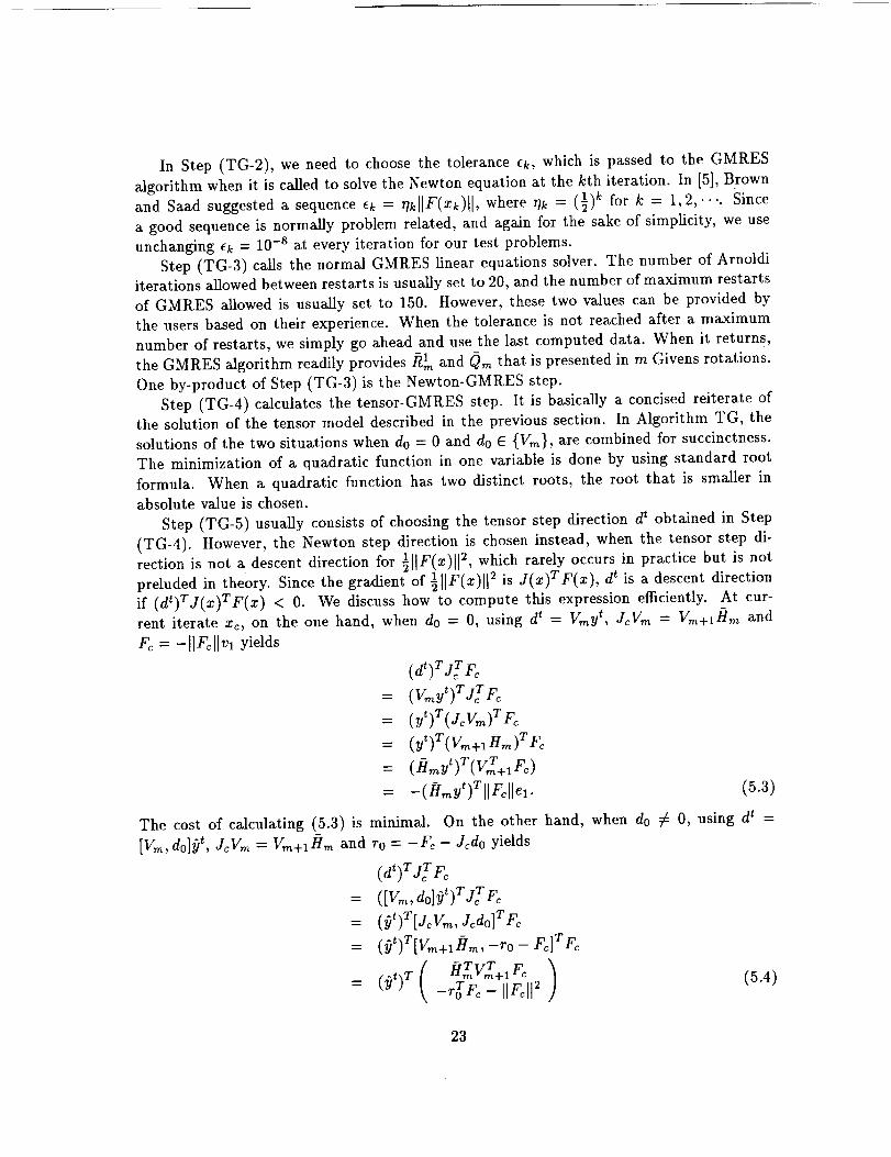
In Step(TG-2), weneedto choosethe toleranceek, which is passed to the GMRES

algorithm when it is called to solve the Newton equation at the kth iteration. In [5], Brown

and Saad suggested a sequence ek = 7?kllF(xk)[I, where rlk = (½)k for k = 1,2,.... Since

a good sequence is normally problem related, and again for the sake of simplicity, we use

unchanging ek = 10 -8 at every iteration for our test problems.

Step (TG-3) calls the normal GMRES linear equations solver. The number of Arnoldiiterations allowed between restarts is usually set to 20, and the number of maximum restarts

of GMRES allowed is usually set to 150. However, these two values can be provided by

the users based on their experience. When the tolerance is not reached after a maximum

number of restarts, we simply go ahead and use the last computed data. When it return s ,

Rm and Q,_ that is presented in m Givens rotations.the GMRES algorithm readily provides -1

One by-product of Step (TG-3) is the Newton-GMRES step.

Step (TG-4) calculates the tensor-GMRES step. It is basically a concised reiterate ofthe solution of the tensor model described in the previous section. In Algorithm TG, the

solutions of the two situations when do = 0 and do E {Vm}, are combined for succinctness.

The minimization of a quadratic function in one variable is done by using standard root

formula. When a quadratic function has two distinct roots, the root that is smaller in

absolute value is chosen.

Step (TG-5) usually consists of choosing the tensor step direction d t obtained in Step

(TG-4). However, the Newton step direction is chosen instead, when the tensor step di-

rection is not a descent direction for ½[[F(x)[[ 2, which rarely occurs in practice but is not1 F x) 2 j(x)TF(x), d tpreluded in theory. Since the gradient of _[[ ( [[ is is a descent direction

if (dt)TJ(x)TF(x) < 0. We discuss how to compute this expression efficiently. At cur-rent iterate xc, on the one hand, when do = 0, using d_ = Vmy t, JcVm = Vm+lHm and

Fc = -[[Fc[Ivl yields

(d*)T jT Fc

= (Ymyt)rjTF¢

= (y*)T(J_vm)TF_

= (yt)T(vm+I[-I,_)TF_

= ( my')r(VZ+lFc)= _([Irnyt)T][Fc[]el. (5.3)

The cost of calculating (5.3) is minimal. On the other hand, when do _ 0, using d t =

[Vm, d0]_ t, JcVm = Vm+l[Im and ro = -Fc - Jcdo yields

(dt)T jT F_

= ([Vm, do]flt)TjTF_

= (_)t)T[jcVm, J¢do]TF_

= (_)t)T[vm+,Hm,-to - F_]TFc

-T T )Hm V_+ I F¢

-%rF _ IIF=II2(5.4)

23

The major work in (5.4) is the calculationof VTm+IFc. However, since this calculation is

already done in the solution of the tensor step, no extra cost is necessary.

Finally, in Step (TG-6), we use a standard quadratic backtracking line search algorithm

which is given below as Algorithm QB. The merit function I[[F(x)H 2 is used for measuring

the progress towards the solution.

Algorithm QB Standard quadratic backtracking line search algorithm.

Given a current point xc, a search direction d, the directional derivative _, and a = 10 -4.

(QB-1) Set fc = @llF(xc)[I2 and x+ = xc + d.

(QB-2) Set f+ = ½11F(_+)II_ and A = t.

(QB-3) While f+ > fc + a. A-_ do

A_:mp= -_/(2[/+ - fc - _]);

A = max{Atemp, A/10};

x+ = xc + Ad;

/+ = ½1JF(_+)115

EndWhile

When d '_ is chosen in Step (TG-5), the directional derivative is given by (d'_)TjTFc. Its

calculation can be accomplished in a fashion similar to when d _ is chosen. When do = 0,

we can simply replace yt in (5.3) by yn and calculate -(B'my'_)[IFd[el. When do _ 0

(dn)TjTFc

= (do+ Y_y=)rJfr_= (Jcd0 + J_Vmy'_)TFc

= (-F_ - ro d- Vm+I[-I,_Y'_)TFcnT-T T

= -IIF_II_ - rTF_ + (y) Hm(V,_+IFc),

which is easy to calculate given vT+I F_.

5.2 Test results for a Bradu problem and its variants

As a first test problem we choose to solve the nonlinear partial differential equation

-Au=Ae _ in fl, u=0 on F, (5.5)

where A = V2 = _,_=12 02/cOx_ is the Laplace operator, fl = (0,1)× (0,1) and F is the

boundary of ft. This version of Bradu problem is chosen from a set of nonlinear model

problems collected by Mot6 [18].

24

0

i

-5

i-1C

-1!i i i i

1 2 3 4 5ttermlors

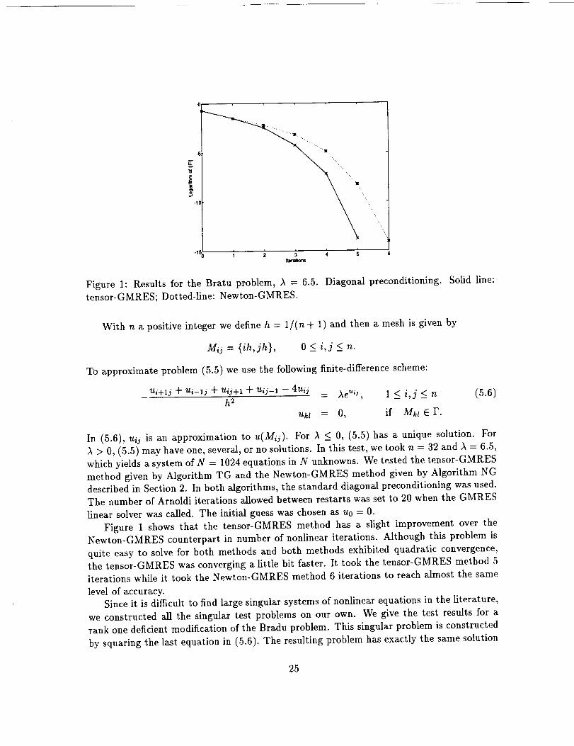
Figure 1: Results for the Bratu problem, _ = 6.5. Diagonal preconditioning. Solid line:

tensor-GMRES; Dotted-line: Newton-GMRES.

With n a positive integer we define h = 1/(n + 1) and then a mesh is given by

M_j = {ih,jh}, 0 <_ i,j <_ n.

To approximate problem (5.5) we use the following finite-difference scheme:

Ui+lj "_ Ui-lj q- Uij%l "_-Uij-1 -- 4uij = Ae,,,j ' 1 _ i,j <_ n (5.6)h 2

uk_ = O, if Mkl E F.

In (5.6), uij is an approximation to u(Mij). For A _< 0, (5.5) has a unique solution. For

> 0, (5.5) may have one, several, or no solutions. In this test, we took n = 32 and _ = 6.5,

which yields a system of N = 1024 equations in N unknowns. We tested the tensor-GMRES

method given by Algorithm TG and the Newton-GMRES method given by Algorithm NGdescribed in Section 2. In both algorithms, the standard diagonal preconditioning was used.

The number of Arnoldi iterations allowed between restarts was set to 20 when the GMRES

linear solver was called. The initial guess was chosen as u0 = 0.

Figure 1 shows that the tensor-GMRES method has a slight improvement over theNewton-GMRES counterpart in number of nonlinear iterations. Although this problem is

quite easy to solve for both methods and both methods exhibited quadratic convergence,the tensor-GMRES was converging a little bit faster. It took the tensor-GMRES method 5

iterations while it took the Newton-GMRES method 6 iterations to reach almost the same

level of accuracy.Since it is difficult to find large singular systems of nonlinear equations in the literature,

we constructed all the singular test problems on our own. We give the test results for a

rank one deficient modification of the Bradu problem. This singular problem is constructed

by squaring the last equation in (5.6). The resulting problem has exactly the same solution

25

-10

-12

110 1'5 210 25

Ittrdn

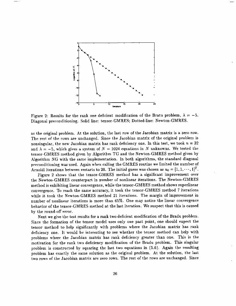
Figure 2: Results for the rank one deficient modification of the Bratu problem, A = -5.

Diagonal preconditioning. Solid line: tensor-GMRES; Dotted-line: Newton-GMRES.

as the original problem. At the solution, the last row of the Jacobian matrix is a zero row.

The rest of the rows are unchanged. Since the Jacobian matrix of the original problem is

nonsingular, the new Jacobian matrix has rank deficiency one. In this test, we took n = 32

and A = -5, which gives a system of N = 1024 equations in N unknowns. We tested the

tensor-GMRES method given by Algorithm TG and the Newton-GMRES method given by

Algorithm NG with the same implementation. In both algorithms, the standard diagonal

preconditioning was used. Again when calling the GMRES routine we limited the number ofArnoldi iterations between restarts to 20. The initial guess was chosen as u0 = [1, 1,..-, 1]T.

Figure 2 shows that the tensor-GMRES method has a significant improvement over

the Newton-GMRES counterpart in number of nonlinear iterations. The Newton-GMRES

method is exhibiting linear convergence, while the tensor-GMRES method shows superlinear

convergence. To reach the same accuracy, it took the tensor-GMRES method 7 iterations

while it took the Newton-GMRES method 21 iterations. The margin of improvement in

number of nonlinear iterations is more than 65%. One may notice the linear convergence

behavior of the tensor-GMRES method at the last iteration. We suspect that this is caused

by the round-off error.

Next we give the test results for a rank two deficient modification of the Bradu problem.Since the formation of the tensor model uses only one past point, one should expect the

tensor method to help significantly with problems where the Jacobian matrix has rank

deficiency one. It would be interesting to see whether the tensor method can help with

problems where the Jacobian matrix has rank deficiency greater than one. This is the

motivation for the rank two deficiency modification of the Bradu problem. This singular

problem is constructed by squaring the last two equations in (5.6). Again the resulting

problem has exactly the same solution as the original problem. At the solution, the lasttwo rows of the Jacobian matrix are zero rows. The rest of the rows are unchanged. Since

26

2

-2 ""A"'m 'u

6 W, M"m',

-12 "'!

.14 / L n : :0 5 10 15 20

Ileratlons

z_

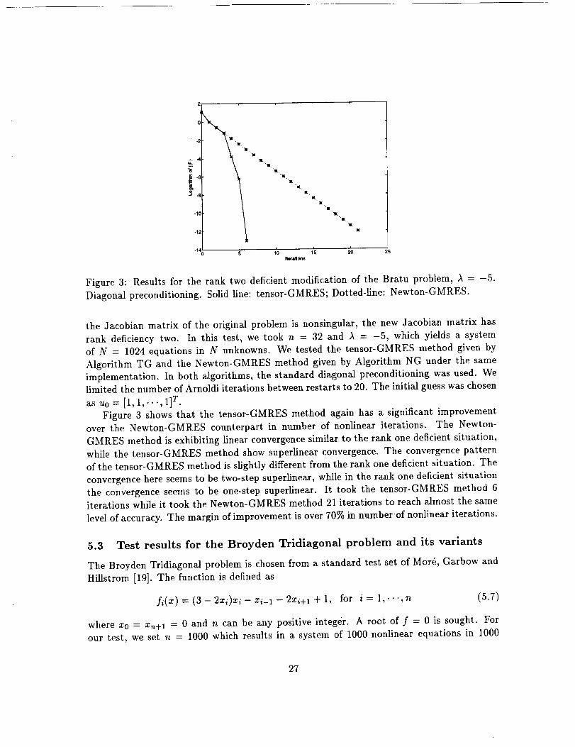
Figure 3: Results for the rank two deficient modification of the Bratu problem, A = -5.

Diagonal preconditioning. Solid line: tensor-GMRES; Dotted-line: Newton-GMRES.

the Jacobian matrix of the original problem is nonsingular, the new Jacobian matrix has

rank deficiency two. In this test, we took n = 32 and A = -5, which yields a system

of N = 1024 equations in N unknowns. We tested the tensor-GMRES method given by

Algorithm TG and the Newton-GMRES method given by Algorithm NG under the same

implementation. In both algorithms, the standard diagonal preconditioning was used. Welimited the number of Arnoldi iterations between restarts to 20. The initial guess was chosen

as u0 = [1,1,..-,1] T.

Figure 3 shows that the tensor-GMRES method again has a significant improvementover the Newton-GMRES counterpart in number of nonlinear iterations. The Newton-

GMRES method is exhibiting linear convergence similar to the rank one deficient situation,

while the tensor-GMRES method show superlinear convergence. The convergence pattern

of the tensor-GMRES method is slightly different from the rank one deficient situation. The

convergence here seems to be two-step superlinear, while in the rank one deficient situation

the convergence seems to be one-step superlinear. It took the tensor-GMRES method 6

iterations while it took the Newton-GMRES method 21 iterations to reach almost the same

level of accuracy. The margin of improvement is over 70% in numberof nonlinear iterations.

5.3 Test results for the Broyden Tridiagonal problem and its variants

The Broyden Tridiagonal problem is chosen from a standard test set of Mor6, Garbow and

Hillstrom [19]. The function is defined as

fi(x)=(3-2xi)xi-xi-l-2xi+lW1, for i= 1,...,n (5.7)

where x0 = xn+l = 0 and n can be any positive integer. A root of f = 0 is sought. For

our test, we set n = 1000 which results in a system of 1000 nonlinear equations in 1000

27

unknowns.TheJacobianmatrix hasfull rank at the solution.Threetestswereperformedon this problem.The standardstartingpoint is x0 = [-1,-1,..-,-1]. When calling theGMRES routine we limited the number of Arnoldi iterations between restarts to 20.

u.

E

-1{

'.,.

01s ; l!s _ 21s _ 31s ; ,isItwdom

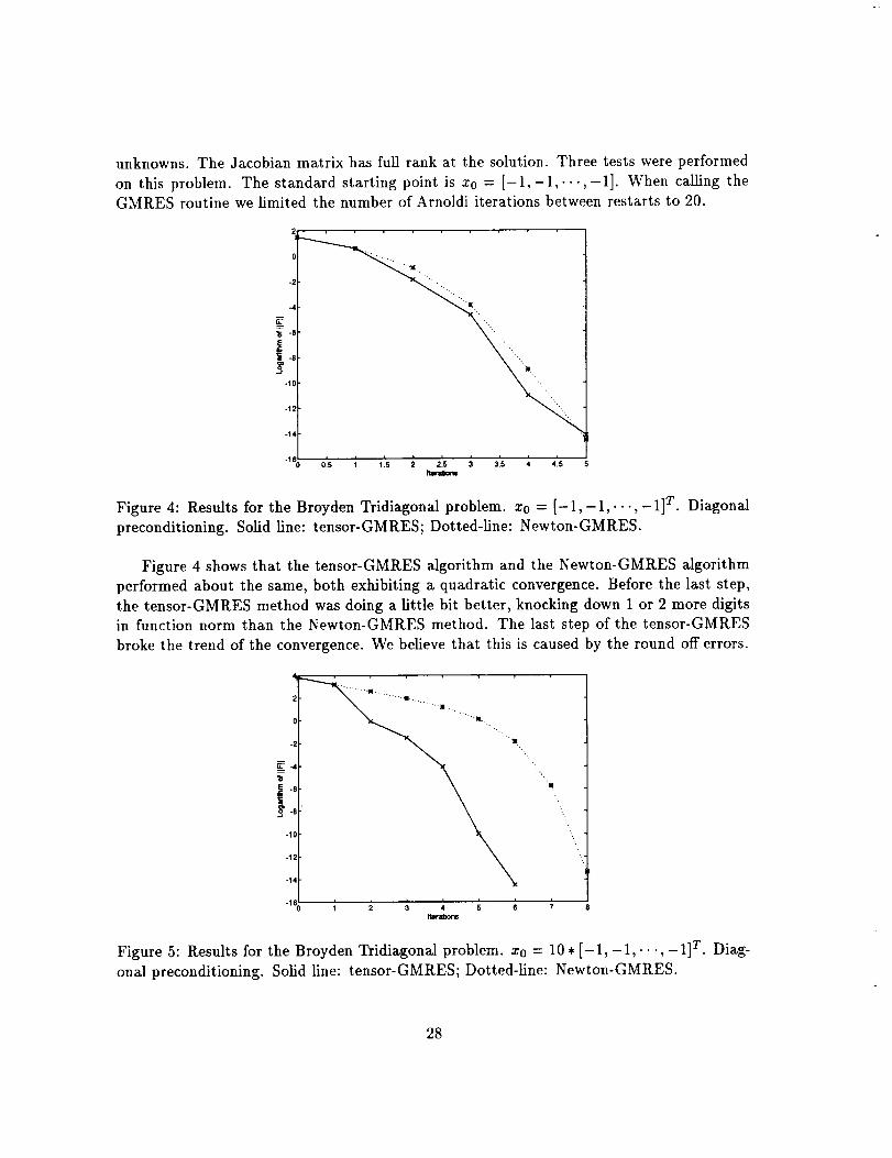
Figure 4: Results for the Broyden Tridiagonal problem. Zo = [-1,-1,..-,-1] T. Diagonal

preconditioning. Solid line: tensor-GMRES; Dotted-line: Newton-GMRES.

Figure 4 shows that the tensor-GMRES algorithm and the Newton-GMRES algorithm

performed about the same, both exhibiting a quadratic convergence. Before the last step,

the tensor-GMRES method was doing a little bit better, knocking down 1 or 2 more digitsin function norm than the Newton-GMRES method. The last step of the tensor-GMRES

broke the trend of the convergence. We believe that this is caused by the round off errors.

0 """K

-2

_4

-10 ".

-12

-14

i i i i i.1,; 1 i 3 4 _ .i_'Uarw

Figure 5: Results for the Broyden Tridiagonal problem, x0 = 10. [-1,-1,...,- 1]T. Diag-

onal preconditioning. Solid line: tensor-GMRES; Dotted-line: Newton-GMRES.

28

• Ill ...... t11¸¸ -.,J k "-m..

"m

J

2 4 6 8_rallons

It

"]

lJO 12

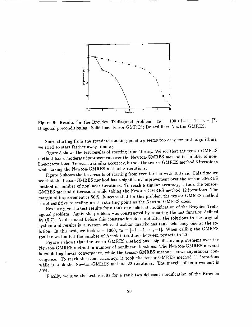
Figure 6: Results for the Broyden TridiagonaJ problem, x0 = 100 * [-1,-1,...,-1] T.

Diagonal preconditioning. Solid line: tensor-GMRES; Dotted-line: Newton-GMRES.

Since starting from the standard starting point x0 seems too easy for both algorithms,

we tried to start farther away from x0.

Figure 5 shows the test results of starting from 10 • x0. We see that the tensor-GMRESmethod has a moderate improvement over the Newton-GMRES method in number of non-

linear iterations. To reach a similar accuracy, it took the tensor-GMRES method 6 iterations

while taking the Newton-GMRES method 8 iterations.

Figure 6 shows the test results of starting from even farther with 100 * x0. This time wesee that the tensor-GMRES method has a significant improvement over the tensor-GMRES

method in number of nonlinear iterations. To reach a similar accuracy, it took the tensor-

GMRES method 6 iterations while taking the Newton-GMRES method 12 iterations. The

margin of improvement is 50%. It seems that for this problem the tensor-GMRES method

is not sensitive to scaling up the starting point as the Newton-GMRES does.

Next we give the test results for a rank one deficient modification of the Broyden Tridi-

agonal problem. Again the problem was constructed by squaring the last function defined

by (5.7). As discussed before this construction does not alter the solutions to the original

system and results in a system whose Jacobian matrix has rank deficiency one at the so-lution. In this test, we took n = 1000, x0 = [-1,-1,...,-1]. When calling the GMRES

routine we limited the number of Arnoldi iterations between restarts to 20.

Figure 7 shows that the tensor-GMRES method has a significant improvement over the

Newton-GMRES method in number of nonlinear iterations. The Newton-GMRES method

is exhibiting linear convergence, while the tensor-GMRES method shows snperlinear con-

vergence. To reach the same accuracy, it took the tensor-GMRES method 11 iterationswhile it took the Newton-GMRES method 22 iterations. The margin of improvement is

50%.

Finally, we give the test results for a rank two deficient modification of the Broyden

29

Tridiagonalproblem. The problemwasconstructedby squaringthe last two functionsdefinedby (5.7). As discussedbeforethis constructiondoesnot alter the solutionsto theoriginalsystemandresultsin a systemwhoseJacobianmatrix hasrank deficiencytwo atthe solution. In this test, we took n = 1000, x0 = [-1,-1,...,-1]. When calling the

GMRES routine we limited the number of Arnoldi iterations between restarts to 20.

!-1;

44

-le

"'it

li ..ll t

ill"ll

II it

"ill, it.

,_ ,'olllllons

"ill."ill

it"it.

'ill

I_S 20 2S

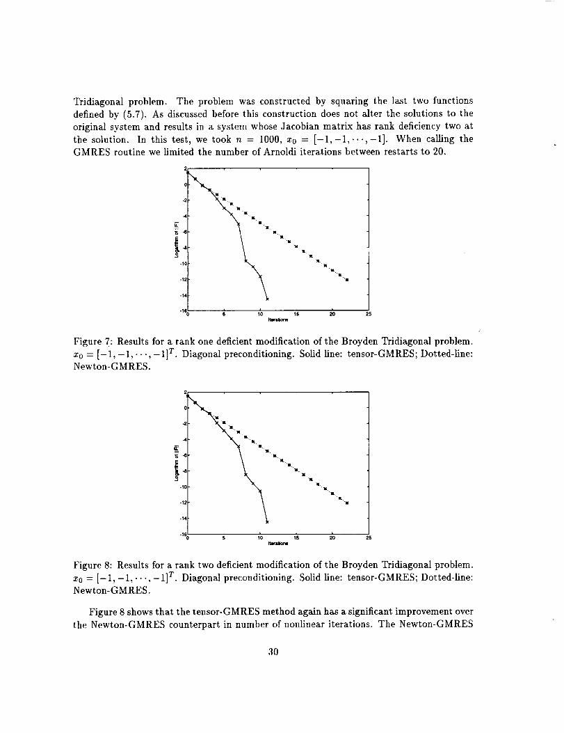
Figure 7: Results for a rank one deficient modification of the Broyden Tridiagonal problem.

x0 = [-1, -1,..., -1] T. Diagonal preconditioning. Solid line: tensor-GMRES; Dotted-line:Newton-GMRES.

2 , ,

0 "m

-2 +'it,"ll

4_it "lit

_ "'IE

_ 4 it"it K

..-12_-11

k-1E S 110

Iteraliorw

it..ilL.

'll,is

'li

"it,"m

1IF; 20 2G

Figure 8: Results for a rank two deficient modification of the Broyden Tridiagonai problem.

x0 -- [- 1, - 1,..., - 1]T. Diagonal preconditioning. Solid line: tensor-GMRES; Dotted-line:Newton-GMRES.

Figure 8 shows that the tensor-GMRES method again has a significant improvement over

the Newton-GMRES counterpart in number of nonlinear iterations. The Newton-GMRES

3O

methodis exhibiting linear convergencesimilar to the rank onedeficientsituation, whilethe tensor-GMRESmethodshowsnperlinearconvergence.The convergencepattern of thetensor-GMRESmethodagainis slightlydifferentfromtherankonedeficientsituation. Theconvergencehereseemsto betwo-stepsuperlinear,whilein therankonedeficientsituationthe convergenceseemsto beone-stepsuperlinear.It took the tensor-GMRESmethod 11iterationswhileit took theNewton-GMRESmethod22iterationsto reachalmostthesamelevelof accuracy.Themarginof improvementis 50%in numberof nonlineariterations.

5.4 Test results for one-dimensional Euler equations

One of the target applications for the tensor-Krylov methods is the nonlinear differential

systems arising in physical problems, e.g. aerodynamics. One good model problem is

the quasi-one-dimensional (1D) Euler equations for flow through a nozzle with a given area

ratio. In particular, transonic conditions which generate a shock within the nozzle present a

difficult test case, where methods typical of practical aerodynamic applications are required.

Such methods include, finite difference, finite element, and unstructured grid finite volume

techniques employing various forms of highly nonlinear algorithm constructions. For our

purposes here, we have chosen one popular form of central finite differences with nonlinear

artificial dissipation, see [21] for general details.

The quasi-lD Euler equations are

F(Q) = 0,E(Q) - H(Q) = 0 0.0 < x < 1.0 (5.8)

where

Q = , E=a(x) pu 2+p , H= -pOxa(x) (5.9)

[u(e+p)J 0

with p (density), u (velocity), e (energy), p = (7- 1)(e-0.hpu 2) (pressure), 7 = 1.4 (ratio

of specific heats), and a(x) = (1.- 4.(1 - at)x(1 - x)) (the nozzle area ratio), with at = 0.8.

For a given area ratio and shock location (here x = 0.7) an exact solution can be obtained

from the method of characteristics.

We elect to use second order central differences

Ox'a _. _xUj -- UJ't-1 -- Uj--1 j = 0,..., JN AX -_ 1.O/JN, uj = u(jAx) (5.10)2Ax

It is common practice and well known that artificial dissipation must be added to the

discrete central difference approximations in the absence of any other dissipative mechanism,

especially for transonic flows. Nonlinear dissipation as defined in [22], is used where 2nd

order, D2(Q), and 4 _h order, D4(Q) difference formulas are employed.

D2(Q) = V_(aj+, Waj)(,!2)AxQj) (5.11a)

Da(Q) = -V:_(aj+l + aj) (E_.a)A_VxA_Qj) (5.11b)

31

with

V_qj = qj -- qj-1, A¢qj = qj+l - qj

e!2) = a2max(Tj+z,Tj,Tj-1)

]Pj+z - 2pj + Pj-z]

Tj = ]pj+l + 2pj + Pj-1]

e_4) -- max(0,/';4 -- E_ 2))

(5.11c)

(5.11d)

where typical values of the constants are _¢2= 1/4 and _;4 = 1/100. The term aj = lu[ + c

(where c = vf(Tp/p) is the speed of sound) is a spectral radius scaling.

i

-10

-12

".....

"',,,.

%

i k i i J i20 40 60 80 100 t20 140

Itwdons

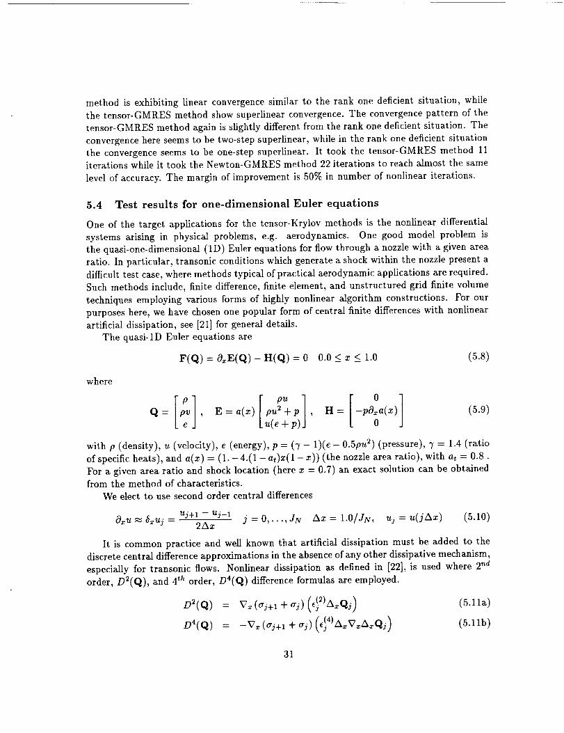
Figure 9: Results for 1D Euler using full nonlinear dissipation, Solid Line: tensor-GMRES;

Dotted-line: Newton-GMRES.

Boundary operators at j = 0 and j = JN are defined in terms of physical conditions

(taken from exact solution values) and the use of Riemann invariants. For this problem bothinflow and outflow boundaries are subsonic and locally one-dimensional Riemann invariants

are used. The locally one-dimensional Riemann invariants are given in terms of the velocity

component as

RI = u - 2c/('7 - l) and R2 = u + 2c/("/- 1). (5.12)

The Pdemann invariants R1, R2 are associated with the two characteristic velocities Az =

u - c and A2 = u + c respectively. One other equation is needed so that the three flow

variables can be calculated. We choose S = ln(p/p "v) where S is entropy. For subsonic

inflow u < c characteristic velocity As > 0 carrys information into the domain and therefore

the characteristic variable R2 can be specified along with one other condition. The Riemann

invariant R2, and S are set to exact values. The other characteristic velocity )_1 < 0 carriesinformation outside the domain and therefore, R1 is extrapolated from the interior flow

32

variables.On subsonicoutflow u < c and 12 > 0 carries information outside the domain,

while 11 < 0 propagates into the domain, so only R1 is fixed to exact values and R2, and

ln(S) are extrapolated. Once these three variables are available at the boundary the three

flow variables Q can be obtained. If we consider the boundary procedure as an operator on

the interior data, we can cast the boundary scheme as

B(q)i = Qi - B(Qi+I) = 0 i = 0

and

B(Q)i= Qi-B(Qi-1)=0 i= JN,

which are nonlinear equations at the boundaries.

=415E

-10

-12i i i i i i

2 3 4 5 6 7Iterdom

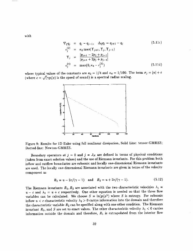
Figure 10: Results for 1D Euler using unlimited dissipation, Solid Line: tensor-GMRES;Dotted-line: Newton-GMRES.

The total system we shall solve is

{ if_E(Q)/- H(Q)/+ D_(Q) + D_(Q), j = 1,...,JNJ:(q) = B(Q)_ = 0, i= 0, JN

The Jacobian matrix for (5.13) is obtained in two ways. An approximated Jacobian is

formed analytically except, where due to the non-differential form of the _'s, the nonlinearcoefficients for the artificial dissipations, D 2 and D 4 are frozen at the linearized state,

i.e., they are not linearized. In another form, the Jacobian is obtained through a Frhchet

derivative, where error tolerances are appropriately chosen. The results presented below

are basicly independent of the choice of Jacobian linearization. The order of the system is

N = (JN + 1) × 3. A key element of the success of the solution using the Krylov subspace

methods is the choice of preconditioning. This issue for systems such as (5.13), which are

not diagonally dominate, is not straightforward and is still the subject of active research.

33

We shallnot go into the detail_of the preconditionerhere,and only state that the samepreconditioneris usedfor both the AlgorithmNG andTG sothat consistentcomparisonscanbe made.

O0

O7

!°°O5

01

O8-

OT-

i 05.

114-

025 05O 015

X

(a)

°3o6_

._t----

(b)

0S

O7O

X

O5

i

O4

J. 2Oz_

o3,

o 65025 050 o7_ 100

X

(c) (d)

o ro o z_

X

Figure 11: Pressure distribution: Solid Line: Computed; Dotted Line: Exact. (a) and (b)

Full Nonlinear Dissipation; (c) and (d) Unlimited Dissipation.

Figure 9 shows Algorithm NG and Algorithm TG applied to (5.13) for JN = 200;

N = 603. In the case of Algorithm NG the convergence appears linear taking approximately

125 steps to converge, while Algorithm TG shows about a factor of 6 decrease in the

number of nonlinear iterations and appears to be at least fast linear. To date, our analysis

indicates that the system derived form (5.13) is nonsingular and so we do not consider this

an example similar to the singular ones presented above. But, we have demonstrated, at

least numerically at this time, that the nondifferential nature of the nonlinear dissipation

coefficients in (5.11a-5.11d) is the source of the linear behavior observed. Figure 10 shows

the convergence results with g2 = 0, resulting in a quadratic-like convergence from both

Algorithm NG and TG. Nonlinear switching, such as defined in (5.11a-5.11d), is typical of

current numerical algorithms for the Euler and Navier-Stokes equations. They may take a

similar form to (5.1 la-5.11d), see [22] or be in the form oflimiters for upwind techniques, e.g.

[28],[16]. The nonlinear switching (limiting) is necessary to eliminate overshoots at shocks,

where higher order schemes are limited to lower order which more correctly differences the

34

equationsacrossdiscontinuities.Figure 11,showsthe resultswith and without limiting,noticethe overshootsacrossthediscontinuitywhicharemorepronouncedfor the unlimitedcase.In general,someform of limiting will be requiredandin thesecasesAlgorithm TGappearsto becapableof at leastfast linearconvergencein contrastto Algorithm NG'sslowlinear convergence.

5.5 Summary and discussion of test results

The test results of this section indicate that the tensor-GMRES algorithm that we tested

is more efficient in number of nonlinear iterations than the analogous Newton-GMRES

method on singular and nonsingular problems, and significantly more efficient on problemswhere the Jacobian matrix has a small rank deficiency at the solution or the function has

discontinuity. Since no failure was detected for either of the methods in the tests, it isinconclusive which method would be more robust. We observed that for each nonlinear

iteration, the number of restarts of the GMRES algorithm for solving the Newton equation

was ranging from 3 to 20 (recall that for all test problems the number of Arnoldi iterations

allowed in the GMRES algorithm was set to 20). As discussed in Section 4, in the tensor

algorithm the computation of the tensor step only uses the Krylov subspace that is produced

by the last restarted GMRES algorithm. Statistically, the size of the last Krylov subspacethat is used in the tensor model formation and solution is likely to be half of the number

of Arnoldi iterations allowed in the GMRES algorithm (for example 20/2 = 10 for our

tests). As analyzed in Subsection 4.7, the extra computational cost of each tensor iteration

is only a fraction of the cost of the last restarted GMRES algorithm. Hence for our test

problems (some of them are easy to solve), statistically, the extra cost of one tensor-GMRES

iteration would be ranging from 2.6% (when 20 restarts of GMRES were needed) to 20%

(when 3 restarts of GMRES were needed), compared to the cost of one Newton-GMRESiteration. In addition, from our experience the tensor-GMRES did not generate iterates

where the Newton equations would be harder to solve. Hence the savings of the tensor-

GMRES algorithm in number of nonlinear iterations can be roughly translated into savings

in overall computational costs, especially for problems where more restarts of the GMRES

algorithm were needed to solve the Newton equations. In general, at each iteration, themore restarts of the GMRES algorithm that are required for solving the Newton equation,

the lower the extra cost for a tensor-GMRES step. For real world problems, it is likely that

at each nonlinear iteration, the solution of the Newton equation would require a significant

number of restarts of the GMRES algorithm. Hence the extra cost of the tensor-GMRES

method is likely to be minimal in practice.

6 Summary and topics for future research

This paper has introduced the tensor-GMRES method for systems of nonlinear equations.

This method has similar requirement for storage and arithmetic per iteration to the Newton-

GMRES method. This method is also consistent with preconditioning and matrix free

35

implementation.An implementationof full nonlinear algorithm using the tensor-GMRES

method has shown to be more efficient on both nonsingular and singular problems than

analogous implementation of the Newton-GMRES method. The efficiency advantage ofthe tensor-GMRES method is particularly large on problems where the Newton-GMRES

method exhibits linear convergence (due to singularity or discontinuity).

Based on these results, it would appear worthwhile to continue research on tensor-Krylov

methods on nonlinear equations. The two main topics for future research would appear to be

practical implementation and farther testing of the tensor-GMRES methods for nonlinear

equations, and new tensor-Krylov methods for nonlinear equations. We discuss each of

these briefly.

As seen in Section 5, our implementation is still in early stage. Several directions

can be pursued immediately to improve the current implementation: (1) Scaling in both

the variable space and the function space can be added; (2) Matrix free implementation

of the tensor-GMRES method, which can be achieved in a fashion similar to analogous

implementation of the Newton-GMRES method, can be pursued; (3) More sophisticated

stopping criteria in the nonlinear algorithm can be included; (4) More global convergence

strategies such as model trust region techniques can be integrated. We would like to continue

our testing of the tensor-GMRES method on more practical problems. One interesting task

is to test the tensor-GMRES method on the ARC2D code [21] that is the two dimensionversion of the ARC1D code that we tested in Section 5.

Secondly, new tensor-Krylov methods can be developed. An immediate direction that

one can pursue is a tensor-Arnoldi method since the Arnoldi's method for linear systems is

closely related to the GMRES method for linear systems. A less straightforward direction

that can be pursued in the future is to combine tensor methods with Krylov methods

that use two mutually orthogonal sequences such as BiCG and QMR. We are currently

investigating this possibility.

Acknowledgement

We thank Prof. Bobby Schnabel for many helpful discussions related to this paper.

References

[1] W. E. ARNOLDI, The principle of minimized iteration in the solution of the matrix

eigenvalue problem, Quart. Appl. Math., 9 (1951), pp. 17-29.

[2] A. BOUARICHA, Solving large sparse systems of nonlinear equations and nonlinear

least squares problems using tensor methods on sequential and parallel computers, PhD

thesis, Department of Computer Science, University of Colorado, 1992.

[3] P. N. BROWN AND A. C. HINDMARStt, Reduced storage methods in stiff ODE systems,

J. Appl. Math. Comput., 31 (1989), pp. 40-91.

36

[4] P. N. BROWNAND Y. SAAD, Global convergent techniques in nonlinear Newton-

Krylov algorithms, Tech. Rep. 89.57, Research Institute for Advanced Computer Sci-

ence, NASA Ames Research Center, November 1989.

[5] _, Hybrid Krylov methods for nonlinear systems of equations, SIAM J. Sci. Stat.

Comput., 11 (1990), pp. 450-481.

[6] T. F. CIIAN AND K. R. JACKSON, The use of iterative linear equation solvers incodes .for large systems of stiff IVPs for ODEs, SIAM J. Sci. Stat. Comput., 7 (1986),

pp. 378-417.

[7] D. W. DECKER, H. B. KELLER, AND C. T. KELLEY, Convergence rate for Newton's

method at singular points, SIAM J. Numer. Anal., 20 (1983), pp. 296-314.

[8] D. W. DECKER AND C. T. KELLEY, Newton's method at singular points I, SIAM J.

Numer. Anal., 17 (1980), pp. 66-70.

[9] _, Newton's method at singular points II, SIAM J. Numer. Anal., 17 (1980), pp. 465-471.

[10] --, Convergence acceleration for Newton's method at singular points, SIAM J. Nu-

mer. Anal., 19 (1981), pp. 219-229.

[11] J. E. DENNIS JR. AND R. B. SCttNABEL, Numerical methods/or nonlinear equationsand unconstrained optimization, Prentice-Hall, Englewood Cliffs, NJ., 1983.

[12] D. FENG, Tensor methods for constrained optimization, PhD thesis, Department of

Computer Science, University of Colorado, 1993.

[13] D. FENG, P. D. FRANK, AND R. B. SCHNABEL, Local convergence analysis of tensor

methods for nonlinear equations, Mathematical Programming, 62 (1993), pp. 427-459.

[14] A. GRIEWANK, On solving nonlinear equations with simple singularities or nearly sin-

gular solutions, SIAM Review, 27 (1985), pp. 537-563.

[15] A. GRIEWANK AND M. R. OSBORNE, Analysis of Newton's method at irregular singu-

larities, SIAM J. Numer. Anal., 20 (1983), pp. 747-773.

[16] A. HARTEN, High resolution schemes/or hyperbolic conservation laws, J. Comp. Phys.,

49 (1983), pp. 357-393.

[17] C. T. KELLEY AND R. SURESIt, A new acceleration method/or newton's method at

singular points, SIAM J. Numer. Anal., 20 (1983), pp. 1001-1009.

[18] J. J. MOR_, A collection of nolinear model problems, Lectures in Applied Mathematics,

26 (1990), pp. 723-762.

37

[19] J. J. MORI_, B. S. GARBOW, AND K. E. HILLSTROM, Testing unconstrained opti-

mization software, ACM Transactions on Mathematical Software, 7 (1981), pp. 17-41.

[20] J. M. ORTEGA, Numerical Analysis, Academic Press, New York, 1972.

[21] T. H. PULLIAM, E.O_cient solution methods for the navier-stokes equations. Lecture

Notes for the yon K£rm£n Institute For Fluid Dynamics Lecture Series : Numerical

Techniques for Viscous Flow Computation In Turbomachinery Bladings, von K£rm£n

Institute, Rhode-St-Genese, Belgium , 1985.

[22] , Artificial dissipation models for the euler equations, hIiA J., 24 (1986),

pp. 1931-1940.

[23] G. W. REDDIEN, On Newton's method for singular problems, SIAM J. Numer. Anal.,

15 (1978), pp. 993-996.

[24] Y. SAAD AND M. H. SCHULTZ, GMRES: A generalized minimal residual algorithm for

solving nonsymmetric linear systems, SIAM J. Sci. Stat. Comput., 7 (1986), pp. 856-869.

[25] R. B. SCItNABEL AND A. BOUARICItA, Tensor methods for solving large sparse systems

of nonlinear equations and nonlinear least square problems. In preparation.

[26] R. B. SCHNABEL AND P. D. FRANK, Tensor methods for nonlinear equations, SIAM

J. Numer. Anal., 21 (1984), pp. 815-843.

[27] G. W. STEWART, Error and perturbation bounds for subspaces associated with certain

eigenvalue problems, SIAM Review, 15 (1973), pp. 727-764.

[28] P. K. SWEBY, High resolution schemes using flux limiters for hyperbolic conservation

laws, SIAM J. Num. Anaylsis, 21 (1984), pp. 995-1011.

38