Tension Monitoring of Toothed Belt DrivesUsing Interval-Based Spectral Features

Moritz Fehsenfeld ∗ Johannes Kuhn ∗∗ Mark Wielitzka ∗

Tobias Ortmaier ∗

∗ Leibniz University Hannover, Institute of Mechatronic Systems, Ander Universitat 1, 30823 Garbsen, Germany (e-mail:

fehsenfeld@imes.uni-hannover.de).∗∗ Lenze Automation GmbH, Am Alten Bahnhof 11, 38122

Braunschweig, Germany

Abstract: Toothed belt drives are used in manifold automation applications. But only if thebelt tension is properly adjusted, optimal working conditions are ensured. A loss of efficiencyor even breakdowns might be the consequences otherwise. For this reason, tension monitoringreduces operation costs and may prevent failures. In order to meet industrial requirements, themonitoring is supposed to rely on standard sensor data. From this data, features are extractedin time and frequency domain which are passed on to a random forest. For further improvement,a segmentation of the frequency spectrum is performed beforehand. In this way, interval-basedspectral features can be extracted to capture small distinctive parts in the frequency domain.For this purpose, two different segmentation procedures are compared in a random forestregression. A belt drive powered by a 1.9 kW synchronous servomotor is used to evaluate theproposed approaches in two different industrial scenarios. The experimental results show thatboth segmentation methods enhance the performance of a tree-based regression and offer areliable tension prediction.

Keywords: Fault detection and diagnosis, Machine learning, Industrial production systems,Time series modeling, Segmentation

1. INTRODUCTION

Condition monitoring is a widespread solution for manyindustrial applications to detect failures during operation.Monitoring of electrical drives mainly focuses on the motorwhere extensive work has been done to identify faulty con-ditions including bearing faults (e.g. Prieto et al. (2013)),rotor faults (e.g. Gyftakis et al. (2013)) and winding faults(e.g. Filho et al. (2014)). An overview of the field is givenby Riera-Guasp et al. (2015). However, failures in beltdrives can also force an entire production line to stop re-sulting in high expenses. But preventing downtimes is notthe only issue. To keep the wear of involved componentsat a minimum and to increase efficiency to a maximum,it is necessary to tension the belt properly. If pretensionis set too high, cord fatigue and tooth wear might bethe consequence. If the belt is too loose, the tooth loadincreases. Both cases lead to early failures and non-optimaloperation conditions. For this reason, a tension monitoringsystem helps to keep belt drives close to their optimalworking point.

1.1 Effects of Belt Tension on Measurement Data

The basis for distinction of different tension conditions isfinding patterns in the sensor data that are changing asthe belt tension is increased or decreased. In industrialapplications, the proper belt tension is determined by eval-uating the first mode natural frequency of the transverse

belt oscillations. When considering the belt as a vibratingstring, the belt tension F is given by

F = 4f2l2m. (1)

Besides the frequency f , the tension, therefore, depends onthe belt’s mass per length m and its length l. This rela-tionship is often used in fault detection and tension moni-toring, leading to the need to measure the belt’s transversefrequency during operation. Khazaee et al. (2017) andUcar et al. (2014) obtained vibration signals by employingan optical laser that captures the belt’s transverse motionto classify different failures. Musselman and Djurdjanovic(2012) utilized strain gauges to monitor belt tension. Huet al. (2016) capture belt oscillations using an electrostaticsensor. All these approaches require external sensors whichare not always available in industrial applications dueto cost and place restrictions. Therefore, it is desirableto build a monitoring system that only requires datafrom standard sensors. Motor current signature analysis(MCSA) is a very popular procedure in fault diagnosisbecause the motor current is commonly available. It is usedto classify belt failures like crack and wear by Kang et al.(2018). Picot et al. (2017) distinguish four different belttension levels based on motor current.

1.2 Principles of Belt Tension Monitoring

This work presents a data-driven procedure using conven-tional machine learning techniques to monitor the preten-sion of a toothed belt drive relying only on measurement

Preprints of the 21st IFAC World Congress (Virtual)Berlin, Germany, July 12-17, 2020

Copyright lies with the authors 756

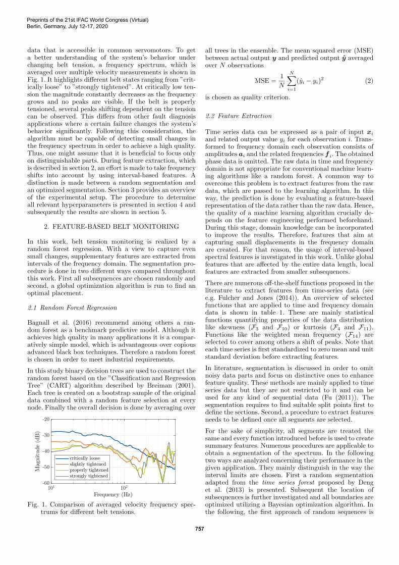
data that is accessible in common servomotors. To geta better understanding of the system’s behavior underchanging belt tension, a frequency spectrum, which isaveraged over multiple velocity measurements is shown inFig. 1. It highlights different belt states ranging from ”crit-ically loose” to ”strongly tightened”. At critically low ten-sion the magnitude constantly decreases as the frequencygrows and no peaks are visible. If the belt is properlytensioned, several peaks shifting dependent on the tensioncan be observed. This differs from other fault diagnosisapplications where a certain failure changes the system’sbehavior significantly. Following this consideration, thealgorithm must be capable of detecting small changes inthe frequency spectrum in order to achieve a high quality.Thus, one might assume that it is beneficial to focus onlyon distinguishable parts. During feature extraction, whichis described in section 2, an effort is made to take frequencyshifts into account by using interval-based features. Adistinction is made between a random segmentation andan optimized segmentation. Section 3 provides an overviewof the experimental setup. The procedure to determineall relevant hyperparameters is presented in section 4 andsubsequently the results are shown in section 5.

2. FEATURE-BASED BELT MONITORING

In this work, belt tension monitoring is realized by arandom forest regression. With a view to capture evensmall changes, supplementary features are extracted fromintervals of the frequency domain. The segmentation pro-cedure is done in two different ways compared throughoutthis work. First all subsequences are chosen randomly andsecond, a global optimization algorithm is run to find anoptimal placement.

2.1 Random Forest Regression

Bagnall et al. (2016) recommend among others a ran-dom forest as a benchmark predictive model. Although itachieves high quality in many applications it is a compar-atively simple model, which is advantageous over copiousadvanced black box techniques. Therefore a random forestis chosen in order to meet industrial requirements.

In this study binary decision trees are used to construct therandom forest based on the ”Classification and RegressionTree” (CART) algorithm described by Breiman (2001).Each tree is created on a bootstrap sample of the originaldata combined with a random feature selection at everynode. Finally the overall decision is done by averaging over

Fig. 1. Comparison of averaged velocity frequency spec-trums for different belt tensions.

all trees in the ensemble. The mean squared error (MSE)between actual output y and predicted output y averagedover N observations

MSE =1

N

N∑i=1

(yi − yi)2 (2)

is chosen as quality criterion.

2.2 Feature Extraction

Time series data can be expressed as a pair of input xi

and related output value yi for each observation i. Trans-formed to frequency domain each observation consists ofamplitudes ai and the related frequencies f i. The obtainedphase data is omitted. The raw data in time and frequencydomain is not appropriate for conventional machine learn-ing algorithms like a random forest. A common way toovercome this problem is to extract features from the rawdata, which are passed to the learning algorithm. In thisway, the prediction is done by evaluating a feature-basedrepresentation of the data rather than the raw data. Hence,the quality of a machine learning algorithm crucially de-pends on the feature engineering performed beforehand.During this stage, domain knowledge can be incorporatedto improve the results. Therefore, features that aim atcapturing small displacements in the frequency domainare created. For that reason, the usage of interval-basedspectral features is investigated in this work. Unlike globalfeatures that are affected by the entire data length, localfeatures are extracted from smaller subsequences.

There are numerous off-the-shelf functions proposed in theliterature to extract features from time-series data (seee.g. Fulcher and Jones (2014)). An overview of selectedfunctions that are applied to time and frequency domaindata is shown in table 1. These are mainly statisticalfunctions quantifying properties of the data distributionlike skewness (F3 and F10) or kurtosis (F4 and F11).Functions like the weighted mean frequency (F14) areselected to cover among others a shift of peaks. Note thateach time series is first standardized to zero mean and unitstandard deviation before extracting features.

In literature, segmentation is discussed in order to omitnoisy data parts and focus on distinctive ones to enhancefeature quality. These methods are mainly applied to timeseries data but they are not restricted to it and can beused for any kind of sequential data (Fu (2011)). Thesegmentation requires to find suitable split points first todefine the sections. Second, a procedure to extract featuresneeds to be defined once all segments are selected.

For the sake of simplicity, all segments are treated thesame and every function introduced before is used to createsummary features. Numerous procedures are applicable toobtain a segmentation of the spectrum. In the followingtwo ways are analyzed concerning their performance in thegiven application. They mainly distinguish in the way theinterval limits are chosen. First a random segmentationadapted from the time series forest proposed by Denget al. (2013) is presented. Subsequent the location ofsubsequences is further investigated and all boundaries areoptimized utilizing a Bayesian optimization algorithm. Inthe following, the first approach of random sequences is

Preprints of the 21st IFAC World Congress (Virtual)Berlin, Germany, July 12-17, 2020

757

Table 1. Functions to extract features from asignal of L and K samples respectively.

Time domain Frequency domain

F1 = 1L

∑L

i=1xi F8 = 1

K

∑K

i=1ai

F2 = 1L

∑L

i=1(xi −F1)2 F9 = 1

K

∑K

i=1(ai −F8)2

F3 =

∑L

i=1(xi−F1)

3

L·F32

F10 =

∑K

i=1(ai−F11)

3

k·F39

F4 =

∑L

i=1(xi−F1)

4

L·F42

F8 =

∑K

i=1(ai−F9)

4

K·F49

F6 = 1L

∑L

i=1|xi| F12 =

∑K

i=1a2i

F7 =

(1L

∑L

i=1

√|xi|)2

F13 =

∑K

i=1ai·fi∑K

i=1ai

referred to as random segmentation forest (RSF) and thelatter as optimized segmentation forest (OSF).

2.3 Random Segmentation Forest

The biggest issue when using interval-based features iswhere to split the sequential data. One easy way to do so isto randomly select boundaries. Deng et al. (2013) describean approach to create a time series forest (TSF) based onfeatures from random subsequences. As the name impliesit is a random forest approach where each tree is trainedon an individual set of interval-based features. Duringtraining stage, a set of b

√mc subsequences is defined

individually for each tree where m is the length of dataset.All split points are chosen randomly leading to differentfeatures as well. Summary functions are applied to everysubsequence to obtain local features. For comparability thesame feature functions described in table 1 are chosen.This leads to a set of 14 times b

√mc features which are

used to train each tree. For further information on thealgorithm refer to Deng et al. (2013).

There are two main hyperparameters to tune a TSFnamely the number of trees NT and the minimum intervallength Lmin. The number of trees influences the amountof intervals and by this the size of the related feature sets.Therefore, the computational time for feature extractionand regression learning increases as the number of treesgrows. To ensure a level of information in every subse-quence its minimum length Lmin can be set externally.

2.4 Optimized Segmentation Forest

A random splitting leads to a vast amount of differentintervals which are only evaluated during the randomforest training. In order to find an optimal solution withonly a few good intervals, the segmentation is expressedas an optimization problem. Each interval is defined bya starting point and an endpoint giving two parametersper section that need to be optimized. All points areonly constrained by the frequency range of the sampleddata. Since the location of a subsequence highly affectsthe features, the prediction result directly depends on itas well. Therefore, the quality of segmentation is evaluatedbased on the performance in a tree-based regression. Forthis reason, a random forest is trained and the meansquared error of a 3-fold cross-validation is calculatedto determine the loss of a parameter combination. A

Bayesian optimization algorithm (BOA) is used to runthe optimization. For information on the algorithm referfor example to Snoek et al. (2012). To avoid a high-dimensional parameter space only one subsequence isoptimized per run. The number is then gradually increasedby keeping previous subsequences constant. By this, theoptimization problem is split into numerous smaller onesleading to lower computational costs. On the other handthe performance is not found to be significantly lower thana one step optimization.

3. EXPERIMENTAL SETUP

The validation is conducted on a test bench depicted inFig. 2. It comprises of three triangularly arranged beltpulleys connected by a toothed belt (AT-5 profile) witha total length of l = 0.975 m. The lower right pulley islinked to a synchronous servomotor with a rated torqueof M0 = 5.5 Nm and a rated power of P0 = 1.9 kW. Thesetup’s control topology is characteristic of applications inautomation consisting of a programmable logic controller(PLC) and a servo inverter which feeds the motor. Theservomotor is equipped with an encoder to measure itsposition.

A roller can be moved up and down by a spindle driveallowing a continuous adjustment of the belt tension. Apotentiometer is attached to the spindle drive to measurethe roller’s position and thereby the distance used forpretension. At this point, it should be noted that measure-ment data obtained from the potentiometer is not used topredict the belt tension but for labeling purposes only.

3.1 Measurement Data

The data acquisition is done by a PLC at a frequency offs = 1000 Hz which is a typical setup in many industrialapplications. The employed servomotor is not equippedwith additional sensors and thus only provides data thatis available in off-the-shelf motors, which is:

• position (and derivatives),• torque and• temperature.

Because the belt tension can not be measured directly itis represented by the spindle drive’s position. The firstmode natural frequency of the belt transverse oscillationis acoustically measured to determine the tension based on(1). Although the belt’s behavior is non-linear the relationbetween position and belt tension can be linearly described

Fig. 2. Front view of the test bench.

Preprints of the 21st IFAC World Congress (Virtual)Berlin, Germany, July 12-17, 2020

758

(a) MFE (b) Jerk-limited trajectory

Fig. 3. Time domain representation of the excitations.

in the considered range. The position is be varied fromy = 0 cm (F ≈ 0 N) at the upper end of the potentiometerwhere the roller barely touches the belt to a maximum ofy = 5 cm (F = 230 N) where a tension higher than desiredis induced.

An excitation is needed to predict the actual belt tension.In general, any random motion that is applicable inan automation industry environment can serve for thispurpose. But the recorded time series data and by that theprediction quality highly depends on it. Furthermore theexcitation determines the operation conditions in practice.

Fault detection approaches can generally be divided intoactive and passive (see e.g. Puncochar and Skach (2018)).The excitations assessed throughout this work are chosenin a way that they cover both groups:

1. jerk-limited positioning trajectory (JLT)2. multifrequency sinusoidal excitation (MFE).

A jerk-limited trajectory is a typical positioning movementin industrial settings and is therefore available duringnormal operation. It consists of matching set values ofposition, velocity, and acceleration, that are generatedduring path planning. As a result, all available sensorsignals are logged during motion and the belt monitoringcan be done without disturbing the normal operation.

In the second scenario an auxiliary signal is injectedinto the system to evaluate the belt tension. For thispurpose a MFE signal is chosen, which is often used forparameter identification (see e.g. Evans et al. (1992)). It isa superposition of NF sinusoidal functions with differentangular frequency ωi and phase shift ϕi. The torque setvalue M(t) which is applied can be described by

M(t) =

NF∑i=1

sin(ωit+ ϕi). (3)

During the excitation the system’s velocity response isexamined leading to a time series with a fixed numberof samples that is used for feature extraction. Due toits design it excites many frequencies in a certain range.By that it is assured that the system characteristics arecomprehensively visible. A time-domain representation ofthe resulting torque for both excitations is depicted inFig. 3(a) and 3(b) to highlight the differences.

4. HYPERPARAMETER TUNING

This section focuses on the adaption of hyperparametersthat are directly connected to the extraction of interval-based features. All other parameters especially those ofunderlying decision trees are not tuned and globally keptconstant.

4.1 Random Segmentation Forest

The main parameters of a TSF are the number of treesand the minimum length of a subsequence. The maximumnumber of trees is set to NT = 20 to limit the compu-tational costs. A grid search over both parameters witha step size of ∆Lmin = 5 samples and ∆NT = 2 trees iscarried out. The results are shown in Fig. 4. In general, asmall number of trees leads to a slightly higher predictionerror while no significant tendency can be observed forthe minimum length. The minimum MSE is at a number ofNT = 14 trees and a minimum length of Lmin = 30 samplesand thus chosen as hyperparameter combination.

4.2 Optimized Segmentation Forest

The total number of subsequences is determined by grad-ually increasing it during segmentation optimization asdescribed in section 2.4. The quality is evaluated based onthe MSE that is achieved in a random forest regression.It can be seen from Fig. 5 that the MSE decreases asthe number of subsequences grows. The maximum numberof subsequences is set to Nseq = 10 because for bothexcitations no significant improvement is observed beyondthat point.

Since the loss function depends on the train-test split itis subject to scattering. Hence, the segment boundariesslightly vary from run to run but the overall performanceis almost constant. To illustrate the general optimizationresults a characteristic example segmentation is shown inFig. 6 for the MFE. The frequency spectrum shown atthe beginning in Fig. 1 is plotted to clarify the findings.The segment width ranges from small to almost across theentire spectrum. A concentration of starting and endpointscan be seen close to peaks in the spectrum which supportsthe initial intention to recognize their shift.

5. RESULTS OF TENSION MONITORING

The tension monitoring algorithms are tested under twoaforementioned excitations. In order to obtain meaningfulresults, the training, validation and test dataset are treatedseparately. Training and validation dataset are used formodel creation and determination of hyperparameters.The training dataset contains 900 measurements for bothexcitation movements. A uniform distribution over theoutput y is intended to eliminate data imbalances as a

50

100

150

200

250

300

350

Fig. 4. Result of the TSF hyperparameter grid searchwhere X marks the minimum.

Preprints of the 21st IFAC World Congress (Virtual)Berlin, Germany, July 12-17, 2020

759

(a) MFE (b) Jerk-limited Trajectory

Fig. 5. Investigation of the number of subsequences forinterval-based features.

reason for differences in performance. All results shown inthis section are based on the test dataset which is recordedseparately from the training. A random forest where allinterval features are omitted and only global features arekept is used as a reference to evaluate the interval-basedapproaches.

For the MFE a comparison of the actual output with thepredicted output for each sample in the test dataset isshown in Fig. 7. The reference results which are depictedin Fig. 7(a) show an occasional offset where the predictedvalue differs from the actual output. A further improve-ment can be observed for both segmentation forests shownin Fig. 7(b). Almost no deviation between predicted andactual output is visible resulting in a low MSE.

The MFE can be considered more suitable for monitoringsince it is optimized to excite a broad spectrum of frequen-cies while the JLT is simply a typical movement during op-eration in the automation industry. This is reflected in theachieved results depicted in Fig. 8. Especially the referenceperformance drops compared to the MFE as demonstratedin Fig. 8(a). Many predicted samples have a clear deviationfrom the actual value. Especially at lower belt tension alarger improvement compared to the reference is accom-plished for a JLT by employing a segmentation. At higherbelt tension several outliers remain in either case.

As pointed out earlier the quality varies due to differencesin the segmentation. Therefore, the results of 30 runsare determined and the mean and standard deviation aregiven in table 2 for both excitations. The active faultdetection approach of using a MFE leads to significantlybetter regression results in all cases. Even a global featureapproach yields a lower MSE than every procedure for aJLT. Furthermore it can be concluded that both segmenta-tion procedures lead to an improvement in both scenarios.The optimization (OSF) does not lead to a significant

Fig. 6. Distribution of optimized subsequences (gray) fora MFE.

(a) Reference algorithm with global features

(b) Segmentation forest with interval-based features

Fig. 7. Results of tension monitoring during MFE excita-tion.

performance gain but reduces the number of intervals(Nseq,OSF = 10) compared to the RSF (Nseq,RSF = 286)and the standard deviation of the MSE.

6. CONCLUSIONS

In this work, a segmentation procedure is proposed, whichwas tested in two industrial scenarios. A test bench wherethe belt tension can be adjusted is utilized to validate theapproaches. By applying a MFE the entire frequency rangeis excited and even a basic approach like a random forest

(a) Reference algorithm with global features

(b) Segmentation forest with interval-based features

Fig. 8. Results of tension monitoring during JLT excita-tion.

Preprints of the 21st IFAC World Congress (Virtual)Berlin, Germany, July 12-17, 2020

760

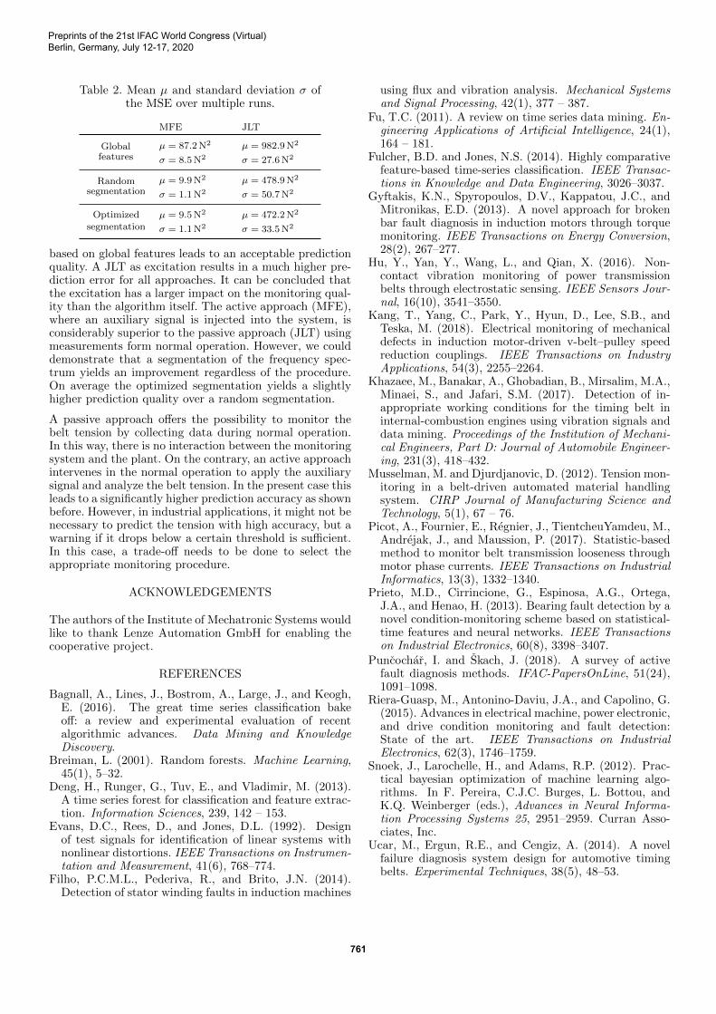
Table 2. Mean µ and standard deviation σ ofthe MSE over multiple runs.

MFE JLT

Globalfeatures

µ = 87.2N2 µ = 982.9N2

σ = 8.5N2 σ = 27.6N2

Randomsegmentation

µ = 9.9N2 µ = 478.9N2

σ = 1.1N2 σ = 50.7N2

Optimizedsegmentation

µ = 9.5N2 µ = 472.2N2

σ = 1.1N2 σ = 33.5N2

based on global features leads to an acceptable predictionquality. A JLT as excitation results in a much higher pre-diction error for all approaches. It can be concluded thatthe excitation has a larger impact on the monitoring qual-ity than the algorithm itself. The active approach (MFE),where an auxiliary signal is injected into the system, isconsiderably superior to the passive approach (JLT) usingmeasurements form normal operation. However, we coulddemonstrate that a segmentation of the frequency spec-trum yields an improvement regardless of the procedure.On average the optimized segmentation yields a slightlyhigher prediction quality over a random segmentation.

A passive approach offers the possibility to monitor thebelt tension by collecting data during normal operation.In this way, there is no interaction between the monitoringsystem and the plant. On the contrary, an active approachintervenes in the normal operation to apply the auxiliarysignal and analyze the belt tension. In the present case thisleads to a significantly higher prediction accuracy as shownbefore. However, in industrial applications, it might not benecessary to predict the tension with high accuracy, but awarning if it drops below a certain threshold is sufficient.In this case, a trade-off needs to be done to select theappropriate monitoring procedure.

ACKNOWLEDGEMENTS

The authors of the Institute of Mechatronic Systems wouldlike to thank Lenze Automation GmbH for enabling thecooperative project.

REFERENCES

Bagnall, A., Lines, J., Bostrom, A., Large, J., and Keogh,E. (2016). The great time series classification bakeoff: a review and experimental evaluation of recentalgorithmic advances. Data Mining and KnowledgeDiscovery.

Breiman, L. (2001). Random forests. Machine Learning,45(1), 5–32.

Deng, H., Runger, G., Tuv, E., and Vladimir, M. (2013).A time series forest for classification and feature extrac-tion. Information Sciences, 239, 142 – 153.

Evans, D.C., Rees, D., and Jones, D.L. (1992). Designof test signals for identification of linear systems withnonlinear distortions. IEEE Transactions on Instrumen-tation and Measurement, 41(6), 768–774.

Filho, P.C.M.L., Pederiva, R., and Brito, J.N. (2014).Detection of stator winding faults in induction machines

using flux and vibration analysis. Mechanical Systemsand Signal Processing, 42(1), 377 – 387.

Fu, T.C. (2011). A review on time series data mining. En-gineering Applications of Artificial Intelligence, 24(1),164 – 181.

Fulcher, B.D. and Jones, N.S. (2014). Highly comparativefeature-based time-series classification. IEEE Transac-tions in Knowledge and Data Engineering, 3026–3037.

Gyftakis, K.N., Spyropoulos, D.V., Kappatou, J.C., andMitronikas, E.D. (2013). A novel approach for brokenbar fault diagnosis in induction motors through torquemonitoring. IEEE Transactions on Energy Conversion,28(2), 267–277.

Hu, Y., Yan, Y., Wang, L., and Qian, X. (2016). Non-contact vibration monitoring of power transmissionbelts through electrostatic sensing. IEEE Sensors Jour-nal, 16(10), 3541–3550.

Kang, T., Yang, C., Park, Y., Hyun, D., Lee, S.B., andTeska, M. (2018). Electrical monitoring of mechanicaldefects in induction motor-driven v-belt–pulley speedreduction couplings. IEEE Transactions on IndustryApplications, 54(3), 2255–2264.

Khazaee, M., Banakar, A., Ghobadian, B., Mirsalim, M.A.,Minaei, S., and Jafari, S.M. (2017). Detection of in-appropriate working conditions for the timing belt ininternal-combustion engines using vibration signals anddata mining. Proceedings of the Institution of Mechani-cal Engineers, Part D: Journal of Automobile Engineer-ing, 231(3), 418–432.

Musselman, M. and Djurdjanovic, D. (2012). Tension mon-itoring in a belt-driven automated material handlingsystem. CIRP Journal of Manufacturing Science andTechnology, 5(1), 67 – 76.

Picot, A., Fournier, E., Regnier, J., TientcheuYamdeu, M.,Andrejak, J., and Maussion, P. (2017). Statistic-basedmethod to monitor belt transmission looseness throughmotor phase currents. IEEE Transactions on IndustrialInformatics, 13(3), 1332–1340.

Prieto, M.D., Cirrincione, G., Espinosa, A.G., Ortega,J.A., and Henao, H. (2013). Bearing fault detection by anovel condition-monitoring scheme based on statistical-time features and neural networks. IEEE Transactionson Industrial Electronics, 60(8), 3398–3407.

Puncochar, I. and Skach, J. (2018). A survey of activefault diagnosis methods. IFAC-PapersOnLine, 51(24),1091–1098.

Riera-Guasp, M., Antonino-Daviu, J.A., and Capolino, G.(2015). Advances in electrical machine, power electronic,and drive condition monitoring and fault detection:State of the art. IEEE Transactions on IndustrialElectronics, 62(3), 1746–1759.

Snoek, J., Larochelle, H., and Adams, R.P. (2012). Prac-tical bayesian optimization of machine learning algo-rithms. In F. Pereira, C.J.C. Burges, L. Bottou, andK.Q. Weinberger (eds.), Advances in Neural Informa-tion Processing Systems 25, 2951–2959. Curran Asso-ciates, Inc.

Ucar, M., Ergun, R.E., and Cengiz, A. (2014). A novelfailure diagnosis system design for automotive timingbelts. Experimental Techniques, 38(5), 48–53.

Preprints of the 21st IFAC World Congress (Virtual)Berlin, Germany, July 12-17, 2020

761