Temporary Workforce Planning with Firm Contracts: A Model ...

Hindawi Publishing CorporationMathematical Problems in EngineeringVolume 2011, Article ID 209693, 18 pagesdoi:10.1155/2011/209693

Research ArticleTemporary Workforce Planning withFirm Contracts: A Model and a SimulatedAnnealing Heuristic

Muhammad Al-Salamah

Industrial and Systems Engineering Program, King Fahd University of Petroleum & Minerals,Box 382, (KFUPM) Dhahran 31261, Saudi Arabia

Correspondence should be addressed to Muhammad Al-Salamah, [email protected]

Received 1 November 2010; Revised 7 December 2010; Accepted 8 January 2011

Academic Editor: Wei-Chiang Hong

Copyright q 2011 Muhammad Al-Salamah. This is an open access article distributed underthe Creative Commons Attribution License, which permits unrestricted use, distribution, andreproduction in any medium, provided the original work is properly cited.

The aim of this paper is to introduce a model for temporary staffing when temporary employmentis managed by firm contracts and to propose a simulated annealing-based method to solve themodel. Temporary employment is a policy frequently used to adjust the working hour capacity tofluctuating demand. Temporary workforce planning models have been unnecessarily simplified toaccount for only periodic hiring and laying off; a company can review its workforce requirementevery period and make hire-fire decisions accordingly, usually with a layoff cost. We present amore realistic temporary workforce planning model that assumes a firm contract between theworker and the company, which can extend to several periods. The model assumes the traditionalconstraints, such as inventory balance constraints, worker availability, and labor hour mix. Thecosts are the inventory holding cost, training cost of the temporary workers, and the backordercost. The mixed integer model developed for this case has been found to be difficult to solve evenfor small problem sizes; therefore, a simulated annealing algorithm is proposed to solve the mixedinteger model. The performance of the SA algorithm is compared with the CPLEX solution.

1. Introduction

Temporary employment has been advocated as a means of flexible employment by whichcompanies can effectively adjust the workforce level when faced by fluctuating demand[1, 2]. Most manufacturing companies, such as, and especially, in hi-tech industry, face thefrequently occurring problem of manpower planning. Production planners need to planthe production by determining the delivery dates and invested capital, and one of themost important and most serious planning activities is the planning of the workforce sizeneeded to meet the production demands. Manpower planning is not an easy task given

2 Mathematical Problems in Engineering

the high costs involved. Most of these companies revert to temporary employment to absorband accommodate short-term requirements for manpower. Essentially, manpower planning,among many things, tries to obtain the right mix of company-owned workers who have lowsetup costs and high variable costs and contracted workers who have high setup costs andlow variable costs. The significance of the problem comes from the fact that this problemconfronts the hardware-assembly industry, such as the PC assembly companies in SaudiArabia.

These manufacturing companies have fixed capital investments in productionequipment; hence their fixed costs are primarily a function of the workforce size. Short-termemployment entails two expenses a company should be willing to pay: the training cost andnonproductive pay. At the beginning of the contract, contracted workers will go through atraining period during which they are not carrying out any productive work. The workercontracts are considered to be firm and the worker has to serve and will be paid for theduration of the contract. The contract covers the training period, which typically lasts for asmall fraction of the duration of the contract.

These PC assembly companies hire workers with technical college degrees, who areskilled in the technical matters of assembly of electronic components and wiring. When thoseworkers are hired on temporary contracts, they receive training on the assembly proceduresin the plant, and, because of their technical background, the workers pick up the work veryquickly and become as skillful as the regular workers. Other tasks, such as packaging anddelivery, do not require a technical background, and the workers hired for these tasks aretrained on the production procedures of the company, and they can master these tasks in avery short period of time.

A typical PC assembly plant has the design shown in Figure 1. The PC assemblyprocess consists of three main stages. The first stage is the assembly stage, where thecomponents of the PC are assembled and added to the PC case. The finished cases aredelivered to the next stage, which is the software installation stage. In this stage, the hardwareis tested before the software can be installed. Then, the cases are taken to the final stage,which is packaging. From packaging, the PC units are delivered to storage. The two stagesthat require technical education are the assembly and software installation stages, which canonly be fulfilled by workers with a technical college education.

The forms and types of temporary employment vary across countries and industriesaccording to employment laws and manpower needs and strategies [3]. In the majorEuropean countries, the duration of the contract can range from twelve months to anunlimited period, with provisions for repeated contracts [4].

The labor laws in the Kingdom have a provision for temporary employment. The lawspermit firms and companies to employ workers on a nonpermanent basis for a specific periodor for the duration of a particular job. The Labor Law (LABOR LAW, Royal Decree no. M/51,27 September 2005, https://mol.gov.sa/en/Pages/LaborLaw.aspx, accessed on November 5,2010) created by the Royal Decree no. M/51 defines temporary work as follows:

Work considered by its nature to be part of the employer’s activities, thecompletion of which requires a specific period or relates to a specific job and endswith its completion. (Labor Law, 2005, page 7)

The law hence permits companies to engage in temporary work that would requiretemporary employment. Under this law companies are not limited to a specific number oftemporary workers, and the law does not limit the applicability of temporary employmentcontracts to specific types of jobs. As stated in the Labor Law, the provisions and laws apply

Mathematical Problems in Engineering 3

Workstations

Parts

Assembly stage

WorkstationsDeliverysystem

Softwareinstallation stage

Deliverysystem

Packaging stageDeliverysystem

Storage

Figure 1: PC assembly process.

to any contract whereby a person commits himself to work for an employer and under hismanagement or supervision for a wage. However, the law under Article 26 of Chapter 1,Part II, puts restrictions on the manner in which workers are recruited, and, in fact, firms arerequired to have plans for the nationalization of jobs. The article states that firms, regardlessof their number of workers, should exert every effort to attract and employ nationals, provideconditions to keep them in the job, and avail them of an adequate opportunity to prove theirsuitability for the job by guiding, training, and qualifying them for their assigned jobs. Thearticle also requires firms to let the share of nationals in the total employed be no less thanseventy-five per cent.

Article 6 of Chapter 2 of Part I of the Labor Law identifies the provisions that arerelated to temporary workers. The article states that temporary workers are subject tothe provisions on duties and disciplinary rules, the maximum working hours, daily andweekly rest intervals, overtime work, official holidays, safety rules, occupational health, workinjuries, and compensation as well as other provisions that are decided by the Ministry ofLabor. Under this article, temporary workers have the same privileges and responsibilitiesas regular workers. In terms of workload, a worker may not work for more than eight hoursa day on a daily basis or more than forty-eight hours a week on a weekly basis. During themonth of Ramadan, the actual working hours for Muslims is reduced to a maximum of sixhours a day or thirty-six hours a week (Article 98, Chapter 2, Part VI). In special cases, thenumber of working hours can be raised to nine hours a day or reduced to seven hours (Article99, Chapter 2, Part VI).

The law specifies the rest times for workers as a matter of duration and timing. By law,workers should have a break at every five hours at a minimum, and the break should not lastfor less than thirty minutes. In terms of work duration, the daily workload should not exceedeleven hours. Workers should be compensated for overtime working hours by an additionalamount equal to the hourly wage plus fifty per cent of the basic wage (Articles 101 and 107,Chapter 3, Part VI). The law specifies the duration of the temporary employment. Article 2of Chapter 1, Part 1, declares that temporary employment contracts should not exceed ninetydays. Implicit in this law is the possibility of contract renewal.

Traditional periodic workforce review models permit planners to adjust the workforcelevel every period, with the flexibility to hire temporary workers without long-term


commitment; in most cases, a layoff cost is incurred. This flexibility may not always beavailable to a company; laws, as explained above, or the company’s own policies mayimpose fixed-term contracts. We offer an alternative formulation of the traditional temporarymanpower planning model with fixed contract duration that can extend to several timeperiods.

2. Literature on Periodic Workforce Review Models

The literature on temporary employment management can be classified as in the following:work commitment (i.e., [4–7]), worker attitude (i.e., [8, 9]), economics of temporaryemployment (i.e., [10–13]), and worker accident (i.e., [14, 15]). Traditionally, humanmanagement decisions have been solved using optimization mathematical models. Recently,many mathematical models have been proposed that would evaluate in economic terms thebenefits of temporary employment and find the optimal mix of the regular and temporaryworkforce. Some notable periodic review models on temporary employment include Bermanand Larson [16], Herer and Harel [17], Pinker and Larson [18], and Techawiboonwong et al.[19]. An extensive review of research related to temporary workers is reported by Connellyand Gallagher [7]. Generally, mathematical models are constructed to optimize a measure ofbenefit or load, subject to workload demand and manpower balance constraints.

Lee and Vairaktarakis [20] have studied a class of serial assembly system lines whichare formed by arranging several production cells or stations in series where all stationshave the same production cycle. The developed model will find a sequence of n job, whichminimizes the maximum workforce requirements over all production cycles.

Foote and Folta [10] studied the use of temporary workers as an option for a workforceexpansion decision. They concluded that there must be a particular reason for a tradeoffbetween these two types of workers. Kandel and Pearson [6] studied the optimal balancebetween permanent employment and temporary contracts between a firm and its workers:the tradeoff between higher productivity on the one hand and flexibility on the other.Through an examination of the optimal policy using an irreversible investment model,they found that higher expected growth in demand implies increases in the proportion ofpermanent workers, while an increase in the variability of demand lowers their proportion.An increase in the absolute cost advantage of the permanent workers naturally increases theiroptimal proportion in the labor force.

Wirojanagud et al. [21] developed a mixed integer programming model to determinethe amount of hiring, firing, and cross-training in a staffing decision problem, in whichworkers are inherently different, to minimize the total costs, which include training, salary,firing, and missed production costs over multiple time periods.

Song and Huang [22] considered the planning problem of transferring, hiring, orfiring employees among different departments or branches of an organization under anenvironment of uncertain workforce demands and turnover, with the objective of minimizingthe expected cost over a finite planning horizon. The organization could transfer theemployees from one department to another, hire, or fire employees to meet the workforcedemands, under the conditions that there may be constraints on the number of employeesthat could be transferred, hired, or fired in each period.

Techawiboonwong et al. [19] studied temporary employment in a labor-intensiveindustry. To aid the decision makers, an MIP model was proposed to determine the type(skilled or unskilled) and the number of temporary workers to hire or lay off in each period.


The skill levels are mandated by the nature of the manufacturing process. In this treatmentof the problem, temporary workers can be laid off in any period but there is a cost associatedwith the layoff. It is assumed that the pool of regular workers is cross-trained, and thereforethey are not restricted to being assigned only to specific workstations.

3. A Temporary Employment Model with Extended Contract Durations

We model the temporary employment planning problem with fixed-term temporaryemployment contracts that can extend to several periods as an MIP model. We argue thatfirms can lower their workforce-related costs if they adopt a fixed-term contract policy. Theassumptions of the model are illustrated next. Training is required for temporary workers;but we assume, from an observed case, that temporary workers, after training, become asskillful as regular workers and that their performance is comparable to those of the regularworkers when considering important manufacturing variables such as quality, scrap rate,and setups. This assumption holds true especially in the case presented earlier of the PCassembly process, in which temporary workers have a technical degree education and, whenthey are hired, receive training on the internal procedures of the company and the assemblyprocess, which can be mastered very quickly. Therefore, we assume that the training periodis negligibly short. For the sake of a wider coverage of the problem described here and allsimilar problems, we consider a multiproduct, multistage manufacturing/assembly process.

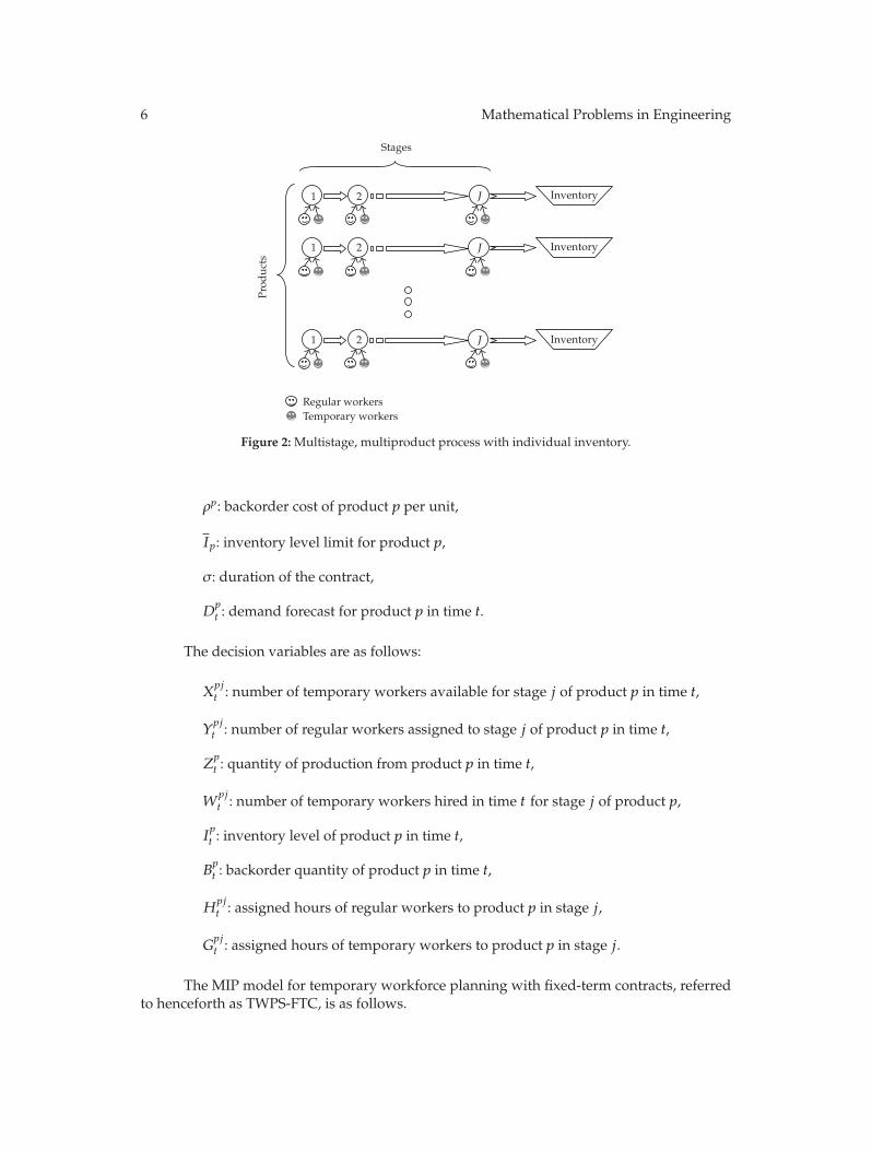
The manufacturing/assembly process under consideration is illustrated in Figure 2.This general process consists of a number of production lines: each line is for a specificproduct. Each line has a number of manufacturing/assembly stages. Every product line isequipped with an individual inventory. Regular workers are cross-trained and they can befreely assigned to stages and product lines. Each stage of any line can be operated by apool of regular and temporary workers. While regular workers are cross-trained, temporaryworkers are hired for specific tasks and stages. This assumption is close to the case of the PCassembly process, in which temporary workers are hired to perform specific jobs. Followingthe assumption of Techawiboonwong et al. [19], work in process is not considered.

Unlike the model by Techawiboonwong et al. [19], our MIP model does not havethe flexibility of overtime allowance. In our manufacturing/assembly process, there are Pproduct lines; for each line, there are J stages or workstations. Let p and j be the indices forproduct and stage, respectively. The length of the planning horizon is T, and t is the timeindex. Define the following parameters:

μpj : unit processing time for product p in stage j,

κt: production time in period t,

αj , βj : labor productivity rating of temporary and regular workers, respectively,

Y : total regular workers,

λpj : wage of temporary worker assigned to stage j of product p,

δpj : training cost of temporary worker assigned to stage j of product p,

ξp: inventory holding cost of product p per period,


1 2 J Inventory

1 2 J Inventory

1 2 J Inventory

Stages

Regular workersTemporary workers

Prod

ucts

Figure 2: Multistage, multiproduct process with individual inventory.

ρp: backorder cost of product p per unit,

Ip: inventory level limit for product p,

σ: duration of the contract,

Dpt : demand forecast for product p in time t.

The decision variables are as follows:

Xpjt : number of temporary workers available for stage j of product p in time t,

Ypjt : number of regular workers assigned to stage j of product p in time t,

Zpt : quantity of production from product p in time t,

Wpjt : number of temporary workers hired in time t for stage j of product p,

Ipt : inventory level of product p in time t,

Bpt : backorder quantity of product p in time t,

Hpjt : assigned hours of regular workers to product p in stage j,

Gpjt : assigned hours of temporary workers to product p in stage j.

The MIP model for temporary workforce planning with fixed-term contracts, referredto henceforth as TWPS-FTC, is as follows.


TWPS-FTC:

minT∑

t=1

⎧⎨

⎩

P∑

p=1

⎧⎨

⎩

J∑

j=1

{λpjX

pjt + δpjWpj

t

}+ ξpIpt + ρ

pBpt

⎫⎬

⎭

⎫⎬

⎭

subject to

(3.1)

Xpjt =

t∑

τ=t−σ+1

Wpjτ ∀t, p, j, (3.2)

Ipt − B

pt = Ipt−1−B

p

t−1 + Zpt −D

pt ∀t, p, (3.3)

Ipt ≤ Ip ∀t, p, (3.4)

Zpt μ

pj ≤ Hpjt +Gpj

t ∀t, p, j, (3.5)

Xpjt ≥ α

j Gpjt

κt∀t, p, j, (3.6)

Ypjt ≥ β

j Hpjt

κt∀t, p, j, (3.7)

J∑

j=1

P∑

p=1

Ypjt ≤ Y ∀t, (3.8)

Xpjt , Y

pjt , Z

pt ,W

pjt , I

pt , B

pt ∈ {0, 1, 2, . . .} ∀t, p, j,

Hpjt , G

pjt ≥ 0 ∀t, p, j.

(3.9)

The objective function consists of the temporary employment wages, training costs oftemporary workers, inventory holding costs, and backorder costs. Constraint set (3.2) ensuresthat the number of available temporary workers in time t is equal to the number of temporaryworkers hired in the current period and those whose contracts end in the current period, andall the temporary workers in between. As initial values, Wpj

−1 = Wpj

−2 = 0 for all p and j.Since hiring a temporary worker whose contract duration is going to extend beyond the endof the planning horizon is not permissible, we require Wpj

t = 0 for t = T − σ + 2, . . . , T forall p and j. Constraint set (3.3) is the set of inventory balance constraints. We impose therestriction that there should not be a backorder in the last period; hence, BpT = 0 for all p. Theinventory capacity constraint is managed by constraint set (3.4). Constraint set (3.5) restrictsthe production hours to the available temporary and regular worker hours. Constraint sets(3.6) and (3.7) ensure the availabilities of temporary and regular workers to meet the plannedproduction hours, respectively. The level of the regular workforce is imposed by constraint(3.8).

4. Simulated Annealing Solution Approach

The model TWPS-FTC has 3(|J | + 1)|T | |P | integer variables, where | · | is the cardinality ofthe set. Even for relatively small problems, MIP models are hard to solve to optimality.


The simulated annealing heuristic has been successfully applied to manpower planning, suchas that mentioned by Brusco and Jacobs [23, 24], Thompson [25], Ahire et al. [26], Lim et al.[27], Li et al. [28], Seckiner and Kurt [29], and others. The simulated annealing heuristic thatis proposed here to solve TWPS-FTC generates an all feasible solution in every run of theheuristic. The SA heuristic has only two free variables to change: assignment set of regularworkers (Ypj

t variables) and the production set (Zpt variables). Therefore, the dependent

variables Xpjt , Wpj

t , Ipt , Bpt , Hpjt , and G

pjt are calculated from the determined sets.

The simulated annealing algorithm proposed to solve TWPS-FTC requires four rules.The first rule specifies the generation of the initial assignment set of regular workers and theproduction set. This rule is required to start the simulated annealing algorithm. The secondrule specifies the way the neighborhood solution is generated from the current solution.The third rule specifies the generation of a feasible solution. The fourth rule determines theacceptance criterion of a solution and the termination criterion of the algorithm.

In the following subsections, we will explain how the initial sets are generatedrandomly and we show how the values of Xpj

t , Wpjt , Ipt , Bpt , Hp

t , and Gpjt are generated so that

the generated solution becomes feasible. The main steps of the SA algorithm can be outlinedas follows.

(1) Generate a random initial set.

(2) Generate a feasible solution.

(3) Loop until the stopping criterion is satisfied:

(a) generate a neighborhood solution,(b) generate a feasible solution,(c) evaluate the fitness function,(d) compare and accept or reject the new solution.

The fact that the production assignment determines inventory and backorder values [30] willmake it possible to generate a feasible solution, as will be explained in the following sections.

4.1. Generation of the Initial Assignment Set of Regular Workers

In each period of the planning horizon, the company has Y regular workers to assign tothe different product lines and stages. The initial assignment set of the regular workers canbest be generated randomly. The following steps illustrate the mechanism for the randomgeneration of the assignment set.

(1) Start with the first period in the planning horizon.

(2) Repeat until all regular workers are assigned:

(a) randomly choose a product line and a stage,(b) assign to the chosen product line and stage one regular worker. If regular

workers have been assigned to this particular line stage before, add thisworker to the existing workers.

(3) Advance to the next period, and repeat step (2) until the last period of the planninghorizon is covered.


j∗∗ j∗

p∗∗

p∗

t = t∗

Figure 3: Generation of a neighborhood solution.

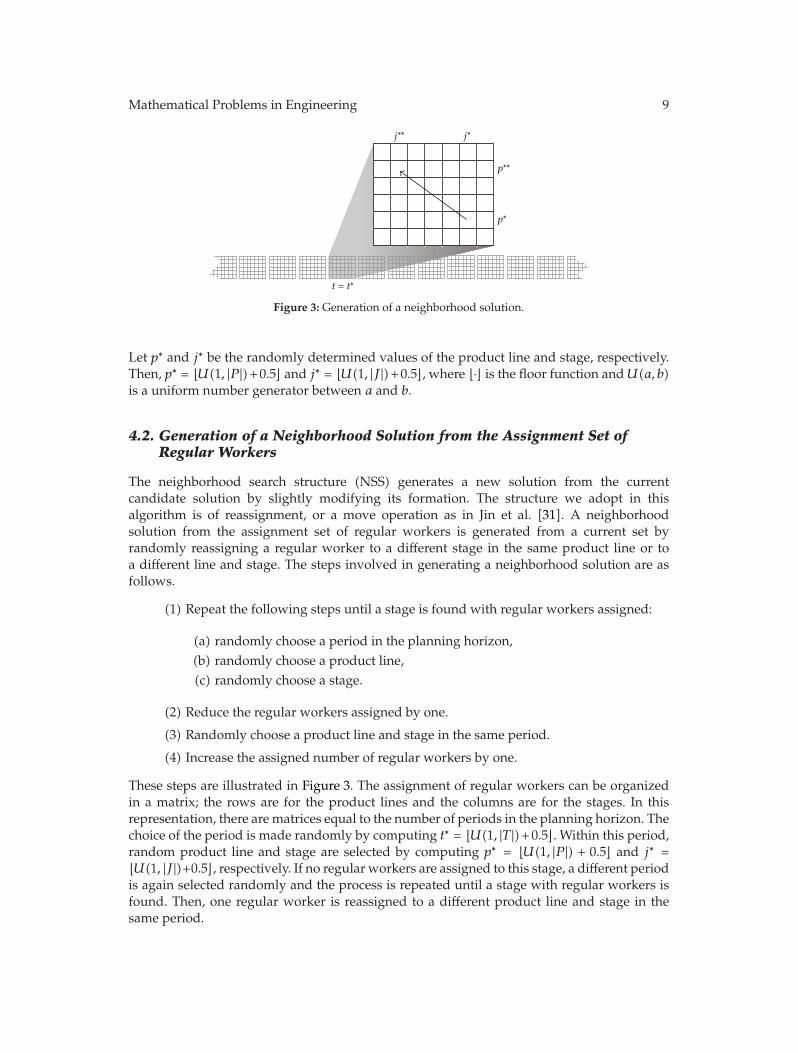
Let p∗ and j∗ be the randomly determined values of the product line and stage, respectively.Then, p∗ = �U(1, |P |)+0.5� and j∗ = �U(1, |J |)+0.5�, where �·� is the floor function and U(a, b)is a uniform number generator between a and b.

4.2. Generation of a Neighborhood Solution from the Assignment Set ofRegular Workers

The neighborhood search structure (NSS) generates a new solution from the currentcandidate solution by slightly modifying its formation. The structure we adopt in thisalgorithm is of reassignment, or a move operation as in Jin et al. [31]. A neighborhoodsolution from the assignment set of regular workers is generated from a current set byrandomly reassigning a regular worker to a different stage in the same product line or toa different line and stage. The steps involved in generating a neighborhood solution are asfollows.

(1) Repeat the following steps until a stage is found with regular workers assigned:

(a) randomly choose a period in the planning horizon,(b) randomly choose a product line,(c) randomly choose a stage.

(2) Reduce the regular workers assigned by one.

(3) Randomly choose a product line and stage in the same period.

(4) Increase the assigned number of regular workers by one.

These steps are illustrated in Figure 3. The assignment of regular workers can be organizedin a matrix; the rows are for the product lines and the columns are for the stages. In thisrepresentation, there are matrices equal to the number of periods in the planning horizon. Thechoice of the period is made randomly by computing t∗ = �U(1, |T |)+0.5�. Within this period,random product line and stage are selected by computing p∗ = �U(1, |P |) + 0.5� and j∗ =�U(1, |J |)+0.5�, respectively. If no regular workers are assigned to this stage, a different periodis again selected randomly and the process is repeated until a stage with regular workers isfound. Then, one regular worker is reassigned to a different product line and stage in thesame period.


4.3. Generation of the Initial Set of the Production

The only requirement for a production plan to be feasible is that the sum of the productionsin all periods is equal to the sum of demands in all periods for a specific product;mathematically, we have to have

∑Tt=1 Z

pt =

∑Tt=1 D

pt for product p. As an initial feasible

solution, the sum of the demands can be distributed evenly throughout the periods.

4.4. Generation of a Neighborhood Solution from the Production Set

In generating a neighborhood solution from the production set, we apply a load transferoperation. For a random period and random product, a random production quantityis transferred and loaded into another period’s production. Assume that t∗ and p∗ aregenerated randomly; generate RandomQuantity = �U(1, Zp∗

t∗ ) + 0.5�. Make Zp∗

t∗ = Zp∗

t∗ −RandomQuantity, generate another t∗∗; and make Zp∗

t∗∗ = Zp∗

t∗∗ + RandomQuantity.

4.5. Generation of Inventory and Backorder Sets

The production set determines the inventory Ipt and backorder Bpt sets. We apply a look-aheadmechanism for computing the inventory and backorder. Any backorder quantity representsan additional demand that is put into a future period, and inventory serves as extendedproduction capacity that will be available in a future period.

We apply the following steps to compute the inventory and backorder for a givenproduction set.

(1) Initialization: set p = 1, and set inventory and backorder to zero for all productsand periods.

(2) While p ≤ P , do

(i) Initialization: t = T(ii) While t > 1, do

(1) Compute Δpt = Z

pt −D

pt

(2) Check

(a) If Δpt < 0, set Ipt−1 = |Δp

t |(b) Else if Δp

t > 0, set Bpt−1 = Δpt

(c) Else, do not change Ipt and Bpt

(3) Decrement t by 1

(iii) End while

(b) Increment p by 1.

(3) End while.

4.6. Generation of Regular Labor Hours and Temporary Labor Hours

The regular labor hours are determined from the regular labor assignment set, which isdetermined by the generation steps in regular worker assignment set. The regular labor


hours are computed by reversing constraint (3.7), so that we can write that the regular laborhours in time t, product line p, and stage j are Hpj

t = (κt/βj)Ypjt . Constraint (3.5) defines the

relationship between the demand hours, regular worker hours, and temporary labor hours,so we can write Gpj

t = max(0, Zpt μ

pj −Hpjt ), for all t, p, and j.

4.7. Generation of Temporary Worker Utilization Plan Set and TemporaryWorker Hiring Set

From the temporary worker hours, we can calculate the number of temporary workersrequired to meet the production demands. The number of temporary workers needed inperiod t, product line p, and stage j is Xpj

t = ceiling [αj(Gpjt /κt)].

When the temporary worker utilization plan set is determined, the temporary workerhiring set can be determined. In the long-term contract agreement, additional temporaryworkers are hired only when previously hired temporary workers who are still within thecontract validity are not adequate to meet the production demands. Hence, the number oftemporary workers that have to be hired in the current period t is merely the differencebetween the required temporary workers in period t and the total hired workers in theinterval [t − σ + 1, t − 1]. We can write that Wpj

t = max(0, Xpjt −

∑t−1τ=t−σ+1 W

pjτ ) for all t, p,

and j. It is assumed for convenience that Wpj

−1 =Wpj

−2 = · · · = 0.

4.8. The Fitness Function

In simulated annealing algorithms, the fitness function is usually defined by the objectivefunction of the underlying model, as in the studies by Chen and Shahandashti [32], He et al.[33], and Sayarshad and Ghoseiri [34]. In our proposed simulated annealing algorithm, thefitness function is defined by the objective function in model TWPS-FTC.

4.9. Acceptance of a Solution and Termination of the Algorithm

In simulated annealing, a neighborhood solution is accepted in two conditions: theneighborhood solution is better than the best solution in the current iteration or else it isaccepted with some probability. If the neighborhood solution is not accepted, it is discardedand a new neighborhood solution is generated. In our simulated annealing algorithm, thereare two independent decision variables: the regular worker assignment Ypj

t and productionZpt . This situation causes a difficulty because generating a neighborhood solution that is a

combination of two generated neighborhood solutions is intractable; the improvement in thefitness function cannot be attributed to a single neighborhood solution; and the improvingneighborhood solution cannot be known. Therefore, we propose a two-stage procedure thatwill systematically generate a tractable neighborhood solution.

The two-stage procedure calls for the arbitrary selection of either regular workerassignment or production to be in the first stage in the procedure. The first stage will generatea neighborhood solution for the first variable and pass it to the second stage where several


neighborhood solutions are generated for the second variable before the execution returns tothe first stage where a new neighborhood solution for the first variable is generated. Howmany neighborhood solutions have to be generated in the second stage is a decision variableand only through experimentation can the best value be determined.

Simulated annealing was formally introduced in 1983 by Kirkpatrick et al. [35] to solvecombinatorial optimization problems. It is motivated by an analogy between combinatorialoptimization and physical annealing. Metals are first heated to a temperature that permitsmany molecules to move freely with respect to each other, then they are cooled slowly untilthe material freezes into a completely ordered form. In combinatorial optimization, simulatedannealing techniques use an analogous cooling operation for transforming a poor, unorderedsolution into an ordered, desirable solution, so as to optimize the objective function.

The outer loop of the simulated annealing algorithm is terminated when a specificnumber of iterations are consumed. In each iteration of the algorithm, a randomneighborhood solution is generated; if its fitness is better than the fitness of the currentsolution, it is accepted; otherwise it is accepted with a probability that is a function of theannealing temperature.

The literature lists many temperature cooling schemes [36]. In our simulatedannealing algorithm, we apply the cooling scheme TEMPi+1 = TEMPi/(1 + γTEMPi), whereβ is called the cooling rate, which controls the speed at which the temperature falls [31]. Thevalue given to β should be chosen carefully so that the temperature does not drop to zeroprematurely; values that are close to zero will make the drop very slow. Again, the choice ofβ can be determined by experimentation.

4.10. The Simulated Annealing Algorithm

Our simulated annealing algorithm starts by randomly generating initial sets of regularworkers and production. At the beginning, both the local and the global best solutions are setto the initial solution. A neighborhood solution, based on the outlined procedures in Sections4.2, 4.4, and 4.9, is generated; this solution is temporarily accepted when it is better then thebest local solution, or else it is accepted with some probability, which is influenced by thecooling temperature. The mainstream in simulated annealing research talks about updatingthe temperature in every run of the algorithm whether there has been a successful move.However, we propose that the temperature is updated only when the local solution has beenchanged; this mechanism will prevent the temperature from being unnecessarily reducedand prematurely too small. The algorithm is terminated when the loop counter exceeds aprespecified limit.

Define Yi = {Ypjt } to be the assignment set of regular workers in iteration i, Zk

i = {Zpt }

to be the production set in step k of the two-step procedure as explained in Section 4.9 initeration i, OBJki to be the fitness in iteration i, OBJlocal

i to be the fitness of the local solutionin iteration i, OBJglobal to be the fitness of the global solution, Y local

i to be the local assignmentset in iteration i, Y global to be the global assignment set, Zlocal

i to be the local production setin iteration i, and Zglobal to be the global production set. The counter limit is set to imax. Thesteps of the algorithm are explained in the following procedure.

Simulated Annealing Algorithm

Step 1. Initialization step: set the outer loop counter i = 1 and cooling temperature T1 = T0.


×10350040030020010010

Initial temperature T0

108

109

110

111

112

113

114

115

116×103

Bes

tcos

t

Figure 4: The initial temperature T0 versus optimal cost.

151051

kmax

108

109

110

111

112

113

114

115

116×103

Bes

tcos

t

Figure 5: Value of kmax versus optimal cost.

Table 1: Monthly demands.

Month PC Model1 2 3

1 720 210 6402 370 790 5003 1000 540 10004 230 390 4505 760 490 4506 830 440 9807 930 930 9008 320 250 3609 690 1000 21010 750 460 59011 360 830 52012 350 970 580

Table 2

Hardware assembly 11.7 minutesSoftware installation 5 minutesPackaging 3.5 minutes


Table 3

Stage Productivity1 1.12 1.053 1.03

Table 4

Contract duration 3 monthsAvailable regular workers 3Inventory limit for every model 1000 units

Step 2. Generate initial sets Y0 and Z01 as outlined in Sections 4.1 and 4.3. Generate the

inventory and backorder sets as in Section 4.5, the regular labor hours and temporary laborhours as in Section 4.6, and the temporary worker utilization plan set and temporary workerhiring set as in Section 4.7. Evaluate the fitness of the initial solution OBJ0

1; let OBJlocal =OBJglobal = OBJ0

1; set Y global = Y local = Y0; set Zglobal = Zlocal = Z01.

Step 3. Do the outer loop.

(a) Set the inner loop counter k = 0.

(b) Generate a neighborhood assignment set Yi from Y local as in Section 4.2.

(c) While k < kmax, do the inner loop.

(i) Set k = k + 1.(ii) Generate a neighborhood production set Zk

i from Zlocal as in Section 4.4.(iii) Generate the inventory and backorder sets, the regular labor hours and

temporary labor hours, and the temporary worker utilization plan set andtemporary worker hiring set. Evaluate the fitness of the solution OBJki . Setδ = OBJlocal −OBJki .

(iv) CheckIf U(0, 1) ≤ e−δ/TEMPi , then accept the solution and set OBJlocal = OBJki ,Y local = Yi, and Zlocal = Zk

i . If OBJglobal > OBJlocal, then set OBJglobal = OBJlocal,Y global = Y local, and Zglobal = Zlocal, reduce the cooling temperature TEMPi+1 =TEMPi/(1 + γTEMPi).

(d) End while.

Step 4. Set i = i + 1.

Step 5. Check

(a) If i ≤ imax, then set Z0i = Z

ki−1 and go back to Step 3.

(b) Else terminate the algorithm.

In Section 4.9, we outlined a two-level procedure to overcome the difficulty of theexistence of two independent decision variables in the simulated annealing formulation. Inthe algorithm, we choose the assignment of regular workers in the first level of the procedureand the production in the second level.


Table 5

Stage Temporary labor wageHardware assembly 2000Software installation 1500Packaging 1200

Table 6

Model Inventory holding cost Backorder cost1 2 4.52 4 7.23 3 6.3

5. Case Study and Computational Analysis

In this section, a temporary staffing plan for a local PC assembly company will be determinedusing our modeling approach; while the second purpose of this case study is to illustratethe potential of our simulated annealing heuristic in reducing the solution time with anacceptable solution quality. To protect the company’s confidential information, data havebeen altered. The PC assembly employs a three-stage process, consisting of hardwareassembly, software installation, and testing. It is assumed three models of PC are to beproduced, which differ in the hardware and the software specifications as requested bycustomers. The monthly demands for the three PC models are assumed as shown in Table 1.

The labor times in minutes for the three stages are shown in Table 2.Workers operate 7 hours a day for 5 days a week. There are 8,400 total available

labor minutes in a month. The worker productivity values αj for temporary workers areare shown in Table 3.

The regular worker productivity βj is assumed to be 1. Other parameters have thefollowing values are shown in Table 4.

The wages of the temporary workers in Saudi riyals (1 euro = 5.2 riyals) are estimatedto be as shown in Table 5.

The training cost of a temporary worker represents half of the wage of the worker,which accounts for the nonproductive work of the worker during training. The inventoryand backorder costs are assumed to be as shown in Table 6.

The parameters of the simulated annealing algorithm have been chosen as shown inTable 7.

Assessment of the Simulated Annealing Algorithm and Parameter Sensitivity Analysis

The simulated annealing algorithm has been coded in the GAMS environment version 22.6.The model was run under the Windows XP operating system with a 3 GHz processor and1 GH RAM. For the sole purpose of assessing the quality of the solution that is provided bythe simulated annealing algorithm, the model TWPS-FTC with the data given above is solvedusing the CPLEX solver. The relative and absolute optimality criteria are set to zero and thesolution time is set to 5 hours. The node iteration limit is set to 5,000. The solver terminatesprematurely with the best cost equal to SR 107,709.70. The lower bound to the solution, whichis given by the relaxed problem, is equal to SR 34,033.53. The solution given by the simulatedannealing algorithm has a cost value of SR 110,788, which is within 3% of the solution


Table 7

T0 100,000imax 700,000kmax 5γ 2 × 10−7

obtained by the prematurely terminated CPLEX. In terms of solution time, the simulatedannealing algorithm terminated in exactly 29 minutes. Since the effort in a single iteration ofthe algorithm is invariable, the simulated annealing algorithm time cannot be influenced bythe choice of the seed of the random number generator.One the most influencing parametersof simulated annealing is the choice of the initial temperature T0. High initial temperatureswill allow the algorithm to accept every randomly generated neighborhood solution; hence,the ability of the algorithm to distinguish between a good and a bad solution is dismantled,which will permit the exploration of a large set of solutions. Therefore, we set the T0 to arelatively high value (100,000); other values have been tested as shown in Figure 4.

The effect of kmax has been tested by varying the values given to it from 1 to 20. Whenkmax is set to 1, we will allow a simultaneous change in the assignment of regular workers aswell as production. The value of kmax = 5 gives the best cost value, as shown in Figure 5.

6. Conclusion

This paper proposes a more realistic temporary workforce planning model that assumes anextended contract duration. The state of the art in temporary workforce planning proposesa periodic review of the temporary workforce; which is based on the flexibility to hire andlay off temporary workers in any period of the planning horizon when the company facesfluctuations in the demand for the workforce. This research provides a temporary workforceplanning tool for the analysis of the workforce requirement when the company can hireworkers on contracts that can extend to several months, and when Saudi Arabia’s labor lawsprohibit companies from opting out of the signed contracts. The developed tool is an MIPmodel that has an objective to minimize the training, wage, inventory, and backorder costs.The model has seven sets of constraints. The model has been inspired by a local PC assemblycompany. It has been observed that the model is not solvable in a reasonable time to arriveat the optimal solution. Hence, a simulated annealing procedure has been developed, whichhas been found to be relatively as good as the prematurely terminated CPLEX solver.

Acknowledgment

The author would gratefully acknowledge support received from King Fahd University ofPetroleum & Minerals, under Research Grant Project no. IN080399.

References

[1] D. Francas, N. Lohndorf, and S. Minner, “Machine and labor flexibility in manufacturing networks,”International Journal of Production Economics. In press.

[2] J. G. Polavieja, “Flexibility or polarization? Temporary employment and job tasks in Spain,” Socio-Economic Review, vol. 3, no. 2, pp. 233–258, 2005.


[3] J. Burgess and J. Connell, “Temporary work and human resources management: issues, challengesand responses,” Personnel Review, vol. 35, no. 2, pp. 129–140, 2006.

[4] P. Cahuc and F. Postel-Vinay, “Temporary jobs, employment protection and labor market perfor-mance,” Labour Economics, vol. 9, no. 1, pp. 63–91, 2002.

[5] D. G. Gallagher and J. M. Parks, “I pledge thee my troth ... contingently: commitment and thecontingent work relationship,” Human Resource Management Review, vol. 11, no. 3, pp. 181–208, 2001.

[6] E. Kandel and N. D. Pearson, “Flexibility versus commitment in personnel management,” Journal ofthe Japanese and International Economies, vol. 15, no. 4, pp. 515–556, 2001.

[7] C. E. Connelly and D. G. Gallagher, “Emerging trends in contingent work research,” Journal ofManagement, vol. 30, no. 6, pp. 959–983, 2004.

[8] A. Engellandt and R. T. Riphahn, “Temporary contracts and employee effort,” Labour Economics, vol.12, no. 3, pp. 281–299, 2005.

[9] D. E. Guest, P. Oakley, M. Clinton, and A. Budjanovcanin, “Free or precarious? A comparison of theattitudes of workers in flexible and traditional employment contracts,” Human Resource ManagementReview, vol. 16, no. 2, pp. 107–124, 2006.

[10] D. A. Foote and T. B. Folta, “Temporary workers as real options,” Human Resource Management Review,vol. 12, no. 4, pp. 579–597, 2002.

[11] A. L. Kalleberg, J. Reynolds, and P. V. Marsden, “Externalizing employment: flexible staffingarrangements in US organizations,” Social Science Research, vol. 32, no. 4, pp. 525–552, 2003.

[12] J. K. Stratman, A. V. Roth, and W. G. Gilland, “The deployment of temporary production workers inassembly operations: a case study of the hidden costs of learning and forgetting,” Journal of OperationsManagement, vol. 21, no. 6, pp. 689–707, 2004.

[13] J. Friesen, “Statutory firing costs and lay-offs in Canada,” Labour Economics, vol. 12, no. 2, pp. 147–168,2005.

[14] M. Guadalupe, “The hidden costs of fixed term contracts: the impact on work accidents,” LabourEconomics, vol. 10, no. 3, pp. 339–357, 2003.

[15] B. Fabiano, F. Curro, A. P. Reverberi, and R. Pastorino, “A statistical study on temporary work andoccupational accidents: specific risk factors and risk management strategies,” Safety Science, vol. 46,no. 3, pp. 535–544, 2008.

[16] O. Berman and R. C. Larson, “Determining optimal pool size of a temporary call-in work force,”European Journal of Operational Research, vol. 73, no. 1, pp. 55–64, 1994.

[17] Y. T. Herer and G. H. Harel, “Determining the size of the temporary workforce: an inventory modelingapproach,” Human Resource Planning, vol. 21, pp. 20–32, 1998.

[18] E. J. Pinker and R. C. Larson, “Optimizing the use of contingent labor when demand is uncertain,”European Journal of Operational Research, vol. 144, no. 1, pp. 39–55, 2003.

[19] A. Techawiboonwong, P. Yenradee, and S. K. Das, “A master scheduling model with skilled andunskilled temporary workers,” International Journal of Production Economics, vol. 103, no. 2, pp. 798–809, 2006.

[20] C. Y. Lee and G. L. Vairaktarakis, “Workforce planning in mixed model assembly systems,” OperationsResearch, vol. 45, no. 4, pp. 553–567, 1997.

[21] P. Wirojanagud, E. S. Gel, J. W. Fowler, and R. Cardy, “Modelling inherent worker differences forworkforce planning,” International Journal of Production Research, vol. 45, no. 3, pp. 525–553, 2007.

[22] H. Song and H. C. Huang, “A successive convex approximation method for multistage workforcecapacity planning problem with turnover,” European Journal of Operational Research, vol. 188, no. 1, pp.29–48, 2008.

[23] M. J. Brusco and L. W. Jacobs, “A simulated annealing approach to the cyclic staff-schedulingproblem,” Naval Research Logistics, vol. 40, no. 1, pp. 69–84, 1993.

[24] M. J. Brusco and L. W. Jacobs, “A simulated annealing approach to the solution of flexible labourscheduling problems,” Journal of the Operational Research Society, vol. 44, no. 12, pp. 1191–1200, 1993.

[25] G. M. Thompson, “A simulated-annealing heuristic for shift scheduling using non-continuouslyavailable employees,” Computers and Operations Research, vol. 23, no. 3, pp. 275–288, 1996.

[26] S. Ahire, G. Greenwood, A. Gupta, and M. Terwilliger, “Workforce-constrained preventivemaintenance scheduling using evolution strategies,” Decision Sciences, vol. 31, no. 4, pp. 833–859, 2000.

[27] A. Lim, B. Rodrigues, and L. Song, “Manpower scheduling with time windows,” in Proceedings of theACM Symposium on Applied Computing, pp. 741–746, Melbourne, Fla, USA, March 2003.

[28] Y. Li, A. Lim, and B. Rodrigues, “Manpower allocation with time windows and job-teamingconstraints,” Naval Research Logistics, vol. 52, no. 4, pp. 302–311, 2005.


[29] S. U. Seckiner and M. Kurt, “A simulated annealing approach to the solution of job rotationscheduling problems,” Applied Mathematics and Computation, vol. 188, no. 1, pp. 31–45, 2007.

[30] E. V. Denardo, Dynamic Programming: Models and Applications, Dover Publications, Mineola, NY, USA,2003.

[31] F. Jin, S. Song, and C. Wu, “A simulated annealing algorithm for single machine scheduling problemswith family setups,” Computers and Operations Research, vol. 36, no. 7, pp. 2133–2138, 2009.

[32] P. H. Chen and S. M. Shahandashti, “Hybrid of genetic algorithm and simulated annealing formultiple project scheduling with multiple resource constraints,” Automation in Construction, vol. 18,no. 4, pp. 434–443, 2009.

[33] Z. He, N. Wang, T. Jia, and Y. Xu, “Simulated annealing and tabu search for multi-mode projectpayment scheduling,” European Journal of Operational Research, vol. 198, no. 3, pp. 688–696, 2009.

[34] H. R. Sayarshad and K. Ghoseiri, “A simulated annealing approach for the multi-periodic rail-carfleet sizing problem,” Computers and Operations Research, vol. 36, no. 6, pp. 1789–1799, 2009.

[35] S. Kirkpatrick, C. D. Gelatt Jr., and M. P. Vecchi, “Optimization by simulated annealing,” Science, vol.220, no. 4598, pp. 671–680, 1983.

[36] B. Naderi, M. Zandieh, A. K. Balagh, and V. Roshanaei, “An improved simulated annealing for hybridflowshops with sequence-dependent setup and transportation times to minimize total completiontime and total tardiness,” Expert Systems with Applications, vol. 36, no. 6, pp. 9625–9633, 2009.

Submit your manuscripts athttp://www.hindawi.com

Hindawi Publishing Corporationhttp://www.hindawi.com Volume 2014

MathematicsJournal of


Mathematical Problems in Engineering

Hindawi Publishing Corporationhttp://www.hindawi.com

Differential EquationsInternational Journal of

Volume 2014

Applied MathematicsJournal of


Probability and StatisticsHindawi Publishing Corporationhttp://www.hindawi.com Volume 2014

Journal of


Mathematical PhysicsAdvances in

Complex AnalysisJournal of


OptimizationJournal of


CombinatoricsHindawi Publishing Corporationhttp://www.hindawi.com Volume 2014

International Journal of


Operations ResearchAdvances in

Journal of


Function Spaces

Abstract and Applied AnalysisHindawi Publishing Corporationhttp://www.hindawi.com Volume 2014

International Journal of Mathematics and Mathematical Sciences


The Scientific World JournalHindawi Publishing Corporation http://www.hindawi.com Volume 2014


Algebra

Discrete Dynamics in Nature and Society



Decision SciencesAdvances in

Discrete MathematicsJournal of

Hindawi Publishing Corporationhttp://www.hindawi.com

Volume 2014 Hindawi Publishing Corporationhttp://www.hindawi.com Volume 2014

Stochastic AnalysisInternational Journal of

Temporary Workforce Planning with Firm Contracts: A Model ...

Documents

Transcript of Temporary Workforce Planning with Firm Contracts: A Model ...