Temperature Effects on the Infiltration Rate through an ...
27
1 Water Resources Engineer, Geosyntec Consultants, Inc, 289 Great Rd. Suite 105, Acton, MA 01720, Email: [email protected] . 2 Assistant Professor, Department of Civil Engineering, The College of New Jersey, Ewing, NJ 08628, E- mail: [email protected] 3 Associate Professor, Department of Civil and Environmental Engineering, Villanova University, Villanova, PA 19085, E-mail: [email protected] Temperature Effects on the Infiltration Rate through an Infiltration Basin BMP Andrea Braga 1 , Michael Horst - P.E., ASCE 2 , and Robert G. Traver - P.E., ASCE 3 Abstract: Infiltration BMP’s are becoming more readily acceptable as a means of reducing post-development runoff volumes and peak flow rates to pre-construction levels, while simultaneously increasing recharge. However, the design, construction, and operation of infiltration basins to this point have not been standardized due to a lack of understanding of the infiltration processes that occur in these structures. Sizing infiltration Best Management Practices (BMPs) to hold and store a predetermined volume of runoff, typically called the Water Quality Volume, has become a widely accepted practice. This method of sizing BMPs does not account for the infiltration that is occurring in the BMP during the storm event; which could result in significantly oversized BMPs. The objective of this study was to develop a methodology to simulate varying infiltration rates observed from a large scale rock infiltration basin BMP. The results should aid in improved design of such structures. This methodology is required to predict the performance of these sites using single event and continuous flow models. The study site is a Pervious Concrete Infiltration Basin BMP built in 2002 in a common area at Villanova University. The system consists of three infiltration beds filled with coarse aggregate, lined with geotextile filter fabric, overlain with pervious concrete and underlain by undisturbed silty sand. The BMP is extensively instrumented to facilitate water quantity and quality research.
Transcript of Temperature Effects on the Infiltration Rate through an ...
1Water Resources Engineer Geosyntec Consultants Inc 289 Great Rd Suite 105 Acton MA 01720 Email ABragaGeosynteccom
2Assistant Professor Department of Civil Engineering The College of New Jersey Ewing NJ 08628 E-mail horsttcnjedu 3Associate Professor Department of Civil and Environmental Engineering Villanova University Villanova PA 19085 E-mail Roberttravervillanovaedu
Temperature Effects on the Infiltration Rate through an Infiltration Basin BMP
Andrea Braga1 Michael Horst - PE ASCE2 and Robert G Traver - PE ASCE3
Abstract Infiltration BMPrsquos are becoming more readily acceptable as a means of
reducing post-development runoff volumes and peak flow rates to pre-construction
levels while simultaneously increasing recharge However the design construction
and operation of infiltration basins to this point have not been standardized due to a lack
of understanding of the infiltration processes that occur in these structures Sizing
infiltration Best Management Practices (BMPs) to hold and store a predetermined
volume of runoff typically called the Water Quality Volume has become a widely
accepted practice This method of sizing BMPs does not account for the infiltration that
is occurring in the BMP during the storm event which could result in significantly
oversized BMPs The objective of this study was to develop a methodology to simulate
varying infiltration rates observed from a large scale rock infiltration basin BMP The
results should aid in improved design of such structures This methodology is required
to predict the performance of these sites using single event and continuous flow
models The study site is a Pervious Concrete Infiltration Basin BMP built in 2002 in a
common area at Villanova University The system consists of three infiltration beds
filled with coarse aggregate lined with geotextile filter fabric overlain with pervious
concrete and underlain by undisturbed silty sand The BMP is extensively instrumented
to facilitate water quantity and quality research
The infiltration performance of the site is the focus of the study Recorded data
indicates a wide variation of linear infiltration rates for smaller storm events A model
was developed using the Green-Ampt formula to characterize the infiltration occurring in
the basin for small storm events characterized by an accumulated depth of water in the
infiltration bed of less than 10 cm The effectiveness and accuracy of the model were
measured by comparing the model outputs with observed bed water elevation data
recorded from instrumentation on site Results show that for bed depths of lt 10 cm
hydraulic conductivity is the most sensitive parameter and that the storm event
measured infiltration rate is substantially less then the measured saturated hydraulic
conductivity of the soil The governing factor affecting hydraulic conductivity and
subsequently infiltration rate is temperature with higher rates occurring during warmer
periods affecting the infiltration rate by as much as 56
CE Database Subject Headings Infiltration Hydraulic Conductivity Temperature
effects Best Management Practice Stormwater Management Pervious Pavements
INTRODUCTION
Urbanization has a significant effect on water quality and quantity of both the
ground water sources and the surface water sources of the environment in which it is
introduced With increasing urbanization there is a quantifiable decrease in area
available to stormwater for infiltration Instead of returning to the soil through infiltration
stormwater bypasses this critical step and alters the hydrologic cycle by flowing over
impervious areas such as parking lots rooftops and roadways This results in a drastic
2
increase in direct runoff to nearby surface waters These elevated volumes of runoff
carry sediments suspended and dissolved solids metals and other pollutants to the
surface waters Not only does this adversely affect the ecology and health of the local
rivers and streams but it also has a regional effect with the potential to cause flooding
erosion and sedimentation miles downstream from the source
Best Management Practices (BMPs) are gaining popularity throughout the United
States for their beneficial water quantity and quality characteristics BMPs are designed
to reduce volumes and peak flows from stormwater runoff leaving a site as well as
provide a means of ldquocleaningrdquo the runoff of typical stormwater pollutants such as total
suspended solids (TSS) metals hydrocarbons and nutrients Stormwater Best
Management Practices (BMPs) include the concept of source control which establishes
a passive system that intercepts pollutants at the source and disposes of stormwater
close to the point of the rainfall (Barbosa et al 2001) Infiltrating stormwater locally is
increasingly considered as a means of controlling urban stormwater runoff thereby
reducing runoff peaks and volumes and returning the urban hydrologic cycle to a more
natural state (Mikkelsen et al 1996) These systems are an innovative way to minimize
the adverse effects of urbanization by reducing or eliminating runoff from the site
The design of infiltration BMPs in particular is highly dependent on site
conditions specifically site soils which vary widely from region to region Unlike
detention basins infiltration basins do not have widely accepted design standards and
procedures (Akan 2002) The variables that present the most concern in the design
process are the infiltration properties of the soils on site Many times designers size
infiltration basins with sufficient volume to hold and store a specific amount of runoff
3
volume from over the sitersquos impervious area (typically this volume is called the Water
Quality Volume) This method of sizing BMPs does not account for the infiltration that is
occurring in the BMP during the storm event which could result in significantly
oversized BMPs Not only is the BMP oversized and overdesigned but the cost of the
BMP is heightened due to the increased excavation soil removal and aggregate costs
associated with infiltration BMPs Infiltration BMPrsquos are becoming more readily
acceptable as a means of reducing post-development runoff volumes and peak flow
rates to pre-construction levels while simultaneously increasing recharge of the
groundwater table However the design construction and operation of infiltration
basins to this point have not been standardized due to a lack of understanding of the
infiltration processes that occur in these structures
In order for BMPrsquos to perform effectively they must be designed to maximize the
infiltration rate of the stormwater entering the site This paper describes a method used
to analyze the infiltration characteristics of a rock bed infiltration BMP as well as identify
parameters that have the greatest effect on the rate of infiltration through the BMP
SITE DESCRIPTION
The infiltration basin BMP is located on the campus of Villanova University in
southeastern Pennsylvania approximately 322 kilometers west of Philadelphia PA
Geologically the site is situated on a mix of sand and silty sand which has a specific
yield of approximately 20 thereby owing to an increased potential for Infiltration
through the soil (Fetter 1994) The total drainage area for the BMP is 5360 square
4
meters 62 of which (3330 sq m) is impervious due to surrounding rooftops
concrete and asphalt walkways
The BMP consists of three large rock infiltration beds arranged in a cascading
structure down the center of the site (Figure 1) The research in this report centers on
the lower infiltration basin as it is through this basin that all excess stormwater
overflows from the site and is the location of all site instrumentation As shown in
Figure 1 the beds are staggered at different depths due to the natural slope of the site
The beds are separated by earthen berms which prevent continuous flow from bed to
bed and allow the water to remain in each bed for infiltration purposes Each of the
beds is approximately 09-12 m deep and filled with 76-10 cm diameter American
Association of State Highway and Transportation Officials (AASHTO) No 2 clean-
washed course stone aggregate The aggregate produces a void space of
approximately 40 within the infiltration beds and allows for quick percolation of
stormwater to the soil layer beneath The void space also provides storage for
stormwater during events when the infiltration rate from the beds is slower than the rate
of stormwater runoff inflow (Kwiatkowski 2004) At the base of the infiltration beds
directly above the undisturbed native soil and below the stone is a layer of geotextile
filter fabric that extends over the bed bottom and up the side slopes of the BMP This
layer provides separation between the stones and soil to prevent any upward migration
of fines into the infiltration bed The geotextile filter fabric used for the BMP has a flow
through capacity several orders of magnitude higher then that of the soil therefore
providing uninhibited flow through the fabric This also ensures the soil to be the limiting
factor affecting the BMPs outflow through infiltration Located above the course
5
aggregate is a 76 cm layer of AASHTO No 57 clean-washed choker course Above
the choker course is a layer of pervious concrete approximately 15 cm thick The
pervious concrete acts as a permeable medium through which stormwater can directly
enter the infiltration basin beneath It should be noted that in addition to the inflow
through the pervious concrete the infiltration beds receive inflow from roof drains tied
directly to the beds from adjacent buildings Figure 2 shows a typical cross section
sketch of an infiltration bed A 10 cm HDPE pipe located in the berm between the beds
connects the bottoms of the lower two infiltration beds This allows water to travel down
from the middle bed to the lower bed maximizing the infiltration area
The site was designed to store and infiltrate runoff from the first 5 cm of a storm
event through the use of the three infiltration beds Storms of this size represent
approximately 80 of the annual storm events for this region (Prokop 2003) Once the
design capture volume is exceeded excess stormwater leaves the site through the
existing storm sewer system by means of an overflow pipe This pipe is located in a
junction box that is directly adjacent to the bottom corner of the lower infiltration bed
The soil immediately beneath the lower infiltration bed was classified according
to the Unified Soil Classification System (USCS) (ASTM D-2487) by implementing
grain-size analysis (ASTM D-422) and Atterberg limits (ASTM D-4318) The Atterberg
limits were used to identify the soilrsquos liquid limit (LL) and plastic limit (PL) which were
determined to be 429 and 330 respectively The resulting plasticity index (PI)
was 99 According to the USCS the soil is classified as inorganic silty sand (ML) of
low plasticity With these characteristics and knowing the location of the site the soil
was classified as a Silt Loam under Soil Class - B Type Soil (Rawls et al 1983)
6
Additionally a soil sample was taken and a flexible wall hydraulic conductivity test
(ASTM D-5084) was performed resulting in a saturated hydraulic conductivity (Ks) equal
to 061 cmhr
The site was instrumented with two Instrumentation Northwest (INW) PS-9805
PressureTemperature Transducers manufactured in Kirkland WA This
instrumentation measures the elevation and temperature of the water in the infiltration
bed The INW PS-9805 Pressure Transducer indirectly measures both the absolute
pressure and the atmospheric pressure The difference between these pressures is the
hydrostatic pressure created by the depth of ponded water The depth of water is
directly related to the hydrostatic pressure exerted by the water One probe was
located in a perforated PVC pipe in the lower infiltration bed and was situated on the
infiltration bed bottom such that no impediment of water should occur around it The
probe was programmed such that measurements were taken and recorded in 5-minute
increments By observing the drop in bed water surface elevation after the rainfall
ceases infiltration rates were determined for each storm event
A second pressure transducer in conjunction with the V-Notch weir was located
in the junction box at the downstream end of the lower infiltration bedrsquos overflow pipe
This probe measured the height of water in the junction box and from that value
calculated the flow and volume of water passing over the weir and exiting the system
In-situ monitoring of the infiltration process also was conducted during this study
to ensure proper modeling of the site soils Twelve Campbell Scientific CS616 Water
Content Reflectometers manufactured in Logan UT were installed beneath and
immediately outside the lower infiltration bed to monitor the passing moisture fronts as
7
the infiltrating runoff changed the soil moisture content The reflectometers measure
the volumetric water content of the surrounding soil which changes as stormwater
infiltrates through the lower bed and the moisture front passes through the soil profile
The probes were set up to take measurements every 5 minutes and an average of this
data was recorded in 15 minute increments (Kwiatkowski 2004) The three probes used
in this study were located below the bed bottom and were staggered at 03 m (10 ft)
06 m(2 ft) and 12 m (40 ft) below the bed bottom respectively The calibration of the
CS616 Water Content Reflectometer consisted of calibrating the probes in the identical
soil in which they were to be installed To accomplish this a soil sample was collected
from the lower infiltration bed for calibration as this was the location in which the probes
were to be installed Calibration of the CS616 Water Content Reflectometer probes
involved determining the period associated with various predetermined volumetric water
contents The soils were compacted to a target dry density of 16 gcm3 (100 pcf) for
each of the tests The resulting period for each of the volumetric water contents was
plotted This plot was fit with a quadratic equation used to describe volumetric water
content as a function of CS616 period The calibration coefficients were taken from this
equation The resulting calibration coefficients were -0358 00173 and 0000156 for
C0 C1 and C2 respectively The resolution of the CS616 is 010 of the volumetric
water content This is the minimum change that can reliably be detected
MODEL DEVELOPMENT
The Green-Ampt formula was used to model the infiltration occurring through the
bed bottom of the lower infiltration bed once the water level in the bed had reached its
8
maximum level Infiltration through the side walls of the BMP was not modeled in this
study because it was considered negligible due the fact that the area of the bed bottom
highly exceeds the area of the side walls that are submerged during infiltration
especially since the study focuses primarily on events with bed water depths of lt 10 cm
Specifically the model uses the recession limb of the outflow hydrograph or the
infiltration that occurs once the bed has filled to its peak for each storm in question
Therefore all rainfall inputs to the system and overflow from the system have stopped
and the only outflow is through infiltration The actual rate of infiltration was ascertained
using an Instrumentation Northwest (INW) PS-9805 PressureTemperature Transducer
located on the bed bottom as discussed previously
Between September 2003 and April 2005 the Infiltration Basin BMP had
recorded a total of 115 storm events Of these 115 events approximately 30 events
were shown to produce single peaking hydrographs with a depth of less than 10 cm
and a smooth recession limb Of these 30 shallow water single peaking events 10
were used to create and calibrate the infiltration model (described below) for the site
Five additional events were used for model verification The success of the calibration
was based on how the model reproduced the recession limb of the outflow hydrograph
Through this study it was determined that hydraulic head (ponding depth) affected the
infiltration rate for events with higher peaking bed depths (bed depths of 10 cm or
higher) As the object of the study was to isolate the affect of temperature on the
infiltration rate these larger events were not included
9
A form of the Green-Ampt infiltration equation (Equation 1) was used in the
model to reproduce the recession limb of the outflow hydrograph once the water level
in the lower bed had reached its maximum (Viessman and Lewis 2003)
( )L
LSKf spminus
= (1)
Where fp is the infiltration rate (cmhr) Ks is the hydraulic conductivity in the wetted
zone or the saturated hydraulic conductivity (cmhr) S is the capillary suction at the
wetting front (cm) and L is the distance from the ground surface to the wetting front
(cm)
The value for the distance to the wetting front L an un-measurable parameter
was replaced by three measurable parameters cumulative infiltrated water F and the
initial moisture deficit (IMD) or the difference between the initial and saturated soil
moisture content θi and θs due to the relationship F is equal to the product of L and
IMD Making these substitutions and considering that the infiltration rate fp is equal to
the change in cumulative infiltrated depth dF per time increment dt equation (1) was
integrated using with conditions that F=0 at t=0 resulting in the following equation
equation (2) (Viessman and Lewis 2003)
tKS
SFSF s
is
isis =
minusminus+
minusminus ))(
)(ln()(
θθθθ
θθ (2)
Where F is the cumulative infiltrated depth (cm) S is the capillary suction at the wetting
front (cm) θs is the saturated soil moisture content ( by volume) θi is the initial soil
moisture content ( by volume) Ks is the saturated hydraulic conductivity (cmhr) and t
is the time (hrs)
10
This form of the Green-Ampt equation is more suitable for use in watershed
modeling processes than equation (1) as it relates the cumulative infiltration F to the
time at which infiltration begins This equation assumes a ponded surface of negligible
depth so that the actual infiltration rate is equal to the infiltration capacity at all times
therefore the equation does not deal with the potential for rainfall intensity to be less
than the infiltration rate (Viessman and Lewis 2003)
In a study done by Al-Muttair and Al-Turbak (1991) the Green and Ampt model
was used to characterize the infiltration process in an artificial recharge basin with a
decreasing ponded depth Using an equation similar to that derived in equation (2) they
were able to conduct a continuous system infiltration model and determine the
cumulative infiltration at set time intervals using equation (3) in a trial and error method
)ln()(1
11minus
minusminus +
+minusminus=minus
jfj
jfjfjjjjjs FS
FSSFFttK (3)
Where K is the saturated hydraulic conductivity (cmhr) tj is the time at the end of the jth
period (hrs) tj-1 is the time at the end of the j-1 period (hrs) Fj is the cumulative
infiltrated depth at the end of the jth period (cm) Fj-1 is the cumulative infiltrated depth at
the end of the j-1 period (cm) Sfi is the variable storage suction factor for the jth period
(cm) In this equation the capillary soil suction moisture content and a new parameter
H to account for a ponded depth are grouped into one variable the storage suction
factor Sf equation (4)
))(( isf HSS θθ minus+= (4)
Where Sf is the storage suction factor (cm) S is the capillary suction at the wetting front
(cm) H is the depth of ponded water (cm) θs is the saturated soil moisture content (
11
by volume) and θi is the initial soil moisture content ( by volume) All variables in
equations (3) and (4) are measurable soil properties which is why Green-Ampt formula
is characterized as ldquophysically approximaterdquo
The infiltration model developed for this study utilizes the study done by Al-
Muttair and Al-Turbak (1991) using equation (3) as its basis with appropriate
adjustments to account for the geometry of the basin (ie ndash trapezoidal with rock
storage bed in lieu of rectangular bed open to the atmosphere) The output from the
model is the infiltrated depth over 5-minute intervals beginning from the peak bed water
depth to the time at which the bed empties or the recession limb of the infiltration BMPs
outflow hydrograph
MODEL INPUT PARAMETERS
Storage Suction Factor
The storage suction factor (Sf) is composed of the soil suction pressure head (S)
the hydraulic pressure head (H) and the initial (θi) and saturated moisture content (θs)
(Equation 4) The soil suction pressure head (S) for a Silt Loam under Soil Class B
Type Soil is 1669 cm (Rawls et al 1983) The hydraulic pressure head (H) is taken
from the data collected from the pressure transducer located in the lower infiltration bed
The maximum depth recorded in the bed is used as a starting point for the model
Using this value the model is run and the next value for hydraulic head is calculated by
subtracting the infiltration calculated during that time step (Equation 3) from the initial
maximum hydraulic head value
12
The initial and saturated moisture contents were determined by analyzing the
three water content reflectometers installed beneath the infiltration bed which monitor
in-situ the passing moisture fronts as the infiltrating runoff changed the soil moisture
content of the surrounding soil The initial moisture content of the soil ranged from 021
m3m3 to 024 m3m3 depending on the antecedent dry time between storm events and
was determined for the model based on Table 1 The saturated moisture content is the
limiting value for each of the moisture meters after a storm event This value was
shown to consistently approach 025 m3m3 regardless of the antecedent dry time
between storm events and therefore was used for model calibration
Initial Infiltrated Depth
The value for initial infiltrated depth was chosen by evaluating all single peaking
BMP events in 2004 For each event the initial infiltrated depth was recorded from the
peak bed level to the next recorded value five minutes later The mean of these values
was found to be 0127 cm
Hydraulic Conductivity
The hydraulic conductivity of a silt loam at the wetting front with saturated
conditions under Soil Class - B Type Soil is 068 cmhr (Rawls et al 1983) However
the hydraulic conductivity resulting from the flexible wall hydraulic conductivity test done
on the soil sample on site was 061 cmhr based on the average of four measurements
Therefore for the purpose of this study 061 cmhr was used as an initial starting value
for hydraulic conductivity since it is the result of actual field data from the site
13
MODEL CALIBRATION
A preliminary run was completed by taking the highest bed water depth reading
from the pressure transducer for each storm in combination with the input parameters
as described in the previous section and solving equations 3 and 4 Once the model
run was complete the theoretical results were compared to the actual data for the
recession limb of the outflow hydrograph and a statistical analysis was performed to
determine the Mean Square Error (MSE) shown in equation (5) between the model
results and actual results (Figure 3)
sum=
minus=m
ii Tx
mMSE
1
2)(1 (5)
Where xi is the i-th value of a group of m values (model value) and T is the target or
intended value for the product variable of interest (actual value) (Battaglia 1996) The
closer the MSE is to zero the better the model fit to the actual data with a zero error
being an exact fit A total of 10 storms were analyzed using this procedure and the
resulting Mean Square Errors for each storm analyzed are displayed in Table 2 The
results of the analysis show the MSE for each preliminary run to vary between 408 and
1628 It was determined that the resulting MSE could be improved through calibration
of the input parameters
A sensitivity analysis was completed on three input parameters (soil suction
pressure head initial moisture deficit (θs-θi) and hydraulic conductivity) to determine
which parameter had the greatest and most consistent effect on the theoretical
infiltration rate according to equation (3) The analysis consisted of changing each of
the three parameters individually by a certain percentage re-running the model and
14
reviewing the correlating change in MSE between the new modeled recession limb
results and the actual recession limb results recorded from the site instrumentation By
quantifying how each parameter changes the resulting MSE between the actual and the
model data sets the calibration process can be accomplished more accurately by
changing only the parameters which result in the greatest decrease in overall error for
the data sets as a whole The results of the analysis showed that the soil suction
pressure head and initial moisture deficit parameters affected the MSE only slightly and
the results varied between events whereas the hydraulic conductivity had the greatest
and most consistent influence on the overall model It was shown that the initial starting
value of hydraulic conductivity equal to 061 cmhr was too high in nearly every event
As the value was lowered the decrease in error ranged from approximately 30-50
percent Therefore it was decided that the calibration process would consist of
adjusting the hydraulic conductivity for each event while holding all other model input
variables constant until the error was decreased to as close to zero as possible The
resulting hydraulic conductivities as well as initial and final MSE are shown in Table 2
A graphical representation of the calibrated model vs the actual recession limb is
shown in Figure 4
By adjusting the hydraulic conductivity the MSE for every event dropped to well
below 10 However the resulting hydraulic conductivity is different for nearly every
event and considerably lower than the laboratory saturated hydraulic conductivity To
gain a better understanding of how the hydraulic conductivity was changing the
calibrated hydraulic conductivities for each event were plotted as a function of the
corresponding mean bed temperature (Figure 5)
15
Figure 5 shows an increasing and relatively strong relationship between the
hydraulic conductivity and mean bed temperature Therefore to select a hydraulic
conductivity to verify the model a trend line was inserted through the data points and
the corresponding best-fit linear equation was determined relating infiltration bed
temperature to hydraulic conductivity
( ) 0196000720 += TK (6)
Where K is the Hydraulic Conductivity (cmhr) and T is the Temperature (oC)
MODEL VERIFICATION
Five additional storms not included in the calibration or sensitivity analysis were
used to verify the model in this study For model verification a MSE analysis of the
resulting recession limb was conducted by comparing the hydraulic conductivity
determined from the calibration trend line shown in Figure 5 to the event specific
hydraulic conductivity which provided the least MSE and the best match to actual data
The results are shown below in Table 3 and Figure 4
For all verified storm events the difference between the model and the event
specific hydraulic conductivity was less than 20-percent In every case the calculated
difference was between 001 cmhr and 003 cmhr proving the reliability of the model
for these events Additionally Table 3 shows the resulting MSE for both the model and
the event specific recession limb data as they compare to the recorded recession limb
data In every event the error is well below 10
DISCUSSION
16
The infiltration rate for each event was determined by fitting a linear trend line
through the recession limb of the actual and modeled hydrograph The infiltration rate is
the slope of the linear trend line in centimeter per hour In all cases modeled and
actual the R2 values were between 0996 and 0999 proving how well the linear trend
line matched the data for these smaller depth storm events The model and actual
infiltration rates for the five events used for verification are shown in Table 3
The actual infiltration rate varies between 006 and 009 cmhr The model
results have a similar range but underestimate the actual infiltration rate slightly with
values between 005 and 008 cmhr This discrepancy is explained by observing that
the model event data begins with a high infiltration rate of approximately 020 cmhr and
within the first 6 hours the rate drops by nearly 013 cmhr (Figure 4) At this point the
change in infiltration rate slows and ends with a final rate of 007 cmhr Therefore the
modelrsquos infiltration rate varies over time beginning at a maximum point and decreasing
asymptotically The actual data behaves quite differently as it maintains a nearly
constant slope through the entire process
Figures 6 and 7 illustrate the actual and the modeled recession limb results for all
small events used for verification In Figure 6 the slopes of the recession curves for all
events or the infiltration rates are relatively the same with two event pairs 092703
and 101703 as well as 011105 and 040705 having nearly the same infiltration
rates In Figure 7 the modeled events 101703 and 110403 are nearly identical The
differences between the actual and calibrated infiltration rate for each event are
explained by their varying dependency on temperature (Figure 8) The model was
calibrated by fitting a trend line to the data from 10 events therefore setting a different
17
hydraulic conductivity to each event based on temperature This resulted in a higher
hydraulic conductivity and thus a higher infiltration rate with warmer temperatures for
the calibrated model when compared to the actual infiltration rate
A study completed by Lin et al (2003) showed a repeating pattern of cyclical
changes of infiltration rate as a function temperature The same trend is observed in
this study (Figure 9) In experiments conducted by Lin et al (2003) infiltration rate was
studied for seasonal change over a 4 year period using a large-scale effluent recharge
operation The study took place at Shafdan wastewater treatment plant in Israel As a
final step to their treatment processes effluent was pumped into fields of sub-surface
infiltration basins used to recharge the Coastal Plain Aquifer Each basin field consisted
of a series of 4 to 5 leveled subbasins separated by earthen dams The recharge cycle
consisted of 1 to 2 days of flooding and 4 to 5 days of drainage and drying During the
course of the study water and air temperatures as well as the water level were
recorded for each of the underground basins on five minute increments (Lin et al
2003) Through the water level readings infiltration rate was calculated
It was discussed in Linrsquos study that the viscosity of water changes by
approximately 2-percent per degree Celsius between the temperature range of 15-35degC
and this change is suggested to lead to an estimated 40 change of infiltration rate
between the summer and winter months (Lin et al 2003) The data in the current study
shows a change from 0127 cmhr in 061604 to 0056 cmhr in 010404 a change of
56 Lin et al (2003) also found that the temperature effects on infiltration rate tend to
be larger by a factor of 15-25 times than the change expected from effluent viscosity
18
changes alone The relationship of hydraulic conductivity to the soil and infiltrating
water can be shown though the following equation equation (7)
kfK = (7)
where K = hydraulic conductivity of the soil k = intrinsic permeability of the soil and f =
fluidity of water Fluidity is inversely proportional to viscosity thus as temperature
increases viscosity decreases increasing fluidity and overall increasing the hydraulic
conductivity (Lin et al 2003)
The increase in hydraulic conductivity with increase in temperature is commonly
attributed to the decrease in viscosity of the water This effect was also reported in a
number of laboratory studies however the magnitude of the change differed
considerably among the reports and in some cases hydraulic conductivity changed by
orders of magnitude more than predicted from viscosity change alone (Lin et al 2003)
Lin et al (2003) noted that Constantz (1982) listed several possible causes related to
dependence of various water and soil properties on temperature for the greater-than-
expected dependence (i) the surface tension change caused by temperature (ii) much
greater temperature dependence of viscosity of soil water than of free water (the
anomalous surface water approach) (iii) the change of diffuse double-layer thickness
with temperature (iv) temperature-induced structural changes and (v) isothermal vapor
flux being more significant than previously thought A second study referenced by Lin
et al (2003) Hopmans and Dane (1986) observed that the entrapped air volume
decreased with increasing temperature so temperature might affect infiltration rate by
changing both water viscosity and the liquid-conduction properties of the soil due to
variations in the entrapped air content Even though Hopmans and Dane (1986)
19
concluded that the effect of temperature on the hydraulic conductivity in their results
was close to predictions from viscosity changes Lin et al (2003) noted that hydraulic
conductivity was still more than two to six times larger than the predicted values in the
low water content and high temperature regimes Therefore other factors specific to
the soil may also be affected by temperature thus increasing the infiltration rate with
increasing temperature As shown in the model hydraulic conductivity is one of these
factors
COMPARISON OF HYDRAULIC CONDUCTIVITIES TO THEORETICAL VALUES
The hydraulic conductivity through a soil can theoretically be determined through
Equation (8) which shows hydraulic conductivity as a function of the soil characteristics
(intrinsic permeability) gravity and the kinematic viscosity of the fluid which is a function
of temperature
⎟⎠⎞
⎜⎝⎛=νgKK i (8)
Where K is the hydraulic conductivity Ki is the intrinsic permeability g is gravity and ν
is the kinematic viscosity
The intrinsic permeability is a function of the mean particle size of the soil within
the system and a shape factor describing the soil itself Since this value is not
dependent on either temperature or the water infiltrating through the soil it should
remain constant The intrinsic permeability was determined by rearranging Equation (8)
and solving for it based on the saturated hydraulic conductivity (061 cmhr ndash discussed
previously) and the temperature at which the saturated hydraulic conductivity was
determined 20o C The intrinsic permeability was found to be 1709 x 10-13 m2 = 0173
20
Darcyrsquos Holding this value constant and resolving Equation (8) based on the
temperature of the calibration storm events theoretical hydraulic conductivities were
determined (Table 4)
Table 4 shows the theoretical hydraulic conductivity to be much greater than the
measured values 043 cmhr vs 005 cmhr for the lowest temperature and 068 cmhr
vs 020 cmhr for the highest temperature The discrepancy between the theoretical
and measured values is most likely attributed to the intrinsic permeability found
previously It is interesting to note that the calculated intrinsic permeability of 0173
Darcyrsquos based on the saturated hydraulic conductivity and a temperature of 20o C is
outside of the expected range of intrinsic permeabilityrsquos for a silty sand as reported by
Fetter (1994) ndash 0001 ndash 01 Darcyrsquos Therefore Equation (8) was rearranged and
resolved for the intrinsic permeability of each specific calibration storm event based on
measured hydraulic conductivities and temperatures for those events (Table 5) The
resulting intrinsic permeabilityrsquos are all within the accepted range as presented by Fetter
(1994) however there is a variation of values whereas by definition the value should
remain constant The results of this analysis show that factors other than temperature
and intrinsic permeability affect the hydraulic conductivity of flow through a soil
Possible factors include antecedent dry time between storms and initial soil moisture
content
CONCLUSIONS
A model was created to characterize the infiltration occurring in an underground
infiltration bed with decreasing water depth using a modified form of the traditional
21
Green-Ampt formula Each of the storms analyzed had a maximum depth of ponded
water of less than 10 cm which then gradually decreased over a given time frame due
to infiltration into the bed Through an evaluation of the soil parameters that affect
infiltration including soil suction pressure head volumetric soil moisture content and
hydraulic conductivity it was determined that hydraulic conductivity plays the most
critical role in influencing infiltration rate Additionally it was found that the measured
hydraulic conductivity of the flow remains constant for each storm event as it moves
through the infiltration bed The results of the model calibration process indicate that
there is strong correlation between temperature in the bed and hydraulic conductivity
with a cyclical pattern of higher and lower infiltration rates occurring across the year
concurrently with higher and lower temperatures in the infiltration bed
ACKNOWLEDGMENTS
Funding for construction the Pervious Concrete Infiltration Basin BMP and
monitoring the site was provided by the Pennsylvania Department of Environmental
Protection through Section 319 Nonpoint Source Implementation Grant (funded by
EPA) as well as PaDEPrsquos Growing Greener Grant program Further research sources
includes EPA WQCA program and the VUSP partners (wwwvillanovaeduVUSP)
This project has been designated as an EPA National Monitoring Site This support
does not imply endorsement of this project by EPA or PaDEP
NOTATION
The following symbols are used in this paper
22
F = cumulative infiltrated depth (cm)
fp = infiltration rate (cmhr)
g = acceleration of gravity (ms2)
H = depth of ponded water (cm)
Ki = intrinsic permeability (m2)
Ks = saturated hydraulic conductivity (cmhr)
L = distance from the ground surface to the wetting front (cm)
S = capillary suction at the wetting front (cm)
Sf = storage suction factor (cm)
T = temperature (oC)
t = time (hr)
θi = initial soil moisture content
θs = saturated soil moisture content and
ν = kinematic viscosity (m2s)
REFERENCES
Akan A Osman (2002) ldquoModified Rational Method for Sizing Infiltration Structuresrdquo
Canadian Journal of Civil Engineering 29(4) 539-542
Al-Muttair Fouad F and Al-Turbak Abdulaziz S (1991) ldquoModeling of Infiltration
from an Artificial Recharge Basin with a Decreasing Ponded Depthrdquo Journal of
King Saud University ndash Engineering Sciences 3(1) 89-99
23
American Society for Testing Materials (2000) ldquoStandard Test Method for Measurement
of Hydraulic Conductivity of Saturated Porous Materials Using a Flexible Wall
Permeameter (ASTM D 5084-90)rdquo Annual Book of ASTM Standards Section
Four Construction Volume 408
American Society for Testing Materials (2001) Standard Test Method for Open
Channel Flow Measurement of Water with This-Plate Weirs (D 5242-92) ASTM
International
Barbosa A E Hvitved-Jacobsen T (2001) ldquoInfiltration Pond Design for
Highway Runoff Treatment in Semiarid Climatesrdquo Journal of
Environmental Engineering 127(11) 1014-1022
Battaglia Glen J (1996) ldquoMean Square Errorrdquo AMP Journal of Technology 5(1) 31-
36
Constantz J 1982 Temperature dependence of unsaturated hydraulic
conductivity of two soils Soil Sci Soc Am J 46466-470
Fetter CW (1994) ldquoChapter 3 Properties of Aquifersrdquo Applied Hydrogeology
Prentice Hall New Jersey 83-88 91
24
Hopmans JW and JH Dane 1986 Temperature dependence of soil
water retention curves Soil Sci Soc Am J 50562-567
Kwiatkowski M (2004) ldquoA Water Quantity Study of a Porous Concrete Infiltration
Best Management Practicerdquo Masters Thesis Villanova University
Villanova PA
Lin C Greenwald D Banin A (2003) ldquoTemperature Dependence of Infiltration
Rate During Large Scale Water Recharge into Soilrdquo Soil Science Society
American Journal 67 487-493
Mikkelsen PS Jacobsen P Fujita S (1996) ldquoInfiltration Practice for Control
of Urban Stormwaterrdquo Journal of Hydraulic Research 34(6) 827-840
Prokop M (2003) ldquoDetermining the Effectiveness of the Villanova Bio-Infiltration Traffic
Island in Infiltrating Annual Runoffrdquo Masters Thesis Villanova University
Villanova PA
Rawls W J Brakensiek D L and Miller N (1983) ldquoGreen-Ampt Infiltration
Parameters from Soils Datardquo J Hydraulic Div 109(1) 62-70
Viessman Jr Warren and Lewis Gary L (2003) ldquoChapter 7 Infiltrationrdquo Introduction
25
to Hydrology Fifth Edition Pearson Education Inc Upper Saddle River NJ
187-190
26
List of Figure Headings
Figure 1 ndash Profile of Infiltration Beds and Overflow Pipes
Figure 2 ndash Cross-Section of an Infiltration Bed
Figure 3 ndash Model Calibration Actual vs Initial Modeled vs Final Calibrated
Recession limb for event 103004
Figure 4 ndash Model Verification Actual vs Calibrated Parameters vs Event
Specific Recession Limb for Event 092703
Figure 5 ndash Calibrated Hydraulic Conductivity vs Mean Bed Temperature
Figure 6 ndash Actual Recession Limbs
Figure 7 ndash Modeled Recession Limbs
Figure 8 ndash Comparison of Actual vs Modeled Recession Limb for Sept 27 2004
Figure 9 ndashSeasonal Variation of Hydraulic Conductivity
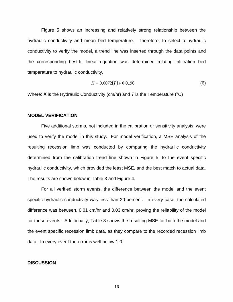
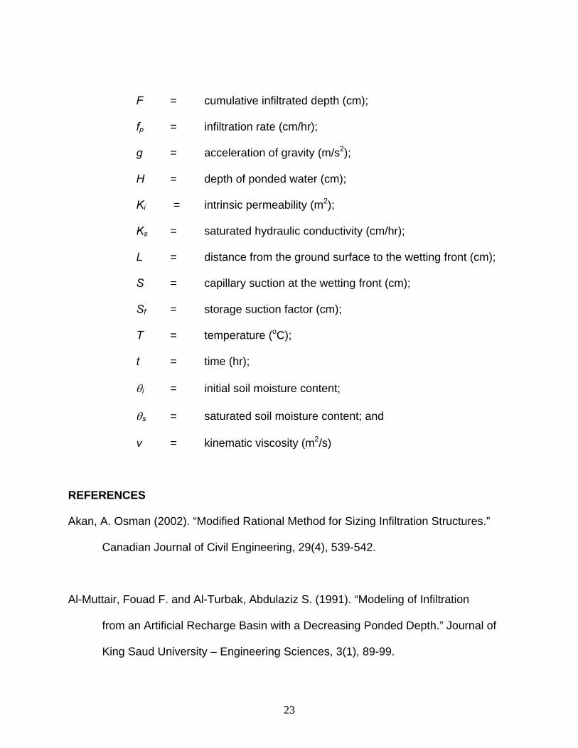