Temperature Effects on Productivity and FactorReallocation: Evidence from a Half Million Chinese

Manufacturing Plants∗

Peng Zhang† Junjie Zhang ‡ Olivier Deschenes § Kyle Meng ¶

August 24, 2016

Abstract

Understanding the relationship between temperature and economic growth is criti-cal to the design of optimal climate policies. A large body of literature has estimated anegative relationship between these factors using aggregated data. However, the micro-mechanism behind this relationship remains unknown; thus, its usefulness in shapingadaptation policies is limited. By applying detailed firm-level production data derivedfrom nearly two million observations of the Chinese manufacturing sector in the pe-riod of 1998-2007, this paper documents the relationship between daily temperatureand four components in a standard Cobb-Douglas production function: output, totalfactor productivity (TFP), labor, and capital inputs. We detect an inverted U-shapedrelationship between daily temperature and TFP; by contrast, the effects of tempera-ture on labor and capital inputs are limited. Moreover, the response function betweendaily temperature and output is almost identical to that between temperature andTFP, thereby suggesting that the reduction in TFP in response to high temperaturesis the primary driver behind output losses. In addition, temperature affects both la-bor and capital productivity. A medium-run climate prediction indicates that climatechange will reduce TFP by 4.18%, and result in output losses of 5.71%. This loss cor-responds to CNY 208.32 billion (USD 32.57 billion) in 2013 values. Given that TFP is

∗We thank Chris Costello, Soloman Hsiang, Charlie Kolstad, Peter Kuhn, Mushfiq Mobarak, PaulinaOliva, and Chris Severen for their comments and suggestions. This paper also benefits from seminar par-ticipants at UCSB, Shanghai Jiaotong University, Wuhan University, Renmin University of China, and theHong Kong Polytechnic University. Any remaining errors are our own.†School of Accounting and Finance; M705c Li Ka Shing Tower; The Hong Kong Polytechnic University;

Hong Hum, Kowloon, Hong Kong, peng.af.zhang@polyu.edu.hk‡School of Global Policy and Strategy, University of California, San Diego. 9500 Gilman Drive #0519,

La Jolla, CA 92093-0519. Tel: (858) 822-5733. Fax: (858) 534-3939, junjiezhang@ucsd.edu§Department of Economics; 2127 North Hall; University of California, Santa Barbara; Santa Barbara,

CA 93106, IZA and NBER, olivier@econ.ucsb.edu¶Bren School of Environmental Science and Management, and Department of Economics; 4416 Bren Hall;

University of California, Santa Barbara; Santa Barbara, CA 93106, and NBER kmeng@bren.ucsb.edu

invariant to the intensity of use of labor and capital inputs and reflects both labor andcapital productivity, the Chinese manufacturing industry is unlikely to avoid climatedamages simply by implementing factor allocation. Thus, new innovations that expandthe technology frontier for all inputs should be developed to offset weather-driven TFPlosses if other adaptation strategies are infeasible.

Keywords: Climate Change, TFP, Manufacturing, China

JEL Classification Codes: Q54, Q56, L60, O14, O44

2

1 Introduction

Understanding the effect of temperature on economic activity is critical to the design of

optimal climate policies (Dell et al., 2012). A growing body of literature has estimated the

historical effects of temperature on economic growth using reduced-form statistical meth-

ods (e.g., see Nordhaus and Yang (1996); Hsiang (2010); Dell et al. (2012); Burke et al.

(Forthcoming)), and strong negative effects have been detected in various parts of the world.

However, most of these studies are based on aggregated economic data; therefore, the spe-

cific micro-mechanism behind this relationship remains unknown. The usefulness of these

works is thus limited in terms of informing climate adaptation policies. In particular, the

sector whose losses are most responsible for GDP losses is unclear. Furthermore, whether or

not temperature affects output primarily through costly factor reallocation or productivity

losses remains unknown.

This paper fills this research gap in two ways. First, prior studies that use micro data

primarily examined productivity in the agricultural sector (e.g., see Mendelsohn et al. (1994);

Schlenker et al. (2005, 2006); Deschenes and Greenstone (2007); Schlenker and Roberts

(2009)). However, focusing solely on the agricultural sector cannot fully explain GDP losses

given the small share of agricultural output in many national economies. For example,

agriculture accounts for only 1% and 10% of the GDPs of the U.S. and of China, respectively;

by contrast, the manufacturing sector constitutes 12% and 32% of these GDPs (U.S. Bureau

of Economic Analysis, 2013; China Statistical Yearbook, 2014). Therefore, this paper selects

the Chinese manufacturing sector as the empirical setting because of its significance to

the Chinese economy. Furthermore, this sector comprises 12% of global exports (World

Bank, 2013a); thus, the output losses can have global general equilibrium consequences. In

addition, China is the world’s largest carbon dioxide (CO2) emitter (U.S. Energy Information

Administration, 2012); hence, the potential climate damages to the Chinese manufacturing

sector may motivate this country to develop more aggressive carbon reduction policies, which

is critical to mitigating global climate change.

1

Second, this paper documents the relationship between temperature and the four com-

ponents in a standard Cobb-Douglas production function: output, total factor productivity

(TFP), labor, and capital inputs, using detailed firm-level production data from nearly two

million observations in the manufacturing sector in China from 1998 to 2007. The primary

focus is TFP, which combines both labor and capital productivity and is invariant to the

intensity of use of labor and capital inputs (Syverson, 2011). TFP has been employed to

measure technology progress and is essential to economic growth (Aghion and Durlauf, 2005).

While recent works have investigated labor productivity in Indian manufacturing (Adhvaryu

et al., 2014; Somanathan et al., 2014), no study to date has jointly examined productivity

and factor allocation effects of temperature.

To identify the causal effects of temperature on TFP and other variables, we employ

year-to-year variation in a firm’s exposure to the distribution of daily temperatures, mod-

eled as 10-degree Fahrenheit (F) bins (Deschenes and Greenstone, 2011). We find an inverted

U-shaped relationship between daily temperature and TFP. The negative effect of extreme

high temperatures, above 90◦F, is particularly large in magnitude. In our preferred spec-

ification, one more day with temperatures above 90◦F decreases TFP by 0.56%, relative

to temperatures between 50-60◦F. Importantly, we find that the response function between

daily temperature and output is almost identical to that of TFP. By contrast, the effects on

labor and capital inputs are limited. This implies that the reduction in TFP in response to

high temperatures is the primary channel through which temperature affects manufacturing

output.

Given that TFP combines both labor and capital productivity, disentangling the effects

separately is important. Previous studies have largely focused on labor productivity (e.g.,

see Adhvaryu et al. (2014); Somanathan et al. (2014)), and ignored capital productivity.

High temperatures could cause discomfort, fatigue, and cognitive impairment on workers,

and reduce labor productivity. In addition, such temperatures could also affect machine

performance and lower capital productivity. Although one cannot explicitly disentangle TFP

2

as labor and capital productivity in a Cobb-Douglas production function, we can examine

differential TFP effects for labor- or capital-intensive firms. Various specifications suggest

that high temperatures affect both labor and capital productivity.

Firms are required to provide some protection for workers, such as hydration, air con-

ditioning, and subsidies during extremely hot days in China.1 Given the relative rigidity

of labor regulations in state-owned firms compared with those of private firms, one may

expect effects of high temperatures on TFP to differ based on firm ownership. Our empirical

results support this argument. We find that the effects of high temperatures on TFP for

state-owned firms are slightly positive. On the contrary, TFP in private firms exhibits larger

negative response to high temperatures. This implies that labor regulations could play an

important role in mitigating the negative effects of high temperatures.

Lastly, using the estimated coefficients of climatic variables on output and TFP, we

predict a medium-run climate effect on output and TFP. Compared with the periods from

1998-2007, climate change is likely to reduce output by 5.71% by 2020-2049, which is mainly

caused by the reduction in TFP. This is equivalent to CNY 208.32 billion (USD 32.57 billion)

losses in 2013 values. Given that China is the world’s largest exporter and manufacturing

goods comprise 94% of total exports (World Bank, 2013a), the output losses could have

global general equilibrium consequences via trade.

This paper contributes to the existing literature in three aspects. First, to our best

knowledge, this paper is the first to present a possible micro-mechanism for considerable

studies that focus on temperature and economic growth (Nordhaus and Yang, 1996; Hsiang,

2010; Dell et al., 2012; Burke et al., Forthcoming). We find that a 1◦F (1◦ Celsius (C))

increase in annual mean temperature reduces China’s GDP by 0.92% (1.66%). This finding

is consistent with Hsiang (2010) and Dell et al. (2012); they find that a 1◦F (1◦C) increase in

annual mean temperature leads to 1.39% (2.5%) and 0.56% (1.0%) GDP reduction in other

developing countries. Our results suggest that the reduction of TFP in the manufacturing

1http://www.chinasafety.gov.cn/newpage/Contents/Channel_20697/2012/0704/173399/content_

173399.htm.

3

sector as a response to high temperatures is primarily responsible for the negative relationship

between temperature and economic growth.

Second, this paper provides the first study that documents the relationship between

daily temperature and TFP. Unlike single-factor productivity which heavily depends on the

intensity of use of the excluded factor, TFP is invariant to labor and capital inputs, and thus

is more likely to capture the true productivity. Furthermore, high temperatures affect both

labor and capital productivity, the latter of which has been ignored in the literature.

Third, a large body of literature in macroeconomics, industrial organization, labor, and

trade seeks to understand the determinants of productivity (Syverson, 2011). This paper

provides a new channel: weather, or specifically, temperature. High temperatures, especially

above 90◦F, have a significantly negative effect on TFP. Given the typical fluctuation of

temperature across space and over time, this exogenous variation could further cause TFP

dispersion across firms.

The results of this paper have considerable policy implications. If high temperatures

only affect labor productivity, then manufacturing could adapt to climate change by simply

shifting from being labor-intensive to being capital-intensive. However, because TFP reflects

both labor and capital productivity, and is invariant to the intensity of inputs, temperature

could induce shifts in isoquants rather than along isoquants. Therefore, Chinese manufac-

turing is less likely to avoid damages under climate change simply by reallocating labor and

capital inputs. Indeed, new innovations that expand the technology frontier for all inputs

need to occur to offset weather-driven TFP losses if other adaptation strategies are infeasible.

In addition, the empirical setting is Chinese manufacturing, which is critical for the

Chinese economy. The new findings of potential damages on the manufacturing sector could

be incorporated in the cost-benefit analysis in designing climate policies, and motivate China

to aggressively act on reducing carbon emissions with self interest in mind. As the world’s

largest emitter of CO2 (U.S. Energy Information Administration, 2012), China’s effort is

critical in mitigating global climate change.

4

Finally, transitioning from agriculture to manufacturing is recognized as a feasible way to

aid Sub-Saharan Africa in adapting to climate change (Henderson et al., 2015). Nonetheless,

climate change may also impact the African manufacturing industry given the significant

climate damages to the Chinese manufacturing sector described in this paper. Therefore,

the estimates in this research need to be generalized to other countries to improve the support

for adaptation policy design.

The rest of the paper is organized as follows. Section 2 presents a simple conceptual

framework that helps the empirical analysis. Section 3 describes data sources and summary

statistics. Section 4 presents the empirical strategy and the identification. Section 5 describes

the results and interpretation. Section 6 predicts the impacts of climate change on output

and TFP. Section 7 offers economic and policy implications and Section 8 concludes.

2 Background and Conceptual Framework

This section provides a simple conceptual framework and the channels that how temperature

might affect the four components in a production function: output, TFP, labor, and capital

inputs.

Consider a standard Cobb-Douglas production function for an industry

Y (T ) = A(T )L(T )αK(T )β. (1)

Here, Y denotes output and L and K denote labor and capital, respectively. In practice,

output is measured by value added; therefore, material input is excluded from the production

function. The Hicks-neutral efficiency level, or TFP, is represented by A. Output elasticities

of labor and capital are measured by α and β. Temperature, denoted as T , could affect

output through productivity and inputs.

5

Taking natural logs of the above equation leads to the following function

y(T ) = a(T ) + αl(T ) + βk(T ), (2)

where lowercase symbols represent natural logs of variables. It is worth noting that TFP is

a weighted average of labor and capital productivity. To see this, consider a Cobb-Douglas

production function that distinguishes labor and capital productivity

Y (T ) = (AL(T )L(T ))α(AK(T )K(T ))β, (3)

where AL and AK denote the labor and capital productivity, respectively. Taking natural

logs of the above equation results in the following equation

y(T ) = αaL(T ) + βaK(T ) + αl(T ) + βk(T ). (4)

Comparing the above equation with Equation (2), one can obtain

a(T ) = αaL(T ) + βaK(T ), (5)

which suggests that TFP is a weighted average of labor and capital productivity, where

the weights are output elasticities of labor and capital inputs. However, in practice, one

cannot estimate Equation (4) because of two unknowns (aL and aK) within one equation.

It is common practice for labor productivity to be measured by output per worker, i.e.,

Y/L. Similarly, capital productivity is sometimes measured by output per capital, or Y/K.

However, this single-factor productivity measurement heavily depends on the intensity of

excluded factor, and may not reflect the true productivity (Syverson, 2011). For example,

two firms with the same technology could have different labor productivity levels because

one happens to use more capital.2

2To see this, consider two firms within the same industry that share the following Cobb-Douglas produc-

6

Temperature could affect TFP through labor productivity. High temperatures not only

physiologically affect human body and cause discomfort and fatigue, it may also affect cogni-

tion function and psychomotor ability (Hancock et al., 2007; Graff Zivin et al., 2015). Several

studies have estimated the impacts of temperature on labor productivity using either lab ex-

periments (e.g., see Niemela et al. (2002); Seppanen et al. (2003, 2006)) or reduced-form

statistical methods (e.g., see Graff Zivin and Neidell (2014), Adhvaryu et al. (2014), and

Somanathan et al. (2014).)3

Temperature also affects TFP through capital productivity. Evidence shows that high

temperatures could dramatically impact machine performance. For example, lubricant helps

reduce friction between surfaces in machines. It also helps transmit forces and transport for-

eign particles, and has been regarded as one of the key factors for machine performance (Ku,

1976). High temperatures could negatively affect lubricant efficiency by influencing their

viscosity and pour point (Mortier et al., 1992). Moreover, high temperatures could expand

most materials used in manufacturing by altering their coefficients of thermal expansion

(Collins, 1963), and further increase gaging error in the manufacturing process. Computers

play a major role in modern manufacturing. Excessive heat could lower the electrical resis-

tance of objects and increase the current, which may slow down the processing performance

of a computer (Lilja, 2000). It is noteworthy that the evidence presented above is mainly

suggestive. To date, no rigorous study has focused on temperature and capital productivity.

Furthermore, temperature could affect labor inputs. Given the negative effects of high

temperatures, workers may reduce working hours or even be absent from work. Several

studies estimate the effects of temperature on labor supply (e.g., see Graff Zivin and Neidell

(2014) and Somanathan et al. (2014)).4 Temperature could also affect capital stock. For

tion function Y = AL1/2K1/2. The following values are assigned to firm 1: A1 = 1, L1 = 1, K1 = 1. Onecan obtain Y1 = 1, and labor productivity Y1/L1 = 1. Similarly, the following values are assigned to firm 2:A2 = 1, L2 = 1, K2 = 4. One can obtain Y2 = 2, and labor productivity Y2/L2 = 2. Both firms have thesame TFP levels, but the second firm exhibits higher labor productivity than the first because the secondfirm uses more capital.

3See a detailed review in Dell et al. (2014).4See Heal and Park (2013) for a conceptual framework regarding the effects of temperature on labor

supply.

7

example, high temperatures may abrade machines and lead to faster capital depreciation.

Given the possible effect of temperatures on all the three inputs in the production function,

naturally, temperatures may also affect output.

3 Data

3.1 Firm Data

Firm-level data come from the annual surveys conducted by the National Bureau of Statistics

(NBS) in China. This survey covers all industrial firms, either state-owned or non-state with

sales over CNY 5 million (USD 0.8 million) from 1998 to 2007 (hereafter referred to as the

“above-scale” industrial firms).5 The industrial sectors here include mining, manufacturing,

and public utilities, in which manufacturing composes 93.52% of the total observations.

Given that manufacturing composes the largest share of the industrial sector, we use the

terms manufacturing sector and industrial sector interchangeably throughout the paper.6

We address several empirical issues. First, each firm has a unique numerical ID. However,

firms may change their IDs because of restructuring, acquisition, or merging. We use the

matching algorithm provided in Brandt et al. (2012) to match firms over time.7

Second, the data contain outliers. We take standard procedures in the literature that have

used this data (Cai and Liu, 2009; Brandt et al., 2012; Yu, 2014). First, we drop observations

with missing or negative values for value added, employment, and fixed capital stock. Second,

we drop observations with employment less than 10, because these small firms may not have a

reliable accounting system. Third, we drop observations that apparently violate accounting

principles: liquid assets, fixed assets, or net fixed assets larger than total assets; current

5According to the census of manufacturing firms conducted by NBS in 2004, the above-scale firms con-tribute more than 91% of the total output. Therefore, the sample used in this study is representative of theChinese industrial sector.

6The main results are robust when we focus on manufacturing sector only.7The basic idea involves first matching firms according to their IDs and then linking them using infor-

mation on firms’ names, legal persons, industry codes, and others.

8

depreciation larger than accumulative depreciation. Finally, we drop observations with the

values of key variables outside the range of 0.5 to 99.5 percentile. Overall, approximately

10% of observations are dropped.8

Third, in the data, each firm is classified into a four-digit Chinese Industry Classification

(CIC) code, which is similar to the U.S. Standard Industrial Classification (SIC) code. How-

ever, in 2003, the NBS adopted a new CIC system. Several sectors were merged whereas new

sectors were created. Following Brandt et al. (2012), we revise codes before 2003 to make

them consistent with codes after 2003. Overall, the sample contains 39 two-digit sectors,

193 three-digit sectors, and 497 four-digit sectors.

3.2 Measuring Firm-level TFP

Several approaches are used to estimate firm-level TFP. These methods are debated in the

literature and each requires particular assumptions (Van Biesebroeck, 2007). Fortunately,

all these measurements are sufficiently robust to empirical specifications (Syverson, 2011).

In this paper, we use the Olley-Pakes estimator (Olley and Pakes, 1996) to estimate TFP.

The index number approach (Syverson, 2011) is used for a robustness check.

Consider a standard linearized Cobb-Douglas production function

yit = βllit + βkkit + uit, (6)

where yit is the log output for firm i in year t; lit and kit are log values of labor and capital

inputs, respectively; βl and βk are output elasticities of labor and capital that need to be

estimated; uit is the error term. Hence, the log TFP is the residual uit = yit − βllit − βkkit.

The OLS estimates of Equation (6) may be biased because of simultaneity and sample

selection. Simultaneity bias arises because firms can observe productivity and then make

decisions on labor and capital inputs. Thus, lit and kit are likely to be correlated with uit.

8Generally, the results are robust to those outliers.

9

Furthermore, firms with lower productivity may be more likely to exit from the market, and

thus result in selection bias.

Olley and Pakes (1996) propose an estimator that controls for the simultaneity and

selection biases. The basic idea is to use investment to proxy for unobserved productivity

shocks, and use a firm’s survival probability to correct for selection bias. The Olley-Pakes

estimator is widely used in the literature,9 and thus serves as the baseline measurement of

TFP in this paper.10

The Olley-Pakes estimator requires parametric estimation of the production function.

The index number approach, however, is free of the parametric assumption. Indeed, we

simply use the share of wage bill in value added to measure output elasticity of labor input

βl, and use 1 − βl to measure output elasticity of capital input βk.11 The index number

approach requires the assumptions of perfect competition and constant returns to scale.

These assumptions seem strong in our empirical setting, and thus the index number approach

will serve as a robustness check.

In practice, yit is measured by value added; lit is measured by employment, and kit, is

measured by fixed capital stock. Investment is constructed using the perpetual inventory

method. All monetary variables are deflated using the industry-level price indexes following

Brandt et al. (2012). Furthermore, Equation (6) is estimated separately for each two-digit

industry.

9For example, see Pavcnik (2002); Javorcik (2004); Amiti and Konings (2007); Brandt et al. (2012).10Levinsohn and Petrin (2003) argue that the use of investment to control for unobserved productivity

shocks may be inappropriate in certain empirical settings because investment must be strictly positive in theOlley-Pakes estimator. Nonetheless, this issue is minor in our empirical setting. Given the rapid developmentin China, few observations indicate negative or zero investment. Furthermore, the Levinsohn-Petrin estimatordoes not control for selection bias; thus, we prefer the Olley-Pakes estimator. Nonetheless, the results remainrobust when we use the Levinsohn-Petrin estimator.

11It would be ideal to use capital share to measure βk; however, data on capital rental rate is not available.

10

3.3 Weather Data

The weather data are drawn from the National Climatic Data Center (NCDC) at the Na-

tional Oceanic and Atmospheric Administration (NOAA).12 NCDC reports global station-

level weather data at three-hour intervals from 1901-2015. We extract the data covering

China from 1998-2007.13 Auffhammer et al. (2013) suggest the importance of keeping a

continuous weather record when using daily weather data because missing values may con-

taminate the estimates. As such, we choose stations with valid weather records for 364 days

in a year and fill in the rest of the missing values using the average between the preceding

and subsequent days.14

The weather data contain major climatic variables, including temperature, precipitation,

dew point temperature, visibility, and wind speed. Relative humidity is not reported in

the NCDC data, but is constructed from the standard meteorological formula provided by

NOAA using temperature and dew point temperature.15 Zhang et al. (2015) demonstrate the

importance of additional climatic variables other than temperature and precipitation. Thus,

we include temperature, precipitation, relative humidity, and wind speed in our empirical

specifications. We use the daily mean values of each climatic variable calculated as the

averages of the three-hour values as the main measurement of weather, except precipitation

which is constructed as daily total values. In addition, we use visibility as a proxy for

air pollution (Ghanem and Zhang, 2014). Air pollution is typically correlated with climatic

variables (Jayamurugan et al., 2013) and affects productivity as well (Graff Zivin and Neidell,

2012). Therefore, omitting air pollution may induce the omitted-variable bias.

The variable of interest in this analysis is temperature. Temperature may have a joint

impact with humidity on productivity. For example, when temperature is high, the human

12The data can be downloaded from the website ftp://ftp.ncdc.noaa.gov/pub/data/noaa/.13Approximately 400 stations cover China. Refer to Figure B.10 for a detailed distribution of weather

stations.14We do not choose stations that are operational for all 365 days because all stations are missing one day’s

weather records for the years 1999 and 2007.15A detailed explanation is provided in the online appendix.

11

body may cool itself down through perspiration. However, this process is hard in a more hu-

mid environment. Consequently, we also use the heat index to measure the joint influence of

temperature and humidity on productivity as a robustness check. Heat index is constructed

following the standard formula provided by the NOAA.16

3.4 Climate Prediction Data

The climate prediction data are drawn from the Hadley Centre, one of the world’s leading

institutes in climate prediction. We focus on the Hadley Centre’s Third Coupled Ocean-

Atmosphere General Circulation Model (HadCM3), which has been commonly used in the

literature (Schlenker et al., 2006; Schlenker and Roberts, 2009; Deschenes and Greenstone,

2011).17 HadCM3 reports global grid-level daily temperature, precipitation, relative humid-

ity, and wind speed from 1990 to 2099. The grid points are separated by 2.5◦ latitude and

3.75◦ longitude. We focus on the “business-as-usual” (A1FI) scenario and choose the years

from 2020-2049, a medium-run period. We do not choose a long period such as 2070-2099

because technology could be much advanced at that time and may be insensitive to high

temperatures. Given that technology advancement may still be limited in a short time frame,

the climate prediction could be more realistic and meaningful.

Systematic model errors may exist between HadCM3 and NOAA, which may lead the

predictions to be inaccurate.18 Therefore, we implement the error-corrected method proposed

by Deschenes and Greenstone (2011). First, we calculate the difference in weather data from

1998-2007 between NOAA and HadCM3. We then add the difference to the prediction by

HadCM3, to correct for systematic model errors.

16The online appendix presents a detailed explanation of heat index calculation.17The data can be downloaded at http://browse.ceda.ac.uk/browse/badc/hadcm3. We do not use

other climatic models because such models typically report only temperature and precipitation data.18The systematic model errors are indeed severe in our sample. The average temperature for the period

of 1998-2007 in China is 54◦F according to NOAA but only 49◦F as per HadCM3.

12

3.5 Matching Firm and Weather Data

Firm-level data and station-level weather data are merged by county and year.19 First, we

transform weather data from station level to county level using the inverse-distance weighting

method, which is widely used in the literature (Mendelsohn et al., 1994; Deschenes and

Greenstone, 2007, 2011). The basic algorithm of this approach is to first choose a circle with

a 200 km radius for each county’s centroid. Then, the weighted average of weather data for

each station within the circle is assigned to that county, where the weights are the inverse

of the distance between each station and the county’s centroid. Finally, we assign each firm

with the weather data in that county where the firm is located.20 A similar way is used

to transform climate prediction data from the grid level to the county level.21 The merged

data leave an unbalanced panel from 1998-2007 for 511,352 firms with nearly two million

observations.

Table 1 presents the summary statistics of the merged data. The data cover all state-

owned firms and non-state firms with sales over CNY 5 million (USD 0.8 million) from 1998

to 2007. The industry sectors include mining (3.81%), manufacturing (93.52%), and utilities

(2.67%). Unit of observation is a firm-year. All monetary values are expressed in constant

1998 CNY.

Output is measured by valued added, which is the difference between total output and

intermediate input. From 1998 to 2007, the annual average output is approximately CNY

12 million (USD 2 million). To demonstrate the regional heterogeneity in output, Figure 1

depicts the average annual aggregate output in each county during 1998-2007. Generally,

aggregate output is the largest in the south and the east, suggesting that manufacturing

firms are mostly located in those regions.

19We do not observe the specific latitude and longitude of firms. Indeed, county is the smallest geographicunit representing a firm’s geographic location.

20The firm data are presented at firm level and not plant level; therefore, firms with multiple brancheslocated in different regions may be assigned erroneous weather data. Nonetheless, more than 95% of firmsin the sample are single-plant firms (Brandt et al., 2012); thus, this issue should exert little effect on theestimates.

21A 300 km radius is assigned to ensure that each county has a valid observation for the period of 2020-2049.

13

TFP is measured by the Solow residual in a Cobb-Douglas production function using

the Olley-Pakes estimator (Olley and Pakes, 1996). The average log TFP is 2.90, but varies

from -3.56 to 8.84, suggesting a large dispersion of TFP across firms exists. The dispersion

of TFP could be caused by many factors, and temperature may be an important one. Labor

is measured by employment, with an average of 200 people. Capital is measured by the fixed

capital stock. The average is CNY 15 million (USD 2.35 million).

Temperature, wind speed, visibility, and relative humidity are calculated as annual mean

value using daily observations. Precipitation is calculated as annual cumulative value using

daily observations. Past climate is calculated during the period 1998-2007 from NOAA,

whereas the future climate is calculated over the period 2020-2049 from HadCM3 with error

correction.22 The average temperature during 1998-2007 in the sample is 61.54◦F (16.41◦C).23

In general, temperature is expected to increase by 2◦F (1.11◦C), whereas precipitation is

expected to increase by 3 inches under climate change in China. Relative humidity and wind

speed are relatively unchanged when comparing 2020-2049 to 1998-2007, which is only a

medium-run prediction. In a long-run prediction (2070-2099), climate change is expected to

significantly increase temperature, precipitation, relative humidity, and wind speed in China

(Zhang et al., 2015).

4 Empirical Strategy

4.1 Measuring the Effect of Daily Temperature on Annual TFP

The TFP measurement is constructed at annual level because output and input are only

observed annually. To measure the effects of daily temperatures on annual TFP, We employ

a semi-parametric method, the so called bin approach, which has been widely used in the

22HadCM3 A1FI scenario does not predict for visibility.23Firm-average temperature is higher than county-average temperature because 67% of firms are located

in the south, which is typically warmer than the north. Similarly, precipitation and relative humidity levelsare also higher in this area.

14

literature (Schlenker and Roberts, 2009; Deschenes and Greenstone, 2011; Graff Zivin and

Neidell, 2014; Deryugina and Hsiang, 2014). The basic idea of the bin approach is to divide

daily temperature into small bins and then count the number of days falling into each bin.

This semi-parametric approach allows flexible model specifications of measuring nonlinear

effects of temperature and also preserves daily variations in temperature.

To develop the intuition of measuring annual TFP using daily temperatures, we present

a thought experiment motivated by Deryugina and Hsiang (2014). Suppose that only two

days are in a year, and each day could be either hot or normal. Considering the possible

effect of high temperatures on productivity, a firm could only produce one product given a

certain amount of labor and capital inputs on a hot day, but could produce two products

given the same inputs on a normal day. In addition, we assume only two years: year t and

year t+ 1, each with only two days. In year t, one day is normal and other other day is hot.

In year t + 1, both days are hot. Suppose that a typical firm uses the same inputs in both

years,24 then, it will produce 3 goods in year t and 2 goods in year t+1. Thus, one more hot

day decreases productivity by 1, or 33%.

Furthermore, using annual TFP measurement could capture adaptations of firms in re-

sponse to high temperatures within a year. For example, firms may adjust their production

period from hot to cool days. This adjustment behavior will be absorbed by annual TFP

measurement. Thus, our estimates are more likely to have considered within-year adaptation.

In practice, we divide daily temperature, measured in ◦F, into ten bins. Temperatures

below 10◦F are defined as the 1st bin, and temperatures between 10-20◦F are defined as the

2nd bin, etc. Finally, temperatures above 90◦F are defined as the 10th bin, which represents

extremely high temperatures.

Figure 2 plots average annual distribution of daily temperatures across different bins. The

blue bar “1998-2007” indicates past climate, i.e., during the period 1998-2007, whereas the

red bar “2020-2049” denotes future climate (2020-2049). The height of each bin represents

24Temperature may also affect labor and capital inputs, but TFP is invariant to inputs.

15

the average number of days falling into that bin’s range per year. For example, the height

of the bin above 90◦F is approximately 2, which indicates that on average, there are two

days per year with temperature over 90◦F. As expected, climate change is likely to shift the

distribution of temperature to the right, and lead to more extremely hot days.

It is important to know that the changes in temperature distribution are not uniform

across China. To demonstrate the regional heterogeneity in climate change, Figure 3 depicts

the changes in days with temperatures above 90◦F for each county under a medium-run

climate prediction. Each observation records the difference in days with temperatures above

90◦F between the periods of 2020-2049 and 1998-2007. The east and the south will generally

experience more extremely hot days.

Other than temperature, this paper also includes precipitation, relative humidity, visibil-

ity, and wind speed. For simplicity, those variables are constructed as annual means, except

precipitation calculated as annual cumulative value. We also include a quadratic for those

variables to account for nonlinearity.25

4.2 Regression Model and the Identification

To explore the effects of temperature on the four components of the Cobb-Douglas production

function (see Equation (2)), especially TFP, we estimate the following fixed-effect regression

models

ln yit = β′Tempit + δ′wit + θ′zit + αi + εit, (7)

where i indexes a firm, and t references a year.

In this form, yit denotes the four components in Equation (2): output, TFP, labor, and

capital inputs. All these variables are represented in logarithms, and thus, our estimates

can be illustrated as semi-elasticities. The variable of interest, Tempit, contains a vector

25Readers interested in the changes in the distribution of precipitation, relative humidity, and wind speedunder climate change in China can refer to Zhang et al. (2015).

16

of temperature bins [Tbinit1, · · · ,Tbinit10], in which Tbinitj denotes the number of days

falling into the jth temperature bin for firm i in year t. Other climatic variables, including

precipitation, relative humidity, wind speed, and visibility, are included in vector wit. The

vector zit contains a set of fixed effects, including year-by-region fixed effects and year-by-two-

digit-sector fixed effects.26 Year-by-region fixed effects control for shocks common to each

geographic region in a year, such as climate trends, technology, and policy shocks within

each geographic region. Year-by-two-digit-sector fixed effects control for shocks common to

each two-digit sector in a given year, such as input and output price shocks and technology

shocks within each two-digit industry. We use firm fixed effects αi to control for firm-specific

time invariant characteristics, such as geographic locations. Lastly, εit is an unobservable

error term.

Several noteworthy econometric details exist. First, it is likely that the error terms

are both spatial and serial correlated. Thus, standard errors are clustered in two ways:

within firm and within county-year (Cameron et al., 2011). The former will control for the

serial correlation along time within each firm, whereas the latter will account for the spatial

correlation across firms within each county in a given year.

Second, because each day is assigned into different bins, the sum of all bins∑

j Tbinitj

is exactly equal to 365.27 To avoid multicollinearity, we normalize the coefficient for the 50-

60◦F bin to zero. Thus, all estimates of other temperature bins are impacts relative to the

reference group 50-60◦F. We choose 50-60◦F as the reference group because it is in the middle

of temperature ranges and thus makes the illustration of results more intuitive. However,

our conclusion does not hinge on the choice of this reference group.

The coefficient of central interest is the estimate for each temperature bin. Considering

26We do not use more disaggregated fixed effects such as year-by-four-digit-sector fixed effects and year-by-province fixed effects because of the computational constraints (Greenstone et al., 2012). Furthermore,year-by-province fixed effects are likely to absorb a significant share of exogenous variations in weather giventhat weather is typically homogeneous within a province (Fisher et al., 2012). Region classification data areshown in Table B.8.

27In 2000 and 2004, the sum of all days is equal to 366. We drop February 29th to ensure that the sum ofall days is constant for the period of 1998-2007.

17

that the dependent variables are all measured in logarithms, temperature effect βj measures

the percentage change, or the semi-elascticities in the four components of the production

function for a firm if it has one more day falling into the jth temperature bin, relative to

the 50-60◦F bin. The marginal effects of each temperature bin could be used to evaluate the

marginal cost of increasing temperatures induced by climate change.

The identification of the key parameter relies on year-to-year weather fluctuations within

firms over time. Formally, for the jth temperature bin, the identification assumption is

E [Tbinitjεit|Tbinit,−j, wit, zit, αi] = 0. (8)

As suggested by Deschenes and Greenstone (2007), weather fluctuations are generally ran-

dom and less predictable. Thus, we can reasonably assume that the jth temperature bin is

orthogonal to the error term, conditional on other controls. Furthermore, Zhang et al. (2015)

argue that climatic variables are generally inter-correlated. As such, omitting other climatic

variables apart from temperature and precipitation may bias the estimates. This study in-

cludes a rich set of climatic variables other than temperature and precipitation, including

relative humidity, wind speed, and visibility. This will further solidify the identification

assumption.

5 Results

5.1 Baseline Results

This section presents the baseline regression results estimated using Equation (7). To vi-

sualize the effects, Figure 4 plots the response function between daily temperature and the

four components in a Cobb-Douglas production function: output, TFP, labor, and capital

inputs. Specifically, it plots the point estimates as well as the 95% confidence intervals for

each temperature bin estimated in four regressions. Bin 50-60◦F is normalized to zero. As

18

such, other estimates are relative to the reference group.

Panel A in Figure 4 depicts the response function between daily temperatures and log

output. In general, we find an inverted U-shaped relationship between temperature and

output.28 The shape is relatively smooth and precisely estimated. The negative effects of

extremely high temperatures (above 90◦F) are both economically and statistically significant.

The point estimate suggests that one more day with temperatures larger than 90◦F decreases

output by 0.45%, relative to the impact of temperature bin 50-60◦F. In the sample, the

average annual aggregate output for all firms is CNY 2.69 trillion (USD 0.43 trillion) in 1998

values. This suggests that, one more day with temperatures above 90◦F decreases output

by CNY 12.11 billion (USD 1.89 billion), relative to the impact of temperature bin 50-60◦F.

Given that climate change will shift the distribution of temperature to the right and induce

more extreme hot days (Figure 2), a substantial economic loss in the manufacturing sector

in China under climate change may be expected.29

Given that temperatures, particularly high temperatures, have a significantly negative

effect on output, the mechanism, i.e., which component leads to the reduction in output,

may be the next concern. Thus, panels B, C, and D plot the response function between daily

temperature and TFP, labor, and capital inputs.

Several findings can be made from these figures. First, the response function between

daily temperature and TFP is very close to daily temperature and output. An inverted

U-shaped relationship is observed in both panels A and B. The magnitudes of the point

estimates are close. However, the gradient depicted in panel B is slightly steeper than

presented in panel A in the high-temperature ranges. For example, one more day with

temperature higher than 90◦F reduces output by only 0.45% but lowers TFP by 0.56%.

28Surprisingly, bin 30-40◦F, which is a relatively cold range, reports the largest point estimate and isstatistically significant. This outcome is because TFP combines both labor and capital productivity; while30-40◦F is cold for human behaviors, this range may be suitable for machine performance.

29Extremely cold days, such as those with temperatures below 10◦F, are reduced under climate change.This occurrence may benefit the manufacturing sector. However, the losses induced by the increased numberof extremely hot days should dominate these gains because the point estimate of extremely hot days is muchlarger than that of extremely cold days.

19

The effects of daily temperature on labor (panel C) and capital (panel D) do not take

a particular shape. Furthermore, the estimates of most temperature bins are statistically

insignificant; however, a slight increase is observed in the highest temperature range depicted

in panel C, and the effect is statistically significant at conventional levels. This outcome sug-

gests that firms may employ additional labor in response to high temperatures, to partially

compensate the output losses driven by TFP losses. This result explains why the TFP losses

are slightly greater than the output losses in response to high temperatures. By contrast,

the effect on capital is statistically insignificant because capital is generally unadjustable in

the short run.

Table 2 further presents the effects of daily temperatures on output and TFP using

various specifications. Due to space limitations, we only report the regression results of the

two highest temperature bins: 80-90◦F and above 90◦F. Furthermore, the F -statistic of the

null hypothesis, that the coefficients of all temperatures bins are jointly equal to zero, are

also reported.

In column (1a), we start with a simple specification of only firm fixed effects and year

fixed effects. Thus, the identification is from plausibly exogenous variations in weather

within firms over time after we adjusted nationwide shocks in a given year. These shocks

may include policy changes, technology progress, or price shocks of inputs and output that

are common to the country. However, some shocks may be region-specific. Thus, in column

(1b), we replace year fixed effects with year-by-region fixed effects, which control for any

common shocks for a specific geographic region in a given year.

In column (1c), we replace year fixed effects with year-by-two-digit-sector fixed effects to

control for shocks that are common to two-digit industries in a given year. These shocks may

include sector-specific price shocks of inputs and output. In addition, technology progress

within each industry are included in year-by-two-digit-sector fixed effects. Column (1d)

includes both year-by-region and year-by-two-digit-sector fixed effects, which will control for

common shocks within geographic regions and two-digit sectors.

20

Through columns (1a)-(1d), temperature bins are constructed using daily mean temper-

ature. In column (2a), temperature bins are constructed using daily maximum temperature

to capture the daily extremely hot effects that may be missed using daily mean temperature.

In column (2b), we construct temperature bins using daily heat index, which incorporates

the effects of both temperature and humidity.

TFP is estimated as the Solow residual in a Cobb-Douglas function using the Olley-

Pakes estimator (Olley and Pakes, 1996) through columns (1a) to (2b). In column (3), TFP

is estimated using the index number approach (Syverson, 2011) to verify the robustness of

different TFP measures. Temperature bins are constructed using daily mean temperature

and the model includes firm fixed effects, year-by-region fixed effects, and year-by-two-digit-

sector fixed effects.

The major conclusion that high temperatures have a significantly negative effect on both

output and TFP is robust across various specifications. The F -statistic for all temperature

bins are all statistically significant, suggesting that the effects of all temperature bins are

jointly different from zero.

Columns (1a) to (1d) test the robustness of fixed effects. In general, controlling for geo-

graphic shocks produces larger estimates. This is likely because manufacturing plants built

in hot regions may be equipped with heat-proof materials. When year-by-region fixed effects

are included, we are comparing firms within each geographic region; thus, this protection

measure was absorbed. Therefore, the model with year-by-region fixed effects produces larger

estimates. The estimates are relatively unchanged when including year-by-two-digit-sector

fixed effects. The most robust specification, column (1d), controls for both geographic and

industrial shocks. Thus, this specification will serve as the baseline in this paper.

Column (2a) tests the robustness of daily temperature measures, and produces the small-

est negative estimates. This is because when temperature bins are constructed using daily

maximum temperatures, above 90◦F are actually not particularly hot. Column (2b) incor-

porates the joint effects of temperature and humidity, and produces slightly smaller effects,

21

indicating that the effects of humidity may be limited. Column (3) tests the robustness

of TFP measures. The results suggest that our estimates are robust to alternative TFP

measures using the index number approach, though the magnitude is smaller.

In terms of climatic variables other than temperature, precipitation and wind speed

generally have a significantly negative impact on output and TFP; by contrast, the effects of

relative humidity and visibility are statistically insignificant. The results are listed in Table

B.9, which is provided in the online appendix.

5.2 Effects of Lagged Temperatures

The temperatures in previous years may have an effect on current economic outcomes (Dell

et al., 2012; Deryugina and Hsiang, 2014). For example, hot temperatures in the prior year

may reduce the output, and further reduce investment. This outcome may affect capital

accumulation, and reduce current output. Therefore, in this section, we include one-year

lagged temperature, measured in 10◦F bins, in the baseline regression model.30 Both current

and lagged temperatures are estimated simultaneously in one regression.

Figure 5 presents the effects of both current and lagged temperatures on output and

TFP. Panel A depicts the response function between current daily temperature and output,

whereas panel B depicts the response function between lagged daily temperature and output.

Panels C and D also depict the response function, but with the dependent variable as log

TFP.

Panels A and C show that the effects of current temperatures on both output and TFP

still remain as inverted-U shapes when we include lagged temperatures. The response func-

tion between current daily temperature and output and TFP are qualitatively almost the

same, with and without including lagged temperature. As shown in panels B and D, the

effects of lagged temperatures on output and TFP are not clear. Overall, the point estimates

30We do not include further lags because temperature is measured in 10 bins, and 2-year lags already resultin 30 dependent variables. Therefore, we are unlikely to generate adequate statistical power to identify theeffects of temperature on output and TFP.

22

are mostly noisy results, and do not exhibit any particular shapes. Thus, lagged tempera-

tures, especially lagged high temperatures, seem to have limited effects on both output and

TFP.31

5.3 Effects of Temperature on TFP Growth

Temperatures may not only affect the level of TFP, but also influence growth rate through

investments or institutions (Dell et al., 2012). To verify this hypothesis, Equation (7) is

estimated with the dependent variable as TFP growth rate. Given that the effects of tem-

perature on TFP growth rate may be time lagged, we include one-year lagged temperature

bins.

Figure 6 plots the response function between daily temperature and TFP growth rate.

Panel A is for current daily temperature, while panel B is for one-year lagged daily tempera-

ture. Surprisingly, we do not find an effect of either current or lagged temperatures on TFP

growth rate. In panel A, the response function is relatively flat. Although the temperature

range above 90◦F slightly dropped, it is statistically insignificant. Moreover, in panel B, most

estimates, particularly high temperature ranges, are statistically insignificant. Panels C and

D further depict the response function between daily temperature and log investment. We

do not find a significant effect of either current or lagged daily temperature on investment.

Most estimates are statistically insignificant and not well-estimated. This suggests that the

effects of temperatures are mostly significant on the level of TFP, instead of the growth rate.

5.4 Disentangling TFP into Labor and Capital Productivity

We have shown that the negative effects of temperature on TFP is the major force that

drives the reduction in output. Given that TFP is a weighted average of labor and capital

productivity, whether the negative effects primarily originate from labor productivity, capital

31In general, we do not detect the significant impacts of both current and lagged temperature on laborand capital inputs either.

23

productivity, or both, is a question of interest. Previous studies have predominantly focused

on labor productivity (e.g., see Adhvaryu et al. (2014); Somanathan et al. (2014)), while

ignoring capital productivity. Because one cannot estimate labor and capital productivity

separately in a Cobb-Douglas production, we have to implicitly test the hypothesis that

the negative effects of TFP are mostly from labor productivity. The intuition is as follows.

We recall Equation (5) (a(T ) = αaL(T ) + βaK(T )) and suppose the negative effects of

temperature on TFP (a) are primarily from the effect on labor productivity (aL). As such,

the effects on TFP (a) should be larger in labor-intensive industries because output elasticity

of labor (α) is typically larger in those industries. Thus, if we cannot find such effects, this

result implicitly suggests that temperature affects both labor and capital productivity.

To classify firms by either labor- or capital-intensive, we use two measurements of labor

intensity. The first measurement is wage bill over output, a common measurement of labor

intensity. The second measurement is labor over sales, following Dewenter and Malatesta

(2001).

Table 3 presents the effects of temperature on TFP between labor- and capital-intensive

firms. Regression models are estimated using Equation (7). Due to space limitations, we

only report the effects of the two highest temperature bins. In columns (1a)-(1c), labor

intensity is measured by wage bill over output. In columns (2a)-(2c), labor intensity is

measured by labor over sales. To be able to capture the heterogeneous impacts of labor- and

capital-intensive firms, we make the two highest temperature bins (80-90◦F and above 90◦)

interact with variables that distinguish firms as either labor- or capital-intensive. In columns

(1a) and (2a), we simply interact two highest temperature bins with raw labor intensity. In

columns (1b) and (2b), labor intensity is classified as either above median (=1) or below

median (=0). Thus, the dummy variable “Above Median” would indicate labor-intensive

firms. Similarly in columns (1c) and (2c), labor intensity is classified based on the mean

value, and thus the dummy variable “Above Mean” indicates labor-intensive firms.

If the effects of high temperatures on TFP are mostly from the effects on labor pro-

24

ductivity, the interaction terms are expected to be significantly negative. However, in all

these specifications, the interaction terms are either significantly positive or statistically

insignificant. To be more specific, we take column (1b) as an example. Given that the

variable “Above Median” is defined as equal to 1 if the firm’s labor intensity is larger

than the median, the marginal effect of temperature above 90◦F for labor-intensive firms

is −0.0081 + 0.0064 = −0.0017, whereas the marginal effect for capital-intensive firms is

−0.0081. Similarly with temperature bin 80-90◦F, the marginal effect for labor-intensive

firms is −0.0030 + 0.0009 = −0.0021, while that for capital-intensive firms is −0.0030. This

suggests that the negative effects of two highest temperature bins on TFP are actually

smaller in labor-intensive firms. One can observe the same pattern when interactions are

constructed using either raw labor intensity or mean values. All these implicitly suggest that

high temperatures affect both labor and capital productivity.

5.5 Industrial Heterogeneity in the Effects of Temperature on

Output and TFP

The effects of temperature on output and TFP may differ across industrial sectors because

of the differences in climate exposures, sensitivity to temperatures, or the presence of air

conditioning for protection. To explore the heterogeneity across industrial sectors, Figure

7 depicts the point estimates and the 95% confidence intervals of temperatures above 90◦F

on output (panel A) and TFP (panel B) for each two-digit sector. Regression models are

estimated separately for each two-digit sector using Equation (7).32 The share of each sector

in the entire sample is enumerated in the parenthesis; sectors are sorted according to their

shares. Each sector is classified as either a light or a heavy industry (labeled in red or blue,

respectively).33

32We do not include sectors with observations smaller than 10,000, including the sectors for oil and naturalgas mining, other mining, tobaccos, chemical fibers, waste recycling, and gas utility, because these industrieshave too few observations to produce accurate estimates.

33The classification is based on the standards published by the Shanghai Bureau of Statistics. http:

//www.stats-sh.gov.cn/tjfw/201103/88317.html.

25

Several findings can be made from Figure 7. First, temperatures above 90◦F exhibit

statistically significant and negative effects on output for most industries. The effects on

industries with a considerable share in the whole sample, such as textiles, non-metallic

minerals, general machinery, raw chemicals, are precisely estimated. Second, there is strong

heterogeneity across industrial sectors. One more day with temperatures above 90◦F reduces

output in timber manufacturing sector by 1.26%, but has insignificant impacts on certain

sectors such as medicine manufacturing. Third, the impacts of temperatures above 90◦F on

TFP for each two-digit sector in panel B are almost identical with the effects on output in

panel A, which again indicates that the reduction in TFP in response to high temperatures

are mostly responsible for output losses.

Last, results in Figure 7 suggest that temperatures above 90◦F have significantly negative

effects on both light (in red) and heavy (in blue) industries. Light industries, such as

processing of foods, manufacture of foods, timber, are typically labor-intensive. By contrast,

heavy industries, such as non-metallic minerals, general machinery, raw chemicals, transport

equipment, are generally capital-intensive. Consistent with findings in Section 5.4, the result

demonstrates that high temperatures may affect both labor and capital productivity.

5.6 Role of Air Conditioners

Air conditioners (ACs) can mitigate the negative effects of high temperatures; therefore,

their use is regarded as an effective method of adapting to climate change (Barreca et al.,

Forthcoming). Unfortunately, firms do not report either the application of AC or electricity

consumption in our data; thus, we have to rely on other aggregated measures of AC use. In

this study, we utilize the province-level AC penetration rate per 100 urban households as a

proxy for AC use by firms, which is reported in the China Statistical Yearbooks. The average

AC penetration rate for each province over the period of 1998-2007 is presented in Table

B.10 in the online appendix. The provinces are sorted according to their AC penetration

rates; Guangdong is one of the hottest regions in China and has the highest AC penetration

26

rate, followed by Shanghai, Chongqing, Beijing. All these rates are greater than 100. By

contrast, the two provinces Yunnan and Qinghai report the lowest AC penetration rates; the

average rate for China is 53.21.

To determine the role of AC in mitigating the negative effects of high temperatures, we

classify provinces as either high or low intensity based on the median AC penetration rate

across provinces, as listed in Table B.10. This median is 46.18; therefore, provinces with AC

penetration rates above and below 46.18 are classified as high and low intensity, respectively.

As a robustness check, we also classify provinces based on the mean AC penetration rate;

the results are identical because the mean (45.08) is highly similar to the median (46.18).

Table 4 reports the effects of AC on temperature-output and temperature-TFP relation-

ships. The dependent variables are output presented in columns (1a)-(1b) and TFP listed

in columns (2a)-(2b). Furthermore, the regression models are estimated using Equation (7).

We interact the two highest temperature bins with the dummy variable “AC Above Median”

in columns (1a) and (2a); the value of this variable is one if the AC penetration rate of a

particular province is above the median. Otherwise, the value is zero. Similarly, the dummy

variable “AC Above Mean” in columns (1b) and (2b) is one if the AC penetration rate in

that province is above the mean; otherwise, the value is zero.

If manufacturing firms are well protected by AC, then we expect the interactions to be

significantly positive; however, the interactions are significantly negative in all specifications.

This result indicates that the regions reporting high-intensity AC use still display strongly

negative responses to high temperatures. This outcome implicitly suggests that firms are

indeed not very well protected by AC. Given that China is still a developing country, AC

adaptation behavior may be limited.

27

5.7 Role of Ownership Types

Firms in China are required to implement protective measures such as hydration, air condi-

tioning, and subsidies for workers during extremely hot days.34 Given that labor regulations

are typically more stringent in state-owned firms than in private firms, the effects of high

temperatures on TFP can be weaker in state-owned firms than in private firms. To explore

the heterogeneity in ownership, Table 5 presents the effects of temperature on output and

TFP across ownership types; the estimates for the full sample are also reported for compar-

ison purposes. Regression models are estimated separately using Equation (7) for each type

of ownership; moreover, we report the mean temperature and the percentage of each type of

ownership in the entire sample.

Private firms constitute the largest share in the Chinese manufacturing sector and bear

the most severe damages induced by high temperatures. An additional day with temperature

above 90◦F reduces output and TFP by 1.16% and 1.05%, respectively. The second largest

ownership type is foreign firms, which comprise 19.03% of the entire sample and experience

moderate damages from high temperatures. Collective firms constitute 12.98% of the entire

sample, and the negative effects of high temperatures on output and TFP are generally weak

or statistically insignificant. State-owned firms comprise the smallest share, and the effects

of temperature above 90◦F on output and TFP are significantly positive.

These results demonstrate the importance of labor regulations; private firms bear the

most severe damages from high temperatures because of lax regulations. On the contrary,

the effects of the highest temperatures on state-owned firms are slightly positive because

of the stringent regulations and heavy subsidies. However, firms under the same type of

ownership may be located in the same geographic region; thus, the results may be driven by

geographic differences. Therefore, the bottom of Table 5 reports the mean temperature for

each ownership type. The mean temperature for the full sample is 61.54◦F while those for

34http://www.chinasafety.gov.cn/newpage/Contents/Channel_20697/2012/0704/173399/content_

173399.htm.

28

private and state-owned firms are 61.64◦F and 59.03◦F, respectively. This finding suggests

that the mean temperatures of private and state-owned firms do not differ significantly;

therefore, the results are unlikely to be driven by geographic differences. Furthermore, the

findings are unlikely to be driven by sector differences because no clear pattern has been

generated of industrial sectors, as depicted in Figure 7.

5.8 Regional Heterogeneity in the Effects of Temperature on Out-

put and TFP

Firms in different regions may exhibit various responses to high temperatures. For exam-

ple, economically developed regions are more likely to be able to implement costly defensive

devices such as air conditioners. If this is the case, the negative effects of high tempera-

tures on TFP in more developed regions are expected to be smaller. People living in hot

regions are more likely to adapt to hot weather through complete physiological acclima-

tization (Graff Zivin and Neidell, 2014). Therefore, TFP should be less sensitive to high

temperatures in hot regions.

To detect such adaptation behaviors, Table 6 presents the regression estimates for the

two highest temperature bins (80-90◦F and above 90◦F) on TFP for each economic and

geographic region. Regression models are separately estimated for each region using Equation

(7). The average TFP for each economic region and the average annual mean temperature

for each geographic region are also reported.

Among the economic regions, the east has the highest TFP, whereas the west has the

lowest TFP. However, the negative effects of temperatures above 90◦F are statistically in-

significant for northeast, central, and west. Given that high temperatures have significantly

negative effects on TFP in the most developed region, the adaptation behaviors are limited

in developed regions. This is also consistent with finding in Section 5.6.

In terms of the geographic regions, the northeast has the lowest annual mean temperature,

whereas the south has the highest annual temperature. The effects of temperatures above

29

90◦F are significantly negative for the south, but insignificant for the northeast. Furthermore,

if one compares the negative effects of temperatures above 90◦F in the south with other

regions that have significantly negative effects but with lower annual mean temperature,

such as north and east, we can find that the negative effects in those regions are lower in

magnitude. This suggests that the adaptation behavior in hot regions are also limited.35

6 Climate Prediction

This section presents the climate prediction on output and TFP. Firms may adapt to climate

change by adopting new technology, by increasing the use of air conditioners, or by migrating

to cooler areas. As such, the prediction may be overestimated. Furthermore, climate models

are regarded with much uncertainty (Burke et al., 2015). Nonetheless, we believe that the

predictions remain instructive for climate policy design.

6.1 Main Results

To predict impacts of climate change on output, we first estimate regression coefficients for

each climatic variable from Equation (7). We then calculate the difference in each climatic

variable between the periods 2020-2049 and 1998-2007 for each firm. The firm-specific cli-

mate differences are averaged to a representative firm. Lastly, we use estimated coefficients

multiplying by the climate differences to infer the impacts of climate change on output.

Standard errors are calculated using the Delta method. In addition, we calculate the climate

prediction on TFP using the same method.

Table 7 presents the climate prediction on output in both percentage points and billion

CNY, and TFP for the full sample and for each ownership category. The point estimates,

35The estimates of the two highest temperature bins on output for each region are reported in Table B.11;We detect a similar pattern. Other methods to identify adaptation behaviors have been developed, such asthe long-difference approach or the comparison of regression estimates in different time periods (Dell et al.,2014). Nonetheless, the time period for our data is only 10 years (1998-2007), we are unlikely to implementsuch approaches.

30

standard errors, as well as the 95% confidence intervals are reported. In the last row, we

report the percentage of each ownership in the full sample.

Column (1) reports the climate prediction on output for the full sample. Compared with

the period 1998-2007, output will be reduced by 5.71% under a medium-run climate change.

In addition, the effect is statistically significant at 1% level. The climate prediction on output

in percentage points could be further translated into monetary damages by multiplying by

the average annual aggregate output for all firms during 1998-2007, which yields a loss of

CNY 208.32 billion (USD 32.57 billion) in 2013 values. To illustrate how large the damage

is, we used each country’s GDP from the World Bank (World Bank, 2013b). In 2013, 99

countries have GDPs below this amount. The output loss under climate change in the

Chinese manufacturing sector corresponds to the GDP of Cameroon or Bolivia.

Column (1) also reports the climate prediction on TFP. The model predicts that cli-

mate change will decrease TFP by 4.18%, which is statistically significant at 1% level. The

prediction on TFP is quantitatively close to the prediction on output, suggesting that the

reduction in TFP is the major driver behind output losses under climate change.

Columns (2) to (5) report climate predictions on output and TFP for each ownership

category. Consistent with the findings in Table 5, climate prediction is the largest in private

firms because of lax labor regulations. Overall, private firms will bear economic damages in

CNY 168.72 billion (USD 26.28 billion). By contrast, the prediction is trivial for state-owned

firms. Foreign and collective firms will bear moderate damages under climate change.

6.2 Industrial Heterogeneity in Climate Prediction

As shown in Figure 7, the effects on high temperatures on TFP across two-digit industrial

sectors have a strong heterogeneity. As a result, one may expect similar heterogeneity

in climate predictions. Figure 8 presents the predictions on output (panel A) and TFP

(panel B), for 33 two-digit sectors at the 95% confidence interval. The regression models

are estimated separately for each two-digit sector. The percentage of each sector in the full

31

sample are presented in the parenthesis. Sectors are ordered by their shares. Six sectors

are not presented because of excessively small sample sizes and too large standard errors.36

Panel C further monetizes the climate predictions on output for each sector by multiplying

by the average annual aggregate output. Sectors in panel C are sorted by their climate

impacts.

Several findings can be made from Figure 8. First, the climate prediction on output

have a strong heterogeneity in both sign and magnitude across sectors. The point estimates

vary from -12.22% for rubber and 1.95% for ferrous metal mining. Consequently, monetary

climate damages (panel C) greatly vary across sectors as well. Textile will bear the largest

climate damages, with a loss of CNY 20 billion (USD 3.11 billion), while the impacts on

water utility, non-ferrous and ferrous metal mining, smelting of non-ferrous metals, and coal

mining are approximately non-exist.

Second, most sectors will bear output damages under climate change. Among the 33

sectors, the effects of climate change on output in percentage points (panel A) in 22 sec-

tors are statistically significantly negative at the 5% level. Third, for sectors with a larger

share in the whole sample, the climate predictions are both economically and statistically

significant. In general, these sectors will bear 5-8% output losses under climate change, with

corresponding CNY 10-20 billion (USD 1.56-3.11 billion) losses. For sectors with a smaller

share, the predictions are generally insignificant because of large standard errors, which is

likely caused by small sample size.

The results in Figure 8 also confirm the findings in Section 5.4. Both light (in red) and

heavy industries (in blue) exhibit negative responses to climate change. With light industries

being typically labor-intensive and heavy industries being generally capital-intensive, the

results imply that climate change affect both labor and capital productivity. Lastly, the

climate predictions for each sector on TFP in panel B is almost identical to predictions on

output in panel A. This similarity demonstrates that the reduction in TFP in response to

36These sectors include oil and natural gas mining, other mining, tobaccos, chemical fibers, waster recy-cling, and gas utility, with observations smaller than 10,000.

32

climate change are mostly responsible for output damages.

6.3 Regional Heterogeneity in Climate Prediction

HadCM3 A1FI scenario predicts a warmer climate in China in the foreseeable future. On

average, the temperature will increase by 2◦F (1.11◦C). However, the changes of temperature

across regions display a strong heterogeneity. For example, panel D in Figure 9 depicts the

differences in number of days with temperatures above 90◦F between the periods 2020-2049

and 1998-2007. Generally, eastern and southern China will gain more extremely hot days.

As a result, the climate predictions could vary across China. To demonstrate such regional

heterogeneity, Figure 9 presents the climate predictions on output in percentage points (panel

A) and in CNY billion (panel B) and TFP in percentage points (panel C) for each county.

The county-specific effects are calculated as follows: First, we estimate the regression model

(Equation (7)) for the whole sample; we then calculate the climate difference for each firm

between the periods of 2020-2049 and 1998-2007; Third, we use estimated coefficients and

multiply them by climate difference to infer the climate effects for each firm; Lastly, the firm-

specific climate effects are averaged to the county level.37 The monetary damages for each

county are obtained using predicted output losses in percentage points (panel A) multiplying

by the county-specific aggregate output.

Overall, the climate damages in southern and eastern China are particularly severe with

more than 6% losses and corresponding CNY 0.06 billion in most counties. Notably, those

regions are where most manufacturing firms are located. On average, the northern and north-

eastern China are subject to moderate output losses. In general, the loss varies from 2-4%,

or CNY 0.02-0.04 billion (USD 3.12-6.25 million). In addition, a large area in northwestern

China are predicted to slightly increase output under climate change.

The climate prediction on TFP is generally similar to the prediction on output. Southern

37We do not run regression models separately for each county because the sample is too small. Therefore,the county-specific predictions in this study merely capture the heterogeneity in the changes of temperatureand not the heterogeneity in the historical relationship between output and temperature.

33

China and eastern China are expected to experience severe losses, whereas the damages

are moderate for northern China. A large area in northwestern China are predicted to

moderately increase TFP. Overall, the results demonstrate a strong heterogeneity across

geographic regions.

7 Economic and Policy Implications

In the previous section, we predict the effects of climate change on output and TFP in the

medium run, and explore the heterogeneity across industrial sectors and geographic regions.

These results have significant economic and policy implications.

First, this paper helps explain the micro-mechanism for a large body of literature that

estimates the relationship between temperature and economic growth (Nordhaus and Yang,

1996; Hsiang, 2010; Dell et al., 2012; Burke et al., Forthcoming). Our model predicts that

a medium-run climate change will reduce output by 5.71%. Given that the manufacturing

sector contributes 32% of China’s GDP, this result can be translated as 5.71%×0.32 = 1.83%

GDP losses. Mean temperature increases by approximately 2◦F (1.11◦C) under medium-run

climate change; this outcome suggests that a 1◦F (1◦C) increase in annual mean temperature

reduces the Chinese GDP by 0.92% (1.66%). This finding is consistent with Hsiang (2010)

and Dell et al. (2012), in which they find that a 1◦F (1◦C) increase in annual mean tempera-

ture leads to 1.39% (2.5%) and 0.56% (1.0%) GDP reduction in other developing countries.

We determine that the TFP reduction in response to high temperatures in the manufac-

turing sector is primarily responsible for the negative relationship between temperature and

economic growth.

Second, the baseline model predicts an output loss by 5.71%. This is equivalent to losses

of CNY 208.32 billion (USD 32.57 billion) in the Chinese manufacturing sector in 2013

values. This damage could be incorporated in the cost-benefit analysis when China is making

its own climate policies. As the world’s largest emitter of CO2 (U.S. Energy Information

34

Administration, 2012), China’s effort to reduce CO2 emissions is critical in tackling global

climate change. Although China has made various actions to reduce CO2 emissions under

international pressure,38 the new findings of potential damages on manufacturing sector in

this study could motivate China to make more stringent policies on carbon reduction with

self interest in mind.

Third, the baseline model predicts a TFP loss by 4.18% under climate change. This TFP

reduction in response to climate change is mostly responsible for output losses. As TFP is

invariant to the intensity of use of labor and capital inputs, Chinese manufacturing is less

likely to avoid these damages simply through factor reallocation. If only labor productivity

is negatively affected by high temperatures, a natural way to avoid climate damage is to

simply replace workers with machines. However, because we find that temperature affects

both labor and capital productivity, the factor reallocation is less likely to be a feasible way

of adapting to climate change.

Fourth, China is the world’s largest exporter, wherein manufacturing goods compose 94%

of total exports (World Bank, 2013a). As a result, climate damages on Chinese manufac-

turing sector could further affect global welfare via trading. For example, reduction in TFP

and output under climate change may reduce exports, and increase prices of manufacturing

goods, which may further affect the economic welfare in the imported country. As such, the

climate damages on Chinese manufacturing sector could spill over to other countries.

Fifth, Sub-Saharan Africa is one of the regions most vulnerable to climate change because

rain-fed agriculture is the primary source of food production in this area and is the main

income source for a rural population that numbers nearly 350 million (Cooper et al., 2008).

It is thought that transitioning from agriculture to manufacturing can feasibly facilitate

adaptation to climate change (Henderson et al., 2015). Given the severe climate damages to

the Chinese manufacturing sector, climate change may also affect the African manufacturing

industry significantly. Therefore, additional researches should be conducted in Africa and

38For example, China agreed to reduce its carbon intensity (carbon dioxide emissions/GDP) by 40 to 45%by 2020 in the 2009 Copenhagen Accord.

35

possibly in other countries, to enhance the support for optimal adaptation policy design.

Sixth, the results suggest that climate damages are severe in private firms, whereas the

effects on state-owned firms are trivial. This finding reveals that labor regulations could play

an important role in mitigating the negative effects of high temperatures. In addition, we find

strong heterogeneity in climate damages across industrial sectors. This finding suggests that

climate change may generally have a negative affect on Chinese manufacturing. However,

climate change may also alter the composition of industrial sectors. Some sectors may gain

more shares, while others may lose. Given that the manufacturing sector composes 32%

of China’s GDP and employs 30% of labor forces (China Statistical Yearbook, 2014), the

climate shock on composition of the manufacturing sector could further have a profound

effect on the Chinese economy.

Lastly, climate damages across geographic regions display a strong heterogeneity. Over-

all, southern and eastern China is expected to experience severe losses, whereas northern

China is expected to experience moderate losses or even slight gains in certain regions. This

prediction provides a potential migration opportunity for Chinese manufacturing firms to

adapt to climate change. As manufacturing are largely limited by infrastructure, and Chi-

nese manufacturing is centered in the south and the east, the Chinese government may

promote more infrastructure construction in the north to adapt to climate change.

8 Conclusion

This paper estimates the economic effects of temperature on the four components of a pro-

duction function using firm-level manufacturing data in China: output, TFP, labor, and

capital inputs. We determine that the reduction in TFP in response to high temperatures

is the major channel that leads to output losses. This finding helps contribute to a growing

number of studies estimating the relationship between temperature and economic growth.

The model predicts that climate change may reduce TFP by 4.18%, and cause output

36

losses by 5.71%. This result is equivalent to losses in CNY 208.32 billion (USD 32.57 billion)

in 2013 values. As Chinese manufacturing is a critical component in both the country’s GDP

and world’s export market, the potential climate damages could have a profound effect on

global welfare.

Chinese manufacturing firms may mitigate climate damages through more stringent en-

vironmental regulations or by migrating to the north. However, China and probably other

countries are less likely to be able to avoid these damages simply by reallocating labor and

capital inputs. Therefore, new technology that expands the production frontier should be

developed to compensate the weather-driven TFP losses if other adaptation strategies are

less feasible.

In terms of future study, one direction involves applying other production functions,

such as the constant-elasticity-of-substitution production function that enables researchers

to estimate labor and capital productivity explicitly, and then exploring the responses of

these factors to temperature separately. Furthermore, the present study evaluates climate

damages to the Chinese manufacturing sector alone; thus, generalizing these estimates to

other countries is particularly important in the design of global climate policies.

References

Adhvaryu, Achyuta, Namrata Kala, and Anant Nyshadham, “The Light and the

Heat: Productivity Co-benefits of Energy-saving Technology,” Unpublished Manuscript,

2014.

Aghion, Philippe and Steven Durlauf, Handbook of Economic Growth, Vol. 1, Elsevier,

2005.

Amiti, Mary and Jozef Konings, “Trade Liberalization, Intermediate Inputs, and Pro-

ductivity: Evidence from Indonesia,” The American Economic Review, 2007, pp. 1611–

1638.

37

Auffhammer, Maximilian, Solomon M Hsiang, Wolfram Schlenker, and Adam

Sobel, “Using Weather Data and Climate Model Output in Economic Analyses of Climate

Change,” Review of Environmental Economics and Policy, 2013, p. ret016.

Barreca, Alan, Karen Clay, Olivier Deschenes, Michael Greenstone, and Joseph S

Shapiro, “Adapting to Climate Change: The Remarkable Decline in the US Temperature-

Mortality Relationship over the 20th Century,” Journal of Political Economy, Forthcom-

ing.

Biesebroeck, Johannes Van, “Robustness of Productivitiy Estimates,” The Journal of

Industrial Economics, 2007, 55 (3), 529–569.

Brandt, Loren, Johannes Van Biesebroeck, and Yifan Zhang, “Creative Accounting

or Creative Destruction? Firm-level Productivity Growth in Chinese Manufacturing,”

Journal of Development Economics, 2012, 97 (2), 339–351.

Burke, Marshall, John Dykema, David B Lobell, Edward Miguel, and Shanker

Satyanath, “Incorporating Climate Uncertainty into Estimates of Climate Change Im-

pacts,” Review of Economics and Statistics, 2015, 97 (2), 461–471.

, Solomon M. Hsiang, and Edward Miguel, “Global Non-linear Effect of Temperature

on Economic Production,” Nature, Forthcoming.

Cai, Hongbin and Qiao Liu, “Competition and Corporate Tax Avoidance: Evidence from

Chinese Industrial Firms,” The Economic Journal, 2009, 119 (537), 764–795.

Cameron, A Colin, Jonah B Gelbach, and Douglas L Miller, “Robust Inference with

Multiway Clustering,” Journal of Business & Economic Statistics, 2011, 29 (2).

China Statistical Yearbook, 2014. http://www.stats.gov.cn/tjsj/ndsj/2014/

indexeh.htm.

38

Collins, JG, “On the Calculation of the Temperature Variation of the Coefficient of Thermal

Expansion for Materials of Cubic Structure,” Philosophical Magazine, 1963, 8 (86), 323–

332.

Cooper, PJM, J Dimes, KPC Rao, B Shapiro, B Shiferaw, and S Twomlow,

“Coping Better with Current Climatic Variability in the Rain-fed Farming Systems of

Sub-Saharan Africa: An Essential First Step in Adapting to Future Climate Change?,”

Agriculture, Ecosystems & Environment, 2008, 126 (1), 24–35.

Dell, Melissa, Benjamin F Jones, and Benjamin A Olken, “Temperature Shocks and

Economic Growth: Evidence from the Last Half Century,” American Economic Journal:

Macroeconomics, 2012, pp. 66–95.

, Benjamin F. Jones, and Benjamin A. Olken, “What Do We Learn from the

Weather? The New Climate-Economy Literature,” Journal of Economic Literature, 2014,

52(3), 740–98.

Deryugina, Tatyana and Solomon M Hsiang, “Does the Environment Still Matter?

Daily Temperature and Income in the United States,” 2014.

Deschenes, Olivier and Michael Greenstone, “The Economic Impacts of Climate

Change: Evidence from Agricultural Output and Random Fluctuations in Weather,” The

American Economic Review, 2007, pp. 354–385.

and , “Climate Change, Mortality, and Adaptation: Evidence from Annual Fluctua-

tions in Weather in the US,” American Economic Journal: Applied Economics, 2011, 3,

152185.

Dewenter, Kathryn L and Paul H Malatesta, “State-owned and Privately Owned

Firms: An Empirical Analysis of Profitability, Leverage, and Labor Intensity,” American

Economic Review, 2001, pp. 320–334.

39

Fisher, Anthony C, W Michael Hanemann, Michael J Roberts, and Wolfram

Schlenker, “The Economic Impacts of Climate Change: Evidence from Agricultural Out-

put and Random Fluctuations in Weather: Comment,” The American Economic Review,

2012, 102 (7), 3749–3760.

Ghanem, Dalia and Junjie Zhang, “’Effortless Perfection:’ Do Chinese Cities Manipulate

Air Pollution Data?,” Journal of Environmental Economics and Management, 2014, 68

(2), 203–225.

Greenstone, Michael, John A List, and Chad Syverson, “The Effects of Environ-

mental Regulation on the Competitiveness of US Manufacturing,” 2012.

Hancock, Peter A, Jennifer M Ross, and James L Szalma, “A Meta-analysis of

Performance Response under Thermal Stressors,” Human Factors: The Journal of the

Human Factors and Ergonomics Society, 2007, 49 (5), 851–877.

Heal, Geoffrey and Jisung Park, “Feeling the Heat: Temperature, Physiology & the

Wealth of Nations,” 2013.

Henderson, V, Adam Storeygard, and U Deichmann, “Has Climate Change Driven

Urbanization in Africa?,” 2015.

Hsiang, Solomon M, “Temperatures and Cyclones Strongly Associated with Economic

Production in the Caribbean and Central America,” Proceedings of the National Academy

of Sciences, 2010, 107 (35), 15367–15372.

Javorcik, Beata Smarzynska, “Does Foreign Direct Investment Increase the Productiv-

ity of Domestic Firms? In Search of Spillovers Through Backward Linkages,” American

Economic Review, 2004, pp. 605–627.

Jayamurugan, Ramasamy, B Kumaravel, S Palanivelraja, and MP Chock-

alingam, “Influence of Temperature, Relative Humidity and Seasonal Variability on Am-

40

bient Air Quality in a Coastal Urban Area,” International Journal of Atmospheric Sci-

ences, 2013, 2013.

Ku, PM, “Gear Failure Modes-Importance of Lubrication and Mechanics,” ASLe Transac-

tions, 1976, 19 (3), 239–249.

Levinsohn, James and Amil Petrin, “Estimating Production Functions Using Inputs to

Control for Unobservables,” The Review of Economic Studies, 2003, 70 (2), 317–341.

Lilja, David J, Measuring computer performance: a practitioner’s guide, Cambridge Uni-

versity Press, 2000.

Mendelsohn, Robert, William D Nordhaus, and Daigee Shaw, “The Impact of

Global Warming on Agriculture: a Ricardian Analysis,” The American Economic Review,

1994, pp. 753–771.

Mortier, Roy M, Stefan T Orszulik, and Malcolm F Fox, Chemistry and Technology

of Lubricants, Springer, 1992.

Niemela, Raimo, Mika Hannula, Sari Rautio, Kari Reijula, and Jorma Railio,

“The Effect of Air Temperature on Labour Productivity in Call CentresA Case Study,”

Energy and Buildings, 2002, 34 (8), 759–764.

Nordhaus, William D and Zili Yang, “A Regional Dynamic General-equilibrium

Model of Alternative Climate-change Strategies,” The American Economic Review, 1996,

pp. 741–765.

Olley, G. Steven and Ariel Pakes, “The Dynamics of Productivity in the Telecommuni-

cations Equipment Industry,” Econometrica, 1996, 64, 1263–1298.

Pavcnik, Nina, “Trade Liberalization, Exit, and Productivity Improvements: Evidence

from Chilean Plants,” The Review of Economic Studies, 2002, 69 (1), 245–276.

41

Schlenker, Wolfram and Michael J Roberts, “Nonlinear Temperature Effects Indicate

Severe Damages to US Crop Yields under Climate Change,” Proceedings of the National

Academy of sciences, 2009, 106 (37), 15594–15598.

, W Michael Hanemann, and Anthony C Fisher, “Will US Agriculture Really Bene-

fit from Global Warming? Accounting for Irrigation in the Hedonic Approach,” American

Economic Review, 2005, pp. 395–406.

, , and , “The Impact of Global Warming on US Agriculture: an Econometric

Analysis of Optimal Growing Conditions,” Review of Economics and Statistics, 2006, 88

(1), 113–125.

Seppanen, Olli, William J Fisk, and David Faulkner, “Cost Benefit Analysis of the

Night-time Ventilative Cooling in Office Building,” Lawrence Berkeley National Labora-

tory, 2003.

, , and QH Lei, “Effect of Temperature on Task Performance in Office Environment,”

Lawrence Berkeley National Laboratory, 2006.

Somanathan, E, Rohini Somanathan, Anant Sudarshan, and Meenu Tewari, “The

Impact of Temperature on Productivity and Labor Supply: Evidence from Indian Manu-

facturing,” 2014.

Syverson, Chad, “What Determines Productivity?,” Journal of Economic Literature, 2011,

49:2, 326–365.

U.S. Bureau of Economic Analysis, 2013. http://www.bea.gov/industry/gdpbyind_

data.htm.

U.S. Energy Information Administration, 2012. http://www.eia.gov/cfapps/

ipdbproject/iedindex3.cfm?tid=90&pid=44&aid=8.

World Bank, 2013. http://data.worldbank.org/indicator/TX.VAL.MANF.ZS.UN.

42

, 2013. http://data.worldbank.org/indicator/NY.GDP.MKTP.CD.

Yu, Miaojie, “Processing Trade, Tariff Reductions and Firm Productivity: Evidence from

Chinese Firms,” The Economic Journal, 2014.

Zhang, Peng, Junjie Zhang, and Minpeng Chen, “Economic Impacts of Climate

Change on Agriculture: The Importance of Humidity and Other Climatic Variables,”

UCE3 Working Paper No. 082, 2015.

Zivin, Joshua Graff and Matthew Neidell, “The Impact of Pollution on Worker Pro-

ductivity,” American Economic Review, 2012, 102(7), 3652–73.

and , “Temperature and the Allocation of Time: Implications for Climate Change,”

Journal of Labor Economics, 2014, 32 (1), 1–26.

Zivin, Joshua S Graff, Solomon M Hsiang, and Matthew J Neidell, “Temperature

and Human Capital in the Short-and Long-Run,” 2015.

43

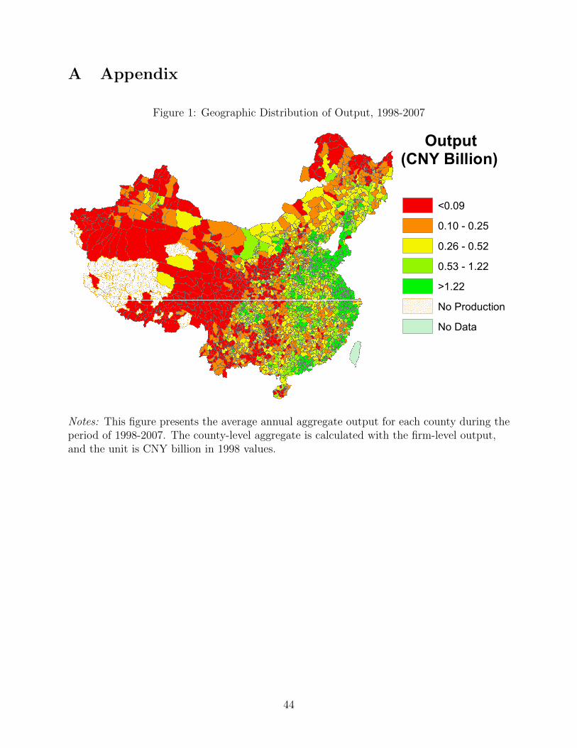
A Appendix

Figure 1: Geographic Distribution of Output, 1998-2007

<0.090.10 - 0.250.26 - 0.520.53 - 1.22>1.22No ProductionNo Data

Output(CNY Billion)

Notes: This figure presents the average annual aggregate output for each county during theperiod of 1998-2007. The county-level aggregate is calculated with the firm-level output,and the unit is CNY billion in 1998 values.

44

Figure 2: Distribution of Daily Temperatures, 1998-2007 and 2020-2049

020

4060

80

Ave

rage

Num

ber

of D

ays

per

Yea

r

<10F<-12C

10-20F-12--7C

20-30F-7--1C

30-40F<-1-4C

40-50F<4-10C

<50-60F10-16C

60-70F16-21C

70-80F21-27C

80-90F27-32C

>90F>32C

1998-2007 2020-2049

Notes: This figure illustrates the distribution of daily temperatures for the periods1998-2007 and 2020-2049. The “1998-2007” and “2020-2049” bars represent the averagenumber of days per year in each temperature category over these time periods. The climateprediction is obtained from the HadCM3 A1FI scenario.

45

Figure 3: Geographic Distribution of Changes in Days with Temperatures above 90◦F

<0.50.5-11-1.51.5-2>2No ProductionNo Data

Above 90F(Day)

Notes: This figure depicts the changes in days with temperatures above 90◦F under amedium-run climate change. The unit is the difference in days with temperatures above90◦F between the periods 2020-2049 and 1998-2007.

46

Fig

ure

4:E

ffec

tsof

Dai

lyT

emp

erat

ure

onO

utp

ut,

TF

P,

Lab

or,

and

Cap

ital

Inputs

Pan

elA

:T

emp

eratu

re-O

utp

ut

-.008-.006-.004-.0020.002

Log Output

<10

F<

-12C

10-2

0F-1

2--7

C20

-30F

-7--

1C30

-40F

<-1

-4C

40-5

0F<

4-10

C<

50-6

0F10

-16C

60-7

0F16

-21C

70-8

0F21

-27C

80-9

0F27

-32C

>90

F>

32C

Dai

ly T

empe

ratu

re

Est

imat

e95

% C

.I.

Pan

elB

:T

emp

eratu

re-T

FP

-.008-.006-.004-.0020.002

Log TFP

<10

F<

-12C

10-2

0F-1

2--7

C20

-30F

-7--

1C30

-40F

<-1

-4C

40-5

0F<

4-10

C<

50-6

0F10

-16C

60-7

0F16

-21C

70-8

0F21

-27C

80-9

0F27

-32C

>90

F>

32C

Dai

ly T

empe

ratu

re

Est

imat

e95

% C

.I.

Pan

elC

:T

emp

eratu

re-L

ab

or

-.008-.006-.004-.0020.002

Log Labor

<10

F<

-12C

10-2

0F-1

2--7

C20

-30F

-7--

1C30

-40F

<-1

-4C

40-5

0F<

4-10

C<

50-6

0F10

-16C

60-7

0F16

-21C

70-8

0F21

-27C

80-9

0F27

-32C

>90

F>

32C

Dai

ly T

empe

ratu

re

Est

imat

e95

% C

.I.

Pan

elD

:T

emp

eratu

re-C

ap

ital

-.008-.006-.004-.0020.002

Log Capital

<10

F<

-12C

10-2

0F-1

2--7

C20

-30F

-7--

1C30

-40F

<-1

-4C

40-5

0F<

4-10

C<

50-6

0F10

-16C

60-7

0F16

-21C

70-8

0F21

-27C

80-9

0F27

-32C

>90

F>

32C

Dai

ly T

empe

ratu

re

Est

imat

e95

% C

.I.

Notes:

Pan

elA

:E

stim

ated

Tem

per

ature

-Outp

ut

Rel

atio

nsh

ip.

Pan

elB

:E

stim

ated

Tem

per

ature

-TF

PR

elat

ionsh

ip.

Pan

elC

:E

stim

ated

Tem

per

ature

-Lab

orR

elat

ionsh

ip.

Pan

elD

:E

stim

ated

Tem

per

ature

-Cap

ital

Rel

atio

nsh

ip.

Reg

ress

ion

model

sar

ees

tim

ated

for

each

com

pon

ent

separ

atel

yusi

ng

Equat

ion

(7).

47

Fig

ure

5:E

ffec

tsof

Curr

ent

and

Lag

ged

Tem

per

ature

onO

utp

ut

and

TF

P

Pan

elA

:C

urr

ent

Tem

per

atu

re-O

utp

ut

-.008-.006-.004-.0020.002

Log Output

<10

F<

-12C

10-2

0F-1

2--7

C20

-30F

-7--

1C30

-40F

<-1

-4C

40-5

0F<

4-10

C<

50-6

0F10

-16C

60-7

0F16

-21C

70-8

0F21

-27C

80-9

0F27

-32C

>90

F>

32C

Cur

rent

Dai

ly T

empe

ratu

re

Est

imat

e95

% C

.I.

Pan

elB

:L

agged

Tem

per

atu

re-O

utp

ut

-.008-.006-.004-.0020.002

Log Output

<10

F<

-12C

10-2

0F-1

2--7

C20

-30F

-7--

1C30

-40F

<-1

-4C

40-5

0F<

4-10

C<

50-6

0F10

-16C

60-7

0F16

-21C

70-8

0F21

-27C

80-9

0F27

-32C

>90

F>

32C

Lagg

ed D

aily

Tem

pera

ture

Est

imat

e95

% C

.I.

Pan

elC

:C

urr

ent

Tem

per

atu

re-T

FP

-.008-.006-.004-.0020.002

Log TFP

<10

F<

-12C

10-2

0F-1

2--7

C20

-30F

-7--

1C30

-40F

<-1

-4C

40-5

0F<

4-10

C<

50-6

0F10

-16C

60-7

0F16

-21C

70-8

0F21

-27C

80-9

0F27

-32C

>90

F>

32C

Cur

rent

Dai

ly T

empe

ratu

re

Est

imat

e95

% C

.I.

Pan

elD

:L

agged

Tem

per

atu

re-T

FP

-.008-.006-.004-.0020.002

Log TFP

<10

F<

-12C

10-2

0F-1

2--7

C20

-30F

-7--

1C30

-40F

<-1

-4C

40-5

0F<

4-10

C<

50-6

0F10

-16C

60-7

0F16

-21C

70-8

0F21

-27C

80-9

0F27

-32C

>90

F>

32C

Lagg

ed D

aily

Tem

pera

ture

Est

imat

e95

% C

.I.

Notes:

Pan

elA

:E

stim

ated

Curr

ent

Tem

per

ature

-Outp

ut

Rel

atio

nsh

ip.

Pan

elB

:E

stim

ated

Lag

ged

Tem

per

ature

-Outp

ut

Rel

atio

nsh

ip.

Pan

elC

:E

stim

ated

Curr

ent

Tem

per

ature

-TF

PR

elat

ionsh

ip.

Pan

elD

:E

stim

ated

Lag

ged

Tem

per

ature

-TF

PR

elat

ionsh

ip.

Pan

els

Aan

dB

are

esti

mat

edsi

mult

aneo

usl

yin

one

regr

essi

on,

and

soar

epan

els

Can

dD

.

48

Fig

ure

6:E

ffec

tsof

Curr

ent

and

Lag

ged

Tem

per

ature

son

TF

PG

row

thR

ate

and

Inve

stm

ent

Pan

elA

:C

urr

ent

Tem

per

atu

re-T

FP

Gro

wth

Rate

-.004-.0020.002.004

TFP Growth Rate

<10

F<

-12C

10-2

0F-1

2--7

C20

-30F

-7--

1C30

-40F

<-1

-4C

40-5

0F<

4-10

C<

50-6

0F10

-16C

60-7

0F16

-21C

70-8

0F21

-27C

80-9

0F27

-32C

>90

F>

32C

Cur

rent

Dai

ly T

empe

ratu

re

Est

imat

e95

% C

.I.

Pan

elB

:L

agged

Tem

per

atu

re-T

FP

Gro

wth

Rate

-.004-.0020.002.004

TFP Growth Rate

<10

F<

-12C

10-2

0F-1

2--7

C20

-30F

-7--

1C30

-40F

<-1

-4C

40-5

0F<

4-10

C<

50-6

0F10

-16C

60-7

0F16

-21C

70-8

0F21

-27C

80-9

0F27

-32C

>90

F>

32C

Lagg

ed D

aily

Tem

pera

ture

Est

imat

e95

% C

.I.

Pan

elC

:C

urr

ent

Tem

per

atu

re-I

nve

stm

ent

-.02-.010.01.02.03

Log Investment

<10

F<

-12C

10-2

0F-1

2--7

C20

-30F

-7--

1C30

-40F

<-1

-4C

40-5

0F<

4-10

C<

50-6

0F10

-16C

60-7

0F16

-21C

70-8

0F21

-27C

80-9

0F27

-32C

>90

F>

32C

Cur

rent

Dai

ly T

empe

ratu

re

Est

imat

e95

% C

.I.

Pan

elD

:L

agged

Tem

per

atu

re-I

nve

stm

ent

-.02-.010.01.02.03

Log Investment

<10

F<

-12C

10-2

0F-1

2--7

C20

-30F

-7--

1C30

-40F

<-1

-4C

40-5

0F<

4-10

C<

50-6

0F10

-16C

60-7

0F16

-21C

70-8

0F21

-27C

80-9

0F27

-32C

>90

F>

32C

Lagg

ed D

aily

Tem

pera

ture

Est

imat

e95

% C

.I.

Notes:

Pan

elA

:E

stim

ated

Curr

ent

Tem

per

ature

-TF

PG

row

thR

ate

Rel

atio

nsh

ip.

Pan

elB

:E

stim

ated

Lag

ged

Tem

per

ature

-TF

PG

row

thR

ate

Rel

atio

nsh

ip.

Pan

elC

:E

stim

ated

Curr

ent

Tem

per

ature

-Inve

stm

ent

Rel

atio

nsh

ip.

Pan

elD

:E

stim

ated

Lag

ged

Tem

per

ature

-Inve

stm

ent

Rel

atio

nsh

ip.

Pan

els

Aan

dB

are

esti

mat

edsi

mult

aneo

usl

yin

one

regr

essi

on,

asar

epan

els

Can

dD

.

49

Fig

ure

7:E

ffec

tsof

Tem

per

ature

sA

bov

e90◦ F

onO

utp

ut

and

TF

Pfo

rE

ach

Sec

tor

Pan

elA

-2-1

01

2

Abo

ve 9

0F o

n O

utpu

t (%

)

Pro

cess

ing

of fo

ods

(5.7

8%)

Man

ufac

ture

of f

oods

(2.

21%

)

Bev

erag

es (

1.55

%)

Tex

tiles

(8.

41%

)

App

arel

(4.

35%

)

Leat

her

(2.2

2%)

Tim

ber

(2.0

9%)

Fur

nitu

re (

1.11

%)

Pap

er (

2.88

%)

Prin

ting

(1.8

8%)

Art

icle

s fo

r cu

lture

s an

d sp

orts

(1.

20%

)

Med

icin

es (

1.98

%)

Man

ufac

ture

of a

rtw

ork

(1.7

6%)

Non

-met

allic

min

eral

s (8

.17%

)

Gen

eral

mac

hine

ry (

7.33

%)

Raw

che

mic

als

(6.9

5%)

Ele

ctric

al m

achi

nery

(5.

56%

)

Met

al (

5.05

%)

Pla

stic

s (4

.40%

)

Tra

nspo

rt e

quip

men

t (4.

31%

)

Spe

cial

mac

hine

ry (

3.76

%)

Com

mun

icat

ion

equi

pmen

t (2.

83%

)

Sm

eltin

g of

ferr

ous

met

als

(2.1

9%)

Ele

ctric

ity a

nd h

eat (

1.81

%)

Sm

eltin

g of

non

-fer

rous

met

als

(1.6

6%)

Coa

l min

ing

(1.5

8%)

Mea

surin

g in

stru

men

ts (

1.31

%)

Rub

ber

(1.1

4%)

Non

met

al m

inin

g (0

.92%

)

Pet

role

um (

0.78

%)

Wat

er (

0.74

%)

Non

ferr

ous

met

al m

inin

g (0

.66%

)

Fer

rous

met

al m

inin

g (0

.61%

)

Pan

elB

-2-1

01

2

Abo

ve 9

0F o

n T

FP

(%

)

Pro

cess

ing

of fo

ods

(5.7

8%)

Man

ufac

ture

of f

oods

(2.

21%

)

Bev

erag

es (

1.55

%)

Tex

tiles

(8.

41%

)

App

arel

(4.

35%

)

Leat

her

(2.2

2%)

Tim

ber

(2.0

9%)

Fur

nitu

re (

1.11

%)

Pap

er (

2.88

%)

Prin

ting

(1.8

8%)

Art

icle

s fo

r cu

lture

s an

d sp

orts

(1.

20%

)

Med

icin

es (

1.98

%)

Man

ufac

ture

of a

rtw

ork

(1.7

6%)

Non

-met

allic

min

eral

s (8

.17%

)

Gen

eral

mac

hine

ry (

7.33

%)

Raw

che

mic

als

(6.9

5%)

Ele

ctric

al m

achi

nery

(5.

56%

)

Met

al (

5.05

%)

Pla

stic

s (4

.40%

)

Tra

nspo

rt e

quip

men

t (4.

31%

)

Spe

cial

mac

hine

ry (

3.76

%)

Com

mun

icat

ion

equi

pmen

t (2.

83%

)

Sm

eltin

g of

ferr

ous

met

als

(2.1

9%)

Ele

ctric

ity a

nd h

eat (

1.81

%)

Sm

eltin

g of

non

-fer

rous

met

als

(1.6

6%)

Coa

l min

ing

(1.5

8%)

Mea

surin

g in

stru

men

ts (

1.31

%)

Rub

ber

(1.1

4%)

Non

met

al m

inin

g (0

.92%

)

Pet

role

um (

0.78

%)

Wat

er (

0.74

%)

Non

ferr

ous

met

al m

inin

g (0

.66%

)

Fer

rous

met

al m

inin

g (0

.61%

)

Notes

:P

anel

A:

Eff

ect

ofT

emp

erat

ure

sA

bov

e90◦ F

onO

utp

ut.

Pan

elB

:E

ffec

tof

Tem

per

ature

sA

bov

e90◦ F

onT

FP

.T

he

shar

esof

the

sect

ors

inth

efu

llsa

mple

are

enum

erat

edin

the

par

enth

esis

.Sec

tors

are

sort

edac

cord

ing

toth

eir

shar

es.

All

tem

per

ature

bin

sar

ees

tim

ated

usi

ng

Equat

ion

(7),

alth

ough

the

effec

tsof

the

hig

hes

tte

mp

erat

ure

bin

alon

ear

ere

por

ted.

Lig

ht

indust

ries

are

lab

eled

inre

d,

wher

eas

hea

vy

indust

ries

are

inblu

e.

50

Fig

ure

8:C

lim

ate

Pre

dic

tion

son

Outp

ut

and

TF

Pfo

rE

ach

Sec

tor

Pan

elA

-20

-10

010

20

Clim

ate

Pre

dict

ion

on O

utpu

t (%

)

Pro

cess

ing

of fo

ods

(5.7

8%)

Man

ufac

ture

of f

oods

(2.

21%

)

Bev

erag

es (

1.55

%)

Tex

tiles

(8.

41%

)

App

arel

(4.

35%

)

Leat

her

(2.2

2%)

Tim

ber

(2.0

9%)

Fur

nitu

re (

1.11

%)

Pap

er (

2.88

%)

Prin

ting

(1.8

8%)

Art

icle

s fo

r cu

lture

s an

d sp

orts

(1.

20%

)

Med

icin

es (

1.98

%)

Man

ufac

ture

of a

rtw

ork

(1.7

6%)

Non

-met

allic

min

eral

s (8

.17%

)

Gen

eral

mac

hine

ry (

7.33

%)

Raw

che

mic

als

(6.9

5%)

Ele

ctric

al m

achi

nery

(5.

56%

)

Met

al (

5.05

%)

Pla

stic

s (4

.40%

)

Tra

nspo

rt e

quip

men

t (4.

31%

)

Spe

cial

mac

hine

ry (

3.76

%)

Com

mun

icat

ion

equi

pmen

t (2.

83%

)

Sm

eltin

g of

ferr

ous

met

als

(2.1

9%)

Ele

ctric

ity a

nd h

eat (

1.81

%)

Sm

eltin

g of

non

-fer

rous

met

als

(1.6

6%)

Coa

l min

ing

(1.5

8%)

Mea

surin

g in

stru

men

ts (

1.31

%)

Rub

ber

(1.1

4%)

Non

met

al m

inin

g (0

.92%

)

Pet

role

um (

0.78

%)

Wat

er (

0.74

%)

Non

ferr

ous

met

al m

inin

g (0

.66%

)

Fer

rous

met

al m

inin

g (0

.61%

)

Pan

elB

-20

-10

010

20

Clim

ate

Pre

dict

ion

on T

FP

(%

)

Pro

cess

ing

of fo

ods

(5.7

8%)

Man

ufac

ture

of f

oods

(2.

21%

)

Bev

erag

es (

1.55

%)

Tex

tiles

(8.

41%

)

App

arel

(4.

35%

)

Leat

her

(2.2

2%)

Tim

ber

(2.0

9%)

Fur

nitu

re (

1.11

%)

Pap

er (

2.88

%)

Prin

ting

(1.8

8%)

Art

icle

s fo

r cu

lture

s an

d sp

orts

(1.

20%

)

Med

icin

es (

1.98

%)

Man

ufac

ture

of a

rtw

ork

(1.7

6%)

Non

-met

allic

min

eral

s (8

.17%

)

Gen

eral

mac

hine

ry (

7.33

%)

Raw

che

mic

als

(6.9

5%)

Ele

ctric

al m

achi

nery

(5.

56%

)

Met

al (

5.05

%)

Pla

stic

s (4

.40%

)

Tra

nspo

rt e

quip

men

t (4.

31%

)

Spe

cial

mac

hine

ry (

3.76

%)

Com

mun

icat

ion

equi

pmen

t (2.

83%

)

Sm

eltin

g of

ferr

ous

met

als

(2.1

9%)

Ele

ctric

ity a

nd h

eat (

1.81

%)

Sm

eltin

g of

non

-fer

rous

met

als

(1.6

6%)

Coa

l min

ing

(1.5

8%)

Mea

surin

g in

stru

men

ts (

1.31

%)

Rub

ber

(1.1

4%)

Non

met

al m

inin

g (0

.92%

)

Pet

role

um (

0.78

%)

Wat

er (

0.74

%)

Non

ferr

ous

met

al m

inin

g (0

.66%

)

Fer

rous

met

al m

inin

g (0

.61%

)

Pan

elC -20

-10

010

20

Clim

ate

Pre

dict

ion

on O

utpu

t (C

NY

Bill

ion)

Pro

cess

ing

of fo

ods

(5.7

8%)

Man

ufac

ture

of f

oods

(2.2

1%)

Bev

erag

es (1

.55%

)

Text

iles

(8.4

1%)

App

arel

(4.3

5%)

Leat

her (

2.22

%)

Tim

ber (

2.09

%)

Furn

iture

(1.1

1%)

Pap

er (2

.88%

)

Prin

ting

(1.8

8%)

Arti

cles

for c

ultu

res

and

spor

ts (1

.20%

)

Med

icin

es (1

.98%

)

Man

ufac

ture

of a

rtwor

k (1

.76%

)

Non

-met

allic

min

eral

s (8

.17%

)

Gen

eral

mac

hine

ry (7

.33%

)

Raw

che

mic

als

(6.9

5%)

Ele

ctric

al m

achi

nery

(5.5

6%)

Tran

spor

t equ

ipm

ent (

4.31

%)

Met

al (5

.05%

)

Pla

stic

s (4

.40%

)

Spe

cial

mac

hine

ry (3

.76%

)

Com

mun

icat

ion

equi

pmen

t (2.

83%

)

Rub

ber (

1.14

%)

Ele

ctric

ity a

nd h

eat (

1.81

%)

Mea

surin

g in

stru

men

ts (1

.31%

)

Sm

eltin

g of

ferr

ous

met

als

(2.1

9%)

Non

met

al m

inin

g (0

.92%

)

Pet

role

um (0

.78%

)

Wat

er (0

.74%

)

Non

ferr

ous

met

al m

inin

g (0

.66%

)

Ferr

ous

met

al m

inin

g (0

.61%

)

Sm

eltin

g of

non

-ferr

ous

met

als

(1.6

6%)

Coa

l min

ing

(1.5

8%)

Notes:

Pan

elA

:C

lim

ate

Pre

dic

tion

onO

utp

ut

inP

erce

nta

geP

oints

.P

anel

B:

Clim

ate

Pre

dic

tion

onT

FP

.P

anel

C:

Clim

ate

Pre

dic

tion

onO

utp

ut

inC

NY

Billion

.T

he

shar

esof

the

obse

rvat

ions

inth

efu

llsa

mple

ofal

lse

ctor

sar

elist

edin

the

par

enth

esis

.In

pan

els

Aan

dB

,se

ctor

sar

eso

rted

acco

rdin

gto

thei

rsh

ares

.In

pan

elC

,se

ctor

sar

eso

rted

bas

edon

thei

rcl

imat

eim

pac

ts.

Lig

ht

indust

ries

are

lab

eled

inre

d,

wher

eas

hea

vy

indust

ries

are

inblu

e.

51

Fig

ure

9:C

lim

ate

Pre

dic

tion

son

Outp

ut

and

TF

Pfo

rE

ach

Cou

nty

Pan

elA

<-6 -6- -4

-4- -2

-2-0

>0 No Pr

oduc

tion

No D

ata

Outpu

t (%)

Pan

elB

<-0.06

-0.06

- -0.04

-0.04

- -0.02

-0.02

-0>0 No

Prod

uctio

nNo

Data

Outpu

t (C

NY

Billio

n)

Pan

elC

<-6 -6- -4

-4- -2

-2-0

>0 No Pr

oduc

tion

No D

ata

TFP (

%)P

an

elC

<0.5

0.5-1

1-1.5

1.5-2

>2 No Pr

oduc

tion

No D

ata

Abov

e 90F

(Day

)

Notes:

Pan

elA

:C

lim

ate

Pre

dic

tion

onO

utp

ut

inP

erce

nta

geP

oints

.P

anel

B:

Clim

ate

Pre

dic

tion

onO

utp

ut

inC

NY

Billion

.P

anel

C:

Clim

ate

Pre

dic

tion

onT

FP

.P

anel

D:

Chan

ges

inD

ays

wit

hT

emp

erat

ure

sA

bov

e90◦ F

bet

wee

nth

eP

erio

ds

2020

-204

9an

d19

98-2

007.

52

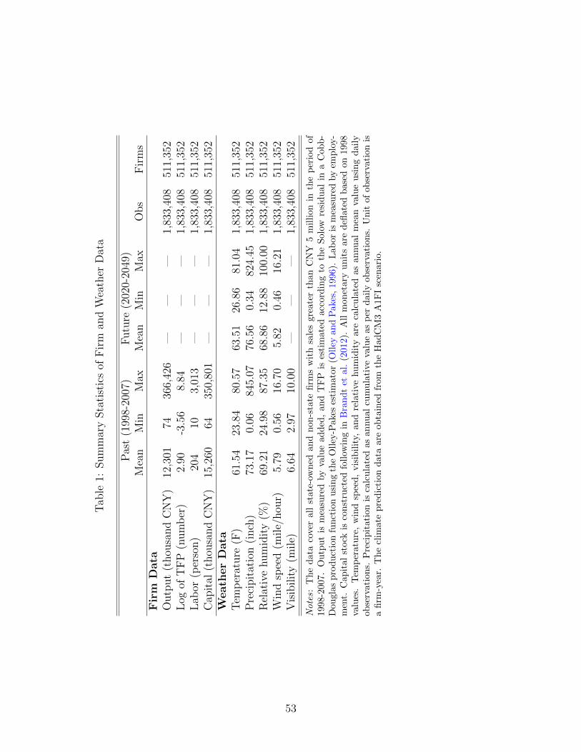
Tab

le1:

Sum

mar

ySta

tist

ics

ofF

irm

and

Wea

ther

Dat

a

Pas

t(1

998-

2007

)F

utu

re(2

020-

2049

)M

ean

Min

Max

Mea

nM

inM

axO

bs

Fir

ms

Fir

mD

ata

Outp

ut

(thou

sand

CN

Y)

12,3

0174

366,

426

——

—1,

833,

408

511,

352

Log

ofT

FP

(num

ber

)2.

90-3

.56

8.84

——

—1,

833,

408

511,

352

Lab

or(p

erso

n)

204

103,

013

——

—1,

833,

408

511,

352

Cap

ital

(thou

sand

CN

Y)

15,2

6064

350,

801

——

—1,

833,

408

511,

352

Weath

er

Data

Tem

per

ature

(F)

61.5

423

.84

80.5

763

.51

26.8

681

.04

1,83

3,40

851

1,35

2P

reci

pit

atio

n(i

nch

)73

.17

0.06

845.

0776

.56

0.34

824.

451,

833,

408

511,

352

Rel

ativ

ehum

idit

y(%

)69

.21

24.9

887

.35

68.8

612

.88

100.

001,

833,

408

511,

352

Win

dsp

eed

(mile/

hou

r)5.

790.

5616

.70

5.82

0.46

16.2

11,

833,

408

511,

352

Vis

ibilit

y(m

ile)

6.64

2.97

10.0

0—

——

1,83

3,40

851

1,35

2

Notes:

Th

ed

ata

cove

ral

lst

ate-

own

edan

dn

on

-sta

tefi

rms

wit

hsa

les

gre

ate

rth

an

CN

Y5

mil

lion

inth

ep

erio

dof

1998

-200

7.O

utp

ut

ism

easu

red

by

valu

ead

ded

,an

dT

FP

ises

tim

ate

dacc

ord

ing

toth

eS

olo

wre

sid

ual

ina

Cob

b-

Dou

glas

pro

du

ctio

nfu

nct

ion

usi

ng

the

Oll

ey-P

ake

ses

tim

ato

r(O

lley

an

dP

ake

s,1996).

Lab

or

ism

easu

red

by

emp

loy-

men

t.C

apit

alst

ock

isco

nst

ruct

edfo

llow

ing

inB

ran

dt

etal.

(2012).

All

mon

etary

un

its

are

defl

ate

db

ase

don

1998

valu

es.

Tem

per

atu

re,

win

dsp

eed

,vis

ibilit

y,an

dre

lati

vehu

mid

ity

are

calc

ula

ted

as

an

nu

al

mea

nva

lue

usi

ng

dail

yob

serv

atio

ns.

Pre

cipit

atio

nis

calc

ula

ted

as

an

nu

al

cum

ula

tive

valu

eas

per

dail

yob

serv

ati

on

s.U

nit

of

ob

serv

ati

on

isa

firm

-yea

r.T

he

clim

ate

pre

dic

tion

data

are

ob

tain

edfr

om

the

HadC

M3

A1F

Isc

enari

o.

53

Tab

le2:

Eff

ects

ofT

emp

erat

ure

onO

utp

ut

and

TF

P

TF

Pby

OP

TF

Pby

Ind

ex

Mea

nT

emp

Max

Tem

pH

eat

Ind

exM

ean

Tem

(1a)

(1b

)(1

c)(1

d)

(2a)

(2b)

(3)

Ou

tpu

t

80-9

0◦F

-0.0

009*

*-0

.003

4***

-0.0

007*

*-0

.003

4***

0.00

05-0

.0024***

-0.0

034***

(0.0

004)

(0.0

004)

(0.0

004)

(0.0

005)

(0.0

004)

(0.0

005)

(0.0

005)

>90◦ F

-0.0

028*

**-0

.004

7***

-0.0

022*

**-0

.004

5***

-0.0

010*

*-0

.0046***

-0.0

045***

(0.0

008)

(0.0

009)

(0.0

008)

(0.0

009)

(0.0

004)

(0.0

005)

(0.0

009)

F-s

tati

stic

(All

Bin

s)11

.78*

**11

.81*

**10

.83*

**11

.61*

**14

.08*

**13.9

5***

11.6

1***

TF

P

80-9

0◦F

-0.0

011*

**-0

.002

4***

-0.0

009*

**-0

.002

4***

0.00

07*

-0.0

018***

-0.0

015***

(0.0

003)

(0.0

004)

(0.0

003)

(0.0

004)

(0.0

004)

(0.0

004)

(0.0

003)

>90◦ F

-0.0

041*

**-0

.005

7***

-0.0

036*

**-0

.005

6***

-0.0

009*

*-0

.0033***

-0.0

029***

(0.0

007)

(0.0

008)

(0.0

007)

(0.0

008)

(0.0

004)

(0.0

004)

(0.0

007)

F-s

tati

stic

(All

Bin

s)12

.28*

**11

.64*

**11

.41*

**11

.40*

**12

.45*

**12.4

6***

8.2

8***

Ob

serv

atio

ns

1,83

3,40

81,

833,

408

1,83

3,40

81,

833,

408

1,83

3,40

81,8

33,4

08

1,8

33,4

08

Fir

mF

EY

ES

YE

SY

ES

YE

SY

ES

YE

SY

ES

Yea

rF

EY

ES

NO

NO

NO

NO

NO

NO

Yea

r-by-r

egio

nF

EN

OY

ES

NO

YE

SY

ES

YE

SY

ES

Yea

r-by-t

wo-

dig

it-s

ecto

rF

EN

ON

OY

ES

YE

SY

ES

YE

SY

ES

Notes:

Th

ed

epen

den

tva

riab

les

are

loga

rith

ms

of

ou

tpu

tan

dT

FP

.R

egre

ssio

nm

od

els

are

esti

mate

du

sin

gE

qu

ati

on

(7).

Th

rou

gh

colu

mn

s(1

a)-(

2b),

TF

Pis

mea

sure

dby

Oll

ey-P

akes

esti

mato

r.In

colu

mn

(3),

TF

Pis

mea

sure

dw

ith

the

ind

exnu

mb

erap

pro

ach

.B

ins

are

con

-st

ruct

edac

cord

ing

tod

aily

mea

nte

mp

erat

ure

as

per

colu

mn

s(1

a)-

(1d

).In

colu

mn

s(2

a)

an

d(2

b),

bin

sar

eco

nst

ruct

edu

sin

gd

ail

ym

ax-

imu

mte

mp

erat

ure

and

dai

lyh

eat

ind

ex.

Colu

mn

(1d

)is

the

base

lin

esp

ecifi

cati

on

thro

ugh

ou

tth

est

ud

y.D

ue

tosp

ace

lim

itati

on

s,w

ere

por

ton

lyth

eeff

ects

ofth

etw

oh

igh

est

tem

per

atu

reb

ins.

Sta

ndard

erro

rsare

clu

ster

edat

both

firm

an

dco

unty

-yea

rle

vel

s.∗p<

0.1

0,

∗∗p<

0.05

,∗∗∗p<

0.01

.S

eeth

ete

xt

for

more

det

ail

s.

54

Table 3: Effects of Temperature on TFP between Labor- and Capital-Intensive Firms

Intensity = Wage Bill/Output Intensity = Labor/Sales

(1a) (1b) (1c) (2a) (2b) (2c)

80-90◦F -0.0035*** -0.0030*** -0.0029*** -0.0024*** -0.0024*** -0.0022***(0.0003) (0.0003) (0.0003) (0.0004) (0.0004) (0.0004)

>90◦F -0.0042*** -0.0081*** -0.0076*** -0.0055*** -0.0083*** -0.0062***(0.0008) (0.0007) (0.0007) (0.0008) (0.0008) (0.0008)

80-90◦F × Labor Intensity 0.0041*** — — -0.0001 — —(0.0003) — — (0.0002) — —

>90◦F × Labor Intensity -0.0008 — — -0.0094 — —(0.0016) — — (0.0060) — —

80-90◦F × Above Median — 0.0009*** — — 0.0008*** —— (0.0001) — — (0.0001) —

>90◦× Above Median — 0.0064*** — — 0.0072*** —— (0.0006) — — (0.0006) —

80-90◦F × Above Mean — — 0.0010*** — — 0.0004***— — (0.0001) — — (0.0001)

>90◦× Above Mean — — 0.0061*** — — 0.0042***— — (0.0006) — — (0.0008)

Observations 1,833,408 1,833,408 1,833,408 1,833,408 1,833,408 1,833,408

Notes: The dependent variable is the log of TFP. Regression models are estimated using Equation (7) and includefirm fixed effects, year-by-region fixed effects, and year-by-two-digit-sector fixed effects. In columns (1a)-(1c), laborintensity is measured by wage bill/output. In columns (2a)-(2c), labor intensity is determined through labor/sales. Incolumns (1a) and (2a), we interact the two highest temperature bins with raw labor intensity. In columns (1b) and(2b), labor intensity is classified as either above median (=1) or below median (=0); subsequently, we interact the twohighest temperature bins with a dummy variable for above median. The dummy variable for below median is omittedfor multicollinearity. In columns (1c) and (2c), labor intensity is classified as either above mean (=1) or below mean(=0); then, we interact the two highest temperatures bins with a dummy variable for above mean. The dummy vari-able for below mean is omitted for multicollinearity. Due to space limitations, we report only the effects of the twohighest temperature bins. Standard errors are clustered at both firm and county-year levels. ∗ p <0.10, ∗∗ p <0.05,∗∗∗ p <0.01. See the text for more details.

55

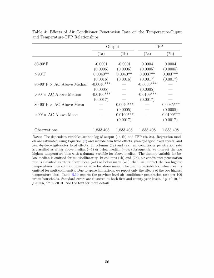
Table 4: Effects of Air Conditioner Penetration Rate on the Temperature-Ouputand Temperature-TFP Relationships

Output TFP

(1a) (1b) (2a) (2b)

80-90◦F -0.0001 -0.0001 0.0004 0.0004(0.0006) (0.0006) (0.0005) (0.0005)

>90◦F 0.0040** 0.0040** 0.0037** 0.0037**(0.0016) (0.0016) (0.0017) (0.0017)

80-90◦F × AC Above Median -0.0040*** — -0.0035*** —(0.0005) — (0.0005) —

>90◦× AC Above Median -0.0100*** — -0.0109*** —(0.0017) — (0.0017) —

80-90◦F × AC Above Mean — -0.0040*** — -0.0035***— (0.0005) — (0.0005)

>90◦× AC Above Mean — -0.0100*** — -0.0109***— (0.0017) — (0.0017)

Observations 1,833,408 1,833,408 1,833,408 1,833,408

Notes: The dependent variables are the log of output (1a-1b) and TFP (2a-2b). Regression mod-els are estimated using Equation (7) and include firm fixed effects, year-by-region fixed effects, andyear-by-two-digit-sector fixed effects. In columns (1a) and (2a), air conditioner penetration rateis classified as either above median (=1) or below median (=0); subsequently, we interact the twohighest temperature bins with a dummy variable for above median. The dummy variable for be-low median is omitted for multicollinearity. In columns (1b) and (2b), air conditioner penetrationrate is classified as either above mean (=1) or below mean (=0); then, we interact the two highesttemperatures bins with a dummy variable for above mean. The dummy variable for below mean isomitted for multicollinearity. Due to space limitations, we report only the effects of the two highesttemperature bins. Table B.10 reports the province-level air conditioner penetration rate per 100urban households. Standard errors are clustered at both firm and county-year levels. ∗ p <0.10, ∗∗

p <0.05, ∗∗∗ p <0.01. See the text for more details.

56

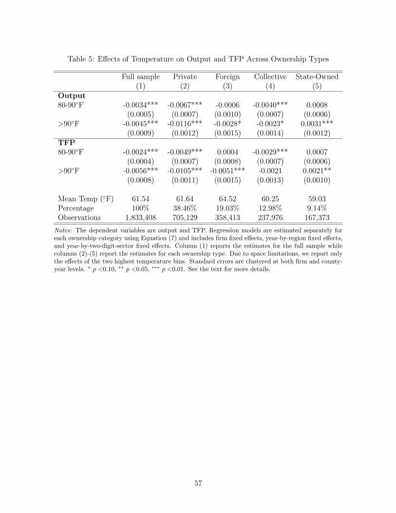
Table 5: Effects of Temperature on Output and TFP Across Ownership Types

Full sample Private Foreign Collective State-Owned(1) (2) (3) (4) (5)

Output80-90◦F -0.0034*** -0.0067*** -0.0006 -0.0040*** 0.0008

(0.0005) (0.0007) (0.0010) (0.0007) (0.0006)>90◦F -0.0045*** -0.0116*** -0.0028* -0.0023* 0.0031***

(0.0009) (0.0012) (0.0015) (0.0014) (0.0012)TFP80-90◦F -0.0024*** -0.0049*** 0.0004 -0.0029*** 0.0007

(0.0004) (0.0007) (0.0008) (0.0007) (0.0006)>90◦F -0.0056*** -0.0105*** -0.0051*** -0.0021 0.0021**

(0.0008) (0.0011) (0.0015) (0.0013) (0.0010)

Mean Temp (◦F) 61.54 61.64 64.52 60.25 59.03Percentage 100% 38.46% 19.03% 12.98% 9.14%Observations 1,833,408 705,129 358,413 237,976 167,373

Notes: The dependent variables are output and TFP. Regression models are estimated separately foreach ownership category using Equation (7) and includes firm fixed effects, year-by-region fixed effects,and year-by-two-digit-sector fixed effects. Column (1) reports the estimates for the full sample whilecolumns (2)-(5) report the estimates for each ownership type. Due to space limitations, we report onlythe effects of the two highest temperature bins. Standard errors are clustered at both firm and county-year levels. ∗ p <0.10, ∗∗ p <0.05, ∗∗∗ p <0.01. See the text for more details.

57

Tab

le6:

Eff

ects

ofT

emp

erat

ure

onT

FP

acro

ssR

egio

ns

Eco

nom

icR

egio

nO

vera

llN

orth

east

Eas

tC

entr

alW

est

(1a)

(1b)

(1c)

(1d)

(1e)

80-9

0◦F

-0.0

024*

**-0

.000

4-0

.004

5***

-0.0

035*

**0.

0003

(0.0

004)

(0.0

019)

(0.0

007)

(0.0

008)

(0.0

006)

>90◦ F

-0.0

056*

**0.

0187

-0.0

100*

**0.

0013

0.00

04(0

.000

8)(0

.016

4)(0

.001

4)(0

.001

3)(0

.001

3)M

ean

TF

P2.

902.

712.

982.

852.

63O

bse

rvat

ions

1,83

3,40

811

1,50

61,

226,

702

298,

702

196,

498

Geogra

phic

Regio

nO

vera

llN

orth

Nor

thea

stE

ast

Cen

tral

Sou

thSou

thw

est

Nor

thw

est

(2a)

(2b)

(2c)

(2d)

(2e)

(2f)

(2g)

(2h)

80-9

0◦F

-0.0

024*

**-0

.005

9***

-0.0

004

-0.0

041*

**-0

.005

2***

-0.0

022

0.00

04-0

.000

2(0

.000

4)(0

.001

3)(0

.001

9)(0

.000

7)(0

.001

3)(0

.001

3)(0

.000

8)(0

.001

3)>

90◦ F

-0.0

056*

**-0

.011

8***

0.01

87-0

.008

1***

-0.0

023

-0.0

213*

**0.

0016

0.00

25(0

.000

8)(0

.004

5)(0

.017

4)(0

.001

2)(0

.001

7)(0

.005

8)(0

.001

5)(0

.003

2)M

ean

Tem

p(◦

F)

61.5

453

.99

46.7

762

.27

61.4

573

.20

61.7

450

.93

Obse

rvat

ions

1,83

3,40

818

2,18

911

1,50

693

6,47

820

0,39

724

6,51

510

6,67

649

,647

Notes:

Th

ed

epen

den

tva

riab

leis

TF

P.

Reg

ress

ion

mod

els

are

esti

mate

dse

para

tely

for

each

regio

nu

sin

gE

qu

ati

on

(7).

Inth

efi

rst

pan

el,

firm

sare

clas

sifi

edac

cord

ing

toth

eir

resp

ecti

veec

onom

icre

gio

ns.

Inth

ese

con

dp

an

el,

firm

sare

class

ified

base

don

geo

gra

ph

icre

gio

ns.

Th

ere

gio

ncl

ass

ifica

tion

isd

etai

led

inT

able

B.8

inth

eon

lin

eap

pen

dix

.W

eals

ore

port

the

aver

age

an

nu

al

mea

nte

mp

eratu

refo

rea

chgeo

gra

ph

icre

gio

nan

dth

eav

erage

TF

Pfo

rea

chec

onom

icre

gion

.D

ue

tosp

ace

lim

itat

ion

s,w

ep

rese

nt

on

lyth

eeff

ects

of

the

two

hig

hes

tte

mp

eratu

rebin

s.S

tan

dard

erro

rsare

clu

ster

edat

bot

hfi

rman

dco

unty

-yea

rle

vels

.∗p<

0.10

,∗∗p<

0.0

5,∗∗∗p<

0.0

1.

See

the

text

for

more

det

ail

s.

58

Tab

le7:

Clim

ate

Pre

dic

tion

son

Outp

ut

and

TF

P

Full

Sam

ple

Pri

vate

For

eign

Col

lect

ive

Sta

te-O

wned

(1)

(2)

(3)

(4)

(5)

Outp

ut

(%)

Poi

nt

Est

imat

e-5

.71

-11.

26-2

.56

-3.4

8-0

.26

S.E

.0.

611.

021.

510.

890.

7395

%C

.I.

[-6.

91,

-4.5

1][-

13.2

5,-9

.27]

[-5.

52,

0.39

][-

5.23

,-1

.73]

[-1.

71,

1.18

]O

utp

ut

(CN

YB

illi

on)

Poi

nt

Est

imat

e-2

08.3

2-1

68.7

2-2

7.11

-10.

91-0

.68

S.E

.22

.27

15.2

215

.94

2.80

1.89

95%

C.I

.[-

251.

97,

-164

.68]

[-19

8.55

,-1

38.9

0][-

58.3

6,4.

14]

[-16

.40,

-5.4

1][-

4.39

,3.

03]

TF

PP

oint

Est

imat

e(%

)-4

.18

-8.3

2-0

.81

-1.8

3-0

.35

S.E

.(%

)0.

550.

961.

270.

860.

7595

%C

.I.

(%)

[-5.

27,

-3.1

0][-

10.2

0,-6

.44]

[-3.

31,

1.68

][-

3.51

,-0

.15]

[-1.

81,

1.12

]O

wner

ship

Per

centa

ge10

0%38

.46%

19.0

3%12

.98%

9.14

%

Notes:

Th

eto

pp

art

pre

sents

the

clim

ate

pre

dic

tion

on

ou

tpu

tin

per

centa

ge

poin

ts.

Th

em

idd

lep

art

pre

sents

the

clim

ate

pre

dic

tion

onou

tpu

tin

CN

Yb

illi

onin

2013

valu

es.

Th

eb

ott

om

part

pre

sents

the

clim

ate

pre

dic

tion

on

TF

P.

59

B Online Appendix

B.1 Data

B.1.1 Calculating Relative Humidity using Temperature and Dew Point Tem-

perature

The NOAA does not report data on relative humidity. Thus, we use the following meteoro-

logical formula provided by the NOAA to calculate relative humidity:39

RH ≈ 100(112− 0.1T + Td

112 + 0.9T)8, (9)

where RH denotes relative humidity in percent, T represents the air temperature in ◦C, and

Td represents the dew point temperature in ◦C.

B.1.2 Calculating Heat Index using Temperature and Relative Humidity

Heat index, or the apparent temperature, is an index that measures the sensation of tem-

perature when combined with humidity. The human body can cool itself down through

perspiration; however, this process is hard in a humid environment. For example, if the air

temperature is 90◦F and the relative humidity is 60%, then the air temperature feels as if it

is at 100◦F.40

To calculate heat index, we use the following formula provided by the National Weather

Service:41

HI = −42.379 + 2.04901523 ∗ T + 10.14333127 ∗RH − .22475541 ∗ T ∗RH

−.00683783 ∗ T ∗ T − .05481717 ∗RH ∗RH + .00122874 ∗ T ∗ T ∗RH

+.00085282 ∗ T ∗RH ∗RH − .00000199 ∗ T ∗ T ∗RH ∗RH,

(10)

39http://www.erh.noaa.gov/bgm/tables/rh.shtml40http://www.srh.noaa.gov/ama/?n=heatindex41http://www.wpc.ncep.noaa.gov/html/heatindex_equation.shtml

60

where HI represents heat index in ◦F, T denotes temperature in ◦F, and RH indicates

relative humidity in percent.

When the relative humidity is less than 13% and the temperature is between 80-112◦F,

the following formula is used to calculate the heat index:

HI = −42.379 + 2.04901523 ∗ T + 10.14333127 ∗RH − .22475541 ∗ T ∗RH

−.00683783 ∗ T ∗ T − .05481717 ∗RH ∗RH + .00122874 ∗ T ∗ T ∗RH

+.00085282 ∗ T ∗RH ∗RH − .00000199 ∗ T ∗ T ∗RH ∗RH

−((13−RH)/4) ∗ ((17− |T − 95|)/17)0.5.

(11)

On the other hand, if the relative humidity is larger than 85% and the temperature is

between 80-87◦F, we use the following formula:

HI = −42.379 + 2.04901523 ∗ T + 10.14333127 ∗RH − .22475541 ∗ T ∗RH

−.00683783 ∗ T ∗ T − .05481717 ∗RH ∗RH + .00122874 ∗ T ∗ T ∗RH

+.00085282 ∗ T ∗RH ∗RH − .00000199 ∗ T ∗ T ∗RH ∗RH

+((RH − 85)/10) ∗ (87− T )/5).

(12)

Lastly, if the calculated heat index from above formulas is smaller than 80◦F, the following

formula is used:

HI = 0.5 ∗ (T + 61.0 + ((T − 68.0) ∗ 1.2) + (RH ∗ 0.094)). (13)

B.2 Figures and Tables

61

Figure B.10: Distribution of Weather Stations in China. Notes : Each dot represents aweather station and each polygon represents a county.

62

Table B.8: Region Classification

Geographic Regions ProvincesNorth Beijing, Tianjin, Hebei, Shanxi, Nei MongolNortheast Liaoning, Jilin, HeilongjiangEast Shanghai, Jiangsu, Zhejiang, Anhui, Fujian, Jiangxi, ShandongCentral Henan, Hubei, HunanSouth Guangdong, Guangxi, HainanSouthwest Chongqing, Sichuan, Guizhou, Yunan, Xizang (Tibet)Northwest Shaanxi, Gansu, Qinghai, Ningxia Hui, Xinjiang UygurEconomic Regions ProvincesNortheast Liaoning, Jilin, HeilongjiangEast Beijing, Tianjin, Hebei, Shanghai, Jiangsu, Zhejiang,

Fujian, Shandong, Guangdong, HainanCentral Shanxi, Anhui, Jiangxi, Henan, Hubei, HunanWest Nei Mongol, Guangxi, Chongqing, Sichuan, Guizhou, Yunnan,

Xizang (Tibet), Shaanxi, Gansu, Qinghai, Ningxia Hui, Xinjiang Uygur

Notes: Geographic regions are classified based on traditional standards. Economic regions are classified accordingto the standards published on the NBS website http://www.stats.gov.cn/ztjc/zthd/sjtjr/dejtjkfr/tjkp/

201106/t20110613_71947.htm.

63

Table B.9: Regression Results for Climate Vari-ables Other than Temperature

Output TFP(1) (2)

Precipitation -0.0005*** -0.0004***(0.0001) (0.0001)

Precipitation Square 0.0000 0.0000(0.0000) (0.0000)

Humidity -0.0011 -0.0015(0.0010) (0.0010)

Humidity Square 0.0000 0.0000(0.0000) (0.0000)

Wind Speed -0.0116 -0.0202**(0.0104) (0.0094)

Wind Speed Square -0.0016** -0.0001(0.0008) (0.0007)

Visibility -0.0456* -0.0341(0.0277) (0.0241)

Visibility Square 0.0032 0.0025(0.0020) (0.0018)

Observations 1,833,408 1,833,408

Notes: This table supplements Table 2. The dependentvariables are logarithms of output and TFP. Regressionmodels are estimated using Equation (7). This tablereports additional estimates for climatic variables otherthan temperature. ∗ p <0.10, ∗∗ p <0.05, ∗∗∗ p <0.01.

64

Table B.10: Air Conditioner Penetration Rate per100 Urban Households

Provinces AC Penetration Rate IntensityGuangdong 126.68 HighShanghai 124.74 High

Chongqing 113.13 HighBeijing 101.31 High

Zhejiang 95.77 HighTianjin 82.70 HighFujian 82.00 HighJiangsu 77.80 HighHubei 66.27 HighHenan 60.60 HighAnhui 54.14 HighHunan 53.92 HighHeibei 51.60 High

Shaanxi 47.07 HighShandong 46.61 HighGuangxi 46.18 HighJiangxi 42.71 LowSichuan 42.67 LowHainan 28.78 LowShanxi 14.28 Low

Liaoning 8.69 LowGuizhou 6.07 Low

Xinjiang Uygur 4.66 LowNei Mongol 3.95 LowHeilongjiang 3.74 LowNingxia Hui 3.11 Low

Jilin 2.88 LowXizang (Tibet) 2.79 Low

Gansu 1.92 LowYunnan 0.50 LowQinghai 0.31 Low

China 53.21

Notes: This table presents the average air conditioner pene-tration rate per 100 urban households in each province overthe periods 1998-2007 in China. The provinces are sorted bythe air conditioner penetration rate. The last row reports theaverage air conditioner penetration rate for the whole China.Provinces are classified by either high intensity (above me-dian) or low intensity (below median) based on the median ofair conditioner penetration rate.

65

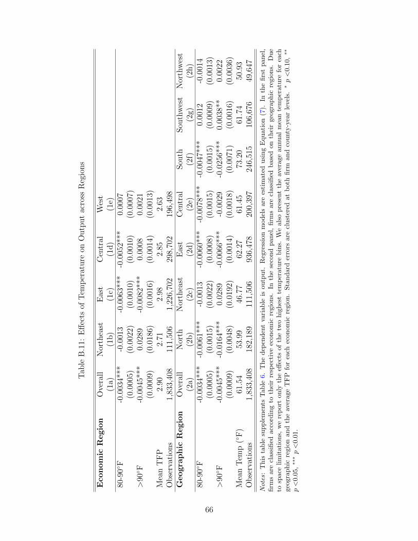
Tab

leB

.11:

Eff

ects

ofT

emp

erat

ure

onO

utp

ut

acro

ssR

egio

ns

Eco

nom

icR

egio

nO

vera

llN

orth

east

Eas

tC

entr

alW

est

(1a)

(1b)

(1c)

(1d)

(1e)

80-9

0◦F

-0.0

034*

**-0

.001

3-0

.006

3***

-0.0

052*

**0.

0007

(0.0

005)

(0.0

022)

(0.0

010)

(0.0

010)

(0.0

007)

>90◦ F

-0.0

045*

**0.

0289

-0.0

082*

**0.

0008

0.00

21(0

.000

9)(0

.018

6)(0

.001

6)(0

.001

4)(0

.001

3)M

ean

TF

P2.

902.

712.

982.

852.

63O

bse

rvat

ions

1,83

3,40

811

1,50

61,

226,

702

298,

702

196,

498

Geogra

phic

Regio

nO

vera

llN

orth

Nor

thea

stE

ast

Cen

tral

Sou

thSou

thw

est

Nor

thw

est

(2a)

(2b)

(2c)

(2d)

(2e)

(2f)

(2g)

(2h)

80-9

0◦F

-0.0

034*

**-0

.006

1***

-0.0

013

-0.0

060*

**-0

.007

8***

-0.0

047*

**0.

0012

-0.0

014

(0.0

005)

(0.0

015)

(0.0

022)

(0.0

008)

(0.0

015)

(0.0

015)

(0.0

009)

(0.0

013)

>90◦ F

-0.0

045*

**-0

.016

4***

0.02

89-0

.006

6***

-0.0

029

-0.0

256*

**0.

0038

**0.

0022

(0.0

009)

(0.0

048)

(0.0

192)

(0.0

014)

(0.0

018)

(0.0

071)

(0.0

016)

(0.0

036)

Mea

nT

emp

(◦F

)61

.54

53.9

946

.77

62.2

761

.45

73.2

061

.74

50.9

3O

bse

rvat

ions

1,83

3,40

818

2,18

911

1,50

693

6,47

820

0,39

724

6,51

510

6,67

649

,647

Notes:

Th

ista

ble

sup

ple

men

tsT

able

6.T

he

dep

end

ent

vari

ab

leis

ou

tput.

Reg

ress

ion

mod

els

are

esti

mate

du

sin

gE

qu

ati

on

(7).

Inth

efi

rst

pan

el,

firm

sar

ecl

assi

fied

acco

rdin

gto

thei

rre

spec

tive

econ

om

icre

gio

ns.

Inth

ese

con

dp

an

el,

firm

sare

class

ified

bas

edon

thei

rgeo

gra

ph

icre

gio

ns.

Du

eto

spac

eli

mit

atio

ns,

we

rep

ort

only

the

effec

tsof

the

two

hig

hes

tte

mp

eratu

reb

ins.

We

als

op

rese

nt

the

aver

age

an

nu

al

mea

nte

mp

eratu

refo

rea

chge

ogra

ph

icre

gion

and

the

aver

age

TF

Pfo

rea

chec

on

om

icre

gio

n.

Sta

nd

ard

erro

rsare

clu

ster

edat

both

firm

and

cou

nty

-yea

rle

vels

.∗p<

0.1

0,∗∗

p<

0.05

,∗∗∗p<

0.01

.

66