Temperature Changes in Different Layers of Cable Joints ...
71
Temperature Changes in Different Layers of Cable Joints and Insulation Electrical Power Engineering Chair of High Voltage Engineering Master thesis Head of Chair Prof J. Valtin Supervisors Prof P. Hyvönen, Sr researcher P. Taklaja Student S. Nopri Tallinn 2015
Transcript of Temperature Changes in Different Layers of Cable Joints ...

Temperature Changes in Different
Layers of Cable Joints and Insulation
Electrical Power Engineering
Chair of High Voltage Engineering
Master thesis
Head of Chair Prof J. Valtin
Supervisors Prof P. Hyvönen,
Sr researcher P. Taklaja
Student S. Nopri
Tallinn 2015

Declaration of Authorship
I hereby declare that this thesis is the result of my own independent work and it has been
presented to the department of Electrical Power Engineering of Tallinn University of
Technology in order to claim a master’s diploma in Electrical Power Engineering. This thesis has
not been presented before to claim a degree in engineering sciences or engineering.
Student (date and signature) _________________________________

Summary of the diploma work
Author: Siim-Ilmar Nopri Kind of the work: Master thesis
Title:
Temperature Changes in Different Layers of Cable Joints and Insulation
Date: 25.05.2015 71 pages
University: Tallinn University of Technology
Faculty: Faculty of Power Engineering
Department: Department of Electrical Power Engineering
Chair: Chair of High Voltage Engineering
Tutors of the work: Professor P. Hyvönen,Sr researcher P. Taklaja
Abstract:
This thesis looks into the effects of renewable generation on power cables. The new
phenomena that arise are increased harmonic levels and load fluctuations. These influences
can cause more rapid degradation and reduced reliability of power cables. This thesis
focuses on the thermal effects of increased load fluctuations on cable joint insulation.
Three different types of cable joints on the same looped cable were fitted with temperature
sensors to measure the temperature changes in different layers of the cable joint insulation
and cover depending on the load patterns. Current values corresponding to XLPE
continuous operation thermal limit of 90˚C were induced in the conductor of the cable. The
temperatures in different cable joint layers were recorded at various currents. Different joint
types were compared.
The inner layers expectedly heat up faster than the outer layers. The biggest temperature
gradient (2.9˚C/mm) is across the XLPE layer in the studied cable joints. The heat shrink
joint has a lower temperature rise than the hybrid joint or the cold shrink joint. The heating
process indicates that the load pattern in wind turbine renewables may lead to faster
degradation due to higher temperatures. In further studies the cable with the joint should be
put through aging over a longer period of time under different load patterns to research the
thermal effects in more detail.
Key words:
Power cable, load fluctuation, temperature gradient, cable joint, insulation aging, insulation
degradation, wind turbine radial.

Lõputöö kokkuvõte
Autor: Siim-Ilmar Nopri Lõputöö liik: magistritöö
Töö pealkiri:
Temperatuurimuutused kaablimuhvide ja isolatsiooni eri kihtides
Kuupäev: 25.05.2015 71 lk
Ülikool: Tallinna Tehnikaülikool
Teaduskond: Energeetikateaduskond
Instituut: Elektroenergeetika instituut
Õppetool: Kõrgepingetehnika õppetool
Töö juhendajad: professor P. Hyvönen, vanemteadur P. Taklaja
Sisu kirjeldus:
Käesolev töö uurib taastuvenergiaallikate mõju jõukaablitele. Taastuvate allikate
kasutamisega kaasnevad kõrgendatud harmoonikute tase ning koormuse pidev
varieerumine. Need nähtused võivad põhjustada kaablite kiirendatud degradeerumist ning
madalamat talitluskindlust. Käevolevas töös keskendutakse koormuse pideva varieerumise
termilisele mõjule.
Kolmele eritüübilisele kaablimuhvile samas silmuskaablis lisati termopaarid, et mõõta
erinevate muhvikihtide temperatuurimuutuseid kaabli koormamisel. Kaablisse indutseeriti
vool, mille tulemusena kaabli juhi temperatuur muhvis tõusis XLPE isolatsiooni suurima
lubatava kestva talitlustemperatuurini 90˚C. Võrreldi muhvi eri kihtide temperatuure ning
temperatuure erinevates muhvides.
Sisemised kihid soojenevad ootuspäraselt välimistest kiiremini. Suurim
temperatuurigradient (kuni 2,9˚C/mm) esineb XLPE kihis. Kuumkahanevas
(termokahanevas) muhvis on sama koormuse korral madalam temperatuur kui
külmkahaneval muhvil või hübriidmuhvil. Soojenemisprotsessi kulgemise järgi võib
eeldada, et elektrituulikute radiaalliinide liigne koormamine võib viia kaabli kiirema
degradeerumiseni temperatuuri mõjul. Edasistes uuringutes tuleb muhvidega
testkaablisüsteemi pikemaajaliselt erinevaid koormuskõveraid kasutades koormata, et näha
temperatuuri mõju kaabli degradeerumisele detailsemalt.
Märksõnad:
Jõukaablid, koormuse varieerumine, temperatuurigradient, kaablimuhv, kaabli isolatsioon,
isolatsiooni vananemine, isolatsiooni degradeerumine, elektrituuliku radiaalliin.

Contents
Assignment ................................................................................................................................ 7
Justification of Topic .......................................................................................................................... 7 Purpose of Work ................................................................................................................................. 7 List of Problems .................................................................................................................................. 7 Initial Data .......................................................................................................................................... 8
Foreword ................................................................................................................................... 9
List of Abbreviations and Symbols ....................................................................................... 10
Introduction ............................................................................................................................ 11
1. Power Cables .................................................................................................................. 14
1.1 Types of Power Cables ........................................................................................................ 15 1.1.1 Insulation Materials ............................................................................................................................ 15 1.1.2 Conductor Properties .......................................................................................................................... 17 1.1.3 Rated Voltage and Current Levels ...................................................................................................... 18 1.1.4 Cable Environment ............................................................................................................................. 21
1.2 Insulation properties .................................................................................................................... 22 1.2.1 Permittivity and Polarizability ............................................................................................................ 24 1.2.2 Electrical Conduction and Dielectric Losses ...................................................................................... 26
1.3 Cable Accessories ....................................................................................................................... 27 1.3.1 Cable Joints ........................................................................................................................................ 27 1.3.2 Terminations ....................................................................................................................................... 31
2. Effects of Widespread Renewable Power Generation .................................................... 32
2.1 Load Fluctuations ........................................................................................................................ 32 2.2 Non-sinusoidal Voltage Waveform............................................................................................. 33 2.3 Failures Near Renewable Generation Sources ............................................................................ 34
2.3.1 Danish Case ........................................................................................................................................ 34
3. Faults in Power Cables ...................................................................................................... 36
3.1 Insulation Degradation ................................................................................................................ 36 3.2 Insulation Failure Mechanisms ................................................................................................... 37
3.2.1 Water Treeing ..................................................................................................................................... 39 3.2.2 Electrical Treeing ............................................................................................................................... 40 3.2.3 Effect of Treeing ................................................................................................................................. 41 3.2.4 Tracking .............................................................................................................................................. 42
3.3 Mechanical Stresses on Cables ................................................................................................... 42 3.4 Thermal Stresses on Cables ........................................................................................................ 43
3.4.1 Thermal Conductance in Solids .......................................................................................................... 44 3.4.2 Temperature Change Rate .................................................................................................................. 45 3.4.3 Thermal Expansion ............................................................................................................................. 45
3.5 Electrical Stresses on Cable Insulation ....................................................................................... 46 3.6 Insulation Testing ........................................................................................................................ 47
3.6.1 Fault Detection Tests .......................................................................................................................... 47 3.6.2 Fault Location Tests ........................................................................................................................... 49 3.6.3 Testing at Draka Keila Cables ............................................................................................................ 49
4. Measurements ..................................................................................................................... 51
4.1 Test Setup Description ................................................................................................................ 51 4.1.1 Making the Joints................................................................................................................................ 51 4.1.2 Measurement Setup ............................................................................................................................ 57

4.2 Cable Thermal Response to Currents .......................................................................................... 58 4.2.1 Run #1 ................................................................................................................................................ 59 4.2.2 Run #2 ................................................................................................................................................ 62
Conclusion ............................................................................................................................... 67

Assignment
Topic of thesis: Thermal Gradients in Different Layers of Cable
Joints and Insulation
Student: S. Nopri, 121827AAVM
Supervisors: Prof P. Hyvönen, Sr researcher P. Taklaja
Chair: High Voltage Engineering
Head of chair: Prof J. Valtin
Due date for thesis: 27.05.2015
____________________
Student (signature)
____________________
Supervisor (signature)
____________________
Head of chair (signature)
Justification of Topic
With the increasing use of renewable energy sources the load fluctuations differ substantially
from the traditional shapes. The use of power electronics creates different harmonic voltage
oscillations that have a different effect on the cables compared to the sinusoidal wave. An
increased frequency of cable failures has been observed near some wind farms. The exact
effects of the high frequency harmonics and load fluctuations are not known. Researching that
topic could lead to improvements in cable design and cable usage. Improved knowledge
would allow cutting costs by avoiding over-dimensioning new cables. This thesis will give an
overview of the aforementioned phenomena and explain the effects on cable operation, cable
losses, cable aging, and reasons of failures.
Purpose of Work
The purpose of the thesis is to research how the harmonics and load fluctuations that arise
with the use of renewable energy sources thermally affect cable systems.
List of Problems
Characteristics of cable load fluctuations near renewable energy sources.
The change of temperature in different cable layers under a load with different
harmonics in the voltage waveform.
The change of temperature in different cable layers with a fast-changing load.
The thermal effects on cable insulation and performance.

8
Initial Data
The data used in this work is obtained from IEEE articles, previous works on similar topics,
books on power systems and high voltage engineering, and the best practices and experience
of the supervisors and the employees of Draka Keila Cables.

9
Foreword
The topic for this thesis was offered by senior research scientist Paul Taklaja at the Tallinn
University of Technology Institute of Electrical Power Engineering. The topic was chosen
because it provokes my interest and it is related to the field where my employer Prysmian
Group is active – cable manufacturing. The thesis, however, is not directly linked to Prysmian
Group. I decided to write the thesis on a topic offered by TUT because that requires a more
scientific approach and it is a good introduction to academic work.
The work was supervised by Paul Taklaja, who offered the topic, and Professor Petri
Hyvönen, who works with high voltage engineering. He is a professor at TUT and the head of
the high voltage laboratory at Aalto University. The measurements were taken at Aalto
University. The joints were provided by ENSTO and made by Kenneth Väkeväinen.
Additional support was received from colleagues at Draka Keila Cables and Prysmian Group
who have experience with cable manufacturing and business. All research was done and the
measurements were taken in spring of 2015.
This work was supported by the Estonian Research Council grant PUT (PUT533).
For my supervisor Paul’s amusement I would like to add a limerick about cable joints.
If the cable joint is not up to par
You’re not getting very far.
It works fine when it’s cold
But when you increase the load
The poor bastard is going to char.
Finally, I would like to thank my co-workers, friends and classmates for at least pretending to
be interested when I talked to them about my thesis to get new ideas and discuss problems.
Siim-Ilmar Nopri
Kodu 14, 71015 Viljandi
Employed at Prysmian Group, currently working at Draka Keila Cables

10
List of Abbreviations and Symbols
A – Cross section area
AHXAMK-W – XLPE-Insulated Medium Voltage Cable with Aluminium Laminate Screen
Cph – Cable to ground capacitance
CS – Cold Shrink
D –Electric flux density
Eel – Electric field strength
EMF – Electromagnetic Force
EPR – Ethylene-Propylene Elastomers
FTIR – Fourier Transformed Infrared (Analysis)
HS – Heat Shrink
Iph – Capacitive charging current.
L – Cable inductance
l – Length of the cable
LDPE – Low Density Polyethylene
PD – Partial Discharge
PE – Polyethylene
PEX – Cross-Linked Polyethylene (used in Finnish and Estonian text)
PILC – Paper Insulated Lead Cover Cable
PPL – Polypropylene Paper Laminate
PPP – Paper/Polypropylene PVC – Polyvinyl Chloride
PWM – Pulse Width Modulation
THD – Total Harmonic Distortion
TR-XLPE – Tree-Retardant Cross-Linked Polyethylene
UGC – Underground cable(s)
XLPE – Cross-linked Polyethylene (used in English text)

11
Introduction
Power cables are one of the major conductor types used in the power grid, other examples
being overhead lines, busbars etc. The purpose of power cables is to transfer power from the
generator to the load safely, reliably and economically. Power cables are often preferred to
other types of conductor due to significantly higher reliability, safety and aesthetics. One of
the main areas where cables are taking over is distribution grids where they replace overhead
lines. The biggest distribution grid operator in Estonia, Elektrilevi OÜ, has set a goal of
covering 75% of power lines with weather proof cables by 2025. Currently almost 50% of
power lines are weather proof cables. [1, 2]
Power cables and their usage are further described in chapter 1 of this thesis.
An important new trend is substantial growth in usage of renewable power sources. Most of
the increase is contributed by wind turbines. Wind turbines only require an initial investment
with low sustained costs. The turbines can be constructed in just 1-2 years and with incentives
the investment is quickly returned. [3]
With new technologies and political movements gaining momentum, renewable generation is
on the growth. There is social pressure and political incentives to encourage the use of
renewable sources in power generation. This means a lot of new generation capacity
connected to the power system. Renewable sources have a different influence on the power
system than traditional heat, gas or hydro plants. The goal of this thesis is to research how the
increasing energy generation from renewable sources impacts the cables used in the systems
differently from traditional power generation. The main unique characteristics of renewable
energy sources such as wind farms and solar panels are low predictability and the necessity to
use power electronics to connect the generators to the grid.
The power production is unpredictable and uncontrollable because it depends on quite
randomly and rapidly changing weather conditions rather than the power demand, which is
more predictable and stable. Even if the weather is predicted with high accuracy then the
fluctuations in generated power remain a problem since the grid must be suited to the power
generation and power flow and not vice versa. The uncertainty of wind speed fluctuations is
described by Rayleigh distribution. Unpredictable power production means that the cable load
fluctuations are greater than in traditional grids. Power flow through a cable that connects a
wind farm to the grid can go from 0% load to 100% in a very short time. Also the full load

12
durations can be much longer. This leads to increased thermal and possibly also mechanical
stress. [3, 4, 5]
The topics related to the influence of renewable power sources connected to the grid will be
further explained in chapter 2 of this thesis.
Some generators work at variable speed and produce variable frequency voltage, thus an
inverter is required. Solar panels can only produce DC power. Wind is unpredictable and thus
the power cannot be directly fed to the grid due to the voltage instability. The generated
voltage is converted into grid frequency AC voltage. [3] The use of modified sine wave
inverters and frequency converters for grid connection causes abnormal voltage behaviour. [6]
There are high-frequency transient processes and voltage distortions that can influence cables
differently than the normal sine waveform voltage. Different harmonics also increase losses as
the loss angle is dependent on the voltage frequency. [7]
A study made in Denmark that focused on wind turbine radial cable lines suggests that the
failures are more likely to occur at cable joints. Depending on the wind farm location the
cables can be several kilometres long and require many joints to complete the full length of
the power line. This increases the frequency of failures and has a negative economic effect. It
is also implied that the joints in wind turbine cable lines with radial network topology are
more prone to failure than other cable joints in the system. The joints seem to fail mostly on
cables with a larger cross section, i.e. 240 mm2 or 300 mm
2. [4]
Different ways in which cables and the insulation is affected by different factors is described
in chapter 3 of this thesis.
It follows that the experience and knowledge gained from studying conventional cable
systems is not sufficient for choosing reliable and economically viable cable types and sizes
for renewable source radial cable lines. This thesis studies how some of the new phenomena
may thermally influence the cables through examining the thermal response of different cable
layers while subjected to a load in laboratory conditions. While longitudinal
thermomechanical effects have been studied to some extent, this thesis focuses on the thermal
gradients in the lateral direction between the joint layers.
The systems that were studied included two pieces of cable connected by a joint. There were
three joints in the test setup, one heat shrink joint, one cold shrink joint, and one hybrid joint.
During the making of the joint thermal sensors were inserted into the joint into different
layers. This allowed the measurement of temperature in different layers of the cable and find

13
out how rapid heating can influence the presence of thermal gradients in the insulation. The
different joint types were compared based on the temperatures that appeared in their layers.
The current was chosen according to the allowed maximum continuous operation temperature
of XLPE 90˚C. The measurements and the results are presented and described in chapter 4.
The information gathered through this work can be used to further research the temperature
changes in cables and help to make a more informed and more economical selection of cable
and cable joint for special purposes such as wind turbine radial power lines.

14
1. Power Cables
The power cable is a type of conductor very widely used in power systems in cities and
densely populated areas since Ferranti’s first cables. [2] Other common conductor types are
bare conductors (used in overhead lines) and busbars (used in substations). The power cable
consists of the conductor(s), insulation, and a grounded layer. There may be several layers in
the insulation with the purpose of increasing the voltage and temperature withstand levels and
add mechanical strength.
There is usually a semiconductor layer on the inside and the outside of the insulation. The
purpose of that layer is to make the electric field more homogenous, thus reducing local
electric field maximums. This helps to prevent water treeing and electrical treeing.
Moisture is a big threat to cable performance. To prevent moisture from entering the cable
and causing water trees, the insulation is sometimes wrapped in metal foil that waterproofs the
cable. Other waterproof materials and covers are used to increase resistance to moisture.
For mechanical strength layers of durable metal (usually steel) are sometimes used. This can
improve the pull strength of the cable and helps to maintain the cable’s round shape in high
pressure environments, such as the seabed.
Manufacturing power cables usually consists of drawing the wires, stranding the conductor
and then adding the insulating layers with necessary extra layers. Both conductor and
insulation materials usually need some sort of treatments (such as annealing, curing, or
degassing) to achieve the necessary mechanical and electrical properties. [7]
Accordance to quality standards is tested for all along the production line to assure product
quality and effectiveness of production.
A few different types of cable consisting of different layers and components is shown in
Figure 1.1. [8]

15
Figure 1.1. Cross sections of different cable types with visible layers. [8]
1.1 Types of Power Cables
Power cables can be classified by different characteristics. These characteristics include
Insulation material (this work is focused on XLPE)
Conductor material (usually copper or aluminium)
Conductor type (solid, stranded, tubular)
Voltage level
Rated current
Environment (air, ground, submarine)
1.1.1 Insulation Materials
The insulation materials have several important characteristics. They must be able to
withstand strong electric fields. They must be very poor conductors of electricity (high
resistivity). The dielectric losses must be low. The electrical properties are essentially the
dielectric constant, electrical resistivity, the loss tangent, and the dielectric strength. The
typical voltage stress is about 3 kV/mm under normal operating conditions. They must be able
to withstand any temperatures present in their working environment under normal operating

16
conditions and during faults. This means that the material must be a good at dissipating heat,
but usually insulation materials are not. [2, 9]
Some of the most common materials are PE (polyethylene), XLPE (cross-linked
polyethylene, also named PEX), PVC (polyvinyl chloride), oil-immersed paper, TR-XLPE
(tree-retardant cross-linked polyethylene), EPR (ethylene-propylene elastomers), PILC (paper
insulated lead cover cable), PPP (paper/polypropylene), PPL (polypropylene/paper laminate),
SF6 gas. Liquid insulation is sometimes kept under pressure to reduce the formation of voids.
Gas insulation is pressurized to reduce the maximum free travel distance of particles, thus
reducing ionization. However, if the pressure is too high then the gas may become liquid and
lose quality. [2, 10]
Since this work uses XLPE cables the focus in the description of material properties is on that
type of insulation. XLPE cables are in the focus because it is the dominantly used material in
the insulation of most cables being set into service.
The procedure of applying the insulation to the conductor is critical to the quality of the
insulation. Any defects, damage, inhomogenity or impurities can make the properties of the
insulation significantly worse.
One of the most common materials that has been used since the 1960s is XLPE. Its main
component is LDPE (low density polyethylene). Additives can improve the properties of the
insulation. [11]
According to the experience at Draka, one problem in XLPE manufacturing is the time
consuming process of degassing after the cross-linking is finished. The insulation must be
degassed after manufacturing to remove cross-linking by-products. The product has to be
maintained in a certain state to let the gases escape voids in the insulation. This increases the
production time. New technologies are emerging where this problem is solved and probably
the use of XLPE will begin to drop as the other technologies become more competitive.
In power distribution at voltages up to 500 kV XLPE insulated power cables are widely used
due to its economical production, good dielectric strength, electrical resistivity, and resistance
to moisture and cracking. However, due to low charge carrier mobility space charge may
accumulate. This is mostly a problem in DC cables. [12]
Insulating materials are classified into thermal classes according to the maximum
temperatures that they can safely operate at. PE, XLPE and PVC materials belong to class Y.
The maximum temperature for continuous operation is 90˚C for this class, in the case of PE,

17
XLPE and PVC limited by their softening temperature. Generally the materials can withstand
temperatures much higher than the maximum operating temperature determined by their class
but only for a short duration as is in the case of a fault. [2]
1.1.2 Conductor Properties
For power cables the conductor material is almost exclusively copper or aluminium or an
alloy with one of these as the main component. Aluminium is used in most cases because of
the lower price. However, copper has a lower resistance than aluminium, thus less material is
required. The cross section area of the conductor can usually be chosen from a standardized
list.
The conductor may be solid (in one piece) or stranded (thin pieces stranded together). Tubular
is also an option (there is a duct at the centre of the conductor). The stranded conductors are
more flexible. Stranded conductors are also twisted to further increase flexibility and
introduce stresses that keep the bundle together. Other methods can be used to increase
flexibility, but usually it comes at the cost of other properties being reduced. The duct in the
tubular conductor can be used for a superior liquid cooling system and the influence of skin
effect is lessened in tubular conductors. The cross section of the conductor can be of various
shapes. Circular and sector are the most common. [2, 7]
The resistance of the conductor material is measured for the specific conductor cross section
area and type. The resistance value is usually given for temperature 20˚C and 1 km length.
The resistance is calculated by Formula 1.1. [13]
(1.1)
R20 – Conductor resistance at 20˚C (Ω/km)
Rm – Measured conductor resistance (Ω)
kt – Temperature correction factor which depends on the temperature at which the
measurement was taken
l – Length of the cable (m)
The allowed resistance limits per unit length of conductor with a certain cross section area is
set by standards that vary in different countries.
The conductor resistance is different in the case of DC and AC. With AC the current’s own
magnetic field effectively drives it toward the skin of the conductor. This “skin effect” causes

18
the AC resistance to be higher than DC resistance. For example, at 50 Hz the increase in
resistance is 2.5% and 7.5% for conductor diameters of 2.5 cm and 3.8 cm, respectively. The
skin effect per surface area can be reduced by using tubular or Milliken conductors (for big
cross sections) rather than solid cylindrical. The duct inside the tubular conductor can also be
used for cooling in oil-filled cables. [2]
In addition to resistance the cable has capacitance and inductance that cause additional losses.
Both depend on the insulation parameters as well as the conductor parameters. The effect of
inductance is usually much smaller than that of capacitance. [2]
1.1.3 Rated Voltage and Current Levels
The rated current of the cable is mostly determined by the cross section area of the conductor
and the temperature withstand levels of the insulation. The power dissipated from the cable
due to resistance is proportional to the square of the current value. This power causes heat
generation. The heat must be dissipated well enough so that there is no thermal damage to the
cable insulation. The maximum power that can be dissipated in the form of heat is the limiting
factor for the cable’s maximum safe operating current. In lower temperatures the conductors
can handle more current since the heat can be dissipated more rapidly due to greater
temperature difference between the conductor and the surroundings. [9]
The rated current can be increased by providing some cooling to the cable. Two common
methods are internal cooling and external cooling. With internal cooling there is fluid flowing
in the central duct formed in the conductor. With external cooling the outside temperature is
kept low around the cables. Internal cooling is more effective but also more complicated to
implement. [7]
For XLPE the continuous conductor operating temperature limit is 90˚C. For short duration
fault situations a limit of 120˚C is often assumed. There are some additional conditions in
which the cable can be overloaded such as in the case of cyclic loading (temporary higher
loads) and short-term emergency loading. In all special cases the duration of the exceeded
capacity operation is limited. [2]
High temperature can cause quick degradation of the cable insulation. Very high temperatures
during short circuits can also cause damage to the conductor part of the cable. Thus the
conductor material must be processed according to standards to ensure that it can withstand
the required thermal and mechanical stresses. [2] The cable must also be able to withstand
standardized tests. [14, 15]
19
The rated voltage of the cable is mostly determined by the insulation properties of the cable.
Thicker insulation and better materials allow higher voltages to be used. The power and
voltage losses in the AC power lines are directly related to the rated voltage level of the cables
by
Formulas 1.2 and 1.3.
(1.2)
(1.3)
– Active power loss in the cable (MW)
– Voltage drop on the cable (kV)
P – Active power flow through the cable (MW)
Q – Reactive power flow through the cable (Mvar)
U – Cable rated voltage (kV)
R – Cable resistance (Ω)
X – Cable reactance (Ω)
There is an inverse relation between voltage drop and voltage and an inverse square relation
between power losses and voltage as in formula 1.2. Thus higher operating voltage is
preferable for power lines. However, power cables also generate reactive power through the
phase to ground capacitance. The capacitance causes a charging current to charge the
capacitor made up of the conductor and the ground. This current in turn causes reactive power
to be generated. The magnitude of the generated reactive power is described by Formula 1.4.
[9]
(1.4)
– Reactive power generated by the capacitance (VAr)
Uph – Phase to ground voltage of the cable (V)
f – Grid voltage frequency (Hz)
Cph – Cable to ground capacitance (F)

20
This power can be compensated through various means, but it adds to the cost of installing the
conductors with a high operating voltage. The generated reactive current limits the maximum
length of the cable since the current is proportional to cable length. If the cable is long enough
then just the charging current alone can be high enough to reach the rated current value of the
cable. [2] Formula 1.5 describes the magnitude of the charging current. [9]
(1.5)
Iph – Capacitive charging current (A)
For a 330 kV power cable with cross section 2500 mm2 the maximum length can be only 90
km before the charging current reaches the cable rated current value 1345 A. For 110 kV the
maximum length is 270 km. For an overhead line with similar transmission capacity the
maximum lengths are in thousands of kilometres. [9]
The high capacitance of cables can also be a source of overvoltages if the cable is switched
while the capacitor is charged. [2]
In addition to capacitive losses there is also inductive reactance in the cables. The reactance
can be calculated by Formula 1.6. [7]
(1.7)
f – Grid voltage frequency (Hz)
L – Cable inductance (H)
The optimal voltage depends on the power flow – higher voltage cables can transmit bigger
loads but they are also more expensive because they require better insulation and instalment
conditions. The key is to find the cheapest option that satisfies the performance requirements
for the power line.
There are AC cable lines with a rated voltage of up to 550 kV that are 11 km long. For such
cable the cross section is 2500 mm2 and the insulation thickness is 28 mm. Such a high
voltage is required due to the high power flow in the area (Skolkovo district in Moscow, “the
Russian Silicon Valley”). [16]
For DC cables the capacitive charging current is not an issue and the voltage is limited by the
electrical properties of the cable. A 600 kV DC cable will be used for the Western Link
between the English and Scottish power grids. The length of the line is over 400 km with a
transmission capacity of 2200 MW. The Western Link project proved to be a huge challenge

21
for the cable manufacturer Prysmian Group as problems arised with the new type of PPL
cable. The head of energy projects of Prysmian explained that the paper layers shifted during
the oil impregnation phase. The process was improved to eliminate the issue. Although the
project came out with a loss, it is planned to be completed by August 2017 and is viewed as a
good opportunity to learn and implement the new technology. [17]
1.1.4 Cable Environment
Cables can be installed underground, in air on masts or under water. In distribution grids
underground cables (UGC) are the most common. For overhead lines a bare conductor is
often used instead of a cable, although air cables can be used if higher reliability is required or
the cable is located in a more hostile environment.
UGC are usually installed about 1 m beneath the surface. Using UGC has some important
advantages. There is no visual pollution as the cables are hidden from sight. The cables are
more protected from external influences unless there are underground or landscaping
activities. The weather and on-ground activities have very little effect to UGC. This means a
lower rate of failure and fewer outages. Storms, wind, animals and lightning don’t affect
underground cables. UGC require less maintenance than overhead lines as the latter require
the surrounding area to be cleared of vegetation regularly. [9]
However, UGC also have their problems. Firstly, compared to overhead lines the instalment
of UGC is 2-4 times more expensive for the rated voltage 110 kV and up to 21 times more
expensive for voltage 330 kV. Secondly, while overhead lines have a lifetime of around 60
years, UGC are meant to last for about 30 years. This means that the investment has to be
made twice as often. [9]
There are also physical limitations to the maximum voltage that can be used for UGC.
Furthermore, being underground means that failures can cause longer outages since the
failures are more difficult to locate and repair. UGC have higher capacitance to ground than
overhead lines. This leads to higher earth fault currents, and increased reactive power
generation along with increased power losses. [9]
For overhead lines mostly bare conductors are used instead of cables. Bare conductors are
cheaper, require less material and have better thermal cooling properties due to the lack of
insulating layers. Figure 1.2 shows the size and build comparison of a cable and a bare
conductor with similar rated current values. Cables are used in some cases because of the
increased reliability and a lower rate of failure that comes along with having and insulating

22
layer. The insulation protects the conductor against falling objects, storm conditions, ice,
contamination etc. [9]
Figure 1.2. Comparison of a cable and a bare conductor with similar current capacities. [9]
Since bare conductors have good thermal cooling properties they can be subjected to higher
loads in the winter season during cold weather periods. In Estonia the colder period coincides
with higher loads because of the increase in electricity usage for heating. [3, 9]
UGC also have many factors that influence the current-carrying capacity. Essentially it is
based on the cooling properties of the surroundings. It depends on whether the cable is buried
directly in soil or run through ducts; whether it is buried by itself or in a group of cables; or if
it is laid near gas or water pipes. [2]
1.2 Insulation properties
Insulation materials have specific requirements to ensure safe and reliable operation. The
insulation materials must be able to withstand strong electric fields present around the
conductor. The insulation must be able to withstand fast-front voltage impulses from lightning
strikes and sustained operating voltages. For increased electrical strength good insulation
keeps the electrical field uniform to avoid areas with high field strength. The insulation should
not conduct any electricity (this is not 100% achievable) and keep the losses to a minimum.
The insulation must be able to withstand operating temperatures and fault temperatures. [2]
There are also fire safety standards for specific cable uses that the insulation must be in
accordance with. [18] This means a high enough melting point and low flammability. The
Phase conductor
XLPE dielectric
Metal sheathing
PE sheathing

23
material should be reasonably easy to handle and install. The lifetime and cost of the material
need to justify the investment. [9]
The electrical properties of the material are essentially the dielectric constant (permittivity),
electrical resistivity, and dielectric strength of the material. The permittivity of the material is
determined by the phenomenon of polarization that occurs in the material under an electric
field. The resistance determines the dielectric losses, expressed by engineers as the loss factor
or dissipation factor of the dielectric. [2]
The properties of the insulation depend heavily on the temperature and electrical field.
Conductivity may change by orders of magnitude as those factors are altered. [12]
Higher operating voltages require better insulation. Figure 1.3 depicts the cross section of a
550 kV power cable. The 28 mm thick insulation is XLPE and the conductor cross section
area is 2500 mm2. [16]
Figure 1.3. Cross section of a 550 kV cable [16]
The purpose of the conductor is rather self-explanatory – it conducts the current and carries
the power in the cable. There are screens on the conductor and on the insulation. The purpose
of those semiconductor screens is to make the electric field more homogenous at the area.
This helps to prevent water trees. The semiconductor screens are especially important because
the electric field is the strongest at the surface of the inner conductor, thus an uniform field is
essential. [2]
The wire screen improves safety by providing a path to ground for short circuit currents and
the metallic sheath blocks out moisture. The metallic layers also help to carry short circuit

24
currents. There are also some losses due to induced eddy currents and circular currents within
the metallic layers. [7]
The bedding layers fill up voids, help with moisture resistance and mechanical strength.
Armouring consisting of steel tape or wires can be used to improve mechanical strength. [2, 7]
The metallic sheaths can be linked by the electromagnetic forces induced along the sheath and
start conducting circulating currents. In addition to that alternating magnetic fields linking the
parts of the sheath may cause eddy currents. The eddy current losses are significantly smaller
and are usually neglected. Cross bonding the sheaths after some distance helps to reduce
circulating currents and the resulting losses. The cross bonding schematic is shown in Figure
1.4. The armouring cable may be a source of similar losses. [2]
Figure 1.4. Cross bonding of cable sheaths. [19]
The electric field is the strongest on the surface of the conductor. Intersheaths or several
layers of insulating material with different permittivities can be used to achieve a more
uniform voltage stress distribution in the insulation, thus reducing the maximum stress. In
general this is not practical due to complications. Jointing is made very difficult with
additional layers and sheaths. [2]
1.2.1 Permittivity and Polarizability
Permittivity is related to the electric field strength by the relation in Formula 1.6. [2]
(1.6)
D –Electric flux density (C/m2)
ε – Permittivity or the material (F/m)
Eel – Electric field strength (V/m)

25
Through the formula it can be explained why impurities and voids are undesirable in
materials. If the void is in series with the dielectric material then the electric flux D through
both materials is equal. Since the permittivity ε is smaller in the void than in the dielectric
material, the electric field must be greater in the void. Additionally, some charges
accumulate on the walls of the void, further increasing the electric field inside the void. [2]
Permittivity is determined by polarization of the material. In a nonpolar material the centres of
charges of the positive and negative ions coincide. In a polar dielectric such as PVC the size
and charge of the chlorine atom are quite different from those of hydrogen atoms. Thus a net
dipole is formed. Polarization is illustrated by Figure 1.5. In an unpolarized field the dipoles
are oriented in random directions. If an electric field is applied then the material becomes
polarized as the dipoles become displaced and oriented in line with the electric field. The
orientational polarization only occurs in polar dielectrics. Displacement polarization occurs in
both polar and nonpolar dielectrics. Some impurities in the material may also migrate along
the field. [2, 20]
Figure 1.5. Polarization in a material. [20]
Each component of the polarization needs some time to materialize fully. Electronic
polarization is the fastest with a relaxation time of the order of 10-16
s while migrational
polarization is the slowest with a relaxation time that may extend to seconds, minutes, hours

26
or even longer. The relaxation time for orientational polarization reaches 103 s for glass. Due
to this delay the polarization in a material under AC voltage lags behind the voltage. [2]
The effect of temperature on permittivity and polarizability is negligible for nonpolar
materials. In polar materials the random thermal motion of the dipoles is heavily influenced
by temperature. The higher the temperature, the lower will be the relaxation time. [2]
1.2.2 Electrical Conduction and Dielectric Losses
The resistance of insulating materials may be high but it is always finite. For wood, marble
and asbestos the volume resistivity value is in the range 106-10
8 Ωm. For polystyrene and
polyethylene it is in the range 1014
-1016
Ωm. The electrical conduction in dielectrics is
undertaken by ions rather than electrons as in conductors. The reason is that the energy
required to dislodge ions is smaller than the energy required for liberating electrons. With
increased temperature more ions can be dislodged from their positions in the atomic lattice
and contribute to the electric conduction. Also, their mobilities increase exponentially. Thus,
the volume resistance decreases with temperature. [2]
Due to the conductivity of the insulation there are some leakage currents that contribute to
losses. In addition to that there is energy loss in the process of polarizing the material. The
latter loss is significant at certain resonant frequencies under AC voltage. Normally a
capacitor draws current at 90˚ before voltage, however due to losses the angle in the
insulation is slightly less. The difference is referred to as the loss angle with the symbol δ.
The factor tan δ is called the loss factor. The loss factor is increased with temperature rises.
The dielectric losses can be calculated by Formula 1.7. [2]
(1.7)
PL – Dielectric losses (W)
f – Grid voltage frequency (Hz)
Cph – Cable to ground capacitance (F)
Uph – Phase to ground voltage of the cable (V)
Normally the electric field does not have a significant effect on the loss factor unless
secondary phenomena set in. If the electric field is sufficient to cause ionization in gas voids
in the material then the corresponding loss is analogous to corona, thus higher electric field

27
causes increased losses. Measuring the loss angle is an important test to be carried out on
power cables since it is a good indicator of imperfections such as gas voids. [2]
1.3 Cable Accessories
Special accessories are required to install cables into the grid.
Joints
Terminations
Cable accessories must be able to withstand most of the same stresses as the rest of the cable
system according to testing standards including thermal, electrical and mechanical stresses.
There are tests for water tightness, corrosion, faults and electrical degradation. [2, 21]
The thermal rating can be calculated with the same formulae as for cables but there is an
additional longitudinal heat flow that must be taken into account. [7]
The techniques of jointing and terminating cables depend on long experience with the specific
type of cable, its conductors, and insulating materials. Extreme care is taken to ensure high
current-carrying capacity and high insulation strength of the joints and sealing ends
(terminations). [2]
1.3.1 Cable Joints
Cable joints are used to connect individual pieces of power cables to create a longer unified
conductor. As an example a 11 km long 550 kV power cable line with six conductors and a
total cable length of 70 km can have 138 joints since it consists of cable sections 400-600
meters long. For the whole cable line, considering all 6 conductors that makes about 12 joints
per km. [16]
The joints consist of a number of components. The main component is the connector which
connects the two conductors. The connector has a specified range of suitable voltage levels
and conductor cross section area. The connector can be soldered, welded, compression type or
mechanical type. Different mastics, tapes and tubes made of different materials are used to
create the necessary insulating layers that also provide protection from moisture and other
external influences. Many layers and components are dedicated to keeping the electric field
uniform. The joint may also include a shield and armouring. [7, 22]
Joints can be manufactured on the installation spot or be pre-fabricated in cable production.
The pre-fabricated joints are generally of higher quality because more complex tools are

28
available, but using these defeats the purpose of being able to transport shorter pieces of
cable. On the spot installation is rather time-consuming and requires sufficient protection
from the environment. Usually a tent is used. [7]
A sample of cable joint construction with its components is shown in Figure 1.6 as a
lengthwise cross section. [23]
Figure 1.6. Cable joint components in a lengthwise cross section. [23]
In general, cable joints are classified as straight-through joints, branch or T-joints, trifurcating
joints, stop joints of oil-filled cables, and outdoor sealing ends for terminating cables
outdoors. Cable joints are also often classified as heat shrink or cold shrink by equipment
manufacturers. There are also hybrid joints (with both heat shrink and cold shrink) and resin
sealed types. [2, 7]
The heat shrink joint means that the insulation material and cable jacket are tightened by
heating. The cold shrink joints are stretched onto a plastic spiral and placed on the cable as
they contract when the plastic is removed. In a hybrid joint some layers are laid down cold
and others are laid down with heat. The cold shrink joints cannot be used everywhere due to
softer materials in the joint. Cold shrink joints are faster and easier to install and there is a
smaller chance of making errors. Also fewer tools are required as the joint is mostly prepared
and no heating is required. One common error is that the heat shrink joint is not given enough

29
heat in the heating process and some gaps remain in the joint. Also the heat shrink joint is
more susceptible to damage after cooling down as it turns very hard. [7, 24]
The layers include insulation, semiconductive layers to make the electric field more
homogenous, and layers with a high permittivity for better field distribution (field control).
Each layer has to be thoroughly cleaned to avoid leaving any conductive particles or air gaps.
All sharp edges must be smoothened.
Stress cones are also used for stress control. A stress cone is seen in Figure 1.7. The dark and
light materials have different permittivities so that the field is distributed more evenly,
resulting in lower local maximum field strengths.
Figure 1.7. Stress cone in joint insulation.
Stress control can be capacitive (by controlling the capacitance around the screen termination
area), using high permittivity materials, or using materials with non-linear resisitivity. [7]
A non-linear stress control material cover can also be used to unify the electric field. An
illustration of this method is shown in Figure 1.8. [24]

30
Figure 1.8. Non-linear stress control (green material). Line A is electric field distribution
without the stress control and line B is the field distribution with the stress control. [24]
Cable joints can be a weak point in the cable since it is difficult to keep the electric field
uniform in the joint. That creates areas of stronger electric fields in certain points. There is
also an increased resistance in the connector, especially if an error has been made during
installation. This increases the losses and raises the temperature locally. Higher temperature,
uneven thermal expansion and non-uniform electric field cause the insulation to degrade
faster at cable joints. Since the joints are a weak point in the cables, clients prefer cables with
fewer joints in tendering. [4, 25, 26]
In the case of the Danish wind turbine cable lines with radial topology heat shrink
compression type joints were examined. There was visible thermal damage sustained over a
longer period of time and the cables were melted together by the insulation. The root of the
problem turned out to be a significantly higher resistance in one of the phases, which leads to
increased temperatures and rapid degradation. [4]
In the tests conducted for this thesis one heat-shrink joint, one cold-shrink joint and one
hybrid joint were used to compare the performances of different types of joints. It must be
noted though that with such a small sample size the results are more indicative rather than
conclusive. All joints were designed for single core cables with 70-240 mm2 conductor cross
section area and voltage up to 24 kV. The connector was shear head bolt type. This means that
bolts press into the conductor to make contact.

31
1.3.2 Terminations
Cable terminations are similar to cable joints. However, instead of connecting cables to each
other, terminations are used to connect cables to the next conductor type, mostly busbars in
substations, or for sealing the end of the cable. Terminations can be classified as indoor and
outdoor terminations. The conditions determine the technical requirements. Outdoor
terminations need to withstand the weather conditions (mostly moisture) and UV radiation.
Tracking is more likely to occur outside. [7]
The cable terminals must manage the electric fields at the ends of the cable to make them
evenly spaced. If the field is not homogenous then there will be some areas with a stronger
electric field. Stress cones are used to make the electric field more even. The stress cones can
be made of elastomer or rubber. [26]
Porcelain has also been used as a material historically but it is much more difficult to handle,
less reliable and more expensive. [2]
The cable termination must seal the cross section of the cable from the external environment
sufficiently so that no contaminants, especially moisture, can get in. Hydrophobic materials
are preferred. [2]

32
2. Effects of Widespread Renewable Power
Generation
2.1 Load Fluctuations
Figure 2.1 illustrates the difference of the load fluctuations in wind turbine radial cables and
cables in conventional systems.
Figure 2.1. Load pattern for a 60 kV wind turbine radial cable (top curve) and a 10 kV
conventional system (bottom curve). [4]
In the conventional system the power generation is driven by consumption. That means there
is a peak in demand during the day and a dip in demand at night. There are some other fairly
predictable patterns that occur in shorter and longer timeframes. The changes in consumption
are not very steep and durations of periods when the power lines are loaded at nearly full
capacity are relatively short. Most of the time the load is no more than 50% of the rated
power. [4]
In the wind turbine radial through the cable load is determined by the wind conditions which
alter quite rapidly and randomly. The wind speed and thus power generation is described by
Rayleigh distribution. While the wind changes are somewhat predictable, the rate of change of
power flow is greater than in conventional systems. The cable can go from no load to full load

33
in a matter of minutes and stay loaded at nearly full capacity for extended periods of time.
The temperature changes lead to thermo-mechanical stresses in addition to the normal thermal
wearing of the insulation. The cable can move around in the soil and sustain damage from
that. [4, 5]
With the new load patterns introducing rapid temperature changes and long periods of high
temperature to the cables, thermal properties become a bigger issue in cables. Providing
sufficient cooling options through the soil could decrease cable failure probabilities. Another
solution that has worked in the short term is limiting the maximum current to 75% of the rated
current of the cable. [4]
2.2 Non-sinusoidal Voltage Waveform
Most appliances and devices are meant to work with a sinusoidal voltage at rated power.
However, different non-linear loads and generators can distort the voltage waveform. The
level of distortion can be described by total harmonic distortion (THD). Distorted voltage and
current in the distribution system may bring along unwanted effects, e.g. overloading, over-
voltages, mechanical stress, malfunction of critical control and protection equipment, and
degradation of efficiency of appliances. [27]
Different power electronics can be used to achieve the desired waveform from the generation
inputs that are available. Power electronics are also used to compensate for reactive power
generation and consumption. The voltage must be alternated to be fed to the grid. The
resulting waveforms are not purely sinusoidal.
Direct current is fed into the circuit and the switches turn on and off to create an alternating
voltage in the output. The switches are semiconductor devices based on thyristors or
transistors. The resulting waveform depends on the input, but in the simplest case it is a
square wave. The square wave can be modified closer to a sinusoidal form by using an
inductor or by pulse width modulation (PWM). The square wave and the pulse width
modulated wave along with the resulting current are shown in Figure 2.2. [3]

34
Figure 2.2. Alternator voltage and current with square wave voltage (a) and pulse width
modulation (b) [3]
PWM works by rapid commutation during a single period of the main harmonic. [3]
Some customers use bypass filters to remove all unwanted disturbances. This increases the
cost of the system. [7]
2.3 Failures Near Renewable Generation Sources
2.3.1 Danish Case
This case is described in detail in the report [4]. The statistics suggest that the failures most
often occur in cable joints. Cable joints are weak point on cable lines because they require
great care to be installed with no errors and even so the technology is not 100% reliable. The
cable joints were compression type (normally hexagonal compression connectors).
The failed cable joints were mostly found in cables with cross sections of 240 mm2 and 300
mm2. The conductor material was aluminium in all cases. The conductor type varied – both
solid and stranded conductors, and both sector shaped and round conductors were found to
fail. The conductor size and type were chosen based on experience gathered from studying
conventional cable systems.
Upon inspection of a specific case it became clear that the reason for failure was high
temperature in the cable joint. The damaged joint after being separated (the phases were
melted together) is shown in Figure 2.3.

35
Figure 2.3. Faulty joint after separation of phases. [4]
Discolouring of the insulation 50 cm away from the connector indicates that the thermal
degradation has happened over a longer period of time.
In two cases the cable joint was inspected and it was discovered that the joint connector
resistance of the phase in which the fault was initiated was significantly higher than in the
other two phases. In one case the resistance was 3200 µΩ and in the other 1610 µΩ compared
to a reference conductor resistance of 16 µΩ. The high resistance is the most likely cause of
the increased temperature in the joint.
After this study one of the Danish utilities companies lowered the maximum load to 75% of
the cable capacity as a precaution. At the time of writing the report that cable had not had any
problems in joints. However, this decision may not be economically the most viable solution.
Also the period is not long enough to draw conclusions

36
3. Faults in Power Cables
The insulation starts aging from the moment it is put into use. The aging processes deteriorate
the mechanical, electrical, chemical and thermal properties of the insulation. Finally the
insulation will fail according to one of the failure mechanisms. A lot of the degradation and
failure mechanism are influenced by temperature in some way. It is good to know the
processes because this helps to assess the expected service lifetime of new equipment.
Presently, the aging mechanisms responsible for field failures are not fully understood. [2]
Underground cables are very resistant to outside atmospheric influences. Failures can be
caused by very powerful forces of nature (earthquakes, severe flooding) or non-coordinated
digging and landscaping work. Failures can also be caused by internal reasons such as
imperfections in the insulation that cause partial discharges and degradation. Moisture leaking
into the cable is a big threat. [9]
It is difficult to determine the voltage withstand level of any insulation because the
breakdown processes depend on a lot of factors and some of them are not well-known. Also
the voltage withstand level depends a lot on the time span during which the voltage is applied.
Thus the voltage withstand values are often given with a statistical probability of failure at a
certain voltage and sufficient safety margins are used to ensure reliability. Acquiring data for
the values requires ample testing under different conditions. No insulation can ever be
completely safe and reliable. The key is to attain an acceptable risk level according to the
importance of the devices in the grid. [2, 25]
3.1 Insulation Degradation
The aging processes of polymeric insulation materials can be categorized as physical,
chemical and electrical aging. In addition to that the combination of mechanical and electrical
aging can be viewed as another mode of aging. [25]
Physical aging means that the facility of polymer chain segmental motions in amorphous
regions decreases catastrophically. In essence this means that the polarizability of the
insulation decreases. [25]
Chemical aging proceeds via the formation of polymer free radicals (or radical ions) and
breaking up long polymer chains. The ions are impurities that participate in harmful
processes. The initiating step may be thermal, oxidative, caused by radiation, or mechanical.
A typical initiating step is a partial discharge that can leave behind harmful gases and acids as

37
well as free radicals. The thermal initiation can be a result of electrical currents heating up the
material. One of the remedies against chemical aging is adding antioxidants to the material.
Antioxidants terminate free radicals by forming stable compounds with them. The
antioxidants, however, can bundle up and become an impurity in itself. [11, 25]
Electrical aging includes any aging process that includes the motion of charge carriers or an
electric field, such as surface erosion, tracking, partial discharge, water treeing, electrical
treeing etc. These processes can occur at voltages much lower than the withstand voltage of
the insulation. [25]
Mechanical and electrical combined aging is considered separately because the electrical
properties of the material depend on the mechanical stress applied to it. The electrical
breakdown strength increases and goes through a maximum with compressive stress, and
decreases with tensile stress. Another issue is electrostatic forces that can cause mechanical
stress to the materials. The two phenomena add to each other, exacerbating the degradation
process. [25]
A good simple test to determine the level of degradation of the insulation is the insulation
resistance test. Good insulation has a very high resistance. As degradation occurs the
resistance is reduced and the cable quality decreases. [28]
3.2 Insulation Failure Mechanisms
Electric breakdown means that the normally non-conducting insulator starts conducting.
Complete electric breakdown is usually preceded by aging processes that reduce the voltage
withstand level of the insulation. The breakdown can be electrical, thermal, electronic,
electromechanical or driven by partial discharge. The requirement for breakdown is the
generation of a sufficient number of free charge carriers through ion impacts, electron
impacts, radiation, thermal excitation, electric field pull etc.
Electrical breakdown requires a high electric field to create some current in the material.
The charge carriers then collide with molecules in the structure of the material, releasing new
charge carriers. This avalanche results in a high number of available charge carriers and the
resistance of the material is greatly reduced. [25]
Thermal breakdown is similar, but the kinetic energy for impacts that release charge carriers
is provided by high temperatures. Temperatures rise when the rate of heat generation is higher

38
than the cooling rate. As the number of charge carriers and current grow, the temperature
keeps increasing, resulting in thermal runaway and breakdown. [2, 25]
Electromechanical breakdown requires two electrodes on both sides of the insulation. The
electrostatic attraction pulls the electrodes together. As the insulation gets squeezed and the
distance between the electrodes is reduced, the electric field and electrostatic forces increase.
This mechanism is not very relevant in cables because there is just one conductor with not
matching electrode. Also most insulating materials can withstand the electrostatic forces quite
well. One of the possible electromechanical breakdown mechanisms is the Stark and Garton
mechanism which occurs at temperatures at which the material starts to soften. [25]
Electric breakdown can be viewed as a) intrinsic breakdown, or b) impact ionization or
avalanche breakdown. Intrinsic breakdown is based on the phenomenon that there is a limit to
the rate at which electrons can lose energy but there is no limit to the rate at which they can
absorb energy from the electric field. Therefore there must be a critical field strength at which
breakdown occurs. Intrinsic breakdown is a highly ideal model and it is difficult to isolate its
effects from secondary causes of breakdown that lower the electric field strength at which
breakdown occurs. Avalanche occurs when high energy electrons collide with trapped or
bound electrons and free them. The freed electrons in turn can free more electrons, initializing
an avalanche of available charge carriers and breakdown follows. [2, 25]
Partial discharge breakdown occurs when there is an area with greater electric field
strength. There are inevitable some impurities or voids filled with gas in the insulation where
the permittivity is lower. Thus the electric field is greater and the gas may become ionized.
This leads to a partial discharge (PD) – a situation in which there is a local displacement of
charge via high current as the electric field accelerates the charge carriers through the voids.
This leads to a high temperature in the area and some damage to the insulation. In thin
insulators this can quickly develop into a complete breakdown while in thicker insulators it is
barely noticeable until the process has been repeated numerous times. To reduce the effect of
partial discharges the materials should be carefully manufactured to remove voids as
efficiently as possible. [25]
The damage sustained from these breakdown modes inevitably leads to some damage to the
insulation. Solid insulators sustain permanent damage such as electrical treeing or water
treeing. Liquid and gas insulators become contaminated with by-products of the thermal
reaction during the discharge which reduces the quality of the insulation. There is also some
physical damage.

39
3.2.1 Water Treeing
Water treeing was not recognized until the early 1970s when polymers were beginning to be
used as insulation material for power cables. Water treeing was found in polymers such as PE
and XLPE, EPR, PVC etc. Water trees have never been registered in inorganic insulation.
Materials such as oil impregnated paper have some self-restoring properties after the
discharges that initiate the treeing. [2, 25]
Water trees are different from electrical trees as they are the result of moisture gaining access
to and filling gaps in the insulation. The moisture can also displace some of the insulating
material. Since at first the differentiation was made by visibility – water trees were opaque
and disappeared when dried out, the term water tree applies to all trees with opaque
electrolyte content. While electrical trees are rather spiky and branchy, water trees tend to be
bushier and less clear in structure. [25]
Water trees can cross the insulation without causing a short circuit, but they can initiate an
electrical tree. [25]
Water trees, much like electrical trees, are formed in three stages. The first stage is inception,
in which a sufficient electrical field is required to initiate the water tree. The second stage is
propagation, in which the tree rapidly grows. The rate of growth usually reduces in time. The
third stage is long time growth in which the rate of growth reduces even more. This stage is
not seen in all cases as it takes long to reach this stage and sometimes the insulation fails
beforehand. If the electrical forces are removed at any point then the processes come to a stop.
[25]
Water treeing is driven by electro-oxidation of the polymer which takes place in the direction
of the local electric field. Due to inhomogenities the tree spreads out. As a consequence of
electro-oxidation, polymer chains are broken and a tree path is formed. The material in the
path turns from hydrophobic to hydrophilic, resulting in moisture condensation and liquid
water collecting in the tracks. This process in turn exacerbates the problem and the track
becomes self-propagating. [2]
The best way to avoid the growth of water trees is to make the cables as waterproof as
possible. The insulation is wrapped in waterproof materials. Lint and powder that expand on
contact with water are used in the cables to prevent water from accessing the cable further
from the entry point. Historically, holes have been drilled in lower points on the cable to
allow the water to drain out but this creates other problems in the cable since the insulation is

40
ruined at one point. A metal foil is often wrapped around the insulation to prevent water from
getting in. The insulation is usually covered by a semiconductor layer (both on the inside and
the outside) which makes the electric field more homogenous and reduces the local electrical
stresses that lead to propagation of water trees. [2, 29]
3.2.2 Electrical Treeing
An electrical tree is formed by multiple partial discharges occurring at the same location.
Each of the PD events creates some new damage, eventually growing into a tree-shaped
pattern in the insulation. A single partial discharge usually occurs at an air gap or impurity
within the insulation. The channels created in electrical trees are not necessarily conductive
but they reduce the quality of the insulation enough to cause a serious threat of failure.
Treeing is one of the most common problems that lead to complete breakdown in electrical
insulation. [25]
While PE and XLPE can withstand short duration AC voltages up to 700-800 kV/mm and the
working stresses in the insulation are much lower at 3-20 kV/mm, some cables have still
failed in service as a result of treeing. [2]
At inception a partial discharge is required to initiate the growth of an electrical tree. The tree
can then branch out. Some branches grow faster than others depending on the field strength
and material properties. [25]
Electrical treeing has been noted in all sorts of insulation materials, including oil-paper and
polymers. This means that the mechanism of treeing is independent of the chemical nature of
the insulator. Electrical treeing and water treeing are often described by its shape, e.g.
broccoli, bow-tie, streamer, micro, dendritic etc. The most important identifying feature of the
shape is seen between vented and bow-tie trees. Vented trees (as seen in Figure 3.1) have an
origin on the surface of the insulation and grow into the material while bow-tie trees (as seen
in Figure 3.2) have an origin at a point inside the insulation (such as an impurity or an air gap)
and grow in different direction from the centre. The figures show water trees, not electrical
trees, but the shapes are similar for both cases. Vented trees can have different shapes, the
name arises from the fact that the tree consists of hollow tubes connected at one point,
forming a vent for the whole system. Eventually vented trees can bridge the whole insulation.
[11, 25]

41
Figure 3.1. Vented water-treeing. [30]
Figure 3.2. Bow-tie water treeing. [30]
3.2.3 Effect of Treeing
While vented trees need to be of significant size to reduce the breakdown strength noticeably,
bow-tie trees can cause a reduction in breakdown strength even when the tree length is very
small. However, in low voltages the bow-tie trees seldom reach a size at which they become a
threat. Vented trees require a longer initiation time but they may grow much larger than bow-
tie trees and become a more serious threat. Either way there will be weak dielectric paths in
the electrical trees and the water-filled microvoids in water trees. Once the insulation is dried
out, removing the moisture that builds up the water tree, some of the insulating properties are
regained. However, some damage remains due to microvoid formation, creation of free

42
radicals and ions that combine into contaminating salts, and oxidation. All this increases the
risk of breakdown at some overvoltage or even at operating voltage. [11, 25]
Treeing also reduces the mechanical properties of the materials such as elasticity, tensile
strength and fracture toughness. [2]
3.2.4 Tracking
Tracking is very similar to treeing in its essence. The difference is that the process of tracking
is observed on the surface of the insulating material. Since the surface of the material is much
more open to external contamination, tracking is initiated more easily. Tracking can increase
surface leakage currents but has little effect on the bulk of the insulation. [2]
Tracking is normally initiated by some pollutant such as moisture on the surface of the
insulation causing some leakage current. The current in turn increases the temperature of the
insulator surface. This creates uneven evaporation and non-uniform stresses. Dry bands will
be formed. This may lead to flashover and arcing. The track can become carbonised and
remains a source of increased losses and risk of failure. [2]
Tracking can be avoided by keeping the insulation clean and dry. This can be by means of
covering the insulation, cleaning it regularly or using materials that are less prone to attracting
contamination and moisture. The environment also has an effect on tracking. UV radiation
and atmospheric pressure both influence tracking. [2]
3.3 Mechanical Stresses on Cables
Mechanical stresses arise from installation conditions and errors, or cable movements after
installation. Usually some stresses are introduced in the cable also in the manufacturing
process.
The cable has to be installed as loosely as possible to avoid any inherent stresses within the
cable. The other option is to secure the cable very tightly so that all forces will be absorbed.
There is a minimum curving radius given for most cables that determines how sharply the
cable can turn. Any points at which the cable is under stress can become a weak spot over
time as the materials wear out. [2, 7]
Even when the cable is installed loosely it must be fixed at certain points to prevent it from
moving during short circuits. High currents can induce significant electromechanical forces
that can cause the cable to move around. [7]

43
Load fluctuations can cause the temperature to change rapidly. This in turn induces heat
expansion in the cable and the cable moves around in the soil. Movements can lead to friction
and new stresses being introduced due to new cable position. Usually the movements are
quite small, but in soft soil such as sand the cable can even wiggle its way to the surface. [4]
Thermomechanical stresses are usually only considered in the longitudinal direction. In the
lateral direction the movements are rather small, but the effects should be studied further.
3.4 Thermal Stresses on Cables
The thermal properties of the soil that underground cables are embedded in can vary a great
deal. Dry soil usually has poor thermal properties. Moisture around the cable helps with
dissipating heat. However, the heat itself can cause the soil to dry out and reduce heat
dissipation capacity of the soil around the cable.
Thermal aging can be tested with air ovens (also with monitored air flow), air bombs or
oxygen bombs according to standard [31].
Thermal stresses cause the insulation to degrade faster, reducing the electrical withstand
levels. In the Danish case the cable insulations were melted together and the insulation
material was discoloured and charred. The discoloration suggests a very high temperature
over a longer period of time. The high temperature may be a result of the fluctuating load
patterns and increased resistance at the joint connections. The presence of heating in a limited
area results in increased degradation of the insulation due to uneven thermal expansion. [4,
25]
For XLPE insulation the maximum operational temperature is 90˚C. During faults the
temperature may temporarily rise to 120˚C. At higher temperatures chemical processes can
cause significant reduction in insulation quality. [11]
If the insulation heats up due to some leakage current, regular load current or PD current,
some charge carriers can be released, leading to complete thermal breakdown. Since thermal
breakdown usually occurs at weak spots, localized temperature gradients are especially
dangerous for the insulation. Even though the breakdown mechanism hasn’t been shown to be
purely thermal in those cases, it is clear that hot spots are a source of increased risk of failure.
[25]

44
High temperatures increase charge carrier mobility in some materials. This reduces the
resistance of the insulation and may lead to accumulation of space charges under DC voltage.
[12]
3.4.1 Thermal Conductance in Solids
Heat transfer in solid materials can be described by Fourier’s law shown in Formula 3.1.
(3.1)
Qth – Heat transfer rate per unit area (W/m2)
k – Thermal conductivity (WK-1
m-1
)
– Temperature gradient in the direction of the flow (˚C/m)
The heat flow between two solids is illustrated in Figure 3.3.
Figure 3.3. Heat flow and temperature distribution between two solids in contact. [32]
In case of the cable in question the different solid materials have the same temperature at
contact surface. The temperature drop slopes on the lower graph are different depending on
the thermal properties of the materials, thickness of layers, and temperature differences at the
surfaces.

45
3.4.2 Temperature Change Rate
The temperature changes in time according to the temperature difference and the time
constant. The temperature change as a function of time can be calculated with Formula 3.2
(Newton’s law of cooling).
( ) ⁄ (3.2)
( ) – Change in temperature as a function of time (˚C)
– Initial temperature difference between the bodies of environments (˚C)
t – Elapsed time (s)
τ – Time constant (s)
The time constant is dependent on the properties of the materials involved in the temperature
transfer. The time constant describes the rate at which the system reaches temperature
equilibrium. The time constant should be constant for a static system regardless of the
temperature differences.
The formula stands for both an external heat source and the system being heated internally at
a constant power rate.
3.4.3 Thermal Expansion
Thermal expansion can be viewed as a linear function of temperature in most cases. The
relative one-dimensional change in the size of a solid can be calculated with Formula 3.3. [33]
(3.4)
- Relative one-dimensional change in size
– Linear expansion coefficient (˚C-1
)
– Change in temperature (˚C)
The greater the change in temperature, the more the material expands. Thus, with high values
of temperature gradient in a material the different layers of the cable may expand at different
rates. This can lead to mechanical strains within the insulation.

46
Thermal expansion is mostly an issue longitudinally as it can cause axial forces up to 20 kN.
Lateral mechanical expansion has not been studied that carefully. To reduce the stresses
caused by small bending radius some room should be left around the cable for movements,
especially near the joints. [7, 33]
If the conductor is fastened tightly and no movement occurs then the mechanical force can be
calculated by Formula 3.4. [7]
(3.4)
F – Force in conductor (N)
E – Effective modulus of elasticity (N/m2)
S – Cross section area (m2)
– Linear expansion coefficient (˚C-1
)
– Temperature rise (˚C)
3.5 Electrical Stresses on Cable Insulation
All previously described stresses make the cables more vulnerable to electrical stresses. The
purpose of the insulation is to be resistant to the effects of the electrical field but it is
impossible to achieve this completely. Unlike thermal degradation, electrical degradation is
mostly local and does not affect the whole cable length. [11]
Most electrical stresses arise from operational voltage. This includes phase-to-phase and
phase-to-ground voltage in the cable. Additional stresses arise from faults that induce
transients, or lightning strikes.
With manufacturing errors and thermal effects reducing insulation quality space charges may
accumulate in regions of the insulation. The space charge build up depends on the
inhomogenity of the insulation. This causes additional electrical stresses by redistributing the
electrical field. The space charge accumulation increases with temperature mainly near the
electrodes. In the bulk of the material the temperature dependence of charge accumulation is
not as significant. [12, 34, 35]
At higher voltages the DC current through the XLPE occurs near the interface of inner
semiconductor and XLPE. This means that increased electrical stresses can reduce the
resistance of the insulation. Probably this is due to charge carrier injection from the
electrodes. [35]

47
3.6 Insulation Testing
The insulation of cables must be tested for any imperfections, contamination and damage
according to standards to ensure required reliability and safety levels. Most tests just
determine the breakdown strength of the system. Since more detailed testing is complicated
and expensive the root cause of the breakdown is usually not analysed in depth. This type of
testing is destructive. There are also some non-destructive methods to assess the condition of
the insulation without destroying it completely. [25, 28]
The testing can mostly show the degradation level of the cable insulation and not the actual
age of the cable. [11]
To ensure reliable results the tests must be made under standardized conditions. This ensures
that the tests are replicable. All external influences must be represented in the test results for a
reliable assessment, including the temperature, environment conditions, atmospheric pressure,
humidity etc. The degradation level of the material may not be corrected for. [25, 28]
The testing can be done on a large number of samples to determine the properties of a new
material or product. These tests are usually destructive and the results can be statistically
analysed.
Routine non-destructive tests are performed on all equipment that is required to conform to a
standard. This reduces the probability of defective products being put into operation.
Some more intensive tests that may be destructive are performed on a sample of products to
find systematic errors that may reduce the quality and electrical strength of the products.
3.6.1 Fault Detection Tests
The measurement of insulation resistance allows acquire a very quick assessment of the
condition of the insulation. The measurements are done periodically as the insulation is used
in operation. A notable reduction in the insulation resistance indicates degradation. It must be
noted that temperature has an effect on the measured result and has to be corrected for. At
higher temperatures additional charge carriers are available and the resistance is reduced. [28]
Water trees can be detected by examining the discharge current after DC charging. Water
treeing in the insulation produces an increase in the dielectric loss, meaning increased
discharge currents. Low frequency testing can also indicate water trees. There is a peak for the
losses at 10-4
to 10-3
Hz when moisture is retained in the samples. A higher dielectric loss is
also retained after the moisture is drained from the tree tracks. [2, 25]

48
Partial discharge is the phenomenon leading to electrical trees, thus electrical treeing is
indicated by PD. The presence of PD can be measured from discharge magnitude
(electrically) when the cable is energized. Increased discharge indicates electrical trees. PD
can also be identified by acoustically or by measuring the electric field or light emission near
the cable. There is usually a permitted level of partial discharges occurring that the cable must
pass before being put into operation. [25]
A basic diagram of an electrical PD detection system is shown in Figure 3.4. A voltage is
applied across the test sample from a discharge-free source. The output signal is measured on
the measuring impedance set in series with the sample. A coupling capacitor is in parallel
with the system to facilitate the passage of high frequency current impulses. [2]
Figure 3.4. Basic diagram for partial discharge detection. [36]
Measuring the loss angle of the insulation is also a good indicator of imperfections. High
loss angle usually means an excessive presence of gas voids in the insulation. This increases
losses and causes more rapid degradation of the material. [2]
Space charge measurements are mostly based on getting the charge to participate in a current
or by measuring the field surrounding the space charge. Thermal pulses or pressure pulses can
be used for that. There is also laser intensity modulation method and some electro-optical
methods. [2]
Fourier transformed infrared analysis can detect oxidation levels in the insulation. [11]
AC Test
Voltage
Coupling
Capacitor AC Test
Voltage
Sample
Measuring
Impedance
Discharge
Detector

49
3.6.2 Fault Location Tests
Most of these methods only identify the presence of a defect but not the exact nature or
location of the defect. Additional tests can help to examine the faulty products more closely.
The defect can be located with the pulse method or the bridge method. [2]
With the pulse method a voltage pulse from a suitable source is injected into the cable. The
pulse reflects at the point of the defect. The propagation speed of the impulse is known and
the time it takes the pulse to reflect back to the source can be measured. Thus the distance to
the reflection point can be calculated. [2]
With the bridge method a DC or AC bridge is connected to the fault and the conductor is
viewed as a capacitor. With the DC bridge a sound conductor is added to form a loop and
from the balance conditions of the bridge the fault distance can be calculated. The AC bridge
measures the capacitance of the cable. Comparing the capacitance of the faulty cable to the
capacitance of a healthy cable of the same length reveals the fault location. [2]
3.6.3 Testing at Draka Keila Cables
Draka Keila Cables manufactures aluminium cables for voltages up to several kV. The
information in this section is based on observations made while talking to the other more
experienced employees of the company and examining the manufacturing process.
At Draka Keila Cables the insulation is thoroughly measured for thickness and uniformity of
thickness. Also the conductor and the insulation have to be properly centred, any errors in this
are also revealed by measuring the insulation thickness with x-ray.
After the cable is covered with insulation the product is spark tested – the cable is run through
high electrical potential while the conductor is grounded. This reveals any punctures in the
insulation as the potential difference creates a current in case of a serious defect. The location
of the fault is documented. After the product is finished it is kept under a specified phase-to-
phase voltage dependent on the rated voltage of the product to ensure that the insulation can
withstand the stresses.
There are also sample tests from each batch. The resistance of the cable is measured to assure
accordance to standards and also minimize the usage of material in case the resistance is
lower than required. Samples pieces of the insulation are cut out to look at the thickness more
closely by optically examining the cross section. There is also testing for proper insulation
cross linking. This means pull testing at an elevated temperature. The material should not be

50
disfigured by too much. Pull testing is also used for the whole cable to ensure sufficient
mechanical strength and to determine the tensile strength of the product.
There is also testing done on new materials such as new insulating materials before they are
used in production. The thermal, mechanical and electrical properties are tested in various
conditions. This guarantees the quality of the products and helps to use the best available
material for each product.

51
4. Measurements
The measurements were taken at the high voltage engineering laboratory at Aalto University.
The measurement results help to understand the effects of different load patterns on the
insulation temperature fluctuations and distribution. The hypothesis is that longer periods at
full load will result in higher sustained temperatures and quick load fluctuations cause
temperature gradients between the insulation layers in the cable joint.
In the tests only current fluctuations were simulated, no voltage was applied. Tests were
aimed at 20 kV cables which are commonly used as wind turbine lines with radial network
topology.
4.1 Test Setup Description
Three different joints were used for making the connection. One of them was cold shrink, one
was heat shrink and one was a hybrid in which the inner layer was cold shrink and the outer
layer was heat shrink.
- CJAIOW11.2403C-ALS (24kV 70-240mm2)
- CJWH11.2403C (24kV 70-240mm2)
- HJW11.2403C (24kV 70-240mm2)
The joints are manufactured by Ensto [22, 37, 38]. All connectors are meant for conductor
sizes 70-240 mm2 for cable voltage up to 24 kV. The joints were made in Aalto University by
an experienced specialist.
The cable used in all cases is 240 mm2 AHXAMK-W 12/20 (24) kV Wiski underground cable
produced by Prysmian factory in Pikkala for all sections. All joints were laid on the same
cable and the loop was closed. The maximum continuous load for that cable in air is 400 A at
65˚C and 510 A at 90˚C. However, since the cable is meant to be bundled in a 3-conductor
bunch, the cooling conditions in the test are slightly better and a higher current can be
conducted before the temperature rises to 90˚C.
4.1.1 Making the Joints
The first step in making a joint is preparing the cable. This means stripping different lengths
of each layer of the cable. The necessary lengths vary depending on the joint type and
specifications. A cable prepared for the cold joint is shown in Figure 4.1. The cables that are
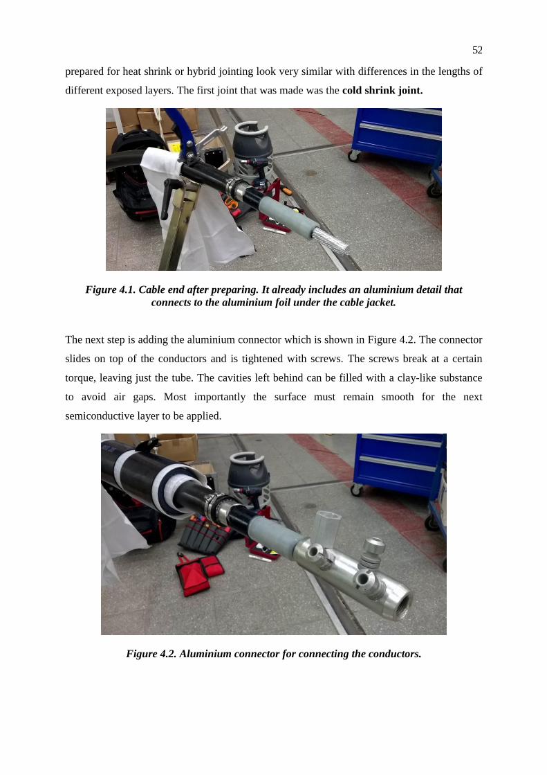
52
prepared for heat shrink or hybrid jointing look very similar with differences in the lengths of
different exposed layers. The first joint that was made was the cold shrink joint.
Figure 4.1. Cable end after preparing. It already includes an aluminium detail that
connects to the aluminium foil under the cable jacket.
The next step is adding the aluminium connector which is shown in Figure 4.2. The connector
slides on top of the conductors and is tightened with screws. The screws break at a certain
torque, leaving just the tube. The cavities left behind can be filled with a clay-like substance
to avoid air gaps. Most importantly the surface must remain smooth for the next
semiconductive layer to be applied.
Figure 4.2. Aluminium connector for connecting the conductors.

53
Along the process thermocouples were inserted into specific layers in order to track the
temperature when current is passed through the cable. An unfinished cable joint with
thermocouples placed inside the conductor, on the connector, on the insulation, on the
aluminium foil under the cable jacket, and on the semiconductor layer is shown in Figure 4.3.
The thermocouples are held in place with insulating tape. There is also a tape layer that makes
the surface of the connector smoother visible in the figure.
Figure 4.3. The unfinished joint with some thermocouples visible.
An important thing to note in these joints is that the presence of the thermocouples greatly
reduces the quality of the joints as the layers cannot be properly sealed and there are more
rough edges. However, since this test only uses currents and no high voltage, these
imperfections should not affect the adequate temperature measurements.
After this stage the joint kit was applied. The middle part is applied. The middle part includes
an aluminium sheath that connects to the aluminium foil layer in the bulk of the cable. The
edge of the middle part with the aluminium sheath connected is shown in Figure 4.4. There
are stress cones built into the joint. The heat shrink joint requires a special tape for this. The
clay strips are meant to block moisture. One of the end pieces that seals the open aluminium
sheath is also visible in the top right of the photo. Before adding the final layer self-
vulcanizing tape is added to insulate the aluminium sheath that is still exposed. Then the final
two components are shrunk onto the ends of the joint that were exposed so far.

54
Figure 4.4. Cold joint sheath connected to the aluminium foil.
The finished cold shrink joint is shown in Figure 4.5. The final piece of tape being applied is
only meant to secure the final thermocouple on the surface of the joint. One more
thermocouple is placed 70 cm from the centre of the joint onto the cable jacket. A small cut
was made into the jacket to place that thermocouple.
Figure 4.5. Finished cold shrink joint.
In making the heat shrink joint an additional layer of stress control tape ( ) was added
on top of the connector. The tape (yellow) is shown in Figure 4.6. The insulating layers are
visible in the photo on the right side. There are two layers because the thickness of each layer
is limited by thermomechanical properties of the material. The innermost black layer is stress

55
control ( ). The next red layer on the outside of the inner tube and the inside of
the outer tube is XLPE insulation ( ). The outer black layer is semiconductive
material for a more homogenous field. The inner layer is called SISCT and the outer layer is
called SIST. So far there are thermocouples on the conductor and connector. Another is added
on the insulation, on the semiconductor, on the inner tube, and on the outer tube.
Figure 4.6. Field control tape on the connector. The insulating tubes (2 layers) are visible
on the right side of the image.
The heat was applied by a blowtorch. Heating should begin from the middle of the joint to
prevent trapping any air inside. After that the two insulating layers were covered by an
aluminium sheath and then finally covered with an additional heat shrinking insulation layer.
The aluminium sheath is shown in Figure 4.7. The final layer being shrunk down with a
blowtorch is shown in Figure 4.8.
Figure 4.7. Aluminium sheath in the joint. The metal rings compress it onto the aluminium
foil in the cable bulk.
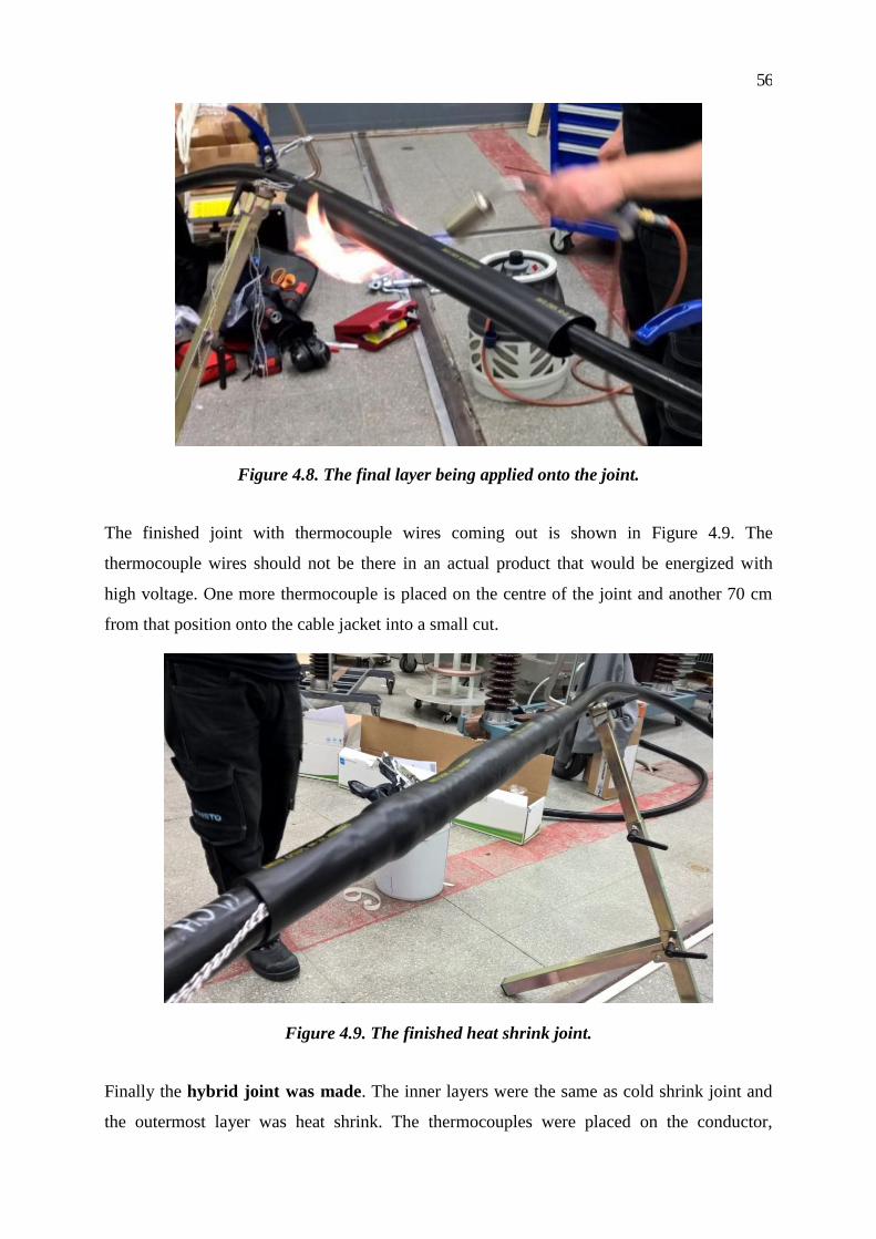
56
Figure 4.8. The final layer being applied onto the joint.
The finished joint with thermocouple wires coming out is shown in Figure 4.9. The
thermocouple wires should not be there in an actual product that would be energized with
high voltage. One more thermocouple is placed on the centre of the joint and another 70 cm
from that position onto the cable jacket into a small cut.
Figure 4.9. The finished heat shrink joint.
Finally the hybrid joint was made. The inner layers were the same as cold shrink joint and
the outermost layer was heat shrink. The thermocouples were placed on the conductor,

57
connector, insulation, semiconductor layer, aluminium foil, on top of the cold shrink layer, on
top of the heat shrink layer (outside the joint), and 70 cm from joint centre on the cable jacket
into a small cut. The hybrid joint being finished by heat shrinking the outermost layer is
shown in Figure 4.10. The metal piece still on the cable is meant to protect the thermocouples
from the heat from the blow torch.
Figure 4.10. The outermost layer of the hybrid joint being heat shrunk.
4.1.2 Measurement Setup
The cable with three joints in it was looped twice through a transformer that induced the
current in it. The aluminium foil in the cable was grounded to prevent inducing any voltages
in it. The transformer was powered by a power source. With 650 A flowing through the cable
the transformer current was 10 A at 130 V, making the power out to be about 1.3 kW (the
angle between the current and the voltage is not known). The current in the cable was
measured with an inductive loop (in the results indicated as “Current (A)”). A thermocouple
was added in the middle of the setup to measure ambient air temperature. That thermocouple
was placed into a jar of oil to increase the time constant for temperature changes and have less
fluctuations from opening and closing the room door. The setup with the cable,
thermocouples, current meter, transformer, and power supply is shown in Figure 4.11.

58
Figure 4.11. The Final test setup.
All thermocouples were connected to a temperature recorder. There were 3 hubs, each for one
joint, with 8 channels in each hub. The ambient temperature sensor was connected to channel
8 in the cold shrink joint hub. The layers in which thermocouples (TC) were placed are shown
in Table 4.1.
Table 4.1. Thermocouples and sensors used in the measurements.
TC0 (heat shrink) TC1 (hybrid joint) TC2 (cold shrink)
Channel Layer Channel Layer Channel Layer 0 Connector 0 Connector 0 Connector 1 Conductor 1 Conductor 1 Conductor 2 XLPE 2 XLPE 2 XLPE
3 Semiconductor 3 Semiconductor 3 Semiconductor 4 SISCT tube 4 Al foil 4 Al foil 5 SIST tube 5 Cold joint
surface 5 Joint surface
6 Joint surface 6 Joint surface 6 Cable jacket 7 Cable jacket 7 Cable jacket 7 Ambient
4.2 Cable Thermal Response to Currents
The temperatures of the cable were tested in two runs. The first was used to find out the
temperatures that correspond to certain current levels in the cable. The second run was done
to see the heating process up to 90˚C more clearly.

59
4.2.1 Run #1
The first run was done at different current levels to determine the currents at which the
conductor reaches a certain temperature. The levels were chosen to be 400 A (supposed to
operate at 65˚C, actually reached 45˚C) and 510 A (supposed to operate at 90˚C, actually
reached 60˚C). The third current level was calculated to be 650 A for operating at 90˚C
(which is the maximum allowed temperature) based on the previous temperatures and
currents. The cable did not reach that temperature in the first run due to lack of testing time.
The datasheet current values were probably conservative to be on the safe side. Also the cable
is normally meant to be in a bundle and that reduces the cooling efficiency compared to the
test setup.
The current value 400 A was applied for 201 minutes, 510 A was applied from 201 minutes
from the start to 360 minutes and 650 A was applied from 360 minutes to 369 minutes. After
that cooling was observed for a longer period and the graphs are non-linear after shutting off
the 650 A current. There was a power interruption due to a short circuit at 350 minutes.
As seen in Figure 4.12, Figure 4.13, and Figure 4.14, the cable layers start to heat
exponentially as current is applied to the cable. There are some seemingly random
fluctuations in the current and temperatures. The current fluctuations are due to the fact that
the current was induced by a voltage source that was connected to the grid. Thus all grid
voltage fluctuations are visible in the results. If the current dropped too much then it was
adjusted. Those adjustments are also visible in the graphs (slight and sudden increases in
current). There are also some temporary drops in the temperature of the outer layers due to
opening the door of the room where the test was set up. The ambient temperature sensor did
not register these drops because it was situated in oil, thus increasing the temperature time
constant. The ambient temperature rises throughout the test since the cable acts as a radiator
in the small room.

60
Figure 4.12. Temperatures in the heat shrink joint in run #1.
Figure 4.13. Temperatures in the hybrid joint in run #1.
0
100
200
300
400
500
600
700
0
10
20
30
40
50
60
70
01
63
24
76
37
99
51
11
12
71
43
15
91
75
19
12
07
22
32
40
25
62
72
28
83
05
32
13
38
35
43
71
38
74
68
69
29
17
11
41
I (A
)
T (˚C
)
t (min)
Connector Conductor XLPE Semicon SISCT
SIST Joint surface Cable jacket Ambient air Current (A)
0
100
200
300
400
500
600
700
0
10
20
30
40
50
60
70
01
63
24
76
37
99
51
11
12
71
43
15
91
75
19
12
07
22
32
40
25
62
72
28
83
05
32
13
38
35
43
71
38
74
68
69
29
17
11
41
I (A
)
T (˚C
)
t (min)
Connector Conductor XLPE Semicon Al foil
CS layer Joint surface Cable jacket Ambient air Current (A)

61
Figure 4.14. Temperatures in the cold shrink joint in run #1.
There are some common traits in all joints. The thermal constant seems to be similar in all
layers since the temperature becomes stable in all layers about 3 hours after the change in
current.
The inner layers reach a much higher temperature than the outer layers. The inner layers
(connector and conductor) are the layers actually producing the heat. The conductor and the
connector are roughly at the same temperature. The connector is slightly cooler. The
difference reaches up to 1.5˚C, but is smaller in general. Although the difference is within the
error of measurement, it is persistent. The difference can be explained by the bigger mass of
the connector.
The cable jacket 70 cm from the centre of the joint heats up and then settles to the balanced
temperature faster than the rest of the cable. This means a reduced thermal time constant. The
reason is probably smaller thickness and mass of insulation on the cable which allows the heat
from the conductor to penetrate to the cable surface faster.
0
100
200
300
400
500
600
700
0
10
20
30
40
50
60
70
80
0
16
33
49
65
82
98
11
5
13
1
14
8
16
41
81
19
8
21
5
23
2
24
8
26
5
28
2
29
9
31
6
33
3
35
0
36
7
38
4
43
8
67
0
90
2
11
35
I (A
)
T (˚C
)
t (min)
Connector Conductor XLPE Semicon Al foil
Count of a Joint surface Cable jacket Ambient air Current (A)

62
There are also differences between different joints. The heat shrink joint is the coolest while
the cold shrink joint is the hottest with the hybrid joint temperature lying in between. This is
probably due to the joint thickness. The heat shrink joint is the slimmest with better cooling
properties while the cold shrink joint has the thickest layer of insulation on top. The thick
layers prevent heat transfer with the ambient environment.
The maximum temperatures that were achieved are shown in Table 4.2 and Table 4.3. The
temperature at 400 A was recorded at 12000 seconds (200 minutes) and the temperature at
510 A was recorded at 21000 seconds (350 minutes).
Table 4.2. Maximum temperatures in different joint layers at 400 A.
TC0 (heat shrink) TC1 (hybrid joint) TC2 (cold shrink) Layer Temp (˚C) Layer Temp (˚C) Layer Temp (˚C) Conductor 42.5 Conductor 44.9 Conductor 45.5 Connector 43.1 Connector 45.3 Connector 45.6
XLPE 38.0 XLPE 41.5 XLPE 41.9 Semiconductor 38.5 Semiconductor 39.4 Semiconductor 39.2 SISCT tube 37.3 Al foil 38.4 Al foil 39.7
SIST tube 36.0 Cold joint surface
36.0
Joint surface 33.0 Joint surface 34.2 Joint surface 33.1 Cable jacket 33.9 Cable jacket 37.6 Cable jacket 37.1 Ambient 23.1 Ambient 23.1 Ambient 23.1
Table 4.3. Maximum temperatures in different joint layers at 510 A.
TC0 (heat shrink) TC1 (hybrid joint) TC2 (cold shrink) Layer Temp (˚C) Layer Temp (˚C) Layer Temp (˚C) Conductor 57.5 Conductor 60.9 Conductor 62.0
Connector 58.5 Connector 61.6 Connector 62.3 XLPE 49.7 XLPE 54.7 XLPE 55.5 Semiconductor 50.6 Semiconductor 50.8 Semiconductor 50.3 SISCT tube 48.3 Al foil 50.1 Al foil 51.3 SIST tube 45.9 Cold joint
surface 46.3
Joint surface 41.4 Joint surface 43.0 Joint surface 41.3 Cable jacket 44.0 Cable jacket 48.2 Cable jacket 46.8 Ambient 23.1 Ambient 23.1 Ambient 23.1
4.2.2 Run #2
In the second run the current was set to 650 A, the expected equilibrium temperature was 90˚
C (rough estimation calculated from the equilibrium temperatures at 400 A and 510 A). The
results are shown in Figure 4.15, Figure 4.16 and Figure 4.17.

63
Figure 4.15. Temperatures in the heat shrink joint in run #2.
Figure 4.16. Temperatures in the hybrid joint in run #2.
0
100
200
300
400
500
600
700
0
10
20
30
40
50
60
70
80
90
0 91
92
83
74
65
66
57
48
49
31
02
11
21
21
13
11
40
15
01
59
16
91
78
18
81
98
20
72
17
22
62
36
24
52
55
26
5
I (A
)
T (˚C
)
t (min)
Connector Conductor XLPE Semicon SISCT
SIST Joint surface Cable jacket Ambient air Current (A)
0
100
200
300
400
500
600
700
0
10
20
30
40
50
60
70
80
90
100
0
10
19
29
38
48
58
67
77
87
96
10
6
11
6
12
6
13
5
14
5
15
5
16
5
17
5
18
5
19
5
20
5
21
5
22
5
23
5
24
5
25
5
26
5
I (A
)
T (˚C
)
t (min)
Connector Conductor XLPE Semicon Al foil
CS layer Joint surface Cable jacket Ambient air Current (A)

64
Figure 4.17. Temperatures in the cold shrink joint in run #2.
The current was applied for 166 minutes and then it was switched off. The current was
switched off because the conductor in the cold shrink joint reached the temperature of 90˚C.
That was not quite the equilibrium temperature but higher temperatures may damage the joint.
However, since the temperature is known to balance out at roughly 3 hours, it is quite close.
The current decreases slightly throughout the test, but is adjusted twice to maintain a value
close to 650 A. The current decrease may be a result of voltage changes on the grid or also
increased conductor resistance due to higher temperature.
The current was applied for 166 minutes until the maximum conductor temperature reached
90˚C. Then cooling was observed for 107 minutes after the current was switched off.
Similarly to the first run the cold shrink joint reached the highest temperature while the heat
shrink joint was the coolest. Also the cable jacket 70 cm from the centre of the joint heated up
and started to reach a stable temperature faster than the layers inside the joints. The cable
jacket also cools down more rapidly.
The cooldown after shutting off the current was observed for 107 minutes. In that time the
temperature dropped from 90.1˚C to 29.6˚C in the cold shrink joint conductor (roughly 60˚C
change). 107 minutes (6420 seconds) after the current was applied the temperature inside the
0
100
200
300
400
500
600
700
0
10
20
30
40
50
60
70
80
90
100
0
10
19
29
38
48
58
67
77
87
96
10
6
11
6
12
6
13
5
14
5
15
5
16
5
17
5
18
5
19
5
20
5
21
5
22
5
23
5
24
5
25
5
26
5
I (A
)
T (˚C
)
t (min)
Connector Conductor XLPE Semicon Al foil
a Joint surface Cable jacket Ambient air Current (A)

65
cold shrink joint conductor had increased to about 82.3˚C from the initial 20.5˚C (roughly 62˚
C change). Considering that at the end the room temperature had increased to 23.5˚C from the
initial 21.3˚C, thus lowering the cooling rate slightly, it is safe to assume that the temperature
change time constant is equal for both heating and cooling, as it theoretically should be.
The maximum temperatures that were achieved are shown in Table 4.4. The temperature was
recorded at 10000 seconds (167 minutes).
Table 4.4. Maximum temperatures in different joint layers at 650 A.
TC0 (heat shrink) TC1 (hybrid joint) TC2 (cold shrink) Layer Temp (˚C) Layer Temp (˚C) Layer Temp (˚C) Conductor 83.6 Conductor 88.1 Conductor 90.1 Connector 82.1 Connector 86.9 Connector 89.5 XLPE 67.5 XLPE 74.9 XLPE 77.1 Semiconductor 69.2 Semiconductor 68.0 Semiconductor 67.2 SISCT tube 64.9 Al foil 67.7 Al foil 69.0 SIST tube 60.7 Cold joint
surface 61.4
Joint surface 53.2 Joint surface 55.9 Joint surface 53.3
Cable jacket 59.7 Cable jacket 65.4 Cable jacket 60.7 Ambient 23.5 Ambient 23.5 Ambient 23.5
The temperature differences in different layers of joints have some similarities. The inner
layers are mostly hotter than the outer layers. The connector and conductor are at similar
temperatures.
There is a bigger drop-off in the XLPE layer (between CH1 and CH2). The temperature
difference is between 13˚C and 16˚C, the highest difference being in the heat shrink joint and
the lowest in the cold shrink joint. Assuming linear temperature drop, the temperature
gradient is as high as 2.9˚C/mm. This means that most of the thermomechanical stress lies in
the XLPE layer. It is unclear how big this issue is, but since XLPE is somewhat flexible and
the temperature differences are not huge, it can be assumed that the thermomechanical
stresses have a much lesser impact than the high temperature.
In the heat shrink joint the outside of the semiconductor layer is hotter than the XLPE layer.
The same is seen at the semiconductor layer and Al foil in the cold shrink joint. That is
probably because the thermocouples are situated at different location on the cable and the
heating may be uneven within the joint.

66
There is also an apparent big drop from the XLPE to the semiconductor layer (between CH2
and CH3) in the cold shrink and hybrid joint. Since the thermocouples are situated apart in the
cable the temperature drop is not necessarily realistic. If the temperature drop were true then
due to the very small thickness of the semiconductor layer the thermal gradient would be
significant.
The temperature drops in other layers apart from XLPE, towards the outside surface of the
cable are smaller. As discussed earlier, the cable jacket surface 70 cm from the joint centre is
hotter than the joint surface. This is because the cable jacket is thinner and allows a higher
rate of heat transfer. It can be assumed that the inner layers and the conductor are at a lower
temperature where the insulation thickness is smaller. This is visible when comparing the
layer temperatures of the thick cold shrink joint to those of the thinner heat shrink and hybrid
joints.
67
Conclusion
The aim of the testing was to reach 90˚C in the hottest layer of the joints. The test was
stopped when the hottest conductor reached 90˚C. The other conductors were at a lower
temperature. According to the cable data sheet the system should be safe to operate at 510 A
and not exceed 90˚C. However, in this test the temperatures barely reached 62˚C at a 510 A
load. The current was increased to 650 A in order to obtain the desired temperature. This
means there is a safety margin of approximately 22%
As expected the inner layers of the cable joint are hotter because that is where the heat
originates. The biggest temperature drop towards the outside of the cable occurs in the XLPE
insulation layer. The temperature on the inside of the XLPE is very close to the conductor
temperature (90˚C) while the outer layer temperature is up to 16˚C lower than that. It is
known that high temperature is a cause of degradation in insulation. The material properties,
more specifically heat expansion coefficient should be studied to determine if the temperature
gradient and the resulting thermomechanical stresses are also an important contributing factor
to insulation degradation.
While the joint surface temperature is similar in all cases, the XLPE temperature and
conductor temperature differ according to joint type. The temperatures of the inner layers are
lower in the heat shrink joint and the XLPE in the cold shrink joint is the first to reach 90˚C.
Since the XLPE layer is the most likely to fail due to high temperatures then heat shrink type
joints are more suitable for operation in conditions where long periods of high loads are
frequent. Also it is apparent that the temperatures reach higher values at joints than they do in
the bulk of the cable. Thus, it is beneficial to keep the number of joints low.
The actual degradation processes in different joint types should be studied further to confirm
that thinner heat shrink joints perform better in highly loaded (like in case of stochastic load
patterns of wind and solar energy plants) cable lines with radial network topology. Also a
larger number of joints should be studied to reduce statistical error and get more reliable data
about the differences between joint types. The aging should be done over a longer period of
time using different load patterns to see the differences in cable degradation speed.
The cable takes some time to get up to final operational temperature whenever current
increases. This means that longer periods of full capacity loading are much more likely to
make the cable reach high temperatures near 90˚C. This is the case with wind farms where the
load depends on the wind conditions and can remain at high values during periods of good

68
wind conditions, whereas the traditional loading pattern has shorter periods of near maximum
capacity current. Thus, wind turbine radial lines are more likely to be subjected to high
temperatures, resulting in an increased degradation rate.
It is clear that the XLPE temperature is higher near the thicker parts of the cable or joints
where the cooling is slower. Further studies should be conducted to find out about how the
temperature changes along the cable length. This could help to rate the currents that the joints
can handle more reliably. It can be assumed from this finding that compact joints with thinner
layer thicknesses may be more suitable than other joint types for wind turbine radial cables
where the cooling of the cable is crucial. However, there may be other important factors that
were not studied in this thesis.
For reduced thermal effects forced cooling possibilities should be looked into. Since the
conductor is hotter in areas with thicker insulation, it can be assumed that the insulation
temperatures are the highest near the joints. Thus, joint temperature is a better indicator of the
operating conditions in the system than the cable bulk temperature. If the conductor
temperature in the bulk of the cable reaches 90˚C then the joint temperature is probably
already higher. For practical purposes this means that local cooling near joints may be
sufficient to increase the system current rating and reliability.
For future studies the placement of thermocouples can be improved in terms of distance
between the thermocouples along the cable to give more reliable results. The electrical
resistance of the conductor connections in the joints was not measured in this testing as it
should be in order to make sure the temperature differences don’t arise from variations in joint
electrical connection quality instead of joint type. Instead of a voltage source a current source
should be used for a more stable supply independent of the grid voltage fluctuations. The
effect of the electrical field can be studied by applying voltage to the system. The room
temperature can be controlled a bit more closely for more precise results, although that effect
is negligible with the accuracy level of this test.

69
References
[1] Elektrilevi OÜ, “Majandusaasta aruanne 2013,” Tallinn, 2014.
[2] M. Abdel-Salam, H. Anis, A. El-Morshedy and R. Radwan, High-Voltage Engineering,
New York, 2000.
[3] M. Meldorf, J. Kilter, H. Tammoja and Ü. Treufeldt, Jaotusvõrgud, Tallinn, 2007.
[4] J. Hansen, “Failures in MV Joints (XLPE Cables) in Heavily Loaded Cable Systems
Connecting Large Wind Turbines to the Distribution System,” Espoo, 2012.
[5] S. Chaitusaney and P. Pongthippitak, “Integration of Battery for Attenuating Frequency
Fluctuation due to Wind Turbine Generation,” Chulalongkorn University, 2009.
[6] I. Kiitam, Methods For Testing the Insulation of Power Cables, Tallinn: Tallinn
University of Technology, 2014.
[7] BICC Cables, Electric Cables Handbook, Third Edition, Blackwell Publishing, 2006.
[8] Indonetwork, “indonetwork.net,” [Online]. Available:
http://202.67.224.137/pdimage/25/4404025_cables.jpg. [Accessed 2015].
[9] P. Taklaja, “Harku-Lihula-Sindi 330kV/110kV õhuliin versus kaabelliin,” Tallinn, 2013.
[10] B. S. Bernstein, “Electrical Properties of Cable Insulation materials,” 2001. [Online].
Available:
http://www.pesicc.org/iccwebsite/subcommittees/E/E04/2001/f2001_bernstein.pdf.
[Accessed 2014].
[11] P. Hyvönen, “Prediction Of Insulation Degradation Of Distribution Power Cables Based
On Chemical Analysis And Electrical Measurements,” Espoo, 2008.
[12] W. Choo, G. Chen and S. G. Swingler, “Electric Field in Polymeric Cable due to Space
Charge Accumulation under DC and Temperature Gradient,” Southampton, 2011.
[13] Eesti Standardikeskus, EVS-EN 60228:2005, 2005.
[14] Eesti Standardikeskus, EVS-EN 1715-2:2008, 2008.

70
[15] Eesti Standardikeskus, EVS-EN 50356:2003, 2003.
[16] J. Kaumanns, “The Skolkovo challenge: A 550 kV XLPE cable system with 138 joints
put into operation within 17 month after order intake,” 2012. [Online]. Available:
www.cigre.org/content/download/26192/1129889/version. [Accessed 2014].
[17] Prysmian Group, “Western HVDC Link,” Prysmian Group, 2013. [Online]. Available:
http://prysmiangroup.com/en/corporate/about/special_projects/western-HVDC-link/.
[Accessed 2014].
[18] Eesti Standardikeskus, EVS-IEC 60364-4-42:2003, 2003.
[19] S. McFayden, “Cable Sheath and Armour Loss,” 2013. [Online]. Available:
http://myelectrical.com/notes/entryid/235/cable-sheath-and-armour-loss. [Accessed
2015].
[20] HyperPhysics, “Dielectrics,” [Online]. Available: http://hyperphysics.phy-
astr.gsu.edu/hbase/electric/dielec.html. [Accessed 2014].
[21] Eesti Statistikaamet, EVS-EN 50397-2:2009, 2009.
[22] Ensto, “CJAIO11.2403C-ALS Cold shrink joint,” [Online]. Available:
http://products.ensto.com/catalog/22453/product/45446/CJAIO11.2403C-
ALS_ENG1.html. [Accessed 2015].
[23] Campbell White, “Cable Jointing-Splicing companies Australia,” [Online]. Available:
http://www.campbellwhite.com/CJ_History.aspx. [Accessed 2015].
[24] A. Kuusik, “Kuni 24 kV sise- ja välisotsamuhvidest 2,” Elektriala, no. 2, pp. 18-19,
2015.
[25] L. Dissado and J. Fothergill, Electrical Degradation and Breakdown in Polymers,
London: Peter Peregrinus Ltd., 1992.
[26] Industrial High Voltage, Delft: Delft University Press, 1991.
[27] J. Niitsoo, I. Palu, J. Kilter, P. Taklaja and T. Vaimann, “Residential Load Harmonics in
Distribution Grid,” in 3rd International Conference on Electric Power and Energy
Conversion Systems, Istanbul, 2013.

71
[28] P. Tani, Insulation Condition Assessment Using the Time-Resistance Test, Tallinn:
Tallinn University of Technology, 2014.
[29] A. Babaee and S. M. Shahrtash, “Partial Discharge Propagation in Cable with
Semiconductor Layer,” in Electrical Insulation and Dielectric Phenomena (CEIDP),
2012.
[30] P. Hyvönen, “Aine "Liigpinged" konspekt,” 2014.
[31] Eesti Standardikeskus, EVS-EN 6081-1-2:2001, 2001.
[32] Wikipedia, “Thermal contact conductance,” [Online]. Available:
http://en.wikipedia.org/wiki/Thermal_contact_conductance. [Accessed 2015].
[33] J. Luo, Z. Li and Y. Liu, “Study on the thermal expansion of EHV cable line with large
size conductor in tunnel,” in Transmission and Distribution Conference and Exposition,
2010 IEEE PES , 2010.
[34] J. T. Holboll, M. Henriksen and J. Hjerrild, “Conference on Electrical Insulation and
Dielectric Phenomena,” in Space Charge Build-up in XLPE-Cable with Temperature
Gradient, 2000.
[35] F. N. Lim and R. J. Fleming, “Conference on Electrical Insulation and Dielectric
Phenomena,” in The Temperature Dependence of Space Charge Accumulation and DC
Current in XLPE Power Cable Insulation, 1999.
[36] F. Viola and P. Romano, “Building Partial Discharge Signal Wireless Probes,” 2014.
[Online]. Available: http://www.intechopen.com/books/progress-in-compact-
antennas/building-partial-discharge-signal-wireless-probes. [Accessed 2015].
[37] Ensto Hybrid joint, “CJWH11.2403C,” [Online]. Available:
http://products.ensto.com/catalog/21434/product/30696/CJWH11.2403C_ENG1.html.
[Accessed 2015].
[38] Ensto, “HJW11.2403C Heat shrink joint,” [Online]. Available:
http://products.ensto.com/catalog/21316/product/15853/HJW11.2403C_ENG1.html.
[Accessed 2015].