Temperature and Growth:A Panel Analysis of the United States

Riccardo Colacito Bridget Hoffmann Toan Phan∗

————————————————————————————————————–

Abstract

We document that seasonal temperatures have significant and systematic effectson the U.S. economy, both at the aggregate level and across a wide cross-section ofeconomic sectors. This effect is particularly strong for the summer: a 1oF increase inthe average summer temperature is associated with a reduction in the annual growthrate of state-level output of 0.15 to 0.25 percentage points. We combine our estimateswith projected increases in seasonal temperatures and find that rising temperaturescould reduce U.S. economic growth by up to one-third over the next century.

JEL classification: O44; Q51; Q59; R11.This draft: March 30, 2018.

————————————————————————————————————–

∗Colacito is affiliated with the Kenan-Flagler Business School and the Department of Economics atthe University of North Carolina at Chapel Hill. Hoffmann is affiliated with the Research Departmentat Inter-American Development Bank. Phan is affiliated with the Federal Reserve Bank of Richmond.Emails: ric@unc.edu, bridgeth@iadb.org, and toanvphan@gmail.com. The authors acknowledgehelpful comments from the editor and two anonymous referees, as well as helpful discussions with RaviBansal, Marshall Burke, Tatyana Deryugina, Don Fullerton, Duane Griffin, Solomon Hsiang, BenjaminJones, Ju Hyun Kim, and Mike Roberts. We also thank conference/seminar participants at the AmericanEconomic Association, Econometric Society World Congress, Association of Environmental and ResourceEconomists, European Economic Association Annual Congress, Triangle Resource and EnvironmentalEconomics, University of Illinois at Chicago, UNC–Chapel Hill, and University of Hawaii. The viewsexpressed herein are those of the authors and not those of the Federal Reserve Bank of Richmond orthe Federal Reserve System, or the Inter-American Development Bank, its Board of Directors, or thecountries they represent. All errors are ours.

Working Paper No. 18-09

1 Introduction

We analyze the effect of average seasonal temperatures on the growth rate of U.S. out-

put. We find that seasonal temperatures, particularly summer temperatures, have sig-

nificant and systematic effects on the U.S. economy, both at the aggregate level and

across a wide cross-section of economic sectors. A 1oF increase in the average summer

temperature is associated with a reduction in the annual growth rate of state-level out-

put of 0.15 to 0.25 percentage points.

As global average temperatures are predicted to continue rising over this century, many

scholars and policymakers have raised warnings of the potential for dramatic damages

to the global economy (e.g., Stern (2007), Field et al. (2014)). The economics literature

has documented substantial negative effects of global warming on economic growth in

developing economies (e.g., Gallup, Sachs and Mellinger (1999), Nordhaus (2006), Burke

et al. (2009), Dell, Jones and Olken (2012)). For the U.S., however, it has been challeng-

ing to provide systematic evidence that rising temperatures affect the growth rate of

economic activities beyond sectors that are naturally exposed to outdoor weather condi-

tions (see Mendelsohn and Neumann (1999), Schlenker and Roberts (2006; 2009), and

Burke and Emerick (2015) for an analysis of an agricultural industry). We contribute to

this literature by providing comprehensive evidence that rising temperatures do affect

U.S. economic activities, at both the aggregate and industry levels.

We overcome existing challenges by exploiting random fluctuations in seasonal temper-

atures across years and states. Using a panel regression framework with the growth

rate of state GDP, or gross state product (henceforth GSP), and average seasonal tem-

peratures of each U.S. state, we find that summer and fall temperatures have opposite

effects on economic growth. An increase in the average summer temperature negatively

affects the growth rate of GSP, while an increase in the fall temperature positively af-

fects this growth rate, although to a lesser extent. The different signs of the two effects

1

suggest that previous studies’ aggregation of temperature data into annual tempera-

ture averages (e.g., Dell et al. (2012)) may mask the heterogeneous effects of different

seasons.

The summer effect dominates the fall effect in our recent sample (post-1990), leading to

a negative net economic effect of rising temperatures. This implies that the U.S. econ-

omy is still sensitive to temperature increases, despite the progressive adoption of adap-

tive technologies such as air conditioning (Barreca et al. (2015)). We also document that

the temperature effects are particularly strong in states with relatively higher summer

temperatures, most of which are located in the South. However, we do not find any evi-

dence that the effect of temperature on GDP in the South is driven by the relatively less

developed states. This implies that the channel through which temperature affects GDP

in this part of the country must be distinct from the one documented in the literature

for developing economies.

We revisit the conjecture that only a small fraction of the sectors of the economy are

sensitive to rising temperatures in developed economies, implying that the aggregate

economic impact of warming on the U.S. will be limited (Schelling (1992), Mendelsohn

(2010), Nordhaus (2014)). Our results show that rising summer temperatures have a

pervasive effect in the entire cross-section of industries, above and beyond the sectors

that are traditionally deemed as vulnerable to changing climatic conditions. Figure 1

documents that, in the most recent part of our sample, an increase in the average sum-

mer temperature negatively affects the growth rate of output of many industries, includ-

ing finance, services, retail, wholesale, and construction, which in total account for more

than a third of national gross domestic product (GDP). Only a limited number of sec-

tors, such as utilities (1.8% of national GDP), which includes providers of energy, benefit

from an increase in the average summer temperature.1 To the best of our knowledge,

our paper is the first in the literature to systematically document the pervasive effect of1Section 4.2 provides a comprehensive break-down of these results across different samples and sub-

industries.

2

Fin

ance

,R

eal E

stat

e,an

d In

sura

nce

Ser

vice

s

Agr

icul

ture

Who

lesa

le

Con

stru

ctio

n

Ret

ail

Com

mun

icat

ion

Gov

erne

men

t

Tra

nspo

rtat

ion

Man

ufac

turin

g

Util

ities

Min

ing

-0.25

-0.2

-0.15

-0.1

-0.05

0

0.05

0.1

0.15

Effe

ct o

f Sum

mer

Tem

pera

ture

on

GD

P ti

mes

Indu

stry

Sha

re

All Industries = -0.256 (0.060)

Figure 1: Decomposition of the Summer temperature effect in the cross-section of industries.For each industry, the horizontal line represents the point estimate of the impact of Summertemperature on the growth rate of industry GDP times the industry share of GDP. The bottomand top portions of each rectangle represent 90% confidence intervals, while the outer limitsof each boxplot represent the 95% confidence interval of each estimated coefficient. Standarderrors are clustered at the year level. The number denoted as “All Industries” is the sum of allthe industry coefficients multiplied by the corresponding industry share. All estimates refer tothe post-1997 sample as documented in Table 4A of Section 4.2.

summer temperatures on the cross-section of industries in the U.S..

We document that temperature may affect economic activities through its impact on

labor productivity. In our empirical analysis, an increase in the average summer tem-

perature decreases the annual growth rate of labor productivity, while an increase in

the average fall temperature has the opposite effect. While our finding sheds light on

the effects of temperature on labor productivity at the macroeconomic level, it is also

3

consistent with existing studies of this relationship at the microeconomic level. For

example, Zivin and Neidell (2014) have found that warmer temperatures reduce labor

supply in the U.S., and Cachon, Gallino and Olivares (2012) have documented that high

temperatures decrease productivity and performance.

Our paper also contributes to the growing debate on the long-term economic conse-

quences of rising global temperatures (e.g., Mendelsohn and Neumann (1999) and Tol

(2010)). We combine our estimates of the effects of seasonal temperatures on the growth

rate of U.S. output with several projections of the expected U.S. temperature change

over the next century. We conduct our analysis under a “business as usual” benchmark,

in which there is no additional mitigation and the estimated effects of temperature on

economic growth remain unchanged over the long horizon. We document that the pro-

jected increases in summer and fall temperatures could reduce the growth rate of annual

nominal GDP by up to 1.2 percentage points, which is roughly a third of the historical

average nominal growth rate of about 4% per year.

Our analysis highlights the complex ways in which temperatures affect economic activ-

ities, and it reveals the need to disaggregate the data into seasons and industries to

uncover the full extent of this impact. By providing specific estimates of the effect of

temperature on economic activities in the U.S., our empirical analysis informs a grow-

ing body of literature focused on general equilibrium models of climate change, including

integrated assessment models. These models constitute the basis of many policy recom-

mendations regarding the regulation of greenhouse gas emissions (e.g., Golosov et al.

(2014), Acemoglu et al. (2012), Bansal and Ochoa (2011), and Bansal, Ochoa and Kiku

(2014)). All of these models critically rely on empirical estimates of the impacts of rising

temperatures on aggregate economic activities. In the absence of specific estimates for

the U.S., the parameters of these “climate damage functions” are generally calibrated to

match cross-country estimates (e.g., Nordhaus and Sztorc (2013)). In this respect, our

analysis helps bridge the gap between the theoretical and empirical literatures and will

4

enable researchers to sharpen the policy recommendations based on this class of models,

especially for the U.S.

Our focus on quarterly temperature fluctuations allows us to combine our estimates

with existing climatological projections, which are typically only available at lower fre-

quencies. Our analysis differs from a large literature that uses daily temperature fluctu-

ations to study outcomes as diverse as agriculture, local income, birth weight, mortality,

and time allocation (Schlenker and Roberts (2006), Deschenes and Greenstone (2007),

Deryugina and Hsiang (2014), Deschenes, Greenstone and Guryan (2009), Deschenes

and Greenstone (2011), and Zivin and Neidell (2014)). Whereas studies using high fre-

quency data typically focus on the effect of a change in the observed distribution of daily

temperature, we focus on the effect of a change in the mean seasonal temperature.

In a similar vein, Bloesch and Gourio (2015) analyze the impact of temperature and

snowfall during the coldest months of the year (November through March) on the growth

rate of quarterly economic activities. They find that snowfall has a negative effect on

some routinely employed economic indicators such as nonfarm payroll, housing permits,

and housing starts. Our analysis is broadly consistent with their results, which sug-

gests that a drop in temperatures in cold weather seems to have a negative impact on

economic activities. While they focus on the quarter-to-quarter effect of temperature

on economic activity to measure a potential bounce-back effect following adverse winter

weather conditions, we assess the cumulative effect on the annual growth rate of output

and emphasize the effect of summer temperatures.

The rest of the paper is organized as follows. Section 2 provides a description of the

main datasets that we employ in our analysis. Section 3 describes our main results and

documents the stability of the estimated effects over time. Section 4 documents several

economic mechanisms driving the main results, including the effect of temperature on

labor productivity, on the growth rate of output in the cross-section of industries, and in

the cross-section of U.S. regions. Section 5 analyzes the long-term consequences of global

5

warming for the aggregate U.S. economy, in addition to providing robustness checks of

our main results. Section 6 concludes. The Online Appendix provides a comprehensive

set of robustness exercises.

2 Data

This section describes our data sources and the procedures we use to aggregate weather-

related data. We refer the reader to the appendix for additional details.

2.1 Weather data

We use daily station-level weather data from the National Oceanic and Atmospheric

Administration (NOAA) Northeast Regional Climate Center. This dataset contains daily

observations on average temperature, precipitation, and snowfall across U.S. weather

stations. Throughout the paper, the unit of temperature is degrees Fahrenheit. The

longest common sample across all weather stations starts in 1869 and ends in 2012.

In this study, we focus on the 1957–2012 sample, which coincides with the period for

which we have data on GSP (see below). For each weather station, we deseasonalize

the raw data by regressing daily observations on 12 dummies representing the months

of the year and subtract the corresponding estimated monthly component from each

observation (see appendix A.2.1 for details on deseasonalization).2

We aggregate daily weather observations to quarterly averages by taking the average of

the daily observations in each season. We define the winter as January through March,

the spring as April through June, the summer as July through September, and the fall2We have followed the common practice in the macroeconomics literature of not correcting the standard

errors of our analysis to account for the deseasonalization. However, we provide a robustness check of ourresults using a data set which does not seasonally adjust temperatures.

6

as October through December. Our definition of seasons coincides with the definition of

quarters commonly encountered in the macroeconomics literature, and thus will allow

our analysis to contribute to future developments of macroeconomic models that include

climate-related variables. We analyze average seasonal temperatures in order to es-

tablish a connection between long-term temperature changes and economic activities.

This connection can be more accurately assessed using a lower-frequency temperature

measure. We also consider alternative definitions of seasons in the robustness checks in

section 5.3.

To aggregate weather data from the station level to the county and state level, we em-

ploy ArcGIS, a geographic information system, to obtain the coordinates for the centroid

of each of the 3,144 counties and county equivalents, as well as each weather station.

The country, state, and county borders used in ArcGIS are from 2013 topographically

integrated geographic encoding and referencing (TIGER) shape files. These shape files,

along with the area and population of each county are obtained from the U.S. Census

Bureau. We then follow a standard aggregation method (e.g., Deschenes and Greenstone

(2012)). For each county we weight the daily temperature, precipitation, and snowfall

of each weather station in a 500 km radius of the county’s centroid by the inverse of

the straight-line distance between the station and the county centroid. In this way,

the closest weather stations are assigned a larger weight in determining each county’s

weather.

Finally, to aggregate to the state level, we weight the weather observations of each

county in a state in proportion to either the corresponding county’s area or population.

Weighting by area assigns larger weights to larger counties, while weighting by popu-

lation assigns larger weights to more densely populated areas. We use area weights in

the main analysis in the text, but our results are very similar across different weighting

schemes (see section 5.3 and appendix A.6.2). We aggregate state-level weather data to

the country level by following the same procedure.

7

In section 5.3, we document that our results are robust to using non-deseasonalized

gridded temperature data. We use the NOAA U.S. Climate Divisions’ nClimDiv dataset,

which provides absolute monthly temperature averages for each state, derived from

area-weighted averages of 5km × 5km grid-point temperature estimates interpolated

from station data.3 In appendix A.6.1, we replicate all of our results by using gridded

temperature data from the NOAA nClimDiv data set. We show that our results are

robust to the use of this alternative dataset.

2.2 State-level economic data

We use data on nominal GSP between 1957 and 2012 for all 50 states and the District

of Columbia. GSP is defined as the value added in production by the labor and capital

of all industries located in that state. Data for 1957–1962 come from the U.S. Census

Bureau Bicentennial Edition, and data for the 1963–2012 sample come from the U.S.

Department of Commerce’s Bureau of Economic Analysis (BEA). The data frequency

is annual. From the BEA, we also collected data for national GDP, nominal GSP per

capita, real GSP, and industry output data for the 1963–2011 sample. Industry data

for 1963–1997 are categorized using the Standard Industrial Classification (SIC) codes,

while data for 1997–2011 follow the North American Industry Classification System

(NAICS). Finally, annual employment data at the state level (measured in thousands of

employees) are collected from the Bureau of Labor and Statistics for the sample 1990–

2012.3See ftp://ftp.ncdc.noaa.gov/pub/data/cirs/climdiv/climdiv-inv-readme.txt for

more details.

8

3 Main results

In this section we report our main empirical results. First, as a benchmark, we show

that the relationship between temperatures and growth is not statistically significant in

time-series regressions at the whole-country level, consistent with findings in the exist-

ing literature. Then, we improve the analysis by using panel regressions with weather

and economic data from all 50 states plus the District of Columbia (henceforth “the

cross-section of states”).

For the baseline specifications that we consider, we always include the lagged dependent

variable and the average seasonal temperatures. We motivate the inclusion of lagged

GDP growth rates with the strong empirical evidence supporting the claim of first order

auto-correlation of this variable in the cross-section of U.S. states (see table A5 in the

appendix for a complete set of estimates).4 Furthermore, we document in table A6 in

the appendix that the correlation of seasonal temperatures is typically very low. This

supports the claim that our results are unlikely to be affected by multicollinearity.

Our main findings are as follows: (1) an increase in the average summer temperature

negatively affects the growth rate of GSP, and (2) an increase in the average fall temper-

ature positively affects growth, although to a lesser extent. Both effects are statistically

and economically significant. In section 5.3, we perform a comprehensive set of robust-

ness checks and show that the summer effect is generally very robust, while the fall

effect is less so.

Our finding on the compositional effect of seasonal temperatures on GDP is relevant

because it implies that temperature fluctuations may also affect the volatility of GDP

growth. Indeed, given the modest degree of correlation of seasonal temperatures (see ta-

ble A6 in the appendix), our results indicate that temperature’s volatility will contribute4A common concern about including lagged dependent variables in our regressions is that this could

give rise to the Nickell (1981) bias. We show in section 5.3 that our results are robust to excluding thelagged dependent variable.

9

Table 1: Main results:Effects of annual and seasonal temperatures on GSP growth

Whole Year Winter Spring Summer FallTime Series −0.396 −0.071 −0.027 −0.414 0.042

(0.382) (0.179) (0.334) (0.385) (0.287)

Panel Analysis 0.006 0.001 0.003 −0.154 0.102(0.111) (0.049) (0.065) (0.072)∗∗ (0.055)∗

(0.069) (0.025) (0.032) (0.047)∗∗∗ (0.040)∗∗∗

(0.105) (0.044) (0.051) (0.065)∗∗ (0.054)∗

Notes: The first column reports the estimated coefficients on average annual temperature froma regression of the economic growth rate on its lag and the average annual temperature (regres-sions (1) and (3)). The four columns on the right report the estimated coefficients for each ofthe four seasonal temperature averages (regressions (2) and (4)). The top panel (“Time Series”)reports the estimated coefficients using GDP and weather data aggregated to the national level(regressions (1) and (2)). The bottom panel (“Panel Analysis”) reports estimated coefficients us-ing state-level GSP and weather data (regressions (3) and (4)). In the panel regressions, all 50states and the District of Columbia are included and each state is weighted by the proportion,averaged over the whole sample, of its GSP relative to the national GDP. All specifications in-clude the lagged dependent variable, and the panel specifications include state and year fixedeffects. Temperatures are in degrees Fahrenheit. The sample is 1957–2012. Standard errors arein parentheses. In the bottom panel, the standard errors are clustered by year, by state, and byboth dimensions. ***, **, and * denote significance at the 1%, 5%, and 10% levels.

to GDP volatility. This is an important result in light of an abundant macro literature

on the welfare costs of economic fluctuations. This literature, which was started by Lu-

cas (1987), is interested in the question of how much would economic agents be willing

to pay in order to eliminate all sources of fluctuations in business cycles. Equivalently,

if temperature does contribute to business cycle fluctuations, then our analysis is rel-

evant because it points out that there are welfare consequences associated with large

temperature variations.

10

3.1 Benchmark: Time-series regressions with country-level data

We consider two time-series regressions. The first is a regression of the aggregate

growth rate of national GDP on the average annual temperature:

∆yt = βTt + ρ∆yt−1 + α + εt, (1)

where ∆yt denotes the growth rate of national GDP between years t−1 and t; Tt denotes

the annual average temperature in year t in degrees Fahrenheit; and the lagged growth

rate ∆yt−1 controls for autocorrelation.

The second is a regression of the growth rate of aggregate GDP on the average temper-

atures of the four seasons:

∆yt =∑s∈S

βsTs,t + ρ∆yt−1 + α + εt, (2)

where Ts,t denotes the average temperature in season s ∈ S = {winter, spring, summer, fall}

in year t.

The first row of table 1 reports the results of these regressions. The column “Whole

Year” reports the estimate for the coefficient β in equation (1). The remaining columns

report the estimations for coefficients βs in equation (2). As the table shows, none of the

estimated coefficients are statistically significant. These results confirm the difficulty of

identifying the effect of temperature on economic growth in the U.S. documented in the

extant literature.

3.2 Panel regressions with state-level data

We explore the impact of temperature on the growth rates of GSP in the cross-section of

states using two panel specifications that mirror our time-series analysis. The first is a

11

regression of the growth rate of GSP on the state-level annual average temperature:

∆yi,t = βTi,t + ρ∆yi,t−1 + αi+αt+εi,t, (3)

where ∆yi,t and Ti,t denote GSP growth and the annual average temperature in state i in

year t, respectively, while αi and αt denote state and year fixed effects. We again include

the lagged GSP growth rate as a control to capture the degree of autocorrelation of the

dependent variable.

In the second specification, which is the main specification of the paper, we disaggregate

the annual average temperature into four average seasonal temperatures:

∆yi,t =∑s∈S

βsTi,s,t + ρ∆yi,t−1+αi+αt+εi,t, (4)

where the variables are defined as above and Ti,s,t denotes the temperature in degrees

Fahrenheit in state i, year t, and season s. We show in section A.6.4 of the appendix that

our results are robust to using the Arellano and Bond (1991) estimation methodology.

Since some states have larger GSPs and thus contribute more to national GDP than

others, in both panel specifications we weight each state by the proportion of its GSP

relative to the entire country’s GDP over the whole sample (see appendix A.2.2 for de-

tails). In section 5.3 we conduct robustness checks with alternative weighting schemes.

We report the results of these panel regressions in table 1. The column “Whole Year”

refers to the specification in equation (3). We report the estimated coefficient for β

and standard errors. The results indicate that the effect of average temperature at the

annual level is again not statistically significant, confirming the findings in the time-

series specifications.

However, when we break down annual temperatures into the four seasonal tempera-

tures, the results change substantially. The rightmost four columns of table 1 report

12

the estimates for the βs seasonal coefficients with associated standard errors, clustered

by year, by state, and in both dimensions. The table shows the relationship between

average summer and fall temperatures and economic growth rates. These effects are

both statistically and economically significant: a 1oF increase in the average summer

temperature is associated with a reduction in the annual GSP growth rate by 0.154 per-

centage points, while a 1oF increase in the average fall temperature is associated with

an increase in the annual GSP growth rate by 0.102 percentage points.5

The opposite signs of the effects of summer and fall temperatures on GSP growth rates

may partially explain the difficulty of obtaining statistically significant estimates us-

ing annual temperatures. Even though the magnitudes of the summer and fall effects

are comparable, we document through robustness checks (section 5.3) and the exercise

below that the summer effect is much more robust than the fall effect.

3.3 Growth vs. level effects

We test whether the response of GSP to temperature in the previous section is an effect

on the level of output or on its growth rate. It is important to distinguish between these

two hypotheses, because the effects on the growth rate compound over time and thus are

more quantitatively important than effects on the level of output (Pindyck (2011; 2013),

Dell et al. (2012)).

To illustrate the quantitative significance of growth effects compared to level effects, and

to set the stage for our empirical methodology, consider the following simple example.

Assume that the aggregate output of a certain state follows the process:

yt = α + yt−1 + βTt + βlagTt−1 + εt, (5)5We note that the time series point estimates for the summer are larger than the corresponding panel

coefficients, but they are statistically insignificant. This means that by using state level data we obtainan increase in precision due to the increased ability to connect temperatures to local economic variables.

13

where β and βlag denote the impacts of current and lagged average temperatures T (of,

for instance, the current and last summer) on output growth. For simplicity, we assume

that εt = 0, ∀t. Consider a shock in year t = 1 that permanently increases the average

temperature T by one degree Fahrenheit, from T0 = 0 to Tt = 1,∀t ≥ 1 (illustrated in the

left panel of figure 2). This temperature path is motivated by climatologists’ predictions

that temperatures will rise permanently by the middle and end of this century (see

section 5.2 for details). Along this hypothetical temperature path, the level and the

growth rate of output would be

yt = (y0 + β) + (t− 1) [α + (β + βlag)] , and (6)

∆y1 = α + β, and ∆yt = α + (β + βlag) , ∀t ≥ 2, (7)

respectively. We consider three cases. If β = βlag = 0, then temperatures have no

economic effect. We refer to this situation as the No Effect case. If β + βlag = 0, then an

increase in temperature has a permanent impact on the level of output (see equation (6)),

but it affects the growth rate of output for only one period (see equation (7)). We refer to

this situation as the Level Effect case. If β + βlag 6= 0, temperature permanently affects

both the level and the growth rate of output. We refer to this situation as the Growth

Effect case.

We illustrate these three scenarios in the right panel of figure 2. Over the span of 50

years, if temperatures permanently affect the growth rate of output (the Growth Effect

case), then the level of output would be substantially lower than what it would be in

the No Effect case (dashed-dot vs. dashed line). This is in sharp contrast to the case in

which temperature has a permanent effect only on the level of output (the Level Effect

case). In this scenario, after 50 years output is only marginally lower compared to the

baseline case (solid vs. dashed line).

We follow the logic of this example to test whether average seasonal temperatures affect

14

0

10

20

30

40

50

60

70

80

90

100

0 10 20 30 40 50

OUTP

UT

TIME

No Effect

Level Effect

Growth Effect0

0.2

0.4

0.6

0.8

1

1.2

0 10 20 30 40 50

TEMPE

RATU

RE

TIME

Figure 2: Growth vs. level effect. The left panel depicts a permanent increase of 1 degreeFahrenheit in the level of temperature that takes place at year 1. The right panel shows thelevels of output associated with the temperature path reported in the left panel. The three linesare constructed according to equation (5), by setting β = βlag = 0 (dashed line), β = −βlag =

−0.170 (solid line), and β = −0.170, βlag = −0.153 (dash-dot line). In all three cases µ = 2 andεt = 0, ∀t.

the growth rate of GSP in the data. Specifically, we estimate the following equation:

∆yi,t =∑s∈S

βsTi,s,t +∑s∈S

βlag,sTi,s,t−1︸ ︷︷ ︸lagged terms

+ρ∆yi,t−1 + αi + αt + εi,t. (8)

Then we test whether we can reject the null hypothesis that the sum of the contempora-

neous and lagged coefficients for each season is equal to zero, that is, H0 : βs + βlag,s = 0,

for each season s.6

Our results, reported in table 2, indicate that lagged temperatures are generally statis-

tically significant, with the exception of the winter season. The signs of the effects for

summer and fall do not change when considering the lagged temperatures. Most impor-

tantly, from the p-values of the Wald tests reported on the last row of the table, we can

strongly reject the null hypothesis that the sums of the contemporaneous and lagged

temperature coefficients are equal to zero (βs + βlag,s = 0) for summer and fall. This6Note that by setting βs ≡ β/4, βlag,s ≡ βlag/4, for each season s, we obtain the specification for average

annual temperature in (3) augmented with lagged temperature. We omit this case from our investigation,since we did not find any statistically significant effect associated with annual temperatures in table 1.

15

Table 2: Growth vs. level effects

Winter Spring Summer FallContemporaneous temp. −0.008 −0.012 −0.170 0.108

(0.051) (0.059) (0.076)∗∗ (0.050)∗∗

(0.029) (0.032) (0.045)∗∗∗ (0.038)∗∗∗

(0.048) (0.046) (0.067)∗∗ (0.048)∗∗

One-year lagged temp. 0.004 0.121 −0.153 0.066(0.053) (0.063)∗ (0.079)∗ (0.060)(0.023) (0.039)∗∗∗ (0.053)∗∗∗ (0.029)∗∗

(0.046) (0.054)∗∗ (0.075)∗∗ (0.049)

Sum of coefficients −0.004 0.109 −0.323 0.174(0.084) (0.086) (0.115)∗∗∗ (0.077)∗∗

(0.031) (0.045)∗∗ (0.077)∗∗∗ (0.052)∗∗∗

(0.075) (0.068) (0.108)∗∗∗ (0.067)∗∗∗

Wald test’s p-value [0.961] [0.208] [0.007] [0.027][0.893] [0.018] [0.000] [0.002][0.956] [0.110] [0.003] [0.009]

Notes: This table reports results of the growth vs. level regression (8). The first row (“Contempo-raneous temp.”) reports estimates for coefficient β of the effect of contemporaneous temperatureon economic growth, while the second row (“One-year lagged temp.”) reports estimates for coef-ficient βlag of the effects of one-year lagged temperature. The third row (“Sum of coefficients”)reports the sum of β and βlag. The last row (“Wald test p-value”) reports the p-values for theWald test of whether β + βlag is significantly different from zero. Temperatures are in degreesFahrenheit. The sample is 1957–2012. The regressions are weighted by constant GSP shares.The standard errors, clustered by year, by state, and by both dimensions, are in parentheses.***, **, and * denote significance at the 1%, 5%, and 10% levels.

evidence supports the hypothesis that increases in summer and fall temperatures have

lasting effects on output growth. Table A4 in the appendix provides several robustness

checks for the result reported in table 2.

In what follows, we will focus primarily on an econometric specification that omits

lagged temperatures for parsimony. While this results in a bias in our estimated co-

efficients, we note that such bias affects primarily the estimate of the autoregressive

coefficient, and only marginally the estimated temperature coefficients (as can be noted

by comparing tables 1 and 2). For completeness the robustness of all the results of our

subsequent analysis including lagged temperatures are reported in section A.6.3 of the

appendix.

16

3.4 Stability of the effects through time

We explore how the estimated coefficients in the main panel regression (4) evolve through

time. This exploration is relevant because it could be the case that the negative eco-

nomic effects of summer temperatures are diminished in the more recent part of the

sample due to adaptation (for example, due to widespread adoption of air conditioning

technologies as documented by Barreca et al. (2015)).

We re-run the regression specified in equation (4) but delay the beginning of the sample

by one year at a time. We repeat this exercise until the sample starts in 1990; past

this year, the sample size becomes very small, thus compromising the power of our

estimation. The results, reported in figure 3 show that the summer coefficient remains

negative and statistically significant at the 10% level as the sample shrinks; the point-

estimate for the summer effect is −0.154 in the full sample and −0.246 in the post-1990

sample. However, the fall coefficient is no longer statistically significant in the post-1990

sample; the point-estimate for the fall effect is 0.102 in the full sample and 0.031 (and

indistinguishable from zero) in the post-1990 sample. This finding is consistent with the

results of our robustness checks (section 5.3): the summer effect is very robust, but the

fall effect is not.

4 Economic mechanisms

In this section, we explore potential mechanisms through which temperatures affect

the growth rate of GSP. First, we show that summer and fall temperatures affect the

growth of labor productivity. Second, we disaggregate GSP into industry groups and

show that, in the post-1997 sample, an increase in the average summer temperature

negatively affects output growth in various industry groups (including food services and

drinking places; insurance; wholesale; retail; and agriculture, forestry, and fishing) and

17

1960 1965 1970 1975 1980 1985 1990-0.5

-0.4

-0.3

-0.2

-0.1

0

0.1

0.2

0.3

Est

imat

ed C

oeffi

cien

ts

Winter

1960 1965 1970 1975 1980 1985 1990-0.5

-0.4

-0.3

-0.2

-0.1

0

0.1

0.2

0.3Spring

1960 1965 1970 1975 1980 1985 1990

Year

-0.5

-0.4

-0.3

-0.2

-0.1

0

0.1

0.2

0.3

Est

imat

ed C

oeffi

cien

ts

Summer

1960 1965 1970 1975 1980 1985 1990

Year

-0.5

-0.4

-0.3

-0.2

-0.1

0

0.1

0.2

0.3Fall

Figure 3: Stability across time of the effect of average seasonal temperatures on GSP growth.Each panel reports the estimated coefficients of average temperature for the corresponding sea-son. Dots correspond to the coefficients estimated over the sample starting with the year re-ported on the horizontal axis and ending in 2012. The panel regressions are for the entire cross-section of the U.S. Each state is weighted by its relative GSP. Regressions include state and yearfixed effects. The grey areas represent 90% confidence intervals. Standard errors are clusteredat the year level. The solid lines are linear fits of the dots in each panel.

positively affects growth in the utilities and mining sectors. Third, we show that the

effect of temperature on GSP is particularly strong in Southern states.

4.1 Effect on labor productivity

We study the possibility that temperature affects economic growth through labor pro-

ductivity. Following Bernard and Jones (1996), we define labor productivity for each

state as the ratio between total private industry output and employment. The decision

18

to restrict our focus to private industries is dictated by the fact that the Bureau of Labor

Statistics reports data on state-level employment only for private industries. We verify

in our robustness checks (see section 5.3) that the main results reported in table 1 are

still valid for this specific subset of industries. Similarly, our choice to analyze labor

productivity as opposed to total factor productivity is based on data availability.7

In the top panel of table 3 we report the results of our analysis of the growth rate of

annual labor productivity. Specifically, we estimate the coefficients of the following spec-

ification:

∆ai,t =∑s∈S

βsTi,s,t + ρ∆ai,t−1+αi+αt+εi,t, (9)

where ∆ai,t denotes the growth rate of productivity in state i at year t, and all other

variables are defined as in the previous sections. Specification (9) corresponds to our

baseline specification in (4) but replaces the growth rate of GSP with the growth rate

of productivity. The last two columns of table 3 document that summer and fall tem-

peratures again have significant effects on the growth rate of labor productivity. These

results confirm our findings in table 1 and also provide a possible pathway through

which seasonal temperatures may affect economic growth. Specifically, an increase in

the average summer temperature negatively affects productivity growth, which in turn

results in a reduction in output. A drop in the average fall temperature seems to be

detrimental for productivity, thus resulting in a lower growth rate of GSP.

The bottom panel of table 3 reports the results of our analysis of the growth rate of

employment for private industries. The estimates in this panel correspond to the spec-

ification in equation (4), except that the dependent variable is the growth rate of em-

ployment rather than the growth rate of GSP. The results indicate that the association

between average summer and fall temperatures and the growth rate of employment is

not statistically significant. Taken together, the results in the top and bottom panels of7Garofalo and Yamarik (2002) built a dataset for state-level real capital stock. However, the sample

over which real GSP and real capital stock are deflated using the same method is limited, thus impairingthe construction of a panel of total factor productivity series.

19

Table 3: Effects of temperatures on productivity growth and employment growth

Winter Spring Summer FallProductivity −0.033 −0.020 −0.152 0.132

(0.067) (0.065) (0.087)∗ (0.048)∗∗∗

(0.041) (0.031) (0.050)∗∗∗ (0.054)∗∗

(0.055) (0.028) (0.063)∗∗ (0.039)∗∗∗

Employment 0.013 −0.086 0.008 −0.021(0.032) (0.051)∗ (0.059) (0.042)(0.015) (0.051)∗ (0.037) (0.019)(0.024) (0.055) (0.049) (0.032)

Notes: This table reports results for panel regressions of state productivity growth rate on tem-peratures, using the entire cross-section of 50 states and the District of Columbia. Productivityis defined as output over employment in the private sector. All specifications include the laggeddependent variable, state and year fixed effects. States are weighted in the panel regressionby the proportion, averaged over the whole sample, of their GSP relative to that of the wholecountry. The columns refer to the analysis conducted by regressing jointly on the four seasonalaverages. Winter is defined as Jan.–Mar., spring as Apr.–Jun., summer as Jul.–Sep., fall as Oct.–Dec. Temperatures are in degrees Fahrenheit. The sample is 1990–2011. The standard errors,clustered by year, by state, and by both dimensions, are in parentheses. ***, **, and * denotesignificance at the 1%, 5%, and 10% levels.

table 3 suggest that a main mechanism through which summer and fall temperatures

affect GSP growth is productivity growth, rather than employment growth.

Our results are in line with other findings in the literature. For example, Cachon et al.

(2012) document that heat and snow significantly affect output and productivity in au-

tomobile plants. The occurrence of six or more days with temperatures above 90 degrees

Farenheit reduces the weekly production of U.S. automobile manufacturing plants by an

average of 8 percent. Given that automobile manufacturing largely takes place indoors,

the authors argue that this finding suggests there are limitations of air conditioning;

it is possible that there are important areas in the production process, such as loading

and unloading areas, that are difficult to cool or warm. Bloesch and Gourio (2015) also

document that cold weather negatively affects production in various industries. We will

return to this discussion in the industry analysis below.

Several other studies also document effects of temperature on productivity and perfor-

mance. In a survey of workplace and laboratory studies with objective measures of per-

20

formance, Seppanen et al. (2006) document that performance at office tasks decreases at

high temperatures. Similarly, Adhvaryu et al. (2014) find that productivity in garment

factories in Bangalore, India, decreases at high temperatures. Using repeated cogni-

tive assessments from the National Survey of Youth, Zivin, Hsiang and Neidell (2015)

study the effect of short-run weather shocks on cognitive performance and find that an

increase in outdoor temperature decreases math performance.

4.2 Industry analysis

A common perception is that the effects of global warming are limited to agriculture-

related sectors, which constitute a relatively small fraction of GDP in developed coun-

tries. In this section, we revisit this idea and explore the composition of the effects

documented in the panel regressions of table 1. Our analysis is guided by existing micro-

level evidence of possible mechanisms through which temperature may affect economic

activities.

First, high temperatures negatively affect the productivity of workers, especially in what

Cachon et al. (2012) call interface areas, such as loading and unloading areas, which are

difficult to cool with air conditioning. This constitutes a potential pathway through

which high temperatures may affect sectors such as retail, wholesale, and construction.

Second, the fact that high temperatures exert a negative impact on health is well es-

tablished in the literature. For instance, Isaksen et al. (2015a; 2015b) have documented

that hot, humid days increase the risk of hospitalization and death in the state of Wash-

ington. Choudhary and Vaidyanathan (2014) provide evidence that increases in summer

temperatures are associated with an increase in heat stress illness hospitalizations.8 Fo-

cusing on community hospitals, Merrill et al. (2008) report that the hospitalization costs8Additionally, Chan et al. (2013) have shown that during the hot season in Hong Kong, hospital admis-

sions increased by 4.5% for every increase of 1 degree Celsius above the seasonal average temperature.

21

from exposure to heat are in the order of $40 million per year, billed roughly equally to

government payers (Medicare and Medicaid) and private insurance companies. Since

the increase in hospitalization costs can lead to an increase in insurance payouts, we

therefore hypothesize that an increase in summer temperatures can negatively affect

the insurance sector.

Third, several cognitive biases may be at work to explain the negative impact of rising

summer temperatures on several sectors of the economy. High summer temperatures

may affect household demand in the retail sector. For instance, high temperatures may

adversely impact what Starr-McCluer (2000) call “households’ shopping productivity”

and in addition may negatively affect customers’ perception of wait time (Baker and

Cameron (1996)) and social interactions with strangers (Griffit and Veitch (1971)), in-

ducing them to spend less time shopping. High summer temperatures may also affect

the real estate sector, as the real estate market is characterized by a “search-and-match”

mechanism, a large part of which takes place outdoors, and many prospective home-

buyers search for houses in the summer (Ngai and Tenreyro (2014)). There may also be

spillovers between different sectors. For example, if agricultural income falls, agricul-

tural workers may reduce their demand for other goods, affecting sectors such as retail

or real estate.

To investigate these conjectured industry-level effects, we break down the total GSP of

each state into 12 large industry groups according to the BEA classifications. These

groups are listed in descending order of national GDP share in the first column of ta-

ble 4A (for a detailed list of industries in each group, see appendix table A2). The last

column of table 4A provides the post-1997 average share of national GDP for each group.

These groups are non-overlapping and together account for 100% of gross product.

One caveat of this exercise is a data limitation due to the change in the classification

of industries, from the Standard Industrial Classification system (SIC) to the North

American Industry Classification System (NAICS), that took place in 1997. In several

22

instances this substantially affects the composition of specific industries (see, for exam-

ple, the breakdowns of the “Services” and “Communication/Information” categories in

appendix table A2). Furthermore, the BEA website warns that “users of GDP by state

are strongly cautioned against appending the two data series in an attempt to construct

a single time series”.9 In order to prevent our results from picking up effects that may

be due to these changes, we report the results of our analysis over two separate subsam-

ples (pre- and post-1997). The split at 1997 significantly reduces the sample size and,

hence, the power of our statistical analysis. For this reason, we estimate only the effect

of summer temperature—the season whose effects on economic growth is strongest in

our analysis.10

Specifically, for each group of industries j, we estimate the following equation:

∆yji,t = βjsummerTi,summer,t + ρ∆yji,t−1+αi+αt+εi,t, (10)

where ∆yji,t denotes the output growth of industry group j in state i at year t.

As a benchmark, we also regress equation (10) where j is total GSP (i.e., we repeat

regression (4) for the pre- and post-1997 samples separately and dropping all seasonal

temperature variables except for the summer). We report the results in the first row of

table 4A. Consistent with our previous finding, the table shows that the estimated effect

of the average summer temperature on GSP growth appears to be larger in the most

recent portion of the sample.

9The full cautionary note is available at https://www.bea.gov/regional/docs/product/.10In figure A2 of the appendix, we document that adding additional seasons to the specification does not

alter our main conclusion and only marginally affects the statistical significance of the results. Further-more, we show that by extending the sample to include the entire pre-1997 sample, it appears that theresults are primarily driven by “Agriculture”, i.e. the sector that has traditionally been the most exposedto high temperature. However, as noted, these results need to be interpreted with caution due to theBEA’s recommendation against combining pre- and post-1997 series.

23

Table 4A: Industry analysisPre-1997 Post-1997 Avg. GDP share (%)

Gross state product −0.188 −0.250 100(0.095)∗∗ (0.197)(0.062)∗∗∗ (0.067)∗∗∗

(0.076)∗∗ (0.156)

Services† 0.019 −0.206 25.7(0.070) (0.075)∗∗∗

(0.050) (0.076)∗∗∗

(0.062) (0.064)∗∗∗

Finance, insurance, real estate −0.209 −0.437 20.5(0.241) (0.384)(0.228) (0.158)∗∗∗

(0.271) (0.329)

Manufacturing −0.058 0.067 12.9(0.215) (0.623)(0.102) (0.420)(0.160) (0.513)

Government −0.068 −0.051 12.2(0.071) (0.164)(0.063) (0.086)(0.070) (0.128)

Retail −0.052 −0.241 6.6(0.073) (0.189)(0.060) (0.083)∗∗∗

(0.070) (0.146)∗

Wholesale −0.158 −0.284 5.9(0.104) (0.171)∗

(0.062)∗∗ (0.163)∗

(0.084)∗ (0.164)∗

Communication/Information† −0.235 −0.294 4.5(0.088)∗∗∗ (0.732)(0.092)∗∗ (0.405)(0.068)∗∗∗ (0.662)

Construction −0.224 −0.379 4.4(0.236) (0.446)(0.199) (0.194)∗

(0.232) (0.372)

Transportation 0.150 0.189 3.0(0.125) (0.221)(0.196) (0.138)(0.187) (0.187)

Utilities 0.338 0.621 1.8(0.248) (0.377)∗

(0.202)∗ (0.230)∗∗∗

(0.220) (0.264)∗∗

Mining −0.152 0.954 1.4(0.539) (1.524)(0.572) (0.300)∗∗∗

(0.515) (1.251)

Agriculture, forestry, fishing −2.489 −2.203 1.1(0.995)∗∗ (0.969)∗∗

(0.443)∗∗∗ (0.502)∗∗∗

(0.952)∗∗∗ (0.751)∗∗∗

Continues on next page.

24

Table 4B: Industry group analysis: Services and Finance, Insurance, Real EstatePost-1997 Ave GDP share (%)

Professional and business services −0.219 11.6(0.127)∗

(0.098)∗∗

(0.076)∗∗∗

Educational services, health care, social assistance −0.004 7.7(0.047)(0.064)(0.043)

Other services, except government −0.253 2.6(0.136)∗

(0.103)∗∗

(0.099)∗∗

Food services and drinking places −0.387 2.0(0.155)∗∗

(0.148)∗∗∗

(0.127)∗∗∗

Arts, entertainment, and recreation 0.417 1.0(0.274)(0.203)∗∗

(0.229)∗

Accommodation 0.025 0.9(0.270)(0.359)(0.335)

Finance, insurance, real estateReal estate −0.435 11.4

(0.399)(0.125)∗∗∗

(0.333)

Federal Reserve banks, credit intermediation, −0.254 3.6and related services (0.463)

(0.354)(0.407)

Insurance, carriers and related activities −1.299 2.6(0.630)∗∗

(0.548)∗∗

(0.632)∗∗

Securities, commodity contracts, and investments −0.287 1.3(0.531)(0.337)(0.375)

Rental and leasing services, lessors of intangible assets −0.030 1.3(0.244)(0.290)(0.169)

Funds, trusts, and other financial vehicles 1.027 0.2(1.142)(1.068)(0.970)

Notes: This table reports results for panel regressions of industry output growth, using the entirecross-section of 50 states and DC. Industries are classified according to the BEA (see appendixtable A2). All specifications include the lagged dependent variable, and state and year fixedeffects; the independent variable is the average summer temperature. States are weighted inthe panel regression by the proportion, averaged over the whole sample, of their industry outputrelative to the whole country’s. The sample is 1997–2011. The last column reports the share ofnational GDP that each industry accounts for. Standard errors, clustered by year, by state, andby both dimensions, are in parentheses. ***, **, and * denote significance at the 1%, 5%, and10% levels. 25

Our results for the estimate of βjsummer for each industry group are reported in table 4A.

The columns labeled “Pre-1997” and “Post-1997” correspond to the estimates for the

1963-1997 and 1997-2011 samples, respectively. As before, for each coefficient estimate,

we report three standard errors, the first clustered by year, the second clustered by state,

and the third clustered in both dimensions.

The two largest sectors of the U.S. economy, “Services” and “Finance, insurance, and

real estate”, account together for almost a half of national GDP and thus warrant fur-

ther decomposition. Table 4B decomposes these two sectors into an exhaustive list of

subcomponents, using the post-1997 sample and the post-1997 NAICS classifications.

(We have to omit the pre-1997 sample as the pre-1997 SIC classifications do not offer a

decomposition of these two sectors.)

Several important findings emerge from tables 4A and 4B, especially in the post-1997

sample. Table 4A provides evidence for the conjecture that an increase in the average

summer temperature negatively affects the retail and wholesale sectors, which account

for 6.6% and 5.9% of national GDP, respectively. In the post-1997 sample, a 1oF increase

in the average summer temperature is associated with a 0.24 to 0.28 percentage points

reduction in the output growth of these sectors. Table 4A also provides some evidence

for the conjectured effect of summer temperatures on the construction sector, which

accounts for 4.4% of national GDP, however with lesser statistical significance, possibly

because of the short sample.

Table 4B also provides evidence for the conjecture that an increase in the average sum-

mer temperature negatively affects the real estate sector, which accounts for 11.4% of

national GDP. In the post-1997 sample, an increase of 1oF in the average summer tem-

perature is associated with a 0.44 percentage points reduction in the output growth of

this sector. While this estimated impact may seem excessively large at first glance, we

note that the average volatility of the growth rate of output of the real estate sector is

3.5%, and the average volatility of summer temperature is equal to 1.5. By re-scaling

26

the estimated coefficient by the the ratio of these volatilities, we obtain a value of −0.19,

which can be interpreted as the number of standard deviations that the growth rate

of output of this industry moves in response to a one standard deviation movement in

summer temperature.11

Furthermore, as we previously hypothesized, table 4B shows that an increase in the

average summer temperature negatively affects insurance, insurance carriers and re-

lated activities, which account for 2.6% of national GDP. The effect is substantial: in the

post-1997 sample, a 1oF increase in the average summer temperature is associated with

a 1.30 percentage points reduction in the output growth of this sector.12

Table 4A shows that an increase in the average summer temperature has a substantial

negative effect on agriculture, forestry, and fishing. While the effect on this sector is

intuitive and well studied in the literature (see, inter alia, Mendelsohn and Neumann

(1999), Schlenker and Roberts (2006; 2009), and Burke and Emerick (2015)), we note

that this sector only accounts for about 1% of national GDP. However, its effects also

propagate to other sectors. For example, rising summer temperatures are associated

with a decline in “Food services and drinking places”, which account for about 2% of

national GDP (see table 4B). An effect on households’ shopping productivity, similar to

the one mentioned above for the retail sector, may lead to a decline in the demand for

food services and drinking places due to hot summer temperatures.

Not all industry groups are negatively affected by an increase in summer temperatures.

The utilities and mining sectors, accounting for about 1.8% and 1.4% of national GDP,

respectively, appear to benefit from an increase in the average summer temperature

(see table 4A). This could be due to the higher consumption of energy during warmer11In figure A1 of the appendix, we present all of the the regression coefficients for the analysis of ta-

bles 4A and 4B using variables standardized by their volatilities and show that the standardized effect isvery similar in the cross-section of industries.

12The growth rate of output in the insurance sector is very large (about 10% per year). We show infigure A1 in the appendix that after taking into account this volatility, the effect of temperature in thissector is comparable to effect on real estate.

27

summers, which translates into larger revenues for these industries.

Overall, our results suggest that the effects of summer temperatures on aggregate eco-

nomic activity are not due to the isolated impact of rising temperatures on just a few

sectors of the economy. Rather, higher temperatures systematically affect a large cross-

section of industries, which in total account for more than a third of national GDP.

4.3 Regional analysis

To determine whether certain broad geographic areas are primarily responsible for the

effects of seasonal temperatures on GSP, we divide the U.S. into four regions: North,

South, Midwest, and West. These regions are identified according to the classification of

the U.S. Census Bureau (see appendix A.4 for the list of states in each region). We then

estimate the effects of seasonal temperatures for each region using a panel regression

of the growth rate of state-level GSP on temperatures.

The results of this regional analysis (reported in table 5) document that the effects

of summer and fall temperatures are statistically and economically significant in the

South. The estimated coefficients for the South are substantially larger than their

country-level counterparts identified in table 1. This indicates that the growth rates

of GSP in Southern states are particularly sensitive to summer and fall temperatures,

while other regions do not appear to be systematically affected.

We argue that the significance of the estimated coefficients for the South region can be

attributed to the relatively higher average temperatures that characterize the states in

this area. To provide evidence in support of this claim, we sort states in descending

order, according to their average summer temperature. As expected, the states in the

South region occupy the highest positions (see appendix table A3). We then estimate

the regression coefficients of equation (4) for the ten states with the highest summer

28

temperatures, and successively re-estimate these coefficients, each time adding the next

temperature-sorted state. The results of this exercise are reported in figure 4.

The bottom left panel of figure 4 documents that the estimated summer coefficient for

the ten warmest states is about three times as large as their whole-country counterpart.

The absolute value of the summer coefficient declines sharply past the first 15 states,

thus highlighting a nonlinearity in the impact of rising temperatures for this season.

Furthermore, a comparison of the bottom two panels of figure 4 reveals that the dra-

matic rise of the impact coefficient for the warmest states is precisely identified for the

average summer temperature, whereas the coefficient of the average fall temperature is

characterized by a higher degree of uncertainty. Winter and spring temperatures do not

seem to play a major role in this part of our analysis.13

We conclude this section by establishing a potential connection with the industry anal-

ysis of section 4.2. As shown in the right panel of figure 5, the relative contribution of

the South to the overall GSP/GDP of the U.S. has substantially increased during our

time period (1957-2012). Furthermore, it seems to be the case that this increase in the

South’s share of GDP has been a widespread phenomenon, involving the entire cross-

section of industries (see the left panel of figure 5). Interestingly, the agricultural sector

has displayed the smallest percentage increase across the two sub-samples. Combined

with our regional results in table 5 this seems to suggest that the increased effect that

we estimate in the post-1997 sample is driven by a larger overall contribution of the

South to the country’s economic activity.

13Our analysis does not preclude the possibility that the average temperature of other seasons may haveadditional economic effects. For example, an increase in the average Winter temperature may plausiblyhave a positive economic effect in the North, and our empirical evidence cannot reject this null hypothesis.However, we believe that more evidence is needed to fully establish this channel and leave this as an opentask for future research.

29

Table 5: Effects of seasonal temperatures on GSP growth in different regions

Winter Spring Summer FallNorth 0.329 0.065 0.240 −0.255

(0.173)∗ (0.296) (0.257) (0.233)(0.238) (0.176) (0.232) (0.184)(0.216) (0.233) (0.235) (0.186)

South −0.087 0.152 −0.326 0.571(0.167) (0.159) (0.163)∗∗ (0.194)∗∗∗

(0.077) (0.087)∗ (0.085)∗∗∗ (0.063)∗∗∗

(0.142) (0.130) (0.129)∗∗ (0.157)∗∗∗

Midwest 0.010 −0.158 0.043 −0.116(0.089) (0.144) (0.162) (0.128)(0.055) (0.104) (0.075) (0.068)∗

(0.074) (0.125) (0.130) (0.112)

West −0.000 −0.155 0.028 −0.006(0.096) (0.143) (0.154) (0.167)(0.060) (0.077)∗∗ (0.145) (0.162)(0.056) (0.097) (0.153) (0.174)

Notes: This table reports results for panel regressions of state GSP growth rate on temperatures,using the cross-section of U.S. states in each region. Regions are classified according to the Cen-sus Bureau. All specifications include the lagged dependent variable, and state and year fixedeffects. States are weighted in the panel regression by the proportion, averaged over the wholesample, of their GSP relative to the region’s GDP. The columns refer to the analysis conductedby regressing jointly on the four seasonal averages. Winter is defined as Jan.–Mar., spring asApr.–Jun., summer is Jul.–Sep., fall is Oct.–Dec. Temperatures are in degrees Fahrenheit. Thesample is 1957–2012. Standard errors, clustered by year, by state, and by both dimensions, arein parentheses. ***, **, and * denote significance at the 1%, 5%, and 10% levels.

5 Additional results

In this section we conduct a series of additional exercises to confirm and extend the

analysis above. In section 5.1 we demonstrate that the effect of temperature on GDP

growth is not driven by less developed states. Although this result differs from those

reported in the literature, even U.S. states that are considered less developed are still

highly developed according to common measures of global poverty. In section 5.2 we

combine the estimated impact coefficients from section 3 with various projections of

temperature changes over the next 100 years to provide an assessment of the long-term

impact of rising temperature on U.S. economic growth. In section 5.3 we conclude our

30

10 15 20 25 30 35 40 45

-0.6

-0.4

-0.2

0

0.2

0.4

0.6

Est

imat

ed C

oeffi

cien

ts

Winter

10 15 20 25 30 35 40 45

-0.6

-0.4

-0.2

0

0.2

0.4

0.6

Spring

10 15 20 25 30 35 40 45

Number of States

-0.6

-0.4

-0.2

0

0.2

0.4

0.6

Est

imat

ed C

oeffi

cien

ts

Summer

10 15 20 25 30 35 40 45

Number of States

-0.6

-0.4

-0.2

0

0.2

0.4

0.6

Fall

Figure 4: Effects of seasonal temperatures in temperature-sorted states. Each panel reports theestimated coefficients of the average temperature for the corresponding season. Dots correspondto the coefficients estimated for the number of states reported in the horizontal axis. The greyareas represent 95% confidence intervals. States are sorted in descending order according totheir average summer temperature. Each state is weighted by its relative GSP in the panelregressions. State and year fixed effects are included. Standard errors are clustered at the yearlevel.

investigation by showing that our main finding on the effect of summer temperatures is

robust to alternative specifications.

5.1 Development and Temperature

In this section we explore the interaction between the level of development of a state

and seasonal temperatures. Specifically, we define development levels according to the

Human Development Index (HDI) for American states developed by Lewis and Burd-

31

0.00

10.00

20.00

30.00

40.00

50.00

60.00

70.00

Share of each industry output produced in the South

1963-1997 1997-2011

0.000

0.050

0.100

0.150

0.200

0.250

0.300

0.350

0.400

1957-1960 1961-1970 1971-1980 1981-1990 1991-2000 2001-2010 2011-2012

Share of US GDP produced in the South

Figure 5: Percent of total U.S. GDP produced in the South region. The left panel reports thebreak-down by industry. The right panel reports the share of total GDP produced in the Southby decade (or fraction of it) from 1957 to 2012.

Sharps (2014). We introduce an HDI indicator variable equal to 1 for states with values

of the Human Development Index less than or equal to 4.5, which corresponds to the bot-

tom 20% of the distribution. With the exception of Idaho (which is located in the West

region), all of the less developed states are in the South region. Specifically, the following

states in the South are classified as states with “low development”: Alabama, Arkansas,

Kentucky, Louisiana, Mississippi, Oklahoma, South Carolina, Tennessee, and West Vir-

ginia. The following states in the South are instead classified as states with “high de-

velopment”: Delaware, D.C., Florida, Georgia, Maryland, North Carolina, Texas, and

Virginia.

We use the following regression specification to investigate the hypothesis that less de-

veloped states are driving the strong negative effect of summer temperature on GSP

32

Table 6: Effects of seasonal temperature by development level

Winter Spring Summer Fall

Panel A: Southβs −0.111 0.139 −0.375 0.585

(0.188) (0.185) (0.179)∗∗ (0.203) ∗∗∗

(0.069) (0.116) (0.090) ∗∗∗ (0.065) ∗∗∗

δs 0.053 0.068 0.131 −0.042(0.072) (0.136) (0.120) (0.124)(0.046) (0.111) (0.064) ∗∗ (0.060)

Panel B: U.S.βs 0.005 −0.008 −0.155 0.099

(0.049) (0.065) (0.075) ∗∗ (0.052) ∗

(0.026) (0.032) (0.050) ∗∗∗ (0.040) ∗∗

δs −0.031 0.121 0.003 0.036(0.055) (0.106) (0.113) (0.111)(0.043) (0.075) (0.063) (0.059)

Notes: Results of estimating equation 11. HDI is an indicator equal to 1 for states with HDIvalue less than or equal to 4.5. The sample is 1957–2012. Standard errors are in parentheses.The first set of standard errors is clustered by year and the second set of standard errors isclustered by state. ***, **, and * denote significance at the 1%, 5%, and 10% levels.

growth in the South:

∆yi,t =∑s∈S

(βsTi,s,t + δsTi,s,t · I[HDIi]) + ρ ·∆yi,t−1+αi+αt+εi,t, (11)

where ∆yi,t denotes GSP growth in state i in year t, and Ti,s,t denotes the temperature in

degrees Fahrenheit in state i, year t, and season s. We include the interaction between

I[HDIi], an indicator for low development, and seasonal temperatures. We also include

the lagged GSP growth rate as a control to capture the degree of autocorrelation of the

dependent variable, in addition to αi and αt, which denote state and year fixed effects.

Panel A of table 6 reports the results of estimating the specification above in the South

region and Panel B reports the results for the whole U.S.. Two sets of standard errors are

reported in the table, the first clustered by year and the second clustered by state.14 Both14We report only the standard errors clustered in one dimension, because the standard errors clustered

33

in the South region and in the whole country, the coefficient on summer temperature is

negative and significant and the coefficient on the interaction of the indicator for lower

HDI and summer temperature is positive and marginally significant. This indicates

that the negative effect of summer temperature documented in table 5 is not driven by

less developed states.15

The results reported in table 6 are likely driven by the different industrial composition

of more and less developed states in the South, with GSP in states with higher de-

velopment more highly concentrated in industries exposed to summer temperature. For

example, in the South, the finance sector constitutes a greater percent of GSP in high de-

velopment states (22% for 1997-2011) than in less developed states (14% for 1997-2011).

Although less developed states have a greater percent of GSP from the agricultural sec-

tor, agriculture accounts for a very small fraction of total GSP (see figure 5).

These results likely differ from those reported in the literature because even U.S. states

that are considered less developed are still well above the poverty line, according to the

most common measures of poverty. For example, Arkansas, which is ranked second from

the bottom in terms of the American Human Development Index, has a 2016 GDP per

capita of about $36,000. According to the IMF, this is comparable to the GDP per capita

of developed countries such as Israel, Italy, and Spain. Although it is certainly true that

there is a marked socioeconomic North-South divide in the US, Southern states are still

highly developed according to most international metrics. This implies that the channel

through which temperature affects GDP in this part of the country must be distinct

from that typically established for developing economies. We believe that our evidence

on the widespread effect of temperature on sectors other than agriculture is the key to

explaining this result.

in two dimensions become unreliable when the cluster size shrinks.15We have replicated the analysis in equation (11) by focusing on the 10 hottest states in the US. The

results of our estimation for this subset of states indicate that the coefficient βsummer is equal to −0.485with standard errors of 0.239 and 0.153 (depending on clustering), while the coefficient δsummer is equal to0.180 with standard errors of 0.154 and 0.110 (depending on clustering). This supports the idea that thenegative effect of temperature on GDP growth is primarily driven by the higher development states.

34

5.2 Combining our results with climate projections

In this section we provide a quantification of the magnitudes of the effects of summer

and fall temperatures estimated in panel regression (4) over a longer horizon. This ex-

ercise needs to be interpreted with caution, since it assumes that the impact coefficients

estimated in our main analysis do not change over the time period under consideration,

and it ignores the uncertainty about the point-estimates of the coefficients. Equiva-

lently, one can interpret this case as a “business as usual” benchmark, in which there

is no adaptation or mitigation, and the effects of temperatures on economic growth in

section 3 remain unchanged over the long horizon.

To quantify the potential long-term relevance of the coefficients estimated in section 3,

we employ temperature projections obtained from the Climate Wizard tool (http://

ClimateWizard.org) developed by Girvetz et al. (2009). We use this tool to obtain

projected monthly average temperatures for the U.S. for the period 2070-2099 from 16

general circulation models (GCMs) under three different IPCC greenhouse gas emis-

sions scenarios: A2 (high emissions), A1B (medium emissions), and B1 (low emissions).

For each model and scenario, we consider both the minimum and maximum projected

temperature change in our analysis.

We combine each set of temperature projections with the impact coefficients that we

estimated in section 3. Throughout our analysis, we focus on the coefficients for only the

summer and the fall seasons, given the lack of statistical significance of the coefficients

for winter and spring. We compute the projected impact on the growth rate of GDP as:

E [∆GDP ] =∑

s∈{summer,fall}

E [∆Ts]× βs,

where E [∆Ts] and βs denote the expected change in the average temperature of season

s and the impact coefficient of season s, respectively. Throughout our analysis, we use

35

A2 (High) A1B (Medium) B1 (Low)-1.2

-1

-0.8

-0.6

-0.4

-0.2

0P

roje

cted

red

uctio

n in

the

grow

th r

ate

of G

DP

Figure 6: Projected reduction in the growth rate of GDP for the period 2070-2099 under threeemission scenarios. For each scenario, the bottom and top lines denote the minimum and maxi-mum projected impact, the bottom and top of the rectangle are the first and third quartile of thedistribution of projected impacts, while the horizontal line within the rectangle is the medianprojected impact.

βsummer = −0.154 and βfall = 0.102, as reported in Table 1.

We report the results of our analysis in figure 6. Under the most conservative emis-

sion scenario (B1), the projected trend in rising temperatures is expected to reduce the

growth rate of U.S. output by 0.2 to 0.4 percentage points over the next 100 years, de-

pending on the specific GCM employed. These figures are not negligible: given a his-

torical average growth rate of nominal U.S. GDP of about 4% per year, our first set of

estimates implies a reduction of the growth rate by up to 10%.

The results are more dramatic when we use the projections obtained under the more

aggressive emission scenarios. For instance, under the High emission scenario (A2), the

estimated reductions in output growth due to rising temperatures could be as large as

1.2 percentage point. Thus, assuming no change in the way in which seasonal tempera-

36

tures affect economic growth, the projected increases in summer and fall temperatures

could potentially reduce economic growth by roughly a third of the historical average

nominal U.S. GDP growth rate.

5.3 Robustness checks

In this section we check the robustness of our results to different specifications of main

regression (4). The results are reported in table 7. Throughout the table (except the

row “Spatial correlation”), we report three standard errors, one clustered by year, one

clustered by state, and one in both dimensions, with the corresponding significance lev-

els. Overall, the table shows that the negative relationship between average summer

temperature and GSP growth is very robust. We also document that the positive re-

lationship between average fall temperature and growth is not supported in several

robustness checks.

The panel labeled “Alternative panel weights” reports the results obtained from using

different weighting schemes for the states in the panel regression. Specifically, we

weight states by population, area, and time-varying GSP. The last weighting scheme

takes into account possible changes over time in the relative distribution of output

across states (see appendix A.2.2). The results indicate that the signs of the estimated

coefficients are generally aligned with the main findings in section 3.

In the panel labeled “Alternative GSP measures” we report the results obtained by re-

placing the dependent variable of our regression with per-capita GSP, real GSP, or pri-

vate industries’ GSP. The results of the regressions using these alternative measures

of GSP demonstrate that our earlier results are not driven by the growth rate of popu-

lation, inflation, or the public sector. The alternative measure results also confirm our

main finding that an increase in average summer temperature has a strong negative ef-

fect on economic growth rates. In some cases, the magnitudes of the estimated summer

37

coefficients are even larger than those obtained in our baseline specification. The effect

of the fall season, however, is less robust: an increase in the average fall temperature

does not appear to have a significant effect on real GSP growth.

We also check the robustness of our findings to various definitions of seasons (see the

panel “Alternative definitions of seasons” in table 7. Specifically, in the row labeled “Me-

teorological,” all seasons are shifted backwards by one month. This means that winter

is defined as including December, January, and February; spring is defined as March,

April, and May; summer is defined as June, July, and August; and fall is defined as

September, October, and November. In the row labeled “Core Seasonal Months,” we

focus only on the subset of months that fall within both the astronomical and meteoro-

logical definitions of a given season. Here, winter is defined as January and February,

spring as April and May, summer as July and August, and fall as October and November.

The results indicate that the summer effect is generally robust to the various definitions

of seasons. When we adopt the meteorological definition, the coefficient on summer tem-

perature is negative, although only statistically significant at the 5% level if standard

errors are clustered by state. This may be due to the inclusion of the transitional month

of June, during which temperatures have not yet fully adjusted to the seasonal summer

average. Indeed, when we only focus on the subset of months that are associated with

both the astronomical and meteorological definitions of each season, we get consistently

strong results for the summer (see the row “Core Seasonal Months”). This suggests that

the economic effect of summer temperatures is mainly driven by the months of July

and August. The fall effect, in contrast, is not significant under any of the alternative

seasonal definitions.

In the panel labeled “Alternative temperature data” in table 7, we check the robustness

of our results to different aggregation methods, deseasonalization methods, and sources

of temperature data. As the panel shows, both the summer and fall effects are robust

to aggregating station-level weather data to the state level using county population in-

38

stead of county area (see the row “Temp. weighted by pop.”) and to deseasonalizing tem-

peratures using pre-1950 monthly dummies (see the row “Pre-1950 deseasonalization”).

Appendix A.2.1 describes the method that we used to deseasonalize the temperature

data. Furthermore, in the row “Non-deseasonalized gridded temp.,” we employ gridded

temperature data that is not deseasonalized from the NOAA nClimDiv dataset to show

that the deseasonalization of weather data does not drive our results.

In the panel labeled “Other” in table 7 we check the robustness of our results to several

additional variations of our main specification. In the row labeled “Spatial correlation,”

we adjust standard errors to take into account the possible dependence induced by the

geographical proximity of the states. Specifically, we employ the correction proposed by

Conley (1999) and adapted by Hsiang (2010) to the study of climate-related variables

with spatial correlation. We used a radius of 300 km around the center of each state,

with a uniform spatial weighting kernel. The ordinary least squares regression is an

unweighted state-level panel regression. Our results again show that the summer effect

is statistically significant, at the 10% level, but the fall effect is not.

We also include average precipitation (the row “Controlling for precipitation”) and tem-

perature volatility (the row “Controlling for temp. vol.”) in our main specification. The

temperature volatility of season s in year t is calculated as the standard deviation of the

deseasonalized temperature observations in that season (see appendix A.2.1 for details

on deseasonalization). We find that controlling for these two additional sets of control

variables does not alter our main conclusions regarding the effect of summer and fall

temperatures on GSP growth.

Our results are robust to the exclusion of the lagged growth rate of GSP. This finding

is important in light of the so-called Nickell (1981) bias, which arises in the context of

dynamic panel models with fixed effects in a short sample. The results shown in row

“Excluding AR(1)” of table 7 are from panel regressions that do not included lagged

GSP. As shown, the negative effect of summer temperature is still economically and

39

statistically significant. We also note that the magnitudes of the estimated coefficients

are very close to the ones obtained in table 1, which can be interpreted as evidence

of a small overall impact of the bias on our results. In related studies, Judson and

Owen (1999), Acemoglu et al. (2014), and Deryugina and Hsiang (2014) reach similar

conclusions regarding the extent of the bias.

Finally, the row labeled “Excluding Alaska and Hawaii” shows that our results are ro-

bust to excluding the two non-contiguous states of Alaska and Hawaii.

In summary, the battery of tests using various alternative specifications has shown that

the effect of summer temperatures is generally very robust, but that of fall temperatures

generally less so.16

6 Conclusion

In this paper, we analyze the effects of increases in average seasonal temperatures on

economic growth across U.S. states. We find that an increase in the average summer

temperature has a significant and robust negative effect on GSP growth. We also find a

positive, albeit weaker and less robust, effect of an increase in the average fall tempera-

ture. In net, the summer effect dominates, and the total impact of increases in seasonal

temperatures is substantial: under the business-as-usual scenario, the projected trends

in rising temperatures could depress U.S. economic growth by up to a third.

Our results are informative for the calibration of the climate damage functions in gen-

eral equilibrium models, and they also should be helpful in advancing the analysis of

the long-term effects of climate change (e.g., Stern (2007), Nordhaus and Sztorc (2013),

Bansal and Ochoa (2011), Giglio et al. (2015), and Donadelli, Juppner, Riedel and Schlag

(2017)). These results highlight the importance of improving the next generation of equi-16In appendix section A.6, we provide a series of further robustness checks.

40

librium models for the environment along two dimensions. First, these models should

account for the heterogeneous effects that rising temperatures have on the cross-section

of industries. Second, these models should explicitly model the effects of seasonal tem-

peratures on labor productivity and other economic variables.

Finally, the finding that the effect of summer temperatures is stronger in the states that

are on average warmer than the rest of the country is related to the nonlinear effects

of rising temperatures in the studies of Schlenker and Roberts (2006; 2009). Future re-

search should employ methodologies from these studies to further investigate potential

nonlinearities in the effects of seasonal temperatures.

41

Table 7: Robustness checks

Winter Spring Summer Fall

Alternative panel weightsTime-varying GSP 0.008 −0.008 −0.148 0.105

(0.051) (0.067) (0.076)∗ (0.058)∗

(0.026) (0.030) (0.043)∗∗∗ (0.042)∗∗

(0.047) (0.051) (0.066)∗∗ (0.057)∗

State population 0.028 −0.024 −0.132 0.131(0.053) (0.069) (0.071)∗ (0.061)∗∗

(0.025) (0.039) (0.039)∗∗∗ (0.043)∗∗∗

(0.048) (0.060) (0.060)∗∗ (0.062)∗∗

State area 0.018 0.012 −0.098 0.079(0.062) (0.074) (0.066) (0.063)(0.033) (0.045) (0.054)∗ (0.063)(0.058) (0.068) (0.059)∗ (0.075)

Alternative GSP measuresPer-capita GSP −0.007 0.018 −0.119 0.098

(0.047) (0.068) (0.071)∗ (0.053)∗

(0.025) (0.033) (0.048)∗∗ (0.040)∗∗

(0.043) (0.055) (0.064)∗ (0.053)∗

Real GSP −0.070 −0.016 −0.194 −0.006(0.043) (0.081) (0.110)∗ (0.068)(0.040)∗ (0.037) (0.087)∗∗ (0.053)(0.042)∗ (0.054) (0.109)∗ (0.061)

Private industries only 0.013 0.010 −0.207 0.114(0.063) (0.083) (0.087)∗∗ (0.069)∗

(0.029) (0.041) (0.060)∗∗∗ (0.049)∗∗

(0.055) (0.065) (0.076)∗∗∗ (0.067)∗

Alternative definitions of seasonsMeteorological 0.025 −0.040 −0.083 0.025

(0.043) (0.053) (0.074) (0.055)(0.016) (0.038) (0.038)∗∗ (0.033)(0.033) (0.044) (0.059) (0.049)

Core seasonal months 0.015 −0.026 −0.145 0.036(0.041) (0.050) (0.066)∗∗ (0.050)(0.016) (0.023) (0.033)∗∗∗ (0.027)(0.035) (0.035) (0.055)∗∗∗ (0.045)

↪→ Continued on Next Page

42

Table 7: Robustness checks (continued)

Winter Spring Summer FallAlternative temperature dataTemp. weighted by pop. 0.012 −0.004 −0.129 0.094

(0.048) (0.066) (0.074)∗ (0.057)∗

(0.023) (0.028) (0.041)∗∗∗ (0.034)∗∗∗

(0.043) (0.052) (0.061)∗∗ (0.051)∗

Pre-1950 deseasonalization 0.001 0.003 −0.154 0.102(0.049) (0.065) (0.072)∗∗ (0.055)∗

(0.025) (0.032) (0.047)∗∗∗ (0.040)∗∗∗

(0.044) (0.051) (0.065)∗∗ (0.054)∗

Non-deseasonalized gridded temp. 0.001 −0.005 −0.167 0.100(0.042) (0.057) (0.064)∗∗∗ (0.047)∗∗

(0.023) (0.028) (0.047)∗∗∗ (0.035)∗∗∗

(0.038) (0.044) (0.058)∗∗∗ (0.044)∗∗

OtherSpatial correlation 0.011 −0.020 −0.109 0.024

(0.046) (0.061) (0.066)∗ (0.058)

Controlling for precipitation 0.003 0.008 −0.169 0.093(0.047) (0.069) (0.077)∗∗ (0.056)∗

(0.025) (0.039) (0.048)∗∗∗ (0.037)∗∗

(0.043) (0.057) (0.069)∗∗ (0.052)∗

Controlling for temp. vol. −0.009 −0.013 −0.138 0.106(0.050) (0.062) (0.071)∗ (0.055)∗

(0.024) (0.030) (0.042)∗∗∗ (0.040)∗∗∗

(0.045) (0.046) (0.061)∗∗ (0.052)∗∗

Excluding AR(1) 0.023 0.014 −0.156 0.086(0.052) (0.073) (0.080)∗ (0.059)(0.029) (0.039) (0.054)∗∗∗ (0.036)∗∗

(0.049) (0.058) (0.073)∗∗ (0.053)

Excluding Alaska and Hawaii −0.001 −0.000 −0.153 0.118(0.048) (0.065) (0.071)∗∗ (0.056)∗∗

(0.026) (0.032) (0.048)∗∗∗ (0.040)∗∗∗

(0.044) (0.051) (0.074)∗∗ (0.054)∗∗

Notes: This table reports robustness checks for main regression (4). Temperatures are in degreesFahrenheit. The sample is 1957–2012, except for the row with private industries only, in whichthe sample is 1963–2011, and the row with real GSP, in which the sample is 1987–2012. In allregressions except those in “Alternative panel weights” and “Spatial correlation,” each state isweighted by the proportion, averaged over the whole sample, of its GSP relative to the wholecountry’s GDP. In “Time-varying GSP,” each state in each year is weighted by the proportion ofits GSP relative to the whole country’s GDP in that year. In “State population” and “State area,”each state is weighted by the proportion, averaged over the whole sample, of its populationor area, respectively. In the row “Core seasonal months,” winter is Jan.–Feb., spring is Apr.–May., summer is Jul.–Aug., fall is Nov.–Dec. In the row “Spatial correlation”, all states areequally weighted. Standard errors, clustered by year, by state, and by both dimensions, are inparentheses. ***, **, and * denote significance at the 1%, 5%, and 10% levels.

43

ReferencesAcemoglu, Daron, Philippe Aghion, Leonardo Bursztyn, and David Hemous, “The Environment

and Directed Technical Change,” The American Economic Review, 2012, 102 (1), 131–166.

, Suresh Naidu, Pascual Restrepo, and James A. Robinson, “Democracy Does Cause Growth,”National Bureau of Economic Research working paper No. 20004, March 2014.

Adhvaryu, Achyuta, Namrata Kala, and Anant Nyshadham, “The light and the heat: Productivityco-benefits of energy-saving technology,” working paper, 2014.

Alvarez, Javier and Manuel Arellano, “The Time Series and Cross-Section Asymptotics of DynamicPanel Data Estimators,” Econometrica, 2003, 71 (4), 1121–1159.

Arellano, Manuel and Stephen Bond, “Some tests of specification for panel data: Monte Carlo evidenceand an application to employment equations,” The Review of Economic Studies, 1991, 58 (2), 277–297.

Baker, Julie and Michaelle Cameron, “The effects of the service environment on affect and consumerperception of waiting time: An integrative review and research propositions,” Journal of the Academyof Marketing Science, 1996, 24 (4), 338–349.

Bansal, Ravi and Marcelo Ochoa, “Welfare costs of long-run temperature shifts,” National Bureau ofEconomic Research working paper No. 17574, 2011.

, , and Dana Kiku, “Climate Change and Growth Risk,” working paper, 2014.

Barreca, Alan, Olivier Deschenes, and Melanie Guldi, “Maybe next month? Temperature shocks,Climate Change, and dynamic adjustments in birth rates,” National Bureau of Economic Researchworking paper No. 21681, 2015.

Bernard, Andrew B and Charles I Jones, “Productivity and convergence across U.S. States and in-dustries,” Empirical Economics, 1996, 21 (1), 113–135.

Bloesch, Justin and Francois Gourio, “The effect of winter weather on US economic activity,” Eco-nomic Perspectives, 2015, 39 (1).

Burke, Marshall and Kyle Emerick, “Adaptation to Climate Change: Evidence from US Agriculture,”American Economic Journal: Economic Policy, 2015, fortchoming.

Burke, Marshall B, Edward Miguel, Shanker Satyanath, John A Dykema, and David B Lobell,“Warming increases the risk of civil war in Africa,” Proceedings of the National Academy of Sciences,2009, 106 (49), 20670–20674.

Cachon, Gerard, Santiago Gallino, and Marcelo Olivares, “Severe Weather and Automobile Assem-bly Productivity,” working paper, 2012.

Chan, EY, WB Goggins, JS Yue, and P. Lee, “Hospital admissions as a function of temperature, otherweather phenomena and pollution levels in an urban setting in China,” Bulletin of the World HealthOrganization, 2013, 91(8), 576–584.

Choudhary, Ekta and Ambarish Vaidyanathan, “Heat Stress Illness Hospitalizations Environmen-tal Public Health Tracking Program, 20 States, 2001–2010,” Morbidity and Mortality Weekly Report,Surveillance Summaries, 2014, 63 (13), 1–16.

Conley, T.G., “GMM estimation with cross-sectional dependence,” Journal of Econometrics, 1999, 92,1–45.

44

Dell, Melissa, Benjamin F Jones, and Benjamin A Olken, “Temperature shocks and economicgrowth: Evidence from the last half century,” American Economic Journal: Macroeconomics, 2012, 4(3), 66–95.

Deryugina, Tatyana and Solomon Hsiang, “Does the Environment Still Matter? Daily Temperatureand Income in the United States,” National Bureau of Economic Research working paper No. 20750,2014.

Deschenes, Olivier and Michael Greenstone, “The economic impacts of climate change: Evidencefrom agricultural output and random fluctuations in weather,” The American Economic Review, 2007,97 (1), 354–385.

and , “Climate change, mortality, and adaptation: Evidence from annual fluctuations inweather in the US,” American Economic Journal: Applied Economics, 2011, 3 (4), 152–185.

and , “The economic impacts of climate change: Evidence from agricultural output and randomfluctuations in weather: Reply,” The American Economic Review, 2012, 102 (7), 3761–3773.

, , and John Guryan, “Climate change and birth weight,” American Economic Review Papersand Proceedings, 2009, 99 (2), 211–217.

Donadelli, Michael, Marcus Juppner, Max Riedel, and Christian Schlag, “Temperature shocksand welfare costs,” Journal of Economic Dynamics and Control, 2017, 82, 331–355.

Field, Christopher B, Vicente R Barros, Michael D Mastrandrea, Katharine J Mach, MohamedA-K Abdrabo, W Neil Adger, Yury A Anokhin, Oleg A Anisimov, Douglas J Arent, JonathonBarnett et al., “Climate Change 2014: Impacts, Adaptation, and Vulnerability. Part A: Global andSectoral Aspects. Contribution of Working Group II to the Fifth Assessment Report of the Intergov-ernmental Panel on Climate Change,” 2014.

Gallup, John Luke, Jeffrey D Sachs, and Andrew D Mellinger, “Geography and economic develop-ment,” International regional science review, 1999, 22 (2), 179–232.

Garofalo, Gasper A and Steven Yamarik, “Regional convergence: Evidence from a new state-by-statecapital stock series,” Review of Economics and Statistics, 2002, 84 (2), 316–323.

Giglio, Stefano, Matteo Maggiori, Johannes Stroebl, and Andreas Weber, “Climate Change andLong-Run Discount Rates: Evidence from Real Estate,” Chicago, Harvard, and NYU Working Paper,2015.

Girvetz, Evan H, Chris Zganjar, George T Raber, Edwin P Maurer, Peter Kareiva, and Joshua JLawler, “Applied climate-change analysis: the climate wizard tool,” PLoS One, 2009, 4 (12), e8320.

Golosov, Mikhail, John Hassler, Per Krusell, and Aleh Tsyvinski, “Optimal Taxes on Fossil Fuel inGeneral Equilibrium,” Econometrica, 2014, 82 (1), 41–88.

Griffit, William and Russell Veitch, “Hot and crowded: Influence of population density and tempera-ture on interpersonal affective behavior,” Journal of Personality and Social Psychology, 1971, 17 (1),92.

Hsiang, Solomon M, “Temperatures and cyclones strongly associated with economic production in theCaribbean and Central America,” Proceedings of the National Academy of Sciences, 2010, 107 (35),15367–15372.

Isaksen, Tania Busch, Michael G. Yost, Elizabeth K. Hom, You Ren, Hilary Lyons, Michael G.Yost, and Richard A. Fenske, “Increased hospital admissions associated with extreme-heat ex-posure in King County, Washington, 1990–2010,” Reviews on Environmental Health, 2015, 30(1),51–64.

45

, Richard A. Fenske, Elizabeth K. Hom, You Ren, Hilary Lyons, and Michael G. Yost, “In-creased mortality associated with extreme-heat exposure in King County, Washington, 1980–2010,”International Journal of Biometeorology, 2015, pp. 1–14.

Judson, Ruth A. and Ann L. Owen, “Estimating Dynamic Panel Data Models: A Guide for Macroe-conomists,” Economic Letters, 1999, 65(1).

Lewis, Kristen and Sarah Burd-Sharps, “The American Human Development Index: The Measure ofAmerica 2013-2014,” 2014.

Lucas, Robert E. Jr., Models of business cycles, New York: Basil Blackwell, 1987.

Mendelsohn, Robert, “Climate change and economic growth,” in “Globalization and growth: Implica-tions for a Post-Crisis World,” The International Bank for Reconstruction and Development, 2010,pp. 285–295.

and James Neumann, The Impact of Climate Change on the United States Economy, Cambridge,UK: Cambridge University Press, 1999.

Merrill, Chaya T., Mackenzie Miller, and Claudia Steiner, “Hospital Stays Resulting from ExcessiveHeat and Cold Exposure Due to Weather Conditions in U.S. Community Hospitals, 200,” HCUPStatistical Brief 55, Agency for Healthcare Research and Quality, Rockville, MD, 2008.

Newey, Whitney K and Frank Windmeijer, “Generalized method of moments with many weak mo-ment conditions,” Econometrica, 2009, 77 (3), 687–719.

Ngai, L Rachel and Silvana Tenreyro, “Hot and Cold Seasons in the Housing Market,” AmericanEconomic Review, 2014, 104 (12), 3991–4026.

Nickell, Stephen, “Biases in dynamic models with fixed effects,” Econometrica: Journal of the Econo-metric Society, 1981, pp. 1417–1426.

Nordhaus, W and Paul Sztorc, “DICE 2013R: Introduction and User’s Manual, 2nd Edition,”http://dicemodel.net 2013.

Nordhaus, William D, “Geography and macroeconomics: New data and new findings,” Proceedings ofthe National Academy of Sciences of the United States of America, 2006, 103 (10), 3510–3517.

, A question of balance: Weighing the options on global warming policies, Yale University Press, 2014.

Pindyck, Robert S, “Modeling the Impact of Warming in Climate Change Economics,” in “The Economicsof Climate Change: Adaptations Past and Present,” University of Chicago Press, 2011, pp. 47–71.

, “Climate Change Policy: What Do the Models Tell Us?,” Journal of Economic Literature, 2013, 51(3), 860–872.

Schelling, Thomas C, “Some economics of global warming,” The American Economic Review, 1992,pp. 1–14.

Schlenker, Wolfram and Michael J Roberts, “Nonlinear effects of weather on corn yields,” AppliedEconomic Perspectives and Policy, 2006, 28 (3), 391–398.

and , “Nonlinear temperature effects indicate severe damages to U.S. crop yields under climatechange,” Proceedings of the National Academy of sciences, 2009, 106 (37), 15594–15598.

Seppanen, Olli, William J. Fisk, and QH Lei, “Effect of Temperature on Task Performance in OfficeEnvironment,” Earnest Orlando Lawrence Berkeley National Laboratory working paper, 2006.

Starr-McCluer, M., “The Effects of Weather on Retail Sales,” Federal Reserve Board of Governors work-ing paper, 2000.

Stern, Nicholas, The economics of climate change: the Stern review, Cambridge University Press, 2007.

46

Tol, Richard S. J., “The Economic Impact of Climate Change,” Perspektiven der Wirtschaftspolitik, 2010,11, 13–37.

Zivin, Joshua Graff and Matthew Neidell, “Temperature and the allocation of time: Implications forclimate change,” Journal of Labor Economics, 2014, 32 (1), 1–26.

, Solomon Hsiang, and Matthew Neidell, “Temperature and Human Capital in the Short- andLong-Run,” National Bureau of Economic Research working paper No. 21157, 2015.

47

A Appendix (for online publication)

A.1 Weather Stations

We use weather data from 129 weather areas featuring a total of 10,128 individual

weather stations, with the number of weather stations per area ranging from 2 to 295.

The data for a weather area are created by collecting the earliest available data from a

currently active weather station in that area. The data series is then extended further

by using another weather station in the area.1 For example, the weather data series for

the Nashville, TN area is compiled from three individual weather stations over the time

period 1871–2014.2

Using data for weather areas, as opposed to individual weather stations, avoids the

problem of missing daily data without sacrificing a significant amount of temperature

information because the correlation of average temperature reported across stations in

a given area is very high. For example, table A1 shows the correlation between daily

average temperatures reported by individual stations in the Nashville area and in the

Las Vegas area. Individual stations are included in the table if they report at least

60 daily observations per season for each season in the sample 1957–2012. There are

54 stations in the Nashville area and 8 meet the inclusion criteria, and there are 83

stations in the Las Vegas area and 7 meet the inclusion criteria. The correlations in

daily temperature reported across stations are greater than 0.99.

Next, we calculate the correlation between individual stations in each area over the

20-year period with the greatest number of individual stations meeting the inclusion

criteria of 60 daily observations per season. Twenty-year periods beginning in 1959–

1962 have the greatest number of stations meeting the inclusion criteria for Nashville1http://threadex.rcc-acis.org/2http://threadex.rcc-acis.org/threadex/process_records

Appendix - 1

and the 20-year period beginning in 1969 has the greatest number of stations meeting

the inclusion criteria for Las Vegas. This increases the number of individual stations

to 21 for Nashville and to 16 for Las Vegas. For the 20-year period beginning in 1959,

the minimum correlation between any two stations in Nashville is 0.9882, and for the

20-year period beginning in 1969, the minimum correlation between any two stations in

Las Vegas is 0.9785.

Finally, in order to consider all stations in each area, we impute missing seasonal data

for individual stations that report any daily data in 1957–2012. This includes 53 of 54

weather stations in Nashville and 78 of 83 weather stations in Las Vegas. Specifically,

we consider the seasonal average for a station to be missing if the station does not report

at least 60 daily observations in that season. We replace missing seasonal data with the

mean of the seasonal average of all stations. The mean correlation between stations in

Nashville is 0.9959 and the mean correlation between stations in Las Vegas is 0.9463.

A.2 Additional details of the empirical analysis

A.2.1 Deseasonalization

We regress each raw temperature observation Tj,τ at station j and day τ using the fol-

lowing specification:

Tj,τ =12∑m=1

γmIj,m + αj + ετ ,

where Ij,m is a dummy for month m at station j, αj is a station fixed effect, and ετ is an

error term. Then the deseasonalized station observation is

Tj,τ ≡ Tj,τ − (12∑m=1

γmIj,m + αj).

Appendix - 2

Tabl

eA

1:C

orre

lati

onof

indi

vidu

alst

atio

nsin

anar

ea

Stat

ion

1St

atio

n2

Stat

ion

3St

atio

n4

Stat

ion

5St

atio

n6

Stat

ion

7St

atio

n8

Pane

lA:O

HX

:Nas

hvill

e,T

NSt

atio

n1

1.00

00St

atio

n2

0.99

711.

0000

Stat

ion

30.

9984

0.99

731.

0000

Stat

ion

40.

9977

0.99

820.

9983

1.00

00St

atio

n5

0.99

680.

9937

0.99

760.

9955

1.00

00St

atio

n6

0.99

770.

9980

0.99

830.

9983

0.99

571.

0000

Stat

ion

70.

9977

0.99

800.

9983

0.99

830.

9957

1.00

001.

0000

Stat

ion

80.

9978

0.99

690.

9979

0.99

760.

9965

0.99

790.

9979

1.00

00Pa

nelB

:VE

F:L

asV

egas

,NV

Stat

ion

11.

0000

Stat

ion

20.

9948

1.00

00St

atio

n3

0.99

481.

0000

1.00

00St

atio

n4

0.99

350.

9928

0.99

281.

0000

Stat

ion

50.

9935

0.99

280.

9928

1.00

001.

0000

Stat

ion

60.

9952

0.99

440.

9944

0.99

790.

9979

1.00

00St

atio

n7

0.99

560.

9968

0.99

680.

9956

0.99

560.

9964

1.00

00N

otes

:In

divi

dual

stat

ions

are

incl

uded

inth

eta

ble

ifth

eyha

veat

leas

t60

daily

obse

rvat

ions

per

seas

onfo

rea

chse

ason

inth

esa

mpl

e(1

957–

2012

).

Appendix - 3

In the row labeled “Pre-1950 deseasonalization” in table 7, we estimate γm and αj using

weather data up to only 1950.

A.2.2 GSP weights

In panel regressions using constant GSP weights, state i’s weight is calculated as the

proportion of state i’s total GSP over the sample 1957–2012 relative to national GDP (the

total of all states’ GSP) over the sample 1957–2012. Specifically, let gi,1, . . . , gi,T denote

state i’s GSP in year t = 1, . . . , T ; then the weight of state i in the main specification in

the panel regression (section 3) is∑T

t=1 gi,t∑Tt=1

∑51i=1 gi,t

. In this way, the weight of each state in

the regression is time invariant.

In the “Time-varying GSP” row of table 7, we use time-varying GSP weights instead of

constant GSP weights. In this panel regression, each state i in year t is weighted by the

proportion of state i’s GSP in year t relative to national GDP in year t. Specifically, the

weight of state i in year t is gi,t∑51i=1 gi,t

.

A.3 Industry group classification

Table A2 provides the classifications of the industry groups used in the industry anal-

ysis in section 4.2, with industry output data and classifications from the Bureau of

Economic Analysis. The column “Pre-1997 classification” uses the industry group cate-

gories of the Standard Industrial Classification (SIC). The column “Post-1997 classifica-

tion” uses the industry group categories of the North American Industry Classification

System (NAICS).

Appendix - 4

Tabl

eA

2:In

dust

rycl

assi

ficat

ions

Indu

stry

grou

pP

re-1

997

clas

sific

atio

nPo

st-1

997

clas

sific

atio

n(S

IC)

(NA

ICS)

Serv

ices

Serv

ices

Pro

fess

iona

l,sc

ient

ific,

tech

nica

lser

vice

sM

anag

emen

tof

com

pani

esan

den

terp

rise

sA

dmin

istr

ativ

e,w

aste

man

agem

ent

serv

ices

Edu

cati

onal

serv

ices

Hea

lth

care

and

soci

alas

sist

ance

Art

s,en

tert

ainm

ent,

and

recr

eati

onA

ccom

mod

atio

nan

dfo

odse

rvic

esO

ther

serv

ices

,exc

ept

gove

rnm

ent

Fin

ance

,ins

uran

ce,r

eale

stat

eF

inan

ce,i

nsur

ance

,rea

lest

ate

Fin

ance

and

insu

ranc

eR

eale

stat

ean

dre

ntal

and

leas

ing

Man

ufac

turi

ngM

anuf

actu

ring

Man

ufac

turi

ngG

over

nmen

tG

over

nmen

tG

over

nmen

tR

etai

lR

etai

ltra

deR

etai

ltra

deW

hole

sale

Who

lesa

letr

ade

Who

lesa

letr

ade

Com

mun

icat

ion/

Info

rmat

ion

Com

mun

icat

ions

Pub

lishi

ngin

dust

ries

,exc

ept

Inte

rnet

Pri

ntin

gan

dpu

blis

hing

Mot

ion

pict

ure,

soun

dre

cord

ing

indu

stri

esM

otio

npi

ctur

esB

road

cast

ing

and

tele

com

mun

icat

ions

Info

rmat

ion

and

data

proc

essi

ngse

rvic

esC

onst

ruct

ion

Con

stru

ctio

nC

onst

ruct

ion

Tra

nspo

rtat

ion

Tra

nspo

rtat

ion

Tra

nspo

rtat

ion

and

war

ehou

sing

Uti

litie

sE

lect

ric,

gas,

sani

tary

serv

ices

Uti

litie

sM

inin

gM

inin

gM

inin

gA

gric

ultu

re,f

ores

try,

fishi

ngA

gric

ultu

re,f

ores

try,

fishi

ngA

gric

ultu

re,f

ores

try,

fishi

ng,a

ndhu

ntin

g

Not

es:D

efini

tion

sfr

omth

eB

urea

uof

Eco

nom

icA

naly

sis.

Appendix - 5

Table A3: State ranking by average summer temperature

Rank State Avg. Summer Temp Rank State Avg. Summer Temp1 Florida 80.78 26 Iowa 69.132 Louisiana 80.18 27 West Virginia 68.883 Texas 79.87 28 Nevada 68.614 Mississippi 78.44 29 South Dakota 68.025 Oklahoma 78.21 30 Rhode Island 67.926 Alabama 77.67 31 Utah 67.857 Georgia 77.64 32 Connecticut 67.618 South Carolina 77.47 33 Pennsylvania 67.039 Arkansas 77.20 34 Massachusetts 66.5910 Arizona 77.06 35 New York 64.7011 Kansas 74.70 36 Wisconsin 64.6412 North Carolina 74.30 37 Michigan 64.5413 Tennessee 74.21 38 North Dakota 64.4414 Missouri 73.65 39 Minnesota 64.3215 California 73.07 40 Colorado 63.6716 Kentucky 72.92 41 New Hampshire 62.9517 Delaware 72.89 42 Oregon 62.7718 Maryland 72.32 43 Vermont 62.2519 Virginia 71.84 44 Washington 62.0720 Illinois 71.58 45 Montana 61.7221 New Jersey 70.87 46 Maine 61.6622 Indiana 70.64 47 Idaho 61.6223 Nebraska 69.80 48 Wyoming 61.2524 New Mexico 69.63 49 Alaska 47.9725 Ohio 69.45

Notes: Hawaii and the District of Columbia are not included. Summer is defined as July, Au-gust, and September. Average summer temperature is calculated over the sample 1957–2012.Monthly temperature data are from NOAA.

A.4 Definitions of U.S. regions and Ranking of States

We follow the U.S. Census Bureau and identify four geographic regions:

1. North: Connecticut, Maine, Massachusetts, New Hampshire, New Jersey, New

York, Pennsylvania, Rhode Island, Vermont;

2. Midwest: Illinois, Indiana, Iowa, Kansas, Michigan, Minnesota, Missouri, Ne-

braska, North Dakota, Ohio, South Dakota, Wisconsin;

3. South: Alabama, Arkansas, Delaware, Florida, Georgia, Kentucky, Louisiana, Mary-

land, Mississippi, North Carolina, Oklahoma, South Carolina, Tennessee, Texas,

Virginia, Washington D.C., and West Virginia;

4. West: Alaska, Arizona, California, Colorado, Hawaii, Idaho, Montana, Nevada,

Appendix - 6

Table A4: P -values for Wald tests of growth vs. level effects

Winter Spring Summer Fall2 lags [0.547] [0.148] [0.004] [0.101]

[0.148] [0.013] [0.000] [0.008]5 lags [0.373] [0.043] [0.008] [0.410]

[0.039] [0.011] [0.002] [0.124]1 lag, no LDV [0.835] [0.189] [0.004] [0.022]

[0.663] [0.030] [0.000] [0.004]

Notes: This table reports results of robustness checks of growth vs. level regression (8). Each rowreports the p-values, the first clustered by year and the second clustered by state, for the Waldtest of whether β +

∑βlag is significantly different from zero. The first two rows includes 2 and

5 lags of temperatures, respectively. The last row includes 1 lag of temperature and excludes thelagged dependent variable (GSP growth). Temperatures are in degrees Fahrenheit. The sampleis 1957–2012. The regressions are weighted by constant GSP shares.

New Mexico, Oregon, Utah,Washington, and Wyoming.

Table A3 displays each state’s ranking by average summer temperature and the average

summer temperature used to determine this rank. This ranking is used to determine

the samples for the results presented in figure 4.

A.5 Additional Results and Robustness Checks

Robustness for growth vs. level test. Table A4 provides several robustness checks

for the test of growth vs. level effects reported in table 2. The table reports the p-value

of the Wald test for the hypothesis that βs +∑βlag,s = 0 for each season s, where the

sum is over all the lags of seasonal temperature. In the table, we include two lags (the

first row), five lags (the second row), and 1 lag while excluding the lagged dependent

variable, i.e., lagged GSP growth (the last row). The results in this table are broadly

consistent with those reported in table 2, especially for the summer.

Autocorrelations of states’ GDP growth rates. Table A5 reports the first order au-

Appendix - 7

Table A5: Autocorrelation of States’ GDP growth rates

State AC(1) (S.E.) State AC(1) (S.E.)Alabama 0.492 ∗∗∗ ( 0.120 ) Montana 0.286 ∗∗ ( 0.130 )Alaska 0.270 ∗∗ ( 0.133 ) Nebraska -0.019 ( 0.135 )Arizona 0.623 ∗∗∗ ( 0.108 ) Nevada 0.673 ∗∗∗ ( 0.099 )Arkansas 0.444 ∗∗∗ ( 0.125 ) New Hampshire 0.420 ∗∗∗ ( 0.124 )California 0.658 ∗∗∗ ( 0.101 ) New Jersey 0.632 ∗∗∗ ( 0.104 )Colorado 0.668 ∗∗∗ ( 0.102 ) New Mexico 0.523 ∗∗∗ ( 0.117 )Connecticut 0.612 ∗∗∗ ( 0.109 ) New York 0.498 ∗∗∗ ( 0.117 )Delaware 0.181 ( 0.133 ) North Carolina 0.398 ∗∗∗ ( 0.124 )District of Columbia 0.413 ∗∗∗ ( 0.127 ) North Dakota 0.017 ( 0.139 )Florida 0.755 ∗∗∗ ( 0.087 ) Ohio 0.319 ∗∗ ( 0.130 )Georgia 0.614 ∗∗∗ ( 0.106 ) Oklahoma 0.543 ∗∗∗ ( 0.116 )Hawaii 0.663 ∗∗∗ ( 0.100 ) Oregon 0.208 ( 0.131 )Idaho 0.415 ∗∗∗ ( 0.125 ) Pennsylvania 0.425 ∗∗∗ ( 0.121 )Illinois 0.367 ∗∗∗ ( 0.126 ) Rhode Island 0.523 ∗∗∗ ( 0.114 )Indiana 0.139 ( 0.134 ) South Carolina 0.520 ∗∗∗ ( 0.113 )Iowa 0.141 ( 0.136 ) South Dakota -0.128 ( 0.136 )Kansas 0.405 ∗∗∗ ( 0.123 ) Tennessee 0.413 ∗∗∗ ( 0.121 )Kentucky 0.334 ∗∗∗ ( 0.129 ) Texas 0.542 ∗∗∗ ( 0.114 )Louisiana 0.474 ∗∗∗ ( 0.122 ) Utah 0.640 ∗∗∗ ( 0.106 )Maine 0.439 ∗∗∗ ( 0.122 ) Vermont 0.212 ( 0.133 )Maryland 0.604 ∗∗∗ ( 0.105 ) Virginia 0.621 ∗∗∗ ( 0.105 )Massachusetts 0.671 ∗∗∗ ( 0.099 ) Washington 0.518 ∗∗∗ ( 0.115 )Michigan 0.197 ( 0.135 ) West Virginia 0.425 ∗∗∗ ( 0.125 )Minnesota 0.312 ∗∗ ( 0.128 ) Wisconsin 0.454 ∗∗∗ ( 0.120 )Mississippi 0.399 ∗∗∗ ( 0.123 ) Wyoming 0.462 ∗∗∗ ( 0.123 )Missouri 0.345 ∗∗∗ ( 0.127 )

Notes: This table reports the first order autocorrelations of nominal GDP growth rates for eachU.S. state. The numbers in parenthesis denote standard errors. ***, **, and * denote significanceat the 1%, 5%, and 10% levels.

tocorrelations of GDP growth rates for the entire cross-section of US states. Our results

document that an overwhelming majority of states display a positive and statistically

significant first order autocorrelation. We use this finding to motivate the inclusion of

the lagged dependent variable in our baseline empirical specification.

Correlations of seasonal temperatures. Table A6 reports the correlations of sea-

sonal temperatures in the cross-section of US states. The median values of correlations

provided in the table are typically positive and very low. The only correlation for which

we cannot reject the null hypothesis of null correlation at the 90% confidence level is the

one between spring and summer average temperatures. The correlations between fall

and summer temperatures, which are the seasons that are the main focus of attention,

are very modest and indistinguishable from zero in the cross-section of states. This find-

ing supports the claim that the results presented are not affected by multicollinearity.

Appendix - 8

Table A6: Correlations of seasonal temperatures

Win/Spr Win/Sum Win/Fall Spr/Sum Spr/Fall Sum/FallMedian 0.208 0.144 0.044 0.293 0.185 0.13390% CI [ -0.103 , 0.432 ] [ -0.114 , 0.327 ] [ -0.189 , 0.166 ] [ 0.093 , 0.448 ] [ -0.048 , 0.325 ] [ -0.018 , 0.376 ]

Notes: This table reports the median seasonal temperature correlations along with the 90%confidence intervals for the cross-section of U.S. states.

Standardized industry regressions. In figure A1 we report the results obtained by

standardizing the growth rate of GDP of each industry and the summer temperatures by

their respective average volatilities. The specification is identical to the one used in the

main text for this part of the analysis. The figure shows that a one standard deviation

increase in summer temperature results in a change in the growth of GDP between −0.2

and +0.2 standard deviations, depending on the specific industry under consideration.

Inclusion of additional seasons in the industry regressions. In this section we

consider four additional specifications for the industry analysis presented in the main

text. The first specification also includes the Fall (for which the coefficient is sometimes

significant in our total GSP regressions). The second specification includes the Fall in

addition to estimating a pooled coefficient for Spring and Winter (which are robustly

insignificant in our analysis). The third specification includes all the season with sep-

arate coefficients and it is focused on the post-1990 sample. The fourth specification

includes a separate coefficient for each season, estimated using the entire sample. The

results presented in figure A2 document that, despite some marginal loss of power, the

estimated Summer coefficients appear very much in line with those in our benchmark

specification.

We note that the results for Case 3 and Case 4 in figure A2 combine industry state-level

data over the two sub-samples which coincide with the adoption of NAICS codes (i.e.

pre- and post-1997). The results should therefore be interpreted with caution in light

with the following note reported on the BEA website:3

3Available at https://www.bea.gov/regional/docs/product/. Additional details on the indus-try changes that took place when NAICS codes were introduced are available at https://www.naics.com/history-naics-code/.

Appendix - 9

“Cautionary note:

There is a discontinuity in the GDP-by-state time series at 1997, where the

data change from SIC industry definitions to NAICS industry definitions. [...]

This data discontinuity may affect both the levels and the growth rates of

GDP by state. Users of GDP by state are strongly cautioned against append-

ing the two data series in an attempt to construct a single time series for 1963

to 2017.”

A.6 Further Robustness Checks

A.6.1 Gridded temperature data set

In this section, we show that our results are robust to using temperature data that is

not deseasonalized. We re-estimate our results in tables 1-5 using gridded temperature

data from the NOAA nClimDiv data set.4 The results are reported in tables A7-A12.

Throughout for brevity, we only report two standard errors, clustered by year and clus-

tered by state.

4This data set excludes Hawaii and the District of Columbia.

Appendix - 10

Figure A1: Standardized regression coefficients for the industry analysis reported in tables 4and 5 of the main text.

Appendix - 11

1 2 3 4 5 6 7 8 9 10 11 12

-0.2

-0.1

0

0.1

Case 1: 1997-2011, Fall, Summer and pooled Spring/Winter

1 2 3 4 5 6 7 8 9 10 11 12

-0.2

-0.1

0

0.1

Case 2: 1997-2011, Fall and Summer

1 2 3 4 5 6 7 8 9 10 11 12

-0.2

-0.1

0

0.1

Case 3: 1997-2011, Spring and Summer

1 2 3 4 5 6 7 8 9 10 11 12

-0.2

-0.1

0

0.1

Baseline case (as in Figure 1 in the paper)

1 2 3 4 5 6 7 8 9 10 11 12

-0.2

-0.1

0

0.1

Case 3: post-1990, All Seasons

1 2 3 4 5 6 7 8 9 10 11 12

-0.2

-0.1

0

0.1

Case 4: whole sample, All Seasons

Figure A2: Inclusion of additional seasons in the industry regressions reported in figure 1 inthe main text.

Appendix - 12

Table A7: Robustness of table 1 (using gridded data)

Winter Spring Summer FallPanel Analysis 0.001 −0.005 −0.167 0.100

(0.042) (0.057) (0.064)∗∗∗ (0.047)∗∗

(0.023) (0.028) (0.047)∗∗∗ (0.035)∗∗∗

Notes: See notes to table 1 in the main text. Standard errors, first clustered by year and secondclustered by state, are in parentheses.

Table A8: Robustness of table 2 (using gridded data)

Winter Spring Summer FallContemporaneous temp. −0.004 −0.015 −0.181 0.104

(0.044) (0.052) (0.066)∗∗∗ (0.044)∗∗

(0.024) (0.028) (0.048)∗∗∗ (0.035)∗∗∗

One-year lagged temp. 0.006 0.094 −0.151 0.042(0.046) (0.051)∗ (0.069)∗∗ (0.051)

(0.022) (0.032)∗∗∗ (0.050)∗∗∗ (0.025)∗

Sum of coefficients 0.002 0.079 −0.332 0.146(0.074) (0.075) (0.096)∗∗∗ (0.065)∗∗

(0.029) (0.041)∗ (0.080)∗∗∗ (0.049)∗∗∗

Wald test’s p-value (0.978) (0.297) (0.001) (0.030)

(0.944) (0.058) (0.000) (0.004)

Notes: See notes to table 2 in the main text. Standard errors, first clustered by year and secondclustered by state, are in parentheses.

Table A9: Robustness of table 3 (using gridded data)

Winter Spring Summer FallProductivity −0.033 −0.037 −0.145 0.120

(0.055) (0.062) (0.086)∗ (0.051)∗∗

(0.034) (0.028) (0.049)∗∗∗ (0.046)∗∗∗

Employment 0.014 −0.073 0.022 −0.008(0.027) (0.042)∗ (0.057) (0.036)

(0.013) (0.042)∗ (0.032) (0.015)

Notes: See notes to table 3 in the main text. Standard errors, first clustered by year and secondclustered by state, are in parentheses.

Appendix - 13

Table A10: Robustness of table 4A4 (using gridded data)Pre-1997 Post-1997 Avg. GDP share (%)

Gross State Product −0.212 −0.222 100(0.091)∗∗ (0.183)(0.064)∗∗∗ (0.060)∗∗∗

Services 0.020 −0.184 25.7(0.058) (0.066)∗∗∗

(0.054) (0.076)∗∗

Finance, insurance,real estate −0.255 −0.356 20.5(0.233) (0.340)(0.233) (0.140)∗∗

Manufacturing −0.082 0.042 12.9(0.194) (0.624)(0.083) (0.377)

Government −0.045 −0.036 12.2(0.065) (0.142)(0.051) (0.085)

Retail −0.084 −0.285 6.6(0.060) (0.174)(0.063) (0.093)∗∗∗

Wholesale −0.176 −0.267 5.9(0.103)∗ (0.171)(0.060)∗∗∗ (0.151)∗

Communication/Information −0.224 −0.262 4.5(0.091)∗∗ (0.681)(0.109)∗∗ (0.406)

Construction −0.186 −0.415 4.4(0.205) (0.400)(0.208) (0.154)∗∗∗

Transportation 0.091 0.188 3.0(0.109) (0.225)(0.167) (0.159)

Utilities 0.205 0.645 1.8(0.187) (0.386)∗

(0.197) (0.223)∗∗∗

Mining −0.521 0.662 1.4(0.508) (1.295)(0.413) (0.303)∗∗

Agriculture, forestry, fishing −2.634 −2.022 1.1(0.940)∗∗∗ (0.892)∗∗

(0.445)∗∗∗ (0.468)∗∗∗

Notes: See notes to table 4A in the main text. Standard errors, first clustered by year and secondclustered by state, are in parentheses.

Appendix - 14

Table A11: Robustness of table 4B (using gridded data)Post-1997 Ave GDP share (%)

ServicesProfessional and business services −0.192 11.6

(0.122)(0.103)∗

Educational services, health care, 0.024 7.7social assistance (0.050)

(0.060)

Other services, except government −0.217 2.6(0.132)∗

(0.106)∗∗

Food services and drinking places −0.415 2.0(0.144)∗∗∗

(0.127)∗∗∗

Arts, entertainment, and recreation 0.375 1.0(0.242)(0.202)∗

Accommodation 0.013 0.9(0.215)(0.326)

Finance, insurance, real estateReal estate −0.441 11.4

(0.358)(0.112)∗∗∗

Federal Reserve banks, credit −0.160 3.6intermediation, and related services (0.400)

(0.311)

Insurance, carriers and related activities −0.995 2.6(0.590)∗

(0.458)∗∗

Securities, commodity contracts, and investments −0.218 1.3(0.508)(0.296)

Rental and leasing services, lessors −0.012 1.3of intangible assets (0.227)

(0.277)

Funds, trusts, and other financial vehicles 0.702 0.2(1.171)(1.041)

Notes: See notes to table 4B in the main text. Standard errors, first clustered by year and secondclustered by state, are in parentheses.

Appendix - 15

Table A12: Robustness of table 5 (using gridded data)

Winter Spring Summer FallNorth 0.195 0.077 0.089 0.084

(0.130) (0.196) (0.191) (0.170)

(0.120) (0.159) (0.114) (0.167)

South −0.108 0.162 −0.281 0.570(0.163) (0.157) (0.152)∗ (0.184)∗∗∗

(0.084) (0.064)∗∗ (0.114)∗∗ (0.077)∗∗∗

Midwest 0.006 −0.117 −0.032 −0.100(0.068) (0.108) (0.116) (0.104)

(0.041) (0.085) (0.073) (0.060)∗

West 0.042 −0.145 −0.007 0.050(0.088) (0.118) (0.156) (0.152)

(0.067) (0.060)∗∗ (0.195) (0.191)

Notes: See notes to table 5 in the main text. Standard errors, first clustered by year and secondclustered by state, are in parentheses.

A.6.2 Temperature aggregated by population data

In this section, we show that our results are robust to using a temperature data set

in which weather station data is aggregated to the state level using county population

instead of county area. We re-estimate our results in tables 1-5 using temperature data

aggregated by population. The results are reported in tables A13-A18.

Appendix - 16

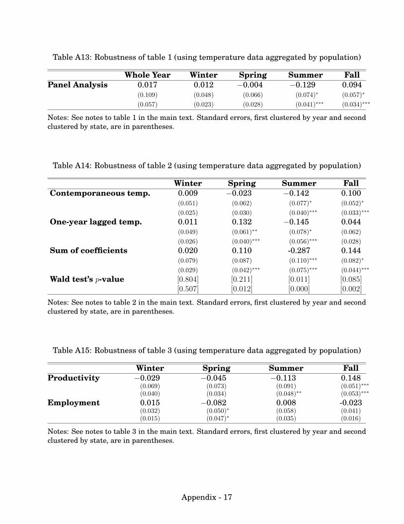
Table A13: Robustness of table 1 (using temperature data aggregated by population)

Whole Year Winter Spring Summer FallPanel Analysis 0.017 0.012 −0.004 −0.129 0.094

(0.109) (0.048) (0.066) (0.074)∗ (0.057)∗

(0.057) (0.023) (0.028) (0.041)∗∗∗ (0.034)∗∗∗

Notes: See notes to table 1 in the main text. Standard errors, first clustered by year and secondclustered by state, are in parentheses.

Table A14: Robustness of table 2 (using temperature data aggregated by population)

Winter Spring Summer FallContemporaneous temp. 0.009 −0.023 −0.142 0.100

(0.051) (0.062) (0.077)∗ (0.052)∗

(0.025) (0.030) (0.040)∗∗∗ (0.033)∗∗∗

One-year lagged temp. 0.011 0.132 −0.145 0.044(0.049) (0.061)∗∗ (0.078)∗ (0.062)

(0.026) (0.040)∗∗∗ (0.056)∗∗∗ (0.028)

Sum of coefficients 0.020 0.110 -0.287 0.144(0.079) (0.087) (0.110)∗∗∗ (0.082)∗

(0.029) (0.042)∗∗∗ (0.075)∗∗∗ (0.044)∗∗∗

Wald test’s p-value [0.804] [0.211] [0.011] [0.085][0.507] [0.012] [0.000] [0.002]

Notes: See notes to table 2 in the main text. Standard errors, first clustered by year and secondclustered by state, are in parentheses.

Table A15: Robustness of table 3 (using temperature data aggregated by population)

Winter Spring Summer FallProductivity −0.029 −0.045 −0.113 0.148

(0.069) (0.073) (0.091) (0.051)∗∗∗

(0.040) (0.034) (0.048)∗∗ (0.053)∗∗∗

Employment 0.015 −0.082 0.008 -0.023(0.032) (0.050)∗ (0.058) (0.041)(0.015) (0.047)∗ (0.035) (0.016)

Notes: See notes to table 3 in the main text. Standard errors, first clustered by year and secondclustered by state, are in parentheses.

Appendix - 17

Table A16: Robustness of table 4A (using temperature data aggregated by population)Pre-1997 Post-1997 Avg. GDP share (%)

Gross State Product −0.164 −0.187 100(0.104) (0.205)(0.054)∗∗∗ (0.072)∗∗∗

Services† 0.016 −0.122 25.7(0.072) (0.087)(0.049) (0.070)∗

Finance, insurance,real estate −0.249 -0.418 20.5(0.221) (0.373)(0.193) (0.144)∗∗∗

Manufacturing −0.019 0.333 12.9(0.217) (0.606)(0.098) (0.451)

Government −0.047 −0.038 12.2(0.077) (0.158)(0.051) (0.081)

Retail −0.041 −0.181 6.6(0.071) (0.185)(0.056) (0.090)∗∗

Wholesale −0.090 −0.217 5.9(0.105) (0.175)(0.062) (0.154)

Communication/Information† −0.182 −0.269 4.5(0.102)∗ (0.673)(0.080)∗∗ (0.355)

Construction −0.159 −0.390 4.4(0.234) (0.424)(0.185) (0.190)∗∗

Transportation 0.168 0.249 3.0(0.131) (0.195)(0.191) (0.119)∗∗

Utilities 0.357 0.600 1.8(0.229) (0.366)∗

(0.174)∗∗ (0.206)∗∗∗

Mining 0.048 0.596 1.4(0.543) (1.400)(0.522) (0.442)

Agriculture, forestry, fishing −2.500 −2.118 1.1(0.941)∗∗∗ (0.981)∗∗

(0.390)∗∗∗ (0.478)∗∗∗

Notes: See notes to table 4A in the main text. Standard errors, first clustered by year and secondclustered by state, are in parentheses.

Appendix - 18

Table A17: Robustness of table 4B (using temperature data aggregated by population)Post-1997 Ave GDP share (%)

ServicesProfessional and business services −0.083 11.6

(0.145)(0.085)

Educational services, health care, −0.011 7.7social assistance (0.045)

(0.064)

Other services, except government −0.136 2.6(0.122)(0.092)

Food services and drinking places −0.284 2.0(0.146)∗

(0.162)∗

Arts, entertainment, and recreation 0.354 1.0(0.268)(0.168)∗∗

Accommodation 0.091 0.9(0.246)(0.330)

Finance, insurance, real estateReal estate −0.407 11.4

(0.387)(0.113)∗∗∗

Federal Reserve banks, credit −0.184 3.6intermediation, and related services (0.415)

(0.280)

Insurance, carriers and related activities −1.419 2.6(0.612)∗∗

(0.539)∗∗∗

Securities, commodity contracts, −0.207 1.3and investments (0.512)

(0.297)

Rental and leasing services, lessors 0.008 1.3of intangible assets (0.272)

(0.271)

Funds, trusts, and other financial vehicles 1.243 0.2(1.201)(0.897)

Notes: See notes to table 4B in the main text. Standard errors, first clustered by year and secondclustered by state, are in parentheses.

Appendix - 19

Table A18: Robustness of table 5 (using temperature data aggregated by population)

Winter Spring Summer FallNorth 0.345 0.071 0.219 −0.355

(0.219) (0.285) (0.271) (0.266)(0.261) (0.191) (0.240) (0.144)∗∗

South −0.056 0.058 −0.263 0.515(0.153) (0.144) (0.161) (0.194)∗∗∗

(0.080) (0.082) (0.069)∗∗∗ (0.089)∗∗∗

Midwest 0.001 −0.174 0.093 −0.089(0.092) (0.156) (0.185) (0.139)(0.071) (0.118) (0.090) (0.082)

West 0.052 −0.145 0.102 −0.030(0.094) (0.143) (0.138) (0.151)(0.050) (0.067)∗∗ (0.144) (0.147)

Notes: See notes to table 5 in the main text. Standard errors, first clustered by year and secondclustered by state, are in parentheses.

Appendix - 20

A.6.3 Including one-year lagged temperatures

In this section, we show that our results are robust to including the one-year lag of

temperature in all specifications. We re-estimate our results in tables 3-5 including the

one-year lag of seasonal temperature variables. The results are reported in tables A19-

A23.

Table A19: Robustness of table 3 (including one-year lag of temperature)

Winter Spring Summer FallProductivity contemporaneous temp. −0.050 −0.040 −0.167 0.163

(0.066) (0.064) (0.090)∗ (0.054)∗∗∗

(0.035) (0.040) (0.055)∗∗∗ (0.076)∗∗

Productivity one-year lag −0.019 −0.023 −0.083 0.062(0.067) (0.065) (0.119) (0.071)(0.055) (0.026) (0.058) (0.119)

Sum of coefficients −0.069 −0.063 −0.250 0.225(0.114) (0.099) (0.141)∗ (0.112)∗∗

(0.067) (0.046) (0.068)∗∗∗ (0.182)

Wald test’s p-value [0.553] [0.531] [0.092] [0.058][0.309] [0.176] [0.001] [0.223]

Employment contemporaneous temp. 0.016 −0.083 0.002 −0.018(0.026) (0.040)∗∗ (0.064) (0.047)(0.016) (0.050)∗ (0.039) (0.028)

Employment one-year lag temp. 0.074 0.027 −0.136 −0.007(0.035)∗∗ (0.042) (0.052)∗∗∗ (0.048)(0.019)∗∗∗ (0.024) (0.050)∗∗∗ (0.022)

Sum of coefficients 0.090 −0.056 −0.134 −0.025(0.044)∗∗ (0.054) (0.098) (0.082)(0.031)∗∗∗ (0.034) (0.065)∗∗ (0.035)

Wald test’s p-value [0.053] [0.317] [0.187] [0.762][0.005] [0.108] [0.045] [0.474]

Notes: See notes to table 3 in the main text. Standard errors, first clustered by year and secondclustered by state, are in parentheses.

Appendix - 21

Table A20: Robustness of table 4A column 1 (including one-year lag of temperature)Contemp. One-year lag Sum of Wald test’s

temp. temp. coeff. p-valueGross state product −0.186 −0.116 −0.301

(0.095)∗ (0.113) (0.158)∗ [0.065](0.060)∗∗∗ (0.098) (0.123)∗∗ [0.018]

Services† 0.022 −0.187 −0.164(0.067) (0.061)∗∗∗ (0.092)∗ [0.084](0.049) (0.049)∗∗∗ (0.079)∗∗ [0.042]

Finance, insurance, real estate −0.205 −0.207 −0.412(0.243) (0.177) (0.331) [0.222](0.235) (0.143) (0.219)∗ [0.066]

Manufacturing −0.052 −0.221 −0.274(0.218) (0.192) (0.254) [0.289](0.104) (0.171) (0.153)∗ [0.079]

Government −0.068 0.019 −0.049(0.071) (0.062) (0.095) [0.608](0.063) (0.070) (0.107) [0.647]

Retail −0.050 −0.075 −0.125(0.075) (0.081) (0.102) [0.227](0.060) (0.059) (0.079) [0.119]

Wholesale −0.153 −0.161 −0.314(0.104) (0.107) (0.166)∗ [0.068](0.062)∗∗ (0.087)∗ (0.104)∗∗∗ [0.004]

Communication/Information† −0.238 0.073 −0.164(0.088)∗∗∗ (0.101) (0.148) [0.275](0.091)∗∗∗ (0.095) (0.122) [0.185]

Construction −0.216 −0.471 −0.688(0.238) (0.256)∗ (0.383)∗ [0.082](0.184) (0.230)∗∗ (0.360)∗ [0.062]

Transportation 0.151 −0.037 0.114(0.124) (0.149) (0.213) [0.595](0.195) (0.097) (0.254) [0.654]

Utilities 0.337 0.028 0.364(0.249) (0.184) (0.283) [0.207](0.202)∗ (0.160) (0.258) [0.164]

Mining −0.162 0.138 −0.024(0.538) (0.706) (0.817) [0.977](0.539) (0.730) (1.189) [0.984]

Agriculture, forestry, fishing −2.556 1.338 −1.218(0.966)∗∗∗ (0.700)∗ (1.292) [0.353](0.444)∗∗∗ (0.316)∗∗∗ (0.369)∗∗∗ [0.002]

Notes: See notes to table 4A in the main text. Standard errors, first clustered by year and secondclustered by state, are in parentheses.

Appendix - 22

Table A21: Robustness of table 4A column 2 (including one-year lag of temperature)Contemp. One-year lag Sum of Wald test’s

temp. temp. coeff. p-valueGross state product −0.269 −0.223 −0.492

(0.183) (0.151) (0.212)∗∗ [0.039](0.069)∗∗∗ (0.090)∗∗ (0.121)∗∗∗ [0.000]

Services† −0.230 −0.242 −0.472(0.068)∗∗∗ (0.132)∗ (0.162)∗∗∗ [0.013](0.080)∗∗∗ (0.127)∗ (0.176)∗∗∗ [0.010]

Finance, insurance, real estate −0.454 −0.184 −0.638(0.385) (0.278) (0.561) [0.278](0.155)∗∗∗ (0.128) (0.205)∗∗∗ [0.003]

Manufacturing 0.014 −0.576 −0.562(0.622) (0.515) (0.821) [0.507](0.410) (0.416) (0.492) [0.259]

Government −0.071 −0.267 −0.338(0.159) (0.148)∗ (0.238) [0.180](0.085) (0.141)∗ (0.163)∗∗ [0.043]

Retail −0.251 −0.093 −0.343(0.200) (0.202) (0.333) [0.323](0.083)∗∗∗ (0.070) (0.103)∗∗∗ [0.002]

Wholesale −0.294 −0.116 −0.410(0.173)∗ (0.124) (0.231)∗ [0.101](0.160)∗ (0.081) (0.157)∗∗∗ [0.012]

Communication/Information† −0.298 −0.045 −0.343(0.739) (0.291) (0.870) [0.701](0.388) (0.323) (0.321) [0.290]

Construction −0.410 −0.390 −0.800(0.442) (0.338) (0.612) [0.215](0.189)∗∗ (0.186)∗∗ (0.267)∗∗∗ [0.004]

Transportation 0.201 0.167 0.368(0.216) (0.256) (0.367) [0.337](0.140) (0.145) (0.254) [0.153]

Utilities 0.605 −0.209 0.396(0.341)∗ (0.509) (0.488) [0.433](0.252)∗∗ (0.387) (0.580) [0.498]

Mining 0.844 1.673 2.516(1.593) (1.361) (1.848) [0.198](0.356)∗∗ (0.718)∗∗ (0.645)∗∗∗ [0.000]

Agriculture, forestry, fishing −2.091 1.817 −0.274(0.999)∗∗ (1.106)∗ (1.764) [0.879](0.463)∗∗∗ (0.758)∗∗ (0.852) [0.749]

Notes: See notes to table 4A in the main text. Standard errors, first clustered by year and secondclustered by state, are in parentheses.

Appendix - 23

Table A22: Robustness of table 4B (including one-year lag of temperature)Contemp. One-year Sum of Wald test’s

temp. lag temp. coeff. p-valueServices

Professional and business services −0.258 −0.391 −0.649(0.103)∗∗ (0.223)∗ (0.234)∗∗∗ [0.017](0.113)∗∗ (0.225)∗ (0.307)∗∗ [0.039]

Educational services, −0.007 −0.022 −0.028health care, social assistance (0.048) (0.061) (0.085) [0.746]

(0.065) (0.047) (0.087) [0.745]Other services, except government −0.274 −0.257 −0.531

(0.147)∗ (0.178) (0.277)∗ [0.079](0.104)∗∗∗ (0.154)∗ (0.214)∗∗ [0.016]

Food services and drinking places −0.392 −0.063 −0.455(0.158)∗∗ (0.243) (0.321) [0.181](0.148)∗∗∗ (0.067) (0.180)∗∗ [0.015]

Arts, entertainment, and recreation 0.371 −0.439 −0.068(0.258) (0.247)∗ (0.419) [0.873](0.202)∗ (0.160)∗∗∗ (0.281) [0.809]

Accommodation 0.015 −0.182 −0.167(0.275) (0.240) (0.460) [0.723](0.365) (0.177) (0.489) [0.734]

Finance, insurance, real estateReal estate −0.460 −0.268 −0.728

(0.402) (0.234) (0.572) [0.227](0.121)∗∗∗ (0.112)∗∗ (0.181)∗∗∗ [0.000]

Federal Reserve banks, credit −0.271 −0.185 −0.456intermediation, and related services (0.455) (0.246) (0.443) [0.324]

(0.364) (0.370) (0.611) [0.459]Insurance, carriers −1.310 -0.124 −1.435and related activities (0.624)∗∗ (0.595) (0.837)∗ [0.112]

(0.539)∗∗ (0.513) (0.684)∗∗ [0.041]Securities, commodity contracts, −0.310 −0.167 −0.477and investments (0.574) (0.611) (1.012) [0.646]

(0.329) (0.412) (0.526) [0.368]Rental and leasing services, −0.035 −0.081 −0.116lessors of intangible assets (0.250) (0.419) (0.558) [0.839]

(0.292) (0.334) (0.487) [0.813]Funds, trusts, and 0.984 −0.442 0.542other financial vehicles (1.067) (1.156) (1.175) [0.653]

(1.143) (1.591) (2.344) [0.818]

Notes: See notes to table 4B in the main text. Standard errors, first clustered by year and secondclustered by state, are in parentheses.

Appendix - 24

Table A23: Robustness of table 5 (including one-year lag of temperature)

Winter Spring Summer FallNorth contemp. 0.276 0.063 0.115 −0.224

(0.165)∗ (0.301) (0.268) (0.236)(0.225) (0.170) (0.220) (0.163)

North one-year lag 0.263 0.300 −0.022 0.114(0.205) (0.196) (0.306) (0.225)(0.162) (0.197) (0.224) (0.242)

Sum of coefficients 0.539 0.363 0.093 −0.111(0.262)∗∗ (0.339) (0.333) (0.257)(0.335) (0.244) (0.438) (0.319)

Wald test’s p-value [0.045] [0.290] [0.781] [0.668][0.147] [0.175] [0.837] [0.738]

South contemp. −0.102 0.049 −0.325 0.549(0.167) (0.138) (0.173)∗ (0.179)∗∗∗

(0.092) (0.051) (0.087)∗∗∗ (0.054)∗∗∗

South one-year lag 0.009 0.152 −0.390 0.326(0.120) (0.182) (0.207)∗ (0.187)∗

(0.082) (0.086)∗ (0.141)∗∗∗ (0.111)∗∗∗

Sum of coefficients −0.092 0.201 −0.715 0.876(0.195) (0.211) (0.244)∗∗∗ (0.285)∗∗∗

(0.069) (0.082)∗∗ (0.182)∗∗∗ (0.147)∗∗∗

Wald test’s p-value [0.638] [0.343] [0.005] [0.003][0.197] [0.026] [0.001] [0.000]

Midwest contemp. −0.017 −0.223 −0.003 −0.162(0.084) (0.140) (0.159) (0.115)(0.054) (0.098)∗∗ (0.069) (0.078) ∗∗

Midwest one-year lag −0.126 0.243 −0.154 0.176(0.090) (0.142) ∗ (0.161) (0.115)(0.060) ∗∗ (0.105) ∗∗ (0.131) (0.076) ∗∗

Sum of coefficients −0.143 0.020 −0.157 0.015(0.119) (0.20)3 (0.255) (0.157)(0.091) (0.113) (0.116) (0.083)

Wald test’s p-value [0.235] [0.921] [0.540] [0.927][0.143] [0.861] [0.204] [0.864]

West contemp. 0.018 −0.121 0.068 −0.014(0.096) (0.149) (0.147) (0.168)(0.069) (0.069)∗ (0.149) (0.165)

West one-year lag 0.057 0.047 −0.152 -0.069(0.124) (0.162) (0.149) (0.150)(0.072) (0.169) (0.116) (0.082)

Sum of coefficients 0.075 −0.075 −0.083 −0.083(0.165) (0.253) (0.221) (0.249)(0.094) (0.213) (0.212) (0.115)

Wald test’s p-value [0.650] [0.769] [0.708] [0.739][0.440] [0.732] [0.702] [0.482]

Notes: See notes to table 5 in the main text. Standard errors, first clustered by year and secondclustered by state, are in parentheses.

Appendix - 25

A.6.4 Arellano-Bond estimator

In this section, we show that our results in tables 1-5 are robust to using GMM esti-

mators developed by (Arellano and Bond, 1991) that produce consistent estimates of a

dynamic panel for finite T . We use first differences with respect to time. Because T

is fairly large, using all possible instruments could lead to a bias of “too many instru-

ments” (Newey and Windmeijer (2009)), so we restrict the number of intruments and

use one step GMM estimators with a naive weighting matrix. These estimators remain

consistent when T (the number of time periods) and N (the number of states) and the

number of instruments is large (Alvarez and Arellano (2003)). We use lags 2-10 as in-

struments, use small sample adjustments, and estimate robust standard errors. The

results are reported in tables A24-A29.

Table A24: Robustness of table 1 (using Arellano-Bond)

Whole Year Winter Spring Summer FallPanel Analysis −0.026 −0.002 −0.049 −0.134 0.115

(0.082) (0.032) (0.034) (0.042)∗∗∗ (0.056)∗∗

Notes: See notes to table 1 in the main text. Robust standard errors are in parentheses.

Table A25: Robustness of table 2 (using Arellano-Bond)

Winter Spring Summer FallContemporaneous temp. −0.020 −0.059 −0.191 0.143

(0.034) (0.030)∗ (0.043)∗∗∗ (0.054)∗∗∗

One-year lagged temp. 0.012 0.083 −0.137 0.126(0.027) (0.048)∗ (0.055)∗∗ (0.040)∗∗∗

Sum of coefficients −0.008 0.024 −0.328 0.270(0.043) (0.052) (0.075)∗∗∗ ((0.083)∗∗∗

Wald test’s p-value [0.860] [0.651] [0.000] [0.002]

Notes: See notes to table 2 in the main text. Robust standard errors are in parentheses.

Appendix - 26

Table A26: Robustness of table 3 (using Arellano-Bond)

Winter Spring Summer FallProductivity −0.011 0.002 −0.152 0.142

(0.050) (0.052) (0.065)∗∗ (0.059)∗∗

Employment −0.004 −0.068 0.048 −0.012(0.016) (0.032)∗∗ (0.036) (0.021)

Notes: See notes to table 3 in the main text. Robust standard errors are in parentheses.

Table A27: Robustness of table 4A (using Arellano-Bond)Pre-1997 Post-1997 Avg. GDP share (%)

Gross state product −0.164 −0.236 100(0.061)∗∗∗ (0.067)∗∗∗

Services† 0.110 −0.165 25.7(0.046)∗∗ (0.076)∗∗

Finance, insurance, real estate −0.137 −0.505 20.5(0.227) (0.179)∗∗∗

Manufacturing −0.052 0.344 12.9(0.148) (0.512)

Government −0.101 −0.011 12.2(0.057)∗ (0.104)

Retail −0.011 −0.122 6.6(0.075) (0.108)

Wholesale −0.136 −0.267 5.9(0.081)∗ (0.165)

Communication/Information† −0.223 −0.066 4.5(0.135)* (0.423)

Construction −0.038 −0.218 4.4(0.148) (0.226)

Transportation 0.243 0.131 3.0(0.287) (0.114)

Utilities 0.454 0.129 1.8(0.202)∗∗ (0.340)

Mining −0.110 0.272 1.4(0.526) (0.324)

Agriculture, forestry, fishing −3.054 −2.456 1.1(0.486)∗∗∗ (0.690)∗∗∗

Notes: See notes to table 4A in the main text. Robust standard errors are in parentheses.

Appendix - 27

Table A28: Robustness of table 4B (using Arellano-Bond)Post-1997 Ave GDP share (%)

ServicesProfessional and business services −0.102 11.6

(0.095)

Educational services, health care, −0.044 7.7social assistance (0.067)

Other services, except government −0.238 2.6(0.108)∗∗

Food services and drinking places −0.339 2.0(0.152)∗∗

Arts, entertainment, and recreation 0.513 1.0(0.194)∗∗∗

Accommodation 0.219 0.9(0.273)

Finance, insurance, real estateReal estate −0.640 11.4

(0.134)∗∗∗

Federal Reserve banks, credit −0.181 3.6intermediation, and related services (0.304)

Insurance, carriers and related activities −1.637 2.6(0.673)∗∗

Securities, commodity contracts, 0.309 1.3and investments (0.376)

Rental and leasing services, lessors 0.149 1.3of intangible assets (0.320)

Funds, trusts, and other financial vehicles 1.176 0.2(0.847)

Notes: See notes to table 4B in the main text. Robust standard errors are in parentheses.

Table A29: Robustness of table 5 (using Arellano-Bond)

Winter Spring Summer FallNorth 0.322 0.079 0.205 −0.236

(0.248) (0.194) (0.225) (0.168)

South −0.115 0.148 −0.257 0.672(0.096) (0.136) (0.096)∗∗∗ (0.069)∗∗∗

Midwest −0.010 −0.156 0.028 −0.108(0.059) (0.103) (0.076) (0.084)

West −0.029 −0.087 0.053 0.002(0.069) (0.070) (0.178) (0.174)

Notes: See notes to table 5 in the main text. Robust standard errors are in parentheses.

Appendix - 28