![A Selected Survey of Umbral Calculus · 2000-04-12 · methods. However, only the subclass of polynomials of binomial type are treated in [289]. The extension to Sheffer polynomials](https://static.fdocuments.us/doc/165x107/5f039b347e708231d409e1db/a-selected-survey-of-umbral-calculus-2000-04-12-methods-however-only-the-subclass.jpg)
Telephone Numbers and the Umbral Calculus - LSU … · · 2018-05-18Telephone Numbers and the...
115
Telephone Numbers and the Umbral Calculus April Chow 1 Iris Gray 1 Lawrence Mouillé 2 James Pickett 3 1 Louisiana State University Baton Rouge, LA 2 University of Louisiana at Lafayette Lafayette, LA 3 University of South Alabama Mobile, AL SMILE @ LSU 2013, July 12, 2013
-
Upload
nguyenthuan -
Category
Documents
-
view
220 -
download
0
Transcript of Telephone Numbers and the Umbral Calculus - LSU … · · 2018-05-18Telephone Numbers and the...

Telephone Numbers and the Umbral Calculus
April Chow1 Iris Gray1
Lawrence Mouillé2 James Pickett3
1Louisiana State UniversityBaton Rouge, LA
2University of Louisiana at LafayetteLafayette, LA
3University of South AlabamaMobile, AL
SMILE @ LSU 2013, July 12, 2013

t4 Possible Conversations

t4 Possible Conversations

t6 Possible Conversations
There are 76 ways to have these conversations.

t6 Possible Conversations
There are 76 ways to have these conversations.

Calculation of t0 to t10
# of users Ways of Calling0 11 12 23 44 105 266 767 2328 7649 2620
10 9496

Calculation of t0 to t10
# of users Ways of Calling0 11 12 23 44 105 266 767 2328 7649 2620
10 9496

Recursion Relation of tn
The telephone numbers satisfy the following recursion:
tn = tn−1 + (n − 1)tn−2,
where t0 and t1 are both equal to 1.
Proof.
Either user 1 is making a call or user 1 is not making a call.• If user 1 is not making a call, there are tn−1 ways that the
network of n − 1 remaining users can be configured.Hence, the tn−1 term.
• If user 1 is making a call, we may choose who he is callingn − 1 different ways. In each n − 1 case, there are n − 2users remaining. Hence, the (n − 1)tn−2 term.

Recursion Relation of tn
The telephone numbers satisfy the following recursion:
tn = tn−1 + (n − 1)tn−2,
where t0 and t1 are both equal to 1.
Proof.
Either user 1 is making a call or user 1 is not making a call.
• If user 1 is not making a call, there are tn−1 ways that thenetwork of n − 1 remaining users can be configured.Hence, the tn−1 term.
• If user 1 is making a call, we may choose who he is callingn − 1 different ways. In each n − 1 case, there are n − 2users remaining. Hence, the (n − 1)tn−2 term.

Recursion Relation of tn
The telephone numbers satisfy the following recursion:
tn = tn−1 + (n − 1)tn−2,
where t0 and t1 are both equal to 1.
Proof.
Either user 1 is making a call or user 1 is not making a call.• If user 1 is not making a call, there are tn−1 ways that the
network of n − 1 remaining users can be configured.Hence, the tn−1 term.
• If user 1 is making a call, we may choose who he is callingn − 1 different ways. In each n − 1 case, there are n − 2users remaining. Hence, the (n − 1)tn−2 term.

Recursion Relation of tn
The telephone numbers satisfy the following recursion:
tn = tn−1 + (n − 1)tn−2,
where t0 and t1 are both equal to 1.
Proof.
Either user 1 is making a call or user 1 is not making a call.• If user 1 is not making a call, there are tn−1 ways that the
network of n − 1 remaining users can be configured.Hence, the tn−1 term.
• If user 1 is making a call, we may choose who he is callingn − 1 different ways. In each n − 1 case, there are n − 2users remaining. Hence, the (n − 1)tn−2 term.

The Closed Formula of tn
Theorem
tn =
b n2 c∑
k=0
n!2kk !(n − 2k)!
Exponential Generating Functions
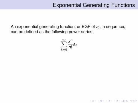
An exponential generating function, or EGF of an, a sequence,can be defined as the following power series:
∞∑k=0
xn
n!an
TheoremThe EGF of tn is
T (x) =∞∑
k=0
tnn!
xn = ex+ x22 .
Exponential Generating Functions
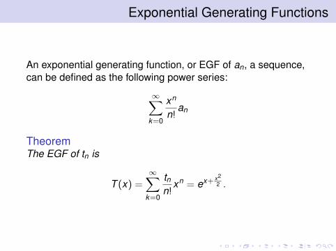
An exponential generating function, or EGF of an, a sequence,can be defined as the following power series:
∞∑k=0
xn
n!an
TheoremThe EGF of tn is
T (x) =∞∑
k=0
tnn!
xn = ex+ x22 .

The EGF of tn
Proof.Now, recall that tn+1 = tn + ntn−1. In terms of the summation:
∞∑n=1
tn+1
n!xn =
∞∑n=1
tnn!
xn +∞∑
n=1
n tn−1
n!xn
•∞∑
n=1
tn+1
n!xn = T ′(x)− 1.
•∞∑
n=1
tnn!
xn = T (x)− 1.
•∞∑
n=1
n tn−1
n!xn = xT ′(x).

The EGF of tn
Proof.Now, recall that tn+1 = tn + ntn−1. In terms of the summation:
∞∑n=1
tn+1
n!xn =
∞∑n=1
tnn!
xn +∞∑
n=1
n tn−1
n!xn
•∞∑
n=1
tn+1
n!xn = T ′(x)− 1.
•∞∑
n=1
tnn!
xn = T (x)− 1.
•∞∑
n=1
n tn−1
n!xn = xT ′(x).

The EGF of tn
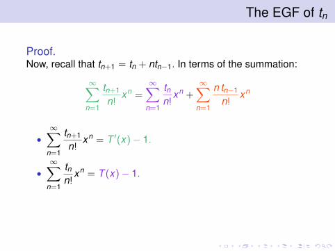
Proof.Now, recall that tn+1 = tn + ntn−1. In terms of the summation:
∞∑n=1
tn+1
n!xn =
∞∑n=1
tnn!
xn +∞∑
n=1
n tn−1
n!xn
•∞∑
n=1
tn+1
n!xn = T ′(x)− 1.
•∞∑
n=1
tnn!
xn = T (x)− 1.
•∞∑
n=1
n tn−1
n!xn = xT ′(x).
The EGF of tn
Proof.Now, recall that tn+1 = tn + ntn−1. In terms of the summation:
∞∑n=1
tn+1
n!xn =
∞∑n=1
tnn!
xn +∞∑
n=1
n tn−1
n!xn
•∞∑
n=1
tn+1
n!xn = T ′(x)− 1.
•∞∑
n=1
tnn!
xn = T (x)− 1.
•∞∑
n=1
n tn−1
n!xn = xT ′(x).

The EGF of tn
Proof.Now, recall that tn+1 = tn + ntn−1. In terms of the summation:
∞∑n=1
tn+1
n!xn =
∞∑n=1
tnn!
xn +∞∑
n=1
n tn−1
n!xn
•∞∑
n=1
tn+1
n!xn = T ′(x)− 1.
•∞∑
n=1
tnn!
xn = T (x)− 1.
•∞∑
n=1
n tn−1
n!xn = xT ′(x).
The EGF of tn (cont.)
Proof (Cont.)Solving for T (x) :
T ′(x)− 1 = T (x)− 1 + xT ′(x).
Now,T ′(x) = (1 + x)T (x),
where T (0) = 1
=⇒ T (x) = ex+ x22

The EGF of tn (cont.)
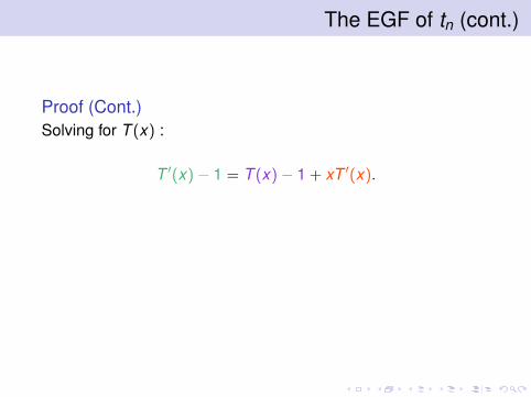
Proof (Cont.)Solving for T (x) :
T ′(x)− 1 = T (x)− 1 + xT ′(x).
Now,T ′(x) = (1 + x)T (x),
where T (0) = 1
=⇒ T (x) = ex+ x22

Hermite Polynomials
The set of Hermite polynomials is a polynomial sequence.
Applications of Hermite Polynomials:
• Probability;• Numerical Analysis;• Combinatorics;• Physics.

Hermite Polynomials
The set of Hermite polynomials is a polynomial sequence.
Applications of Hermite Polynomials:
• Probability;
• Numerical Analysis;• Combinatorics;• Physics.

Hermite Polynomials
The set of Hermite polynomials is a polynomial sequence.
Applications of Hermite Polynomials:
• Probability;• Numerical Analysis;
• Combinatorics;• Physics.

Hermite Polynomials
The set of Hermite polynomials is a polynomial sequence.
Applications of Hermite Polynomials:
• Probability;• Numerical Analysis;• Combinatorics;
• Physics.

Hermite Polynomials
The set of Hermite polynomials is a polynomial sequence.
Applications of Hermite Polynomials:
• Probability;• Numerical Analysis;• Combinatorics;• Physics.

Hermite Polynomials
Definition
Hn(u) = n!bn/2c∑k=0
(−1)k
k ! (n − 2k)!(2u)n−2k

H0(u) to H10(u)
n Hn(u)0 11 2u2 2(−1 + 2u2)
3 6(−2u + 4u3
3 )
4 24(12 − 2u2 + 2u4
3 )
5 120(u − 4u3
3 + 4u5
15 )
6 720(−16 + u2 − 2u4
3 + 4u6
45 )
7 5040(−u3 + 2u3
3 −4u5
15 + 8u7
315)
8 40320( 124 −
u2
3 + u4
3 −4u6
45 + 2u8
315)
9 362880( u12 −
2u3
9 + 2u5
15 −8u7
315 + 4u9
2835)
10 3628800(− 1120 + u2
12 −u4
9 + 2u6
45 −2u8
315 + 4u10
14175)

Relating Hn and tn
Observe (i√2
)0
H0
(−i√
2
)= 1 = t0
(i√2
)1
H1
(−i√
2
)= 1 = t1
(i√2
)2
H2
(−i√
2
)= 2 = t2
(i√2
)3
H3
(−i√
2
)= 4 = t3

Relating Hn and tn
Observe (i√2
)0
H0
(−i√
2
)= 1 = t0
(i√2
)1
H1
(−i√
2
)= 1 = t1
(i√2
)2
H2
(−i√
2
)= 2 = t2
(i√2
)3
H3
(−i√
2
)= 4 = t3

Relating Hn and tn
Observe (i√2
)0
H0
(−i√
2
)= 1 = t0
(i√2
)1
H1
(−i√
2
)= 1 = t1
(i√2
)2
H2
(−i√
2
)= 2 = t2
(i√2
)3
H3
(−i√
2
)= 4 = t3

Relating Hn and tn
Observe (i√2
)0
H0
(−i√
2
)= 1 = t0
(i√2
)1
H1
(−i√
2
)= 1 = t1
(i√2
)2
H2
(−i√
2
)= 2 = t2
(i√2
)3
H3
(−i√
2
)= 4 = t3
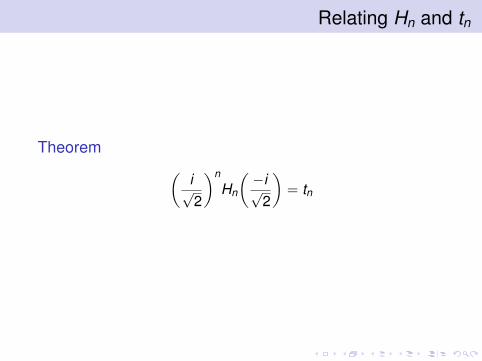
Relating Hn and tn
Theorem (i√2
)n
Hn
(−i√
2
)= tn
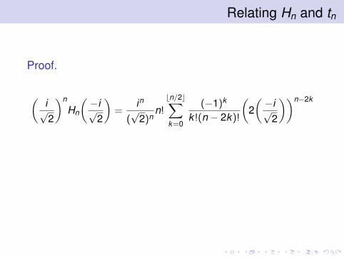
Relating Hn and tn
Proof.
(i√2
)n
Hn
(−i√
2
)=
in
(√
2)nn!bn/2c∑k=0
(−1)k
k !(n − 2k)!
(2(−i√
2
))n−2k
=
bn/2c∑k=0
n!2kk !(n − 2k)!
= tn

Relating Hn and tn
Proof.
(i√2
)n
Hn
(−i√
2
)=
in
(√
2)nn!bn/2c∑k=0
(−1)k
k !(n − 2k)!
(2(−i√
2
))n−2k
=
bn/2c∑k=0
n!2kk !(n − 2k)!
= tn

Relating Hn and tn
Proof.
(i√2
)n
Hn
(−i√
2
)=
in
(√
2)nn!bn/2c∑k=0
(−1)k
k !(n − 2k)!
(2(−i√
2
))n−2k
=
bn/2c∑k=0
n!2kk !(n − 2k)!
= tn

The Umbral Method
Suppose an is given and we define another sequence
bn =n∑
k=0
(nk
)ak
We wish to solve for an in terms of bk , and will use the umbrae.
Bn =n∑
k=0
(nk
)Ak

The Umbral Method
Suppose an is given and we define another sequence
bn =n∑
k=0
(nk
)ak
We wish to solve for an in terms of bk , and will use the umbrae.
Bn =n∑
k=0
(nk
)Ak

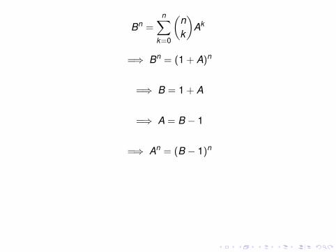
Bn =n∑
k=0
(nk
)Ak
=⇒ Bn = (1 + A)n
=⇒ B = 1 + A
=⇒ A = B − 1
=⇒ An = (B − 1)n
=⇒ An =n∑
k=0
(nk
)Bk (−1)n−k
=⇒ an =n∑
k=0
(nk
)bk (−1)n−k

Bn =n∑
k=0
(nk
)Ak
=⇒ Bn = (1 + A)n
=⇒ B = 1 + A
=⇒ A = B − 1
=⇒ An = (B − 1)n
=⇒ An =n∑
k=0
(nk
)Bk (−1)n−k
=⇒ an =n∑
k=0
(nk
)bk (−1)n−k

Bn =n∑
k=0
(nk
)Ak
=⇒ Bn = (1 + A)n
=⇒ B = 1 + A
=⇒ A = B − 1
=⇒ An = (B − 1)n
=⇒ An =n∑
k=0
(nk
)Bk (−1)n−k
=⇒ an =n∑
k=0
(nk
)bk (−1)n−k

Bn =n∑
k=0
(nk
)Ak
=⇒ Bn = (1 + A)n
=⇒ B = 1 + A
=⇒ A = B − 1
=⇒ An = (B − 1)n
=⇒ An =n∑
k=0
(nk
)Bk (−1)n−k
=⇒ an =n∑
k=0
(nk
)bk (−1)n−k
Bn =n∑
k=0
(nk
)Ak
=⇒ Bn = (1 + A)n
=⇒ B = 1 + A
=⇒ A = B − 1
=⇒ An = (B − 1)n
=⇒ An =n∑
k=0
(nk
)Bk (−1)n−k
=⇒ an =n∑
k=0
(nk
)bk (−1)n−k

Bn =n∑
k=0
(nk
)Ak
=⇒ Bn = (1 + A)n
=⇒ B = 1 + A
=⇒ A = B − 1
=⇒ An = (B − 1)n
=⇒ An =n∑
k=0
(nk
)Bk (−1)n−k
=⇒ an =n∑
k=0
(nk
)bk (−1)n−k

Bn =n∑
k=0
(nk
)Ak
=⇒ Bn = (1 + A)n
=⇒ B = 1 + A
=⇒ A = B − 1
=⇒ An = (B − 1)n
=⇒ An =n∑
k=0
(nk
)Bk (−1)n−k
=⇒ an =n∑
k=0
(nk
)bk (−1)n−k
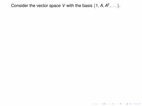
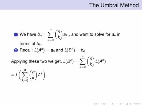
Consider the vector space V with the basis {1,A,A2, . . . }.
Vectors in V are polynomials of the form
p(A) =d∑
k=0
ckAk
Define the linear functional L : V → R such that L(An) = an.
Then,
L(p(A)) = L(d∑
k=0
ckAk ) =d∑
k=0
ckL(Ak )
• A is the umbra of an.• Many formulas are easier to derive if we change an to An
for some variable A. After some algebraic manipulation ,we change An back to an.

Consider the vector space V with the basis {1,A,A2, . . . }.
Vectors in V are polynomials of the form
p(A) =d∑
k=0
ckAk
Define the linear functional L : V → R such that L(An) = an.
Then,
L(p(A)) = L(d∑
k=0
ckAk ) =d∑
k=0
ckL(Ak )
• A is the umbra of an.
• Many formulas are easier to derive if we change an to An
for some variable A. After some algebraic manipulation ,we change An back to an.

Consider the vector space V with the basis {1,A,A2, . . . }.
Vectors in V are polynomials of the form
p(A) =d∑
k=0
ckAk
Define the linear functional L : V → R such that L(An) = an.
Then,
L(p(A)) = L(d∑
k=0
ckAk ) =d∑
k=0
ckL(Ak )
• A is the umbra of an.• Many formulas are easier to derive if we change an to An
for some variable A. After some algebraic manipulation ,we change An back to an.

The Umbral Method
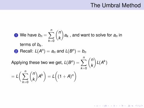
1 We have bn =n∑
k=0
(nk
)ak , and want to solve for an in
terms of bk .2 Recall: L(An) = an and L(Bn) = bn
Applying these two we get, L(Bn) =n∑
k=0
(nk
)L(Ak )
= L( n∑
k=0
(nk
)Ak)
= L((1 + A)n
)

The Umbral Method
1 We have bn =n∑
k=0
(nk
)ak , and want to solve for an in
terms of bk .2 Recall: L(An) = an and L(Bn) = bn
Applying these two we get, L(Bn) =n∑
k=0
(nk
)L(Ak )
= L( n∑
k=0
(nk
)Ak)
= L((1 + A)n
)
The Umbral Method
1 We have bn =n∑
k=0
(nk
)ak , and want to solve for an in
terms of bk .2 Recall: L(An) = an and L(Bn) = bn
Applying these two we get, L(Bn) =n∑
k=0
(nk
)L(Ak )
= L( n∑
k=0
(nk
)Ak)
= L((1 + A)n
)
The Umbral Method
1 We have bn =n∑
k=0
(nk
)ak , and want to solve for an in
terms of bk .2 Recall: L(An) = an and L(Bn) = bn
Applying these two we get, L(Bn) =n∑
k=0
(nk
)L(Ak )
= L( n∑
k=0
(nk
)Ak)
= L((1 + A)n
)

The Umbral Method
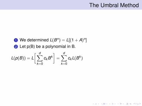
1 We determined L(Bn) = L[(1 + A)n]
2 Let p(B) be a polynomial in B.
L(p(B)) = L[ d∑
k=0
ckBk]=
d∑k=0
ckL(Bk ) =d∑
k=0
ckL[(1 + A)k ]
= L(p(1 + A))

The Umbral Method
1 We determined L(Bn) = L[(1 + A)n]
2 Let p(B) be a polynomial in B.
L(p(B)) = L[ d∑
k=0
ckBk]
=d∑
k=0
ckL(Bk ) =d∑
k=0
ckL[(1 + A)k ]
= L(p(1 + A))
The Umbral Method
1 We determined L(Bn) = L[(1 + A)n]
2 Let p(B) be a polynomial in B.
L(p(B)) = L[ d∑
k=0
ckBk]=
d∑k=0
ckL(Bk )
=d∑
k=0
ckL[(1 + A)k ]
= L(p(1 + A))

The Umbral Method
1 We determined L(Bn) = L[(1 + A)n]
2 Let p(B) be a polynomial in B.
L(p(B)) = L[ d∑
k=0
ckBk]=
d∑k=0
ckL(Bk ) =d∑
k=0
ckL[(1 + A)k ]
= L(p(1 + A))

The Umbral Method
1 We determined L(Bn) = L[(1 + A)n]
2 Let p(B) be a polynomial in B.
L(p(B)) = L[ d∑
k=0
ckBk]=
d∑k=0
ckL(Bk ) =d∑
k=0
ckL[(1 + A)k ]
= L(p(1 + A))
The Umbral Method
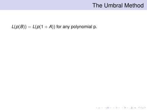
L(p(B)) = L(p(1 + A)) for any polynomial p.
p(B) = (B − 1)n
L(B − 1)n = L((1 + A− 1)n) = L(An)
L( n∑
k=0
(nk
)Bk (−1)n−k
)= L(An)
n∑k=0
(nk
)bk (−1)n−k = an

The Umbral Method
L(p(B)) = L(p(1 + A)) for any polynomial p.
p(B) = (B − 1)n
L(B − 1)n = L((1 + A− 1)n) = L(An)
L( n∑
k=0
(nk
)Bk (−1)n−k
)= L(An)
n∑k=0
(nk
)bk (−1)n−k = an

The Umbral Method
L(p(B)) = L(p(1 + A)) for any polynomial p.
p(B) = (B − 1)n
L(B − 1)n = L((1 + A− 1)n) = L(An)
L( n∑
k=0
(nk
)Bk (−1)n−k
)= L(An)
n∑k=0
(nk
)bk (−1)n−k = an

The Umbral Method
L(p(B)) = L(p(1 + A)) for any polynomial p.
p(B) = (B − 1)n
L(B − 1)n = L((1 + A− 1)n) = L(An)
L( n∑
k=0
(nk
)Bk (−1)n−k
)= L(An)
n∑k=0
(nk
)bk (−1)n−k = an

The Umbral Method
L(p(B)) = L(p(1 + A)) for any polynomial p.
p(B) = (B − 1)n
L(B − 1)n = L((1 + A− 1)n) = L(An)
L( n∑
k=0
(nk
)Bk (−1)n−k
)= L(An)
n∑k=0
(nk
)bk (−1)n−k = an

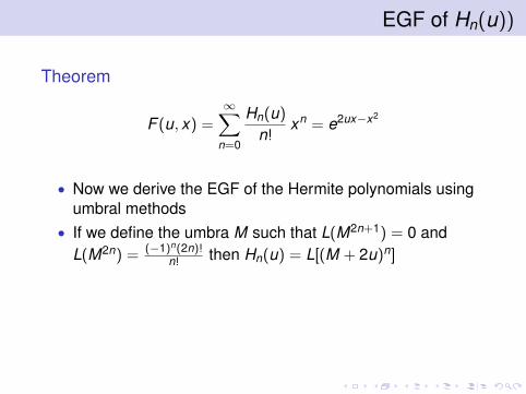
EGF of Hn(u))
Theorem
F (u, x) =∞∑
n=0
Hn(u)n!
xn = e2ux−x2
• Now we derive the EGF of the Hermite polynomials usingumbral methods
• If we define the umbra M such that L(M2n+1) = 0 andL(M2n) = (−1)n(2n)!
n! then Hn(u) = L[(M + 2u)n]
• Then we have,
∞∑n=0
Hn(u)n!
xn = L(e(M+2u)x) = e2uxL(eMx) = e2uxe−x2= e2ux−x2
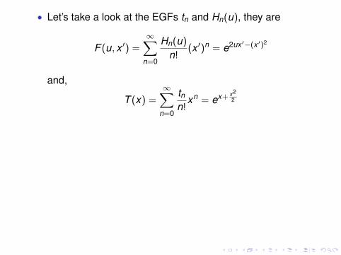
• Let’s take a look at the EGFs tn and Hn(u), they are
F (u, x ′) =∞∑
n=0
Hn(u)n!
(x ′)n = e2ux ′−(x ′)2
and,
T (x) =∞∑
n=0
tnn!
xn = ex+ x22
• Notice any similarities? Choosing u and x ′ for F (u, x ′)appropriately we can achieve equality. Those choiceswould be, u = −i√
2and x ′ = ix√
2
• Proof.
F(−i√
2,
ix√2
)= e2
(−i√
2
)(ix√
2
)−(
ix√2
)2
= ex+ 12 x2
= T (x)

Relating Hn and tn
• Writing the EGFs in their power series representations with
F(−i√
2, ix√
2
)= T (x) we have
•∞∑
n=0
Hn( −i√
2
)n!
( ix√2
)n=∞∑
n=0
tnn!
xn.
Hence, for all n
Hn( −i√
2
)n!
( ix√2
)n=
tnn!
xn.
Therefore, (i√2
)n
Hn
(−i√
2
)= tn.

Relating Hn and tn
• Writing the EGFs in their power series representations with
F(−i√
2, ix√
2
)= T (x) we have
•∞∑
n=0
Hn( −i√
2
)n!
( ix√2
)n=∞∑
n=0
tnn!
xn.
Hence, for all n
Hn( −i√
2
)n!
( ix√2
)n=
tnn!
xn.
Therefore, (i√2
)n
Hn
(−i√
2
)= tn.

Further Applications
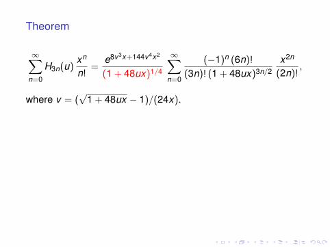
Theorem
∞∑n=0
H3n(u)xn
n!=
e8v3x+144v4x2
(1 + 48ux)1/4
∞∑n=0
(−1)n (6n)!(3n)! (1 + 48ux)3n/2
x2n
(2n)!,
where v = (√
1 + 48ux − 1)/(24x).

Further Applications
Theorem
∞∑n=0
H3n(u)xn
n!=
e8v3x+144v4x2
(1 + 48ux)1/4
∞∑n=0
(−1)n (6n)!(3n)! (1 + 48ux)3n/2
x2n
(2n)!,
where v = (√
1 + 48ux − 1)/(24x).

Further Applications
Theorem
∞∑n=0
H3n(u)xn
n!=
e8v3x+144v4x2
(1 + 48ux)1/4
∞∑n=0
(−1)n (6n)!(3n)! (1 + 48ux)3n/2
x2n
(2n)!,
where v = (√
1 + 48ux − 1)/(24x).

Further Applications
Theorem
∞∑n=0
H3n(u)xn
n!=
e8v3x+144v4x2
(1 + 48ux)1/4
∞∑n=0
(−1)n (6n)!(3n)! (1 + 48ux)3n/2
x2n
(2n)!,
where v = (√
1 + 48ux − 1)/(24x).
Theorem
∞∑n=0
H3n(u)xn
n!=
e8v3x+144v4x2
(1 + 48ux)1/4
∞∑n=0
(−1)n (6n)!(3n)! (1 + 48ux)3n/2
x2n
(2n)!,
where v = (√
1 + 48ux − 1)/(24x).
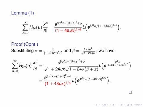
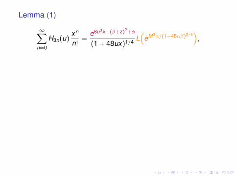
Lemma (1)
∞∑n=0
H3n(u)xn
n!=
e8u3x−(β+z)2+φ
(1 + 48ux)1/4 L(
eM3α/(1−48αβ)3/4),
where α = x(1+24xu)3/2 , β = 12xu2
√1+24xu
, z is a solution of
12αz2 + (24αβ − 1)z + 12αβ2 = 0, andφ = 2βz − 8αβ3 − 24αβ2z ++2z2 − 24αβz2 − 8αz3.

Theorem
∞∑n=0
H3n(u)xn
n!=
e8v3x+144v4x2
(1 + 48ux)1/4
∞∑n=0
(−1)n (6n)!(3n)! (1 + 48ux)3n/2
x2n
(2n)!,
where v = (√
1 + 48ux − 1)/(24x).
Lemma (1)
∞∑n=0
H3n(u)xn
n!=
e8u3x−(β+z)2+φ
(1 + 48ux)1/4 L(
eM3α/(1−48αβ)3/4),
where α = x(1+24xu)3/2 , β = 12xu2
√1+24xu
, z is a solution of
12αz2 + (24αβ − 1)z + 12αβ2 = 0, andφ = 2βz − 8αβ3 − 24αβ2z ++2z2 − 24αβz2 − 8αz3.

Lemma (1)
∞∑n=0
H3n(u)xn
n!=
e8u3x−(β+z)2+φ
(1 + 48ux)1/4 L(
eM3α/(1−48αβ)3/4).
Proof.For any positive integer ω,
∞∑n=0
Hωn(u)xn
n!= L
(e(M+2u)ωx).
So,
∞∑n=0
H3n(u)xn
n!= L
(e(M+2u)3x)
= e8u3xL(e6uxM2exM3+12u2xM).

Lemma (1)
∞∑n=0
H3n(u)xn
n!=
e8u3x−(β+z)2+φ
(1 + 48ux)1/4 L(
eM3α/(1−48αβ)3/4).
Proof.For any positive integer ω,
∞∑n=0
Hωn(u)xn
n!= L
(e(M+2u)ωx).
So,
∞∑n=0
H3n(u)xn
n!= L
(e(M+2u)3x)
= e8u3xL(e6uxM2exM3+12u2xM).

Lemma (1)
∞∑n=0
H3n(u)xn
n!=
e8u3x−(β+z)2+φ
(1 + 48ux)1/4 L(
eM3α/(1−48αβ)3/4).
Proof (Cont.)If f (M) is a power series and γ is a function not dependent onM, then
L(eγM2
f (M))=
1√1 + 4γ
L(
f( M√
1 + 4γ
)).
Thus,
∞∑n=0
H3n(u)xn
n!= e8u3xL(e6uxM2
exM3+12xu2M)
=e8u3x
√1 + 24ux
L(
ex
(1+24ux)3/2 M3+ 12u2x√1+24ux
M).

Lemma (1)
∞∑n=0
H3n(u)xn
n!=
e8u3x−(β+z)2+φ
(1 + 48ux)1/4 L(
eM3α/(1−48αβ)3/4).
Proof (Cont.)For α and β functions not dependent on M,
L(eαM3+βM) =e−(β+z)2+φ√
1− 24α(β + z)L(e
M3α(1−24α(β+z))3/2
),
where φ = 2βz − 8αβ3 − 24αβ2z + 2z2 − 24αβz2 − 8αz3, andz is a solution of 12αz2 + (24αβ − 1)z + 12αβ2 = 0.

Lemma (1)
∞∑n=0
H3n(u)xn
n!=
e8u3x−(β+z)2+φ
(1 + 48ux)1/4 L(
eM3α/(1−48αβ)3/4).
Proof (Cont.)
L(eαM3+βM) =e−(β+z)2+φ√
1− 24α(β + z)L(e
M3α(1−24α(β+z))3/2
).
Hence,
∞∑n=0
H3n(u)xn
n!=
e8u3x√
1 + 24uxL(
ex
(1+24ux)3/2 M3+ 12u2x√1+24ux
M)=
e8u3x−(β+z)2+φ
√1 + 24ux
√1− 24α(β + z)
L(
eM3α
(1−24α(β+z))3/2).

Lemma (1)
∞∑n=0
H3n(u)xn
n!=
e8u3x−(β+z)2+φ
(1 + 48ux)1/4 L(
eM3α/(1−48αβ)3/4).
Proof (Cont.)Substituting α = x
(1+24xu)3/2 and β = 12xu2√
1+24xu,
we have
∞∑n=0
H3n(u)xn
n!=
e8u3x−(β+z)2+φ
√1 + 24ux
√1− 24α(β + z)
L(
eM3α
(1−24α(β+z))3/2)
=e8u3x−(β+z)2+φ
(1 + 48ux)1/4 L(
eM3α/(1−48αβ)3/4).
Lemma (1)
∞∑n=0
H3n(u)xn
n!=
e8u3x−(β+z)2+φ
(1 + 48ux)1/4 L(
eM3α/(1−48αβ)3/4).
Proof (Cont.)Substituting α = x
(1+24xu)3/2 and β = 12xu2√
1+24xu, we have
∞∑n=0
H3n(u)xn
n!=
e8u3x−(β+z)2+φ
√1 + 24ux
√1− 24α(β + z)
L(
eM3α
(1−24α(β+z))3/2)
=e8u3x−(β+z)2+φ
(1 + 48ux)1/4 L(
eM3α/(1−48αβ)3/4).

Theorem
∞∑n=0
H3n(u)xn
n!=
e8v3x+144v4x2
(1 + 48ux)1/4
∞∑n=0
(−1)n (6n)!(3n)! (1 + 48ux)3n/2
x2n
(2n)!,
where v = (√
1 + 48ux − 1)/(24x).
Lemma (1)
∞∑n=0
H3n(u)xn
n!=
e8u3x−(β+z)2+φ
(1 + 48ux)1/4 L(
eM3α/(1−48αβ)3/4),
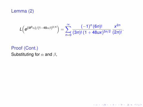
Lemma (2)
L(
e(M3α)/(1−48αβ)3/4)=∞∑
n=0
(−1)n (6n)!(3n)! (1 + 48ux)3n/2
x2n
(2n)!.

Theorem
∞∑n=0
H3n(u)xn
n!=
e8v3x+144v4x2
(1 + 48ux)1/4
∞∑n=0
(−1)n (6n)!(3n)! (1 + 48ux)3n/2
x2n
(2n)!,
where v = (√
1 + 48ux − 1)/(24x).
Lemma (1)
∞∑n=0
H3n(u)xn
n!=
e8u3x−(β+z)2+φ
(1 + 48ux)1/4 L(
eM3α/(1−48αβ)3/4),
Lemma (2)
L(
e(M3α)/(1−48αβ)3/4)=∞∑
n=0
(−1)n (6n)!(3n)! (1 + 48ux)3n/2
x2n
(2n)!.

Lemma (2)
L(
e(M3α)/(1−48αβ)3/4)=∞∑
n=0
(−1)n (6n)!(3n)! (1 + 48ux)3n/2
x2n
(2n)!.
Proof.Using the series expansion of ex ,
we have
L(
e(M3α)/(1−48αβ)3/4)
= L( ∞∑
n=0
1n!·( M3α
(1− 48αβ)3/4
)n)
= L( ∞∑
n=0
M3n αn
n! (1− 48αβ)3n/4
).

Lemma (2)
L(
e(M3α)/(1−48αβ)3/4)=∞∑
n=0
(−1)n (6n)!(3n)! (1 + 48ux)3n/2
x2n
(2n)!.
Proof.Using the series expansion of ex , we have
L(
e(M3α)/(1−48αβ)3/4)
= L( ∞∑
n=0
1n!·( M3α
(1− 48αβ)3/4
)n)
= L( ∞∑
n=0
M3n αn
n! (1− 48αβ)3n/4
).

Lemma (2)
L(
e(M3α)/(1−48αβ)3/4)=∞∑
n=0
(−1)n (6n)!(3n)! (1 + 48ux)3n/2
x2n
(2n)!.
Proof (Cont.)Since L is linear over umbrae,
L(
e(M3α)/(1−48αβ)3/4)= L
( ∞∑n=0
M3n αn
n! (1− 48αβ)3n/4
)
=∞∑
n=0
L(M3n) αn
n! (1− 48αβ)3n/4 .

Lemma (2)
L(
e(M3α)/(1−48αβ)3/4)=∞∑
n=0
(−1)n (6n)!(3n)! (1 + 48ux)3n/2
x2n
(2n)!.
Proof (Cont.)Since L is linear over umbrae,
L(
e(M3α)/(1−48αβ)3/4)= L
( ∞∑n=0
M3n αn
n! (1− 48αβ)3n/4
)
=∞∑
n=0
L(M3n) αn
n! (1− 48αβ)3n/4 .

Lemma (2)
L(
e(M3α)/(1−48αβ)3/4)=∞∑
n=0
(−1)n (6n)!(3n)! (1 + 48ux)3n/2
x2n
(2n)!.
Proof (Cont.)Since L
(M2n+1) = 0 and L
(M2n) = (−1)n(2n)!
n! ,
L(
e(M3α)/(1−48αβ)3/4)=∞∑
n=0
L(M3n) αn
n! (1− 48αβ)3n/4
=∞∑
n=0
L(M6n) α2n
(2n)! (1− 48αβ)3n/2
=∞∑
n=0
(−1)3n(6n)!(3n)!
· α2n
(2n)!(1− 48αβ)3n/2 .

Lemma (2)
L(
e(M3α)/(1−48αβ)3/4)=∞∑
n=0
(−1)n (6n)!(3n)! (1 + 48ux)3n/2
x2n
(2n)!.
Proof (Cont.)Since L
(M2n+1) = 0 and L
(M2n) = (−1)n(2n)!
n! ,
L(
e(M3α)/(1−48αβ)3/4)=∞∑
n=0
L(M3n) αn
n! (1− 48αβ)3n/4
=∞∑
n=0
L(M6n) α2n
(2n)! (1− 48αβ)3n/2
=∞∑
n=0
(−1)3n(6n)!(3n)!
· α2n
(2n)!(1− 48αβ)3n/2 .
Lemma (2)
L(
e(M3α)/(1−48αβ)3/4)=∞∑
n=0
(−1)n (6n)!(3n)! (1 + 48ux)3n/2
x2n
(2n)!.
Proof (Cont.)Substituting for α and β,
we have
L(
e(M3α)/(1−48αβ)3/4)=∞∑
n=0
(−1)3n(6n)!(3n)!
· α2n
(2n)!(1− 48αβ)3n/2
=∞∑
n=0
(−1)n (6n)!(3n)! (1 + 48ux)3n/2
x2n
(2n)!.

Lemma (2)
L(
e(M3α)/(1−48αβ)3/4)=∞∑
n=0
(−1)n (6n)!(3n)! (1 + 48ux)3n/2
x2n
(2n)!.
Proof (Cont.)Substituting for α and β, we have
L(
e(M3α)/(1−48αβ)3/4)=∞∑
n=0
(−1)3n(6n)!(3n)!
· α2n
(2n)!(1− 48αβ)3n/2
=∞∑
n=0
(−1)n (6n)!(3n)! (1 + 48ux)3n/2
x2n
(2n)!.

Theorem
∞∑n=0
H3n(u)xn
n!=
e8v3x+144v4x2
(1 + 48ux)1/4
∞∑n=0
(−1)n (6n)!(3n)! (1 + 48ux)3n/2
x2n
(2n)!,
where v = (√
1 + 48ux − 1)/(24x).
Lemma (1 & 2)
∞∑n=0
H3n(u)xn
n!=
e8u3x−(β+z)2+φ
(1 + 48ux)1/4
∞∑n=0
(−1)n (6n)!(3n)! (1 + 48ux)3n/2
x2n
(2n)!.
Lemma (3)
e8u3x−(β+z)2+φ = e8v3x+144v4x2,
where v = (√
1 + 48ux − 1)/(24x).

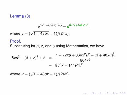
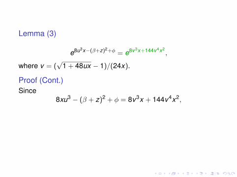
Lemma (3)
e8u3x−(β+z)2+φ = e8v3x+144v4x2,
where v = (√
1 + 48ux − 1)/(24x).
Proof.Substituting for β, z, and φ using Mathematica,
we have
8xu3 − (β + z)2 + φ =1 + 72xu + 864x2u2 − (1 + 48xu)
32
864x2
= 8v3x + 144v4x2
where v = (√
1 + 48ux − 1)/(24x).
Lemma (3)
e8u3x−(β+z)2+φ = e8v3x+144v4x2,
where v = (√
1 + 48ux − 1)/(24x).
Proof.Substituting for β, z, and φ using Mathematica, we have
8xu3 − (β + z)2 + φ =1 + 72xu + 864x2u2 − (1 + 48xu)
32
864x2
= 8v3x + 144v4x2
where v = (√
1 + 48ux − 1)/(24x).
Lemma (3)
e8u3x−(β+z)2+φ = e8v3x+144v4x2,
where v = (√
1 + 48ux − 1)/(24x).
Proof (Cont.)Since
8xu3 − (β + z)2 + φ = 8v3x + 144v4x2,
e8u3x−(β+z)2+φ = e8v3x+144v4x2

Lemma (3)
e8u3x−(β+z)2+φ = e8v3x+144v4x2,
where v = (√
1 + 48ux − 1)/(24x).
Proof (Cont.)Since
8xu3 − (β + z)2 + φ = 8v3x + 144v4x2,
e8u3x−(β+z)2+φ = e8v3x+144v4x2
Lemma (1)
∞∑n=0
H3n(u)xn
n!=
e8u3x−(β+z)2+φ
(1 + 48ux)1/4 L(
eM3α/(1−48αβ)3/4),
Lemma (2)
L(
e(M3α)/(1−48αβ)3/4)=∞∑
n=0
(−1)n (6n)!(3n)! (1 + 48ux)3n/2
x2n
(2n)!.
Lemma (3)
e8u3x−(β+z)2+φ = e8v3x+144v4x2,
where v = (√
1 + 48ux − 1)/(24x).

Lemma (1)
∞∑n=0
H3n(u)xn
n!=
e8u3x−(β+z)2+φ
(1 + 48ux)1/4 L(
eM3α/(1−48αβ)3/4),
Lemma (2)
L(
e(M3α)/(1−48αβ)3/4)=∞∑
n=0
(−1)n (6n)!(3n)! (1 + 48ux)3n/2
x2n
(2n)!.
Lemma (3)
e8u3x−(β+z)2+φ = e8v3x+144v4x2,
where v = (√
1 + 48ux − 1)/(24x).

Lemma (1)
∞∑n=0
H3n(u)xn
n!=
e8u3x−(β+z)2+φ
(1 + 48ux)1/4 L(
eM3α/(1−48αβ)3/4),
Lemma (2)
L(
e(M3α)/(1−48αβ)3/4)=∞∑
n=0
(−1)n (6n)!(3n)! (1 + 48ux)3n/2
x2n
(2n)!.
Lemma (3)
e8u3x−(β+z)2+φ = e8v3x+144v4x2,
where v = (√
1 + 48ux − 1)/(24x).

Further Applications
Theorem
∞∑n=0
H3n(u)xn
n!=
e8v3x+144v4x2
(1 + 48ux)1/4
∞∑n=0
(−1)n (6n)!(3n)! (1 + 48ux)3n/2
x2n
(2n)!,
where v = (√
1 + 48ux − 1)/(24x).
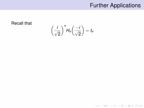
Further Applications
Recall that (i√2
)n
Hn
(−i√
2
)= tn
Corollary
∞∑n=0
t3nxn
n!=
e−4w3x√
2−72w4x2
(1 + 24x)1/4
∞∑n=0
(6n)!(3n)! (1 + 24x)3n/2
x2n
(2n)!2n ,
where
w =
√2(√
1 + 24x − 1)24x
.

Further Applications
Recall that (i√2
)n
Hn
(−i√
2
)= tn
Corollary
∞∑n=0
t3nxn
n!=
e−4w3x√
2−72w4x2
(1 + 24x)1/4
∞∑n=0
(6n)!(3n)! (1 + 24x)3n/2
x2n
(2n)!2n ,
where
w =
√2(√
1 + 24x − 1)24x
.

References
I.M. Gessel.Applications of the Classical Umbral Calculus.Algebra univers., 49 (2003), 397–434.
V. De Angelis.Class Lecture, The Umbral Calculus.Louisiana State University, Baton Rouge, LA.Summer 2013.

Acknowledgements
Ben Warren and Dr. Valerio De Angelis


![Umbral Calculus - arXiv.org e-Print archive · 2018-03-09 · side operational calculus [101] and into the methods introduced by the oper- ationalists (Sylvester, Boole, Glaisher,](https://static.fdocuments.us/doc/165x107/5f2e44aa00e8eb02c77dab01/umbral-calculus-arxivorg-e-print-archive-2018-03-09-side-operational-calculus.jpg)


