Tecplot 360 Data Format Guide - ustc.edu.cnhome.ustc.edu.cn/~cbq/360_data_format_guide.pdf · ·...
164
Tecplot, Inc. Bellevue, WA 2015 Data Format Guide Tecplot 360 EX 2015 Release 1
Transcript of Tecplot 360 Data Format Guide - ustc.edu.cnhome.ustc.edu.cn/~cbq/360_data_format_guide.pdf · ·...

Tecplot, Inc. Bellevue, WA 2015
Data Format Guide
Tecplot 360 EX 2015 Release 1

Tecplot 360 EX Data Format Guide is for use with Tecplot 360 EX 2015 R1.
Copyright © 1988-2015 Tecplot, Inc. All rights reserved worldwide. Except for personal use, this manual may not be reproduced, transmitted, transcribed,stored in a retrieval system, or translated in any form, in whole or in part, without the express written permission of Tecplot, Inc., 3535 Factoria Blvd, Ste. 550;Bellevue, WA 98006 U.S.A.
The software discussed in this documentation and the documentation itself are furnished under license for utilization and duplication only according to thelicense terms. The copyright for the software is held by Tecplot, Inc. Documentation is provided for information only. It is subject to change without notice. Itshould not be interpreted as a commitment by Tecplot, Inc. Tecplot, Inc. assumes no liability or responsibility for documentation errors or inaccuracies.
Tecplot, Inc.Post Office Box 52708Bellevue, WA 98015-2708 U.S.A.
Tel:1.800.763.7005 (within the U.S. or Canada), 00 1 (425)653-1200 (internationally)
email: [email protected], [email protected], comments or concerns regarding this document: [email protected]
For more information, visit http://www.tecplot.com
Tecplot®, Tecplot 360,™ Tecplot 360 EX,™ Tecplot Focus, the Tecplot product logos, Preplot,™ Enjoy the View,™ Master the View,™ SZL,™ Sizzle,™ andFramer™ are registered trademarks or trademarks of Tecplot, Inc. in the United States and other countries. All other product names mentioned herein aretrademarks or registered trademarks of their respective owners.
NOTICE TO U.S. GOVERNMENT END-USERS
Use, duplication, or disclosure by the U.S. Government is subject to restrictions as set forth in subparagraphs (a) through (d) of the Commercial Computer-Restricted Rights clause at FAR 52.227-19 when applicable, or in subparagraph (c)(1)(ii) of the Rights in Technical Data and Computer Software clause atDFARS 252.227-7013, and/or in similar or successor clauses in the DOD or NASA FAR Supplement. Contractor/manufacturer is Tecplot, Inc., 3535 FactoriaBlvd, Ste. 550; Bellevue, WA 98006 U.S.A.
15-360-05-1
Rev 1/2015
For third-party trademark and copyright information, see the Tecplot 360 EX User’s Manual.

3
Table of Contents
1 Introduction ............................................................................ 7
Subzone Loading ..........................................................................7Creating Data Files for Tecplot 360 & Tecplot Focus...............8Best Practices .................................................................................8
2 Data Structure .................................................................... 11
Ordered Data............................................................................... 12Finite Element Data .................................................................... 12
Line Data ................................................................................. 14Surface Data ............................................................................. 14Volume Data ............................................................................. 14Finite Element Data Limitations................................................. 15
Variable Location ........................................................................ 15Face Neighbors............................................................................ 16Working with Unorganized Data Sets..................................... 16
Example - Unorganized Three-Dimensional Volume ..................... 17Time and Date Representation ................................................. 18
3 Binary Data ............................................................................ 19
Getting Started ............................................................................ 19Viewing Your Output................................................................. 20Binary File Compatibility .......................................................... 20
Deprecated Binary Functions ..................................................... 21Character Strings in FORTRAN ................................................ 21Boolean Flags ............................................................................ 21
Binary Data File Function Calling Sequence .......................... 21Writing to Multiple Binary Data Files...................................... 22

Table of Contents
4
Linking with the TecIO Library................................................ 22Linux/Macintosh....................................................................... 22Windows .................................................................................. 22Notes for Windows Programmers using Fortran .......................... 23
Binary Data File Function Reference ....................................... 23Defining Polyhedral and Polygonal Data ............................... 52
Boundary Faces and Boundary Connections ................................ 52FaceNodeCounts and FaceNodes................................................. 53FaceRightElems and FaceLeftElems ............................................ 54FaceBoundaryConnectionElements and Zones ............................. 55Partially Obscured Boundary Faces ............................................ 55
Examples...................................................................................... 56Face Neighbors.......................................................................... 56Polygonal Example.................................................................... 63Multiple Polyhedral Zones ......................................................... 68Multiple Polygonal Zones .......................................................... 80Polyhedral Example................................................................... 93IJ-ordered zone .......................................................................... 96Switching Between Two Files ..................................................... 99Text Example .......................................................................... 102
4 ASCII Data ........................................................................... 105
Converting ASCII to Binary .................................................... 105Syntax Rules & Limits.............................................................. 105ASCII File Structure ................................................................. 106
File Header ............................................................................. 106Zone Record ........................................................................... 107Text Record............................................................................. 116Geometry Record..................................................................... 119Custom Labels Record.............................................................. 122Data Set Auxiliary Data Record ............................................... 122Variable Auxiliary Data Record ................................................ 123ASCII Data File Parameter Assignment Values ......................... 123
Ordered Data............................................................................. 124I-Ordered Data ....................................................................... 124IJ-Ordered Data ...................................................................... 124IJK-Ordered Data .................................................................... 125Ordered Data Examples ........................................................... 125
Finite Element Data .................................................................. 130Variable and Connectivity List Sharing ..................................... 132Finite Element Data Set Examples ............................................ 134
ASCII Data File Conversion to Binary................................... 144Preplot Options....................................................................... 145Preplot Examples .................................................................... 145

5
5 Glossary ................................................................................. 147
A Binary Data File Format ............................................. 151

Table of Contents
6
7
1
Introduction
Tecplot 360 can read in data produced in many different formats using the data loaders provided with the product. This manual describes a complementary approach: writing your data in the Tecplot 360 data format so it can be read natively, providing the best experience for Tecplot 360 users.This Data Format Guide includes the following topics:
• Chapter 2: “Data Structure” Learn about the different types of data structure available in Tecplot 360 and how to use them.
• Chapter 3: “Binary Data” Refer to this chapter for details on outputting data in Tecplot 360’s binary file format (.plt) or the newer subzone load format (.szplt) using the TecIO library, a collection of routines we provide that you can use to write files in these format from your software.
• Chapter 4: “ASCII Data” We strongly recommend that you create binary data files. However, we provide the ASCII data chapter to allow you to create simple data files.
• Chapter 5: “Glossary” Refer to the Glossary for the definitions of terms used throughout the manual.
• The Appendix, Binary Data File Format, documents the .plt binary file format.
1 - 1 Subzone LoadingTecplot 360 EX introduced a new subzone loadable file format with extension .szplt that is optimized for loading partial zones (“subzones”) as individual chunks of data are needed for a plot or for other operations. Subzone loading improves performance substantially for large cases while reducing RAM usage. If your software generates large data files, we strongly encourage you to support this format, as it will significantly improve your user experience. The API is the same as is used to write .plt files, so if your program already uses TecIO, it is straightforward to upgrade it to write .szplt files instead of, or in addition to, .plt files.
Before continuing to either the Binary or ASCII chapter, please review this overview of Best Practices.

8
1 - 2 Creating Data Files for Tecplot 360 & Tecplot Focus
If you intend to create data files that will load in both Tecplot 360 and Tecplot Focus, you need to be aware that polyhedral/polygonal zones are not supported in Tecplot Focus. If any of the zones in a given data file are polyhedral, you will not be able to load the data file into Tecplot Focus. To create data files that will load in both products, you must use either ordered zones or cell-based finite element zones (triangular, quadrilateral, tetrahedral or brick elements).
The subzone load file format (.szplt) is not supported by Tecplot Focus, nor by legacy versions of Tecplot 360 (versions without “EX” in their designation).
1 - 3 Best PracticesUsers who wish to generate native Tecplot 360 data files automatically from applications such as complex flow solvers have a number of options for outputting data into Tecplot’s data format. This section outlines a few "best practices" for outputting your data into Tecplot 360 data format.
1. Offer the Option to Write Subzone Load Files (.szplt)Users of Tecplot 360 EX will appreciate the improved experience provided by these files, especially for large cases.
2. Create Binary Data Files (.plt or .szplt) instead of ASCII (.dat)Binary data files are more efficient than ASCII files, in terms of disk space and time to first image. To create binary data files, you may use functions provided in the TecIO library. To create ASCII files, you can write out plain text in the usual manner. There are some cases where ASCII files are preferred. Create ASCII files when:
• Your data files are small.• Your application runs on a platform for which the TecIO library is not provided. Even if
this is the case, please contact us at [email protected]. There may be a way to resolve this issue.
• You wish users to be able to view or edit the data in a text editor.3. Use Block Format instead of Point Format
Block format is by far the most efficient format when it comes to loading the file into Tecplot 360. If your data files are small and you can only obtain the data in a point-like format (for example, with a spreadsheet), then using point format is acceptable.
4. Use the Native Byte Ordering for the Target Machine When you create binary data, you can elect to produce these files in either Motorola byte order or Intel byte order. Today’s most popular platforms all use Intel byte order, and generally this is the order you should use when writing binary data. The exceptions involve older platforms no longer supported by Tecplot. If you are using such legacy platforms, be sure to write the binary data in the order native to the platform on which it will be viewed.
For the purposes of this discussion, “polyhedral” refers to either polyhedral or polygonal zones.
Binary files can only be written in block format. Point format is allowed for ASCII files, but running the preplot utility will convert the data to block format.

9
Best Practices
While Tecplot 360 automatically detects the byte order and loads either format, it is more efficient if the file uses the byte order used on the platform where you run Tecplot 360. For See the notes about this option in Section B - 3 “Preplot” in the User’s Manual for the Preplot flag.
5. Add Auxiliary data to Preset Variable Assignments in Tecplot 360Zone Auxiliary data can be used to give Tecplot 360 hints about properties of your data. For example, it can be used to set the defaults for which variables to use for certain kinds of plots. Auxiliary data is supported by both binary and ASCII formats. Refer to Section “TECAUXSTR142” on page 23 or Section 4 - 3.6 “Data Set Auxiliary Data Record” for information on working with auxiliary data in binary or ASCII data files, respectively.
6. Data SharingShare variables whenever possible. Variable sharing is commonly used for the spatial variables (X, Y, and Z) when you have many sets of data that use the same basic grid. This saves disk space, as well as memory when the data is loaded into Tecplot 360. In addition, the benefits are compounded with scratch data derived from these variables because it is also shared within Tecplot 360. See also Section “TECZNE142” on page 47 (for binary data) or Section 4 - 5.1 “Variable and Connectivity List Sharing” (for ASCII data).
7. Passive VariablesTecplot 360 can manage many data sets at the same time. However, within a given data set you must supply the same number of variables for each zone. In some cases you may have data where there are many variables and, for some of the zones some of those variables are not important. If that is the case, you can set selected variables in those zones to be passive. A passive variable is one that will always return the value zero if queried (e.g. in a probe) but will not involve itself in operations such as the calculations of the min and max range. This is very useful when calculating default contour levels.

10

11
2
Data Structure
Tecplot 360 accommodates two different types of data: Ordered Data and Finite Element Data.
A connectivity list is used to define which nodes are included in each element of an ordered or cell-based finite element zone. You should know your zone type and the number of elements in each zone in order to create your connectivity list.
The number of nodes required for each element is implied by your zone type. For example, if you have a finite element quadrilateral zone, you will have four nodes defined for each element. Likewise, you must provide eight numbers for each cell in a BRICK zone, and three numbers for each element in a TRIANGLE zone. If you have a cell that has a smaller number of nodes than that required by your zone type, simply repeat a node number. For example, if you are working with a finite element quadrilateral zone and you would like to create a triangular element, simply repeat a node in the list (e.g., 1,4,5,5).
In the example below, the zone contains two quadrilateral elements. Therefore, the connectivity list must have eight values. The first four values define the nodes that form Element 1. Similarly, the second four values define the nodes that form Element 2.
The connectivity list for this example would appear as follows:
ConnList[8] = {4,5,2,1, /* nodes for Element 1 */ 5,6,3,2}; /* nodes for Element 2 */
It is important to provide your node list in either a clockwise or counter-clockwise order. Otherwise, your cell will twist, and the element produced will be misshapen.

12
2 - 1 Ordered DataOrdered data is defined by one, two, or three-dimensional logical arrays, dimensioned by IMAX, JMAX, and KMAX. These arrays define the interconnections between nodes and cells. The variables can be either nodal or cell-centered. Nodal variables are stored at the nodes; cell-centered values are stored within the cells.
• One-dimensional Ordered Data (I-ordered, J-ordered, or K-ordered)
• Two-dimensional Ordered Data (IJ-ordered, JK-ordered, IK-ordered)
• Three-dimensional Ordered Data (IJK-ordered)
2 - 2 Finite Element DataWhile finite element data is usually associated with numerical analysis for modeling complex problems in 3D structures (heat transfer, fluid dynamics, and electromagnetics), it also provides an effective approach for organizing data points in or around complex geometrical shapes. For example, you may not have the
A single dimensional array where either IMAX, JMAX or KMAX is greater than or equal to one, and the others are equal to one. For nodal data, the number of stored values is equal to IMAX * JMAX * KMAX. For cell-centered I-ordered data (where IMAX is greater than one, and JMAX and KMAX are equal to one), the number of stored values is (IMAX-1) - similarly for J-ordered and K-ordered data.
A two-dimensional array where two of the three dimensions (IMAX, JMAX, KMAX) are greater than one, and the other dimension is equal to one. For nodal data, the number of stored values is equal to IMAX * JMAX * KMAX. For cell-centered IJ-ordered data (where IMAX and JMAX are greater than one, and KMAX is equal to one), the number of stored values is (IMAX-1)(JMAX-1) - similarly for JK-ordered and IK-ordered data.
A three-dimensional array where all IMAX, JMAX and KMAX are each greater than one. For nodal ordered data, the number of nodes is the product of the I-, J-, and K-dimensions. For nodal data, the number of stored values is equal to IMAX * JMAX * KMAX. For cell-centered data, the number of stored values is (IMAX-1)(JMAX-1)(KMAX-1).

13
Finite Element Data
same number of data points on different lines, there may be holes in the middle of the dataset, or the data points may be irregularly (randomly) positioned. For such difficult cases, you may be able to organize your data as a patchwork of elements. Each element can be independent of the other elements, so you can group your elements to fit complex boundaries and leave voids within sets of elements. The figure below shows how finite element data can be used to model a complex boundary.
Figure 2-1. This figure shows finite element data used to model a complex boundary. This plot file, feexchng.plt, is located in your Tecplot 360 distribution under the examples/2D subdirectory.
Finite element data defines a set of points (nodes) and the connected elements of these points. The variables may be defined either at the nodes or at the cell (element) center. Finite element data can be divided into three types:
• Line data is a set of line segments defining a 2D or 3D line. Unlike I-ordered data, a single finite element line zone may consist of multiple disconnected sections. The values of the variables at each data point (node) are entered in the data file similarly to I-ordered data, where the nodes are numbered with the I-index. This data is followed by another set of data defining connections between nodes. This second section is often referred to as the connectivity list. All elements are lines consisting of two nodes, specified in the connectivity list.
• Surface data is a set of triangular, quadrilateral, or polygonal elements defining a 2D field or a 3D surface. When using polygonal elements, the number of sides may vary from element to element. In finite element surface data, you can choose (by zone) to arrange your data in three point (triangle), four point (quadrilateral), or variable-point (polygonal) elements. The number of points per node and their arrangement are determined by the element type of the zone. If a mixture of quadrilaterals and triangles is necessary, you may repeat a node in the quadrilateral element type to create a triangle, or you may use polygonal elements.
• Volume data is a set of tetrahedral, brick or polyhedral elements defining a 3D volume field. When using polyhedral elements, the number of sides may vary from element to element. Finite element volume cells may contain four points (tetrahedron), eight points (brick), or variable points (polyhedral). The figure below shows the arrangement of the nodes for

14
tetrahedral and brick elements. The connectivity arrangement for polyhedral data is governed by the method in which the polyhedral facemap data is supplied.
Figure 2-2. Connectivity arrangements for FE-volume datasetsIn the brick format, points may be repeated to achieve 4, 5, 6, or 7 point elements. For example, a connectivity list of “n1 n1 n1 n1 n5 n6 n7 n8” (where n1 is repeated four times) results in a quadrilateral-based pyramid element. Section 4 - 5 “Finite Element Data” in the Data Format Guide provides detailed information about how to format your FE data in Tecplot’s data file format.
2 - 2.1 Line DataUnlike I-ordered data, a single finite element line zone may consist of multiple disconnected sections. The values of the variables at each data point (node) are entered in the data file similarly to I-ordered data, where the nodes are numbered with the I-index. This data is followed by another set of data defining connections between nodes. This second section is often referred to as the connectivity list. All elements are lines consisting of two nodes, specified in the connectivity list.
2 - 2.2 Surface DataIn finite element surface data, you can choose (by zone) to arrange your data in three point (triangle), four point (quadrilateral), or variable-point (polygonal) elements. The number of points per node and their arrangement are determined by the element type of the zone. If a mixture of quadrilaterals and triangles is necessary, you may repeat a node in the quadrilateral element type to create a triangle or you may use polygonal elements.
2 - 2.3 Volume Data• Finite element volume cells may contain four points (tetrahedron),eight points (brick) or a variable
number of points (polyhedral). The figure below shows the arrangement of the nodes for tetrahedral and
Tetrahedral connectivity arrangement Brick connectivity arrangement

15
Variable Location
brick elements. The connectivity arrangement for polyhedral data is governed by the method in which the polyhedral facemap data is supplied.
Figure 2-3. Connectivity arrangements for FE-volume datasetsIn the brick format, points may be repeated to achieve 4, 5, 6, or 7 point elements. For example, a connectivity list of “n1 n1 n1 n1 n5 n6 n7 n8” (where n1 is repeated four times) results in a quadrilateral-based pyramid element.
2 - 2.4 Finite Element Data LimitationsWorking with finite element data has some limitations:
• XY-plots of finite element data treat the data as I-ordered; that is, the connectivity list is ignored. Only nodes are plotted, not elements, and the nodes are plotted in the order in which they appear in the data file.
• Index skipping in vector and scatter plots treats finite element data as I-ordered; the connectivity list is ignored. Nodes are skipped according to their order in the data file.
2 - 3 Variable LocationData values can be stored at the nodes or at the cell centers.
• For finite element meshes, cell-centers are the centers (centroids) of elements. • For many types of plots, cell-centered values are interpolated to the nodes internally.
Tetrahedral connectivity arrangement Brick connectivity arrangement

16
2 - 4 Face NeighborsA cell is considered a neighbor if one of its faces shares all nodes in common with the selected cell, or if it is identified as a neighbor by face neighbor data in the dataset. The face numbers for cells in the various zone types are defined below.
Figure 2-1. A: Example of node and face neighbors for an FE-brick cell or IJK-ordered cell. B: Example of node and face numbering for an IJ-ordered/ FE-quadrilateral cell. C: Example of tetrahedron face neighbors.
The implicit connections between elements in a zone may be overridden, or connections between cells in adjacent zones established by specifying face neighbor criteria in the data file. Refer to Section “TECFACE142” on page 26 for additional information.
2 - 5 Working with Unorganized Data SetsTecplot 360 loads unorganized data as a single I-ordered zone and displays them in XY Mode, by default. Tecplot products consider an I-ordered zone irregular if it has more than one dependent variable. An I-ordered data set with one dependent variable (i.e. an XY or polar line) is NOT an irregular zone.
To check for irregular data, you can go to the Data>Data Set Info dialog (accessed via the Data menu). The values assigned to: IMax, JMax, and KMax are displayed in the lower left quadrant of that dialog. If IMax is greater than 1, and JMax and KMax are equal to 1, then your data is irregular.
It is also easy to tell if you have irregular data by looking at the plot. If you are looking at irregular data with the Mesh layer turned on, the data points will be connected by lines in the order the points appear in the data set.
You can organize your data set for Tecplot 360 in one of the following ways.
1. Manually order the data file using a text editor.
2. Use one of the Data>Interpolation options. See Section 20 - 7 “Data Interpolation” in the Tecplot 360 User’s Manual.
A B C
Use the “Label Points and Cells” feature from the Plot menu to see if your data set can be easily corrected using a text editor by correcting the values for I, J, and/or K.

17
Working with Unorganized Data Sets
2 - 5.1 Example - Unorganized Three-Dimensional Volume To use 3D volume irregular data in field plots, you must interpolate the data onto a regular, IJK-ordered zone. To interpolate your data, perform the following steps:
1. Place your 3D volume irregular data into an I-ordered zone in a data file.2. Read in your data file and create a 3D scatter plot.3. From the Data menu, choose Create Zone>Rectangular. (Circular will also work.)4. In the Create Rectangular Zone dialog, enter the I-, J-, and K-dimensions for the new zone; at
a minimum, you should enter 10 for each dimension. The higher the dimensions, the finer the interpolation grid, but the longer the interpolating and plotting time.
5. Enter the minimum and maximum X, Y, and Z values for the new zone. The default values are the minimums and maximums of the current (irregular) dataset.
6. Click [Create] to create the new zone, and [Close] to dismiss the dialog.7. From the Data menu, choose Interpolate>Inverse Distance. (Linear also works.)8. In the Inverse-Distance Interpolation dialog, choose the irregular data zone as the source
zone, and the newly created IJK-ordered zone as the destination zone. Set any other parameters as desired
9. Select the [Compute] button to perform the interoplation.
Once the interpolation is complete, you can plot the new IJK-ordered zone as any other 3D volume zone. You may plot iso-surfaces, volume streamtraces, and so forth. At this point, you may want to deactivate or delete the original irregular zone so as not to conflict with plots of the new zone.
Figure 2-2 shows an example of irregular data interpolated into an IJK-ordered zone, with iso-surfaces plotted on the resultant zone.
Figure 2-2. Irregular data interpolated into an IJK-ordered zone.

18
2 - 6 Time and Date RepresentationTecplot 360 uses floating point numbers to represent times and dates. The integer portion represents the number of days since December 30, 1899. The decimal portion represents a fractional portion of a day. The table below illustrates some examples of this method.
Tecplot 360 supports dates from 1800-01-01 through 9999-12-31. This formatting matches the representation method used by Microsoft Excel, enabling you to load time/date data easily from Excel into Tecplot 360. However, because Excel software’s original formatting incorrectly calculated 1900 as a leap year, only dates from Mar 1, 1900 forward will import correctly into Tecplot 360.
Date Time Floating Point Number 1900-01-01 00:00:00 2.01900-01-01 12:00:00 2.52008-07-31 00:00:00 39660.0 2008-07-31 12:00:00 39660.5 2008-07-31 12:01:00 39660.5006944444 2008-07-31 13:00:00 39660.5416666667

19
3
Binary Data
This chapter is intended for experienced programmers who need to create Tecplot binary data files directly. Support for topics discussed in this chapter is limited to general questions about writing Tecplot binary files. It is beyond the scope of our Technical Support to offer programming advice and to debug programs. For additional help, visit http://www.tecplottalk.com.
It is easy to write ASCII files in text format, and they have the advantage that you can inspect them using a text editor to make sure they are being written correctly. Their primary disadvantages are that they can consume much more disk space than binary files and are slower to load, which is especially noticeable when they are large. While users can convert them to the binary format with the Preplot utility (see Section 4 - 1 “Converting ASCII to Binary” for additional information), it is much more efficient to simply write them in binary format to begin with.
To output your data directly into Tecplot’s basic binary file format, .plt, you may use the TecIO library, which is provided at no cost by Tecplot, Inc., or you may write your own binary functions. If you wish to write your own functions, refer to Appendix A: Section “Binary Data File Format” for details on the structure of .plt files. If you wish to link with the library provided by Tecplot, begin with Section 3 - 1 “Getting Started” and use Appendix A: Section “Binary Data File Format” only for reference.
If you wish to write files in the newer .szplt format, you must use the TecIO library.
3 - 1 Getting StartedTecIO is a static library of utility functions that you can link with your application to create binary data files directly, bypassing the use of ASCII files. This makes for fewer files to manage, conserves disk space, and saves the time required to convert the files.
TecIO supports two binary file formats:
• Tecplot Binary (.plt) - The legacy format written by versions of Tecplot 360 and Tecplot Focus prior to Tecplot 360 EX. It is of course also supported by Tecplot 360 EX.
You can find source files for most of the examples in this chapter in the examples/tecio folder of your Tecplot 360 EX installation.
20
• Tecplot Subzone Loadable (.szplt) - A newer format introduced with Tecplot 360 EX, optimized for large data sets, that enables substantially improved interactive performance for common workflows and a reduced memory footprint.
We encourage you to support both formats. Users of Tecplot 360 EX will appreciate the improved experience, while users of older versions of Tecplot 360, Tecplot Focus, and other programs that can read Tecplot-format binary files will appreciate being able to use your data with their software.
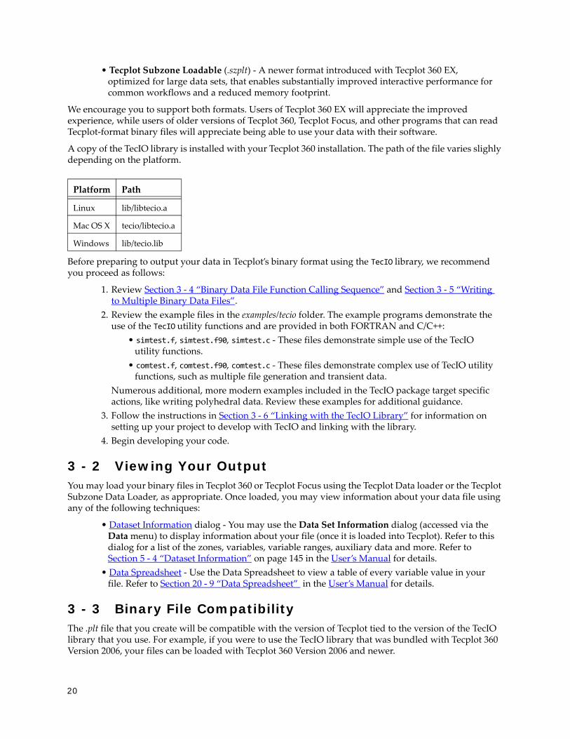
A copy of the TecIO library is installed with your Tecplot 360 installation. The path of the file varies slighly depending on the platform.
Before preparing to output your data in Tecplot’s binary format using the TecIO library, we recommend you proceed as follows:
1. Review Section 3 - 4 “Binary Data File Function Calling Sequence” and Section 3 - 5 “Writing to Multiple Binary Data Files”.
2. Review the example files in the examples/tecio folder. The example programs demonstrate the use of the TecIO utility functions and are provided in both FORTRAN and C/C++:
• simtest.f, simtest.f90, simtest.c - These files demonstrate simple use of the TecIO utility functions.
• comtest.f, comtest.f90, comtest.c - These files demonstrate complex use of TecIO utility functions, such as multiple file generation and transient data.
Numerous additional, more modern examples included in the TecIO package target specific actions, like writing polyhedral data. Review these examples for additional guidance.
3. Follow the instructions in Section 3 - 6 “Linking with the TecIO Library” for information on setting up your project to develop with TecIO and linking with the library.
4. Begin developing your code.
3 - 2 Viewing Your OutputYou may load your binary files in Tecplot 360 or Tecplot Focus using the Tecplot Data loader or the Tecplot Subzone Data Loader, as appropriate. Once loaded, you may view information about your data file using any of the following techniques:
• Dataset Information dialog - You may use the Data Set Information dialog (accessed via the Data menu) to display information about your file (once it is loaded into Tecplot). Refer to this dialog for a list of the zones, variables, variable ranges, auxiliary data and more. Refer to Section 5 - 4 “Dataset Information” on page 145 in the User’s Manual for details.
• Data Spreadsheet - Use the Data Spreadsheet to view a table of every variable value in your file. Refer to Section 20 - 9 “Data Spreadsheet” in the User’s Manual for details.
3 - 3 Binary File CompatibilityThe .plt file that you create will be compatible with the version of Tecplot tied to the version of the TecIO library that you use. For example, if you were to use the TecIO library that was bundled with Tecplot 360 Version 2006, your files can be loaded with Tecplot 360 Version 2006 and newer.
Platform Path
Linux lib/libtecio.a
Mac OS X tecio/libtecio.a
Windows lib/tecio.lib

21
Binary Data File Function Calling Sequence
This is independent of the version number used for the binary functions (for example, the 142 in TECZNE142). For example, even if you use 112 functions with the version of the TecIO library included with this distribution, your .plt file will be compatible with this version of Tecplot 360 and newer.
A .plt file is also backward compatible to the first version of Tecplot 360 or Focus that uses the file format version supported by the library being used. However, these older Tecplot products cannot read .szplt files regardless of their version.
Subzone data files (.szplt) can be loaded only in Tecplot 360 EX. At this writing, there is only one version of this file format. We anticipate a similar situation as with .plt files, however: future versions of Tecplot 360 EX (after the initial release, Tecplot 360 EX 2014 R1) will be able to read files created with older versions of the TecIO library, but future versions of Tecplot 360 EX may have features that require a new version of TecIO to write them, and these files may not be loadable by previous version of Tecplot 360 EX.
3 - 3.1 Deprecated Binary FunctionsFunctions whose names end in an integer less than 142 are deprecated and are provided only for compatibility with older code. We recommend you use the 142 binary function family with new code and/or if you need to update your application to take advantage of the new functionality provided with version 142. In order to use the 142 family of functions, use the TecIO library included in your Tecplot 360 2015 distribution. If you have existing code using deprecated functions, and want to use any binary function calls from version 142, you must update all your TecIO library calls to 142.
API version 142 or later allows applications to select between the .plt and .szplt file formats at runtime, a feature introduced with Tecplot 360 2014 R2. In Tecplot 360 2014 R1, two versions of the TecIO library were provided, one that wrote .plt files and one that wrote the new .szplt files. Both used version 142 functions and had identical APIs; the file format was determined solely by the version of the library linked with your application. In Tecplot 360 2014 R2 and later, a single library is provided, and a parameter was added to TECINI to choose the format when opening the file for writing (see TECINI142). The library always writes .plt files when using an API version before 142.
3 - 3.2 Character Strings in FORTRANAll character string parameters passed to TecIO must use C-style strings: that is, they must terminate with a null character. In FORTRAN, this can be done by concatenating char(0) to the end of a character string.
For example, to send the character string “Hi Mom” to a function called A, use the following syntax:
I=A("Hi Mom"//char(0))
3 - 3.3 Boolean FlagsInteger parameters identified as "flags" indicate boolean values. Pass 1 for true, and 0 for false.
3 - 4 Binary Data File Function Calling SequenceFor a given file, the binary data file functions must be called in a specific order. The order is as follows:
TECFOREIGN142 (Optional)TECINI142
For each call to TECINI142, use one or more of the following: TECAUXSTR142 (Optional)TECVAUXSTR142 (Optional)TECZNE142 (One or more to create multiple zones)
For each call to TECZNE142, use one of more of these:TECDAT142 (One or more to fill each zone)

22
TECNOD142 or TECNODE142 (One or more for each finite element zone)TECFACE142 (One for each zone with face connections)TECPOLY142 or TECPOLYFACE142/TECPOLYBCONN142 (Optional - polyhedral data)TECZAUXSTR142 (Optional)
TECLAB142 (Optional)TECGEO142 (Optional)TECTXT142 (Optional)
TECFIL142 (Optional - use if you are switching between files)TECUSR142 (Optional)TECEND142
Section 3 - 5 “Writing to Multiple Binary Data Files” explains how you can use the TECFIL142 function along with the above functions to write to multiple files simultaneously.
3 - 5 Writing to Multiple Binary Data FilesEach time TECINI142 is called it sets up a new file context. For each file context, you must maintain the order of the calls as described in the previous section. The TECFIL142 function is used to switch between file contexts. Up to 10 files can be written to at a time. TECFIL142 can be called almost anywhere after TECINI142 has been called. The only parameter to TECFIL142, an integer, n, shifts the file context to the nth open file. The files are numbered relative to the order of the calls to TECINI142.
3 - 6 Linking with the TecIO LibraryFollowthe instructions below to link with the TecIO library. The library is provided as a static library on all platforms, meaning that it becomes a part of your application and is not distributed as a separate file.
3 - 6.1 Linux/MacintoshTo link with the TecIO library, pass the full path to libtecio.a to your compiler or linker along with all other input files needed to compile and link your application. The TecIO library is written in C++, so in addition to linking it, you will likely also need to link in the C++ standard library. For example, to create an output file my-executable from a C source file of my-prog.c and link in the TecIO library and the C++ standard library:
cc -o my-executable my-prog.c /path/to/libtecio.a -lstdc++
#include the TecIO header file TECIO.h in your source files. It may be found in the inlcude directory of your Tecplot 360 installation.
3 - 6.2 WindowsTo link with the TecIO library, list tecio.lib as an additional dependency in your Visual Studio project.
#include the TecIO header file TECIO.h in your source files. It may be found in the include directory of your Tecplot 360 installation.
Fortran programmers: some Fortran 90 compilers do not recognize the f90 filename extension.
23
Binary Data File Function Reference
3 - 6.3 Notes for Windows Programmers using FortranFiles tecio.f90 and tecio.for, located in the include folder in your installation, contain both Fortran-90 interfaces for all TecIO routines and several compiler-specific directives (the !MS$ATTRIBUTES lines). These direct Visual Fortran to use STDCALL calling conventions with by-reference parameter passing. While tecio.f90 is free-formatted, tecio.for contains the traditional column-based formatting. Include the appropriate file in any of your subroutines that call TecIO routines. Both files were developed for Intel Visual Fortran version 9.
Users of other compilers may need to adjust the Fortran settings or add other compiler directives to achieve the same effect. In particular, Fortran strings must be null-terminated and passed without a length argument.
3 - 7 Binary Data File Function ReferenceThis section describes each of the TecIO functions in detail.
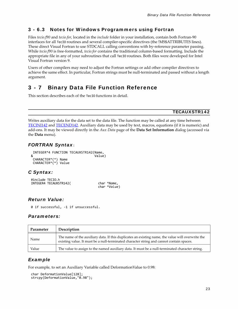
TECAUXSTR142
Writes auxiliary data for the data set to the data file. The function may be called at any time between TECINI142 and TECEND142. Auxiliary data may be used by text, macros, equations (if it is numeric) and add-ons. It may be viewed directly in the Aux Data page of the Data Set Information dialog (accessed via the Data menu).
FORTRAN Syntax:
INTEGER*4 FUNCTION TECAUXSTR142(Name,& Value) CHARACTER*(*) Name CHARACTER*(*) Value
C Syntax:#include TECIO.hINTEGER4 TECAUXSTR142( char *Name,
char *Value)
Return Value:0 if successful, -1 if unsuccessful.
Parameters:
ExampleFor example, to set an Auxiliary Variable called DeformationValue to 0.98:
char DeformationValue[128];strcpy(DeformationValue,"0.98");
Parameter Description
Name The name of the auxiliary data. If this duplicates an existing name, the value will overwrite the existing value. It must be a null-terminated character string and cannot contain spaces.
Value The value to assign to the named auxiliary data. It must be a null-terminated character string.

24
TECAUXSTR142("DeformationValue", DeformationValue);
When the data file is loaded into Tecplot, “Deformation Value” will appear on the Aux Page of the Data Set Information dialog when “for Data Set” is selected in Show Auxiliary Data menu.
TECDAT142
Writes an array of data to the data file. Data should not be passed for variables that have been indicated as passive or shared (via TECZNE142).
TECDAT142 allows you to write your data in piecemeal fashion in case it is not contained in one contiguous block in your program or is not available all at once. TECDAT142 must be called enough times to ensure that the correct number of values is written for each zone and that the aggregate order for the data is correct.
In the above summary, NumVars is based on the number of variable names supplied in a previous call to TECINI142.
FORTRAN Syntax:
INTEGER*4 FUNCTION TECDAT142(N,& Data,& IsDouble) INTEGER*4 N REAL or DOUBLE PRECISION Data(1) INTEGER*4 IsDouble
C Syntax:#include TECIO.hINTEGER4 TECDAT142( INTEGER4 *N,
void *Data,INTEGER4 *IsDouble);
Return Value:0 if successful, -1 if unsuccessful.

25
Binary Data File Function Reference
Parameters:
Data ArrangementThe following table describes the order the data must be supplied given different zone types. IsBlock and VarLocation are parameters supplied to TECZNE142. The value of IsBlock should always be 1, since binary data must be written in block format:
ExampleRefer to the following examples in Section 3 - 9 “Examples” for examples using TECDAT142:
• Section 3 - 9.1 “Face Neighbors”• Section 3 - 9.2 “Polygonal Example”
Parameter Description
N Pointer to an integer value specifying number of values to write.
Data Array of single or double precision data values. Refer to Table 3 - 1 for a description of how to arrange your data.
IsDouble Pointer to the integer flag stating whether the array Data is single (0) or double (1) precision.
Zone Type
Var. Location IsBlock Number of Values
Order
Ordered Nodal 1
IMax*JMax*KMax*NumVars
I varies fastest, then J, then K, then Vars. That is, the numbers should be supplied in the following order: for (Var=1;Var<=NumVars;Var++) for (K=1;K<=KMax;K++) for (J=1;J<=JMax;J++) for (I=1;I<=IMax;I++) Data[I, J, K, Var] = value;
Ordered Cell Centered 1
(IMax-1)*(JMax-1)*(KMax-1)*NumVars
I varies fastest, then J, then K, then Vars. That is, the numbers should be supplied in the following order: for (Var=1;Var<=NumVars;Var++) for (K=1;K<=(KMax-1);K++) for (J=1;J<=(JMax-1);J++) for (I=1;I<=(IMax-1);I++) Data[I, J, K, Var] = value;
Finite element Nodal 1
IMax (i.e. NumNodes) * NumVars
N varies fastest, then Vars. That is, the numbers should be supplied in the following order: for (Var=1;Var<=NumVars;Var++) for (N=1;N<=NumNodes;N++) Data[N, Var] = value;
Finite element Cell Centered 1
JMax (i.e. NumElements) * NumVars
E varies fastest, then Var. That is, the numbers should be supplied in the following order: for (Var=1;Var<=NumVars;Var++) for (E=1;E<=NumElements;E++) Data[E, Var] = value;
Table 3 - 1: Data Arrangement

26
• Section 3 - 9.3 “Multiple Polyhedral Zones”• Section 3 - 9.4 “Multiple Polygonal Zones”• Section 3 - 9.5 “Polyhedral Example”• Section 3 - 9.6 “IJ-ordered zone”
TECEND142
Must be called to close the current data file. There must be one call to TECEND142 for each TECINI142.
FORTRAN Syntax:INTEGER*4 FUNCTION TECEND142()
C Syntax:#include TECIO.hINTEGER4 TECEND142();
Return Value:0 if successful, -1 if unsuccessful.
Parameters:None.
TECFACE142
Writes face connections for the current zone to the file. Face Neighbor Connections are used for ordered or cell-based finite element zones to specify connections that are not explicitly defined by the connectivity list or ordered zone structure. You many use face neighbors to specify connections between zones (global connections) or connections within zones (local connections). Face neighbor connections are used by Tecplot when deriving variables or drawing contour lines. Specifying face neighbors, typically leads to smoother connections. NOTE: face neighbors have expensive performance implications. Use face neighbors only to manually specify connections that are not defined via the connectivity list.
This function must be called after TECNOD142 or TECNODE142, and may only be called if a non-zero value of NumFaceConnections was used in the previous call to TECZNE142.
FORTRAN Syntax:INTEGER*4 FUNCTION TECFACE142(FaceConnections)INTEGER*4 FACECONNECTIONS(*)
C Syntax:#include TECIO.hINTEGER4 TECFACE142(INTEGER4 *FaceConnections);
Return Value:0 if successful, -1 if unsuccessful.

27
Binary Data File Function Reference
Parameters:
Where:
cz = cell in current zone
fz = face of cell in current zone
oz = face obscuration flag (only applies to one-to-many):
0 = face partially obscured
1 = face entirely obscured
nz = number of cell or zone/cell associations (only applies to one-to-many)
ZZ = remote Zone
CZ = cell in remote zone
cz,fz combinations must be unique. Additionally, Tecplot 360 assumes that with the one-to-one face neighbor modes a supplied cell face is entirely obscured by its neighbor. With one-to-many, the obscuration flag must be supplied. Faces that are not supplied with neighbors are run through Tecplot 360’s auto face neighbor generator (FE only).
Parameter Description
FaceConnections
The array that specifies the face connections. The array must have L values, where L is the sum of the number of values for each face neighbor connection in the data file. The number of values in a face neighbor connection is dependent upon the FaceNeighborMode parameter (set via TECZNE142) and is described in the following table.
FaceNeighbor Mode Number of values
Data
LocalOneToOne 3 cz1,fz,cz2
LocalOneToMany nz+4 cz1,fz,oz,nz,cz2,cz3,...,czn
GlobalOneToOne 4 cz, fz, ZZ, CZ
GlobalOneToMany 2*nz+4 cz, fz, oz, nz, ZZ1, CZ1, ZZ2, CZ2, ...,ZZn, CZn

28
The face numbers for cells in the various zone types are defined in Figure 3-1.
Figure 3-1. A: Example of node and face neighbors for an FE-brick cell or IJK-ordered cell. B: Example of node and face numbering for an IJ-ordered/ FE-quadrilateral cell. C: Example of tetrahedron face neighbors.
ExampleRefer to Section 3 - 9.1 “Face Neighbors” for an example of working with face neighbors. In this example, face neighbors are used to prevent an Edge line from being drawn between the two zones.
TECFIL142
Switch output context to a different file. Each time TECINI142 is called the file context is switched to a different file. This allows you to write multiple data files at the same time. When working with multiple files, be sure to call TECFIL142 each time you wish to write to a file. This will ensure your data is written to the appropriate file.
FORTRAN Syntax: INTEGER*4 FUNCTION TECFIL142(F)INTEGER*4 F
C Syntax:#include TECIO.hINTEGER4 TECFIL142(INTEGER4 *F);
Return Value:0 if successful, -1 if unsuccessful.
A B C

29
Binary Data File Function Reference
Parameters:
ExamplesRefer to Section 3 - 9.7 “Switching Between Two Files” for a simple example of working with TECFIL142.
TECFOREIGN142
Optional function that sets the byte ordering request for subsequent calls to TECINI142. The byte ordering request will remain in effect until the next call to this function. This has no effect on files already opened via TECINI142. Use this function to reverse the byte ordering from the format native to your operating system. For example, this is useful if you are creating a file on an SGI machine to be used on a Windows or Intel-based Linux machine. If the function call is omitted, native byte ordering will be used.
FORTRAN Syntax: INTEGER*4 FUNCTION TECFOREIGN142(DoForeignByteOrder)INTEGER*4 DoForeignByteOrder
C Syntax:#include TECIO.hINTEGER4 TECFOREIGN142(INTEGER4 *DoForeignByteOrder);
Return Value:0 if successful, -1 if unsuccessful.
Parameters:
TECGEO142
Adds a geometry object to the file (e.g. a circle or a square). NOTE: you cannot set unused parameters to NULL. You must use dummy values for unused parameters.
FORTRAN Syntax:
INTEGER*4 FUNCTION TECGEO142( XOrThetaPos,& YOrRPos,& ZPos,& PosCoordMode,& AttachToZone,
Parameter Description
F Pointer to integer specifying file number to switch to. A value of 1 indicates a switch to the file opened by the first call to TECINI142.
Parameter Description
DoForeignByteOrder
Pointer to boolean value indicating if future files created by TECINI142 should be written out in foreign byte order. 0 indicates native byte order. 1 indicates foreign byte order.

30
& Zone,& Color,& FillColor,& IsFilled,& GeomType,& LinePattern,& PatternLength,& LineThicknessness,& NumEllipsePts,& ArrowheadStyle,& ArrowheadAttachment,& ArrowheadSize,& ArrowheadAngle,& Scope,& Clipping,& NumSegments,& NumSegPts,& XOrThetaGeomData,& YOrRGeomData,& ZGeomData,& MFC) DOUBLE PRECISION XOrThetaPos DOUBLE PRECISION YOrRPos DOUBLE PRECISION ZPos INTEGER*4 PosCoordMode INTEGER*4 AttachToZone INTEGER*4 Zone INTEGER*4 Color INTEGER*4 FillColor INTEGER*4 IsFilled INTEGER*4 GeomType INTEGER*4 LinePattern DOUBLE PRECISION PatternLength DOUBLE PRECISION LineThicknessness INTEGER*4 NumEllipsePts INTEGER*4 ArrowheadStyle INTEGER*4 ArrowheadAttachment DOUBLE PRECISION ArrowheadSize DOUBLE PRECISION ArrowheadAngle INTEGER*4 Scope INTEGER*4 Clipping INTEGER*4 NumSegments INTEGER*4 NumSegPts REAL*4 XOrThetaGeomData REAL*4 YOrRGeomData REAL*4 ZGeomData CHARACTER*(*) MFC
C Syntax:#include TECIO.hINTEGER4 TECGEO142(double *XOrThetaPos,double *YOrRPos,double *ZPos,INTEGER4 *PosCoordMode,INTEGER4 *AttachToZone,INTEGER4 *Zone,INTEGER4 *Color,INTEGER4 *FillColor,INTEGER4 *IsFilled,INTEGER4 *GeomType,INTEGER4 *LinePattern,double *PatternLength,double *LineThicknessness,INTEGER4 *NumEllipsePts,INTEGER4 *ArrowheadStyle,INTEGER4 *ArrowheadAttachment,double *ArrowheadSize,double *ArrowheadAngle,INTEGER4 *Scope,INTEGER4 *Clipping,

31
Binary Data File Function Reference
INTEGER4 *NumSegments,INTEGER4 *NumSegPts,float *XOrThetaGeomData,float *YOrRGeomData,float *ZGeomData,char *MFC
Return Value:0 if successful, -1 if unsuccessful.
32
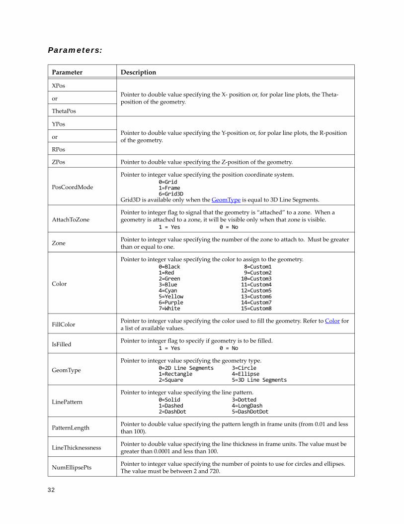
Parameters:
Parameter Description
XPos Pointer to double value specifying the X- position or, for polar line plots, the Theta-position of the geometry.or
ThetaPos
YPosPointer to double value specifying the Y-position or, for polar line plots, the R-position of the geometry.or
RPos
ZPos Pointer to double value specifying the Z-position of the geometry.
PosCoordMode
Pointer to integer value specifying the position coordinate system. 0=Grid1=Frame6=Grid3D
Grid3D is available only when the GeomType is equal to 3D Line Segments.
AttachToZone Pointer to integer flag to signal that the geometry is “attached” to a zone. When a geometry is attached to a zone, it will be visible only when that zone is visible.
1 = Yes 0 = No
Zone Pointer to integer value specifying the number of the zone to attach to. Must be greater than or equal to one.
Color
Pointer to integer value specifying the color to assign to the geometry. 0=Black 8=Custom11=Red 9=Custom22=Green 10=Custom33=Blue 11=Custom44=Cyan 12=Custom55=Yellow 13=Custom66=Purple 14=Custom77=White 15=Custom8
FillColor Pointer to integer value specifying the color used to fill the geometry. Refer to Color for a list of available values.
IsFilled Pointer to integer flag to specify if geometry is to be filled.1 = Yes 0 = No
GeomType Pointer to integer value specifying the geometry type.
0=2D Line Segments 3=Circle1=Rectangle 4=Ellipse2=Square 5=3D Line Segments
LinePattern Pointer to integer value specifying the line pattern.
0=Solid 3=Dotted1=Dashed 4=LongDash2=DashDot 5=DashDotDot
PatternLength Pointer to double value specifying the pattern length in frame units (from 0.01 and less than 100).
LineThicknessness Pointer to double value specifying the line thickness in frame units. The value must be greater than 0.0001 and less than 100.
NumEllipsePts Pointer to integer value specifying the number of points to use for circles and ellipses. The value must be between 2 and 720.

33
Binary Data File Function Reference
Origin positionsThe origin (XOrThetaPos, YOrRPos, ZPos) of each geometry type is listed below:
• SQUARE - lower left corner at XOrThetaPos, YOrRPos.• RECTANGLE - lower left corner at XOrThetaPos, YOrRPos.• CIRCLE - centered at XOrThetaPos, YOrRPos.• ELLIPSE - centered at XOrThetaPos, YOrRPos.• LINE - anchored at XOrThetaPos, YOrRPos.• LINE3D - anchored at XOrThetaPos, YOrRPos, ZPos.
Data ValuesThe origin (XOrThetaGeomData, YOrRGeomData, ZGeomData) of each geometry type is listed below:
• SQUARE - set XOrThetaGeomData equal to the desired length.• RECTANGLE - set XOrThetaGeomData equal to the desired width and YOrThetaGeomData equal to
the desired height.• CIRCLE - set XOrThetaGeomData equal to the desired radius.
ArrowheadStyle Pointer to integer value specifying the arrowhead style.
0=Plain 2=Hollow1=Filled
ArrowheadAttachment
Pointer to integer value specifying where to attach arrowheads. 0=None 2=End1=Beginning 3=Both
ArrowheadSize Pointer to double value specifying the arrowhead size in frame units (from 0 to 100).
ArrowheadAngle Pointer to double value specifying the arrowhead angle in degrees.
Scope
Pointer to integer value specifying the scope with respect to frames. A local scope places the object in the active frame. A global scope places the object in all frames that contain the active frame’s data set.
0=Global 1=Local.
Clipping Specifies whether to clip the geometry (that is, only plot the geometry within) to the viewport or the frame.
0=ClipToViewport 1=ClipToFrame.
NumSegments Pointer to integer value specifying the number of polyline segments.
NumSegPts Array of integer values specifying the number of points in each of the NumSegments segments.
XGeomData
Array of floating-point values specifying the X-, Y- and Z-coordinates. Refer to “Data Values” on page 33 for information regarding the values required for each GeomType.
ThetaGeomData
YGeomData
RGeomData
ZGeomData
MFC Macro function command. Must be null terminated.
Parameter Description

34
• ELLIPSE - set XOrThetaGeomData equal to the desired width along the x-axis and YOrThetaGeomData equal to the desired width along the y-axis.
• LINE - specify the coordinate positions for the data points in each line segment with XOrThetaGeomData and YOrRGeomData.
• LINE3D - specify the coordinate positions for the data points in each line segment with XOrThetaGeomData, YOrRGeomData and ZGeomData.
TECINI142
Initializes the process of writing a binary data file. Either this function or TECINI142 must be called first before any other TecIO calls are made (except TECFOREIGN142). You may write to multiple files by calling TECINI142 more than once. Each time TECINI142 is called, a new file is opened. Use TECFIL142 to switch between files. For each call to TECINI, there must be a corresponding call to TECEND142.
FORTRAN Syntax: INTEGER*4 FUNCTION TECINI142( Title,& Variables,& FName,& ScratchDir,& FileFormat,& FileType,& Debug,& VIsDouble)CHARACTER*(*) TitleCHARACTER*(*) VariablesCHARACTER*(*) ScratchDirCHARACTER*(*) FNameINTEGER*4 FileFormatINTEGER*4 FileTypeINTEGER*4 DebugINTEGER*4 VIsDouble
C Syntax:#include TECIO.hINTEGER4 TECINI142(char *Title,
char *Variables,char *FName,char*ScratchDir,INTEGER4*FileFormat,INTEGER4*FileType,INTEGER4*DebugINTEGER4*VIsDouble);
Return Value:0 if successful, -1 if unsuccessful.

35
Binary Data File Function Reference
Parameters:
ExamplesEach example in Section 3 - 9 “Examples” calls TECINI142 at least once. Refer to this section for details.
TECLAB142
Adds custom labels to the data file. Custom Labels can be used for axis labels, legend text, and tick mark labels. The first custom label string corresponds to a value of one on the axis, the next to a value of two, the next to a value of three, and so forth. You must have at least one zone in your data set.
A custom label set is added to your file each time you call TECLAB142. You may have up to sixty labels in a set and up to ten sets in a file. Each label must be surrounded by double-quotes, e.g. “Mon” “Tues” “Wed”, etc. The \n escape sequence may be used to indicate a line break.
Custom labels are assigned to an object via the Tecplot interface. Refer to Section 17 - 8 “Axis Title Options” in the User’s Manual for details.
FORTRAN Syntax:INTEGER*4 FUNCTION TECLAB142(Labels)CHARACTER*(*) Labels
C Syntax:#include TECIO.hINTEGER4 TECLAB142(char *Labels);
Return Value:0 if successful, -1 if unsuccessful.
Parameter Description
Title Title of the data set. Must be null terminated.
Variables List of variable names. If a comma appears in the string it will be used as the separator between variable names, otherwise a space is used. Must be null terminated.
FName Name of the file to create. Must be null terminated.
ScratchDir Name of the directory to put the scratch file. Must be null terminated.
FileFormat Specifies the file format to be used.0=Tecplot binary (.plt) 1=Tecplot subzone loadable (.szplt)
FileType Specify whether the file is a full data file (containing both grid and solution data), a grid file or a solution file.
0=Full 1=Grid 2=Solution
Debug Pointer to the integer flag for debugging. Set to 0 for no debugging or 1 to debug. When set to 1, the debug messages will be sent to the standard output (stdout).
VIsDouble Pointer to the integer flag for specifying whether field data generated in future calls to TECDAT142 are to be written in single or double precision.
0=Single 1=Double

36
Parameters:
ExamplesTo add the days of the week to your data file, to be displayed along the x-axis:
char Labels[60] = "\"Mon\", \"Tues\",\"Wed\",\"Thurs\", \”Fri\”";TECLAB142(&Labels[0]);
TECNOD142
Writes an array of node data to the binary data file. This is the connectivity list for cell-based finite element zones (line segment, triangle, quadrilateral, brick, and tetrahedral zones). The connectivity list for face-based finite element zones (polygonal and polyhedral) is specified via TECPOLY142.
See also TECNODE142, which allows you to provide connectivity information in arbitrarily-sized chunks rather than requiring it all at once.
FORTRAN Syntax:INTEGER*4 FUNCTION TECNOD142(NData)INTEGER*4 NData (T, M)
C Syntax:#include TECIO.hINTEGER4 TECNOD142(INTEGER4 *NData);
Return Value:0 if successful, -1 if unsuccessful.
Parameters:
Examples:Refer to Section 3 - 9.1 “Face Neighbors” for examples using TECNOD142.
Parameter Description
Labels Character string of custom labels. Each label must be surrounded by double-quotes. Separate labels by a comma or space. You may have up to sixty labels in each call to TECLAB142.
Parameter Description
NData
Array of integers listing the nodes for each element. This is the connectivity list, dimensioned (T, M) (T moving fastest), where M is the number of elements in the zone and T is set according to the following list:
2=Line Segment 4=Tetrahedral3=Triangle 8=Brick4=Quadrilateral

37
Binary Data File Function Reference
TECNODE142
Writes a chunk of node data to the binary data file. This is the connectivity list for cell-based finite element zones (line segment, triangle, quadrilateral, brick, and tetrahedral zones). The connectivity list for face-based finite element zones (polygonal and polyhedral) is specified via TECPOLY142.
This function is similar to TECNOD142 but does not require that the entire connectivity list be provided at once. Rather, you may call TECNODE142 as many times as you like, providing connectivity information for as many elements as you like each time, so long as you eventually provide connectivity information for all elements in the zone.
FORTRAN Syntax:INTEGER*4 FUNCTION TECNODE142(N, NData)INTEGER*4 NINTEGER*4 NData (T, M)
C Syntax:#include TECIO.hINTEGER4 TECNODE142(INTEGER4 *N, INTEGER4 *NData);
Return Value:0 if successful, -1 if unsuccessful.
Parameters:
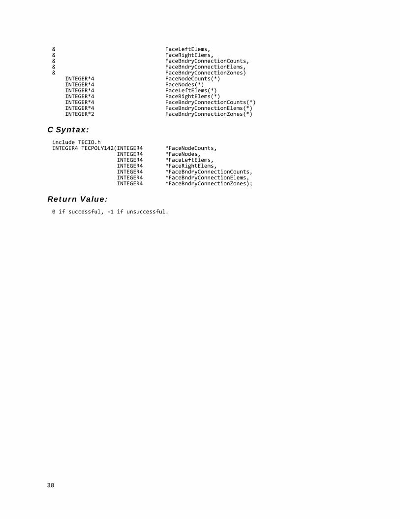
TECPOLY142
Writes the face map for polygonal and polyhedral zones to the data file. All numbering schemes are one-based. The first node is Node 1, the first face is Face 1, and so forth. Refer to Section 3 - 8 “Defining Polyhedral and Polygonal Data” on page 52 for additional information.
The TECPOLY142 function requires that all face map data, both face nodes and boundary connections, be provided with a single call. For most applications, we recommend you use TECPOLYFACE142 and TECPOLYBCONN142 instead, as these do not have this requirement and can be used when the face map data is not available all at once or will not fit into memory.
Avoid creating concave objects (or bad meshes), as they will not look good when plotted.
FORTRAN syntax: INTEGER*4 FUNCTION TECPOLY142(& FaceNodeCounts,& FaceNodes,
Parameter Description
N Handle to an integer indicating the number of values to write.
NData
Array of integers listing the nodes for each element. This is the connectivity list, dimensioned (T, N) (T moving fastest), where N is the number of elements provided in this call to TECNODE142 and T is set according to the following list:
2=Line Segment 4=Tetrahedral3=Triangle 8=Brick4=Quadrilateral
38
& FaceLeftElems,& FaceRightElems,& FaceBndryConnectionCounts,& FaceBndryConnectionElems,& FaceBndryConnectionZones) INTEGER*4 FaceNodeCounts(*) INTEGER*4 FaceNodes(*) INTEGER*4 FaceLeftElems(*) INTEGER*4 FaceRightElems(*) INTEGER*4 FaceBndryConnectionCounts(*) INTEGER*4 FaceBndryConnectionElems(*) INTEGER*2 FaceBndryConnectionZones(*)
C Syntax:include TECIO.hINTEGER4 TECPOLY142(INTEGER4 *FaceNodeCounts, INTEGER4 *FaceNodes, INTEGER4 *FaceLeftElems, INTEGER4 *FaceRightElems, INTEGER4 *FaceBndryConnectionCounts, INTEGER4 *FaceBndryConnectionElems, INTEGER4 *FaceBndryConnectionZones);
Return Value:0 if successful, -1 if unsuccessful.
39
Binary Data File Function Reference
Parameters:
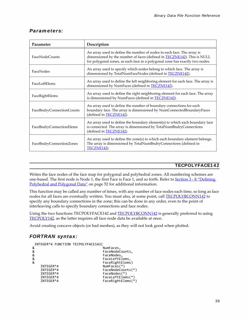
TECPOLYFACE142
Writes the face nodes of the face map for polygonal and polyhedral zones. All numbering schemes are one-based. The first node is Node 1, the first Face is Face 1, and so forth. Refer to Section 3 - 8 “Defining Polyhedral and Polygonal Data” on page 52 for additional information.
This function may be called any number of times, with any number of face nodes each time, so long as face nodes for all faces are eventually written. You must also, at some point, call TECPOLYBCONN142 to specify any boundary connections in the zone; this can be done in any order, even to the point of interleaving calls to specify boundary connections and face nodes.
Using the two functions TECPOLYFACE142 and TECPOLYBCONN142 is generally preferred to using TECPOLY142, as the latter requires all face node data be available at once.
Avoid creating concave objects (or bad meshes), as they will not look good when plotted.
FORTRAN syntax: INTEGER*4 FUNCTION TECPOLYFACE142(& NumFaces,& FaceNodeCounts,& FaceNodes,& FaceLeftElems,& FaceRightElems) INTEGER*4 NumFaces(*) INTEGER*4 FaceNodeCounts(*) INTEGER*4 FaceNodes(*) INTEGER*4 FaceLeftElems(*) INTEGER*4 FaceRightElems(*)
Parameter Description
FaceNodeCounts An array used to define the number of nodes in each face. The array is dimensioned by the number of faces (defined in TECZNE142). This is NULL for polygonal zones, as each face in a polygonal zone has exactly two nodes.
FaceNodes An array used to specify which nodes belong to which face. The array is dimensioned by TotalNumFaceNodes (defined in TECZNE142).
FaceLeftElems An array used to define the left neighboring element for each face. The array is dimensioned by NumFaces (defined in TECZNE142).
FaceRightElems An array used to define the right neighboring element for each face. The array is dimensioned by NumFaces (defined in TECZNE142).
FaceBndryConnectionCountsAn array used to define the number of boundary connections for each boundary face. The array is dimensioned by NumConnectedBoundaryFaces (defined in TECZNE142).
FaceBndryConnectionElemsAn array used to define the boundary element(s) to which each boundary face is connected. The array is dimensioned by TotalNumBndryConnections (defined in TECZNE142).
FaceBndryConnectionZones An array used to define the zone(s) to which each boundary element belongs. The array is dimensioned by TotalNumBndryConnections (defined in TECZNE142).

40
C Syntax:include TECIO.hINTEGER4 TECPOLYFACE142(INTEGER4 *NumFaces, INTEGER4 *FaceNodeCounts, INTEGER4 *FaceNodes, INTEGER4 *FaceLeftElems, INTEGER4 *FaceRightElems);
Return Value:0 if successful; -1 if unsuccessful.
Parameters:
Examples:Refer to the following sections for examples using TECPOLYFACE142:
• 3 - 9.2 “Polygonal Example”• 3 - 9.3 “Multiple Polyhedral Zones”• 3 - 9.4 “Multiple Polygonal Zones”• 3 - 9.5 “Polyhedral Example”
TECPOLYBCONN142
Writes the boundary connections of the face map for polygonal and polyhedral zones. Boundary faces are faces that either have more than one neighboring cell on a side or have at least one neighboring cell in another zone. (Refer to Section 3 - 8.1 “Boundary Faces and Boundary Connections” on page 52 for a simple example.)
All numbering schemes are one-based. The first node is Node 1, the first face is Face 1, and so forth. Refer to Section 3 - 8 “Defining Polyhedral and Polygonal Data” on page 52 for additional information.
This function may be called any number of times, with any number boundary connections each time, so long as boundary connections for all faces are eventually written. You must also, at some point, call TECPOLYFACE142 at least once to specify the face nodes. This can be done in any order, even to the point of interleaving calls to specify boundary connections and face nodes.
Parameter Description
NumFacesThe number of faces being defined in this call. TECPOLYFACE142 may be called any number of times with any number of faces in each call, so long as all faces in the zone are eventually defined.
FaceNodeCountsAn array used to define the number of nodes in each face. The array is dimensioned by NumFaces. This is NULL for polygonal zones, as each face in a polygonal zone is already known to have exactly two nodes.
FaceNodes An array used to specify the nodes belonging to each face. The array is dimensioned by the sum of the FaceNodeCounts array for polyhedral zones or, for polygonal zones, twice NumFaces.
FaceLeftElems An array used to define the left neighboring element for each face. The array is dimensioned by NumFaces.
FaceRightElems An array used to define the right neighboring element for each face. The array is dimensioned by NumFaces.

41
Binary Data File Function Reference
Using the two functions TECPOLYFACE142 and TECPOLYBCONN142 is generally preferred to using TECPOLY142, as the latter requires that all face map data (including boundary connections) be available at once.
Avoid creating concave objects (or bad meshes), as they will not look good when plotted.
FORTRAN syntax: INTEGER*4 FUNCTION TECPOLYBCONN142(& NumBndryFaces,& FaceBndryConnectionCounts,& FaceBndryConnectionElems,& FaceBndryConnectionZones) INTEGER*4 NumBndryFaces(*) INTEGER*4 FaceBndryConnectionCounts(*) INTEGER*4 FaceBndryConnectionElems(*) INTEGER*2 FaceBndryConnectionZones(*)
C Syntax:#include TECIO.hINTEGER4 TECPOLYBCONN142(INTEGER4 *NumBndryFaces, INTEGER4 *FaceBndryConnectionCounts, INTEGER4 *FaceBndryConnectionElems, INTEGER4 *FaceBndryConnectionZones);
Return Value:0 if successful, -1 if unsuccessful.
Parameters:
Examples:Refer to the following sections for examples using TECPOLYBCONN142:
• 3 - 9.2 “Polygonal Example”• 3 - 9.3 “Multiple Polyhedral Zones”• 3 - 9.4 “Multiple Polygonal Zones”• 3 - 9.5 “Polyhedral Example”
Parameter Description
NumBndryFaces
The number of boundary faces being defined in this call. Each call to TECPOLYBCONN142 may define any number of boundary faces, so long as all boundary faces (i.e., NumConnectedBoundaryFaces in TECZNE142) are eventually defined.
FaceBndryConnectionCounts An array used to define the number of boundary connections for each boundary face. The array is dimensioned by NumBndryFaces.
FaceBndryConnectionElems An array used to define the boundary element(s) to which each boundary face is connected.
FaceBndryConnectionZones An array used to define the zone(s) to which each boundary element belongs.

42
TECTXT142
Adds a text box to the file.
FORTRAN Syntax: INTEGER*4 FUNCTION TECTXT142( XOrThetaPos,& YOrRPos,& ZOrUnusedPos,& PosCoordMode,&& AttachToZone,& Zone,& Font,& FontHeightUnits,& FontHeight,& BoxType,& BoxMargin,& BoxLineThickness,& BoxColor,& BoxFillColor,& Angle,& Anchor,& LineSpacing,& TextColor,& Scope,& Clipping,& Text,& MFC) DOUBLE PRECISION XOrThetaPos DOUBLE PRECISION YOrRPos DOUBLE PRECISION ZOrUnusedPos INTEGER*4 PosCoordMode INTEGER*4 AttachToZone INTEGER*4 Zone INTEGER*4 Font INTEGER*4 FontHeightUnits DOUBLE PRECISION FontHeight INTEGER*4 BoxType DOUBLE PRECISION BoxMargin DOUBLE PRECISION BoxLineThickness INTEGER*4 BoxColor INTEGER*4 BoxFillColor DOUBLE PRECISION Angle INTEGER*4 Anchor DOUBLE PRECISION LineSpacing INTEGER*4 TextColor INTEGER*4 Scope INTEGER*4 Clipping CHARACTER*(*) Text CHARACTER*(*) MFC
C Syntax:#include TECIO.hINTEGER4 TECTXT142( double *XOrThetaPos,
double *YOrRPos,double *ZOrUnusedPos,INTEGER4*PosCoordMode,INTEGER4*AttachToZone,INTEGER4*Zone,INTEGER4*Font,INTEGER4*FontHeightUnits,double*FontHeight,INTEGER4*BoxType,double*BoxMargin,double*BoxLineThickness,INTEGER4*BoxColor,INTEGER4*BoxFillColor,double*Angle,

43
Binary Data File Function Reference
INTEGER4*Anchor,double*LineSpacing,INTEGER4*TextColor,INTEGER4*Scope,INTEGER4*Clipping,char*Text,char*MFC)
Return Value: 0 if successful, -1 if unsuccessful.

44
Parameters:
Parameter Description
XOrThetaPos Pointer to double value specifying the X-position or Theta-position (polar plots only) of the text.
YOrRPos Pointer to double value specifying the Y-position or R-position (polar plots only) of the text.
ZOrUnusedPos Pointer to double value specifying the Z-position of the text.
PosCoordMode
Pointer to integer value specifying the position coordinate system. 0=Grid1=Frame6=Grid3D
If you use Grid3D, the plot type must be set to 3D Cartesian to view your text box.
AttachToZone Pointer to integer flag to signal that the text is “attached” to a zone.
Zone Pointer to integer value specifying the zone number to attach to.
Font
Pointer to integer value specifying the font. 0=Helvetica 6=Times Italic1=Helvetica Bold 7=Times Bold2=Greek 8=Times Italic Bold3=Math 9=Courier4=User-Defined 10=Courier Bold5=Times
FontHeightUnits Pointer to integer value specifying the font height units.
0=Grid 2=Point1=Frame
FontHeight Pointer to double value specifying the font height. If PosCoordMode is set to FRAME, the value range is zero to 100.
BoxType Pointer to integer value specifying the box type.
0=None 2=Hollow1=Filled
BoxMargin Pointer to double value specifying the box margin (in frame units ranging from 0 to 100).
BoxLineThickness Pointer to double value specifying the box line thickness (in frame units ranging from 0.0001 to 100).
BoxColor
Pointer to integer value specifying the color to assign to the box. 0=Black 8=Custom11=Red 9=Custom22=Green 10=Custom33=Blue 11=Custom44=Cyan 12=Custom55=Yellow 13=Custom66=Purple 14=Custom77=White 15=Custom8
BoxFillColor Pointer to integer value specifying the fill color to assign to the box. (See BoxColor)
Angle Pointer to double value specifying the text angle in degrees.
Anchor
Pointer to integer value specifying where to anchor the text. 0=Left 5=MidRight1=Center 6=HeadLeft2=Right 7=HeadCenter3=MidLeft 8=HeadRight4=MidCenter
45
Binary Data File Function Reference
ExamplesRefer to Section 3 - 9.8 “Text Example” for an example of working with TECTXT142.
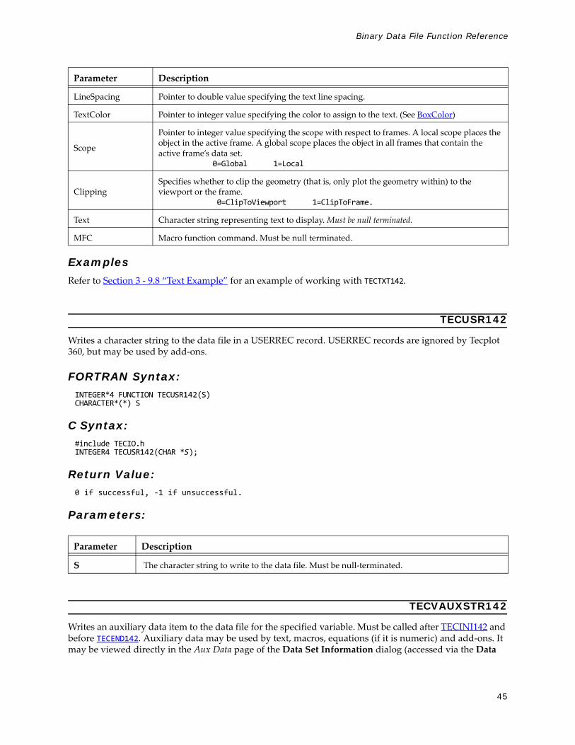
TECUSR142
Writes a character string to the data file in a USERREC record. USERREC records are ignored by Tecplot 360, but may be used by add-ons.
FORTRAN Syntax:INTEGER*4 FUNCTION TECUSR142(S)CHARACTER*(*) S
C Syntax:#include TECIO.hINTEGER4 TECUSR142(CHAR *S);
Return Value:0 if successful, -1 if unsuccessful.
Parameters:
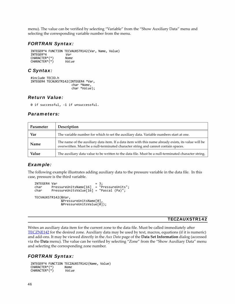
TECVAUXSTR142
Writes an auxiliary data item to the data file for the specified variable. Must be called after TECINI142 and before TECEND142. Auxiliary data may be used by text, macros, equations (if it is numeric) and add-ons. It may be viewed directly in the Aux Data page of the Data Set Information dialog (accessed via the Data
LineSpacing Pointer to double value specifying the text line spacing.
TextColor Pointer to integer value specifying the color to assign to the text. (See BoxColor)
Scope
Pointer to integer value specifying the scope with respect to frames. A local scope places the object in the active frame. A global scope places the object in all frames that contain the active frame’s data set.
0=Global 1=Local
Clipping Specifies whether to clip the geometry (that is, only plot the geometry within) to the viewport or the frame.
0=ClipToViewport 1=ClipToFrame.
Text Character string representing text to display. Must be null terminated.
MFC Macro function command. Must be null terminated.
Parameter Description
S The character string to write to the data file. Must be null-terminated.
Parameter Description
46
menu). The value can be verified by selecting “Variable” from the “Show Auxiliary Data” menu and selecting the corresponding variable number from the menu.
FORTRAN Syntax: INTEGER*4 FUNCTION TECVAUXSTR142(Var, Name, Value)INTEGER*4 VarCHARACTER*(*) NameCHARACTER*(*) Value
C Syntax:#include TECIO.hINTEGER4 TECAUXSTR142(INTEGER4 *Var, char *Name, char *Value);
Return Value:0 if successful, -1 if unsuccessful.
Parameters:
Example:The following example illustrates adding auxiliary data to the pressure variable in the data file. In this case, pressure is the third variable.
INTEGER4 Var = 3; char PressureUnitsName[16] = "PressureUnits"; char PressureUnitsValue[16] = "Pascal (Pa)"; TECVAUXSTR142(&Var, &PressureUnitsName[0], &PressureUnitsValue[0]);
TECZAUXSTR142
Writes an auxiliary data item for the current zone to the data file. Must be called immediately after TECZNE142 for the desired zone. Auxiliary data may be used by text, macros, equations (if it is numeric) and add-ons. It may be viewed directly in the Aux Data page of the Data Set Information dialog (accessed via the Data menu). The value can be verified by selecting “Zone” from the “Show Auxiliary Data” menu and selecting the corresponding zone number.
FORTRAN Syntax:INTEGER*4 FUNCTION TECZAUXSTR142(Name, Value)CHARACTER*(*) NameCHARACTER*(*) Value
Parameter Description
Var The variable number for which to set the auxiliary data. Variable numbers start at one.
Name The name of the auxiliary data item. If a data item with this name already exists, its value will be overwritten. Must be a null-terminated character string and cannot contain spaces.
Value The auxiliary data value to be written to the data file. Must be a null-terminated character string.

47
Binary Data File Function Reference
C Syntax:#include TECIO.hINTEGER4 TECZAUXSTR142(char *Name, char *Value);
Return Value:0 if successful, -1 if unsuccessful.
Parameters:
Example:The following example code adds auxiliary data to the zone. NOTE: TECZAUXSTR142 must be called immediately after TECZNE142 for the desired zone.
char CreatedByName[16] = "CreatedBy";char CreatedByValue[16] = "My Company";
TECZAUXSTR142(&CreatedByName[0], &CreatedByValue[0]);
TECZNE142
Writes header information about the next zone to be added to the data file. After TECZNE142 is called, you must call TECDAT142 one or more times. If the zone is a finite element zone, call TECNOD142/TECNODE142 (cell-based zones) or TECPOLY142/TECPOLYFACE142/TECPOLYBCONN142 (face-based zones) after calling TECDAT142.
FORTRAN Syntax: INTEGER*4 FUNCTION TECZNE142(ZoneTitle,& ZoneType,& IMxOrNumPts,& JMxOrNumElements,& KMxOrNumFaces,& ICellMax,& JCellMax,& KCellMax,& SolutionTime,& StrandID,& ParentZone,& IsBlock,
Parameter Description
Name The name of the auxiliary data item. If a data item with this name already exists, its value will be overwritten. Must be a null-terminated character string and cannot contain spaces.
Value The auxiliary data value to be written to the data file. Must be a null-terminated character string.
When specifiying your ZoneType, please note that some features in Tecplot 360 are limited by zone type. For example, iso-surfaces and slices are available for 3D zones types only (FETETRAHEDRON, FEBRICK, FEPOLYHEDRON and ORDERED - with K greater than 1).However, the plot type that you specify (in Tecplot 360 once you have loaded your data) is not limited by your zone type. You may have a 3D zone displayed in a 2D Cartesian plot (and visa versa).
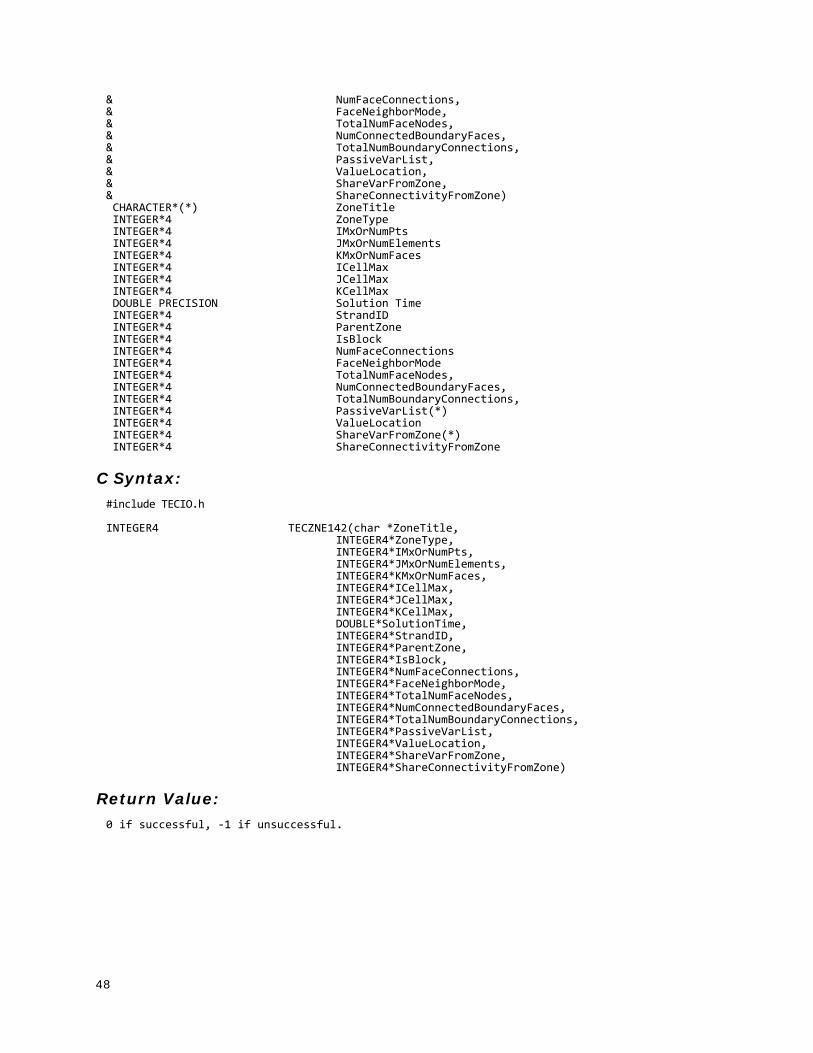
48
& NumFaceConnections,& FaceNeighborMode,& TotalNumFaceNodes,& NumConnectedBoundaryFaces,& TotalNumBoundaryConnections,& PassiveVarList,& ValueLocation,& ShareVarFromZone,& ShareConnectivityFromZone) CHARACTER*(*) ZoneTitle INTEGER*4 ZoneType INTEGER*4 IMxOrNumPts INTEGER*4 JMxOrNumElements INTEGER*4 KMxOrNumFaces INTEGER*4 ICellMax INTEGER*4 JCellMax INTEGER*4 KCellMax DOUBLE PRECISION Solution Time INTEGER*4 StrandID INTEGER*4 ParentZone INTEGER*4 IsBlock INTEGER*4 NumFaceConnections INTEGER*4 FaceNeighborMode INTEGER*4 TotalNumFaceNodes, INTEGER*4 NumConnectedBoundaryFaces, INTEGER*4 TotalNumBoundaryConnections, INTEGER*4 PassiveVarList(*) INTEGER*4 ValueLocation INTEGER*4 ShareVarFromZone(*) INTEGER*4 ShareConnectivityFromZone
C Syntax:#include TECIO.h
INTEGER4 TECZNE142(char *ZoneTitle,INTEGER4*ZoneType,INTEGER4*IMxOrNumPts,INTEGER4*JMxOrNumElements,INTEGER4*KMxOrNumFaces,INTEGER4*ICellMax,INTEGER4*JCellMax,INTEGER4*KCellMax,DOUBLE*SolutionTime,INTEGER4*StrandID,INTEGER4*ParentZone,INTEGER4*IsBlock,INTEGER4*NumFaceConnections,INTEGER4*FaceNeighborMode,INTEGER4*TotalNumFaceNodes,INTEGER4*NumConnectedBoundaryFaces,INTEGER4*TotalNumBoundaryConnections,INTEGER4*PassiveVarList,INTEGER4*ValueLocation,INTEGER4*ShareVarFromZone,INTEGER4*ShareConnectivityFromZone)
Return Value:0 if successful, -1 if unsuccessful.

49
Binary Data File Function Reference
Parameters:
Parameter Applies to Zone Type(s) Notes
ZoneTitle ALL The title of the zone. Must be null-terminated.
ZoneType ALL
The type of the zone: 0=ORDERED 1=FELINESEG 2=FETRIANGLE 3=FEQUADRILATERAL 4=FETETRAHEDRON5=FEBRICK6=FEPOLYGON7=FEPOLYHEDRON
IMaxorNumPts
ALLFor ordered zones, the number of nodes in the I-index direction. For finite element zones (cell-based and face-based), the number of nodes.
JMaxorNumElements
ALLFor ordered zones, the number of nodes in the J index direction. For finite element zones (cell-based and face-based), the number of elements.
KMaxorNumFaces
ORDEREDFEPOLYGONFEPOLYHEDRON
For ordered zones, the number of nodes in the K index direction. For polyhedral and polygonal finite element zones, it is the number of faces. Not used all other finite element zone types.
ICellMax N/A Reserved for future use. Set to zero.
JCellMax N/A Reserved for future use. Set to zero.
KCellMax N/A Reserved for future use. Set to zero.
SolutionTime ALL
Scalar double precision value specifying the time associated with the zone. Refer to Section 7 - 2 “Time Aware” in the User’s Manual for additional information on working with transient data.
StrandID ALL
Scalar integer value specifying the strand to which the zone is associated.
0 = static zone, not associated with a strand.Values greater than 0 indicate a zone is assigned to a given strand.
Refer to Section 7 - 2 “Time Aware” in the User’s Manual for additional information on strands.
If you are converting your function calls from function calls 109 or older, use “0” for StrandID.

50
ParentZone ALL
Scalar integer value representing the relationship between this zone and its parent. With a parent zone association, Tecplot 360 can generate a surface streamtrace on a no-slip boundary zone. A zone may not specify itself as its own parent.
0 = indicates that this zone is not associated with a parent zone.>0 = A value greater than zero is considered this zone's parent.
Refer to Section 7 - 2 “Time Aware” in the User’s Manual for additional information on parent zones and Section 15 - 2 “Surface Streamtraces on No-slip Boundaries” in the User’s Manual for additional information regarding no-slip boundaries.
IsBlock ALL
Indicates that data will be passed into TECDAT142 in BLOCK format. Always use 1 to indicate the BLOCK format, as TecZne functions do not output in point format.
NumFaceConnections
ORDERED FELINESEG FETRIANGLE FEQUADRILATERALFETETRAHEDRONFEBRICK
Used for cell-based finite element and ordered zones only. The number of face connections that will be passed in routine TECFACE142.
FaceNeighborMode
ORDERED FELINESEG FETRIANGLE FEQUADRILATERALFETETRAHEDRONFEBRICK
Used for cell-baseda finite element and ordered zones only. The type of face connections that will be passed in routine TECFACE142.
0=LocalOneToOne 2=GlobalOneToOne1=LocalOneToMany 3=GlobalOneToMany
TotalNumFaceNodes FEPOLYGONFEPOLYHEDRON
Used for face-basedb finite element zones. Total number of nodes for all faces. It is also the sum of the FaceNodeCounts array (defined in TECPOLY142). For polygonal zones this value is equivalent to 2 * NumFaces. NumFaces = the number of faces in the zone. Refer to Section 3 - 8.2 “FaceNodeCounts and FaceNodes” for simple example.
NumConnectedBoundaryFaces FEPOLYGONFEPOLYHEDRON
Used for face-basedb finite element zones. Total number of boundary faces, where boundary faces are faces that either have more than one neighboring cell on a side or have a neighboring cell from another zone. Refer to Section 3 - 8.1 “Boundary Faces and Boundary Connections” for simple example.
Parameter Applies to Zone Type(s) Notes

51
Binary Data File Function Reference
Examples:Refer to the following examples for illustrations of working with TECZNE142:
• Section 2 - 4 “Face Neighbors”• Section 3 - 5 “Writing to Multiple Binary Data Files”• Section 3 - 9.2 “Polygonal Example”• Section 3 - 9.3 “Multiple Polyhedral Zones”• Section 3 - 9.4 “Multiple Polygonal Zones”• Section 3 - 9.5 “Polyhedral Example”
TotalNumBoundaryConnections
FEPOLYGONFEPOLYHEDRON
Used for face-basedb finite element zones. Total number of boundary connections for all faces. In general, TotalNumBoundaryConnections will be equal to NumConnectedBoundaryFaces. However, TotalNumBoundaryConnections must be greater than or equal to NumConnectedBoundaryFaces. Refer to Section 3 - 8.1 “Boundary Faces and Boundary Connections” for simple example.
PassiveVarList ALL
Array, dimensioned by the number of variables, of 4 byte integer values specifying the active/passive nature of each variable. A value of 0 indicates the associated variable is active while a value of 1 indicates that it is passive. If all variables are active, you may pass NULL rather than an array of zeroes. Refer to “Passive Variables” on page 9 for additional information.
ValueLocation ALL
The location of each variable in the data set. ValueLocation(I) indicates the location of variable I for this zone. 0=cell-centered, 1=node-centered. Pass null to indicate that all variables are node-centered.
ShareVarFromZone ALL
Indicates variable sharing. Array, dimensioned by the number of variables. ShareVarFromZone(I) indicates the zone number with which variable I will be shared. This reduces the amount of data to be passed via TECDAT142. A value of 0 indicates that the variable is not shared. Pass null to indicate no variable sharing for this zone. You must pass null for the first zone in a data set (there is no data available to share).
ShareConnectivityFromZone ALL
Indicates the zone number with which connectivity is shared. Pass 0 to indicate no connectivity sharing. You must pass 0 for the first zone in a data set. NOTE: Connectivity and/or face neighbors cannot be shared when the face neighbor mode is set to Global. Connectivity cannot be shared between cell-based and face-based finite element zones.
a. Cell-based finite element zones: FELINESEG, FETRIANGLE, FEQUADRILATERAL, FETETRAHEDRON, and FEBRICK.
b. Face-based finite element zones: FEPOLYGON and FEPOLYHEDRON.
Parameter Applies to Zone Type(s) Notes

52
3 - 8 Defining Polyhedral and Polygonal DataPolyhedral data is defined using TECPOLY142 (or TECPOLYFACE142/TECPOLYBCONN142) and TECZNE142. Via TECZNE142 the number of nodes, faces, elements, boundary faces, and boundary connections are specified. TECPOLY142 is used to specify the face mapping connections for the zone.
Before defining your polyhedral or polygonal data, you should determine the numbering scheme for the nodes, faces and elements in each zone of your data set. The numbering scheme is communicated to Tecplot implicitly by the order in which you supply the data. For example, the first nodal value supplied is for Node 1, followed by the value for Node 2, continuing to node N (where N is the total number of nodes). Similarly, for faces and elements.
The remainder of this section provides simple examples illustrating how to define polygonal and polyhedral data.
3 - 8.1 Boundary Faces and Boundary ConnectionsA “Connected Boundary Face” is a face with at least one neighboring element that belongs to another zone. Each “Connected Boundary Face” has one or more “Boundary Connections”. A “Boundary Connection” is defined as the element-zone tuple used to identify the neighboring element when the element is part of another zone.
Consider the following picture:
In the figure shown above, Zone 1 contains a single element (e1) and Zone 2 contains two elements (e1 and e2). The boundary faces and boundary connections for each zone are as follows:
• Zone 1 - In Zone 1, Face 1 (f1) is the sole connected boundary face. It has two boundary connections. The first boundary connection is Element 1 in Zone 2. The second boundary connection is Element 2 in Zone 2.
• NumConnectedBoundaryFaces = 1• TotalNumBndryConnections = 2
• Zone 2 - In Zone 2, both Face 1 and Face 2 are connected boundary faces. There is a total of two boundary connections. The boundary connection for each boundary face in Zone 2 is Element 1 in Zone 1.
• NumConnectedBoundaryFaces = 2• TotalNumBndryConnections = 2
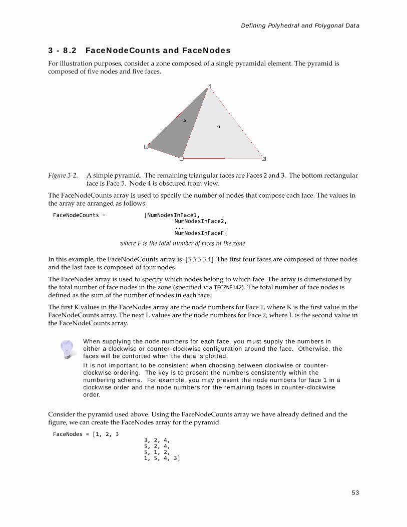
53
Defining Polyhedral and Polygonal Data
3 - 8.2 FaceNodeCounts and FaceNodesFor illustration purposes, consider a zone composed of a single pyramidal element. The pyramid is composed of five nodes and five faces.
Figure 3-2. A simple pyramid. The remaining triangular faces are Faces 2 and 3. The bottom rectangular face is Face 5. Node 4 is obscured from view.
The FaceNodeCounts array is used to specify the number of nodes that compose each face. The values in the array are arranged as follows:
FaceNodeCounts = [NumNodesInFace1, NumNodesInFace2, ... NumNodesInFaceF]
where F is the total number of faces in the zone
In this example, the FaceNodeCounts array is: [3 3 3 3 4]. The first four faces are composed of three nodes and the last face is composed of four nodes.
The FaceNodes array is used to specify which nodes belong to which face. The array is dimensioned by the total number of face nodes in the zone (specified via TECZNE142). The total number of face nodes is defined as the sum of the number of nodes in each face.
The first K values in the FaceNodes array are the node numbers for Face 1, where K is the first value in the FaceNodeCounts array. The next L values are the node numbers for Face 2, where L is the second value in the FaceNodeCounts array.
Consider the pyramid used above. Using the FaceNodeCounts array we have already defined and the figure, we can create the FaceNodes array for the pyramid.
FaceNodes = [1, 2, 33, 2, 4,5, 2, 4,5, 1, 2,1, 5, 4, 3]
When supplying the node numbers for each face, you must supply the numbers in either a clockwise or counter-clockwise configuration around the face. Otherwise, the faces will be contorted when the data is plotted. It is not important to be consistent when choosing between clockwise or counter-clockwise ordering. The key is to present the numbers consistently within the numbering scheme. For example, you may present the node numbers for face 1 in a clockwise order and the node numbers for the remaining faces in counter-clockwise order.

54
3 - 8.3 FaceRightElems and FaceLeftElemsAfter specifying the face map data (using the FaceNodeCounts and FaceNodes array), the next step is to identify the element on either side of each face. To illustrate this, we will switch from the single element zone to the following data set:
The neighboring elements can be determined using the right-hand rule:
• 2D Data - For each face, place your right-hand along the face with your fingers pointing in the direction of incrementing node numbers (i.e. from Node 1 to Node 2). The right side of your hand will indicate the right element, and the left side of your hand will indicate the left element.
• 3D Data - For each face, curl the fingers of your right-hand following the order that the nodes were presented in the FaceNodes array. Your thumb will point to the right element. The left element is the other adjacent element. If the face has more than one neighboring element on a single side, you will need to use the FaceBoundaryConnectionCounts, FaceBoundaryConnectionElems and FaceBoundaryConnectionZones array.
The neighboring elements for each face are stored in the FaceRightElems and FaceLeftElems array. Each array is dimensioned by the total number of faces in the zone. The first value in each array is the right or left neighboring element for Face 1, followed by the neighboring element for Face 2, and so forth.
FaceRightElems = [RightNeighborToFace1, RightNeighborToFace2, ... RightNeighborToFaceF]
FaceLeftElems = [LeftNeighborToFace1, LeftNeighborToFace2, ... LeftNeighborToFaceF]
where F is the total number of faces
In the above plot, the face neighbors are as follows:
Face Number Right Neighboring Element
Left Neighboring Element
Face 1 1 0
Face 2 1 0
Face 3 1 2
Face 4 1 3

55
Defining Polyhedral and Polygonal Data
The number zero is used to indicate that the face is on the edge of the data (i.e. has “no neighboring element”).
3 - 8.4 FaceBoundaryConnectionElements and ZonesWhen working with multiple zones, an additional aspect is folded into the FaceLeftElems and FaceRightElems arrays. When the neighboring element is not within the current zone, you cannot identify the element by its element number alone. Instead you need to specify both the element number and its zone number. This is accomplished using the FaceBoundaryConnectionElements and FaceBoundaryConnectionZones arrays. For each boundary connection, the element number of the boundary connection is stored in the FaceBoundaryConnectionElements array while its zone number is stored in the FaceBoundaryConnectionZones array.
A negative value in the FaceLeftElems or FaceRightElems array is used to indicate that the neighboring element belongs to another zone. The magnitude of the negative number is a pointer to a value in the FaceBoundaryConnectionElements and FaceBoundaryConnectionZones arrays. For example, given the following FaceBoundaryConnectionElements and FaceBoundaryConnectionZones arrays:
FaceBoundaryConnectionElements = [ 1 1 3 4 ]FaceBoundaryConnectionZones = [ 2 2 3 3 ]
A value of -4 in the FaceLeftElems indicates that the left neighboring element for that face is element four in zone three.
3 - 8.5 Partially Obscured Boundary FacesA face on the boundary of a zone may be partially obscured by its boundary connections (neighboring elements). While Tecplot 360 does not draw fully obscured boundary faces (because it treats those faces as internal faces), Tecplot 360 does draw partially obscured boundary faces. Thus, Tecplot 360 requires definition of partially obscured boundary faces.
To indicate a partially obscured face, indicate the appropriate neighboring element as zero in the FaceBndryConnectionElems and FaceBndryConnectionZones arrays, followed by the actual neighboring elements. When Tecplot 360 sees a list of neighboring elements for a boundary face that begin with element zero, it marks that boundary face as partially obscured.
Face 5 1 4
Face 6 1 0
Face 7 2 0
Face 8 2 0
Face 9 2 0
Face 10 2 3
Face 11 3 0
Face 12 3 4
Face 13 4 0
Face 14 4 0
Face 15 4 0
Face Number Right Neighboring Element
Left Neighboring Element

56
If Tecplot 360 sees a zero in FaceBndryConnectionElems that is not the first boundary element listed for a face, an error message will appear, indicating that either the partially obscured boundary face was not indicated correctly, or FaceBndryConnectionsElems and/or FaceBndryConnectionsZones was not completely filled out.
3 - 9 ExamplesThe following examples (written in C) provide a basic illustration of creating a *.plt file using the TecIO library. If you plan to compile the examples, be sure to review the instructions in Section 3 - 6 “Linking with the TecIO Library” first.
In order to keep the examples as simple as possible, error checking is not included. For complete details on the parameters used and the function syntax for each TecIO function, refer to Section 3 - 7 “Binary Data File Function Reference”. When creating a binary data file using the TecIO library, the functions must be called in a specific order. Refer to Section 3 - 4 “Binary Data File Function Calling Sequence” for details.
3 - 9.1 Face NeighborsThis example illustrates how to (1) create two simple FE-quadrilateral zones and (2) create a face neighbor connection between the two zones. In order to keep the example as simple as possible, error checking is not included. If you plan to compile this example, be sure to include TECIO.h.
For complete details on the parameters used and the function syntax for each TecIO function, refer to Section 3 - 7 “Binary Data File Function Reference”. When creating a binary data file using the TecIO library, the functions must be called in a specific order. Refer to Section 3 - 4 “Binary Data File Function Calling Sequence” for details.
Step 1 Initialize the data file using TECINITECINI is required for all data files. It is used to: open the data file and initialize the file header information (name the data file, the variables for the data file, and the file type).
INTEGER4 Debug = 1;INTEGER4 VIsDouble = 0;INTEGER4 FileType = 0;INTEGER4 FileFormat = 0; // 0 == PLT, 1 == SZPLTINTEGER4 I = 0; /* Used to track return codes */
I = TECINI142((char*)”Face Neighbors Example”, /* Specifies the name * of the entire * dataset */ (char*)”X Y P”, /* Defines the * variables for the * data file. Each * zone must contain * each of the vars * listed. The order * of the variables in * the list is used to * define the variable * number (e.g. X is * Var 1.) */
(char*)”FaceNeighbors.plt”, /* Specifies the * file name. */ (char*)”.”, &FileFormat,

57
Examples
Step 2 Create Zone 1After TECINI is called, call TECZNE to create one or more zones for your data file.
&FileType, /* The FileType is set to * zero, indicating it is * a full file (containing * both grid and solution * data). */ &Debug, &VIsDouble);
INTEGER4 ZoneType = 3; /* set the zone type to * FEQuadrilateral */INTEGER4 NumPts = 6;INTEGER4 NumElems = 2;INTEGER4 NumFaces = 8;INTEGER4 ICellMax = 0; /* not used */INTEGER4 JCellMax = 0; /* not used */INTEGER4 KCellMax = 0; /* not used */double SolTime = 360.0;INTEGER4 StrandID = 0; /* StaticZone */INTEGER4 ParentZn = 0;INTEGER4 IsBlock = 1; /* Block */INTEGER4 NFConns = 1; /* Specify the number of Face * Neighbor Connections in the * Zone. When this value is * greater than zero, TECFACE must * be called prior to creating the * next zone or ending the file. */
/* Specify the Face Neighbor Mode. * A value of 2 indicated that the face neighbor mode is global * one-to-one. The scope of the face neighbors (local or * global) is with respect to the zones. A value of global * indicates that the face neighbor(s) is/are shared aross zones; * a value of local indicates that the face neighbor(s) are * shared within the current zone. The terms one-to-one and * one-to-many are used to indicate whether the face in question * is shared with one cell or several cells. * For example, if your data is arranged as follows:
----------------------- | | | | | 1 | 2 | 3 | | | | | ----------------------- | | | | 4 | 5 | | | | ----------------------- * The face between 1 & 4 is local-one-to-one. The face between * 5 and (2 & 3) is local one-to-many. */
INTEGER4 FNMode = 2;
INTEGER4 TotalNumFaceNodes = 1; /* Not used for * FEQuad zones*/INTEGER4 NumConnectedBoundaryFaces = 1; /* Not used for

58
Step 3 Define the node numbering for Zone 1For this example, we will create 2 rectangular cells in Zone 1. Before defining your variables, you must establish a consistent node numbering scheme for your data. Once the node numbers are defined, supply the variable values in the node numbering order. In this example, Node 1 is defined at X = 0 and Y = 0. As such, the first value supplied for X (i.e. X[0]) is 0. Similarly, the first value supplied for Y is 0.
* FEQuad zones*/INTEGER4 TotalNumBoundaryConnections = 1; /* Not used for * FEQuad zones*/INTEGER4 ShrConn = 0;
INTEGER4 ValueLocation[3] = {1, 1, 1}; /* Specify the variable * values at the nodes. * NOTE: Because all of * the variables are * defined at the nodes, * we can just pass * NULL for this array. * We are providing the * array for illustration * purposes. */
I = TECZNE142((char*)”Zone 1”, &ZoneType, &NumPts, &NumElems, &NumFaces, &ICellMax, &JCellMax, &KCellMax, &SolTime, &StrandID, &ParentZn, &IsBlock, &NFConns, &FNMode, &TotalNumFaceNodes, &NumConnectedBoundaryFaces, &TotalNumBoundaryConnections, NULL, ValueLocation, NULL, &ShrConn);
It is important that you refer to node numbers consistently. The node numbers will be used later to define the connectivity for each element.
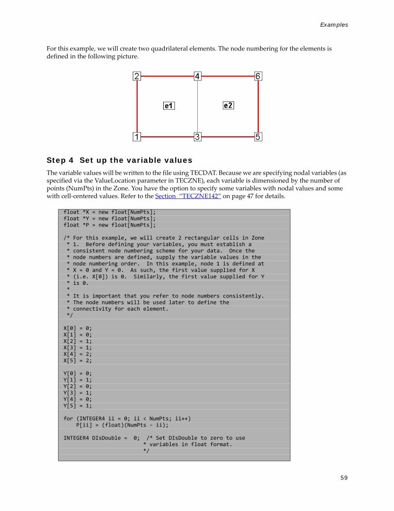
59
Examples
For this example, we will create two quadrilateral elements. The node numbering for the elements is defined in the following picture.
Step 4 Set up the variable valuesThe variable values will be written to the file using TECDAT. Because we are specifying nodal variables (as specified via the ValueLocation parameter in TECZNE), each variable is dimensioned by the number of points (NumPts) in the Zone. You have the option to specify some variables with nodal values and some with cell-centered values. Refer to the Section “TECZNE142” on page 47 for details.
float *X = new float[NumPts];float *Y = new float[NumPts];float *P = new float[NumPts];
/* For this example, we will create 2 rectangular cells in Zone * 1. Before defining your variables, you must establish a * consistent node numbering scheme for your data. Once the * node numbers are defined, supply the variable values in the * node numbering order. In this example, node 1 is defined at * X = 0 and Y = 0. As such, the first value supplied for X * (i.e. X[0]) is 0. Similarly, the first value supplied for Y * is 0. * * It is important that you refer to node numbers consistently. * The node numbers will be used later to define the * connectivity for each element. */
X[0] = 0;X[1] = 0;X[2] = 1;X[3] = 1;X[4] = 2;X[5] = 2;
Y[0] = 0;Y[1] = 1;Y[2] = 0;Y[3] = 1;Y[4] = 0;Y[5] = 1;
for (INTEGER4 ii = 0; ii < NumPts; ii++) P[ii] = (float)(NumPts - ii);
INTEGER4 DIsDouble = 0; /* Set DIsDouble to zero to use * variables in float format. */

60
Step 5 Define the connectivity list for Zone 1 The Connectivity List is used to specify the nodes that compose each element. When working with nodal variables, the numbering of the nodes is implicitly defined when the variables are declared. The first value of each variable is for node one, the second value for node two, and so on.
Because this zone contains two quadrilateral elements, we must supply 8 values in the connectivity list. The first four values define the nodes that form Element 1. Similarly, the second four values define the nodes that form Element 2.
Step 6 Define the face neighbor connections for Zone 1Now that TECNOD or TECNODE has been called, the creation of Zone 1 is complete. However, in this example, we will define a face neighbor between Zone 1 and Zone 2 (to be created later in the example). Face Neighbor connections are used to define connections that are not created via the connectivity list. For example, local face neighbors may need to be defined when a zone wraps onto itself and global face neighbors may need to be defined to smooth edges across zones. Face Neighbors are used when deriving variables and drawing contours.
In this example, we are creating a face neighbor connection between Cell 2 in Zone 1 and Cell 1 in Zone 2. The information required when specifying face neighbors depends upon the type of connection. Refer to Section “TECFACE142” on page 26 for details.
In this case, we must supply the following information (in the order provided):
• the cell number in the current zone that contains the face neighbor• the number of the face in that cell that contains the face neighbor
/* Call TECDAT once for each variable */I = TECDAT142(&NumPts, &X[0], &DIsDouble);I = TECDAT142(&NumPts, &Y[0], &DIsDouble);I = TECDAT142(&NumPts, &P[0], &DIsDouble);
INTEGER4 ConnList[8] = {1, 3, 4, 2, 3, 5, 6, 4 };I = TECNOD142(ConnList);
It is important to provide the node list in either a clockwise or counter-clockwise order. Otherwise, your elements will be misshapen. For example, if the first two numbers in the above connectivity list were switched, the zone would appear as follows:
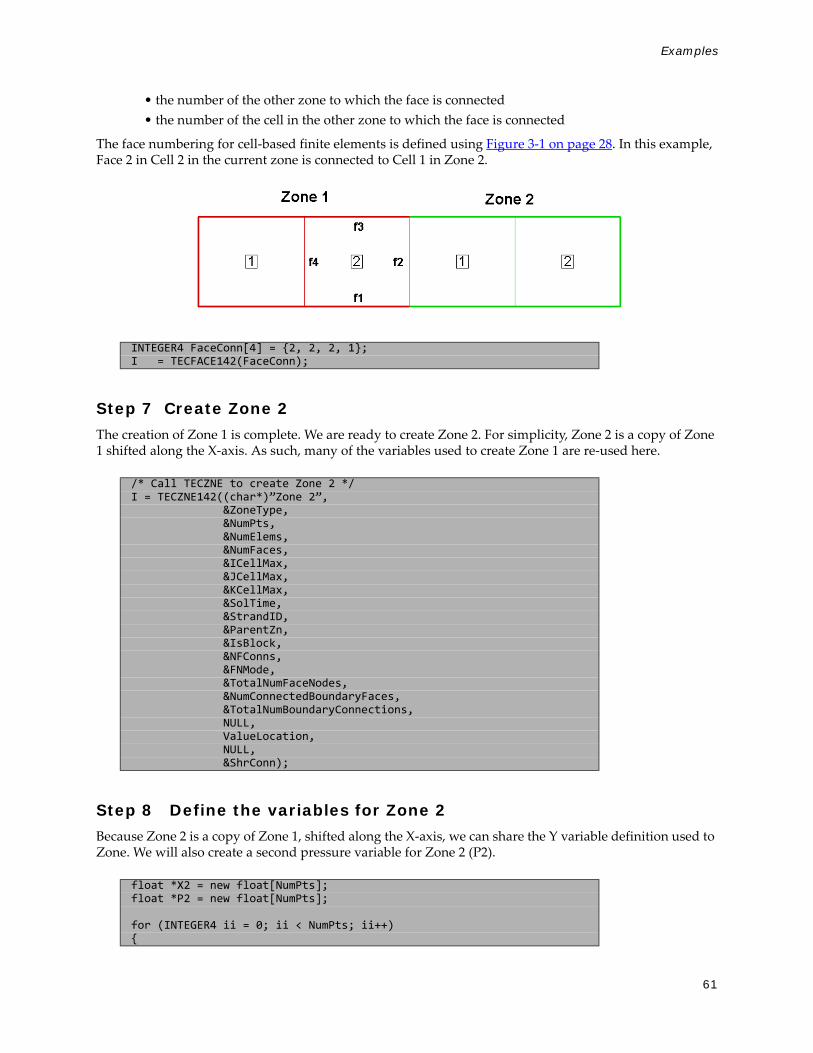
61
Examples
• the number of the other zone to which the face is connected• the number of the cell in the other zone to which the face is connected
The face numbering for cell-based finite elements is defined using Figure 3-1 on page 28. In this example, Face 2 in Cell 2 in the current zone is connected to Cell 1 in Zone 2.
Step 7 Create Zone 2The creation of Zone 1 is complete. We are ready to create Zone 2. For simplicity, Zone 2 is a copy of Zone 1 shifted along the X-axis. As such, many of the variables used to create Zone 1 are re-used here.
Step 8 Define the variables for Zone 2Because Zone 2 is a copy of Zone 1, shifted along the X-axis, we can share the Y variable definition used to Zone. We will also create a second pressure variable for Zone 2 (P2).
INTEGER4 FaceConn[4] = {2, 2, 2, 1};I = TECFACE142(FaceConn);
/* Call TECZNE to create Zone 2 */I = TECZNE142((char*)”Zone 2”, &ZoneType, &NumPts, &NumElems, &NumFaces, &ICellMax, &JCellMax, &KCellMax, &SolTime, &StrandID, &ParentZn, &IsBlock, &NFConns, &FNMode, &TotalNumFaceNodes, &NumConnectedBoundaryFaces, &TotalNumBoundaryConnections, NULL, ValueLocation, NULL, &ShrConn);
float *X2 = new float[NumPts];float *P2 = new float[NumPts];
for (INTEGER4 ii = 0; ii < NumPts; ii++){

62
Step 9 Define the connectivity list for Zone 2As with Zone 1, we must define the connectivity list for Zone 2. Because, the node numbering restarts at one for each new zone and the nodal arrangement is identical between the two zones, we may reuse the connectivity list from Zone 1.
Step 10 Define the face neighbor connections for Zone 2We will now specify the face neighbor connection with respect to our new current zone of Zone 2.
Step 11 Close the fileCall TECEND to close the file.
X2[ii] = X[ii] + 2; P2[ii] = 2 * (float)ii;}
I = TECDAT142(&NumPts, &X2[0], &DIsDouble);I = TECDAT142(&NumPts, &Y[0], &DIsDouble);I = TECDAT142(&NumPts, &P2[0], &DIsDouble);
delete X;delete Y;delete P;delete X2;delete P2;
I = TECNOD142(ConnList);
INTEGER4 FaceConn2[4] = {1, 4, 1, 2}; /* cell 1, face 4 in * current zone is a * neighbor to cell 2 in * zone 1. */I = TECFACE142(FaceConn2);
I = TECEND142();
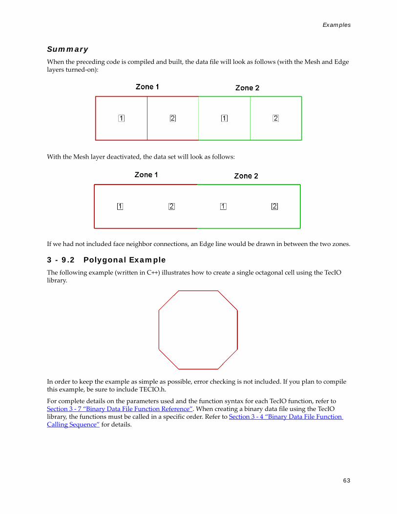
63
Examples
SummaryWhen the preceding code is compiled and built, the data file will look as follows (with the Mesh and Edge layers turned-on):
With the Mesh layer deactivated, the data set will look as follows:
If we had not included face neighbor connections, an Edge line would be drawn in between the two zones.
3 - 9.2 Polygonal ExampleThe following example (written in C++) illustrates how to create a single octagonal cell using the TecIO library.
In order to keep the example as simple as possible, error checking is not included. If you plan to compile this example, be sure to include TECIO.h.
For complete details on the parameters used and the function syntax for each TecIO function, refer to Section 3 - 7 “Binary Data File Function Reference”. When creating a binary data file using the TecIO library, the functions must be called in a specific order. Refer to Section 3 - 4 “Binary Data File Function Calling Sequence” for details.

64
Step 1 Initialize the data file using TECINITECINI is required for all data files. It is used to: open the data file and initialize the file header information (name the data file, the variables for the data file, and the file type).
Step 2 Create Zone 1After TECINI is called, call TECZNE to create one or more zones for your data file.
INTEGER4 Debug = 1;INTEGER4 VIsDouble = 0;INTEGER4 FileType = 0;INTEGER4 FileFormat = 0; // 0 == PLT, 1 == SZPLT; Only PLT is currently // supported for polygonal zones.INTEGER4 I; /* used to check return codes */
/* * Open the file and write the Tecplot datafile * header information */
I = TECINI142((char*)”Octagon”, (char*)”X Y P”, /* Defines the variables for the data * file. Each zone must contain each * of the vars listed here. The order * of the variables in the list is * used to define the variable number * (e.g. X is Variable 1). When * referring to variables in other * TecIO functions, you will refer to * thevariable by its number. */ (char*)”Octagon.plt”, (char*)”.”, /* scratch directory */ &FileFormat, &FileType, &Debug, &VIsDouble);
/* In this example, we will create a single octagonal cell in * Tecplot 360’s polyhedral file format. */INTEGER4 ZoneType = 6; /* FEPolygon */INTEGER4 NumNodes = 8; /* Number of nodes in the octagon.*/INTEGER4 NumElems = 1; /* Number of octagonal elements. */INTEGER4 NumFaces = 8; /* Number of faces in the octagon.*/INTEGER4 ICellMax = 0; /* Not Used */INTEGER4 JCellMax = 0; /* Not Used */INTEGER4 KCellMax = 0; /* Not Used */double SolTime = 360.0;INTEGER4 StrandID = 0; /* Static Zone */INTEGER4 ParentZn = 0; /* No Parent Zone */INTEGER4 IsBlock = 1; /* Block */INTEGER4 NFConns = 0;INTEGER4 FNMode = 0;
/* For polygonal zones, the total number of face nodes is equal * to twice the number of nodes. This is because, each face * has exactly two nodes. */INTEGER4 NumFaceNodes = 2 * NumNodes;

65
Examples
Step 3 Define node numberingFor this example, we will create a single octagonal cell. Before defining your variables, you must establish a consistent node numbering scheme for your data. Once the node numbers are defined, supply the variable values in the node numbering order. In this example, Node 1 is defined at X = .25 and Y = 0. As such, the first value supplied for X (i.e. X[0]) is .25. Similarly, the first value supplied for Y is 0.
It is important that you refer to node numbers consistently. The node numbers will be used later to define the connectivity for each element.
/* Boundary Faces and Boundary Connections are not used in this * example. */INTEGER4 NumBFaces = 0;INTEGER4 NumBConnections = 0;
INTEGER4 ShrConn = 0;
I = TECZNE142((char*)”Octagonal Zone”, &ZoneType, &NumNodes, &NumElems, &NumFaces, &ICellMax, &JCellMax, &KCellMax, &SolTime, &StrandID, &ParentZn, &IsBlock, &NFConns, &FNMode, &NumFaceNodes, &NumBFaces, &NumBConnections, NULL, NULL, /* When Value Location is not specified, * Tecplot will treat all variables as * nodal variables. */ NULL, &ShrConn);

66
Step 4 Set up the variable values Write the variable values to the file using TECDAT. Because we are specifying nodal variables (as specified via the ValueLocation parameter in TECZNE), each variable is dimensioned by the number of points (NumPts) in the Zone. You have the option to specify some variables with nodal values and some with cell-centered values. Refer to Section “TECZNE142” on page 47 for details.
The order of the values supplied for each nodal variable is determined by the node numbering established in Step 3. The first value for each variable is for Node 1, the second value for each variable is for Node 2 and so forth.
V1 = {ValueAtNode1, ValueAtNode2, ..., ValueAtNodeN}
where N is the total number of nodes
float *X = new float[NumNodes];float *Y = new float[NumNodes];float *P = new float[NumNodes];
//Define the grid values.X[0] = 0.25;Y[0] = 0.0;
X[1] = 0.75;Y[1] = 0.0;
X[2] = 1.0;Y[2] = 0.25;
X[3] = 1.0;Y[3] = 0.75;
X[4] = 0.75;Y[4] = 1.0;
X[5] = 0.25;Y[5] = 1.0;
X[6] = 0.0;Y[6] = 0.75;
X[7] = 0.0;Y[7] = 0.25;
for (INTEGER4 ii = 0; ii < 8; ii++) P[ii] = .5;
/* Write out the field data using TECDAT */INTEGER4 DIsDouble = 0; /* set IsDouble to 0 to use float * variables. */
I = TECDAT142(&NumNodes, X, &DIsDouble);I = TECDAT142(&NumNodes, Y, &DIsDouble);I = TECDAT142(&NumNodes, P, &DIsDouble);
delete X;delete Y;delete P;

67
Examples
Step 5 Define the Face NodesThe FaceNodes array is used to indicate which nodes define which face. As mentioned earlier, the number of the nodes is implicitly defined by the order in which the nodal data is provided. The first value of each nodal variable describes Node 1, the second value describes Node 2, and so on.
The face numbering is also implicitly defined. Because there are two nodes in each face of any polygonal zone, the first two nodes provided define Face 1, the next two define Face 2 and so on. If there was a variable number of nodes used to define the faces, the array would be more complicated. Refer to Section 3 - 9.4 “Multiple Polygonal Zones” for an example.
The following picture describes the face numbering for this example:
As you can see, Face 1 is defined by Nodes 1 and 2, Face 2 is defined by Nodes 2 and 3, and so forth. Because of this simple arrangement, we can use a for-loop to define all but the end points of the face nodes array.
Step 6 Define the right and left elements of each faceThe last step for writing out the polygonal data is to define the right and left neighboring elements for each face. The neighboring elements can be determined using the right-hand rule. For each face, place your right-hand along the face with your fingers pointing the direction of incrementing node numbers (i.e. from Node 1 to Node 2). The right side of your hand will indicate the right element, and the left side of your hand will indicate the left element. Refer to Section 3 - 8.3 “FaceRightElems and FaceLeftElems” for details.
The number zero is used to indicate that there isn't an element on that side of the face (i.e. the face is on the edge of the data set). This is referred to as “no neighboring element”.
INTEGER4 *FaceNodes = new INTEGER4[NumFaceNodes];
/* * Loop over number of sides, and set each side to two * consecutive nodes. */for (INTEGER4 ii = 0; ii < 8; ii++){ FaceNodes[2*ii] = ii + 1; FaceNodes[2*ii+1] = ii + 2;}FaceNodes[15] = 1;
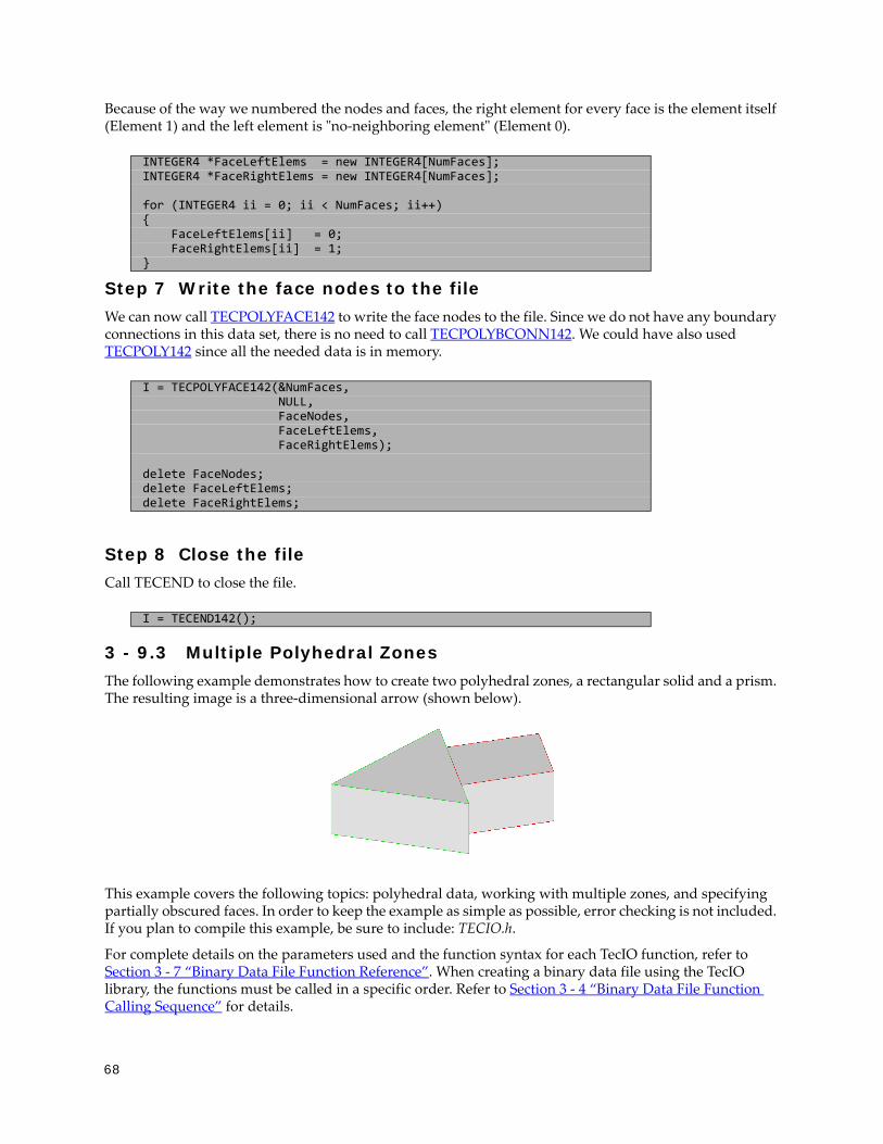
68
Because of the way we numbered the nodes and faces, the right element for every face is the element itself (Element 1) and the left element is "no-neighboring element" (Element 0).
Step 7 Write the face nodes to the fileWe can now call TECPOLYFACE142 to write the face nodes to the file. Since we do not have any boundary connections in this data set, there is no need to call TECPOLYBCONN142. We could have also used TECPOLY142 since all the needed data is in memory.
Step 8 Close the fileCall TECEND to close the file.
3 - 9.3 Multiple Polyhedral ZonesThe following example demonstrates how to create two polyhedral zones, a rectangular solid and a prism. The resulting image is a three-dimensional arrow (shown below).
This example covers the following topics: polyhedral data, working with multiple zones, and specifying partially obscured faces. In order to keep the example as simple as possible, error checking is not included. If you plan to compile this example, be sure to include: TECIO.h.
For complete details on the parameters used and the function syntax for each TecIO function, refer to Section 3 - 7 “Binary Data File Function Reference”. When creating a binary data file using the TecIO library, the functions must be called in a specific order. Refer to Section 3 - 4 “Binary Data File Function Calling Sequence” for details.
INTEGER4 *FaceLeftElems = new INTEGER4[NumFaces];INTEGER4 *FaceRightElems = new INTEGER4[NumFaces];
for (INTEGER4 ii = 0; ii < NumFaces; ii++){ FaceLeftElems[ii] = 0; FaceRightElems[ii] = 1;}
I = TECPOLYFACE142(&NumFaces, NULL, FaceNodes, FaceLeftElems, FaceRightElems);
delete FaceNodes;delete FaceLeftElems;delete FaceRightElems;
I = TECEND142();

69
Examples
Step 1 Initialize the data file using TECINITECINI is required for all data files. This function opens the data file and initializes the file header information (names the data file, the variables for the data file, and the file type)
Step 2 Create Zone 1 (rectangle)After TECINI is called, call TECZNE to create one or more zones for your data file. In this example, Zone 1 contains a single rectangular solid created as a face-based finite element (i.e. polyhedral zone). The zone has eight points (or nodes), six faces and one element.
INTEGER4 Debug = 1;INTEGER4 VIsDouble = 1;INTEGER4 FileFormat = 0; // 0 == PLT, 1 == SZPLT; Only PLT is currently // supported for ployhedral zonesINTEGER4 FileType = 0;INTEGER4 I;
/* Open the file and write the Tecplot datafile * header information */I = TECINI142((char*)”Multiple polyhedral zones”, /* Name of the entire * dataset. */ (char*)”X Y Z P”, /* Defines the variables for the data * file. Each zone must contain each of * the variables listed here. The order * of the variables in the list is used * to define the variable number (e.g. * X is Var 1). */ (char*)”Arrow.plt”, (char*)”.”, /* Scratch Directory */ &FileFormat, &FileType, &Debug, &VIsDouble);
/* TECZNE Parameters */INTEGER4 ZoneType = 7; /* sets the zone type * to polyhedral */INTEGER4 NumPts_Rect = 8;INTEGER4 NumElems_Rect = 1;INTEGER4 NumFaces_Rect = 6;INTEGER4 ICellMax = 0; /* not used */INTEGER4 JCellMax = 0; /* not used */INTEGER4 KCellMax = 0; /* not used */double SolutionTime = 0.0;INTEGER4 StrandID = 0;INTEGER4 ParentZone = 0;INTEGER4 IsBlock = 1;INTEGER4 NumFaceConnections = 0; /* not used */

70
Step 3 Set variable values for Zone 1 (rectangle)Now that the zone has been created, write the variable values to the file by calling TECDAT. While there are more elegant ways to define the grid coordinates for the rectangle, the values are defined explicitly for simplicity.
INTEGER4 FaceNeighborMode = 1; /* not used */INTEGER4 SharConn = 0;
/* In a rectangular solid, each face is composed of four nodes. * As such, the total number of face nodes is twenty-four (four * nodes for each of the six faces). */INTEGER4 TotalNumFaceNodes_Rect = 24;
/* There is one connected boundary face in this zone (the face on * the rectangle adjacent to the arrowhead). Refer to the Data * Format Guide for additional information. */INTEGER4 NumConnBndryFaces_Rect = 1;
/* The connected boundary face has one connection, the face on * the bottom of the arrowhead. A connection is an element-zone * tuple that indicates a neighboring element (and its zone) when * the neighboring element is in a different zone. Generally, * there will be one boundary connection for each boundary face. */INTEGER4 TotalNumBndryConns_Rect = 1;
/* For illustrative purposes, the grid variables (X, Y, and Z) * are nodal variables (i.e. ValueLocation = 1), and the pressure * variable (P) is a cell-centered variable (i.e. * ValueLocation = 0). */INTEGER4 ValueLocation[4] = { 1, 1, 1, 0 };
I = TECZNE142((char*)”Zone 1: Rectangular Solid”, &ZoneType, &NumPts_Rect, &NumElems_Rect, &NumFaces_Rect, &ICellMax, &JCellMax, &KCellMax, &SolutionTime, &StrandID, &ParentZone, &IsBlock, &NumFaceConnections, &FaceNeighborMode, &TotalNumFaceNodes_Rect, &NumConnBndryFaces_Rect, &TotalNumBndryConns_Rect, NULL, ValueLocation, NULL, &SharConn);

71
Examples
Using the picture below, define the variable values.
For nodal variables, provide the values for each variable in nodal order. Similarly, for cell-centered values, provide the variable values in cell order. The location of each variable is specified with TECZNE.
//set variable values (X_Rect, Y_Rect, Z_Rect & P_Rect)double *X_Rect = new double[NumPts_Rect];double *Y_Rect = new double[NumPts_Rect];double *Z_Rect = new double[NumPts_Rect];double *P_Rect = new double[NumElems_Rect];
for (INTEGER4 ii = 0; ii <= NumPts_Rect / 2; ii += 4){ X_Rect[ii] = 0; X_Rect[ii+1] = 3; X_Rect[ii+2] = 3; X_Rect[ii+3] = 0;
Y_Rect[ii] = 3; Y_Rect[ii+1] = 3; Y_Rect[ii+2] = 1; Y_Rect[ii+3] = 1;}
for (INTEGER4 ii = 0; ii < 4; ii++) Z_Rect[ii] = 0;
for (INTEGER4 ii = 4; ii < NumPts_Rect; ii++) Z_Rect[ii] = -2;
P_Rect[0] = 10;
INTEGER4 IsDouble = 1;I = TECDAT142(&NumPts_Rect, X_Rect, &IsDouble);I = TECDAT142(&NumPts_Rect, Y_Rect, &IsDouble);I = TECDAT142(&NumPts_Rect, Z_Rect, &IsDouble);I = TECDAT142(&NumElems_Rect, P_Rect, &IsDouble);

72
Step 4 Define the facemap data for Zone 1Using the following figure, specify which nodes define which face.
Figure 3-3. Zone 2 of the sample data. Node 7 is obscured from view and located in the back-left hand corner. Face 6 is the bottom face. Face 3 is opposite Face 1 and Face 4 is opposite Face 2.
In order to specify the face map data, you must first specify how many nodes are in each face using the FaceNodeCounts array. After defining the FaceNodeCounts array, use the FaceNodes array to identify the nodes that compose each face. Refer to Section 3 - 8.2 “FaceNodeCounts and FaceNodes” for additional information.
/* The FaceNodeCounts array is used to describe the number of * nodes in each face of the zone. The first value in the array * is the number of nodes in Face 1, the second value is the * number of nodes in Face 2 and so forth. In this example, each * face of the zone has four nodes. */
INTEGER4 *FaceNodeCounts_Rect = new INTEGER4[NumFaces_Rect];//For this particular zone, each face has the 4 nodesfor (INTEGER4 ii = 0; ii < NumFaces_Rect; ii++) FaceNodeCounts_Rect[ii] = 4;
/* The FaceNodes array is used to specify the nodes that compose * each face. For each face (n of N), the number of nodes used * to define the face is specified by the nth value in the * FaceNodeCounts array. For example, if the first value in the * FaceNodeCounts array is 4 (indicating Face 1 is composed of * four nodes), the first four values in the FaceNodes array are * the node numbers of the nodes in Face 1. * * ------------ * WARNING * When providing the node numbers for each face, you must * provide the node numbers in a consistent order (either * clockwise or counter-clockwise. Providing the node numbers * out of order results in contorted faces. * ------------ */
INTEGER4 *FaceNodes_Rect = new INTEGER4[TotalNumFaceNodes_Rect];
//Nodes for Face 1FaceNodes_Rect[0] = 1;FaceNodes_Rect[1] = 2;FaceNodes_Rect[2] = 3;FaceNodes_Rect[3] = 4;
//Nodes for Face 2FaceNodes_Rect[4] = 1;FaceNodes_Rect[5] = 4;
73
Examples
Step 5 Specify the neighboring elements for Zone 1The next step for writing out the polyhedral data is to define the right and left neighboring elements for each face. The neighboring elements can be determined using the right-hand rule. For each face, place your right-hand along the face with your fingers pointing the direction of incrementing node numbers (i.e. from Node 1 to Node 2). The right side of your hand will indicate the right element, and the left side of your hand will indicate the left element. Refer to Section 3 - 8.3 “FaceRightElems and FaceLeftElems” for details.
The number zero is used to indicate that there isn't an element on that side of the face. A negative number is used when the neighboring element is in another zone. The value of the negative number along with the FaceBndryConnectionCounts array points to the position in the FaceBoundaryConnectionElems and FaceBoundaryConnectionZones arrays that defines the element and zone numbers of the neighboring element. Refer to Step 6 for details.
Because of the way we numbered the nodes and faces, the right element for every face (except the face connected to the arrowhead) is the element itself (Element 1) and the left element is "no-neighboring element" (Element 0).
FaceNodes_Rect[6] = 8;FaceNodes_Rect[7] = 5;
//Nodes for Face 3FaceNodes_Rect[8] = 5;FaceNodes_Rect[9] = 8;FaceNodes_Rect[10] = 7;FaceNodes_Rect[11] = 6;
//Nodes for Face 4FaceNodes_Rect[12] = 2;FaceNodes_Rect[13] = 6;FaceNodes_Rect[14] = 7;FaceNodes_Rect[15] = 3;
//Nodes for Face 5FaceNodes_Rect[16] = 6;FaceNodes_Rect[17] = 2;FaceNodes_Rect[18] = 1;FaceNodes_Rect[19] = 5;
//Nodes for Face 6FaceNodes_Rect[20] = 3;FaceNodes_Rect[21] = 7;FaceNodes_Rect[22] = 8;FaceNodes_Rect[23] = 4;
When providing the node numbers for each face, you must provide the node numbers in a consistent order (either clockwise or counter-clockwise. Providing the node numbers out of order results in contorted faces.
INTEGER4 *FaceLeftElems_Rect = new INTEGER4[NumFaces_Rect];INTEGER4 *FaceRightElems_Rect = new INTEGER4[NumFaces_Rect];
/* Since this zone has just one element, all leftelems are * NoNeighboring Element and all right elems are itself */for (INTEGER4 ii = 0; ii < NumFaces_Rect; ii++){ FaceRightElems_Rect[ii] = 1;
74
After defining the face nodes, we call TECPOLYFACE to write it to the file.
Step 6 Define boundary connections for Zone 1The last step for defining the rectangular solid is to describe the boundary connections and call TECPOLYBCONN.
FaceLeftElems_Rect[ii] = 0;}
/* The negative value in the FaceLeftElems array indicates that * the face is connected to an element in another zone. In this * case, Face 4 is connected to a face in Zone 2 (to be defined * later in the example). The FaceBoundaryConnectionElems array * lists all of the element numbers in other zones that the * current zone shares boundary connections with. Similarly, the * FaceBoundaryConnectionZones array lists all of the zone numbers * with which the current zone shares boundaries. A negative * value in the FaceLeftElems or FaceRightElems array indicates * the position within these arrays that defines the neighboring * element and zone for a face. * * For example, if the FaceBoundaryConnectionElems array is: * [1 8 2] and the FaceBoundaryConnectionZones array is: [2 5 3], * a FaceLeftElems or FaceRightElems value of -2 indicates that * the face in question has a boundary connection with Element 8 * in Zone 5. */FaceLeftElems_Rect[3] = -1;
I = TECPOLYFACE142(&NumFaces_Rect, FaceNodeCounts_Rect, FaceNodes_Rect, FaceLeftElems_Rect, FaceRightElems_Rect);
/* The FaceBndryConnectionCounts array is used to define the * number of boundary connections for each face that has a * boundary connection. For example, if a zone has three boundary * connections in total (NumConnectedBoundaryFaces), two of those * boundary connections are in one face, and the remaining * boundary connection is in a second face, the * FaceBndryConnectionCounts array would be: [2 1]. * In this example, the total number of connected boundary faces * (specified via TECZNE) is equal to one, so the * FaceBoundaryConnectionCounts array contains a single value (1). */INTEGER4 *FaceBndryConnCounts_Rect = new INTEGER4[NumConnBndryFaces_Rect];FaceBndryConnCounts_Rect[0] = 1;
/* The value(s) in the FaceBndryConnectionElems and * FaceBndryConnectionZones arrays specify the element number and * zone number, respectively, that a given boundary connection is * connected to. In this case, the boundary connection face is * connected to Element 1 in Zone 2. */INTEGER4 *FaceBndryConnElems_Rect = new INTEGER4[TotalNumBndryConns_Rect];INTEGER4 *FaceBndryConnZones_Rect = new INTEGER4[TotalNumBndryConns_Rect];
FaceBndryConnElems_Rect[0] = 1;FaceBndryConnZones_Rect[0] = 2;
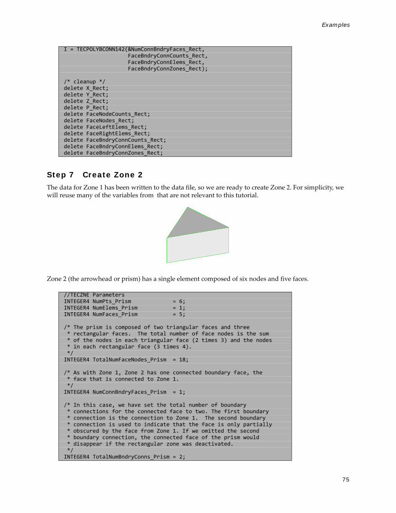
75
Examples
Step 7 Create Zone 2The data for Zone 1 has been written to the data file, so we are ready to create Zone 2. For simplicity, we will reuse many of the variables from that are not relevant to this tutorial.
Zone 2 (the arrowhead or prism) has a single element composed of six nodes and five faces.
I = TECPOLYBCONN142(&NumConnBndryFaces_Rect, FaceBndryConnCounts_Rect, FaceBndryConnElems_Rect, FaceBndryConnZones_Rect);
/* cleanup */delete X_Rect;delete Y_Rect;delete Z_Rect;delete P_Rect;delete FaceNodeCounts_Rect;delete FaceNodes_Rect;delete FaceLeftElems_Rect;delete FaceRightElems_Rect;delete FaceBndryConnCounts_Rect;delete FaceBndryConnElems_Rect;delete FaceBndryConnZones_Rect;
//TECZNE ParametersINTEGER4 NumPts_Prism = 6;INTEGER4 NumElems_Prism = 1;INTEGER4 NumFaces_Prism = 5;
/* The prism is composed of two triangular faces and three * rectangular faces. The total number of face nodes is the sum * of the nodes in each triangular face (2 times 3) and the nodes * in each rectangular face (3 times 4). */INTEGER4 TotalNumFaceNodes_Prism = 18;
/* As with Zone 1, Zone 2 has one connected boundary face, the * face that is connected to Zone 1. */INTEGER4 NumConnBndryFaces_Prism = 1;
/* In this case, we have set the total number of boundary * connections for the connected face to two. The first boundary * connection is the connection to Zone 1. The second boundary * connection is used to indicate that the face is only partially * obscured by the face from Zone 1. If we omitted the second * boundary connection, the connected face of the prism would * disappear if the rectangular zone was deactivated. */INTEGER4 TotalNumBndryConns_Prism = 2;

76
Step 8 Specify the variable values for Zone 2Now that the zone has been created, we must write the variable values to the file by calling TECDAT. While there are more elegant ways to define the grid coordinates for the prism, the values are defined explicitly in order to keep the example relatively simple.
Using the picture below, define the variable values.
I = TECZNE142((char*)”Zone 2: Prism”, &ZoneType, &NumPts_Prism, &NumElems_Prism, &NumFaces_Prism, &ICellMax, &JCellMax, &KCellMax, &SolutionTime, &StrandID, &ParentZone, &IsBlock, &NumFaceConnections, &FaceNeighborMode, &TotalNumFaceNodes_Prism, &NumConnBndryFaces_Prism, &TotalNumBndryConns_Prism, NULL, ValueLocation, NULL, &SharConn);
double *X_Prism = new double[NumPts_Prism];double *Y_Prism = new double[NumPts_Prism];double *Z_Prism = new double[NumPts_Prism];
/* Set the X and Y variable values, one z-plane at a time */double ZVal = 0;for (INTEGER4 ii = 0; ii < 2; ii++){ // triangle in Z=ZVal plane X_Prism[3*ii] = 3; Y_Prism[3*ii] = 4; Z_Prism[3*ii] = ZVal;
X_Prism[3*ii+1] = 7; Y_Prism[3*ii+1] = 2;

77
Examples
Step 9 Define the face map for the arrowheadBefore creating the data set, we have defined the node numbers, face numbers and element numbers. Using the following figure, specify the nodes that define each face.
Figure 3-4. The arrowhead with three faces visible (Face 2, Face 3 and Face 5). The remaining rectangular face is Face 1, and the remaining triangular face is Face 4).
The faces are created from the data file format using the FaceNodeCounts and FaceNodes array. The FaceNodeCounts array specifies the number of nodes contained in each face. The first value in the array is the number of nodes in Face 1, followed by the number of nodes in Face 2, and so forth. The FaceNodes array lists the node numbers in each face. The FaceNodes array first lists all of the nodes in Face 1, followed by all of the nodes in Face 2, and so forth.
In this example, Face 1 is composed of four nodes (Node 1, Node 3, Node 6 and Node 4). As such, the first value in the FaceNodeCounts array is “4” and the first four values in the FaceNodes array are [1, 3, 6, 4].
Z_Prism[3*ii+1] = ZVal;
X_Prism[3*ii+2] = 3; Y_Prism[3*ii+2] = 0; Z_Prism[3*ii+2] = ZVal;
ZVal = ZVal - 2;}
/* When we called TecZne, we specified that the variable 4 * (pressure) is cell-centered. As such, only NumElements number * of values needs to be written to the data file for the pressure * variable. */double *P_Prism = new double[NumElems_Prism];P_Prism[0] = 20;
I = TECDAT142(&NumPts_Prism, X_Prism, &IsDouble);I = TECDAT142(&NumPts_Prism, Y_Prism, &IsDouble);I = TECDAT142(&NumPts_Prism, Z_Prism, &IsDouble);I = TECDAT142(&NumElems_Prism, P_Prism, &IsDouble);
INTEGER4 *FaceNodeCounts_Prism = new INTEGER4[NumFaces_Prism];INTEGER4 *FaceNodes_Prism = new INTEGER4[TotalNumFaceNodes_Prism];
/* Because of the way we chose to number our faces, the first * three faces are rectangular and the last two are triangular. * The numbering of the faces is arbitrary, but the faces must * be referred to consistently. */

78
Step 10 Specify the neighboring elements for Zone 2Now that we have defined the nodes that compose each face, we must specify the element on either side of each face. The neighboring elements can be determined using the right-hand rule. For each face, place your right-hand along the face with your fingers pointing the direction of incrementing node numbers (i.e. from Node 1 to Node 2). The right side of your hand will indicate the right element, and the left side of your hand will indicate the left element. Refer to Section 3 - 8.3 “FaceRightElems and FaceLeftElems” for details.
The number zero is used to indicate that there isn't an element on that side of the face. A negative number is used when the neighboring element is in another zone. The value of the negative number points to the position in the FaceBoundaryConnectionElems and FaceBoundaryConnectionZones arrays that defines the element and zone numbers of the neighboring element. Refer to Step 11 for details.
Because of the way we numbered the nodes and faces, the right element for every face (except the face connected to the rectangular solid) is the element itself (Element 1) and the left element is "no-neighboring element" (Element 0).
for (INTEGER4 ii = 0; ii < 3; ii++) FaceNodeCounts_Prism[ii] = 4;
for (INTEGER4 ii = 3; ii < NumFaces_Prism; ii++) FaceNodeCounts_Prism[ii] = 3;
//Nodes for Face 1FaceNodes_Prism[0] = 1;FaceNodes_Prism[1] = 3;FaceNodes_Prism[2] = 6;FaceNodes_Prism[3] = 4;
//Nodes for Face 2FaceNodes_Prism[4] = 1;FaceNodes_Prism[5] = 4;FaceNodes_Prism[6] = 5;FaceNodes_Prism[7] = 2;
//Nodes for Face 3FaceNodes_Prism[8] = 3;FaceNodes_Prism[9] = 2;FaceNodes_Prism[10] = 5;FaceNodes_Prism[11] = 6;
//Nodes for Face 4FaceNodes_Prism[12] = 5;FaceNodes_Prism[13] = 4;FaceNodes_Prism[14] = 6;
//Nodes for Face 5FaceNodes_Prism[15] = 1;FaceNodes_Prism[16] = 2;FaceNodes_Prism[17] = 3;
/* Since this zone has just one element, all leftelems are * NoNeighboring Element and all right elems are itself. */INTEGER4 *FaceLeftElems_Prism = new INTEGER4[NumFaces_Prism];INTEGER4 *FaceRightElems_Prism = new INTEGER4[NumFaces_Prism];
for (INTEGER4 ii = 0; ii < NumFaces_Prism; ii++){ FaceRightElems_Prism[ii] = 1;

79
Examples
Step 11 Specify boundary connections for Zone 2The last step for creating Zone 2 is to specify the boundary connections.
FaceLeftElems_Prism[ii] = 0;}
/* The negative value in the FaceLeftElems array indicates that * the face is connected to an element in another zone. In this * case, Face 1 is connected to a face in Zone 1 (as indicated in * Line 6). The FaceBoundaryConnectionElems array lists all of * the element numbers in other zones that the current zone shares * boundary connections with. Similarly, the * FaceBoundaryConnectionZones array lists all of the zone numbers * with which the current zone shares boundaries. A negative * value in the FaceLeftElems or FaceRightElems array indicates * the position within these arrays that defines the neighboring * element and zone for a face. */FaceLeftElems_Prism[0] = -1;
I = TECPOLYFACE142(&NumFaces_Prism, FaceNodeCounts_Prism, FaceNodes_Prism, FaceLeftElems_Prism, FaceRightElems_Prism);
INTEGER4 *FaceBndryConnCounts_Prism = new INTEGER4[NumConnBndryFaces_Prism];FaceBndryConnCounts_Prism[0] = 2;
INTEGER4 *FaceBndryConnElems_Prism = new INTEGER4[TotalNumBndryConns_Prism];INTEGER4 *FaceBndryConnZones_Prism = new INTEGER4[TotalNumBndryConns_Prism];
/* As previously mentioned, a connected boundary face is a face * that has either multiple neighboring faces or neighbor(s) that * belong to another zone. Those cases are sufficient when the * combination of all of the face 痴 neighbors completely cover the * face. However, there are some cases (such as the bottom of the * arrowhead) where the face is not completely covered by its * neighbors. In those cases the face is referred to as 菟 artially * obscured ? A partially obscured face is indicated by * incrementing the value in TotalNumConnectedBoundaryFaces and * entering a value of 0 in both the FaceBndryConnectionElems and * FaceBoundaryConnectionZones arrays for the boundary connection * for the partially obscured face. */FaceBndryConnElems_Prism[0] = 0;FaceBndryConnZones_Prism[0] = 0;
/* Indicates that Face 1 is connected to Element 1 in Zone 1. */FaceBndryConnElems_Prism[1] = 1;FaceBndryConnZones_Prism[1] = 1;
I = TECPOLYBCONN142(&NumConnBndryFaces_Prism, FaceBndryConnCounts_Prism, FaceBndryConnElems_Prism, FaceBndryConnZones_Prism);
/* cleanup */delete X_Prism;
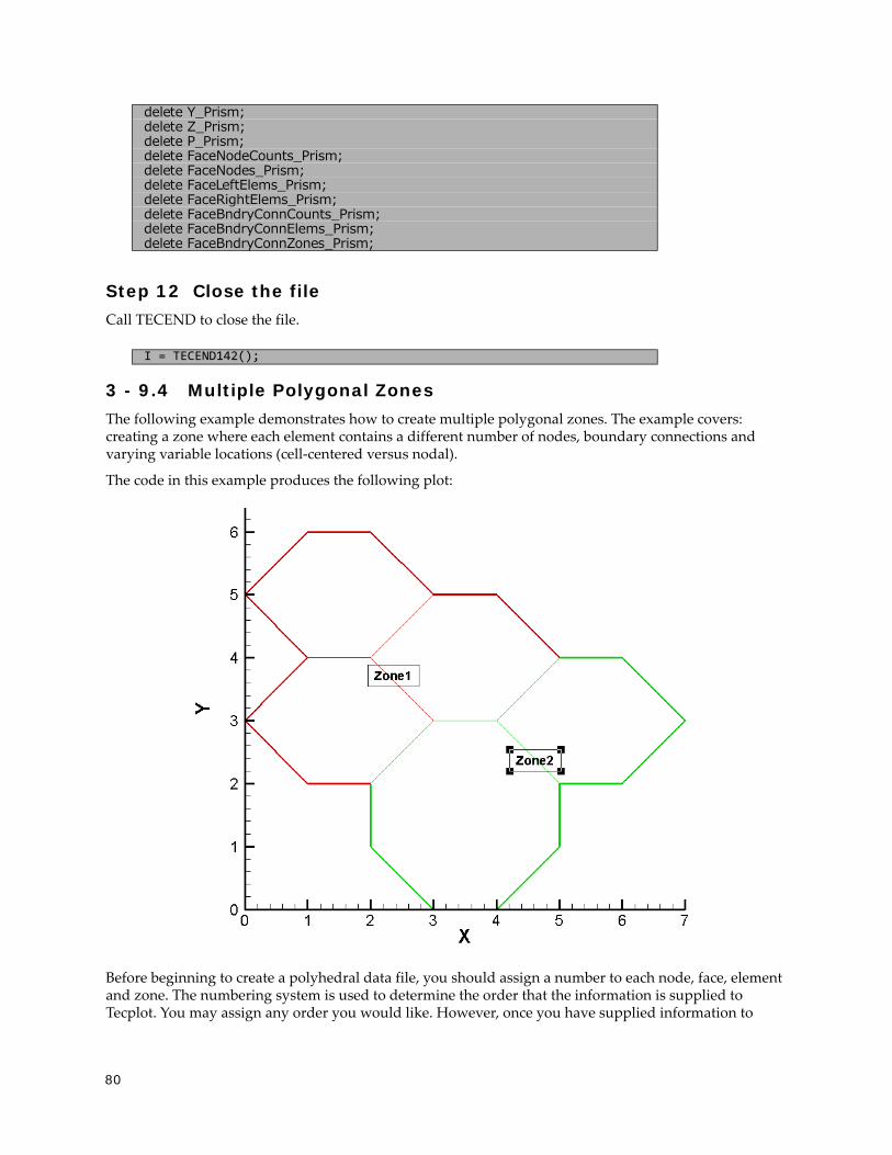
80
Step 12 Close the fileCall TECEND to close the file.
3 - 9.4 Multiple Polygonal ZonesThe following example demonstrates how to create multiple polygonal zones. The example covers: creating a zone where each element contains a different number of nodes, boundary connections and varying variable locations (cell-centered versus nodal).
The code in this example produces the following plot:
Before beginning to create a polyhedral data file, you should assign a number to each node, face, element and zone. The numbering system is used to determine the order that the information is supplied to Tecplot. You may assign any order you would like. However, once you have supplied information to
delete Y_Prism;delete Z_Prism;delete P_Prism;delete FaceNodeCounts_Prism;delete FaceNodes_Prism;delete FaceLeftElems_Prism;delete FaceRightElems_Prism;delete FaceBndryConnCounts_Prism;delete FaceBndryConnElems_Prism;delete FaceBndryConnZones_Prism;
I = TECEND142();

81
Examples
Tecplot, you cannot change the number configuration. For this example, we have selected the numbering system shown below:
Zone 1 has a total of three elements, thirteen unique nodes and fifteen faces. Zone 2 has two elements, twelve nodes and thirteen faces.
In order to keep the example as simple as possible, error checking is not included. If you plan to compile this example, be sure to include: TECIO.h.
For complete details on the parameters used and the function syntax for each TecIO function, refer to Section 3 - 7 “Binary Data File Function Reference”. When creating a binary data file using the TecIO library, the functions must be called in a specific order. Refer to Section 3 - 4 “Binary Data File Function Calling Sequence” for details.
Step 1 Initialize the Data FileThe first step for creating a binary data file using the TecIO library is to initialize and open the data file by calling TECINI
INTEGER4 I; /* use to check return values */
INTEGER4 Debug = 1;INTEGER4 VIsDouble = 0;INTEGER4 FileType = 0;INTEGER4 FileFormat = 0; // 0 == PLT, 1 == SZPLT
I = TECINI142((char*)”Example: Multiple polygonal zones”, (char*)”X Y P”, /* Defines the variables for the data file. * Each zone must contain each of the vars * listed here. The order of the variables * in the list is used to define the * variable number (e.g. X is Variable 1). * When referring to variables in other * TecIO functions, you will refer to the * variable by its number. */ (char*)”HexagonsAndOctagon.plt”, (char*)”.”, /* scratch directory */ &FileFormat, &FileType, &Debug, &VIsDouble);

82
Step 2 Create Zone 1 (3 Hexagons)The first step toward creating Zone 1 is to call TECZNE. TECZNE is used to initialize the zone and specify parameters that apply to the entire zone (e.g. number of nodes, number of elements and variable location).
/* TECZNE Parameters */INTEGER4 ZoneType = 6; /* FE Polygon */INTEGER4 NumPts_Z1 = 13; /* the number of unique * nodes in the zone. */INTEGER4 NumElems_Z1 = 3;INTEGER4 NumFaces_Z1 = 15; /* the number of unique * faces in the zone. */INTEGER4 ICellMax = 0; /* not used */INTEGER4 JCellMax = 0; /* not used */INTEGER4 KCellMax = 0; /* not used */double SolutionTime = 0.0;INTEGER4 StrandID = 0;INTEGER4 ParentZone = 0;INTEGER4 IsBlock = 1;INTEGER4 NumFaceConnections = 0;INTEGER4 FaceNeighborMode = 1;INTEGER4 SharConn = 0;
INTEGER4 ValueLocation[3] = { 1, 1, 0 };
/* For a polygonal zone, the total number of face nodes is * twice the total number of faces. This is because each face * is composed of exactly two nodes. */INTEGER4 TotalNumFaceNodes_Z1 = 2 * NumFaces_Z1;
/* A boundary face is a face that is neighbored by an element

83
Examples
Step 3 Specify the variable values for Zone 1The variable values are written to the data file via the TECDAT function. For each variable you must provide either a total number of values equivalent to NumPts (if the variables are nodal) or a total number of values equivalent to NumElements (if the variables are cell-centered). The variable location is specified by the VarLocation parameter in TECZNE. In this example, X and Y are nodal variables and P is cell-centered.
The order in which the variable values must be provided is established by the numbering scheme (specified at the beginning of the example). The first value for each nodal variable (X and Y) corresponds to Node 1, the second value corresponds to Node 2 and so forth. The first value for the cell-centered value is for Element 1, the second value is for the second element or cell and so forth.
* or elements in another zone or zone(s). In Zone 1, Face 9, * Face 10 and Face 12 have a neighbor in Zone 2. Therefore, * the total number of boundary faces is ?? */INTEGER4 TotalNumBndryFaces_Z1 = 3;
/* Each boundary face has one or more boundary connections. A * boundary connection is defined as another element in another * zone. Face 9 has a boundary connection with Element 1 in * Zone 2. In this example, each boundary face is connected to * one other element, so the total number of boundary * connections is equivalent to the total number of boundary * faces (3). */INTEGER4 TotalNumBndryConns_Z1 = 3;
I = TECZNE142((char*)"Zone 1: 3 Hexagons", /* Specifies the name of * the entire dataset. When * the file is loaded into * Tecplot, the value is * available via the Data * Set Info dialog. */ &ZoneType, &NumPts_Z1, &NumElems_Z1, &NumFaces_Z1, &ICellMax, &JCellMax, &KCellMax, &SolutionTime, &StrandID, &ParentZone, &IsBlock, &NumFaceConnections, &FaceNeighborMode, &TotalNumFaceNodes_Z1, &TotalNumBndryFaces_Z1, &TotalNumBndryConns_Z1, NULL, ValueLocation, NULL, &SharConn);

84
In order for the example to be easily followed, the grid coordinates are explicitly defined. When working with larger data sets, you will likely wish to use equations to define your coordinates. Refer to the picture in Step 2 for the X and Y coordinate values for Zone 1.
/* TECDAT Parameters */double *X_Z1 = new double[NumPts_Z1];double *Y_Z1 = new double[NumPts_Z1];
X_Z1[0] = 1;Y_Z1[0] = 6;
X_Z1[1] = 2;Y_Z1[1] = 6;
X_Z1[2] = 3;Y_Z1[2] = 5;
X_Z1[3] = 2;Y_Z1[3] = 4;
X_Z1[4] = 1;Y_Z1[4] = 4;
X_Z1[5] = 0;Y_Z1[5] = 5;
X_Z1[6] = 4;Y_Z1[6] = 5;
X_Z1[7] = 5;Y_Z1[7] = 4;
X_Z1[8] = 4;Y_Z1[8] = 3;
X_Z1[9] = 3;Y_Z1[9] = 3;
X_Z1[10] = 2;Y_Z1[10] = 2;
X_Z1[11] = 1;Y_Z1[11] = 2;
X_Z1[12] = 0;Y_Z1[12] = 3;
double *P_Z1 = new double[NumElems_Z1];P_Z1[0] = 2;P_Z1[1] = 4;P_Z1[2] = 5;
INTEGER4 IsDouble = 1;I = TECDAT142(&NumPts_Z1, X_Z1, &IsDouble);I = TECDAT142(&NumPts_Z1, Y_Z1, &IsDouble);I = TECDAT142(&NumElems_Z1, P_Z1, &IsDouble);delete X_Z1;delete Y_Z1;delete P_Z1;

85
Examples
Step 4 Specify the face map data for Zone 1Use the picture in Step 2 to specify the nodes that compose each face. The first two values in the face node array define Face 1, the next two define Face 2, and so on.
/* TecPolyFace Parameters */
/* Create a FaceNodes array, dimensioned by the total number * of face nodes in the zone. */INTEGER4 *FaceNodes_Z1 = new INTEGER4[TotalNumFaceNodes_Z1];
/* Face Nodes for Element 1 */FaceNodes_Z1[0] = 1;FaceNodes_Z1[1] = 2;
FaceNodes_Z1[2] = 2;FaceNodes_Z1[3] = 3;
FaceNodes_Z1[4] = 3;FaceNodes_Z1[5] = 4;
FaceNodes_Z1[6] = 4;FaceNodes_Z1[7] = 5;
FaceNodes_Z1[8] = 5;FaceNodes_Z1[9] = 6;
FaceNodes_Z1[10] = 6;FaceNodes_Z1[11] = 1;
/* Face Nodes for Element 2 */FaceNodes_Z1[12] = 3;FaceNodes_Z1[13] = 7;
FaceNodes_Z1[14] = 7;FaceNodes_Z1[15] = 8;
FaceNodes_Z1[16] = 8;FaceNodes_Z1[17] = 9;
FaceNodes_Z1[18] = 9;FaceNodes_Z1[19] = 10;
FaceNodes_Z1[20] = 10;FaceNodes_Z1[21] = 4;
/* Face Nodes for Element 3 */FaceNodes_Z1[22] = 10;FaceNodes_Z1[23] = 11;
FaceNodes_Z1[24] = 11;FaceNodes_Z1[25] = 12;
FaceNodes_Z1[26] = 12;FaceNodes_Z1[27] = 13;
FaceNodes_Z1[28] = 13;FaceNodes_Z1[29] = 5;

86
Step 5 Specify the neighboring elements for Zone 1Now that we have defined the nodes that compose each face, we must specify the element on either side of each face. The neighboring elements can be determined using the right-hand rule. For each face, place your right-hand along the face with your fingers pointing the direction of incrementing node numbers (i.e. from Node 1 to Node 2). The right side of your hand will indicate the right element, and the left side of your hand will indicate the left element. Refer to Section 3 - 8.3 “FaceRightElems and FaceLeftElems” for details.
The number zero is used to indicate that there isn't an element on that side of the face. A negative number is used when the neighboring element is in another zone. The value of the negative number points to the position in the FaceBoundaryConnectionElems and FaceBoundaryConnectionZones arrays that defines the element and zone numbers of the neighboring element. Refer to Step 6 for details.
Because of the way we numbered the nodes and faces, the right element for every face is the element itself. The left element will either be: another element in the zone, “no neighboring element”, or an element in Zone 2. The term “no neighboring element” is used to describe a face that is on the edge of the entire data set (not just the zone).
INTEGER4 *FaceLeftElems_Z1 = new INTEGER4[NumFaces_Z1];INTEGER4 *FaceRightElems_Z1 = new INTEGER4[NumFaces_Z1];
/* Left Face Elems for Element 1 */FaceLeftElems_Z1[0] = 0;FaceLeftElems_Z1[1] = 0;FaceLeftElems_Z1[2] = 2;FaceLeftElems_Z1[3] = 3;FaceLeftElems_Z1[4] = 0;
/* Left Face Elems for Element 2 */FaceLeftElems_Z1[5] = 0;FaceLeftElems_Z1[6] = 0;FaceLeftElems_Z1[7] = 0;FaceLeftElems_Z1[8] = -1;FaceLeftElems_Z1[9] = -2;FaceLeftElems_Z1[10] = 3;
/* Left Face Elems for Element 3 */FaceLeftElems_Z1[11] = -3;FaceLeftElems_Z1[12] = 0;FaceLeftElems_Z1[13] = 0;FaceLeftElems_Z1[14] = 0;
/* Set Right Face Elems. Because of the way we numbered the * nodes and faces, the right element for every face is the * element itself. */for (INTEGER4 ii = 0; ii < 6; ii++) FaceRightElems_Z1[ii] = 1;
for (INTEGER4 ii = 6; ii < 11; ii++) FaceRightElems_Z1[ii] = 2;
for (INTEGER4 ii = 11; ii <= 14; ii++) FaceRightElems_Z1[ii] = 3;
I = TECPOLYFACE142(&NumFaces_Z1, NULL, /* Not used for polygon zones */ FaceNodes_Z1, FaceLeftElems_Z1, FaceRightElems_Z1);
87
Examples
Step 6 Specify the boundary connections for Zone 1The final step for creating Zone 1 is to define the boundary connections.
delete FaceNodes_Z1;delete FaceLeftElems_Z1;delete FaceRightElems_Z1;
/* TecPolyBConn Parameters */
/* The FaceBndryConnectionCounts array is used to define the * number of boundary connections for each face that has a * boundary connection. For example, if a zone has three * boundary connections in total (NumConnectedBoundaryFaces), * two of those boundary connections are in one face, and the * remaining boundary connection is in a second face, the * FaceBndryConnectionCounts array would be: [2 1]. * * In this example, the total number of connected boundary * faces (specified via TECZNE) is equal to three. Each * boundary face is connected to only one other element, * so the FaceBoundaryConnectionCounts array is (1, 1, 1). */INTEGER4 FaceBndryConnectionCounts_Z1[3] = {1, 1, 1};
/* The value(s) in the FaceBndryConnectionElems and * FaceBndryConnectionZones arrays specifies the element number * and zone number, respectively, that a given boundary * connection is connected to. In this case, the first * boundary connection face is connected to Element 1 in Zone 2 * and the remaining connection is to Element 2 in Zone 2. */INTEGER4 FaceBndryConnectionElems_Z1[3] = {1, 2, 2};INTEGER4 FaceBndryConnectionZones_Z1[3] = {2, 2, 2};
I = TECPOLYBCONN142(&TotalNumBndryFaces_Z1, FaceBndryConnectionCounts_Z1, FaceBndryConnectionElems_Z1, FaceBndryConnectionZones_Z1);

88
Step 7 Create Zone 2Now that Zone 1 is complete, we are ready to begin creating Zone 2 by calling TECZNE. For simplicity, we are reusing many of the variables that were defined for Zone 1.
INTEGER4 NumPts_Z2 = 12; /* number of unique * nodes in the zone */INTEGER4 NumElems_Z2 = 2;INTEGER4 NumFaces_Z2 = 13; /* number of unique * faces in the zone */INTEGER4 NumFaceConnections_Z2 = 0;/* In polygonal zones, each face has exactly two nodes */INTEGER4 TotalNumFaceNodes_Z2 = NumFaces_Z2 * 2;
/* A boundary face is a face that is neighbored by an element or * elements from another zone or zone(s). In Zone 2, Face 6, * Face 7 and Face 13 have a neighbor in Zone 1. Therefore, the * total number of boundary faces is ?? */INTEGER4 TotalNumBndryFaces_Z2 = 3;
/* Each boundary face has one or more boundary connections. In * this example, each boundary face is connected to one other * element (i.e. the number of boundary faces and the number of * boundary connections is one-to-one). */INTEGER4 TotalNumBndryConns_Z2 = 3;
I = TECZNE142((char*)"Zone 2: 1 Hexagon and 1 Octagon", &ZoneType, &NumPts_Z2, &NumElems_Z2, &NumFaces_Z2, &ICellMax, &JCellMax, &KCellMax, &SolutionTime, &StrandID,

89
Examples
Step 8 Specify the variable values for Zone 2The variable values are written to the data file via the TECDAT function. For each variable you must provide either a total number of values equivalent to NumPts (if the variables are nodal) or equivalent to NumElements (if the variables are cell-centered). The variable location is specified by the VarLocation parameter in TECZNE. In this example, X and Y are nodal variables and P is cell-centered.
The order in which the variable values must be provided is established by the numbering scheme specified at the beginning of the example. The first value for each nodal variable (X and Y) corresponds to Node 1, the second value corresponds to Node 2 and so forth. The first value for the cell-centered value is for Element 1, the second value is for the second element or cell and so forth.
In order for the example to be easily followed, the grid coordinates are explicitly defined. When working with larger data sets, you will likely wish to use equations to define your coordinates. Refer to the picture in Step 7 for the X and Y coordinate values for Zone 2.
&ParentZone, &IsBlock, &NumFaceConnections_Z2, &FaceNeighborMode, &TotalNumFaceNodes_Z2, &TotalNumBndryFaces_Z2, &TotalNumBndryConns_Z2, NULL, ValueLocation, NULL, &SharConn);
double *X_Z2 = new double[NumPts_Z2];double *Y_Z2 = new double[NumPts_Z2];
X_Z2[0] = 5;Y_Z2[0] = 4;
X_Z2[1] = 6;Y_Z2[1] = 4;
X_Z2[2] = 7;Y_Z2[2] = 3;
X_Z2[3] = 6;Y_Z2[3] = 2;
X_Z2[4] = 5;Y_Z2[4] = 2;
X_Z2[5] = 4;Y_Z2[5] = 3;
X_Z2[6] = 3;Y_Z2[6] = 3;
X_Z2[7] = 5;Y_Z2[7] = 1;
X_Z2[8] = 4;Y_Z2[8] = 0;
X_Z2[9] = 3;Y_Z2[9] = 0;

90
Step 9 Specify the face map for Zone 2Use the picture in Step 7 to specify which nodes compose which face. The first two values in the face node array define Face 1, the next two define Face 2, and so on.
X_Z2[10] = 2;Y_Z2[10] = 1;
X_Z2[11] = 2;Y_Z2[11] = 2;
/* In the call to TecZne, P was set to a cell centered variable. * As such, only two values need to be defined. */double *P_Z2 = new double[NumPts_Z2];
P_Z2[0] = 8;P_Z2[1] = 6;
I = TECDAT142(&NumPts_Z2, X_Z2, &IsDouble);I = TECDAT142(&NumPts_Z2, Y_Z2, &IsDouble);I = TECDAT142(&NumElems_Z2, P_Z2, &IsDouble);
delete X_Z2;delete Y_Z2;delete P_Z2;
INTEGER4 *FaceNodes_Z2;FaceNodes_Z2 = new INTEGER4[TotalNumFaceNodes_Z2];
/* Face Nodes for Element 1 */FaceNodes_Z2[0] = 1;FaceNodes_Z2[1] = 2;
FaceNodes_Z2[2] = 2;FaceNodes_Z2[3] = 3;
FaceNodes_Z2[4] = 3;FaceNodes_Z2[5] = 4;
FaceNodes_Z2[6] = 4;FaceNodes_Z2[7] = 5;
FaceNodes_Z2[8] = 5;FaceNodes_Z2[9] = 6;
FaceNodes_Z2[10] = 6;FaceNodes_Z2[11] = 1;
/* Face Nodes for Element 2 */FaceNodes_Z2[12] = 7;FaceNodes_Z2[13] = 6;
FaceNodes_Z2[14] = 5;FaceNodes_Z2[15] = 8;
FaceNodes_Z2[16] = 8;FaceNodes_Z2[17] = 9;
FaceNodes_Z2[18] = 9;FaceNodes_Z2[19] = 10;
91
Examples
Step 10 Specify the neighboring elements for Zone 2Now that we have defined the nodes that compose each face, we must specify the element on either side of each face. The neighboring elements can be determined using the right-hand rule. For each face, place your right-hand along the face with your fingers pointing the direction of incrementing node numbers (i.e. from Node 1 to Node 2). The right side of your hand will indicate the right element, and the left side of your hand will indicate the left element. Refer to Section 3 - 8.3 “FaceRightElems and FaceLeftElems” for details.
The number zero is used to indicate that there isn't an element on that side of the face. A negative number is used when the neighboring element is in another zone. The value of the negative number points to the position in the FaceBoundaryConnectionElems and FaceBoundaryConnectionZones arrays that defines the element and zone numbers of the neighboring element. Refer to Step 11 for details.
Because of the way we numbered the nodes and faces, the right element for every face is the element itself. The left element will either be: another element in the zone, “no neighboring element”, or an element in Zone 2. The term “no neighboring element” is used to describe a face that is on the edge of the entire data set (not just the zone).
FaceNodes_Z2[20] = 10;FaceNodes_Z2[21] = 11;
FaceNodes_Z2[22] = 11;FaceNodes_Z2[23] = 12;
FaceNodes_Z2[24] = 12;FaceNodes_Z2[25] = 7;
/* Specify the right and left neighboring elements. * The neighboring elements can be determined using the * right-hand rule. For each face, place your right-hand along * the face with your fingers pointing the direction of * incrementing node numbers (i.e. from Node 1 to Node 2). The * right side of your hand will indicate the right element, * and the left side of your hand will indicate the left * element. A value of zero indicates that there is no * neighboring element on that side. A negative value * indicates that the neighboring element is in another zone. * The number is a pointer into the FaceBndryConnectionElems * and FaceBndryConnectionZones arrays. */
INTEGER4 *FaceLeftElems_Z2 = new INTEGER4[NumFaces_Z2];INTEGER4 *FaceRightElems_Z2 = new INTEGER4[NumFaces_Z2];
/* Left Face Elems for Element 1 */FaceLeftElems_Z2[0] = 0;FaceLeftElems_Z2[1] = 0;FaceLeftElems_Z2[2] = 0;FaceLeftElems_Z2[3] = 0;FaceLeftElems_Z2[4] = 2;FaceLeftElems_Z2[5] = -1;
/* Left Face Elems for Element 2 */FaceLeftElems_Z2[6] = -2;FaceLeftElems_Z2[7] = 0;FaceLeftElems_Z2[8] = 0;FaceLeftElems_Z2[9] = 0;FaceLeftElems_Z2[10] = 0;FaceLeftElems_Z2[11] = 0;FaceLeftElems_Z2[12] = -3;

92
Step 11 Specify the Boundary Connections for Zone 2The final step for creating Zone 2 is to define the boundary connections
Step 12 Close the file using TECENDCall TECEND to close the file.
/* Set Right Face Elems. Because of the way we numbered the * nodes and faces, the right element for every face is the * element itself. */for (INTEGER4 ii = 0; ii < 6; ii++) FaceRightElems_Z2[ii] = 1;
for (INTEGER4 ii = 6; ii < 13; ii++) FaceRightElems_Z2[ii] = 2;
I = TECPOLYFACE142(&NumFaces_Z2, NULL, FaceNodes_Z2, FaceLeftElems_Z2, FaceRightElems_Z2);
delete FaceNodes_Z2;delete FaceLeftElems_Z2;delete FaceRightElems_Z2;
/* The FaceBndryConnectionCounts array is used to define the * number of boundary connections for each face that has a * boundary connection. In this example, the total number of * connected boundary faces (specified via TECZNE) is equal to * three. Each boundary face is connected to only one other * element, so the FaceBoundaryConnectionCounts array is * (1, 1, 1). */INTEGER4 FaceBndryConnectionCounts_Z2[3] = {1, 1, 1};
/* The value(s) in the FaceBndryConnectionElems and * FaceBndryConnectionZones arrays specifies that element * number and zone number, respectively, that a given boundary * connection is connected to. In this case, the first boundary * connection face is connected to Element 2 in Zone 1 and the * remaining connections are Element 3 in Zone 1. */INTEGER4 FaceBndryConnectionElems_Z2[3] = {2, 3, 3};INTEGER4 FaceBndryConnectionZones_Z2[3] = {1, 1, 1};
I = TECPOLYBCONN142(&TotalNumBndryFaces_Z2, FaceBndryConnectionCounts_Z2, FaceBndryConnectionElems_Z2, FaceBndryConnectionZones_Z2);
I = TECEND142();

93
Examples
3 - 9.5 Polyhedral ExampleThe following example (written in C) illustrates how to create a single polyhedral cell using the TecIO library.
#include “TECIO.h”#include “MASTER.h” /* for defintion of NULL */
int main(){ /* Call TECINI142 */ INTEGER4 FileType = 0; /* 0 for full file */ INTEGER4 FileFormat = 0; // 0 == PLT, 1 == SZPLT; Only PLT is currently // supported for polyhedral zones INTEGER4 Debug = 0; INTEGER4 VIsDouble = 1; INTEGER4 I = 0; /* use to check return codes */
I = TECINI142((char*)”Pyramid”, /* Data Set Title */ (char*)”X Y Z”, /* Variable List */ (char*)”pyramid.plt”, /* File Name */ (char*)”.”, /* Scratch Directory */ &FileFormat, &(FileType), &(Debug), &(VIsDouble));
/* Call TECZNE142 */ INTEGER4 ZoneType = 7; /* 7 for FEPolyhedron */ INTEGER4 NumNodes = 5; /* number of unique nodes */ INTEGER4 NumElems = 1; /* number of elements */ INTEGER4 NumFaces = 5; /* number of unique faces */
INTEGER4 ICellMax = 0; /* Not Used, set to zero */ INTEGER4 JCellMax = 0; /* Not Used, set to zero */ INTEGER4 KCellMax = 0; /* Not Used, set to zero */
double SolTime = 12.65; /* solution time */ INTEGER4 StrandID = 0; /* static zone */ INTEGER4 ParentZone = 0; /* no parent zone */
INTEGER4 IsBlock = 1; /* block format */
INTEGER4 NFConns = 0; /* not used for FEPolyhedron * zones */ INTEGER4 FNMode = 0; /* not used for FEPolyhedron * zones */
INTEGER4 *PassiveVarArray = NULL; INTEGER4 *ValueLocArray = NULL; INTEGER4 *VarShareArray = NULL;
INTEGER4 ShrConn = 0;
/* The number of face nodes in the zone. This example creates * a zone with a single pyramidal cell. This cell has four * triangular faces and one rectangular face, yielding a total * of 16 face nodes. */ INTEGER4 NumFaceNodes = 16; INTEGER4 NumBConns = 0; /* No Boundary Connections */

94
INTEGER4 NumBItems = 0; /* No Boundary Items */
I = TECZNE142((char*)”Polyhedral Zone (Octahedron)”, &ZoneType, &NumNodes, &NumElems, &NumFaces, &ICellMax, &JCellMax, &KCellMax, &SolTime, &StrandID, &ParentZone, &IsBlock, &NFConns, &FNMode, &NumFaceNodes, &NumBConns, &NumBItems, PassiveVarArray, ValueLocArray, VarShareArray, &ShrConn);
/* Initialize arrays of nodal data */ double *X = new double[NumNodes]; double *Y = new double[NumNodes]; double *Z = new double[NumNodes];
X[0] = 0; Y[0] = 0; Z[0] = 0;
X[1] = 1; Y[1] = 1; Z[1] = 2;
X[2] = 2; Y[2] = 0; Z[2] = 0;
X[3] = 2; Y[3] = 2; Z[3] = 0;
X[4] = 0; Y[4] = 2; Z[4] = 0;
/* Write the data (using TECDAT142) */ INTEGER4 DIsDouble = 1; /* One for double precision */ I = TECDAT142(&NumNodes, X, &DIsDouble); I = TECDAT142(&NumNodes, Y, &DIsDouble); I = TECDAT142(&NumNodes, Z, &DIsDouble);
delete X; delete Y; delete Z;
/* Define the Face Nodes. * * The FaceNodes array is used to indicate which nodes define * which face. As mentioned earlier, the number of the nodes is * implicitly defined by the order in which the nodal data is
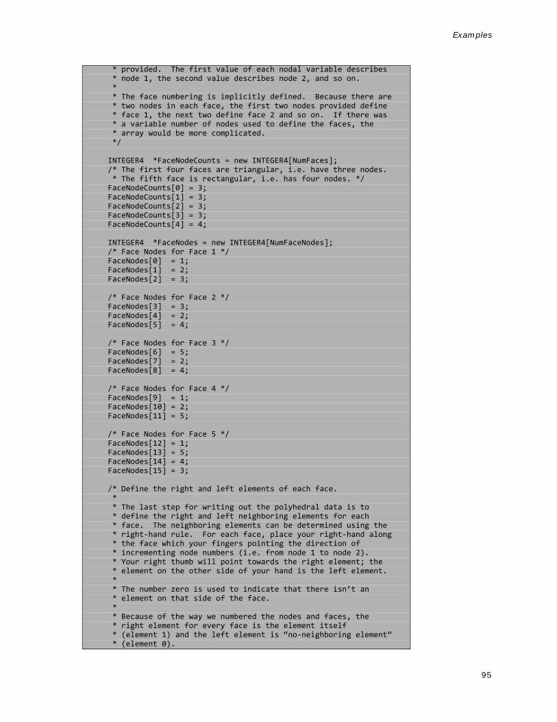
95
Examples
* provided. The first value of each nodal variable describes * node 1, the second value describes node 2, and so on. * * The face numbering is implicitly defined. Because there are * two nodes in each face, the first two nodes provided define * face 1, the next two define face 2 and so on. If there was * a variable number of nodes used to define the faces, the * array would be more complicated. */
INTEGER4 *FaceNodeCounts = new INTEGER4[NumFaces]; /* The first four faces are triangular, i.e. have three nodes. * The fifth face is rectangular, i.e. has four nodes. */ FaceNodeCounts[0] = 3; FaceNodeCounts[1] = 3; FaceNodeCounts[2] = 3; FaceNodeCounts[3] = 3; FaceNodeCounts[4] = 4;
INTEGER4 *FaceNodes = new INTEGER4[NumFaceNodes]; /* Face Nodes for Face 1 */ FaceNodes[0] = 1; FaceNodes[1] = 2; FaceNodes[2] = 3;
/* Face Nodes for Face 2 */ FaceNodes[3] = 3; FaceNodes[4] = 2; FaceNodes[5] = 4;
/* Face Nodes for Face 3 */ FaceNodes[6] = 5; FaceNodes[7] = 2; FaceNodes[8] = 4;
/* Face Nodes for Face 4 */ FaceNodes[9] = 1; FaceNodes[10] = 2; FaceNodes[11] = 5;
/* Face Nodes for Face 5 */ FaceNodes[12] = 1; FaceNodes[13] = 5; FaceNodes[14] = 4; FaceNodes[15] = 3;
/* Define the right and left elements of each face. * * The last step for writing out the polyhedral data is to * define the right and left neighboring elements for each * face. The neighboring elements can be determined using the * right-hand rule. For each face, place your right-hand along * the face which your fingers pointing the direction of * incrementing node numbers (i.e. from node 1 to node 2). * Your right thumb will point towards the right element; the * element on the other side of your hand is the left element. * * The number zero is used to indicate that there isn’t an * element on that side of the face. * * Because of the way we numbered the nodes and faces, the * right element for every face is the element itself * (element 1) and the left element is “no-neighboring element” * (element 0).

96
3 - 9.6 IJ-ordered zoneThe following example illustrates how to create a simple IJ-ordered zone. TECZNE142 is called first to initialize the zone.
*/
INTEGER4 *FaceLeftElems = new INTEGER4[NumFaces]; FaceLeftElems[0] = 1; FaceLeftElems[1] = 1; FaceLeftElems[2] = 0; FaceLeftElems[3] = 0; FaceLeftElems[4] = 0;
INTEGER4 *FaceRightElems = new INTEGER4[NumFaces]; FaceRightElems[0] = 0; FaceRightElems[1] = 0; FaceRightElems[2] = 1; FaceRightElems[3] = 1; FaceRightElems[4] = 1;
/* Write the face map (created above) using TECPOLYFACE142. */ I = TECPOLYFACE142(&NumFaces, FaceNodeCounts, /* The face node counts array */ FaceNodes, /* The face nodes array */ FaceLeftElems, /* The left elements array */ FaceRightElems); /* The right elements array */
delete FaceNodeCounts; delete FaceNodes; delete FaceLeftElems; delete FaceRightElems;
I = TECEND142(); return 0;}
#include “TECIO.h”#include “MASTER.h” /* for defintion of NULL */
int main(){ INTEGER4 Debug = 1; INTEGER4 VIsDouble = 0; INTEGER4 FileType = 0; INTEGER4 FileFormat = 0; // 0 == PLT, 1 == SZPLT INTEGER4 I = 0; /* Used to track return codes */
/* * Open the file and write the tecplot datafile * header information */ I = TECINI142((char*)”IJ Ordered Zones”, /* Name of the entire * dataset. */ (char*)”X Y P”, /* Defines the variables for the data * file. Each zone must contain each of * the variables listed here. The order * of the variables in the list is used * to define the variable number (e.g. * X is Var 1). */ (char*)”ij_ordered.plt”, (char*)”.”, /* Scratch Directory */

97
Examples
&FileFormat, &FileType, &Debug, &VIsDouble);
float X1[4]; float Y1[4]; float P1[4]; float X2[4]; float Y2[4]; float P2[4];
INTEGER4 ICellMax = 0; INTEGER4 JCellMax = 0; INTEGER4 KCellMax = 0; INTEGER4 DIsDouble = 0; double SolTime = 360.0; INTEGER4 StrandID = 0; /* StaticZone */ INTEGER4 ParentZn = 0; INTEGER4 IsBlock = 1; /* Block */ INTEGER4 NFConns = 0; INTEGER4 FNMode = 0; INTEGER4 TotalNumFaceNodes = 1; INTEGER4 TotalNumBndryFaces = 1; INTEGER4 TotalNumBndryConnections = 1; INTEGER4 ShrConn = 0;
/*Ordered Zone Parameters*/ INTEGER4 IMax = 2; INTEGER4 JMax = 2; INTEGER4 KMax = 1;
X1[0] = .125; Y1[0] = .5; P1[0] = 5;
X1[1] = .625; Y1[1] = .5; P1[1] = 7.5;
X1[2] = .125; Y1[2] = .875; P1[2] = 10;
X1[3] = .625; Y1[3] = .875; P1[3] = 7.5;
X2[0] = .375; Y2[0] = .125; P2[0] = 5;
X2[1] = .875; Y2[1] = .125; P2[1] = 7.5;
X2[2] = .375; Y2[2] = .5; P2[2] = 10;
X2[3] = .875; Y2[3] = .5; P2[3] = 7.5;
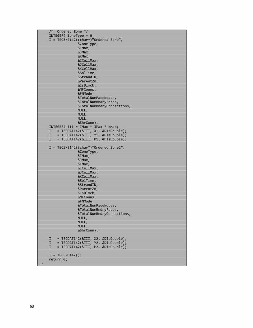
98
/* Ordered Zone */ INTEGER4 ZoneType = 0; I = TECZNE142((char*)”Ordered Zone”, &ZoneType, &IMax, &JMax, &KMax, &ICellMax, &JCellMax, &KCellMax, &SolTime, &StrandID, &ParentZn, &IsBlock, &NFConns, &FNMode, &TotalNumFaceNodes, &TotalNumBndryFaces, &TotalNumBndryConnections, NULL, NULL, NULL, &ShrConn); INTEGER4 III = IMax * JMax * KMax; I = TECDAT142(&III, X1, &DIsDouble); I = TECDAT142(&III, Y1, &DIsDouble); I = TECDAT142(&III, P1, &DIsDouble);
I = TECZNE142((char*)”Ordered Zone2”, &ZoneType, &IMax, &JMax, &KMax, &ICellMax, &JCellMax, &KCellMax, &SolTime, &StrandID, &ParentZn, &IsBlock, &NFConns, &FNMode, &TotalNumFaceNodes, &TotalNumBndryFaces, &TotalNumBndryConnections, NULL, NULL, NULL, &ShrConn);
I = TECDAT142(&III, X2, &DIsDouble); I = TECDAT142(&III, Y2, &DIsDouble); I = TECDAT142(&III, P2, &DIsDouble);
I = TECEND142(); return 0;}

99
Examples
3 - 9.7 Switching Between Two FilesIn this simplified example, information is written to two separate files. First, one file is created and a zone is written to the file. Then, a second file is created and a zone and auxiliary data are written to the file. The second file is closed and the auxiliary data is written to the first file.INTEGER4 DemoTecFil(void)
#include “TECIO.h”#include “MASTER.h” /* for defintion of NULL */#include <string.h>
int main(){ /* * Open the file and write the tecplot datafile * header information */ INTEGER4 Debug = 1; INTEGER4 VIsDouble = 0; INTEGER4 FileType = 0; INTEGER4 FileFormat = 0; // 0 == PLT, 1 == SZPLT INTEGER4 I = 0; /* Used to check the return value */
I = TECINI142((char*)”SIMPLE DATASET”, /* Name of the entire dataset.*/
(char*)”X1 Y1 P1”, /* Defines the variables for the data * file. Each zone must contain each of * the variables listed here. The order * of the variables in the list is used * to define the variable number (e.g. * X1 is Var 1). */ (char*)”file1.plt”, (char*)”.”, /* Scratch Directory */ &FileFormat, &FileType, &Debug, &VIsDouble);
/* Set the parameters for TecZne */ INTEGER4 ZoneType = 0; /* sets the zone type to * ordered */ INTEGER4 IMax = 2; /* Create an IJ-ordered zone, * by using IMax and JMax * values that are greater * than one, and setting KMax * to one. */ INTEGER4 JMax = 2; INTEGER4 KMax = 1;
double SolTime = 0; INTEGER4 StrandID = 0; /* StaticZone */ INTEGER4 ParentZn = 0; /* used for surface streams */
INTEGER4 ICellMax = 0; /* not used */ INTEGER4 JCellMax = 0; /* not used */ INTEGER4 KCellMax = 0; /* not used */

100
INTEGER4 IsBlock = 1; /* Block */
INTEGER4 NFConns = 0; /* this example does not use * face neighbors */ INTEGER4 FNMode = 0; INTEGER4 TotalNumFaceNodes = 1; INTEGER4 TotalNumBndryFaces = 1; INTEGER4 TotalNumBndryConn = 1; INTEGER4 ShrConn = 0;
/* Create an Ordered Zone */ I = TECZNE142((char*)”Ordered Zone”, &ZoneType, &IMax, &JMax, &KMax, &ICellMax, &JCellMax, &KCellMax, &SolTime, &StrandID, &ParentZn, &IsBlock, &NFConns, &FNMode, &TotalNumFaceNodes, &TotalNumBndryFaces, &TotalNumBndryConn, NULL, NULL, NULL, &ShrConn);
/* Set the variable values for the ordered zone. */ float X1[4]; float Y1[4]; float P1[4];
X1[0] = 0.125; Y1[0] = 0.5; P1[0] = 7.5;
X1[1] = 0.625; Y1[1] = 0.5; P1[1] = 10.0;
X1[2] = 0.125; Y1[2] = 0.875; P1[2] = 5.0;
X1[3] = 0.625; Y1[3] = 0.875; P1[3] = 7.5;
INTEGER4 DIsDouble = 0; /* set DIsDouble to 0, for float * values. */
INTEGER4 III = IMax * JMax * KMax; I = TECDAT142(&III, X1, &DIsDouble); I = TECDAT142(&III, Y1, &DIsDouble); I = TECDAT142(&III, P1, &DIsDouble);

101
Examples
/* Open a new data file. note: the first file is still open * because TecEnd was not called. */ I = TECINI142((char*)”Auxiliary Data”, (char*)”X1 Y1 P1”, (char*)”file2.plt”, (char*)”.”, &FileFormat, &FileType, &Debug, &VIsDouble);
/* Switch the active file to the newly created data file * (file2.plt) which is the second file opened with TECINI142 * so we use 2. */ INTEGER4 WhichFile = 2; I = TECFIL142(&WhichFile);
/* Create a second zone, using many of the values from the first * zone, and write it to the second data file. */
I = TECZNE142((char*)”Ordered Zone2”, &ZoneType, &IMax, &JMax, &KMax, &ICellMax, &JCellMax, &KCellMax, &SolTime, &StrandID, &ParentZn, &IsBlock, &NFConns, &FNMode, &TotalNumFaceNodes, &TotalNumBndryFaces, &TotalNumBndryConn, NULL, NULL, NULL, &ShrConn); /* set the variable values for the second zone */ float X2[4]; float Y2[4]; float P2[4];
X2[0] = 0.375; Y2[0] = 0.125; P2[0] = 5;
X2[1] = 0.875; Y2[1] = 0.125; P2[1] = 7.5;
X2[2] = 0.375; Y2[2] = 0.5; P2[2] = 10;
Y2[3] = 0.5; X2[3] = 0.875;

102
3 - 9.8 Text ExampleThe following example creates a data file with a single text box reading “Sample Text”.
P2[3] = 7.5;
III = IMax * JMax * KMax; I = TECDAT142(&III, X2, &DIsDouble); I = TECDAT142(&III, Y2, &DIsDouble); I = TECDAT142(&III, P2, &DIsDouble);
/* Switch to the first file. */ WhichFile = 1; I = TECFIL142(&WhichFile);
/* Create an auxiliary data value and write it to the file */ char DeformationValue[128]; strcpy(DeformationValue, “0.98”);
I = TECAUXSTR142((char*)”DeformationValue”, DeformationValue); /* Close the first file */ I = TECEND142();
/* The remaining file will become the active file. As such, * TecFil does not need to be called again to close the second * file. */ I = TECEND142();
return 0;}
#include “TECIO.h”#include <string.h>
int main(){ /* Open the file & write the datafile header information */ INTEGER4 Debug = 1; INTEGER4 VIsDouble = 0; INTEGER4 FileFormat = 0; // 0 == PLT, 1 == SZPLT INTEGER4 FileType = 0; INTEGER4 I = 0; /* used to check the return value */
I = TECINI142((char*)”Text”, (char*)”X Y P”, (char*)”text.plt”, (char*)”.”, &FileFormat, &FileType, &Debug, &VIsDouble);
/* Specify the X, Y and Z position of the anchor point */ double XPos = 0.0; double YPos = 1.0; double ZPos = 0.0; /* N/A for 2D text */
INTEGER4 PosCoordMode = 0; /* use grid coordinates */
/* opt not to attach the text to a given zone. When text is * attached to a given zone, it is displayed only when the zone * is displayed.

103
Examples
*/ INTEGER4 AttachToZone = 0; INTEGER4 Zone = 2;
/* Specify the font values */ INTEGER4 Font = 1; /* Helvetica Bold */ INTEGER4 FontHeightUnits = 2; /* in grid coordinates */ double FontHeight = 18;
/* Set the box style parameters */ INTEGER4 BoxType = 1; /* filled box */ double BoxMargin = .5; /* margin between the text * and the text box */ double BoxLineThickness = .1; INTEGER4 BoxColor = 0; /* set the box line color * to black. */ INTEGER4 BoxFillColor = 1; /* set the box fill color * to red. */
/* set the font properties */ double Angle = 30; /* angle of the text */ INTEGER4 Anchor = 1; /* set the anchor point to * the center of the text * box. */ double LineSpacing = 1.5; INTEGER4 TextColor = 7; /* set the font color to * white */
INTEGER4 Scope = 1; /* set the text to “local”, * i.e. available in the * current frame only. */ INTEGER4 Clipping = 1;
char Text[60]; char MFC[24]; strcpy(Text, “Sample Text”); strcpy(MFC, “My Macro”);
I = TECTXT142(&XPos, &YPos, &ZPos, &PosCoordMode, &AttachToZone, &Zone, &Font, &FontHeightUnits, &FontHeight, &BoxType, &BoxMargin, &BoxLineThickness, &BoxColor, &BoxFillColor, &Angle, &Anchor, &LineSpacing, &TextColor,

104
&Scope, &Clipping, Text, MFC);
I = TECEND142();
return 0;}

105
4
ASCII Data
Files exported into Tecplot’s data format may be either ASCII or binary. However, we strongly recommend using Tecplot’s binary file format (*.plt). The ASCII file format is provided to illustrate how data is structured in Tecplot. ASCII data format is useful only for very small data files. Reading an ASCII data file into Tecplot 360 can be much slower than reading a binary data file, as binary data files are structured for more efficient data access, and Tecplot 360 must convert from ASCII to binary prior to loading the data. Refer to Chapter 3: “Binary Data” for information on creating files in Tecplot’s binary format.
4 - 1 Converting ASCII to BinaryTecplot 360 or Preplot can be used to convert ASCII data files to binary as part of a post-processing step, before the data is presented for interactive visualization. See Section 4 - 15 “Tecplot-Format Loader” in the User’s Manual for converting with Tecplot 360, or Section 4 - 6 “ASCII Data File Conversion to Binary” for converting with Preplot. A description of the binary format is included in Appendix A: Section “Binary Data File Format”. If your data is generated in FORTRAN or C, you may be able to generate binary data files directly using the utilities described in Chapter 3: “Binary Data”.
4 - 2 Syntax Rules & LimitsAn ASCII data file begins with a file header defining a title for the data file and/or the names of the variables. The header is followed by zone records containing the plot data. Zone records may contain ordered or finite element data. You may also include text, geometry, and custom-label records that create text, geometries, and/or custom labels on plots. The records in the file may be in any order.
ASCII data files have the following limits:
• Number of Records - Each data file may have ten custom label records, and any number of text and geometry records.
• Maximum Characters per Line - The maximum length of a line in a data file is 32,000 characters.
There are additional limits specific to some of the record types and parameters. These limits are discussed in the section for the associated record type or parameter.
When writing an ASCII data file, please keep the following syntax rules in mind:

106
• Character Strings - Double quotes must be used to enclose character strings with embedded blank spaces or other special characters.
• Multiple Lines - Any line may be continued onto one or more following lines (except for text enclosed in double quotes ["]).
• Escape Characters - A backslash (\) may be used to remove the significance of (or escape) the next character (that is, \" produces a single double-quote).
• Comments - Any line beginning with an # is treated as a comment and ignored.
The following simple example of a Tecplot 360 ASCII data file has one small zone and a single line of text:
TITLE="Simple Data File"VARIABLES="X" "Y"ZONE I=4 DATAPACKING=POINT1 12 12 21 2TEXT X=10 Y=90 T="Simple Text"
4 - 3 ASCII File StructureAn ASCII data file begins with an file header defining a title for the data file and or the names of the variables. The header is followed by optional zone records containing the plot data. Zone records may contain ordered or finite element data. Refer to Chapter 3: “Data Structure” in the User’s Manual for a complete description of ordered and finite element data. You may also include text, geometry, and custom-label records, in any order.
The first line in a zone, text, geometry, custom label, data set auxiliary data record or variable auxiliary record begins with the keyword ZONE, TEXT, GEOMETRY, CUSTOMLABELS, DATASETAUXDATA, or VARAUXDATA.
The primary components of ASCII data files are:
• File Header• Zone Record• Text Record• Geometry Record• Custom Labels Record• Data Set Auxiliary Data Record• Variable Auxiliary Data Record
4 - 3.1 File HeaderThe File Header is an optional component of an ASCII data file. It may contain a TITLE, FILETYPE and/or a VARIABLES list. If the file header occurs in a place other than at the top of the data file, a warning is printed and the header is ignored. This allows you to concatenate two or more ASCII data files before using Tecplot 360 (provided each data file has the same number of variables per data point).
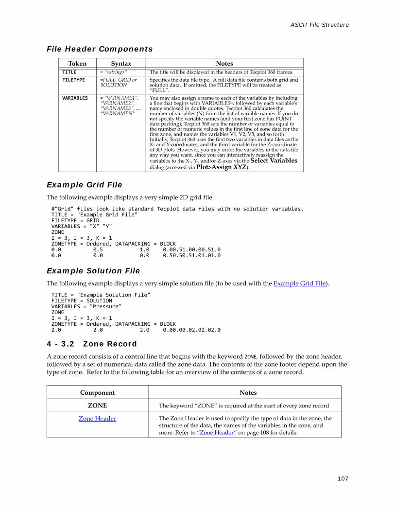
107
ASCII File Structure
File Header Components
Example Grid FileThe following example displays a very simple 2D grid file.
#"Grid" files look like standard Tecplot data files with no solution variables.TITLE = "Example Grid File"FILETYPE = GRIDVARIABLES = "X" "Y"ZONEI = 3, J = 3, K = 1ZONETYPE = Ordered, DATAPACKING = BLOCK0.0 0.5 1.0 0.00.51.00.00.51.00.0 0.0 0.0 0.50.50.51.01.01.0
Example Solution FileThe following example displays a very simple solution file (to be used with the Example Grid File).
TITLE = "Example Solution File"FILETYPE = SOLUTIONVARIABLES = "Pressure"ZONEI = 3, J = 3, K = 1ZONETYPE = Ordered, DATAPACKING = BLOCK2.0 2.0 2.0 0.00.00.02.02.02.0
4 - 3.2 Zone RecordA zone record consists of a control line that begins with the keyword ZONE, followed by the zone header, followed by a set of numerical data called the zone data. The contents of the zone footer depend upon the type of zone. Refer to the following table for an overview of the contents of a zone record.
Token Syntax NotesTITLE = “<string>” The title will be displayed in the headers of Tecplot 360 frames. FILETYPE =FULL, GRID or
SOLUTIONSpecifies the data file type. A full data file contains both grid and solution data. If omitted, the FILETYPE will be treated as “FULL”.
VARIABLES = “VARNAME1”, “VARNAME2”, “VARNAME3”, ..., “VARNAMEN”
You may also assign a name to each of the variables by including a line that begins with VARIABLES=, followed by each variable’s name enclosed in double quotes. Tecplot 360 calculates the number of variables (N) from the list of variable names. If you do not specify the variable names (and your first zone has POINT data packing), Tecplot 360 sets the number of variables equal to the number of numeric values in the first line of zone data for the first zone, and names the variables V1, V2, V3, and so forth. Initially, Tecplot 360 uses the first two variables in data files as the X- and Y-coordinates, and the third variable for the Z-coordinate of 3D plots. However, you may order the variables in the data file any way you want, since you can interactively reassign the variables to the X-, Y-, and/or Z-axes via the Select Variables dialog (accessed via Plot>Assign XYZ).
Component Notes
ZONE The keyword “ZONE” is required at the start of every zone record
Zone Header The Zone Header is used to specify the type of data in the zone, the structure of the data, the names of the variables in the zone, and more. Refer to “Zone Header” on page 108 for details.

108
Zone Header
Data The data section follows the zone header. The arrangement of the data is dependent upon the values of DATA PACKING and VAR LOCATION (specified in the Zone Header). Refer to “Data” on page 111 for details.
Zone Footer The contents required for the Zone Footer depend upon the ZONETYPE (specified in the Zone Header). For ordered zones, the Zone Footer contains the Face Neighbor Connections List information (if any).For cell-based finite element zones (FETRIANGLE, FEQUADILATERAL, FETETRAHEDRAL and FEBRICK), the Zone Footer contains Connectivity information, followed by Face Neighbor Connections List.For face-based finite element zones (FEPOLYHEDRAL, FEPOLYGON), the Zone Footer contains Facemap Data, followed by Boundary Map Data.Refer to “Zone Footer” on page 113 for additional information.
Keyword Syntax Required(Y/N)
Default Notes
ZONE Y Keyword required to start a zone recordT = <string> N Zone Title. This may be any text string up to 128
characters in length. If you supply a longer text string, it is automatically truncated to the first 128 characters. The titles of zones appear in the Zone Style and other dialogs, and, optionally, in the XY- plot legend.
ZONETYPE = <zonetype> N ORDERED
The zone data are of the type specified by the ZONETYPE parameter in the control line. There are two basic types of zones: ordered and finite element. ORDERED is presumed if the ZONETYPE parameter is omitted. See Section 4 - 4 “Ordered Data” for more information on ordered zones, and Section 4 - 5 “Finite Element Data” for details on finite element data.
When specifying your ZoneType, please note that some features in Tecplot 360are limited by zone type. For example, iso-surfaces and slices are available for 3D zones types only (FETETRAHEDRON, FEBRICK,FEPOLYHEDRON and ORDERED - with K greater than 1).
However, the plot type that you specify (in Tecplot 360 once you have loaded your data) is not limited by your zone type. You may have a 3D zone displayed in a 2D Cartesian plot (and visa versa).
I = <integer> Y Specify the maximum number of points in the I- J- or K-direction. Use only when ZONETYPE is ORDERED.J = <integer> Y
K = <integer> YNODES = <integer> Y Use for finite element zone types only (that is, not
ordered zones). Specify the total number of NODES and ELEMENTS in the data file. Refer to Section 4 - 5 “Finite Element Data” for additional information.
ELEMENTS = <integer> Y
FACES = <integer> Y (for face-based finite element zones)
Use for face-based finite element zones types (polygonal and polyhedral) only. Specify the number of FACES in the data file. See Section 4 - 5 “Finite Element Data” for more information.
TOTALNUMFACENODES
= <integer> Y (for polyhedral zones)
For face-based finite element zones only. Total number of nodes in the Facemap Data section for all faces. This is optional for polygons as TotalNumFaceNodes = 2*NumFaces.
NUMCONNECTEDBOUNDARYFACES
= <integer> Y For face-based finite element zones only. Total number of boundary faces listed in the Facemap Data section. Set to zero if boundary faces aren't used.

109
ASCII File Structure
TOTALNUMBOUNDARYCONNECTIONS
= <integer> Y For face-based finite element zones only. Total number of entries for boundary items listed in the Facemap Data section. Set to zero if boundary faces aren't used.
FACENEIGHBORMODE
= [LOCALONETOONE, LOCALONETOMANY, GLOBALONETOONE, GLOBALONETOMANY]
N LOCALONETOONE
For ordered or cell-based finite element zones only. Used to indicate whether the neighboring faces are within the current zone or in another zone (i.e. local or global), as well as whether the connections are one-to-one or one-to-many. When this token is used, both the FACENEIGHBORCONNECTIONS token and the FaceNeighbor Connections List are required. Refer to Section “Face Neighbor Connections List” on page 113 for details.
FACENEIGHBORCONNECTIONS
= <integer> Y, if FACENEIGHBORMODE,is in use.
For ordered or cell-based finite element zones only. Used to indicate the total number of connections for all elements in the zone. For example, if you have two cells with three connections each, the number of face neighbor connections is equal to six. When this token is used, both the FACENEIGHBORMODE token and the FaceNeighbor Connections List are required. Refer to Section “Face Neighbor Connections List” on page 113 for details.
DT = (<datatype> for var1, <datatype> for var2, ..., <datatype> for varn)
N SINGLE Each variable in each zone in the data file may have its own data type. The data type determines the amount of storage Tecplot 360 assigns to each variable. Therefore, the lowest level data type should be used whenever possible. For example, imaging data, which usually consists of numerical values ranging from zero to 255, should be given a data type of BYTE. By default, Tecplot 360 treats numeric data as data type SINGLE. If any variable in the zone uses the BIT data type, the DATA PACKING must be BLOCK. Refer to “Data” on page 111 for details.
DATAPACKING
= <datapacking> N BLOCK In POINT format, the values for all variables are given for the first point, then the second point, and so on. In BLOCK format, all of the values for the first variable are given in a block, then all of the values for the second variable, then all of the values for the third, and so forth. BLOCK format must be used for cell-centered data and polyhedral zones (FEPOLYGON/FEPOLYHEDRAL), as well as for all binary data.
VARLOCATION
=([set-of-vars]=<varlocation>,[set-of-vars]=<varlocation>, ...)
N NODAL Each variable in each zone in a data file may be located at the nodes or the cell-centers. Each variable is specified as NODAL or CELLCENTERED in the VARLOCATION parameter array. All cell-centered variables must list one value for each element. With nodal variables, one value must be listed for each node. Zones with cell-centered variables must be in BLOCK data packing format.
VARSHARELIST
=([set-of-vars]= <zone>, [set-of-vars]=<zone>)
N If zone number is omitted, the variables are shared from the previous zone.
Used for variables that are exactly the same for a set of zones. Specify the integer value of the source zone. Ordered zones may only share with ordered zones having the same dimensions. Finite element zones may share with any zone having the same number of nodes, for nodal variables, or the same number of cells, for cell-centered data.
NV = <integer> N Specifies the variable number of the variable representing the “Node” value in finite element data. The NV parameter is used infrequently. It is mostly used when the order in which nodes are listed in the data file does not match the node numbering desired in the plot. Refer to Section “Finite Element Zone Node Variable Parameters Example” on page 137 for an example using the NV parameter.
Keyword Syntax Required(Y/N)
Default Notes

110
CONNECTIVITYSHAREZONE
=<zone> N Specify the number of the zone from which the connectivity is shared. The connectivity list (cell-basedfinite element only) and face-neighbors may be shared between zones using the CONNECTIVITYSHAREZONE parameter in the control line of the current zone. Alternatively, the parameter may be used to share the Facemap Data for face-based finite element zones.To use connectivity sharing, the zone must have the same number of points and elements (and faces, if the zone is face-based), and be the same zone type.
STRANDID = <integer> N Each zone can optionally specify an integer value associating itself with a particular strand. More than one zone can associate itself with a particular strand and differentiate itself from other zones by assigning different SOLUTIONTIME values. StrandID's must be positive integer values greater than or equal to 1. By convention strandID's are successive integer values.
SOLUTIONTIME
= <double> N Specify a floating point time value representing the solution time. Zones can be organized together by associating themselves to the same STRANDID.
PARENTZONE = <zone> N Scalar integer value representing the relationship between this zone and its parent. A value of zero indicates that this zone is not associated with a parent zone. A value greater than zero is considered this zone's parent. A zone may not specify itself as its own parent. With a parent zone association, Tecplot 360 can generate a surface streamtrace on a no-slip boundary zone. Refer to Section 15 - 2 “Surface Streamtraces on No-slip Boundaries” in the User’s Manual for additional information.
PASSIVEVARLIST
= [set of vars] N All variables non-passive
Use this option to make variables passive. For example, to make variables 4, 5, and 20 passive, use this syntax: PASSIVEVARLIST=[4-5,20]See Section 1 - 3 “Best Practices”, Section 7. “Passive Variables” for information on passive variables.
AUXDATA NAME = <string> N Auxiliary data strings associated with the current zone are specified with the AUXDATA parameter in the control line. This auxiliary data may be used in dynamic text, equations, macros, or add-ons. There may be multiple AUXDATA parameters in the control line for a zone, but names must be unique. NOTE: The NAME portion of the string cannot contain spaces.Auxiliary data is provided as named strings: AUXDATA EXPERIMENTDATE ="October 13, 2007, 8 A.M."
Keyword Syntax Required(Y/N)
Default Notes

111
ASCII File Structure
DataTecplot 360 supports the following six data types:
• DOUBLE (eight-byte floating point values).• SINGLE (four-byte floating point values).• LONGINT (four-byte integer values).• SHORTINT (two-byte integer values).• BYTE (one-byte integer values, from zero to 255).• BIT
The arrangement of ASCII data depends upon the combination of datapacking (BLOCK or POINT), variable location (NODAL or CELL-CENTERED). The zone type also plays a role in that not all forms of datapacking and variable locations are supported by all zone types. In BLOCK data, the data is arranged by variable, while in POINT data the data is arranged by point (node or data point, depending upon the zone type). In NODAL data the variable values are defined at every node (FE data) or point (ORDERED data). In CELLCENTERED data, the variable values are defined at the center of every cell (ORDERED data) or element (FE data).
The available combinations of datapacking and variable location parameters are:
• Block - Nodal• Block - Cell-centered• Point - Nodal
The combination of POINT and CELLCENTERED is not available.
BLOCK - NODALIn block data with nodal values, the data is arranged by variable and each variable is defined at the nodes. The data arrangement is as follows:
A11 A12 ... A1PA21 A22 ... A2P...
AV1 AV2 ... AVP
where:
V = total number of nonpassive, nonshared variablesP = I * J * K (ordered zones) orNODES(FE zones)
BLOCK - CELLCENTEREDIn block data with cell-centered values, the data is arranged by variable and each variable is defined at the center of each cell (ORDERED data) or element (FE data). The data arrangement is as follows:
A11 A12 ... A1PA21 A22 ... A2P...AV1 AV2 ... AVP
where:
V = total number of nonpassive, nonshared variables

112
P = (I -1) * (J - 1) * (K -1) (ordered zones1) or
P = ELEMENTS (FE zones)
POINT - NODALIn point data, the values for all variables are given for the first point, then the second point and so on. The variable location is always NODAL.
A11 A12 ... A1VA21 A22 ... A2V...AP1 AP2 ... APV
where:
V = total number of nonpassive, nonshared variablesP = I * J * K (ordered zones)
orP = ELEMENTS (FE zones)
General Formatting RulesThe following formatting guidelines apply to all data arrangements:
• Numerical values in zone data must be separated by one or more spaces, commas, tabs, new lines, or carriage returns. The radix (decimal point) is ‘.‘ (period) even in locales that use another character, such as ‘,‘ (comma).
• Blank lines are ignored.• Integer (101325), floating point (101325.0), and exponential (1.01325E+05) numbers are accepted. • To repeat a particular number in the data, precede it with a repetition number as follows:
“Rep*Num,” where Rep is the repetition factor and Num is some numeric value to be repeated. For example, you may represent 37 values of 120.5 followed by 100 values of 0.0 as follows:
37*120.5, 100*0.0
Variable SharingFrequently, some variables are exactly the same for a set of zones. For example, a series of zones may contain measurement or simulation data at the same XYZ-locations, but different times. In this case, Tecplot 360’s memory usage may be dramatically reduced by sharing the coordinate variables between the zones. The zones that variables are shared from are specified in the VARSHARELIST in the control line of the current zone. The format is:
VARSHARELIST=([set-of-vars]=zzz, [set-of-vars]=zzz)
where set-of-vars is the set of variables that are shared and zzz is the zone they are shared from. If zzz is omitted, the variables are shared from the previous zone.
For example:
VARSHARELIST=([4-6,11]=3, [20-23]=1, [13,15])
specifies that variables four, five, six and 11 are shared from zone three, variables 20, 21, 22, and 23 are shared from zone one, and variables 13 and 15 are shared from the previous zone. For variable sharing, ordered zones may only share with ordered zones having the same dimensions. Finite element zones may
1. For all I, J and K greater than one. When I, J or K is equal to one, a value of one is used instead of subtract-ing one.

113
ASCII File Structure
share with any zone having the same number of nodes (for nodal variables) or the same number of cells (for cell-centered data).
Zone FooterThe contents required for the Zone Footer depend upon the ZONETYPE (specified in the Zone Header).
• Ordered zones - the Zone Footer contains the Face Neighbor Connections List (if any).• Cell-based finite element zones (FETRIANGLE, FEQUADILATERAL, FETETRAHEDRAL
and FEBRICK) - the Zone Footer contains Connectivity information, followed by Face Neighbor Connections List (if any).
• Face-based finite element zones (FEPOLYHEDRAL, FEPOLYGON) - the Zone Footer contains Facemap Data, followed by Boundary Map Data.
ConnectivityFor cell-based finite element zones (FETRIANGLE, FEQUADILATERAL, FETETRAHEDRAL, and FEBRICK), the nodal data is followed by the connectivity information. The connectivity list is not preceded by a token or keyword. It is simply a list of numbers.
The connectivity list details the node numbers of all of the nodes included in each element. When providing the connectivity list, please keep in mind the following guidelines:
• Each row in the connectivity list corresponds to an element, where the first row corresponds to the first element, and so forth.
• The node numbers must be provided in order, either clockwise or counter-clockwise.• You must provide the same number of nodes as are included in an element. For example, you
must provide eight numbers for BRICK elements and three numbers for TRIANGLE elements. If you are using repeated nodes, provide the node number of the repeated node multiple times.
See also: “Connectivity Sharing” on page 116.
The connectivity for face-based zones (FEPOLYGON and FEPOLYHEDRAL) is defined by the Facemap Data (refer to “Facemap Data” on page 115 for details).
Face Neighbor Connections ListFor ordered zones, the data section may be followed with face neighbor connections. For cell-based finite element zones, the data section and connectivity list may be followed by the face neighbor connection information.
Use face neighbors to specify connections between zones (global connections) or connections within zones (local connections). Face neighbor connections are used by Tecplot when deriving variables or drawing contour lines. Specifying face neighbors, typically leads to smoother connections. NOTE: face neighbors have expensive performance implications. Use face neighbors to manually specify connections that are not defined via the connectivity list.
Face neighbor connections are defined by the FACENEIGHBORMODE and FACENEIGHBORCONNECTIONS tokens along with the Face Neighbor Connections list. The FACENEIGHBORMODE token is used to specify the type of face neighbor connection used. The FACENEIGHBORCONNECTIONS token is used to define the total number of face neighbor connections included in the zone.
The nature of the data arranged in the Face Neighbor Connections list depends upon the FACENEIGHBORMODE, described in the table below. To connect the cells along one edge to cells on another edge of the same zone, use LOCAL. To connect cells of one zone to cells of another zone or zones, use GLOBAL. If the

114
points of the cells are exactly aligned with the neighboring cell points, use ONETOONE. If even one cell face is neighbor to two or more other cell faces, use ONETOMANY.
In this table,
• cz -the cell number in the current zone• fz - the number of the cell face in the current zone• nc -the cell number of the neighbor cell in the current zone• oz - face obscuration flag (zero for face partially obscured, one for face entirely obscured)• nz - the number of neighboring cells for the ONETOMANY options• ncn - the number of the nth local zone neighboring cell in the list• zr - the remote zone number• cr - the cell number of the neighboring cell in the remote zone• zrn - the zone number of the nth neighboring cell in the GLOBALONETOMANY list• crn - the cell number in the remote zone of the nth neighboring cell in the GLOBALONETOMANY list.
The cz, fz combinations must be unique; multiple entries are not allowed. The face numbers for cells in thevarious zone types are defined in Figure 4-1..
Figure 4-1. A: Example of node and face neighbors for an FE-brick cell or IJK-ordered cell. B: Example of node and face numbering for an IJ-ordered/ FE-quadrilateral cell. C: Example of tetrahedron face neighbors.
A connection must be specified for two matching cell faces to be effective. The nature of the Face Neighbor Connections list depends upon its FACENEIGHBORMODE.
For example, for data with a FACENEIGHBORMODE of GLOBALONETOONE, if cell six, face two in zone nine should be connected to cell one, face four in zone 10, the connections for zone nine must include the line:
6 2 10 1 (cell#, face#, connecting zone#, connecting cell#)
Mode Number of Values Order of Data in the Face Neighbor Connections List
LOCALONETOONE 3 cz, fz, nc
LOCALONETOMANY nz+4 cz, fz, oz, nz, nc1, nc2, ..., ncn
GLOBALONETOONE 4 cz, fz, zr, cr
GLOBALONETOMANY 2*nz+4 cz, fz, oz, nz, zrl, crl, zr2, cr2, ..., zrn, crn
A B C
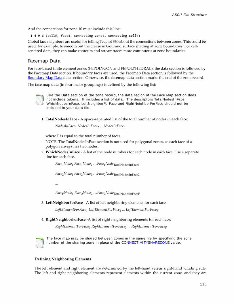
115
ASCII File Structure
And the connections for zone 10 must include this line:
1 4 9 6 (cell#, face#, connecting zone#, connecting cell#)
Global face neighbors are useful for telling Tecplot 360 about the connections between zones. This could be used, for example, to smooth out the crease in Gouraud surface shading at zone boundaries. For cell-centered data, they can make contours and streamtraces more continuous at zone boundaries.
Facemap DataFor face-based finite element zones (FEPOLYGON and FEPOLYHEDRAL), the data section is followed by the Facemap Data section. If boundary faces are used, the Facemap Data section is followed by the Boundary Map Data data section. Otherwise, the facemap data section marks the end of the zone record.
The face map data (in four major groupings) is defined by the following list:
1. TotalNodesInFace - A space-separated list of the total number of nodes in each face:
NodesInFace1 NodesInFace2 …NodesInFaceF
where F is equal to the total number of faces.NOTE: The TotalNodesInFace section is not used for polygonal zones, as each face of a polygon always has two nodes.
2. WhichNodesInFace - A list of the node numbers for each node in each face. Use a separate line for each face.
Face1Node1 Face1Node2 …Face1NodeTotalNodesInFace1
Face2Node1 Face2Node2 …Face2NodeTotalNodesInFace2
...
FaceFNode1 Face2Node2 …Face2NodeTotalNodesInFaceF
3. LeftNeighborForFace - A list of left neighboring elements for each face:
LeftElementForFace1 LeftElementForFace2 ... LeftElementForFaceF
4. RightNeighborForFace -A list of right neighboring elements for each face:
RightElementForFace1 RightElementForFace2 ... RightElementForFaceF
Defining Neighboring Elements
The left element and right element are determined by the left-hand versus right-hand winding rule.The left and right neighboring elements represent elements within the current zone, and they are
Like the Data section of the zone record, the data region of the Face Map section does not include tokens. It includes a list of data. The descriptors TotalNodesInFace, WhichNodesInFace, LeftNeighborForFace and RightNeighborForFace should not be included in your data file.
The face map may be shared between zones in the same file by specifying the zone number of the sharing zone in place of the CONNECTIVITYSHAREZONE value.
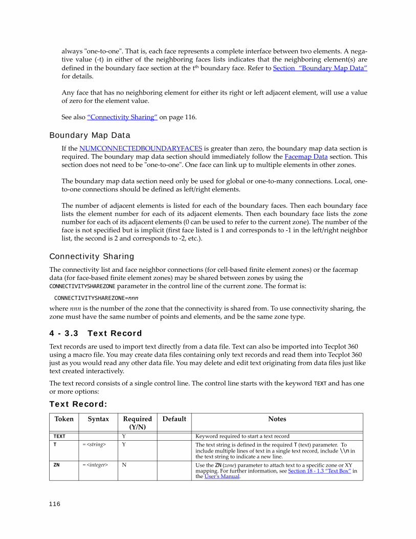
116
always "one-to-one". That is, each face represents a complete interface between two elements. A nega-tive value (-t) in either of the neighboring faces lists indicates that the neighboring element(s) aredefined in the boundary face section at the tth boundary face. Refer to Section “Boundary Map Data”for details.
Any face that has no neighboring element for either its right or left adjacent element, will use a valueof zero for the element value.
See also “Connectivity Sharing” on page 116.
Boundary Map DataIf the NUMCONNECTEDBOUNDARYFACES is greater than zero, the boundary map data section isrequired. The boundary map data section should immediately follow the Facemap Data section. Thissection does not need to be "one-to-one". One face can link up to multiple elements in other zones.
The boundary map data section need only be used for global or one-to-many connections. Local, one-to-one connections should be defined as left/right elements.
The number of adjacent elements is listed for each of the boundary faces. Then each boundary facelists the element number for each of its adjacent elements. Then each boundary face lists the zonenumber for each of its adjacent elements (0 can be used to refer to the current zone). The number of theface is not specified but is implicit (first face listed is 1 and corresponds to -1 in the left/right neighborlist, the second is 2 and corresponds to -2, etc.).
Connectivity SharingThe connectivity list and face neighbor connections (for cell-based finite element zones) or the facemap data (for face-based finite element zones) may be shared between zones by using the CONNECTIVITYSHAREZONE parameter in the control line of the current zone. The format is:
CONNECTIVITYSHAREZONE=nnn
where nnn is the number of the zone that the connectivity is shared from. To use connectivity sharing, the zone must have the same number of points and elements, and be the same zone type.
4 - 3.3 Text RecordText records are used to import text directly from a data file. Text can also be imported into Tecplot 360 using a macro file. You may create data files containing only text records and read them into Tecplot 360 just as you would read any other data file. You may delete and edit text originating from data files just like text created interactively.
The text record consists of a single control line. The control line starts with the keyword TEXT and has one or more options:
Text Record:
Token Syntax Required (Y/N)
Default Notes
TEXT Y Keyword required to start a text recordT = <string> Y The text string is defined in the required T (text) parameter. To
include multiple lines of text in a single text record, include \\n in the text string to indicate a new line.
ZN = <integer> N Use the ZN (zone) parameter to attach text to a specific zone or XY mapping. For further information, see Section 18 - 1.3 “Text Box” in the User’s Manual.
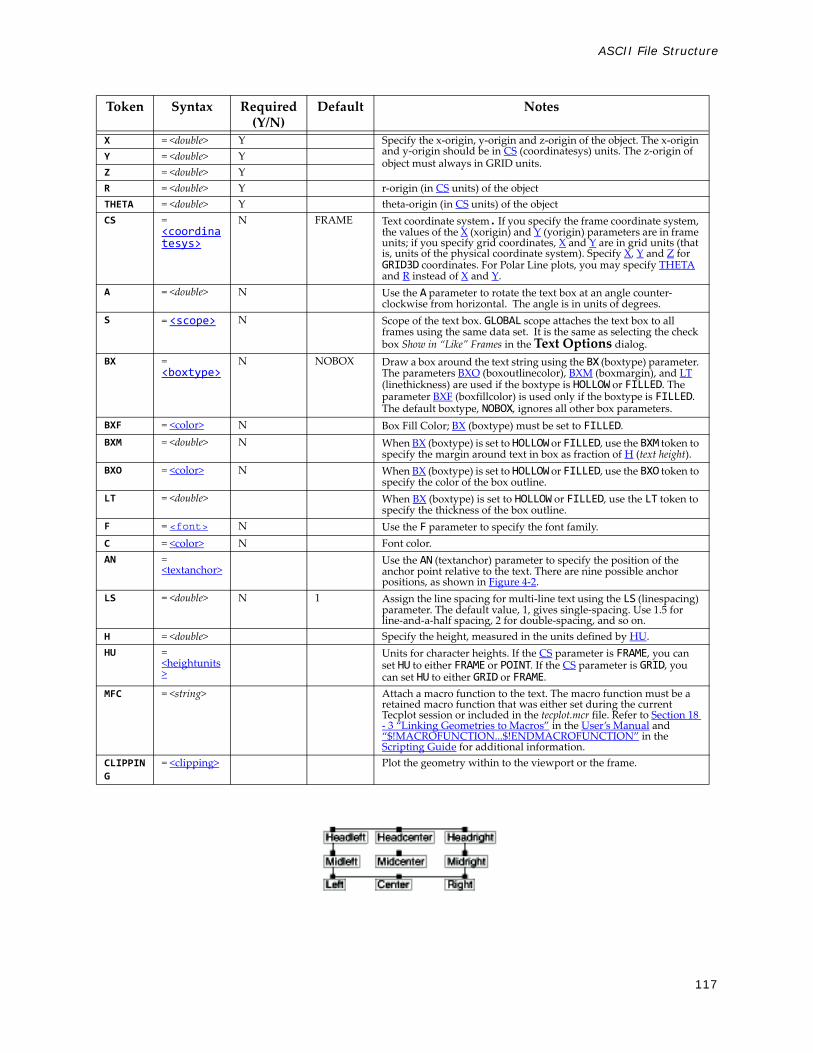
117
ASCII File Structure
X = <double> Y Specify the x-origin, y-origin and z-origin of the object. The x-origin and y-origin should be in CS (coordinatesys) units. The z-origin of object must always in GRID units. Y = <double> Y
Z = <double> YR = <double> Y r-origin (in CS units) of the object THETA = <double> Y theta-origin (in CS units) of the object CS =
<coordinatesys>
N FRAME Text coordinate system. If you specify the frame coordinate system, the values of the X (xorigin) and Y (yorigin) parameters are in frame units; if you specify grid coordinates, X and Y are in grid units (that is, units of the physical coordinate system). Specify X, Y and Z for GRID3D coordinates. For Polar Line plots, you may specify THETA and R instead of X and Y.
A = <double> N Use the A parameter to rotate the text box at an angle counter-clockwise from horizontal. The angle is in units of degrees.
S = <scope> N Scope of the text box. GLOBAL scope attaches the text box to all frames using the same data set. It is the same as selecting the check box Show in “Like” Frames in the Text Options dialog.
BX = <boxtype>
N NOBOX Draw a box around the text string using the BX (boxtype) parameter. The parameters BXO (boxoutlinecolor), BXM (boxmargin), and LT (linethickness) are used if the boxtype is HOLLOW or FILLED. The parameter BXF (boxfillcolor) is used only if the boxtype is FILLED. The default boxtype, NOBOX, ignores all other box parameters.
BXF = <color> N Box Fill Color; BX (boxtype) must be set to FILLED.BXM = <double> N When BX (boxtype) is set to HOLLOW or FILLED, use the BXM token to
specify the margin around text in box as fraction of H (text height).BXO = <color> N When BX (boxtype) is set to HOLLOW or FILLED, use the BXO token to
specify the color of the box outline. LT = <double> When BX (boxtype) is set to HOLLOW or FILLED, use the LT token to
specify the thickness of the box outline.F = <font> N Use the F parameter to specify the font family. C = <color> N Font color. AN =
<textanchor>Use the AN (textanchor) parameter to specify the position of the anchor point relative to the text. There are nine possible anchor positions, as shown in Figure 4-2.
LS = <double> N 1 Assign the line spacing for multi-line text using the LS (linespacing) parameter. The default value, 1, gives single-spacing. Use 1.5 for line-and-a-half spacing, 2 for double-spacing, and so on.
H = <double> Specify the height, measured in the units defined by HU.HU =
<heightunits>
Units for character heights. If the CS parameter is FRAME, you can set HU to either FRAME or POINT. If the CS parameter is GRID, you can set HU to either GRID or FRAME.
MFC = <string> Attach a macro function to the text. The macro function must be a retained macro function that was either set during the current Tecplot session or included in the tecplot.mcr file. Refer to Section 18 - 3 “Linking Geometries to Macros” in the User’s Manual and “$!MACROFUNCTION...$!ENDMACROFUNCTION” in the Scripting Guide for additional information.
CLIPPING
= <clipping> Plot the geometry within to the viewport or the frame.
Token Syntax Required (Y/N)
Default Notes

118
Figure 4-2. Text anchor positions—values for the AN parameter.

119
ASCII File Structure
Text Record ExamplesSome simple examples of text records are shown below. The first text record specifies only the origin and the text. The next text record specifies the origin, color, font, and the text. The third text record specifies the origin, height, box attributes, and text. Note that the control line for the text can span multiple file lines if necessary (as in the third text record below). The last text record is an example of using 3D text in Tecplot 360.
TEXT X=50, Y=50, T="Example Text"TEXT X=10, Y=10, F=TIMES-BOLD, C=BLUE, T="Blue Text"TEXT X=25, Y=90, CS=FRAME, HU=POINT, H=14,BX=FILLED, BXF=YELLOW, BXO=BLACK, LS=1.5,T="Box Text \\n Multi-lined text"TEXT CS=GRID3D, X=0.23,Y=0.23,Z=0.5, T="Well 1"
4 - 3.4 Geometry RecordGeometry records are used to import geometries from a data file. Geometries are line drawings that may be boundaries, arrows, or even representations of physical structures. You may create data files containing only geometry and text records and read them into Tecplot 360. You may delete and edit geometries originating from data files just like the geometries that you create interactively.
The geometry record control line begins with the keyword GEOMETRY.

120
Geometry Record Contents
Data for Geometry RecordThe control line of the geometry is followed by geometry data. For SQUARE, the geometry data consists of just one number: the side length of the square.
For RECTANGLE, the geometry data consists of two numbers: the first is the width (horizontal axis dimension), and the second is the height (vertical axis dimension).
For CIRCLE, the geometry data is one number: the radius. For ELLIPSE, the geometry data consists of two numbers: the first is the horizontal axis length and the second is the vertical axis length. For both circles and ellipses, you can use the EP (numellipsepts) parameter to specify the number of points used to draw circles and ellipses. All computer-generated curves are simply collections of very short line segments; the EP parameter allows you to control how many line segments Tecplot 360 uses to approximate circles and ellipses. The default is 72.
Token Available Values NotesGEOMETRY Keyword required to start a geometry recordT = <geomtype> Geometry typeF = <datapacking> Geometry data formatDT = <datatype> Data typeZN = <integer> Attach text to a specific zone or XY mapping. For further information, see Section 18 - 1.3
“Text Box” in the User’s Manual.X = <double> Specify the x-origin, y-origin and z-origin of the object. The x-origin and y-origin should
be in CS (coordinatesys) units. The z-origin of object is for LINE3D geometries only and must always in GRID units. Refer to “Origin positions” for additional information regarding the origin location for each type of geometry.
Y = <double>Z = <double>
R = <double> Specify the r-origin and theta-origin of the object. The origins should be in CS units. Refer to Section “Origin positions” on page 121 for additional information.THETA = <double>
CS = <coordinatesys> Geometry coordinate system. If you specify the frame coordinate system, the values of the X (xorigin) and Y (yorigin) parameters are in frame units; if you specify grid coordinates, X and Y are in grid units (that is, units of the physical coordinate system). Specify X, Y and Z for GRID3D coordinates. For Polar Line plots, you may specify THETA and R instead of X and Y.
DRAWORDER = <draworder> Draw order.S = <scope> The S (scope) parameter specifies the text scope. GLOBAL scope attaches the text box to all
frames using the same data set. It is the same as selecting the check box Show in “Like” Frames in the Geometry Options dialog.
C = <color> Geometry outline color.L = <linetype> Line typePL = <double> Pattern length (in frame units).LT = <double> Line thickness (in frame units)EP = <integer> Number of points used to approximate circles or ellipsesFC = <color> Fill Color. Any geometry type except LINE3D may be filled with a color by using the FC
(fillcolor) parameter. Each polyline of a LINE geometry is filled individually (by connecting the last point of the polyline with the first). Not specifying the FC (fillcolor) parameter results in a hollow, or outlined, geometry drawn in the color of the C (color) parameter.
AST = <arrowheadstyle> Arrowhead styleAAT = N<arrowheadattach> Arrowhead attachment along the line geometryASZ = <double> Size of arrowhead in frame unitsAAN = <double> Angle of arrowhead in degreesMFC = <string> You may attach a macro function to the text with the MFC parameter. The macro function
must be a retained macro function that was either set during the current Tecplot session or included in the tecplot.mcr file. Refer to Section 18 - 3 “Linking Geometries to Macros” in the User’s Manual and “$!MACROFUNCTION...$!ENDMACROFUNCTION” on page 152 in the Scripting Guide for additional information.
CLIPPING = <clipping> plot the geometry within the viewport or the frame.

121
ASCII File Structure
For LINE and LINE3D geometries, the geometry data is controlled by the F (format) parameter. These geometries may be specified in either POINT or BLOCK format. By default, POINT format is assumed. Each geometry is specified by the total number of polylines, up to a maximum of 50 polylines, where each polyline can have up to 32,000 points. Each polyline is defined by a number of points and a series of XY- or XYZ- coordinate points between which the line segments are drawn. In POINT format, the XY- or XYZ-coordinates are given together for each point. In BLOCK format, all the X-values are listed, then all the Y-values, and (for LINE3D geometries) all the Z-values. All coordinates are relative to the X, Y, and Z specified on the control line. You can specify points in either single or double precision by setting the DT (datatype) parameter to either SINGLE or DOUBLE.
Origin positionsGeometry types are selected with the T (geomtype) parameter. The available geometry types are listed below:
• SQUARE - A square with lower left corner at X, Y.• RECTANGLE - A rectangle with lower left corner at X, Y.• CIRCLE - A circle centered at X, Y.• ELLIPSE - An ellipse centered at X, Y.• LINE - A set of 2D polylines (referred to as multi-polylines) anchored at X, Y.• LINE3D - A set of 3D polylines (referred to as multi-polylines) anchored at X, Y, Z.
Geometry Record Examples• Rectangle - The following geometry record defines a rectangle of 40 width and 30 height:
GEOMETRY T=RECTANGLE40 30 #WIDTH HEIGHT
• Circle - The following geometry record defines an origin and a red circle of 20 radius, with an origin of (75, 75) that is filled with blue:
GEOMETRY X=75, Y=75, T=CIRCLE, C=RED, FC=BLUE,CS=FRAME20 #RADIUS
• Polyline - The following geometry record defines an origin and two polylines, drawn using the Custom 3 color. The first polyline is composed of three points, the second of two points.
GEOMETRY X=50, Y=50, T=LINE, C=CUST32 #Number of polylines3 #Number of points in polyline 10 1 #X, Y coordinates of the point 1 in polyline 1 0 0 #X, Y coordinates of the point 2 in polyline 1 2 0 #X, Y coordinates of the point 3 in polyline 1 2 #Number of points in polyline 20 0 #X, Y coordinates of the point 1 in polyline 2 1 2 #X, Y coordinates of the point 2 in polyline 2
In BLOCK format, the same geometry appears as:GEOMETRY X=50, Y=50, T=LINE, C=CUST3, F=BLOCK, CS=FRAME2 #Number of polylines3 #Number of points in polyline 10 0 2 #X position of each point in polyline 11 0 0 #Y position of each point in polyline 12 #Number of points in polyline 20 1 #X position of each point in polyline 20 2 #y position of each point in polyline 2
• Ellipse - The next geometry record defines a purple ellipse with a horizontal axis length of 20 and a vertical axis length of 10, with an origin of (10, 70), that is filled with yellow.
GEOMETRY X=10, Y=70, T=ELLIPSE, C=PURPLE, FC=YELLOW20 10 #Horizontal Axis, Vertical Axis
• 3D polyline - The final geometry record is a 3D polyline with four points that is composed of one polyline using the default origin of (0, 0, 0):

122
GEOMETRY T=LINE3D1 #Number of polylines4 #Number of points in polyline 10 0 0 #X, Y, Z coordinates of point 11 2 2 .3 2 3 .4 1 2 #X, Y, Z coordinates of point 4
In BLOCK format, this geometry record can be written as follows:GEOMETRY T=LINE3D, F=BLOCK1 #Number of polylines4 #Number of points in polyline 10 1 3 4 #X position for each point in the polyline0 2 2 1 #Y position for each point in the polyline0 2 3 2 #Z position for each point in the polyline
4 - 3.5 Custom Labels RecordThe custom label record is an optional record used to provide custom labels for axes, the contour legend or value labels. A single custom label record begins with the keyword CUSTOMLABELS, followed by a series of text strings. The first custom label string corresponds to a value of one on the axis, the next to a value of two, and so forth.
You may have up to ten custom label records in a data file. The custom label set to use is specified via the Tecplot interface. Refer to Section 17 - 8 “Axis Title Options” in the User’s Manual for details.
A simple example of a custom-label record is shown below. MON corresponds to a value of 1, TUE corresponds to 2, WED to 3, THU to 4, and FRI to 5. Since custom labels have a wrap-around effect, MON also corresponds to the values 6, 11, and so forth.
CUSTOMLABELS "MON", "TUE", "WED", "THU", "FRI"
You may include \n in a custom label to indicate that the following text should start a new line. For example,"Jan\n2012" appears in Tecplot 360 as:
Jan2012
4 - 3.6 Data Set Auxiliary Data RecordThere is frequently auxiliary data (or Metadata) that helps describe the data set. For example, experimental data may have information about the facility and time at which the data was taken, and other parameters that describe the experiment. Likewise, simulation results have auxiliary data (such as reference quantities for non-dimensional data) needed to fully analyze and present the results.
Auxiliary data are name/value pairs that a user can specify and then use in Tecplot 360 with dynamic text, equations, macros, or add-ons. This data may be with respect to the data set as a whole or it can vary from zone to zone. The ASCII file format token for specifying auxiliary data associated with the entire data set is DATASETAUXDATA, described here. Auxiliary data for a given variable is defined by VARAUXDATA, described in Section 4 - 3.7 “Variable Auxiliary Data Record”. Auxiliary data for a given zone is defined by the AUXDATA token within the zone record (refer to “Zone Header” on page 108 for details).
The data set auxiliary data control line is as follows:
DATASETAUXDATA name = “value”
where name is a unique character string with no spaces. You may have multiple DATASETAUXDATA records. However, the value of name must be unique for each record.
You must include a data set in order to use custom labels. You cannot use custom labels in files that contain only text and/or geometries.

123
ASCII File Structure
Auxiliary data may be used in text, macros, equations (if it is numeric), and accessed from add-ons. It may also be viewed directly in the AuxData page of the Data Set Information dialog.
Data Set Auxiliary Data ExamplesThe following auxiliary data contain flow field information that might be found in output from a computational fluid-dynamics simulation.
DATASETAUXDATA MachNo = "1.2"DATASETAUXDATA Alpha = "5"DATASETAUXDATA RefTemperature = "250"DATASETAUXDATA RefPressure = "101325"DATASETAUXDATA Configuration = "A2 No. 3"DATASETAUXDATA Date = "August 5, 2003"DATASETAUXDATA Region = "NE Quadrant of Sector 47"
You may then use the numerical values in equations to modify the variables as follows:
{P} = {P_non_dim} * AuxDataSet:RefPressure
Similar principles apply when using auxiliary data in text boxes or labels.
4 - 3.7 Variable Auxiliary Data RecordVariable auxiliary data is added to Tecplot 360 on a per variable basis. Like data set auxiliary data, multiple items can be added for each variable:
VARAUXDATA 1 MyData=”Hello”VARAUXDATA 1 MoreData=”World”VARAUXDATA 2 MyData=”More information”VARAUXDATA 2 MoreData=”hi mom”VARAUXDATA 2 MyExtraData=”Some extra data”
The variable number with which the auxiliary data is associated immediately follows the VARAUXDATA record. Also note that the data associated with a particular auxiliary data name are unique for each variable. Therefore the same named item can be added to each variable if desired. Conversely a particular auxiliary data item can be added to only one variable. NOTE: The name of an auxiliary data record cannot contain spaces.
4 - 3.8 ASCII Data File Parameter Assignment ValuesThe following parameters assignment values are shared among the following types of ASCII file records: Zone Record, Text Record, and/or Geometry Record. Refer to those sections for details.
Table 4:
<arrowheadstyle> PLAIN, HOLLOW, FILLED
<arrowheadattach> NONE, BEGINNING, END, BOTH
<boxtype> NOBOX, HOLLOW ,FILLED
<clipping> CLIPTOVIEWPORT, CLIPTOFRAME
<color> BLACK, RED, GREEN, BLUE, CYAN, YELLOW, PURPLE, WHITE, CUST1, ..., CUST8
<coordinatesys> FRAME, GRID, GRID3D
<datapacking> BLOCK, POINT
<datatype> SINGLE, DOUBLE

124
4 - 4 Ordered DataFor ordered data, the numerical values in the zone data must be in either POINT or BLOCK format, specified by the DATAPACKING parameter.
4 - 4.1 I-Ordered DataI-ordered data has only one index, the I-index. This type of data is typically used for XY-plots, scatter plots, and irregular (random) data for triangulation or for interpolation into an IJ-or IJK-ordered zone within Tecplot 360.
In I-ordered data, the I-index varies from one to IMax. The total number of data points is IMax. For zones with only nodal variables, the total number of values in the zone data is IMax*N (where N is the number of variables). For a mixture of nodal and cell-centered variables, the number of values in the zone data is IMax*Nn+(IMax-1)*Nc, where Nn is the number of nodal variables and Nc is the number of cell-centered variables. For data in POINT format, IMax is calculated by Tecplot 360 from the zone data if it is not explicitly set by the zone control line (using the I-parameter).
4 - 4.2 IJ-Ordered DataIJ-ordered data has two indices: I and J. IJ-ordered data is typically used for 2D and 3D surface mesh, contour, vector, and shade plots, but it can also be used to plot families of lines in XY-plots. Refer to Chapter 3: “Data Structure” in the User’s Manual for more information on data structure. In IJ-ordered data, the I-index varies from one to IMax, and the J-index varies from one to JMax. The total number of data points (nodes) is IMax*JMax. For zones with only nodal variables, the total number of numerical values in the zone data is IMax*JMax*N (where N is the number of variables). For a mixture of nodal and cell-centered variables, the number of values in the zone data is IMax*JMax*Nn+(IMax-1)*(JMax-1)*Nc, where Nn is the number of nodal variables and Nc is the number of cell-centered variables. Both IMax and JMax must be specified in the zone control line (with the I and J parameters). The I- and J-indices should not be confused with the X- and Y-coordinates—on occasions the two may coincide, but this is not the typical case.
<draworder> AFTERDATA,BEFOREDATA
<font> HELV, HELV-BOLD, TIMES, TIMES-ITALIC, TIMES-BOLD, TIMES-ITALIC-BOLD, COURIER, COURIER-BOLD, GREEK, MATH, USER-DEF
<geomtype> LINE, SQUARE, RECTANGLE, CIRCLE, ELLIPSE
<heightunits> In FRAME coordinatesys either FRAME or POINT; in GRID coordinatesys either GRID or FRAME.
<linetype> SOLID, DASHED, DASHDOT, DOTTED, LONGDASH, DASHDOTDOT
<scope> GLOBAL, LOCAL
<textanchor> LEFT, CENTER, RIGHT, MIDLEFT, MIDCENTER, MIDRIGHT, HEADLEFT, HEADCENTER, HEADRIGHT
<varlocation> NODAL, CELLCENTERED
<zone> zone number to which this item is assigned (0=all)
<zonetype> ORDERED, FELINESEG, FETRIANGLE, FEQUADRILATERAL, FETETRAHEDRON, FEBRICK, FEPOLYGON or FEPOLYHEDRAL
Table 4:

125
Ordered Data
The I-index varies the fastest. That is, when you write programs to print IJ-ordered data, the I-index is the inner loop and the J-index is the outer loop. Note the similarity between I-ordered data and IJ-ordered data with JMax=1.
4 - 4.3 IJK-Ordered DataIJK-ordered data has three indices: I, J, and K. This type of data is typically used for 3D volume plots, although planes of the data can be used for 2D and 3D surface plots. See Section “Ordered Data” in the User’s Manual for more information.
In IJK-ordered data, the I-index varies from one to IMax, the J-index varies from one to JMax, and the K-index varies from one to KMax. The total number of data points (nodes) is IMax*JMax*KMax. For zones with only nodal variables, the total number of values in the zone data is IMax*JMax*KMax*N, where N is the number of variables. For a mixture of nodal and cell-centered variables, the number of values in the zone data is IMax*JMax*KMax*Nn+(IMax-1)*(JMax-1)*(KMax-1)*Nc, where Nn is the number of nodal variables and Nc is the number of cell-centered variables. The three indices, IMax, JMax, and KMax, must be specified in the zone control line using the I, J, and K-parameters.
The I-index varies the fastest; the J-index the next fastest; the K-index the slowest. If you write a program to print IJK-ordered data, the I-index is the inner loop, the K-index is the outer loop, and the J-index is the loop in between. Note the similarity between IJ-ordered data and IJK-ordered data with KMax=1.
4 - 4.4 Ordered Data ExamplesThe following examples are provided for your reference:
• I-Ordered Data - Simple example• IJ-Ordered Data - Simple Example• IJK-Ordered Data - Simple Example• Multi-Zone XY Line Plot• Multi-Zone XY Line Plot with Variable Sharing Example• Cell-Centered Data• Two-Dimensional Field Plots• Three-Dimensional Field Plots• Polygonal - simple example• Polyhedral - complex example
I-Ordered Data - Simple exampleThis data set is plotted in Figure 4-3; each data point is labeled with its I-index.

126
Figure 4-3. An I-ordered data set.
In this example, each column of zone data corresponds to a data point; each row to a variable.
VARIABLES = "X", "Y"ZONE I=5, DATAPACKING=BLOCK2 3 5 6 74 9 25 36 49
In BLOCK format all values of each variable are listed, one variable at a time.
FORTRAN CodeThe following sample FORTRAN code shows how to create I-ordered data in BLOCK format:
INTEGER VAR...WRITE (*,*) ´ZONE DATAPACKING=BLOCK, I=´, IMAXDO 1 VAR=1,NUMVARDO 1 I=1,IMAX WRITE (*,*) ARRAY(VAR,I)
1 CONTINUE
IJ-Ordered Data - Simple ExampleThere are four variables (X, Y, Temperature, Pressure) and six data points.
Figure 4-4. An IJ-ordered data set.
In this example, each column of data corresponds to a data point; each row to a variable.
VARIABLES = "X", "Y", "Temperature", "Pressure"ZONE I=2, J=3, DATAPACKING=BLOCK3 7 2 6 1 50 2 4 6 8 90 0 1 0 1 150 43 42 37 30 21
In BLOCK format, all IMax*JMax values of each variable are listed, one variable at a time. Within each variable block, all the values of a variable at each data point are listed.
FORTRAN CodeThe following sample FORTRAN code shows how to create IJ-ordered data in BLOCK format:

127
Ordered Data
INTEGER VAR...WRITE (*,*) ´ZONE DATAPACKING=BLOCK, I=´, IMAX, ´, J=´, JMAXDO 1 VAR=1,NUMVAR
DO 1 J=1,JMAX DO 1 I=1,IMAX WRITE (*,*) ARRAY(VAR,I,J)1 CONTINUE
IJK-Ordered Data - Simple ExampleAn example of IJK-ordered data in BLOCK format is listed below. There are four variables (X, Y, Z, Temperature) and twelve data points.This data is plotted in Figure 4-5; each data point is labeled with its IJK-index.
Figure 4-5. An IJK-ordered data set.
For this example, each column of data corresponds to a data point; each row to a variable.
VARIABLES = "X" "Y" "Z" "Temp"ZONE I=3, J=2, K=2, DATAPACKING=BLOCK 0 3 6 0 3 6 0 3 6 0 3 6 0 0 0 6 6 6 0 0 0 6 6 6 0 1 3 3 4 6 8 9 11 11 12 14 0 5 10 10 41 72 0 29 66 66 130 169
FORTRAN CodeThe following sample FORTRAN code shows how to create an IJK-ordered zone in BLOCK format:
INTEGER VAR . . . . WRITE (*,*) ´ZONE DATAPACKING=BLOCK, I=´, IMAX, ´, J=´, JMAX, ´, K=´, KMAX DO 1 VAR=1,NUMVAR DO 1 K=1,KMAX
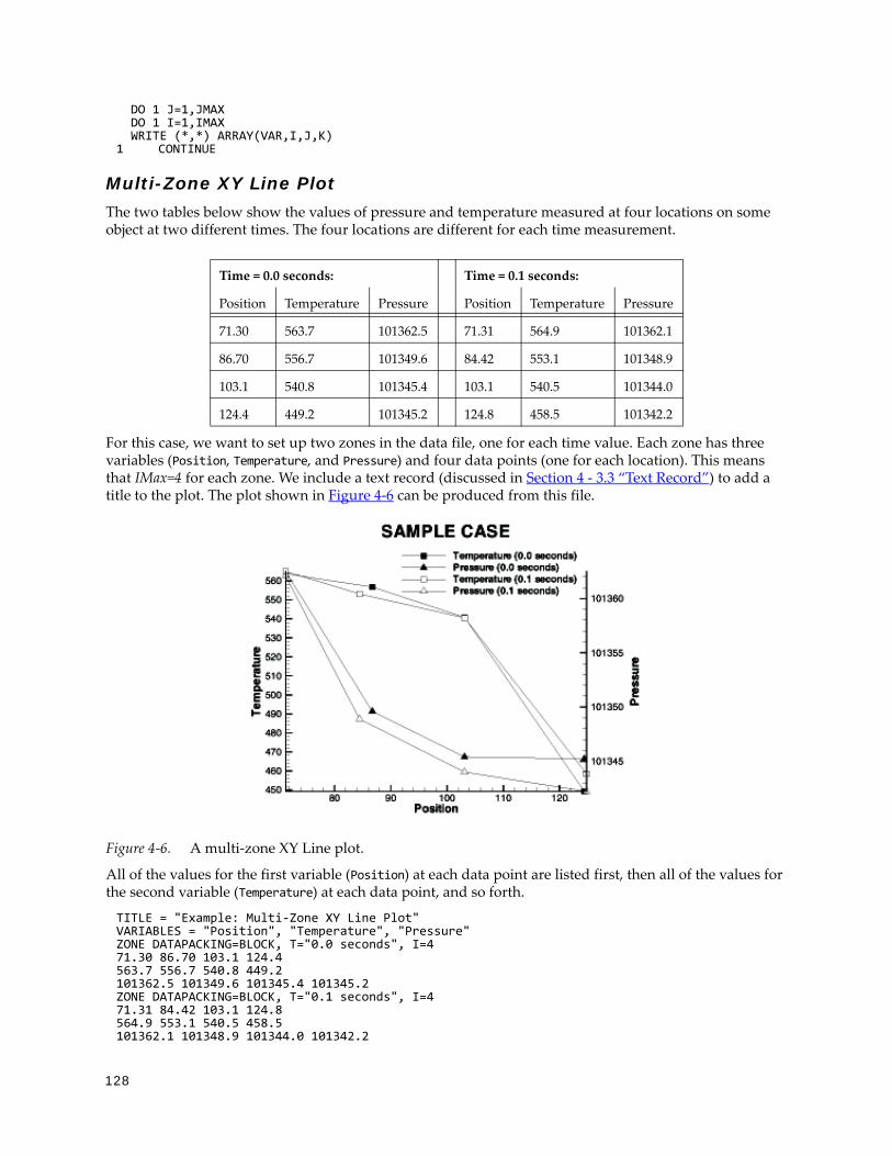
128
DO 1 J=1,JMAX DO 1 I=1,IMAX WRITE (*,*) ARRAY(VAR,I,J,K)1 CONTINUE
Multi-Zone XY Line PlotThe two tables below show the values of pressure and temperature measured at four locations on some object at two different times. The four locations are different for each time measurement.
For this case, we want to set up two zones in the data file, one for each time value. Each zone has three variables (Position, Temperature, and Pressure) and four data points (one for each location). This means that IMax=4 for each zone. We include a text record (discussed in Section 4 - 3.3 “Text Record”) to add a title to the plot. The plot shown in Figure 4-6 can be produced from this file.
Figure 4-6. A multi-zone XY Line plot.
All of the values for the first variable (Position) at each data point are listed first, then all of the values for the second variable (Temperature) at each data point, and so forth.
TITLE = "Example: Multi-Zone XY Line Plot"VARIABLES = "Position", "Temperature", "Pressure"ZONE DATAPACKING=BLOCK, T="0.0 seconds", I=471.30 86.70 103.1 124.4563.7 556.7 540.8 449.2101362.5 101349.6 101345.4 101345.2ZONE DATAPACKING=BLOCK, T="0.1 seconds", I=471.31 84.42 103.1 124.8564.9 553.1 540.5 458.5101362.1 101348.9 101344.0 101342.2
Time = 0.0 seconds: Time = 0.1 seconds:
Position Temperature Pressure Position Temperature Pressure
71.30 563.7 101362.5 71.31 564.9 101362.1
86.70 556.7 101349.6 84.42 553.1 101348.9
103.1 540.8 101345.4 103.1 540.5 101344.0
124.4 449.2 101345.2 124.8 458.5 101342.2

129
Ordered Data
TEXT CS=FRAME, HU=POINT, X=16, Y=90, H=28, T="SAMPLE CASE"
Multi-Zone XY Line Plot with Variable Sharing ExampleIf the data from the section above was taken at the same position for both times, variable sharing could reduce memory usage and file size. That file appears as:
TITLE = "Example: Multi-Zone XY Line Plot with Variable Sharing"VARIABLES = "Position", "Temperature", "Pressure"ZONE T="0.0 seconds", I=471.30 563.7 101362.586.70 556.7 101349.6103.1 540.8 101345.4124.4 449.2 101345.2ZONE T="0.1 seconds", I=4VARSHARELIST=([1]=1) #share variable 1 from zone 1564.9 101362.1553.1 101348.9540.5 101344.0458.5 101342.2TEXT CS=FRAME, HU=POINT, X=16, Y=90, H=28, T="SAMPLE VARIABLE SHARING CASE"
Cell-Centered DataAn example of IJ-ordered data with cell-centered variables might include four variables (X, Y, Temperature, Pressure), nine data points, and four cells where Temperature and Pressure are cell-ce
ntered.
Figure 4-7. An IJ-ordered data set with cell-centered data.
VARIABLES = "X", "Y", "Temperature", "Pressure"ZONE I=3, J=3, DATAPACKING=BLOCK, VARLOCATION=([3,4]=CELLCENTERED)3 7 11 2 6 10 1 5 90 2 3 4 6 8 8 9 100 2 1 345 60 35 70

130
The nodal variables of X and Y are specified at all nine nodes, and the values of cell-centered variables are specified at the four cells [(IMax-1)*(JMax-1)]. Zones with cell-centered data must have DATAPACKING=BLOCK.
Two-Dimensional Field PlotsA 2D field plot typically uses an IJ-ordered or finite element surface data set. However, any data structure can be viewed as a 2D field plot, by simply selecting “2D Cartesian” from the plot-type menu in the Plot sidebar.
An IJ-ordered data file has the basic structure shown below:
TITLE = "Example: Multi-Zone 2D Plot"VARIABLES = "X", "Y", "Press", "Temp", "Vel"ZONE T="BIG ZONE", I=3, J=3, DATAPACKING=POINT1.0 2.0 100.0 50.0 1.01.0 3.0 95.0 50.0 1.001.0 4.0 90.0 50.0 0.902.0 2.0 91.0 40.0 0.902.0 3.0 85.0 40.0 0.902.0 4.0 80.0 40.0 0.803.0 2.0 89.0 35.0 0.853.0 3.0 83.0 35.0 0.803.0 4.0 79.0 35.0 0.80ZONE T="SMALL ZONE", I=3, J=2, DATAPACKING=POINT3.0 2.0 89.0 35.0 0.853.5 2.0 80.0 35.0 0.854.0 2.0 78.0 35.0 0.803.0 3.0 83.0 35.0 0.803.5 3.0 80.0 35.0 0.854.0 3.0 77.0 33.0 0.78
This data file has two zones and five variables. The first zone has nine data points arranged in a three-by-three grid (I=3, J=3). Each row of each zone represents one data point, where each column corresponds to the value of each variable for a given data point, i.e. X = 1.0, Y = 2.0, Press = 100.0, Temp = 50.0, and Vel=- 1.0 for data point one in zone one (Big Zone).
Similarly, the second zone (Small Zone) has six data points in a three-by-two mesh (I=3, J=2). Reading this data file yields the mesh plot shown in Figure 4-12.
Refer to Section “Two-Dimensional Field Plots” on page 136 for an presentation of the same data in finite element format.
Three-Dimensional Field PlotsIJK-ordered data sets have the general form shown below:
TITLE = "Example: Simple 3D Volume Data"VARIABLES = "X", "Y", "Z", "Density"ZONE I=3, J=4, K=3, DATAPACKING=POINT1.0 2.0 1.1 2.212.0 2.1 1.2 5.053.0 2.2 1.1 7.161.0 3.0 1.2 3.66...
4 - 5 Finite Element DataThe zone header for a finite element zones lists the zone type, along with the number of nodes, elements and faces included in the zone. The following zone types are available for finite element data:
• FELINESEG - FE line segments zones contain one-dimensional finite element zones. For the line segment element type, each line of the connectivity list contains two node numbers that define a linear element.

131
Finite Element Data
• FETRIANGLE - FE triangular zones contain two-dimensional finite elements defined by three nodes. For the triangle element type, each line of the connectivity list contains three node numbers that define a triangular element.
• FEQUADRILATERAL - FE quadrilateral zones contain two-dimensional elements defined by four nodes. For the quadrilateral element type, each line of the connectivity list contains four node numbers that define a quadrilateral element.
• FEPOLYGON - FE polygonal zones contain two-dimensional elements defined by a varying number of nodes (three or greater).
• FETETRAHEDRON - FE tetrahedral zones contain three-dimensional elements defined by four nodes.
• FEBRICK - FE brick zones contain three-dimensional elements defined by eight nodes. Tecplot 360 divides the eight nodes into two groups of four; nodes N1M, N2M, N3M, and N4M make up the first group, and N5M, N6M, N7M, and N8M make up the second group (where N# is the node number and M is the element number). Each node is connected to two nodes within its group and the node in the corresponding position in the other group. For example, N1M is connected to N2M and N4M in its own group, and to N5M in the second group.To create elements with fewer than eight nodes, repeat nodes as necessary, keeping in mind the basic brick connectivity just described. Figure 4-8 shows the basic brick connectivity. For example, to create a tetrahedron, you can set N3M=N4M and N5M=N6M=N7M=N8M. To create a quadrilateral-based pyramid, you can set N5M=N6M=N7M=N8M.
Figure 4-8. Basic brick connectivity.• FEPOLYHEDRAL - FE polyhedral zones contain elements with a varying number of faces.
Each element has at least four faces. The faces are defined by any number of nodes (with a minimum of three nodes in each face).
Refer to Section 4 - 3.2 “Zone Record” for a complete list of the tokens included in the zone header.
After the zone header, the nodal data is listed. The nodal data contains the value of each variable for each node or element. Refer to Section “Data” on page 111 for details on arranging the data. The information following the nodal data is dependent upon the zone type.
For cell-based zone types (FETRIANGLE, FEQUADILATERAL, FETETRAHEDRON, and FEBRICK), the nodal data is followed by the connectivity section. The connectivity section describes arrangement of cells, relative to one another. There must be numelements lines in the second section; each line defines one element. The number of nodes per line in the connectivity list depends on the element type specified in the zone control line (ZONETYPE parameter). For example, ZONETYPE=FETRIANGLE has three numbers per line in the connectivity list. If nodes five, seven, and eight are connected, one line reads: 5 7 8. Refer to Section “Connectivity” on
If you need to mix quadrilateral and triangle elements, either use the polygonal zone type or use the quadrilateral element type with node numbers repeated to form triangles.

132
page 113 for details. You may also define Face Neighbors following the connectivity list. Refer to Section “Face Neighbor Connections List” on page 113 for details.For face-based zone type (FEPOLYGON and FEPOLYHEDRAL), the data section (Section “Data” on page 111) is followed by the zone footer and facemap data sections. Refer to Section “Facemap Data” on page 115 for details.
4 - 5.1 Variable and Connectivity List SharingThe VARSHARELIST in the ZONE record allows you to share variables from specified previous zones. The CONNECTIVITYSHAREZONE parameter in the ZONE record allows you to share the connectivity list from a specified previous zone. The following is an example to illustrate these features. NOTE: Connectivity and/or face neighbors cannot be shared when the face neighbor mode is set to Global.
The table below shows Cartesian coordinates X and Y of six locations, and the pressure measured there at three different times (P1, P2, P3). The XY locations have been arranged into finite elements.
For this case, we want to set up three zones in the data file, one for each time measurement. Each zone has three variables: X, Y, and P. The zones are of the triangle element type, meaning that three nodes must be used to define each element. One way to set up this data file would be to list the complete set of values for X, Y, and P for each zone. Since the XY-coordinates are exactly the same for all three zones, a more compact data file can be made by using the VARSHARELIST. In the data file given below, the second and third zones have variable sharing lists that share the values of the X- and Y-variables and the connectivity list from the first zone. As a result, the only values listed for the second and third zones are the pressure variable values. Note that the data could easily have been organized in a single zone with five variables. Since
X Y P1 P2 P3
-1.0 0.0 100 110 120
0.0 0.0 125 135 145
1.0 0.0 150 160 180
-0.5 0.8 150 165 175
0.5 0.8 175 185 195
0.0 1.6 200 200 200
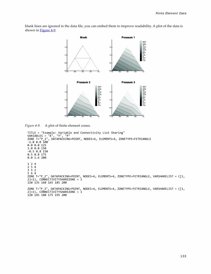
133
Finite Element Data
blank lines are ignored in the data file, you can embed them to improve readability. A plot of the data is shown in Figure 4-9.
Figure 4-9. A plot of finite element zones.
TITLE = "Example: Variable and Connectivity List Sharing"VARIABLES = "X", "Y", "P"ZONE T="P_1", DATAPACKING=POINT, NODES=6, ELEMENTS=4, ZONETYPE=FETRIANGLE-1.0 0.0 1000.0 0.0 1251.0 0.0 150-0.5 0.8 1500.5 0.8 1750.0 1.6 200
1 2 42 5 43 5 25 6 4ZONE T="P_2", DATAPACKING=POINT, NODES=6, ELEMENTS=4, ZONETYPE=FETRIANGLE, VARSHARELIST = ([1, 2]=1), CONNECTIVITYSHAREZONE = 1110 135 160 165 185 200
ZONE T="P_3", DATAPACKING=POINT, NODES=6, ELEMENTS=4, ZONETYPE=FETRIANGLE, VARSHARELIST = ([1, 2]=1), CONNECTIVITYSHAREZONE = 1120 145 180 175 195 200

134
4 - 5.2 Finite Element Data Set ExamplesCreating a finite element data set is generally more complicated than creating a similar-sized ordered data set1. In addition to specifying all the data points, you must also specify the connectivity list. Consider the data shown in Table 4 - 1.
You can create a POINT Tecplot 360 data file for this data set as follows (a 2D mesh plot of this data set is shown in Figure 4-10):
TITLE = "Example: 2D Finite Element Data"VARIABLES = "X", "Y", "P", "T"ZONE NODES=8, ELEMENTS=4, DATAPACKING=POINT, ZONETYPE=FEQUADRILATERAL0.0 1.0 100.0 1.61.0 1.0 150.0 1.53.0 1.0 300.0 2.00.0 0.0 50.0 1.01.0 0.0 100.0 1.43.0 0.0 200.0 2.4.0 0.0 400.0 3.02.0 2.0 280.0 1.91 2 5 42 3 6 56 7 3 33 2 8 8
Figure 4-10. A mesh plot of 2D finite element data.
The ZONE record describes completely the form and format of the data set: there are eight nodes, indicated by the parameter NODES=8; four elements, indicated by the parameter ELEMENTS=4, and the elements are all quadrilaterals, as indicated by the parameter ZONETYPE=FEQUADRILATERAL.
1. Background information for FE data sets is provided in Section “Indexing Cell-centered Ordered Data” in the User’s Manual.
Node X Y P T
A 0.0 1.0 100.0 1.6
B 1.0 1.0 150.0 1.5
C 3.0 1.0 300.0 2.0
D 0.0 0.0 50.0 1.0
E 1.0 0.0 100.0 1.4
F 3.0 0.0 200.0 2.2
G 4.0 0.0 400.0 3.0
H 2.0 2.0 280.0 1.9Table 4 - 1: finite element Data

135
Finite Element Data
The same data file can be written more compactly in BLOCK format as follows:
TITLE = "Example: 2D Finite Element Data"VARIABLES = "X", "Y", "P", "T"ZONE NODES=8, ELEMENTS=4, DATAPACKING=BLOCK, ZONETYPE=FEQUADRILATERAL0.0 1.0 3.0 0.0 1.0 3.0 4.0 2.01.0 1.0 1.0 0.0 0.0 0.0 0.0 2.0100.0 150.0 300.0 50.0 100.0 200.0 400.0 280.01.6 1.5 2.0 1.0 1.4 2.2 3.0 1.91 2 5 42 3 6 56 7 3 33 2 8 8
In BLOCK format, all values for a single variable are written in a single block. The length of the block is the number of data points in the zone. In POINT format, all variables for a single data point are written in a block, with the length of the block equal to the number of variables.
You can change the connectivity list to obtain a different mesh for the same data points. In the above example, substituting the following connectivity list yields the five-element mesh shown in Figure 4-11. (You must also change the ELEMENTS parameter in the zone control line to specify five elements.)
Figure 4-11. Finite element data of Figure 4-10 with a different connectivity list
1 2 4 44 2 3 55 3 6 66 7 3 33 2 8 8
The connectivity list is the same for both POINT and BLOCK formats.

136
Two-Dimensional Field PlotsA 2D finite element data file is shown below:.
Figure 4-12. A 2D field plot.
TITLE = "Example: 2D Finite Element Data"VARIABLES = "X", "Y", "P", "T"ZONE NODES=8, ELEMENTS=4, DATAPACKING=POINT, ZONETYPE=FEQUADRILATERAL0.0 1.0 75.0 1.61.0 1.0 100.0 1.53.0 1.0 300.0 2.00.0 0.0 50.0 1.01.0 0.0 100.0 1.43.0 0.0 200.0 2.24.0 0.0 400.0 3.02.0 2.0 280.0 1.91 2 5 42 3 6 56 7 3 33 2 8 8
The above finite element data file has eight nodes (the first eight rows of the zone) and four elements (the last four rows of the zone). Each row in the node matrix represents a given node. Each column in the row matrix corresponds to the value of each variable at a given node. The order of the variables definition correlates to the order the variables are named in the data set, i.e. for node one, X = 0.0, Y=1.0, P = 75.0 and T = 1.6. The element matrix defines the connectivity of the nodes, i.e. element one is composed of nodes one, two, five and four.
Please refer to Chapter 3: “Data Structure” in the User’s Manual for information on ordered and FE data sets.

137
Finite Element Data
Triangle Data in BLOCK Format ExampleAn example of triangle element type finite element data is listed below. There are two variables (X, Y) and five data points. This data set is plotted in Figure 4-13. Each data point is labeled with its node number.
Figure 4-13. A finite element triangle data set.
In this example, each column of the data section corresponds to a node and each row to a variable. Each row of the connectivity list corresponds to a triangular element and each column specifies a node number.
VARIABLES = "X", "Y"ZONE NODES=5, ELEMENTS=3, DATAPACKING=BLOCK, ZONETYPE=FETRIANGLE1.0 2.0 2.5 3.5 4.01.0 3.0 1.0 5.0 1.01 2 33 2 43 5 4
FORTRAN CodeThis FORTRAN code creates triangle element type finite element data in BLOCK format:
INTEGER VAR . . WRITE (*,*) ´ZONE DATAPACKING=BLOCK, ZONETYPE=FETRIANGLE,NODES=´,NNODES,&´ ,ELEMENTS=´,NELEM DO 1 VAR=1,NUMVAR DO 1 NODES=1,NNODES WRITE(*,*) VARRAY(VAR,NODES)1 CONTINUE DO 2 M=1,NELEM DO 2 L=1,3 WRITE (*,*) NDCNCT(M,L)2 CONTINUE
Finite Element Zone Node Variable Parameters ExampleThe node variable parameter allows setting of the connectivity to match the value of the selected node variable. In the example below, the files appear to be identical in Tecplot 360, although the connectivity list has changed to reflect the values of the node order. Notice that the index value of the nodes is not changed by the node variable value.
The original data set:
TITLE = "Data with original node ordering"

138
VARIABLES = "X" "Y"ZONE T="Triangulation" NODES=6, ELEMENTS=5,DATAPACKING=POINT, ZONETYPE=FETRIANGLEDT=(SINGLE SINGLE) 2.00E+000 3.00E+000 2.20E+000 3.10E+000 3.10E+000 4.20E+000 2.80E+000 3.50E+000 2.40E+000 2.10E+000 4.30E+000 3.20E+000 1 2 5 6 4 3 5 4 6 2 3 4 5 2 4
The data set with the nodes re-ordered for connectivity:
TITLE = "Data with modified node ordering"VARIABLES = "X" "Y" "Node-Order"ZONE T="Triangulation" NODES=6, NV = 3, ELEMENTS=5,DATAPACKING=POINT, ZONETYPE=FETRIANGLEDT=(SINGLE SINGLE) 2.00E+000 3.00E+000 5 2.20E+000 3.10E+000 4 3.10E+000 4.20E+000 1 2.80E+000 3.50E+000 2 2.40E+000 2.10E+000 6 4.30E+000 3.20E+000 3 5 4 6 3 2 1 6 2 3 4 1 2 6 4 2
FE surface dataFinite element surface data specify node locations in three dimensions. Consider the data in Table 4 - 2. Locations are listed for eleven nodes, each having only the three spatial variables X, Y, and Z. We would like to create an finite element surface zone with this data set, where some of the elements are triangles and some are quadrilaterals. All the elements could be organized into one zone of element type Quadrilateral. However, as an illustration of creating 3D surface data, create three zones: one triangular, one quadrilateral, and one a mixture (using quadrilaterals with repeated nodes for the triangles).
X Y Z
0.0 0.0 1.0
0.0 0.0 -2.0
1.0 0.0 -2.0
1.0 1.0 0.0
1.0 1.0 -1.0
1.0 -1.0 0.0
1.0 -1.0 -1.0
-1.0 1.0 0.0
-1.0 1.0 -1.0Table 4 - 2: Data set with eleven nodes and three variables.

139
Finite Element Data
A Tecplot 360 data file for the data in Table 4 - 2 is shown below in POINT format and plotted in Figure 4-14:
TITLE = "Example: 3D FE-SURFACE ZONES"VARIABLES = "X", "Y", "Z"ZONE T="TRIANGLES", NODES=5, ELEMENTS=4, DATAPACKING=POINT, ZONETYPE=FETRIANGLE0.0 0.0 1.0-1.0 -1.0 0.0-1.0 1.0 0.01.0 1.0 0.01.0 -1.0 0.01 2 31 3 41 4 51 5 2ZONE T="PURE-QUADS", NODES=8, ELEMENTS=4, DATAPACKING=POINT,
ZONETYPE=FEQUADRILATERAL-1.0 -1.0 0.0-1.0 1.0 0.01.0 1.0 0.01.0 -1.0 0.0-1.0 -1.0 -1.0-1.0 1.0 -1.01.0 1.0 -1.01.0 -1.0 -1.01 5 6 22 6 7 33 7 8 44 8 5 1ZONE T="MIXED", NODES=6, ELEMENTS=4, DATAPACKING=POINT, ZONETYPE=FEQUADRILATERAL-1.0 -1.0 -1.0-1.0 1.0 -1.01.0 1.0 -1.01.0 -1.0 -1.00.0 0.0 -2.01.0 0.0 -2.01 5 2 22 5 6 33 4 6 64 1 5 6
-1.0 -1.0 0.0
-1.0 -1.0 -1.0
X Y Z
Table 4 - 2: Data set with eleven nodes and three variables.

140
Figure 4-14. Three-dimensional mesh plot of finite element surface data.
FE Volume Data FilesFinite element volume data in Tecplot 360 is constructed from either tetrahedra having four nodes or bricks having eight nodes. Bricks are more flexible, because they can be used (through the use of repeated nodes in the connectivity list) to construct elements with fewer than eight nodes and combine those elements with bricks in a single zone.
Finite Element Volume - Brick Data SetAs a simple example of finite element volume brick data, consider the data in Table 4 - 3. The data can be divided into five brick elements, each of which is defined by eight nodes.
X Y Z Temperature
0.0 0.0 0.0 9.5
1.0 1.0 0.0 14.5
1.0 0.0 0.0 15.0
1.0 1.0 1.0 16.0
1.0 0.0 1.0 15.5
2.0 2.0 0.0 17.0
2.0 1.0 0.0 17.0
2.0 0.0 0.0 17.5
2.0 2.0 1.0 18.5
2.0 1.0 1.0 20.0
2.0 0.0 1.0 17.5
2.0 2.0 2.0 18.0Table 4 - 3: Finite Element Volume - Brick Data Set. Data with 14 nodes and four variables.

141
Finite Element Data
In each element’s connectivity list, Tecplot 360 draws connections from each node to three other nodes. You can think of the first four nodes in the element as the “bottom” layer of the brick, and the second four nodes as the “top.” Within the bottom or top layer, nodes are connected cyclically (1-2-3-4-1; 5-6-7-8-5); the layers are connected by connecting corresponding nodes (1-5; 2-6; 3-7; 4-8). Figure 4-8 illustrates this basic connectivity. When you are creating your own connectivity lists for brick elements, you must keep this basic connectivity in mind, particularly when using duplicate nodes to create pyramids and wedges. Tecplot 360 lets you create elements that violate this basic connectivity, but the result will probably not be what you want.
The data file in POINT format is shown below:
TITLE = "Example: FE-Volume Brick Data"VARIABLES = "X", "Y", "Z", "Temperature"ZONE NODES=14, ELEMENTS=5, DATAPACKING=POINT, ZONETYPE=FEBRICK0.0 0.0 0.0 9.51.0 1.0 0.0 14.51.0 0.0 0.0 15.01.0 1.0 1.0 16.01.0 0.0 1.0 15.52.0 2.0 0.0 17.02.0 1.0 0.0 17.02.0 0.0 0.0 17.52.0 2.0 1.0 18.52.0 1.0 1.0 20.02.0 0.0 1.0 17.52.0 2.0 2.0 18.02.0 1.0 2.0 17.52.0 0.0 2.0 16.51 1 1 1 2 4 5 32 4 5 3 7 10 11 84 4 5 5 10 13 14 114 4 4 4 9 12 13 102 2 4 4 7 6 9 10
The same data in BLOCK format is shown below:
TITLE = "Example: FE-Volume Brick Data"VARIABLES = "X", "Y", "Z", "Temperature"ZONE NODES=14, ELEMENTS=5, DATAPACKING=BLOCK, ZONETYPE=FEBRICK0.0 1.0 1.0 1.0 1.0 2.0 2.0 2.0 2.0 2.0 2.0 2.0 2.0 2.00.0 1.0 0.0 1.0 0.0 2.0 1.0 0.0 2.0 1.0 0.0 2.0 1.0 0.00.0 0.0 0.0 1.0 1.0 0.0 0.0 0.0 1.0 1.0 1.0 2.0 2.0 2.09.5 14.5 15.0 16.0 15.5 17.0 17.017.5 18.5 20.0 17.5 18.0 17.5 16.51 1 1 1 2 4 5 32 4 5 3 7 10 11 84 4 5 5 10 13 14 114 4 4 4 9 12 13 102 2 4 4 7 6 9 10
2.0 1.0 2.0 17.5
2.0 0.0 2.0 16.5
X Y Z Temperature
Table 4 - 3: Finite Element Volume - Brick Data Set. Data with 14 nodes and four variables.

142
Figure 4-15 shows the resulting mesh plot from the data set listed in this section.
Figure 4-15. A finite element brick zone.
Finite Element Volume - Tetrahedral Data SetAs a simple example of a finite element volume data set using tetrahedral elements, consider the data in Table 4 - 4. The data set consists of thirteen nodes, with seven variables. The nodes are to be connected to form twenty tetrahedral elements, each with four nodes.
The data file in POINT format for the data in Table 4 - 4 is shown below, and plotted in Figure 4-16:
TITLE = "Example: FE-Volume Tetrahedral Data"VARIABLES = "X", "Y", "Z", "C", "U", "V", "W"ZONE NODES=13, ELEMENTS=20, DATAPACKING=POINT, ZONETYPE=FETETRAHEDRON0 0 -95 -1 1 0 80 85 -42 0 -85 -3 981 26 -42 2 -22 80 8
X Y Z C U V W
0 0 -95 -1 1 0 8
0 85 -42 0 -5 -3 9
81 26 -42 2 -22 80 8
50 -69 -42 -6 72 52 9
-50 -69 -42 14 67 -48 9
-81 26 -2 20 -30 -82 9
0 0 0 1 -2 -5 10
50 69 43 14 -68 48 11
81 -26 43 20 31 82 11
0 -85 43 0 84 -3 10
-81 -26 43 2 21 -80 11
-50 69 43 -6 -71 -51 11
0 0 96 1 0 -1 12Table 4 - 4: Finite Element Volume - Tetrahedral data set with 13 nodes and seven variables.
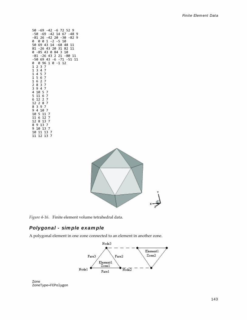
143
Finite Element Data
50 -69 -42 -6 72 52 9-50 -69 -42 14 67 -48 9-81 26 -42 20 -30 -82 90 0 0 1 -2 -5 1050 69 43 14 -68 48 1181 -26 43 20 31 82 110 -85 43 0 84 3 10-81 -26 43 2 21 -80 11-50 69 43 -6 -71 -51 110 0 96 1 0 -1 121 2 3 71 3 4 71 4 5 71 5 6 71 6 2 72 8 3 73 9 4 74 10 5 75 11 6 76 12 2 712 2 8 78 3 9 79 4 10 710 5 11 711 6 12 712 8 13 78 9 13 79 10 13 710 11 13 711 12 13 7
Figure 4-16. Finite element volume tetrahedral data.
Polygonal - simple exampleA polygonal element in one zone connected to an element in another zone.
ZoneZoneType=FEPolygon

144
Nodes=3Faces=3Elements=1NumConnectedBoundaryFaces=2TotalNumBoundaryConnections=1
…variable values in block format…
#face nodes1 22 33 1#left elements1 1 1#right elements (negative indicates boundary connections)0 -1 0#boundary connection counts1#boundary connection elements1#boundary connection zones2
Polyhedral - complex exampleA single tetrahedron bounded on face two by zone two (elements 13 and 14) and on face three by zone three (element 11).
ZoneZoneType=FEPolyhedronNodes=4Faces=4Elements=1TotalNumFaceNodes=12NumConnectedBoundaryFaces=2TotalNumBoundaryConnections=3
…variable values in block format…
#node count per face3 3 3 3#face nodes1 2 31 4 22 4 33 4 1#left elements (negative indicates boundary connection)0 -1 -2 0#right elements1 1 1 1#boundary connection counts2 1#boundary connection elements13 14 11#boundary connection zones2 2 3
4 - 6 ASCII Data File Conversion to BinaryAlthough Tecplot 360 can read and write ASCII or binary data files, binary data files are more compact and are read into Tecplot 360 much more quickly. Even if you write ASCII files, for best performance, we recommend that you convert your data files to binary as a post-processing step, before interactive visualization.
In the bin folder of your Tecplot 360 distribution you will find Preplot, which converts ASCII to binary data files. You can also use Preplot to debug ASCII data files that Tecplot 360 cannot read.

145
ASCII Data File Conversion to Binary
4 - 6.1 Preplot OptionsTo use Preplot, type the following command from the UNIX shell prompt, from a DOS prompt, or using the Run command on Windows platforms:
preplot infile [outfile] [options]
where infile is the name of the ASCII data file, outfile is an optional name for the binary data file created by Preplot, and options is a set of options from the standard set of Preplot options. If outfile is not specified, the binary data file has the same base name as the infile with a .plt extension. You may use a minus sign (“-”) in place of either the infile or outfile to specify standard input or standard output, respectively.
Any or all of -iset, -jset, and -kset can be set for each zone, but only one of each per zone.
For the standard set of preplot options, see Section B - 3 “Preplot” in the User’s Manual.
4 - 6.2 Preplot ExamplesIf you have an ASCII file named dset.dat, you can create a binary data file called dset.plt with the following Preplot command:
preplot dset.dat dset.plt
By default, Preplot looks for files with the .dat extension, and creates binary files with the .plt extension. Thus, either of the following commands is equivalent to the above command:
preplot dsetpreplot dset.dat
Preplot checks the input ASCII data file for errors such as illegal format, numbers too small or too large, the wrong number of values in a data block, and illegal finite element node numbers. If Preplot finds an error, it issues a message displaying the line and column where the error was first noticed. This is only an indication of where the error was detected; the actual error may be in the preceding columns or lines.
If Preplot encounters an error, you may want to set the debug option to get more information about the events leading up to the error:
preplot dset.dat -d
You can set the flag to -d2, or -d3, or -d4, and so forth, to obtain more detailed information.
In the following Preplot command line, the number of points that are written to the binary data file dset.plt is less than the number of points in the input file dset.dat:
preplot dset.dat -iset 3,6,34,2 -jset 3,1,21,1 -iset 4,4,44,5
For zone three, Preplot outputs data points with I-index starting at six and ending at 34, skipping every other one, and J-index starting at one and ending at 21. For zone four, Preplot outputs data points with the I-index starting at four, ending at 44, and skipping by five.
In the following Preplot command line, every other point in the I-, J-, and K-directions is written to the binary data file:
preplot dset.dat -iset ,,,2 -jset ,,,2 -kset ,,,2
The zone, start, and end parameters are not specified, so all zones are used, starting with index one, and ending with the maximum index. The overall effect is to reduce the number of data points by a factor of about eight.

146
147
5
Glossary
The following terms are used throughout the Data Format Guide and are included here for your reference.
2D Plotting in two dimensions. Line plots of one or more variables (XY and Polar Line plots) are not considered 2D.
2D Cartesian Plot A plot of some variable by location on a single plane using two axes.
3D Plotting in three dimensions. Three-dimensional plotting can be subdivided into 3D surface and 3D volume.
3D Cartesian Plot A plot displaying a 3D scattering of points, surfaces, or volumes using three orthogonal axes.
3D Surface Three-dimensional plotting confined to a surface. For example, the surface of a wing.
3D Volume Three-dimensional plotting of data that includes interior data points of a volume, as well as those on the surface. For example, the vector field around a wing.
Active Zone A zone that is displayed in the current plot, as determined in the Zone Style dialog.
ASCII Data File A data file composed of human-readable statements and numbers using ASCII characters.
Auxiliary Data Metadata attached to zones, data sets, and frames.
Binary Data File A data file composed of machine-readable data. This type of file is created by converting ASCII data files with Preplot, or by directly creating them from an application.
Block A data file format in which the data is listed by variable. All the point values of the first variable are listed first, then all the point values of the second variable, and so forth.
Boundary Cell Faces
A set of un-blanked cell faces in a 3D volume zone which have only one neighboring volume cell. In contrast, interior cell faces have two neighboring volume cells, one on either side, which share the face. For an IJK-ordered zone the boundary cell faces are on the exterior of the zone. That is, the first and last I-planes, the first and last J-planes, and the first and last K-planes. For a finite element 3D volume zone, boundary cell faces are on the exterior of the zone and the surface of any voids within the zone.

148
Brick An element type of finite element volume data composed of eight node points arranged in a hexahedron-like format. This element type is used in 3D volume plotting.
Cell Either an element of finite element data, or the space contained by one increment of each index of IJ- or IJK-ordered data.
Cell-Centered Val-ues Values located at the center of the cell (assumed to be the centroid).
Connectivity List The portion of a finite element data file which defines the elements or cells by listing the relationships between points. The number of points per cell is determined by the element type.
Custom Labels Text strings contained within a data file or text geometry file which define labels for your axes or contour table. You may select Custom Labels anywhere you can choose a number format, the result is the text strings in place of numbers. The maximum length of a custom label is 1024 characters.
Data File A file that contains data used for plotting in Tecplot.
Data Format The type of zone data as specified by the format parameter in a Tecplot data file, such as: BLOCK or POINT.
Data Loader A Tecplot add-on which allows you to read non-Tecplot data files.
Data Point An XYZ-point at which field variables are defined.
Data Set A set of one or more zones. A data set may be plotted in one or more frames. However, a single frame may only plot one data set. A data set may be created by loading one or more data files.
Element Type The form of individual elements in a finite element zone. There are four types of cell-based finite element zones: Triangle and Quadrilateral (finite element surface types), and Tetrahedron and Brick (finite element volume types). For cell-based finite elements, the element type of a zone determines the number of nodes per element and their orientation within an element.There are two types of face-based finite element zones: polygonal (2D) and polyhedral (3D). For face-based elements, the number of nodes per element is variable.
FE An abbreviation for finite element, a common means of arranging data for calculations. (Often referred to as “unordered” or “unstructured”.)
FE Surface A finite element zone of the element type Triangle, Quadrilateral, Polygon. These zones are used for 2D and 3D surface plots.
FE Volume A finite element zone of the element type Tetrahedron, Brick, Polyhedron. These zones are used for 3D volume plots.
Field Map A collection of zones for 2D and 3D field plots. A common style can be easily applied to all zones in the selection.
Field Plot Includes 2D Cartesian and 3D Cartesian plot types. Generally used to display the spacial relationship of data. Mesh, Contour, Vector, Scatter and Shade are all considered field plots. XY and Polar Line plots and the Sketch plot type are not field plots.
Finite Element A type of data point ordering. Data is arranged by listing the data points (called nodes), and then listing their relationships (called elements). The element type of the zone determines the number of nodes which are contained in each element, as well as the exact relationship of nodes within an element. There are several different element types supported by Tecplot: Triangle,Quadrilateral,Tetrahedron, Brick, Polygonal and Polyhedral. See also: Connectivity List and Node

149
I-Ordered A type of data point ordering where each point is listed one at a time (that is, by one index). Used mainly in XY-plots. In 2D or 3D, this type of data point ordering is sometimes called irregular, and is only useful for scatter plots, or for interpolating into 2D, 3D surface, or 3D volume zones. (This type of data can also be used for 2D or 3D vector plots if streamtraces are not required.)
IJ-Ordered A type of data point ordering where the points are arranged in a 2D array used for 2D and 3D surface plotting.
IJK-Blanking A feature to include or exclude portions of an IJK-ordered zone based on index ranges.
IJK-Ordered A type of data ordering where the points are arranged in a 3D array. Used for 3D volume plotting as well as 2D and 3D surface plotting.
I-Plane In an ordered zone, the connected surface of all points with a constant I-index. In reality, I-planes may be cylinders, spheres, or any other shape.
Irregular Data Points which have no order, or at least no order which can be easily converted to IJ- or IJK-ordering.
J-Plane In an ordered zone, the connected surface of all points with a constant J-index. In reality, J-planes may be cylinders, spheres, or any other shape.
K-Plane In an IJK-ordered zone, the connected surface of all points with a constant K-index. In reality, K-planes may be cylinders, spheres, or any other shape.
Macro A file containing a list of instructions, called macro commands, which can duplicate virtually any action performed in Tecplot.
Macro Command An instruction given to Tecplot in a macro file. Macro commands always start with a dollar sign and then an exclamation mark. For example, $!Redraw refreshes a plot view.
Macro File A file which contains a series of macro commands. Macro files are run from the command line, or through the Play option of the Macro sub-menu of the File menu.
Macro Function A self-contained macro sub-routine.
Macro Variable A holding place for numeric values in a macro file. There are two types of macro variables: user-defined (you set and retrieve the value), or internal (Tecplot sets the value and you may retrieve it).
No Neighboring Element
In polyhedral/polygonal fe data sets, the term “no neighboring element” refers to a face that does not have a neighboring element on either its right or left side.
Node A point in finite element data.
Number Format The style of numbers to display for a data or axis label; exponent, integer, float, and so forth.
Ordered Data A type of data point organization which consists of a parameterized series of points. There are seven types of ordered data: I-, J-, K-, IJ-, JK-, IK-, and IJK-ordered. I-, IJ-, and IJK-ordered are the most common.
Polygonal A 2D, face-based finite element type. The number of nodes per element is variable. That is, a single polygonal zone may contain triangular, quadrilateral, hexagonal, ..., etc. elements.
Polyhedral A 3D, face-based finite element type. The number of nodes per element is variable. That is, a single polyhedral zone may contain tetrahedral and brick (and others) elements.
Point A data file format for an I-, IJ-, or IJK-ordered zone in which the data is listed by point. All of the variable values for the first data point are listed first, then all the variable values for the second data point, and so forth.
150
Quadrilateral An element type of finite element surface data which is composed of four node points arranged in a quadrilateral. Used in 2D and 3D surface plotting.
Sharing Variable sharing allows a single storage location to be used by more than one party. For example, if the X-variable is shared between zones five and seven only one storage location is created. The storage is not freed by Tecplot until the number of parties accessing the data is reduced to zero. Variables and connectivity information may be shared.
Subzone Loadable A file format (.szplt) introduced in Tecplot 360 EX that allows partial zones (subzones) to be loaded as needed for plots and other operations. In typical use, this significantly improves performance and reduces memory footprint compared to .plt files.
Tetrahedron An element type of finite element volume data which is composed of four node points arranged in a tetrahedron. (Used in 3D volume plotting.)
Triangle An element type of finite element surface data which is composed of three node points arranged in a triangle. (Used in 2D and 3D surface plotting.)
Unordered or Unorganized Data (See Irregular Data.)
Zone A subset of a data set which is assigned certain plot types. Zones may be activated (plotted) or deactivated (not plotted). Each zone has one type of data ordering: I-, IJ-, IJK-, or finite element. Zones are typically used to distinguish different portions of the data. For example, different calculations, experimental versus theoretical results, different time steps, or different types of objects, such as a wing surface versus a vector field around a wing.
Zone Layers One way of displaying a 2D or 3D plot’s data set. The plot is the sum of the active zone layers, which may include mesh, contour, vector, shade, scatter and edge.

151
A
Binary Data File Format
Refer to this section only if you wish to write your own code that writes Tecplot binary-format (.plt) files without utilizing the TecIO library. Otherwise, refer to Section 3 - 1 “Getting Started” for instructions for linking with this library, which is provided at no cost by Tecplot, Inc.
The subzone loadable format (.szplt) is not currently documented because we anticipate the need for changes to the file format in the near future. Furthermore, the format is sufficiently complex that we do not expect application developers finding it worthwhile to undertake writing their own code to output in .szplt format. If you want your application to write subzone loadable files and find the TecIO library insufficient, please contact us.
/*BINARY FILE FORMAT:-----------------------------------------------------------------------The binary data file format (as produced by the preplot) is described below.
The binary datafile has two main sections. A header section and a datasection.
+----------------+ | HEADER SECTION | +----------------+ +---------+ |FLOAT32 | EOHMARKER, value=357.0 +---------+ +----------------+ | DATA SECTION | +----------------+
I. HEADER SECTION
The header section contains: the version number of the file, a title of the file, the names of the variables to be plotted, the descriptions of all zones to be read in and all text and geometry definitions.
i. Magic number, Version number

152
+-----------+ | “#!TDV112”| 8 Bytes, exact characters “#!TDV112”. +-----------+ Version number follows the “V” and consumes the next 3 characters (for example: “V75 “, “V101”).
ii. Integer value of 1. +-----------+ | INT32 | This is used to determine the byte order +-----------+ of the reader, relative to the writer.
iii. Title and variable names. +-----------+ | INT32 | FileType: 0 = FULL, +-----------+ 1 = GRID, 2 = SOLUTION +-----------+ | INT32*N | The TITLE. (See note 1.) +-----------+ +-----------+ | INT32 | Number of variables (NumVar) in the datafile. +-----------+ +-----------+ | INT32*N | Variable names. +-----------+ N = L[1] + L[2] + .... L[NumVar] where: L[i] = length of the ith variable name + 1 (for the terminating 0 value). (See note 1.) iv. Zones +-----------+ | FLOAT32 | Zone marker. Value = 299.0 +-----------+ +-----------+ | INT32*N | Zone name. (See note 1.) +-----------+ N = (length of zone name) + 1. +-----------+ | INT32 | ParentZone: Zero-based zone number within this +-----------+ datafile to which this zone is a child. +-----------+ | INT32 | StrandID: -2 = pending strand ID for assignment +-----------+ by Tecplot -1 = static strand ID 0 <= N < 32700 valid strand ID +-----------+ | FLOAT64 | Solution time. +-----------+ +-----------+ | INT32 | Not used. Set to -1. +-----------+ +-----------+ | INT32 | ZoneType 0=ORDERED, 1=FELINESEG, +-----------+ 2=FETRIANGLE, 3=FEQUADRILATERAL, 4=FETETRAHEDRON, 5=FEBRICK, 6=FEPOLYGON, 7=FEPOLYHEDRON +-----------+ | INT32 | Data packing. +-----------+ 0 = Block 1 = Point +-----------+ | INT32 | Specify Var Location. +-----------+ 0 = Don’t specify, all data is located at the nodes. 1 = Specify if “specify var location” == 1 +-----------+ | INT32*NV | Variable Location (only specify if above is 1). +-----------+ 0 = Node, 1 = Cell Centered (See note 5.) +-----------+

153
| INT32 | Are raw local 1-to-1 face neighbors supplied? +-----------+ (0=FALSE 1=TRUE). These raw values are a compact form of the local 1-to-1 face neighbors. If supplied, Tecplot assumes that the face neighbors are fully specified. As such, it will not perform auto face neighbor assignment. This improves Tecplot’s time to first plot. See the data section below for format details. ORDERED and FELINESEG zones must specify 0 for this value because raw face neighbors are not defined for these zone types. FEPOLYGON and FEPOLYHEDRON zones must specify 0 for this value since face neighbors are defined in the face map for these zone types.
+-----------+ | INT32 | Number of miscellaneous user-defined face +-----------+ neighbor connections (value >= 0). This value is in addition to the face neighbors supplied in the raw section. FEPOLYGON and FEPOLYHEDRON zones must specify 0.
if “number of miscellaneous user-defined face neighbor connections” != 0 +-----------+ | INT32 | User defined face neighbor mode +-----------+ (0=Local 1-to-1, 1=Local 1-to-many, 2=Global 1-to-1, 3=Global 1-to-many) if FE Zone: +-----------+ | INT32 | Indicates if the finite element face neighbors +-----------+ are completely specified by the miscellaneous face neighbors given: (0=NO, 1=YES). If yes, then Tecplot will not perform auto assignment of face neighbors otherwise all faces not specified are considered boundaries. If no, then Tecplot will perform auto-assignment of the face neighbors unless the raw face neighbor array was supplied. This option is not valid for ORDERED zones. if Ordered Zone: +-----------+ | INT32*3 | IMax,JMax,KMax +-----------+
if FE Zone: +-----------+ | INT32 | NumPts +-----------+ if ZoneType is FEPOLYGON or FEPOLYHEDRON: +-----------+ | INT32 | NumFaces +-----------+ +-----------+ | INT32 | Total number of face nodes. For FEPOLYGON +-----------+ zones, this is NumFaces*2. +-----------+ | INT32 | Total number of boundary faces. If any +-----------+ boundary faces exist, include one to represent no neighboring element. +-----------+ | INT32 | Total number of boundary connections. +-----------+ +-----------+ | INT32 | NumElements +-----------+ +-----------+ | INT32*3 | ICellDim,JCellDim, +-----------+ KCellDim (for future use; set to zero)
For all zone types (repeat for each Auxiliary data name/value pair):
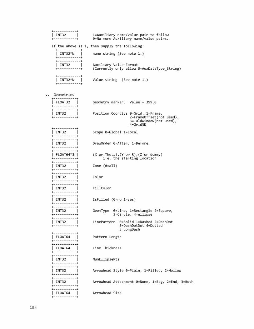
154
+-----------+ | INT32 | 1=Auxiliary name/value pair to follow +-----------+ 0=No more Auxiliary name/value pairs.
If the above is 1, then supply the following: +-----------+ | INT32*N | name string (See note 1.) +-----------+ +-----------+ | INT32 | Auxiliary Value Format +-----------+ (Currently only allow 0=AuxDataType_String) +-----------+ | INT32*N | Value string (See note 1.) +-----------+
v. Geometries +-----------+ | FLOAT32 | Geometry marker. Value = 399.0 +-----------+ +-----------+ | INT32 | Position CoordSys 0=Grid, 1=Frame, +-----------+ 2=FrameOffset(not used), 3= OldWindow(not used), 4=Grid3D +-----------+ | INT32 | Scope 0=Global 1=Local +-----------+ +-----------+ | INT32 | DrawOrder 0=After, 1=Before +-----------+ +-----------+ | FLOAT64*3 | (X or Theta),(Y or R),(Z or dummy) +-----------+ i.e. the starting location +-----------+ | INT32 | Zone (0=all) +-----------+ +-----------+ | INT32 | Color +-----------+ +-----------+ | INT32 | FillColor +-----------+ +-----------+ | INT32 | IsFilled (0=no 1=yes) +-----------+ +-----------+ | INT32 | GeomType 0=Line, 1=Rectangle 2=Square, +-----------+ 3=Circle, 4=ellipse +-----------+ | INT32 | LinePattern 0=Solid 1=Dashed 2=DashDot +-----------+ 3=DashDotDot 4=Dotted 5=LongDash +-----------+ | FLOAT64 | Pattern Length +-----------+ +-----------+ | FLOAT64 | Line Thickness +-----------+ +-----------+ | INT32 | NumEllipsePts +-----------+ +-----------+ | INT32 | Arrowhead Style 0=Plain, 1=Filled, 2=Hollow +-----------+ +-----------+ | INT32 | Arrowhead Attachment 0=None, 1=Beg, 2=End, 3=Both +-----------+ +-----------+ | FLOAT64 | Arrowhead Size +-----------+

155
+-----------+ | FLOAT64 | Arrowhead Angle +-----------+ +-----------+ | IN32*N | Macro Function Command (string: N = Length+1) +-----------+ +-----------+ | INT32 | Polyline Field Data Type +-----------+ 1=Float, 2=Double (GTYPE) +-----------+ | INT32 | Clipping (0=ClipToAxes, 1=ClipToViewport, +-----------+ 2=ClipToFrame)
If the geometry type is line then: +-----------+ | INT32 | Number of polylines +-----------+ +-----------+ | INT32 | Number of points, line 1. +-----------+ +-----------+ | GTYPE*N | X-block geometry points N=NumPts +-----------+ +-----------+ | GTYPE*N | Y-block geometry points N=NumPts +-----------+ +-----------+ | GTYPE*N | Z-block geometry points N=NumPts (Grid3D Only) +-----------+ . . .
If the geometry type is Rectangle then +-----------+ | GTYPE*2 | X and Y offset for far corner of rectangle +-----------+
If the geometry type is Circle then +-----------+ | GTYPE | Radius +-----------+
If the geometry type is Square then +-----------+ | GTYPE | Width +-----------+
If the geometry type is Ellipse then +-----------+ | GTYPE*2 | X and Y Radii +-----------+
vi. Text +-----------+ | FLOAT32 | Text marker. Value=499.0 +-----------+ +-----------+ | INT32 | Position CoordSys 0=Grid, 1=Frame, +-----------+ 2=FrameOffset(not used), 3= OldWindow(not used), 4=Grid3D(New to V10) +-----------+ | INT32 | Scope 0=Global 1=Local +-----------+ +-----------+ | FLOAT64*3 | (X or Theta),(Y or R),(Z or dummy) +-----------+ Starting Location +-----------+ | INT32 | FontType

156
+-----------+ +-----------+ | INT32 | Character Height Units 0=Grid, 1=Frame, 2=Point +-----------+ +-----------+ | FLOAT64 | Height of characters +-----------+ +-----------+ | INT32 | Text Box type 0=NoBox 1=Hollow 2=Filled +-----------+ +-----------+ | FLOAT64 | Text Box Margin +-----------+ +-----------+ | FLOAT64 | Text Box Margin Linewidth +-----------+ +-----------+ | INT32 | Text Box Outline Color +-----------+ +-----------+ | INT32 | Text Box Fill Color +-----------+ +-----------+ | FLOAT64 | Angle +-----------+ +-----------+ | FLOAT64 | Line Spacing +-----------+ +-----------+ | INT32 | Text Anchor. 0=left, 1=center, +-----------+ 2=right, 3=midleft 4=midcenter 5=midright, 6=headleft 7=headcenter 8=headright +-----------+ | INT32 | Zone (0=all) +-----------+ +-----------+ | INT32 | Color +-----------+ +-----------+ | INT32*N | MacroFunctionCommand (string: N = Length + 1) +-----------+ +-----------+ | INT32 | Clipping (0=ClipToAxes, +-----------+ 1=ClipToViewport, 2=ClipToFrame) +-----------+ | INT32*N | Text. N=Text Length+1 +-----------+
vii.CustomLabel +-----------+ | FLOAT32 | CustomLabel Marker; F=599 +-----------+ +-----------+ | INT32 | Number of labels +-----------+ +-----------+ | INT32*N | Text for label 1. (N=length of label + 1) +-----------+ See note 1. +-----------+ | INT32*N | Text for label 2. (N=length of label + 1) +-----------+ See note 1. . . . +-----------+ | INT32*N | Text for label NumLabels. +-----------+ (N=length of label + 1) See note 1.
viii.UserRec +-----------+

157
| FLOAT32 | UserRec Marker; F=699 +-----------+ +-----------+ | INT32*N | Text for UserRec. See note 1. +-----------+
ix. Dataset Auxiliary data. +-----------+ | FLOAT32 | DataSetAux Marker; F=799.0 +-----------+ +-----------+ | INT32*N | Text for Auxiliary “Name”. See note 1. +-----------+ +-----------+ | INT32 | Auxiliary Value Format (Currently only +-----------+ allow 0=AuxDataType_String) +-----------+ | INT32*N | Text for Auxiliary “Value”. See note 1. +-----------+ x. Variable Auxiliary data. +-----------+ | FLOAT32 | VarAux Marker; F=899.0 +-----------+ +-----------+ | INT32*N | Variable number (zero based value) +-----------+ +-----------+ | INT32*N | Text for Auxiliary “Name”. See note 1. +-----------+ +-----------+ | INT32 | Auxiliary Value Format (Currently only +-----------+ allow 0=AuxDataType_String) +-----------+ | INT32*N | Text for Auxiliary “Value”. See note 1. +-----------+
II. DATA SECTION (don’t forget to separate the header from the data with an EOHMARKER). The data section contains all of the data associated with the zone definitions in the header.
i. For both ordered and fe zones: +-----------+ | FLOAT32 | Zone marker Value = 299.0 +-----------+ +-----------+ | INT32*N | Variable data format, N=Total number of vars +-----------+ 1=Float, 2=Double, 3=LongInt, 4=ShortInt, 5=Byte, 6=Bit +-----------+ | INT32 | Has passive variables: 0 = no, 1 = yes. +-----------+ if “has passive variables” != 0 +-----------+ | INT32*NV | Is variable passive: 0 = no, 1 = yes +-----------+ (Omit entirely if “Has passive variables” is 0). +-----------+ | INT32 | Has variable sharing 0 = no, 1 = yes. +-----------+ if “has variable sharing” != 0 +-----------+ | INT32*NV | Zero based zone number to share variable with +-----------+ (relative to this datafile). (-1 = no sharing). (Omit entirely if “Has variable sharing” is 0). +-----------+ | INT32 | Zero based zone number to share connectivity +-----------+ list with (-1 = no sharing). FEPOLYGON and FEPOLYHEDRON zones use this zone number to share face map data.
Compressed list of min/max pairs for each non-shared and non-passive variable. For each non-shared and non-passive variable (as specified

158
above): +-----------+ | FLOAT64 | Min value +-----------+ +-----------+ | FLOAT64 | Max value +-----------+ +-----------+ | xxxxxxxxxx| Zone Data. Each variable is in data format as +-----------+ specified above.
ii. specific to ordered zones if “zone number to share connectivity list with” == -1 && “num of misc. user defined face neighbor connections” != 0 +-----------+ | INT32*N | Face neighbor connections. +-----------+ N = (number of miscellaneous user defined face neighbor connections) * P (See note 5 below).
iii. specific to fe zones if ZoneType is NOT FEPOLYGON or FEPOLYHEDRON: if “zone number to share connectivity lists with” == -1 +-----------+ | INT32*N | Zone Connectivity Data N=L*JMax +-----------+ (see note 2 below ). if “zone number to share connectivity lists with” == -1 && “raw local 1-to-1 face neighbors are supplied” +-----------+ | INT32*N | Raw local 1-to-1 face neighbor array. +-----------+ N = (NumElements * NumFacesPerElement) (See note 3 below). if “zone number to share connectivity lists with” == -1 && “num of misc. user defined face neighbor connections” != 0 +-----------+ | INT32*N | Face neighbor connections. +-----------+ N = (number of miscellaneous user defined face neighbor connections) * P (See note 4 below).
if ZoneType is FEPOLYGON or FEPOLYHEDRON: if “zone number to share face map data with” == -1 +-----------+ | INT32*F | Face node offsets into the face nodes array +-----------+ below. Does not exist for FEPOLYGON zones. F = NumFaces+1. +-----------+ | INT32*FN | Face nodes array containing the node numbers +-----------+ for all nodes in all faces. FN = total number of face nodes. +-----------+ | INT32*F | Elements on the left side of all faces. +-----------+ Boundary faces use a negative value which is the negated offset into the face boundary connection offsets array. A value of “-1” indicates there is no left element. F = NumFaces.
+-----------+ | INT32*F | Elements on the right side of all faces. See +-----------+ description of left elements above for more details. F = NumFaces.
if “total number of boundary faces” != 0 +-----------+ | INT32*NBF | Boundary face connection offsets into the +-----------+ boundary face connecion elements array and

159
the boundary face connection zones array. The number of elements for a face (F) is determined by offset[-o] - offset[-o-1] where ‘o’ is the negative value from either the left or right elements arrays above. Offset[0] = 0. Offset[1] = 0 so that -1 as the left or right element always indicates no neighboring element. If the number of elements is 0, then there is no neighboring element. NBF = total number of boundary faces + 1.
+-----------+ | INT32*NBI | Boundary face connection elements. A value of +-----------+ “-1” indicates there is no element on part of the face. NBI = total number of boundary connections.
+-----------+ | INT32*NBI | Boundary face connection zones. A value of +-----------+ “-1” indicates the current zone. NBI = total number of boundary connections.
NOTES:
1. All character data is represented by INT32 values.
Example: The letter “A” has an ASCII value of 65. The WORD written to the data file for the letter “A” is then 65. In fortran this could be done by doing the following:
Integer*32 I . . I = ICHAR(‘A’);
WRITE(10) I
All character strings are null terminated (i.e. terminated by a zero value)
2. This represents JMax sets of adjacency zero based indices where each set contains L values and L is 2 for LINESEGS 3 for TRIANGLES 4 for QUADRILATERALS 4 for TETRAHEDRONS 8 for BRICKS
3. The raw face neighbor array is dimensioned by (number of elements for the zone) times (the number of faces per element), where each member of the array holds the zero-based element neighbor of that face. A boundary face is one that has no neighboring element and is represented by a -1. Faces should only be neighbors if they logically share nodes and they should be reciprocal.
4. FaceNeighbor Mode # values Data --------------------------------------------------------------------- LocalOneToOne 3 cz,fz,cz LocalOneToMany nz+4 cz,fz,oz,nz,cz1,cz2,...,czn GlobalOneToOne 4 cz,fz,ZZ,CZ GlobalOneToMany 2*nz+4 cz,fz,oz,nz,ZZ1,CZ1,ZZ2,CZ2,...,ZZn,CZn Where: cz = cell in current zone (zero based) fz = face of cell in current zone (zero based) oz = face obscuration flag (only applies to one-to-many):

160
0 = face partially obscured 1 = face entirely obscured nz = number of cell or zone/cell associations (only applies to one-to-many) ZZ = remote Zone (zero based) CZ = cell in remote zone (zero based) cz,fz combinations must be unique and multiple entries are not allowed. Additionally, Tecplot assumes that with the one-to-one face neighbor modes, a supplied cell face is entirely obscured by its neighbor. With one-to-many, the obscuration flag must be supplied. Face neighbors that are not supplied are run through Tecplot’s auto face neighbor generator (FE only).
5. Cell centered variable (DATA SECTION) To make reading of cell centered binary data efficient, Tecplot stores IMax*JMax*KMax numbers of cell centered values, where IMax, JMax, and KMax represent the number of points in the I, J, and K directions. Therefore extra zero values (ghost values) are written to the data file for the slowest moving indices. For example, if your data’s IJK dimensions are 2x3x2, a cell-centered variable will have 1x2x1 (i.e. (I-1)x(J-1)x(K-1)) significant values. However, 2x3x2 values must be written out because it must include the ghost values. Assume that the two significant cell-centered values are 1.5 and 12.5. The ghost values will be output with a zero value.
So if the zone was dimensioned 2x3x2 its cell centered variable would be represented as follows: 1.5 0.0 12.5 0.0 0.0 0.0 0.0 0.0 0.0 0.0 0.0 0.0
If the zone was dimensioned 3x2x2 its cell centered variable would be represented as follows: 1.5 12.5 0.0 0.0 0.0 0.0 0.0 0.0 0.0 0.0 0.0 0.0
and if the zone was dimensioned 2x2x3 its cell centered variable would be represented as follows: 1.5 0.0 0.0 0.0 12.5 0.0 0.0 0.0 0.0 0.0 0.0 0.0
For large variables the wasted space is less significant that it is for the small example above.-----------------------------------------------------------------------*/
161
IndexAAnchor
text position 118ASCII Data
conversion to binary 105, 144Custom Label Record 122File Format 106–124finite-element data 130–144Geometry Record 119–122ordered data 124–130parameters 123syntax 112Text Record 116–119Zone Record 107–116
ASCII formatsyntax 105
Auxiliary Data 23, 110variable auxiliary data 45, 123zone auxiliary data 46
Axis Labels 35
BBinary Data
byte order 29conversion from ASCII 105, 144File Format 151–160geometry creation 29text record 42user record 45
Binary filesdebugging 20writing to multiple 22, 28writing to multiple, example 99
Block Data 111Boundary Connection 52Boundary Face 52Boundary Map 116Brick cells 131Byte order 29
CCell-centered 15Cell-centered Data 25, 111Cell-centered data 15Connected Boundary Face 52Connectivity list 113
cell-based finite elements 36, 37face-based finite elements 37sharing 110, 116
Custom Label RecordASCII data 122binary data 35
DData
cell-centered 15FE Volume 14nodal 15
Data Arrangement 25Data conversion 105, 144
Data File FormatASCII 106–124binary 151–160
Data structurefinite-element 12ordered data 12
Data Types 111
EElements
finite element zone types to specify 108EOF 26Examples
ASCIIauxiliary data 123finite-element 134–144Geometry 121ordered data 125–130Text Record 119
BinaryFace Neighbors 56IJ-ordered 96polygonal data 63polyhedral zones 68, 80, 93text record 102
FFace Neighbors 113, 115
data 26example 56mode 114polyhedral zones 54right-hand rule 54scope 114
Face Numberingcell-based finite elements 114
Facemap data 37, 115polyhedral zones 53
Facesface-based finite element zone types to specify 108
FE datasee Finite-element
FE-line 14FE-surface 14FE-volume 14File
grid file 35shared grid 35solution file 35
File FormatASCII 106–124Binary Data 151–160
File Header 106Finite-element 12
FE-line 14FE-surface 14FE-volume 14volume data 14
Finite-element dataASCII format 130–144boundary map 116bricks 131connectivity list 36, 37, 113face neighbors 26

INDEX
162
face numbering (cell-based) 114facemap 115line segments 130polygons 131polyhedra 131polyhedral format 37quadrilaterals 131tetrahedron 131triangles 131
Full file 35Function reference
TecIO library 23–51Function sequence
binary files 21
GGeometry Record
ASCII data 119–122binary
syntax 29data (ASCII) 120origin positions 33
Global one-to-many 114Global one-to-one 114Grid
sharing 35Grid File 35
HHeader
file header 106zone header 47
IIrregular data 124
LLabels, custom
binary data 35Legend text 35Line Segments 130Local one-to-many 114Local one-to-one 114
MMetadata, see Auxiliary Data
NNeighboring elements 115Nodal 15Nodal Data 25, 111Nodal data 15Nodes
finite element zone types to specify 108
OOrdered Data 124–130
Example (binary) 96Examples
2D Field Plot 1303D Field Plot 130IJK-ordered 127IJ-ordered 126I-ordered 125
Examples (ASCII) 125–130IJK-ordered data 125IJ-ordered data 124I-ordered data 124one-dimensional 124three-dimensional 125two-dimensional 124
Ordered data 12Origin positions
geometry 33
PParameters
ASCII data file 123Polygonal zones 131Polyhedral cells 131Polyhedral data
boundary connection 52boundary face 52Examples (binary)
multiple zones (2D) 80multiple zones (3D) 68polygon 63polyhedral 93
face neighbors 54facemap data 53
Preplot 105, 144
QQuadrilateral cells 131
RRight-hand rule
face neighbors 54
SScatter Plots 124Shared grid 35Solution file 35Syntax
ASCII format 105TecIO functions 23–51
TTECAUXSTR112 23TECDAT112 24TECEND112 26TECFACE 26TECFIL 28TECFOREIGN 29TECGEO 29TecIO functions 23–51TecIO library 20
deprecated functions 21function calling sequence 21function reference 23–51linking with 22
TECLAB 35TECNOD 36TECNODE 37TECPOLY 37TECTXT 42TECUSR 45TECVAUXSTR 45

163
TECZAUXSTR 46TECZNE 47Tetrahedral cells 131Text Anchor 118Text Record
ASCII data 116–119Binary Data 42
example 102Text Anchor positions 118
Tick mark Labels 35Triangular Cells 131Triangulation 124
UUnstructured Data 124User record
binary data 45
VVariable auxiliary data 45Variable Location 109, 111–112Variable location 15Variable Sharing 109, 112, 132Variables
location 15
XXY Plot
example 128XY Plots 124
ZZone auxiliary data 46Zone Footer 113Zone header 47Zone Record 107–116Zone Type
finite-element zones 130Zone Types 108, 124
FEBRICK 131FELINESEG 130FEPOLYGON 131FEPOLYHEDRAL 131FEQUADRILATERAL 131FETETRAHEDRON 131FETRIANGLE 131

164