Practical Ray Tracing of Trimmed NURBS Surfaces

William Martin Elaine Cohen Russell Fish Peter Shirley

Computer Science Department50 S. Central Campus Drive

University of UtahSalt Lake City, UT 84112

[ wmartin| cohen| fish | shirley] @cs.utah.edu

Abstract

A system is presented for ray tracing trimmed NURBS surfaces. While approaches to components are drawn largely fromexisting literature, their combination within a single framework is novel. This paper also differs from prior work in thatthe details of an efficient implementation are fleshed out. Throughout, emphasis is placed on practical methods suitable toimplementation in general ray tracing programs.

1 Introduction

The modeling community has embraced trimmed NURBS as a primitive of choice. The result has been a rapid proliferation inthe number of models utilizing this representation. At the same time, ray tracing has become a popular method for generatingcomputer graphics images of geometric models. Surprisingly, most ray tracing programs do not support the direct use of untes-sellated trimmed NURBS surfaces. The direct use of untessellated NURBS is desirable because tessellated models increasememory use which can be detrimental to runtime efficiency on modern architectures. In addition, tessellating models can resultin visual artifacts, particularly in models with transparent components.

Although several methods of generating ray-NURBS intersections have appeared in the literature [3, 5, 8, 14, 17, 25, 27, 28],widespread adoption into ray tracing programs has not occurred. We believe this lack of acceptance stems from both the intrinsicalgebraic complexity of these methods, and from the lack of emphasis in the literature on clean and efficient implementation.We present a new algorithm for ray-NURBS intersection that addresses these issues. The algorithm modifies approaches alreadyin the literature to attain efficiency and ease of implementation.

Our approach is outlined in Figure 1. We create a set of boxes that bound the underlying surface over a given parametricrange. The ray is tested for intersection with these boxes, and for a particular box that is hit, a parametric value within thebox is used to initiate root finding. The key issues are determining which boxes to use, how to efficiently manage computingintersections with them, how to do the root finding, and how to efficiently evaluate the geometry for a given parametric value.

We use refinement to generate the bounding volume hierarchy, which results in a shallower tree depth than other subdivision-based methods. We also use an efficient refinement-based point evaluation method to speed root-finding. These choices turn

12345

Figure 1: The basic method we use to find the intersection of a ray and a parametric object shown in a 2D example. Left:The ray is tested against a series of axis-aligned bounding boxes. Right: For each box hit an initial guess is generated in theparametric interval the box bounds. Root finding is then iteratively applied until a convergence or a divergence criterion is met.

out to be both reasonable to implement and efficient.In Section 2 we present the bulk of our method, in particular how to create a hierarchy of bounding boxes and how to perform

root finding within a single box to compute an intersection with an untrimmed NURBS surface. In Section 3 we describe howto extend the method to trimmed NURBS surfaces. Finally in Section 4 we show some results from our implementation of thealgorithm.

2 Ray Tracing NURBS

In ray tracing a surface, we pose the question “At what points does a ray intersect the surface?” We define a ray as having anorigin and a unit direction

r(t) = o + d̂ ∗ t.A non-uniform rational B-spline (NURBS) surface can be formulated as

Sw(u, v) =M−1∑i=0

N−1∑j=0

Pwi,jBj,ku(u)Bi,kv (v)

where the superscriptw denotes that our formulation produces a point in rational four space, which must be normalized by thehomogeneous coordinate prior to display. The{Pw

i,j}M−1,N−1i=0,j=0 are the control points(wi,jxi,j , wi,jyi,j , wi,jzi,j , wi,j) of the

M ×N mesh, having basis functionsBj,ku ,Bi,kv of ordersku andkv defined over knot vectors

τu = {uj}N−1+kuj=0

τv = {vi}M−1+kvi=0

formulated as

Bj,ku(u) ≡

10

u−ujuj+ku−1−ujBj,ku−1(u) +

uj+ku−uuj+ku−uj+1

Bj+1,ku−1(u)

if ku = 1 andu ∈ [uj , uj+1)if ku = 1 andu 6∈ [uj , uj+1)otherwise

Bi,kv (v) ≡

10

v−vivi+kv−1−viBi,kv−1(v) +

vi+kv−vvi+kv−vi+1

Bi+1,kv−1(v)

if kv = 1 andv ∈ [vi, vi+1)if kv = 1 andv 6∈ [vi, vi+1)otherwise.

Such a surfaceS is defined over the domain[uku−1, uN)× [vkv−1, vM ). Each non-empty subinterval[uj, uj+1)× [vi, vi+1)corresponds to a surface patch.

In this discussion, we assume that the reader has a basic familiarity with B-Splines. For further introduction, please refer to[2, 7, 10, 20].

Following the development by Kajiya [12], we rewrite the rayr as the intersection of two planes,{p | P1 · (p, 1) = 0} and{p | P2 · (p, 1) = 0}, whereP1 = (N1, d1) andP2 = (N2, d2). The normal to the first plane is defined as

N1 =

{(d̂y,−d̂x, 0) if |d̂x| > |d̂y| and|d̂x| > |d̂z |(0, d̂z,−d̂y) otherwise.

Thus,N1 is always perpendicular to the ray directiond̂, as desired.N2 is simply

N2 = N1 × d̂.

Since both planes contain the origino, it must be the case thatP1 · (o, 1) = P2 · (o, 1) = 0. Thus,

d1 = −N1 · od2 = −N2 · o.

An intersection point on the surfaceS must satisfy the conditions

P1 · (S(u, v), 1) = 0

P2 · (S(u, v), 1) = 0.

The resulting implicit equations can be solved foru andv using numerical methods.Ray tracing a NURBS surface proceeds in a series of steps. As a preprocess, the control mesh is flattened using refinement.

There are several reasons for this. For Newton to converge quadratically, our initial guess for the root(u∗, v∗) must be close.By refining the mesh, we can bound the various sub-patches, and use the bounding volume hierarchy (BVH) both to cull therays, and also to narrow the prospective parametric domain and so yield a good initial root estimate. It is important to note thatthe refined mesh does not persist in memory. It is used to generate the BVH and then is discarded.

During the intersection process, if we reach a leaf of the BVH, we apply traditional numerical root finding to the implicitequations above. The result will determine either a single(u∗, v∗) value or that no root exists.

In the sections that follow, we discuss the details of flattening, generating the BVH, root finding, evaluation, and partialrefinement. Together these are all that is needed for computing ray-NURBS intersections.

2.1 Flattening

For Newton to converge both swiftly and reliably, the initial guess must be suitably close to the actual root. We employ aflattening procedure — i.e., refining/subdividing the control mesh so that each span meets some flatness criteria — both toensure that the initial guess is a good one, and for the purpose of generating a bounding volume hierarchy for ray culling.

A wealth of research exists on polygonization of spline surfaces, e.g. [1, 13, 19, 22], and for the most part, these approachescan be readily applied to the problem of spline flattening. Some differences merit discussion. First, in the case of finding thenumerical ray-spline intersection, we are not so much interested in flatness as in guaranteeing that there are not multiple rootswithin a leaf node of the bounding volume hierarchy. We note that this guarantee cannot always be made, particularly for nodeswhich contain silhouettes according to the ray source. Fortunately, the convergence problems which these boundary cases entailcan also be improved with the mesh flattening we prescribe. We would also like to avoid any local maxima and minima thatwould serve to delay or worse yet prevent the convergence of our scheme. The flatness testing utilized by tessellation routinescan be used to prevent these situations.

As ray tracing splines is at the outset a complicated task, we recommend the application of as simple a flattening procedureas possible. We have examined two flattening techniques in detail. The first of these is an adaptive subdivision scheme givenby Peterson in [19]. As the source for theGraphics Gemsis publicly available we will not discuss that method here, but insteadrefer the reader to the source.

The second approach we have considered is curvature-based refinement of the knot vectors. The number of knots to add to aknot interval is based on a simple heuristic which we now describe.

Suppose we have a B-spline curvec(t). An oracle for determining the extent to which the span[ti, ti+1) should be refined isgiven by the product of its maximum curvature and its length over that span. Long curve segments should be divided in orderto ensure that the initial guess for the numerical solver is reasonably close to the actual root. High curvature regions shouldbe split to avoid multiple roots. As we are utilizing maximum curvature as a measure of flatness, our heuristic will be overlyconservative for curves other than circles. The heuristic value for the number of knots to add to the current span is given by

n1 = C1 ∗ max[ti,ti+1)

{curvature(c(t))} ∗ arclen(c(t))[ti,ti+1).

We also choose to bound the deviation of the curve from its linear approximation. This notion will imbue our heuristicwith scale dependence. Thus, for example, large circles will be broken into more pieces than small circles. Erring again onthe conservative side, suppose our curve span is a circle with radiusr, which we are approximating with linear segments. Ameasure of the accuracy of the approximation can be phrased in terms of a chord heighth which gives the maximum deviationof the facets from the circle. Observing Figure 2, it can be seen that

h = r − d

= r − r cosθ

2

≈ r(1− (1− θ2

8))

=rθ2

8.

The number of segmentsn2 required to produce a curve within this tolerance is computed by2π/θ. Thus, we have

n2 =2π√

8hr

h

rdθ

c(t)

curve span

approximating facet

Figure 2: Illustration of the chord height tolerance heuristic.

=2π√r√

8h

≈ C2 ∗√

arclen(c(t))[ti,ti+1).

Combining the preceding oracles for curve behavior, our heuristic for the number of knotsn to add to an interval will ben1∗n2:

n = C ∗ max[ti,ti+1)

{curvature(c(t))} ∗ arclen(c(t))3/2[ti,ti+1)

whereC allows the user to control the fineness. Since the maximum curvature and the arc length are in general hard to comeby, we will estimate their values. The arc length ofc over the interval is given by∫ ti+1

ti

|c′(t)|dt = avg[ti,ti+1){|c′(t)|} ∗ (ti+1 − ti).

Curvature is defined as

curvature(c(t)) =|c′′(t)× c′(t)||c′(t)|3

=|c′′(t)||c′(t)|| sin θ|

|c′(t)|3

=|c′′(t)|| sin θ||c′(t)|2

≤ |c′′(t)||c′(t)|2

We make the simplificationcurvature(c(t)) ≈ |c′′(t)||c′(t)|2 . In general, this estimate of the curvature will be overstated. The

error will be on the side of refining too finely rather than not finely enough, so it is an acceptable trade-off to get the speed ofcomputing second derivatives instead of curvature.

We are interested in the maximum curvature over the interval[ti, ti+1)

max[ti,ti+1)

{curvature(c(t)} ≈max[ti,ti+1){|c′′(t)|}avg[ti,ti+1){|c′(t)|}2

.

If we assume the curve is polynomial, then the first derivative restricted to the interval[ti, ti+1) is given by

c′(t) =i∑

j=i−k+2

(k − 1)(Pj −Pj−1)

tj+k−1 − tjBj,k−1(t)

where{Pj} are the control points of the curve. The derivative of a rational curve is considerably more complicated. While thepolynomial formulation of the derivative is in general a poor approximation to the rational derivative, in the case of flattening

we have obtained reasonable results when applying the former to rational curves. For the remainder of this section we shallassume that rational control points have been projected into Euclidean 3-space.

Since∑Bj,k−1(t) = 1, we can approximate the average velocity by averaging the control pointsVj of the derivative curve:

avg[ti,ti+1){c′(t)} ≈1

k − 1

i∑j=i−k+2

(k − 1)(Pj −Pj−1)

tj+k−1 − tj=

1

k − 1

i∑j=i−k+2

Vj

whereVj = (k − 1)(Pj−Pj−1)tj+k−1−tj . The average speed is therefore

avg[ti,ti+1){|c′(t)|} ≈1

k − 1

i∑j=i−k+2

|Vj|.

The second derivative over[ti, ti+1) is given by

c′′(t) =i∑

j=i−k+3

(k − 2)[Vj −Vj−1]

tj+k−2 − tjBj,k−2(t) =

i∑j=i−k+3

AjBj,k−2(t)

whereAj = (k − 2)[Vj−Vj−1]tj+k−2−tj . Using the convex hull property again, the maximum magnitude of the second derivative is

approximated by the maximum magnitude of the second derivative curve control pointsAj:

max[ti,ti+1)

{|c′′(t)|} ≈ maxi−k+3≤j≤i

{|Aj|}.

Our heuristic is finally:

n = C ∗max[ti,ti+1){|c′′(t)|} ∗ [avg[ti,ti+1){|c′(t)|} ∗ (ti+1 − ti)]3/2

avg[ti,ti+1){|c′(t)|}2

= C ∗max[ti,ti+1){|c′′(t)|} ∗ (ti+1 − ti)]3/2

avg[ti,ti+1){|c′(t)|}1/2

= C ∗ maxi−k+3≤j≤i{|Aj|}(ti+1 − ti)3/2

( 1k−1

∑ij=i−k+2 |Vj|)1/2

.

For each row of the mesh, we apply the above heuristic to calculate how many knots need to be added to eachu knot interval,the final number being the maximum across all rows. This process is repeated for each column in order to refine thev knotvector. The inserted knots are spaced uniformly within the existing knot intervals.

As a final step in the flattening routine, we “close” all of the knot intervals in the refined knot vectorstu andtv. By this,we mean that we give multiplicityku − 1 to each internal knot oftu and multiplicity ku to each end knot. Similarly, wegive multiplicities ofkv − 1 andkv to the internal and external knots, respectively, oftv. The result is a B´ezier surface patchcorresponding to each non-empty interval[ui, ui+1)× [vj , vj+1) of tu × tv, which we can bound using the convex hull of thecorresponding refined surface mesh points. This becomes critical in the next section.

The refined knot vectors determine the refinement matrix used to transform the existing mesh into the refined mesh. Thereare many techniques for generating this “alpha matrix.” As it is not critical that this be fast, we refer the reader to severalsources [4, 6, 7, 16].

Both adaptive subdivision and curvature-based refinement should yield acceptable results. Both allow the user to adjust theresulting flatness via a simple intuitive parameter. We have preferred the latter mainly because it produces its result in a singlepass, without the creation of unnecessary intermediate points. Adaptive subdivision does have the advantage of inserting oneknot value at a time, so one does not necessarily need to implement the full machinery of the Oslo algorithm [6]. Instead,one can opt for a simpler approach, such as that of Boehm [4]. It is not clear which method produces more optimal meshesin general. On the one hand, adaptive subdivision computes intermediate results which it then inspects to determine whereadditional subdivision is required. On the other hand, our method utilizes refinement (we only subdivide in the last step), andthis converges more swiftly to the underlying surface than does subdivision.

Neither technique is entirely satisfactory. Each considers the various parametric directions independently, while subdivisionand refinement clearly impact both directions. The curvature-based refinement method refines a knot interval without consider-ing the impact of that refinement on neighboring intervals. This can lead to unnecessary refinement. Neither makes any attemptto find optimal placement of inserted knots.

The adaptive subdivision and curvature-based refinement methods are the products of the inevitable compromise betweenrefinement speed and quality. Both satisfy the efficiency and accuracy demands of the problem at hand.

A point which we do not wish to sweep under the carpet is that the selection of the flatness parameter is empirical andleft to the user. As this parameter directly impacts the convergence of the root finding process, it should be carefully chosen.Choosing a value too small may cause the numerical solver to fail to converge or to converge to one of several roots in the givenparametric interval. This effect will probably be most noticeable along silhouette edges and patch boundaries. On the otherhand, choosing a value too large will result in over-refinement of the surface leading to a deeper bounding volume hierarchy,and therefore, potentially more time per ray. We have found that after some experimentation, one develops an intuition forthe sorts of parameters which work for a surface. For an example of a system which guarantees convergence without userintervention, see Toth [27]. This guarantee is made at the price of linear convergence in the root finding procedure.

2.2 Bounding Volume Hierarchy

We build a bounding volume hierarchy using the points of the refined control mesh we found in the previous section. The rootand internal nodes of the tree will contain simple primitives which bound portions of the underlying surface. The leaves of thetree are special objects, which we callinterval objects, are used to provide an initial guess (in our case, the midpoint of thebracketing parametric interval) to the Newton iteration. We will now examine the specifics in more detail.

The convex hull property of B-spline surfaces guarantees that the surface is contained in the convex hull of its control mesh.As a result, any convex objects which bound the mesh will bound the underlying surface. We can actually make a strongerclaim; because we closed the knot intervals in the last section [made the multiplicity of the internal knotsk − 1], each non-empty interval[ui, ui+1) × [vj , vj+1) corresponds to a surface patch which is completely contained in the convex hull ofits corresponding mesh points. Thus, if we produce bounding volumes for each of these intervals, we will have completelyenclosed the surface. We form the tree by sorting the volumes according to the axis direction which has greatest extent acrossthe bounding volumes, splitting the data in half, and repeating the process.

There remains the dilemma of which primitive to use as a bounding volume. Many different objects have been tried includingspheres [8], axis-aligned boxes [8, 25, 28], oriented boxes [8], and parallelepipeds [3]. There is generally a tradeoff betweenspeed of intersection and tightness of fit. The analysis is further complicated by the fact that bounding volume performancedepends on the type of scene being rendered.

We have preferred simplicity, narrowing our choice to spheres and axis-aligned boxes. Spheres have a very fast intersectiontest. However, spheres, by definition, can never be flat. Since our intersection routines require surfaces which are locally “flat,”spheres did not seem to be a natural choice.

Axis-aligned boxes have many advantages. First, they can become flat [at least along axis directions], so they can provide atighter fit than spheres. The union of two axis-aligned boxes is easily computed. This computation is necessary when buildingthe BVH from the leaves. With many other bounding volumes, the leaves of the subtree must be examined individually to pro-duce reasonable bounding volumes. Finally, many scenes are axis-aligned, especially in the case of architectural walkthroughs.Axis-aligned boxes are nearly ideal in this circumstance.

A simple ray-box intersection routine is intuitive, and so we omit its discussion. An optimized version can be found in thepaper by Smits [24].

2.3 Root Finding

Given a ray as the intersection of planesP1 = (N1, d1) andP2 = (N2, d2), our task is to solve for the roots(u∗, v∗) of

F(u, v) =

(N1 · S(u, v) + d1

N2 · S(u, v) + d2

).

A variety of numerical methods can be applied to the problem. An excellent reference for these techniques is [21, pp 347-393]. We use Newton’s method for several reasons. First, it converges quadratically if the initial guess is close, which we ensureby constructing a bounding volume hierarchy. Furthermore, the surface derivatives exist and are calculated at cost comparableto that of surface evaluation. This means that there is likely little computational advantage to utilizing approximate derivativemethods such as Broyden.

Newton’s method is built from a truncated Taylor’s series. Our iteration takes the form(un+1

vn+1

)=

(unvn

)− J−1(un, vn) ∗F(un, vn)

whereJ is the Jacobian matrix ofF, defined asJ = (Fu,Fv).

Fu andFv are the vectors

Fu =

(N1 · Su(u, v)N2 · Su(u, v)

)Fv =

(N1 · Sv(u, v)N2 · Sv(u, v)

).

The inverse of the Jacobian is calculated using a result from linear algebra:

J−1 =adj(J)

det(J).

The adjointadj(J) is equal to the transpose of the cofactor matrix

C =

(C11 C12

C21 C22

)whereCij = (−1)i+jdet(Jij) andJij is the submatrix ofJ which remains when theith row andjth column are removed. Wefind that

adj(J) =

(J22 −J12

−J21 J11

).

We use four criteria, drawn from Yang [28], to decide when to terminate the Newton iteration. The first condition is oursuccess criterion: if we are closer to the root than some predeterminedε

||F(un, vn)|| < ε

then we report a hit. Otherwise, we continue the iteration. The other three criteria are failure criteria, meaning that if they aremet, we terminate the iteration and report a miss. We do not allow the new(u∗, v∗) estimate to take us farther from the rootthan the previous one:

||F(un+1, vn+1)|| > ||F(un, vn)||.

We also do not allow the iteration to take us outside the parametric domain of the surface:

u 6∈ [uku−1, uN ), v 6∈ [vkv−1, vM ).

We limit the number of iterations allowed for convergence:

iter > MAXITER.

We setMAXITER around 7, but the average number of iterations needed to produce convergence is 2 or 3 in practice.A final check is made to assure that the JacobianJ is not singular. While this would seem to be a rare occurrence in theory,

we have encountered this problem in practice. In the situation whereJ(uk, vk) is singular, either the surface is not regular(Su × Sv = 0) or the ray is parallel to a silhouette ray at the pointS(uk, vk) . (A proof of this assertion is available at the JGTpaper website.) In either situation, to determine singularity, we test

|det(J)| < ε.

If the Jacobian is singular we perform a jittered perturbation of the parametric evaluation point,(uk+1

vk+1

)=

(ukvk

)+ .1 ∗

(drand48() ∗ (u0 − uk)drand48() ∗ (v0 − vk)

)and initiate the next iteration. This operation tends to push the iteration away from problem regions without leaving the basinof convergence.

Figure 3: Failure to adjust tolerances may result in surface acne.

Because any root(u∗, v∗) produced by the Newton iteration is approximate, it will almost definitely not lie along the rayr = o + t ∗ d̂. In order to obtain the closest point alongr to the approximate root(u∗, v∗) we perform a projection

t = (P− o) · d̂.The approximate nature of the convergence also impacts other parts of the ray tracing system. Often, a toleranceε is defined

to determine the minimum distance a ray can travel before reporting an intersection. This prevents self-intersections due toerrors in numerical calculation. The potential for error is larger in the case of numerical spline intersection than, say, ray-polygon intersection. Thus, the tolerances will need to be adjusted accordingly. Failure to make this adjustment will result in“surface acne” [9] (see Figure 3).

An enhanced method for abating acne would test the normal at points less thanε along the ray to determine whether thesepoints were on the originating surface. Unfortunately, we have found that we cannot rely on modeling programs to produceconsistently oriented surfaces. Therefore, our system utilizes the coarserε condition above.

2.4 Evaluation

The Newton iteration requires us to perform surface and derivative evaluation at a point(u, v) on the surface. In this section weexamine how this can be accomplished efficiently. Prior work on efficient evaluation can be found in [15, 16].

We begin by examining the problem in the context of B-spline curves. We then generalize the result to surfaces. Thedevelopment parallels that found in [26].

We evaluate a curvec(t) by using refinement to stackk− 1 knots (wherek is the order of the curve) at the desired parametervaluet∗. The refined curve is defined over a new knot vectort with basis functionsNi,k(t) and new control pointsωiDi.

Recall the recurrence for the B-Spline basis functions:

Ni,k(t) =

1 if k = 1 andt ∈ [ti, ti+1)0 if k = 1 andt 6∈ [ti, ti+1)

t−titi+k−1−tiNi,k−1(t) + ti+k−t

ti+k−ti+1Ni+1,k−1(t) otherwise.

Let t∗ ∈ [tµ, tµ+1). As a result of refinement,t∗ = tµ = . . . = tµ−k+2. According to the definition of the basis functions,Nµ,1(t∗) = 1. There are only two potentially non-zero basis functions of orderk = 2, namely those dependent onNµ,1: Nµ,2andNµ−1,2. From the recurrence,

Nµ,2(t∗) =t∗ − tµ

tµ+k−1 − tµNµ,1(t∗) +

ti+k − t∗tµ+k − tµ+1

Nµ+1,1(t∗)

= 0 ∗ 1 +ti+k − t∗tµ+k − tµ+1

∗ 0

= 0

and,

Nµ−1,2(t∗) =t∗ − tµ−1

tµ+k−2 − tµ−1Nµ−1,1(t∗) +

tµ+k−1 − t∗tµ+k−1 − tµ

Nµ,1(t∗)

= 0 ∗ 0 + 1 ∗ 1

= 1.

Likewise, the only non-zero orderk = 3 terms will be those dependent onNµ−1,2: Nµ−1,3 andNµ−2,3.

Nµ−1,3(t∗) =t∗ − tµ−1

(· · ·) ∗ 1 + (· · ·) ∗ 0

= 0

Nµ−2,3(t∗) = (· · ·) ∗ 0 +tµ−2+k − t∗tµ−2+k − tµ−1

∗ 1

= 1

The pattern that emerges is thatNµ−k+1,k(t∗) = 1. A straightforward consequence of this result is

c(t∗) =

∑iNi,k(t∗)ωiDi∑iNi,k(t∗)ωi

=ωµ−k+1Dµ−k+1

ωµ−k+1= Dµ−k+1.

The point with indexµ− k + 1 in the refined control polygon yields the point on the curve.A further analysis can be used to yield the derivative. Given a rational curve

c(t) =

∑iNi,k(t)ωiDi∑iNi,k(t)ωi

=

∑iNi,k(t)Dω

i∑iNi,k(t)ωi

=D(t)

ω(t),

whereDωi = ωiDi, the derivative is given by the quotient rule

c′(t) =ω(t)(Dω)′(t)−Dω(t)ω′(t)

ω(t)2.

By the preceding analysisDω(t∗) = Dωµ−k+1. Likewise,ω(t∗) = ωµ−k+1. The derivative of the B-Spline basis function is

given by

N ′i,k(t) = (k − 1)

[Ni,k−1(t)

ti+k−1 − ti− Ni+1,k−1(t)

ti+k − ti+1

].

Evaluating the derivative att∗, we have

(Dω)′(t∗) =∑i

N ′i,k(t∗)Dωi

= (k − 1)∑i

Dωi

(Ni,k−1(t∗)

ti+k−1 − ti− Ni+1,k−1(t∗)

ti+k − ti+1

)

= (k − 1)

[∑i

Dωi

Ni,k−1(t∗)

ti+k−1 − ti−∑i

Dωi

Ni+1,k−1(t∗)

ti+k − ti+1

].

We know the only non-zero basis function of orderk − 1 isNµ−k+2,k−1(t∗) = 1. Therefore,

(Dω)′(t∗) = (k − 1)

[Dωµ−k+2

tµ+1 − tµ−k+2−

Dωµ−k+1

tµ+1 − tµ−k+2

]. (1)

Analogously,

ω′(t∗) = (k − 1)

[ωµ−k+2

tµ+1 − tµ−k+2− ωµ−k+1

tµ+1 − tµ−k+2

].

Plugging in forc′(t)

c′(t∗) = (k − 1)

Dωµ−k+2−Dω

µ−k+1

tµ+1−tµ−k+2ωµ−k+1 −Dω

µ−k+1ωµ−k+2−ωµ−k+1

tµ+1−tµ−k+2

ω2µ−k+1

=

k − 1

(tµ+1 − tµ−k+2)ωµ−k+1

[Dωµ−k+2 −Dω

µ−k+1

ωµ−k+2

ωµ−k+1

]=

k − 1

(tµ+1 − tµ−k+2)ωµ−k+1

[ωµ−k+2Dµ−k+2 − ωµ−k+1Dµ−k+1

ωµ−k+2

ωµ−k+1

]=

(k − 1)ωµ−k+2

(tµ+1 − t∗)ωµ−k+1[Dµ−k+2 −Dµ−k+1].

The result for surface evaluation follows directly from the curve derivation, due to the independence of the parameters in thetensor product, so we shall simply state the results:

S(u∗, v∗) = Dµv−kv+1,µu−ku+1

Su(u∗, v∗) =(ku − 1)ωµv−kv+1,µu−ku+2

(uµu+1 − u∗)ωµv−kv+1,µu−ku+1[Dµv−kv+1,µu−ku+2 −Dµv−kv+1,µu−ku+1]

Sv(u∗, v∗) =(kv − 1)ωµv−kv+2,µu−ku+1

(vµv+1 − v∗)ωµv−kv+1,µu−ku+1[Dµv−kv+2,µu−ku+1 −Dµv−kv+1,µu−ku+1].

The normaln(u, v) is given by the cross product of the first order partials:

n(u∗, v∗) = Su(u∗, v∗)× Sv(u∗, v∗).

If the surface is not regular (i.e.,Su × Sv = 0), then our computation may erroneously generate a zero surface normal. Weavoid these problem areas in our numerical solver by perturbing the parametric points (see Section 2.3).

2.5 Partial Refinement

We still need to explain how to calculate the points in the refined mesh so that we can evaluate surface points and derivatives.What follows is drawn directly from Lyche et al. [16], tailored to our specialized needs. We again formulate our solution in thecontext of curves, and then generalize the result to surfaces.

Earlier we proposed to evaluate the curvec at t∗ by stackingk− 1 t∗-valued knots in its knot vectorτ to generate the refinedknot vectort. The B-Spline basis transformation defined by this refinement yields a matrixA which can be used to calculatethe refined control polygonDω from the original polygonPw:

Dω = APw.

We are not interested in calculating the full alpha matrixA, but merely rowsµ − k + 2 andµ − k + 1, as these are used togenerate the pointsDω

µ−k+2 andDωµ−k+1 which are required for point and derivative evaluation.

Supposet∗ ∈ [τµ′ , τµ′+1). We can generate the refinement for rowµ+ k − 1 using a triangular scheme

α′µ′,0α′µ′−1,1 α′µ′,1

......

α′µ′−ν,ν · · · α′µ′,ν

whereν is the number of knots we are inserting and

α′j,1 = δj,µ′

α′j,p+1 = γj,pα′j,p + (1− γj+1,p)α

′j+1,p

γj,p =

{(t∗ − τµ′−p+j−(k−1−ν))/d, if d = τµ′+1+j − τµ′−p+j−(k−1−ν) > 0arbitrary otherwise.

Aµ−k+1,j = α′j,ν for j = µ′ − ν, · · · , µ′ andAi,j = 0 otherwise. Ifn knots exist in the original knot vectorτ with valuet∗,thenν = max{k − 1− n, 1} – that is to say, we always insert at least 1 knot. The quantityν is used in the triangular schemeabove to allow one to skip those basis functions which are trivially 0 or 1 due to repeated knots. As a result of this triangularscheme, we generate basis functions in place and avoid redundant computation ofα′ values for subsequent levels.

The procedure of knot insertion we propose is analogous to B´ezier subdivision. In Figure 4 a B´ezier curve has been sub-divided att = .5, generating a refined polygon{pi} from the original polygon{Pi}. Recall that a B´ezier curve is simply aB-Spline curve with open end conditions, in this case, with knot vectorτ = {0, 0, 0, 0, 1, 1, 1, 1}. The refined knot vector isthent = {0, 0, 0, 0, .5, .5, .5, 1, 1, 1, 1}. According to our definitions,µ = 6, µ′ = 3. Thus, the point on the surface should beindexedµ− k + 1 = 6− 4 + 1 = 3, which agrees with the figure. We observe thatp3 is a convex blend ofp2 andp4.

Likewise, in the refinement scheme we propose, the point on the curveDωµ−k+1 will be a convex blend of the pointsDω

µ−k

andDωµ−k+2. The blend factor will beγµ′,0. The dependency graph shown in Figure 5 will help to clarify. The factorγµ′,0 is

introduced at the first level of the recurrence. The leaf terms can be written as

p0

p1p2 p3 p4

p5

p6P0

P1 P2

P3

Figure 4: Original mesh and refined mesh which results from B´ezier subdivision.

α’ µ’ ,0

α’ µ’ −1,1 α’ µ’ ,1

α’ µ’ −2,2 α’ µ’ −1,2 α’ µ’ ,2

... ... ......

α’ µ’ −ν,ν α’ µ’ −ν+1,ν α’ µ’ −1,ν α’ µ’ ,ν...

1−γµ’ ,0 γµ’ ,0

Figure 5: Graph showing how the factorγµ′,0 propagates through the recurrence.

α′j,ν = (1− γµ′,0)lj,ν + γµ′,0rj,ν

with j = µ′−ν, · · · , µ′. {lj,ν} and{rj,ν} are those terms dependent onα′µ−1,1 andα′µ,1 respectively. They are the elements ofthe alpha matrix rowsµ− k andµ− k + 2 with Aµ−k,j = lj,ν andAµ−k+2,j = rj,ν for j = µ′ − ν, · · · , µ′. We can generatethe{lj,ν} by settingα′µ′−1,1 = 1 andα′µ′,1 = 0 and likewise, generate{rj,ν} by settingα′µ′−1,1 = 0 andα′µ′,1 = 1. Thus,Aµ−k,j andAµ−k+2,j can be generated in the course of generatingAµ−k+1,j at little additional expense.

The procedure above generalizes easily to surfaces, allowing us to generate the desired rows of the refinement matricesAu

andAv. The refined meshDω is derived from the existing meshPw by:

Dω = AvPwATu .

To produce the desired points we only need to evaluate(Dωµv−kv+1,µu−ku+1 Dω

µv−kv+1,µu−ku+2

Dωµv−kv+2,µu−ku+1 Dω

µv−kv+2,µu−ku+2

)=(

(Av)µv+kv+1,[µ′v−νv...µ′v ]

(Av)µv+kv+2,[µ′v−νv...µ′v ]

)Pw

[µ′v−νv...µ′v ][µ′u−νu...µ′u]

((Au)µu+ku+1,[µ′u−νu...µ′u]

(Au)µu+ku+2,[µ′u−νu...µ′u]

)TThis can be made quite efficient. We have been able to calculate approximately 150K surface evaluations (with derivative) persecond on a 300MHz MIPS R12K using this approach.

3 Trimming Curves

Trimming curves are a common method for overcoming the topologically rectangular limitations of NURBS surfaces. They re-sult typically when designers wish to remove sections from models which are not aligned with the underlying parameterization.In this section, we will define what we mean by trimming curves.

A trimming curve is a closed, oriented curve which lies on a NURBS surface. For our purposes, the curve will consist ofpiecewise linear segments in parametric space{pi = (ui, vi)}. (In principle, there is no reason one could not extend ourhierarchical technique to higher order trimming curves. [17] deals with B´ezier trims.) Often other data is available, such as thereal-world coordinates over the various curve vertices, but we will not make use of this information. It is important to note thatthese curves are not necessarily convex.

Figure 6: Invalid trimming curves: a curve which is not closed, curves which cross, and curves with conflicting orientation.

We calculate the orientation of the curve using the method of Rokne [23] for computing the area of a polygon. Givenparametric points{pi = (ui, vi)}, i = 0 . . . n, the signed area can be computed by

A =1

2

n∑i=0

uiv(i+1) mod n − u(i+1) mod nvi.

If A is negative, the curve has a clockwise orientation. Otherwise, the orientation is counter-clockwise.The orientation of a trimming curve determines which region of the surface is to be kept. We use the convention that the

part of the surface to be kept is on the right side of the curve [as you walk in the direction of its orientation]. Inconsistencies inorientation that would result in an ambiguous determination of whether to trim are not allowed (see Figure 6).

An important characteristic of the trimming curves we use is that they are not allowed to cross. Trimming curves can containtrimming curves, and can share vertices and edges. Areas inscribed by counter-clockwise curves are often termed “holes”,while those inscribed by clockwise curves are termed “regions.”

3.1 Building a Hierarchy

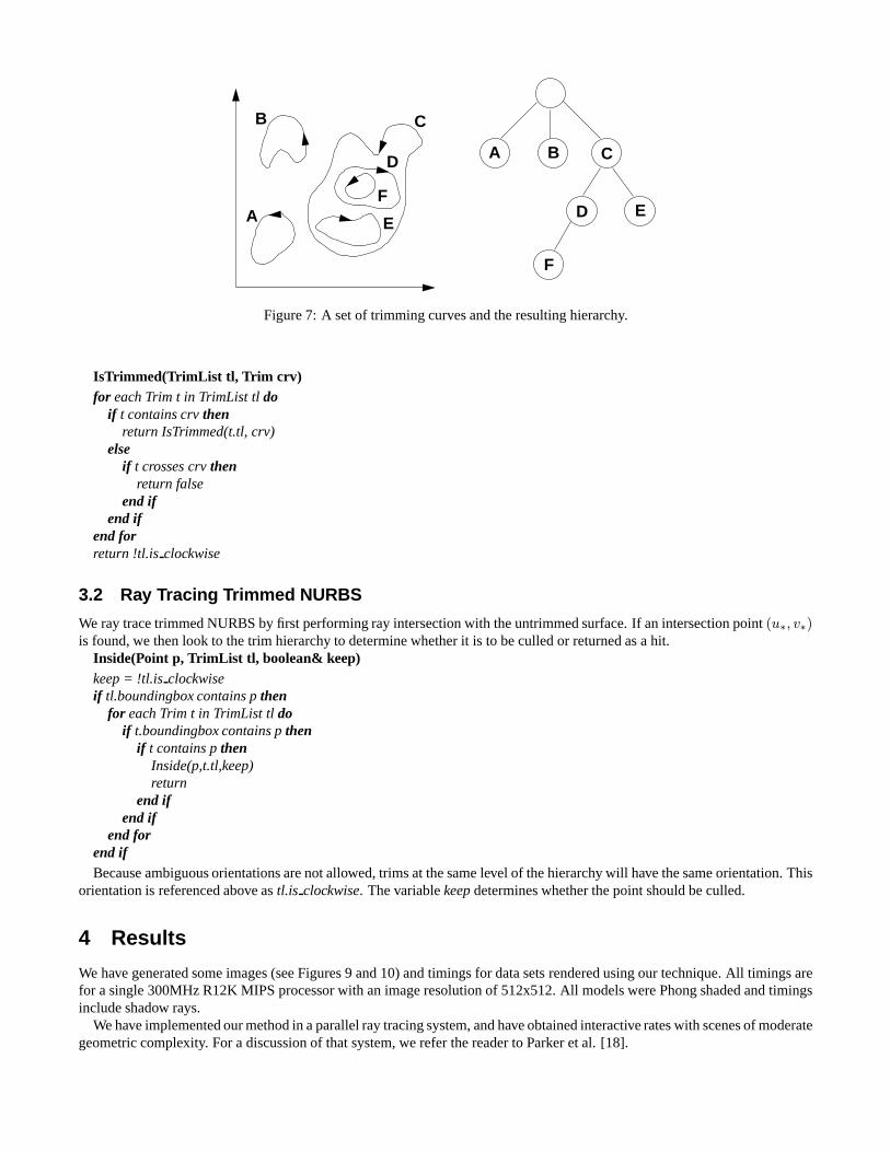
Given a set of trimming curves on a particular B-Spline surface, we can build a hierarchy based on containment (see Figure7). Since the curves are not allowed to cross, there are only three possible relationships between two curvesc1 andc2. c1 cancontainc2, be contained inc2, or share no regions in common withc2. Each node in our hierarchy is a list of trims, and eachtrim can refer to yet another list of trims which fall inside of it. Building the hierarchy proceeds as:

Insert (Trim newtrim, TrimList tl)for each Trim t in TrimList tldo

if t contains newtrimthenInsert (newtrim, t.trimlist)return

elseif newtrim contains tthen

Insert(t,newtrim.trimlist)Remove(t,tl)

end ifend if

end fortl.Add(newtrim)

Thecontainsfunction for trims needs a bit of clarification. Since trims can share edges and vertices, proper containment tests– those that test only the vertices – will not always work. Instead we perform inside/outside tests on the midpoints of each trimsegment. In comparingc1 andc2, c1 is judged to be contained inc2 if and only if the midpoint of some segment ofc1 fallsinsidec2. Since curves cannot cross, any such midpoint will do. The inside/outside test is performed with regard to someε soas to counteract round-off error.

For each trim curve, and for each trim list, we store a bounding box which we will use to speed culling in the following raytracing step.

Once the trim hierarchy is created, we perform a quick pass through the surface patches, removing those patches which arecompletely trimmed away. This is an optimization step which reduces the size of the BVH and the number of patches whichmust be examined by the intersection routines. The procedure below can be used by encoding the parametric boundary of thepatch to be tested as the trimming curvecrv.

A

B C

D

E

F

A B C

D E

F

Figure 7: A set of trimming curves and the resulting hierarchy.

IsTrimmed(TrimList tl, Trim crv)for each Trim t in TrimList tldo

if t contains crvthenreturn IsTrimmed(t.tl, crv)

elseif t crosses crvthen

return falseend if

end ifend forreturn !tl.is clockwise

3.2 Ray Tracing Trimmed NURBS

We ray trace trimmed NURBS by first performing ray intersection with the untrimmed surface. If an intersection point(u∗, v∗)is found, we then look to the trim hierarchy to determine whether it is to be culled or returned as a hit.

Inside(Point p, TrimList tl, boolean& keep)keep = !tl.is clockwiseif tl.boundingbox contains pthen

for each Trim t in TrimList tldoif t.boundingbox contains pthen

if t contains pthenInside(p,t.tl,keep)return

end ifend if

end forend ifBecause ambiguous orientations are not allowed, trims at the same level of the hierarchy will have the same orientation. This

orientation is referenced above astl.is clockwise. The variablekeepdetermines whether the point should be culled.

4 Results

We have generated some images (see Figures 9 and 10) and timings for data sets rendered using our technique. All timings arefor a single 300MHz R12K MIPS processor with an image resolution of 512x512. All models were Phong shaded and timingsinclude shadow rays.

We have implemented our method in a parallel ray tracing system, and have obtained interactive rates with scenes of moderategeometric complexity. For a discussion of that system, we refer the reader to Parker et al. [18].

Source code and other material related to the system which we have described can be found online athttp://www.acm.org/jgt/papers/MartinEtAl00.

Acknowledgments

Thanks to Michael Stark for substantial help analyzing the numerical properties of the algorithm. Thanks also to Brian Smitsfor helpful discussions, feedback, and encouragement, to Steve Parker for invaluable aid with parallelization and some of thenastier debugging, and to Amy Gooch for comments on the final draft. This work was supported in part by NSF grant 9720192(CISE New Technologies), DARPA grant F33615-96-C-5621, and the NSF Science and Technology Center for ComputerGraphics and Scientific Visualization (ASC-89-20219). All opinions, findings, conclusions or recommendations expressed inthis document are those of the authors and do not necessarily reflect the views of the sponsoring agencies.

Statistics teapot teapot-solid spoon pencilNumber of Surfaces 32 10 3 17Number of Trims 0 5 0 9Number of Rays 262144 262144 262144 262144Total Time (sec.) 14 17 4.8 10BV Intersections 12642506 10861260 3265298 3439462Light BV Intersections 6542330 5098600 902120 1714142NURBS tests 431620 642511 155118 475934Total NURBS time (sec.) 9.35 12.17 3.42 8.28Avg Time per NURBS (sec.) 2.17E-5 1.89E-5 2.20E-5 1.74E-5NURBS hits (% of tot tests) 367307 (85.1%) 458061 (71.3%) 79387 (51.2%) 226927 (47.7%)Reported hits (% of tot tests) 119597 (27.7%) 196051 (30.5%) 21753 (14.0%) 36577 (7.7%)

Statistics goblet Crank1A crank allbladeNumber of Surfaces 1 20 73 351Number of Trims 0 18 64 0Number of Rays 262144 262144 262144 262144Total Time (sec.) 7.8 78 40 61BV Intersections 3756604 23818532 14716416 47701788Light BV Intersections 1638038 6669190 3334258 17060564NURBS tests 320622 2287689 1306480 2340071Total NURBS time (sec.) 5.97 39.39 20.82 43.46Avg Time per NURBS (sec.) 1.86E-5 1.72E-5 1.59E-5 1.86E-5NURBS hits (% of tot tests) 226753(70.7%) 1488391 (65.1%) 542912 (41.6%) 1319143 (56.4%)Reported hits (% of tot tests) 100001 (31.2%) 209344 (9.2%) 103525 (7.9%) 445496 (19.0%)

Figure 8: Statistics for our technique. “Light BV intersections” are generated by casting shadow rays and are treated (and mea-sured) separately from ordinary BV intersections. “NURBS tests” gives the number of numerical NURBS surface intersectionsperformed. “Total NURBS time”and “Avg time per NURBS” give the total and mean time spent on numerical surface intersec-tions, respectively. “NURBS hits” denotes the number of numerical intersections which yielded a hit. “Reported hits” gives thenumber of successful numerical hits which were not eliminated by trimming curves or by comparison with the previous closesthit along the ray.

Figure 9: A scene containing NURBS primitives. All of the objects on the table are spline models which have been ray tracedusing the method presented in this paper.

Figure 10: Mechanical parts produced by the Alpha1 [11] modeling system (crank, Crank1A, and allblade).

References[1] Salim S. Abi-Ezzi and Srikanth Subramaniam. Fast dynamic tessellation of trimmed NURBS surfaces. InEurographics ’94, 1994.

[2] Richard H. Bartels, John C. Beatty, and Brian A. Barsky.An introduction to splines for use in computer graphics and geometric modeling. Morgan Kauffman Publishers, Inc.,Los Altos, CA, 1987.

[3] W. Barth and W. St¨urzlinger. Efficient ray tracing for B´ezier and B-spline surfaces.Computers and Graphics, 17(4), 1993.

[4] W. Boehm. Inserting new knots into B-spline curves.Computer-Aided Design, 12:199–201, July 1980.

[5] Swen Campagna, Philipp Slusallek, and Hans-Peter Seidel. Ray tracing of spline surfaces: B´ezier clipping, Chebyshev boxing, and bounding volume hierarchy – a criticalcomparison with new results. Technical report, University of Erlangen, IMMD IX, Computer Graphics Group, Am Weichselgarten 9, D-91058 Erlangen, Germany, October1996.

[6] E. Cohen, T. Lyche, and R. Riesenfeld. Discrete B-splines and subdivision techniques in computer-aided geometric design and computer graphics.Comput. Gr. Image Process.,14:87–111, October 1980.

[7] Gerald E. Farin.Curves and surfaces for computer aided geometric design: a practical guide, 4th ed.Academic Press, Inc., San Diego, CA, 1996.

[8] Alain Fournier and John Buchanan. Chebyshev polynomials for boxing and intersections of parametric curves and surfaces. InEurographics ’94, 1994.

[9] Andrew Glassner, ed. An introduction to ray tracing. 1989.

[10] Josef Hoschek and Dieter Lasser.Fundamentals of computer aided geometric design. A.K. Peters, Wellesley, MA, 1993.

[11] Integrated Graphics Modeling Design and Manufacturing Research Group.Alpha1 geometric modeling system, user’s manual. Department of Computer Science, Universityof Utah.

[12] James T. Kajiya. Ray tracing parametric patches.Computer Graphics (SIGGRAPH ’82 Proceedings), 16(3):245–254, July 1982.

[13] Subodh Kumar, Dinesh Manocha, and Anselmo Lastra. Interactive display of large NURBS models.IEEE Transactions on Visualization and Computer Graphics, 2(4),December 1996.

[14] Daniel Lischinski and Jakob Gonczarowski. Improved techniques for ray tracing parametric surfaces.The Visual Computer, 6(3):134–152, June 1990. ISSN 0178-2789.

[15] William L. Luken and Fuhua (Frank) Cheng. Comparison of surface and derivative evaluation methods for the rendering of NURB surfaces.ACM Transactions on Graphics,15(2):153–178, April 1996. ISSN 0730-0301.

[16] T. Lyche, E. Cohen, and K. Morken. Knot line refinement algorithms for tensor product B-spline surfaces.Computer Aided Geometric Design, 2(1-3):133–139, 1985.

[17] Tomoyuki Nishita, Thomas W. Sederberg, and Masanori Kakimoto. Ray tracing trimmed rational surface patches. InSIGGRAPH ’90, 1990.

[18] Steven Parker, William Martin, Peter-Pike J. Sloan, Peter Shirley, Brian Smits, and Charles Hansen. Interactive ray tracing.1999 ACM Symposium on Interactive 3D Graphics,pages 119–126, April 1999. ISBN 1-58113-082-1.

[19] John W. Peterson. Tessellation of NURBS surfaces. In Paul Heckbert, editor,Graphics Gems IV, pages 286–320. Academic Press, Boston, 1994.

[20] Les A. Piegl and W. Tiller.The NURBS Book. Springer Verlag, New York, NY, 1997.

[21] William H. Press, Saul A. Teukolsky, William T. Vetterling, and Brian P. Flannery. Numerical recipes in C: The art of scientific computing (2nd ed.). 1992. ISBN 0-521-43108-5.Held in Cambridge.

[22] Alyn Rockwood, Kurt Heaton, and Tom Davis. Real-time rendering of trimmed surfaces. InSIGGRAPH ’89, 1989.

[23] Jon Rokne. The area of a simple polygon. In James R. Arvo, editor,Graphics Gems II. Academic Press, 1991.

[24] Brian Smits. Efficiency issues for ray tracing.Journal of Graphics Tools, 3(2):1–14, 1998. ISSN 1086-7651.

[25] Michael A.J. Sweeney and Richard H. Bartels. Ray tracing free-form B-spline surfaces.IEEE Computer Graphics & Applications, 6(2), February 1986.

[26] Thomas V. Thompson II and Elaine Cohen. Direct haptic rendering of complex NURBS models. InProceedings of Symposium on Haptic Interfaces, 1999.

[27] Daniel L. Toth. On ray tracing parametric surfaces.Computer Graphics (Proceedings of SIGGRAPH 85), 19(3):171–179, July 1985. Held in San Francisco, California.

[28] Chang-Gui Yang. On speeding up ray tracing of B-spline surfaces.Computer Aided Design, 19(3), April 1987.