NBER WORKING PAPER SERIES

TECHNOLOGY DIFFUSION AND PRODUCTIVITY GROWTH IN HEALTH CARE

Jonathan SkinnerDouglas Staiger

Working Paper 14865http://www.nber.org/papers/w14865

NATIONAL BUREAU OF ECONOMIC RESEARCH1050 Massachusetts Avenue

Cambridge, MA 02138April 2009

We are grateful to seminar participants at Brown, Chicago, CUNY/Columbia, Harvard, MIT, MichiganState, UC Berkeley, The University of Illinois (Chicago and Champaign-Urbana), Rutgers, Case-Western,and to Mary Burke, David Card, Amitabh Chandra, James Feyrer, Elliott Fisher, Sherry Glied, CarolineHoxby, Peter Klenow, Justin McCrary, David Weil, Milton Weinstein, and Jack Wennberg for helpfulcomments. Weiping Zhou and Daniel Gottlieb provided superb data analysis. We are indebted to theNational Institute on Aging (PO1-AG19783) and the Robert Wood Johnson Foundation for financialsupport. The views expressed herein are those of the author(s) and do not necessarily reflect the viewsof the National Bureau of Economic Research.

NBER working papers are circulated for discussion and comment purposes. They have not been peer-reviewed or been subject to the review by the NBER Board of Directors that accompanies officialNBER publications.

© 2009 by Jonathan Skinner and Douglas Staiger. All rights reserved. Short sections of text, not toexceed two paragraphs, may be quoted without explicit permission provided that full credit, including© notice, is given to the source.

Technology Diffusion and Productivity Growth in Health CareJonathan Skinner and Douglas StaigerNBER Working Paper No. 14865April 2009JEL No. H51,I1,O33

ABSTRACT

Inefficiency in the U.S. health care system has often been characterized as “flat of the curve” spendingproviding little or no incremental value. In this paper, we draw on macroeconomic models of diffusionand productivity to better explain the empirical patterns of outcome improvements in heart attacks(acute myocardial infarction). In these models, small differences in the propensity to adopt technologycan lead to wide and persistent productivity differences across countries -- or in our case, hospitals.Theoretical implications are tested using U.S. Medicare data on survival and factor inputs for 2.8 millionheart attack patients during 1986-2004. We find that the speed of diffusion for highly efficient andoften low-cost innovations such as beta blockers, aspirin, and primary reperfusion explain a large fractionof persistent variations in productivity, and swamp the impact of traditional factor inputs. Holdingtechnology constant, the marginal gains from spending on heart attack treatments appear positive butquite modest. Hospitals which during the period 1994/95 to 2003/04 raised their rate of technologydiffusion (the “tigers”) experienced outcome gains four times the gains in hospitals with diminishedrates of diffusion (the “tortoises”). Survival rates in low-diffusion hospitals lag by as much as a decadebehind high-diffusion hospitals, raising the question of why some hospitals (and the physicians whowork there) adopt so slowly.

Jonathan SkinnerDepartment of Economics6106 Rockefeller HallDartmouth CollegeHanover, NH 03755and NBERjonathan.skinner@dartmouth.edu

Douglas StaigerDepartment of Economics6106 Rockefeller HallDartmouth CollegeHanover, NH 03755and NBERdouglas.staiger@dartmouth.edu

1

1. Introduction

There are pervasive regional differences in per capita U.S. Medicare expenditures,

ranging from $5,877 in Salem, OR to $16,351 in Miami.1 Yet there is little or no evidence that

the higher spending in high cost regions lead to better outcomes, with estimates of inefficiency

range from 20 to 30 percent of overall health care expenditures (Fisher et al., 2003; Skinner, et

al., 2005). These estimates have been interpreted as “flat of the curve” health care spending, or

variations along a common production function with a very low or zero marginal value of health

care spending.2

But this “flat of the curve” explanation is problematic for many observed patterns. First,

Baicker and Chandra (2004) have documented that state-level quality measures are negatively

associated with per capita Medicare expenditures. Why should spending more be associated

with providing worse quality care? Second, given results from Cutler, et al. (1998), Berndt et al.

(2002), and others that over time, survival and functioning has improved because of often

expensive new medical technology, it would be surprising if 20 to 30 percent of health care

spending (or between 3 and 4.5 percent of GDP) should provide no benefit whatsoever.

In this paper, we draw on macroeconomic models of productivity to provide a better

explanation for these empirical puzzles. That differential rates of technology adoption can

explain long-term variations in per capita GDP across countries is by now well understood.

Crespi, et al. (2008) find as much as 50 percent of total factor productivity growth arises simply

from the flow of knowledge across firms. Parente and Prescott (1994, 2002) showed that

surprisingly small differences in the rates of technological adoption could imply large disparities

1 Estimates are for 2006 (www.dartmouthatlas.org). 2 See e.g., Fuchs (2004) and Enthoven (1978).

2

in country levels of income, while Eaton and Kortum (1999) estimated that countries realized

just two-thirds of the potential productivity gains because of the slow diffusion and adoption of

ideas across borders (see Hall, 2004).

There is a parallel literature in health care documenting similar lags in adoption, and with

similar adverse effects on overall productivity. For example, despite powerful evidence from a

1601 experiment demonstrating the effectiveness of lemon juice in preventing scurvy, the British

Navy did not require foods containing vitamin C until 1794 (Berwick, 2003).3 Yet during the

18th century, more men in the British Navy died of scurvy than were lost to battle casualties (Lee,

2004). More recently, beta blockers, drugs costing pennies per dose, were shown during the

early 1980s to reduce mortality by as much as 25 percent following a heart attack (Yusuf, et al.,

1985). By 2000/2001, the median state-level use of beta Blockers among appropriate patients

was still only 68 percent (Jencks, et al., 2003).

We develop a model in which output (survival) depends on factor inputs and the speed of

technology diffusion. The hospital is assumed to maximize the present value of lives saved

minus resource and learning costs. This in turn yields testable implications for the nature and

extent of lags in total factor productivity among hospitals. We apply this model to the hospital-

level treatment of patients diagnosed with an acute myocardial infarction (AMI, or a heart attack)

using data on hospital-specific technology diffusion during 1994/95 for three inputs: aspirin, beta

blockers, and reperfusion within 12 hours of the heart attack. (Reperfusion consists either of

thrombolytic “clot-busting” drugs, or surgical angioplasty.) These treatments are: (a) proven to

be effective in saving lives, (b) not so expensive as to cause financial barriers to diffusion, and

3 In his 1601 voyage to India, Captain James Lancaster fed sailors in one of his ships 3 teaspoons of lemon juice every day, while in the other three ships, no lemon juice was provided. By the midpoint of the journey, 110 of the 278 sailors in the control group had died of scurvy (40 percent), while none of the sailors in the treatment group had been affected (Berwick, 2003).

3

(c) administered based on the decision of the physician, not by the supine heart attack patient.

As well, we examine the diffusion of a much newer technology first introduced in 2003, drug-

eluting stents, to identify changes over time in the speed with which new innovations diffuse in

the hospital.

The model is tested using a sample of 2.8 million heart attack patients drawn from the

fee-for-service Medicare population during 1986-2004. Hospitals are initially categorized into

quintiles based on the diffusion of effective treatments in 1994/95. Like Comin and Hobijn

(2004, 2008) who study country-level data, we find that hospitals with rapid diffusion in one

highly effective technology are more likely to adopt other technologies. More importantly, we

find that the 1994/95 quintiles of technology diffusion explain large variations across hospitals in

risk-adjusted survival, and that these productivity effects swamp the influence of differences in

factor inputs -- a result also found in the macroeconomics literature (e.g., Hall and Jones, 1999).

And like Eaton and Kortum’s (1999) study of aggregate productivity, we find substantial

differences in the extent to which some hospitals lag behind, with an average gap of 3.3

percentage points in one-year survival between rapid-diffusing and slow-diffusing hospitals,

nearly one-third of the overall improvement in outcomes during 1986-2004. Finally, we find that

the “Asian tiger” hospitals which between 1994/95 and 2003/04 demonstrated dramatic

improvements in diffusion rates also experienced above-average survival growth, and four times

the growth in the “tortoise” hospitals that experienced a decline in diffusion rates.

These results can potentially reconcile the two views of the U.S. health care system.

Technological progress has led to dramatic improvements in survival for heart attack patients (as

in Cutler, 2004), but these improvements are largely associated with the adoption of relatively

inexpensive but effective treatments, rather than more factor inputs per se. Holding technology

diffusion constant, however, we find modest improvements in outcomes associated with

4

spending more, with a preferred estimate of (at best) about $95,000 per life year during this

period. At least for heart attacks, our results are inconsistent with the prevailing “flat of the

curve” view of health care spending in the U.S.

The real puzzle is why many physicians and hospitals remain so far behind the

production possibility frontier, contributing to a remarkable degree of productive inefficiency in

health care. As we discuss below, our model suggests that some hospitals must either face very

high barriers to the diffusion of effective health technologies, or must substantially undervalue

the survival benefits of these technologies. In the conclusion, we speculate about why this might

be the case for hospitals, and for technology diffusion more generally.

2. The Model

We focus on the “production” of survival following acute myocardial infarction (AMI).

There are compelling reasons to focus on heart attacks. Nearly every AMI patient who survives

the initial attack is admitted to a hospital, and ambulance drivers generally take the patient to the

nearest hospital. The outcome, survival, is accurately measured and there is broad clinical

agreement that survival is the most important endpoint, particularly in the elderly population.

The measurement of inputs is also accurate, as is risk adjustment including the type of heart

attack. Finally, many of the studies focusing on the value of medical technology have used AMI

as an example (Cutler, et al., 1998; Cutler, 2004).

The Hospital Production Function. We develop a simple model of hospital productivity

that distinguishes between inputs that require substantial contributions of capital and labor (e.g.,

hospital bed-day or surgical procedures) and technology innovations where barriers are unlikely

to arise solely from financial constraints. Suppose that medical care per patient (e.g. quantity of

medical services) at hospital i in year t (Xit) is produced with constant returns technology:

5

(1) ξξ −= 1ititit khlX

where lit and kit represent labor and capital inputs per patient at hospital i in year t, and h is a

constant measure of productivity in producing X. Letting r denote the cost of capital and w the

wage rate, the efficient marginal expenditure per X (the implicit price) is

ξξ

ξξ

−−

⎟⎟⎠

⎞⎜⎜⎝

⎛−⎟⎟

⎠

⎞⎜⎜⎝

⎛=

11

1itit

itrwhP . Because our data measures Xit more accurately than capital and labor

inputs, we focus on the composite factor input rather than on capital and labor separately.4

While it seems reasonable to assume constant returns for producing medical care services

(doubling staff and beds at a hospital can produce twice the number of admissions), we assume

that medical care per patient has declining returns in terms of patient survival (or quality adjusted

life years). We assume initially a simple production function that specifies a linear relationship

between survival per patient (yit,), the log of composite medical care inputs xit = ln(Xit,), and the

level of technology at hospital i at time t, ait

(2) itxitaity β+=

We adopt this special case to simplify the balanced-growth path of technological innovation, but

in the empirical section allow for the more general translog production model (Christiansen,

Jorgenson, and Lau, 1973), which allows for the marginal productivity of Xit to depend on

technology.

The Diffusion of Technology. Technology is modeled as the sum of many separate

innovations, and for simplicity we assume a model of certainty in which one new innovation

becomes available each year. Letting j index the year the innovation first appeared yields:

4 In theory one could measure Part A hospital days and Part B physician resource-value units (RVUs), but the Part B data is available for just a 5 percent sample in earlier years, nor is hospital days always a good measure of health care intensity. See also Jacobs, Smith, and Street (2006) for an excellent discussion of measuring productivity in X.

6

(3) ∑=

=t

jjitjit ma

1

α

In Equation (3), mijt is the fraction of appropriate patients at hospital i receiving treatment j (or

the proportion of physicians who have adopted innovation j) by time t, while jα is the return to

adopting innovation j. The adoption rate in turn is written

(4) )1( 11 −− −+= jititjitjit mmm π

In other words, this year’s usage rate m is equal to last year’s rate plus the institutional- and

time-specific “core” diffusion rate πit times the gap between best-practice (100 percent use) and

last year’s usage. We assume that each hospital chooses its adoption hazard across all new

innovations at each point in time; we show below that this adoption rate is constant over time in

steady-state.

The frontier technology available at time t, at*, is the technology that could be achieved if

a hospital had fully adopted all innovations available,

(5) ∑=

=t

jjta

1

* α

Thus, combining equations (3)-(5), the technology level at a given point in time can be written

(6) )( *11 ittititit aaaa −+= ++ π

Equation (6) is the Nelson-Phelps (1966) partial adjustment model for productivity, where the

diffusion rate (πit) determines the rate of partial adjustment in productivity toward the frontier

that is achieved each year.

Finally, we assume that there is a cost per patient of encouraging rapid adoption and

diffusion, Ci(πit), with C’ > 0 and C” > 0. The costs may include the obvious expenses of (e.g.)

computerized information systems that prompt physicians when beta blockers or aspirin have not

been administered, quality improvement initiatives, or higher wages and research time to help

7

recruit smarter or more technically skilled physicians (Bero, et al., 1998; Bradley, et al., 2001).

These costs (and marginal costs) are likely to differ substantially across hospitals, and will likely

reflect other factors that affect the speed of diffusion (e.g., Rogers, 2003). This approach

parallels other models in which physicians face different search costs and may hold different

views about the value of new technology (see Phelps, 2000).

The Hospital Objective Function. There is considerable debate about the objective

function of hospitals (e.g., Horwitz and Nichols, 2007); to avoid having to choose a specific

model, we instead adopt a general objective function depending positively on survival and

negatively on costs:

(7) [ ] tititiititiititi

ti rKCXPxaV −

∞

=

++−−+Ψ=∑ )1()()(0

πϕβ

where r is the discount rate, Ψi is the implicit social (dollar) value of improved health (assumed

for simplicity to be constant over time), while Kit represents either fixed costs or subsidization

from endowments or non-Medicare patient revenue. The provider-specific parameter φi reflects

variation in the degree to which hospitals trade off the social cost of increasing Xit with the

potential private benefits of doing more; for example when cardiac surgery generates profits, φi

could be lower. Consider the special case where Ψi is equal to the social value of survival, and φi

is one; for this case hospitals maximize social surplus. As we show in the Appendix, other

models of hospital behavior reflecting the tension between financial profits and social welfare

imply values of Ψi and φi below those corresponding to a social planner.

Solving the Dynamic Model. The maximization is subject to the equations denoting the

evolution of technology over time, and is expressed as a discrete-time Lagrangian;

(8) )]([ *1

01 ittitit

tititi aaaaV −−−−=ℑ +

∞

=+∑ πλ

8

This model can also be written in continuous time as a current-value Hamiltonian, but we

maintain a discrete time structure to help specify the empirical model. Under constant

productivity growth, where αt = α and at+1* = at* + α, the first-order conditions (shown in

Appendix Equations A.4a through A.4d) yield a dynamic steady-state path with an equilibrium

(and stable) diffusion rate πi that is constant over time.

From the first-order conditions, optimal factor inputs are given by

(9) iitiit PX ϕβ /Ψ= .

Not surprisingly, factor inputs are greater when there is a higher implicit value by the hospital on

saving a life-year Ψi, when the price of producing a factor input Pit is lower, and when financially

motivated hospitals are reimbursed generously for care (φi is small). Optimal factor inputs are

independent of the level of technology because the production function (Equation 2) assumes

that the marginal product of factor inputs (β) does not depend on technology. In a more general

specification that allowed for interactions between technology and factor inputs, optimal factor

inputs would increase (decrease) if new technology increased (decreased) the marginal product

of factor inputs.

For a constant growth rate α, it is straightforward to show that productivity in the steady

state is given by:

(10) ⎟⎟⎠

⎞⎜⎜⎝

⎛ −−=

i

itit aa

ππ

α1*

Equation (10) states that the steady-state distance that a hospital lags behind the productivity

frontier is a constant nonlinear function of the diffusion rate, in which small differences in

diffusion can lead to very large differences in productivity (Parente and Prescott, 1994). Note

that the term ii ππ /)1( − can be interpreted as the number of years a hospital lags behind the

frontier (since α is annual productivity growth). Thus, a hospital with a 20% diffusion rate lags 4

9

years behind, and a hospital with a 5% diffusion rate lags 19 years behind. Equation 10 also

implies that there is no convergence; productivity at all hospitals grows at the same rate as the

frontier – α. This property has been noted in other papers as well (Eaton and Kortum, 1999) and

is a consequence of the Nelson-Phelps (1966) partial adjustment model implied by Equation 6.

Finally, the optimal diffusion rate is chosen to set its marginal cost equal to its marginal

benefit:

(11) ( )π

π+−Ψ

=r

aaC ttt

*

)('

The numerator of the right-hand side of Equation 11 measures the immediate benefit, in dollar

terms, of moving to the frontier today, while the denominator converts this to the present value,

as the value of today’s innovation decays in the future. Notice that the value of the incremental

innovation decays both by the interest rate r, but also by the diffusion rate π; the value of

adopting today is attenuated by the likelihood of adopting anyway sometime in the future, under

than the status-quo π. Note that we can use Equation 11 to back out the implicit marginal cost of

raising the underlying diffusion rate. We consider below plausible sets of parameters that satisfy

this first-order condition.

3. Empirical Specification

We now translate the theoretical model to a stochastic specification with measurement

error. We rewrite Equation (2) but add an error term uit without yet making any claims for its

statistical properties:

(12) itititit uxay ++= β

Using the steady-state assumption from Equation (11), Equation (12) is rewritten

(13) ititi

itit uxay ++⎥

⎦

⎤⎢⎣

⎡ −−= β

ππ

α1*

10

This suggests a very simple estimation model, regressing survival (yit) on log inputs (xit), a linear

trend (or year fixed effects) to reflect growth over time in the frontier at*, and a variable

reflecting the hospital-specific rate of diffusion πi. However, several challenges remain: xit and

yit must be constructed from individual-level data; πi is not directly observable and must be

estimated, and may change over time; the linear estimation equation may be too restrictive; and u

could be correlated with x. We consider each of these issues in turn.

Creating hospital-level survival and input measures. We create hospital-level measures

of survival and factor inputs from the individual data in the Medicare claims data. Let one-year

mortality following a heart attack be expressed as:

(14) lit

H

iitlitlit eZS ++Γ= ∑

=1

γ

The dependent variable, Slit is a one-zero variable reflecting whether the individual l who had an

AMI in year t (and was admitted to hospital i) survived for at least one year, with Zlit a matrix of

individual risk-adjusters, Γ a vector of coefficient, γit a vector of hospital-year specific intercepts,

and elit the error term. Similar equations are also estimated for two measures of total factor

inputs in the year following the heart attack: Hospital expenditures (in constant 2004 dollars),

and the sum of diagnostic-related group (or DRG) weights across all hospital admissions, which

reflect the Centers for Medicare and Medicaid Services (CMS) assessment of resources

necessary to provide specific and detailed procedures. The hospital-year intercepts from

Equation 14 (γit) are used in our subsequent estimation as risk-adjusted measures of survival and

factor inputs.

Estimating each hospital’s rate of diffusion. We use data on the diffusion of various

innovations at a point in time to estimate the underlying diffusion rate at each hospital. In steady-

state with a constant hospital-specific πi, equation (4) implies that the cumulative adoption of

11

each innovation can be expressed as jtijitm −−−= )1(1 π , where mjit is as before the (fractional)

use of the jth innovation at hospital i and time t. In other words, the current rate of use of an

innovation depends simply on the number of years it has been available (t-j) and the “core” speed

of adoption at the hospital (πi). Taking a first order approximation that (t-j)πi ≈ jti

−−− )1(1 π and

adding a stochastic term ( jitv ) to allow for random fluctuations over time allows us to express

mjit as

(15) jitijit vjtm +−= π)( .

Equation 15 describes a factor model, in which the dependent variable is the adoption

rate of a given innovation by a given year, the common factor (πi) captures the intensity of search

for new innovations at hospital i, and the factor loading (t-j) reflects the length of time the

innovation has been available. Therefore, we fit a factor model to hospital-level data on the

adoption rate of various innovations, and use the prediction of the common factor as a proxy for

each hospital’s underlying diffusion rate.

There are two approaches to estimating the influence of this diffusion parameter on

survival. One is to simply enter the common factor (which is proportional to πi, but normalized

to have mean zero and standard deviation one) linearly on the right-hand side of Equation (13).

But Equation (13) implies a nonlinear influence of π on survival, and so we also create patient-

weighted hospital-level quintiles of the common diffusion factor. Finally, in some specifications

of equation (13) we include hospital fixed effects to proxy for each hospital’s diffusion

parameter. Hospital fixed effects do not provide a direct estimate of how diffusion is associated

with patient survival, but they avoid concerns about poorly measured estimates of πi, resulting in

estimates of β that are less subject to omitted variable bias due to unmeasured differences in

diffusion.

12

Relaxing the assumption of a steady-state model. If hospitals are not in steady-state (e.g.,

because of changing costs of diffusion) then πit will not be constant over time, and the equation

for current survival becomes more complex. Using a first order approximation (valid for small

πit), equation (13) becomes :

(16) itit

t

kikit uxky ++=∑

=

βαπ1

where the summation captures the impact of the diffusion in each time period k on all k

innovations that were available at that time. One approach to testing the model is to study

survival rates of hospitals experiencing large changes in measured diffusion; from (16) one can

see that changing rates of diffusion will shift health outcomes upward (the productivity “tigers”)

or downward (the “tortoises”) to new steady-state output levels.

A semi-parametric approach to estimating the model. In some specifications, we estimate

a flexible translog production function (Christiansen, Jorgenson, and Lau, 1973) to allow for

diminishing returns to xit, and interaction between diffusion and the productivity of xit:

(17) itititititititit uxaxaxay +++++= 23

221 νννβ

We estimate this model in a slightly more general formulation, by stratifying across quintiles of

diffusion and allowing coefficients on xit and xit2 to vary across quintiles.

The error term could be correlated with factor inputs. Estimates of the return to factor

inputs (β) in Equation (13) may be biased by correlation between factor inputs (xit) and the error

term. There are two reasons to suspect such a correlation.

First, if there are interactions between technology and the return to factor inputs (as

would be the case in the translog specification), then the optimal factor inputs will depend on the

level of technology at each hospital. To the extent that our proxy for technology diffusion at each

hospital is imperfect, the error term in Equation (13) will reflect some remaining technology

13

differences. This will bias the coefficient on factor inputs downwards (upwards) if higher levels

of technology are associated with lower (higher) optimal use of factor inputs. To investigate the

importance and direction of the bias arising from omitted technology differences, we present two

types of evidence. First, we estimate Equation (13) with more and less detailed controls for

technology diffusion, ranging from no controls to hospital fixed effects.5 Second, we estimate the

more general translog specification in Equation (17) to investigate whether the return to factor

inputs varies with technological diffusion.

A second reason to suspect a correlation between factor inputs and the error term arises

from our construction of yit and xit from individual data – small numbers of people in each

hospital-year observation could create a spurious positive correlation between yit and xit, given

that (as we find in the data) people who live longer also tend to account for more spending. To

address this issue, we also present estimates that replace xit with lagged measures of factor inputs

xit-1, thus sampling the independent variable from the year t group of patients and the dependent

variables from the year t-1 group. Instead, independent sampling error in xit-1 will bias the

coefficient toward zero.

One approach to the endogeneity of factor inputs, which we do not take, is to estimate an

instrumental variables model that seeks to express xit in terms of “fundamentals.” Note that we

have already derived the first-order conditions for X in Equation (9); in log terms one can write:

(9’) )ln()ln(ln)ln( iitiit Px ϕβ −−+Ψ=

It is certainly possible to think of factors that might be associated with each parameter, for

example for-profit or government status of the hospital (leading to a lower or higher iϕ ), or

higher state-level income (positively associated with Ψ). But all of the variables we considered

5 Even with hospital fixed effects there may be bias because of changing technology diffusion over time.

14

are inappropriate instruments because they are likely to affect survival beyond their impact on xit.

Rather than use questionable instruments, we eschew the IV approach and interpret the estimate

of β with caution.

The cost-effectiveness ratio. To provide a basis for comparison with other studies, we

also calculated the “cost-effectiveness” (CE) ratio, or the cost per life-year gained, defined as

(18) ⎥⎦

⎤⎢⎣

⎡=

dydL

dXdy

dXdCCE

where X measures DRGs (and dC/dX is the cost per DRG) y is the probability of surviving one

year, dy/dX is derived from the regression estimate, and dL/dy, the change in life expectancy

conditional on surviving an extra year, is set to 5.25 based on estimates in Cutler et al. (1998).6

There is some debate over the appropriate hurdle for whether a treatment is cost-

effective. Generally, values below $100,000 per life year pass muster, although some clinical

willingness-to-pay estimates are well below $50,000 (King et al., 2005). Conversely, economists

often favor much larger estimates, of up to $250,000 per life year for older people (Hirth, et al.,

2000, Murphy and Topel, 2006).

4. The Diffusion of Efficient Treatments for Acute Myocardial Infarction

Information on technology diffusion was measured in the Cooperative Cardiovascular

Program (CCP) dataset, which involved chart reviews for over 160,000 AMI patients over age 65

during 1994/95, matched to the admitting hospital. We chose three measures of low-cost but

effective innovations. The first, aspirin, reduces platelet aggregation and helps to limit clotting,

thereby improving blood flow to the oxygen-starved tissue, and by 1988 it was included in

6 The average inpatient cost of one year of inpatient treatment following AMI was equal to equal to $26,063 in 2004. These estimates ignore outpatient and physician costs, which are likely to add at least 15% to costs (and hence 15% to the CE ratio). The equation simplifies when we use expenditures rather than DRGs as inputs.

15

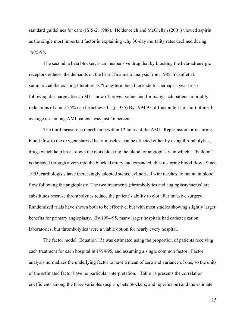
standard guidelines for care (ISIS-2, 1988). Heidenreich and McClellan (2001) viewed aspirin

as the single most important factor in explaining why 30-day mortality rates declined during

1975-95.

The second, a beta blocker, is an inexpensive drug that by blocking the beta-adrenergic

receptors reduces the demands on the heart. In a meta-analysis from 1985, Yusuf et al.

summarized the existing literature as “Long-term beta blockade for perhaps a year or so

following discharge after an MI is now of proven value, and for many such patients mortality

reductions of about 25% can be achieved.” (p. 335) By 1994/95, diffusion fell far short of ideal:

average use among AMI patients was just 46 percent.

The third measure is reperfusion within 12 hours of the AMI. Reperfusion, or restoring

blood flow to the oxygen-starved heart muscles, can be effected either by using thrombolytics,

drugs which help break down the clots blocking the blood, or angioplasty, in which a “balloon”

is threaded through a vein into the blocked artery and expanded, thus restoring blood flow. Since

1995, cardiologists have increasingly adopted stents, cylindrical wire meshes, to maintain blood

flow following the angioplasty. The two treatments (thrombolytics and angioplasty/stents) are

substitutes because thrombolytics reduce the patient’s ability to clot after invasive surgery.

Randomized trials have shown both to be effective, but with most studies showing slightly larger

benefits for primary angioplasty. By 1994/95, many larger hospitals had catheterization

laboratories, but thrombolytics were a viable option for nearly every hospital.

The factor model (Equation 15) was estimated using the proportion of patients receiving

each treatment for each hospital in 1994/95, and assuming a single common factor. Factor

analysis normalizes the underlying factor to have a mean of zero and variance of one, so the units

of the estimated factor have no particular interpretation. Table 1a presents the correlation

coefficients among the three variables (aspirin, beta blockers, and reperfusion) and the estimate

16

of the common factor. The correlation of each input with the common factor ranges from 0.87

for beta blockers to 0.30 for reperfusion, demonstrating that hospitals that adopt one innovation

early are also more likely to adopt other innovations. Note that the correlation between beta

blockers and reperfusion is only 0.03, reflecting in part the specialization of some hospitals into

surgical treatments for AMI (Chandra and Staiger, 2007).

In Table 1b, we show that the quintiles based on this common factor show clear

differences in the use of beta blockers (from 65 percent in the highest adopting Quintile 5 to 31

percent in the lowest Quintile 1) and aspirin (90 percent to 65 percent), with more modest

differences in reperfusion (21 percent to 15 percent).7 One could interpret these patterns as

reflecting demand; patients in high quintile regions ask for and get beta blockers, for example.

But this seems unlikely; elderly heart attack patients are unlikely to be requesting specific

treatments, with few knowing the value of beta blockers or aspirin. More to the point,

hospitalized patients should not have to ask their physicians for these treatments given their clear

benefits.

Table 1b also demonstrates that hospitals in the quintiles with quicker adoption also have

higher patient volume, are more likely to be major teaching hospitals, and are located in states

with slightly higher average income (which proxies for a higher social value per life year).

These hospitals are likely to experience both a lower marginal cost of diffusion and place a

higher value on more rapid diffusion.

The 1993/94 diffusion measures provide two independent predictions on steady-state

differences in productivity across quintiles of hospitals. The first arises from the implications of

7 These averages are for all patients and not for “ideal” patients; since it is often difficult in practice to define ideal or appropriate patients. While a high fraction of patients should receive β blockers and aspirin, the optimal rate for revascularization is substantially lower.

17

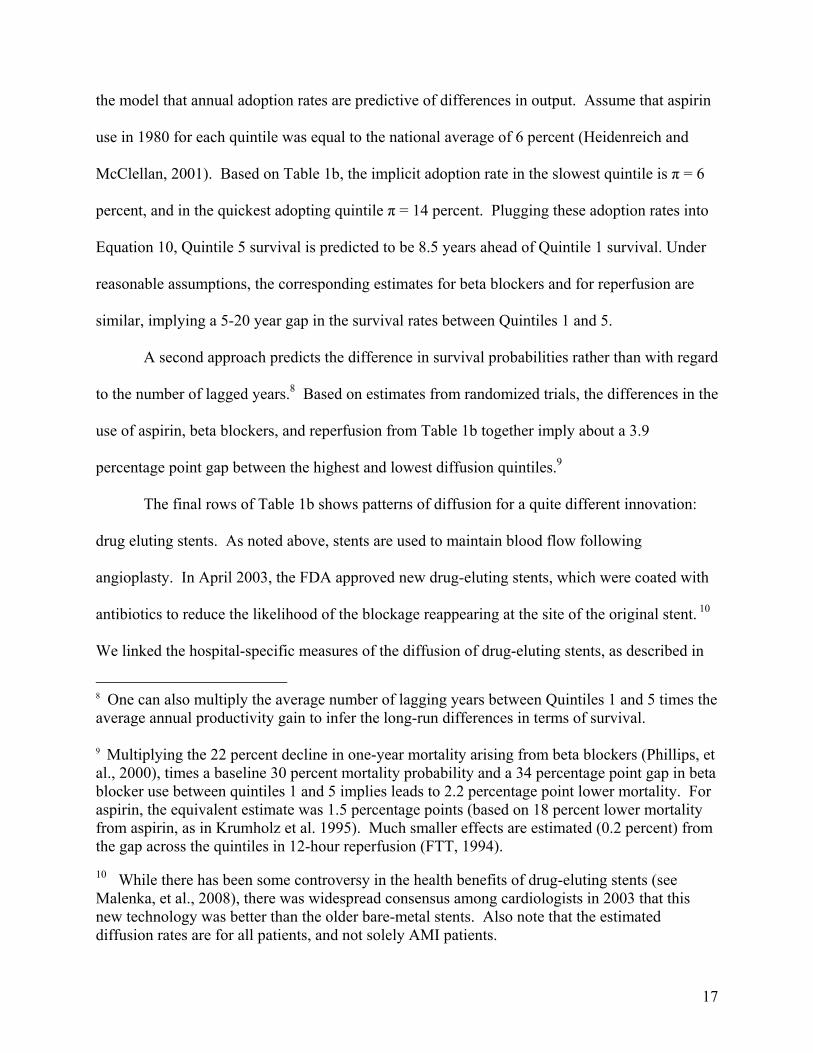
the model that annual adoption rates are predictive of differences in output. Assume that aspirin

use in 1980 for each quintile was equal to the national average of 6 percent (Heidenreich and

McClellan, 2001). Based on Table 1b, the implicit adoption rate in the slowest quintile is π = 6

percent, and in the quickest adopting quintile π = 14 percent. Plugging these adoption rates into

Equation 10, Quintile 5 survival is predicted to be 8.5 years ahead of Quintile 1 survival. Under

reasonable assumptions, the corresponding estimates for beta blockers and for reperfusion are

similar, implying a 5-20 year gap in the survival rates between Quintiles 1 and 5.

A second approach predicts the difference in survival probabilities rather than with regard

to the number of lagged years.8 Based on estimates from randomized trials, the differences in the

use of aspirin, beta blockers, and reperfusion from Table 1b together imply about a 3.9

percentage point gap between the highest and lowest diffusion quintiles.9

The final rows of Table 1b shows patterns of diffusion for a quite different innovation:

drug eluting stents. As noted above, stents are used to maintain blood flow following

angioplasty. In April 2003, the FDA approved new drug-eluting stents, which were coated with

antibiotics to reduce the likelihood of the blockage reappearing at the site of the original stent. 10

We linked the hospital-specific measures of the diffusion of drug-eluting stents, as described in

8 One can also multiply the average number of lagging years between Quintiles 1 and 5 times the average annual productivity gain to infer the long-run differences in terms of survival. 9 Multiplying the 22 percent decline in one-year mortality arising from beta blockers (Phillips, et al., 2000), times a baseline 30 percent mortality probability and a 34 percentage point gap in beta blocker use between quintiles 1 and 5 implies leads to 2.2 percentage point lower mortality. For aspirin, the equivalent estimate was 1.5 percentage points (based on 18 percent lower mortality from aspirin, as in Krumholz et al. 1995). Much smaller effects are estimated (0.2 percent) from the gap across the quintiles in 12-hour reperfusion (FTT, 1994). 10 While there has been some controversy in the health benefits of drug-eluting stents (see Malenka, et al., 2008), there was widespread consensus among cardiologists in 2003 that this new technology was better than the older bare-metal stents. Also note that the estimated diffusion rates are for all patients, and not solely AMI patients.

18

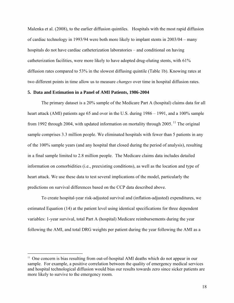
Malenka et al. (2008), to the earlier diffusion quintiles. Hospitals with the most rapid diffusion

of cardiac technology in 1993/94 were both more likely to implant stents in 2003/04 – many

hospitals do not have cardiac catheterization laboratories – and conditional on having

catheterization facilities, were more likely to have adopted drug-eluting stents, with 61%

diffusion rates compared to 53% in the slowest diffusing quintile (Table 1b). Knowing rates at

two different points in time allow us to measure changes over time in hospital diffusion rates.

5. Data and Estimation in a Panel of AMI Patients, 1986-2004

The primary dataset is a 20% sample of the Medicare Part A (hospital) claims data for all

heart attack (AMI) patients age 65 and over in the U.S. during 1986 – 1991, and a 100% sample

from 1992 through 2004, with updated information on mortality through 2005. 11 The original

sample comprises 3.3 million people. We eliminated hospitals with fewer than 5 patients in any

of the 100% sample years (and any hospital that closed during the period of analysis), resulting

in a final sample limited to 2.8 million people. The Medicare claims data includes detailed

information on comorbidities (i.e., preexisting conditions), as well as the location and type of

heart attack. We use these data to test several implications of the model, particularly the

predictions on survival differences based on the CCP data described above.

To create hospital-year risk-adjusted survival and (inflation-adjusted) expenditures, we

estimated Equation (14) at the patient level using identical specifications for three dependent

variables: 1-year survival, total Part A (hospital) Medicare reimbursements during the year

following the AMI, and total DRG weights per patient during the year following the AMI as a

11 One concern is bias resulting from out-of-hospital AMI deaths which do not appear in our sample. For example, a positive correlation between the quality of emergency medical services and hospital technological diffusion would bias our results towards zero since sicker patients are more likely to survive to the emergency room.

19

measure of factor inputs.12 These regressions included categorical variables indicating the

presence of seven comorbid conditions, anatomical location of the MI, and full interactions of

each 5-year age bracket, by sex and race. The initial risk-adjustment regression is shown in

Table A.1 along with relevant means of the independent variables for the entire sample, for both

one-year survival and one-year expenditures.

A first look at the data. We begin with summary statistics showing the time-trend in risk

adjusted survival – in other words, the weighted averages of yit across hospitals within each time

period. Figure 1 shows these risk-adjusted one-year survival and one-year expenditures by year.

Survival rose rapidly during the late 1980s and early 1990s (the period of analysis in Cutler et

al., 1998), but since then has flattened out, particularly in the late 1990s, before assuming a more

modest upward trend in the 2000s.13 And while the 1997 Balanced Budget Act legislation led to

a pause in the rapid cost growth, expenditures have since resumed their upward trend.

We show graphically the bivariate association between technology adoption and risk-

adjusted survival in Figure 2. These display the weighted average of risk-adjusted one-year

survival (yit) by year and by quintile of our diffusion index (the common factor described in

Section 4). The average gap in survival between the slowest and most rapid adopters is more

than 3 percentage points, with the difference widening to 3.5 percent by 2004. The magnitude of

these differences are similar to the estimates we suggested in Section 4 based on what clinical

12 For example, an AMI patient fitted with a drug-eluting stent would qualify for 3.12 DRG “units” in 2003, and this was common across all hospitals. Note that DRG weights may change slightly over time. 13 What can explain this pattern of diminishing returns to technology after the mid-1990s? One possibility is that by this time, aspirin had largely diffused across all patients, and while stents grew also during this period, they “have not been associated with important reductions in mortality.” (Brody, et al, 2003, p. 777) But it is less clear why beta blockers, which were diffusing during this period, didn’t lead to more improvement in outcomes; Masoudi et al. (2006) suggested a secular decline in “ideal” patients for such treatments.

20

trials imply would result from the difference between quintiles in the use of aspirin, beta

blockers, and reperfusion. The lag in terms of years between the most rapid and slowest hospital

adopters varies over the time period, but the average annual (horizontal) gap is roughly ten years,

which is again within the range predicted by the diffusion calculations above.

Figure 3a displays Medicare reimbursements again by quintile of adoption. There are

modest differences in expenditures, with Quintile 5, the most rapidly adopting hospitals,

consistently higher. However, this difference is based primarily on higher reimbursement rates

rather than more inputs per se. Figure 3b shows no difference in expenditures by quintile using a

normalized “price” per DRG weight based on the national average. In sum, there are large long-

run differences in total factor productivity across hospitals, and these do not appear to be

associated with higher rates of factor inputs.

Estimates of the productivity parameter. Table 2 presents estimates of the regression

model in Equation (13). We begin with the simplest regression model in which survival is a

function of the continuous diffusion index, log DRG inputs, and a linear time trend. The

coefficient on the diffusion index is 0.017 (s.e., 0.001). Recall that the diffusion index is an

estimate of a common factor that is proportional to the diffusion rate in each hospital, but

normalized to have a standard deviation of one. Thus, the coefficient implies that a one standard

deviation increase in the diffusion rate is associated with a 1.7 percentage point increase in

patient survival – or has approximately the same impact as doubling DRG inputs (e.g.,

ln(2)*.031=.021, or 2.1%). Adding year effects (Column 2) has little impact on the coefficient.

Columns 3 and 4 replace the continuous diffusion index with dummies for the hospital-specific

diffusion quintile, with Quintile 1 (the slowest diffusion quintile) serving as the reference

category. The coefficient on Quintile 5 relative to Quintile 1 is 0.033 (s.e. 0.002), implying that

survival for hospitals in the fastest diffusion quintile was 3.3 percentage points higher than

21

hospitals in the slowest quintile. This difference in survival corresponds to the fastest quintile

being 11 years ahead of the slowest quintile (the coefficient on the linear trend estimates that the

annual survival improvement was 0.3 percentage points). Again, the differences between

Quintiles 1 and 5 are within the range predicted by the diffusion calculations in Section 4.

Estimates of β, the marginal productivity of factor inputs. Table 3 examines how the

specification of the model affects estimates of β, and interprets them in the context of the cost-

effectiveness ratio. Column (A) of the table reports specifications that do not include year

effects. These regressions are in the spirit of Cutler et al. (1998) who relied solely on variation

over time to identify the average impact of changes in both technology and factor inputs on

survival. In the upper-left corner, we first consider the coefficient estimates from regressions of

survival just on log expenditures, without controlling for technology or year. The coefficient on

log of expenditures, 0.028, is highly significant and implies a cost-effectiveness ratio of

$177,000. The second row, which uses log DRG inputs, delivers a much larger estimate of

0.076, implying a far more favorable cost-effectiveness ratio of $65,000 per life-year. The

bottom two rows suggest diminishing returns to factor inputs over time; the estimated β is larger

in the earlier period (1986-94) than the later period (1995-2004). The cost-effectiveness ratio in

the earlier period is $41,000, which is similar to that obtained by Cutler et al. (1998) using data

from this period.

However, once one introduces year effects – the second column of Rows 1 and 2 – the

coefficient becomes negative (for expenditures) or 0.014 (when using DRGs as factor inputs),

implying at best a cost-effectiveness ratio of $355,000. By controlling for year effects, one ends

up with the small or negative cross-sectional correlations found in Fisher et al. (2003) and

Baicker and Chandra (2004). The final column, using lagged expenditures, finds an even more

negative relationship between factor inputs and survival.

22

Note, however, that the specifications in the first two rows of Table 3 could be biased

because they omitted any control for technological adoption. As we control successively more

for the influence of technological adoption, the coefficient estimates for β rise, and the cost-

effectiveness estimate declines. For example, for the specifications in column (b) that include

year effects, introducing the linear diffusion parameter increases the coefficient from 0.014 to

0.019 (a cost-effectiveness ratio of $261,000) and the quintiles of diffusion yields similar results,

with a coefficient of 0.020. Finally, as shown in Row 5, including hospital fixed effects (which

potentially capture additional differences across hospitals in diffusion not measured by our

diffusion index) raises the estimate of β to 0.052, with an implied cost-effectiveness ratio of

$95,000.

This pattern of coefficients is consistent with our model if the return to factor inputs is

lower in hospitals with higher technology diffusion, as represented graphically in Figure 4 for a

given year. Consider just two hospitals, given by A (on the production function PF(1)) and B (on

the production function PF(2)). If the researcher does not control for technology adoption, she

would estimate the dotted line connecting points A and B – effectively, “flat of the curve” health

care, as shown in Row 1 or 2 of Table 3. As we control with more accuracy for each hospital’s

technology level the estimated (marginal) slope of the production function becomes steeper, to

approximate aa’ or bb’ in Figure 4.

As mentioned in Section 3, year-to-year sampling fluctuations in both factor inputs and

survival may cause an upward bias in estimated β when people who live longer account for more

costs. Limiting the sample to hospitals with more than 50 AMI patients (not reported in Table 3)

implied a cost-effectiveness of $160,000 instead of $95,000 (for a specification with hospital

fixed effects) – still not “flat of the curve.” Alternatively, we also estimated models using lagged

23

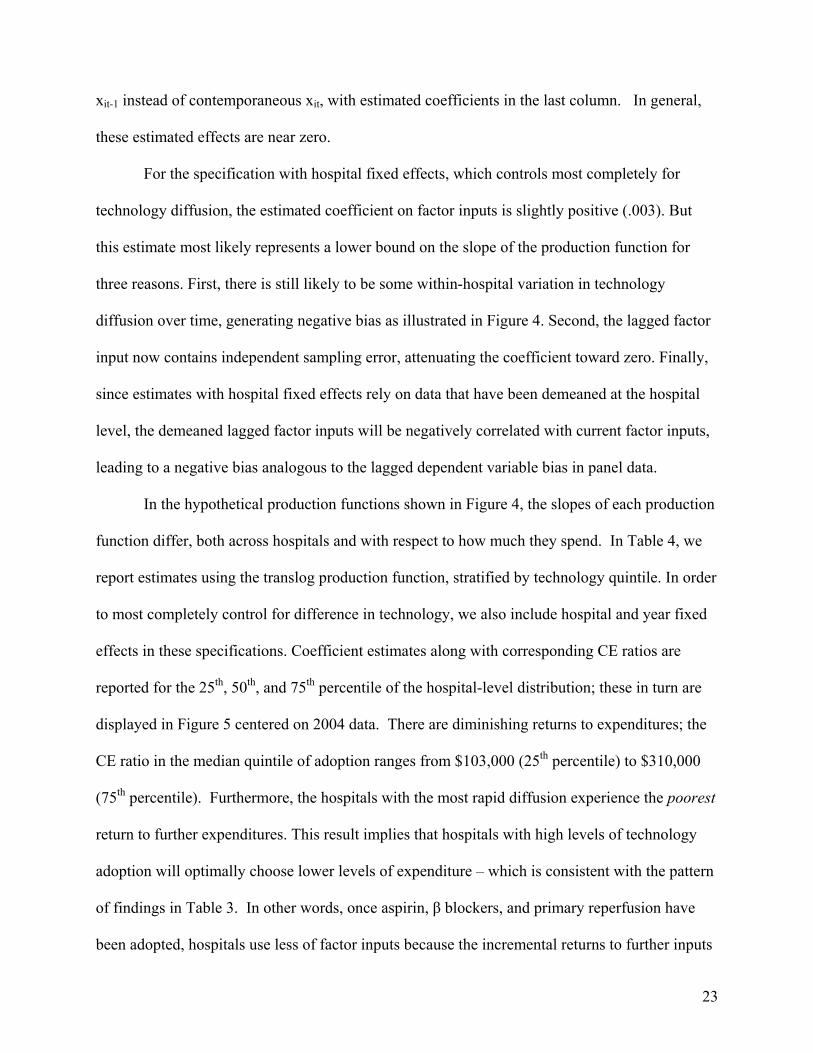
xit-1 instead of contemporaneous xit, with estimated coefficients in the last column. In general,

these estimated effects are near zero.

For the specification with hospital fixed effects, which controls most completely for

technology diffusion, the estimated coefficient on factor inputs is slightly positive (.003). But

this estimate most likely represents a lower bound on the slope of the production function for

three reasons. First, there is still likely to be some within-hospital variation in technology

diffusion over time, generating negative bias as illustrated in Figure 4. Second, the lagged factor

input now contains independent sampling error, attenuating the coefficient toward zero. Finally,

since estimates with hospital fixed effects rely on data that have been demeaned at the hospital

level, the demeaned lagged factor inputs will be negatively correlated with current factor inputs,

leading to a negative bias analogous to the lagged dependent variable bias in panel data.

In the hypothetical production functions shown in Figure 4, the slopes of each production

function differ, both across hospitals and with respect to how much they spend. In Table 4, we

report estimates using the translog production function, stratified by technology quintile. In order

to most completely control for difference in technology, we also include hospital and year fixed

effects in these specifications. Coefficient estimates along with corresponding CE ratios are

reported for the 25th, 50th, and 75th percentile of the hospital-level distribution; these in turn are

displayed in Figure 5 centered on 2004 data. There are diminishing returns to expenditures; the

CE ratio in the median quintile of adoption ranges from $103,000 (25th percentile) to $310,000

(75th percentile). Furthermore, the hospitals with the most rapid diffusion experience the poorest

return to further expenditures. This result implies that hospitals with high levels of technology

adoption will optimally choose lower levels of expenditure – which is consistent with the pattern

of findings in Table 3. In other words, once aspirin, β blockers, and primary reperfusion have

been adopted, hospitals use less of factor inputs because the incremental returns to further inputs

24

such as surgery are modest, a result also found in the clinical literature (Stukel, Lucas, and

Wennberg, 2005). And like Hall and Jones (1999), the rate of technology diffusion explains far

more variation in survival outcomes across hospitals than variations in factor inputs.

Convergence. As noted above, a key implication of the model is the lack of convergence;

the low-diffusion hospitals are predicted to grow at the same rate as high-diffusion hospitals.

This can be seen visually in Figure 2 by noting that the range of Quintile 1 and Quintile 5 is not

narrowing; if anything the range is widening. But we can also test another implication of the

model: that the hospital-level variance in risk-adjusted survival is not predicted to narrow over

time (σ-convergence). We do not find evidence of such convergence: our estimate of the

(weighted) standard deviation of hospital fixed effects, correcting for estimation error, is 0.043 in

1986 and 0.042 in 2004. 14

Changes over time in diffusion rates. A prediction of the theoretical model is that

hospitals which manage to improve their diffusion parameters will, like countries such as Japan

or Korea in the postwar period, experience rapid growth in outcomes (Parente and Prescott,

2002), and conversely. Table 4 further considers risk-adjusted survival among hospitals which

were initially in the slowest diffusion quintile (1) or the highest diffusion quintile (5) during

1994/95. For the slow-diffusion hospitals in 1994/95 remaining a slow diffusion hospital (in

drug-eluting stents) in 2003/04, one-year survival rates rose from 64.5 percent in 1994/95 to 68.8

percent in 2003/04; an increase of 3.7 percent. Similarly, hospitals initially in the highest

diffusing quintile (5) in 1993/94 which remained in the highest diffusing quintile by 2003/04,

14 The correction is done by subtracting the average variance due to estimation error in the hospital fixed effects (the “noise” component). The estimation variance for each hospital’s fixed effect is equal to σ2/Nh, where σ2 is the variance of the error in the patient-level risk-adjustment equation and Nh is the number of AMI patients at hospital h.

25

increased survival by 3.1 percentage points – very similar to the stable low-quintile hospitals, as

predicted by the model.

Hospitals initially in the lowest diffusion quintile during 1994/95 but which moved up to

the highest diffusion quintile for drug-eluting stents in 2003/04 (the “tigers”) experienced a gain

of 5.5 percentage points. By contrast, the hospitals experiencing a decline in diffusion rates from

quintile 5 in 1994/95 to quintile 1 in 2003/04 (the “turtles”) showed a survival gain of just 1.8

percentage points, significantly below those of the “tiger” hospitals.15 Thus, observed changes in

technology diffusion are strongly related to changes in hospital productivity as measured by

patient survival.

5. Conclusion

In this paper, we have attempted to peer inside the black box of hospital productivity

changes both over time and across hospitals. We found that varying rates of adoption for low-

cost but highly effective treatments explained a large fraction of the persistent differences in risk-

adjusted survival during the period 1986-2004. The hospital quintile with the most rapid

propensity to adopt these new innovations experienced survival rates 3.3 percentage points above

the lowest quintile hospitals, or nearly one-third the entire improvement in survival since 1986.

While we focused on just three innovations at a point in time, aspirin, beta blockers, and

reperfusion in 1994/95, we view the results, and the non-convergence of the quintile outcomes,

as supportive of the view that these hospitals have continued to innovate since then. Indeed, the

“tiger” hospitals, those which increased their diffusion rates for new innovations, experienced far

15 One hypothesis is that hospitals that were early adopters of surgery in 1994/95 would also be early adopters of drug-eluting stents in 2003/04, and so the improved survival of the “tiger” hospitals was simply the consequence of surgical innovations paying off in the 2000s. However, drug-eluting stents were no more correlated with surgical procedure rates in 1994/95 than beta blockers or aspirin in 1994/95. Note also that the baseline risk-adjusted survival rates for the stable hospitals were similar to those for the hospitals which subsequently moved (either up or down), lessening a potential concern that selection bias drives these results.

26

more rapid growth in survival outcomes between 1994/95 and 2003/04 than did the “turtle”

hospitals whose speed of diffusion slipped from the highest to the lowest quintile.

Our model of health care productivity reconciles both the dramatic improvements in life

expectancy for AMI patients over time (e.g., Cutler, 2004) and the apparent “flat of the curve”

inefficiencies at a point in time (Fisher et al. 2003). Much of the dramatic growth in survival

occurred as remarkably cost-effective treatments diffused across hospitals during the past few

decades. For example, Ford et al. (2007) found the single most important factor reducing the

number of AMI-related deaths between 1980-2000 was the increased use of aspirin, followed by

beta blockers and ACE Inhibitors (pharmaceutical treatments to reduce hypertension).

But at a point in time, it might appear that greater levels of factor inputs did not result in

improved outcomes. We argue that, at least in the treatment of heart attacks, this “flat of the

curve” association between factor inputs and outcomes may be more apparent than real, arising

because we have not adequately controlled the diffusion parameters that largely determine

hospital productivity. Furthermore, we find the marginal productivity of factor inputs is higher

in the low adoption hospitals, suggesting that the high-cost factor inputs may be substitutes for

the low-cost innovations (Chandra and Staiger, 2007). Of course, these estimates are sensitive to

the specification of the model, so we cannot rule out “flat of the curve” spending entirely,

particularly for the higher-intensity hospitals. Nor do these results necessarily apply for the

treatment of diseases other than heart attacks, where technological gains have been far less

prevalent.

There are a variety of optimizing economic models where rational agents adopt slowly

because they are waiting for the price to decline (e.g., flat-screen TVs), or because of expertise in

the older technology (Jovanovic and Nyarko, 1996). Alternatively, heterogeneity in production

functions may lead to profit-maximizing differences in rates of diffusion (Griliches, 1957), or the

27

presence of liquidity constraints may slow diffusion (Suri, 2006). Finally, there may be

differences in education across workers which affect their propensity to adopt (Nelson and

Phelps, 1966) or technology may be most complementary with skilled workers (Caselli and

Coleman, 2006). None of these models provides a good explanation of the non-adoption of

inexpensive beta blockers, aspirin, and reperfusion by highly educated physicians. 16

Because prices do not play an important role here, we instead look to informational or

search barriers as an explanation for why physicians don’t adopt. Recall Equation (11) which

posited a first-order condition in which the marginal cost of speeding up diffusion C’(π), was set

equal to the marginal benefit of innovating more rapidly. Using plausible parameters for

measuring the social value of more rapid adoption yields a very high cognitive barrier: the

implicit cost facing each physician of moving up just one diffusion quintile must be $11,200

annually. 17 Alternatively, the implicit value placed by hospitals and physicians on a life-year

must be well below $25,000 per life-year to generate “reasonable” equilibrium conditions to

explain observed slow diffusion rates.

One might also appeal to models of social norms to explain why innovations diffuse more

rapidly in some regions than others, whether hybrid corn in the 1930s and 1940s or beta blockers

in the 2000s (Skinner and Staiger, 2007), but the direction of causality is not well understood.

The quality of management, including staff “opinion leaders,” is clearly central to the rapid

diffusion of beta blockers (Bradley, et al., 2001, 2005). Thus the diffusion parameters could as

well be symptomatic of managerial efficiency, which has shown in non-health industries to be an

16 The distinction between “inefficient” barriers to adoption, and the slow, but optimal, adoption of technology for a variety of reasons, was made by Coleman (2004). 17 We assume that the average lag from the frontier, at* - at = 0.02, Ψ = $100,000, the one-year survival following AMI translates to an additional 5.25 life-years, r = .05, baseline π = .10, π must increase by 0.016 to shift to the next quintile (one-fifth the range between 6 and 14 percent, the implicit aspirin diffusion rates), and there are 10 AMI patients per physician.

28

important determinant of productivity (Bloom and van Reenan, 2007). But even after accounting

for the lower productivity in hospitals compared to other industries (Bloom, Seiler, and van

Reenan, 2007), one is still left with a puzzle of why individual physicians need management or

opinion leaders to convince them to adopt aspirin for their heart attack patients.

Leibenstein (1966) used the term “X-efficiency” to describe residual differences in firm-

level productivity which could not be readily explained by measured inputs or other factors. In

many respects, the puzzle of slow diffusion for efficient AMI treatments provides a textbook

case of X-inefficiency, because here at least we can observe directly several productivity

measures rather than infer them as residuals, as Leibenstein did. While informational barriers are

indeed important –there may be no one in the hospital to provide the “tactile” learning when

reading an article just isn’t enough (Keller, 2004) – there has historically been little pressure

exerted by markets or management to change old habits and adopt the new innovations. It is

telling that the increased public hospital-level reporting of beta blocker use for AMI patients has

been central to its nearly universal diffusion in the last decade (Lee, 2007).

Parente and Prescott (2002) provide a ready explanation for why some countries lag so

far behind “frontier” countries: government restrictions and monopoly restraints that interfere

with the benefits of efficient technology adoption. Health care markets are notoriously

imperfect. If patients both knew about the benefits of aspirin, beta blockers, and reperfusion, and

were sensitive to published and reliable information about hospital quality, physicians would be

forced to respond rapidly to new innovations or face the loss of patients. But when quality

measures are limited, patients are not well informed, and markets are distorted, remarkably large

inefficiencies can persist across hospitals and over time.

29

References

Baicker, Katherine and Amitabh Chandra, “Medicare Spending, The Physician Workforce, and The Quality Of Health Care Received By Medicare Beneficiaries.” Health Affairs, April 2004: 184-97. Berndt, Ernst R., Anupa Bir, Susan H. Busch, Richard G. Frank and Sharon-Lise T. Normand, "The Medical Treatment of Depression, 1991-1996: Productive Inefficiency, Expected Outcome Variations and Price Indexes," Journal of Health Economics, 21(3), 2002: 373-396, Bero, Lisa A., Roberto Grilli, Jeremy M. Grimshaw, et al., “Closing the Gap Between Research and Practice: An Overview of Systematic Reviews of Interventions to Promote the Implementation of Research Findings,” BMJ 317, August 15, 1998: 465-468. Berwick, Donald M., “Disseminating Innovations in Health Care,” JAMA 289(15), April 16, 2003: 1969-1975. Bloom, Nicholas, and John Van Reenen, "Measuring and Explaining Management Practices Across Firms and Countries," Quarterly Journal of Economics, November 2007: 1351-1408. Bloom, Nicholas, Stephan Seiler, and John Van Reenen, "Management Matters in Health Care," Working Paper, London School of Economics, November 2007. Bradley, Elizabeth H., Eric S. Holmboe, Jennifer A. Mattera. et al., “A Qualitative Study of Increasing β-Blocker Use After Myocardial Infarction: Why Do Some Hospitals Succeed?,” JAMA 285(20), 2001: 2604-2611. Bradley, Elizabeth H., Jeph Herrin, Jennifer A. Mattera, Eric S. Holmboe, Yongfei Wang, et al., “Quality Improvement Efforts and Hospital Performance: Rates of Beta-Blocker Prescription After Acute Myocardial Infarction,” Medical Care, 43(3), March 2005: 282-92. Caselli, Francesco, and Wilbur John Coleman II, “The World Technology Frontier,” American Economic Review 96(3), June 2006: 499-522. Chandra, Amitabh, and Douglas Staiger, “Testing a Roy Model with Productivity Spillovers: Evidence from the Treatment of Heart Attacks,” Journal of Political Economy, February 2007. Coleman, Wilbur John II, “Comment on ‘Cross-Country Technology Adoption: Making the Theories Face the Facts,” Journal of Monetary Economics 51, 2004: 85-87. Comin, Diego, and Bart Hobijn, “Cross Country Technology Adoption: Making the Theories Face the Facts,” Journal of Monetary Economics 51, 2004: 39-83. Comin, Diego, and Bart Hobijn, "An Exploration of Technology Diffusion," mimeo, Federal Reserve Bank of San Francisco, October 2008.

30

Christensen, Laurits R., Dale W. Jorgenson, Lawrence J. Lau, "Transcendental Logarithmic Production Frontiers," The Review of Economics and Statistics, 55(1) February 1973: 28-45. Crespi, Gustavo, Chiara Criscuolo, Jonathan E. Haskel, and Matthew Slaughter, Productivity Growth, Knowledge Flows, and Spillovers," NBER Working Paper No. 13959, April 2008. Cutler, David M., Mark McClellan, Joseph P. Newhouse, and Dahlia Remler, “Are Medical Prices Declining? Evidence from Heart Attack Treatments,” Quarterly Journal of Economics 93(4) 1998: 991-1024. Cutler, David M. Your Money or Your Life: Strong Medicine for America’s Health Care System. New York: Oxford University Press, 2004. Eaton, Jonathan, and Samuel Kortum, “International Technology Diffusion: Theory and Measurement,” International Economic Review, 40(3), August 1999: 537-570. Enthoven, Alan C., “Shattuck Lecture—Cutting Cost without Cutting the Quality of Care,” New England Journal of Medicine 298(22) 1978: 1229–1238. Fisher, Elliott S., David Wennberg, Therese Stukel, Daniel Gottlieb, F.L. Lucas, and Etoile L. Pinder, "The Implications of Regional Variations in Medicare Spending. Part 2: Health Outcomes and Satisfaction With Care" Annals of Internal Medicine 138(4), February 18, 2003: 288-299. FTT (Fibrinolytic Therapy Trialists' Collaborative Group), "Indications for Fibrinolytic Therapy in Suspected Acute Myocardial Infarction: Collaborative Overview of Early Mortality and Major Morbidity Results from All Randomised Trials of More than 1000 Patients. Fibrinolytic Therapy Trialists' (FTT) Collaborative Group," Lancet 343(8893), Feb 5, 1994:311. Ford, Earl S., Umed A Ajini, Janet B. Croft, et al., "Explaining the Decrease in U.S. Deaths from Coronary Disease, 1980–2000," NEJM 356, June 7, 2007: 2388-2398. Fuchs, Victor R., "More Variation In Use Of Care, More Flat-Of-The-Curve Medicine," Health Affairs, October 7, 2004 Web Exclusive. Griliches, Zvi, “Hybrid Corn: An Exploration in the Economics of Technological Change,” Econometrica 25(4) (October 1957): 501-522. Hall, Bronwyn, “Innovation and Diffusion,” in Jan Fagerberg, David C. Mowery, and Richard R. Nelson, Handbook on Innovation. Oxford: Oxford University Press (2004). Hall, Robert E., and Charles I. Jones, "Why Do Some Countries Produce So Much More Output Per Worker Than Others?" Quarterly Journal of Economics, 114(1) February 1999: 83-116. Hall, Robert, and Charles I. Jones, 2007. “The Value of Life and the Rise in Health Spending,” Quarterly Journal of Economics, 122(1):39-72.

31

Heidenreich, PA, and M McClellan, “Trends in Treatment and Outcomes for Acute Myocardial Infarction: 1975-1995.” The American Journal of Medicine 110(3), 2001: 165-174. Hirth, Richard A., Michael E. Chernew, Edward Miller, A. Mark Fendrick, and William G. Weissert, "Willingness to Pay for a Quality-Adjusted Life Year: In Search of a Standard," Medical Decision Making, 20(3), 2000:332-342. Horwitz, Jill, and Austin Nichols, “What do Nonprofits Maximize? Nonprofit Hospital Service Provision and Market Ownership Mix,” NBER Working Paper No. 13246, July 2007. ISIS-2: The Second International Study of Infarct Survival Collaborative Group, “Randomised Trial of Intravenous Streptokinase, Oral Aspirin, Both, or Neither among 17,187 Cases of Suspected Acute Myocardial Infarction: ISIS-2,” Lancet 32(8607), 1988: 349–360. Jacobs, Rowena, Peter C. Smith, and Andrew Street, Measuring Efficiency in Health Care: Analytic Techniques and Health Policy. New York: Cambridge University Press, 2006. Jencks, Stephen F., Edwin D. Huff, and Timothy Cuerdon, “Change in the Quality of Care Delivered to Medicare Beneficiaries, 1998-99 to 2000-2001,” JAMA 289(3) (January 15, 2003): 305-312. Jovanovic, Boyan, and Yaw Nyarko, “Learning by Doing and the Choice of Technology,” Econometrica 64(6) (November 1996): 1299-1310. Keller, Wolfgang, “International Technology Diffusion,” Journal of Economic Literature 42(3), 2004, 752-82. King, Joseph T. Jr., Joel Tsevat, Judith R. Lave, and Mark S. Roberts, "Willingness to Pay for a Quality-Adjusted Life Year: Implications for Societal Health Care Resource Allocation," Medical Decision Making, 25(6), 2005: 667-677. Krumholz HM, Radford MJ, Ellerbeck EF, et al., "Aspirin in the treatment of acute myocardial infarction in elderly Medicare beneficiaries. Patterns of use and outcomes," Circulation 92(10), November 15, 1995: 2841-7. Lee, Thomas H., "Eulogy for a Quality Measure," New England Journal of Medicine, 357(12), September 20, 2007: 1175-77. Lee, Jong-Wook, “Health Challenges for Research in the 21st Century,” WHO David Barnes Global Health Lecture, Bethesda, Maryland, December 6, 2004. http://www.who.int/dg/lee/speeches/2004/barmeslecture/en/ (Accessed March 12, 2007). Leibenstein, Harvey, “Allocative Efficiency vs. ‘X-efficiency’,” American Economic Review, 56, 1966: 392-415.

32

Malenka, David .J., Aaron .V. Kaplan, Lee Lucas, Sandra. M Sharp, Jonathan S. Skinner, "Outcomes Following Coronary Stenting in the Era of Bare Metal versus the Era of Drug Eluting Stents," JAMA 299(24), June 25, 2008: 2868-2876. Masoudi, Fredrick A., JoAnne M. Foody, Edward P. Havranek, Yongfei Wang, Martha J. Radford, et al., "Trends in Acute Myocardial Infarction in 4 US States Between 1992 and 2001: Clinical Characteristics, Quality of Care, and Outcomes," Circulation 114, December 19/26, 2006: 83-116. Murphy, Kevin M. and Topel, Robert H., "The Value of Health and Longevity," Journal of Political Economy 114(5) October 2006: 871-904. Nelson, Richard R., and Edmund S. Phelps, "Investment in Humans, Technological Diffusion, and Economic Growth," American Economic Review 56(2), May 1966: 69-75. Parente, Stephen L. , and Edward C. Prescott, "Barriers to Technology Adoption and Development,"The Journal of Political Economy 102(2), April 1994: 298-321. Parente, Stephen L., and Edward C. Prescott, Barriers to Riches. Cambridge: MIT University Press, 2002. Phelps, Charles E., “Information Diffusion and Best Practice Adoption,” in A.J. Culyer and J.P. Newhouse (eds.) Handbook of Health Economics Volume 1, Elsevier Science (2000): 223-264. Phillips, Kathryn A., Micheal G. Shlipak, Pam Coxson, et al., “Health and Economic Benefits of Increased β Blocker Use Following Myocardial Infarction,” JAMA, 284(21), December 6, 2000: 2748-2754. Rogers, E.M. Diffusion of Innovations. (5th Edition.) New York: The Free Press (2003). Skinner, Jonathan, Elliott Fisher, and John E. Wennberg, “The Efficiency of Medicare” in David Wise (ed.) Analyses in the Economics of Aging. Chicago: University of Chicago Press and NBER, 2005:129-57. Skinner, Jonathan, and Douglas Staiger, "Technological Diffusion from Hybrid Corn to Beta Blockers,” in E. Berndt and C. M. Hulten (eds.) Hard-to-Measure Goods and Services: Essays in Honor of Zvi Griliches. University of Chicago Press and NBER 2007. Stukel, Therese A., F. Lee Lucas, and David E. Wennberg, "Long-term Outcomes of Regional Variations in Intensity of Invasive vs. Medical Management of Medicare Patients with Acute Myocardial Infarction," JAMA, 293, 2005:1329-1337. Suri, Tavneet, “Selection and Comparative Advantage in Technology Adoption”, MIT, January 2008.

33

Yusuf S., Peto R., Lewis J., Collins R., Sleight P. “Beta blockade during and after myocardial infarction: an overview of the randomized trials,” Progress in Cardiovascular Diseases. 1985;27(5):335-71.

34

Table 1a: Characteristics of Factor Model of Adoption: Correlation Structure

Common

Factor Aspirin β Blocker Reperfusion

Common Factor

Aspirin 0.871*

β Blocker 0.792*

0.429*

12 Hour Reperfusion

0.300*

0.189*

0.031

Notes: The table reports correlations at the hospital level (N = 2765) weighted by number of patients in each hospital. Data from the Cooperative Cardiovascular Project (CCP), 1994/95, with a sample of 139,847 AMI patients. * denotes p < 0.001

Table 1b: Characteristics of Factor Model of Adoption: Association with Characteristics of the Hospital

Quintile 5 (Quickest)

Quintile 4 Quintile 3 Quintile 2 Quintile 1 (Slowest)

Overall

Aspirin 0.90 0.85 0.80 0.76 0.65 0.80 β Blocker 0.65 0.53 0.46 0.40 0.31 0.47 Reperfusion within 12 hours 0.21 0.20 0.19 0.18 0.15 0.18

Average hospital volume* 95 101 94 88 67 89

Major teaching hospital 0.43 0.30 0.23 0.17 0.05 0.24

Average State Income (1994/95) 43,790 42,603 42,168 42,215 41,648 42,495

% Admitted to Hospital Performing Stents in 2003 /04

0.73 0.70 0.60 0.50 0.31 0.57

Of those, % Drug-Eluting Stent 2003/04 0.61 0.62 0.39 0.55 0.53 0.59

See notes above in Table 1a. *Volume for Medicare patients only. Weighted by number of patients in each hospital. Estimates for each quintile are based on samples of approximately 28,000 AMI patients. Stent data are derived from Medicare Part A (hospital) claims.

35

Table 2: Regression Estimates of Survival on Technology Diffusion and

Factor Inputs Notes: N = 49,937 hospital-years. All regression weighted by the number of patients in each hospital-year. Sample limited to hospital/year observations with at least 5 observations per hospital. Standard errors (clustered at the hospital level) in parentheses.

Input 1 2 3 4 Diffusion

(continuous) 0.017

(0.001) 0.017

(0.001)

Diffusion Quintile 2 0.012

(0.002) 0.012

(0.002) Diffusion Quintile 3 0.020

(0.002) 0.020

(0.002) Diffusion Quintile 4 0.028

(0.002) 0.028

(0.002) Diffusion Quintile 5 0.033

(0.002) 0.033

(0.002)

Log (DRG) 0.031 (0.004)

0.019 (0.004)

0.031 (0.004)

0.020 (0.004)

Year Trend 0.0030 (0.0001)

Fixed effects

0.0030 (0.0001)

Fixed effects

36

Table 3: Regression Estimates of Survival on Factor Inputs for Alternative Specifications

Notes: See notes to Table 2. Each entry in the table is the coefficient on factor inputs from a different specification as indicated in the table. Models with lags drop data from 1986, and have N=46,098. Cost-effectiveness ratios in brackets.

Input Period of

Analysis

Adj. for Diffusion

(A) No Year Effects

(B) Year Effects

(C) Year Effects Lagged Input

1 Log(Expend) 86-04 No 0.028

(0.002) [$177,000]

-0.010 (0.003)

[Undefined]

-0.015 (0.003)

[Undefined]

2 Log(DRG) 86-04 No 0.076

(0.003) [$65,000]

0.014 (0.004)

[$355,000]

-0.015 (0.004)

[Undefined]

3 Log(DRG) 86-04 Continuous Measure

0.078 (0.003)

[$64,000]

0.019 (0.004)

[$261,000]

-0.010 (0.003)

[Undefined]

4 Log(DRG) 86-04 Diffusion Quintile

0.078 (0.003)

[$64,000]

0.020 (0.004)

[$248,000]

-0.010 (0.003)

[Undefined]

5 Log(DRG) 86-04 Hospital

Fixed Effect

0.102 (0.002)

[$49,000]

0.052 (0.003)

[$95,000]

0.003 (0.003)

[>$1 mill.]

6 Log(DRG) 86-94 Hospital

Fixed Effect

0.122 (0.004)

[$41,000]

0.068 (0.004)

[$73,000]

-0.004 (0.004)

[Undefined]

7 Log(DRG) 95-04 Hospital

Fixed Effect

0.047 (0.004)

[$106,000]

0.043 (0.004)

[$115,000]

0.002 (0.004)

[>$1 mill.]

37

Table 4: Regression Estimates Stratified by Quintile of Diffusion

Coefficient Ln(DRG)

CoefficientLn(DRG)2

CE Ratio: 25th

Percentile

CE Ratio: 50th

Percentile

CE Ratio: 75th

Percentile

Quintile 1 (Slowest)

N = 13,968

0.233 (0.033)

-0.060 (0.011)

0.071 (0.006)

[$70,000]

0.057 (0.006)

[$87,000]

0.045 (0.007)

[$110,000]

Quintile 2 N = 10,132

0.214 (0.038)

-0.058 (0.014)

0.058 (0.007)

[$86,000]

0.045 (0.007)

[$110,000]

0.032 (0.009)

[$155,000]

Quintile 3 (Middle) N = 8,923

0.243 (0.037)

-0.073 (0.013)

0.048 (0.006)

[$103,000]

0.031 (0.007)

[$160,000]

0.016 (0.008)

[$310,000]

Quintile 4 N = 8,183

0.219 (0.043)

-0.061 (0.016)

0.053 (0.057)

[$94,000]

0.039 (0.008)

[$127,000]

0.026 (0.009)

[$191,000]

Quintile 5 (Fastest)

N = 8,731

0.259 (0.038)

-0.080 (0.014)

0.044 (0.007)

[$113,000]

0.025 (0.007)

[$199,000]

0.009 (0.009)

[$552,000]

Notes: See notes to Table 2. Each row reports results from estimating a regression of survival on ln(DRG) and ln(DRG)2, controlling for hospital and year fixed effects. Cost-effectiveness ratios in brackets.

38

Table 5: Growth in Risk-Adjusted Survival by Diffusion Quintiles in 1994/95 and in 2003

Survival: 1994/95 Survival: 2003/04 Change in Survival:

1994/95 to 2003/04

2003/04 Quintile 1 (Slowest)

2003/04 Quintile 5 (Fastest)

2003/04 Quintile 1 (Slowest)

2003/04 Quintile 5 (Fastest)

2003/04 Quintile 1 (Slowest)

2003/04 Quintile 5 (Fastest)

1994/95 Quintile 1 (Slowest)

0.651 (0.008)

0.656 (0.013)

0.688 (0.004)

0.712 (0.012)

0.037 (0.009)

0.055 (0.015)

1994/95 Quintile 5 (Fastest)

0.684 (0.006)

0.690 (0.005)

0.701 (0.007)

0.721 (0.006)

0.013 (0.008)

0.031 (0.006)

Notes: All standard errors are clustered at the hospital level.

39

Figure 1: One-Year Risk-Adjusted Survival Rate and One-Year Inpatient

(Part A) Hospital Expenditures Following AMI (2004$)

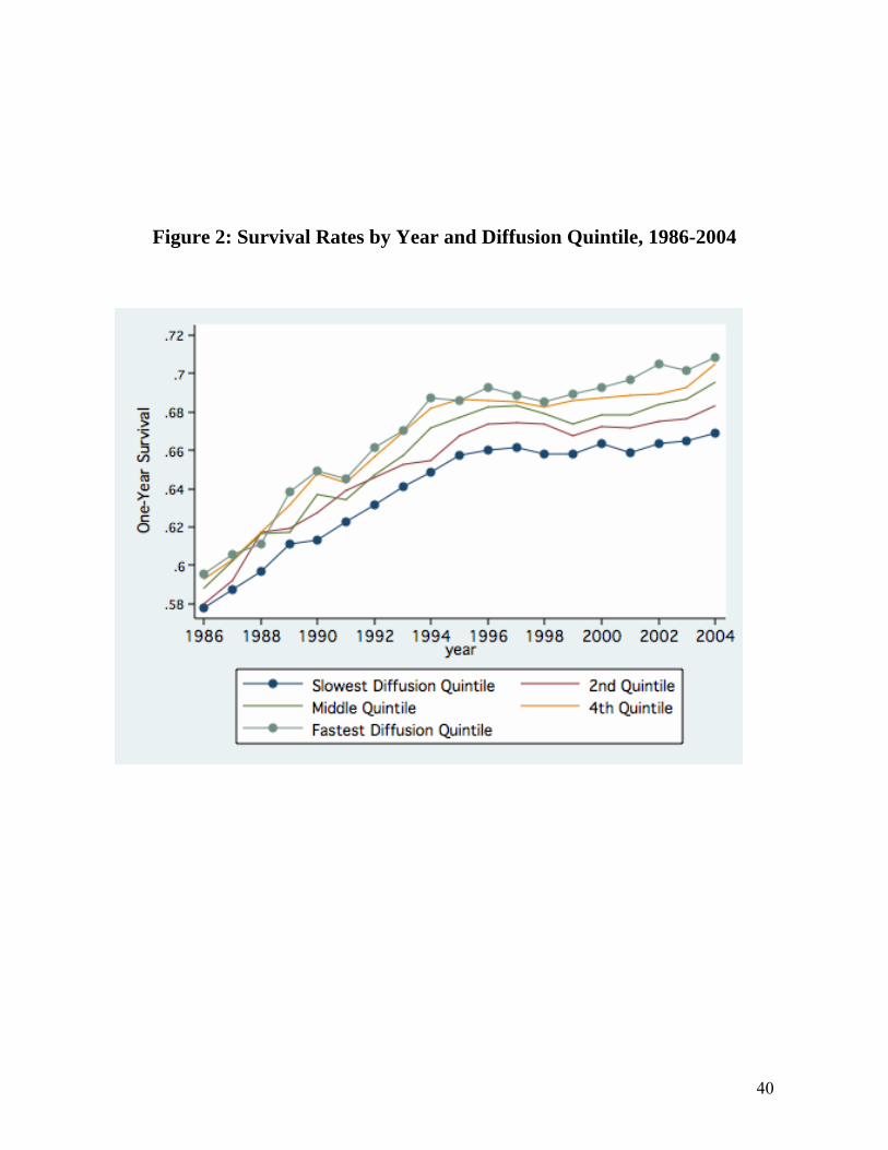
40

Figure 2: Survival Rates by Year and Diffusion Quintile, 1986-2004

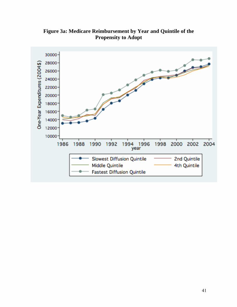
41

Figure 3a: Medicare Reimbursement by Year and Quintile of the Propensity to Adopt

42

Figure 3b: Normalized Medicare Reimbursements (DRG Weights

Multiplied by Common Reimbursement Rate)

43

Figure 4: Interpreting the Evidence on Survival and Health Outcomes: “Flat of the Curve” vs. Productivity Differentials

Factor Inputs

SurvivalPF(1)

0

B

APF(2)

a’

a

b’

b

44

Figure 5: Estimated Production Functions for Quintiles 1 (Fastest) 3

(Middle) and 5 (Slowest) Hospitals, 2004

Note: Estimates based on regression analysis reported in Table 4.

Fastest Middle Slowest

45

Appendix: The Derivation of the Dynamic Model

We rewrite the objective function (7) for hospital i at time t as Equation A.1:

(A.1) [ ] tititiititiititi

ti rKCXPxaV −

∞

=

++−−+Ψ=∑ )1()()(0

πϕβ

The basic model – in which saving lives is good, and spending more is bad – is consistent with a range of models trying to capture what it is that hospitals maximize. For example, consider a model in which there exists a tension between two goals of the hospital: to maximize social welfare – the value of lives saved less resource costs – and the desire to maintain financial stability by maximizing profits. Suppose that the relative weight between the two objectives is given by μi, which is hospital-specific and ranges between one (the hospital maximizes social welfare without regard to its own financial position) and zero (the hospital cares solely about maximizing profit). Thus the objective function is

[ ] titiitititiiitiitititititi

ti rCKXPCKXPxaV −

∞

=

+−+−+−+−+Ψ=∑ )1()]()[1()]()([ *

0πωμπβμ

(A.2)

in which Ψ* is the true social value of survival, ωi the marginal proportional contribution to profitability of an incremental Xit, and Kit , the fixed subsidization or fixed costs, and Pit the factor cost, are defined as above. It is straightforward to show that (A.1) is a “reduced-form” version of (A.2), where Ψi = μi Ψ* and )1( iiii μωμϕ −−= . Note that 0>iϕ for the solution to exist (since the marginal productivity of Xit in this log-linear production function never turns negative), so the temptation to provide a highly profitable procedure must be tempered by at least some desire to curb allocative inefficiency.

The discrete discrete-time Lagrangian based on A.1 is written

(A.3) )]([ *1

01 ittitit

tititi aaaaV −−−−=ℑ +

∞

=+∑ πλ

This model can also be written in continuous time as a current-value Hamiltonian, but we maintain a discrete time structure to help specify the empirical model. The first-order conditions are written:

(A.4a) titi

it

i

it

rPXX

−+⎥⎦

⎤⎢⎣

⎡−

Ψ=

∂∂ℑ )1(ϕ

β

(A.4b) )(')1( *1 ittitit

t

it

aaCr −++−=∂∂ℑ

+− λ

π

(A.4c) 1)1()1( −− −−++Ψ=

∂∂ℑ

itititt

iit

ra

λπλ

46

(A.4d) )( *11 ittititit

it

aaaa −−−=∂∂ℑ

++ πλ

In addition to these four first-order conditions, we also add a solvency constraint:

(A.4e) [ ] 0)1()(0

≥+−Κ+ −∞

=∑ t

itiitititit

rCXP πϕ

to ensure the present value of profits is non-negative (although hospitals can lose money in a given year). While hospitals do go out of business, we seek to avoid these more complicated issues by focusing solely on hospitals that remain in the panel during the period of analysis.

We first characterize the equilibrium, and demonstrate that a steady-state solution exists: πit = πi. To show this, we first solve for λit. Dropping the i subscript and assuming a constant π, (A.3c) is written

(A.5) 110 )1()1( −+Ψ+−= rμπλλ

....)1()1( 2

21−+Ψ+−= rμπλλ

and by progressive substitution:

(A.6) ⎥⎥⎦

⎤

⎢⎢⎣

⎡⎟⎠⎞

⎜⎝⎛

+−

+⎟⎠⎞

⎜⎝⎛

+−

++−

++Ψ+−=−

−12

10 1

1...11

111)1()1(

kk

k rrrr πππμπλλ

Solving for the infinite series (which converges given that π and r > 0) and assuming that the transversality condition is met, so that k

k )1( πλ − converges to zero as k gets large, )/(0 r+Ψ= πλ . From A.5,

11 )1()1( −+Ψ+−=

+Ψ r

rμπλ

π

By successive substitution, )1/(1 rtt += −λλ . This in turn implies a steady-state solution for Xit = Xi (since both λ and the objective function decay at the rate r).

By rearranging A.4b and substituting for λt, one can derive Equation (11) in the text. By further substituting (1-π)/π for (at* - at), which comes from the steady-state expression in Equation (10), we can also write the solution for π as:

(A.7) ⎥⎦⎤

⎢⎣⎡

+−

Ψ=ππ

παπr

C i1)1()('

Simulations of this key first-order condition suggests a high degree of dynamic stability.

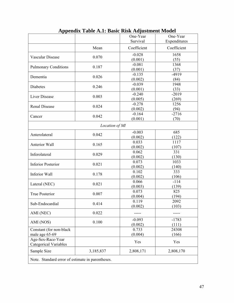
47

Appendix Table A.1: Basic Risk Adjustment Model One-Year

Survival One-Year

Expenditures Mean Coefficient Coefficient

Vascular Disease 0.070 -0.028 (0.001)

1658 (55)

Pulmonary Conditions 0.187 -0.081 (0.001)

1368 (37)

Dementia 0.026 -0.135 (0.002)

-4919 (84)

Diabetes 0.246 -0.039 (0.001)

1948 (33)

Liver Disease 0.003 -0.240 (0.005)

-2019 (269)

Renal Disease 0.024 -0.278 (0.002)

1256 (94)

Cancer 0.042 -0.164 (0.001)

-2716 (70)

Location of MI

Anterolateral 0.042 -0.003 (0.002)

685 (122)

Anterior Wall 0.165 0.033 (0.002)

1117 (107)

Inferolateral 0.029 0.062 (0.002)

331 (130)

Inferior Posterior 0.021 0.073 (0.002)

1033 (140)

Inferior Wall 0.178 0.102 (0.002)

333 (106)

Lateral (NEC) 0.021 0.066 (0.003)

-114 (139)

True Posterior 0.007 0.073 (0.004)

825 (194)

Sub-Endocardial 0.414 0.119 (0.002)

2092 (103)

AMI (NEC) 0.022 ----- -----

AMI (NOS) 0.100 -0.093 (0.002)

-1783 (111)

Constant (for non-black male age 65-69 0.733

(0.004) 24308 (166)

Age-Sex-Race-Year Categorical Variables Yes Yes

Sample Size 3,185,837 2,808,171 2,808,170

Note. Standard error of estimate in parentheses.