Technology Adoption Costs and Productivity Growth: …researchoninnovation.org/qadopt.pdf · 1 –...

Technology Adoption Costs and Productivity Growth:

The Transition to Information Technology

By James Bessen*

10/01

Abstract: Using two panels of U.S. manufacturing industries, this paper estimates capitaladjustment costs from 1961 to 1996. I find that from 1974-83 adjustment costs rose sharply—theymore than doubled from about 3% of output to around 7%. Moreover, this increase is specificallyassociated with a shift to investment in information technology. But such large adoption costsimply that the Solow residual mismeasures productivity growth: adoption costs are resource costsrepresenting an unmeasured investment. I find that when this investment is included, productivitygrew about 0.4% per annum faster than official measures during the 70’s and early 80’s, reducingthe size of the productivity “slowdown.” Indeed, estimated productivity growth rates were roughlythe same from 1974-88 as from 1949-73. Thus technology transitions critically affect productivitygrowth measurement.

Keywords: Technological change, productivity, adjustment cost, information technology

JEL codes: O30, O47, E22

James BessenResearch on [email protected]

*Thanks to Diego Comin, Bob Hunt, Boyan Jovanovic and several referees for helpful comments.Thanks to Randy Becker, Bill Gullickson, Shelby Herman and Steve Rosenthal for data andinformation about data.

1 – Technology Adoption Costs and Productivity Growth - Bessen – 9/01

I. Introduction

The literature on technology adoption is filled with examples of abrupt technology

transitions. For example, U.S. railroads shifted from using mainly steam locomotives to mainly

diesel locomotives in a decade [Mansfield, 1968, p. 175]. The standard technology adoption curve

(“diffusion” curve) is S-shaped—very rapid adoption after a long, slow initial period. Moreover,

with “general purpose technologies” [Helpman, 1998], many different industries may adopt new

technologies at once. For example, many industries adopted electricity-based technologies during

the 1920’s and 30’s and many adopted electronics-based technologies during the 1970’s and 80’s.

Such Schumpeterian technology transitions pose a problem for productivity measurement

because such new technologies are usually new goods, that is, they are not perfect substitutes for

earlier technologies. Specifically, whole new technologies may incur large adoption costs because

they involve learning new skills, implementing new forms of organization, and developing

complementary investments. Indeed, reviewing the recent literature on the impact of computers,

Brynjolfsson and Hitt [2000] find that complementary organizational investments may be much

larger than the investment in computer equipment itself. Also, information technology, in

particular, often involves customization and custom-software, some of which remains unmeasured

in official statistics. Because such complementary investments appear in official productivity

statistics only as resource costs without the corresponding contribution to investment (and hence

output), productivity may be mismeasured.

This paper estimates these adoption costs in the U.S. manufacturing sector from 1961-96

and it calculates revised productivity growth estimates based on these. Using two panels of

industry data (one using 4-digit SIC industries, the other 2-digit), I obtain two main empirical

results. First, I find that capital adjustment costs rose sharply during the period from 1974-83, at

the same time as investment sharply shifted toward information technology (IT). Second, I find that

this rise in costs is specifically associated with this change in technology. In other words, these are

costs of adopting new technology.

Applying adjustment cost estimates from each panel to BLS productivity measures for the

manufacturing sector, I obtain estimates of productivity growth from 1974-83 of 0.91% and

0.94%, compared to an official estimate of 0.52%. For 1974-88 the estimates are 1.42% and

1.53%, compared to 1.13%. These growth rates compare favorably to the official growth measures

from 1949-73 of 1.52%, suggesting that any productivity slowdown was brief at most.


Implications and relationship to the literature

Several studies have presented models where adoption costs account for the productivity

slowdown of the 70’s, including Hornstein and Krusell [1996], Greenwood and Yorukoglu [1997]

and Greenwood and Jovanovic [1998]. In these models, adoption costs are assumed to increase

with the rate of embodied technical change. Several authors, including Gort and Wall [1998],

Greenwood et al [1997], Hercowitz [1998], and Hulten [1992], have also considered the effect of

embodied technical change on productivity measurement during the 70’s and 80’s.

Many of these studies infer a rate of embodied technical change from the slow drift

between official price deflators for producer’s durable equipment and Gordon’s [1990] alternative

estimates. But Gordon’s quality-adjusted price deflators are unlikely to capture the full value of

adoption costs, which are complementary investments.1 And the resulting estimates are

qualitatively quite different. Gordon’s “drift” grows steadily at about 3% a year during the postwar

period. My estimates of adoption costs surge sharply in the 70’s (see Figure 3 below).

Several other studies have used calibrated models to explore adoption costs (or

organizational costs), including Robert Hall [2000] and Michael T. Kiley [1999, 2000]. Again, the

pattern emerging from my direct estimates is generally different.

The magnitude of this acceleration is important not only because it affects the calculation

of productivity growth. Several of these models also relate the rise in adoption costs in the 70’s to

changes in wages, the skill premium and stock prices. For instance, Greenwood and Yorukoglu

speculate that the growth rate of embodied technical change accelerated 2% per annum during the

70’s. From this, their model implies a roughly 1.5% increase in learning costs as a share of GDP

and a substantial increase in wage inequality. Yet my estimates suggest that adoption costs

increased by 4% of GDP in the 70’s. The implied effect on wage inequality, stock prices and other

variables should also be correspondingly larger.

Another literature has attempted to assess the impact of IT on productivity, including

Berndt and Morrison [1995], Chun [2001], Jorgenson and Stiroh [1999, 2000], Oliner and Sichel

[1994, 2000] and Whelan [2000]. This literature suggests that the returns to IT investment were

low or non-existent during the 70’s and early 80’s and have increased since then. This is consistent

1 Most of the components of Gordon’s index are constructed using the matched model method. Some components use hedonicregressions. Under certain conditions, hedonic deflators may partially reflect adoption costs (see below), but this only captures a portion ofthe adoption cost and it only applies to a small portion of total investment.


with my results for conventionally measured productivity. Specifically, omission of adoption costs

tends to understate the effect of IT on productivity growth during the 70’s.

Skepticism about the role of IT

On the other hand, the idea that IT adoption costs may be related to the productivity

slowdown has generated some skepticism for several reasons:

1. IT investment is positively associated with productivity growth. Comin [2000] finds that

industries that invest in IT at a higher level (relative to investment in other goods) tend to have

higher productivity growth. But in my model, adoption costs are associated with the transition to

new technology. That is, measured productivity growth is related to the rate of change in

investment, not the level of investment. An industry that invests heavily in IT today may have high

productivity growth, but it may also have incurred adoption costs at some point in the past when,

perhaps, it made initial heavy investments in IT.

2. A second reason for skepticism is that IT equipment and software only have a small

factor share, about a 3% share of cost even in 1999. This raises the question whether such a small

factor can affect productivity much. For instance, Oliner and Sichel [1994] argue that computers

were unlikely to exert much effect on productivity during the 80’s because they had a small cost

share. But this view implicitly assumes that information technology enters the production process

without affecting other inputs, as some sort of surgical substitution. But much evidence suggests,

instead, that computers themselves represent only a small part of the total change enabled by

information technology. There is much evidence that IT is associated with deep, complementary

organizational change [Brynjolfsson and Hitt, 2000, Black and Lynch, 2001]. Moreover, the new

technology is introduced in information systems, applications that involve computers, but also

many other investments. For example, in newspapers, computers replaced typewriters in the

newsroom. But this permitted complementary transitions from hot metal type to phototype and

from letterpress printing to offset printing. And these changes often required entire new printing

plants. Thus computers (or IT equipment) comprised only a small part of the total investment in

new technology, albeit the critical enabling investment. Both the adoption costs and the subsequent

productivity gains were a function of the entire investment, not just the investment in computers

per se. Below I measure the adoption costs of total investment, but I also find an association

between these costs and IT spending.


3. A final reason for skepticism is the apparent recent reversal of the Solow paradox.

Although during the 70’s and 80’s computers were found “everywhere but in the productivity

statistics,” the last several years have had rapid growth in real IT spending accompanied by strong

productivity growth. If the productivity slowdown resulted from adoption costs, then why don’t

those same adoption costs cause a slowdown now?

But the relationship between adoption costs and IT spending has likely changed between

1999 and 1979. The regression analysis below provides some evidence that the IT surge of the late

90’s did not have the same effect on capital quality as earlier spending. In fact, the statistical

relationship between investment and productivity growth of the previous three decades appears to

change during the 90’s.

This effect is not surprising for at least two reasons. First, adoption costs for IT are likely

a function of the number of computers (or computer terminals), not the power of those computers.

The cost of learning a new 1,000 MHz PC system is not likely to be 40 times greater than the cost

of learning a 25 MHz PC system in 1985. In fact, the learning cost on the new system may well be

less because the greater computer power supports better software. Although the 70’s saw rapid

growth in the number of computers and computer terminals, most of the IT surge in the late 90’s,

on the other hand, arose from greater computing power per computer and more software per

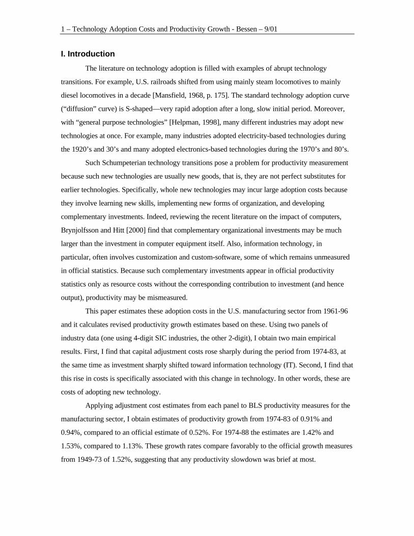
computer. Figure 1 charts the real share of IT investment in total investment; this surged in the late

90’s. The chart also shows the share of nominal investment spent on IT hardware. This rose

sharply from 1974 to 1983 but has remained more or less flat since then. Now although the cost of

computing power has dropped sharply since the mid-80’s, the cost of personal computers has

fallen only slightly [Berndt and Rappaport, 2000]. This means, roughly, that the number of

computers purchased relative to total investment has not changed much since the mid-80’s. Hence

this surge in computing power might not increase adoption costs.

Furthermore, part of the surge in the late 90’s consists of greater software spending. But

this might well be associated with reduced adoption costs. Better software is “user-friendly” and

easier to learn. Also, some portion of adoption costs consists of customization and programming

performed by non-programmers.2 Greater software spending may represent a partial substitution of

purchased software for this activity.

2 The contribution of programming personnel is captured as software in the most recent official statistics [Parker and Grimm,2000], but the activity of non-programmers is not. Historically, few personnel using computers in the early years had computer-specific jobtitles, and today much customization and programming activity is still performed by other occupations, e.g., economists who are SASprogrammers.


More generally, much of this discussion has been framed as an examination of whether the

simultaneous surge in productivity and IT investment represents a “New Economy” or just a

temporary supply shock. The results here suggest a somewhat different picture: we are now well

into the third decade of both strong productivity growth and strong IT investment.

The next section extends the Solow accounting framework to include adjustment costs.

Then in Section III, I use this framework to obtain estimates. Section IV applies these estimates to

the problem of accounting for productivity growth and Section V concludes.

II. Adoption Costs and Technology Transitions

Adjustment Costs

Adjustment costs represent a diversion of output to producing a complement of investment

in capital goods. At time t

(1) ( )ttt cYY −⋅= 1*

where Y is actual output, Y* is potential output, and c is the percentage rate of adjustment costs, a

function of investment. The absolute magnitude of the adjustment cost is *tt Yc ⋅ .

The potential output can be written using a conventional production function

(2) ),,(*ttttt MLKFAY ⋅=

where A represents productivity, K is capital, L is labor and M is materials and energy. I assume

constant returns to scale and competitive markets in L and M. Taking logs, differentiating and

approximating assuming that c << 1 (so that ( ) cc −≈−1ln ),

(3)

tttt

t

t

tt

t

t

t

tt

ttttttttt

M

F

F

M

L

F

F

L

td

cdKMLAY

β−α−=π∂∂

⋅≡β∂∂

⋅≡α

−⋅π+⋅β+⋅α+≈

1,,

ˆˆˆˆˆ

where “^” designates a growth rate and capital is assigned a residual output share. The measured

Solow residual is then (in continuous time)

(4)td

cdAKMLYZ t

ttttttttt −=⋅π−⋅β−⋅α−≡ ˆˆ~ˆ~ˆ~ˆˆ

where α~ and β~

are estimates of the labor and materials elasticities, respectively. In discrete time,


these estimates are usually calculated as the average output share (average of the beginning and

ending period), providing a Tornqvist index of productivity growth.

Equation (4) shows that the Solow residual growth, Z , will be a biased estimator of true

productivity growth if c changes over time. In “normal” circumstances where life proceeds

smoothly along a balanced growth path, c might plausibly change little. However, when firms

make radical shifts in technology, they may incur substantial new costs adopting that technology,

biasing standard productivity measures.

Fortunately, equation (4) provides both a means to estimate c and, with estimates in hand,

a means to adjust productivity measures.

Econometric Specification

Consider first the estimation of adjustment costs. To do this, I assign a functional form to

c. In general, adjustment costs can be described as a function of the investment rate and

technology, ( )TKIcc ,= , where I is investment and T is some measure of technology. I will

defer treatment of T until the next section, leaving just the investment relationship to be specified.

After some experimentation, I chose

(5)1

1

−

−⋅γ=t

tt K

Ic

and several related forms. Then in discrete time, for the ith industry at time t (4) becomes

(6) itti

tiitit K

IaZ ε+

∆⋅γ−µ+=

−

−

1,

1,ˆ

where a represents overall productivity growth captured as a year dummy, µ µ represents an

industry fixed effect, ∆ is the first difference operator and ε ε is a stochastic error term. Note that the

fixed effects capture fixed industry differences in the rate of productivity growth, such as

differences that might arise from differences in R&D spending.

This equation is similar to one used by Lichtenberg [1988] in a study of plant level

adjustment costs. My approach differs from his in several ways. I use a non-parametric measure of

productivity growth as the dependent variable and I scale adjustment costs by the capital stock.

Because I am comparing industries composed of different numbers of plants, it is necessary to

scale investment by some measure of the capital stock. Like Lichtenberg, I use gross rather than


net investment. Lichtenberg, however, does go further and apportions his results between

“replacement” investment and “expansion” investment.

Also, Lichtenberg uses current period investment while I use lagged investment. As

Lichtenberg notes, simultaneity problems bias estimates of γ γ downward when current period

investment is used. By using lagged investment, I avoid this simultaneity issue, although I

potentially understate the total adjustment cost because I miss current period adjustment costs.

On the other hand, if productivity growth is serially correlated and the change in

investment rate is correlated with productivity growth, last year’s simultaneity may also bias my

estimates of γγ. In general these correlations are not large: serial correlation of productivity growth

is -.02 and +.14 for the NBER-CES and BLS samples (described below), respectively. The

corresponding correlations between the change in investment rate and concurrent productivity

growth are .11 and .04. So it is possible that the BLS estimates obtained using (6) may be biased

toward zero. Performing a maximum likelihood AR1 estimation (not shown) generated similar

coefficients and smaller standard errors. For the NBER-CES data, it is possible that some effect

other than adjustment cost might cause the slight negative correlation, overstating estimates of γ.

Tests of Granger causality (not shown) find that changes in the investment rate Granger-cause

productivity growth in both data samples. Thus serial correlation issues do not appear to have

much influence on the estimates obtained using (6).

Note also, that I assign a linear functional form to adjustment costs. This contrasts with

much of the macroeconomic literature that assumes that adjustment costs are convex. My aim (like

Lichtenberg’s) is to assess the magnitude of adjustment cost, not the curvature, so a linear form

should be a reasonable first-order approximation to quadratic forms. In any case, experiments

using quadratic specifications fit the data rather poorly and these specifications were rejected in

favor of linear forms.

The linear specification does not capture fixed costs of adjustment either. However,

episodes of zero investment occur in less than 0.1% of the sample. So fixed costs would be

incurred in virtually all of my data, but the linear specification simply does not capture this effect.

In other words, this specification will understate total adjustment costs if fixed costs occur. Note,

also, that external adjustment costs are not captured.

The (undiscounted) average adjustment cost rate can be calculated using (5) and (1) as


(7)1

**

−

⋅γ=⋅

≡φtK

Y

I

Yc.

This represents the adjustment cost incurred by one dollar of investment. Given the linear

specification, it also equals the marginal adjustment cost.

Measuring Productivity Growth

Equation (4) can be re-arranged

(8)td

cdZA t

tt += ˆˆ ,

indicating that true productivity growth may be obtained by adding dtdc to the measured Solow

residual.

This equation has a straightforward intuitive explanation. The adjustment cost represents a

complementary investment that is not included in measured investment. But this unmeasured

investment is a component of output. That is, Y* is the measure of true output, which is larger than

Y by the amount of investment, *Yc ⋅ . Then, using equation (1), td

cdYY += ˆˆ* , or output grows

faster by dtdc .

I use equation (8) as a simple, basic means to correct measured productivity growth for

adjustment cost changes. This assumes that all other inputs and outputs are measured correctly.

This might not be the case, however, when adoption costs are large. There are two possible,

offsetting effects: adoption costs may distort price deflators for capital goods and adoption costs

may imply unmeasured capital stocks (human and/or physical capital).

First, adoption costs influence the pricing of capital goods in ways that may not be

captured by price deflators. Consider two vintages of a capital good, }1,0{=v , with efficiencies

of vq , adjustment cost rates vφ , and prices vp . Then if these two models are offered at the same

time, it must be true that the costs of efficiency units are equivalent,

(9)1

11

0

00 )1()1(

q

p

q

p φ+⋅=

φ+⋅, or

1

0

0

1

0

1

1

1

φ+φ+

⋅=q

q

p

p.

Note that relative prices are no longer determined solely by relative efficiencies, but relative

adjustment costs also come into play.


This means that quality adjustments used to construct investment deflators will not

properly capture quality differences in the presence of adjustment costs. This is because both the

“matched model” method of deflator construction and hedonic methods assume that efficiency

prices will be equal for two models sold at the same time, or 1100 qpqp = . The matched model

method compares closely similar models at two points in time and then assumes that other models

sold at the same time have the same efficiency prices. The hedonic method performs a cross-

sectional regression of the prices of different models against their characteristics again assuming

efficiency prices are equal across models at any one time.3 Clearly, in the presence of adjustment

costs that may vary from model to model, this assumption will not be true. In particular, if

01 φ>φ , then investment in model 1 will be understated relative to investment in model 0. Note

that this is a measurement problem with quality-adjusted price deflators and since true q is

unobserved, (9) cannot be used to infer values of φ.

Now, the correction in (8) takes care of this measurement problem for capital goods that

are both produced and consumed within the manufacturing sector—for example, the unmeasured

investment in vintage 1 above equals the associated increase in adjustment costs. However, the

manufacturing sector also produces capital goods that are consumed in other sectors. If quality is

mis-measured, then this portion of output is understated and a further adjustment needs to be made.

If the value of capital goods is understated because of rising adjustment costs, then an additional

positive correction to manufacturing productivity growth is needed.

On the other hand, the existence of unmeasured investment suggests that physical capital

stocks or human capital stocks or both may also be mis-measured. Here much depends on the

assumptions made about the nature of this investment, its depreciation rate, factor shares and

whether the transition to new vintages accelerates obsolescence of old capital. If accelerating

adoption costs make capital stocks grow faster than measured, a negative adjustment would have

to be made to (8).

Thus the two possible measurement issues associated with rising adoption costs have

opposite effects on productivity growth estimates. I experimented with a variety of assumptions

regarding these two measurement issues, and found typically: a.) both effects are substantially

smaller than the direct effect of adjustment costs shown in (8), and, b.) the increased growth in

3 In addition, the adjustment rate will be an omitted independent variable, causing hedonic coefficients to be understated. Ifadjustment costs are correlated with quality, then this bias will be reduced, but the basic measurement problem discussed in the textremains.


output tended to be slightly larger than the increased growth in capital stocks. Nevertheless,

because this approach involves some speculation, in this paper I simply use equation (8) to

calculate productivity growth. The reader should interpret the results as a baseline or starting

point. Further research is necessary to evaluate the significance of possible measurement problems.

Finally, note that the role adjustment costs play above is counterpart to another well-

recognized role they play in productivity growth accounting. Adjustment costs are commonly used

to explain the effect of capacity utilization on productivity measurement. Capacity may not be fully

utilized because “quasi-fixed” factors of production, such as capital, adjust only slowly to

economic shocks. Assuming that firms optimize dynamically, a firm faced with a positive

(negative) demand shock may not invest (disinvest) to the optimal long-run level because

investment incurs adjustment costs.4 But clearly, this can only be part of the story. If the

anticipation of adjustment costs prevents firms from fully adjusting capacity, then when firms

finally do invest, they must incur those adjustment costs. And this affects the measurement of

productivity growth.

III. Empirical Results

Data and Variables

To estimate adjustment costs, I use a comprehensive, detailed panel of manufacturing

industries that provides significant cross-sections and time series: the NBER-CES Manufacturing

Industry Database [Bartelsman and Gray, 1996] from 1958 to 1996, which includes 459 industries

at the 4-digit SIC code level (1987 SIC codes). I exclude asbestos products, SIC 3292, an industry

that essentially disappeared in recent years due to legal restrictions.

I also use a smaller panel derived from the April, 2001 release of the BLS multifactor

productivity database.5 This panel includes 19 2-digit SIC industries (I exclude tobacco), however,

it also includes annual measures of IT investment and stocks, permitting investigation of the

relationship between IT and adoption costs.

The variables used are described in the Appendix. However, two deserve further

discussion. First, I experimented with several different specifications for the adjustment cost. As

4 See Dixit and Pindyck [1994] for an overview. See Berndt and Fuss [1986] for the specifics of correcting for capacityutilization in productivity growth accounting.

5 Thanks to Steve Rosenthal and Bill Gullickson for providing requested data.


noted above, the investment measure needs to be scaled by a measure of industry size and I

experimented with different scaling measures, including real output, total capital stock and

structures stock. I obtained the best fit using investment divided by the stock of structures. This

may occur because structures may be measured with less error than equipment. The results below,

however, are based using investment divided by the total capital stock. The adjustment cost

estimates are slightly lower, but the qualitative picture is quite similar.

Second, the capital stocks in the NBER-CES database were developed from industry level

investment data using a perpetual inventory method.6 The specific methodology was developed at

the Federal Reserve Board [Mohr and Gilbert, 1996] and uses BEA deflators (including the

hedonic deflator for computers), stochastic retirements, and beta decay of service efficiency. These

stocks, like the BLS stocks, do not use the BEA depreciation rates that incorporate obsolescence

along with physical depreciation.

To make sure this assumption was not critical, I developed a corresponding series of

capital stocks using the current BEA methods [Katz and Herman, 1997, Fraumeni, 1997]. The

adjustment cost estimates changed only slightly. I also derived estimates using the BLS data (Table

4 below). BLS estimates of productive capital stock weight detailed asset types differently (the

NBER-CES data effectively only have 2 asset classes). The adjustment cost estimates obtained

from the BLS data at the 2-digit level are reasonably close to the estimates from NBER-CES data

at the 4-digit level.

Overall Measures

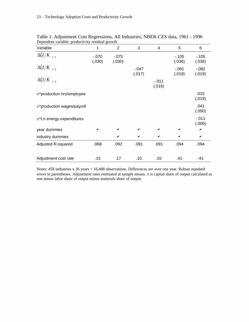
Table 1 presents several variations on equation (6). The first two columns show the

regression with and without industry fixed effects.7 Industry fixed effects control for heterogeneity

in industry-specific factors that might influence the average rate of productivity growth. For

instance, industries with high R&D spending might experience faster productivity growth. If R&D

were also correlated with investment, this might bias the estimates of adjustment costs. As shown

there does not appear to be much bias; fixed effects are used in all subsequent regressions.

Columns 3 and 4 explore different lags in the investment term. The adjustment costs

appear to diminish over time as would be expected. However, investment seems to incur

6 These data only incorporate price deflators for computers from 1972 on. However, computers represent only a tiny fraction ofcapital in 1972, and even less for earlier years, so this should cause no significant bias.

7 Durbin Watson tests do not indicate a problem with serial correlation.


statistically significant costs for up to two years, so I use adjustment terms with both one and two

year lags (Column 5).

Following Berndt and Fuss [1986], I control for capacity utilization effects by assigning

capital a residual share of output in the calculation of the Solow residual. However, this approach

might not fully account for utilization effects if labor or materials do not adjust instantaneously.

Capacity utilization might also effect estimates if returns to scale are not constant. In Column 6, I

also include several measures that may capture capacity utilization. These do not appear to affect

the estimates of adjustment costs.

To estimate the adjustment cost rate, φ, I use sample means and replace potential output

with last year’s actual output, 11 −−⋅γ tt KY . These estimates are shown in the bottom row.

For a single lagged value (Column 2), I find 17¢ of adjustment cost for each dollar of

investment. By comparison, Lichtenberg, using plant level data also derived from the Census of

Manufactures and Annual Survey of Manufactures, finds adjustment costs of 21¢ for replacement

investment and 35¢ for expansion investment. Since the gross investment measure I use is the sum

of replacement investment and expansion investment in Lichtenberg’s study, my estimate based on

industry aggregates is slightly lower than his. However, Lichtenberg uses only a single, current

year of investment.8 When I include investment with a two-year lag, adjustment costs rise to 41¢

per dollar of investment. This is somewhat higher than Lichtenberg’s estimates, however,

considering the differences in method and data, these results are broadly consistent.

Incorrectly measured capital stocks might bias the estimates of adjustment cost. In

particular, if the service efficiency of capital declines more rapidly than accounted for in the

construction of the capital stock, a spurious negative correlation might arise, leading to biased

estimates. Note that the capital stock in the NBER-CES database uses a beta decay model of

service efficiency. This tends to decay less rapidly during the first few years after new capital is

installed. BEA capital stocks, largely based on geometric depreciation, tend to decline more rapidly

than beta decay during the early years of use. To examine the robustness of the estimates, I

constructed a corresponding set of investment rates and capital stocks for each 4-digit industry

using BEA methods and BEA depreciation. Regressions using these alternative stocks did not

generate materially different estimates of adjustment costs (results not shown).

8 Lichtenberg failed to obtain significant results using lagged investment in his specification. However, given the noisiness ofplant level data, this is not surprising.


Time Trends

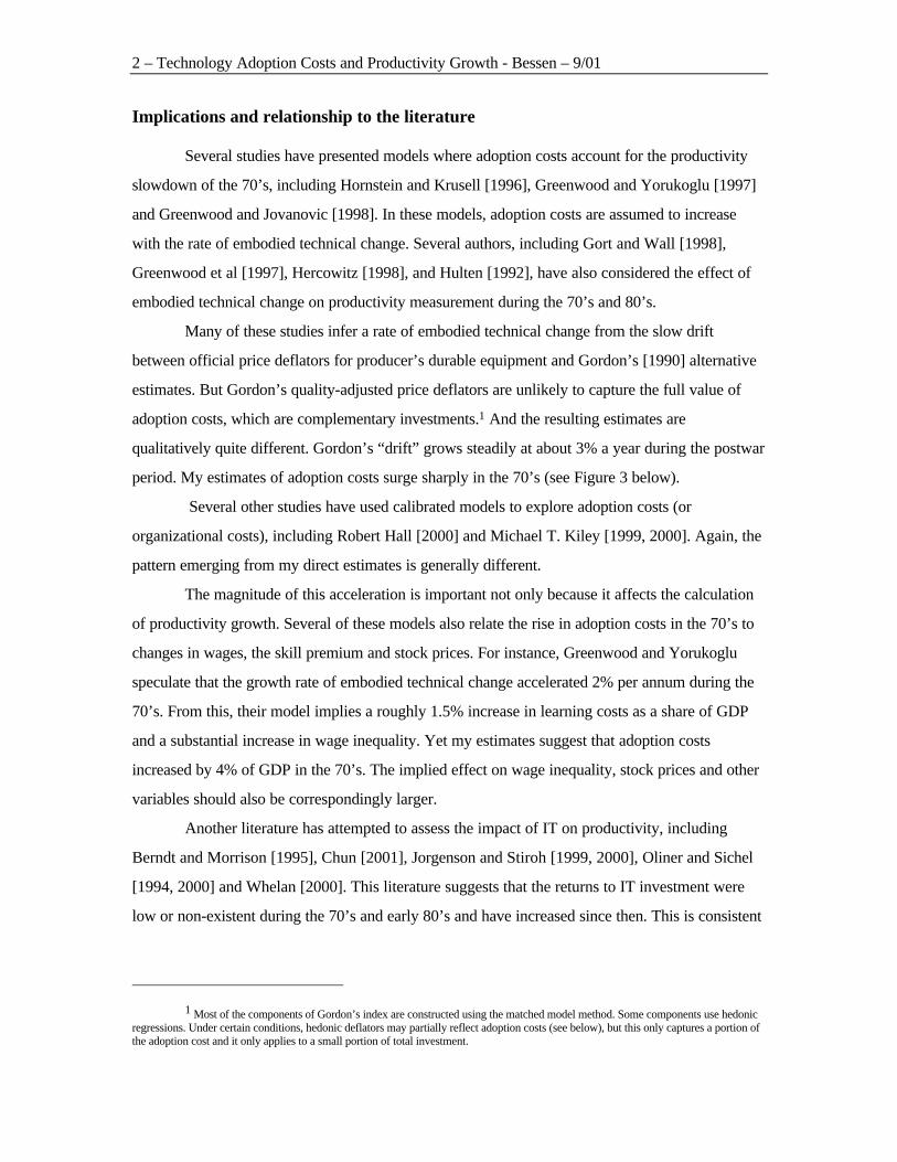
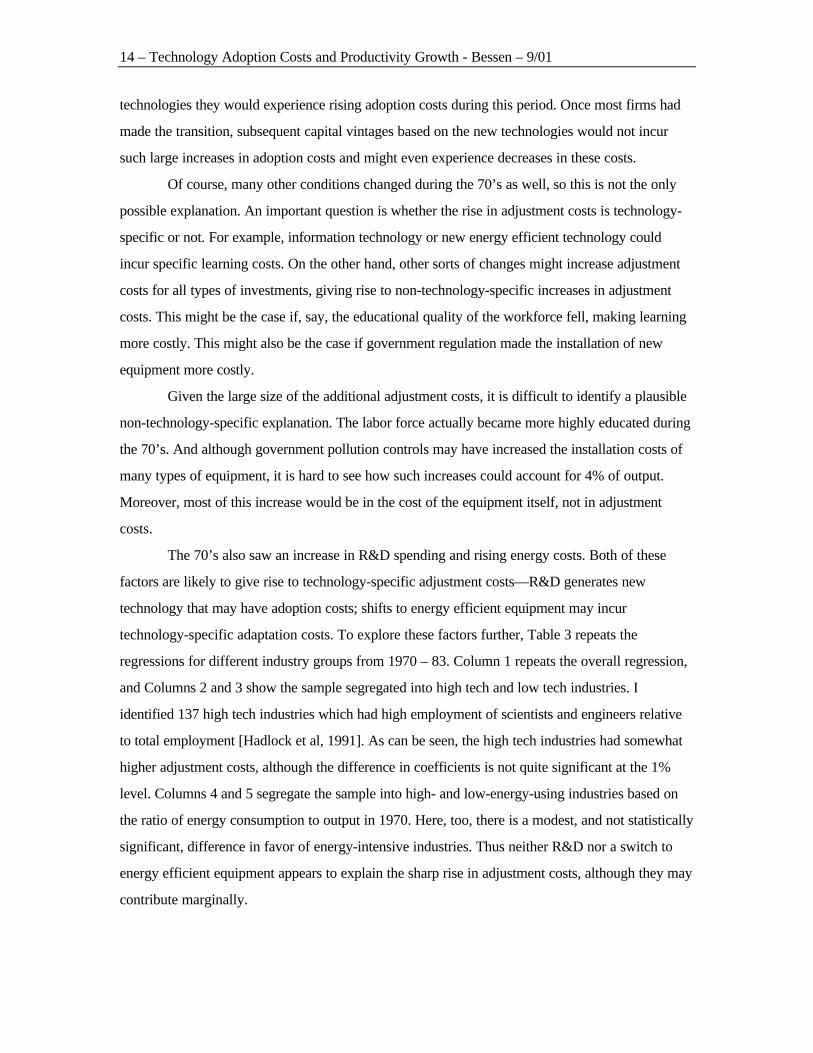
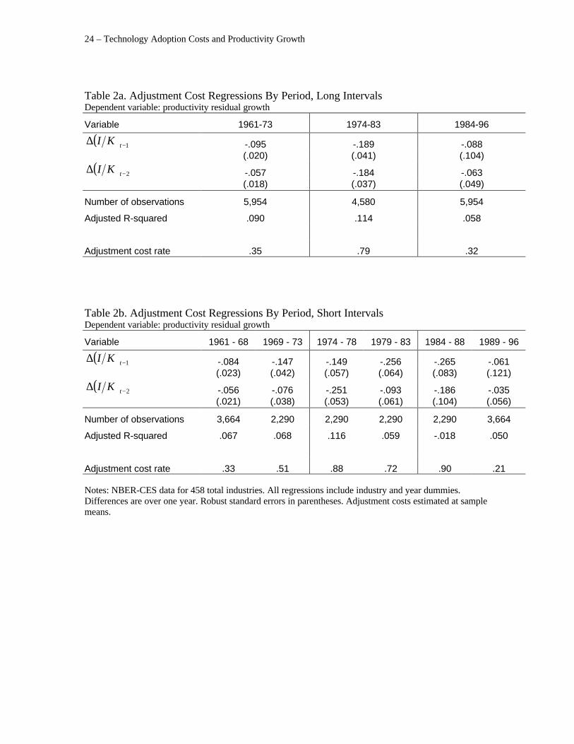
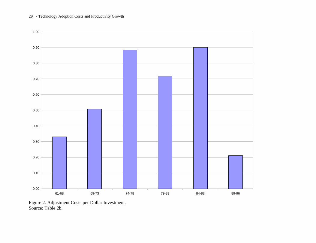
Table 2 presents the regression performed over different intervals. Table 2a shows 3 longer

intervals and Table 2b shows each of these further divided into two shorter intervals. Figure 2

displays the adjustment costs from Table 2b.

A sharp and dramatic pattern emerges. Adjustment costs more than doubled from the early

60’s to the late 70’s and early 80’s. This is a rather large difference. After 1988 the standard errors

grow large and the coefficients lose significance. This change could arise from increased errors in

measuring capital and investment. For instance, the NBER-CES data does not include spending on

unbundled software which looms large in the new BEA and BLS accounts [Parker and Grimm,

2000]. Or it may mean that the new information systems used in different industries have very

disparate effects on adjustment costs.

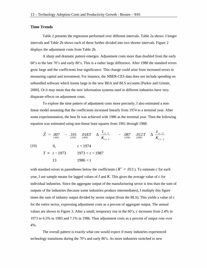
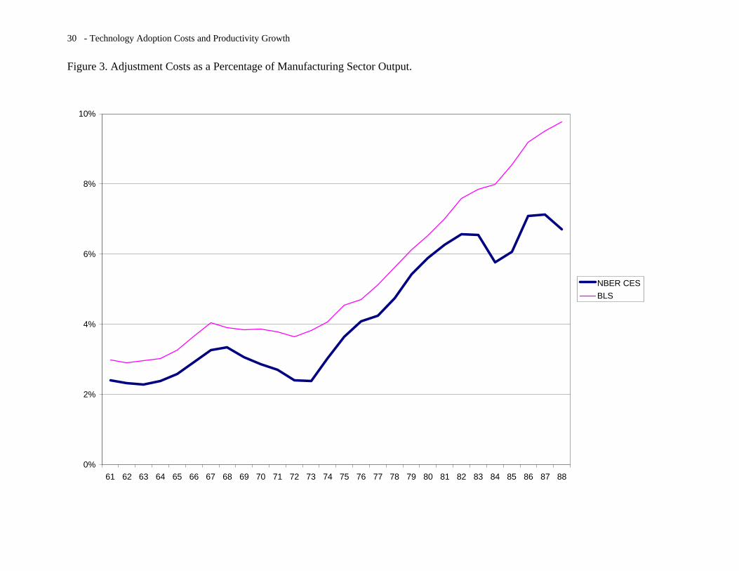
To explore the time pattern of adjustment costs more precisely, I also estimated a non-

linear model assuming that the coefficients increased linearly from 1974 to a terminal year. After

some experimentation, the best fit was achieved with 1986 as the terminal year. Then the following

equation was estimated using non-linear least squares from 1961 through 1988:

(10)

<

<<−

<

≡

∆⋅

+−

∆⋅

+−=

−

−

−

−

t

tt

t

T

K

IT

K

ITZ

ti

ti

ti

ti

198613

198719731973

1974,0

012.087.018.101.007.ˆ2,

2,

)004(.)018(.1,

1,

)004(.)019(.)001(.

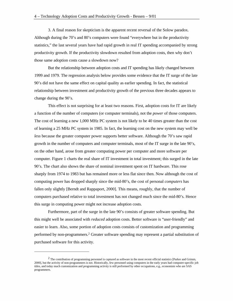
with standard errors in parentheses below the coefficients ( 011.2 =R ). To estimate c for each

year, I use sample means for lagged values of I and K. This gives the average value of c for

individual industries. Since the aggregate output of the manufacturing sector is less than the sum of

outputs of the industries (because some industries produce intermediates), I multiply this figure

times the sum of industry output divided by sector output (from the BLS). This yields a value of c

for the entire sector, expressing adjustment costs as a percent of aggregate output. The annual

values are shown in Figure 3. After a small, temporary rise in the 60’s, c increases from 2.4% in

1973 to 6.5% in 1983 and 7.1% in 1986. Thus adjustment costs as a percent of output rose over

4%.

The overall pattern is exactly what one would expect if many industries experienced

technology transitions during the 70’s and early 80’s. As more industries switched to new


technologies they would experience rising adoption costs during this period. Once most firms had

made the transition, subsequent capital vintages based on the new technologies would not incur

such large increases in adoption costs and might even experience decreases in these costs.

Of course, many other conditions changed during the 70’s as well, so this is not the only

possible explanation. An important question is whether the rise in adjustment costs is technology-

specific or not. For example, information technology or new energy efficient technology could

incur specific learning costs. On the other hand, other sorts of changes might increase adjustment

costs for all types of investments, giving rise to non-technology-specific increases in adjustment

costs. This might be the case if, say, the educational quality of the workforce fell, making learning

more costly. This might also be the case if government regulation made the installation of new

equipment more costly.

Given the large size of the additional adjustment costs, it is difficult to identify a plausible

non-technology-specific explanation. The labor force actually became more highly educated during

the 70’s. And although government pollution controls may have increased the installation costs of

many types of equipment, it is hard to see how such increases could account for 4% of output.

Moreover, most of this increase would be in the cost of the equipment itself, not in adjustment

costs.

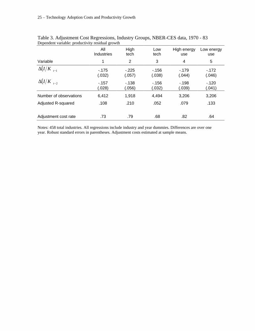
The 70’s also saw an increase in R&D spending and rising energy costs. Both of these

factors are likely to give rise to technology-specific adjustment costs—R&D generates new

technology that may have adoption costs; shifts to energy efficient equipment may incur

technology-specific adaptation costs. To explore these factors further, Table 3 repeats the

regressions for different industry groups from 1970 – 83. Column 1 repeats the overall regression,

and Columns 2 and 3 show the sample segregated into high tech and low tech industries. I

identified 137 high tech industries which had high employment of scientists and engineers relative

to total employment [Hadlock et al, 1991]. As can be seen, the high tech industries had somewhat

higher adjustment costs, although the difference in coefficients is not quite significant at the 1%

level. Columns 4 and 5 segregate the sample into high- and low-energy-using industries based on

the ratio of energy consumption to output in 1970. Here, too, there is a modest, and not statistically

significant, difference in favor of energy-intensive industries. Thus neither R&D nor a switch to

energy efficient equipment appears to explain the sharp rise in adjustment costs, although they may

contribute marginally.


IT and Adjustment Costs

It remains to explore the rise in IT spending as a possible cause of the rise in adjustment

costs. To do this, I use the BLS panel, which includes IT investment.

First, it is necessary to check that this panel has adjustment patterns similar to those in the

NBER-CES data, despite the reduced variation in the cross-sectional dimension. Column 1 of

Table 4 performs a basic adjustment cost regression using a single lagged investment rate. Adding

an additional lag did not generate a significant coefficient. For the single lag, the coefficient is

highly significant and corresponds to an adjustment cost of 57¢ per dollar of investment, somewhat

higher than the 41¢ in Table 1, but reasonably similar given the differences in data and capital

measures.

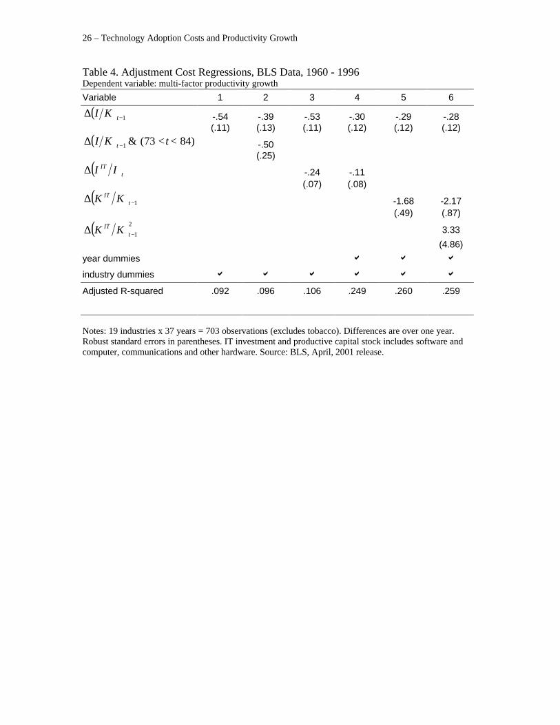
Column 2 tests whether adjustment costs rose sharply in the BLS panel from 1974-83. I

add a variable that is zero outside of this interval and equals the change in the investment rate

during this interval. The coefficient should reflect the increment in adjustment costs during this

period. Although the coefficient is only significant at the 5% level, it is roughly the right magnitude

and reflects a large increase in adjustment costs. Combined, the coefficients imply an adjustment

cost of 94¢ from 1974-83 and of 41¢ before and after this interval. Again, these figures are

somewhat higher than in Table 2a, but reasonably similar. Thus the basic pattern observed in the

much larger NBER-CES database also appears here.

To test for a link between IT spending and adjustment costs, I modify the specification of

adjustment costs in (5) to include a proxy for information technology. The basic intuition is that a

higher share of IT in investment or in the capital stock might incur higher adjustment costs. Two

simple specifications are

(11)t

ITt

t

tt I

I

K

Ic ⋅δ+⋅γ=

−

−

1

1 and1

1

1

1

−

−

−

− ⋅δ+⋅γ=t

ITt

t

tt K

K

K

Ic

where ITI and ITK are real IT investment and stock, respectively. The capital share in second

specification may be thought of as a proxy for relative investment flows over several years. With

these specifications, any increase in IT-intensity incurs a temporary reduction in measured

productivity growth.

Columns 3 and 4 use the first of these specifications, without and with time dummies.

After some experimentation, I found that the regression fit best with zero lag in the IT term, and so

this is what I present in these regressions, despite the possible attenuation of the coefficient because

of simultaneity issues. The IT coefficient is highly significant in Column 3, but when time dummies


are added, the significance disappears. The independent variation in the cross-sectional dimension

of IT investment may simply be insufficient to offset the simultaneity losses.

Column 5 uses the stock specification. This is less volatile and can be used well with a lag.

Here the results with time dummies are highly significant and with a large coefficient for IT share

of capital. Thus there does appear to be a strong link between the IT share and a loss of

productivity.

But does this account for the rise in adjustment costs measured in Table 2? Using (7)

applied to the specification in Column 5 at mean sample values, I calculated the mean adjustment

cost per dollar of investment for the intervals in Table 2a. From 1961-73 the calculated mean

adjustment cost is 37¢, from 1974-83 it is 72¢, and from 1984-96 it is $1.68. Estimates for the

first two intervals match rather closely. Increased IT spending does seem to account for the sharp

increase in adjustment costs in the 70’s and early 80’s. However, after 1984, the estimates diverge.

Recall, however, that the estimates for the last interval in Table 2a have large standard errors and

are not statistically significant, possibly because the NBER-CES data may not fully capture IT

investment. So this divergence is not necessarily at odds with a link between adjustment costs and

IT.

To test whether the linear specification of IT share in Column 5 might cause adjustment

cost estimates in the 90’s to be overstated, I added a quadratic term in Column 6. These estimates

do suggest a slight concavity, but the coefficients are not significant and even then, the estimated

concavity is relatively slight.

Finally, I use the estimates in Column 5 to calculate annual values of c using sample

means. These are also shown in Figure 3 for 1961 through 1988. As can be seen, these estimates

are quite similar to the estimates obtained using NBER-CES detailed industry data, although they

tend to run slightly higher. Thus the two estimates generate a consistent pattern of adjustment

costs, one based on IT and total investment, the other just using investment data.

Based on this evidence, I conclude that the sharp rise in adjustment costs during the 70’s

and early 80’s can be primarily attributed to increased IT investment. Greater R&D and a

transition to energy efficient equipment may have also contributed to a lesser degree. In other

words, adjustment costs rose because of technology adoption costs.


IV. Implications for Productivity Growth Measurement

Adjustments to BLS Estimates for Manufacturing

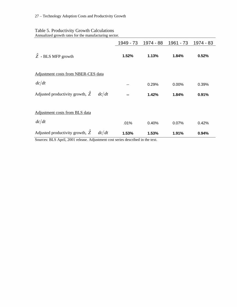
The annual estimates of c displayed in Figure 3 can be used to adjust estimates of

manufacturing sector productivity growth using equation (8). The first row of Table 5 displays the

annualized productivity estimates from the BLS April 2001 release broken into four periods. As

can be seen, these measures exhibit the well-known “productivity slowdown.” Productivity growth

during 1974-88 fell to 1.13% per annum compared to 1.52% during 1949-73.9 Using shorter

intervals, growth fell to 0.52% from 1974-83 compared to 1.84% from 1961-73.

The following two rows show the average annual growth in c and the adjusted productivity

growth estimates using the NBER-CES estimates from (11). The last two rows show comparable

estimates using BLS data with the specification in Column 5 of Table 4. The adjustments have a

substantial impact. A productivity slowdown still appears comparing the shorter intervals, but

comparison of the longer intervals suggests either no slowdown or, at most, a very small

productivity slowdown.

As noted above, these productivity growth estimates ignore possible measurement

problems associated with adoption costs. Nevertheless, these results demonstrate that adoption

costs during technology transitions can easily introduce very large errors into standard productivity

calculations. And the interpretation of technical change during the 70’s lies in the balance.

V. Conclusion

Moses Abramowitz [1956] called the Solow residual a “some sort of measure of

ignorance.” It is, perhaps, comforting to assume that our ignorance grows only gradually and that

the rate of technological change remains more or less constant. But evidence from history and

evidence on the “diffusion” of innovations suggest that technologies frequently exhibit dramatic,

Schumpeterian transitions.

This paper finds evidence of just such a transition during the 1970’s: the cost of installing

and implementing new capital more than doubled. And I find evidence linking this increase to a

greater share of investment in IT. Such a dramatic change suggests that firms experienced large

adoption costs when switching to new technologies. This concurs with case study evidence.

9 A business cycle trough (NBER) occurred during 1949 and a peak in 1973. In 1974 the economy was in recession, but theofficial trough was reached in 1975.


But a rapid increase in adoption costs implies that the Solow residual does not accurately

measure productivity growth. Calculations based on estimated adoption costs demonstrate that

productivity growth may have substantially exceeded the Solow residual during the 70’s, shrinking

the measure of the productivity slowdown. In other words, much of the apparent productivity

slowdown may be an artifact of measurement error. Our ignorance may, in fact, increase sharply

during periods of technological transition.

This is important because, from a longer historical perspective, technology transitions may

not be infrequent. The shift to an increasing share of investment going to information technology is,

in fact, part of a longer secular trend—the share of investment going to equipment has increased

overall (with occasional interruptions) since the nineteenth century. Some of this increase can be

readily identified with new technologies, e.g., the growth in spending on electrical devices and

electric transmission equipment during the middle of the last century.

From this perspective, the 60’s—when measured productivity was high, but also when the

equipment share of investment did not increase—may have been a temporary respite from the

technology transitions implied by this trend. Rather than a “normal” period, this era may have

benefited from improvements to existing technologies without the costs of adopting many new

technologies.

The rise in adoption costs during a technology transition affects more than productivity

growth. Other researchers have argued that adoption costs may also relate to changes in wage

inequality, wage skill premia, the relative employment of skilled workers, and stock prices

[Hornstein and Krusell, 1996, Greenwood and Yorukoglu, 1997, and Greenwood and Jovanovic,

1998]. The results here emphasize the importance of these connections.


Appendix.

Definitions of Variables used in the NBER-CES Estimations

L Labor calculated as annual production hours times the ratio oftotal payroll to production wages. This includes non-production labor in efficiency units.

M Deflated materials and energy.

K Real net capital stock based on FRB methods. Stocks ofindividual asset types are calculated using stochastic servicelives and beta decay of efficiency. Depreciation does notinclude obsolescence. Stocks of different asset types are addedone-for-one to compose aggregate stock.

Y Real output calculated as deflated shipments plus inventorychange.

I / K Investment rate calculated as deflated gross investment dividedby net real plant.

α Labor share of output calculated as total payroll divided bynominal shipments plus inventory change. This quantity isthen multiplied by the ratio of employee compensation towages and salaries found in the NIPA tables for thecorresponding 2-digit SIC industry and year.

β Materials share calculated as nominal cost of materials andenergy divided by nominal shipments plus inventory change.

π Capital share of output calculated as 1 - α - β (assumesconstant returns to scale)

References

Abramovitz, Moses. 1956. “Resource and Output Trends in the United States Since 1870,”

American Economic Review, v. 46, p. 5-23.

Bartelsman, Eric J. and Wayne Gray. 1996. “The NBER Manufacturing Productivity Database,”

NBER Technical Working Paper, No. 205.

Berndt, Ernst and Melvyn Fuss. 1986. “Productivity Measurement with Adjustments for

Variations in Capacity Utilization and Other Forms of Temporary Equilibrium,” Journal

of Econometrics 33, p. 7 – 29.


Berndt, Ernst R. and Catherine J. Morrison. 1995. “High-Tech Capital Formation and Economic

Performance in U.S. Manufacturing Industries: An Exploratory Analysis,” Journal of

Econometrics, v. 65(1), p. 9-43.

Bessen, James. 2000. “Real Options and the Adoption of New Technology.” Research on

Innovation Working Paper.

Black, Sandra E. and Lisa M. Lynch. 2001. “What's Driving the New Economy? The Benefits of

Workplace Innovation,” Federal Reserve Bank of New York Staff Report, No. 118.

Brynjolfsson, Erik and Lorin M. Hitt. 2000. “Beyond Computation: Information Technology,

Organizational Transformation and Business Performance,” Journal of Economic

Perspectives, v. 14, p. 23-48.

Bureau of Labor Statistics. 1997. BLS Handbook of Methods. Washington, DC : U.S. Dept. of

Labor, Bureau of Labor Statistics.

Chun, Hyunbae. 2001. “Can Information Technology Explain Deceleration and Acceleration in

Productivity Growth?,” Working paper.

Comin, Diego. 2000. “An Uncertainty-driven Theory of the Productivity Slowdown:

Manufacturing,” Working paper.

Denison, Edward F. 1989. Estimates of Productivity Change by Industry. Washington, D.C.:

Brookings.

Dixit, Avinash, and Robert Pindyck. 1994. Investment Under Uncertainty, Princeton: Princeton

University Press.

Domar, Evsey D. 1963. “Total Factor Productivity and the Quality of Capital,” Journal of

Political Economy 71, p. 586 – 588.

Eldridge, Lucy P. 1999. “How price indexes affect BLS productivity measures,” Monthly Labor

Review, p. 35-46.

Fisher, Franklin M. 1965. “Embodied Technical Change and the Existence of an Aggregate Capital

Stock,” Review of Economic Studies 32, p. 263 – 88.

Fraumeni, Barbara M. 1997. “The Measurement of Depreciation in the U.S. National Income and

Product Accounts,” Survey of Current Business 77, p. 7 – 23.

Gordon, Robert J. 1990. The Measurement of Durable Goods Prices, Chicago: University of

Chicago Press for the National Bureau of Economic Research.

Gordon, Robert J. 2000. “Does the ‘New Economy’ Measure up to the Great Inventions of the

Past?,” NBER Working Paper 7833.


Gort, Michael and Richard A. Wall. 1998. “Obsolescence, input augmentation and growth

accounting,” European Economic Review 42, p. 1653 – 1665.

Greenwood, Jeremy, Zvi Hercowitz and Per Krusell. 1997. “Long-Run Implications of Investment-

Specific Technological Change,” American Economic Review 87, p. 342 – 362.

Greenwood, Jeremy and Boyan Jovanovic. 1998. “Accounting for Growth,” in C. Hulten, ed.,

Studies in Income and Wealth: New Directions in Productivity Analysis. Chicago:

University of Chicago Press for NBER.

Greenwood, Jeremy and Mehmet Yorukoglu. 1997. “1974,” Carnegie-Rochester Conference

Series on Public Policy, v. 46, p. 49-95.

Hadlock, Paul, Daniel Hecker and Joseph Gannon. 1991. “High technology employment: another

view,” Monthly Labor Review 11, p. 26 – 30.

Hall, Robert E. 2000. “e-Capital: The Link between the Stock Market and the Labor Market in the

1990s.” Unpublished working paper.

Hall, Robert E. and Dale W. Jorgenson. 1967. “Tax Policy and Investment Behavior,” American

Economic Review v 57, p. 391 – 414.

Helpman, Elhanan, ed. 1998. General Purpose Technologies and Economic Growth. Cambridge,

Massachusetts: MIT Press.

Hercowitz, Zvi. 1998. “The ‘embodiment’ controversy: A review essay.” Journal of Monetary

Economics 41, p. 217 – 224.

Hornstein, Andreas and Per Krusell. 1996. “Can Technology Improvements Cause Productivity

Slowdowns?,” in B. Bernanke and J. Rotemberg, eds., NBER Macroeconomics Annual,

1996. Cambridge, Massachusetts: MIT Press.

Hulten, Charles R. 1992. “Growth Accounting When Technical Change is Embodied in Capital,”

American Economic Review v 82, p. 964 – 980.

Hulten, Charles R. 1996. “Quality Change in Capital Goods and its Impact on Economic Growth,”

NBER Working Paper no. 5569.

Jorgenson, Dale W. 1966. “The Embodiment Hypothesis,” Journal of Political Economy 74, p. 1

– 17.

Jorgenson, Dale W. and Kevin Stiroh. 1999. “Information Technology and Growth,” American

Economic Review, Papers and Proceedings, v. 89, p. 109-15.

Jorgenson, Dale W. and Kevin Stiroh. 2000. “Raising the Speed Limit: U.S. Economic Growth in

the Information Age,” Brookings Papers on Economic Activity, 1:2000, p. 125-235.


Katz, Arnold J. and Shelby W. Herman. 1997. “Improved Estimates of Fixed Reproducible

Tangible Wealth, 1929–95,” Survey of Current Business 77, p. 69 – 92.

Kiley, Michael T. 1999. “Computers and Growth with Costs of Adjustment: Will the Future Look

Like the Past?,” Board of Governors of the Federal Reserve System.

Kiley, Michael T. 2000. “Computers and Growth with Frictions: Aggregate and Disaggregate

Evidence,” Board of Governors of the Federal Reserve System.

Lichtenberg, Frank R. 1988. “Estimation of the Internal Adjustment Costs Model Using

Longitudinal Establishment Data,” Review of Economics and Statistics 70, p. 421 – 430.

Lucas, Robert. 1967. “Optimal investment policy and the flexible accelerator,” International

Economic Review, v. 8, p. 78.

Mansfield, Edwin. 1968. Industrial research and technological innovation; an econometric

analysis. New York: Norton.

Mohr, Michael F. and Charles E. Gilbert. 1996. “Capital Stock Estimates for Manufacturing

Industries: Methods and Data,” Board of Governors of the Federal Reserve System.

Mortenson, Dale. 1973. “Generalized costs of adjustment and dynamic factor demand theory,”

Econometrica, v. 97, p. 453.

Oliner, Stephen D. and Daniel E. Sichel. 1994. “Computers and Output Growth Revisited: How

Big is the Puzzle?” Brookings Papers on Economic Activity: Microeconomics, 2 p. 273-

334.

Oliner, Stephen D. and Daniel E. Sichel. 2000. “The Resurgence of Growth in the Late 1990s: Is

Information Technology the Story?” Journal of Economic Perspectives, 14 p. 3-22.

Parker, Robert and Bruce Grimm. 2000. “Recognition of Business and Government Expenditures

for Software as Investment: Methodology and Quantitative Impacts, 1959-98,” Bureau of

Economic Analysis.

Solow, Robert. 1960. “Investment and Technical Progress,” in K. Arrow, S. Karlin and P. Suppes,

eds., Mathematical Methods in the Social Sciences, Stanford: Stanford University Press.

Treadway, Arthur. 1971. “The rational multivariate flexible accelerator,” Econometrica, 39, p.

845.

Whelan, Karl. 2000. “Computers, Obsolescence, and Productivity,” Finance and Economics

Discussion Series No. 2000-6, Federal Reserve Board.

23 – Technology Adoption Costs and Productivity Growth

Table 1. Adjustment Cost Regressions, All Industries, NBER-CES data, 1961 - 1996Dependent variable: productivity residual growth

Variable 1 2 3 4 5 6

( ) 1−∆ tKI -.070 -.075 -.105 -.105(.030) (.030) (.036) (.036)

( ) 2−∆ tKI -.047 -.081 -.082(.017) (.019) (.019)

( ) 3−∆ tKI -.011(.016)

π∗production hrs/employee .015(.019)

π∗production wages/payroll .041(.050)

π∗Ln energy expenditures -.011(.006)

year dummies a a a a a a

industry dummies a a a a a

Adjusted R-squared .068 .092 .091 .091 .094 .094

Adjustment cost rate .15 .17 .10 .02 .41 .41

Notes: 458 industries x 36 years = 16,488 observations. Differences are over one year. Robust standarderrors in parentheses. Adjustment rates estimated at sample means. π is capital share of output calculated asone minus labor share of output minus materials share of output.


Table 2a. Adjustment Cost Regressions By Period, Long IntervalsDependent variable: productivity residual growth

Variable 1961-73 1974-83 1984-96

( ) 1−∆ tKI -.095 -.189 -.088(.020) (.041) (.104)

( ) 2−∆ tKI -.057 -.184 -.063(.018) (.037) (.049)

Number of observations 5,954 4,580 5,954

Adjusted R-squared .090 .114 .058

Adjustment cost rate .35 .79 .32

Table 2b. Adjustment Cost Regressions By Period, Short IntervalsDependent variable: productivity residual growth

Variable 1961 - 68 1969 - 73 1974 - 78 1979 - 83 1984 - 88 1989 - 96

( ) 1−∆ tKI -.084 -.147 -.149 -.256 -.265 -.061(.023) (.042) (.057) (.064) (.083) (.121)

( ) 2−∆ tKI -.056 -.076 -.251 -.093 -.186 -.035(.021) (.038) (.053) (.061) (.104) (.056)

Number of observations 3,664 2,290 2,290 2,290 2,290 3,664

Adjusted R-squared .067 .068 .116 .059 -.018 .050

Adjustment cost rate .33 .51 .88 .72 .90 .21

Notes: NBER-CES data for 458 total industries. All regressions include industry and year dummies.Differences are over one year. Robust standard errors in parentheses. Adjustment costs estimated at samplemeans.


Table 3. Adjustment Cost Regressions, Industry Groups, NBER-CES data, 1970 - 83Dependent variable: productivity residual growth

AllIndustries

Hightech

Lowtech

High energyuse

Low energyuse

Variable 1 2 3 4 5

( ) 1−∆ tKI -.175 -.225 -.156 -.179 -.172(.032) (.057) (.038) (.044) (.046)

( ) 2−∆ tKI -.157 -.138 -.156 -.198 -.120(.028) (.056) (.032) (.039) (.041)

Number of observations 6,412 1,918 4,494 3,206 3,206

Adjusted R-squared .108 .210 .052 .079 .133

Adjustment cost rate .73 .79 .68 .82 .64

Notes: 458 total industries. All regressions include industry and year dummies. Differences are over oneyear. Robust standard errors in parentheses. Adjustment costs estimated at sample means.


Table 4. Adjustment Cost Regressions, BLS Data, 1960 - 1996Dependent variable: multi-factor productivity growth

Variable 1 2 3 4 5 6

( ) 1−∆ tKI -.54 -.39 -.53 -.30 -.29 -.28(.11) (.13) (.11) (.12) (.12) (.12)

( ) )8473(&1 <<∆ − tKI t -.50(.25)

( )tIT II∆ -.24 -.11

(.07) (.08)

( ) 1−∆ tIT KK -1.68 -2.17

(.49) (.87)

( )2

1−∆ tIT KK 3.33

(4.86)

year dummies a a a

industry dummies a a a a a a

Adjusted R-squared .092 .096 .106 .249 .260 .259

Notes: 19 industries x 37 years = 703 observations (excludes tobacco). Differences are over one year.Robust standard errors in parentheses. IT investment and productive capital stock includes software andcomputer, communications and other hardware. Source: BLS, April, 2001 release.


Table 5. Productivity Growth CalculationsAnnualized growth rates for the manufacturing sector.

1949 - 73 1974 - 88 1961 - 73 1974 - 83

Z - BLS MFP growth 1.52% 1.13% 1.84% 0.52%

Adjustment costs from NBER-CES data

dtdc -- 0.29% 0.00% 0.39%

Adjusted productivity growth, dtdcZ +ˆ -- 1.42% 1.84% 0.91%

Adjustment costs from BLS data

dtdc .01% 0.40% 0.07% 0.42%

Adjusted productivity growth, dtdcZ +ˆ 1.53% 1.53% 1.91% 0.94%

Sources: BLS April, 2001 release. Adjustment cost series described in the text.

- Technology Adoption Costs and Productivity Growth28

0 %

5 %

1 0 %

1 5 %

2 0 %

2 5 %

3 0 %

3 5 %

4 0 %

4 5 %

4 8 5 3 5 8 6 3 6 8 7 3 7 8 8 3 8 8 9 3 9 8

R e a l I T ( h d w + s w )

N o m i n a l h a r d w a r e

Figure 1. Share of Manufacturing Investment going to IT.

Source: BLS, April, 2001 Manufacturing and 2-Digit Multifactor Productivity DataTotal IT includes hardware and software; hardware includes computer equipment, communications and other equipment.


0.00

0.10

0.20

0.30

0.40

0.50

0.60

0.70

0.80

0.90

1.00

61-68 69-73 74-78 79-83 84-88 89-96

Figure 2. Adjustment Costs per Dollar Investment.Source: Table 2b.


Figure 3. Adjustment Costs as a Percentage of Manufacturing Sector Output.

0%

2%

4%

6%

8%

10%

61 62 63 64 65 66 67 68 69 70 71 72 73 74 75 76 77 78 79 80 81 82 83 84 85 86 87 88

NBER CES

BLS

Technology Adoption Costs and Productivity Growth: …researchoninnovation.org/qadopt.pdf · 1 –...

Documents

Transcript of Technology Adoption Costs and Productivity Growth: …researchoninnovation.org/qadopt.pdf · 1 –...