Technical Report: Inference of Principal Road Paths Using GPS

Data

Gabriel Agamennoni, Juan I. Nieto and Eduardo M. Nebot

June 4, 2010

Abstract

Over the last few years, electronic vehicle guid-ance systems have become increasingly more pop-ular. However, despite their ubiquity, performancewill always be subject to the availability of detaileddigital road maps. Most current digital maps arestill inadequate for advanced applications in un-structured environments. Lack of up-to-date in-formation and insufficient refinement of the roadgeometry are among the most important shortcom-ings. The massive use of inexpensive GPS receivers,combined with the rapidly increasing availabilityof wireless communication infrastructure, suggeststhat large amounts of data combining both modal-ities will be available in a near future. The ap-proach presented here draws on machine learningtechniques and processes logs of position traces toconsistently build a detailed and fine-grained rep-resentation of the road network by extracting theprincipal paths followed by the vehicles. Althoughthis work addresses the road building problem invery dynamic environments such as open-pit mines,it is also applicable to urban environments. Newcontributions include a fully unsupervised segmen-tation method for sampling roads and inferring thenetwork topology, a general technique for extract-ing detailed information about road splits, mergesand intersections, and a robust algorithm that ar-ticulates these two. Experimental results with datafrom large mining operations are presented to vali-date the new algorithm.

Digital road maps, data mining, machine learn-ing, GPS, road safety.

1 Introduction

In the last few years, the wide availability of com-mercial digital road maps has enabled a large num-ber of vehicle navigation and guidance applications.Commercial vector maps have managed to cover toa great extent the major road networks in urbanareas, achieving a level of accuracy in the order of

a few to a few tens of meters. The combination ofthese digital maps with precise positioning systemshas allowed the development of numerous in-vehicleapplications that provide navigation aid and driv-ing assistance. However, there exists a much widerrange of potential applications beyond those aimedat enhancing driver convenience. As shown in [1],detailed road maps could also be used to improveroad safety by means of lane keeping, rollover warn-ing, obstacle detection and collision avoidance sys-tems.

A fundamental limitation of commercially avail-able road maps is their lack of fine-grained informa-tion. Standard high-end road safety applicationsrequire not only accuracy but also a superior levelof detail, and currently this can only be achievedby the use of probe vehicles and manual surveyingmethods. The resulting map is therefore very ex-pensive and time-consuming to build and update.Many authors [2, 3, 4, 5] propose that, instead ofusing a single dedicated probe to generate such anenhanced map, a large number of inexpensive low-precision information sources could yield similar oreven better results. With the emergence of low-cost positioning devices and the accelerated devel-opment of wireless communication systems, inte-grated data gathering and processing becomes fea-sible at a very large scale. This allows large volumesof position data to be recorded and used for learningor updating the road map. Even though the datais polluted with noise and outliers, its abundancecompensates for its lower quality. The resultingroad map is not only more precise and more re-fined, but can also be updated continuously as newinformation becomes available.

An important distinction is to be made betweenthe usual notion of a road map and the enhancedmaps which are the focus of this article. Commer-cially available GPS devices usually contain a digi-tal map which they use for localization and for pro-viding directions to the user. These are fairly com-monplace and readily available from web resourcesand GPS manufacturers. However, their lack of de-tail renders them ineffective for road safety applica-

1

tions. In contrast, the class of refined maps that arethe focus of the present work do have a lot potentialwhen it comes to safety. These enhanced maps aremuch richer in detail and contain far more infor-mation. They not only describe the road geometryand the network topology but also contain statis-tics about the way agents move. They character-ize the “normal” or “standard” behavior of vehiclesand capture typical vehicle paths as they traversethe circuit. Their additional information contentmakes them particularly valuable when assessingsafety. For example, abnormal behavior can be de-tected by comparing an agent’s movement patternwith the map’s statistics.

In order to distinguish between the two classesof maps, the term Principal Road Path map is in-troduced here. Principal road path map, or PRPmap, will be used hereafter to refer to the classof enhanced maps previously described. The nameemphasizes the importance of typical driving be-havior in road safety applications. Its meaning aswell as its motivation will be explained in more de-tail in the following sections.

1.1 Principal road paths and roadsafety

PRP maps enable numerous road safety applica-tions. For instance, an adaptive cruise control sys-tem could operate basing its decisions on curvatureand elevation in order to minimize rollover risk.Also, a high degree of map detail would enable pre-cise lane-level tracking for a lane departure warningmechanism and even fault detection for inferringobstructed sections in a road. Several degrees ofdriver interaction are possible, ranging from unob-trusive driving assistance to full automatic control.Also, wireless communication systems could allowinformation to be shared across multiple nearbyagents. This would enable vehicles to incorporatecontext-aware systems, and eventually to developcooperative decision-making schemes.

An important area of application of PRP mapsis mining safety. Every year there are a large num-ber of accidents involving collisions between haultrucks and other mine resources such as light vehi-cles, graders and loaders. Many of them result infatalities and significant loss of equipment and pro-duction. There are many causes behind these acci-dents, the most important one being operator’s lackof situational awareness [6]. Open-pit mines arevery dynamic and hostile environments. Drilling,Loading and stockpiling areas are constantly chang-ing due to the progress of the mine process, andhaul roads are continuously modified accordingly.Visibility is extremely limited by the size of the ma-

chinery and the configuration of the cabin, whichcreates large blind spots in the driver’s field of view.Furthermore, it is often severely impaired by harshenvironmental conditions such as fog, dust, rainand snow. This poses a great safety hazard, es-pecially in difficult areas such as intersections withtall banks and and roads with different grades.

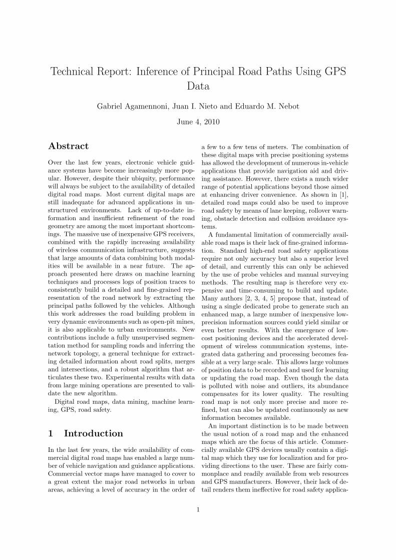
Figure 1 shows a snapshot of a typical large-scalemine with many haul roads, intersections, loadingand drilling areas. During the course of operationof the mine, heavy machinery such as haul trucks,graders, drills and shovels are closely interactingwith light vehicles. The location marked as “A” isa loading area. Here, the haul trucks queue as theywait to be loaded with ore by the shovel. Location“B” is an intersection where two roads with differ-ing grades converge. Both roads are bounded oneach side by a berm, which is taller than the lightvehicles, meant to prevent haul trucks from veeringoff the edge1. Immediately below this intersection,the road is being widened to provide access to thedrilling area. Once drilling has finished, the areawill turn into another loading site similar to “A”.As this figure shows, the opencast mine scenariocan be very complex and dynamic.

Figure 1: Snapshot of the operation of a large open-cast mine. Loading and drilling areas are markedwith letters. See text for details.

Previous work has shown the importance of sit-uational awareness in mining safety [7, 8, 6]. Therehas been significant progress in this area, with thedeployment of systems that provide peer-to-peer

1Notice the size of the light vehicles with respect to thetrucks. A standard 4WD is less than 4 meters long and 2meters high, whereas a haul truck is typically more thanthree times as large. In fact, the blind spot at the front of ahaul truck can be large enough to shadow a 4WD completely.

2

communication between resources to make themaware of vehicles in their proximity. More recently,the concept of “context” has been introduced toevaluate risk according to the information that iscurrently available, and to generate proper feedbackfor the operator. Generating just the right amountof feedback is essential. Most of the time proximityevents do not represent a threat that warrants analarm. Therefore, a system that is overly conserva-tive would generate a large number of false alarmsand will end up being counterproductive, overbur-dening the driver with useless information.

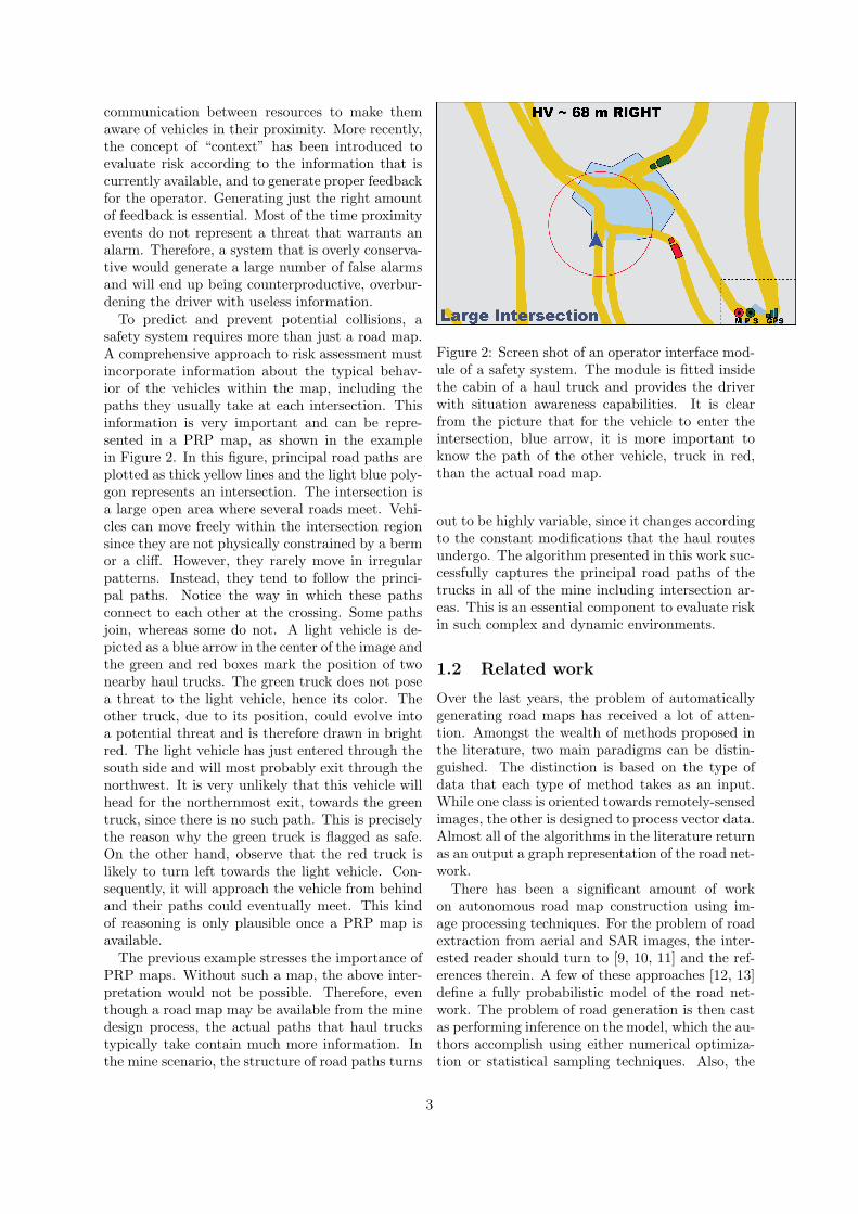
To predict and prevent potential collisions, asafety system requires more than just a road map.A comprehensive approach to risk assessment mustincorporate information about the typical behav-ior of the vehicles within the map, including thepaths they usually take at each intersection. Thisinformation is very important and can be repre-sented in a PRP map, as shown in the examplein Figure 2. In this figure, principal road paths areplotted as thick yellow lines and the light blue poly-gon represents an intersection. The intersection isa large open area where several roads meet. Vehi-cles can move freely within the intersection regionsince they are not physically constrained by a bermor a cliff. However, they rarely move in irregularpatterns. Instead, they tend to follow the princi-pal paths. Notice the way in which these pathsconnect to each other at the crossing. Some pathsjoin, whereas some do not. A light vehicle is de-picted as a blue arrow in the center of the image andthe green and red boxes mark the position of twonearby haul trucks. The green truck does not posea threat to the light vehicle, hence its color. Theother truck, due to its position, could evolve intoa potential threat and is therefore drawn in brightred. The light vehicle has just entered through thesouth side and will most probably exit through thenorthwest. It is very unlikely that this vehicle willhead for the northernmost exit, towards the greentruck, since there is no such path. This is preciselythe reason why the green truck is flagged as safe.On the other hand, observe that the red truck islikely to turn left towards the light vehicle. Con-sequently, it will approach the vehicle from behindand their paths could eventually meet. This kindof reasoning is only plausible once a PRP map isavailable.

The previous example stresses the importance ofPRP maps. Without such a map, the above inter-pretation would not be possible. Therefore, eventhough a road map may be available from the minedesign process, the actual paths that haul truckstypically take contain much more information. Inthe mine scenario, the structure of road paths turns

Figure 2: Screen shot of an operator interface mod-ule of a safety system. The module is fitted insidethe cabin of a haul truck and provides the driverwith situation awareness capabilities. It is clearfrom the picture that for the vehicle to enter theintersection, blue arrow, it is more important toknow the path of the other vehicle, truck in red,than the actual road map.

out to be highly variable, since it changes accordingto the constant modifications that the haul routesundergo. The algorithm presented in this work suc-cessfully captures the principal road paths of thetrucks in all of the mine including intersection ar-eas. This is an essential component to evaluate riskin such complex and dynamic environments.

1.2 Related work

Over the last years, the problem of automaticallygenerating road maps has received a lot of atten-tion. Amongst the wealth of methods proposed inthe literature, two main paradigms can be distin-guished. The distinction is based on the type ofdata that each type of method takes as an input.While one class is oriented towards remotely-sensedimages, the other is designed to process vector data.Almost all of the algorithms in the literature returnas an output a graph representation of the road net-work.

There has been a significant amount of workon autonomous road map construction using im-age processing techniques. For the problem of roadextraction from aerial and SAR images, the inter-ested reader should turn to [9, 10, 11] and the ref-erences therein. A few of these approaches [12, 13]define a fully probabilistic model of the road net-work. The problem of road generation is then castas performing inference on the model, which the au-thors accomplish using either numerical optimiza-tion or statistical sampling techniques. Also, the

3

work in [5] proposes a method where image pro-cessing tools are applied to vector data. After con-structing a two-dimensional histogram from GPSdata logs, the authors recover the skeleton of thenetwork by means of simple linear filtering and mor-phological operations.

Approaches based purely on vector data alsoabound in the literature. Some of these [14, 2] as-sume the existence of an initial base map, consist-ing of a commercially available road map or con-structed from a grey scale image [15]. From thisinitial estimate, the authors progressively refine themap by fusing it with GPS information. Other ap-proaches build the map from the start assuming noprior knowledge. For instance, the authors of [2, 16]draw on the field of computational geometry anduse the sweep-line algorithm to efficiently build atravel graph from vector data. Others [17] con-struct the graph by defining a clustering scheme tolink GPS traces together. The approach introducedin [4] defines a graph-matching technique that is in-cremental and specifically designed for real-time ap-plications. One of the approaches that is most rele-vant to the one presented here is the work of [3]. Inthis case, the strategy consists of placing road seedsand linking them together according to transitioncounts.

This article is organized as follows. Section 2presents the road model utilized throughout therest of the paper. The fundamental components ofthe map building algorithm, Sampling and Linking,are presented in sections 3 and 4 respectively. Re-sults are presented in Section 5 along with a thor-ough discussion and a brief comparison to othermapping algorithms. Section 6 draws conclusionsand discusses future research directions. Finally,Appendix 7 contains a few useful definitions relatedto graph theory, and Appendix 8 and 9 mention im-portant practical considerations for implementingthe algorithm.

2 Road Model

This section explains the road model adoptedthroughout this work. Before explaining the algo-rithm itself, it is necessary to lay the foundationsby setting forth in words the way a road networkis conceived. First, the structure that is chosen forrepresenting the map is described. Then, each ofits constituent elements is explained in turn. Thisdiscussion serves as a starting point for developingthe algorithm in full depth and leads seamlessly intoSection 3, where all the details are given.

2.1 Representing the network

Commercial digital road maps usually consist ofan attributed undirected graph. Junctions or in-tersections are represented as vertices with degree2

greater than two, whereas roads are depicted as asequence of edges. Since the graph is undirected,a path possesses no orientation and hence two-wayroads are considered as a single path. The presentapproach will depart from this convention, adopt-ing the view of [3, 4] instead. Specifically, roads willbe regarded as a sequence of directed edges, essen-tially splitting each bidirectional road into a pair ofunidirectional road paths. Doing so will yield muchbetter discrimination of the dominant directions incluttered areas, as will be shown later on.

Additional attributes can be defined to comple-ment the graph. Geometric features such as widthand curvature can be present as part of the mapdescription. These features are essential for roadsafety applications because they provide detailedinformation about the local geometry. Likewise,label attributes such as “junction” and “bidirec-tional” can also prove useful since they give a qual-itative high-level characterization of the network.There is a wide variety of attributes that can bedefined. Many of these encode important informa-tion regarding the way vehicles move, or are sup-posed to move, as they traverse the network. Theyimpose restrictions on vehicle behavior, and hencecan be extremely valuable for assessing risk. Theend result is a structure that comprises not onlythe skeleton of the roads and their interconnections,but also a rich combination of edge- and vertex-level attributes containing a wealth of fine-grainedinformation.

The core of the map structure lies in its directedgraph. The graph constitutes the skeleton of thenetwork. It also induces a representation of theroad paths. Specifically, a finite sequence of con-nected nodes on the graph can be seen as a se-quence of samples of a particular road path. Theunderlying road path would then be a curve thatinterpolates the nodes on the sequence. Conversely,from a generative point of view, the principal roadpath may be regarded as a hidden generating curvethat maps distances along the road to positions inthree-dimensional space.

It is important to distinguish between the graphitself and its corresponding node set. A node assuch is a real-valued point that marks a physicallocation on the map, whereas a graph is the mathe-matical object that links all the nodes together. Asalready mentioned, direction information becomes

2The degree of a vertex is the number of edges incidenton it.

4

extremely valuable when dealing with cluttered re-gions. For this reason, it is already incorporated aspart of the map representation by directly workingin joint position-velocity space. That is, each nodeis considered as being composed of six real num-bers; the (x, y, z) position triple and the (u, v, w)velocity triple. As a consequence of this construc-tion, all of the nodes, and hence all road traces,not only lie on the principal road path but are alsotangent to it.

2.2 Principal curve

The concept of a principal road path can be de-fined concisely in mathematical terms. Specifically,it can be seen as the principal curve of a set of po-sition data traces. Thus the motivation behind theterm PRP becomes clear. The remainder of thissection is set apart for the purpose of defining theprincipal curve. The intuition behind this conceptand its relationship to the principal road path willbe explained in detail in the next section.

Definition 1. Let I ∈ R be a compact connectedsubset of the real line. A real, d-dimensional para-metric curve c is a continuous mapping c : I 7→c(I) ⊂ Rd. The domain of c is denoted as D(c) = I.

Definition 2. Let Cd be the set of all real, d-dimensional curves. A reparameterization of acurve c ∈ Cd is a bijective mapping r : I 7→ D(c).Notice that, in general, I and D(c) need not beequal.

The following is a definition of a principal curve.It generalizes the one given in [18] to the case wherethe data contains temporal information. In thiscase, instead of a set of points in Euclidean space,the data is taken to be a set of arbitrary curves. Itcan be easily verified that this definition reduces tothe original definition in the limit where all curveshave zero length.

Definition 3. Let p be a probability measure onCd. The curve γ ∈ Cd is a principal curve of p ifit is self-consistent in all of its domain, that is if∀ t ∈ D(γ),

γ (t) = E[c (u)

∣∣r−1c (u) = t

], (1)

where the function rc : I ⊆ D(γ) 7→ D(c) is areparameterization of c ∼ p.

The mapping rc projects the any given curvedrawn from p onto the principal curve. It yieldsa matching of c to γ by associating every point γ(t)with another point c(u), where u = rc(t). Noticethat the domain of rc is constrained to be a sub-set of the domain D(γ) of γ. Because in general it

may be a proper subset of D(γ), the curve match-ing need not be complete. However, rc must be asurjective function and therefore every point on cmust originate from a corresponding point on theprincipal curve.

The reparameterization plays a key role in Defini-tion 3. The self-consistency property in Equation 1states that every point on γ must equal the sta-tistical mean of all points on any given curve thatproject to it. Projection is achieved by applicationof the mapping rc and can be chosen according toan optimality criterion. Namely, it can be chosento minimize a distance functional,

rc = arg minrd (c ◦ r, γ) ,

where d : C × C 7→ R+ ∪ {0} is a distance metric,such as the Frechet distance [19], that measures thedissimilarity between two given curves.

In practice, the distribution p is seldom known.Instead, only a finite data set is available. Each el-ement of the data set usually comprises a sequenceof data points of the same dimension. For example,when reconstructing road maps from vector data,the data set usually consists of a set of positiontraces. After linear interpolation, these traces be-come polygonal line curves. Evaluating the Frechetdistance for polygonal line curves can be done ef-ficiently, as shown in [19], and yields the matchingfunction rc as a byproduct. Therefore, estimatingthe principal curve of the data set could be accom-plished efficiently via a straightforward extensionof the polygonal line algorithm of [20] to curvilin-ear data. However, as will be shown in Section 3,this method is only adequate for the case of a sin-gle isolated road. When multiple roads coexist, themethod is no longer applicable due to the data as-sociation problem that arises.

3 Sampling

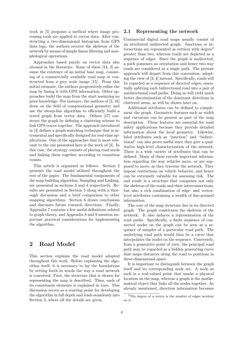
This section and the following one develop the map-building algorithm step by step in two separateparts. Each part is focuses on a particular pro-cessing stage. A basic outline of the two stages ofthe algorithm can be seen in the diagram in Fig-ure 3. First, the road network is sampled at anumber of nodes along the principal road paths.Afterwards, these nodes are incrementally linkedtogether, producing the final graph. The presentsection describes the first stage of the algorithm,called the sampling stage.

5

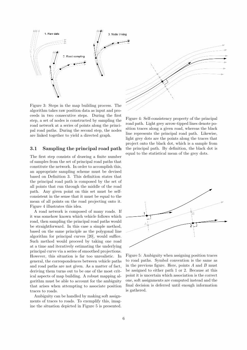
Figure 3: Steps in the map building process. Thealgorithm takes raw position data as input and pro-ceeds in two consecutive steps. During the firststep, a set of nodes is constructed by sampling theroad network at a series of points along the princi-pal road paths. During the second step, the nodesare linked together to yield a directed graph.

3.1 Sampling the principal road path

The first step consists of drawing a finite numberof samples from the set of principal road paths thatconstitute the network. In order to accomplish this,an appropriate sampling scheme must be devisedbased on Definition 3. This definition states thatthe principal road path is composed by the set ofall points that run through the middle of the roadpath. Any given point on this set must be self-consistent in the sense that it must be equal to themean of all points on the road projecting onto it.Figure 4 illustrates this idea.

A road network is composed of many roads. Ifit was somehow known which vehicle follows whichroad, then sampling the principal road paths wouldbe straightforward. In this case a simple method,based on the same principle as the polygonal linealgorithm for principal curves [20], would suffice.Such method would proceed by taking one roadat a time and iteratively estimating the underlyingprincipal curve via a series of smoothed projections.However, this situation is far too unrealistic. Ingeneral, the correspondences between vehicle pathsand road paths are not given. As a matter of fact,deriving them turns out to be one of the most crit-ical aspects of map building. A robust mapping al-gorithm must be able to account for the ambiguitythat arises when attempting to associate positiontraces to roads.

Ambiguity can be handled by making soft assign-ments of traces to roads. To exemplify this, imag-ine the situation depicted in Figure 5 is presented.

Figure 4: Self-consistency property of the principalroad path. Light grey arrow-tipped lines denote po-sition traces along a given road, whereas the blackline represents the principal road path. Likewise,light grey dots are the points along the traces thatproject onto the black dot, which is a sample fromthe principal path. By definition, the black dot isequal to the statistical mean of the grey dots.

Figure 5: Ambiguity when assigning position tracesto road paths. Symbol convention is the same asin the previous figure. Here, points A and B mustbe assigned to either path 1 or 2. Because at thispoint it is uncertain which association is the correctone, soft assignments are computed instead and thefinal decision is deferred until enough informationis gathered.

6

This figure shows a single position trace that mustbe attributed to one of two different road paths.At this stage it is still not clear which assignmentis true one. So, instead of making a hard deci-sion, soft probabilistic assignments are computedand the final judgement is delayed until more ev-idence is collected. Elaborating a model capableof propagating this uncertainty is one of the maincontributions in this article.

3.2 Initial estimate

Suppose for a moment that an estimate is provided.Namely, let xm, ym be a node that approximatesthe principal road path at a given point. Recallthat each individual node comprises both a posi-tion and a direction vector, as discussed previously.Hence the pair (xm,ym) uniquely defines an ori-ented plane πm that passes through xm and is nor-mal to ym. Direction vector ym defines the positiveorientation for this plane.

On the other hand, a set of position data tracesis also given. Each trace is composed of a finitesequence of position samples ordered according totime. Time stamps need not be given explicitly butmust agree with sample indices. That is, they mustbe monotonically increasing in such a way that m <n implies that sample m was taken before samplen. Note that the associated time stamps need notbe uniformly spaced and may contain gaps due tomissing data. In order to ensure a minimum degreeof spatial continuity, data traces containing gapslarger than a few seconds must be split.

The sequence of points on each data trace is in-terpolated by a curve. There are many possiblecriteria for interpolating a sequence of points inEuclidean space, being nearest neighbor the sim-plest one. However, recall from Definition 1 thatcurves must be continuous. This is why linear in-terpolation is chosen instead, since it is the methodthat immediately follows nearest neighbor in termsof complexity. Instant velocity can be estimatedvia numerical differentiation or Kalman filtering.Section 5 will demonstrate that even a very crudeapproximation such as finite differences yields sur-prisingly good results.

Curves and road samples relate in the followingway. Let zn be the curve that interpolates the n-thposition trace in the data set. Let T (m)

n be the setof all parameter values whose corresponding imageunder zn intersect πm with strictly positive orien-tation,

T (m)n =

{t : (zn(t)− xm)Tym = 0,

dzndt

(t)Tym > 0}

(2)

Since each trace contains a limited number ofpoints, and from construction of the trajectories,T

(m)n must be a finite set. Therefore, the union of

all the images under zn and dzn/dt

X(m) =⋃n

zn(T (m)n

)= {x(m)

k },

Y (m) =⋃n

dzndt

(Tn) = {y(m)k }

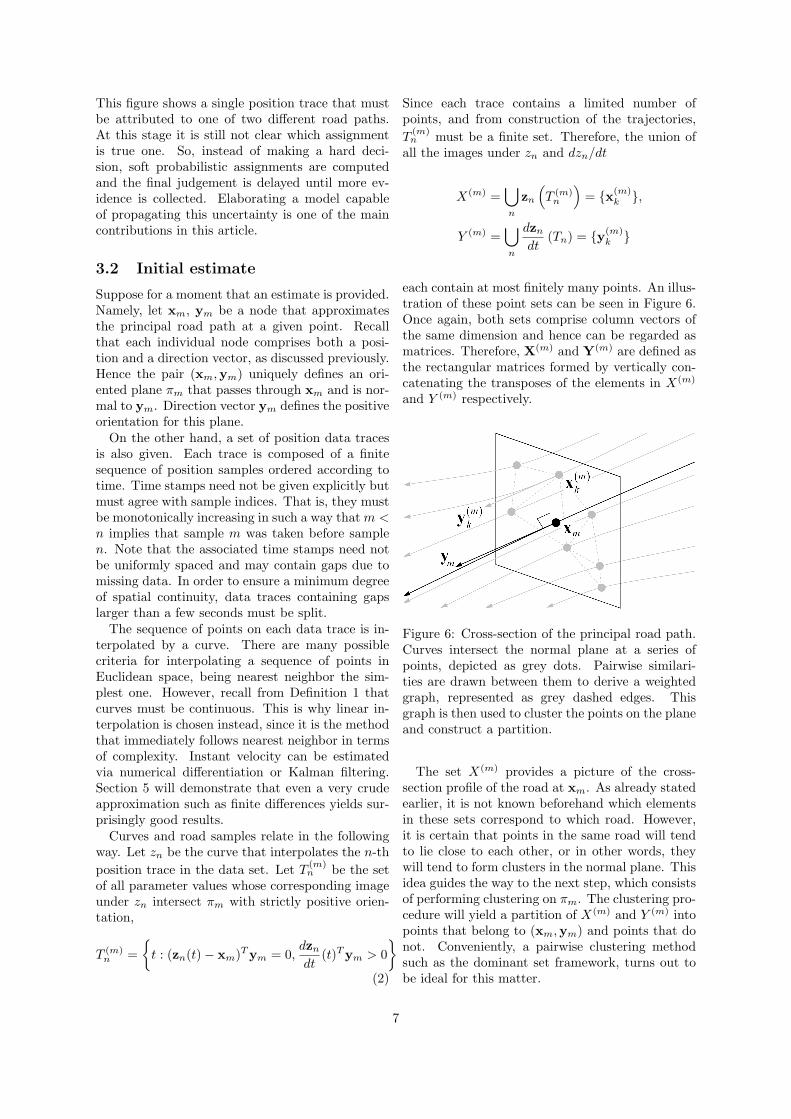
each contain at most finitely many points. An illus-tration of these point sets can be seen in Figure 6.Once again, both sets comprise column vectors ofthe same dimension and hence can be regarded asmatrices. Therefore, X(m) and Y(m) are defined asthe rectangular matrices formed by vertically con-catenating the transposes of the elements in X(m)

and Y (m) respectively.

Figure 6: Cross-section of the principal road path.Curves intersect the normal plane at a series ofpoints, depicted as grey dots. Pairwise similari-ties are drawn between them to derive a weightedgraph, represented as grey dashed edges. Thisgraph is then used to cluster the points on the planeand construct a partition.

The set X(m) provides a picture of the cross-section profile of the road at xm. As already statedearlier, it is not known beforehand which elementsin these sets correspond to which road. However,it is certain that points in the same road will tendto lie close to each other, or in other words, theywill tend to form clusters in the normal plane. Thisidea guides the way to the next step, which consistsof performing clustering on πm. The clustering pro-cedure will yield a partition of X(m) and Y (m) intopoints that belong to (xm,ym) and points that donot. Conveniently, a pairwise clustering methodsuch as the dominant set framework, turns out tobe ideal for this matter.

7

3.3 Clustering on the normal hyper-plane

Clustering by searching for dominant sets on aweighted graph is described in Appendix 8. Thedominant set framework is particularly effective atfinding compact groups of points, and hence it is es-pecially well suited for the purpose of finding princi-pal paths. In order to apply this method, a suitablesimilarity measure must be derived. Thorough ex-perimentation led to the conclusion that distanceand angle are the only two critical factors for clus-tering on the normal hyperplane. Specifically, let

dij = ‖x(m)i − x(m)

j ‖, aij = cos−1y(m)i · y(m)

j

‖y(m)i ‖‖y(m)

j ‖

denote the Euclidean distance between points x(m)i

and x(m)j in X(m), and the angle between their cor-

responding derivative vectors in Y (m), respectively.After thorough experimentation, it was found bytrial and error that the expression

w(i, j) ∝ e−d2ij/ε

2 + κ (1− cos aij) (3)

yields very good results. This similarity functionarises from the product of a Gaussian and a VonMises-Fisher density. Both ε and κ are positivescalars that control the concentration of the distri-bution around its mean.

The reader should take a moment to examineEquation 3. Constants ε and κ are two parame-ters that account for uncertainty in the model. Thefirst one corresponds to the standard deviation ofa Gaussian distribution and has units of distance,while the second corresponds to the angular con-centration parameter of a spherical density functionand is dimensionless. Both parameters quantify thescattering in position and the dispersion in direc-tion. Increasing the value of ε, or decreasing thevalue of κ, equates to admitting a higher noise levelin the data. However, their choice also involves acompromise between accuracy and noise immunity.Too large a value can result in significant errors,whereas a low value can lead to over-segmentation.

In practice, an equivalent and more intuitive pa-rameter is used instead of angular concentration.Namely, the standard deviation δ is a more naturalway of quantifying the degree of spread. For theVon Mises-Fisher distribution there exists a bijec-tion between concentration and standard deviation,both relating via the following equation(

δ

2π

)2

= 1−(

Id/2 (κ)Id/2−1 (κ)

)2

,

where Ij denotes the modified Bessel function oforder j and d is the dimensionality of the data.Therefore, given a value for δ, the correspondingconcentration value for Equation 3 can be deter-mined by numerically solving the equation above.Standard deviation is given in radians and variesfrom 0 to 2π.

Having selected a suitable similarity measure, thegraph can be constructed. For convenience, it isrepresented as a weighted adjacency matrix. Oncethe matrix is evaluated, a cluster is found by apply-ing the procedure outlined in Appendix 8. This willyield a a weight vector w(m) having as many ele-ments as X(m) and Y (m) and dwelling on the closedstandard simplex. Its support σ(w(m)) is dominantwith respect to the index set of X(m)and Y (m). Asexplained in the appendix, the k-th element of w(m)

reflects the extent to which the k-th point belongsto the dominant set, allowing it to be interpretedas the degree or membership of x(m)

k and y(m)k to

the current road. Hence, w(m) provides a measureof uncertainty in association.

3.4 Iterating

All the steps taken so far can be summarized asfollows. Starting from an initial estimate (xm,ym)of the principal road path at an arbitrary position,a unique hyperplane was defined and associated toit. With the aid of this hyperplane, all the pointsin the trajectory set that project onto xm normalto ym were found. Afterwards, these points wereclustered to find the dominant set lying closest toxm and ym. As a result, this yielded a pair ofmatrices X(m) and Y(m) weighted by a vector w(m)

of memberships. The weight assigned to the k-throw encodes the model’s belief that x(m)

k and y(m)k

actually correspond to its initial estimate.As was already said, this estimate is only an ap-

proximation to the true path. It constitutes an ini-tial guess that serves as a starting point for im-proving it in an iterative fashion. It is approxi-mate because it does not necessarily satisfy the self-consistency property mentioned in Section 2. Ide-ally, for an infinitely large number of data traces,xm and ym should be self-consistent with respectto the sets X(m) and Y (m) respectively. Given afinite data set, the best possible strategy is to set

xm ← w(m)TX(m), ym ← w(m)TY(m), (4)

that is to assign xm and ym their correspondingaverage. Notice how each element in the sum isweighted by its corresponding belief, meaning thatthe estimate should match the weighted average ofall points that project to it.

8

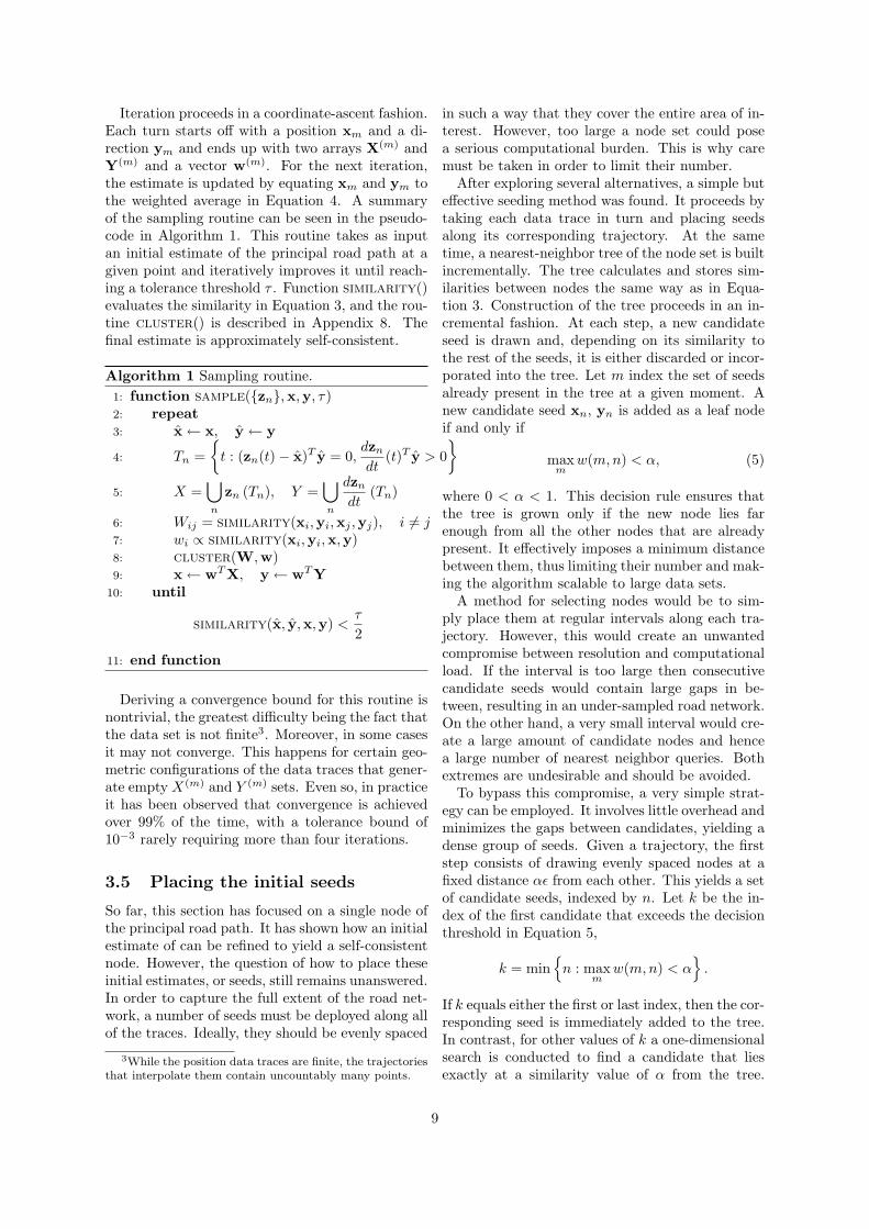
Iteration proceeds in a coordinate-ascent fashion.Each turn starts off with a position xm and a di-rection ym and ends up with two arrays X(m) andY(m) and a vector w(m). For the next iteration,the estimate is updated by equating xm and ym tothe weighted average in Equation 4. A summaryof the sampling routine can be seen in the pseudo-code in Algorithm 1. This routine takes as inputan initial estimate of the principal road path at agiven point and iteratively improves it until reach-ing a tolerance threshold τ . Function similarity()evaluates the similarity in Equation 3, and the rou-tine cluster() is described in Appendix 8. Thefinal estimate is approximately self-consistent.

Algorithm 1 Sampling routine.1: function sample({zn},x,y, τ)2: repeat3: x← x, y← y

4: Tn ={t : (zn(t)− x)T y = 0,

dzndt

(t)T y > 0}

5: X =⋃n

zn (Tn), Y =⋃n

dzndt

(Tn)

6: Wij = similarity(xi,yi,xj ,yj), i 6= j7: wi ∝ similarity(xi,yi,x,y)8: cluster(W,w)9: x← wTX, y← wTY

10: until

similarity(x, y,x,y) <τ

2

11: end function

Deriving a convergence bound for this routine isnontrivial, the greatest difficulty being the fact thatthe data set is not finite3. Moreover, in some casesit may not converge. This happens for certain geo-metric configurations of the data traces that gener-ate empty X(m) and Y (m) sets. Even so, in practiceit has been observed that convergence is achievedover 99% of the time, with a tolerance bound of10−3 rarely requiring more than four iterations.

3.5 Placing the initial seeds

So far, this section has focused on a single node ofthe principal road path. It has shown how an initialestimate of can be refined to yield a self-consistentnode. However, the question of how to place theseinitial estimates, or seeds, still remains unanswered.In order to capture the full extent of the road net-work, a number of seeds must be deployed along allof the traces. Ideally, they should be evenly spaced

3While the position data traces are finite, the trajectoriesthat interpolate them contain uncountably many points.

in such a way that they cover the entire area of in-terest. However, too large a node set could posea serious computational burden. This is why caremust be taken in order to limit their number.

After exploring several alternatives, a simple buteffective seeding method was found. It proceeds bytaking each data trace in turn and placing seedsalong its corresponding trajectory. At the sametime, a nearest-neighbor tree of the node set is builtincrementally. The tree calculates and stores sim-ilarities between nodes the same way as in Equa-tion 3. Construction of the tree proceeds in an in-cremental fashion. At each step, a new candidateseed is drawn and, depending on its similarity tothe rest of the seeds, it is either discarded or incor-porated into the tree. Let m index the set of seedsalready present in the tree at a given moment. Anew candidate seed xn, yn is added as a leaf nodeif and only if

maxm

w(m,n) < α, (5)

where 0 < α < 1. This decision rule ensures thatthe tree is grown only if the new node lies farenough from all the other nodes that are alreadypresent. It effectively imposes a minimum distancebetween them, thus limiting their number and mak-ing the algorithm scalable to large data sets.

A method for selecting nodes would be to sim-ply place them at regular intervals along each tra-jectory. However, this would create an unwantedcompromise between resolution and computationalload. If the interval is too large then consecutivecandidate seeds would contain large gaps in be-tween, resulting in an under-sampled road network.On the other hand, a very small interval would cre-ate a large amount of candidate nodes and hencea large number of nearest neighbor queries. Bothextremes are undesirable and should be avoided.

To bypass this compromise, a very simple strat-egy can be employed. It involves little overhead andminimizes the gaps between candidates, yielding adense group of seeds. Given a trajectory, the firststep consists of drawing evenly spaced nodes at afixed distance αε from each other. This yields a setof candidate seeds, indexed by n. Let k be the in-dex of the first candidate that exceeds the decisionthreshold in Equation 5,

k = min{n : max

mw(m,n) < α

}.

If k equals either the first or last index, then the cor-responding seed is immediately added to the tree.In contrast, for other values of k a one-dimensionalsearch is conducted to find a candidate that liesexactly at a similarity value of α from the tree.

9

Because the trajectory is a curve and the similar-ity metric is a continuous function, such candidatemust lie between seed k and its predecessor. There-fore, it can be found approximately using binarysearch or a standard line search routine.

Once all the seeds are in place, they are used asinitial estimates of the principal road path. Thesampling routine in Algorithm 1 is called for eachindividual seed in turn. Upon completion, a setof self-consistent road samples and a correspond-ing set of weight vectors is obtained. The set ofweight vectors, holding values that quantify the un-certainty in the association of roads to traces, areof central importance in the second stage of the al-gorithm. This stage deals with how to link nodestogether to generate the network topology and isthoroughly described in the following section.

4 Linking

The preceding section described the first stage ofthe map building algorithm. During this phase,the road network was sampled by covering it witha number of seeds that lie along the principal roadpaths. These sample nodes will now serve as anchorpoints upon which the rest of the map will be built.The next step consists of linking nodes together ina coherent manner, so as to capture the topologyof the network. The way connections are drawnis explained in this section. Basically, linking isformulated as a constrained optimization problem.Because connections are often ambiguous, not alllinks are actually needed and some must be dis-carded. In order to decide which ones to discard,the links are first ranked using a scoring criterionand then pruned incrementally according to theirscore. Details are given next.

4.1 Transition count matrix

Linking is performed by connecting nodes to oneanother with directed edges. Together, the set ofnodes and edges form a directed graph that com-prises the skeleton of the road map. The decision ofwhether two given nodes should be connected or notis based on a measure that quantifies the strengthof the connection. This measure, called the tran-sition likelihood, reflects how certain it is for thatedge to form part of the graph. A high likelihoodmeans the edge is bound to belong to the graph,whereas a low likelihood indicates that the corre-sponding nodes are weakly coupled and should notbe connected. Each pair of nodes has an edge andhence a corresponding likelihood value associatedto it. Therefore, the set of all these values can be

grouped together to form the transition matrix.Recall the intersection set defined in Equation 2.

This set is composed of all parameter values in then-th trajectory that map to points on the m-th hy-perplane with strictly positive orientation. Conse-quently, the union set⋃

m

T (m)n

comprises all intersections of trajectory n with ev-ery hyperplane. All elements in this set also possessa corresponding entry in one of the weight vectorsw(m) associated to the road nodes. Therefore, eachelement implicitly maps to the index of the nodethat was intersected, the parameter value for whichthe intersection occurred and the weight. Let

µ = {µ(k)n }, τ = {τ (k)

n }, ω = {ω(k)n },

be the set of node indices, parameter values andweights respectively for all of the elements in theunion. For convenience, all three sets can be rep-resented in a compact form by grouping them to-gether in vectors. Specifically, define the set {w(k)

n }using an m-ary coding scheme, where the m-th el-ement of vector w(k)

n is equal to 1 if ω(k)n > 0 and

m = µ(k)n , and 0 otherwise. Assume the sets are

sorted according to time, that is i ≤ j ⇒ τ(i)n ≤

τ(j)n , and define the weight matrix as the sum of

outer products of pairs of consecutive vectors

W =∑n,k

w(k−1)n w(k)T

n . (6)

Using these previous definitions, the transition ma-trix A can be expressed as the row-normalized ver-sion of the weight matrix,

A = diag (We)−1 W, (7)

where again e is the column vector with unit ele-ments. In this equation it is assumed that everyrow of W contains at least one nonzero element, sothat the inverse exists.

The transition matrix in Equation 7 is a normal-ized version of the matrix of weighted transitioncounts between road nodes. Its expression is verysimilar to the maximum likelihood estimate of thetransition matrix in a hidden Markov model. Inthis case, Aij is proportional to a sum of likelihood,each likelihood being the posterior joint probabil-ity of the previous hidden state being i and thecurrent hidden state being j. An analogy can bedrawn between the hidden Markov model and theone presented here, since the identity of the roadsamples act as latent variables. The difference be-tween the two cases is that for the road model there

10

is no ambiguity about hidden states. The reason forthis is that a trajectory almost never intersects twoor more planes simultaneously. Or in other words,it is extremely rare to find two elements in the setτn that are identical. Therefore, the joint posteriorprobability is always equal to one. This is reflectedin Equation 6, where the weight matrix is formedby accumulating products of binary vectors.

4.2 Linkage criterion

The transition matrix provides a measure of thestrength of each connection. Its support σ(A) ={(i, j) : Aij 6= 0} is a set of edges connecting nodestogether, each edge weighted by its correspondingtransition likelihood. Due to noise and ambiguitypresent in the association of traces to nodes, σ(A)may contain edges that are superfluous. Therefore,instead of incorporating all of them, only a sub-set E ⊆ σ(A) of non-superfluous edges is selected.This set constitutes the edge set of the final graph.

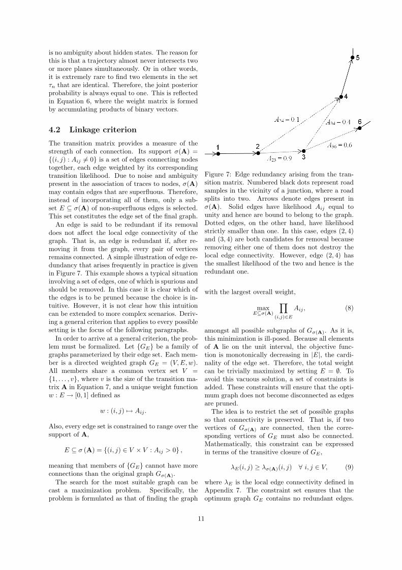
An edge is said to be redundant if its removaldoes not affect the local edge connectivity of thegraph. That is, an edge is redundant if, after re-moving it from the graph, every pair of verticesremains connected. A simple illustration of edge re-dundancy that arises frequently in practice is givenin Figure 7. This example shows a typical situationinvolving a set of edges, one of which is spurious andshould be removed. In this case it is clear which ofthe edges is to be pruned because the choice is in-tuitive. However, it is not clear how this intuitioncan be extended to more complex scenarios. Deriv-ing a general criterion that applies to every possiblesetting is the focus of the following paragraphs.

In order to arrive at a general criterion, the prob-lem must be formalized. Let {GE} be a family ofgraphs parameterized by their edge set. Each mem-ber is a directed weighted graph GE = (V,E,w).All members share a common vertex set V ={1, . . . , v}, where v is the size of the transition ma-trix A in Equation 7, and a unique weight functionw : E → [0, 1] defined as

w : (i, j) 7→ Aij .

Also, every edge set is constrained to range over thesupport of A,

E ⊆ σ (A) = {(i, j) ∈ V × V : Aij > 0} ,

meaning that members of {GE} cannot have moreconnections than the original graph Gσ(A).

The search for the most suitable graph can becast a maximization problem. Specifically, theproblem is formulated as that of finding the graph

Figure 7: Edge redundancy arising from the tran-sition matrix. Numbered black dots represent roadsamples in the vicinity of a junction, where a roadsplits into two. Arrows denote edges present inσ(A). Solid edges have likelihood Aij equal tounity and hence are bound to belong to the graph.Dotted edges, on the other hand, have likelihoodstrictly smaller than one. In this case, edges (2, 4)and (3, 4) are both candidates for removal becauseremoving either one of them does not destroy thelocal edge connectivity. However, edge (2, 4) hasthe smallest likelihood of the two and hence is theredundant one.

with the largest overall weight,

maxE⊆σ(A)

∏(i,j)∈E

Aij , (8)

amongst all possible subgraphs of Gσ(A). As it is,this minimization is ill-posed. Because all elementsof A lie on the unit interval, the objective func-tion is monotonically decreasing in |E|, the cardi-nality of the edge set. Therefore, the total weightcan be trivially maximized by setting E = ∅. Toavoid this vacuous solution, a set of constraints isadded. These constraints will ensure that the opti-mum graph does not become disconnected as edgesare pruned.

The idea is to restrict the set of possible graphsso that connectivity is preserved. That is, if twovertices of Gσ(A) are connected, then the corre-sponding vertices of GE must also be connected.Mathematically, this constraint can be expressedin terms of the transitive closure of GE ,

λE(i, j) ≥ λσ(A)(i, j) ∀ i, j ∈ V, (9)

where λE is the local edge connectivity defined inAppendix 7. The constraint set ensures that theoptimum graph GE contains no redundant edges.

11

This can be verified via the following reasoning. Ev-ery edge e = (i, j) ∈ E in the optimum graph is alsoan edge-independent path between vertices i and j.In fact, Equation 9 implies that it must be the pathwith largest weight connecting them. Should thereexist more than one edge-independent path, theymust all have weight lower than Aij . Otherwise,the objective function in Equation 8 could be in-creased by removing e from E. For this reason, ecannot be redundant.

The complete minimization problem consists ofsolving Equation 8 with respect to E, subject toEquation 9. This problem is combinatorially hardand there is no general algorithm for solving it ef-ficiently. However, it is possible to find a feasiblesuboptimal solution by means of a simple greedystrategy. By performing a locally optimal searchover possible subgraphs, the complexity becomeslinear in the number of vertices and quadratic inthe number of edges. Although complexity is stillquadratic in the worst case, the routine scales wellin practice since graphs tend to be very sparse. Fur-thermore, computation time can be minimized bytaking into account certain properties of the edgeset. A full description of the routine can be foundnext.

4.3 Suboptimal linkage

Now that the linking problem is well defined, thenext step consists of deriving an efficient methodfor solving it. Recall that each edge e = (i, j)must be the path with the largest weight betweenvertices i and j. This suggests a simple itera-tive method for monotonically increasing the over-all weight. Namely, starting from the edge e withthe largest transition likelihood, the shortest pathbetween its endpoints is computed. If this path isnot equal to e, then the edge still satisfies the con-straints in Equation 9 and hence yields a feasiblegraph. Therefore, removing it increases the overallweight in Equation 8, bringing the graph closer tothe optimum.

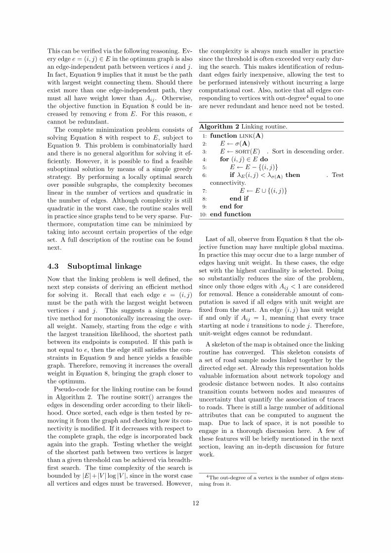
Pseudo-code for the linking routine can be foundin Algorithm 2. The routine sort() arranges theedges in descending order according to their likeli-hood. Once sorted, each edge is then tested by re-moving it from the graph and checking how its con-nectivity is modified. If it decreases with respect tothe complete graph, the edge is incorporated backagain into the graph. Testing whether the weightof the shortest path between two vertices is largerthan a given threshold can be achieved via breadth-first search. The time complexity of the search isbounded by |E|+ |V | log |V |, since in the worst caseall vertices and edges must be traversed. However,

the complexity is always much smaller in practicesince the threshold is often exceeded very early dur-ing the search. This makes identification of redun-dant edges fairly inexpensive, allowing the test tobe performed intensively without incurring a largecomputational cost. Also, notice that all edges cor-responding to vertices with out-degree4 equal to oneare never redundant and hence need not be tested.

Algorithm 2 Linking routine.1: function link(A)2: E ← σ(A)3: E ← sort(E) . Sort in descending order.4: for (i, j) ∈ E do5: E ← E − {(i, j)}6: if λE(i, j) < λσ(A) then . Test

connectivity.7: E ← E ∪ {(i, j)}8: end if9: end for

10: end function

Last of all, observe from Equation 8 that the ob-jective function may have multiple global maxima.In practice this may occur due to a large number ofedges having unit weight. In these cases, the edgeset with the highest cardinality is selected. Doingso substantially reduces the size of the problem,since only those edges with Aij < 1 are consideredfor removal. Hence a considerable amount of com-putation is saved if all edges with unit weight arefixed from the start. An edge (i, j) has unit weightif and only if Aij = 1, meaning that every tracestarting at node i transitions to node j. Therefore,unit-weight edges cannot be redundant.

A skeleton of the map is obtained once the linkingroutine has converged. This skeleton consists ofa set of road sample nodes linked together by thedirected edge set. Already this representation holdsvaluable information about network topology andgeodesic distance between nodes. It also containstransition counts between nodes and measures ofuncertainty that quantify the association of tracesto roads. There is still a large number of additionalattributes that can be computed to augment themap. Due to lack of space, it is not possible toengage in a thorough discussion here. A few ofthese features will be briefly mentioned in the nextsection, leaving an in-depth discussion for futurework.

4The out-degree of a vertex is the number of edges stem-ming from it.

12

5 Results

This section shows experimental results. A largeand rich data set is used to test the performanceof the algorithm in several different settings. Com-parisons between this and other approaches are alsopresented.

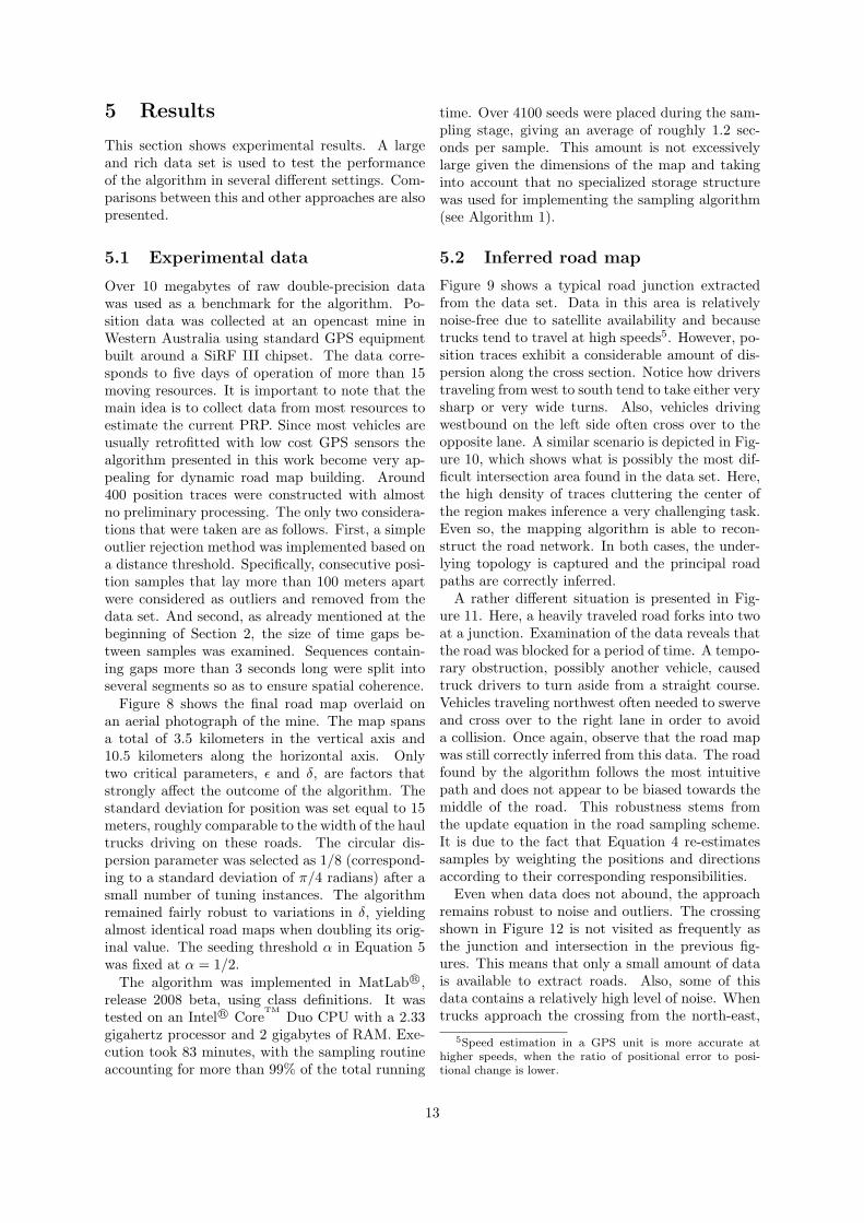
5.1 Experimental data

Over 10 megabytes of raw double-precision datawas used as a benchmark for the algorithm. Po-sition data was collected at an opencast mine inWestern Australia using standard GPS equipmentbuilt around a SiRF III chipset. The data corre-sponds to five days of operation of more than 15moving resources. It is important to note that themain idea is to collect data from most resources toestimate the current PRP. Since most vehicles areusually retrofitted with low cost GPS sensors thealgorithm presented in this work become very ap-pealing for dynamic road map building. Around400 position traces were constructed with almostno preliminary processing. The only two considera-tions that were taken are as follows. First, a simpleoutlier rejection method was implemented based ona distance threshold. Specifically, consecutive posi-tion samples that lay more than 100 meters apartwere considered as outliers and removed from thedata set. And second, as already mentioned at thebeginning of Section 2, the size of time gaps be-tween samples was examined. Sequences contain-ing gaps more than 3 seconds long were split intoseveral segments so as to ensure spatial coherence.

Figure 8 shows the final road map overlaid onan aerial photograph of the mine. The map spansa total of 3.5 kilometers in the vertical axis and10.5 kilometers along the horizontal axis. Onlytwo critical parameters, ε and δ, are factors thatstrongly affect the outcome of the algorithm. Thestandard deviation for position was set equal to 15meters, roughly comparable to the width of the haultrucks driving on these roads. The circular dis-persion parameter was selected as 1/8 (correspond-ing to a standard deviation of π/4 radians) after asmall number of tuning instances. The algorithmremained fairly robust to variations in δ, yieldingalmost identical road maps when doubling its orig-inal value. The seeding threshold α in Equation 5was fixed at α = 1/2.

The algorithm was implemented in MatLab R©,release 2008 beta, using class definitions. It wastested on an Intel R© Core

TMDuo CPU with a 2.33

gigahertz processor and 2 gigabytes of RAM. Exe-cution took 83 minutes, with the sampling routineaccounting for more than 99% of the total running

time. Over 4100 seeds were placed during the sam-pling stage, giving an average of roughly 1.2 sec-onds per sample. This amount is not excessivelylarge given the dimensions of the map and takinginto account that no specialized storage structurewas used for implementing the sampling algorithm(see Algorithm 1).

5.2 Inferred road map

Figure 9 shows a typical road junction extractedfrom the data set. Data in this area is relativelynoise-free due to satellite availability and becausetrucks tend to travel at high speeds5. However, po-sition traces exhibit a considerable amount of dis-persion along the cross section. Notice how driverstraveling from west to south tend to take either verysharp or very wide turns. Also, vehicles drivingwestbound on the left side often cross over to theopposite lane. A similar scenario is depicted in Fig-ure 10, which shows what is possibly the most dif-ficult intersection area found in the data set. Here,the high density of traces cluttering the center ofthe region makes inference a very challenging task.Even so, the mapping algorithm is able to recon-struct the road network. In both cases, the under-lying topology is captured and the principal roadpaths are correctly inferred.

A rather different situation is presented in Fig-ure 11. Here, a heavily traveled road forks into twoat a junction. Examination of the data reveals thatthe road was blocked for a period of time. A tempo-rary obstruction, possibly another vehicle, causedtruck drivers to turn aside from a straight course.Vehicles traveling northwest often needed to swerveand cross over to the right lane in order to avoida collision. Once again, observe that the road mapwas still correctly inferred from this data. The roadfound by the algorithm follows the most intuitivepath and does not appear to be biased towards themiddle of the road. This robustness stems fromthe update equation in the road sampling scheme.It is due to the fact that Equation 4 re-estimatessamples by weighting the positions and directionsaccording to their corresponding responsibilities.

Even when data does not abound, the approachremains robust to noise and outliers. The crossingshown in Figure 12 is not visited as frequently asthe junction and intersection in the previous fig-ures. This means that only a small amount of datais available to extract roads. Also, some of thisdata contains a relatively high level of noise. Whentrucks approach the crossing from the north-east,

5Speed estimation in a GPS unit is more accurate athigher speeds, when the ratio of positional error to posi-tional change is lower.

13

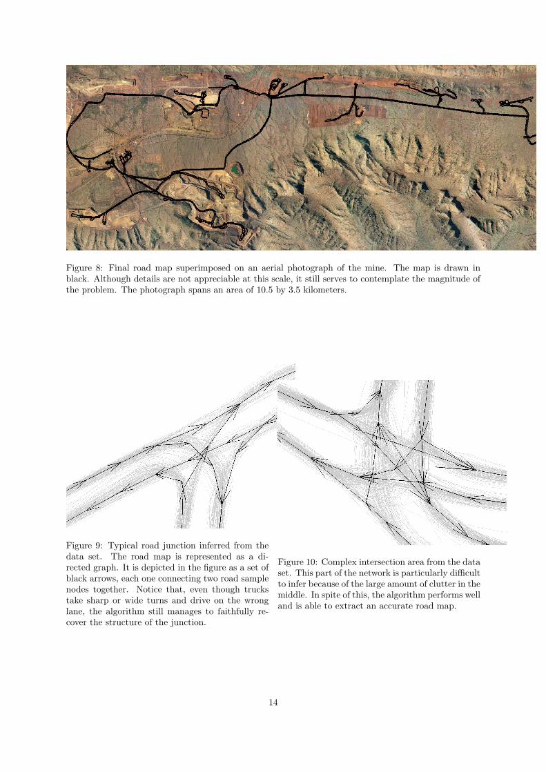
Figure 8: Final road map superimposed on an aerial photograph of the mine. The map is drawn inblack. Although details are not appreciable at this scale, it still serves to contemplate the magnitude ofthe problem. The photograph spans an area of 10.5 by 3.5 kilometers.

Figure 9: Typical road junction inferred from thedata set. The road map is represented as a di-rected graph. It is depicted in the figure as a set ofblack arrows, each one connecting two road samplenodes together. Notice that, even though truckstake sharp or wide turns and drive on the wronglane, the algorithm still manages to faithfully re-cover the structure of the junction.

Figure 10: Complex intersection area from the dataset. This part of the network is particularly difficultto infer because of the large amount of clutter in themiddle. In spite of this, the algorithm performs welland is able to extract an accurate road map.

14

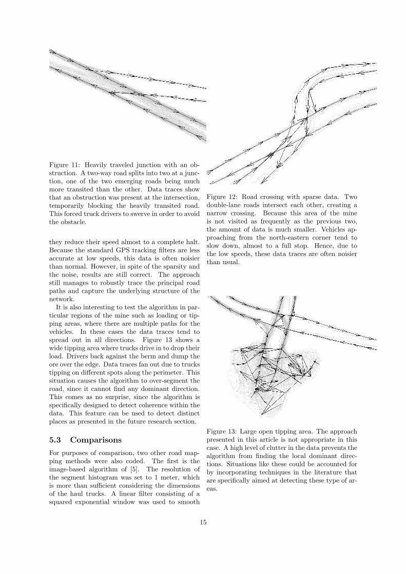
Figure 11: Heavily traveled junction with an ob-struction. A two-way road splits into two at a junc-tion, one of the two emerging roads being muchmore transited than the other. Data traces showthat an obstruction was present at the intersection,temporarily blocking the heavily transited road.This forced truck drivers to swerve in order to avoidthe obstacle.

they reduce their speed almost to a complete halt.Because the standard GPS tracking filters are lessaccurate at low speeds, this data is often noisierthan normal. However, in spite of the sparsity andthe noise, results are still correct. The approachstill manages to robustly trace the principal roadpaths and capture the underlying structure of thenetwork.

It is also interesting to test the algorithm in par-ticular regions of the mine such as loading or tip-ping areas, where there are multiple paths for thevehicles. In these cases the data traces tend tospread out in all directions. Figure 13 shows awide tipping area where trucks drive in to drop theirload. Drivers back against the berm and dump theore over the edge. Data traces fan out due to truckstipping on different spots along the perimeter. Thissituation causes the algorithm to over-segment theroad, since it cannot find any dominant direction.This comes as no surprise, since the algorithm isspecifically designed to detect coherence within thedata. This feature can be used to detect distinctplaces as presented in the future research section.

5.3 Comparisons

For purposes of comparison, two other road map-ping methods were also coded. The first is theimage-based algorithm of [5]. The resolution ofthe segment histogram was set to 1 meter, whichis more than sufficient considering the dimensionsof the haul trucks. A linear filter consisting of asquared exponential window was used to smooth

Figure 12: Road crossing with sparse data. Twodouble-lane roads intersect each other, creating anarrow crossing. Because this area of the mineis not visited as frequently as the previous two,the amount of data is much smaller. Vehicles ap-proaching from the north-eastern corner tend toslow down, almost to a full stop. Hence, due tothe low speeds, these data traces are often noisierthan usual.

Figure 13: Large open tipping area. The approachpresented in this article is not appropriate in thiscase. A high level of clutter in the data prevents thealgorithm from finding the local dominant direc-tions. Situations like these could be accounted forby incorporating techniques in the literature thatare specifically aimed at detecting these type of ar-eas.

15

the histogram. After some tuning, a width of 1.5meters was found to give the best results. The seg-mentation threshold was also selected by trial anderror, being 0.1 an acceptable value. Execution re-quired 27 minutes in total. A number of implemen-tation issues arose due to the size of the images. Toaccount for this, the algorithm was ran separatelyon a set of overlapping subregions of the image.The resulting maps were later joined together us-ing a simple data association algorithm.

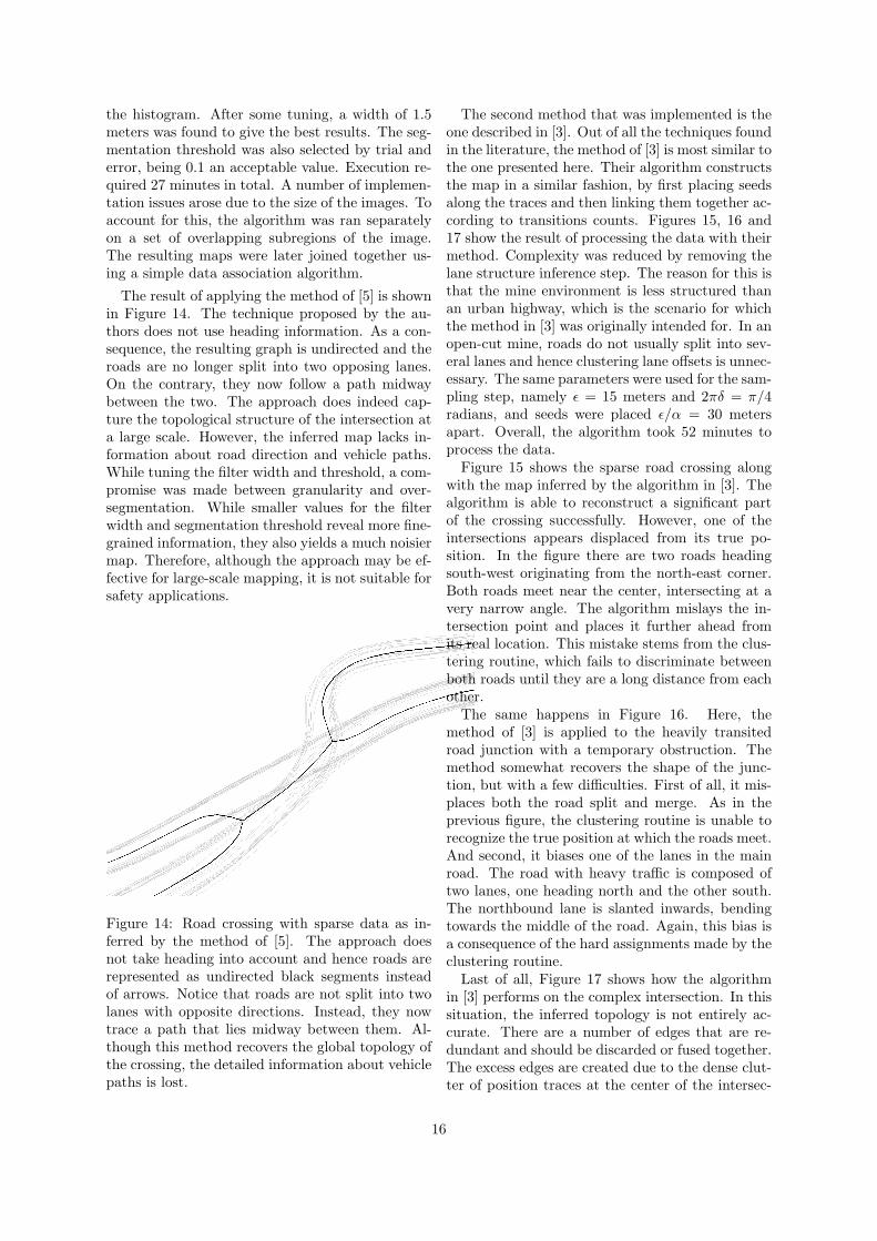
The result of applying the method of [5] is shownin Figure 14. The technique proposed by the au-thors does not use heading information. As a con-sequence, the resulting graph is undirected and theroads are no longer split into two opposing lanes.On the contrary, they now follow a path midwaybetween the two. The approach does indeed cap-ture the topological structure of the intersection ata large scale. However, the inferred map lacks in-formation about road direction and vehicle paths.While tuning the filter width and threshold, a com-promise was made between granularity and over-segmentation. While smaller values for the filterwidth and segmentation threshold reveal more fine-grained information, they also yields a much noisiermap. Therefore, although the approach may be ef-fective for large-scale mapping, it is not suitable forsafety applications.

Figure 14: Road crossing with sparse data as in-ferred by the method of [5]. The approach doesnot take heading into account and hence roads arerepresented as undirected black segments insteadof arrows. Notice that roads are not split into twolanes with opposite directions. Instead, they nowtrace a path that lies midway between them. Al-though this method recovers the global topology ofthe crossing, the detailed information about vehiclepaths is lost.

The second method that was implemented is theone described in [3]. Out of all the techniques foundin the literature, the method of [3] is most similar tothe one presented here. Their algorithm constructsthe map in a similar fashion, by first placing seedsalong the traces and then linking them together ac-cording to transitions counts. Figures 15, 16 and17 show the result of processing the data with theirmethod. Complexity was reduced by removing thelane structure inference step. The reason for this isthat the mine environment is less structured thanan urban highway, which is the scenario for whichthe method in [3] was originally intended for. In anopen-cut mine, roads do not usually split into sev-eral lanes and hence clustering lane offsets is unnec-essary. The same parameters were used for the sam-pling step, namely ε = 15 meters and 2πδ = π/4radians, and seeds were placed ε/α = 30 metersapart. Overall, the algorithm took 52 minutes toprocess the data.

Figure 15 shows the sparse road crossing alongwith the map inferred by the algorithm in [3]. Thealgorithm is able to reconstruct a significant partof the crossing successfully. However, one of theintersections appears displaced from its true po-sition. In the figure there are two roads headingsouth-west originating from the north-east corner.Both roads meet near the center, intersecting at avery narrow angle. The algorithm mislays the in-tersection point and places it further ahead fromits real location. This mistake stems from the clus-tering routine, which fails to discriminate betweenboth roads until they are a long distance from eachother.

The same happens in Figure 16. Here, themethod of [3] is applied to the heavily transitedroad junction with a temporary obstruction. Themethod somewhat recovers the shape of the junc-tion, but with a few difficulties. First of all, it mis-places both the road split and merge. As in theprevious figure, the clustering routine is unable torecognize the true position at which the roads meet.And second, it biases one of the lanes in the mainroad. The road with heavy traffic is composed oftwo lanes, one heading north and the other south.The northbound lane is slanted inwards, bendingtowards the middle of the road. Again, this bias isa consequence of the hard assignments made by theclustering routine.

Last of all, Figure 17 shows how the algorithmin [3] performs on the complex intersection. In thissituation, the inferred topology is not entirely ac-curate. There are a number of edges that are re-dundant and should be discarded or fused together.The excess edges are created due to the dense clut-ter of position traces at the center of the intersec-

16

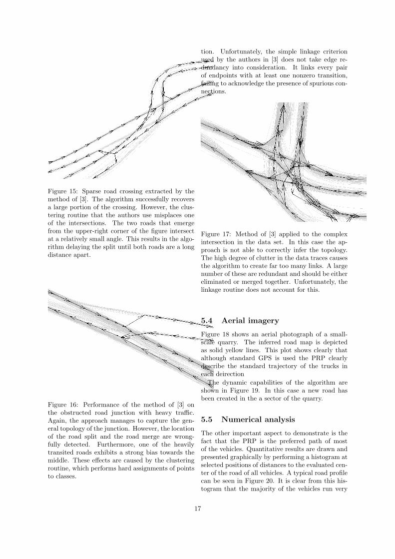
Figure 15: Sparse road crossing extracted by themethod of [3]. The algorithm successfully recoversa large portion of the crossing. However, the clus-tering routine that the authors use misplaces oneof the intersections. The two roads that emergefrom the upper-right corner of the figure intersectat a relatively small angle. This results in the algo-rithm delaying the split until both roads are a longdistance apart.

Figure 16: Performance of the method of [3] onthe obstructed road junction with heavy traffic.Again, the approach manages to capture the gen-eral topology of the junction. However, the locationof the road split and the road merge are wrong-fully detected. Furthermore, one of the heavilytransited roads exhibits a strong bias towards themiddle. These effects are caused by the clusteringroutine, which performs hard assignments of pointsto classes.

tion. Unfortunately, the simple linkage criterionused by the authors in [3] does not take edge re-dundancy into consideration. It links every pairof endpoints with at least one nonzero transition,failing to acknowledge the presence of spurious con-nections.

Figure 17: Method of [3] applied to the complexintersection in the data set. In this case the ap-proach is not able to correctly infer the topology.The high degree of clutter in the data traces causesthe algorithm to create far too many links. A largenumber of these are redundant and should be eithereliminated or merged together. Unfortunately, thelinkage routine does not account for this.

5.4 Aerial imagery

Figure 18 shows an aerial photograph of a small-scale quarry. The inferred road map is depictedas solid yellow lines. This plot shows clearly thatalthough standard GPS is used the PRP clearlydescribe the standard trajectory of the trucks ineach deirection

The dynamic capabilities of the algorithm areshown in Figure 19. In this case a new road hasbeen created in the a sector of the quarry.

5.5 Numerical analysis

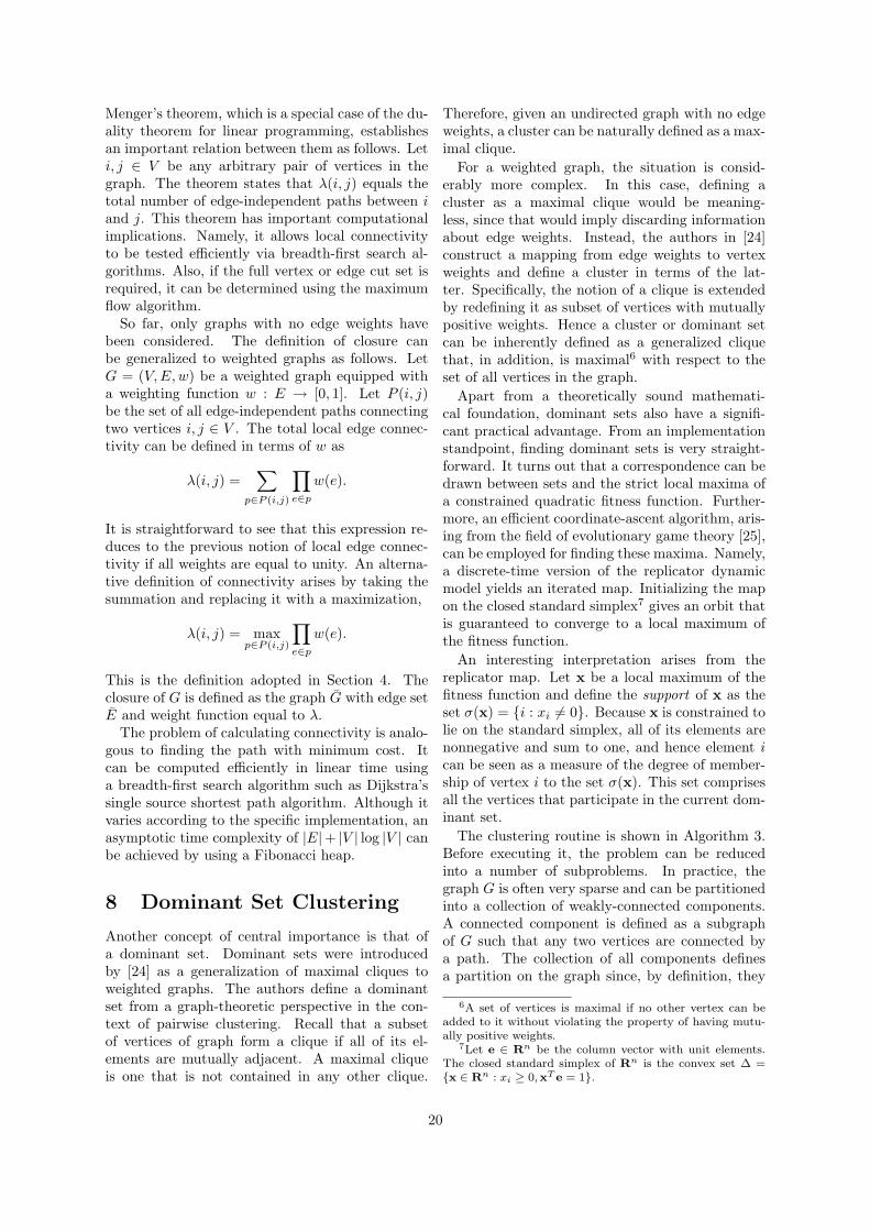
The other important aspect to demonstrate is thefact that the PRP is the preferred path of mostof the vehicles. Quantitative results are drawn andpresented graphically by performing a histogram atselected positions of distances to the evaluated cen-ter of the road of all vehicles. A typical road profilecan be seen in Figure 20. It is clear from this his-togram that the majority of the vehicles run very

17

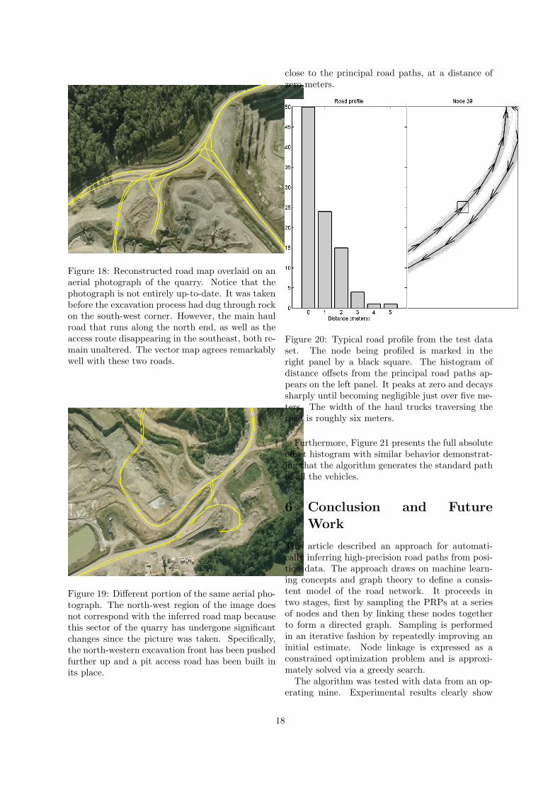
Figure 18: Reconstructed road map overlaid on anaerial photograph of the quarry. Notice that thephotograph is not entirely up-to-date. It was takenbefore the excavation process had dug through rockon the south-west corner. However, the main haulroad that runs along the north end, as well as theaccess route disappearing in the southeast, both re-main unaltered. The vector map agrees remarkablywell with these two roads.

Figure 19: Different portion of the same aerial pho-tograph. The north-west region of the image doesnot correspond with the inferred road map becausethis sector of the quarry has undergone significantchanges since the picture was taken. Specifically,the north-western excavation front has been pushedfurther up and a pit access road has been built inits place.

close to the principal road paths, at a distance ofzero meters.

Figure 20: Typical road profile from the test dataset. The node being profiled is marked in theright panel by a black square. The histogram ofdistance offsets from the principal road paths ap-pears on the left panel. It peaks at zero and decayssharply until becoming negligible just over five me-ters. The width of the haul trucks traversing theroad is roughly six meters.

Furthermore, Figure 21 presents the full absoluteoffset histogram with similar behavior demonstrat-ing that the algorithm generates the standard pathof all the vehicles.

6 Conclusion and FutureWork

This article described an approach for automati-cally inferring high-precision road paths from posi-tion data. The approach draws on machine learn-ing concepts and graph theory to define a consis-tent model of the road network. It proceeds intwo stages, first by sampling the PRPs at a seriesof nodes and then by linking these nodes togetherto form a directed graph. Sampling is performedin an iterative fashion by repeatedly improving aninitial estimate. Node linkage is expressed as aconstrained optimization problem and is approxi-mately solved via a greedy search.

The algorithm was tested with data from an op-erating mine. Experimental results clearly show

18

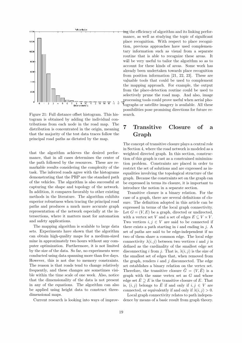
Figure 21: Full distance offset histogram. This his-togram is obtained by adding the individual con-tributions from each node in the road map. Thedistribution is concentrated in the origin, meaningthat the majority of the test data traces follow theprincipal road paths as dictated by the map.

that the algorithm achieves the desired perfor-mance, that in all cases determines the center ofthe path followed by the resources. These are re-markable results considering the complexity of thetask. The inferred roads agree with the histogramsdemonstrating that the PRP are the standard pathof the vehicles. The algorithm is also successful atcapturing the shape and topology of the network.In addition, it compares favorably to other existingmethods in the literature. The algorithm exhibitssuperior robustness when tracing the principal roadpaths and produces a much more accurate graphrepresentation of the network especially at the in-tersections, where it matters most for automationand safety applications.

The mapping algorithm is scalable to large datasets. Experiments have shown that the algorithmcan obtain high-quality maps for a medium-sizedmine in approximately two hours without any com-puter optimization. Furthermore, it is not limitedby the size of the data. So far, no experiments wereconducted using data spanning more than five days.However, this is not due to memory constraints.The reason is that roads tend to change relativelyfrequently, and these changes are sometimes visi-ble within the time scale of one week. Also, noticethat the dimensionality of the data is not presentin any of the equations. The algorithm can alsobe applied using height data to construct three-dimensional maps.

Current research is looking into ways of improv-

ing the efficiency of algorithm and its linking perfor-mance, as well as studying the topic of significantplace recognition. With respect to place recogni-tion, previous approaches have used complemen-tary information such as visual from a separateroutine that is able to recognize these areas. Itwill be very useful to tailor the algorithm so as toaccount for these kinds of areas. Some work hasalready been undertaken towards place recognitionfrom position information [21, 22, 23]. These arevaluable tools that could be used to complementthe mapping approach. For example, the outputfrom the place-detection routine could be used toselectively prune the road map. And also, imageprocessing tools could prove useful when aerial pho-tographs or satellite imagery is available. All thesepossibilities pose promising directions for future re-search.

7 Transitive Closure of aGraph

The concept of transitive closure plays a central rolein Section 4, where the road network is modeled as aweighted directed graph. In this section, construc-tion of this graph is cast as a constrained minimiza-tion problem. Constraints are placed in order torestrict the set of solutions and are expressed as in-equalities involving the topological structure of thegraph. Because the constraints set on the graph canbe expressed in terms its closure, it is important tointroduce the notion in a separate section.

Transitive closure is a binary relation. For thecase of a graph, there are several definitions of clo-sure. The definition adopted in this article can beexpressed in terms of the local graph connectivity.Let G = (V,E) be a graph, directed or undirected,with a vertex set V and a set of edges E ⊆ V × V .Two vertices i, j ∈ V are said to be connected ifthere exists a path starting in i and ending in j. Aset of paths are said to be edge-independent if notwo of them share a common edge. The local edgeconnectivity λ(i, j) between two vertices i and j isdefined as the cardinality of the smallest edge setdisconnecting i from j. That is, λ(i, j) is the size ofthe smallest set of edges that, when removed fromthe graph, renders i and j disconnected. The edgeset establishes a binary relation on the vertex set.Therefore, the transitive closure G = (V, E) is agraph with the same vertex set as G and whoseedge set E ⊇ E is the transitive closure of E. Thatis, (i, j) belongs to E if and only if i, j ∈ V areconnected, or equivalently if and only if λ(i, j) > 0.

Local graph connectivity relates to path indepen-dence by means of a basic result from graph theory.

19

Menger’s theorem, which is a special case of the du-ality theorem for linear programming, establishesan important relation between them as follows. Leti, j ∈ V be any arbitrary pair of vertices in thegraph. The theorem states that λ(i, j) equals thetotal number of edge-independent paths between iand j. This theorem has important computationalimplications. Namely, it allows local connectivityto be tested efficiently via breadth-first search al-gorithms. Also, if the full vertex or edge cut set isrequired, it can be determined using the maximumflow algorithm.

So far, only graphs with no edge weights havebeen considered. The definition of closure canbe generalized to weighted graphs as follows. LetG = (V,E,w) be a weighted graph equipped witha weighting function w : E → [0, 1]. Let P (i, j)be the set of all edge-independent paths connectingtwo vertices i, j ∈ V . The total local edge connec-tivity can be defined in terms of w as

λ(i, j) =∑

p∈P (i,j)

∏e∈p

w(e).

It is straightforward to see that this expression re-duces to the previous notion of local edge connec-tivity if all weights are equal to unity. An alterna-tive definition of connectivity arises by taking thesummation and replacing it with a maximization,

λ(i, j) = maxp∈P (i,j)

∏e∈p

w(e).

This is the definition adopted in Section 4. Theclosure of G is defined as the graph G with edge setE and weight function equal to λ.

The problem of calculating connectivity is analo-gous to finding the path with minimum cost. Itcan be computed efficiently in linear time usinga breadth-first search algorithm such as Dijkstra’ssingle source shortest path algorithm. Although itvaries according to the specific implementation, anasymptotic time complexity of |E|+ |V | log |V | canbe achieved by using a Fibonacci heap.

8 Dominant Set Clustering

Another concept of central importance is that ofa dominant set. Dominant sets were introducedby [24] as a generalization of maximal cliques toweighted graphs. The authors define a dominantset from a graph-theoretic perspective in the con-text of pairwise clustering. Recall that a subsetof vertices of graph form a clique if all of its el-ements are mutually adjacent. A maximal cliqueis one that is not contained in any other clique.

Therefore, given an undirected graph with no edgeweights, a cluster can be naturally defined as a max-imal clique.

For a weighted graph, the situation is consid-erably more complex. In this case, defining acluster as a maximal clique would be meaning-less, since that would imply discarding informationabout edge weights. Instead, the authors in [24]construct a mapping from edge weights to vertexweights and define a cluster in terms of the lat-ter. Specifically, the notion of a clique is extendedby redefining it as subset of vertices with mutuallypositive weights. Hence a cluster or dominant setcan be inherently defined as a generalized cliquethat, in addition, is maximal6 with respect to theset of all vertices in the graph.

Apart from a theoretically sound mathemati-cal foundation, dominant sets also have a signifi-cant practical advantage. From an implementationstandpoint, finding dominant sets is very straight-forward. It turns out that a correspondence can bedrawn between sets and the strict local maxima ofa constrained quadratic fitness function. Further-more, an efficient coordinate-ascent algorithm, aris-ing from the field of evolutionary game theory [25],can be employed for finding these maxima. Namely,a discrete-time version of the replicator dynamicmodel yields an iterated map. Initializing the mapon the closed standard simplex7 gives an orbit thatis guaranteed to converge to a local maximum ofthe fitness function.

An interesting interpretation arises from thereplicator map. Let x be a local maximum of thefitness function and define the support of x as theset σ(x) = {i : xi 6= 0}. Because x is constrained tolie on the standard simplex, all of its elements arenonnegative and sum to one, and hence element ican be seen as a measure of the degree of member-ship of vertex i to the set σ(x). This set comprisesall the vertices that participate in the current dom-inant set.

The clustering routine is shown in Algorithm 3.Before executing it, the problem can be reducedinto a number of subproblems. In practice, thegraph G is often very sparse and can be partitionedinto a collection of weakly-connected components.A connected component is defined as a subgraphof G such that any two vertices are connected bya path. The collection of all components definesa partition on the graph since, by definition, they

6A set of vertices is maximal if no other vertex can beadded to it without violating the property of having mutu-ally positive weights.

7Let e ∈ Rn be the column vector with unit elements.The closed standard simplex of Rn is the convex set ∆ ={x ∈ Rn : xi ≥ 0,xT e = 1}.

20

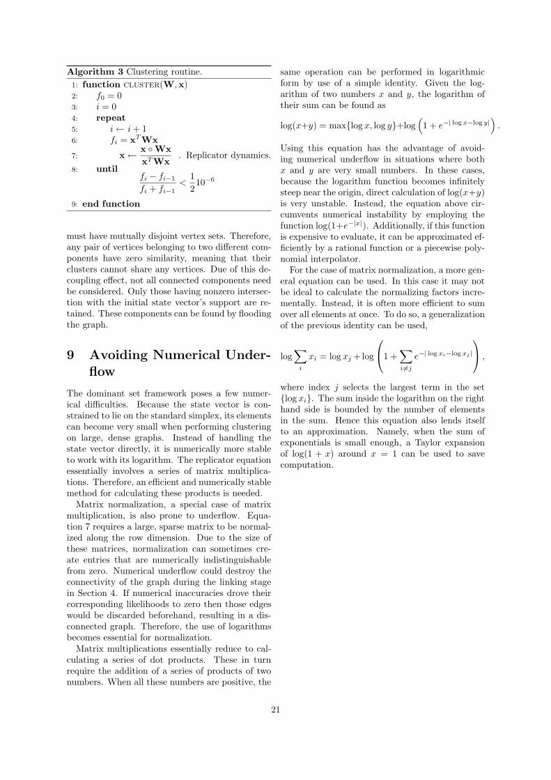
Algorithm 3 Clustering routine.1: function cluster(W,x)2: f0 = 03: i = 04: repeat5: i← i+ 16: fi = xTWx

7: x← x ◦WxxTWx

. Replicator dynamics.8: until

fi − fi−1

fi + fi−1<

12

10−6

9: end function

must have mutually disjoint vertex sets. Therefore,any pair of vertices belonging to two different com-ponents have zero similarity, meaning that theirclusters cannot share any vertices. Due of this de-coupling effect, not all connected components needbe considered. Only those having nonzero intersec-tion with the initial state vector’s support are re-tained. These components can be found by floodingthe graph.

9 Avoiding Numerical Under-flow

The dominant set framework poses a few numer-ical difficulties. Because the state vector is con-strained to lie on the standard simplex, its elementscan become very small when performing clusteringon large, dense graphs. Instead of handling thestate vector directly, it is numerically more stableto work with its logarithm. The replicator equationessentially involves a series of matrix multiplica-tions. Therefore, an efficient and numerically stablemethod for calculating these products is needed.

Matrix normalization, a special case of matrixmultiplication, is also prone to underflow. Equa-tion 7 requires a large, sparse matrix to be normal-ized along the row dimension. Due to the size ofthese matrices, normalization can sometimes cre-ate entries that are numerically indistinguishablefrom zero. Numerical underflow could destroy theconnectivity of the graph during the linking stagein Section 4. If numerical inaccuracies drove theircorresponding likelihoods to zero then those edgeswould be discarded beforehand, resulting in a dis-connected graph. Therefore, the use of logarithmsbecomes essential for normalization.

Matrix multiplications essentially reduce to cal-culating a series of dot products. These in turnrequire the addition of a series of products of twonumbers. When all these numbers are positive, the

same operation can be performed in logarithmicform by use of a simple identity. Given the log-arithm of two numbers x and y, the logarithm oftheir sum can be found as

log(x+y) = max{log x, log y}+log(

1 + e−| log x−log y|).

Using this equation has the advantage of avoid-ing numerical underflow in situations where bothx and y are very small numbers. In these cases,because the logarithm function becomes infinitelysteep near the origin, direct calculation of log(x+y)is very unstable. Instead, the equation above cir-cumvents numerical instability by employing thefunction log(1+e−|x|). Additionally, if this functionis expensive to evaluate, it can be approximated ef-ficiently by a rational function or a piecewise poly-nomial interpolator.

For the case of matrix normalization, a more gen-eral equation can be used. In this case it may notbe ideal to calculate the normalizing factors incre-mentally. Instead, it is often more efficient to sumover all elements at once. To do so, a generalizationof the previous identity can be used,

log∑i

xi = log xj + log

1 +∑i 6=j

e−| log xi−log xj |

,

where index j selects the largest term in the set{log xi}. The sum inside the logarithm on the righthand side is bounded by the number of elementsin the sum. Hence this equation also lends itselfto an approximation. Namely, when the sum ofexponentials is small enough, a Taylor expansionof log(1 + x) around x = 1 can be used to savecomputation.

21

References

[1] C. Wilson, S. Rogers, and S. Weisenburger,“The potential of precision maps in intelligentvehicles,” in Proceedings of the 1998 IEEE In-ternational Conference on Intelligent Vehicles,1998, pp. 419–422.

[2] S. Edelkamp and S. Schrodl, “Route plan-ning and map inference with global positioningtraces,” Computer Science in Perspective: Es-says Dedicated to Thomas Ottmann, vol. -, pp.128–151, 2003.

[3] S. Schroedl, K. Wagstaff, S. Rogers, P. Lan-gley, and C. Wilson, “Mining gps traces formap refinement,” Transactions on Data Min-ing and Knowledge Discovery, vol. 9, no. 1, pp.59–87, 2004.

[4] R. Bruntrup, S. Edelkamp, S. Jabbar, andB. Scholz, “Incremental map generation withgps traces,” in Proceedings of the 2005 IEEEInternational Conference on Intelligent Trans-portation Systems, Sept. 2005, pp. 574–579.

[5] J. Davies, A. Beresford, and A. Hopper, “Scal-able, distributed, real-time map generation,”IEEE Transactions on Pervasive Computing,vol. 5, no. 4, pp. 47–54, Oct.-Dec. 2006.

[6] S. Worrall, “Providing situation awareness incomplex multi-vehicle operations,” Ph.D. dis-sertation, School of Aerospace, Mechanic andMechatronic Engineering, July 2009.

[7] S. Worrall and E. Nebot, “Using non-parametric filters and sparse observations tolocalise a fleet of mining vehicles,” in Proceed-ings of the 2007 IEEE International Confer-ence on Robotics and Automation, April 2007,pp. 509–516.

[8] ——, “A probabilistic method for detectingimpending vehicle interactions,” in Proceed-ings of the 2008 IEEE International Confer-ence on Robotics and Automation, May 2008,pp. 1787–1791.

[9] M. Negri, P. Gamba, G. Lisini, and F. Tupin,“Junction-aware extraction and regularizationof urban road networks in high-resolution sarimages,” IEEE Transactions on Geoscienceand Remote Sensing, vol. 44, no. 10, pp. 2962–2971, October 2006.

[10] P. Gamba, F. Dell’Acqua, and G. Lisini,“Improving urban road extraction in high-resolution images exploiting directional filter-

ing, perceptual grouping, and simple topolog-ical concepts,” IEEE Geoscience and RemoteSensing Letters, vol. 3, no. 3, pp. 387–391, July2006.

[11] J. Hu, A. Razdan, J. Femiani, M. Cui, andP. Wonka, “Road network extraction and in-tersection detection from aerial images bytracking road footprints,” IEEE Transactionson Geoscience and Remote Sensing, vol. 45,no. 12, pp. 4144–4157, December 2007.

[12] M. Amo, F. Martinez, and M. Torre, “Roadextraction from aerial images using a regioncompetition algorithm,” IEEE Transactionson Image Processing, vol. 15, no. 5, pp. 1192–1201, May 2006.

[13] R. Stoica, X. Descombes, and J. Zerubia, “Agibbs point process for road extraction from re-motely sensed images,” International Journalof Computer Vision, vol. 57, no. 2, pp. 121–136, 2004.

[14] S. Rogers, P. Langley, and C. Wilson, “Mininggps data to augment road models,” in Proceed-ings of the Fifth ACM International Confer-ence on Knowledge Discovery and Data Min-ing. New York, NY, USA: ACM, 1999, pp.104–113.

[15] M. Drozdzynski, S. Edelkamp, A. Gaubatz,S. Jabbar, and M. Liebe, “On constructing abase map for collaborative map generation andits application in urban mobility planning,”in Proceedings of the 2007 IEEE InternationalConference on Intelligent Transportation Sys-tems, 30 2007-Oct. 3 2007, pp. 678–683.

[16] S. Edelkamp, S. Jabbar, and T. Willhalm,“Geometric travel planning,” IEEE Transac-tions on Intelligent Transportation Systems,vol. 6, no. 1, pp. 5–16, March 2005.

[17] J. Roth, “Extracting line string features fromgps logs,” in 5. GI/ITG KuVS Fachgesprach“Ortsbezogene Anwendungen und Dienste”.University of Applied Sciences, Nurnberg: Sci-entific Series Offprint, 2008, pp. 41–46.

[18] T. Hastie and W. Stuetzle, “Principal curves,”Journal of the American Statistical Associa-tion, vol. 84, no. 406, pp. 502–516, June 1989.

[19] H. Alt and M. Godau, “Computing the frechetdistance between two polygonal curves,” Inter-national Journal of Computational Geometryand Applications, vol. 5, no. 1–2, pp. 75–91,1995.

22

[20] B. Kegl, A. Krzyzak, T. Linder, and K. Zeger,“A polygonal line algorithm for constructingprincipal curves,” in Proceedings of the 1998International Conference on Advances in Neu-ral Information Processing Systems. Cam-bridge, MA, USA: MIT Press, 1999, pp. 501–507.

[21] D. Ashbrook and T. Starner, “Using gps tolearn significant locations and predict move-ment across multiple users,” Personal andUbiquitous Computing, vol. 7, no. 5, pp. 275–286, 2003.

[22] L. Liao, D. Fox, and H. Kautz, “Extractingplaces and activities from gps traces using hi-erarchical conditional random fields,” Interna-tional Journal of Robotics Research, vol. 26,no. 1, pp. 119–134, 2007.

[23] G. Agamennoni, J. Nieto, and E. Nebot, “Min-ing gps data for extracting significant places,”in Proceedings of the 2008 IEEE InternationalConference on Robotics and Automation, 2008.

[24] M. Pavan and M. Pelillo, “Dominant setsand pairwise clustering,” IEEE Transactionson Pattern Analysis and Machine Intelligence,vol. 29, no. 1, pp. 167–172, 2007.

[25] J. Weibull, Evolutionary Game Theory. TheMIT Press, August 1995.

23