Technical Report Documentation Page 1. Report No. 2 ... · TRUCK INSTRUMENTATION FOR DYNAMIC LOAD...

Technical Report Documentation . Report No. FHWA/TX-06/0-4863-1

2. Government Accession No.

3. Recipient's Catalog No. 5. Report Date

August 2006 Published: December 2007

4. Title and Subtitle

TRUCK INSTRUMENTATION FOR DYNAMIC LOAD MEASUREMENT

6. Performing Organization Code

7. Author(s) Emmanuel Fernando, Gerry Harrison, and Stacy Hilbrich

8. Performing Organization Report No. Report 0-4863-1 10. Work Unit No. (TRAIS)

9. Performing Organization Name and Address

Texas Transportation Institute The Texas A&M University System College Station, Texas 77843-3135

11. Contract or Grant No. Project 0-4863 13. Type of Report and Period Covered

Technical Report: September 2004 B July 2006

12. Sponsoring Agency Name and Address

Texas Department of Transportation Research and Technology Implementation Office P. O. Box 5080 Austin, Texas 78763-5080

14. Sponsoring Agency Code

15. Supplementary Notes

Project performed in cooperation with the Texas Department of Transportation and the Federal Highway Administration. Project Title: Characterizing the Effects of Surface Roughness on Vehicle Dynamic Loads and Pavement Life URL: http://tti.tamu.edu/documents/0-4863-1.pdf 16. Abstract

The Texas Department of Transportation (TxDOT) is implementing a ride specification that uses profile data collected with inertial profilers for acceptance testing of the finished surface. This specification is based primarily on ride quality criteria. The objective of the present project is to establish whether gaps exist in the current specification that permit frequency components of surface profile to pass that are potentially detrimental to pavement life based on the induced dynamic loading. To carry out this objective, the work plan includes tests to measure surface profiles and vehicle dynamic loads on in-service pavement sections. This interim report documents the research efforts conducted to provide an instrumented tractor-semitrailer combination for measurement of dynamic loads and a high-speed inertial profiler for measurement of surface profiles. These test vehicles were used in this project to collect data for evaluating TxDOT’s Item 585 ride specification. 17. Key Words Surface Roughness, Vehicle Dynamic Loads, Truck Instrumentation, Profile Measurement, Inertial Profiler, Strain Gages

18. Distribution Statement No restrictions. This document is available to the public through NTIS: National Technical Information Service Springfield, VA 22161 http://www.ntis.gov

19. Security Classif.(of this report) Unclassified

20. Security Classif.(of this page) Unclassified

21. No. of Pages

80

22. Price

Form DOT F 1700.7 (8-72) Reproduction of completed page authorized

http://www.ntis.gov

TRUCK INSTRUMENTATION FOR DYNAMIC LOAD MEASUREMENT

by Emmanuel Fernando Research Engineer Texas Transportation Institute Gerry Harrison Research Technician Texas Transportation Institute

and

Stacy Hilbrich Assistant Research Engineer

Texas Transportation Institute

Report 0-4863-1 Project 0-4863

Project Title: Characterizing the Effects of Surface Roughness on Vehicle Dynamic Loads and Pavement Life

Performed in cooperation with the Texas Department of Transportation and the Federal Highway Administration August 2006

Published: December 2007

TEXAS TRANSPORTATION INSTITUTE The Texas A&M University System College Station, Texas 77843-3135

v

DISCLAIMER

The contents of this report reflect the views of the authors, who are responsible for the

facts and the accuracy of the data presented. The contents do not necessarily reflect the

official views or policies of the Texas Department of Transportation (TxDOT) or the Federal

Highway Administration (FHWA). This report does not constitute a standard, specification,

or regulation, nor is it intended for construction, bidding, or permit purposes. The United

States Government and the State of Texas do not endorse products or manufacturers. Trade

or manufacturers‘ names appear herein solely because they are considered essential to the

object of this report. The engineer in charge of the project was Dr. Emmanuel G. Fernando,

P.E. # 69614.

vi

ACKNOWLEDGMENTS

The work reported herein was conducted as part of a research project sponsored by the

Texas Department of Transportation and the Federal Highway Administration. The authors

gratefully acknowledge the support and technical guidance of the project director, Mr. Brian

Michalk, of the Materials and Pavements Section of TxDOT. In addition, the authors give

special thanks to Dr. Roger Walker of the University of Texas at Arlington for his help in

profile instrumentation. His contributions are sincerely appreciated.

vii

TABLE OF CONTENTS Page LIST OF FIGURES ............................................................................................................... viii LIST OF TABLES.....................................................................................................................x CHAPTER

I INTRODUCTION ........................................................................................................1

II DEVELOPMENT OF METHODOLOGY FOR TRUCK INSTRUMENTATION TO MEASURE DYNAMIC LOADS....................................3

Strain Gage Principles ..............................................................................................3 Shear Beam Load Cell Experiment ..........................................................................7 Small-Scale Testing with an Instrumented Trailer .................................................10 Instrumentation and Calibration of Tractor-Semitrailer Combination...................18

III FABRICATION AND VERIFICATION OF INERTIAL

PROFILING SYSTEM...............................................................................................35

IV SUMMARY OF FINDINGS ......................................................................................43 REFERENCES ........................................................................................................................45 APPENDIX

LITERATURE REVIEW ....................................................................................................47

Truck Tests to Investigate Relationships between Pavement Roughness, Vehicle Characteristics, and Dynamic Tire Loads .................................................47

Indices Characterizing Truck Dynamic Loading........................................................51 Truck Tests on Instrumented Pavement Sections .......................................................62 Truck Surveys .............................................................................................................66

viii

LIST OF FIGURES Figure Page

2.1 Diagram of an Electrical-Resistance Strain Gage.........................................................5 2.2 Wheatstone Bridge Circuit with Constant Voltage Excitation .....................................6 2.3 Shear Strain Gage Used for Tests .................................................................................9 2.4 Shear Beam Load Cell Experimental Setup................................................................10 2.5 Small-Scale Trailer Used to Verify Strain Measurement Methodology.....................11 2.6 Strain Gages Positioned between Suspension and Tire of Small Trailer ...................12 2.7 Load Cell Placed under Tire during Calibration of Small Trailer ..............................14 2.8 Data from Laboratory Calibration of Small Trailer....................................................14 2.9 Dynamic Loads on Left Tire from Run 1 of Small Trailer on SH6 WIM Site...........15 2.10 Dynamic Loads on Left Tire from Run 2 of Small Trailer on SH6 WIM Site...........15 2.11 Dynamic Loads on Left Tire from Run 3 of Small Trailer on SH6 WIM Site...........16 2.12 Dynamic Loads on Left Tire from Run 4 of Small Trailer on SH6 WIM Site...........16 2.13 Dynamic Loads on Left Tire from Run 5 of Small Trailer on SH6 WIM Site...........17 2.14 Instrumentation and Calibration of Test Vehicle in the Laboratory...........................19 2.15 Layout of Sensors, Signal Conditioning, and Data Acquisition Devices on

Instrumented Truck.....................................................................................................20 2.16 Strain Gage Mounted on Trailer Axle ........................................................................22 2.17 Strain Gage Mounted on Drive Axle ..........................................................................23 2.18 Application of Load to Axle Assembly through Loading Plate .................................24 2.19 Load Cells Positioned under Dual Tires of Trailer Axle Assembly ...........................25 2.20 Calibration Results for Load Cell #1 ..........................................................................26 2.21 Calibration Results for Load Cell #2 ..........................................................................26 2.22 Calibration Results for Load Cell #3 ..........................................................................27 2.23 Calibration Results for Load Cell #4 ..........................................................................27 2.24 Strain Gage Calibration Curve for Left Side of Trailer Lead Axle ............................29 2.25 Strain Gage Calibration Curve for Right Side of Trailer Lead Axle ..........................29 2.26 Strain Gage Calibration Curve for Left Side of Second Trailer Axle ........................30 2.27 Strain Gage Calibration Curve for Right Side of Second Trailer Axle ......................30 2.28 Strain Gage Calibration Curve for Left Side of Drive Lead Axle ..............................31 2.29 Strain Gage Calibration Curve for Right Side of Drive Lead Axle............................31 2.30 Strain Gage Calibration Curve for Left Side of Drive Trailing Axle .........................32 2.31 Strain Gage Calibration Curve for Right Side of Drive Trailing Axle.......................32 2.32 Strain Gage Calibration Curve for Left Side of Steering Axle...................................33 2.33 Strain Gage Calibration Curve for Right Side of Steering Axle.................................34 3.1 Laser/Accelerometer Modules Mounted in Front of Test Vehicle .............................36 3.2 Repeatability of Profiles Measured on Left Wheel Path of Smooth Section..............38 3.3 Repeatability of Profiles Measured on Right Wheel Path of Smooth Section ...........38 3.4 Repeatability of Profiles Measured on Left Wheel Path of

Medium Smooth Section.............................................................................................39 3.5 Repeatability of Profiles Measured on Right Wheel Path of

Medium Smooth Section.............................................................................................39

ix

LIST OF FIGURES (CONT.) Figure Page

A1 Predicted Dynamic Loads on a Smooth Pavement (SI = 4.5).....................................52 A2 Predicted Dynamic Loads on a Medium-Smooth Pavement (SI = 3.4)......................52 A3 Predicted Dynamic Loads on a Rough Pavement (SI = 2.5) ......................................53 A4 Illustration of Approach Used to Evaluate Initial Overlay Smoothness.....................54

x

LIST OF TABLES Table Page

2.1 Comparison of Vertical Dynamic Tire Loads.............................................................18 3.1 Repeatability of Profile Measurements from TTI Profiler .........................................40 3.2 Repeatability of IRIs from Profile Measurements with TTI Profiler .........................40 3.3 Accuracy of Profile Measurements from TTI Profiler ...............................................40 3.4 Accuracy of IRIs from Profile Measurements with TTI Profiler ...............................40 3.5 Highways Where Researchers Collected Profile and Dynamic

Load Measurements ....................................................................................................41 A1 Summary of t-test on Difference in Truck Tire Inflation Pressures

between Loaded and Empty Trucks (Wang and Machemehl, 2000)..........................68 A2 One-Way ANOVA Results from Test of Difference in Tire

Inflation Pressures between Border and Non-Border Areas (Wang and Machemehl, 2000) .........................................................................69

A3 Two-Way ANOVA Results for Geographic Area and Highway Class (Wang and Machemehl, 2000) ..........................................................................69

A4 One-Way ANOVA Results for Different Truck Axles (Wang and Machemehl, 2000)....................................................................................69

1

CHAPTER I. INTRODUCTION

The Texas Department of Transportation (TxDOT) is implementing a new ride

specification that uses profile data collected with inertial profilers for acceptance testing of

the finished surface. Supplemental specification (SS) 5880 or the standard specification,

Item 585, is applicable for either hot-mix asphalt or Portland cement concrete pavements.

TxDOT began implementing SS 5880 in 2002. In 2003, TxDOT adopted a modified version

of this smoothness specification as the standard (Item 585), and approved its publication in

the 2004 standard specifications.

Both SS 5880 and Item 585 incorporate criteria on section smoothness and localized

roughness to evaluate the acceptability of the finished surface. Section smoothness is

evaluated at 0.1-mile intervals using the international roughness index (IRI) computed from

measured profiles. In this evaluation, the average of the left and right wheel path IRIs is

computed and used in the appropriate schedule to determine the pay adjustment for a given

0.1-mile section. To evaluate localized roughness, the specifications look at the differences

between the average profile and its 25-ft moving average to locate bumps and dips following

a modified procedure based on the methodology proposed by Fernando and Bertrand (2002).

The new standard smoothness specification (Item 585) includes pay adjustments that

relate to the ride quality achieved from construction. Since the specification is based

primarily on ride quality, a question to ask is, “Are there profile components not accounted

for that might be detrimental to pavement life based on dynamic loading criteria?” The

present research aims to answer this question by investigating the relationship between

surface roughness and truck dynamic loads. The objective is to establish whether gaps exist

in the current ride quality criteria implemented in Item 585 that permit frequency

components of surface profile to pass that are potentially detrimental to pavement life based

on the induced dynamic loading. To carry out this objective, the work plan for this project

includes tests to measure surface profiles and vehicle dynamic loads on in-service pavement

sections. For these tests, researchers instrumented a truck with sensors for measurement of

dynamic loads and put together an inertial profiler system for measurement of surface

profiles. This interim report documents the instrumentation program carried out by

researchers. It is organized into the following chapters:

2

• Chapter I provides a brief introduction on the rationale for this project.

• Chapter II documents the truck instrumentation for measurement of dynamic

loads. It presents the methodology implemented for these measurements,

preliminary tests conducted to verify and develop the methodology, sensor

installation, and laboratory calibrations conducted to establish calibration curves

relating sensor output to measured tire loads.

• Chapter III presents the results from field tests conducted to verify the

measurements from a test vehicle instrumented with an inertial profiling system at

the Texas Transportation Institute (TTI). This test vehicle was used in this project

to collect profile measurements for the purpose of evaluating TxDOT’s current

Item 585 ride specification. Prior to these measurements, researchers tested the

profiler and verified that it met the certification requirements specified in TxDOT

Test Method Tex-1001S.

• Chapter IV summarizes the findings from the instrumentation program.

The appendix presents the literature review conducted by researchers to gather information

on the following subject areas relevant to this project:

• measurement of vehicle dynamic loads,

• truck surveys identifying truck configurations commonly used by carriers to

transport goods and commodities,

• smoothness statistics for characterizing pavement smoothness based on truck

damage criteria,

• vehicle transfer functions, and

• compilations of data on truck geometric, mass, and suspension properties.

3

CHAPTER II. DEVELOPMENT OF METHODOLOGY FOR TRUCK INSTRUMENTATION TO MEASURE DYNAMIC LOADS

The literature review conducted in this project identified strain gages as a method for

instrumenting vehicles to measure dynamic loads. To use strain gages for this application,

researchers:

• reviewed principles of strain gage measurement,

• conducted laboratory tests to verify their application, and

• performed small-scale experiments with an instrumented trailer to verify procedures

for strain gage calibration and test a system for collecting dynamic load

measurements.

This staged approach led to the instrumentation and calibration of a test vehicle that is

presented in this chapter.

STRAIN GAGE PRINCIPLES

Engineering design requires information on the stresses and deformations that a

structure or structural member are expected to sustain during service. For many design

problems, mechanics of materials give a basis for predicting the structural response to service

loads. Indeed, solutions for stresses and deformations induced under typical design loadings

for simple structural members are found in the literature, and, for more complicated

geometric and loading configurations, numerical techniques are available. Still, many

engineering problems are encountered in practice where theoretical analysis may not be

sufficient, and experimental measurements are required to verify theoretical predictions or to

obtain actual measurements from laboratory or full-scale models. In most cases, force or

stress cannot be measured directly, but the deformations they generate can. Thus, when an

object is weighed on a scale, it is the extension of the spring that is measured, and the weight

is calculated using Hooke’s law with the measured spring displacement. In a similar manner,

load cells have sensors that measure the deformations induced under loading that relate to the

magnitude of the applied load. When the deformation is defined as the change in length per

unit length of a given object, it is called strain. Of the strain-measuring systems that are

available for practical applications, the most frequently used device for strain measurement is

the electrical-resistance strain gage.

4

The term “strain gage” usually refers to a thin wire or foil, folded back and forth on

itself to form a grid pattern, as illustrated in Figure 2.1. The grid pattern maximizes the

amount of metallic wire or foil subject to strain in the parallel direction. The grid is bonded

to a thin backing, called the carrier, which is attached directly to the test specimen.

Therefore, the strain experienced by the test specimen is transferred directly to the strain

gauge, which responds with a linear change in electrical resistance.

The discovery of the principle upon which the electrical-resistance strain gage is

based was made in 1856 by Lord Kelvin, who observed from an experiment that the

resistance of a wire increases with increasing strain according to the relationship (Dally and

Riley, 1978)

R LA

= ρ (2.1)

where R is the measured resistance in the wire of length L and cross-sectional area A having a

specific resistance ρ. From this relationship, it can be shown that the strain sensitivity of any

conductor derives from the change in its dimensions during loading and the change in

specific resistance according to the relation

dR R d/ /ε

ν ρ ρε

= + +1 2 (2.2)

where ν is the Poisson’s ratio of the conductor, ε is the strain and the other terms are as

previously defined. In practice, the strain sensitivity is also referred to as the gage factor Sg.

Thus:

S dR R R Rg = ≈

/ /ε ε

∆ (2.3)

For most alloys, the gage factor varies from about 2 to 4 (Dally and Riley, 1978). Most

strain gages are fabricated from a 45% nickel – 55% copper alloy known as Constantan,

which has a gage factor of approximately 2. This alloy exhibits several characteristics that

are useful for engineering applications. Among these are:

• The strain sensitivity is linear over a wide range of strain;

• The strain sensitivity does not change as the material goes plastic, permitting

measurements of strain in both the elastic and plastic ranges of most materials;

• The alloy has a low temperature coefficient, which reduces the temperature sensitivity

of the strain gage; and

5

Figure 2.1. Diagram of an Electrical-Resistance Strain Gage.

• The temperature properties of selected melts of the alloy permit the production of

temperature-compensated strain gages for a variety of materials on which the gages

are commonly used.

In practice, the application of strain gages will require measurement of the resistance

change and its conversion to strain using Eq. (2.3). This conversion is made with the gage

factor that is supplied by the manufacturer of the particular sensor used in the experiment.

Since the strains to be measured are typically within a few milli-strains, the resistance

changes are usually too small to be measured with a simple ohmmeter. For example, at

1 percent strain, the resistance change would be only 2 percent for a sensor with a gage factor

of 2. In practice, much smaller strains have to be measured. Thus, the application of strain

gages will require accurate measurement of very small changes in resistance. To accomplish

these measurements, a Wheatstone bridge is typically used. This method permits both static

and dynamic strain gage measurements. It is interesting to note that this is the same method

Lord Kelvin used to measure resistance changes in the classic experiment he conducted in the

mid-19th century.

Figure 2.2 illustrates the Wheatstone bridge circuit. Up to four strain gages may be

connected to the four arms of the bridge. When the gage resistance is changed by strain, the

bridge becomes unbalanced, resulting in a voltage change that is easily measured. For a

Wheatstone bridge with a constant voltage excitation V and resistances R1, R2, R3, and R4, the

6

Figure 2.2. Wheatstone Bridge Circuit with Constant Voltage Excitation.

voltage change ∆E is related to the change in resistance ∆Ri in each bridge arm i by the

relation (Dally and Riley, 1978):

∆∆ ∆ ∆ ∆E V R R

R RR

RR

RR

RR

R=

+− + −

⎛⎝⎜

⎞⎠⎟1 2

1 22

1

1

2

2

3

3

4

4( ) (2.4)

For a multiple gage circuit with n gages (n = 1, 2, 3, or 4) whose outputs sum when placed in

the bridge circuit, Eq. (2.4) can be rewritten as

∆∆E V R R

R Rn R

R=

+1 2

1 22( )

(2.5)

7

where ∆R is the change in the bridge resistance and R is the nominal resistance of the bridge

elements. The bridge circuit sensitivity Sc is defined as the change in voltage per unit strain.

Setting r = R1/R2, this parameter is determined from Eqs. (2.3) and (2.5) as follows:

S E V rr

n Sc g= =+

∆ε ( )1 2 (2.6)

It can be shown that the maximum circuit sensitivity is achieved when r = 1. With one strain

gage connected to the Wheatstone bridge, Eq. (2.6) gives the sensitivity of this configuration

as Sg V/4, compared to a sensitivity of Sg V for a four-arm active configuration. The four-arm

active bridge is of particular interest as it was the bridge configuration used for dynamic load

measurements with the instrumented tractor-semitrailer in this project. In addition to

providing the highest sensitivity, this bridge arrangement is also temperature-compensated

and rejects both axial and bending strains for applications involving shear strain

measurement. For this bridge configuration, the strain corresponding to the measured

voltage change in the Wheatstone bridge is determined from the formula:

ε =∆ES Vg

(2.7)

Prior to instrumenting a tractor-semitrailer with strain gages for dynamic load measurements,

researchers conducted laboratory and field tests to verify the application of the strain gage

principles presented in this section. Specifically, the researchers verified the principles

presented in the laboratory through an experiment that they conducted with a simple shear

beam load cell. Following up on this experiment, researchers instrumented and conducted

laboratory and field tests on a small trailer to verify the intended method of measuring

dynamic loads using shear strain gages. The tests performed are presented in the subsequent

sections.

SHEAR BEAM LOAD CELL EXPERIMENT

For a prismatic cantilevered beam of solid rectangular cross-section with a load W at

its free end, the shear stress τ at any given cross-section along its length is given by the

formula

τ =W QI b

(2.8)

where

8

Q = area moment about the neutral axis,

I = moment of inertia about the neutral axis, and

b = width of the beam.

For a solid rectangular cross-section of width b and height h, Q and I are given by the

following equations:

Q bh=

2

8 (2.9)

I bh=

3

12 (2.10)

Substituting Eqs. (2.9) and (2.10) in Eq. (2.8) and considering that the shear stress τ equals

the shear modulus G multiplied by the shear strain γ, the following equation for computing

the load W is obtained:

W bhG=

23

γ (2.11)

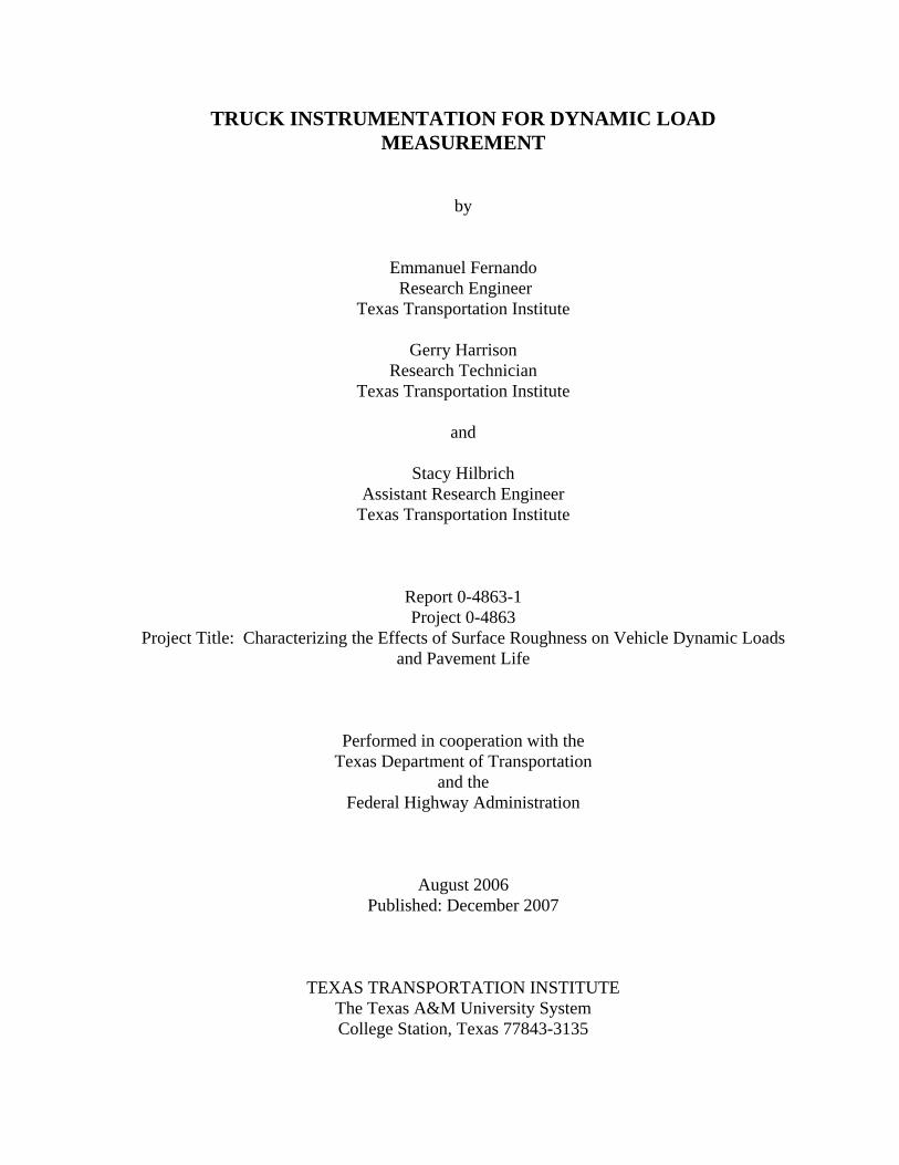
To verify the application of shear strain gages for load measurement, researchers

instrumented a steel bar of rectangular cross-section with a pair of two-element 90° strain

rosettes. Figure 2.3 illustrates the strain rosette used for this laboratory experiment. Two

such gages were mounted on opposite faces of the rectangular steel bar in a four-arm active

or full bridge configuration. The steel bar was then clamped to a work bench as shown in

Figure 2.4 and used to measure a known set of weights suspended at the free end of the bar.

Researchers note that the bridge was zeroed prior to placing the circular disks of known

weights at the free end of the bar (see Figure 2.4). This action removes the initial strain due

to the weight of the bar and the weight of the disk holder.

The test setup included a signal conditioner, data acquisition module, and a notebook

computer. The strain rosettes were wired to the signal conditioner, which provided the

excitation voltage for the test, amplified the signal from the strain gages, and measured the

voltage change as the bar was loaded. Data from the signal conditioner were fed to the data

acquisition module, which in turn was connected to the notebook computer via a universal

serial bus (USB) cable. A data acquisition program running on the notebook computer

collected and recorded voltage readings during the test. From these measurements,

researchers computed a shear strain of about 8 µε.

9

Figure 2.3. Shear Strain Gage Used for Tests.

10

Figure 2.4. Shear Beam Load Cell Experimental Setup.

Given the Young’s modulus Emod for the bar of 29,000 ksi, researchers computed the

corresponding shear modulus from the equation:

G E=

+mod

( )2 1 ν (2.12)

This calculation gave a shear modulus of 11,284 ksi for a Poisson’s ratio ν of 0.285 for the

steel bar. Since the cross-sectional area (b × h) of the bar is 1 inch2, the total weight of the

circular disks at the free end was computed to be 60.2 lb from Eq. (2.11). This value

compares very closely with the reference weight of 60 lb placed on the bar. The close

agreement verifies the correct application of the strain gage principles in this laboratory

experiment.

SMALL-SCALE TESTING WITH AN INSTRUMENTED TRAILER

Following up on the laboratory test with the shear beam load cell, researchers

instrumented a small trailer with shear strain gages to verify the intended method of

11

measuring dynamic loads. Considering the high cost of renting, instrumenting, and

calibrating an 18-wheeler for the tests planned in this project, researchers believed that a

small-scale experiment to verify the intended method of dynamic load measurement was a

prudent step to take. For this experiment, researchers instrumented the single-axle trailer

shown in Figure 2.5. For this instrumentation, researchers instrumented the left side of the

trailer axle with a pair of two-element 90° strain rosettes (Figure 2.3) of the same make and

model used in the shear beam load cell experiment. This gage is made of Constantan alloy

that is self-temperature compensated for tests on cast iron and steel materials. As shown in

Figure 2.3, the sensor has two grids arranged in a chevron pattern that sense normal strains in

perpendicular directions. The grids have a common connection for use in half-bridge circuits,

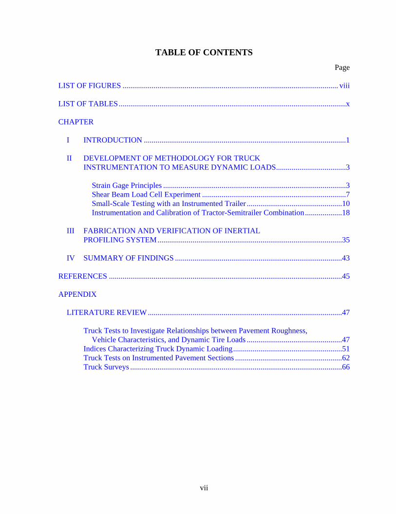
which yield the shear strain directly. Two such gages were mounted on the left side of the

trailer axle on opposite faces and were connected to a signal conditioner in a full bridge

configuration. The gages were mounted between the leaf-spring suspension and the inside of

the left tire as shown in Figure 2.6. The installation procedure included the following steps:

Figure 2.5. Small-Scale Trailer Used to Verify Strain Measurement Methodology.

12

Figure 2.6. Strain Gages Positioned between Suspension and Tire of Small Trailer.

• Removed paint from the axle by sanding down to the metal;

• Cleaned sanded area with a light acid solution to remove oil and contamination.

Rinsed with an acid neutralizer solution;

• Positioned the gages on the axle where measurements were to be made and held

temporarily in place with Mylar tape;

• Pulled back the Mylar tape and applied a small amount of AE-10 glue on the axle.

Slowly replaced Mylar tape with the gages onto the axle, carefully squeezing out the

glue so as to get a thin film of the adhesive between the gages and the axle surface;

• Placed the release film, pressure pad, and clamping plate on top of the gages. Held

these items firmly in place with a cable tie long enough to go around the axle. Let the

glue cure for at least 24 hours; and

• Upon curing, removed the clamping plate, pressure pad, release film, and Mylar tape.

Protected the strain gages from road debris during testing by applying a small amount

of silicone sealant on top of the gages.

13

In addition to the strain gages, researchers included two other sensors in the data

acquisition system for field testing. One was a distance encoder that researchers attached to

the left wheel hub of the towing vehicle to tie the strain measurements to ground distance.

The other was a start sensor to locate the start of the section to be tested with the

instrumented trailer.

Researchers determined the load calibration curve for the strain gages mounted to the

trailer using an MTS loading system. For this laboratory calibration, the loading ram of the

MTS was used to apply load at the middle of the axle, as illustrated in Figure 2.5. As loads

were applied, corresponding strains were determined from the voltage readings measured

with the signal conditioner and recorded with the data acquisition software. These voltage

readings were converted to strains using Eq. (2.7) with Sg = 2.065 and V = 10 volts. In

addition, the force underneath each tire was determined with a load cell positioned under the

tire, as illustrated in Figure 2.7. From these load and strain measurements, researchers

determined the load calibration curve given in Figure 2.8. As observed, the load-strain

relationship is linear over the range of loads at which the trailer was tested, and the

regression line fits the data points quite well. This linear relationship is given by the

equation:

Left tire load (lb) = -18.9 – 15.1 × shear strain (µε) (2.13)

The above equation has a coefficient of determination (R2) of 99.5 percent and a standard

error of the estimate (SEE) of 22.7 lb.

After the laboratory calibration, researchers collected data with the trailer on a weigh-

in-motion (WIM) site located along SH6 close to the intersection with FM60 in College

Station. Figures 2.9 to 2.13 plot the dynamic tire loads determined from the left strain gage

readings collected from five runs made with the instrumented trailer. Also shown is the

WIM measurement for each run. Researchers note the following observations from these

charts:

14

Figure 2.7. Load Cell Placed under Tire during Calibration of Small Trailer.

Figure 2.8. Data from Laboratory Calibration of Small Trailer.

15

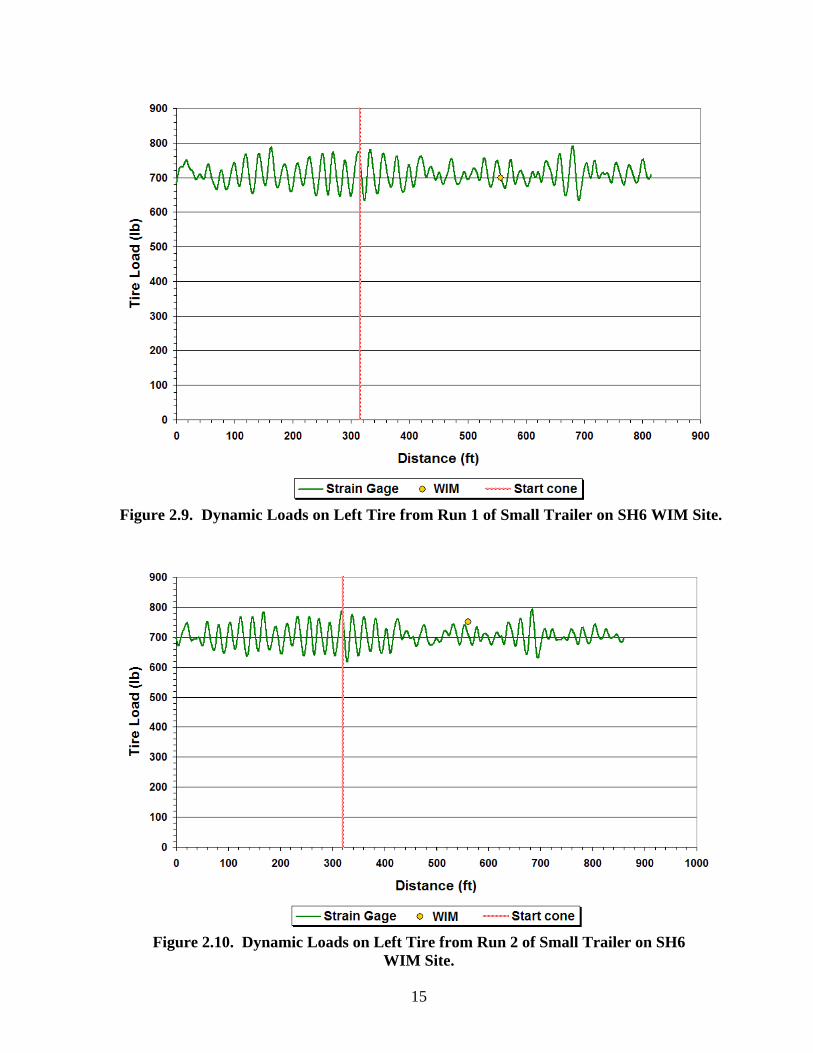
Figure 2.9. Dynamic Loads on Left Tire from Run 1 of Small Trailer on SH6 WIM Site.

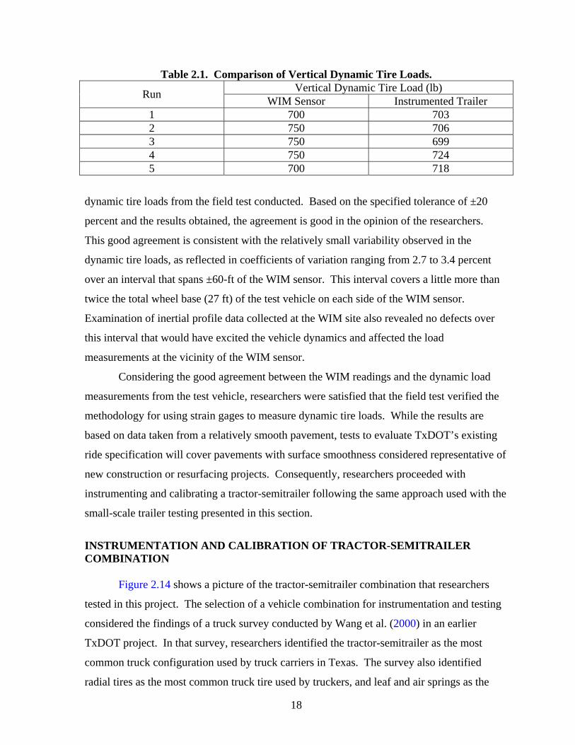
Figure 2.10. Dynamic Loads on Left Tire from Run 2 of Small Trailer on SH6

WIM Site.

16


WIM Site.


WIM Site.

17


WIM Site.

• The dynamic tire loads vary closely about the static tire load of 700 lb,

• The dynamic tire loads determined around the vicinity of the WIM sensor are in

reasonable agreement with the corresponding WIM measurement on each of the five

runs, and

• The load measurements show similar patterns between repeat runs.

Table 2.1 compares the WIM readings with the corresponding dynamic tire loads determined

from the strain gages. A statistical test of the difference between the means indicated no

significant difference (at the 5 percent level) between the averages of the WIM readings and

the dynamic loads determined from the strain gages. With respect to the static tire load of

700 lb, the WIM sensor readings varied from zero to about 7 percent of the static load on the

runs made. For the instrumented trailer, the percent difference ranged from about zero to

3 percent. Researchers note that the American Society for Testing and Materials (ASTM)

stipulates a requirement of ±20 percent on wheel load measurements for Type III WIM

systems in its ASTM E-1318 specification. The results presented should not be interpreted to

mean that the WIM system classifies as a Type III. Rather, the specification is simply given

to provide a reference with which to judge the level of agreement between the static and

18

Table 2.1. Comparison of Vertical Dynamic Tire Loads. Vertical Dynamic Tire Load (lb) Run WIM Sensor Instrumented Trailer

1 700 703 2 750 706 3 750 699 4 750 724 5 700 718

dynamic tire loads from the field test conducted. Based on the specified tolerance of ±20

percent and the results obtained, the agreement is good in the opinion of the researchers.

This good agreement is consistent with the relatively small variability observed in the

dynamic tire loads, as reflected in coefficients of variation ranging from 2.7 to 3.4 percent

over an interval that spans ±60-ft of the WIM sensor. This interval covers a little more than

twice the total wheel base (27 ft) of the test vehicle on each side of the WIM sensor.

Examination of inertial profile data collected at the WIM site also revealed no defects over

this interval that would have excited the vehicle dynamics and affected the load

measurements at the vicinity of the WIM sensor.

Considering the good agreement between the WIM readings and the dynamic load

measurements from the test vehicle, researchers were satisfied that the field test verified the

methodology for using strain gages to measure dynamic tire loads. While the results are

based on data taken from a relatively smooth pavement, tests to evaluate TxDOT’s existing

ride specification will cover pavements with surface smoothness considered representative of

new construction or resurfacing projects. Consequently, researchers proceeded with

instrumenting and calibrating a tractor-semitrailer following the same approach used with the

small-scale trailer testing presented in this section.

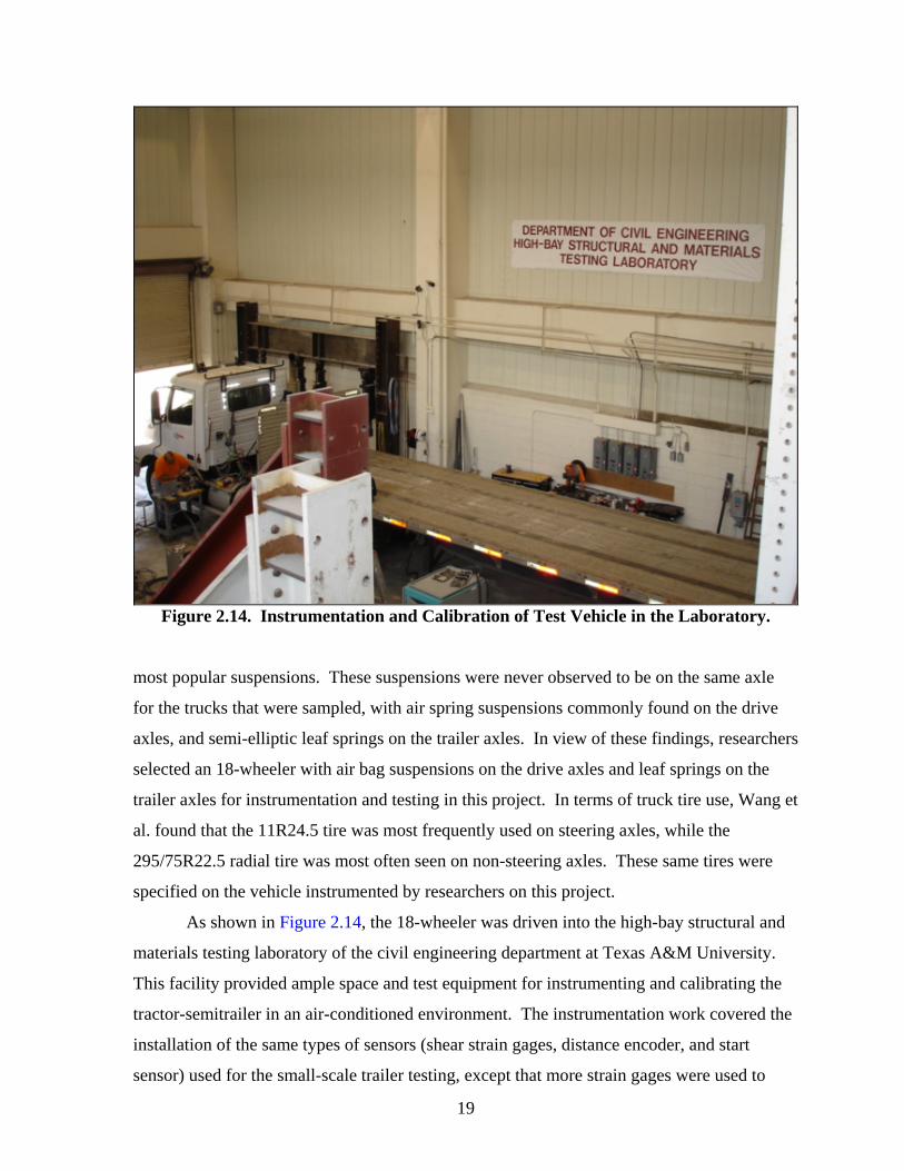
INSTRUMENTATION AND CALIBRATION OF TRACTOR-SEMITRAILER COMBINATION Figure 2.14 shows a picture of the tractor-semitrailer combination that researchers

tested in this project. The selection of a vehicle combination for instrumentation and testing

considered the findings of a truck survey conducted by Wang et al. (2000) in an earlier

TxDOT project. In that survey, researchers identified the tractor-semitrailer as the most

common truck configuration used by truck carriers in Texas. The survey also identified

radial tires as the most common truck tire used by truckers, and leaf and air springs as the

19

Figure 2.14. Instrumentation and Calibration of Test Vehicle in the Laboratory.

most popular suspensions. These suspensions were never observed to be on the same axle

for the trucks that were sampled, with air spring suspensions commonly found on the drive

axles, and semi-elliptic leaf springs on the trailer axles. In view of these findings, researchers

selected an 18-wheeler with air bag suspensions on the drive axles and leaf springs on the

trailer axles for instrumentation and testing in this project. In terms of truck tire use, Wang et

al. found that the 11R24.5 tire was most frequently used on steering axles, while the

295/75R22.5 radial tire was most often seen on non-steering axles. These same tires were

specified on the vehicle instrumented by researchers on this project.

As shown in Figure 2.14, the 18-wheeler was driven into the high-bay structural and

materials testing laboratory of the civil engineering department at Texas A&M University.

This facility provided ample space and test equipment for instrumenting and calibrating the

tractor-semitrailer in an air-conditioned environment. The instrumentation work covered the

installation of the same types of sensors (shear strain gages, distance encoder, and start

sensor) used for the small-scale trailer testing, except that more strain gages were used to

20

permit measurement of tire loads for all five axles of the tractor-semitrailer. Additionally,

researchers added thermocouple sensors to monitor temperatures at the steering, drive, and

trailer axle assemblies during testing. Researchers note that temperature sensitivity of the

strain measurements is not considered to be an issue in view of the temperature-compensated

strain gages and the full bridge configuration used in the truck instrumentation. Nevertheless,

researchers decided to add thermocouples for monitoring test temperatures, which might later

prove useful for data analysis and interpretation.

Figure 2.15 shows the layout of the sensors, signal conditioning, and data acquisition

devices on the test vehicle. All strain gages were wired to the same signal conditioner used

in the small-scale trailer testing. This conditioner amplified the gage readings and measured

the voltage changes in all strain gage channels during testing. Data from all channels

(including the distance encoder, start sensor, and thermocouples) fed into a 16-bit Model

9834 Data Translation module with a 500 KHz maximum sampling rate. This module was

connected to a notebook computer for data collection via a USB cable. A general purpose

data acquisition program was used to read and record data from all channels during testing.

Researchers specified a sampling rate of 4 KHz for each channel on test runs made to collect

dynamic load measurements on in-service pavement sections.

Figure 2.15. Layout of Sensors, Signal Conditioning, and Data Acquisition Devices on

Instrumented Truck.

21

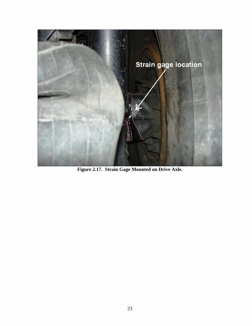
Similar to the installation of strain gages for the small-scale trailer testing, the gages

were mounted on the 18-wheeler between the suspension and inside tire of each axle as

illustrated in Figures 2.16 and 2.17. Two shear strain gages were mounted on each side of

the axle on opposite faces, one toward the front and the other toward the rear of the test

vehicle. Each strain gage pair was wired in a full bridge configuration for dynamic load

measurement on that side of the given axle.

After installation of the gages and set up of the data acquisition system, researchers

conducted calibrations to determine the load-strain relationships for the different gages. This

calibration was conducted in a similar manner as the small trailer calibration except that more

axles were tested, beginning with the trailer tandem axle, then the drive, and finally the

steering axle. For calibrating each axle group, researchers positioned a loading plate

(Figure 2.18) on the trailer flatbed at the geometric center of the tandem axle assembly where

gages were to be calibrated. In this way, the applied vertical loads to the loading plate were

distributed primarily to the axle group that was being calibrated. To measure the vertical tire

loads during calibration, technicians used the loading crane of the high-bay laboratory to lift

the axle assembly and position load cells underneath each dual tire (Figure 2.19).

Researchers then recorded the readings from the strain gages on the axle group along with

the corresponding vertical tire loads from the load cells during calibration.

Prior to calibrating the strain gages, researchers calibrated the load cells by

determining the relationship between the readings from each load cell and the corresponding

loads measured with the reference load cell maintained by the high-bay structural and

materials testing laboratory. The authors note that the calibration of the reference load cell is

National Institute of Standards and Technology (NIST) traceable. During calibration, the

voltage readings from the test load cells were recorded along with the corresponding load

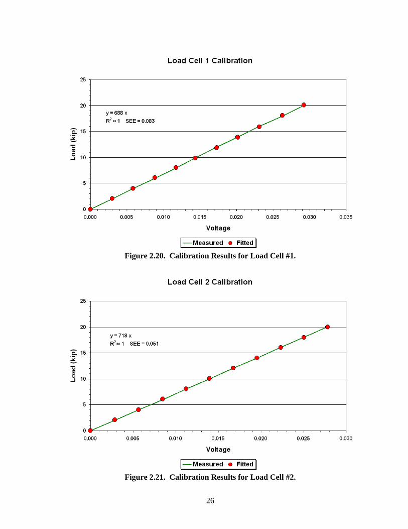
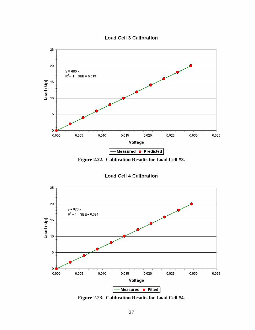
magnitudes measured with the reference load cell. Figures 2.20 to 2.23 show the calibration

equations determined from these tests. The relationships show a high degree of linearity over

the range of loads at which the calibrations were conducted. In addition, the regression line

fits the test data for each load cell very well. Thus, researchers used the relationships shown

to calibrate the strain gages mounted on the tractor-semitrailer for measurement of dynamic

tire loads.

During calibration, researchers used a 100-kip MTS system to apply loads to the axle

assembly through the loading plate positioned at the geometric center of the axle assembly

22

Figure 2.16. Strain Gage Mounted on Trailer Axle.

23

Figure 2.17. Strain Gage Mounted on Drive Axle.

24

Figure 2.18. Application of Load to Axle Assembly through Loading Plate.

(axle assembly underneath the loading plate and load ram)

25

Figure 2.19. Load Cells Positioned under Dual Tires of Trailer Axle Assembly.

26

Figure 2.20. Calibration Results for Load Cell #1.


27



28

where gages were to be calibrated. The first step in the calibration was to zero the strain

gages and load cells. This step was accomplished with the axle assembly raised above

ground using the loading crane. After zeroing the strain gages and load cells, technicians

carefully lowered the axle assembly back onto the load cells. The initial strain and load cell

readings were then recorded with no other loads applied to the trailer. Subsequently,

researchers applied a series of loads to the axle group using the 100-kip MTS system. At

each load level, strain gage and load cell readings were recorded to collect data for

determining the calibration curves of the different gages mounted on the axle assembly tested.

This loading sequence was followed by an unloading sequence during which readings were

taken as the loads were reduced.

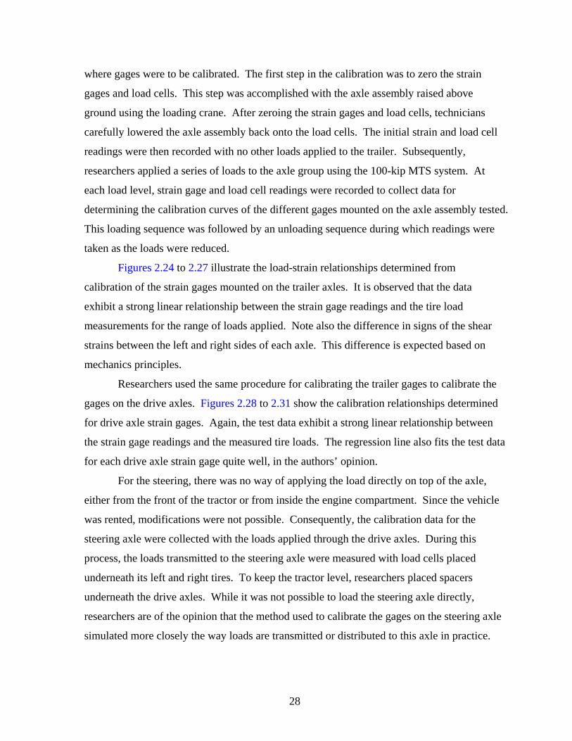
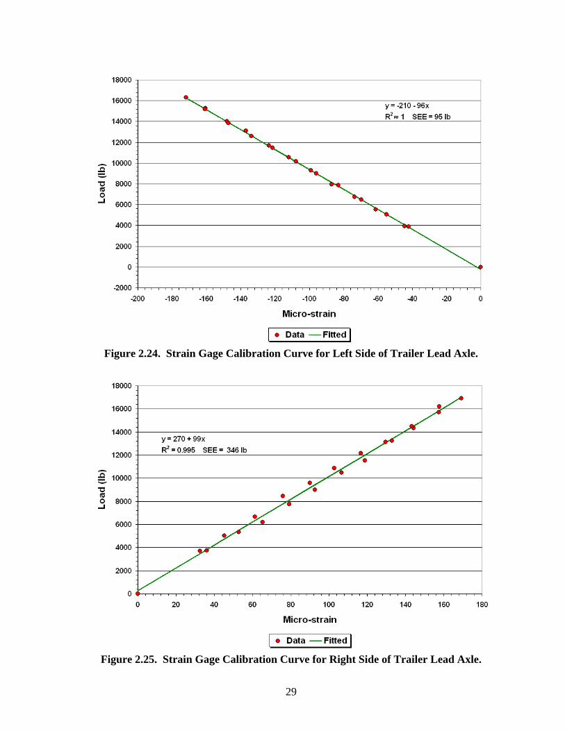
Figures 2.24 to 2.27 illustrate the load-strain relationships determined from

calibration of the strain gages mounted on the trailer axles. It is observed that the data

exhibit a strong linear relationship between the strain gage readings and the tire load

measurements for the range of loads applied. Note also the difference in signs of the shear

strains between the left and right sides of each axle. This difference is expected based on

mechanics principles.

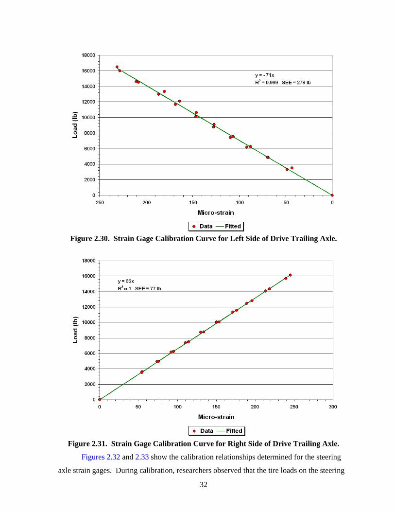
Researchers used the same procedure for calibrating the trailer gages to calibrate the

gages on the drive axles. Figures 2.28 to 2.31 show the calibration relationships determined

for drive axle strain gages. Again, the test data exhibit a strong linear relationship between

the strain gage readings and the measured tire loads. The regression line also fits the test data

for each drive axle strain gage quite well, in the authors’ opinion.

For the steering, there was no way of applying the load directly on top of the axle,

either from the front of the tractor or from inside the engine compartment. Since the vehicle

was rented, modifications were not possible. Consequently, the calibration data for the

steering axle were collected with the loads applied through the drive axles. During this

process, the loads transmitted to the steering axle were measured with load cells placed

underneath its left and right tires. To keep the tractor level, researchers placed spacers

underneath the drive axles. While it was not possible to load the steering axle directly,

researchers are of the opinion that the method used to calibrate the gages on the steering axle

simulated more closely the way loads are transmitted or distributed to this axle in practice.

29

Figure 2.24. Strain Gage Calibration Curve for Left Side of Trailer Lead Axle.

Figure 2.25. Strain Gage Calibration Curve for Right Side of Trailer Lead Axle.

30

Figure 2.26. Strain Gage Calibration Curve for Left Side of Second Trailer Axle.

Figure 2.27. Strain Gage Calibration Curve for Right Side of Second Trailer Axle.

31

Figure 2.28. Strain Gage Calibration Curve for Left Side of Drive Lead Axle.

Figure 2.29. Strain Gage Calibration Curve for Right Side of Drive Lead Axle.

32

Figure 2.30. Strain Gage Calibration Curve for Left Side of Drive Trailing Axle.

Figure 2.31. Strain Gage Calibration Curve for Right Side of Drive Trailing Axle.

Figures 2.32 and 2.33 show the calibration relationships determined for the steering

axle strain gages. During calibration, researchers observed that the tire loads on the steering

33

axle did not vary appreciably with changes in the load applied through the drive axle

assembly, as may be inferred from the range of tire loads plotted in Figures 2.32 and 2.33.

This observation is consistent with weigh-in-motion data on five axle tractor-semitrailer

combination trucks where the most consistent axle weight is from the steer axles, which

remains reasonably constant under various loading scenarios.

Figure 2.32. Strain Gage Calibration Curve for Left Side of Steering Axle.

34

Figure 2.33. Strain Gage Calibration Curve for Right Side of Steering Axle.

35

CHAPTER III. FABRICATION AND VERIFICATION OF INERTIAL PROFILING SYSTEM

Profile measurements are needed to evaluate relationships between vehicle dynamic

loads and surface roughness for the purpose of evaluating the current ride specification in this

project. Initially, researchers instrumented a tractor-semitrailer with a portable inertial

profiling system to permit synchronized collection of dynamic tire loads and surface profiles

during testing. However, tests to verify profiler performance based on the certification

requirements in TxDOT Test Method Tex-1001S were not successful. Compared to the

vibrations from vans or light trucks on which profilers are commonly used, the vibrations

from the test vehicle were considerably larger, resulting in failure of the dampeners used to

isolate the accelerometers and lasers of the profiling system from vibrations of the test

vehicle during testing. The dampeners sheared off after several repeat runs of the test truck

on the pavement sections used to evaluate the on-board inertial profiling system.

Following the suggestion of the project monitoring committee, researchers dropped

the idea of instrumenting a tractor-semitrailer with an inertial profiling system. Instead of

this approach, profile data were to be collected using a high-speed inertial profiler separate

from the instrumented vehicle combination. To minimize differences between wheel paths

tracked, the sensors of the inertial profiler would be set to match the spacing between the

dual wheels on the left and right sides of the instrumented tractor-semitrailer. In addition, the

operator of the inertial profiler would try to take data as close as possible on the same wheel

paths where dynamic load measurements were collected with the instrumented truck.

Ordinarily, this project would have used one of TxDOT’s inertial profilers to collect

profile measurements. However, problems with the availability of an inertial profiler led

researchers to instrument a test vehicle with an inertial profiling system to conduct the

required tests. This instrumentation was an in-house effort funded by TTI. The profiling

system followed the same design developed by Walker (1997) and used existing software.

The main components of the profiler are:

• a chassis unit containing the power supply and signal interface modules,

• two laser/accelerometer modules mounted on the front of the test vehicle,

• a Model 9803 Data Translation board for data acquisition,

• a distance encoder,

36

• a start sensor, and

• a notebook computer.

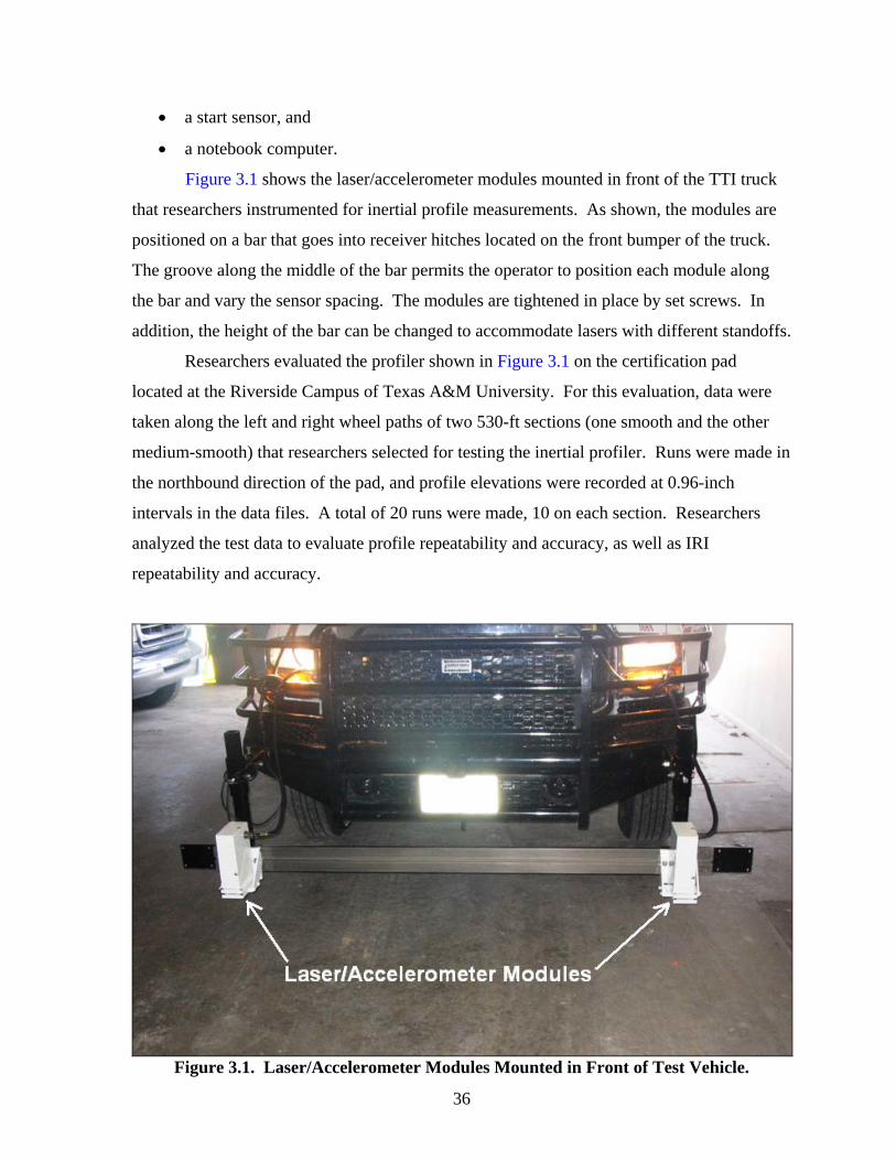
Figure 3.1 shows the laser/accelerometer modules mounted in front of the TTI truck

that researchers instrumented for inertial profile measurements. As shown, the modules are

positioned on a bar that goes into receiver hitches located on the front bumper of the truck.

The groove along the middle of the bar permits the operator to position each module along

the bar and vary the sensor spacing. The modules are tightened in place by set screws. In

addition, the height of the bar can be changed to accommodate lasers with different standoffs.

Researchers evaluated the profiler shown in Figure 3.1 on the certification pad

located at the Riverside Campus of Texas A&M University. For this evaluation, data were

taken along the left and right wheel paths of two 530-ft sections (one smooth and the other

medium-smooth) that researchers selected for testing the inertial profiler. Runs were made in

the northbound direction of the pad, and profile elevations were recorded at 0.96-inch

intervals in the data files. A total of 20 runs were made, 10 on each section. Researchers

analyzed the test data to evaluate profile repeatability and accuracy, as well as IRI

repeatability and accuracy.

Figure 3.1. Laser/Accelerometer Modules Mounted in Front of Test Vehicle.

37

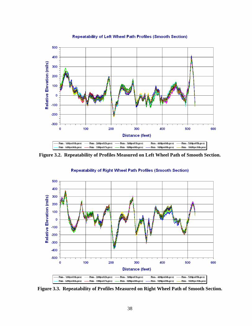
Figures 3.2 to 3.5 illustrate the repeatability of the profiles measured on each section.

Tables 3.1 to 3.4 summarize the statistics determined from the analysis of test data. The

results presented show that the profiler (as configured) meets the requirements for inertial

profiler certification stipulated in TxDOT Test Method Tex-1001S and that a suitable

profiling system has been built for use on this project as well as on other research projects

where this capability is needed.

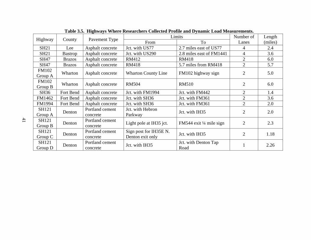
Having successfully fabricated an inertial profiler, researchers collected profile data

on a number of TxDOT paving projects to evaluate the Department’s current Item 585 ride

specification. Table 3.5 identifies the projects tested. All projects, with the exception of

SH47 in Brazos County, were completed within 3 months of the profile surveys done in this

research project. SH47 is an existing highway that is not a newly resurfaced project.

Researchers included SH47 on the routes that were surveyed because of the smooth ride

scores reported on this highway in TxDOT’s pavement management information system

database. On the same projects identified in Table 3.5, researchers collected dynamic tire

load data using the instrumented tractor-semitrailer combination described in Chapter II of

this interim report. Researchers then analyzed these measurements in conjunction with the

profile data collected on these projects to evaluate TxDOT’s Item 585 ride specification. The

reader is referred to the final project report by Fernando, Harrison, and Hilbrich (2007) for

the details of this evaluation.

38

Figure 3.2. Repeatability of Profiles Measured on Left Wheel Path of Smooth Section.

Figure 3.3. Repeatability of Profiles Measured on Right Wheel Path of Smooth Section.

39

Figure 3.4. Repeatability of Profiles Measured on Left Wheel Path of

Medium Smooth Section.

Figure 3.5. Repeatability of Profiles Measured on Right Wheel Path of

Medium Smooth Section.

40

Table 3.1. Repeatability of Profile Measurements from TTI Profiler. Test Section Wheel Path Average Standard Deviation (mils)1

Left 16 Smooth

Right 17

Left 18 Medium-Smooth

Right 21 1 Not to exceed 35 mils per TxDOT Test Method Tex-1001S

Table 3.2. Repeatability of IRIs from Profile Measurements with TTI Profiler. Test Section Wheel Path Standard Deviation (inches/mile)1

Left 0.89 Smooth

Right 0.74

Left 1.10 Medium-Smooth

Right 0.54 1 Not to exceed 3.0 inches/mile per TxDOT Test Method Tex-1001S

Table 3.3. Accuracy of Profile Measurements from TTI Profiler.

Test Section Wheel Path Average Difference (mils)1 Average Absolute Difference (mils)2

Left -1 11 Smooth

Right 0 11

Left 2 13 Medium-Smooth

Right 3 13 1 Must be within ±20 mils per TxDOT Test Method Tex-1001S 2 Not to exceed 60 mils per TxDOT Test Method Tex-1001S

Table 3.4. Accuracy of IRIs from Profile Measurements with TTI Profiler. Test Section Wheel Path Difference (inches/mile)1

Left 0.12 Smooth

Right 0.94

Left 0.04 Medium-Smooth

Right -1.19 1 Absolute difference not to exceed 12 inches/mile per TxDOT Test Method Tex-1001S

41

Table 3.5. Highways Where Researchers Collected Profile and Dynamic Load Measurements. Limits Highway County Pavement Type From To

Number of Lanes

Length (miles)

SH21 Lee Asphalt concrete Jct. with US77 2.7 miles east of US77 4 2.4 SH21 Bastrop Asphalt concrete Jct. with US290 2.8 miles east of FM1441 4 3.6 SH47 Brazos Asphalt concrete RM412 RM418 2 6.0 SH47 Brazos Asphalt concrete RM418 5.7 miles from RM418 2 5.7

FM102 Group A Wharton Asphalt concrete Wharton County Line FM102 highway sign 2 5.0

FM102 Group B Wharton Asphalt concrete RM504 RM510 2 6.0

SH36 Fort Bend Asphalt concrete Jct. with FM1994 Jct. with FM442 2 1.4 FM1462 Fort Bend Asphalt concrete Jct. with SH36 Jct. with FM361 2 3.6 FM1994 Fort Bend Asphalt concrete Jct. with SH36 Jct. with FM361 2 2.0 SH121

Group A Denton Portland cement concrete

Jct. with Hebron Parkway Jct. with IH35 2 2.0

SH121 Group B Denton Portland cement

concrete Light pole at IH35 jct. FM544 exit ¼ mile sign 2 2.3

SH121 Group C Denton Portland cement

concrete Sign post for IH35E N. Denton exit only Jct. with IH35 2 1.18

SH121 Group D Denton Portland cement

concrete Jct. with IH35 Jct. with Denton Tap Road 1 2.26

43

CHAPTER IV. SUMMARY OF FINDINGS

This interim report documented the research efforts conducted in this project to

provide an instrumented tractor-semitrailer combination for measurement of dynamic loads,

and a high-speed inertial profiler for measurement of surface profiles. These capabilities are

needed to collect data with which to evaluate TxDOT’s Item 585 smoothness specification

for the purpose of verifying whether it permits certain profile wavelengths to pass that are

detrimental to pavement life based on dynamic loading criteria. Based on the experience

with the instrumentation efforts, the authors note the following findings:

• The application of strain gages for load measurement was successfully demonstrated

in a laboratory setting with a shear beam load cell experiment wherein a steel bar,

instrumented with shear strain gages in a full bridge configuration, was used to

measure the total weight of a known set of circular disks. The shear beam load cell

gave a measurement within 0.33 percent of the known total weight of the circular

disks.

• Small-scale testing with an instrumented trailer verified the method for positioning,

mounting, wiring, and calibrating the strain gages on the test vehicle. From the

results of the trailer calibration, researchers observed a strong linear relationship

between tire load and strain over the range of loads at which the calibration was

conducted. In addition, results of tests on a weigh-in-motion site showed that:

the dynamic tire loads determined from the strain gages vary closely about the

measured static tire load of 700 lb,

the dynamic tire loads determined around the vicinity of the WIM sensor are

in reasonable agreement with the corresponding WIM measurement on each

repeat run, and

the load measurements exhibit similar patterns between repeat runs.

In view of the positive results, researchers proceeded with instrumenting and

calibrating a tractor-semitrailer combination following the same approach used for

the small-scale trailer tests.

• The calibration curves from full-scale laboratory tests of the instrumented tractor-

semitrailer exhibit a strong linear relationship between tire load and shear strain. The

44

shear strains measured between the left and right sides of a given axle also show a

difference in signs, as expected from theory.

• Researchers also instrumented a test vehicle with an inertial profiling system and

verified its performance based on TxDOT Test Method Tex-1001S. The results

obtained show that the profiler meets the certification requirements specified in the

test method.

45

REFERENCES Addis, R. R., A. R. Halliday, and C. G. B. Mitchell. Dynamic Loading of Road Pavements by Heavy Goods Vehicles. Congress on Engineering Design, Seminar 4A-03, Birmingham, Institution of Mechanical Engineers, 1986. Chatti, K., and D. Lee. Development of New Profile-Based Truck Dynamic Load Index. Transportation Research Record 1806, Transportation Research Board, Washington, D.C., 2002, pp. 149-159. Dally, J. W., and W. F. Riley. Experimental Stress Analysis. 2nd edition, McGraw-Hill, Inc., N.Y., 1978. Fernando, E. G., G. Harrison, and S. Hilbrich. Evaluation of Ride Specification Based on Dynamic Load Measurements from Instrumented Truck. Technical Report 0-4863-2, Texas Transportation Institute, Texas A&M University, College Station, Tex., 2007. Fernando, E. G. Index for Evaluating Initial Overlay Smoothness with Measured Profiles. Transportation Research Record 1806, Transportation Research Board, Washington, D.C., 2002, pp. 121-130. Fernando, E. G., and C. Bertrand. Application of Profile Data to Detect Localized Roughness. Transportation Research Record 1813, Transportation Research Board, Washington, D.C., 2002, pp. 55-61. Fernando, E. G. Development of a Profile-Based Smoothness Specification for Asphalt Concrete Overlays. Research Report 1378-S, Texas Transportation Institute, Texas A&M University, College Station, Tex., 1998. Gyenes, L., and C. G. B. Mitchell. Measuring Dynamic Loads for Heavy Vehicle Suspensions Using a Road Simulator. International Journal of Heavy Vehicle Systems, Vol. 3, 1996. Hassan, R. A., and K. McManus. Assesssment of Interaction Between Road Roughness and Heavy Vehicles. Transportation Research Record 1819, Transportation Research Board, Washington, D.C., 2003, pp. 236-243. Huhtala, M., V. Laitinen, and P. Halonen. Roughness Measurement Devices and Dynamic Truck Index. International Conference on the Bearing Capacity of Roads and Airfields, Minneapolis, Minn., 1994, pp. 1517-1531. Jacob, B., and V. Dolcemascolo. Dynamic Interactions Between Instrumented Vehicles and Pavements. International Symposium on Heavy Vehicle Weights and Dimensions, Queensland, Australia, 1998, pp. 142-160.

46

Merril, D. B., D. Blackman, and V. Ramdas. The Implications of Dynamic Loading and Tire Type on the UK Road Network. International Conference on Asphalt Pavements, Copenhagen, Denmark, 2002. Middleton, J., and A. H. Rhodes. The Effect of Dynamic Loading on Road Pavement Wear: A Study of the Relationship Between Road Profiles and Pavement Wear on an Instrumented Test Road. Proceedings of the Institution of Civil Engineers, Vol. 105, 1994. Papagiannakis, T., and B. Raveendran. International Standards Organization – Compatible Index for Pavement Roughness. Transportation Research Record 1643, Transportation Research Board, Washington, D.C., 1998, pp. 110-115. Roberts, F. L., J. T. Tielking, D. Middleton, R. L. Lytton, and K. Tseng. Effects of Tire Pressures on Flexible Pavements. Research Report 372-1F, Texas Transportation Institute, Texas A&M University, College Station, Tex., 1986. Steven, B., and J. de Pont. Dynamic Loading Effects on Pavement Performance – The OECD Divine Test at CAPTIF. ARRB Transport Research Conference, Christchurch, New Zealand, 1998, pp. 93-107. University of Michigan Transportation Research Institute (UMTRI). RoadRuf User Reference Manual, The University of Michigan, Ann Arbor, Mich., 1997. Walker, R. S. Real-Time Data Acquisition for Surface Measurement/Implementation of Intelligent Bus Systems for Distress Measurements. Research Report 19987-F, The University of Texas at Arlington, Arlington, Tex., 1997. Wang, F., and R. B. Machemehl. Current Status and Variability of In-Service Truck Tire Pressures in Texas. Transportation Research Record 1853, Transportation Research Board, Washington, D.C., 2003, pp. 157-164. Wang, F., R. F. Inman, R. B. Machemehl, Z. Zhang, and C. M. Walton. Study of Current Truck Configurations. CTR Report 0-1862-1, Center for Transportation Research, The University of Texas at Austin, Austin, Tex., 2000.

47

APPENDIX LITERATURE REVIEW

Researchers conducted a literature review to gather information considered useful for

accomplishing the objectives of this project. The review covered the following areas:

• measurement of vehicle dynamic loads,

• surveys of truck use that identified configurations commonly used by carriers to

transport goods and commodities,

• profile statistics for characterizing pavement smoothness based on truck damage

criteria,

• vehicle transfer functions relating pavement roughness to dynamic tire loading, and

• compilations of data on truck properties for simulating the response of trucks to

pavement roughness.

The findings from the literature review are presented in this appendix.

TRUCK TESTS TO INVESTIGATE RELATIONSHIPS BETWEEN PAVEMENT ROUGHNESS, VEHICLE CHARACTERISTICS, AND DYNAMIC TIRE LOADS

In a 1996 report, Gyenes and Mitchell detail research conducted at Transport Research

Laboratories (TRL) in the United Kingdom (UK), in which the Volvo test facility in

Gothenburg was utilized to develop a simulated test to rate suspensions in terms of their

potential for causing road wear. This goal was accomplished by comparing simulated wheel

load measurements published by TRL in 1993 to actual dynamic behavior of heavy goods

vehicle suspensions over the TRL test track. The first test series in 1991 involved a

computer-controlled Volvo rig made up of six hydraulic actuators capable of exercising a

fully laden vehicle. The TRL test track profiles were run through the actuators, and a

comparison was made between the Volvo instrumentation, which measured the dynamic

loads under the tire patch using load cells built into the actuators, and the TRL

instrumentation, which used strain gages and accelerometers. In addition, researchers

compared rig generated wheel load histories against real road-based load histories from the

TRL test track program.

A second test series was conducted in 1993 to obtain the unsprung masses by the

process of dynamic calibration, followed by systematic runs at simulated test speeds of 20,

48

30, 40, 50, and 60 mph using the smooth and medium-smooth wheel track profiles of the

TRL test track as inputs. The suspensions for the two-axle semitrailer bogies used for testing

included a tandem axle air suspension; a tandem axle, single-leaf steel suspension; and a

rubber mounted walking beam suspension. The vehicles were fully loaded to the UK gross

vehicle weight limit of 32.5 tons with tandem axle weights of about 18 tons on each

semitrailer bogie.

Wheel loads on the road simulator were measured using load cells built into the

actuators close to the wheel platforms. The load on each wheel of the replaceable

sub-chassis unit was determined by measuring the bending of the axle between the spring

mount and the wheel hub using strain gages, and the vertical inertia of the wheel mass using

an accelerometer mounted on the hub back plate. Strain gages fitted to the bogie with the

rubber-mounted walking beam suspension measured the shear force on the axle tube, a

technique that provided higher accuracy in dynamic load measurement compared to bending

gages.

Accelerometers were fitted to the semitrailer platform to measure body bounce, pitch,

and roll accelerations. Displacement transducers were also fitted to each semitrailer wheel to

measure vertical displacement between the axle center and the trailer platform. The

accelerometers and strain gages were calibrated before each test series, and the signals from

the actuator sensors and body-mounted sensors were recorded on the same data logger.

The steel, air, and rubber-suspended tandem axles were sinusoidally excited over a range of

frequencies from 0.5 Hz to 20 Hz in bounce, pitch, roll, and twist modes. The results of the

constant speed excitation in bounce for the nearside rear wheel of all three suspension types

indicate that there are two dominant modes – the body bounce at low frequency and the

wheel hop at high frequency. As the excitation frequency is increased, the effect of the

unsprung mass on wheel loads becomes significant. The results of the constant speed

excitation in pitch for the nearside rear wheel of all three suspension types indicate that there

is one dominant mode, which is at high frequency. The results of the constant speed

excitation in roll for the nearside rear wheel of all three suspension types are evident at

around 1 Hz. The results of the constant speed excitation in twist for the nearside rear wheel

of all three suspension types indicate that there is no distinct mode in the range of excitation

frequencies.

49

The results of these tests showed that the dynamic wheel load can be measured within

1 to 2 percent accuracy when using an improved technique, which involves the use of shear

gages and a dynamic calibration procedure that corrects for the angular and vertical

accelerations of the wheel components outboard of the strain gages. According to the

researchers, this method is an improvement over other methods, which use bending gages

that are subject to anomalous readings of the roll component of wheel load.

Middleton and Rhodes’ 1994 report detail their research, which was based on

previous work conducted by Addis, Halliday, and Mitchell in 1986. In the research

performed by Addis et al., a two-axle, semitrailer was instrumented, and results were

obtained from one vehicle operating over one instrumented pavement. Middleton and

Rhodes decided to further this research and constructed a test laboratory with a more

comprehensive system of strain gages that could be used to monitor the structural effects of

the passage of any vehicle passing over the test section at various speeds. Each strain gage

was calibrated using dynamic wheel loads data from an instrumented two-axle heavy goods

vehicle, which allowed the monitoring of instantaneous dynamic wheel loads of any vehicle

at any point along the test section. The test facility was instrumented with strain gages with

120 ohm resistance-foil located at the bottom of the roadbed to measure the transient

horizontal radial strain at 0.5 m centers under each wheel path. There were a total of 126

strain gages.

The test vehicle used in the study was a Volvo instrumented at TRL. It was

instrumented to permit measurements of all wheel loads simultaneously, using strain gages

that measured the bending of the axles between the suspension and the hub. Accelerometers

were also used to correct the vertical inertial loads due to the unsprung mass outboard of the

strain gages.

The instrumented test vehicle was used to calibrate the strain gages. This was done to

establish the relationship between vehicle speed, transient strain, and the respective dynamic

wheel loads. The calibration data were used so that the instantaneous wheel loads of any

vehicle traveling along the wheel paths could be monitored.

The longitudinal profiles of the two wheel-tracks were monitored regularly using the

TRL high speed road monitor. During testing, a record was kept for temperature, wind

speed, and rainfall in order to ensure that strain measurements were taken under similar

conditions. Wheel paths were surveyed regularly for rutting and cracking. Twelve sets of

50

dynamic wheel load data were collected under a combination of variables, which included

number of axles, speed, and number of wheel paths. A minimum of two sets of pavement

strain data were collected for each strain gage, and thermocouples were used to measure the

pavement temperatures at the surface, at 20 mm depth, and at 250 mm depth at the

beginning, middle, and end of the test section.

The results of this research provided several conclusions. One conclusion was that

the wheels of the test vehicles applied dynamic loading, which oscillated between 3 Hz and

appeared to be independent of speed, load, tire type, and suspension system. Also, the

researchers concluded that each axle of the test vehicles applied maximum and minimum

dynamic loads at common points for a specific speed and that the ratio of mean dynamic axle

load and static axle load increased with speed.

Jacob and Dolcemascolo’s 1998 report details their investigation into dynamic loads

on pavements and their spatial repeatability to assess the sensitivity to pavement profile, road

roughness, vehicle characteristics, and traveling conditions. The investigation also looked

into the effects of dynamic loads on vehicles and the infrastructure and focused on the

response of two instrumented vehicles traveling at the same speeds on different road profiles,

whose evenness were considered excellent, good, and poor. The IRI values in m/km of each

road section were found to be 0.8 for the road in excellent condition, 1.73 for the road in

good condition, and 3.57 for the road in poor condition.

The two vehicles were instrumented with strain gages mounted on the axles and

accelerometers on the bodies, which provide the data to calculate dynamic wheel impact

forces at high frequency. The wheel load instrumentation was made up of two strain gage

bridges and two accelerometers per axle, which were configured as full bridge circuits that

were sensitive to shear force. These instrumented vehicles could measure dynamic wheel

loads with a sampling frequency of 500 Hz.

An instrumented vehicle was also used in this research, which consisted of a two-axle

tractor with a single-axle instrumented trailer that could be equipped with two suspension

types, which were either air or steel leaf spring. This instrumented vehicle could measure

dynamic wheel loads with a sampling frequency of 200 Hz.

For each of the three test sites, the power spectral density (PSD) of the pavement

profile was calculated and plotted versus the wavelength λ. The PSD may be plotted as a

function of frequency ƒ or wavelength because both are linked to the vehicle velocity V

51

according to the relation V= ƒ λ. When plotting the PSD of the pavement profile, the larger

the area under the PSD curve, the greater the roughness.

Two PSDs were calculated for the impact forces of the trailer corresponding to each

combination of the test variables, i.e., test site, suspension, load, and speed. One PSD was

for the axle impact force, which is the sum of both wheel loads and is considered to be

representative of the bounce and axle hop motions. The other PSD was for the difference

between the left and right wheel loads, which is representative of the roll motion. The main

findings were that the body bounce of the steel suspension gives the highest peaks, which

generally increased with pavement roughness. The body bounce peak amplitude is between

10 to 20 times lower with the air suspension than with the steel suspension.

PSDs were also calculated for each wheel and axle load of the instrumented vehicle.

It was found that the shapes of the PSDs for wheel and axle loads are similar for each speed

with the same approximate peaks. The roll effect is more important for wheels, while the

axle hop is higher for axles. The body motions were dominant for the heaviest load, while

the axle hops became the main effect at lower loads with a slight shift in the frequency.

Other significant findings of this research were the importance of wheel imbalance to the

wheel and axle dynamic impact factors (especially at low speed and on smooth road profiles

where the body bounce and axle hop motions are low), the significant reduction in dynamic

load increments from the air suspensions, and the great influence of pavement roughness on

dynamic loads.

INDICES CHARACTERIZING TRUCK DYNAMIC LOADING

The effect of surface profile on vehicle dynamic loads is illustrated in

Figures A1 to A3 (Fernando, 2002). Shown in these figures are the predicted vehicle

responses to measured surface profiles as determined using a vehicle simulation model.

Figure A1 shows the predicted variation in dynamic axle loads on a smooth pavement having

a serviceability index (SI) of 4.5. The plot shown is referred to in this proposal as the

dynamic load profile, analogous to a surface or road profile, which shows the variation in

elevation with distance along a given segment. Figure A2 illustrates the predicted dynamic

load profile for a medium-smooth pavement (SI of 3.4), while Figure A3 shows the load

profile for a rough pavement (SI of 2.5). It is observed from Figures A1 to A3 that the

variability in predicted dynamic axle loads increases with an increase in surface roughness.

52

Figure A1. Predicted Dynamic Loads on a Smooth Pavement (SI = 4.5).

Figure A2. Predicted Dynamic Loads on a Medium-Smooth Pavement (SI = 3.4).

53

Figure A3. Predicted Dynamic Loads on a Rough Pavement (SI = 2.5).

The dynamic axle loads fluctuate about the static axle load, which corresponds to the mean of

the predicted dynamic loadings. In the figures given, the static axle load is 18 kips

corresponding to the standard single axle used in pavement designs currently implemented

within state highway agencies. In the limit, if the surface profile is perfectly flat, the

predicted dynamic loads would be a constant, equal to the static axle load, and the load

profile would plot as a horizontal line. In this case, there will be no variability in the

predicted axle loads. Because pavement response is directly tied to axle load magnitudes, it

is logical to expect that dynamic axle load variations will lead to differences in predicted

pavement performance.

Fernando (2002) proposed an index for evaluating the acceptability of overlay

smoothness that is related to the predicted performance of the overlay based on reflection

crack growth. To illustrate the concept underlying the development of this index, consider

the two pavements shown in Figure A4. In the first case, a smooth overlay is built over the

existing pavement, while in the second case, a rough overlay is constructed. Note that the

underlying pavement is the same for both scenarios, as would be true for a given resurfacing

project. Only the effect of differences in surface profile is considered. From theoretical

considerations, Fernando (1998) developed an index for predicting the change in overlay life

54

Smooth Asphalt Overlay

Rough Asphalt Overlay

Figure A4. Illustration of Approach Used to Evaluate Initial Overlay Smoothness.

55

due to differences between the target and as-built surface profiles. It is given by the equation

0

1

1 11

nz CVz CV

⎡ ⎤+∆ = −⎢ ⎥+⎣ ⎦

(A1)

where

CV0 = coefficient of variation of the applied dynamic wheel loads associated

with the target profile from design,

CV1 = coefficient of variation of the applied dynamic wheel loads associated

with the as-built profile,

z = the number of standard deviations corresponding to a given percentile of

the predicted dynamic load distribution, and

n = the exponent of the Paris-Erdogan crack growth law that affects the rate

of crack propagation through the overlay.

The reader is referred to the report by Fernando (1998) for the derivation of Eq. A1.

This equation provides a rational method for evaluating the quality of the finished surface on

the basis of predicted performance. In practice, the coefficient of variation in Eq. A1 is

determined by vehicle simulation using the measured profile. Note that ∆ is related not only

to the surface profile but to vehicle suspension and geometric characteristics, which all affect

the variability in the applied dynamic wheel loads. The benefit of reducing this variability on

predicted pavement life is readily apparent from Eq. A1. If CV1 < CV0, the predicted index is

positive, indicating a predicted increase in pavement life with a smoother surface. Note that

the reduction in wheel load variability is achieved not only by building smoother pavements

but also by designing, manufacturing, and encouraging the use of trucks with improved

dynamic performance. If the as-built and target profiles are the same, CV0 = CV1 and the

predicted ∆ is zero, indicating that the as-built surface meets the predicted service life

associated with the target smoothness. Finally, if the as-built surface is rougher than the

target, i.e., CV1 > CV0, ∆ is negative, indicating a reduction in predicted pavement life

because of the expected higher impact loading.

Huhtala et al. (1994) reported on the international roughness index developed by the

World Bank in 1982 to classify road surface evenness. The IRI is determined from the

longitudinal profile of the road, which is measured through a variety of methods. The IRI

value of the measured profile is determined using the reference quarter car simulation model,

56

which has standard tire, suspension, and damper properties, and moves at a constant speed

along the measured profile. The relative vertical displacement between the sprung and

unsprung masses is calculated from the movements of the axle and body. The IRI statistic is

then computed as the average of the computed relative displacements over a specified

interval.

The road surface monitoring vehicle and Roadman were used to measure pavement

profiles. The road surface monitoring vehicle was developed to meet the demand for fast and

reliable measurement of road surface characteristics, permitting data collection at speeds of

40 to 90 kph (25 to 56 mph) with a daily measuring capacity of 100 to 400 km (62 to 249

miles). The test vehicle is fitted with beam-mounted ultrasonic distance sensors to measure

the transverse profile at 2 m intervals. From the transverse profile, the depth of the rut, the

height of the ridge between them, and the cross area of the rutting can be determined. A laser

detector and accelerometer measure the longitudinal profile, which is then processed through

the IRI quarter car simulator. Road geometry, which includes cross-fall, gradient, and

curvature, is measured by gyroscopes and inclinometers. A visual inspection of surface

distresses is conducted and entered manually in the computer.

The Roadman device measures the IRI values and also evaluates surface conditions.

This device can be mounted in any passenger vehicle and consists of an accelerometer, pulse

detector, and a central unit. The longitudinal profile is measured using an accelerometer,

which is mounted on the axle beside the right wheel of the car.

A reported finding from this research is that the axle load of a heavy vehicle is not

steady, but varies because the road is uneven. The dynamic axle load can be measured with

an instrumented vehicle, simulated with computers, or measured locally by weigh-in-motion

devices. The instrumented vehicle used for this study has three axles. The front axle has a

leaf spring with dampers, and the tandem axle has a leaf suspension without dampers. The

load is measured with strain gages at the ends of the axles, and the inertia effects are

corrected with accelerometer measurements. With this configuration, the body pitch or

bounce mode is much more important on the front axle, and axle hop mode is more important

on the drive axle of the tandem axle.

Out of this research, it was determined that a new index was needed in addition to the

IRI to describe how the dynamic axle loads due to unevenness of the road affect the life of a

pavement. Therefore, the dynamic roughness index (DRI) was developed. For this purpose,

57

the quarter car model was used. Its parameters are the sprung mass, unsprung mass,

suspension spring rate, tire spring rate, and the damping rate of the shock absorber. Four

approaches were used to select a model to determine the DRI:

• spectral analysis of the road profile,

• maxima of dynamic axle loads,

• standard deviation of the axle loads, and

• application of the fourth power law.

Researchers found the fourth power law to be the most realistic and useful method for

determining the DRI. Researchers computed the IRIs and DRIs from 140 profiles and found

the correlation coefficient between these statistics to be 0.67. At an IRI value of 1.5 m/km,

the DRI is between 100 and 140. At an IRI value of 3 m/km, the DRI is between 120 and

160. The researchers were of the opinion that useful information can be obtained from this

index.

Chatti and Lee (2002) developed a new roughness index called the dynamic load

index (DLI) in order to identify pavement profiles that were likely to generate high dynamic

truck-axle loads. Previously, Chatti had developed relationships between dynamic axle loads

and road roughness to confirm the existence of a critical roughness level that leads to the

accelerated pavement damage. However, this development was based only on passenger car

response to pavement roughness as measured by the ride quality index (RQI). Researchers

realized that the majority of pavement damage is caused by heavy truck axle loads and that

an accurate prediction of roughness level that would excite trucks required the evaluation of

dynamic truck-axle loads likely to be generated by the profile characteristics of individual

pavements. The new DLI negates the need for running a truck simulation program to

determine whether a pavement profile is in need of smoothing based on truck dynamic loads.

Because a large portion of heavy vehicles have similar geometric and dynamic

characteristics and tend to travel at similar highway speeds, spatial repeatability of dynamic

loads is expected in normal traffic conditions. To investigate the spatial repeatability of the

dynamic axle loads for all truck axles, the correlations between the different axles were

studied. Because axle load variation is a function of the given pavement profile and truck

characteristics, the coefficient of correlation between two axles for a given set of profiles is a

good measure of spatial repeatability, which has been shown to be indicated by a correlation

coefficient of 0.707.

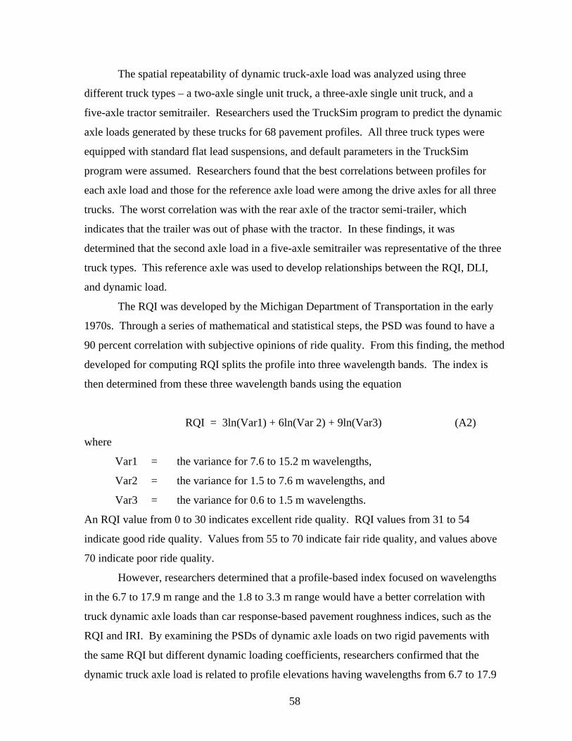
58

The spatial repeatability of dynamic truck-axle load was analyzed using three

different truck types – a two-axle single unit truck, a three-axle single unit truck, and a

five-axle tractor semitrailer. Researchers used the TruckSim program to predict the dynamic

axle loads generated by these trucks for 68 pavement profiles. All three truck types were

equipped with standard flat lead suspensions, and default parameters in the TruckSim

program were assumed. Researchers found that the best correlations between profiles for

each axle load and those for the reference axle load were among the drive axles for all three

trucks. The worst correlation was with the rear axle of the tractor semi-trailer, which

indicates that the trailer was out of phase with the tractor. In these findings, it was

determined that the second axle load in a five-axle semitrailer was representative of the three

truck types. This reference axle was used to develop relationships between the RQI, DLI,

and dynamic load.

The RQI was developed by the Michigan Department of Transportation in the early

1970s. Through a series of mathematical and statistical steps, the PSD was found to have a

90 percent correlation with subjective opinions of ride quality. From this finding, the method

developed for computing RQI splits the profile into three wavelength bands. The index is

then determined from these three wavelength bands using the equation

RQI = 3ln(Var1) + 6ln(Var 2) + 9ln(Var3) (A2)

where

Var1 = the variance for 7.6 to 15.2 m wavelengths,

Var2 = the variance for 1.5 to 7.6 m wavelengths, and

Var3 = the variance for 0.6 to 1.5 m wavelengths.

An RQI value from 0 to 30 indicates excellent ride quality. RQI values from 31 to 54

indicate good ride quality. Values from 55 to 70 indicate fair ride quality, and values above

70 indicate poor ride quality.

However, researchers determined that a profile-based index focused on wavelengths

in the 6.7 to 17.9 m range and the 1.8 to 3.3 m range would have a better correlation with

truck dynamic axle loads than car response-based pavement roughness indices, such as the

RQI and IRI. By examining the PSDs of dynamic axle loads on two rigid pavements with

the same RQI but different dynamic loading coefficients, researchers confirmed that the

dynamic truck axle load is related to profile elevations having wavelengths from 6.7 to 17.9

59

m, which excites the truck body bounce, and from 1.8 to 3.3 m, which excites the axle

bounce.

The new profile index was found according to linear random vibration theory, in

which the PSD of the truck response was obtained by multiplying the square of the truck

response function by the PSD of the surface profile. The variance of the truck response was

then found by considering only the frequency ranges of 1.5 to 4.0 and 8.0 to 15.0 Hz, which

correspond to the truck and axle bounces, respectively. The variance Vy is determined from

the following equation:

Vy = |G(w1)|2 V1 + |G(w2)|2 V2 (A3)

where

G(w1) = peak value of truck response function in the frequency range of 1.5 to 4.0 Hz,

G(w2) = peak value of truck response function in the frequency range of 8.0 to 15.0 Hz,

V1 = variance of the elevation in the frequency range of 1.5 to 4.0 Hz, and

V2 = variance of the elevation in the frequency range of 8.0 to 15.0 Hz.

Based on the standard deviation of the truck response and Eq. A3, the new roughness index,

DLI, is determined from the following equation:

DLI a V a V= +1 1 2 2 (A4)

where

V1 = variance of the profile elevation in the wavelength range of 6.7 to 17.9 m

corresponding to a frequency range of 1.5 to 4.0 Hz for a truck traveling at

96 kph,

V2 = variance of the profile in the wavelength range of 1.8 to 3.3 m

corresponding to a frequency range of 8.0 to 15.0 Hz for a truck traveling at

96 kph, and

a1, a2= weighting factors.

For convenience, researchers set a1 equal to one and a2 equal to 14, the value that gave the

highest correlation between DLI and dynamic loads. Therefore, the final equation for

computing DLI is:

DLI V V= +1 214 (A5)

According to the researchers, the use of DLI is beneficial in the following ways:

60

• DLI can differentiate between profiles that generate high dynamic loads and those

having the same RQI but generating low dynamic loads, and

• DLI can be used to decide the need for smoothing or correcting the profile of a given

section without running a truck simulation program.

Papagiannakis and Raveendran (1998) developed the roughness index for driving

expenditure (RIDE), which is compatible to the International Standards Organization (ISO)

standard on “exposure to whole-body vibration.” The two main requirements for the

development of the index were that it be related to the riding comfort of passenger cars and

heavy trucks and that it reflect the pavement roughness aspects that relate to the dynamic

axle loads generated by heavy trucks. Papagiannakis demonstrated in previous research that

the main contributor to the dynamic axle loads of heavy trucks is the vertical acceleration of

the sprung mass with no dependence on suspension type. This work was done with

instrumentation that measured both dynamic axle loads and sprung mass acceleration. Based

on this research, it became evident that a pavement roughness index based on sprung mass

acceleration would be preferable to one based on relative axle displacement, such as the IRI.

It was also determined from previous research that the calculation of an index based on

sprung mass acceleration is more efficient in the frequency domain than in the time domain,

and that a frequency domain transfer function with a resonant frequency of about 3 Hz and

corresponding amplitude of about 400 m/sec2/m is representative of the sprung mass

response exhibited by both heavy trucks and passenger cars.

The transfer function that was selected to be used as a reference in calculating RIDE

was determined from data obtained from an instrumented five-axle semitrailer truck on a

pavement of medium roughness at 80 kph. This selection was made in order to provide a

comparison to IRI, which is also calculated based on a speed of 80 kph. The power spectral

density of the sprung mass acceleration response was found by multiplying the PSD of the

pavement profile by the square of the reference frequency domain transfer function. The

new index, RIDE, was then found by integrating the PSD of the pavement profile over the

frequency range from 0 to 50 Hz. This gives the sum of the squares of the sprung mass

acceleration response of the reference vehicle. The square root of this integral divided by the

length of the pavement traveled results in a root-mean-square (RMS) of the acceleration

response per unit length, which is compatible with ISO 2631.

61

Hassan and McManus (2003) developed a new pavement roughness index that

represents the heavy-vehicle driver’s perception of pavement rideability using existing

profile data measured along the wheel paths of a passenger car. This was done by

conducting an assessment survey to gather truck drivers’ ratings of the ride quality of a

number of road sections with various roughness levels along a highway in rural Victoria,

Australia, on which there is a high percentage of heavy vehicle traffic. The data were then

analyzed by correlating the mean panel rating (MPR) to roughness content in different

wavebands of each road section. The roughness content that resulted in the highest

correlation was then used in developing the new index referred to as the profile index for

trucks (PIt).

Researchers performed PSD analyses on the road surface profile data using the

RoadRuf software developed by the University of Michigan Transportation Research

Institute (1997). Profile data were converted into slope values by subtracting adjacent

elevation readings and dividing by the sample interval. RMS values of profile slope in one-

third octave bands were then determined. The MPR was correlated with roughness contents

in different wavebands to identify wavelengths that influence ride perception. This analysis

showed that the waveband between 4.88 and 19.51 m gave the highest correlation with the

MPR. Thus, researchers used the roughness content in this band to establish the new index

given below:

PI PI PIt

OWP IWP=+( ) ( )2 2

2 (A6)

where

PIOWP = the average of the RMS values of the profile slope for the outer wheel

path, and

PIIWP = the average of the RMS values of the profile slope for the inner wheel

path.

An exponential transform was also used to develop a truck ride number (TRN) to

predict pavement ride quality, as perceived by heavy-vehicle occupants, from existing road

surface profile data. This index is given by the following equation:

TRN e PIt= −5 140 0 84( ) .

(A7)

Equation A7 gave the highest correlation coefficient between predicted TRN values and

actual MPR values. Another TRN equation was developed using IRI as the predictor of

62

MPR. This alternative equation was also found to be a good predictor of MPR, but not as

good as Eq. A7. The TRN equation based on IRI is given by:

TRN eIRIIRI= −5 118 70 0 9. ( ) .

(A8)

TRUCK TESTS ON INSTRUMENTED PAVEMENT SECTIONS Steven and de Pont (1998) conducted research at the Canterbury Accelerated

Pavement Testing Indoor Facility (CAPTIF) to investigate the relationship between the

dynamic loadings produced by different suspensions and the resultant pavement

performance. This research was done by comparing two different suspensions, whose

performance characteristics were at opposite ends of the spectrum, with the simulated

loading and vehicle emulator (SLAVE). The two SLAVE vehicles use standard

heavy-vehicle suspension components, which are equipped with half-axle assemblies that can

carry either single or dual tires. The SLAVE was fitted with suspensions similar to actual

heavy-vehicle components, with one vehicle having an air spring suspension with hydraulic

shock absorbers and the other having a multi-leaf steel spring.

After construction of a test pavement, 600 loading cycles of the SLAVE were applied

to condition it before any testing was done. Transverse profiles were taken at each station,

and longitudinal profiles were also measured with the Dipstick. The IRI values of the

profiles were calculated from the longitudinal profiles and were found to be 4.8 m/km and

4.1 m/km for the inner and outer wheel paths, respectively. Tire deflections and imprints

were measured at different applied load increments. Suspension stiffness was measured by

recording displacements as load increments were applied to characterize the natural

frequency and damping characteristics of the suspension.

The pavement started to show signs of deterioration at 60,000 loading cycles. The

rate of deterioration slowed down after 105 loading cycles. After completion of 2.5 × 105

cycles, all of the H-bar gages in the asphalt pavement had failed because strains measured in

the asphalt exceeded the capacity of the gages.

Researchers found that the pavement response was relatively constant during the

experiment. The IRI values varied only slightly throughout the test, and the dynamic load

coefficient (DLC) of the steel spring suspension is significantly higher than the air bag

suspension. It was concluded that the effect of the steel spring suspension was an increase in

the rate of pavement deterioration when compared to the air bag suspension.

63

Merrill, Blackman, and Ramdas (2002) conducted an international study to assess the

significance of vehicle dynamic loading on the performance and maintenance costs of road

pavements and bridges. This research arose from the results of a project, the Dynamic

Interaction between Vehicle and Infrastructure Experiment (DIVINE), sponsored by the

Organization for Economic Cooperation and Development, which was based on the limited

testing of a few pavements and bridges. Also considered in this research were the results of

the European Commission’s Cooperation in Science and Technology (EC COST)

Action 334, in which the effects of wide-single and dual tires on pavement wear were

examined.

EC COST Action 334 considered the effects of wide-base single and dual tire

assemblies on pavement damage, vehicle operating costs, vehicle safety and comfort, and the

environment, especially noise. Particular attention was paid to the effects of single tires,

wide-base single tires, and dual tires on pavement wear with respect to tire type and inflation

pressure. The study conducted by Merrill et al. included the measurement of pavement

response under dynamic loading, the measurement of contact stress distributions, and the

assessment of pavement wear through trafficking. It was conducted at TRL’s Pavement Test

Facility (PTF). Equipment at this facility can traffic pavements with loads up to 100 kN

(22.5 kip) at a maximum speed of 20 kph (12 mph) along a linear path.

Testing was conducted on a thin asphalt pavement, with a 100 mm layer of high

density macadam (HDM) road base, and on a medium pavement, with 100 mm of HDM road

base, 50 mm of dense bitumen macadam base course, and 50 mm of hot rolled asphalt

surfacing. Both sections were constructed on 225 mm of unbound granular sub-base. Six

tires were used in the study, which included four dual tires and two types of single tires. The

tires used were:

• 495/45R22.5 Michelin Energy XDA wide-base single,

• 385/65R22.5 Michelin X XZA wide-base single,

• 295/60R22.5 Michelin X XDA dual pair,

• 295/80R22.5 Michelin X Pilote XDA dual pair,

• 315/70R22.5 Michelin X XDA dual pair, and

• 315/80R22.5 Michelin X Pilote XDA dual pair.

To measure the effects that different tire types, inflation pressures, and wheel loads

have on the pavement structures, the subgrade was instrumented with soil strain gages placed

64

150 mm below the surface of the subgrade prior to laying the sub-base. These gages were

oriented to measure the transient vertical compressive component of strain for all six tire

types for a variety of loads and inflation pressures. The wheel of the heavy vehicle was also

moved laterally to measure the strain in relation to the position of the load. Measurements

were also taken at varying tire pressures, which ranged between 5 and 10 bars for each tire.

The Tekscan Industrial Sensing (I-Scan) system was used to measure the load distribution for

the different tire types at different loads and inflation pressures with a low resolution mat.

It was found that subgrade strains under the single tires diminish more rapidly as the

tire moved away from the central position when compared to the dual tire assemblies. The

difference was attributed to the differing contact areas in regard to the different tire types, but

the difference diminished with an increase in pavement thickness. Inflation pressure had a

negligible effect on subgrade strain, even with differentially inflated dual tires. Subgrade

strain was measured with a change in load, and it varied linearly with both pavement

thicknesses. However, the magnitude of the strain was higher for single tires than for dual

tires. Also, the gradient of change was higher for the single tires than for the dual tires.

In general, the pressure increased in the center of the contact areas for all tires with a

negligible change at the edges of the tires. It was determined that the 385/65R22.5 Michelin

X XZA wide-base single tire had a concentration of pressure in the center of the distribution,

but the highest pressures are scattered. This difference was probably due to tread effects.

The 495/45R22.5 Michelin Energy XDA wide-base single tire had three areas of high

pressure, with a constant area of high pressure in the center and two areas closer to the edge

of the tire. Also evaluated in this experiment was pavement wear under accelerated

trafficking using the heavy-vehicle simulator at TRL and the two single tires. The following

criteria were considered in this evaluation: rutting, deformation, subgrade stain, and

cracking. The tires used for testing were loaded to 44 kN and to the manufacturers’

recommended inflation pressures. Over 110,000 passes were applied to each pavement with

the thinner pavement failing at 57,000 passes.

Deformation was measured at intervals during breaks in the trafficking using an

optical level and measuring staff, which behaved as expected. Inferences were made from

the deformation profiles in that there were fewer formations of small shoulders in the thin

pavements on either side of the rut than for the thicker pavements. This observation

indicated a punching action as opposed to a layer deformation. The ratio for the 385 to the

65

495 single tires on each pavement thickness showed that there was a much smaller difference

between the two tire types on the thin pavement than on the thicker pavements. This was

attributed to the failure of the thin pavement.

Rut depths were measured using straightedge and wedge, which differ from the

optical levels because the reference point is not fixed and is a line that joins the two highest

points over a 2-meter distance. Again, the rate of rutting was compared for the 385 and 495

single tires. The depth ratio reached 1.8 for the 100 mm pavement and reduced to 1.2 at the

point of failure. The ratio for the 200 mm pavement reached 2.5 before reducing to 1.7

beyond 110,000 passes. The 200 mm pavement experienced about 40 percent less rutting

with the 495 single tire than with the 385 single tire. Since no dual tires were tested in this

part of the study, an attempt was made to estimate the likely outcomes for the accelerated

testing with all tires.

Subgrade strain measurements were taken at the end of the trafficking and were

compared to the measurements made at 2000 passes. The 100 mm pavement failed rapidly,

and the strain increased by 5 times after 57,000 passes. The subgrade strain only doubled for

the 200 mm pavement at 300,000 passes; however, there was significant difference between

the two types of single tires.

Pavements were also monitored for signs of distress, such as cracking. The thin

pavement for both tire types showed signs of distress after 15,000 passes, and the full length

and width of the thin pavement were distressed after 30,000 passes. No visual signs of

distress were observed for the 200 mm pavement.

Another part of this project accepted the detailed information available in regard to

dynamic loading behavior with respect to the behavior of the vehicle. This study sought to

link the contribution of dynamic loading by commercial vehicles to pavement wear in order

to quantify the relationship between profile unevenness and the deterioration caused by

dynamic loading effects, and in order to assess any significant repeat loadings on the

development of localized deterioration. This objective was accomplished by examining the

loading effects of actual commercial traffic on 10 in-service flexible and flexible composite

pavements with a range of profile unevenness, commercial traffic, and structural strengths.

Pavement deterioration was assessed from changes in longitudinal profile and rutting, and the

dynamic loading was measured using an instrumented heavy goods vehicle.

66

The 10 sites were surveyed using a variety of equipment. These included an

instrumented five-axle articulated lorry, TRL’s high-speed survey vehicle (HSV), and the

falling weight deflectometer (FWD). The instrumented lorry was used to measure the spatial

repeatability and amplitudes of dynamic loading. The HSV uses laser sensors and a specially

programmed computer to measure profile amplitude and wheel track rut depth, and the FWD

was used to collect pavement deflection data. The results of this survey indicated a small but

significant link between dynamic loading and change in road roughness.

The results of this research study show significant differences between tire types, but

the thin pavements tested had some bearing on these results. The subgrade strain is

significantly reduced with pavement thickness, so it was concluded that the effect of tire type

on subgrade strain is negligible. The results of the accelerated trafficking tests showed that

the 385/65R22.5 Michelin X XZA wide-base single tire consistently produced more wear

than the 495/45R22.5 Michelin Energy XDA wide-base single tire under the same

conditions. The rutting behavior was the most significantly affected by differences in tire

types. Based on these results, it was determined that the single tires would have produced

1.5 to 2.5 times the deformation potential of the dual tires.

TRUCK SURVEYS

Wang and Machemehl (2003) conducted a survey to characterize in-service truck

configurations on Texas highways. More specifically, they sought to characterize the

in-service truck tire pressures on trucks and to identify factors that might be related to

differences in tire pressure. To conduct this study, a three-factor factorial experiment was

designed in which the state was broken up into six geographic regions. These regions were:

Lubbock-Midland, Dallas, Houston, San Antonio-Austin, Corpus Christi, and the border

areas. Also considered were two highway classes and two highway directions. A total of

623 trucks, classified according to the FHWA Truck Size and Weight Codes, were selected

for the truck configuration survey and were tested for tire inflation pressure, tire temperature,

tire size, and tire manufacturer.

Laboratory experiments and linear regressions were conducted on the data collected

to establish the relationship between tire inflation pressure and tire temperature. The

relationship determined by researchers is given by the following equation:

67

P P T T2 1 2 10 22= + −. ( ) (A9)

where P1 and P2 are tire inflation pressures in psi corresponding, respectively, to tire

temperatures T1 and T2 in °F.

This study sought to characterize truck tire pressures across Texas and to verify if tire

pressures were related to factors like geographic area, highway class, and highway direction.

However, since tire temperature is directly affected by air and pavement temperatures, it was

necessary to correct the tire pressure data to a standard temperature of 60 °C (140 °F) in

order to characterize the relationship between tire pressure and tire temperature. In order to

do this, researchers used the following equations:

P P T2 1= + α ∆ (A10)

α = =PT

n RV

1

1

(A11)

where

R = ideal gas constant,

P1 = gas pressure in atmospheres,

T1 = absolute gas temperature in °K,

V = gas volume in liters,

N = number of gas molecules in moles, and

α = coefficient of the relationship between pressure and temperature.

To obtain values for α, inflated truck tires were tested at different temperatures in the

laboratory, and a linear regression was run using the temperature and pressure data. The

average α was found to be 2.73 kPa/°C.

A t-test was conducted to check whether there is a significant difference in tire

inflation pressures between loaded and empty trucks. Table A1 shows the results of this test.

The results indicate a significant difference in tire inflation pressures between loaded and

empty trucks.

A t-test was also conducted on the effect of highway direction versus truck tire

pressure. No significant differences were found. The effect of geographic region was found

to match with the 1986 survey conducted by Roberts et al. Geographic regions were ranked

in ascending order as follows: Border, San Antonio-Austin, Houston, Dallas, Corpus Christi,

and Lubbock-Midland.

68

Table A1. Summary of t-test on Difference in Truck Tire Inflation Pressures between Loaded and Empty Trucks (Wang and Machemehl, 2000).

Test Group Sample Size

Mean (kPa)

Standard Dev. (kPa) Test Statistics

435 loaded trucks 435 trucks 756.9 60.2 169 empty trucks 169 trucks 718.2 69.1 t=6.90 Z95%=1.96

A one-way analysis of variance (ANOVA) was conducted for the comparison of

border and non-border areas with respect to truck tire inflation pressure. The results of this

test (Table A2) show a significant difference in tire inflation pressures between border and

non-border areas, as indicated from the very small p-value given in the table. The low tire

pressures in the border areas could be attributed to the North American Free Trade

Agreement, which prohibits Mexican trucks from operating in the United States. More than

50 percent of the trucks selected in the border areas were empty.

A two-way ANOVA test was conducted to evaluate the effect of geographic area and

highway class on truck tire inflation pressures. The results (Table A3) show the effects of

geographic area and highway class to be significant, indicating that trucks in different

geographical areas had different tire inflation pressures, and similarly for trucks in different

highway classes.

A comparison was also made among the five axles of 500 3-S2 trucks selected using

a one-way ANOVA. All tires of the same axle were pooled and averaged to represent the

axle tire inflation pressure. The test results given in Table A4 show a significant difference

among the five axles of the 3-S2s. The most significant of these results is that the first axle,

which is the steering, possessed a much higher axle tire inflation pressure than the other four.

Also, axles 2 and 3, which are the drive axles, possessed almost the same mean and variance

values. Axles 4 and 5, which are the trailer axles, were different, but many of the trailers

surveyed had a different license plate number than the tractor and were poorly maintained.

The study concluded that factors such as axle weight, tire temperature, geographic

area, highway class, and axle type are related to tire inflation pressure. The results also

suggest that trucks operating with high axle weights over long-haul distances traveling

interstate highways with high operating temperatures will have higher tire inflation pressures

in particular geographic areas. Lastly, it was determined that the steering axles have the

highest tire inflation pressures of all the truck axles.

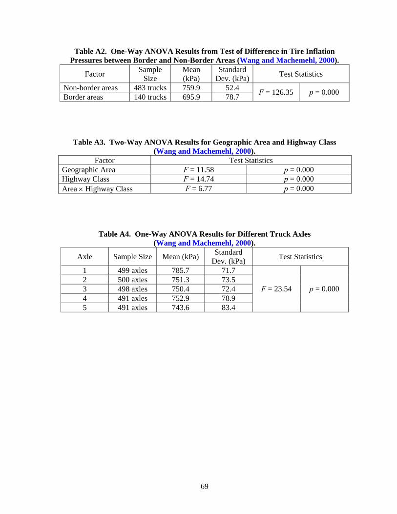
69

Table A2. One-Way ANOVA Results from Test of Difference in Tire Inflation Pressures between Border and Non-Border Areas (Wang and Machemehl, 2000).

Table A3. Two-Way ANOVA Results for Geographic Area and Highway Class (Wang and Machemehl, 2000).

Factor Test Statistics Geographic Area F = 11.58 p = 0.000 Highway Class F = 14.74 p = 0.000 Area × Highway Class F = 6.77 p = 0.000

Table A4. One-Way ANOVA Results for Different Truck Axles (Wang and Machemehl, 2000).

Axle Sample Size Mean (kPa) Standard Dev. (kPa) Test Statistics

1 499 axles 785.7 71.7 2 500 axles 751.3 73.5 3 498 axles 750.4 72.4 4 491 axles 752.9 78.9 5 491 axles 743.6 83.4

F = 23.54 p = 0.000

Factor Sample Size

Mean (kPa)

Standard Dev. (kPa) Test Statistics

Non-border areas 483 trucks 759.9 52.4 Border areas 140 trucks 695.9 78.7 F = 126.35 p = 0.000

Technical Report Documentation Page 1. Report No. 2 ... · TRUCK INSTRUMENTATION FOR DYNAMIC LOAD...

Documents

Transcript of Technical Report Documentation Page 1. Report No. 2 ... · TRUCK INSTRUMENTATION FOR DYNAMIC LOAD...