Technical Report CSTN-065 Exploiting Graphical Processing ...

Technical Report CSTN-065

Exploiting Graphical Processing Units for Data-Parallel ScientificApplications

A. Leist, D. P. Playne and K. A. Hawick†

Computer Science, Institute of Information and Mathematical Sciences,Massey University, Albany, Auckland, New Zealand

December 2008

Abstract

Graphical Processing Units (GPUs) have recently attracted attention for scientific applications such as particle simula-tions. This is partially driven by low commodity pricing of GPUs but also by recent toolkit and library developments thatmake them more accessible to scientific programmers. We report on two further application paradigms – regular mesh fieldequations with unusual boundary conditions and graph analysis algorithms – that can also make use of GPU architectures.We discuss the relevance of these application paradigms to simulations engines and games. GPUs were aimed primarilyat the accelerated graphics market but since this is often closely coupled to advanced game products it is interesting tospeculate about the future of fully integrated accelerator hardware for both visualisation and simulation combined. Aswell as reporting speed-up performance on selected simulation paradigms, we discuss suitable data-parallel algorithms andpresent code examples for exploiting GPU features like large numbers of threads and localised texture memory. We find asurprising variation in the performance that can be achieved on GPUs for our applications and discuss how these findingsrelate to past known effects in parallel computing such as memory speed-related super-linear speed-up.

Keywords: data-parallelism; GPUs; field equations; graph algorithms; CUDA.

1 INTRODUCTION

Arguably, Data-Parallel computing went through its last important “golden age” in the late 1980s and early 1990s [1]. Thatera saw a great many scientific applications ported to the then important massively parallel and data-parallel supercomputerarchitectures such as the AMT DAP [2] and the Thinking Machines Connection Machine [3,4]. The era also saw successfulattempts at portable embodiments of data-parallel computing ideas into software libraries, kernels [5, 6] and programminglanguages [7, 8, 9, 10]. Much of this software still exists and is used, but was perhaps somewhat overshadowed by thesubsequent era of coarser-grained multi-processor computer systems – perhaps best embodied by cluster computers, andalso by software to exploit them such as message-passing systems like MPI [11]. We have since seen some blending togetherof these ideas in software languages and systems like OpenMP [12]. We are currently in an era where wide-ranging parallelcomputing ideas are being exploited successfully in multi-core central processing units (CPUs) and of course in GPUs – asdiscussed in this article.

Graphical Processing Units (GPUs) [13] have emerged in recent year as an attractive platform for optimising the speed of anumber of application paradigms relevant to the games and computer-generated character animation industries [14]. Whilechip manufacturers have been successful in incorporating ideas in parallel programming into their family of CPUs, in-evitably due to the need for backwards compatibility, it has not been trivial to make major advances with complex backwardcompatible CPU chips. The concept of the GPU as a separate chip with fewer legacy constraints is perhaps one explanationfor the recent dramatic improvements in the use of parallel hardware and ideas at a chip level.

1

In principle, GPUs can of course be used for many parallel applications in addition to their original intended purpose ofgraphics processing algorithms. In practice however, it has taken some relatively recent innovations in high-level program-ming language support and accessibility for the wider applications programming community to consider using GPUs in thisway [15, 16, 17]. The term general-purpose GPU programming (GPGPU) [14] has been adopted to describe this rapidlygrowing applications level use of GPU hardware. Exploiting parallel computing effectively at an applications level remainsa challenge for programmer. In this article we focus on two broad application areas - partial differential field equationsand graph combinatorics algorithms and explore the detailed coding techniques and performance optimisation techniquesoffered by the Compute Unified Device Architecture (CUDA) [17] GPU programming language. NVIDIA’s CUDA hasemerged in recent months as one of the leading programmer tools for exploiting GPUS. It is not the only one [18,19,20,21],and inevitably it builds on many past important ideas, concepts and discoveries in parallel computing.

In the course of our group’s research on complex systems and simulations we have identified a number of scientific applica-tion paradigms such as those based on particles, field models, and on graph network representations [22]. The use of GPUsfor paradigm of N-Body particle simulation has already been well reported in the literature already [23, 24], and hence inour present article we focus on complex field-based and graph-based scientific application examples.

In section 2 we present some technical characteristics of GPUs, general ideas and explanatory material on how some GPUswork and how they can be programmed with a language like CUDA. We present some of our own code fragments by wayof explanation for exploiting some of the key features of moderns GPUs such as the different sorts of memory and the useof and groupings of multiple parallel executing threads.

In section 3 we present some ideas, code examples and performance measurements for a specific partial differential equa-tion simulation model - the Cahn-Hilliard field equation as used for simulating phase separation in material systems. Weexpected this would parallelise well, and although we can obtain good results in the right system size regime, there areinteresting and surprising variations that arise from the nature of a practical simulation rather than a carefully chosen toy orbenchmark scenario.

A problem area that we expected to be much more difficult to achieve good performance in, is that of graph combinatoricproblems. In section 4 we focus on the all-pairs shortest path problem in graph theory as highly specific algorithm used insearching, navigation and other problems relevant to the games and computer generated character generation industries.

In both these problem areas we have been able to use the power of GPU programming to obtain some scientifically usefulresults in complex systems, scaling and growth research. In this present article we focus on how the parallel coding wasdone and how the general ideas might be of wider use to the scientific simulations programming community.

We offer some ideas and speculations as to future directions for GPUs and their exploitation at a software level for scientificapplications in section 6.

2 GPU FEATURES

GPU architectures contain many processors which can execute instructions in parallel. These parallel processors provide theGPU with the high-performance parallel computational power. To make use of this parallel computational power, a programexecuting on the GPU must be decomposed into many parallel threads. Parallel decomposition of computational problemsis a widely researched topic and is not discussed in detail here. However, one specific condition of parallel decompositionfor GPUs is the number of threads the problem should be split into. As GPUs is capable of executing a large number ofthreads simultaneously, it is generally advantageous to have as many threads as possible. A large number of threads allowsthe GPU to maximise the efficiency of execution.

2.1 NVIDIA Multiprocessor Architecture

To maximise performance, it is important to maximise the utilisation of the available computing resources as described inthe CUDA Programming Guide (PG) [25]. This means that there should be at least as many thread blocks as there are

2

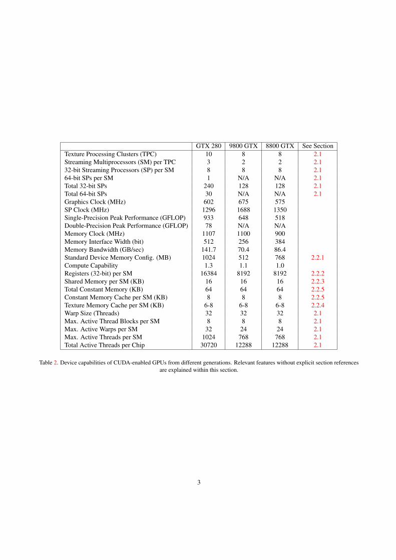
GTX 280 9800 GTX 8800 GTX See SectionTexture Processing Clusters (TPC) 10 8 8 2.1Streaming Multiprocessors (SM) per TPC 3 2 2 2.132-bit Streaming Processors (SP) per SM 8 8 8 2.164-bit SPs per SM 1 N/A N/A 2.1Total 32-bit SPs 240 128 128 2.1Total 64-bit SPs 30 N/A N/A 2.1Graphics Clock (MHz) 602 675 575SP Clock (MHz) 1296 1688 1350Single-Precision Peak Performance (GFLOP) 933 648 518Double-Precision Peak Performance (GFLOP) 78 N/A N/AMemory Clock (MHz) 1107 1100 900Memory Interface Width (bit) 512 256 384Memory Bandwidth (GB/sec) 141.7 70.4 86.4Standard Device Memory Config. (MB) 1024 512 768 2.2.1Compute Capability 1.3 1.1 1.0Registers (32-bit) per SM 16384 8192 8192 2.2.2Shared Memory per SM (KB) 16 16 16 2.2.3Total Constant Memory (KB) 64 64 64 2.2.5Constant Memory Cache per SM (KB) 8 8 8 2.2.5Texture Memory Cache per SM (KB) 6-8 6-8 6-8 2.2.4Warp Size (Threads) 32 32 32 2.1Max. Active Thread Blocks per SM 8 8 8 2.1Max. Active Warps per SM 32 24 24 2.1Max. Active Threads per SM 1024 768 768 2.1Total Active Threads per Chip 30720 12288 12288 2.1

Table 2. Device capabilities of CUDA-enabled GPUs from different generations. Relevant features without explicit section referencesare explained within this section.

3

streaming multiprocessors (SM) in the device. And since each SM consists of 8 scalar processor cores—also called Stream-ing Processors (SP)—a GeForce GTX 280 can execute a total of 240 threads simultaneously. However, the multiprocessorSIMT unit groups the threads in a block into so called warps, each consisting of 32 parallel threads that are created, man-aged, scheduled, and executed together. A warp is the smallest unit of execution in CUDA. Thus, at least 960 threads shouldbe created to keep a GTX 280 busy. (See PG chpts. 3.1 and 5.2)

Furthermore, to enable the thread scheduler to hide latencies incurred by thread synchronisations (4 clock cycles), issuingmemory instruction for a warp (4 clock cycles), and especially by accessing the device memory (400-600 clock cycles), aneven larger number of active threads is needed per multiprocessor. As listed in table 2, the latest generation of GeForceGPUs supports up to 30,720 active threads (30 SMs × 32 warps × 32 threads per warp), significantly improving thethread scheduler’s capability to hide latencies compared to the 12,288 active threads supported by the previous generations.Memory-bound kernels in particular require a large number of threads to maximise the utilisation of the computing resourcesprovided by the GPU. (See PG chpts. 5.1.1 and 5.2)

There are several possible ways to organise the threads once the thread count exceeds one warp per block per SM. Eitherthe number of blocks per multiprocessor, the block size, or both can be increased, up to the respective limits. Increasing thenumber of active blocks on a multiprocessor to at least twice the number of multiprocessors allows the thread scheduler tohide thread synchronisation latencies and also device memory reads/writes if there are not enough threads per block to coverthese. The shared memory and registers of a SM are shared between all active blocks that reside on this multiprocessor.Thus, for two thread blocks to simultaneously reside on one multiprocessor, each of the blocks can use at most 1

2 of theavailable resources. (See PG chpt. 5.2)

But having even more than the maximum number of total active thread blocks on the device can be a good idea, as it willallow the kernel to scale to future hardware with more SMs or more local resources available to each SM. If scaling to futuredevice generations is desired, then it is advisable to create hundreds or even thousands of thread blocks. (See PG chpt. 5.2)

Larger block sizes, on the other hand, have advantages when threads have to communicate and when the execution hasto be synchronised at certain points. Threads within the same block can communicate through shared memory and callthe syncthreads() barrier function, which guarantees that none of the threads proceeds before all other threads have alsoreached the barrier. The block size should always be a multiple of the warp size to avoid partially filled warps and becausethe number of registers used per block is always rounded up to the nearest multiple of 32. Choosing multiples of 64 is evenbetter, as this helps the compiler and thread scheduler to achieve best results avoiding register memory bank conflicts. (SeePG chpts. 2.1, 3.1, 5.1.2.5, 5.1.2.6, and 5.2)

The maximum block size is 512 threads for all CUDA-enabled GPUs released so far. Thus, to reach the maximum numberof active threads supported on a GTX 280, both the number of blocks and the block size have to be increased. Themultiprocessor occupancy is a metric that states this ratio of active threads to the maximum number of active threadssupported by the hardware. The definition is given in equation 1. (See PG chpts. 2.1 and 5.2)

Occupancy =number of active warps per multiprocessor

maximum number of active warps per multiprocessor(1)

While trying to maximise the multiprocessor occupancy is generally a good idea, a higher occupancy does not always meanbetter performance. The higher the value, the better the scheduler can hide latencies, thus making this metric especiallyimportant for memory-bound kernels. However, other factors that can have a large impact on the performance are notreflected, like the ability of more threads to communicate via shared memory when the block size is larger. Thus, ifpossible, performance should always be measured for various block sizes to determine the best value for a specific kernel.

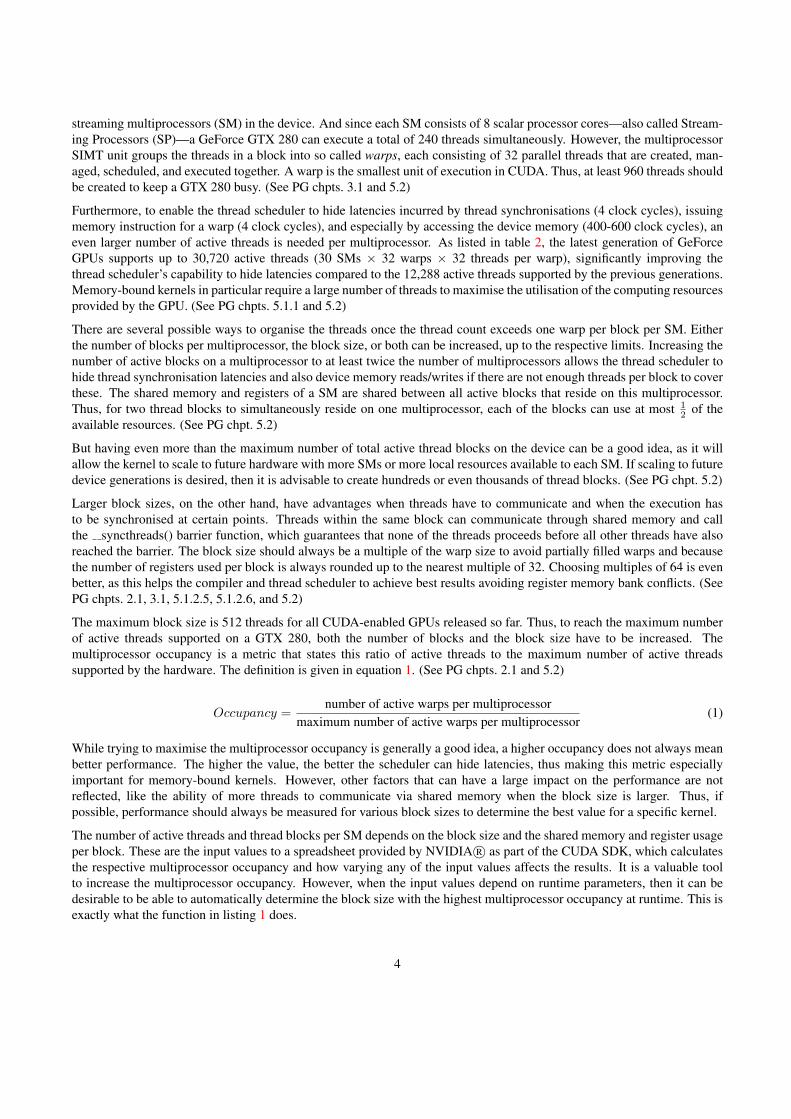
The number of active threads and thread blocks per SM depends on the block size and the shared memory and register usageper block. These are the input values to a spreadsheet provided by NVIDIA R© as part of the CUDA SDK, which calculatesthe respective multiprocessor occupancy and how varying any of the input values affects the results. It is a valuable toolto increase the multiprocessor occupancy. However, when the input values depend on runtime parameters, then it can bedesirable to be able to automatically determine the block size with the highest multiprocessor occupancy at runtime. This isexactly what the function in listing 1 does.

4

Listing 1: Implementation of the occupancy calculation to determine the maximum multiprocessor occupancy on the avail-able graphics hardware for a given register and shared memory usage.

/∗ ∗∗ R e t u r n s t h e number o f t h r e a d s per b l o c k t h a t g i v e s t h e h i g h e s t∗ m u l t i p r o c e s s o r occupancy . P r e f e r s l a r g e r t h r e a d b l o c k s over s m a l l e r∗ ones w i t h t h e same occupancy . NOTE: Always r e t u r n s 32 i f c o m p i l e d∗ f o r d e v i c e e m u l a t i o n ( t h e −dev iceemu f l a g i s pas se d t o t h e∗ c o m p i l e r ) .∗∗ Params : d e v i c e P r o p The d e v i c e p r o p e r t i e s .∗ r e g i s t e r s The number o f r e g i s t e r s needed by each t h r e a d .∗ sharedMemPerThread The sh are d memory needed per t h r e a d ( b y t e s ) .∗ sharedMemPerBlock The sh ar ed memory needed per b lock , i n d e p e n d e n t∗ o f t h e number o f t h r e a d s ( b y t e s ) .∗ /

i n t maxOccupancy ( cudaDev iceProp ∗ dev i ce P rop , i n t r e g i s t e r s ,i n t sharedMemPerThread , i n t sharedMemPerBlock ) {

/ / t h e v a l u e s f o r compute c a p a b i l i t y 1 . 0i n t l i m i t B l o c k s P e r M P = 8 ;i n t l imi tWarpsPerMP = 2 4 ;/ / a d j u s t t h e s e base v a l u e s a c c o r d i n g t o t h e a c t u a l compute c a p a b i l i t yi f ( dev i ceP rop−>major >= 1 && dev iceP rop−>minor >= 2) { / / 1 . 2

l imi tWarpsPerMP = 3 2 ;}

i n t l i m i t T h r e a d s P e r W a r p = d ev i ceP rop−>warpSize ;s i z e t l imitSharedMemPerMP = dev i ceP rop−>sharedMemPerBlock ;i n t l i m i t R e g i s t e r s P e r M P = dev i ceP rop−>r e g s P e r B l o c k ;

double maxOccupancy = 0 . 0 ;i n t nThreadsMaxOccupancy = 0 ;f o r ( i n t nThreads = 512 ; nThreads >= 3 2 ; nThreads −= 32) {

/ / t h e sh ar ed memory needed f o r t h i s b l o c k s i z ei n t sharedMem = sharedMemPerBlock + sharedMemPerThread ∗ nThreads ;

i n t myWarpsPerBlock = c e i l ( ( double ) nThreads / ( double ) l i m i t T h r e a d s P e r W a r p ) ;i n t mySharedMemPerBlock = n e x t M u l t i p l e O f P o w e r 2 ( sharedMem , 5 1 2 ) ;i n t myRegsPerBlock = n e x t M u l t i p l e O f P o w e r 2 ( myWarpsPerBlock ∗ 2 , 4 )∗ 16 ∗ r e g i s t e r s ;

i n t l imitedByMaxWarpsPerMP = min ( l imi tB locksPerMP ,( i n t ) f l o o r ( ( double ) l imi tWarpsPerMP

/ ( double ) myWarpsPerBlock ) ) ;

i n t l imitedBySharedMemPerMP ;i f ( sharedMem > 0) {

l imitedBySharedMemPerMP = f l o o r ( ( double ) l imitSharedMemPerMP/ ( double ) mySharedMemPerBlock ) ;

} e l s e {l imitedBySharedMemPerMP = l i m i t B l o c k s P e r M P ;

}

i n t l i m i t e d B y R e g i s t e r s P e r M P ;i f ( r e g i s t e r s > 0) {

l i m i t e d B y R e g i s t e r s P e r M P = f l o o r ( ( double ) l i m i t R e g i s t e r s P e r M P

5

/ ( double ) myRegsPerBlock ) ;} e l s e {

l i m i t e d B y R e g i s t e r s P e r M P = l i m i t B l o c k s P e r M P ;}

i n t a c t i v e T h r e a d B l o c k s P e r M P = min ( limitedByMaxWarpsPerMP ,min ( limitedBySharedMemPerMP ,

l i m i t e d B y R e g i s t e r s P e r M P ) ) ;i n t act iveWarpsPerMP = a c t i v e T h r e a d B l o c k s P e r M P ∗ myWarpsPerBlock ;double occupancy = ( double ) ac t iveWarpsPerMP / ( double ) l imi tWarpsPerMP ;

i f ( occupancy > maxOccupancy ) {maxOccupancy = occupancy ;nThreadsMaxOccupancy = nThreads ;

}}

# i f d e f DEVICE EMULATIONnThreadsMaxOccupancy = 3 2 ;

# e n d i f

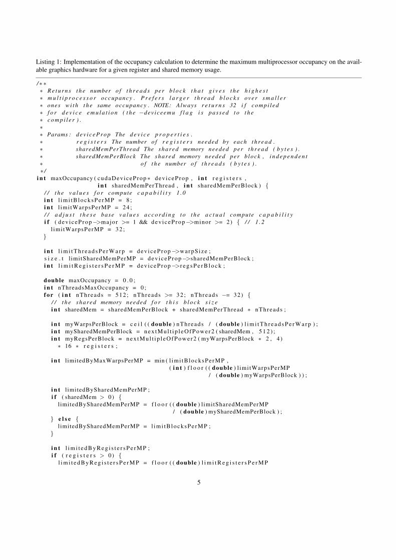
re turn nThreadsMaxOccupancy ;}

2.2 Memory

GPUs contain several types of memory that are designed and optimised for different purposes. Although the optimisationfeatures for the memory types is focused towards the specific tasks of the graphics pipeline, their features can be utilised forother purposes. Using the type of memory best suited to the task can provide significant performance benefits. The memoryaccess patterns used to retrieve/store data from these memory locations is equally important as the type of memory used.Correct access patterns are critical to the performance of the GPU program. CUDA-enabled GPUs provide access to sixdifferent types of memory that are stored both on-chip (within a multiprocessor) and on the device.

Global Memory is part of the device memory. It is the largest memory on the GPU and is accessible by every thread in theprogram. However, it has no caching and has the slowest access time of any memory type - approximately 200-400clock cycles. Lifetime = application. (See PG chpt. 5.1.2.1)

Registers are stored on-chip and are the fastest type of memory. The registers are used to store the local variables of asingle thread and can only be accessed by that thread. Lifetime = thread. (See PG chpt. 5.1.2.6)

Local Memory does not represent an actual physical area of memory, instead it is a section of device memory used whenthe variables of a thread do not fit within the registers available. Lifetime = thread. (See PG chpts. 4.2.2.4 and 5.1.2.2)

Shared Memory is fast on-chip memory that is shared between all of the threads within a single block. It can be used toallow the threads within a block to co-operate and share information. Lifetime = block. (See PG chpts. 4.2.2.3 and5.1.2.5)

Texture Memory space is a cached memory region of global memory. Every SM has its own texture memory cache on-chip. Device memory reads are only necessary on cache misses, otherwise a texture fetch only costs a read from thetexture cache. Lifetime = application. (See PG chpts. 5.1.2.4 and 5.4)

Constant Memory space is a cached, read-only region of device memory. Like the texture cache, every SM has its ownconstant memory cache on-chip. Device memory reads are only necessary on cache misses, otherwise a constantmemory read only costs a read from the constant cache. Lifetime = application. (See PG chpt. 5.1.2.3)

6

The access times to these types of memory depend on the access pattern used. The access patterns and optimal uses for thetypes of memory are now discussed.

2.2.1 Global Memory Access

Global memory has the slowest memory access times of any type of memory (200 - 400 clock cycles). Although the actualtime taken to access global memory cannot be reduced, it is possible to increase overall performance by combining theglobal memory transactions of the threads within the same half-warp into one single memory transaction. This process isknown as coalescing and can greatly increase the performance of a GPU program.

Global memory transactions can be coalesced if sequential threads in a half-warp access 32-, 64- or 128-bit words fromsequential addresses in memory. These sequential address depend on the size of the words accessed, ie each address mustbe the previous address plus the size of the word. 32- and 64-bit transcations are coalesced into a single transaction of64-/128-bytes and 128-bit transactions are coalesced into two 128-byte transactions. Coalesced memory access provides alarge performance improvement over the 16 global memory transactions required for non-coalesced memory access. (SeePG chpt. 5.1.2.1 for the detailed requirements and the differences between compute capabilities.)

Sometimes it is not possible to access global memory in a coalesced fashion. For instance, let us assume we have an arrayof sub-arrays of varying lengths. Storing this structure as a two-dimensional CUDA array would waste a lot of space if thearray lengths vary considerably. Thus, we store it as a one-dimensional array with the index of the first element of eachsub-array being pointed to by a second array. Furthermore, the first sub-array element specifies the length of the respectivearray. If each thread iterates over one of these sub-arrays, then the access is uncoalesced, resulting in many inefficientmemory transactions.

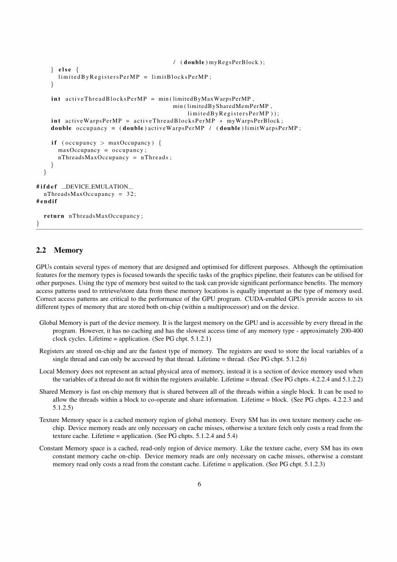
One way to improve the use of the memory bandwidth is to use a built in vector type like int4 as the type of the array. This issimply a correctly aligned struct of 4 integer values. We always group 4 elements of a sub-array into one such struct. Everysub-array begins with a new struct, thus some space is wasted if the length of a sub-array plus one for the length element isnot a multiple of 4. The advantages are that now four values (i.e. 16 bytes) can be read in one memory transaction insteadof only one and only a single instruction is required to write these values to registers. Listing 2 illustrates how a thread caniterate over a sub-array starting at index structArrayIdx.

Listing 2: Using the built in vector types to take advantage of the full memory bandwidth.

i n t 4 m y S t r uc t = s t r u c t A r r a y [ s t r u c t A r r a y I d x ] ;i n t n I t e r a t i o n s = m y S t r u c t . x ;f o r ( i n t i d x = 1 ; i d x <= n I t e r a t i o n s ; i d x ++) {

i n t s t r u c t I d x = i d x % 4 ;i n t v a l u e ;i f ( s t r u c t I d x == 0) {

m y S t ru c t = s t r u c t A r r a y [++ s t r u c t A r r a y I d x ] ; / / l oad t h e n e x t v e c t o rv a l u e = m y S t ru c t . x ;

} e l s e i f ( s t r u c t I d x == 1) {v a l u e = m y S t ru c t . y ;

} e l s e i f ( s t r u c t I d x == 2) {v a l u e = m y S t ru c t . z ;

} e l s e i f ( s t r u c t I d x == 3) {v a l u e = m y S t ru c t .w;

}. . .

}

One thing that should be considered when iterating over arrays of varying length is warp divergence. That is, threads withina warp taking diverging branches, or in this case iterating over a different number of elements. Warp divergence can reduceperformance significantly, as the SIMT-model forces diverging branches within a warp to be serialised. In this example,

7

branch divergence can be reduced if the sub-arrays are organised so that the threads of the same warp process arrays ofapproximately the same length.

2.2.2 Registers and Local Memory

Registers and local memory are used to store the variables used by the threads of the program. The very fast registers areused first, however if the variables of the threads cannot fit into the registers then local memory must be used. Fetchingvalues from local memory requires access to the global memory which is always coalesced but is much slower than accessingthe registers. Therefore it is desirable to structure the code such that all the local variables can fit within the registers. It isoften more efficient to perform the same calculation several times within a thread to avoid storing values in local memory.

As long as no register read-after-write dependencies or register memory bank conflicts occur, accessing a register costs zeroextra clock cycles per instruction. Delays due to read-after-write dependencies can be ignored if at least 192 active threadsper multiprocessor exist to hide them. Registers are used to store the local variables of a thread and can not be used to sharedata between threads.

2.2.3 Shared Memory

Shared memory can be used to reduce the amount of global memory access required. If two or more threads within thesame block must access the same piece of data, shared memory can be used to transfer data between them. The remainingthreads can then access this value from the faster shared memory instead of through global memory accesses.

Shared memory is divided into 16 banks (compute capability 1.x), which are equally sized memory modules that can beaccessed simultaneously. Successive 32-bit words are assigned to successive banks and each bank has a bandwidth of 32 bitsper two clock cycles. A half-warp consisting of 16 threads and executing in two clock cycles only needs one shared memoryrequest to read or write data as long as no bank conflicts occur. Thus, it is important to schedule shared memory requests soas to minimise bank conflicts. Writes to shared memory are guaranteed to be visible by other threads after a syncthreads()call.

Shared memory can either be allocated statically or dynamically. The total size of dynamically allocated shared memory isdetermined at launch time as an optional parameter to the execution configuration of the kernel. If more than one variablepoints to addresses within the memory range allocated in this fashion, then this has to be done by using appropriate offsetsas illustrated in listing 3. (See PG chpts. 4.2.2.3 and 4.2.3)

As mentioned before, bank conflicts should be avoided when accessing shared memory. One way to make sure that no bankconflicts occur is to use a stride of odd length when accessing 32-bit words. (See PG chpt. 5.1.2.5)

Listing 3: Static and dynamic allocation of shared memory.

/ / a l l v a r i a b l e s d e c l a r e d i n t h i s f a s h i o n s t a r t a t t h e/ / same a d d r e s s i n sh ar ed memorye x t er n s h a r e d char dynamicSharedMem [ ] ;

g l o b a l void myKernel ( ) {s h a r e d i n t s t a t i c S h a r e d M e m o r y [ 2 5 6 ] ;

/ / s p l i t t h e d y n a m i c a l l y a l l o c a t e d sh ar ed memory up i n t o an i n t/ / a r r a y o f s i z e 2 ∗ b l o c k S i z e and a f l o a t a r r a y o f s i z e b l o c k S i z ei n t ∗ s h a r e d I n t s = ( i n t ∗ ) dynamicSharedMem ;f l o a t ∗ s h a r e d F l o a t s = ( f l o a t ∗ ) &s h a r e d I n t s [ blockDim . x ∗ 2 ] ;

/ / a v o i d bank c o n f l i c t s caused by a c c e s s p a t t e r n s l i k e t h e/ / f o l l o w i n g ( s t r i d e = 2)s h a r e d I n t s [ t h r e a d I d x . x ∗ 2] = 0 ;

8

s h a r e d I n t s [ t h r e a d I d x . x ∗ 2 + 1] = 0 ;

/ / u se t h i s a c c e s s p a t t e r n i n s t e a d ( s t r i d e = 1)s h a r e d I n t s [ t h r e a d I d x . x ] = 0 ;s h a r e d I n t s [ blockDim . x + t h r e a d I d x . x ] = 0 ;

}

/ / c a l l t h e k e r n e l w i t h t h e r e q u i r e d dynamic sh ar ed memory/ / as t h i r d parame te r t o t h e e x e c u t i o n c o n f i g u r a t i o ns i z e t sharedMemBytes = b l o c k S i z e ∗ 2 ∗ s i z e o f ( i n t )

+ b l o c k S i z e ∗ s i z e o f ( f l o a t ) ;myKernel<<<g r i d S i z e , b l o c k S i z e , sharedMemBytes >>>();

If a global counter variable is used that is updated by every thread, then many uncoalesced writes to global memory can bereduced to a single write per thread block. Instead of directly updating the global variable, the threads in the same threadblock atomically update a local counter in shared memory, which is only written back to the global counter once all threadsin the block have reached a thread barrier. Listing 4 illustrates this optimisation technique. Compute capability 1.2 or aboveis required for the atomic operations on shared memory.

Listing 4: Using shared memory to reduce the number of writes to a global counter variable.

s h a r e d i n t c o u n t e r C h a n g e s ;i f ( t h r e a d I d x . x == 0) {

c o u n t e r C h a n g e s = 0 ; / / i n i t i a l i s e}

s y n c t h r e a d s ( ) ;. . .a tomicAdd(& coun te rChanges , 1 ) ; / / m o d i f y t h e c o u n t e r i n sh ar ed memory. . .

s y n c t h r e a d s ( ) ;i f ( t h r e a d I d x . x == 0) { / / w r i t e t h e changes back t o g l o b a l memory

atomicAdd ( g l o b a l C o u n t e r , c o u n t e r C h a n g e s ) ;}

2.2.4 Texture References

Texture memory space is a cached memory region of global memory. Every SM has its own texture memory cache witha size of 6-8KB on-chip. Device memory reads are only necessary on cache misses, otherwise a texture fetch only costsa read from the texture cache. It is designed for 2D spatial locality and for streaming fetches with a constant latency. Thetexture cache is not kept coherent with global memory writes within the same kernel call. Writing to global memory that isaccessed via a texture fetch within the same kernel call returns undefined data. (See PG chpts. 5.1.2.4 and 5.4)

If there is no way to coalesce global memory transactions, texture memory can provide a potentially faster alternative.Texture memory performs spatial caching in one-, two- or three-dimensions depending on the type of texture. This willcache the values surrounding an accessed value which allows them to be accessed very fast. This will provide a speedincrease if threads in the same block access values in texture memory that are spatially close to each other. If the valueaccessed is not in the cache, the transaction will be as slow as global memory access.

Listing 5 shows another prefetching approach than the one proposed in listing 2 to speed-up uncoalesced reads of spatiallynearby global memory addresses by the same thread. It uses the texture cache and shared memory. This only works if thethreads in the same warp or even better in the same block access data that is close enough together to fit into the texturecache. It also assumes that the texture cache is overwritten by new values later on, otherwise the prefetching to sharedmemory can be omitted and the texture cache can be used directly.

9

Listing 5: Utilising the texture cache to prefetch data to shared memory.

t e x t u r e <i n t , 1 , cudaReadModeElementType> t e x t u r e R e f ;. . .c o n s t i n t p r e f e t c h C o u n t = 5 ;

s h a r e d i n t p r e f e t c h C a c h e [ p r e f e t c h C o u n t ∗ THREADS PER BLOCK ] ;f o r ( i n t i d x = 0 ; i d x < n I t e r a t i o n s ; i d x ++) {

i n t v a l u e ;i n t p r e f e t c h I d x = i d x % ( p r e f e t c h C o u n t + 1 ) ;i f ( p r e f e t c h I d x == 0) {

v a l u e = t e x 1 D f e t c h ( t e x t u r e R e f , b e g i n I d x + i d x ) ;# pragma u n r o l lf o r ( i n t i = 0 ; i < p r e f e t c h C o u n t ; i ++) {

p r e f e t c h C a c h e [ blockDim . x ∗ i + t h r e a d I d x . x ] =t e x 1 D f e t c h ( t e x t u r e R e f , b e g i n I d x + i d x + i + 1 ) ;

}} e l s e {

v a l u e = p r e f e t c h C a c h e [ blockDim . x ∗ ( p r e f e t c h I d x − 1) + t h r e a d I d x . x ] ;}. . ./ / do s o m e t h i n g t h a t o v e r w r i t e s t h e t e x t u r e cache

}

2.2.5 Constant Memory

Like the texture cache, every SM has its own constant memory cache on-chip. Device memory reads are only necessary oncache misses, otherwise a constant memory read only costs a read from the constant cache. (See PG chpt. 5.1.2.3)

Constant memory access is useful when many threads on the same SM read from the same memory address in constantspace (i.e. the value is broadcasted to all the threads. If all threads of a half-warp read from the same cached constantmemory address, then it is even as fast as reading from a register. (See PG chpt. 5.1.2.3)

3 FIELD EQUATION MODELS

Field equations can be solved numerically using discrete meshes and finite differences in a well-known manner. Like imageprocessing algorithms they are regular, rectilinear, stencil-oriented and can make use of regular arrays. These simulationsoften require large field lengths and/or a large number of time-steps to produce scientifically meaningful results.

The regular memory access of field equations and the simple way in which they can be parallelised make them goodcandidates for testing GPU capabilities. The purpose of testing these field equations is to compare the performance andstrengths/weaknesses of the types of memory and methods of parallel decomposition made available by CUDA. The fieldequation selected to test these capabilities is well-known Cahn-Hilliard equation (See Figure: 1).

3.1 Cahn-Hilliard Equation Simulation

The Cahn-Hilliard (CH) equation is a well-known phase separation model that simulates the phase separation of binary alloycontaining A- and B- atoms [26]. It approximates the ratio of A- and B-atoms within a discrete cell as a single concentrationvalue in the range [-1,1]. The change in concentration value for each cell a point in time can be calculated according to theformula:

10

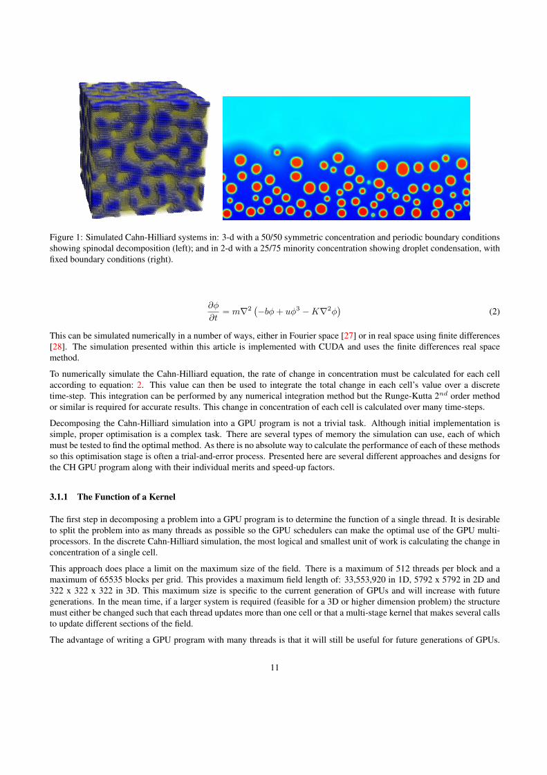
Figure 1: Simulated Cahn-Hilliard systems in: 3-d with a 50/50 symmetric concentration and periodic boundary conditionsshowing spinodal decomposition (left); and in 2-d with a 25/75 minority concentration showing droplet condensation, withfixed boundary conditions (right).

∂φ

∂t= m∇2

(−bφ + uφ3 −K∇2φ

)(2)

This can be simulated numerically in a number of ways, either in Fourier space [27] or in real space using finite differences[28]. The simulation presented within this article is implemented with CUDA and uses the finite differences real spacemethod.

To numerically simulate the Cahn-Hilliard equation, the rate of change in concentration must be calculated for each cellaccording to equation: 2. This value can then be used to integrate the total change in each cell’s value over a discretetime-step. This integration can be performed by any numerical integration method but the Runge-Kutta 2nd order methodor similar is required for accurate results. This change in concentration of each cell is calculated over many time-steps.

Decomposing the Cahn-Hilliard simulation into a GPU program is not a trivial task. Although initial implementation issimple, proper optimisation is a complex task. There are several types of memory the simulation can use, each of whichmust be tested to find the optimal method. As there is no absolute way to calculate the performance of each of these methodsso this optimisation stage is often a trial-and-error process. Presented here are several different approaches and designs forthe CH GPU program along with their individual merits and speed-up factors.

3.1.1 The Function of a Kernel

The first step in decomposing a problem into a GPU program is to determine the function of a single thread. It is desirableto split the problem into as many threads as possible so the GPU schedulers can make the optimal use of the GPU multi-processors. In the discrete Cahn-Hilliard simulation, the most logical and smallest unit of work is calculating the change inconcentration of a single cell.

This approach does place a limit on the maximum size of the field. There is a maximum of 512 threads per block and amaximum of 65535 blocks per grid. This provides a maximum field length of: 33,553,920 in 1D, 5792 x 5792 in 2D and322 x 322 x 322 in 3D. This maximum size is specific to the current generation of GPUs and will increase with futuregenerations. In the mean time, if a larger system is required (feasible for a 3D or higher dimension problem) the structuremust either be changed such that each thread updates more than one cell or that a multi-stage kernel that makes several callsto update different sections of the field.

The advantage of writing a GPU program with many threads is that it will still be useful for future generations of GPUs.

11

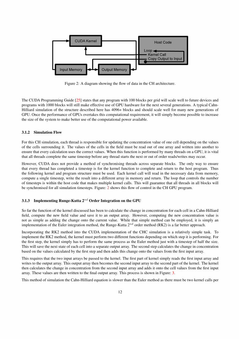
Figure 2: A diagram showing the flow of data in the CH architecture.

The CUDA Programming Guide [25] states that any program with 100 blocks per grid will scale well to future devices andprograms with 1000 blocks will still make effective use of GPU hardware for the next several generations. A typical Cahn-Hilliard simulation of the structure described here has 4096+ blocks and should scale well for many new generations ofGPU. Once the performance of GPUs overtakes this computational requirement, it will simply become possible to increasethe size of the system to make better use of the computational power available.

3.1.2 Simulation Flow

For this CH simulation, each thread is responsible for updating the concentration value of one cell depending on the valuesof the cells surrounding it. The values of the cells in the field must be read out of one array and written into another toensure that every calculation uses the correct values. When this function is performed by many threads on a GPU, it is vitalthat all threads complete the same timestep before any thread starts the next or out of order reads/writes may occur.

However, CUDA does not provide a method of synchronising threads across separate blocks. The only way to ensurethat every thread has completed a timestep is for the kernel function to complete and return to the host program. Thusthe following kernel and program structure must be used. Each kernel call will read in the necessary data from memory,compute a single timestep, write the result into a different array in memory and return. The loop that controls the numberof timesteps is within the host code that makes multiple kernel calls. This will guarantee that all threads in all blocks willbe synchronised for all simulation timesteps. Figure: 2 shows this flow of control in the CH GPU program.

3.1.3 Implementing Runge-Kutta 2nd Order Integration on the GPU

So far the function of the kernel discussed has been to calculate the change in concentration for each cell in a Cahn-Hilliardfield, compute the new field value and save it to an output array. However, computing the new concentration value isnot as simple as adding the change onto the current value. While that simple method can be employed, it is simply animplementation of the Euler integration method, the Runge-Kutta 2nd order method (RK2) is a far better approach.

Incorporating the RK2 method into the CUDA implementation of the CHC simulation is a relatively simple task. Toimplement the RK2 method, the kernel must perform two different functions depending on which step it is performing. Forthe first step, the kernel simply has to perform the same process as the Euler method just with a timestep of half the size.This will save the next state of each cell into a separate output array. The second step calculates the change in concentrationbased on the values calculated by the first step and then adds this change onto the values from the first input array.

This requires that the two input arrays be passed to the kernel. The first part of kernel simply reads the first input array andwrites to the output array. This output array then becomes the second input array to the second part of the kernel. The kernelthen calculates the change in concentration from the second input array and adds it onto the cell values from the first inputarray. These values are then written to the final output array. This process is shown in Figure: 3.

This method of simulation the Cahn-Hilliard equation is slower than the Euler method as there must be two kernel calls per

12

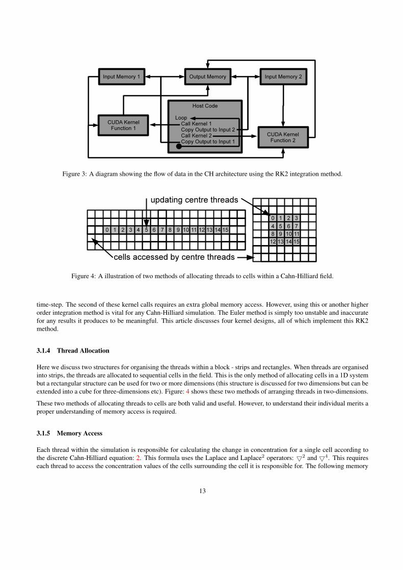
Figure 3: A diagram showing the flow of data in the CH architecture using the RK2 integration method.

Figure 4: A illustration of two methods of allocating threads to cells within a Cahn-Hilliard field.

time-step. The second of these kernel calls requires an extra global memory access. However, using this or another higherorder integration method is vital for any Cahn-Hilliard simulation. The Euler method is simply too unstable and inaccuratefor any results it produces to be meaningful. This article discusses four kernel designs, all of which implement this RK2method.

3.1.4 Thread Allocation

Here we discuss two structures for organising the threads within a block - strips and rectangles. When threads are organisedinto strips, the threads are allocated to sequential cells in the field. This is the only method of allocating cells in a 1D systembut a rectangular structure can be used for two or more dimensions (this structure is discussed for two dimensions but can beextended into a cube for three-dimensions etc). Figure: 4 shows these two methods of arranging threads in two-dimensions.

These two methods of allocating threads to cells are both valid and useful. However, to understand their individual merits aproper understanding of memory access is required.

3.1.5 Memory Access

Each thread within the simulation is responsible for calculating the change in concentration for a single cell according tothe discrete Cahn-Hilliard equation: 2. This formula uses the Laplace and Laplace2 operators: 52 and 54. This requireseach thread to access the concentration values of the cells surrounding the cell it is responsible for. The following memory

13

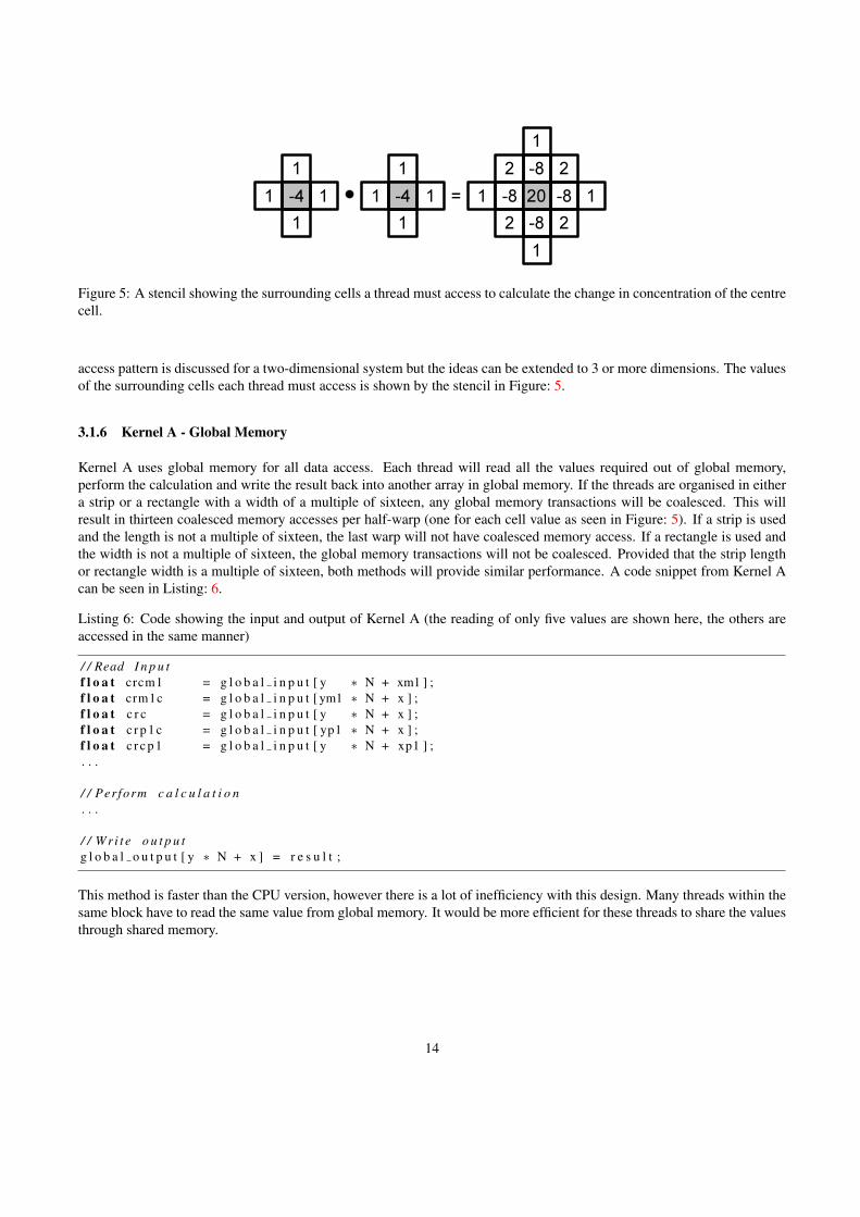
Figure 5: A stencil showing the surrounding cells a thread must access to calculate the change in concentration of the centrecell.

access pattern is discussed for a two-dimensional system but the ideas can be extended to 3 or more dimensions. The valuesof the surrounding cells each thread must access is shown by the stencil in Figure: 5.

3.1.6 Kernel A - Global Memory

Kernel A uses global memory for all data access. Each thread will read all the values required out of global memory,perform the calculation and write the result back into another array in global memory. If the threads are organised in eithera strip or a rectangle with a width of a multiple of sixteen, any global memory transactions will be coalesced. This willresult in thirteen coalesced memory accesses per half-warp (one for each cell value as seen in Figure: 5). If a strip is usedand the length is not a multiple of sixteen, the last warp will not have coalesced memory access. If a rectangle is used andthe width is not a multiple of sixteen, the global memory transactions will not be coalesced. Provided that the strip lengthor rectangle width is a multiple of sixteen, both methods will provide similar performance. A code snippet from Kernel Acan be seen in Listing: 6.

Listing 6: Code showing the input and output of Kernel A (the reading of only five values are shown here, the others areaccessed in the same manner)

/ / Read I n p u tf l o a t crcm1 = g l o b a l i n p u t [ y ∗ N + xm1 ] ;f l o a t crm1c = g l o b a l i n p u t [ ym1 ∗ N + x ] ;f l o a t c r c = g l o b a l i n p u t [ y ∗ N + x ] ;f l o a t c r p 1 c = g l o b a l i n p u t [ yp1 ∗ N + x ] ;f l o a t c r c p 1 = g l o b a l i n p u t [ y ∗ N + xp1 ] ;. . .

/ / Per form c a l c u l a t i o n. . .

/ / W r i t e o u t p u tg l o b a l o u t p u t [ y ∗ N + x ] = r e s u l t ;

This method is faster than the CPU version, however there is a lot of inefficiency with this design. Many threads within thesame block have to read the same value from global memory. It would be more efficient for these threads to share the valuesthrough shared memory.

14

3.1.7 Kernel B - Shared Memory

Kernel B uses shared memory to cache values read in from global memory. To make use of shared memory, each threadcan access one value from the global input memory and load it into shared memory. The surrounding threads in the sameblock can then access this shared data much faster than global memory. However, this raises the question of the optimumarrangement for threads to minimize the global data access.

If the threads are allocated to sequential cells in a strip then every thread must retrieve the values in the two cells aboveit and the two cells below it from global memory (see Figure: 5). They will only be able to use shared memory to accessvalues from the cells to the left and right. Threads that are arranged into a rectangle of cells can make more efficient useof shared memory. The threads within the centre of the grid will be able to access all neighbouring cell values from sharedmemory.

The problem with this is that the threads on the edge of the rectangle (or end of the strip) must perform more global memorytransactions than the other threads. This causes a branch in the kernel which can seriously impact the performance of theprogram. If any two threads within a warp take different branches, all the threads must perform the instructions for bothbranches but the appropriate threads are disabled for one of the branches. This causes a significant performance loss.

To eliminate this problem, the threads are rearranged such that there is a border of two surplus threads around the outsideof each thread grid that simply access the cell values from global memory and save them to shared memory. The downsideof this approach is that the thread grids must overlap resulting in more threads than there are cells. However, this approachis still faster than kernels with branches within them. The allocation of these threads to cells can be seen in Figure: 4 wherea thread is assigned to each empty surrounding cells. Listing: 7 shows how each kernel accesses the data.

Listing 7: Code showing the input and output of Kernel B (the reading of only five values are shown here, the others areaccessed in the same manner)

s h a r e d f l o a t s h a r e d d a t a [ BLOCK SIZE ∗ BLOCK SIZE ] ;

/ / Read i n t o sh ar ed memoryf l o a t c r c = g l o b a l i n p u t [ y ∗ N + x ] ;s h a r e d d a t a [ t y ∗ BLOCK SIZE + t x ] = c r c ;

s y n c t h r e a d s ( ) ;

/ / Work o u t i f t h i s t h r e a d i s a c a l c u l a t i n g t h r e a d or a b ord er t h r e a dbool w r i t e r = ( t x > 1) && ( t x < BLOCK SIZE − 2) && ( t y > 1) && ( t y < BLOCK SIZE − 2 ) ;

i f ( w r i t e r ) {/ / Read from sh ar ed memoryf l o a t crcm1 = s h a r e d d a t a [ t y ∗ BLOCK SIZE + txm1 ] ;f l o a t crm1c = s h a r e d d a t a [ tym1 ∗ BLOCK SIZE + t x ] ;f l o a t c r p 1 c = s h a r e d d a t a [ t yp1 ∗ BLOCK SIZE + t x ] ;f l o a t c r c p 1 = s h a r e d d a t a [ t y ∗ BLOCK SIZE + txp1 ] ;. . .



}

In order for this approach to work, the thread rectangle must be applied over the entire CH lattice such that each cell has oneupdating thread assigned to it. For this to work, the number of updating threads in the thread grid must divide the size of thelattice perfectly. A CH model lattice is normally a square grid with a size of some power of two. However, this is merely a

15

convention and in this case the size of the grid can have a serious impact on the performance of the program. As memoryaccess is fastest if all threads in a half-warp (16 threads) access sequential addresses in memory, it is advantageous if eachset of 16 threads in the grid are allocated to a single row in memory. It is also advantageous that the number of threadswithin a grid be a multiple of 32 as each warp will always be full and make the maximum use of the GPUs multiprocessors.

For this reason the optimal thread grid structure is a 16x16 block. This 16x16 block has a 12x12 block of updating threadswithin it where all global memory transactions are coalesced. It can be assumed that any useful CH simulation that requiresa GPU to execute in a reasonable amount of time will be larger than 12x12 thus this block structure will fit perfectly intoany lattice where the length is divisible by 12.

3.1.8 Kernel C - Texture Memory

Kernel C uses another option for accessing data, texture memory. Texture memory can provide several performance benefitsover global memory as input for the kernel [25]. When values are retrieved from texture memory, a global memory accessis only required if the value is not already stored within the texture cache. This effectively performs the caching effect ofusing shared memory but is performed by the GPU hardware rather than within the code itself. This also leaves the sharedmemory free for other purposes. The caching ability of textures can provide significant performance gains and can removethe often troublesome problem of arranging access to global memory to ensure coalesced access.

If the values required by the thread do not fit into the texture cache it will have to be constantly re-read from global memorywhich could seriously reduce the performance of the program. The actual size of the texture cache depends on the graphicscard however it should be at least 6 KB per multiprocessor(See PG appendix A.1.1). Easily capable of storing the memoryrequired for a 16x16 block of threads (maximum power of two square under the 512 limit). Listing: 8 shows the code fromKernel C that reads the data from a texture.

Listing 8: Code showing the input and output of Kernel C (the reading of only five values are shown here, the others areaccessed in the same manner)

t e x t u r e <f l o a t , 2 , cudaReadModeElementType> t e x t u r e i n p u t ;

/ / Read from t e x t u r e memoryf l o a t crcm1 = tex2D ( t e x t u r e i n p u t , xm1 , y ) ;f l o a t crm1c = tex2D ( t e x t u r e i n p u t , x , ym1 ) ;f l o a t c r c = tex2D ( t e x t u r e i n p u t , x , y ) ;f l o a t c r p 1 c = tex2D ( t e x t u r e i n p u t , x , yp1 ) ;f l o a t c r c p 1 = tex2D ( t e x t u r e i n p u t , xp1 , y ) ;. . .



There are some other advantages provided by texture memory such as the ability to automatically handle the boundaryconditions of a field. Cells on the edge of a field must either wrap around to the other side of the field or mirror back into thefield. Texture memory in a normalized access mode can automatically perform these boundary condition functions whichcan help to avoid expensive conditional statements that can cause threads within the same warp to take different branchesand can cause and significant impact on performance.

Another limitation of texture memory is that it can only support up to three dimensions. Any CH system that wishes tooperate on four or more dimensions can no longer easily make use of functions of texture memory. For texture memory to beused for any system that operates in more than three dimensions must create an array of three dimensional texture memory

16

segments. These memory segments would only be cached in three dimensions and would provide no caching ability in thefourth or higher dimension.

3.1.9 Kernel D - Texture and Shared Memory

For the sake of completeness, a fourth kernel has been implemented. This kernel uses texture and shared memory to readthe values from memory. The data is read out of texture memory into shared memory and then each thread accesses thevalues from shared memory. This is not particularly efficient because the data will be cached by the texture memory andthen again by the shared memory. However, it was implemented so that every method was properly explored. The code forthis kernel is shown in Listing: 9.

Listing 9: Code showing the input and output of Kernel D (the reading of only five values are shown here, the others areaccessed in the same manner)

t e x t u r e <f l o a t , 2 , cudaReadModeElementType> t e x t u r e i n p u t ;s h a r e d f l o a t s h a r e d d a t a [ BLOCK SIZE ∗ BLOCK SIZE ] ;

/ / Read i n t o sh ar ed memoryf l o a t c r c = tex2D ( t e x t u r e i n p u t , x , y ) ;s h a r e d d a t a [ t y ∗ BLOCK SIZE + t x ] = c r c ;

s y n c t h r e a d s ( ) ;

/ / Work o u t i f t h i s t h r e a d i s a c a l c u l a t i n g t h r e a d or a b ord er t h r e a dbool w r i t e r = ( t x > 1) && ( t x < BLOCK SIZE − 2) && ( t y > 1) && ( t y < BLOCK SIZE − 2 ) ;

i f ( w r i t e r ) {/ / Read from sh ar ed memoryf l o a t crcm1 = s h a r e d d a t a [ t y ∗ BLOCK SIZE + txm1 ] ;f l o a t crm1c = s h a r e d d a t a [ tym1 ∗ BLOCK SIZE + t x ] ;f l o a t c r p 1 c = s h a r e d d a t a [ t yp1 ∗ BLOCK SIZE + t x ] ;f l o a t c r c p 1 = s h a r e d d a t a [ t y ∗ BLOCK SIZE + txp1 ] ;. . .



}

One interesting problem encountered when implementing this kernel was the the size of the texture. Because the size of thefield must be divisible by the size of the inner rectangle (12x12 see Section: 3.1.7) the texture size must be a multiple of12. However, when normalized coordinates are used to provide automatic boundary condition handling (see Section: 3.1.8)the texture memory access no longer worked. It was found that normalised coordinates only worked correctly when thetexture size was a power of 2 (tested on an NVidia GeForce 8800 GTS). No documentation was found that warned of thisrequirement and the kernel had to be re-written to use non-normalised coordinates and hand-coded boundary conditionhandling.

3.1.10 Output from the Kernel

The only way for the threads to output the result of the calculation is by writing to an array in global memory. As the outputmust be performed via global memory, it is important that the output can be organised into coalesced write transactions.

17

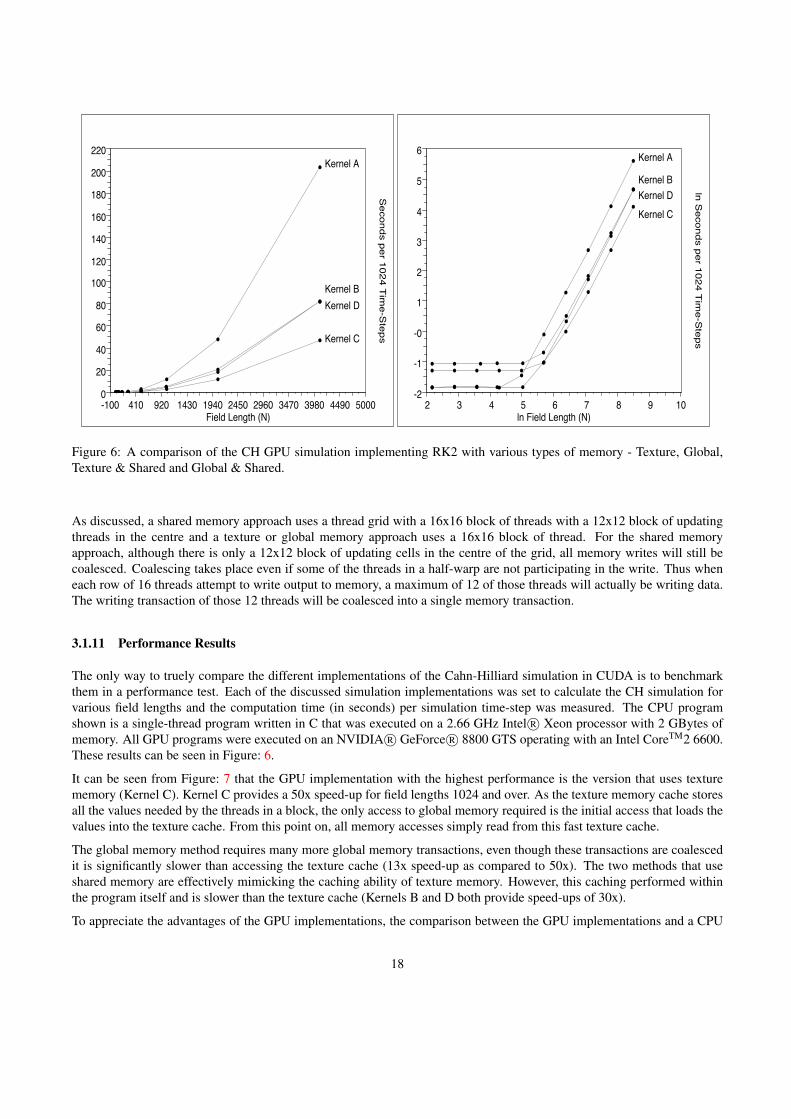
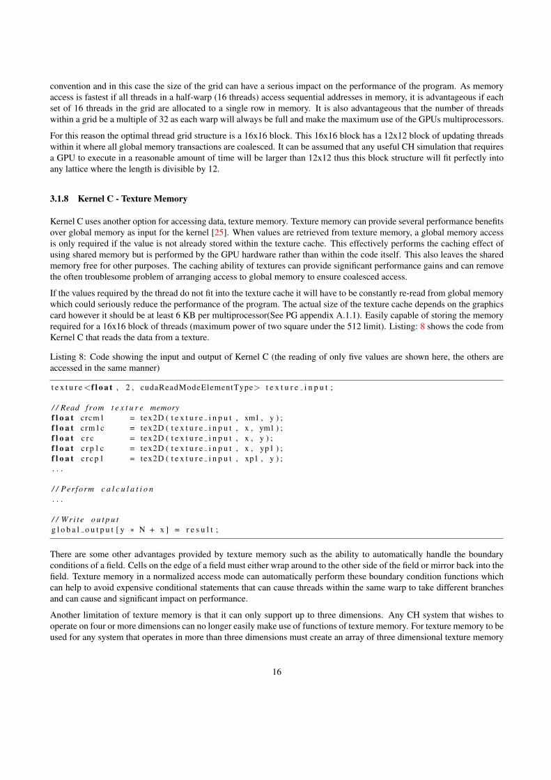
Figure 6: A comparison of the CH GPU simulation implementing RK2 with various types of memory - Texture, Global,Texture & Shared and Global & Shared.

As discussed, a shared memory approach uses a thread grid with a 16x16 block of threads with a 12x12 block of updatingthreads in the centre and a texture or global memory approach uses a 16x16 block of thread. For the shared memoryapproach, although there is only a 12x12 block of updating cells in the centre of the grid, all memory writes will still becoalesced. Coalescing takes place even if some of the threads in a half-warp are not participating in the write. Thus wheneach row of 16 threads attempt to write output to memory, a maximum of 12 of those threads will actually be writing data.The writing transaction of those 12 threads will be coalesced into a single memory transaction.

3.1.11 Performance Results

The only way to truely compare the different implementations of the Cahn-Hilliard simulation in CUDA is to benchmarkthem in a performance test. Each of the discussed simulation implementations was set to calculate the CH simulation forvarious field lengths and the computation time (in seconds) per simulation time-step was measured. The CPU programshown is a single-thread program written in C that was executed on a 2.66 GHz Intel R© Xeon processor with 2 GBytes ofmemory. All GPU programs were executed on an NVIDIA R© GeForce R© 8800 GTS operating with an Intel CoreTM2 6600.These results can be seen in Figure: 6.

It can be seen from Figure: 7 that the GPU implementation with the highest performance is the version that uses texturememory (Kernel C). Kernel C provides a 50x speed-up for field lengths 1024 and over. As the texture memory cache storesall the values needed by the threads in a block, the only access to global memory required is the initial access that loads thevalues into the texture cache. From this point on, all memory accesses simply read from this fast texture cache.

The global memory method requires many more global memory transactions, even though these transactions are coalescedit is significantly slower than accessing the texture cache (13x speed-up as compared to 50x). The two methods that useshared memory are effectively mimicking the caching ability of texture memory. However, this caching performed withinthe program itself and is slower than the texture cache (Kernels B and D both provide speed-ups of 30x).

To appreciate the advantages of the GPU implementations, the comparison between the GPU implementations and a CPU

18

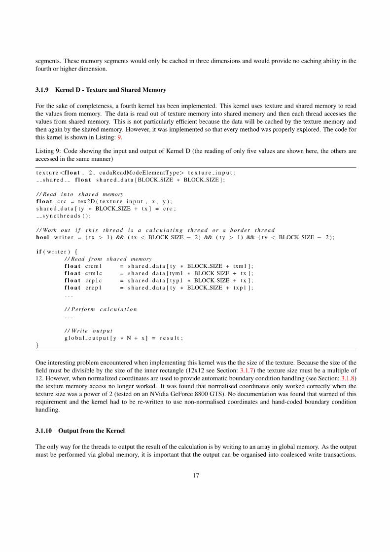
Figure 7: A comparison between GPU implementations and the CPU implementation.

version must be shown. As is expected, the GPU implementations of the simulation execute significantly faster for largefield lengths. As is common with parallel implementations, very small problems can be computed by a serial CPU faster asthere is no parallel overhead. However, as the field length (N) increases the problem becomes far more efficient to calculatein parallel using the GPU. As it is large simulations that provide the most meaningful results, GPU implementations ofsimulations have been proven to be extremely valuable.

4 GRAPH & NETWORK METRICS

Complex networks and their properties are being studied in many scientific fields to gain insights into topics as diverseas computer networks like the World-Wide Web [29], metabolic networks from biology [30, 31, 32], and social networks[33, 34, 35] investigating scientific collaborations [36, 37] or the structure of criminal organisations [38] to name but a few.These networks often consist of many thousands or even millions of nodes and many times more connections between thenodes. As diverse as the networks described in these articles may appear to be, they all share some common properties thatcan be used to categorise them. They all show characteristics of small-world networks, scale-free networks, or both. Thesetwo types of networks have therefore received much attention in the literature recently.

Networks are said to show the small-world effect if the mean geodesic distance (i.e. the shortest path between any twonodes) scales logarithmically or slower with the network size for fixed degree k [39]. They are highly clustered, like aregular graph, yet with small characteristic path length, like a random graph [40]. Scale-free networks have a power-lawdegree distribution for which the probability of a node having k links follows P (k) ∼ k−γ [41]. For example, in Price’spaper [42] concerning the number of references in scientific papers—one of the earliest published examples of scale-freenetworks—the exponent γ lies between 2.5 and 3.0 for the number of times a paper is cited.

Determining some of the computationally more expensive metrics, like the mean shortest paths between nodes [43,44], thevarious clustering coefficients [40,45,37,46], or the number of cycles/circuits of a specific length, which are commonly usedto study the properties of networks, can be infeasible on general purpose CPUs for such huge data structures. We utilise

19

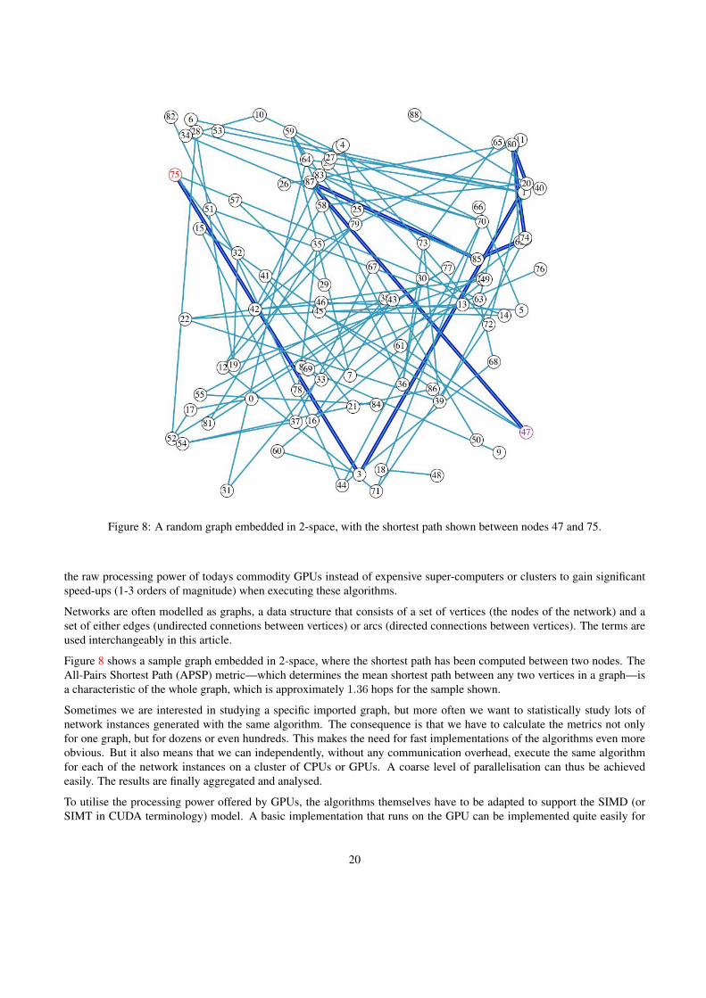
Figure 8: A random graph embedded in 2-space, with the shortest path shown between nodes 47 and 75.

the raw processing power of todays commodity GPUs instead of expensive super-computers or clusters to gain significantspeed-ups (1-3 orders of magnitude) when executing these algorithms.

Networks are often modelled as graphs, a data structure that consists of a set of vertices (the nodes of the network) and aset of either edges (undirected connetions between vertices) or arcs (directed connections between vertices). The terms areused interchangeably in this article.

Figure 8 shows a sample graph embedded in 2-space, where the shortest path has been computed between two nodes. TheAll-Pairs Shortest Path (APSP) metric—which determines the mean shortest path between any two vertices in a graph—isa characteristic of the whole graph, which is approximately 1.36 hops for the sample shown.

Sometimes we are interested in studying a specific imported graph, but more often we want to statistically study lots ofnetwork instances generated with the same algorithm. The consequence is that we have to calculate the metrics not onlyfor one graph, but for dozens or even hundreds. This makes the need for fast implementations of the algorithms even moreobvious. But it also means that we can independently, without any communication overhead, execute the same algorithmfor each of the network instances on a cluster of CPUs or GPUs. A coarse level of parallelisation can thus be achievedeasily. The results are finally aggregated and analysed.

To utilise the processing power offered by GPUs, the algorithms themselves have to be adapted to support the SIMD (orSIMT in CUDA terminology) model. A basic implementation that runs on the GPU can be implemented quite easily for

20

some of the graph algorithms that perform the same operation on every vertex or edge of the graph. However, optimisingthe implementation to make the most out of the available processing power can be quite challenging. It is necessary tothink about the optimal memory layout to reduce global memory transfers and make use of the available bandwidth throughcoalescing or texture fetches. If the threads have to communicate with each other at certain time steps, then it is a goodidea to arrange them in a way that allows them to use shared memory for most of the communication and only use globalmemory when absolutely necessary. Furthermore, divergent branches within warps caused by conditional execution orloops of different lengths should be avoided where possible, as every branch taken by at least one thread within the samewarp has to be serialised and executed by every thread of that warp.

The key problems that we had when implementing graph algorithms are related to the layout and access of global memoryand to branch divergence. The graph representation in memory and the patterns used to access the vertices and theirrespective edge lists have a large impact on the final performance as shown in the following sections. Graph algorithmsoften iterate over the neighbours lists of vertices to visit the nodes reacheable from each vertex. As there is no commonpattern of how vertices are connected with each other that is shared among different types of networks, it is often impossibleto completely avoid random memory accesses. Section 4.2 proposes different memory layouts that can be used to representgraphs on a CUDA-enabled device and explains why some provide better performance than others. Section 4.3 describesthe implementation of a specific graph algorithm and how it was optimised. Each optimisation step also states the respectiveperformance gains to show which changes have the largest impact. Finally, section 4.4 compares the CUDA implementationwith our implementation for the CPU.

4.1 Method & Approach

We implemented the APSP algorithm based on the approach described by Harish and Narayanan [47]. The algorithm isbasically a breadth-first search starting from a source vertex s with a frontier that expands outwards by one step in eachiteration (kernel call). This is done until all vertices that can be reached from s have been visited. The algorithm is invokedonce for every s ∈ V , where V is the set of vertices of a graph. We then optimised the implementation, tested various datastructures, different ways to access global memory and utilise shared memory, reduced data transfers between the host anddevice, and more. The following sections describe several of the optimisation techniques that were applied to the algorithm.

We use two different graph generation algorithms to generate the network instances that are used to test the GPU and CPUimplementations. For every tested network size N , 10 instances of each of the two network types are generated with thesame parameters (size, degree, etc). The execution times for the implementations are measured and the mean values of thetiming results are used to generate the graphs given in the following sections. For the CPU implementation, the standarddeviations from the mean values are calculated and displayed as error bars. The execution time of the GPU implementation,however, depends largely on the result value, as the breadth-first search from a source vertex s requires as many kernelcalls as the longest geodesic distance from s to any other vertex. Thus, networks with a high APSP value take much longerto process than networks with a small APSP value. An almost linear relationship exists for networks that are otherwiseequal. To accommodate for this fact, the timing results for the CUDA implementations are normalised before the standarddeviations used for the error bars are calculated. The formula used to normalise the values is:

Normalised time =(time in seconds)

APSP∗ (mean APSP) (3)

The first algorithm generates networks based on Watts’ α-model [48]. This is an algorithm that, depending on the providedparameters, generates a strongly clustered small-world network that may or may not be fully connected. Two differentparameter sets are used to generate the networks, both produce graphs that are always fully connected and strongly clustered.The networks created with the first parameter set (1) have a rather high mean shortest path length. A minimally connectedring substrate, in which every vertex has precisely two edges, is used to ensure that every vertex can be reached from everyother vertex. The second set of parameters (2) produces graphs with slightly lower clustering coefficients due to a higherrandomness of the connections, but with much lower mean shortest path lengths. As it does not use a substrate, the fullyconnectedness of the resulting graphs is not guaranteed by the algorithm, but rather through graph analysis after they were

21

generated. The degree of the resulting networks is k = 10 in both cases.

The second algorithm generates networks (3) based on the gradual growth and preferential attachment model published byBarabasi and Albert [41]. The graphs follow a power-law degree distribution, are always fully connected, and have a smallmean shortest path length. The degree of the resulting networks is k = 100.

4.2 Data Structures

A graph G = (V,E) with a set of V vertices and a set of E edges or arcs can be represented in a variety of ways. Figure 9illustrates a number of representations for directed graphs. While they can also be used to represent undirected graphs, theyare not very efficient, as an edge has to be represented by two arcs going in either direction. Thus, the information is storedtwice, increasing the required storage space and the risk of inconsistent data when one of the arcs gets lost. However, ouralgorithms have to be able to work with directed graphs. Therefore, they use data structures that are based on arcs and notedges.

Example (a) graphically shows the vertices and how they are connected with each other. This representation is often usedto visualise a network for humans, whereas the other representations are more likely to be used as data structures read andmodified by programs. The adjacency-matrix represenation (b) with its O(N2) memory usage wastes a lot of space if thegraph is sparse, but it allows to quickly determine if a specific arc exists. This is the reason why this representation iscommonly used in graph algorithms like the APSP algorithm. However, we avoid the identity-matrix representation for theGPU implementations due to the tighter memory limitations on graphics cards, thus making it possible to process largernetworks. The data structure illustrated in (c) is much more memory efficient for sparse graphs, since only existing arcs arestored. These three graph representations can commonly be found in the literature [49].

The data structure shown in (d) is similar to the one in (c), but—unless the neighbours-lists only contain a single element—itwastes even less space as it gets rid of the pointers required to point from one element of the linked lists to the next one.(e) is the most memory efficient data structure presented here. It merely requires O(E + V + 1) space. The adjacency-listlength of a vertex v is not stored explicitely, but it can easily be calculated with the index values stored in the elements vand v + 1 of the vertices array (vertices[v + 1] − vertices[v]). The vertices array is of length V + 1 = N + 1 to makethis work with the neighbours-list of the last vertex as well. The data structure shown in (f) improves the utilisation of theavailable memory bandwidth by using structs that can hold 4 integers as described in section 2.2.1 and listing 2, only thatthe length of the sub-lists is stored in the vertices array. Some space is wasted if the lengths of the adjacency-lists is not amultiple of 4.

The data structures (e) and even more so (f) are less commonly used by algorithms running on the CPU, but they turn outto be well suited for CUDA applications. They efficiently represent sparse graphs and in the case of (f) are specificallyoptimised for the way memory is accessed on the graphics card. These two data structures or slight variations of them areused in the implementations described in the following section. It should be noted, however, that they are not necessarilythe best choice when the kernels modify the graph structure.

Efficiently adding additional arcs or vertices to the graph from within a kernel is a challenge, as memory can only beallocated by the host and not by the kernels in CUDA. If the maximum degree is known and enough device memory isavailable to store a data structure of size N ∗ kmax, then allocating a one-dimensional array like in (e) may be a goodsolution. The second array used to point to the first index of each neighbours-list is not needed in this case, as the fixeddegree makes it easy to calculate it. If the maximum degree is not known, then a flexible data structure like the onedescribed in (c) with the maximum storage space available for the graph allocated in advance may be a good candidate.The best solution always depends on the particular problem and testing more than one data structure can sometimes yieldunexpected results.

22

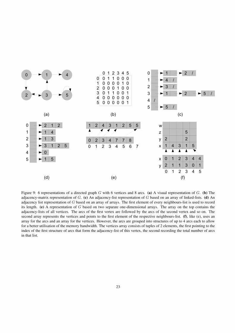
Figure 9: 6 representations of a directed graph G with 6 vertices and 8 arcs. (a) A visual representation of G. (b) Theadjacency-matrix representation of G. (c) An adjacency-list representation of G based on an array of linked-lists. (d) Anadjacency list representation of G based on an array of arrays. The first element of every neighbours-list is used to recordits length. (e) A representation of G based on two separate one-dimensional arrays. The array on the top contains theadjacency-lists of all vertices. The arcs of the first vertex are followed by the arcs of the second vertex and so on. Thesecond array represents the vertices and points to the first element of the respective neighbours-list. (f), like (e), uses anarray for the arcs and an array for the vertices. However, the arcs are grouped into structures of up to 4 arcs each to allowfor a better utilisation of the memory bandwidth. The vertices array consists of tuples of 2 elements, the first pointing to theindex of the first structure of arcs that form the adjacency-list of this vertex, the second recording the total number of arcsin that list.

23

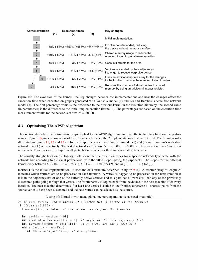
Figure 10: The evolution of the kernels, the key changes between the implementations and how the changes affect theexecution time when executed on graphs generated with Watts‘ α-model (1) and (2) and Barabasi’s scale-free networkmodel (3). The first percentage value is the difference to the previous kernel in the evolution hierarchy, the second value(in parantheses) is the difference to the initial implementation (kernel 1). The percentages are based on the execution timemeasurement results for the networks of size N = 30000.

4.3 Optimising The APSP Algorithm

This section describes the optimisation steps applied to the APSP algorithm and the effects that they have on the perfor-mance. Figure 10 gives an overview of the differences between the 7 implementations that were tested. The timing resultsillustrated in figures 11, 12 and 13 are for the graphs generated with Watts’ α-model (1) and (2) and Barabasi’s scale-freenetwork model (3) respectively. The tested networks are of size N = {1000, . . . , 30000}. The execution times t are givenin seconds. Error bars are displayed in all plots, but in some cases they are too small to be visible.

The roughly straight lines on the log-log plots show that the execution times for a specific network type scale with thenetwork size according to the usual power-laws, with the fitted slopes giving the exponents. The slopes for the differentkernels vary between ≈ (2.04 . . . 2.45) for (1), ≈ (1.49 . . . 1.94) for (2), and ≈ (1.51 . . . 1.71) for (3).

Kernel 1 is the initial implementation. It uses the data structure described in figure 9 (e). A frontier array of length Nindicates which vertices are to be processed in each iteration. A vertex is flagged to be processed in the next iteration ifit is in the adjacency-list of one of the currently active vertices and this path has a lower cost than any of the previouslydiscovered paths going through that vertex. The frontier array is copied back from the device to the host machine after everyiteration. The host machine determines if at least one vertex is active in the frontier, otherwise all shortest paths from thesource vertex s have been discovered and the next vertex can be selected as the source.

Listing 10: Kernel 1 with many global memory operations (coalesced or atomic).

/ / i f t h i s v e r t e x ( t i d = t h r e a d ID = v e r t e x ID ) i s a c t i v e i n t h e f r o n t i e ri f ( f r o n t i e r [ t i d ] ) {

f r o n t i e r [ t i d ] = f a l s e ; / / remove t h e v e r t e x from t h e f r o n t i e r

i n t a r c I d x = v e r t i c e s [ t i d ] ;i n t a rc sEnd = v e r t i c e s [ t i d + 1 ] ; / / b e g i n o f t h e n e x t a d j a c e n c y l i s ti n t newCostForNbrs = c o s t [ t i d ] + 1 ; / / e v e r y arc has a c o s t o f 1whi le ( a r c I d x < a rc sEnd ) {

i n t nbr = a r c s [ a r c I d x + + ] ; / / a n e i g h b o u r

24

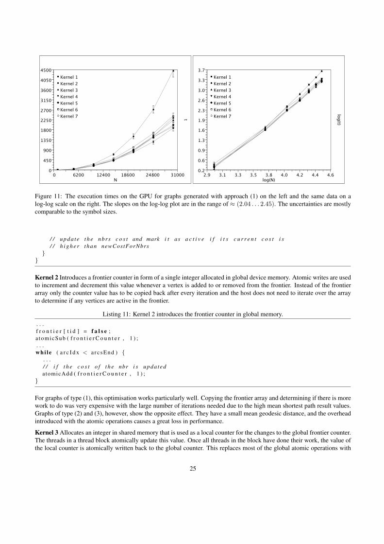
Figure 11: The execution times on the GPU for graphs generated with approach (1) on the left and the same data on alog-log scale on the right. The slopes on the log-log plot are in the range of ≈ (2.04 . . . 2.45). The uncertainties are mostlycomparable to the symbol sizes.

/ / up da t e t h e nbr s c o s t and mark i t as a c t i v e i f i t s c u r r e n t c o s t i s/ / h i g h e r than newCostForNbrs

}}

Kernel 2 Introduces a frontier counter in form of a single integer allocated in global device memory. Atomic writes are usedto increment and decrement this value whenever a vertex is added to or removed from the frontier. Instead of the frontierarray only the counter value has to be copied back after every iteration and the host does not need to iterate over the arrayto determine if any vertices are active in the frontier.

Listing 11: Kernel 2 introduces the frontier counter in global memory.

. . .f r o n t i e r [ t i d ] = f a l s e ;a tomicSub ( f r o n t i e r C o u n t e r , 1 ) ;. . .whi le ( a r c I d x < a rc sEnd ) {

. . ./ / i f t h e c o s t o f t h e nbr i s upda tedatomicAdd ( f r o n t i e r C o u n t e r , 1 ) ;

}

For graphs of type (1), this optimisation works particularly well. Copying the frontier array and determining if there is morework to do was very expensive with the large number of iterations needed due to the high mean shortest path result values.Graphs of type (2) and (3), however, show the opposite effect. They have a small mean geodesic distance, and the overheadintroduced with the atomic operations causes a great loss in performance.

Kernel 3 Allocates an integer in shared memory that is used as a local counter for the changes to the global frontier counter.The threads in a thread block atomically update this value. Once all threads in the block have done their work, the value ofthe local counter is atomically written back to the global counter. This replaces most of the global atomic operations with

25

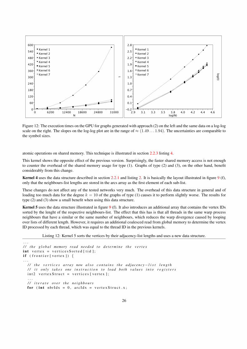
Figure 12: The execution times on the GPU for graphs generated with approach (2) on the left and the same data on a log-logscale on the right. The slopes on the log-log plot are in the range of ≈ (1.49 . . . 1.94). The uncertainties are comparable tothe symbol sizes.

atomic operations on shared memory. This technique is illustrated in section 2.2.3 listing 4.

This kernel shows the opposite effect of the previous version. Surprisingly, the faster shared memory access is not enoughto counter the overhead of the shared memory usage for type (1). Graphs of type (2) and (3), on the other hand, benefitconsiderably from this change.

Kernel 4 uses the data structure described in section 2.2.1 and listing 2. It is basically the layout illustrated in figure 9 (f),only that the neighbours-list lengths are stored in the arcs array as the first element of each sub-list.

These changes do not affect any of the tested networks very much. The overhead of this data structure in general and ofloading too much data for the degree k = 10 of the graphs of type (1) causes it to perform slightly worse. The results fortype (2) and (3) show a small benefit when using this data structure.

Kernel 5 uses the data structure illustrated in figure 9 (f). It also introduces an additional array that contains the vertex IDssorted by the lenght of the respective neighbours-list. The effect that this has is that all threads in the same warp processneighbours that have a similar or the same number of neighbours, which reduces the warp divergence caused by loopingover lists of different length. However, it requires an additional coalesced read from global memory to determine the vertexID processed by each thread, which was equal to the thread ID in the previous kernels.

Listing 12: Kernel 5 sorts the vertices by their adjacency-list lengths and uses a new data structure.

. . ./ / t h e g l o b a l memory read needed t o d e t e r m i n e t h e v e r t e xi n t v e r t e x = v e r t i c e s S o r t e d [ t i d ] ;i f ( f r o n t i e r [ v e r t e x ] ) {. . .

/ / t h e v e r t i c e s a r r a y now a l s o c o n t a i n s t h e ad jacency− l i s t l e n g t h/ / i t o n l y t a k e s one i n s t r u c t i o n t o load bo th v a l u e s i n t o r e g i s t e r si n t 2 v e r t e x S t r u c t = v e r t i c e s [ v e r t e x ] ;. . ./ / i t e r a t e over t h e n e i g h b o u r sf o r ( i n t n b r I d x = 0 , a r c I d x = v e r t e x S t r u c t . x ;

26

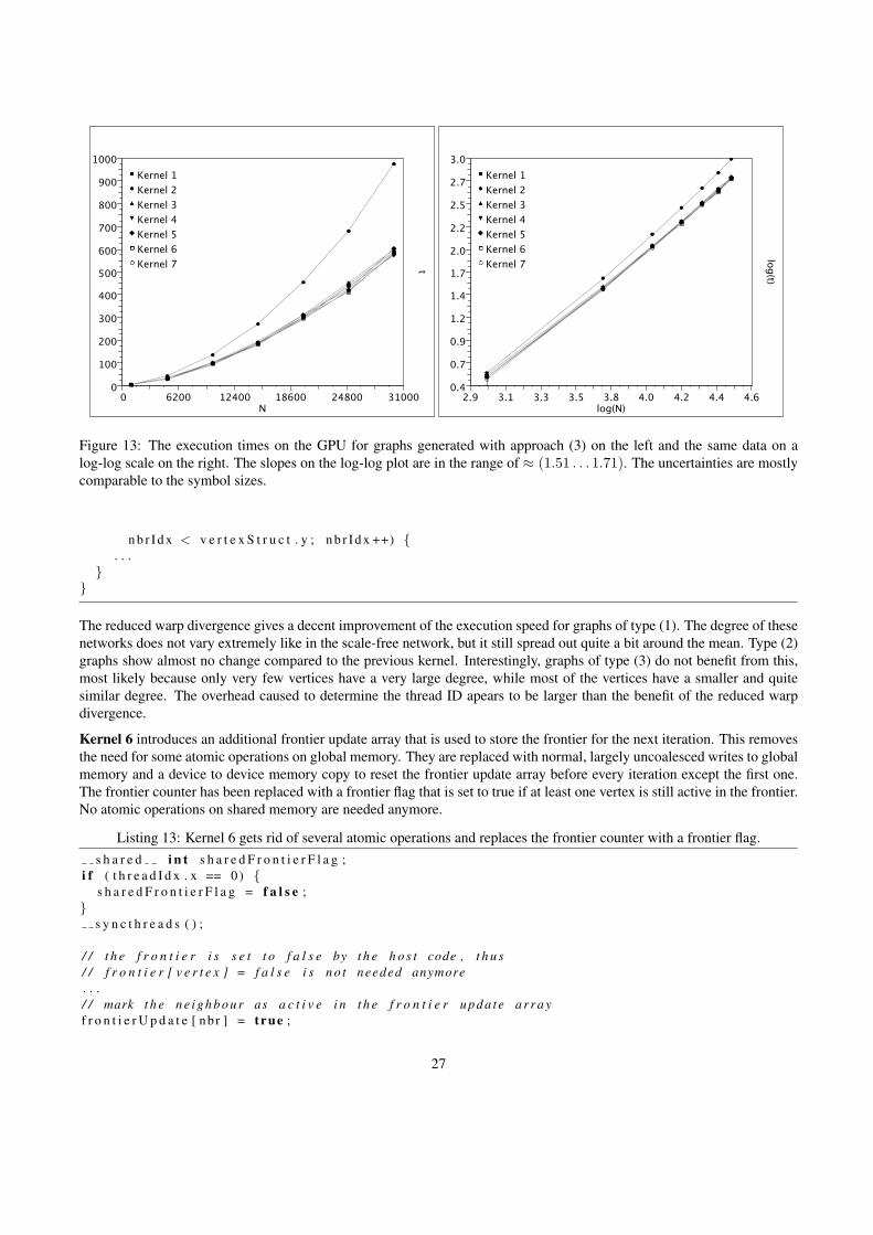
Figure 13: The execution times on the GPU for graphs generated with approach (3) on the left and the same data on alog-log scale on the right. The slopes on the log-log plot are in the range of ≈ (1.51 . . . 1.71). The uncertainties are mostlycomparable to the symbol sizes.

n b r I d x < v e r t e x S t r u c t . y ; n b r I d x ++) {. . .

}}

The reduced warp divergence gives a decent improvement of the execution speed for graphs of type (1). The degree of thesenetworks does not vary extremely like in the scale-free network, but it still spread out quite a bit around the mean. Type (2)graphs show almost no change compared to the previous kernel. Interestingly, graphs of type (3) do not benefit from this,most likely because only very few vertices have a very large degree, while most of the vertices have a smaller and quitesimilar degree. The overhead caused to determine the thread ID apears to be larger than the benefit of the reduced warpdivergence.

Kernel 6 introduces an additional frontier update array that is used to store the frontier for the next iteration. This removesthe need for some atomic operations on global memory. They are replaced with normal, largely uncoalesced writes to globalmemory and a device to device memory copy to reset the frontier update array before every iteration except the first one.The frontier counter has been replaced with a frontier flag that is set to true if at least one vertex is still active in the frontier.No atomic operations on shared memory are needed anymore.

Listing 13: Kernel 6 gets rid of several atomic operations and replaces the frontier counter with a frontier flag.s h a r e d i n t s h a r e d F r o n t i e r F l a g ;

i f ( t h r e a d I d x . x == 0) {s h a r e d F r o n t i e r F l a g = f a l s e ;

}s y n c t h r e a d s ( ) ;

/ / t h e f r o n t i e r i s s e t t o f a l s e by t h e h o s t code , t h u s/ / f r o n t i e r [ v e r t e x ] = f a l s e i s n o t needed anymore. . ./ / mark t h e n e i g h b o u r as a c t i v e i n t h e f r o n t i e r up da t e a r r a yf r o n t i e r U p d a t e [ nbr ] = t rue ;

27

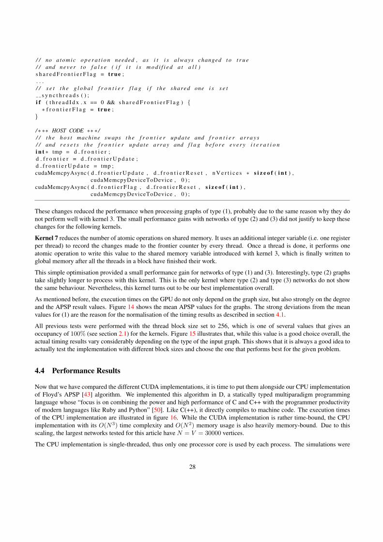
/ / no a t om ic o p e r a t i o n needed , as i t i s a lways changed t o t r u e/ / and n e v e r t o f a l s e ( i f i t i s m o d i f i e d a t a l l )s h a r e d F r o n t i e r F l a g = t rue ;. . ./ / s e t t h e g l o b a l f r o n t i e r f l a g i f t h e sh ar ed one i s s e t

s y n c t h r e a d s ( ) ;i f ( t h r e a d I d x . x == 0 && s h a r e d F r o n t i e r F l a g ) {∗ f r o n t i e r F l a g = t rue ;

}

/∗ ∗∗ HOST CODE ∗∗ ∗ // / t h e h o s t machine swaps t h e f r o n t i e r up da t e and f r o n t i e r a r r a y s/ / and r e s e t s t h e f r o n t i e r up da t e a r r a y and f l a g b e f o r e e v e r y i t e r a t i o ni n t ∗ tmp = d f r o n t i e r ;d f r o n t i e r = d f r o n t i e r U p d a t e ;d f r o n t i e r U p d a t e = tmp ;cudaMemcpyAsync ( d f r o n t i e r U p d a t e , d f r o n t i e r R e s e t , n V e r t i c e s ∗ s i z e o f ( i n t ) ,

cudaMemcpyDeviceToDevice , 0 ) ;cudaMemcpyAsync ( d f r o n t i e r F l a g , d f r o n t i e r R e s e t , s i z e o f ( i n t ) ,

cudaMemcpyDeviceToDevice , 0 ) ;

These changes reduced the performance when processing graphs of type (1), probably due to the same reason why they donot perform well with kernel 3. The small performance gains with networks of type (2) and (3) did not justify to keep thesechanges for the following kernels.

Kernel 7 reduces the number of atomic operations on shared memory. It uses an additional integer variable (i.e. one registerper thread) to record the changes made to the frontier counter by every thread. Once a thread is done, it performs oneatomic operation to write this value to the shared memory variable introduced with kernel 3, which is finally written toglobal memory after all the threads in a block have finished their work.

This simple optimisation provided a small performance gain for networks of type (1) and (3). Interestingly, type (2) graphstake slightly longer to process with this kernel. This is the only kernel where type (2) and type (3) networks do not showthe same behaviour. Nevertheless, this kernel turns out to be our best implementation overall.

As mentioned before, the execution times on the GPU do not only depend on the graph size, but also strongly on the degreeand the APSP result values. Figure 14 shows the mean APSP values for the graphs. The strong deviations from the meanvalues for (1) are the reason for the normalisation of the timing results as described in section 4.1.

All previous tests were performed with the thread block size set to 256, which is one of several values that gives anoccupancy of 100% (see section 2.1) for the kernels. Figure 15 illustrates that, while this value is a good choice overall, theactual timing results vary considerably depending on the type of the input graph. This shows that it is always a good idea toactually test the implementation with different block sizes and choose the one that performs best for the given problem.

4.4 Performance Results

Now that we have compared the different CUDA implementations, it is time to put them alongside our CPU implementationof Floyd’s APSP [43] algorithm. We implemented this algorithm in D, a statically typed multiparadigm programminglanguage whose “focus is on combining the power and high performance of C and C++ with the programmer productivityof modern languages like Ruby and Python” [50]. Like C(++), it directly compiles to machine code. The execution timesof the CPU implementation are illustrated in figure 16. While the CUDA implementation is rather time-bound, the CPUimplementation with its O(N3) time complexity and O(N2) memory usage is also heavily memory-bound. Due to thisscaling, the largest networks tested for this article have N = V = 30000 vertices.

The CPU implementation is single-threaded, thus only one processor core is used by each process. The simulations were

28

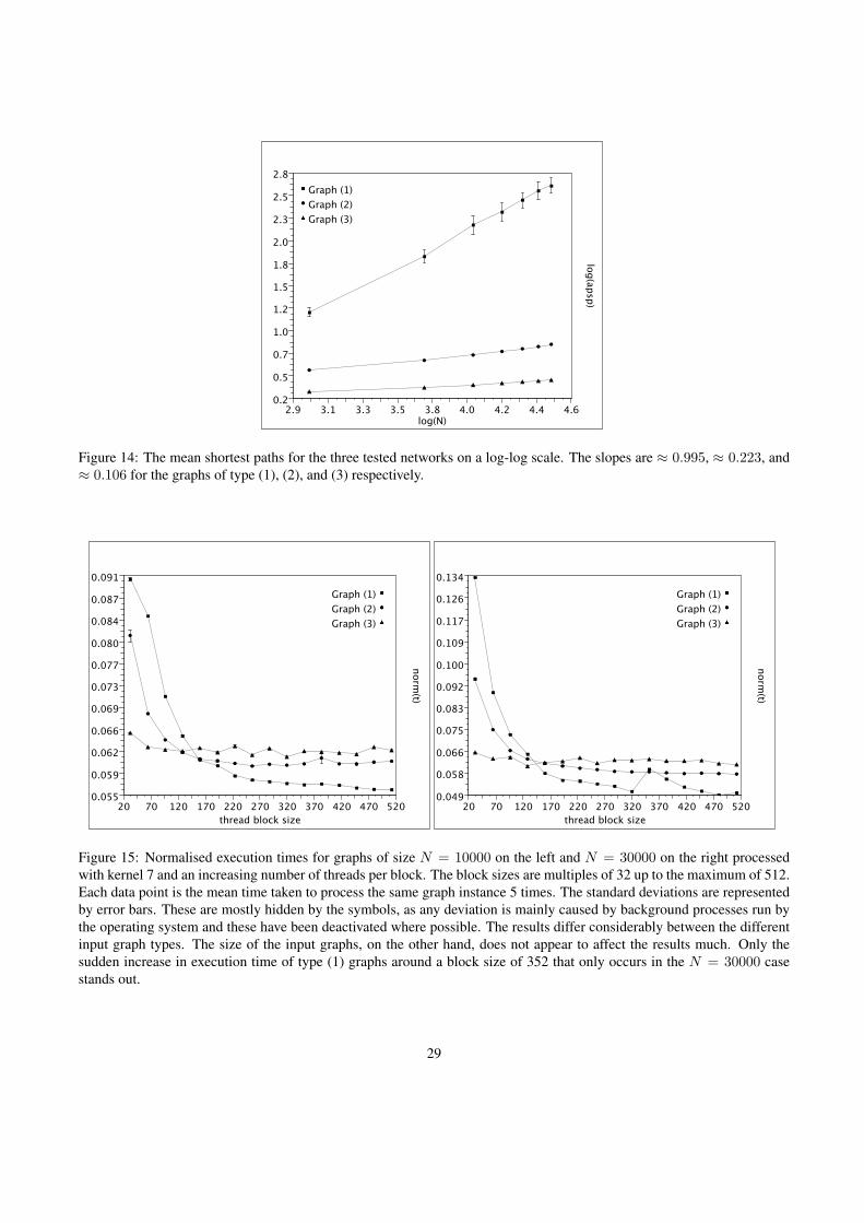
Figure 14: The mean shortest paths for the three tested networks on a log-log scale. The slopes are ≈ 0.995, ≈ 0.223, and≈ 0.106 for the graphs of type (1), (2), and (3) respectively.

Figure 15: Normalised execution times for graphs of size N = 10000 on the left and N = 30000 on the right processedwith kernel 7 and an increasing number of threads per block. The block sizes are multiples of 32 up to the maximum of 512.Each data point is the mean time taken to process the same graph instance 5 times. The standard deviations are representedby error bars. These are mostly hidden by the symbols, as any deviation is mainly caused by background processes run bythe operating system and these have been deactivated where possible. The results differ considerably between the differentinput graph types. The size of the input graphs, on the other hand, does not appear to affect the results much. Only thesudden increase in execution time of type (1) graphs around a block size of 352 that only occurs in the N = 30000 casestands out.

29

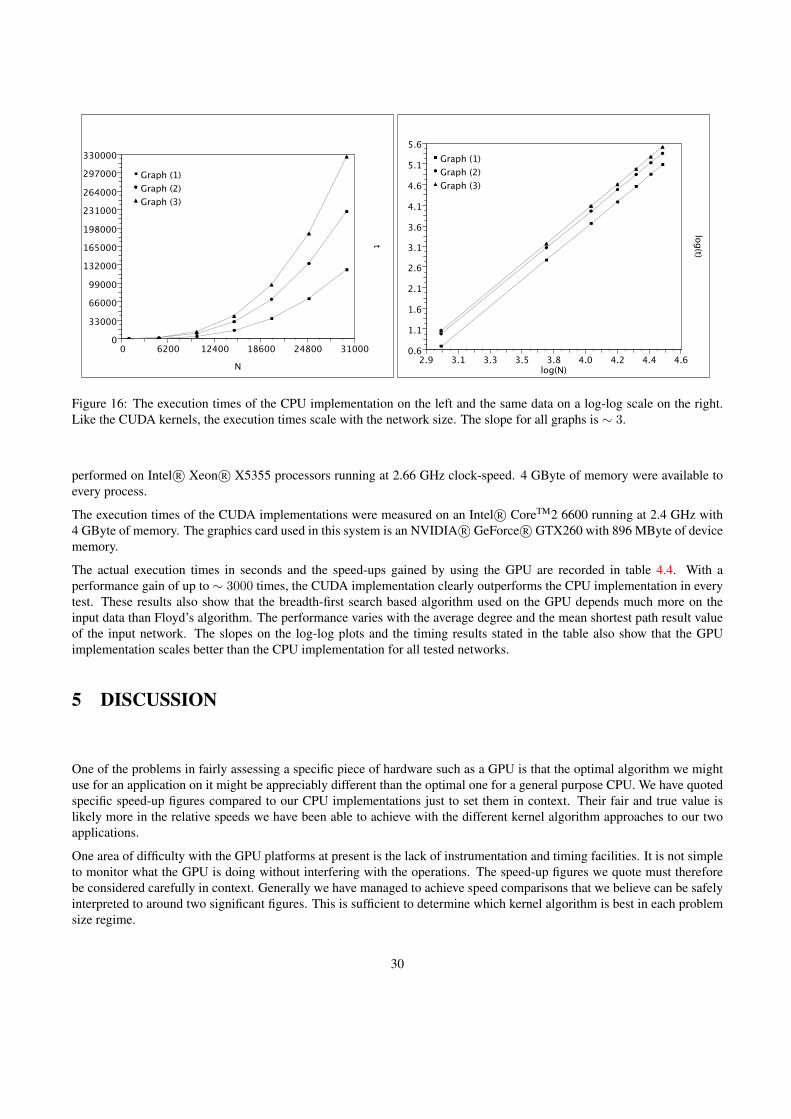
Figure 16: The execution times of the CPU implementation on the left and the same data on a log-log scale on the right.Like the CUDA kernels, the execution times scale with the network size. The slope for all graphs is ∼ 3.

performed on Intel R© Xeon R© X5355 processors running at 2.66 GHz clock-speed. 4 GByte of memory were available toevery process.

The execution times of the CUDA implementations were measured on an Intel R© CoreTM2 6600 running at 2.4 GHz with4 GByte of memory. The graphics card used in this system is an NVIDIA R© GeForce R© GTX260 with 896 MByte of devicememory.

The actual execution times in seconds and the speed-ups gained by using the GPU are recorded in table 4.4. With aperformance gain of up to ∼ 3000 times, the CUDA implementation clearly outperforms the CPU implementation in everytest. These results also show that the breadth-first search based algorithm used on the GPU depends much more on theinput data than Floyd’s algorithm. The performance varies with the average degree and the mean shortest path result valueof the input network. The slopes on the log-log plots and the timing results stated in the table also show that the GPUimplementation scales better than the CPU implementation for all tested networks.

5 DISCUSSION

One of the problems in fairly assessing a specific piece of hardware such as a GPU is that the optimal algorithm we mightuse for an application on it might be appreciably different than the optimal one for a general purpose CPU. We have quotedspecific speed-up figures compared to our CPU implementations just to set them in context. Their fair and true value islikely more in the relative speeds we have been able to achieve with the different kernel algorithm approaches to our twoapplications.

One area of difficulty with the GPU platforms at present is the lack of instrumentation and timing facilities. It is not simpleto monitor what the GPU is doing without interfering with the operations. The speed-up figures we quote must thereforebe considered carefully in context. Generally we have managed to achieve speed comparisons that we believe can be safelyinterpreted to around two significant figures. This is sufficient to determine which kernel algorithm is best in each problemsize regime.

30

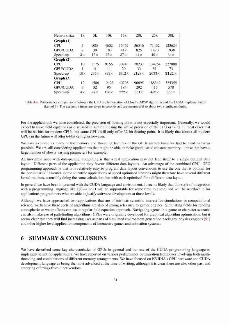
Network size 1k 5k 10k 15k 20k 25k 30kGraph (1)CPU 5 585 4602 15467 36546 71462 123624GPU/CUDA 2 39 183 419 825 1470 1938Speed-up 3× 15× 25× 37× 44× 49× 64×Graph (2)CPU 10 1175 9166 30243 70237 134264 227808GPU/CUDA 1 4 11 20 33 51 73Speed-up 10× 294× 833× 1512× 2128× 2633× 3121×Graph (3)CPU 12 1506 12123 40798 96695 188349 325355GPU/CUDA 3 32 95 184 292 417 578Speed-up 4× 47× 128× 222× 331× 452× 563×

Table 4.4. Performance comparisons between the CPU implementation of Floyd’s APSP algorithm and the CUDA implementation(kernel 7). The execution times are given in seconds and are meaningful to about two significant digits.

For the applications we have considered, the precision of floating point is not especially important. Generally, we wouldexpect to solve field equations as discussed in section 3 using the native precision of the CPU or GPU. In most cases thatwill be 64-bits for modern CPUs, but some GPUs still only offer 32-bit floating point. It is likely that almost all modernGPUs in the future will offer 64-bit or higher however.

We have explored as many of the memory and threading features of the GPUs architectures we had to hand as far aspossible. We are still considering applications that might be able to make good use of constant memory – those that have alarge number of slowly varying parameters for example.

An inevitable issue with data-parallel computing is that a real application may not lend itself to a single optimal datalayout. Different parts of the application may favour different data layouts. An advantage of the combined CPU+GPUprogramming approach is that is is relatively easy to program data layout conversions to use the one that is optimal forthe particular GPU kernel. Some scientific applications or speed optimised libraries might therefore have several differentkernel routines, ostensibly doing the same calculation, but with each optimised for a different data layout.

In general we have been impressed with the CUDA language and environment. It seems likely that this style of integrationwith a programming language like C/C++ or D will be supportable for some time to come, and will be worthwhile forapplications programmers who are able to justify software development at those levels.

Although we have approached two applications that are of intrinsic scientific interest for simulations in computationalscience, we believe these sorts of algorithms are also of strong relevance to games engines. Simulating fields for rendingatmospheric or water effects can use a regular field equation approach. Navigating agents in a game or character scenariocan also make use of path-finding algorithms. GPUs were originally developed for graphical algorithm optimisation, but itseems clear that they will find increasing uses as parts of simulated environment generation packages, physics engines [51]and other higher level application components of interactive games and animation systems.

6 SUMMARY & CONCLUSIONS

We have described some key characteristics of GPUs in general and our use of the CUDA programming language toimplement scientific applications. We have reported on various performance optimisation techniques involving both multi-threading and combinations of different memory arrangements. We have focused on NVIDIA’s GPU hardware and CUDAdevelopment language as being the most advanced at the time of writing, although it is clear there are also other past andemerging offerings from other vendors.

31

One specific regular-mesh application we investigated, used a finite-difference solver for a partial differential field equationsuch as the Cahn-Hilliard system. Not surprisingly, we found that a parallel geometric decomposition involving a large num-ber of parallel threads that execute independently performed well on the GPUs. However less obviously, the performancewas also heavily dependent on how effectively we used the different sorts of memory available on the GPU. We showed thata sensible use of fast local texture memory was critical to achieving the most dramatic performance improvements.

We also investigated graph and network applications as typified by computation of the all-pairs, shortest-path metric onvarious sorts of scale-free and other graph instances. These algorithms are less obviously parallelisable, but we obtainedsignificant performance speed-ups again from arranging the algorithm so that it could best exploit a multi-threaded ar-chitecture such as the particular GPUs that we used. The correct approach was less obvious for these problems and weexperimented with several different parallelisation techniques. We found that it was possible to achieve a very significantspeed-up over a typical CPU by having the application’s network data suitably arranged in the GPU’s fast and local memory.

This effect is reminiscent of the super-linear speed-ups commonly reported in the late 1980’s when just having a multi-processor computer with more memory overall than was typically found on a single-processor system, allowed applicationsto avoid slow memory or very slow disk swapping. Similar effects were not uncommon in the early 1990s when sophis-ticated multi-level caches became prevalent in CPUs. Optimising compilers can make some headway in cache predictionoptimisations, and it is likely that this is easier to do for a regular mesh problem than for an arbitrary graph problem. Thislikely explains why we have been able to hand optimise a more dramatic speed-up (relative to typical CPU performance)for graph problems in our hand-optimised GPU CUDA code than we could with the regular mesh application.

We found the GPU architectures and their available features very interesting to use, and we observe that a language likeCUDA makes these ideas much more accessible to applications programmers than has previously been the case. Neverthe-less parallel computing on GPUs remains non-trivial to use. Not all applications programmers will find the performancegains worth the additional thinking and development effort necessary to produce an optimised and maintainable code. Theeffort will likely continue to be worthwhile for game developers and those interested in fast and cheap scientific computingresources, like ourselves.

The economics of the games industry seems to have been the main driver for the low cost and wide availability of GPUs. Itis interesting that data-parallel computing is once again attracting attention and development effort as the ideas it embodiesbecome available in a useful and relatively easily exploitable manner on affordable hardware. We speculate that in the futuremore data-parallel concepts, as used now in GPUs, will be absorbed onto future multi-core CPUs.

It remains to be seen however, exactly what tool developments will be needed to ensure these features can be widelyused by applications programmers. It is likely that sophisticated scientific libraries using data-parallel ideas will be portedto such future chips. It is still not yet clear how many of the data-parallel ideas can be made available as standard ingeneral-purpose language compilers. Modern high-level languages such as Fortress [52] may be able to embed run-timelibrary components that have been optimised for such hardware. In the meantime, other mid level approaches such as usingscripting language bindings such as PyCUDA [53] may be a worthwhile approach. There does still seem to be a need forgeneral-purpose programming languages that better integrate data-parallel ideas. There will also continue to be interestingresearch opportunities on tradeoff analyses to determine what balance of computation is best located on a CPU and itsco-GPU(s).

Acknowledgments

It is a pleasure to thank C.H. Ling, I.A. Bond and C.J. Scogings for helpful discussions on GPUs and on scientific program-ming.

32

References

[1] Fox GC, Williams RD, Messina PC. Parallel Computing Works! Morgan Kaufmann Publishers, Inc., 1994. ISBN1-55860-253-4.

[2] Wilding N, Trew A, Hawick K, Pawley G. Scientific modeling with massively parallel SIMD computers. Proceedingsof the IEEE Apr 1991; 79(4):574–585, doi:10.1109/5.92050.

[3] Hillis WD. The Connection Machine. MIT Press, 1985.

[4] Johnsson SL. Data parallel supercomputing. Preprint YALEU/DCS/TR-741, Yale University, New Haven, CT 06520sep 1989. The use of Parallel Procesors in Meteorology, Pub. Springer-Verlag.

[5] Yau HW, Fox GC, Hawick KA. Evaluation of High Performance Fortran through applications kernels. Proc. HighPerformance Computing and Networking 1997, 1997.

[6] Hawick KA, Havlak P. High performance Fortran motivating applications and user feedback. Technical Report NPACTechnical Report SCCS-692, Northeast Parallel Architectures Center January 1995.

[7] Fox G. Fortran D as a portable software system for parallel computers jun 1991. Center for Research on ParallelComputation, Rice University, PO Box 1892, Houston, Texas, TX 77251-1892, CRPC-TR91128.

[8] Chapman B, Mehrotra P, Zima H. Vienna Fortran - a Fortran language extension for distributed memory multiproces-sors. ICASE Interim Report 91-72, Institute for Computer Applications in Science and Engineering, NASA, LangleyResearch Center, Hampton, Virginia 23665-5225 sep 1991.

[9] Bozkus Z, Choudhary A, Fox GC, Haupt T, Ranka S. Fortran 90D/HPF compiler for distributed-memory MIMDcomputers: design, implementation, and performance results. Proc. Supercomputing ’93, Portland, OR, 1993; 351.

[10] Bogucz EA, Fox GC, Haupt T, Hawick KA, Ranka S. Preliminary evaluation of high-performance Fortran as a lan-guage for computational fluid dynamics. Proc. AIAA Fluid Dynamics Conf, AIAA 94-2262, Colorado Springs, 1994.

[11] Pacheco PS. Parallel Programming with MPI. Morgan Kaufmann Publishers Inc., 1996.

[12] Chandra R, Dagum L, Kohr D, Menon R, Maydan D, McDonald J. Parallel Programming in OpenMP. Morgan Kauf-mann Publishers Inc., 2001.

[13] Fatahalian K, Houston M. A Closer Look at GPUs. Communications of the ACM October 2008; 51(10):50–57.

[14] Owens JD, Luebke D, Govindaraju N, Harris M, Kruger J, Lefohn AE, Purcell T. A survey of general-purpose com-putation on graphics hardware. Eurographics 2005, State of the Art Reports, 2005; 21–51.

[15] Langdon W, Banzhaf W. A SIMD Interpreter for Genetic Programming on GPU Graphics Cards. Proc. EuroGP, vol.LNCS 4971, O’Neill M, Vanneschi L, Gustafson S, Alcazar AE, Falco ID, Cioppa AD, Tarantino E (eds.), 2008;73–85.

[16] Messmer P, Mullowney PJ, Granger BE. GPULib: GPU computing in high-level languages. Computing in Science &Engineering September/October 2008; 10(5):70–73.

[17] Nickolls J, Buck I, Garland M, Skadron K. Scalable parallel programming with CUDA. ACM Queue March/April2008; 6(2):40–53.

[18] Buck I, Foley T, Horn D, Sugerman J, Fatahalian K, Houston M, Hanrahan P. Brook for GPUs: stream computing ongraphics hardware. ACM Trans. Graph. 2004; 23(3):777–786, doi:http://doi.acm.org/10.1145/1015706.1015800.

[19] AMD. ATI CTM Guide 2006.

[20] McCool M, Toit SD. Metaprogramming GPUs with Sh. A K Peters, Ltd., 2004.

33

[21] Khronos Group. OpenCL 2008. URL http://www.khronos.org/opencl/.

[22] Playne DP, Gerdelan AP, Leist A, Scogings CJ, Hawick KA. Simulation modelling and visualisation: Toolkits forbuilding artificial worlds. Research Letters in the Information and Mathematical Sciences 2008; 12:25–50.

[23] Stock MJ, Gharakhani A. Toward efficient GPU-accelerated N-body simulations. in 46th AIAA Aerospace SciencesMeeting and Exhibit, AIAA 2008-608, 2008.

[24] Kavanagh GD, Lewis MC, Massingill BL. GPGPU planetary simulations with CUDA. Proceedings of the 2008 Inter-national Conference on Scientific Computing, 2008.

[25] NVIDIA R© Corporation. CUDATM 2.0 Programming Guide 2008. URL http://www.nvidia.com/, last ac-cessed November 2008.

[26] Cahn JW, Hilliard JE. Free Energy of a Nonuniform System. I. Interfacial Free Energy. The Journal of ChemicalPhysics 1958; 28(2):258–267.

[27] Chen LQ, Shen J. Applications of semi-implicit Fourier-spectral method to phase field equations. Computer PhysicsCommunications 1998; 108:147–158.

[28] Hawick KA, Playne DP. Modelling and visualizing the Cahn-Hilliard-Cook equation. Proceedings of 2008 Interna-tional Conference on Modeling, Simulation and Visualization Methods (MSV’08), Las Vegas, Nevada, 2008.

[29] Albert R, Jeong H, Barabsi AL. Diameter of the World-Wide Web. Nature September 1999; 401(6749):130–131.

[30] Jeong H, Tombor B, Albert R, Oltvai Z, Barabsi AL. The large-scale organization of metabolic networks. NatureOctober 2000; 407(6804):651–654.

[31] Fell DA, Wagner A. The small world of metabolism. Nature Biotechnology November 2000; 18(11):1121–1122.

[32] Wagner A, Fell DA. The small world inside large metabolic networks. Proceedings of the Royal Society B September2001; 268(1478):1803–1810.

[33] Milgram S. The Small-World Problem. Psychology Today 1967; 1:61–67.

[34] Liljeros F, Edling C, Amaral L, Stanley H, Aberg Y. The web of human sexual contacts. Nature June 2001;411(6840):907–908.

[35] Liben-Nowell D, Kleinberg J. Tracing information flow on a global scale using Internet chain-letter data. PNAS March2008; 105(12):4633–4638.

[36] Newman MEJ. The structure of scientific collaboration networks. PNAS January 2001; 98(2):404–409.

[37] Newman MEJ. Ego-centered networks and the ripple effect. Social Networks January 2003; 25(1):83–95.

[38] Xu J, Chen H. The Topology of Dark Networks. Communications of the ACM October 2008; 51(10):58–65, doi:http://doi.acm.org/10.1145/1400181.1400198.

[39] Newman MEJ. The Structure and Function of Complex Networks. SIAM Review June 2003; 45(2):167–256.

[40] Watts DJ, Strogatz SH. Collective dynamics of ‘small-world’ networks. Nature June 1998; 393(6684):440–442.

[41] Barabsi AL, Albert R. Emergence of scaling in random networks. Science October 1999; 286(5439):509–512.

[42] Price DJd. Networks of Scientific Papers. Science July 1965; 149(3683):510–515, doi:10.1126/science.149.3683.

[43] Floyd RW. Algorithm 97: Shortest Path. Communications of the ACM 1962; 5(6):345.

[44] Dijkstra E. A Note on Two Problems in Connexion with Graphs. Numerische Mathematik 1959; 1(1):269–271.

34

http://www.khronos.org/opencl/

http://www.nvidia.com/

[45] Newman MEJ, Strogatz SH, Watts DJ. Random graphs with arbitrary degree distributions and their applications.Physical Review E July 2001; 64(2):026 118, doi:10.1103/PhysRevE.64.026118.

[46] Abdo AH, de Moura APS. Clustering as a measure of the local topology of networks. Technical Report, Universidadede Sao Paulo, University of Aberdeen February 2008. URL http://arxiv.org/abs/physics/0605235v4.

[47] Harish P, Narayanan P. Accelerating large graph algorithms on the GPU using CUDA. High Performance Computing- HiPC 2007: 14th International Conference, Proceedings, vol. 4873, Aluru S, Parashar M, Badrinath R, Prasanna V(eds.), Springer-Verlag: Goa, India, 2007; 197–208.

[48] Watts DJ. Small Worlds: The Structure of Networks between Order and Randomness. Princeton University Press,1999.

[49] Cormen TH, Leiserson CE, Rivest RL, Stein C. Introduction To Algorithms. 2 edn., MIT Press, 2001.

[50] Bright W. D Programming Language. Digital Mars 2008. URL www.digitalmars.com/d/.

[51] Conger D, LaMothe A. Physics Modeling for Game Programmers. Thompson, 2004.

[52] Allen E, Chase D, Flood C, Luchangco V, Maessen JW, Ryu S, Steele Jr GL. Project Fortress - a multicore languagefor multicore processors. Linux Magazine September 2007; :38–43.

[53] Klockner A. PyCUDA v0.91.1 documentation December 2008. URL http://documen.tician.de/pycuda/.

35

http://arxiv.org/abs/physics/0605235v4

www.digitalmars.com/d/

http://documen.tician.de/pycuda/

Technical Report CSTN-065 Exploiting Graphical Processing ...

Documents

Transcript of Technical Report CSTN-065 Exploiting Graphical Processing ...