Fundamentals of Rietveld Refinement II. Refinement of a Single Phase

TECHNICAL REFERENCE
Alan A Coelho
Bruker–AXS
http://www.bruker-axs.de/
September 8, 2016
Peak fitting, Pawley & Le Bail refinement, Rietveld refinement, PDF refinement, Magnetic structures, CW Neutron refinement, TOF refinement, Stacking faults, Laue refinement, Indexing, Charge flipping, Structure solution, Penalties, Restraints.
TOPAS-Academic - 6, Introduction, 2015 1
1 Introduction
Contents
1 INTRODUCTION .................................................................................................................... 6
1.1 CONVENTIONS ................................................................................................................................................ 6 1.2 INPUT FILE EXAMPLE (INP FORMAT) .................................................................................................................... 6 1.3 TEST EXAMPLES ............................................................................................................................................... 7
1.3.1 TC-INPS.BAT and the aac$ macro ....................................................................................................... 7 1.4 TOPAS IS NOW 64 BIT ..................................................................................................................................... 8
1.4.1 Limiting Memory Usage – MaxMem.TXT ........................................................................................... 8
2 PARAMETERS ....................................................................................................................... 9
2.1 WHEN IS A PARAMETER REFINED ........................................................................................................................ 9 2.2 USER DEFINED PARAMETERS - THE PRM KEYWORD ................................................................................................. 9 2.3 PARAMETER CONSTRAINTS .............................................................................................................................. 10 2.4 THE LOCAL KEYWORD ..................................................................................................................................... 11 2.5 REPORTING ON EQUATION VALUES .................................................................................................................... 11 2.6 NAMING OF EQUATIONS ................................................................................................................................. 12 2.7 EXISTING_PRM .............................................................................................................................................. 12 2.8 DUMMY AND DUMMY_PRM KEYWORDS ............................................................................................................. 13 2.9 PARAMETER ERRORS AND CORRELATION MATRIX ................................................................................................. 13 2.10 DEFAULT PARAMETER LIMITS AND LIMIT_MIN / LIMIT_MAX ............................................................................ 13 2.11 RESERVED PARAMETER NAMES ......................................................................................................................... 14 2.12 VAL AND CHANGE RESERVED PARAMETER NAMES ................................................................................................ 16 2.13 USING LOCAL TO ASSIST IN USING “FOR … {}” LOOPS ............................................................................................ 16 2.14 OUT_DEPENDENCES AND OUT_DEPENDENCES_FOR .............................................................................................. 17 2.15 THE NUM_RUNS KEYWORD AND PREPROCESSOR SPECIFICS .................................................................................... 18
2.15.1 Reserved macro Names .................................................................................................................... 20 2.15.2 The #list directive – creating arrays of macros ................................................................................. 20 2.15.3 The File_Variable and File_Variables macro .................................................................................... 21
3 EQUATION OPERATORS AND FUNCTIONS ........................................................................... 23
3.1 'IF' AND NESTED 'IF' STATEMENTS ..................................................................................................................... 25 3.2 FLOATING POINT EXCEPTIONS ........................................................................................................................... 25
4 THE MINIMIZATION ROUTINES ........................................................................................... 26
4.1 THE MARQUARDT METHOD ............................................................................................................................. 27 4.2 APPROXIMATING THE A MATRIX - THE BFGS METHOD .......................................................................................... 28 4.3 LINE MINIMIZATION AND PARAMETER EXTRAPOLATION ......................................................................................... 28 4.4 THE CONJUGATE GRADIENT SOLUTION METHOD ................................................................................................. 28 4.5 RESTRAINTS AND PENALTIES ............................................................................................................................ 29 4.6 MINIMIZING ON PENALTIES ONLY ...................................................................................................................... 30 4.7 SAVED REFINED VALUES AND SAVE_BEST_CHI2.................................................................................................... 30 4.8 ERROR CALCULATION ..................................................................................................................................... 31 4.9 ERROR DETERMINATION USING SVD ................................................................................................................. 31 4.10 ERROR PROPAGATION USING PRM_WITH_ERROR ................................................................................................ 32 4.11 SIMULATED ANNEALING ADAPTIVE STEP SIZE ....................................................................................................... 32 4.12 REFINING ON AN ARBITRARY CHI
2 ..................................................................................................................... 32
4.13 INFORMING ON UNREFINED PARAMETERS ........................................................................................................... 33 4.14 SUMMARY, ITERATION AND REFINEMENT CYCLE .................................................................................................. 34 4.15 QUICK_REFINE AND COMPUTATIONAL ISSUES ...................................................................................................... 34 4.16 AUTO_T AND RANDOMIZE_ON_ERRORS ............................................................................................................ 35 4.17 CRITERIA OF FIT ............................................................................................................................................. 36
5 PEAK GENERATION AND "PEAK_TYPE" ................................................................................ 37
5.1 SOURCE EMISSION PROFILES ............................................................................................................................ 37 5.2 PEAK GENERATION AND PEAK TYPES .................................................................................................................. 38 5.3 CONVOLUTION AND THE PEAK GENERATION STACK ............................................................................................... 40 5.4 SPEED / ACCURACY AND PEAK_BUFFER_STEP ...................................................................................................... 41 5.5 THE PEAKS BUFFER, SPEED AND MEMORY CONSIDERATIONS ................................................................................... 42

TOPAS-Academic - 6, Introduction, 2015 2
2 Introduction
5.6 AN ACCURATE VOIGT ..................................................................................................................................... 43
6 PDF REFINEMENT ............................................................................................................... 45
6.1.1 Inter and Intra molecule FWHMs ..................................................................................................... 47 6.1.2 Instrument Sinc function Sinc-1.INP ................................................................................................. 48 6.1.3 Weighting of PDF and 2-Theta type data ......................................................................................... 49 6.1.4 Test_examples\pdf\BEQ-2.INP ......................................................................................................... 49 6.1.5 Test_examples\pdf\BEQ-3.INP ......................................................................................................... 49 6.1.6 Speeding up refinement with rebin_with_dx_of .............................................................................. 49 6.1.7 Refining on beq parameters ............................................................................................................. 50 6.1.8 Structure Solution, Simulated Annealing .......................................................................................... 50 6.1.9 Rigid bodies with PDF data ............................................................................................................... 51 6.1.10 Occupancy merging with PDF data .................................................................................................. 51 6.1.11 Equivalence of pdf_gauss_fwhm and beq when there’s one atom type .......................................... 51
7 STACKING FAULTS .............................................................................................................. 52
7.1 FITTING TO A DEBYE-FORMULAE GENERATED PATTERN USING ‘STACK’ ...................................................................... 53 7.2 FITTING TO KAOLINITE DATA ............................................................................................................................ 54 7.3 STACKING FAULTS AND GENERATING SEQUENCES OF STACKING LAYERS ..................................................................... 54
7.3.1 Generating the same stacking sequences each run ......................................................................... 56 7.3.2 The SF_Smooth macro ...................................................................................................................... 56 7.3.3 Fitting to DIFFaX test diamond data ................................................................................................ 56 7.3.4 Stacking faults from layers of different layer heights....................................................................... 57 7.3.5 Rietveld-Generated example ............................................................................................................ 57 7.3.6 Refining on layer heights .................................................................................................................. 58
8 QUANTITATIVE ANALYSIS ................................................................................................... 59
8.1 ELEMENTAL WEIGHT PERCENT CONSTRAINT ........................................................................................................ 59 8.2 ELEMENTAL COMPOSITION AND RESTRAINTS ....................................................................................................... 60 8.3 AMORPHOUS PHASE COMPOSITION ................................................................................................................... 61 8.4 USING A DUMMY_STR PHASE TO DESCRIBE AMORPHOUS CONTENT .......................................................................... 61 8.5 QUANT USING HKL_IS OR OTHER NON-STR PHASES ............................................................................................... 62 8.6 SUMMARY OF QUANT EXAMPLES ...................................................................................................................... 63 8.7 EXTERNAL STANDARD METHOD ........................................................................................................................ 64
9 MAGNETIC STRUCTURE REFINEMENT.................................................................................. 65
9.1 MAGNETIC REFINEMENT WARNINGS/EXCEPTIONS ................................................................................................ 66 9.2 DISPLAYING MAGNETIC MOMENTS ................................................................................................................... 66 9.3 ‘DECOMPOSING’ FMAG FOR SPEED .................................................................................................................. 67
10 MISCELLANOUS .................................................................................................................. 68
10.1 THREADING .................................................................................................................................................. 68 10.1.1 Setting the maximum number of threads - MaxNumThreads.TXT ................................................... 69
10.2 CALCULATION OF STRUCTURE FACTORS .............................................................................................................. 69 10.2.1 Friedel pairs ...................................................................................................................................... 70 10.2.2 Powder data ..................................................................................................................................... 71 10.2.3 Single crystal data ............................................................................................................................ 72 10.2.4 The Flack parameter ......................................................................................................................... 72 10.2.5 Single Crystal Output ........................................................................................................................ 72
10.3 CONVOLUTION .............................................................................................................................................. 73 10.3.1 Instrument and sample convolutions ............................................................................................... 73 10.3.2 Convolutions in general .................................................................................................................... 74 10.3.3 ft_conv .............................................................................................................................................. 75
10.3.3.1 ft_conv compared to user_defined_convolution ..................................................................................... 77 10.3.3.2 FFT versus direct summation .................................................................................................................... 77
10.3.4 WPPM ............................................................................................................................................... 78 10.3.4.1 WPPM in 2Th space .................................................................................................................................. 78 10.3.4.2 WPPM using fit_obj(s) .............................................................................................................................. 78 10.3.4.3 WPPM using WPPM_ft_conv ................................................................................................................... 79
10.3.5 Microstructure convolutions ............................................................................................................. 81 10.3.5.1 Preliminary equations .............................................................................................................................. 81

TOPAS-Academic - 6, Introduction, 2015 3
3 Introduction
10.3.5.2 Crystallite size and strain .......................................................................................................................... 82 10.4 LOADING OF INP FILES ................................................................................................................................... 83
10.4.1 if {} else if {} else {} ............................................................................................................................ 83 10.5 FUNCTIONS – FN, DEF, RETURN, NOINLINE .......................................................................................................... 84
10.5.1 Subject independent single crystal refinement ................................................................................. 86 10.5.2 Computer algebra and out_refinement_stats .................................................................................. 86
10.6 CIF ............................................................................................................................................................. 87 10.7 LARGE REFINEMENTS WITH TENS OF 1000S OF PARAMETERS ................................................................................. 87 10.8 LAUE REFINEMENT ......................................................................................................................................... 88 10.9 LEARNT SHAPES FOR BACKGROUND OR OTHERWISE ............................................................................................. 88 10.10 EMISSION PROFILE WITH ABSORPTION EDGES ................................................................................................. 89 10.11 SCALE_PHASE_X KEYWORD ......................................................................................................................... 90 10.12 REFINING ON F0, F’ AND F’’ ......................................................................................................................... 90
10.12.1 Invalid f1 and f11 .......................................................................................................................... 91 10.13 ISOTOPES AND ATOM NAMES ...................................................................................................................... 91 10.14 ATOMIC DATA FILES AND ASSOCIATED SOURCES ................................................................................................ 92 10.15 REMOVING PHASES DURING A REFINEMENT .................................................................................................... 93 10.16 NUMERICAL LORENTZIAN AND GAUSSIAN CONVOLUTIONS ................................................................................ 93 10.17 SPACE GROUPS, HKLS AND SYMMETRY OPERATORS ........................................................................................... 93
10.17.1 User defined rotational matrices .................................................................................................. 93 10.18 SITE IDENTIFYING STRINGS ........................................................................................................................... 94 10.19 OCCUPANCIES AND SYMMETRY OPERATORS .................................................................................................... 94 10.20 PAWLEY AND LE BAIL EXTRACTION ................................................................................................................ 94 10.21 ANISOTROPIC REFINEMENT MODELS .............................................................................................................. 95
10.21.1 Second rank tensors...................................................................................................................... 95 10.21.2 Spherical harmonics ..................................................................................................................... 96 10.21.3 Miscellaneous models using User defined equations ................................................................... 96
10.22 RIGID BODIES AND BOND LENGTH RESTRAINTS ................................................................................................. 97 10.22.1 Fractional, Cartesian and Z-matrix coordinates ........................................................................... 97 10.22.2 Translating part of a rigid body .................................................................................................... 99 10.22.3 Rotating part of a rigid body around a point................................................................................ 99 10.22.4 Rotating part of a rigid body around a line ................................................................................100 10.22.5 Benefits of using Z-matrix together with rotate and translate...................................................101 10.22.6 The simplest of rigid bodies ........................................................................................................102 10.22.7 Generation of rigid bodies ..........................................................................................................103 10.22.8 Rigid body parameter errors propagated to fractional coordinates ..........................................104 10.22.9 Z-matrix collinear error information ...........................................................................................104
10.23 SIMULATED ANNEALING AND STRUCTURE DETERMINATION ..............................................................................105 10.23.1 Penalties used in structure determination ..................................................................................106 10.23.2 Definition of bond length restraints ...........................................................................................107
10.24 FILE TYPES AND FORMATS ..........................................................................................................................108 10.25 BATCH MODE OPERATION – TC.EXE ...........................................................................................................109
11 KEYWORDS ....................................................................................................................... 111
11.1 DATA STRUCTURES.......................................................................................................................................111 11.2 ALPHABETICAL LISTING OF KEYWORDS ..............................................................................................................117 11.3 KEYWORDS TO SIMPLIFY USER INPUT ...............................................................................................................147
11.3.1 The "load { }" keyword and attribute equations .............................................................................147 11.3.2 The "move_to $keyword" keyword ................................................................................................148 11.3.3 The "for xdds { }" and "for strs { }" constructs .................................................................................149
12 MACROS AND INCLUDE FILES ............................................................................................. 150
12.1 THE MACRO DIRECTIVE .................................................................................................................................150 12.1.1 Directives with global scope ...........................................................................................................151 12.1.2 Pre-processor equations and #prm, #if, #elseif, #out .....................................................................151 12.1.3 Directives invoked on macro expansion .........................................................................................153 12.1.4 Defining unique parameters within macros ...................................................................................153 12.1.5 Superfluous parentheses and the '&' Type for macros and its arguments .....................................154
12.2 OVERVIEW .................................................................................................................................................155 12.2.1 xdd macros .....................................................................................................................................155 12.2.2 Lattice parameters .........................................................................................................................156

TOPAS-Academic - 6, Introduction, 2015 4
4 Introduction
12.2.3 Emission profile macros ..................................................................................................................156 12.2.4 Instrument and instrument convolutions .......................................................................................156 12.2.5 Phase peak_type's ..........................................................................................................................157 12.2.6 Quantitative Analysis .....................................................................................................................157 12.2.7 2 Corrections ................................................................................................................................157 12.2.8 Intensity Corrections .......................................................................................................................157 12.2.9 Bondlength penalty functions .........................................................................................................158 12.2.10 Reporting macros .......................................................................................................................159 12.2.11 Rigid body macros ......................................................................................................................160 12.2.12 Background functions using fit_objects ......................................................................................162 12.2.13 Sample convolutions ...................................................................................................................162 12.2.14 Neutron TOF ...............................................................................................................................163 12.2.15 Miscalleneous .............................................................................................................................163
13 CHARGE-FLIPPING ............................................................................................................. 165
13.1 CHARGE-FLIPPING USAGE ..............................................................................................................................167 13.1.1 Perturbations ..................................................................................................................................168 13.1.2 The Ewald sphere, weak reflections and CF termination ................................................................168 13.1.3 Powder data considerations ...........................................................................................................168
13.1.3.1 Powder data, the A matrix and the Tangent formula ............................................................................. 169 13.1.4 The algorithm of Oszlányi & Süto (2005) and F000 ........................................................................170
13.2 CHARGE-FLIPPING INVESTIGATIONS / TUTORIALS ...............................................................................................171 13.2.1 Preventing uranium atom solutions using pick_atoms ..................................................................171 13.2.2 The tangent formula on powder data ............................................................................................171 13.2.3 Pseudo symmetry – 441 atom oxide ..............................................................................................171 13.2.4 Origin finding and symmetry_obey_0_to_1 ...................................................................................172 13.2.5 symmetry_obey_0_to_1 on poor resolution data ..........................................................................172 13.2.6 Sharpening clouds - extend_calculated_sphere_to ........................................................................173 13.2.7 A difficult powder, CF-SUCROSE.INP ...............................................................................................173 13.2.8 Increasing contrast in R-factors ......................................................................................................174
13.3 CHARGE FLIPPING AND NEUTRON_DATA ..........................................................................................................174 13.4 CHARGE-FLIPPING EXAMPLES .........................................................................................................................175 13.5 KEYWORDS IN DETAIL ...................................................................................................................................175
14 INDEXING .......................................................................................................................... 183
14.1 FIGURE OF MERIT ........................................................................................................................................184 14.2 EXTINCTION SUBGROUP DETERMINATION .........................................................................................................184 14.3 REPROCESSING SOLUTIONS - DET FILES ............................................................................................................184 14.4 KEYWORDS AND DATA STRUCTURES.................................................................................................................185 14.5 KEYWORDS IN DETAIL ...................................................................................................................................185 14.6 IDENTIFYING DOMINANT ZONES ......................................................................................................................187 14.7 *** PROBABLE CAUSES OF FAILURE *** .........................................................................................................188 14.8 SPACE GROUPS WITH IDENTICAL ABSENCES – EXTINCTION SUBGROUPS ...................................................................188 14.9 INDEXING EQUATIONS - BACKGROUND ............................................................................................................191
15 GUI FUNCTIONALITY .......................................................................................................... 192
15.1 TOF X-AXIS CAN BE DISPLAYED AS D-SPACING, Q OR TOF .....................................................................................192 15.2 DISPLAYING MANY FILES AT ONCE ...................................................................................................................192
15.2.1 Surface plots – 2D with offsets .......................................................................................................192 15.2.2 Inserting peaks and identifying scans .............................................................................................193 15.2.3 2D-offset Surface plots ...................................................................................................................193 15.2.4 2D-offset Planview plots .................................................................................................................194 15.2.5 OpenGL Surface plots .....................................................................................................................196 15.2.6 OpenGL – Weighted difference for colours.....................................................................................197
15.3 NORMALIZING SCANS TO THE MAXIMUM SCAN VALUE WIITHIN A SCAN WINDOW ....................................................197 15.4 PLOTTING PHASES ABOVE BACKGROUND ..........................................................................................................197 15.5 PLOTTING FIT_OBJS .....................................................................................................................................197 15.6 DISPLAY OF NORMALIZED SIGMAYOBS^2 ........................................................................................................199 15.7 CUMULATIVE CHI2 ......................................................................................................................................200 15.8 CORRELATION MATRIX DISPLAY ......................................................................................................................201

TOPAS-Academic - 6, Introduction, 2015 5
5 Introduction
15.9 FADING A STRUCTURE ...................................................................................................................................202 15.10 NORMALS PLOT ......................................................................................................................................202 15.11 IMPROVEMENTS TO THE GRID ....................................................................................................................203 15.12 MOUSE OPERATION IN OPENGL GRAPHICS ..................................................................................................204
16 REFERENCES ...................................................................................................................... 205
TOPAS-Academic - 6, Introduction, 2015 6
6 Introduction
1 INTRODUCTION
This document describes the kernel operation of TOPAS-Academic together with its macro language.
The kernel is written in ANSI c++. It’s internal data structures comprise a tree similar to an XML
representation. Individual nodes of the tree corresponds to c++ objects. Understanding the internal
tree structure facilitates successful operation. Input is through an input file (*.INP) comprising readable
"keywords" and "macros", the latter being groupings of keywords. The kernel pre-processes INP files
expanding macros as required; the resulting pre-processed file (written to TOPAS.LOG) comprises
keywords that are operated on by the kernel. On parsing the INP file the kernel creates its internal data
structures. The main node objects are as follows :
top
xdd…
bkg ‘ Background
str… ‘ Structure information for Rietveld refinement
xo_Is… ‘ 2 - I values for single line or whole powder pattern fitting
d_Is… ‘ d - I values for single line or whole powder pattern fitting
hkl_Is… ‘ lattice information for Le Bail or Pawley fitting
fit_obj… ‘ User defined fit models
str, xo_Is, d_Is and hkl_Is are referred to as "phases" and the peaks of these "phase peaks". A full
listing of the data structures are given in section 11.1.
1.1 ... Conventions
The following are used in this manual:
Keywords are in italics.
Keywords enclosed in square brackets [ ] are optional.
Keywords ending in ... indicate that multiple keywords of that type are allowed.
Text beginning with the character # corresponds to a number.
Text beginning with the character $ corresponds to a User defined string.
E, !E or N placed after keywords have the following meaning:
E: An equation (ie. = a+b;) or constant (ie. 1.245) or a parameter name with a value (ie. lp 5.4013) that
can be refined
!E: An equation or constant or a parameter name with a value that cannot be refined.
N: Corresponds to a parameter name.
To avoid input errors it is useful to differentiate between keywords, macros, parameter names, and
reserved parameter names. The conventions followed so far are as follows:
Keywords : all lower case
Parameter names : first letter in lower case
Macro names : first letter in upper case
Reserved parameter names : first letter in upper case
1.2 ... Input file example (INP format)
The following is an example input file for Rietveld refinement of corundum and fluorite:

TOPAS-Academic - 6, Introduction, 2015 7
7 Introduction
‘ Rietveld refinement comprising two phases.
xdd filename
CuKa5(0.001)
Radius(217.5)
LP_Factor(26.4)
Full_Axial_Model(12, 15, 12, 2.3, 2.3)
Slit_Width(0.1)
Divergence(1)
ZE(@, 0)
bkg @ 0 0 0 0 0 0
STR(R-3C, "Corundum Al2O3")
Trigonal(@ 4.759, @ 12.992)
site Al x 0 y 0 z @ 0.3521 occ Al+3 1 beq @ 0.3
site O x @ 0.3062 y 0 z 0.25 occ O-2 1 beq @ 0.3
scale @ 0.001
CS_L(@, 100)
r_bragg 0
STR(Fm-3m, Fluorite)
Cubic(@ 5.464)
site Ca x 0 y 0 z 0 occ Ca 1 beq @ 0.5
site F x 0.25 y 0.25 z 0.25 occ F 1 beq @ 0.5
scale @ 0.001
CS_L(@, 100)
r_bragg 0
The format is case sensitive. Optional indentation can be used to show tree dependencies. Within a
particular tree level placement is not important. For example, the keyword str signifies that all
information (pertaining to str) occurring between this keyword and the next one of the same level (in
this case str) applies to the first str. All input text streams can have line and/or block comments. A line
comment is indicated by the character ' and a block comment by an opening /* and closing */. Text
from the line comment character to the end of the line is ignored. Text within block comments are also
ignored; block comments can be nested. Here are some examples:
' This is a line comment
space_group C_2/c ' Text to the end of this line is ignored
/* This is a block comment.
A block comment can consist of any number of lines. */
On termination of refinement an output parameter file (*.OUT) similar to the input file is created with
refined values updated.
1.3 ... Test examples
The directory TEST_EXAMPLES contains many examples that can act as templates for creating INP files.
In addition there are charge-flipping examples found in the CF directory and indexing examples in the
INDEXING directory.
1.3.1 TC-INPS.BAT and the aac$ macro
The bath file TC-INPS.BAT runs through over 150 test examples in a time of a few minutes. These
examples play an important role in program testing. Arguments passed via the command line to the test
examples can contain the aac$ macro; if defined aac$ is expanded at the bottom of the INP file. For
example, to terminate refinement after 100 iterations the following could be used:
tc test_examples\pdf\alvo4\rigid "macro aac$ { iters 100 verbose 0 }"

TOPAS-Academic - 6, Introduction, 2015 8
8 Introduction
1.4 ... TOPAS is now 64 bit
Version 6 utilizes 64 bit adressing. The command line TC.EXE and the GUI TA.EXE both run on the Windows 64
bit operating system. It means that all available memory can be used. The 64 bit compile has resulted in a 10 to
20% increase in execution speed.
1.4.1 ......Limiting Memory Usage – MaxMem.TXT
Accidental INP file errors coupled with 64 bit address space can lead to excessive memory usage. A wrong
decimal place in a lattice parameter for example could lead to the generation of billions of hkls. In cases where
all of RAM is used the Windows 7 and Windows 10 operating systems hang with the Task Manager being
unresponsive. This reason for the ‘hang’ is due to the system swapping data/programs to and from virtual
memory (typically a swap file on the hard disc). This ‘hang’ scenario is typically avoided using option (1) below
which is the default. The file MaxMem.TXT, found in the main TOPAS directory, comprises two floating point
numbers A and B and their use is as follows (all values in Gbytes):
1) If A=0 then the maximum allowed memory usage becomes:
Max_Mem_Allowed = Max_Physical_Memory * B
In other words 75% of the total physical memory
2) If the number in MaxMem.TXT is negative then the maximum allowed memory usage becomes:
Max_Mem_Allowed = Max_Physical_Memory + A
3) If the number in MaxMem.TXT is positive then the maximum allowed memory usage becomes:
Max_Mem_Allowed = A
The default value in MaxMem.TXT is zero which corresponds to case (1). For all cases, if memory usage exceeds
Max_Mem_Allowed then TC.EXE aborts with the message “Memory allocation limit reached, increase limit in file
MaxMem.TXT”. TA.EXE aborts without a message; instead it creates the empty file called MaxMem-CHK.TXT.
Checking the time/date stamp of MaxMem-CHK.TXT reveals whether TA.EXE aborted due to excessive memory
usage.
TOPAS-Academic - 6, Parameters, 2015 9
9 Parameters
2 PARAMETERS
2.1 ... When is a parameter refined
A parameter is flagged for refinement by giving it a name. The first character of the name can be an
upper or lower case letter; subsequent characters can additionally include the underscore character '_'
and the numbers 0 through 9. For example:
site Zr x 0 y 0 z 0 occ Zr+4 1 beq b1 0.5
Here b1 is a name given to the beq parameter. No restrictions are placed on the length of parameter
names. The character ! placed before b1, as in !b1, signals that b1 is not to be refined, for example:
site Zr x 0 y 0 z 0 occ Zr+4 1 beq !b1 0.5
A parameter can also be flagged for refinement using the @ character; internally the parameter is
given a unique name and treated as an independent parameter. For example:
site Zr x 0 y 0 z 0 occ Zr+4 1 beq @ 0.5
or,site Zr x 0 y 0 z 0 occ Zr+4 1 beq @b1 0.5
The b1 text is ignored in the case of @b1.
2.2 ... User defined parameters - the prm keyword
The [prm|local E] keyword defines a new parameter. For example:
prm b1 0.2 ' b1 is the name given to this parameter
' 0.2 is the initial value
site Zr x 0 y 0 z 0 occ Zr+4 0.5 beq = 0.5 + b1;
occ Ti+4 0.5 beq = 0.3 + b1;
Here b1 is a new parameter that will be refined; this particular example demonstrates adding a
constant to a set of beq's. Note the use of the '=' sign after the beq keyword indicating that the
parameter is not in the form of N #value but rather an equation. In the following example b1 is used
but not refined:
prm !b1 .2
site Zr x 0 y 0 z 0 occ Zr+4 0.5 beq = 0.5 + b1;
occ Ti+4 0.5 beq = 0.3 + b1;
Parameters can be assigned the following attribute equations that can be functions of other
parameters:
[min !E] [max !E] [del !E] [update !E] [stop_when !E] [val_on_continue !E]
The min and max keywords can be used to limit parameter values, for example:
prm b1 0.2 min 0 max = 10;
Here b1 is constrained to within the range 0 to 10. min and max can be equations and thus they can be
functions of other parameters. Limits are very effective in refinement stabilization.
del is used for calculating numerical derivatives with respect to the calculated pattern.
update is used to update the parameter value at the end of each iteration; this defaults to the
following:
TOPAS-Academic - 6, Parameters, 2015 10
10 Parameters
new_Val = old_Val + Change
When update is defined then the following is used:
new_Val = “update equation”
The update equation can additionally be a function of the reserved parameter names Change and Val.
The use of update does not negate min and max.
stop_when is a conditional statement used as a stopping criterion. In this case convergence is
determined when stop_when evaluates to a non-zero value for all defined stop_when attributes for
refined parameters and when the chi2_convergence_criteria condition has been met.
val_on_continue is evaluated when continue_after_convergence is defined. It supplies a means of
changing the parameter value after the refinement has converged where:
new_Val = val_on_continue
Here are some example attribute equations as applied to the x parameter
x @ 0.1234
min = Val-.2;
max = Val+.2;
update = Val + Rand(0, 1) Change;
stop_when = Abs(Change) < 0.000001;
2.3 ... Parameter constraints
Equations can be a function of parameter names; this provides a mechanism for introducing linear and
non-linear constraints, for example,
site Zr x 0 y 0 z 0 occ Zr+4 zr 1 beq 0.5
occ Ti+4 = 1-zr; beq 0.3
Here the parameter zr is used in the equation "= 1-zr;". This particular equation defines the Ti+4 site
occupancy parameter. Note, equations start with an equal sign and end in a semicolon.
min/max keywords can be used to limit parameter values. For example:
site Zr x 0 y 0 z 0
occ Zr+4 zr 1 min=0; max=1; beq 0.5
occ Ti+4 = 1-zr; beq 0.3
here zr will be constrained to within 0 and 1. min/max are equations themselves and thus they can be
a function of named parameters.
An example for constraining the lattice parameters a, b, c to the same value as required for a cubic
lattice is as follows:
a lp 5.4031
b lp 5.4031
c lp 5.4031
Parameters with names that are the same must have the same value. An exception is thrown if the "lp"
parameter values above were not all the same. Another means of constraining the three lattice
parameters to the same value is by using equations with the parameter "lp" defined only once as
follows:
a lp 5.4031
b = lp;
c = lp;

TOPAS-Academic - 6, Parameters, 2015 11
11 Parameters
More general again is the use of the Get function as used in the Cubic macro as follows:
a @ 5.4031 b = Get(a); c = Get(a);
here the constraints are formulated without the need for a parameter name.
2.4 ... The local keyword
The local keyword is used for defining named parameters as local to the top level, xdd level or phase
level. For example, the following code fragment:
xdd...
local a 1
xdd...
local a 2
actually has two 'a' parameters; one that is dependent on the first xdd and the other dependent on
the second xdd. Internally two independent parameters are generated, one for each of the 'a'
parameters; this is necessary as the parameters require separate positions in the A matrix for
minimization, correlation matrix, errors etc...
In the code fragment:
local a 1 ‘ top level
xdd...
gauss_fwhm = a; ‘ 1st xdd
xdd...
local a 2 ‘ xdd level
gauss_fwhm = a; ‘ 2nd xdd
the 1st xdd will be convoluted with a Gaussian with a FWHM of 1 and the 2nd with a Gaussian with a
FWHM of 2. In other words the 1st gauss_fwhm equation uses the ‘a’ parameter from the top level
and the second gauss_fwhm equation uses the ‘a’ parameter defined in the 2nd xdd. This is analogous,
for example, to the scoping rules found in the c programming language.
The following is not valid as b1 is defined twice but in a different manner.
xdd...
local a 1
prm b1 = a;
xdd
local a 2
prm b1 = a;
The following comprises 4 separate parameters and is valid:
xdd...
local a 1
local b1 = a;
xdd
local a 2
local b1 = a;
local can greatly simplify complex INP files.
2.5 ... Reporting on equation values
When an equation is used in place of a parameter 'name' and 'value' as in
TOPAS-Academic - 6, Parameters, 2015 12
12 Parameters
occ Ti+4 = 1-zr;
then it is possible to obtain the value of the equation by placing " : 0" after it as follows:
occ Ti+4 = 1-zr; : 0
After refinement the "0" is replaced by the value of the equation. The error associated with the
equation is also reported when do_errors is defined.
2.6 ... Naming of equations
Equations can be given a parameter name, for example:
prm !a1 = a2 + a3/2; : 0
The a1 parameter here represents the equation “a2 + a3/2”. If the value of the equation evaluates to a
constant then a1 would be an independent parameter, otherwise a1 is treated as a dependent
parameter. If the equation evaluates to a constant then a1 will be refined depending on whether the ‘!’
character is placed before its name or not. After refinement the value and error associated with a1 is
reported. This following equation is valid even though it does not have a parameter name; its value
and error are also reported on termination of refinement.
prm = 2 a1^2 + 3; : 0
Equations are not evaluated sequentially, for example, the following:
prm a2 = 2 a1; : 0
prm a1 = 3;
gives on termination of refinement:
prm a2 = 2 a1; : 6
prm a1 = 3;
Non-sequential evaluation of equations are possible as parameters cannot be defined more than once
with different values or equations; the following examples leads to redefinition errors:
prm a1 = 2; prm a1 = 3; ‘ redefinition error
prm b1 = 2 b3; prm b1 = b3; ‘ redefinition error
2.7 ... existing_prm
existing_prm allows for the modification of an existing prm/local parameter, see for example the
macro K_Factor_WP in TOPAS.INC. The following:
local a 1
existing_prm a += 1;
existing_prm a /= 2;
existing_prm a = 3 (a + 1);
prm = a; : 0
will give the result:
prm = a; : 6.00000
The operators of +=, -=, *-, /= and ^= are allowed.
TOPAS-Academic - 6, Parameters, 2015 13
13 Parameters
2.8 ... dummy and dummy_prm keywords
The dummy keyword reads a word form the input stream. dummy_prm is similar except it reads
parameter dependent text. For example, in the following the text in Red is loaded by dummy_prm and
ignored by the Kernel.
load xo dummy_prm I
{
10 = 1/Max(0.00023, 0.0001); min 10 max = Val 2; @ 100
...
2.9 ... Parameter errors and correlation matrix
When do_errors is defined parameter errors and the correlation matrix are generated at the end of
refinement. The errors are reported following the parameter value as follows:
a lp 5.4031_0.0012
Here the error in the lp parameter is 0.0012. The correlation matrix is identified by
C_matrix_normalized and is appended to the OUT file if it does not already exist.
2.10 . Default parameter limits and LIMIT_MIN / LIMIT_MAX
Parameters with internal default min/max attributes are shown in Table 2-1. These limits avoid invalid
numerical operations and equally important they stabilize refinement by directing the minimization routines towards lower 2 values. Hard limits are avoided where possible and instead parameter
values are allowed to move within a range for a particular refinement iteration. Without limits refinement often fails in reaching a low 2 . User defined min/max limits overrides the defaults.
min/max limits should be defined for parameters defined using the prm|local keyword.
Functionality is often realized through the use of the standard macros as defined in TOPAS.INC; this
is an important file to view. Almost all of the prm keywords defined within this file have associated
limits. For example, the CS_L macro defines a crystallite size parameter with a min/max of 0.3 and
10000 nanometers respectively.
On termination of refinement, independent parameters that refined close to their limits are
identified by the text "_LIMIT_MIN_#" or "_LIMIT_MAX_#" appended to the parameter value. The '#'
corresponds to the limiting value. These warnings can be surpressed using the keyword
no_LIMIT_warnings.

TOPAS-Academic - 6, Parameters, 2015 14
14 Parameters
Table 2-1 Default parameter limits.
Parameter min max
la 1e-5 2 Val + 0.1
lo Max(0.01, Val-0.01) Min(100, Val+0.01)
lh, lg 0.001 5
a, b, c Max(1.5, 0.995 Val - 0.05) 1.005 Val + 0.05
al, be, ga Max(1.5, Val - 0.2) Val + 0.2
scale 1e-11
sh_Cij_prm -2 Abs(Val) - 0.1 2 Abs(Val) + 0.1
occ 0 2 Val + 1
beq Max(-10, Val-10) Min(20, Val+10)
pv_fwhm, h1, h2, spv_h1,
spv_h2
1e-6 2 Val + 20 Peak_Calculation_Step
pv_lor, spv_l1, spv_l2 0 1
m1, m2 0.75 30
d 1e-6
xo Max(X1, Val - 40
Peak_Calculation_Step)
Min(X2, Val + 40
Peak_Calculation_Step)
I 1e-11
z_matrix radius Max(0.5, Val .5) 2 Val
z_matrix angles Val – 90 Val + 90
rotate Val – 180 Val + 180
x, ta, qa, ua Val - 1/Get(a) Val + 1/Get(a)
y, tb, qb,ub Val - 1/Get(b) Val + 1/Get(b)
z, tc, qc, uc Val - 1/Get(c) Val + 1/Get(c)
u11, u22, u33 Val If(Val < 0, 2, 0.5) - 0.05 Val If(Val < 0, 0.5, 2) + 0.05
u12, u13, u23 Val If(Val < 0, 2, 0.5) - 0.025 Val If(Val < 0, 0.5, 2) + 0.025
filament_length 0.0001 2 Val + 1
sample_length, receiving_slit_length, primary_soller_angle, secondary_soller_angle
2.11 . Reserved parameter names
Table 2-2 and Table 2-4 lists reserved parameter names that are interpreted internally. Table 2-3 details
dependices for certain reserved parameter names. An exception is thrown when a reserved parameter
name is used for a User defined parameter name. An example use of reserved parameter names is as
follows:
weighting = Abs(Yobs-Ycalc)/(Max(Yobs+Ycalc,1) Max(Yobs,1) Sin(X Deg/2));
Here the weighting keyword is written in terms of the reserved parameter names Yobs, Ycalc and X.

TOPAS-Academic - 6, Parameters, 2015 15
15 Parameters
Table 2-2 Reserved parameter names.
Name Description
A_star, B_star, C_star Corresponds to the lengths of the reciprocal lattice vectors.
Change Returns the change in a parameter at the end of a refinement iteration.
Change can only appear in the equations update and stop_when.
D_spacing Corresponds to the d-spacing of phase peaks in Å.
H, K, L, M hkl and multiplicity of phase peaks.
Iter, Cycle, Cycle_Iter Returns the current iteration, the current cycle and the current iteration
within the current cycle respectively. Can be used in all equations.
Lam Corresponds to the wavelength lo of the emission profile line with the
largest la value.
Lpa, Lpb, Lpc Corresponds to the a, b and c lattice parameters respectively.
Mi An iterator used for multiplicities. See the PO macro of TOPAS.INC for an
example of its use.
Peak_Calculation_Step Return the calculation step for phase peaks, see x_calculation_step.
QR_Removed,
QR_Num_Times_Consecutively_Small
Can be used in the quick_refine_remove equation.
R, Ri: The distance between two sites R and an iterator Ri. Used in the equation
part of atomic_interaction, box_interaction and grs_interaction.
Rp, Rs Primary and secondary radius respectively of the diffractometer.
T Corresponds to the current temperature, can be used in all equations..
Th Corresponds to the Bragg angle (in radians) of hkl peaks.
X, X1, X2 Corresponds to the measured x-axis, the start and the end of the x-axis
respectively. X is used in fit_obj's equations and the weighting equation.
X1 and X2 can be used in all xdd dependent equation.
Xo Corresponds to the current peak position; this corresponds to 2Th
degrees for x-ray data.
Val Returns the value of the corresponding parameter.
Yobs, Ycalc, SigmaYobs Yobs and Ycalc correspond to the observed and calculated data
respectively. SigmaYobs corresponds to the estimated standard deviation
in Yobs.; can be used in the weighting equation.
Table 2-3 Parameters that operate on phase peaks. Note, dependencies are not shown.
Keywords that can be a function of H, K, L M, Xo, Th and D_spacing.
lor_fwhm
gauss_fwhm
hat
one_on_x_conv
exp_conv_const
circles_conv
stacked_hats_conv
user_defined_convolution
th2_offset
scale_pks
h1, h2, m1, m2
spv_h1, spv_h2, spv_l1, spv_l2
pv_lor, pv_fwhm
ymin_on_ymax
la, lo, lh, lg
phase_out
scale_top_peak
pk_xo

TOPAS-Academic - 6, Parameters, 2015 16
16 Parameters
Table 2-4 Phase intensity reserved parameter names.
Name Description
A01, A11, B01, B11 Used for reporting structure factor details as defined in equations (10-5a)
and (10-5b), see the macros Out_F2_Details and Out_A01_A11_B01_B11.
Iobs_no_scale_pks
Iobs_no_scale_pks_err
Returns the observed integrated intensity of a phase peak and its associated
error without any scale_pks applied. Iobs_no_scale_pks for a particular
phase peak p is calculated using the Rietveld decomposition formulae, or,
x ,
,
, )Get(___xcalc
xobs
pxpY
YPIscalepksscalenoIobs , see footnote 1
where Px,p is the phase peak p calculated at the x-axis position x. The
summation x extends over the x-axis extent of the peak p. A good fit to the
observed data results in an Iobs_no_scale_pks being approximately equal to
I_no_scale_pks.
I_no_scale_pks The Integrated intensity without scale_pks equations, or,
I_no_scale_pks = Get(scale) I .......see footnote 1
I_after_scale_pks The Integrated intensity with scale_pks equations applied.
I_after_scale_pks = Get(scale) Get(all_scale_pks) I …see footnote 1
Get(all_scale_pks) returns the cumulative value of all scale_pks equations
applied to a phase.
1) I corresponds to the I parameter for hkl_Is, xo_Is and d_Is phases or (M Fobs2) for str phases.
2.12 . Val and Change reserved parameter names
Val is a reserved parameter name corresponding to the #value of a parameter during refinement.
Change is a reserved parameter name which corresponds to the change in a refined parameter at the
end of an iteration. It is determined as follows:
"Change" = "change as determined by non-linear least squares"
Val can only be used in the attribute equations min, max, del, update, stop_when and
val_on_continue. Change can only be used in the attribute equations update and stop_when. Here are
some examples:
min 0.0001
max = 100;
max = 2 Val + .1;
del = Val .1 + .1;
update = Val + Rand(0,1) Change;
stop_when = Abs(Change) < 0.000001;
val_on_continue = Val + Rand(-Pi, Pi);
x @ 0.1234 update=Val + 0.1 ArcTan(Change 10); min=Val-.2; max=Val+.2;
2.13 . Using local to assist in using “for … {}” loops
The following parameters have had their status changed from global to ‘local’ allowing their use in ‘for’ loops.
march_dollase $Name
TOPAS-Academic - 6, Parameters, 2015 17
17 Parameters
spherical_harmonics_hkl $Name
sites_geometry $Name
sites_distance $Name
sites_angle $Name
sites_flatten $Name
To constrain the march_dollase parameter, as used in the PO macro, to the same value within a “for xdds { for
strs { … }}” construct across two or more structures then simply give them the same name, for example:
PO(po1, 0.8, , 1 0 4)
See examples po-constrained-create.inp and po-for.inp in the test_examples\po-constrained directory. Note also
the use of “if Prm_Then(…) { … }” rather than “for strs 1 to 1 {…}” to facilitate the writing of the INP file.
The $Name in spherical_harmonics_hkl is ‘local’ but the spherical harmonics coefficients are global. In the
following:
PO_Spherical_Harmonics(sh2, 8 load sh_Cij_prm {
k00 !sh2_c00 1.0000
k41 sh2_c41 0.1000
k61 sh2_c61 -0.2000
k62 sh2_c62 0.3000
k81 sh2_c81 -0.4000 } )
the sh2 parameter is local to the str and the coefficients k00, k41 etc… are global. This allows the constraining of
coefficients across different structures within “for strs”; see examples posh-constrained-create.inp and posh-
for.inp in the test_examples\po-constrained directory:
2.14 out_dependences and out_dependences_for
out_dependences $user_string
out_dependences_for $user_string $object_name
out_dependences outputs dependences for the most previously defined prm or local parameter. For example,
the following:
iters 1
prm d 1
prm e 1
prm f 1
prm c = e + f;
prm b = d + e;
prm a = b + c;
out_dependences a_tag
penalty = a^2;
produces on refinement termination the following in standard output (fit window or DOS command line):
out_dependences a_tag prm_10
Object name followed by prm name
prm_10 e
prm_10 f
prm_10 d

TOPAS-Academic - 6, Parameters, 2015 18
18 Parameters
out_dependents_for is similar except that it names an object that is not a parameter, for example, the following
lists independent refined parameters associated with the most recently defined rigid body.
rigid
…
out_dependents_for tag_1 rigid
There are many $object_name’s that are valid. Basically all parameters can be tagged, e.g.
x, y, z, occ, beq, u11, u22, u33, u12, u13, u23, a, b, c, al, be, ga, etc…
In addition the following non-parameters can be tagged:
site, rigid, sites_restrain, lat_prms, gauss_conv, lor_conv, all_scale_pks,
th2_offset_eqn
2.15 . The num_runs keyword and preprocessor specifics
[num_runs #]
[out_file = $E]
[system_before_save_OUT { $system_commands }]...
[system_after_save_OUT { $system_commands }]...
num_runs defines the number of times the program executes (Runs) the INP file. Typically an INP file is run once;
num_runs changes this behaviour where the refinement is restarted and then performed again until it is
performed num_runs times. Information from one run to the next can be exchanged via the out keyword and
the include keyword. The INP file is read each Run but is not updated when num_runs > 1 and out_file is empty.
Equations during a Run could well simplify into a constant, or indeed, the Constant keyword can be used such
that during a Run a parametr is not refined. From TB.EXE and Launch mode the Rwp graphical plot is appended
such that it looks like continue_after_convergence. The following INP segment:
num_runs 10
yobs_eqn aac##Run_Number##.xy = Gauss(Run_Number, 1 + Run_Number);
min -2 max 20 del 0.01
produces on execution the following:

TOPAS-Academic - 6, Parameters, 2015 19
19 Parameters
out_file detemines the name of the output file written-to on termination of refinement. The OUT file comprises
the INP file but with prameter values updated. out_file defaults to the name of the INP file but with an OUT
extension. If num_runs is greater than 1 and out_file is not defined then no OUT file is saved. This can
speed up certain refinements where an OUT file is not needed. out_file is an equation that needs to
evaluate to a string; here are some examples:
out_file aac.out ‘ This will throw an exception
out_file = aac.out; ‘ This will throw an exception
out_file = "aac.out";
out_file = String(aac.out);
out_file = If(Get(r_wp) < 10, "aac.out", "");
out_file = If(Get(r_wp) < 10, Concat(String(INP_File), ".OUT"), "");
The standard macro Save_Best uses out_file as follows:
macro Save_Best {
#if (Run_Number == 0)
prm Best_Rwp_ = 9999;
#else
prm Best_Rwp_ = #include Best_Rwp_.txt;
#endif
out Best_Rwp_.txt Out(If(Get(r_wp) < Best_Rwp_, Get(r_wp), Best_Rwp_))
out_file = If(Get(r_wp) < Best_Rwp_, Concat(String(INP_File), ".OUT"), "");
}
system_before_save_OUT executes the system commands defined in $system_commands string just before the
*.OUT file is updated. The system commands are executed from the directory of the INP file.
$system_commands can comprise any operating system commands. The macro Backup_INP uses
system_before_save_OUT; it‘s defined in TOPAS.INC as:
macro Backup_INP {
system_before_save_OUT {

TOPAS-Academic - 6, Parameters, 2015 20
20 Parameters
copy INP_File##.inp INP_File##.backup
}
}
system_after_save_OUT executes the system commands defined in $system_commands string just after the
*.OUT file is updated.
2.15.1 ....Reserved macro Names
The following are internally generated macros that can be used in INP files.
ROOT: Returns the root directory of the program.
INP_File: Returns the name of the current INP file being without a file path or extension.
Run_Number: Returns the current run numer.
File_Can_Open($file): Returns a 1 if $file can be opened or 0 of it can‘t be opened.
Running an INP file called AAC.INP from TC.EXE where AAC.INP comprises:
ROOT
INP_File
Run_Number
File_Can_Open(aac.xy)
and AAC.XY exists will produce in TC.LOG the following:
c:\topas-6\
aac
0
1
2.15.2 ....The #list directive – creating arrays of macros
#list creates arrays of macros with a single implied argument than can be expanded depending on the
value of the single implied argument. For example, the following creates three arrays of macros called
File_Name, Temperature and Time.
#list File_Name & Temperature(, & la) Time {
File0001.xy 300 0.0
{ File0002 .xy } 320 10.2 ' Line with curly brackets
File0003.xy 340 21.0
File0017.xy { 360 + la } 28.9 ' Line with curly brackets
File0107.xy 380 101.2
}
An element of the array is invoked using the first argument of the macro. In the case of File_Name and Time the
first argument is implied. In the case of Temperature the first argument is empty as it needs to be. When the
macro is invoked the first argument is a # type equation that must equate to an integer. Here’s an example
use of the File_Name macro in the above list:
xdd File_Name(Run_Number)
Curly brackets (as seen in the above list) can be used as delimiters within #list. The following:
File_Name(1)

TOPAS-Academic - 6, Parameters, 2015 21
21 Parameters
Temperature(1,)
Temperature(3, Get(la) + 0.01)
will produce on expansion:
File0002 .xy
(320)
(360 + (Get(la) + 0.01))
Using curly brackets as delimiters allows for curly brackets themselves to be part of the macro body.
2.15.3 ....The File_Variable and File_Variables macro
The File_Variable macro can be used to run a series of runs with parameters changing in a user defined manner; the macro is defined in TOPAS.INC as follows:
macro File_Variable(c, x_start, dx) {
#if (Run_Number == 0)
#prm c = x_start;
#else
#prm c = #include c##.txt;
#endif
#prm c##_next = c + dx;
out c##.txt Out(#out c##_next)
}
Using File_Variable as follows:
File_Variable(occ, 0, 0.1)
Will generate a file called occ.txt for each Run with values ranging from 0.1 to 1 in steps of 0.1. A #prm is defined each run with the corresponding values. #out can be used to place the #prm into the INP file, for example, the following:
iters 0
num_runs 11
File_Variable(occ, 0, 0.1)
macro Out_File { Occ##Run_Number##.Out }
out_file Out_File
system_after_save_OUT {
#if (Run_Number)
type Out_File >> aac.out
#else
type Out_File > aac.out
#endif
}
yobs_eqn !aac.xy = 1;
min 10 max 50 del 0.01
CuKa1(0.0001)
Out_X_Ycalc( occ##Run_Number##.xy )
STR(F_M_3_M)
scale @ 0.0014503208
Cubic(5.41)
site Ce1 occ Ce+4 = #out occ; beq 0.2028
site O1 x 0.25 y 0.25 z 0.25 occ O-2 1 beq 0.5959
TOPAS-Academic - 6, Parameters, 2015 22
22 Parameters
will generate 11 *.XY files each generated with a different occupancy for the Ce1 site as detemined by
the occ #prm. The names of the files would be occ0.xy to occ10.xy. Additionally, using the
system_after_save_OUT keyword the file AAC.OUT will contain a concatenation of all the *.OUT files.
To iterate over two variable, pa and pb say, then the File_Variables macro, defined in TOPAS.INC as:
macro File_Variables(a, a1, a2, da, b, b1, b2, db) {
#if (Run_Number == 0)
#prm a = a1;
#prm b = b1;
#else
#prm a = #include a##.txt;
#prm b = #include b##.txt;
#endif
#prm a##_next = If(b >= b2, a + da, a);
#prm b##_next = If(b >= b2, b1, b + db);
out a##.txt Out(#out a##_next)
out b##.txt Out(#out b##_next)
}
can be used as follows:
iters 0
num_runs 36
File_Variables(pa, 0, 1, 0.2, pb, 0, 1, 0.2)
prm !pa = #out pa; prm !pb = #out pb;
out papb.txt append
out_record out_eqn = pa; out_fmt "(%.1f, "
out_record out_eqn = pb; out_fmt "%.1f) "
#if (pb == 1) Out_String("\n") #endif
On running the above the PAPB.TXT file contains:
(0.0, 0.0) (0.0, 0.2) (0.0, 0.4) (0.0, 0.6) (0.0, 0.8) (0.0, 1.0)
(0.2, 0.0) (0.2, 0.2) (0.2, 0.4) (0.2, 0.6) (0.2, 0.8) (0.2, 1.0)
(0.4, 0.0) (0.4, 0.2) (0.4, 0.4) (0.4, 0.6) (0.4, 0.8) (0.4, 1.0)
(0.6, 0.0) (0.6, 0.2) (0.6, 0.4) (0.6, 0.6) (0.6, 0.8) (0.6, 1.0)
(0.8, 0.0) (0.8, 0.2) (0.8, 0.4) (0.8, 0.6) (0.8, 0.8) (0.8, 1.0)
(1.0, 0.0) (1.0, 0.2) (1.0, 0.4) (1.0, 0.6) (1.0, 0.8) (1.0, 1.0)

TOPAS-Academic - 6, Equation Operators and Functions, 2015 23
23 Equation Operators and Functions
3 EQUATION OPERATORS AND FUNCTIONS
Table 3-1: Operators and functions supported in equations (case sensitive). In addition equations can be functions of User defined parameter names.
Arithmetic
+
-
* The multiply sign is optional. (x*y = x y) /
^ x^y, Calculates x to the power of y. Precedence: x^y^z = (x^y)^z x^y*z = (x^y)*z x^y/z = (x^y)/z
Conditional
a == b Returns 1 if a = b
a < b Returns 1 if a < b
a <= b Returns 1 if a <= b
a > b Returns 1 if a > b
a >= b Returns 1 if a >= b
And(a, b, ...) Returns 1 if all arguments are non-zero
Or(a, b, ...) Returns 1 if one or more argument are non-zero
Mathematical
ArcCos(x) Returns the arc cos of x (-1 <= x <= 1) ArcSin(x) Returns the arc sine of x (-1 <= x <= 1) ArcTan(x) Returns the arc tangent of x
ArcTan2(y,x) Returns arc tangent of y/x
Cos(x) Returns the cosine of x
Cosh(x) Hyperbolic cosine
Erf_Approx(x) Error function
Erfc_Approx Complementary error function
Exp(x) Returns the exponential e to the x
Gamma_Approx(x) Return the Gamma of x
Gamma_Ln_Approx(x) Returns the natural logarithm of the gamma function
Gamma_P(a, x) Returns the incomplete Gamma function P(a, x) Gamma_Q(a, x) Returns the incomplete Gamma function Q(a, x) = 1-P(a,x) Ln(x) Returns the natural logarithm of x
Sin(x) Returns the sine of x
Sinh(x) Hyperbolic sine
Sqrt(x) Returns the positive square root Tan(x) Returns the tangent of x
Tanh(x) Hyperbolic tangent
Special
For(Mi = 0, Mi < M, Mi = Mi+1 ,....) Get($keyword) Gets the parameter associated with $keyword
If(conditional_test, return true_eqn, return false_eqn) Sum(returns summation_eqn, initializer, conditional_test, increment_eqn)
Miscellaneous
Abs(x) Returns the absolute value of x
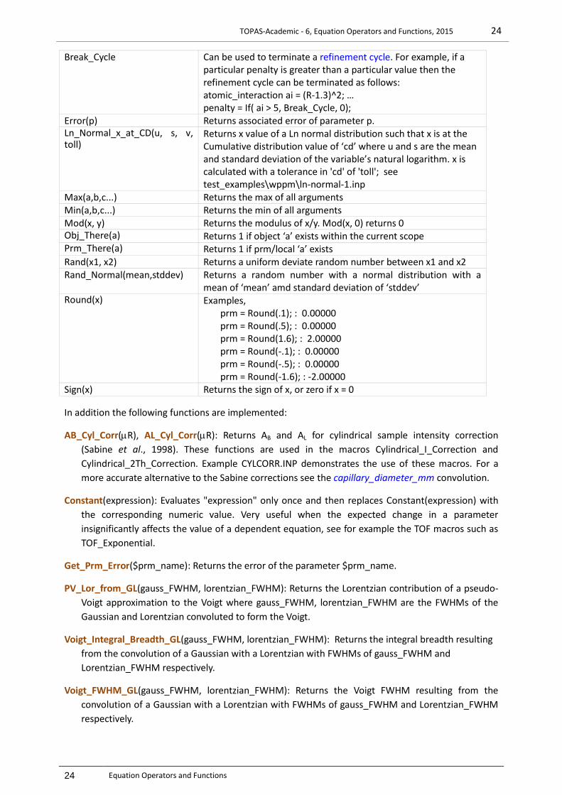
Break Can be used to terminate loops implied by the equations atomic_interaction, box_interaction and grs_interaction.
TOPAS-Academic - 6, Equation Operators and Functions, 2015 24
24 Equation Operators and Functions
Break_Cycle Can be used to terminate a refinement cycle. For example, if a particular penalty is greater than a particular value then the refinement cycle can be terminated as follows: atomic_interaction ai = (R-1.3)^2; … penalty = If( ai > 5, Break_Cycle, 0);
Error(p) Returns associated error of parameter p. Ln_Normal_x_at_CD(u, s, v, toll)
Returns x value of a Ln normal distribution such that x is at the Cumulative distribution value of ‘cd’ where u and s are the mean and standard deviation of the variable’s natural logarithm. x is calculated with a tolerance in 'cd' of 'toll'; see test_examples\wppm\ln-normal-1.inp
Max(a,b,c...) Returns the max of all arguments
Min(a,b,c...) Returns the min of all arguments
Mod(x, y) Returns the modulus of x/y. Mod(x, 0) returns 0
Obj_There(a) Returns 1 if object ‘a’ exists within the current scope
Prm_There(a) Returns 1 if prm/local ‘a’ exists
Rand(x1, x2) Returns a uniform deviate random number between x1 and x2
Rand_Normal(mean,stddev) Returns a random number with a normal distribution with a mean of ‘mean’ amd standard deviation of ‘stddev’
Round(x) Examples, prm = Round(.1); : 0.00000 prm = Round(.5); : 0.00000 prm = Round(1.6); : 2.00000 prm = Round(-.1); : 0.00000 prm = Round(-.5); : 0.00000 prm = Round(-1.6); : -2.00000
Sign(x) Returns the sign of x, or zero if x = 0
In addition the following functions are implemented:
AB_Cyl_Corr(R), AL_Cyl_Corr(R): Returns AB and AL for cylindrical sample intensity correction
(Sabine et al., 1998). These functions are used in the macros Cylindrical_I_Correction and
Cylindrical_2Th_Correction. Example CYLCORR.INP demonstrates the use of these macros. For a
more accurate alternative to the Sabine corrections see the capillary_diameter_mm convolution.
Constant(expression): Evaluates "expression" only once and then replaces Constant(expression) with
the corresponding numeric value. Very useful when the expected change in a parameter
insignificantly affects the value of a dependent equation, see for example the TOF macros such as
TOF_Exponential.
Get_Prm_Error($prm_name): Returns the error of the parameter $prm_name.
PV_Lor_from_GL(gauss_FWHM, lorentzian_FWHM): Returns the Lorentzian contribution of a pseudo-
Voigt approximation to the Voigt where gauss_FWHM, lorentzian_FWHM are the FWHMs of the
Gaussian and Lorentzian convoluted to form the Voigt.
Voigt_Integral_Breadth_GL(gauss_FWHM, lorentzian_FWHM): Returns the integral breadth resulting
from the convolution of a Gaussian with a Lorentzian with FWHMs of gauss_FWHM and
Lorentzian_FWHM respectively.
Voigt_FWHM_GL(gauss_FWHM, lorentzian_FWHM): Returns the Voigt FWHM resulting from the
convolution of a Gaussian with a Lorentzian with FWHMs of gauss_FWHM and Lorentzian_FWHM
respectively.

TOPAS-Academic - 6, Equation Operators and Functions, 2015 25
25 Equation Operators and Functions
Yobs_dx_at(#x): Returns the step size in the observed data at the x-axis position #x; can be used in all
sub xdd dependent equations. If the step size in the x-axis is equidistant then Yobs_dx_at is
converted to a constant corresponding to the step size in the data.
Sites_Geometry_Distance($Name) Sites_Geometry_Angle($Name) Sites_Geometry_Dihedral_Angle($Name)
3.1 ... 'If' and nested 'if' statements
'Sum' and 'If' statements can be used in parameter equations, for example:
str...
prm a .1
prm b .1
lor_fwhm = If(Mod(H, 2)==0, a Tan(Th), b Tan(Th));
Min and Max can also be used in parameter equations; for example the following is valid:
prm a .1
th2_offset = Min(Max(a, -.2), .2);
'If' should be preferred in non-attribute equations as analytical derivatives are possible; they can be
nested, for example:
prm cs 200 update =
If(Val < 10, 10,
If(Val > 10000, 10000,
Val
)
);
For those who are familiar with if/else statements then the IF THEN ELSE ENDIF macros as defined in
TOPAS.INC can be used as follows:
IF a > b THEN
a ‘ return expression value
ELSE
b ‘ return expression value
ENDIF
3.2 ... Floating point exceptions
An exception is thrown when an invalid floating point operation is encountered, examples are:
Divide by zero.
Sqrt(x) for x < 0
Ln(x) for x <= 0
ArcCos(x) for x -1 or x 1
Exp(x) produces an overflow for x ~ 700
(-x)^y for x 0 and y not an integer
Tan(x) evaluates to Infinity for x = n Pi/2, Abs(n) = 1, 3, 5,...
min/max equations, or Min/Max functions or ‘If’ statements can be used to avoid invalid floating point
operations. Equations can also be manipulated to yield valid floating point operations, for example,
Exp(-1000) can be used in place of 1/Exp(1000).
TOPAS-Academic - 6, The Minimization Routines, 2015 26
26 The Minimization Routines
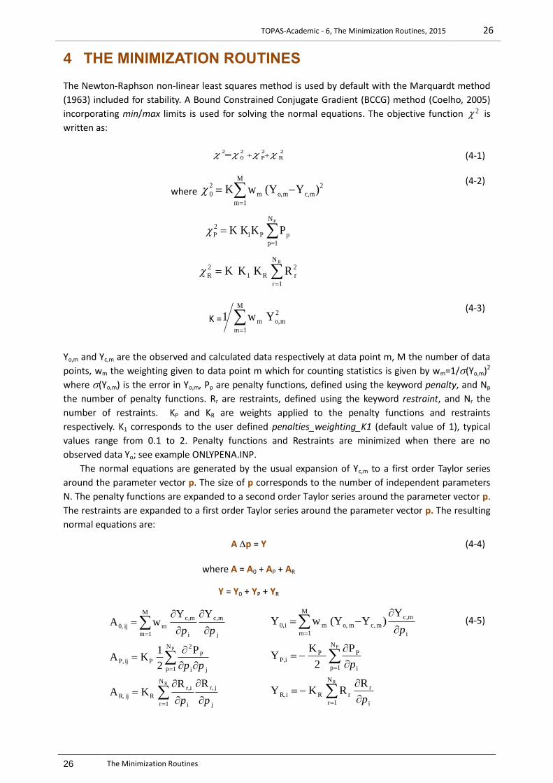
4 THE MINIMIZATION ROUTINES
The Newton-Raphson non-linear least squares method is used by default with the Marquardt method
(1963) included for stability. A Bound Constrained Conjugate Gradient (BCCG) method (Coelho, 2005)
incorporating min/max limits is used for solving the normal equations. The objective function 2 is
written as:
2
R
2
P
2
0
2 (4-1)
where
M
1m
2
mc,mo,m
2
0 )Y(Y wK
PN
1p
pP1
2
P P K K K
RN
1r
2
rR1
2
R R K K K
(4-2)
K =
M
1m
2
mo,m Yw1 (4-3)
Yo,m and Yc,m are the observed and calculated data respectively at data point m, M the number of data
points, wm the weighting given to data point m which for counting statistics is given by wm=1/(Yo,m)2
where (Yo,m) is the error in Yo,m, Pp are penalty functions, defined using the keyword penalty, and Np
the number of penalty functions. Rr are restraints, defined using the keyword restraint, and Nr the
number of restraints. KP and KR are weights applied to the penalty functions and restraints
respectively. K1 corresponds to the user defined penalties_weighting_K1 (default value of 1), typical
values range from 0.1 to 2. Penalty functions and Restraints are minimized when there are no
observed data Yo; see example ONLYPENA.INP.
The normal equations are generated by the usual expansion of Yc,m to a first order Taylor series
around the parameter vector p. The size of p corresponds to the number of independent parameters
N. The penalty functions are expanded to a second order Taylor series around the parameter vector p.
The restraints are expanded to a first order Taylor series around the parameter vector p. The resulting
normal equations are:
A p = Y (4-4)
where A = A0 + AP + AR
Y = Y0 + YP + YR
R
P
N
1r j
jr,
i
ir,
Rij R,
N
1p ji
P
2
Pij P,
M
1m j
mc,
i
mc,
mij 0,
RR K A
P
2
1 K A
YY w A
pp
pp
pp
R
R K Y
P
2
K Y
Y)Y(Y w Y
R
P
N
1r i
rrRiR,
N
1p i
PPiP,
M
1m i
mc,
m c,m o,mi0,
p
p
p
(4-5)
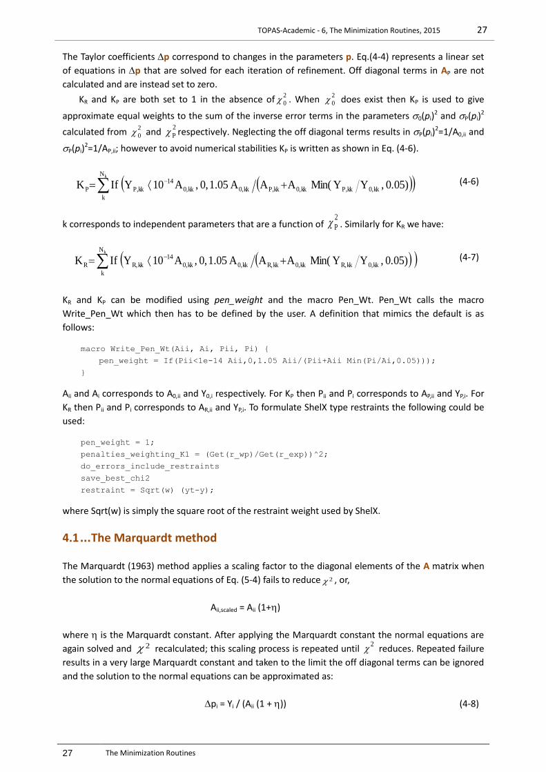
TOPAS-Academic - 6, The Minimization Routines, 2015 27
27 The Minimization Routines
The Taylor coefficients p correspond to changes in the parameters p. Eq.(4-4) represents a linear set
of equations in p that are solved for each iteration of refinement. Off diagonal terms in AP are not
calculated and are instead set to zero.
KR and KP are both set to 1 in the absence of2
0 . When 2
0 does exist then KP is used to give
approximate equal weights to the sum of the inverse error terms in the parameters 0(pi)2 and P(pi)
2
calculated from 2
0 and 2
P respectively. Neglecting the off diagonal terms results in P(pi)2=1/A0,ii and
P(pi)2=1/AP,ii; however to avoid numerical stabilities KP is written as shown in Eq. (4-6).
kN
k
kk0,kkP,kk0,kkP,kk0,kk0,
14
kkP,P )0.05 ,YYMin( AAA 05.1 0, ,A10 Y If K (4-6)
k corresponds to independent parameters that are a function of 2
P . Similarly for KR we have:
kN
k
kk0,kkR,kk0,kkR,kk0,kk0,
14
kkR,R )0.05 ,YYMin( AAA 05.1 0, ,A10 Y If K (4-7)
KR and KP can be modified using pen_weight and the macro Pen_Wt. Pen_Wt calls the macro
Write_Pen_Wt which then has to be defined by the user. A definition that mimics the default is as
follows:
macro Write_Pen_Wt(Aii, Ai, Pii, Pi) {
pen_weight = If(Pii<1e-14 Aii,0,1.05 Aii/(Pii+Aii Min(Pi/Ai,0.05)));
}
Aii and Ai corresponds to A0,ii and Y0,i respectively. For KP then Pii and Pi corresponds to AP,ii and YP,i. For
KR then Pii and Pi corresponds to AR,ii and YP,i. To formulate ShelX type restraints the following could be
used:
pen_weight = 1;
penalties_weighting_K1 = (Get(r_wp)/Get(r_exp))^2;
do_errors_include_restraints
save_best_chi2
restraint = Sqrt(w) (yt-y);
where Sqrt(w) is simply the square root of the restraint weight used by ShelX.
4.1 ... The Marquardt method
The Marquardt (1963) method applies a scaling factor to the diagonal elements of the A matrix when
the solution to the normal equations of Eq. (5-4) fails to reduce 2 , or,
Aii,scaled = Aii (1+)
where is the Marquardt constant. After applying the Marquardt constant the normal equations are
again solved and 2 recalculated; this scaling process is repeated until 2
reduces. Repeated failure
results in a very large Marquardt constant and taken to the limit the off diagonal terms can be ignored
and the solution to the normal equations can be approximated as:
pi = Yi / (Aii (1 + )) (4-8)

TOPAS-Academic - 6, The Minimization Routines, 2015 28
28 The Minimization Routines
The Marquardt method is used when the refinement comprises observed data Yo. The keyword
no_normal_equations prevents the use of the Marquardt method.
The Marquardt constant is automatically determined each iteration. Its determination is based
on the actual change in 2 and the expected change in 2 .
4.2 ... Approximating the A matrix - the BFGS method
The approximate_A keyword can be used to approximate the A matrix, Eq. (4-4), without the need to
calculate the A matrix dot products. The approximation is based on the BFGS method (Broyden, 1970;
Fletcher, 1970; Goldfarb, 1970; Shanno, 1970). BCCG is used by default for solving the normal
equations, alternatively, LU-decomposition can be used if use_LU is defined and the A matrix is not
sparse. Note, that LU-decomposition requires the full A matrix and thus it may be too memory
intensive for problems with 10s of thousands of parameters. LU-decomposition can also be too slow
when the number of parameters is greater than about one thousand parameters.
Approximating A is useful when the calculation of the A matrix dot products is proving too
expensive. When penalties dominates a refinement then the use of approximate_A may also improve
convergence. approximate_A cannot be used with line_min or use_extrapolation.
The single crystal refinement examples AE14-APPROX-A.INP and AE1-APPROX-A.INP are cases
where the use of approximate_A achieves convergence is less time than with the calculated A matrix.
When using approximate_A the A matrix can be made sparse by defining
A_matrix_memory_allowed_in_Mbytes and/or A_matrix_elements_tollerance. This allows for
refinements with a large number of independent parameters.
4.3 ... Line minimization and Parameter extrapolation
Line minimization better known as the steepest decent method is invoked with the keyword line_min.
It uses a direction in parameter space given by pi=Yi/Aii to minimize on 2 (p+p) by adjusting .
Parameter Extrapolation, invoked with the keyword use_extrapolation, uses parabolic
extrapolation of the parameters as a function of iteration, or, is adjusted such that 2 (a2+b+c) is
minimized where for a particular parameter pi at iteration k we have ai=(y12y2+y3)/2, bi=(y3y1)/2 and
ci=y2 where y1=(pi,k-5+pi,k-4)/2, y2=(pi,k-3+pi,k-2)/2 and y3 = (pi,k-1+pi,k-0)/2. Parameter Extrapolation
encompasses the last six sets of parameter values. In cases where both 2
0 and 2
P exists then
Parameter Extrapolation reduces possible oscillatory behaviour in2
P . Parameter extrapolation when
used with Line Minimization can increase the rate of convergence when refining on penalties only.
Line minimization and Parameter Extrapolation have relatively small memory foot prints and thus
can be useful when the A matrix consumes too much memory. Alternatively the approximate_A
keyword can be used.
Line minimization with the full A matrix calculation (no approximate_A defined) can increase the
rate of convergence on problems like Pawley refinement.
4.4 ... The Conjugate Gradient Solution method
The bound constrained conjugate gradient method (Coelho, 2005) used for solving the normal
equations greatly assists in convergence of the non-linear least squares process. min/max limits are
dynamically recalculated during the solution process for min/max limits that are a function of
independent parameters. For example, to constrain site occupancies on three sites to full occupancy
with three atomic species each with occupancy of 1 the following could be defined (see
test_examples\occ-constrain.inp):

TOPAS-Academic - 6, The Minimization Routines, 2015 29
29 The Minimization Routines
site Ni x .11 y .22 z .33
occ Ni ni1 0.20000 min 0 max 1
occ Zr zr1 0.30000 min 0 max = 1 - ni1;
occ Ca ca1 = 1 - ni1 - zr1; : 0.50000
site Zr x .21 y .32 z .43
occ Ni ni2 0.40000 min 0 max = 1 - ni1;
occ Zr zr2 0.50000 min 0 max = 1 - ni2;
occ Ca ca2 = 1 - ni2 - zr2; : 0.10000
site Ca x .31 y .42 z .53
occ Ni ni3 = 1 - ni1 - ni2; : 0.40000
occ Zr zr3 = 1 - zr1 - zr2; : 0.20000
occ Ca ca3 = 1 - ca1 - ca2; : 0.40000
' Occupancy on sites add up to 1
prm = ni1 + zr1 + ca1; : 1.00000
prm = ni2 + zr2 + ca2; : 1.00000
prm = ni3 + zr3 + ca3; : 1.00000
' Individual species add up to 1
prm = ni1 + ni2 + ni3; : 1.00000
prm = zr1 + zr2 + zr3; : 1.00000
prm = ca1 + ca2 + ca3; : 1.00000
4.5 ... Restraints and Penalties
A restraint can be reformulated using a penalty by squaring the restraint, for example:
restraint = a (x - b);
is equivalent to
penalty = a^2 (x - b)^2;
In the case of the restraint the off-diagonal terms AR,ij are calculated when approximate_A (the BFGS
method) is not defined. In the case of the penalty the off-diagonal terms AP,ij is set to zero. Restraints
often converge faster than equivalent penalties due to the use of the off-diagonal terms (compare
ROSENBROCK-10.INP with ROSENBROCK-10-RESTRAINT.INP). Penalties are useful for functions that
are not to be squared; these include negative functions such as the GRS series atomic interaction (see
ALVO4-GRS-AUTO.INP).
For efficiency the AR matrix is treated as a sparse matrix which is combined with A0 (if it exists)
where A0 could be either sparse or dense. When approximate_A is used then the diagonal elements of
A0, AP, and AR are not calculated; instead they are approximated by the BFGS method.
When approximate_A is used and both penalties and restraints are defined then this effectively
means that the restraints are treated as penalties. The following for example:
Case 1
approximate_A
prm p1 1 prm r1 1
penalty !P1 = 5^2 (p1 - 7)^2;
penalty !P2 = 6^2 (p1 - 8)^2;
restraint !R1 = 7 (r1 - 9);
restraint !R2 = 8 (r1 - 10);
will have similar but not identical convergence to the following:
Case 2
prm p1 1 prm r1 1

TOPAS-Academic - 6, The Minimization Routines, 2015 30
30 The Minimization Routines
penalty !P1 = 5^2 (p1 - 7)^2;
penalty !P2 = 6^2 (p1 - 8)^2;
penalty !P3 = 7^2 (r1 - 9)^2;
penalty !P4 = 8^2 (r1 - 10)^2;
In Case 1 the diagonal elements of the A matrices are:
AP,p1p1 = (½) 2(P1+P2) / p12
AR,r1r1 = ( R1/ r1)2 + ( R2/ r1)2
In Case 2 they are:
AP,p1p1 = (½) 2(P1+P2) / p12
AP,r1r1 = (½) 2(R12+R22) / r12
The difference in behavior between penalties and restraints can be seen by comparing ROSENBROCK-
10.INP to ROSENBROCK-10-RESTRAINT.INP. In 500,000 iterations we have:
ROSENBROCK-10.INP: 71 iterations on average to convergence
ROSENBROCK-10-RESTRAINT.INP: 47 iterations on average to convergence
The restraints converge faster as the AR,ij elements are calculated. Approximating AR,ij by defining
approximate_A in ROSENBROCK-10-RESTRAINT.INP gives the fastest convergence time wise:
ROSENBROCK-10-RESTRAINT.INP: 71 iterations on average to convergence
Many penalties however cannot be formulated as a restraint, RASTRIGIN.INP for example, and in these
cases penalties are mandatory.
4.6 ... Minimizing on penalties only
When there are no observed data or when only_penalties is defined then by default the BFGS method
is used, see examples ROSENBROCK-10.INP and HOCK.INP. For ‘penalties only’ the BFGS method
typically converges faster than line_min/use_extrapolation; this however for ‘penalties only’ it can be
overridden with the use of line_min.
4.7 ... Saved refined values and save_best_chi2
Values saved on termination of refinement are determined as follows:
If continue_after_convergence is NOT defined and save_best_chi2 is NOT defined then values
saved corresponds to those of the last iteration.
If continue_after_convergence is NOT defined and save_best_chi2 is defined then values saved
corresponds to those that gave the best Chi2.
If continue_after_convergence is defined and save_best_chi2 is NOT defined then values saved
corresponds to those that gave the best Rwp.
If continue_after_convergence is defined and save_best_chi2 is defined then values saved
corresponds to those that gave the best Chi2
When there are no penalties or restraints then the best Chi2 corresponds to the best Rwp.

TOPAS-Academic - 6, The Minimization Routines, 2015 31
31 The Minimization Routines
4.8 ... Error calculation
Errors are calculated for all independent and non-independent parameters that are single valued
when any of the following is defined:
do_errors : Errors calculated without the inclusion of penalties and restraints in the A matrix.
do_errors_include_penalties : Errors calculated with the inclusion of penalties in the A matrix.
do_errors_include_restraints : Errors calculated with the inclusion of restraints in the A matrix.
4.9 ... Error determination using SVD
Errors have previously been determined from a covariance matrix obtained by LU decomposition. Version 6 uses
Singular Value Decomposition (SVD) with resulting errors typically smaller for strongly correlated parameters.
Additionally SVD errors more closely resemble those obtained by the boot strap method. bootstrap_errors are
potentially more accurate as it considers parameter limits; for example the fact that intensities are positive is not
considered by matrix inversion.
The keyword use_LU_for_errors can be used to force the use of LU decomposition. The three means of
determining errors are demonstrated in a Pawley refinement of Y2O23 in the following INP files:
Test_examples\svd-errors\y2o3a-lu.inp
Test_examples\svd-errors\y2o3a-svd.inp
Test_examples\svd-errors\y2o3a-boot.inp
Comparisons showing the similarity between the bootstrap and SVD errors are seen in the following INP
snippets:
LU Full_Axial_Model(12, 15, 12, 5.1, @ 8.56191`_0.06668)
SVD Full_Axial_Model(12, 15, 12, 5.1, @ 8.56190`_0.05045)
Boot Full_Axial_Model(12, 15, 12, 5.1, @ 8.56191`_0.04988)
LU ZE(@, 0.08739`_0.00037)
SVD ZE(@, 0.08739`_0.00018)
Boot ZE(@, 0.08739`_0.00020)
LU Cubic(@ 10.605643`_0.000013)
SVD Cubic(@ 10.605643`_0.000019)
Boot Cubic(@ 10.605643`_0.000020)
LU CS_L(csl, 369.29260`_10.37269)
SVD CS_L(csl, 369.29260`_3.13254)
Boot CS_L(csl, 369.27962`_2.92401)
LU bkg @ 199.402275`_21.4050278 -8.89848018`_1.85486669 47.9112026`_1.841 83168..
SVD bkg @ 199.407893`_1.12005938 -8.91085058`_1.84031795 47.9154076`_1.69533286...
Boot bkg @ 199.402275`_0.92177244 -8.89848018`_1.47936429 47.9112026`_1.20647356...
LU SVD Boot
0 0 2 ... 1.02580`_0.12061 1.02578`_0.06440 1.02580`_0.04088
2 1 1 ... 65.81458`_0.43091 65.81449`_0.43023 65.81458`_0.33495
0 2 2 ... 0.00000`_0.07691 0.00003`_0.07645 0.00000`_0.00138
2 2 2 ... 1197.20758`_2.76303 1197.20695`_2.5964 1197.20758`_3.88388
3 2 1 ... 2.55249`_32911418.00252 2.55243`_0.12020 2.55249`_0.07342
2 3 1 ... 2.55249`_14161941.24442 2.55243`_0.12020 2.55249`_0.07342
0 0 4 ... 374.70367`_1.83981 374.70343`_1.71262 374.70367`_1.46988
4 1 1 ... 88.85977`_0.91217 88.85964`_0.91858 88.85977`_0.65040
4 0 2 ... 10.65522`_16487463.58725 10.65514`_0.26162 10.65522`_0.19312
0 4 2 ... 10.65522`_16487463.58725 10.65514`_0.26162 10.65522`_0.19312
3 3 2 ... 141.18328`_1.24215 141.18308`_1.28901 141.18328`_1.07037
4 2 2 ... 21.67021`_0.61141 21.67012`_0.59628 21.67021`_0.42625
3 4 1 ... 119.04993`_124057100727963620 119.04970`_0.91382 119.04993`_0.88560
4 3 1 ... 119.04993`_124057100727963630 119.04970`_0.91382 119.04993`_0.88560
5 2 1 ... 44.77524`_31163203794483688 44.77511`_0.63035 44.77524`_0.43513
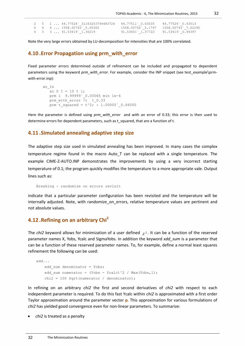
TOPAS-Academic - 6, The Minimization Routines, 2015 32
32 The Minimization Routines
2 5 1 ... 44.77524`_31163203794483724 44.77511`_0.63035 44.77524`_0.43513
0 4 4 ... 1558.50793`_5.05350 1558.50756`_5.1797 1558.50793`_7.02290
4 3 3 ... 91.53419`_1.30219 91.53401`_1.37722 91.53419`_0.94397
Note the very large errors obtained by LU-decomposition for intensities that are 100% correlated.
4.10 . Error Propagation using prm_with_error
Fixed parameter errors determined outside of refinement can be included and propagated to dependent
parameters using the keyword prm_with_error. For example, consider the INP snippet (see test_example\prm-
with-error.inp):
xo_Is
xo 0 I = 10 t i;
prm i 9.99999`_0.00065 min 1e-6
prm_with_error !t 1_0.33
prm t_squared = t^2; : 1.00000`_0.66000
Here the parameter is defined using prm_with_error and with an error of 0.33; this error is then used to
determine errors for dependent parameters, such as t_squared, that are a function of t.
4.11 . Simulated annealing adaptive step size
The adaptive step size used in simulated annealing has been improved. In many cases the complex
temperature regime found in the macro Auto_T can be replaced with a single temperature. The
example CIME-Z-AUTO.INP demonstrates the improvements by using a very incorrect starting
temperature of 0.1; the program quickly modifies the temperature to a more appropriate vale. Output
lines such as:
Breaking - randomize on errors revisit
indicate that a particular parameter configuration has been revisited and the temperature will be
internally adjusted. Note, with randomize_on_errors, relative temperature values are pertinent and
not absolute values.
4.12 . Refining on an arbitrary Chi2
The chi2 keyword allows for minimization of a user defined 2 . It can be a function of the reserved
parameter names X, Yobs, Ycalc and SigmaYobs. In addition the keyword xdd_sum is a parameter that
can be a function of these reserved parameter names. To, for example, define a normal least squares
refinement the following can be used:
xdd...
xdd_sum denominator = Yobs;
xdd_sum numerator = (Yobs - Ycalc)^2 / Max(Yobs,1);
chi2 = 100 Sqrt(numerator / denominator);
In refining on an arbitrary chi2 the first and second derivatives of chi2 with respect to each
independent parameter is required. To do this fast Ycalc within chi2 is approximated with a first order
Taylor approximation around the parameter vector p. This approximation for various formulations of
chi2 has yielded good convergence even for non-linear parameters. To summarize:
chi2 is treated as a penalty

TOPAS-Academic - 6, The Minimization Routines, 2015 33
33 The Minimization Routines
For each independent parameter, a definite minima in chi2 is bracketed and inverse parabolic
interpolation used to determine the minima of chi2 with respect to that parameter. In the
calculation of chi2, Ycalc is replaced with its first order Taylor approximation and thus the full Ycalc
is only calculated once per refinement iteration and not 100s of times.
Finding the minima and the curvature of chi2 with respect to each parameter yields 1st and 2nd
order derivatives of chi2 with respect to each parameter.
The BFGS method (approximate_A) is then used to solve the resulting linear equations with off
diagonal terms approximated according to the BFGS method.
The BCCG method incorporating the Marquardt method with automatic Marquardt constant
determination is used to solve the matrix equations.
The Rietveld refinement test_example\chi2-ceo2.inp example demonstrates various scenarios.
Case 1) Here’s output when NOT using chi2.
0 Time 0.05 Rwp 26.630 0.000 MC 0.00 0
1 Time 0.06 Rwp 16.651 -9.979 MC 0.06 1
2 Time 0.06 Rwp 7.510 -9.141 MC 0.02 1
3 Time 0.08 Rwp 6.955 -0.556 MC 0.01 1
4 Time 0.08 Rwp 6.943 -0.011 MC 0.00 1
5 Time 0.08 Rwp 6.923 -0.020 MC 0.00 1
6 Time 0.09 Rwp 6.923 -0.000 MC 0.18 1
--- 0.094 seconds ---
Case 2) Here’s output when NOT using chi2 but using approximate_A.
0 Time 0.05 Rwp 26.630 0.000 MC 0.00 0
1 Time 0.06 Rwp 16.883 -9.747 MC 0.00 0
...
16 Time 0.13 Rwp 6.950 -0.002 MC 0.04 1
17 Time 0.14 Rwp 6.949 -0.002 MC 0.09 1
18 Time 0.14 Rwp 6.949 -0.000 MC 0.29 1
--- 0.14 seconds ---
Case 3) Here’s output using chi2 defined for normal least squares
0 Time 0.03 Rwp 26.630 0.000 MC 0.00 0 P 26.63020
1 Time 0.06 Rwp 15.897 -10.733 MC 0.00 0 P 15.89696
...
13 Time 0.33 Rwp 6.974 -0.021 MC 0.00 1 P 6.97366
14 Time 0.34 Rwp 6.958 -0.016 MC 0.00 1 P 6.95755
15 Time 0.38 Rwp 6.951 -0.006 MC 0.00 1 P 6.95122
The chi2 case (3) looks similar to case (2); however the path towards the minima is different as the
chi2 procedure is very different to normal least squares refinement.
4.13 . Informing on unrefined parameters
Parameters that do not take part in a refinement are now reported, for example, the following:
prm a 1
prm b 1
where a and b are not used in any equations that are part of refinement will result in the following
output:
Number of independent parameters not taking part in refinement: 2
prm_10: a
prm_10: b
TOPAS-Academic - 6, The Minimization Routines, 2015 34
34 The Minimization Routines
The val_on_continue attribute of unrefined parameters are executed at the end of convergence. It can
be useful, for example,
prm a 1 val_on_continue = b = 2; ‘ this sets the parameter b to 2.
4.14 . Summary, Iteration and Refinement Cycle
Table 4-1 shows various keyword usages for typical refinement problems. The term “refinement cycle”
is used to describe a single convergence. The reserved parameter Cycle returns the current refinement
cycle with counting starting at zero. The reserved parameter Cycle_Iter returns the current iteration
within a Cycle with counting starting at zero.
Table 4-1 Keyword sequences for various refinement types
Refinement type Keywords to use Comments
Rietveld refinement
No penalties
Marquardt refinement.
A matrix calculation.
Rietveld refinement with
a moderate number of penalties.
line_min (Maybe) Line minimization used if line_min.
Marquardt refinement.
A matrix calculation.
Rietveld refinement dominated by penalties
approximate_A BFGS method of refinement.
A matrix approximation.
Pawley refinement line_min Line minimization.
Marquardt refinement.
A matrix calculation.
Penalties only BFGS method of refinement.
A matrix approximation.
Refinements with a large number of parameters
approximate_A BFGS method of refinement.
A matrix approximation.
4.15 . quick_refine and computational issues
The computationally dominant factor of calculating Eq. (4-5) is problem dependent. For Rietveld
refinement with a moderate number of parameters then the calculation of the peak parameter
derivatives may well be the most expensive. On the other hand for Rietveld refinement with a large
number of structural parameters and data points then the calculation of the A1,ij dot products would
be the dominant factor, where, the number of operations scale by M(N2+N)/2. Before the development
of the BCCG routine (Coelho, 2005), the solution to the normal equations, Eq. (4-4)), was also very
expensive.
For structure solution from powder data by simulated annealing, the keyword
yobs_to_xo_posn_yobs can be used to reduce the number of data points M; thus reducing the number
of operations in the A1,ij dot products, see the Decompose macro in example CIME-DECOMPOSE.INP.
The quick_refine keyword removes parameters during a refinement cycle thus shrinking the size of
the A matrix by reducing N. Parameters are removed if the condition defined in Eq. (4-9) is met for
three consecutive iterations.
Y NK nequick_refi 0.01 p ii (4-9)

TOPAS-Academic - 6, The Minimization Routines, 2015 35
35 The Minimization Routines
Alternatively, parameters can be removed or reinstated during a refinement cycle using
quick_refine_remove. This keyword provides a means of performing block refining. If
quick_refine_remove is not defined then all parameters are reinstated at the start of refinement cycles.
4.16 . Auto_T and randomize_on_errors
It is sometimes difficult to formulate optimum val_on_continue functions for simulated annealing. This
is especially true in structure solution using rigid bodies where optimum randomization of the rigid
body parameters can be difficult to ascertain. randomize_on_errors is a means of automatically
randomizing parameters based on the approximate errors in the parameters as given in Eq. (4-10),
where T is the current temperature and K is as defined in Eq. (4-3).
AK T 0.02 ,1))1 Sign(Rand( Q p iii (4-10)
Q is a scaling factor determined such that convergence to a previous parameter configuration occurs
7.5% of the time on average. When randomize_on_errors is used the magnitude of the temperature(s)
is not of significance but the relative variation in temperature(s) are.
The macro Auto_T includes quick_refine, randomize_on_errors and a temperature regime. It has
shown to be adequate for a wide range of simulated annealing examples, see example CIME-Z-
AUTO.INP. Note, when val_on_continue is defined then the corresponding parameter is not
randomized according to randomize_on_errors.

TOPAS-Academic - 6, The Minimization Routines, 2015 36
36 The Minimization Routines
4.17 . Criteria of fit
Table 4-2: Criteria of fit (see Young 1993 for details). Yo,m and Yc,m are the observed and calculated data
respectively at data point m, Bkgm the background at data point m, M the number of data points, P the
number of parameters, wm the weighting given to data point m which for counting statistics is given by
wm=1/(Yo,m)2 where (Yo,m) is the error in Yo,m, and I"o",k and Ic,k the "observed" and calculated
intensities of the kth reflection.
Criteria of fit Definition
“R-pattern", Rp'
(background corrected)
mo
mcmo
pY
YYR
,
,,
mmo
mcmo
pBkgY
YYR
,
,,'
"R-weighted pattern",
Rwp
Rwp'(background
corrected)
2
,
2
,,
mom
mcmom
wp
Yw
YYwR
2
,
2
,,'
mmom
mcmom
wpBkgYw
YYwR
"R-expected", Rexp
(background corrected)
2
,
exp
momYw
PMR
2
,
exp 'mmom BkgYw
PMR
"Goodness of fit", GOF
PM
YYw
R
RchiGOF
mcmomwp
2
,,
exp
"R-Bragg", RB
ko
kcko
BI
IIR
,""
,,""
"Durbin-Watson ", d,
1971;
Hill & Flack, 1987
mcmomM
m
m
M
m
mm
YYY
Y
YY
d ,,
1
2
2
2
1
;

TOPAS-Academic - 6, Peak Generation and "peak_type", 2015 37
37 Peak Generation and "peak_type"
5 PEAK GENERATION AND "PEAK_TYPE"
Convolution implies integration; a function analytically integrated is exact whereas numerical
integration is an approximation with an accuracy dependent on the step size used for integration.
Accurate numerical convolution is used when analytical convolution is not possible; this makes it
possible to include complex functions in the generation of peak shapes. Numerical convolution is
important in regards to laboratory powder diffraction data as many of the instrument aberration
functions cannot be convoluted analytically. The process of convolution from a fundamental
parameters perspective is an approximation whereby second order effects and higher are typically
neglected. These approximations are valid except for extreme cases that are unlikely to exist in
practice, for example, axial divergence with Soller slits acceptance angles that are greater than about
12 degrees.
5.1 ... Source emission profiles
Generation of the emission profile is the first step in peak generation. It comprises EM lines, EMk, each
of which is a Voigt comprising the parameters la, lo, lh and lg. The reserved parameter name Lam is
assigned the lo value of the EMk line with the largest la value, this EMk will be called EMREF. It is used
to calculate d-spacings. The interpretation of EM data is dependent on peak_type. For all peak types
the position 2k calculated for a particular emission line for a particular Bragg position of 2 is
determined as follows:
360
2
,2
d
lokEMArcSink where SinloEMREFd 2
2 for xo_Is phases corresponds to the xo parameter. 2 for d_Is phases is given by the Bragg equation
2=ArcSin(Lam/(2 d)) 360/Pi where d corresponds to the value of the d parameter. 2 values for str
and hkl_Is phases are calculated from the lattice parameters.
The FWHWk in °2 for an EMk line is determined from the relations provided in Table 5-1.
When the keyword no_th_dependence is defined then the calculation of 2k is determined from
2k = 2 + EM(lo, i)
The macro No_Th_Dependence can be used when refining on non-X-ray data or fitting to negative 2
values (see example NEGX.INP).
The x-axis extent (x1, x2) to which an EM line is calculated is determined by:
axymin_on_ym
0)"x of EMREF("Intensity
"x2x1xi,EMof"Intensity
where EMREF corresponds to the emission profile with the largest la value. The default for
ymin_on_ymax is 0.001. Emission profile data have been taken from Hölzer et al. (1997) and are stored
in *.LAM files in the LAM directory.

TOPAS-Academic - 6, Peak Generation and "peak_type", 2015 38
38 Peak Generation and "peak_type"
Table 5-1 FWHWk in °2 for an EMk line for the different peak types.
FP peak type
360, Tan
LAM
lhkEMFWHM k
PV peak type )(
,_
lhEMREF
lhkEMfwhmpvFWHMk
SPVII peak type )(
,12
lhEMREF
lhkEMhFWHM k ,
)(
,22
lhEMREF
lhkEMhFWHM k
SPV peak type )(
,1_2
lhEMREF
lhkEMhspvFWHM k ,
)(
,2_2
lhEMREF
lhkEMhspvFWHM k
5.2 ... Peak generation and peak types
Phase peaks P are generated as follows:
P = Get(scale) Get(all_scale_pks) EM(peak_type) Convolutions (5-1)
where the emission profile (EM) is first generated with emission profile lines of type peak_type; the
symbol denotes convolution. Peaks are then convoluted with any defined convolutions, multiplied
by the scale parameter, multiplied by any defined scale_pks, and then multiplied by an intensity
parameter. In the process peaks shapes can mostly be described in a fundamental parameters
approach (Cheary et al., 2004). For xo_Is, d_Is and hkl_Is phases the intensity is given by the I
parameter. For str phases it corresponds to the square of the structure factor F2(hkl). Convolutions are
normalized and do not change the area under a peak except for the capillary_diameter_mm and
lpsd_th2_angular_range_degrees convolutions. The area under the emission profile is determined by
the sum of the la parameters; typically they add up to 1.
The definitions of the pseudo-Voigt and PearsonVII functions are provided in Table 5-2 (symmetric
functions) and Table 5-3 (split functions). The following terms are used:
Symmetric functions
x (2-2k) where 2k is the position of the kth reflection
fwhm full width at half maximum
PV mixing parameter
Asymmetric functions
fwhm1, fwhm2 fwhm for the left and right composite function
m1, m2 Exponents for the composite functions
PV mixing parameters for the composite functions

TOPAS-Academic - 6, Peak Generation and "peak_type", 2015 39
39 Peak Generation and "peak_type"
Table 5-2 Unit area peak types for symmetric functions.
Profile Function Definition
Gaussian, GUA(x)
2
2
21
fwhm
xgExp
fwhm
gxGUA
where 221 Lng , 242 Lng
Lorentzian, LUA(x)
2
2
21 1fwhm
xl
fwhm
lxLUA
where 21 l , 42 l
PseudoVoigt, PVUA(x) xGxLPV UAUA 1
Table 5-3 Unit area peak types for split functions.
Profile Function Definition
Split PearsonVII, SPVII PVII_RightPVII_LeftSPVII
where
axbm12
11PVII_Left
0for x
axbm22
21PVII_Right
x0for
2
21
1
21
21
21
2
2
1
1
bm
m
bm
ma
21/1
1 112 hb m , 22/1
2 212 hb m
121 hfwhm , 222 hfwhm , 21 hhfwhm
Split PseudoVoigt, SPV aa 1PV_RightPV_Left2SPV
where
1,1PVPV_Left h 0for x
2,2PVPV_Right h x0for
0PV_Right0PV_Left xxa
121 hfwhm , 222 hfwhm , 21 hhfwhm
Lorentzian and Gaussian convolutions using lor_fwhm and gauss_fwhm equations are analytically
convoluted with FP and PV peak types and numerically convoluted with the SPVII and SPV peak types.
These numerical convolutions have a high degree of accuracy as they comprise analytical Lorentzian
and Gaussian functions convoluted with straight line segments.
For FP and PV peak types, the first defined hat convolution is analytically convoluted. Additional
hat convolutions for all peak types are convoluted numerically.
For classic analytical full pattern fitting the macros PV_Peak_Type, PVII_Peak_Type,
TCHZ_Peak_Type can be used. These macros use the following relationships to describe profile width
as a function of 2:
TOPAS-Academic - 6, Peak Generation and "peak_type", 2015 40
40 Peak Generation and "peak_type"
PV_Peak_Type
fwhm = ha + hb tan + hc/cos
= lora + lorb tan+ lorc/cos
where ha, hb, hc, lora, lorb, lorc are refineable
parameters
PVII_Peak_Types
fwhm1 = fwhm2 = ha + hb tan + hc/cos
m1 = m2 = 0.6 + ma + mb tan + mc/cos
where ha, hb, hc, ma, mb, mc are refineable parameters
TCHZ_Peak_Type: The modified Thompson-Cox-Hastings pseudo-Voigt "TCHZ" is defined as (e.g. Young, 1993), see example ALVO4_TCH.INP,
= 1.36603 q - 0.47719 q2 + 0.1116 q3
where q = L /
= (G5 + AG
4L + BG
3L
2 + CG2L
3 + DGL4 + L
5)0.2 = fwhm
A = 2.69269, B = 2.42843, C = 4.47163, D = 0.07842
G = (U tan2 + V tan + W + Z / cos2
)0.5
L = X tan +Y / cos
with U, V, W, X, Y, Z as refineable parameters.
5.3 ... Convolution and the peak generation stack
The emission profile of a peak P0 of a certain peak type (ie. FP, PV etc…) is first calculated and placed
onto a ‘Peak calculation stack’. P0 analytically includes lor_fwhm and gauss_fwhm convolutions for FP
and PV peak types and additionally one hat convolution if defined; the hat convolution is included
analytically only if its corresponding num_hats has a value of 1 and if it does not take part in stack
operations. Further defined convolutions are convoluted with the top member of the stack. The last
convolution should leave the stack with one entry representing the final peak shape. The following
keywords allow for manipulation of the Peak calculation stack:
[push_peak]…
[bring_2nd_peak_to_top]…
[add_pop_1st_2nd_peak]…
[scale_top_peak E]…
push_peak duplicates the top entry of the stack; bring_2nd_peak_to_top brings the second most
recent entry to the top of the stack and add_pop_1st_2nd_peak adds the top entry to the second most
recent entry and then pops the stack. scale_top_peak scales the peak at the top of the stack. As an
example use of these keywords consider the generation of back-to-back exponentials as required by
GSAS time of flight peak shape 3:
push_peak
prm a0 481.71904 del = 0.05 Val + 2;
prm a1 -241.87060 del = 0.05 Val + 2;
exp_conv_const = a0 + a1 / D_spacing;
bring_2nd_peak_to_top
prm b0 -3.62905 del = 0.05 Val + 2;
prm b1 6.44536 del = 0.05 Val + 2;
exp_conv_const = b0 + b1 / D_spacing^4;
add_pop_1st_2nd_peak
The first statement push_peak pushes P0 onto the stack leaving two peaks on the stack, or,
Stack = P0, P0

TOPAS-Academic - 6, Peak Generation and "peak_type", 2015 41
41 Peak Generation and "peak_type"
The top member is then convoluted by the first exp_conv_const convolution, or,
Stack = P0, P0 exp_conv_const
where denotes convolution. bring_2nd_peak_to_top results in the following:
Stack = P0 exp_conv_const, P0
and the next convolution results in:
Stack = P0 exp_conv_const, P0 exp_conv_const
Thus the stack contains two peaks convoluted with exponentials. The last statement
add_pop_1st_2nd_peak produces:
Stack = P0 exp_conv_const + P0 exp_conv_cons
5.4 ... Speed / Accuracy and peak_buffer_step
For computational efficiency phase peaks are calculated at predefined 2 intervals in a “peaks buffer“.
In between peaks are determined by stretching and interpolating. Use of the peaks buffer dramatically
reduces the number of peaks actually calculated. Typically no more than 50 to 100 peaks are necessary
in order to accurately describe peaks across a whole diffraction pattern. The following keywords affect
the accuracy of phase peaks:
[peak_buffer_step !E]
[convolution_step #]
[ymin_on_ymax #]
[aberration_range_change_allowed !E]
Default values for these are typically adequate. peak_buffer_step determines the maximum x-axis
spacing between peaks in the peaks buffer, it has a default value of 500*Peak_Calculation_Step. A
value of zero will force the calculation of a new peak in the peaks buffer for each peak of the phase.
Note that peaks are not calculated for x-axis regions that are void of phase peaks.
convolution_step defines an integer corresponding to the number of calculated data points per
measurement data point used to calculate the peaks in the peaks buffer, see x_calculation_step as
well. Increasing the value for convolution_step improves accuracy for data with large step sizes or for
peaks that have less than 7 data points across the FWHM.
ymin_on_ymax determines the x-axis extents of a peak (see also section 5.1).
aberration_range_change_allowed describes the maximum allowed change in the x-axis extent of
a convolution aberration before a new peak is calculated for the peaks buffer. For example, in the case
of axial_conv the spacing between peaks in the peaks buffer should be small at low angles and large at
high angles. aberration_range_change_allowed is a dependent of the peak type parameters and
convolutions as shown in Table 5-4.
Small values for aberration_range_change_allowed reduces the spacing between peaks in the
peaks buffer and subsequently increase the number of peaks in the peaks buffer.
TOPAS-Academic - 6, Peak Generation and "peak_type", 2015 42
42 Peak Generation and "peak_type"
Table 5-4 Default values for aberration_range_change_allowed for the following peak type
parameters and convolutions.
Parameter Default aberration_range_change_allowed
m1, m2 0.05
h1, h2, pv_fwhm, spv_h1, spv_h2 Peak_Calculation_Step
pv_lor, spv_l1, spv_l2 0.01
hat, axial_conv, whole_hat, half_hat Peak_Calculation_Step
one_on_x_conv, exp_conv_const, circles_conv Peak_Calculation_Step
lor_fwhm and gauss_fwhm Peak_Calculation_Step for all lor_fwhm and
gauss_fwhm defined.
5.5 ... The peaks buffer, speed and memory considerations
Anisotropic peak shapes results in the peaks buffer holding as many peaks as there are hkls. For problems with
100,000s of peaks the calculation time and storage of the peaks buffer can be prohibitive. This situation can be
mitigated using the phase dependent keyword peak_buffer_based_on.
[str...] [hkl_Is...] [xo_Is...] [d_Is...]
peak_buffer_based_on !E...
peak_buffer_based_on_tol !E
The normal means of determining the size of the peak buffer is over ruled when peak_buffer_based_on is
defined. With peak_buffer_based_on peaks are grouped accoding to the peak_buffer_based_on criterion. For
example, to insert a peak into the peak buffer at x-axis intervals of 1 then the following can be used:
peak_buffer_based_on = Xo;
peak_buffer_based_on_tol 1
Thus peaks with similar Xo’s, as defined by peak_buffer_based_on_tol, are grouped. Occasionally peaks that are
a function of hkls have groups of hkls that are of the same peak shape and at a similar x-axis position. The
following demonstartes how to group these peaks such that a single peak shape is calculated.
peak_buffer_based_on = Xo; peak_buffer_based_on_tol .01
peak_buffer_based_on = sh; peak_buffer_based_on_tol 1e-7
Where sh can be a spherical harmincs parameter or an equation describing hkl dependence or a march_dollase
parameter. When more that one peak_buffer_based_on is defined then peak groups formed obey all of the
peak_buffer_based_on‘s.
peak_buffer_based_on disables the peak stretching procedures and any defined
aberration_range_change_allowed. peak_buffer_based_on can be a function of the reserved parameters H, K, L,
M, D_spacing, X, Xo, Th.
Depending on the problem at hand smaller values such as 1e-7 can significantly reduce the number of peaks
stored in the peaks buffer (a factor of 15 at times) without significantly affecting Rwp. A negative value for
peak_buffer_based_on_tol will force a calculation for each peak resulting in indepent hkl peak shapes, for
example:
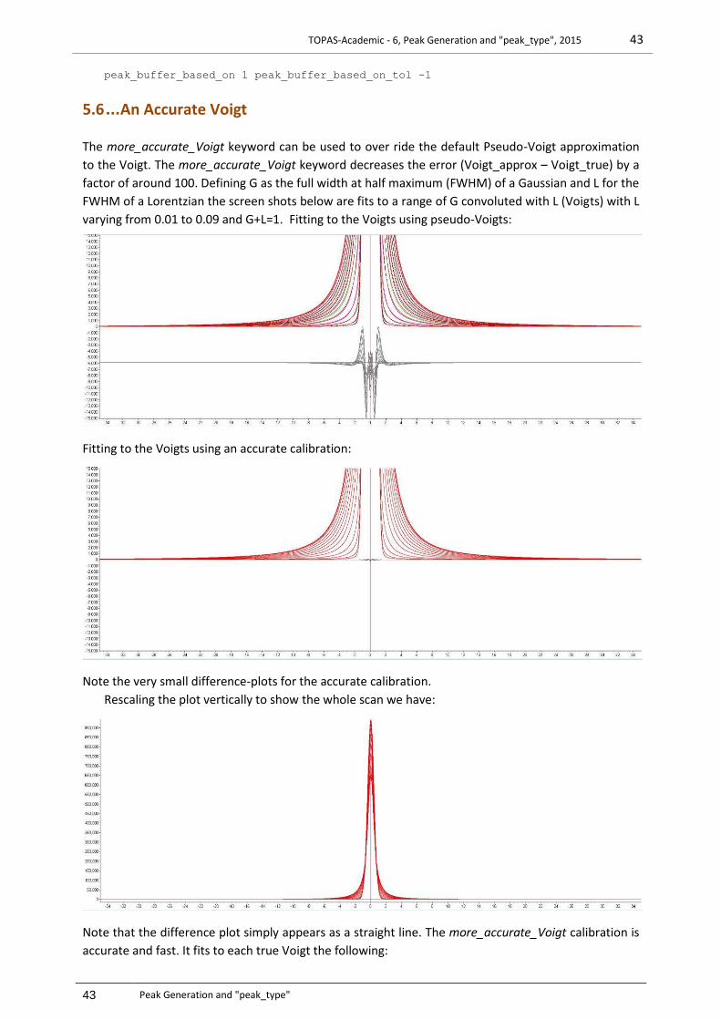
TOPAS-Academic - 6, Peak Generation and "peak_type", 2015 43
43 Peak Generation and "peak_type"
peak_buffer_based_on 1 peak_buffer_based_on_tol -1
5.6 ... An Accurate Voigt
The more_accurate_Voigt keyword can be used to over ride the default Pseudo-Voigt approximation
to the Voigt. The more_accurate_Voigt keyword decreases the error (Voigt_approx – Voigt_true) by a
factor of around 100. Defining G as the full width at half maximum (FWHM) of a Gaussian and L for the
FWHM of a Lorentzian the screen shots below are fits to a range of G convoluted with L (Voigts) with L
varying from 0.01 to 0.09 and G+L=1. Fitting to the Voigts using pseudo-Voigts:
Fitting to the Voigts using an accurate calibration:
Note the very small difference-plots for the accurate calibration.
Rescaling the plot vertically to show the whole scan we have:
Note that the difference plot simply appears as a straight line. The more_accurate_Voigt calibration is
accurate and fast. It fits to each true Voigt the following:
TOPAS-Academic - 6, Peak Generation and "peak_type", 2015 44
44 Peak Generation and "peak_type"
fit_obj = a1 (2 Sqrt(Ln(2) / Pi) / f1) Exp(-4 Ln(2)(X / f1)^2);
fit_obj = a2 (2 Sqrt(Ln(2) / Pi) / f2) Exp(-4 Ln(2)(X / f2)^2);
fit_obj = a3 (2 / (Pi f3)) / (1 + 4 (X / f3)^2);
fit_obj = a4 (4 / (Pi f4)) / (1 + 4 (X / f4)^2)^2;
One thousand sets of a0,a1,a2,a3,f0,f1,f2,f3 parameters were determined by fitting to 1000 true
Voigts with L varying from 0 to 1 in steps of 0.001.
The CREATE.INP file in the TEST_EXAMPLES\VOIGT-APPROX\ directory creates a true Voigt. It uses
the keyword numerical_lor_gauss_conv. The amount of Lorentzian is entered as a number out of a
1000. A number of 500 say would yield a Voigt with a Laurentzian FWHM of 0.5 and a Gaussian FWHM
of 0.5. The generated true Voigt is calculated by numerically convoluting a lor_fwhm with a
gauss_fwhm. The generated true Voigt is saved to a file with the name voigtNNNN.xy, where NNNN
corresponds to a number between 0 and 1000. The file generated contains 100,000 data points. The
step size used in the convolutions is as small as 0.0005 when using a convolution_step of 4.
TOPAS uses an FFT to actually perform the double summation of the convolution. However, for lor
> 500, the convolution itself comprises an analytical Lorentzian with a Gaussian comprising straight
line segments. For lor < 500 then an analytical Gaussian is convoluted with a Lorentzian comprising
straight line segments.
The file FIT-PV.INP fits a pseudo-Voigt to the generated true Voigt.
The file FIT-MORE.INP fits to the generated true Voigt using the c++ equivalent of fit_obj’s.
The file FIT-OBJ.INP fits fit_obj's to the generated true Voigt.
The difference plot from FIT-PV.INP is in the order of 500 to 1000 times larger than the difference plot
from FIT-MORE.INP.

TOPAS-Academic - 6, PDF refinement, 2015 45
45 PDF refinement
6 PDF REFINEMENT
PDF patterns are treated as an ‘xdd’. Many keywords used for xdds can also be used in PDF refinement. PDF
patterns can be refined simultaneously with other types of xdd patterns comprising x-ray dependent or x-ray
independent phases or peaks phases. Penalties, restraints and in particular keywords such as rigid,
atomic_interaction, sites_geometry, sites_distance etc… can all be used. Data structure items frequently used in
PDF refinement are:
xdd…
pdf_data
*[scale_phase_X E]…
*[fit_obj]…
[start_X #] [finish_X #]
*[rebin_with_dx_of !E] [rebin_start_x_at !E]
*[weighting !E]
*[Tpdf_convolute]…
str…
*[scale_phase_X E]…
[scale E]
[view_structure]
[rigid]…
[occ_merge $sites]…
[pdf_scale_simple]
*[pdf_zero E]
[pdf_ymin_on_ymax 0.001]
[pdf_info]
*[Tpdf_convolute]…
[pdf_for_pairs $sites_1 $sites_2]…
[pdf_only_eq_0]
*[pdf_gauss_fwhm E]
*[Tpdf_convolute]…
where
Tpdf_convolute
*[pdf_convolute E]…
[min_X !E]
[max_X !E]
[convolute_X_recal !E]
Examples files in directory test_examples\pdf
beq-2.inp
beq-2-create.inp
beq-3.inp
beq-3-create.inp
pdf-1.inp
pdf-2.inp
alvo4\structure-solution-create.inp
alvo4\structure-solution.inp
alvo4\rigid.inp
occ-merge-pbso4\create.inp
occ-merge-pbso4\occ-merge-test.inp
occ-merge-pbso4\occ-merge.inp

TOPAS-Academic - 6, PDF refinement, 2015 46
46 PDF refinement
Data files in directory test_examples\pdf
beq-2.xy
beq-3.xy
alvo4\alvo4.xy
occ-merge-pbso4\pbso4.xy
Keywords with ‘*’ next to them can be a function of the x-axis reserved parameter name X; for PDF data X
corresponds to r.
pdf_data tells the program that the data set is of G(r) type.
Let’s write G(r) as follows:
G(r) = s1 S(r) / r – s2 r
where
r corresponds to the X-axis
s1 and s2 are constants
S(r) are the pairs
pdf_scale_simple tells the program to calculate S(r)/(Np r) only.
pdf_ymin_on_ymax defines the minimum/maximum value for the Gaussians in regards to the x-axis range
calculated for the Gaussians; the default value of 0.001 in typically sufficient.
pdf_for_pairs can be used to select site pairs using the site name; for example:
pdf_for_pairs "V* Al* !O2" *
The ‘!’ character excludes the sequence from the wild card string. Multiple pdf_for_pairs can be defined.
pdf_only_eq_0 informs the parent pdf_for_pairs that only equivalent position 0 is to be considered.
pdf_gauss_fwhm is used to write the width equation for the pairs selected by pdf_for_pairs. If all of the pairs
possible are described by pdf_for_pairs then the associated beq’s are not used and they become redundant. The
user is informed of unused beq’s. Consider the following abbreviated INP segment:
site Al1 ... beq 1
site O1 ... beq 1
pdf_for_pairs Al1 Al1 pdf_only_eq_0 pdf_gauss_fwhm 0.1 ‘ Line A
pdf_for_pairs Al1 O1 pdf_only_eq_0 pdf_gauss_fwhm 0.2 ‘ Line B
pdf_for_pairs Al1 O1 pdf_gauss_fwhm 0.3 ‘ Line C
There are a number of types of interactions with FWHMs as follows:
Al1O1 interactions for equivalent position 0 described using Line B
Al1O1 interactions excluding equivalent position zero described using Line C
O1O1 interactions described using beq’s
pdf_info displays the interactions used in matrix form; for the above INP segment we get:

TOPAS-Academic - 6, PDF refinement, 2015 47
47 PDF refinement
pdf_info
{
- = No pdf_for_pairs defined hence beq's used
0 = pdf_for_pairs defined with pdf_only_eq_0
1 = pdf_for_pairs defined without pdf_only_eq_0
2 = two pdf_for_pairs defined, one with pdf_only_eq_0 and one without pdf_only_eq_0
Al1 -2
O1 2-
}
The matrix is shown in blue. pdf_for_pairs together with beq’s defaults offers great flexibility in describing peak
widths. See PDF-1.INP, PDF-2.INP, BEQ-3.INP.
scale_phase_X can be used to describe Gaussian dampening, for example:
prm damp_fwhm 50 min 1e-6 max 200
prm damp = Gauss(0, damp_fwhm);
scale_phase_X = damp;
6.1.1 Inter and Intra molecule FWHMs
Assigning different interaction types for molecules is done using pdf_for_pairs. For example, to set the bond
lengths for the atom Al1 of AlVO4 (see PDF-2.INP) to a different FWHM for equivalent position 0 the following
could be used:
prm intra_molec 0.01 min 1e-6
pdf_for_pairs Al1 "O1 O2 O3 O4 O5 O6" pdf_only_eq_0
pdf_gauss_fwhm = intra_molec;
The calculated pattern from PDF-2.INP therefore becomes:
Notice the 6 spikes; they correspond to the Al1 bonds which has narrow FWHMs. If we then wanted Al1
bonds that are not equivalent position 0 to be different to the beq’s values then we could use:
prm inter_molec 0.1 min 1e-6
prm intra_molec 0.01 min 1e-6
pdf_for_pairs Al1 "O1 O2 O3 O4 O5 O6" pdf_only_eq_0
pdf_gauss_fwhm = intra_molec;
pdf_for_pairs Al1 "O1 O2 O3 O4 O5 O6"
pdf_gauss_fwhm = inter_molec;
This gives the following calculated pattern where we see the different bonds of Al1.
Calculated G(r) with a molecule with narrow FWHMs
r
7654321
Co
un
ts
450
400
350
300
250
200
150
100
50
0
-50
-100
-150
-200

TOPAS-Academic - 6, PDF refinement, 2015 48
48 PDF refinement
The corresponding output from pdf_info is:
pdf_info
{
- = No pdf_for_pairs defined
0 = pdf_for_pairs defined with pdf_only_eq_0
1 = pdf_for_pairs defined without pdf_only_eq_0
2 = two pdf_for_pairs defined, one with pdf_only_eq_0 and one without pdf_only_eq_0
Al1 ------222222------
Al2 ------------------
Al3 ------------------
V1 ------------------
V2 ------------------
V3 ------------------
O1 2-----------------
O2 2-----------------
O3 2-----------------
O4 2-----------------
O5 2-----------------
O6 2-----------------
O7 ------------------
O8 ------------------
O9 ------------------
O10 ------------------
O11 ------------------
O12 ------------------
}
An exception is thrown if the same interaction is referenced in more than one pdf_for_pairs, for example, the
following will throw an exception as Al1O1 is references twice:
pdf_for_pairs Al1 "O1 O2 O3 O4 O5 O6" pdf_only_eq_0 …
pdf_for_pairs Al1 O1 pdf_only_eq_0 …
The following will not throw an exception:
pdf_for_pairs Al1 "O1 O2 O3 O4 O5 O6" pdf_only_eq_0 …
pdf_for_pairs Al1 O1 …
6.1.2 Instrument Sinc function Sinc-1.INP
In Sinc-1.PDF pdf_convolute is used at the xdd level to convolute a Sinc function into pdf type phases as follows:
Calculated G(r) with a molecule with narrow FWHMs
r
7654321
Co
un
ts600
550
500
450
400
350
300
250
200
150
100
50
0
-50
-100
-150
-200

TOPAS-Academic - 6, PDF refinement, 2015 49
49 PDF refinement
pdf_convolute = Sin(Qmax X+q3)/If(Abs(X)<0.5 Step_Size, If(X<0,-q2,q2), X);
min_X = -conv_max;
max_X = conv_max;
Sinc-1.INP also uses an xo_Is phase defined as:
xo_Is
NoThDependence(0.0001)
xo 10 I @ 100
peak_type pv
pv_lor 0.5
pv_fwhm 2
pdf_convolute operates on pdf type phases only; hence the xo_Is phase is untouched. Note the phase dependent
use of an emission profile as defined in the NoThDependence macro. Multiple pdf_convolute’s can be described
at the global, xdd, str and pdf_for_pairs levels. Note, use of pdf_convolute as a dependent of pdf_for_pairs is
slower than at the other levels; thus where possible use pdf_convolute at non-pdf_for_pairs levels.
6.1.3 Weighting of PDF and 2-Theta type data
PDF and 2-Theta data can be of very different intensities; the xdd_sum keyword can assist in modifying the weighing of data in order to give the patterns approximately similar weights. For example:
xdd file1.xy
xdd_sum !sum1 = Abs(Yobs);
weighting = 1/sum2;
xdd file2.xy
xdd_sum !sum2 = Abs(Yobs);
weighting = 1/sum2;
pdf_data
6.1.4 Test_examples\pdf\BEQ-2.INP
Use Test_examples\pdf\BEQ-2-create.INP to generate a simulated pattern for BEQ-2.INP
BEQ-2.INP
- Comprise the structure of AlVO4
- 3 types of beq parameters
- beq is a function of X (ie. X corresponds to the X-axis which is r) and hence peak widths are
a function of X.
- demonstrates the use of pdf_zero
- demonstrates the use of rebin_with_dx_of and rebin_start_x_at
6.1.5 Test_examples\pdf\BEQ-3.INP
Use Test_examples\pdf\BEQ-3-create.INP to generate a simulated pattern for BEQ-3.INP
BEQ-3.INP
- Demonstrates the use of pdf_for_pairs
6.1.6 Speeding up refinement with rebin_with_dx_of
The step size in PDF data must be of equal size. Also, the start of the x-axis needs to be an integral multiple of
the step size. Increasing the step size in the data speeds up refinement; see BEQ-2.INP. The step size can be
increased using:

TOPAS-Academic - 6, PDF refinement, 2015 50
50 PDF refinement
macro Rebin_Step { 0.015 }
rebin_with_dx_of Rebin_Step rebin_start_x_at Rebin_Step
Rebinning is akin to collecting the data at a larger step size. All data is included with counts after rebinning being
equal to counts before rebinning. esds associated with the data are also rebinned.
rebin_start_x_at can be used to place the start of the data at an integral multiple of the step size. In BEQ-2.INP
parameters such as scale are written in terms of the rebin step size to reflect the fact that the scaling of the data
is changed due to rebinning.
6.1.7 Refining on beq parameters
Modify the BB macro so that it comprises:
macro BB { } ' beq, Insert/remove !
Gives an Rwp plot of:
This type of convergence is indicative of derivatives being calculated correctly. Convergence for coordinates,
occupancies, lattice parameters and pdf_zero are similar.
6.1.8 Structure Solution, Simulated Annealing
test_examples\pdf\alvo4\structure-solution-create.inp creates a simulated pattern for structure-solution.inp.
It’s a simulated annealing refinement with all coordinates starting at zero with anti-bump penalties applied
using:
AI_Anti_Bump(O* , O* , 2.4, 1, 5)
AI_Anti_Bump(Al*, O* , 1.6, 1, 5)
AI_Anti_Bump(Al*, Al*, 2.8, 1, 5)
The correct solution is found as seen in the following:
10095908580757065605550454035302520151050
160
140
120
100
80
60
40
20
Launch Mode: C:\c\t5\test_examples\pdf\beq-2.inp
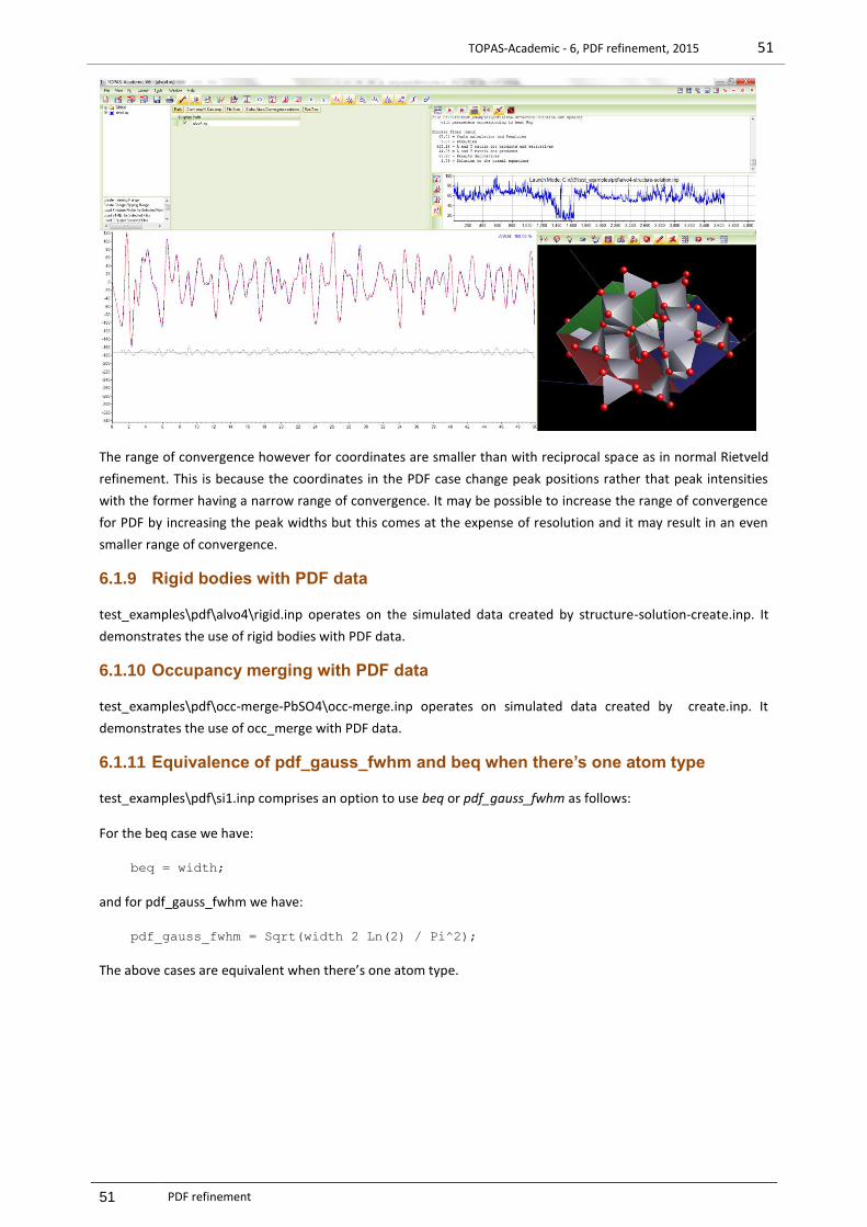
TOPAS-Academic - 6, PDF refinement, 2015 51
51 PDF refinement
The range of convergence however for coordinates are smaller than with reciprocal space as in normal Rietveld
refinement. This is because the coordinates in the PDF case change peak positions rather that peak intensities
with the former having a narrow range of convergence. It may be possible to increase the range of convergence
for PDF by increasing the peak widths but this comes at the expense of resolution and it may result in an even
smaller range of convergence.
6.1.9 Rigid bodies with PDF data
test_examples\pdf\alvo4\rigid.inp operates on the simulated data created by structure-solution-create.inp. It
demonstrates the use of rigid bodies with PDF data.
6.1.10 Occupancy merging with PDF data
test_examples\pdf\occ-merge-PbSO4\occ-merge.inp operates on simulated data created by create.inp. It
demonstrates the use of occ_merge with PDF data.
6.1.11 Equivalence of pdf_gauss_fwhm and beq when there’s one atom type
test_examples\pdf\si1.inp comprises an option to use beq or pdf_gauss_fwhm as follows:
For the beq case we have:
beq = width;
and for pdf_gauss_fwhm we have:
pdf_gauss_fwhm = Sqrt(width 2 Ln(2) / Pi^2);
The above cases are equivalent when there’s one atom type.
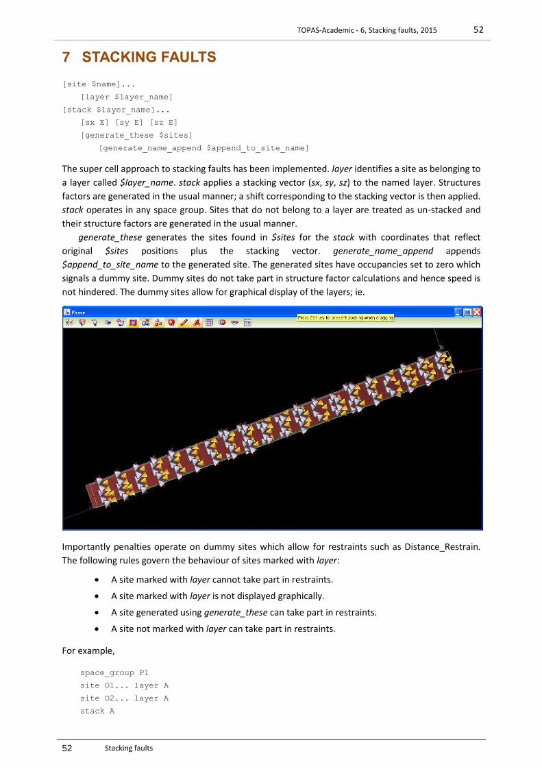
TOPAS-Academic - 6, Stacking faults, 2015 52
52 Stacking faults
7 STACKING FAULTS
[site $name]...
[layer $layer_name]
[stack $layer_name]...
[sx E] [sy E] [sz E]
[generate_these $sites]
[generate_name_append $append_to_site_name]
The super cell approach to stacking faults has been implemented. layer identifies a site as belonging to
a layer called $layer_name. stack applies a stacking vector (sx, sy, sz) to the named layer. Structures
factors are generated in the usual manner; a shift corresponding to the stacking vector is then applied.
stack operates in any space group. Sites that do not belong to a layer are treated as un-stacked and
their structure factors are generated in the usual manner.
generate_these generates the sites found in $sites for the stack with coordinates that reflect
original $sites positions plus the stacking vector. generate_name_append appends
$append_to_site_name to the generated site. The generated sites have occupancies set to zero which
signals a dummy site. Dummy sites do not take part in structure factor calculations and hence speed is
not hindered. The dummy sites allow for graphical display of the layers; ie.
Importantly penalties operate on dummy sites which allow for restraints such as Distance_Restrain.
The following rules govern the behaviour of sites marked with layer:
A site marked with layer cannot take part in restraints.
A site marked with layer is not displayed graphically.
A site generated using generate_these can take part in restraints.
A site not marked with layer can take part in restraints.
For example,
space_group P1
site O1... layer A
site O2... layer A
stack A

TOPAS-Academic - 6, Stacking faults, 2015 53
53 Stacking faults
sx...
generate_these O1
generate_name_append _1
append_fractional
in_str_format
will output for append_fractional the following:
site O1 ...
site O2...
site O1_1 ... occ O 0
The test_examples\stacking-faults\kaolinite.inp shows how to simplify the setting up of layers with
the use of simple macros. Speed of calculation for structure factors are very fast and the derivatives of
the stacking vectors { sx,sy, sz } are very fast. The main bottle neck in speed is summing the peaks to
Ycalc. The switch “#define Speed” in kaolinite.inp shows keywords that can speed things up in the
early stages of determining the stacking vectors.
7.1 ... Fitting to a Debye-formulae generated pattern using ‘stack’
A test pattern was generated using the Debye scattering equation. The structure comprised a single
atom in an Orthorhombic unit cell with 40 layers (40x40x40 unit cells) in the a-b plane shifted
according to {Round(Rand(0,2))/3, Round(Rand(0,2))/3, 0}. The blue line in the following is the
generated pattern comprising the average of 30 runs of the Debye scattering equation. The red line
corresponds to a Rietveld fit of 6 super cell structures (1x1x40) showing that the super cell approach is
a good approximation to the Debye formulae for this example.
The example stacking-faults\debye-new.inp corresponds to the Rietveld fit using the layer and stack
keywords. The debye-old.inp file corresponds to the same Rietveld fit but without the layer and stack
keywords; instead layers are explicitly defined using site in an enlarged unit cell.
There are two time consuming bottle necks dealt with:
1) Summing peaks to Ycalc
2) Calculating structure factors for the stacked layers
The new phase dependent keyword called [del_approx #] groups peaks from the peaks buffer whilst
summing peaks to Ycalc; the peaks are grouped such that their 2Th positions all lie within:
787674727068666462605856545250484644424038363432302826242220181614121086
12,500
12,000
11,500
11,000
10,500
10,000
9,500
9,000
8,500
8,000
7,500
7,000
6,500
6,000
5,500
5,000
4,500
4,000
3,500
3,000
2,500
2,000
1,500
1,000
500
0
-500
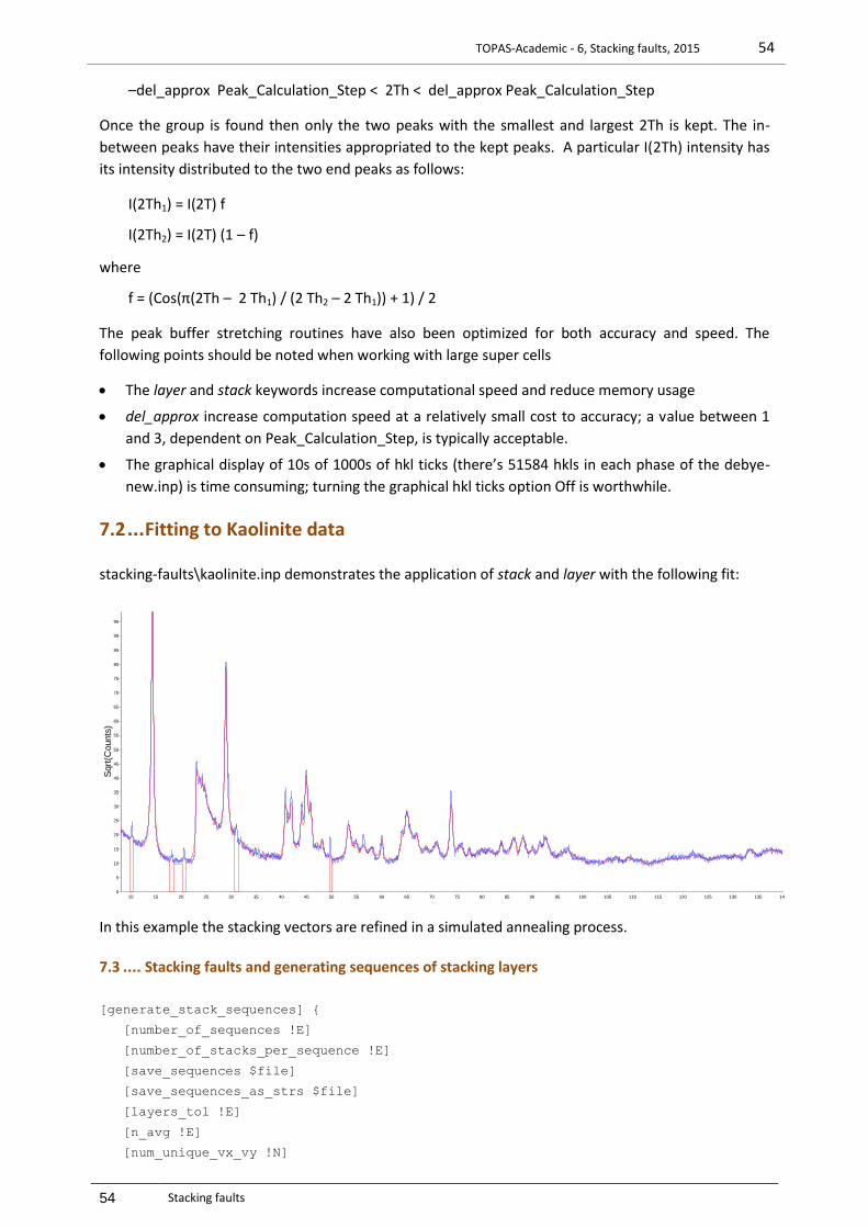
TOPAS-Academic - 6, Stacking faults, 2015 54
54 Stacking faults
–del_approx Peak_Calculation_Step < 2Th < del_approx Peak_Calculation_Step
Once the group is found then only the two peaks with the smallest and largest 2Th is kept. The in-
between peaks have their intensities appropriated to the kept peaks. A particular I(2Th) intensity has
its intensity distributed to the two end peaks as follows:
I(2Th1) = I(2T) f
I(2Th2) = I(2T) (1 – f)
where
f = (Cos(π(2Th – 2 Th1) / (2 Th2 – 2 Th1)) + 1) / 2
The peak buffer stretching routines have also been optimized for both accuracy and speed. The
following points should be noted when working with large super cells
The layer and stack keywords increase computational speed and reduce memory usage
del_approx increase computation speed at a relatively small cost to accuracy; a value between 1
and 3, dependent on Peak_Calculation_Step, is typically acceptable.
The graphical display of 10s of 1000s of hkl ticks (there’s 51584 hkls in each phase of the debye-
new.inp) is time consuming; turning the graphical hkl ticks option Off is worthwhile.
7.2 ... Fitting to Kaolinite data
stacking-faults\kaolinite.inp demonstrates the application of stack and layer with the following fit:
In this example the stacking vectors are refined in a simulated annealing process.
7.3 .... Stacking faults and generating sequences of stacking layers
[generate_stack_sequences] {
[number_of_sequences !E]
[number_of_stacks_per_sequence !E]
[save_sequences $file]
[save_sequences_as_strs $file]
[layers_tol !E]
[n_avg !E]
[num_unique_vx_vy !N]
140135130125120115110105100959085807570656055504540353025201510
Sqrt
(Counts
)
95
90
85
80
75
70
65
60
55
50
45
40
35
30
25
20
15
10
5
0
TOPAS-Academic - 6, Stacking faults, 2015 55
55 Stacking faults
[match_transition_matrix_stats { ... }]
[transition $transition_name]...
[use_layer $layer]
[height E]
[n !N]
[to $to_transition_name !E]...
[ta E] [tb E] [tz E]
[a_add E] [b_add E] [z_add E]
}
' Get(generated_c)
Examples:
test_examples\stacking_faults\
fit-1.inp
fit-2.inp
fit-3.inp
test_examples\stacking-faults\Rietveld-Generate\
Rietveld-Generate\Create-Sequences.inp
Rietveld-Generate\Rietveld-Generate.inp
Rietveld-Generate\Fit-to-Rietveld-Generated.INP
Rietveld-Generate\Rietveld-Generated-200-2000.xy
Rietveld-Generate\strs-200-2000.txt
Stacking fault generation and refinement can now be performed at speeds that make routine analysis possible.
generate_stack_sequences generates sequences of stacks from the transition matrix described by the transition
keywords. The opening and closing braces of {} corresponds to a block where keywords local to
generate_stack_sequences can be used. Outside of the braces the generate_stack_sequences can’t be used.
Get(generated_c) is updated after generation of the sequences with the average thickness of the sequences. It
can be used to set the c lattice parameter.
num_unique_vx_vy: On termination of refinement the number of unique { sx, sy } stacking vector coordinates is
reported for all layer types.
transition: defines a ‘from’ transition with the name $transition_name. The transition uses the layer defined in
use_layer.
to: defines the to-transition. $to_transition_name must be a defined $transition_name.
n returns the number of transitions generated for the corresponding to to-transition.
height: can be used instead of z_add keywords.
ta, tb: defines the stacking vector x and y coordinates in terms of the crystallographic a and b axes.
a_add, b_add: defines the stacking vector x and y coordinates relative to the previous stacking vector in terms of
the crystallographic a and b axes.
tz: defines stacking vector z coordinate along the crystallographic c axis in Å.
add_z: defines stacking vector z coordinate along the crystallographic c axis in Å relative to the previous stacking
vector.
TOPAS-Academic - 6, Stacking faults, 2015 56
56 Stacking faults
7.3.1 Generating the same stacking sequences each run
To generate the same set of stacking sequences each run the random number generated can be seeded with a
constant seed using seed, for example:
seed #number
#number is a constant integer. Each #number generates its own unique set of random numbers. Generating
identical sets of stacking sequences is useful when changes in Rwp that excludes stacking sequence variation is
required.
7.3.2 The SF_Smooth macro
Stacking faulted calculated patterns can contain ripples when the peak shapes are small or when there’s too few
layers stacked. The SF_Smooth macro, defined in TOPAS.INC smooths out these ripples such that small
supercells can approximate large supercells; this crease computation speed and reduces memory usage. All
stacking fault examples uses SF_Smooth; typical usage is as follows:
SF_smooth(@, 1, 1)
The refined parameter adjust the width of a Gaussian convolution that is dependent on hkls and the intensities
of the reflections. The last argument (the ‘1’) can be used to adjusted the tolerance of a peak_buffer_based_on
keyword used in SF_Smooth. The definition is as follows:
peak_buffer_based_on = idl;
peak_buffer_based_on_tol = Max(0.01 idl, Peak_Calculation_Step 0.5 s);
Reducing s increases the number of peaks in the peaks buffer and increases the accuracy of the calculated
pattern. Typically s=1 is sufficient.
7.3.3 Fitting to DIFFaX test diamond data
Fit-1.INP uses generate_stack_sequences to fit to data generated from the DIFFaX suite (Treacy, 1991); INP
segment that generates the sequences looks like:
generate_stack_sequences {
number_of_sequences Nseqs 200
number_of_stacks_per_sequence Nv 200
num_unique_vx_vy 6
Transition(1, lpc)
to 1 = pa; a_add = 2/3; b_add = 1/3; n !n1 349984
to 2 = 1-pa; a_add = 0; b_add = 0; n !n2 149781
Transition(2, lpc)
to 1 = 1-pa; a_add = 0; b_add = 0; n !n3 149781
to 2 = pa; a_add = -2/3; b_add = -1/3; n !n4 350254
}
The generated probability parameter pa can be determined using the n values as follows:
prm !pa_gen = (n1+n3)/(n1+n2+n3+n4); : 0.699974874
The fit to the DIFFaX data looks like:

TOPAS-Academic - 6, Stacking faults, 2015 57
57 Stacking faults
7.3.4 Stacking faults from layers of different layer heights
Layers of different thicknesses can be modelled accurately and refinement fast. Here’s a fit to simulated data
(FIT-2.INP) for two different layer heights of 5 and 6Å.
7.3.5 Rietveld-Generated example
The files in the test_examples\stacking-faults\Rietveld-Generate\ directory can be used to create a stacking
faulted test pattern using Rietveld refinement. The test pattern can then be fitted to. Create-Sequences.inp
created the INP format stacking sequences and places the result int the file strs-200-2000.txt. The file Rietveld-
Generate.inp can then be used to create the test pattern Rietveld-Generated-200-2000.xy. This test pattern can
be fitted to using the file Fit-to-Rietveld-Generated.INP; this file uses generate_stack_sequences. It
demonstrates the accuracy and speed of the stacking fault averaging fitting procedure. The fit to the Rietveld
generated stacking faulted pattern looks like:
Fit-1.INP, Fitting to DIFFaX test diamond data
2Th Degrees14514013513012512011511010510095908580757065605550454035
Ln
(Co
unts
)2.6
2.5
2.4
2.3
2.2
2.1
2
1.9
1.8
1.7
1.6
1.5
1.4
1.3
1.2
1.1
1
0.9
0.8
0.7
0.6
0.5
0.4
0.3
0.2
0.1
0
-0.1
Fit-2.INP, Fitting to test data created with different layer heights
2Th Degrees145140135130125120115110105100959085807570656055504540353025201510
Sq
rt(C
ou
nts
)
100
95
90
85
80
75
70
65
60
55
50
45
40
35
30
25
20
15
10
5
0
-5
Fit-to-Rietveld-Generated.INP
2Th Degrees3938373635343332313029282726252423222120191817161514131211
Sq
rt(C
ou
nts
)
300
290
280
270
260
250
240
230
220
210
200
190
180
170
160
150
140
130
120
110
100
90
80
70
60
50
40
30
20
10
0

TOPAS-Academic - 6, Stacking faults, 2015 58
58 Stacking faults
7.3.6 Refining on layer heights
Layer heights can be refined by refining on parameters that are a function of the add_z or height keywords. The
Fit-3.INP example refines on 3 height parameters as well as the z fractional atomic coordinates of the sites that
comprise the layers. It also lists six types of transitions which operate on three unique layer types. The
transitions point to the layer types using the use_layer keyword. The c lattice parameter is defined and refined
using the following:
prm qq 0 c = Get(generated_c) + 0.0001 qq; : 1828.085117
Get(generated_c) is also used to initialize the z fractional coordinates of the sites as follows:
prm height_Se01 7.49691 prm !zSe01 = height_Se01/Get(generated_c);
site Se01 x 0.5 y 0 z = zSe01; occ Se 1 beq !bval 1 layer cd00
The fit to the test data looks like:
Fit-3.INP, Refining on stacking vector and structural parameters
2Th Degrees292827262524232221201918171615141312111098765432
Sq
rt(C
ou
nts
)
550
500
450
400
350
300
250
200
150
100
50
0

TOPAS-Academic - 6, Quantitative Analysis, 2015 59
59 Quantitative Analysis
8 QUANTITATIVE ANALYSIS
The following are items associated with quantitative analysis:
xdd..
mixture_MAC
mixture_density_g_on_cm3
weight_percent_amorphous
elemental_composition
element_weight_percent...
element_weight_percent_known...
prm = Get(sum_smvs)...
Mixture_LAC_1_on_cm(0) ' macro
str...
weight_percent
cell_mass
cell_volume
phase_MAC
spiked_phase_measured_weight_percent
corrected_weight_percent
prm = Get(sum_smvs)...
prm = Get(smv)...
prm = Get(sum_smvs_minus_this)...
prm = Get_Element_Weight(atom)...
Phase_LAC_1_on_cm(0) ' macro
Phase_Density_g_on_cm3(0) ' macro
Test_examples\quant\quant-1.inp uses many of these and additionally writes equivalent terms in the
form of equations, for example:
' This is weight_percent
prm = 100 Get(smv) / Get(sum_smvs); : 0
prm q = spiked_phase_measured_weight_percent /
spiked_phase_measured_weight_percent_wt; : 0
' This is corrected_weight_percent
prm = q Get(weight_percent); : 0
' This is weight_percent_amorphous
prm = 100 (1 - q); : 0
8.1 ... Elemental weight percent constraint
The QUANT implementation is almost entirely written internally using the TOPAS Symbolic system.
Dependencies are automatically taken care of and unnecessary recalculations kept to a minimum. The
overriding plus however is the flexibility it allows. If for example an elemental weight percent was
known and three phases of the mixture comprised this element then Get_Element_Weight can be
used to get the weight of the element as a function of the structure; ie.
str...
prm z1 = Get_Element_Weight(Zr);
MVW(!m1 0, !v1 0,0)

TOPAS-Academic - 6, Quantitative Analysis, 2015 60
60 Quantitative Analysis
str...
scale s2 0.001
prm z2 = Get_Element_Weight(Zr);
MVW(0, !v2 0,0)
str...
scale s3 0.001
prm z3 = Get_Element_Weight(Zr);
MVW(0, !v3 0,0)
Rearranging the formulae for element weight percent, the scale parameter of one of the phases, say
the first one, can be written as follows:
scale = (0.01 known_Zr Get(sum_smvs_minus_this) - s2 v2 z2 - s3 v3 z3) / (v1 (z1
- 0.01 known_Zr m1));
Get(sum_smvs_minus_this) returns the sum of SMVs minus the phase where it is defined. The
test_example\quant\quant-3.inp demonstrates this constraint with very good convergence. It
comprises 4 phases with three of them comprising Zr atoms. Quant-2.inp demonstrates constraining a
weight percent to a known value using the macro:
macro Known_Weight_Percent(& w) {
scale =(w/(100-w)) Get(sum_smvs_minus_this)/(Get(cell_mass) Get(cell_volume));
}
8.2 ... Elemental composition and Restraints
The xdd dependent keyword element_composition reports the elemental composition for atoms
within the structures of the xdd, for example:
Before Refinement:
xdd...
elemental_composition
After Refinement:
xdd...
elemental_composition
{
Rietveld
AL 0.875`_0.021
O 26.135`_0.009
SI 0.090`_0.003
Y 6.289`_0.012
ZR 66.612`_0.029
}
element_weight_percent $ELEMENT $NAME #: is an xdd dependent keyword that returns the weight
percent of an element within the corresponding str’s of the xdd. Example usage:
Before Refinement:
penalties_weighting_K1 .1
xdd...
element_weight_percent Zr+4 zr 0
restraint = (zr - 65); : 0

TOPAS-Academic - 6, Quantitative Analysis, 2015 61
61 Quantitative Analysis
After Refinement:
penalties_weighting_K1 .1
xdd...
element_weight_percent Zr+4 zr 65.0275252`
restraint = (zr - 65); : 0.0275251892`
In this example zr is the name given to the element Zr+4 and the restraint shows a known value of 65
(set for example by XRF results). The refinement obeys the restraint according to the value set for
penalties_weighting_K1.
For restraining a weight percent the following can be used:
xdd...
penalties_weighting_K1 .2
restraint = (Cubic_Zirconia_wt_percent - 36); : 0
str...
MVW(0,0, !Cubic_Zirconia_wt_percent 0)
Note, the Cubic_Zirconia_wt_percent name which is given to the weight percent; see test
examples\quant.
8.3 ... Amorphous phase composition
If spiked_phase_measured_weight_percent is defined then elemental_composition will report on
Rietveld values, Corrected values as well as values from the original un-spiked sample. If
element_weight_percent_known keywords are defined then elemental_composition will additionally
report on the elemental contents of the amorphous phase, for example, from
test_examples\quant\quant-1.inp we have:
elemental_composition
{
Rietveld Corrected Original Other
AL 1.176`_0.042 1.059`_0.000 0.000`_0.000 0.000`_0.000 O 26.271`_0.017 23.640`_0.832 23.162`_0.849 0.838`_0.849
SI 0.104`_0.004 0.094`_0.005 0.096`_0.005 0.000`_0.000
Y 6.182`_0.013 5.563`_0.204 5.676`_0.209 0.000`_0.000
ZR 66.267`_0.055 59.631`_2.185 60.847`_2.229 2.153`_2.229
Other 0.000`_0.000 10.015`_3.224 10.219`_3.290 7.228`_0.212 }
The first second and third columns sum to 100%. The second column corresponds to corrected values
including the spiked phase. The third and fourth columns relate to elemental weight percents of the
original phase. The last row of the second column (in purple) corresponds to
Get(weight_percent_amorphous), the last row of the fourth column (in red) is the amount that is
undefined; it comprises the Green number minus the elements of the third column excluding the last
row. Note the zeros for Al (in blue); this is due to the spiked phase (dummy test data) being the only
phase containing Al.
8.4 ... Using a dummy_str phase to describe amorphous content
If it is known that the amorphous content, (purple number) in the above table comprises a known
composition, say TiO2, then a dummy_str can be used to describe the amorphous content as follows:
dummy_str
phase_name "Amorphous"
a 5 b 5 c 5
space_group 1

TOPAS-Academic - 6, Quantitative Analysis, 2015 62
62 Quantitative Analysis
site Ti occ Ti 1
site O occ O 2
Known_Weight_Percent(10.0148)
MVW(0, 0 ,0)
*** Note: dummy_str’s void of MVW and sites takes no part in Quantitative analysis. The lattice
parameters and the chemistry should correspond to a real structure in order for
Mixture_LAC_1_on_cm and phase_LAC to be correctly calculated; in the case of using the Brindley
correction these changed values will change the quantitative results. The space group entry can be
other than P1 so long as the chemistry is correct. Inclusion of the dummy_str produces:
elemental_composition
{
Rietveld Corrected Original
AL 1.059`_0.038 1.059`_0.000 0.000`_0.000
O 27.652`_0.015 27.652`_0.975 27.256`_0.995
SI 0.094`_0.003 0.094`_0.005 0.096`_0.005
TI 6.002`_0.000 6.002`_0.215 6.125`_0.219
Y 5.563`_0.012 5.563`_0.204 5.676`_0.209
ZR 59.631`_0.050 59.631`_2.185 60.847`_2.229
Other 0.000`_0.000 0.000`_3.583 0.000`_3.656
}
Note that the ‘Other’ row becomes zero as the dummy_str has been assigned the amorphous content.
The change in mixture values are:
Without dummy_str
Mixture_LAC_1_on_cm( 557.47740`_0.58665)
mixture_density_g_on_cm3 5.26713308`_0.00292681843
With dummy_str
Mixture_LAC_1_on_cm( 608.85143`_0.76954)
mixture_density_g_on_cm3 5.86601008`_0.00407998952
If XRF results were entered for element_weight_percent_known, for example:
element_weight_percent_known Zr 63
element_weight_percent_known O 24
Then we get:
elemental_composition
{
Rietveld Corrected Original Other
AL 1.059`_0.038 1.059`_0.000 0.000`_0.000 0.000`_0.000
O 27.652`_0.015 27.652`_0.975 27.256`_0.995 -3.256`_0.995
SI 0.094`_0.003 0.094`_0.005 0.096`_0.005 0.000`_0.000
TI 6.002`_0.000 6.002`_0.215 6.125`_0.219 0.000`_0.000
Y 5.563`_0.012 5.563`_0.204 5.676`_0.209 0.000`_0.000
ZR 59.631`_0.050 59.631`_2.185 60.847`_2.229 2.153`_2.229
Other 0.000`_0.000 0.000`_3.583 0.000`_3.656 1.103`_0.431 }
The negative element weight percent for O for the amorphous content reflects the fact that the
measured XRF value for O is lower than the refinement’s value (note, this example is simply for testing
and the XRF values used are fictitious).
8.5 ... Quant using hkl_Is or other non-str phases
dummy_str’s can be used to represent the quantitative results arising from non-str phases. For
example, consider a phase where the structure is unknown but the chemistry is known and a
calibration constant has been determined relating the hkl_Is intensities to the scale parameter of the
hkl_Is phase. In such a case the dummy_str can be written as (see Quant-6.inp):

TOPAS-Academic - 6, Quantitative Analysis, 2015 63
63 Quantitative Analysis
dummy_str
phase_name "Linked Cubic Zirconia"
Cubic(5.137866)
space_group F_M_-3_M
site Zr x 0 y 0 z 0 occ Zr 0.85
occ Y 0.15
site O x 0.25 y 0.25 z 0.25 occ O 0.962
scale = hkl_scale;
Phase_LAC_1_on_cm(0)
Phase_Density_g_on_cm3(0)
MVW(0, 0 ,0)
Note in this case a space group has been entered with structural parameters that looks like a known
structure; this could occur for example where the structure is known in an ordered state but the
diffraction pattern comprises a disordered state. In other cases the P1 space group may suffice with
site occupancies corresponding to the appropriate chemistry. The dummy_str is linked to the hkl_Is
phase by assigning it scale parameter to the hkl_Is scale parameter. Quant-7.inp is a similar process
except that a fit_obj is linked to a dummy_str. Graphically the linked dummy_str is plotted with the
calculated pattern of the hkl_Is phase or fit_obj, for example, Quant-7.inp produces:
Here the Blue line corresponds to the dummy_str which plots the calculated pattern of the linked
fit_obj which in turn comprises a user_y object. The weight percent value determined by the
dummy_str is also displayed.
8.6 ... Summary of Quant examples
Quant-1.inp: a general example showing the use of element_weight_percent_known etc...
Quant-2.inp: uses the Known_Weight_Percent macro
Quant-3.inp: uses elemental constrain using Get_Element_Weight
Quant-4.inp: uses an hkl_Is phase instead of a str phase; uses Known_Weight_Percent on the
hkl_Is phase.
Quant-5.inp: uses a dummy_str to describe an amorphous phase
Quant-6.inp: uses a hkl_Is phase to describe a phase; links a dummy_str to the hkl_Is phase to get
QUANT info.
Quant-7.inp: uses a fit_obj that is a function of a user_y object to describe a phase; links a
dummy_str the fit_obj to get QUANT info.
120118116114112110108106104102100989694929088868482807876747270686664626058565452504846444240383634323028262422201816
210
200
190
180
170
160
150
140
130
120
110
100
90
80
70
60
50
40
30
20
10
0
-10
-20
Linked Cubic Zirconia 48.24 %
Zircon 0.55 %
Zr O2 49.40 %
Corundum Al2 O3 1.81 %

TOPAS-Academic - 6, Quantitative Analysis, 2015 64
64 Quantitative Analysis
8.7 ... External standard method
The method of O’Connor and Raven (1988) has been implemented in both GUI and Launch modes
through the use of the macros:
macro K_Factor_MAC_K(mac, k, tot) {
move_to xdd
local !k_factor_mac_local_ mac
local !k_factor_k_local_ k
local !k_factor_sum_wps_ = 0; : tot
}
macro K_Factor_WP(result) {
local k_factor_wp_ = 1.6605402 Get(smv) k_factor_mac_local_ /
k_factor_k_local_; : result
if Prm_There(k_factor_sum_wps_) {
existing_prm k_factor_sum_wps_ += k_factor_wp_;
}
}
See test_examples\k-factor.

TOPAS-Academic - 6, Magnetic Structure Refinement, 2015 65
65 Magnetic Structure Refinement
9 MAGNETIC STRUCTURE REFINEMENT
str...
[mag_only_for_mag_sites]
[mag_space_group $symbol]
site...
[mlx E] [mly E] [mlz E] [mg E]
[mag_only]
' site dependent macros
MM_CrystalAxis_Display(mxc, myc, mzc)
MM_CrystalAxis_Refine(mxc,mxv,myc,myv,mzc,mzv,mlx_v,mly_v,mlz_v)
MM_Cartesian_Display(mxc, myc, mzc)
MM_Cartesian_Refine(mxc,mxv,myc,myv,mzc,mzv,mlx_v,mly_v,mlz_v)
Thanks to Branton Campbell and John Evans for expert assistance during the implementation of
magnetic refinement. Magnetic refinement is implemented using the keywords mlx, mly, mlz, mg and
mag_space_group. See example in the test_examples\mag directory as well as the tutorial by John
Evans at http://www.dur.ac.uk/john.evans/topas_workshop/tutorial_lamno3_magnetic.htm.
The Magnetic intensity is given by:
Magnetic intensity = Fmagcperp . Fmagcperp* = |Fmagcperp|
where the superscript * denotes conjugate gradient and:
Fmagcperp = Fmagc - (Fmagc . Qhat) Qhat
Or in words, Fmagcperp is the component of the magnetic vector in the direction perpendicular to the
scattering vector Q, where
Q = (L-1)T * h
Qhat = Q / |Q|
where
L is the Cartesian lattice parameters in 3x3 matrix form
h is the Miller indices in vector form
* denotes matrix multiplication
Superscript -1 denotes matrix inverse
Superscript T denotes matrix transpose
(L-1)T = reciprocal lattice parameters
Fmagc in terms of the Cartesian lattice parameters is:
Fmagc = L * Fmag
Fmag for the plane h for a single site is:
Fmag = ∑j (Bj * m) Exp(2π i Uj)
where the summation is over the equivalent positions j and
Uj = h.Rj x + h.tj
x = { x, y, z } = site fractional coordinates
m = { mlx, mly, mlz } = magnetic moment

TOPAS-Academic - 6, Magnetic Structure Refinement, 2015 66
66 Magnetic Structure Refinement
Rj = rotation part of space group operator
tj = translational part of space group operator
dj = sj determinant(Rj) = sj det(Rj)
Bj = sj det(Rj) Rj = magnetic transformation matrix
The file MAGDATA.DAT (a GSAS file - permission for its use granted from Robert Von Dreele, the
author of GSAS) comprises data for calculating magnetic form factors. The Lande splitting factor can
be refined using the site dependent parameter mg; defaults for mg are obtained from MAGDATA.DAT.
Shubnikov groups are obtained from the file SHUBNIKOVGROUPS.TXT.
mag_only: When defined the x-ray component to intensity for the site in question is ignored.
mag_only_for_mag_sites: When defined the x-ray component to intensity for all magnetic sites for
the str in question is ignored.
9.1 ... Magnetic refinement warnings/exceptions
The following two messages:
1) Warning: Magnetic moment mlx of site Fe has no contribution to Fmag
2) Magnetic moment mlx of site Fe cannot be refined as it has no derivative
arise when for each group of equivalent positions of a special position the first row of the matrix
∑jBj*m is zero where the j’s sum over the equivalent positions of a special position group. Similar
messages for mly and mlz are given. Note, the fact that mlx, mly, mlz may or may not be refined and
their associated constraints are considered. Refinement terminates in the case of message (2) when
mlx is being refined.
9.2 ... Displaying Magnetic moments
Magnetic moments (Occupancy Bj*m) are displayed graphically when ‘view_structure’ is defined. For
the case where the atom balls are masking the display of the magnetic moment arrows the “Atom
size” can be varied as shown in the following:

TOPAS-Academic - 6, Magnetic Structure Refinement, 2015 67
67 Magnetic Structure Refinement
9.3 ... ‘Decomposing’ Fmag for speed
When using magnetic space groups, equivalent positions for space groups other than 1.1 are written
in terms of other equivalent positions.
Let Cj = cos(Uj)
Sj = sin(Uj)
Exp( i U) = Cj + i Sj = Euler's formulae
For two equivalent positions of a special position we have
U1 = U2 = U
Fmag1+Fmag2 = s1 det(R1) R1 m Exp(i U) + s2 det(R2) R2 m Exp(i U)
= (s1 det(R1) R1 + s2 det(R2) R2) m Exp(i U)
= c m Exp(i U)
c is independent of x
Note, a particular special position could have many equivalent positions.
If R1 = -R2 and t1 = -t2 for two equivalent positions then
U1 = -U2 = U
Fmag1+Fmag2 = s1 det(R) R m Exp(i U) + s2 det(-R) (-R) m Exp(-i U)
Now,
det(R) R = det(-R) (-R)
or, Fmag1+Fmag2 = det(R) R m (s1 Exp(i U) + s2 Exp(-i U))
For s1 = s2, Fmag1+Fmag2 = s1 det(R) R m 2 C
For s1 = -s2, Fmag1+Fmag2 = s1 det(R) R m (2 i S)
If R1 = R2 for two equivalent positions then
Fmag1+Fmag2 = s1 det(R) R m Exp(i h. R x) Exp(i h.t1) + s2 det(R) R m Exp(i h. R x) Exp(i h.t2)
= det(R) R m (s1 Exp(i h.t1) + s2 Exp(i h.t2)) Exp(i h. R x)
= c Exp(i h. R x)
c is independent of x and is calculated only once.
Many R's can be the same for a particular space group with only the t's changing.
Calculating C and S
Exp(i (h . R x + h. t)) = Exp(i h . R x) Exp( i h . t)
Exp(i h . t) is constant for a particular h and is calculated only once.
Only unique Exp(i h . R x) are calculated.
Trigonometric recurrence is used to calculate sines and cosines resulting in three cosine and three
sine operations per unique equivalent r. In other words a sin and cos is not calculated for each h.
Note a sin or cos function is equivalent to about 40 to 60 multiplies.

TOPAS-Academic - 6, Miscellanous, 2015 68
68 Miscellanous
10 MISCELLANOUS
10.1 Threading
TOPAS is threaded to a large extent; this allows the utilization of multiple processors which results in faster
program execution. The degree of speedup is computer and problem dependent. For non-trivial problems the
gain is 2 to 4 for a 4 core laptop PC with four i7 processors as seen in the following table.
Time (secs) Gain
INP File Comment V6 V5 V4 V4/V6 V5/V6
\ft\alvo4a "#define TEST_ #define USE_FT_
#define USE_SH_" ft, spherical harmonics 1.70 6.75 - - 3.97
\absorption-edge\Al2O3-pam Absorption edge, modify peak 1.46 5.67 - - 3.87
\cime-z-auto "#define TEST_2_" no decompose 7.08 25.03 18.70 2.64 3.54
\tof\tof_bank2_2 user_defined_convolution 0.18 0.63 0.53 2.93 3.49
\wppm\cube-ln-normal-1 "#define TEST_" 2.34 8.05 - - 3.44
\alvo4a "#define TEST_" 1.22 3.95 5.52 4.52 3.24
\single-crystal\ae14-approx-a "#define TEST_" 1.03 3.31 11.47 11.14 3.21
\mag\mag "#define TEST_" 1.09 3.20 - - 2.94
\single-crystal\pn_02_2-adps 3970 parameters 6.32 17.37 27.88 4.41 2.75
\single-crystal\ae14-adps 0.29 0.78 1.27 4.46 2.73
\li250 0.39 1.06 0.81 2.08 2.72
\tube-tails "#define TEST_" 1.48 3.80 3.20 2.16 2.56
\pbso4a "#define TEST_" 2.29 5.74 6.42 2.80 2.50
\single-crystal\pn_02_2 "#define TEST_1_" 3.23 8.01 11.73 3.63 2.48
\sp\serine_I_evans_N_ta_bang_rot-z z-matrix 0.67 1.62 2.35 3.51 2.41
\ft\alvo4a "#define TEST_ #define USE_FT_" ft, no spherical harmonics 0.38 0.91 - - 2.38
\ft\alvo4a "#define TEST_" no ft, no spherical harmonics 0.21 0.48 - - 2.29
\single-crystal\ae14-adps "#define TEST_" no approximate_A 0.57 1.31 5.74 10.04 2.29
\capillary-lpsd\capillary-simulated 0.10 0.22 - - 2.28
\y2o3a 0.24 0.54 0.44 1.82 2.25
\peak-intensity-extraction\zhu3lebail 0.16 0.34 0.49 3.14 2.20
\sp\serine_I_evans_N_ta_bang_rot-z 0.82 1.79 2.28 2.78 2.18
\Voigt-approx\fit-obj.inp "#define TEST_" 4.39 9.55 - - 2.18
\zro2 "#define TEST_" 1.87 3.82 - - 2.05
\cime-z-auto "#define TEST_1_" decompose 6.95 13.87 15.20 2.19 2.00
\k-factor\k-factor 0.33 0.64 - - 1.95
\single-crystal\pn_02_2 "#define TEST_2_" no approximate_A 25.68 49.30 97.15 3.78 1.92
\mag\JohnEvans\jsoe_fit_p1_tofullproftric_0
1 "macro aac$ { iters 30 }" 4.00 7.61 - - 1.90
\peak-intensity-extraction\pawley1 "#define
TEST_" 1.73 3.16 3.98 2.30 1.83
\cf\cf-1a7y “#define TEST_” Charge Flipping 12.87 23.40 25.81 2.00 1.81
\ft\alvo4a "#define TEST_ #define USE_SH_" no ft, spherical harmonics 0.53 0.95 - - 1.79
\sp\serine_i_evans_n_ta_bang_rot 0.74 1.27 1.90 2.57 1.71
\pvs "#define TEST_" 1.22 2.08 4.94 4.05 1.70
\stacking-faults\kaolinite "#define TEST_1_
#define Speed" with Speed 0.58 0.97 - - 1.66
\stacking-faults\kaolinite "#define TEST_1_" 3.10 4.96 - - 1.60
TOPAS-Academic - 6, Miscellanous, 2015 69
69 Miscellanous
\clay 0.75 1.15 2.90 3.87 1.53
\tof\tof_bank2_1 "#define TEST_" 0.60 0.92 2.28 3.80 1.53
\occ-merge "#define TEST_" 3.37 4.90 6.20 1.84 1.45
\simon\alan Many smalll strs 0.73 0.97 3.36 4.60 1.33
Attention has been paid to reducing memory usage at the thread level. This is particularly apparent when using
rigid bodies or occupancy merge where Version 6 uses far less memory than Version 5. Except for penalties all
items are threaded and they include:
- Peak generation
- All colvolutions
- All derivatives that are a function of Ycalc
- Equations that are a function of changing variables such as X, Th, D_spacing etc...
- Pawley refinement
- Strucure refienment
- Charge Flipping
- Magnetic refinement
- Stacking faults
- PDF refinement
- Conjugate gradient solution method
- Indexing
10.1.1 ....Setting the maximum number of threads - MaxNumThreads.TXT
The maximum number threads available is used by default. The user can limit the maximum number of
threads by editing the file MaxNumThreads.TXT. This file is read on porgram startup; it contains a
single number, lets call it Max_Threads_File, which defines the maximum number of threads. Non-
existance of the file or a Max_Threads_File of zero results in the porgram using the maximum number
of threads available. If Max_Threads_File is negative then the maximum number of threads is set to the
following:
Max_Number_Threads = Max(1, Max_Threads_File + Max_Threads_Available);
10.2 . Calculation of structure factors
The structure factor F for a particular reflection (h k l) is the complex quantity:
F = s (AS + i BS) a (fo,a + fa' + i fa
") Oa (10-1)
The summation s is over the sites of the unit cell and the summation a is over the atoms residing on
site s. Oa and fo,a corresponds to the site occupancy and the atomic scattering factor for atom ’a’
respectively. fa' and fa" are the anomalous dispersion coefficients for atom ’a’. AS and BS corresponds to
the cosine and sine summations for site 's', or:
AS = e Ts,e cos(2 h . re), BS = e Ts,e sin(2 h . re) (10-2)
where Ts,e is the temperature factor and the summation e is over the equivalent positions of site 's' as
dictated by the space group. Defining:

TOPAS-Academic - 6, Miscellanous, 2015 70
70 Miscellanous
fo,s = a fo,a Oa, fs' = a fa
' Oa, fs" = a fa
" Oa (10-3)
and separating the real and imaginary components gives:
F = s (As + i Bs) (fo,s + fs'+ i fs
")
F = s (As (fo,s +fs') Bs fs
") + i s (As fs" + Bs (fo,s + fs
'))
or, F = A + i B
(10-4)
The observed intensity is proportional to the complex conjugate of the structure factor, or,
F2 = A2 + B2 (10-5a)
or,
F2 = A012 + B01
2 + A112 + B11
2 + 2 B01 A11 - 2 A01 B11 (10-5b)
where A01= s As (fo,s + fs'), A11 = s As fs
"
B01= s Bs (fo,s + fs'), B11 = s Bs fs
"
and A = A01 B11, B = B01 + A11
Atomic scattering factors used, fo,a, are by default those from
http://www.esrf.fr/computing/expg/subgroups/theory/DABAX/dabax.html
these comprise 11 values per atom and are found in the file ATMSCAT_11.CPP. Correspondingly 9
values per atom, obtained from the International Tables, are found in the file ATMSCAT_9.CPP. Use of
either 9 or 11 values can be invoked by running the batch files use_9f0 and use_11f0 respectivelly.
Dispersion coefficients used, fa' and fa
", are by default from
http://www.cxro.lbl.gov/optical_constants/asf.html
These data, found in the SSF directory, covers the energy range from 10 to 30000eV. The use of
use_tube_dispersion_coefficients forces the use of dispersion coefficients from the International Tables
for X-ray Crystallography [1995], Vol.C, p384-391 and 500-502, and for O2- from Hovestreydt [1983].
These data are in discrete energy steps corresponding to wavelengths typically found in laboratory X-
ray tubes.
For neutron diffraction data fa'= fa
"=0 and fo,a is replaced by the bound coherent scattering length
(found in the NEUTSCAT.CPP file) for atom ‘a’ obtained from
http://www.ccp14.ac.uk/ccp/web-mirrors/neutrons/n-scatter/n-lengths/LIST~1.HTM
10.2.1 ....Friedel pairs
For centrosymmetric structures the intensities for a Friedel reflection pair are equivalent, or, F2(h k l) =
F2(-h-k-l). This holds true regardless of the presence of anomalous scattering and regardless of the
atomic species present in the unit cell. This equivalence in F2 is due to the fact that B01 = B11 = 0 and
thus:
F = A01 + i A11 and F2 = A012 + A11
2 (10-6)

TOPAS-Academic - 6, Miscellanous, 2015 71
71 Miscellanous
For non-centrosymmetric structures and for the case of no anomalous scattering, or for the case
where the unit cell comprises a single atomic species, then F2(h k l) = F2(-h-k-l). Or, for a single atomic
species we have:
B01 A11 = (f0 +f') (S BS) f" (S AS), A01 B11 = (f0 +f') (S AS) f
" (S BS)
or, B01 A11 = A01 B11
(10-7)
and thus from cancellation in Eq. (10-5b) we get
F2(h) = F2(-h) = A012 + B01
2 + A112 + B11
2 (10-8)
For non-centrosymmetric structures and for the case of anomalous scattering and for a structure
comprising more than one atomic species then F2(h) F2(-h).
10.2.2 ....Powder data
Friedel pairs are merged for powder diffraction data meaning that the multiplicities as determined by
the hkl generator includes the reflections (h k l) and (-h -k -l); this merging of Friedel pairs improves
computational efficiency. Eq. (10-5b) gives the correct intensity for unmerged Friedel pairs and thus it
cannot be used for merged Friedel pairs. Using the fact that:
A01(h) = A01(-h), A11(h) = A11(-h)
B01(h) = B01(-h), B11(h) = B11(-h)
(10-9)
then F2 from Eq. (10-5b) in terms of B01(h) and B11(h) evaluates to:
F2(h) = Q1 + Q2
F2(-h) = Q1 – Q2
where Q1 = A012 + B01
2 + A112 + B11
2
and Q2 = 2 (B01 A11 – A01 B11)
(10-10)
and for merged Friedel pairs we get:
F2(h) + F2(-h) = 2 Q1 (10-11)
The factor 2 in Eq. (10-11) is dropped due to the fact that the multiplicity as given by the hkl generator
includes this factor. Thus the final equation describing F2 for powder diffraction data for merged Friedel
pairs is given by:
F2(h)merged = Q1 (10-12)
The reserved parameter names of A01, A11, B01 and B11 can be used to obtain unmerged real,
imaginary and F2 components and the merged F2. The following macros have been provided in
TOPAS.INC:
macro F_Real_positive { (A01B11) }
macro F_Real_negative { (A01+B11) }
macro F_Imaginary_positive { (A11+B01) }
macro F_Imaginary_negative { (A11B01) }
macro F2_positive { (F_Real_positive^2 + F_Imaginary_positive^2) }

TOPAS-Academic - 6, Miscellanous, 2015 72
72 Miscellanous
macro F2_negative { (F_Real_negative ^2 + F_Imaginary_negative^2) }
macro F2_Merged { (A01^2 + B01^2 + A11^2 + B11^2) }
Note that F2_Merged = (F2_positive + F2_negative) / 2
The reserved parameters I_no_scale_pks and I_after_scale_pks for str phases are equivalent to the
following:
I_no_scale_pks = Get(scale) M F2_Merged
I_after_scale_pks = Get(all_scale_pks) Get(scale) M F2_Merged
In addition the macros Out_F2_Details and Out_A01_A11_B01_B11 can be used to output F2 details.
10.2.3 ....Single crystal data
SHELX HKL4 single crystal data comprise unmerged equivalent reflections and thus Eq. (10-5b) is used
for calculating F2. Equivalent reflections are merged by default and can be unmerged using the
dont_merge_equivalent_reflections keyword. For centrosymmetric structures, merging includes the
merging of Friedel pairs and thus Eq. (10-12) is used for calculating F2. For non-centrosymmetric
structures, merging excludes the merging of Friedel pairs and thus (10-5b) is used for calculating F2.
The keyword dont_merge_Friedel_pairs prevents the merging of Friedel pairs. The
ignore_differences_in_Friedel_pairs keyword forces the use of Eq. (10-12) for calculating F2. The
reserved parameter name Mobs returns the number of observed reflections belonging to a particular
family of reflections.
Merging of equivalent reflections reduces the computational effort and is useful in the initial
stages of structure refinement. Only a single intensity is calculated for a set of equivalent reflections
even in the absence of merging. Thus equivalent reflections and Friedel pairs are remembered and
intensities appropriated as required.
*.SCR data is typically generated from a powder pattern and comprises merged equivalent
reflections including merged Friedel pairs. As a consequence Eq. (10-12) is used for calculating F2; any
definitions of dont_merge_equivalent_reflections, dont_merge_Friedel_pairs and
ignore_differences_in_Friedel_pairs are ignored.
10.2.4 ....The Flack parameter
For single crystal data and for non-centrosymmetric structures the Flack parameter (Flack, 1983) scales
F2(h) and F2(-h) as follows (see the test example YLIDMA.INP.):
F2(h) = Q1 + (1 – 2 Flack) Q2
F2(-h) = Q1 – (1 – 2 Flack) Q2
(10-13)
10.2.5 ....Single Crystal Output
The macro Out_Single_Crystal_Details, see below, outputs details for a single crystal refinement, see
test example YLIDMA.INP. Mobs corresponds to the number of observed reflections belonging to a
particular family of planes. When Friedel Pairs are not merged then there will be a different Mobs for h
and –h. Phase symmetry is considered in the values for A01, B01, A11 and B11.
macro Out_Single_Crystal_Details(file)
{
phase_out file load out_record out_fmt out_eqn
{
TOPAS-Academic - 6, Miscellanous, 2015 73
73 Miscellanous
"%4.0f" = H;
"%4.0f" = K;
"%4.0f" = L;
"%4.0f" = Mobs;
"%4.0f" = M;
" %11.4f" = A01;
" %11.4f" = A11;
" %11.4f" = B01;
" %11.4f" = B11;
' I_no_scale_pks
' = Get(scale) Mobs (A01-B11)^2 + (B01+A11)^2; when
' ignore_differences_in_Friedel_pairs is NOT defined.
' = Get(scale) Mobs (A01^2 + B01^2 + A11^2 + B11^2); when
' ignore_differences_in_Friedel_pairs IS defined
' If there are no scale_pks then:
' I_no_scale_pks = I_after_scale_pks = Ycalc
" %11.4f" = I_no_scale_pks;
" %11.4f" = I_after_scale_pks;
" %11.4f" = Ycalc;
" %11.4f" = Yobs;
" %11.4f\n" = SigmaYobs;
}
}
10.3 . Convolution
10.3.1 ....Instrument and sample convolutions
Diffractometer instrument and sample aberration functions used for peak profile synthesis are
generated from generic convolutions. For example, the “simple” axial divergence model is described
using the generic convolution circles_conv as defined in the Simple_Axial_Model macro. Table 10-1
lists some of the instrument convolutions supported. In addition the full axial divergence model of
Cheary & Coelho (1998a, 1998b) is supported.

TOPAS-Academic - 6, Miscellanous, 2015 74
74 Miscellanous
Table 10-1 Instrument and sample aberration functions in terms of k 22 where 2 is the
measured angle and 2 k the Bragg angle. RP and RS correspond to the primary and secondary radius
of the diffractometer respectively.
Aberrations Name Aberration function Fn()
Instrument
Equitorial divergence
(fixed divergence slits)
EDFA [] 21
4
mFn
for to 2cot360 EDFAkm [2]
Equitorial divergence
(variable divergence slits)
EDFL [mm] 21
4
mFn
for to 22 41802sin Skm REDFL [2
Size of source in the
equitorial plane
TA [mm] Fn = Hat Shape, for 22 mm
where Sm RTA 180 [2]
Specimen tilt; thickness of
sample surface as
projected onto the
equitorial plane
ST [mm] Fn = Hat Shape, for 22 mm
where Skm RST cos180 [2]
Receiving slit length in the
axial plane
SL [mm] 21
11 mmFn
for 0 to kSm RSL 2cot902
[2]
Width of the receiving slit
in the equitorial plane
SW [mm] Fn = Hat Shape, for 22 mm
where Sm RSW 180 [2]
Sample
Linear absorption
coefficient
AB [cm-1] exp1Fn
for 0 and Sk RAB 2sin900 [2]
10.3.2 ....Convolutions in general
TOPAS performs the operation of convolution in various ways and the terms “FFT convolution” (Fast
Fourier Trabsform) and “direct convolution” are simplifications. Typically convolutions are broken
down into a number of double summations; each of these double summations can then be calculated
either directly or by using an FFT. The program uses the method that is fastest and it does this by
trying to determine the number of operations required by each method.
Response functions that are known to the program are treated analytically. Response functions
that are not known to the program (such as user defined convolutions) are treated as straight line
segments. Convolution therefore can be between two sets of straight line segments, one set of
straight line segments and an analytical expression, or simply done analytically. The extra cost of the
piece wise integration is small, approximately 3 (Nr+Np) operations, and the benefit is a high degree of
accuracy.
Apart from lor_fwhm and gauss_fwhm, the convolutions described below have discontinuities in
2Th space; their associated Fourier transform therefore is difficult to describe and hence convolution
is performed in 2Th space.
Response functions that are treated as straight line segments are:
user_defined_convolution, capillary_diameter_mm, lpsd_th2_angular_range_degrees
0
0

TOPAS-Academic - 6, Miscellanous, 2015 75
75 Miscellanous
Response functions that are analytically convoluted with the straight line segments of the peak are:
exp_conv_const, hat, stacked_hats_conv
Response functions that comprise a mixture of analytical and straight line segments are:
axial_conv, one_on_x_conv, circles_conv
lor_fwhm and gauss_fwhm convolutions are treated analytically with the emission profile to form the
base profile. Convolutions are calculated with a step size given by:
Peak_Calculation_Step = x_calculation_step / convolution_step
For efficiency x_calculation_step should not be defined for data with equal x-axis steps; instead
rebin_with_dx_of should be used. The following response functions are calculated at smaller step
sizes without changing Peak_Calculation_Step or Nr:
axial_conv, Step = Peak_Calculation_Step / 2
lpsd_th2_angular_range_degrees, Step = Peak_Calculation_Step / 3
capillary_diameter_mm, Step = Peak_Calculation_Step / 1 to 3
In this manner a high degree of accuracy is maintained for the little extra cost in calculating the extra
response function points and with the benefit of not increasing Np*Nr. Typically a laboratory
diffraction pattern can be accurately synthesized with a Peak_Calculation_Step of 0.02 degrees 2Th.
The next step to increasing accuracy would be to increase convolution_step to 2 and so on.
When direct convolution is used then most convolutions scale by (Nr * Np) except for convolutions
that scale by N; these are always performed directly and they are:
exp_conv_const, hat, stacked_hats_conv
Calculating derivatives of parameters that are a function of a convolution can be demanding. Most
convolutions however that have multiple dependent parameters require only one recalculation of the
convolution; exceptions are ft_conv, WPPM_ft_conv and user_defined_convolution. In the case of
convolutions that comprise multiple convolution parameters, for example, axial_conv with its
convolution parameters of primary_soller_angle etc..., then a recalculation for each of the convolution
parameters is required.
The following is an overview of the convolution and the aberration that uses it:
axial_conv Full Axial divergence model
one_on_x_conv Equatorial Divergence
circles_conv Simple axial model
capillary_diameter_mm Capillary sample
lpsd_th2_angular_range_degrees LPSD detector
exp_conv_const Sample penetration with or without a finite thickness
hat Receiving slit width, sample tilt
stacked_hats_conv Tube tails
10.3.3 ....ft_conv
The keyword ft_conv describes a Fourier Transform (FT) of a response function that is convoluted into
phase peaks using a Fast Fourier Transform (FFT); for example, to convolute a Voigt into a phase the
following can be used:
ft_conv = Exp(-(Pi FT_K gfwhm)^2 / (4 Ln(2)) - Pi FT_K lfwhm);
TOPAS-Academic - 6, Miscellanous, 2015 76
76 Miscellanous
ft_min = 1e-8; ' this is the default and is optional
ft_x_axis_range = 40 lfwhm;
‘ Get(ft_0)
‘ FT_Break
The convolution theorem is used here multiplying the FT of a Gaussian by the FT of a Lorentzian. Were
the Fourier transforms separately defined then the program will internally use the convolution
theorem.
FT_K is a reserved parameter name and it returns the transform k divided by the x-axis range of
the peak; this range includes ft_x_axis_range.
ft_x_axis_range can be an equation that needs to be set such that the transform decays to near
zero; peak tails will otherwise be incorrect. A Lorentzian for example needs a large ft_x_axis_range for
accurate x-axis tails.
ft_min defines the smallest value to which the transform is calculated to. For example, an already
broadened peak in x-axis space will have a relatively narrow transform; the calculation of the
transform is therefore terminated when FT(k)/FT(k=0)<ft_min. Transform values for larger k are then
set to zero. If(,,) constructs can instead be used within the transform equation for further control; for
example:
ft_conv = If (FT_K > D, FT_Break, Sphere(FT_K, D));
Here the calculation of the FT is terminated when FT_K>D using FT_Break.
Get(ft_0) returns FT(k=0) and can be used within the ft_conv equation, for example,
ft_conv = {
def a = Exp(-Pi FT_K lf);
return If(a < 1e-6 Get(ft_0), FT_Break, a);
}
ft_conv integrates with convolutions that are performed in direct space. It can be used within peak
stack operations and it can be a function of the reserved parameter names:
H, K, L, M, Th, Xo, D_spacing, FT_K and spherical_harmonics_hkl
Multiple ft_conv (s) can be defined at either the xdd or phase level. When defined at the xdd level the
convolution is applied to all phases of that xdd.
The test_examples\ft directory comprises examples that use ft_conv. For a typical Rietveld
refinement, an ft_conv used to describe a Voigt is almost as fast as the analytical equivalent as seen in
example ft\alvo4a.inp. For high accuracy the range of the peak, as defined with ft_x_axis_range,
needs to be large, up to 400 FWHM for a Lorentzian; in these cases the ft_conv is considerably slower
as seen in ft\voigt.inp.
ft\alvo4a.inp compares spherical_harmonics_hkl used with and without ft_conv.
prm csl 50 min 3 max = Min(Val 2 + .1, 10000);
prm csg 50 min 3 max = Min(Val 2 + .1, 10000);
prm csl_fwhm = 0.1 Rad Lam / (csl Cos(Th));
prm csg_fwhm = 0.1 Rad Lam / (csg Cos(Th));
if 1 {
' Spherical Harmonics
spherical_harmonics_hkl sh
sh_order 2
load sh_Cij_prm {

TOPAS-Academic - 6, Miscellanous, 2015 77
77 Miscellanous
y00 !sh_c00 1
y20 sh_c20 0
y21p sh_c21p 0
y21m sh_c21m 0
y22p sh_c22p 0
y22m sh_c22m 0
}
existing_prm csl_fwhm *= sh;
existing_prm csg_fwhm *= sh;
}
if 0 {
' use analytical Lorentzian and Gaussian convolution
lor_fwhm = csl_fwhm;
gauss_fwhm = csg_fwhm;
} else {
' use Fourier Transform convolution
ft_conv=Exp(-(Pi FT_K csg_fwhm)^2/(4 Ln(2))-Pi FT_K csl_fwhm);
ft_x_axis_range = 45 csl_fwhm + 4 csg_fwhm;
}
The speed of the analytical convolution is greater not simply because describing the peak analytically
is faster but because derivatives of multiple parameters for lor_fwhm (or gauss_fwhm) requires only
one peak calculation; whereas for ft_conv the peak is recalculated for each independent parameter
that it is a function of.
10.3.3.1 ft_conv compared to user_defined_convolution
If a response function is known in x-axis space then it is often best to perform the convolution in x-axis
space rather that describing the FT of the response function using ft_conv. The keyword
user_defined_convolution can be used to perform convolution in x-axis space and the speed at which
it operates is as fast or faster than ft_conv depending on the x-axis range of the response function; this
is demonstrated in ft\lorentzian.inp. For each peak user_defined_convolution estimates the
computational effort required to perform the convolution directly and with a FFT and chooses the one
with the least computational effort. Examples that use user_defined_convolution are as follows:
ft\lorentzian.inp
tof\tof_bank2_2.inp
wppm\gamma.inp
udefa.inp
udefa.inp in particular shows how to convolute a function with discontinuities in x-axis space; ie.
user_defined_convolution = Exp(-20 X^2); min = -.2; max = .5;
The FT for functions with such discontinuities often cannot be described analytically and hence the
usefulness of user_defined_convolution.
10.3.3.2 FFT versus direct summation
Typically a FFT convolution for response functions that are treated as histograms is quoted as
comprising O(N log2N) operations (Cooley–Tukey algorithm for example) versus direct convolution
that comprises O(N2) operations, and that direct convolution is only faster for N<128. However, in XRD
work a direct convolution rather than an FFT working on real numbers is often faster for N ~< 256 to
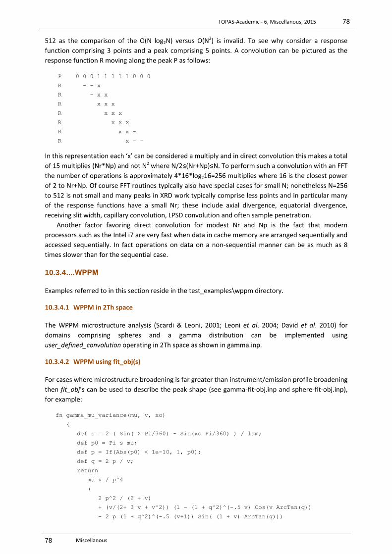
TOPAS-Academic - 6, Miscellanous, 2015 78
78 Miscellanous
512 as the comparison of the O(N log2N) versus O(N2) is invalid. To see why consider a response
function comprising 3 points and a peak comprising 5 points. A convolution can be pictured as the
response function R moving along the peak P as follows:
P 0 0 0 1 1 1 1 1 0 0 0
R - - x
R - x x
R x x x
R x x x
R x x x
R x x -
R x - -
In this representation each ‘x’ can be considered a multiply and in direct convolution this makes a total
of 15 multiplies (Nr*Np) and not N2 where N/2≤(Nr+Np)≤N. To perform such a convolution with an FFT
the number of operations is approximately 4*16*log216=256 multiplies where 16 is the closest power
of 2 to Nr+Np. Of course FFT routines typically also have special cases for small N; nonetheless N=256
to 512 is not small and many peaks in XRD work typically comprise less points and in particular many
of the response functions have a small Nr; these include axial divergence, equatorial divergence,
receiving slit width, capillary convolution, LPSD convolution and often sample penetration.
Another factor favoring direct convolution for modest Nr and Np is the fact that modern
processors such as the Intel i7 are very fast when data in cache memory are arranged sequentially and
accessed sequentially. In fact operations on data on a non-sequential manner can be as much as 8
times slower than for the sequential case.
10.3.4 ....WPPM
Examples referred to in this section reside in the test_examples\wppm directory.
10.3.4.1 WPPM in 2Th space
The WPPM microstructure analysis (Scardi & Leoni, 2001; Leoni et al. 2004; David et al. 2010) for
domains comprising spheres and a gamma distribution can be implemented using
user_defined_convolution operating in 2Th space as shown in gamma.inp.
10.3.4.2 WPPM using fit_obj(s)
For cases where microstructure broadening is far greater than instrument/emission profile broadening
then fit_obj’s can be used to describe the peak shape (see gamma-fit-obj.inp and sphere-fit-obj.inp),
for example:
fn gamma_mu_variance(mu, v, xo)
{
def s = 2 ( Sin( X Pi/360) - Sin(xo Pi/360) ) / lam;
def p0 = Pi s mu;
def p = If(Abs(p0) < 1e-10, 1, p0);
def q = 2 p / v;
return
mu v / p^4
(
2 p^2 / (2 + v)
+ (v/(2+ 3 v + v^2)) (1 - (1 + q^2)^(-.5 v) Cos(v ArcTan(q))
- 2 p (1 + q^2)^(-.5 (v+1)) Sin( (1 + v) ArcTan(q)))

TOPAS-Academic - 6, Miscellanous, 2015 79
79 Miscellanous
);
}
Example super-lorentzian.inp is useful for asking the question; can spheres with a gamma distribution
describe a 1/(1+x^2)^m type function?
Example compare-1.inp is useful for asking the question; can a Voigt fit to a particular case of
spheres with a gamma distribution?
10.3.4.3 WPPM using WPPM_ft_conv
WPPM_ft_conv describes a FT in s space and performs a convolution on phase peaks that have been
interpolated to s space, for example:
WPPM_ft_conv = 1 - 1.5 WPPM_L / D + 0.5 (WPPM_L / D)^3;
WPPM_L_max = D;
WPPM_th2_range = 25 .1 Rad Lam / (D Cos(Th));
WPPM_correct_Is
The result is then interpolated back to 2Th space. Interpolations are scaled such that I(s)ds =I(θ)dθ
when WPPM_correct_Is is defined; the effects of this scaling is typically small at low angles and
becomes noticeable at very high angles reaching a maximum at 180 degrees 2Th where the derivative
of Cos(Th) is at a maximum.
When multiple WPPM_ft_conv(s) are defined then the program will internally use the convolution
theorem.
WPPL_L is a reserved parameter name that returns the transform parameter.
WPPM_L_max defines the maximum WPPL_L.
Get(ft_0) and FT_Break can both be used in WPPM_ft_conv in a manner similar to ft_conv.
The tails of WPPM peaks extend for almost the whole diffraction pattern; they can be shortened using
WPPM_th2_range; in the above example this range has been written in terms of the fwhm as defined
in the Scherrer equation.
WPPM_ft_conv can be a function of the following reserved parameter names:
H, K, L, M, Th, Xo, D_spacing, WPPM_L and spherical_harmonics_hkl
Example s-sphere-1.inp uses WPPM_ft_conv to fit to a synthesized WPPM generated peak with
identical results.
The following macros (written by Matteo Lenoi), as defined in TOPAS.INC, describes a log normal
distribution:
WPPM_Cube_Ln_Normal
WPPM_Sphere_Ln_Normal
WPPM_Octahedron_Ln_Normal
Where for example WPPM_Octahedron_Ln_Normal is as follows:
macro WPPM_Octahedron_Ln_Normal(muc, muv, sigc, sigv)
{
#m_argu muc
#m_argu sigc
If_Prm_Eqn_Rpt(muc, muv, min .1 max = Min(2 Val + .3, 100);)

TOPAS-Academic - 6, Miscellanous, 2015 80
80 Miscellanous
If_Prm_Eqn_Rpt(sigc, sigv, min .01 max = Min(2 Val + .01, 3);)
WPPM_ft_conv =
{
def cga = Constant(Cos(Get(ga) Pi/180));
def sga = Constant(Sin(Get(ga) Pi/180));
def cal = Constant(Cos(Get(al) Pi/180));
def cbe = Constant(Cos(Get(be) Pi/180));
def aa = Constant(Get(a));
def bb = Constant(Get(b));
def cc = Constant(Get(c));
def cv = Constant(Get(cell_volume));
def wA = H / aa;
def wB = (-H cga / aa + K / bb) / sga;
def wC = ( (H bb cc (cal cga - cbe) + K aa cc (cbe cga - cal)) / sga
+ L aa bb sga) / cv;
def A = D_spacing Max(wA, wB, wC);
def B = D_spacing Max(Min(wA, wB),Min(wA, wC),Min(wB, wC));
def C = D_spacing Min(wA, wB, wC);
def H0 = 1;
def H1 = If (A>=B+C,-3 A/Sqrt(2),- 3 (A + B + C)/Sqrt(8));
def H2 = If (A>=B+C, 3 (A A - B B - C C)/2,-3(A A+(B-C)^2 - 2 A
(B+C))/4);
def H3 = If (A>=B+C, (-A^3 + 3 A (B B+C C) + 2(B^3 + C^3))/(2
Sqrt(2)),(A^3 + B^3 + C^3-3 A B C)/Sqrt(2));
def Kc = (A + B + C)/Sqrt(2);
def u = CeV(muc, muv);
def sig = CeV(sigc, sigv);
fn M(n) = Exp(Min(n u + 0.5 n^2 sig, 600));
fn wppm_Ln(kc) = Get(WPPM_Ln_k) + Ln(kc Get(WPPM_dL));
fn q(Hn, n) {
return
Hn
Erfc_Approx( ( wppm_Ln(Kc) - u - (3-n) sig^2) / (sig Sqrt(2)))
WPPM_L^n
M(3-n);
}
return q(H0, 0) + q(H1, 1) + q(H2, 2) + q(H3, 3);
}
WPPM_break_on_small = 1e-7;
WPPM_L_max 1000
WPPM_th2_range = 30;
}
Example cube-ln-normal-1.inp can be used to test these macros. Lattice parameters appearing within
the macros are made constant using Constant; these convolutions are therefore made independent of
lattice parameter changes and hence separate convolutions are not initiated whilst calculating lattice
parameter derivatives.
WPPM_Ln_k is a reserved parameter name that returns Ln of an integer and is used to calculate
Ln(Kc WPPM_L) in a fast manner.
The example ln-normal-1.inp can be used for visualizing a Ln normal distribution. It uses the
Ln_Normal_x_at_CD function to determine the limit of the distribution.
TOPAS-Academic - 6, Miscellanous, 2015 81
81 Miscellanous
10.3.5 ....Microstructure convolutions
The Double-Voigt approach (e.g. Balzar, 1999) is supported for modeling microstructure effects.
Crystallite size and strain comprise Lorentzian and Gaussian component convolutions varying in 2 as a
function of 1/cos() and tan() respectively.
10.3.5.1 Preliminary equations
The following preliminary equations are based on the unit area Gaussian, GUA(x), and Lorentzian, LUA(x),
and pseudo-Voigt PVUA(x) functions as given in Table 5-2.
Height of GUA(x) and LUA(x) respectively
GUAH = GUA(x=0) = g1 / fwhm
LUAH = LUA(x=0) = l1 / fwhm
Gaussian and Lorentzian respectively with area A
G(x) = A GUA(x)
L(x) = A LUA(x)
Height of G(x) and L(x) respectively
GH = A GUA
LH = A LUAH
Integral breadth of Gaussian and Lorentzian respectively
G = A / GH = 1 / GUAH = fwhm / g1
L = A / LH = 1 / LUAH = fwhm / l1
Unit area Pseudo Voigt, PVUA
PVUAH = LUAH + (1-) GUAH
PV = 1 / PVUAH
A Voigt is the result of a Gaussian convoluted by a Lorentzian
V = G(fwhmG) L(fwhmL)
where "" denotes convolution and fwhmG and fwhmL are the FWHM of the Gaussian and Lorentzian
components.
A Voigt can be approximated using a Pseudo Voigt. This is done numerically where
V(x) = G(fwhmG) L(fwhmL) = PVUA(x, fwhmPV)
By changing units to s (Å-1)
s = 1/d = 2 sin() /
and differentiating and approximating ds/d = s / we get
s = (2 cos() / )
thus,
fwhm(s) = fwhm(2) cos() /

TOPAS-Academic - 6, Miscellanous, 2015 82
82 Miscellanous
IB(s) = IB(2) cos() /
10.3.5.2 Crystallite size and strain
Crystallite Size
For crystallite size the Gaussian and Lorentzian component convolutions are:
fwhm(2) of Gaussian = (180/) / (cos() CS_G)
fwhm(2) of Lorentzian= (180/) / (cos() CS_L)
(2) of Gaussian = (180/) / (cos() CS_G g1)
(2) of Lorentzian = (180/) / (cos() CS_L l1)
or, according to Balzar (1999), in terms of s, GS and CS
fwhm(s) of Gaussian = (180/) / CS_G
fwhm(s) of Lorentzian = (180/) / CS_L
GS(s) =(s) of Gaussian = (180/) / (CS_G g1)
CS(s) =(s) of Lorentzian = (180/) / (CS_L l1)
The macros CS_L and CS_G are used for calculating the CS_L and CS_G parameters respectively.
Determination of the volume weighted mean column height LVol, LVol-IB and LVol-FWHM is as
follows:
LVol-IB = k / Voigt_Integral_Breadth_GL (1/CS_G, 1/CS_L)
LVol-FWHM = k / Voigt_FWHM(1/CS_G, 1/CS_L)
The macro LVol_FWHM_CS_G_L is used for calculating LVol-IB and LVol-FWHM.
Strain
Strain_G and Strain_L parameters corresponds to the fwhm(2) of a Gaussian and a Lorentzian that is
convoluted into the peak, or,
fwhm(2) of Gaussian = Strain_G tan()
fwhm(2) of Lorentzian= Strain_L tan()
(2) of Gaussian = Strain_G tan() / g1
(2) of Lorentzian = Strain_L tan() / l1
or, according to Balzar (1999), in terms of s, CD and GD
fwhm(s) of Gaussian = Strain_G sin() / = Strain_G s / 2
fwhm(s) of Lorentzian = Strain_L sin() / = Strain_L s / 2
GD(s)/s0 s = (s) of Gaussian = (Strain_G / g1) s / 2
CD(s)/s0 s = (s) of Lorentzian = (Strain_L / l1) s / 2
The macros Strain_L and Strain_G are used for calculating the Strain_L and Strain_G parameters
respectively.
From these equations we get:
GD(s) = s0 Strain_G / (2 g1)
CD(s) = s0 Strain_L / (2 l1)
TOPAS-Academic - 6, Miscellanous, 2015 83
83 Miscellanous
According to Balzar (1999), equation (34):
e = D(2) / (4 tan())
where D(2) is the fwhm of a Voigt comprising a Gaussian with a fwhm = Strain_G Tan() and a
Lorentzian with a fwhm = Strain_L Tan().
The value for e0 is given by:
4 e0 Tan() = FWHM of the Voigt from Strain_L and Strain_G
= Voigt_FWHM(Strain_L, Strain_G) Tan()
or,
e0 = Voigt_FWHM(Strain_L, Strain_G) ( / 360) / 4
The macro e0_from_Strain calculates e0 using the equation function Voigt_FWHM_GL.
10.4 . Loading of INP files
10.4.1 ....if {} else if {} else {}
An ‘if’ construct operational on the loading of INP files, see test_examples\zro2.inp. Loading operates
on the pre-processed INP file; syntax is as follows:
if expression {
} else if expression {
} else expression {
}
expression can be any valid TOPAS equation without the semicolon; in addition expression can contain
the functions Prm_There(prm_name) and Obj_There(obj_name). The following is equivalent to a /* */
block comment:
if 0 {
...
}
A more complex construct could look something like the following:
xdd
local aaa 1
str...
local aaa 2
str...
local aaa 3
hkl_Is
if Prm_There(aaa) {
Out(aaa, "\nThis is the aaa at the xdd level %-1.6f")
if aaa == 2 {
Out_String("\nThis wont be written to file as aaa at the xdd level
is 1")
}
} else if Obj_There(hkl_Is) {
Out_String("\nYes this is a hkl_Is phase")
} else {
Out_String("\naaa is not there and this is not a hkl_Is phase")

TOPAS-Academic - 6, Miscellanous, 2015 84
84 Miscellanous
}
for xdds {
if And(Obj_There(neutron), Obj_There(pk_xo)) {
' Neutron TOF
}
}
10.5 . Functions – fn, def, return, noinline
Functions can be defined using the ‘fn’ keyword; here’s an example of a recursive function:
fn factorial(x) { return If(x == 1, 1, x factorial(x-1)); }
prm = factorial(5); : 120
There’s also the simple form where the ‘return’ statement is implied:
fn factorial(x) = If(x == 1, 1, x factorial(x-1));
The equation part of ‘prm’ objects can have a function body (see the macro Robust_Refinement in
TOPAS.INC), for example
prm = { def a = 2; return a; }
Most importantly functions can reference parameters defined with the ‘prm’ keyword; this simplifies
the writing of ‘prm’ equations and additionally memory usage can be greatly reduced when the
‘noinline’ keyword is used. Equations called ‘def’ objects can be used and defined within non-simple
functions. Here’s an example:
fn gauss(a, x, f, g) {
def a1 = 2 Sqrt(Ln(2) / Pi) / f;
def a2 = 4 Ln(2);
def a3 = (x / f);
return a1 Exp(-a2 a3^2);
}
A ‘def’ object must be defined prior to its use. They can be assigned to other ‘def’ objects but not to
objects of ‘prm’ type. In other words ‘prm’ objects are write-protected within functions. The
arguments to functions can be ‘def’ or ‘prm’ objects. c-style braces can be used to scope variables; the
following will throw an exception due to the attempted use of an uninitialized ‘def’ object:
fn foo(x) { def a; { def a = x; } return a; }
prm = foo(3); : 0 ‘ Exception thrown
The following will not throw an exception as the simplification routines will recognize the ‘0’:
fn a(x) = x undefined_name 0; prm = a(3); : 0
Functions can be nested; for example:
fn foo() {
def a, b;
a = 3; b = 2;
fn nested(x, y) { return Sqrt(x^2 + y^2); }
return nested(a, b);
}
prm = foo(); : 3.60555

TOPAS-Academic - 6, Miscellanous, 2015 85
85 Miscellanous
‘def’ and ‘prm’ objects have scope and their scope determine the actual object used.
Here def ‘a’ is returned:
fn a(a) { def a = 2; return a; } prm = a(1) : 2
Here prm ‘a’ is returned:
prm a = 2; fn a() = a; prm = a(); : 2
Here the argument ‘a’ is returned:
prm a = 2; fn a(a) = a; prm = a(3); : 3
Function specifics
fn's are a kernel operation and not a pre-processor operation.
fn's must be defined prior to their use.
fn arguments are optional but parentheses must be used in both the function definition and its
use.
a fn cannot be defined with a name of a previously defined fn name.
fn's are inlined by default.
Non-nested fn’s can be prevented from being inlined with the ‘noinline’ prefix.
nested functions cannot be prefixed with ‘noinline’
Use of noinline can often be slower than not using noinline as a stack mechanism is used for the fn
arguments as well as the global simplification routines cannot simplify what’s inside a noinlined
function. Functions are therefore ‘inlined’ (the word ‘expand’ is sometimes used) by default. A macro
can be considered an inlined function and there’s no difference in the how the following is finally
processed:
fn my_max(a, b, c) = Max(a, b, c);
macro & my_max(& a, & b, & c) { Max(a, b, c) }
The macro by definition is inlined in the pre-processed INP file. In the case of ‘fn’ the program will
inline ‘my_max’. Prefixing fn with ‘noinline’ prevents inlining, for example:
noinline fn gauss(x, f)=(2 Sqrt(Ln(2)/Pi)/f) Exp(-4 Ln(2)((X-x)/f)^2);
Its best to inline small functions as it gives the simplification routines a chance to simplify what’s inside
the function in regards to its surroundings. Consider the following:
noinline fn a(b, c) = b^2 + c^2;
prm p1 1
prm !p2 1
prm p3 1
prm !p4 1
prm p5 = a(p1, p2) + a(p3, p4); : 0
Without inlining the simplification routines won’t see that p2 and p4 are constants inside the ‘a’
function and hence no simplification is performed; the ‘a’ function will be called twice and the stack
used twice. Note, stack here refers to the computer algebra stack. With inlining p5 after simplification
reduces to:
prm p5 = p1^2 + p3^2 + 2; : 0

TOPAS-Academic - 6, Miscellanous, 2015 86
86 Miscellanous
In the case of large functions then not inlining may increase performance as the signalling of equation
nodes for recalculation will be reduced. Inlined functions have scope allowing the use of the Get()
function, for example:
fn lat(h, k, l) = h Get(a) + k Get(b) + l Get(c);
str..
lor_fwhm = lat(H, K, L) - lat(-H, -K, -L);
10.5.1 ....Subject independent single crystal refinement
The \functions\alvo4-fn.inp example performs a single crystal refinement using the computer algebra
aspects of the program. No x-ray or subject dependent keywords have been used; instead only six
keywords are utilized:
fn, noinline, def, return, prm, restraint
The speed of alvo4-fn.inp is 7.4 times slower than the comparable subject dependent keyword
equivalent of alvo4-normal.inp. Much of the difference in speed is in the calculation of the Cosines
necessary for the structure factors. Importantly convergence and the behaviour of the parameters are
similar. The placement of noinline is important. Also used is the out_refinement_stats keyword which
outputs the following:
First pass equation statistics excluding attribute equations
Number of equations : 534
Number of nodes : 99751
Number of nodes if expanded : 12070283
Number of penalties/restraints: 532
Number of independent penalty/restraints parameters: 58
Number of penalties/restraints: 532
Number of independent penalty/restraints parameters: 58
Time 0.13
Second pass equation statistics excluding attribute equations
Before/After equation simplification
Number of equations : 549 553
Number of nodes : 99766 8354
Number of nodes if expanded : 12070298 228183
Number of objects taking part in refinement: 73
Number of dependent parameters with derivatives wrt to Ycalc: 15
The alvo4-fn.inp demonstrates the ease at which an entire single crystal refinement can be performed;
it should allow for user defined temperature factors etc…
10.5.2 ....Computer algebra and out_refinement_stats
The computer algebra system CAS in version 5 (Coelho et al., 2011) is around 2 to 4 times faster than
version 4; compare with running ROSENBROCK-10.INP or PVS.INP. The CAS has been reworked and it
now operates on a global level where equations are simplified across all objects. The
out_refinement_stats keywords, for SERINE_I_EVANS_N_TA_BANG_ROT.INP for example, outputs the
following equation statistics:
Second pass equation statistics excluding attribute equations
TOPAS-Academic - 6, Miscellanous, 2015 87
87 Miscellanous
Before/After equation simplification
Number of equations : 2707 3085
Number of nodes : 22941 16671
Number of nodes if expanded : 1706390373 1070170132
Number of objects taking part in refinement: 2595
Number of dependent parameters with derivatives wrt to Ycalc: 2319
10.6 . CIF
The following macros and Get’s can be used to output data in CIF format:
Out_CIF_STR(file)
Out_CIF_ADPs(file)
Out_CIF_STR(file, with_id)
Out_CIF_Bonds_Angles(file)
Get(number_of_parameters)
Get(refine_ls_shift_on_su_max)
Get(weighting)
Xi = a reserved parameter name
_refine_ls_shift/su_max can be accessed using Get(refine_ls_shift_on_su_max) when do_errors is
defined and when continue_after_convergence is NOT defined. A message similar to the following is
displayed on calculation:
refine_ls_shift_on_su_max 0.409610469 corresponds to parameter m501b939c_3 of
object prm_10
Get(weighting) and Xi can be used as follows:
xdd_out file append load out_record out_fmt out_eqn {
" %9.0f" = Xi;
" %11.5f" = X;
" %11.5f" = Ycalc;
" %11.5f" = Yobs;
" %11.5f\n" = Get(weighting);
}
Get(weighting) returns the following masked with excluded regions:
1 / Max(1, Yobs), if SigmaYobs does not exist
1 / SigmaYobs^2, if SigmaYobs does exist
If weighting is a function of YCalc etc... then it returns the last weighting calculated depending on
recal_weighting_on_iter.
10.7 . Large refinements with tens of 1000s of parameters
Refinements comprising many parameters and data points can be both slow and memory intensive.
Computation speed is hindered by the A matrix dot products of Eq. (4-4). In the case of dense
matrices, memory usage in forming the full A matix can be prohibitive. The following keywords can be
used to overcome these problems:
conserve_memory
bootstrap_errors 100

TOPAS-Academic - 6, Miscellanous, 2015 88
88 Miscellanous
approximate_A
A_matrix_memory_allowed_in_Mbytes 100
A_matrix_elements_tollerance 0.00001
The approximate_A keyword avoids the calculation of the A matrix dot products. Typically more
refinement iterations are required for convergence but in most large problems the time to
convergence is greatly decreased (see for example AE14-APPROX-A.INP). Furthermore memory usage
of the A matrix can be limited using A_matrix_memory_allowed_in_Mbytes; this produces a sparse
matrix, dependening on alloted memory, by removing small Aij values.
Typically the calculation of the covariance matrix is impractical and hence errors can instead be
determined using the bootstrap method.
10.8 .. Laue refinement
Single crystal Laue diffraction data can be refined; data files have the extension *.hkl-lam; see
directory test_examples\laue. Laue_Lam is a reserved parameter name that can be used in hkl type
equations; it returns the reflection dependent wavelength. The merging of equivalent reflections and
Friedel_pairs are not allowed with Laue refinement; the following keywords are internally defined
with Laue refinement:
dont_merge_equivalent_reflections
dont_merge_Friedel_pairs
and the following messages reported:
Equivalent reflections not merged
Friedel pairs not merged
10.9 .. Learnt Shapes for Background or Otherwise
The keywords user_y and fo_transform_X provides a means to use learnt shapes as a background
function. The test example USER_Y.INP produces the following fit to Quartz using a learnt Pseudo-
Voigt.
Example usage:
user_y NAME { #include SOME_FILE }
user_y NAME SOME_FILE
fit_obj = NAME;
fo_transform_X = (X - x) / s;
69.56968.56867.56766.5
16,000
14,000
12,000
10,000
8,000
6,000
4,000
2,000
0
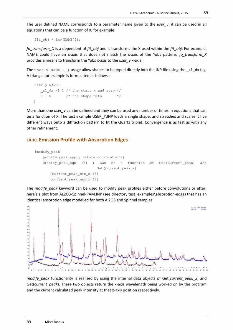
TOPAS-Academic - 6, Miscellanous, 2015 89
89 Miscellanous
The user defined NAME corresponds to a parameter name given to the user_y; it can be used in all
equations that can be a function of X, for example:
fit_obj = Exp(NAME^2);
fo_transform_X is a dependent of fit_obj and it transforms the X used within the fit_obj. For example,
NAME could have an x-axis that does not match the x-axis of the Yobs pattern; fo_transform_X
provides a means to transform the Yobs x-axis to the user_y x-axis.
The user_y NAME {…} usage allow shapes to be typed directly into the INP file using the _x1_dx tag.
A triangle for example is formulated as follows :
user_y NAME {
_x1_dx -1 1 /* the start x and step */
0 1 0 /* the shape data */
}
More than one user_y can be defined and they can be used any number of times in equations that can
be a function of X. The test example USER_Y.INP loads a single shape, and stretches and scales it five
different ways onto a diffraction pattern to fit the Quartz triplet. Convergence is as fast as with any
other refinement.
10.10 . Emission Profile with Absorption Edges
[modify_peak]
[modify_peak_apply_before_convolutions]
[modify_peak_eqn !E] : Can be a function of Get(current_peak) and
Get(current_peak_x)
[current_peak_min_x !E]
[current_peak_max_x !E]
The modify_peak keyword can be used to modify peak profiles either before convolutions or after;
here’s a plot from AL2O3-Spinnel-PAM.INP (see directory test_examples\absorption-edge) that has an
identical absorption edge modelled for both Al2O3 and Spinnel samples:
modify_peak functionality is realized by using the internal data objects of Get(current_peak_x) and
Get(current_peak). These two objects return the x-axis wavelength being worked on by the program
and the current calculated peak intensity at that x-axis position respectively.

TOPAS-Academic - 6, Miscellanous, 2015 90
90 Miscellanous
10.11 . scale_phase_X keyword
The scale_phase_X keyword scales Ycalc point by point. It can be used to define say alternate Lorentz
Polarization factors. Some main points:
Can be a function of X
Multiple definitions are allowed and each is applied to the pattern.
Can occur at the xdd or phase level.
Here’s an example:
xdd…
scale_phase_X…
str…
scale_phase_X…
hkl_Is…
scale_phase_X…
The first str is multiplied by the first and second scale_phase_X; the hkl_Is phase is multiplied by the
first and third scale_phase_X.
10.12 . Refining on f0, f’ and f’’
[f0_f1_f11_atom]…
[f0 E] [f1 E] [f11 E]
Example usage is as follows:
report_on_str
load f0_f1_f11_atom f1 f11 {
Ba @ -0.160127754 2.3954287
Ge 0.184162081 1.86162161
}
High correlations exist between f1 and f11, scale and beq parameters.
The f0_f1_f11_atom keyword can be used at the str, xdd and global levels. f’ or f’’ can be defined
and refined independently. Defaults are used when either f’ or f‘’ are not defined. The XRAY-
POWDER.INP and TOF.INP in the directory test_examples\f0-f1-f11\ demonstrates the use of f0, f1 and
f11.
The f0 parameter can be a function of the reserved parameter D_spacing; for example:
prm a1 25 min -50 max 50
load f0_f1_f11_atom f0 f11 {
Pb+2
= a1 Exp(1.058874 (-0.25) / D_spacing^2) +
16.496822 Exp(0.106305 (-0.25) / D_spacing^2) +
19.984501 Exp(6.708123 (-0.25) / D_spacing^2) +
6.813923 Exp(24.395554 (-0.25) / D_spacing^2) +
5.233910 Exp(1.058874 (-0.25) / D_spacing^2) +
4.065623; ' this is f0 for Pb
@ 5 ' this is f11 for Pb
}
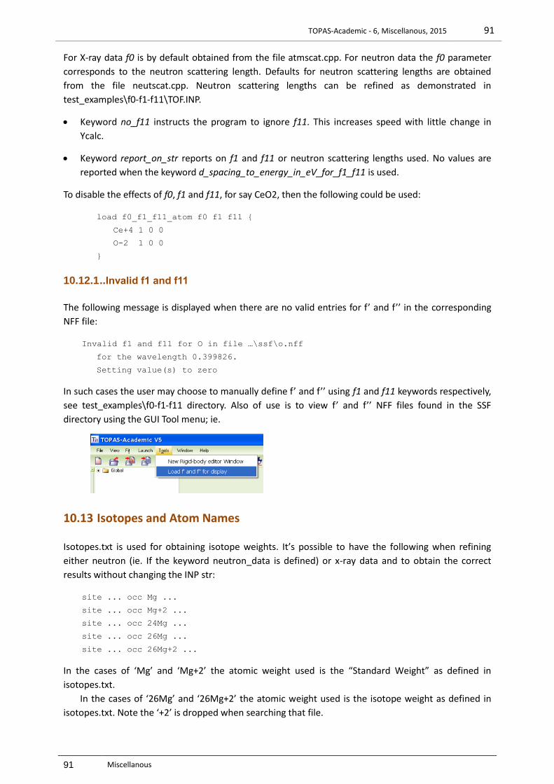
TOPAS-Academic - 6, Miscellanous, 2015 91
91 Miscellanous
For X-ray data f0 is by default obtained from the file atmscat.cpp. For neutron data the f0 parameter
corresponds to the neutron scattering length. Defaults for neutron scattering lengths are obtained
from the file neutscat.cpp. Neutron scattering lengths can be refined as demonstrated in
test_examples\f0-f1-f11\TOF.INP.
Keyword no_f11 instructs the program to ignore f11. This increases speed with little change in
Ycalc.
Keyword report_on_str reports on f1 and f11 or neutron scattering lengths used. No values are
reported when the keyword d_spacing_to_energy_in_eV_for_f1_f11 is used.
To disable the effects of f0, f1 and f11, for say CeO2, then the following could be used:
load f0_f1_f11_atom f0 f1 f11 {
Ce+4 1 0 0
O-2 1 0 0
}
10.12.1 ..Invalid f1 and f11
The following message is displayed when there are no valid entries for f’ and f’’ in the corresponding
NFF file:
Invalid f1 and f11 for O in file …\ssf\o.nff
for the wavelength 0.399826.
Setting value(s) to zero
In such cases the user may choose to manually define f’ and f’’ using f1 and f11 keywords respectively,
see test_examples\f0-f1-f11 directory. Also of use is to view f’ and f’’ NFF files found in the SSF
directory using the GUI Tool menu; ie.
10.13 Isotopes and Atom Names
Isotopes.txt is used for obtaining isotope weights. It’s possible to have the following when refining
either neutron (ie. If the keyword neutron_data is defined) or x-ray data and to obtain the correct
results without changing the INP str:
site ... occ Mg ...
site ... occ Mg+2 ...
site ... occ 24Mg ...
site ... occ 26Mg ...
site ... occ 26Mg+2 ...
In the cases of ‘Mg’ and ‘Mg+2’ the atomic weight used is the “Standard Weight” as defined in
isotopes.txt.
In the cases of ‘26Mg’ and ‘26Mg+2’ the atomic weight used is the isotope weight as defined in
isotopes.txt. Note the ‘+2’ is dropped when searching that file.
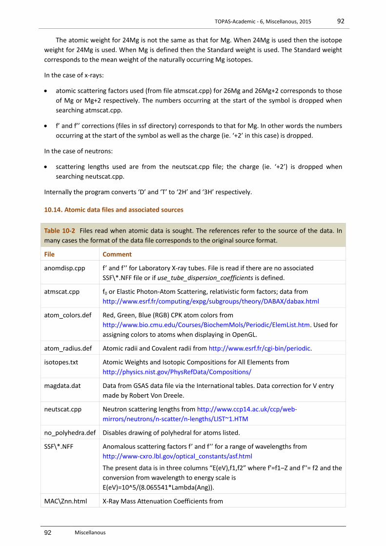
TOPAS-Academic - 6, Miscellanous, 2015 92
92 Miscellanous
The atomic weight for 24Mg is not the same as that for Mg. When 24Mg is used then the isotope
weight for 24Mg is used. When Mg is defined then the Standard weight is used. The Standard weight
corresponds to the mean weight of the naturally occurring Mg isotopes.
In the case of x-rays:
atomic scattering factors used (from file atmscat.cpp) for 26Mg and 26Mg+2 corresponds to those
of Mg or Mg+2 respectively. The numbers occurring at the start of the symbol is dropped when
searching atmscat.cpp.
f’ and f’’ corrections (files in ssf directory) corresponds to that for Mg. In other words the numbers
occurring at the start of the symbol as well as the charge (ie. ‘+2’ in this case) is dropped.
In the case of neutrons:
scattering lengths used are from the neutscat.cpp file; the charge (ie. ‘+2’) is dropped when
searching neutscat.cpp.
Internally the program converts ‘D’ and ‘T’ to ‘2H’ and ‘3H’ respectively.
10.14 . Atomic data files and associated sources
Table 10-2 Files read when atomic data is sought. The references refer to the source of the data. In
many cases the format of the data file corresponds to the original source format.
File Comment
anomdisp.cpp f’ and f’’ for Laboratory X-ray tubes. File is read if there are no associated
SSF\*.NFF file or if use_tube_dispersion_coefficients is defined.
atmscat.cpp f0 or Elastic Photon-Atom Scattering, relativistic form factors; data from
http://www.esrf.fr/computing/expg/subgroups/theory/DABAX/dabax.html
atom_colors.def Red, Green, Blue (RGB) CPK atom colors from
http://www.bio.cmu.edu/Courses/BiochemMols/Periodic/ElemList.htm. Used for
assigning colors to atoms when displaying in OpenGL.
atom_radius.def Atomic radii and Covalent radii from http://www.esrf.fr/cgi-bin/periodic.
isotopes.txt Atomic Weights and Isotopic Compositions for All Elements from
http://physics.nist.gov/PhysRefData/Compositions/
magdata.dat Data from GSAS data file via the International tables. Data correction for V entry
made by Robert Von Dreele.
neutscat.cpp Neutron scattering lengths from http://www.ccp14.ac.uk/ccp/web-
mirrors/neutrons/n-scatter/n-lengths/LIST~1.HTM
no_polyhedra.def Disables drawing of polyhedral for atoms listed.
SSF\*.NFF Anomalous scattering factors f’ and f’’ for a range of wavelengths from
http://www-cxro.lbl.gov/optical_constants/asf.html
The present data is in three columns “E(eV),f1,f2” where f'=f1–Z and f''= f2 and the
conversion from wavelength to energy scale is
E(eV)=10^5/(8.065541*Lambda(Ang)).
MAC\Znn.html X-Ray Mass Attenuation Coefficients from
TOPAS-Academic - 6, Miscellanous, 2015 93
93 Miscellanous
http://www.nist.gov/pml/data/xraycoef/index.cfm
10.15 Removing Phases during a refinement
The remove_phase keyword (used by the Remove_Phase macro) allows for phase removal during
refinement. Typical use is as follows:
for strs {
Remove_Phase(0.3, 0.5)
}
Here a phase is removed if its weight percent is below 0.3% and if the error in the weight percent is
greater than 0.5 times the weight percent. The phase removal process is executed at the end of a
Cycle. Text similar to the following is displayed on removal of a phase:
*** Deleting phase: Corundum ***
*** Deleting phase: Zincite ***
... etc...
Refinement is terminated when no phase is removed during a Cycle.
10.16 Numerical Lorentzian and Gaussian Convolutions
For fundamental and pseudo-Voigt peak types, Lorentzian and Gaussian convolutions are performed
analytically during the calculation of the emission profile Voigt. Therefore when lor_fwhm and
gauss_fwhm are defined within push_peak and add_pop_1st_2nd_peak keywords they are still
calculated at the emission profile level.
10.17 Space groups, hkls and symmetry operators
[space_group $symbol] is used to define the space group where $symbol can be any space group
symbol (case insensitive) occurring in the file SGCOM5.CPP, it can also be a space group number; here
are some examples:
space_group "I a -3"
space_group ia-3
space_group P_63_M_C
space_group I_41/A_M_D
space_group I_41/A_M_D:2 ' defines second setting of I_41/A_M_D
space_group 206
space_group 222:2 ' defines second setting of 222
Symmetry operators are generated by SGCOM6.EXE and placed into a sg\*.sg file with a name similar
to the name of the space group. Space group names containing the characters ‘/’ or ‘:’ are placed in
files with file names similar to the space group but with the characters replaced by ‘o’ and ‘q’
respectively. The reason for this is that file names containing these characters are not allowed on some
operating systems. hkl generation uses information in the *.sg file.
10.17.1 ... User defined rotational matrices
Space group generator - User defined rotational matrices can be added to the file sgrots3.cpp found in
the main TA directory.

TOPAS-Academic - 6, Miscellanous, 2015 94
94 Miscellanous
10.18 Site identifying strings
Keywords such as operate_on_points use a site identifying string; this string can contain the wild card
character ’*’ and a negation character ’!’. The wild card character ‘*’ used in “O*” means that sites with
names starting with ‘O’ are considered. In addition to using the wild card character, site names can be
written explicitly within double quotation marks. For example, consider the following segment:
str
site Pb1...
site S1 ...
site O1 ...
site O2 ...
site O31 ...
site O32 ...
site O4 ...
Table 10-3 shows some operate_on_points strings and the corresponding sites identified for this
particular example.
Table 10-3 Example operate_on_points strings and the corresponding sites identified.
operate_on_points $sites: Sites identified
* Pb1, S1, O1, O2, O31, O32, O4
Pb* Pb1
“Pb1 S*“ Pb1, S1
O* O1, O2, O31, O32, O4
“O* !O3*“ O1, O2, O4
“O* !O1 !O2“ O31, O32, O4
10.19 Occupancies and symmetry operators
Only unique positions are generated from symmetry operators. Fully occupied sites therefore require
site occupancy values of 1. A comparison of atomic positions is performed in the generation of the
unique positions with a tolerance in fractional coordinates of 10-15. It is therefore necessary to enter
fractions in the form of equations when entering fractional atomic coordinates that have recurring
values such as 0.33333..., 0.666666... etc., for example, use
x = 1/3; y = 1/3; z = 2/3;
instead of
x 0.33333 y 0.33333 z 0.66666
10.20 Pawley and Le Bail extraction
For Pawley intensity extraction (see example PAWLEY1.INP) the following input segment can be used
hkl_Is
space_group p-1
For Le Bail intensity extraction (see example LEBAIL1.INP) the following input segment can be used
hkl_Is
lebail 1
TOPAS-Academic - 6, Miscellanous, 2015 95
95 Miscellanous
space_group p-1
hkls are generated if there are no hkl_m_d_th2 and I keywords defined. After refinement, the details
for the generated hkl’s are appended after the space_group keyword. For the Pawley method, once
the hkl details are generated, parameter equations can be applied to the I parameters as usual.
10.21 Anisotropic refinement models
Keywords that can be a function of H, K, L and M, as shown in Table 2-3, allow for the refinement of
anisotropic models including preferred orientation, and peak broadening. An important consideration
when dealing with hkls in equations is whether to work with hkls or whether to work with their
multiplicities. The Multiplicities_Sum macro can be used when working with multiplicities, for
example:
prm a 0
th2_offset = Multiplicities_Sum( If(Mod(L,2)==0, a Tan(Th), 0) );
L here corresponds to the L's of the multiplicities. Note, the preferred orientation macro PO uses the
Multiplicities_Sum macro and Spherical Harmonics uses the hkls in the *.hkl file only.
A completely different viewpoint than to refine on half widths is to consider the distribution of
lattice metric parameters within a sample. Each crystallite is regarded as having its own lattice
parameters, with a multi-dimensional distribution throughout the powder sample. This can be
achieved by adding the same structure several times to the input file.
10.21.1 ..Second rank tensors
Anisotropic peak broadening using the Cagliotti relation. A qualitative account for anisotropic
broadening in profile analysis has been given by Le Bail & Jouanneaux (1997). A macro applying this
model could look like the following:
macro LeBail_Jouanneaux_1997(
uc11,uv11,uc22,uv22,
uc33,uv33,uc23,uv23,
uc13,uv13,uc12,uv12,
vc11,vv11,...)
{
prm u 0 min -1 max 2
prm v 0 min -1 max 1
prm w 0.01 min -1 max 2
prm uc11 uv11 prm uc22 uv22 prm uc33 uv33
...
u = (
H^2 A_star A_star uc11 +
...
v = (
H^2 A_star A_star vc11 +
...
w = ...
gauss_fwhm = u Tan(Th)^2 + v Tan(Th) + w;
}
According to Le Bail & Jouanneaux (1997) the following symmetry restrictions have to be considered:

TOPAS-Academic - 6, Miscellanous, 2015 96
96 Miscellanous
Cubic : 11=22=33, 12=13=23
Hexagonal
Trigonal : 11=22, 13=23
Tetragonal
Orthorhombic
Monoclinic : None
Triclinic
An analogous variation may also be applied to peak shapes, so a maximum of 36 refineable parameters
is obtained.
As the Cagliotti relation is a poor performer in describing half width dependence on 2 for X-ray
data and as the extremely high parameter number will not allow for stable and reliable refinements,
the examples outlined in sections 10.21.2 and 10.21.3 should be preferred as a base for describing
anisotropic peak broadening.
10.21.2 ..Spherical harmonics
The spherical_harmonics_hkl keyword can be applied to both peak shapes for anisotropy and
intensities for a preferred orientation correction. Preferred orientation can be described using the
PO_Spherical_Harmonics(sh, order) macro, where "sh" is the parameter name and "order" the order
of the spherical harmonics. The scale_pks keyword is used to correct peak intensities.
macro PO_Spherical_Harmonics(sh, order) {
spherical_harmonics_hkl sh
sh_order order
scale_pks = sh;
}
Example CLAY.INP uses spherical_harmonics_hkl for describing anisotropic peak broadening using the
exp_conv_const convolution as follows:
str...
spherical_harmonics_hkl sh
sh_order 8
exp_conv_const = (sh-1) Tan(Th);
10.21.3 ..Miscellaneous models using User defined equations
Anisotropic Gaussian convolution broadening as a function of L (see example CEO2HKL.INP):
str...
prm a 0.1 min 0.0001 max 5
prm b 0.1 min 0.0001 max 5
gauss_fwhm = If(L==0, a Tan(Th) + .2, b Tan(Th));
Anisotropic peak shifts as a function of L (th2_offset):
str...
prm at 0.07 min 0.0001 max 1
prm bt 0.07 min 0.0001 max 1
th2_offset = If(L==0, at Tan(Th), bt Tan(Th));
Description of anisotropic peak broadening using the March (1932) relation and str_hkl_angle:
str...
str_hkl_angle ang1 1 0 0
prm p1 1 min 0.0001 max 2

TOPAS-Academic - 6, Miscellanous, 2015 97
97 Miscellanous
prm p2 0.01 min 0.0001 max 0.1
lor_fwhm = p2 Tan(Th) Multiplicities_Sum(((p1^2 Cos(ang1)^2 +
Sin(ang1)^2 / p1)^(-1.5)));
10.22 Rigid bodies and bond length restraints
Rigid bodies comprise points in space defined using either the z_matrix or point_for_site keywords or
both simultaneously. All or some of these points can then be operated on using the rotate and
translate keywords. Rigid body operations typically comprise:
Translating a rigid body or part of a rigid body.
Rotating a rigid body or part of a rigid body around a point.
Rotating a rigid body or part of a rigid body around a line.
ua, ub, and uc of the point_for_site keyword, ta, tb and tc of the translate keyword, qa, qb and qc of
the rotate keyword and the parameters of the z_matrix keyword are all refineable parameters. This
means that parameter attributes such as min/max can be defined.
The following Web addresses further describes the use of Z-matrices:
http://www.chemistry.mcmaster.ca/help/yaehmop/bind_manual/node92.html
http://www.cchem.berkeley.edu/~mhggrp/class295/zmat.html
http://theo1.theochem.tu-muenchen.de/qcl/help/zmatrix_e.html
The directory RIGID contains rigid body examples in *.RGD files. These files can be viewed and
modified using the Rigid-Body-Editor of the GUI.
10.22.1 ..Fractional, Cartesian and Z-matrix coordinates
The most basic means of setting up a rigid body is by means of fractional or Cartesian coordinates. A
Benzene ring for example without Hydrogens can be formulated as follows:
prm a 1.3 min 1.2 max 1.4
rigid
point_for_site C1 ux = a Sqrt(3) .5; uy = a .5;
point_for_site C2 ux = a Sqrt(3) .5; uy = -a .5;
point_for_site C3 ux = -a Sqrt(3) .5; uy = a .5;
point_for_site C4 ux = -a Sqrt(3) .5; uy = -a .5;
point_for_site C5 uy = a;
point_for_site C6 uy = -a;
‘ rotate all previously defined points:
Rotate_about_axies(@ 0, @ 0, @ 0)
‘ translate all previously defined points:
Translate(@ .1, @ .2, @ .3)
The last two statements rotates and translates the rigid body as a whole and their inclusion are implied
if absent in the following examples.
A formulation of any complexity can be obtained from a) databases of existing structures and
simply using fractional or Cartesian coordinates of structure fragments or b) from sketch programs for
drawing chemical structures.

TOPAS-Academic - 6, Miscellanous, 2015 98
98 Miscellanous
A Z-matrix representation of a rigid body explicitly defines the rigid body in terms of bond lengths
and angles. A Benzene ring is typically formulated using two dummy atoms X1 and X2 as follows:
str...
site X1... occ C 0
site X2... occ C 0
rigid
load z_matrix {
X1
X2 X1 1.0
C1 X2 1.3 X1 90
C2 X2 1.3 X1 90 C1 60.0
C3 X2 1.3 X1 90 C2 60.0
C4 X2 1.3 X1 90 C3 60.0
C5 X2 1.3 X1 90 C4 60.0
C6 X2 1.3 X1 90 C5 60.0
}
Atoms with occupancies fixed to zero (dummy atoms) do not take part in structure factor calculations.
Importantly however dummy atoms can take part in penalties. The mixing of point_for_site and
z_matrix keywords is possible as follows:
rigid
point_for_site X1
load z_matrix {
X2 X1 1.0
C1 X2 1.3 X1 90
...
}
Z-matrix parameters are like any other parameter; they can be equations and parameter attributes
can be assigned. For example, the 1.3 bond distance can be refined as follows:
rigid
point_for_site X1
load z_matrix {
X2 X1 1.0
C1 X2 c1c2 1.3 min 1.2 max 1.4 X1 90
C2 X2 =c1c2; X1 90 C1 60.0
C3 X2 =c1c2; X1 90 C2 60.0
C4 X2 =c1c2; X1 90 C3 60.0
C5 X2 =c1c2; X1 90 C4 60.0
C6 X2 =c1c2; X1 90 C5 60.0
}
This ability to constrain Z-matrix parameters through the use of equations allows for great flexibility.
Example use of such equations could involve writing a particular Z-matrix bond length parameter in
terms of other bond length parameters whereby the average bond length is maintained. Or, in cases
where a bond length is expected to change as a function of a site occupancy then an equation relating
the bond length as a function of the site occupancy parameter can be formulated.

TOPAS-Academic - 6, Miscellanous, 2015 99
99 Miscellanous
10.22.2 ..Translating part of a rigid body
Once a starting rigid body model is defined, further translate and rotate statements can be included to
represent deviations from the starting model. For example, if the C1 and C2 atoms are expected to
shift by up to 0.1Å and as a unit then the following could be used:
rigid
load z_matrix {
X1
X2 X1 1.0
C1 X2 1.3 X1 90
C2 X2 1.3 X1 90 C1 60.0
C3 X2 1.3 X1 90 C2 60.0
C4 X2 1.3 X1 90 C3 60.0
C5 X2 1.3 X1 90 C4 60.0
C6 X2 1.3 X1 90 C5 60.0
}
translate
tx @ 0 min -.1 max .1
ty @ 0 min -.1 max .1
tz @ 0 min -.1 max .1
operate_on_points "C1 C2"
where the additional statements are outlined in bold. The Cartesian coordinate representation allows
an additional means of shifting the C1 and C2 atoms by refining on the ux, uy and uz coordinates
directly, or,
prm a 1.3 min 1.2 max 1.4
prm t1 0 min -.1 max .1
prm t2 0 min -.1 max .1
prm t3 0 min -.1 max .1
rigid
point_for_site C1 ux = a Sqrt(3) .5 + t1; uy = a .5 + t2; uz = t3;
point_for_site C2 ux = a Sqrt(3) .5 + t1; uy = -a .5 + t2; uz = t3;
point_for_site C3 ux = -a Sqrt(3) .5; uy = a .5;
point_for_site C4 ux = -a Sqrt(3) .5; uy = -a .5;
point_for_site C5 uy = a;
point_for_site C6 uy = -a;
10.22.3 ..Rotating part of a rigid body around a point
Many situations require the rotation of part of a rigid body around a point. An octahedra (Fig. 10-1) for
example typically rotates around the central atom with three degrees of freedom. To implement such a
rotation when the central atom is arbitrarily placed requires setting the origin at the central atom
before rotation and then resetting the origin after rotation. This is achieved using the
Translate_point_amount macro as follows:
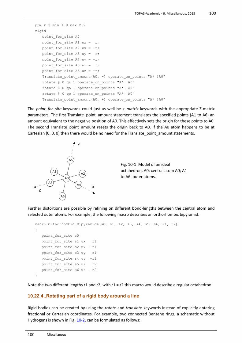
TOPAS-Academic - 6, Miscellanous, 2015 100
100 Miscellanous
prm r 2 min 1.8 max 2.2
rigid
point_for_site A0
point_for_site A1 ux = r;
point_for_site A2 ux = -r;
point_for_site A3 uy = r;
point_for_site A4 uy = -r;
point_for_site A5 uz = r;
point_for_site A6 uz = -r;
Translate_point_amount(A0, -) operate_on_points "A* !A0"
rotate @ 0 qa 1 operate_on_points "A* !A0"
rotate @ 0 qb 1 operate_on_points "A* !A0"
rotate @ 0 qc 1 operate_on_points "A* !A0"
Translate_point_amount(A0, +) operate_on_points "A* !A0"
The point_for_site keywords could just as well be z_matrix keywords with the appropriate Z-matrix
parameters. The first Translate_point_amount statement translates the specified points (A1 to A6) an
amount equivalent to the negative position of A0. This effectively sets the origin for these points to A0.
The second Translate_point_amount resets the origin back to A0. If the A0 atom happens to be at
Cartesian (0, 0, 0) then there would be no need for the Translate_point_amount statements.
Fig. 10-1 Model of an ideal
octahedron. A0: central atom A0; A1
to A6: outer atoms.
Further distortions are possible by refining on different bond-lengths between the central atom and
selected outer atoms. For example, the following macro describes an orthorhombic bipyramid:
macro Orthorhombic_Bipyramide(s0, s1, s2, s3, s4, s5, s6, r1, r2)
{
point_for_site s0
point_for_site s1 ux r1
point_for_site s2 ux –r1
point_for_site s3 uy r1
point_for_site s4 uy –r1
point_for_site s5 uz r2
point_for_site s6 uz –r2
}
Note the two different lengths r1 and r2; with r1 = r2 this macro would describe a regular octahedron.
10.22.4 ..Rotating part of a rigid body around a line
Rigid bodies can be created by using the rotate and translate keywords instead of explicitly entering
fractional or Cartesian coordinates. For example, two connected Benzene rings, a schematic without
Hydrogens is shown in Fig. 10-2, can be formulated as follows:
A3
A2 A1
A4
A5
A6
A0
Y
X Z

TOPAS-Academic - 6, Miscellanous, 2015 101
101 Miscellanous
prm r 1.3 min 1.2 max 1.4
rigid
point_for_site C1 ux = r;
load point_for_site ux rotate qz operate_on_points {
C2 =r; 60 1 C2
C3 =r; 120 1 C3
C4 =r; 180 1 C4
C5 =r; 240 1 C5
C6 =r; 300 1 C6
}
point_for_site C7 ux = r;
load point_for_site ux rotate qz operate_on_points {
C8 =r; 60 1 C8
C9 =r; 120 1 C9
C10 =r; 300 1 C10
}
translate tx = 1.5 r; ty = r Sin(60 Deg);
operate_on_points "C7 C8 C9 C10"
The points of the second ring can be rotated around the line connecting C1 to C2 with the following:
Rotate_about_points(@ 50 min -60 max 60, C1, C2, "C7 C8 C9 C10")
The min/max statements limit the rotations to 30 degrees.
C5 can be rotated around the line connecting C4 and C6 with the following:
Rotate_about_points(@ 40 min -50 max 50, C4, C6, C5)
Similar Rotate_about_points statements for each atom would allow for distortions of the Benzene
rings without changing bond distances.
Fig. 10-2. Model of two connected
Benzene rings
10.22.5 ..Benefits of using Z-matrix together with rotate and translate
Cyclopentadienyl (C5H5)- is a well defined molecular fragment which shows slight deviation from a
perfect five-fold ring (Fig. 10-3). The rigid body definition using point_for_site keywords is as follows:
prm r1 1.19
prm r2 2.24
rigid
load point_for_site ux { C1 =r1; C2 =r1; C3 =r1; C4 =r1; C5 =r1; }
load point_for_site ux { H1 =r2; H2 =r2; H3 =r2; H4 =r2; H5 =r2; }
load rotate qz operate_on_points { 72 1 C2 144 1 C3
216 1 C4 288 1 C5 }
load rotate qz operate_on_points { 72 1 H2 144 1 H3
216 1 H4 288 1 H5 }
C7
C4 C8 C2
C1 C5
C3 C9
C6 C10
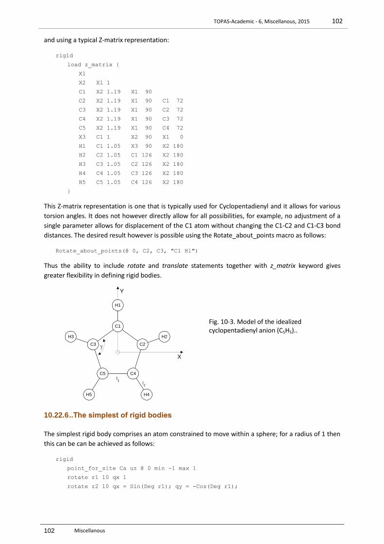
TOPAS-Academic - 6, Miscellanous, 2015 102
102 Miscellanous
and using a typical Z-matrix representation:
rigid
load z_matrix {
X1
X2 X1 1
C1 X2 1.19 X1 90
C2 X2 1.19 X1 90 C1 72
C3 X2 1.19 X1 90 C2 72
C4 X2 1.19 X1 90 C3 72
C5 X2 1.19 X1 90 C4 72
X3 C1 1 X2 90 X1 0
H1 C1 1.05 X3 90 X2 180
H2 C2 1.05 C1 126 X2 180
H3 C3 1.05 C2 126 X2 180
H4 C4 1.05 C3 126 X2 180
H5 C5 1.05 C4 126 X2 180
}
This Z-matrix representation is one that is typically used for Cyclopentadienyl and it allows for various
torsion angles. It does not however directly allow for all possibilities, for example, no adjustment of a
single parameter allows for displacement of the C1 atom without changing the C1-C2 and C1-C3 bond
distances. The desired result however is possible using the Rotate_about_points macro as follows:
Rotate_about_points(@ 0, C2, C3, "C1 H1")
Thus the ability to include rotate and translate statements together with z_matrix keyword gives
greater flexibility in defining rigid bodies.
Fig. 10-3. Model of the idealized cyclopentadienyl anion (C5H5)..
10.22.6 ..The simplest of rigid bodies
The simplest rigid body comprises an atom constrained to move within a sphere; for a radius of 1 then
this can be can be achieved as follows:
rigid
point_for_site Ca uz @ 0 min -1 max 1
rotate r1 10 qx 1
rotate r2 10 qx = Sin(Deg r1); qy = -Cos(Deg r1);
H3 H2
H4 H5
C3 C2
C4 C5 l 1
l 2
H1
C1
Y
X
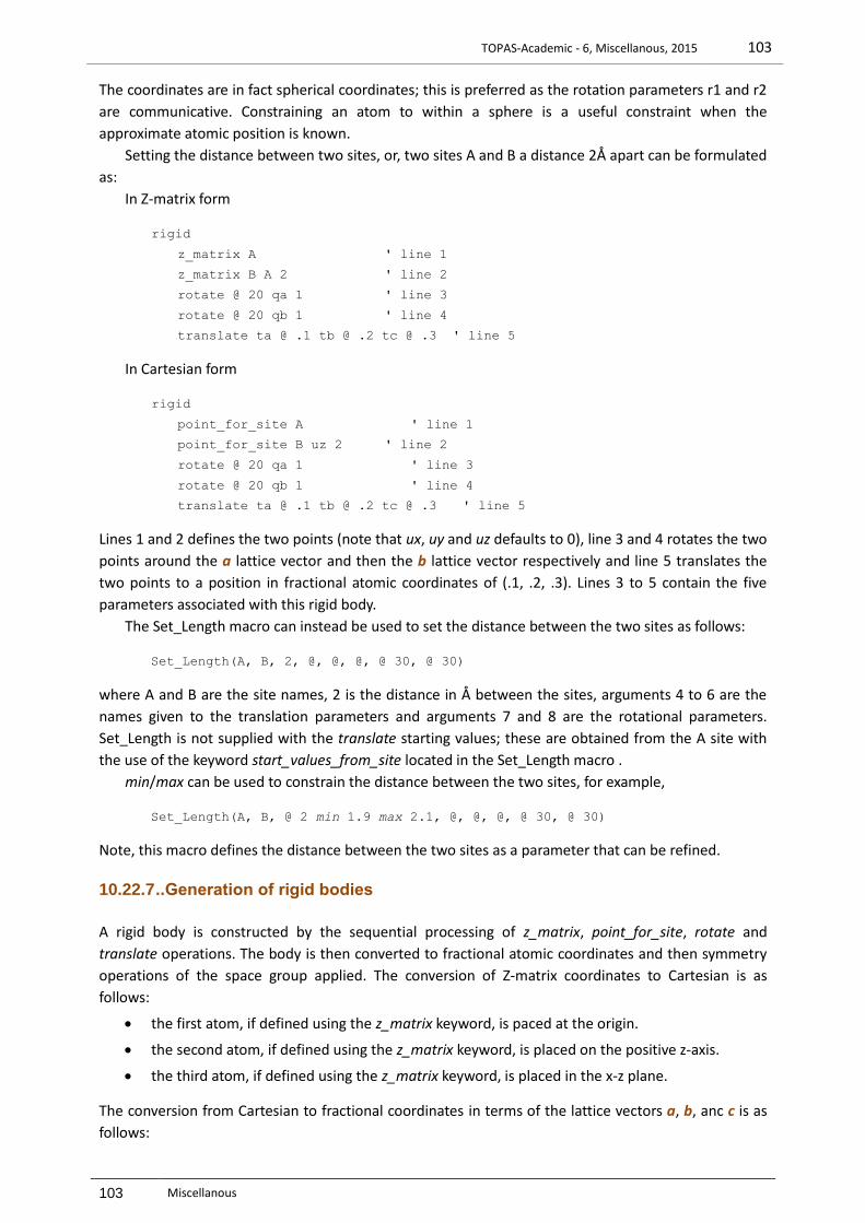
TOPAS-Academic - 6, Miscellanous, 2015 103
103 Miscellanous
The coordinates are in fact spherical coordinates; this is preferred as the rotation parameters r1 and r2
are communicative. Constraining an atom to within a sphere is a useful constraint when the
approximate atomic position is known.
Setting the distance between two sites, or, two sites A and B a distance 2Å apart can be formulated
as:
In Z-matrix form
rigid
z_matrix A ' line 1
z_matrix B A 2 ' line 2
rotate @ 20 qa 1 ' line 3
rotate @ 20 qb 1 ' line 4
translate ta @ .1 tb @ .2 tc @ .3 ' line 5
In Cartesian form
rigid
point_for_site A ' line 1
point_for_site B uz 2 ' line 2
rotate @ 20 qa 1 ' line 3
rotate @ 20 qb 1 ' line 4
translate ta @ .1 tb @ .2 tc @ .3 ' line 5
Lines 1 and 2 defines the two points (note that ux, uy and uz defaults to 0), line 3 and 4 rotates the two
points around the a lattice vector and then the b lattice vector respectively and line 5 translates the
two points to a position in fractional atomic coordinates of (.1, .2, .3). Lines 3 to 5 contain the five
parameters associated with this rigid body.
The Set_Length macro can instead be used to set the distance between the two sites as follows:
Set_Length(A, B, 2, @, @, @, @ 30, @ 30)
where A and B are the site names, 2 is the distance in Å between the sites, arguments 4 to 6 are the
names given to the translation parameters and arguments 7 and 8 are the rotational parameters.
Set_Length is not supplied with the translate starting values; these are obtained from the A site with
the use of the keyword start_values_from_site located in the Set_Length macro .
min/max can be used to constrain the distance between the two sites, for example,
Set_Length(A, B, @ 2 min 1.9 max 2.1, @, @, @, @ 30, @ 30)
Note, this macro defines the distance between the two sites as a parameter that can be refined.
10.22.7 ..Generation of rigid bodies
A rigid body is constructed by the sequential processing of z_matrix, point_for_site, rotate and
translate operations. The body is then converted to fractional atomic coordinates and then symmetry
operations of the space group applied. The conversion of Z-matrix coordinates to Cartesian is as
follows:
the first atom, if defined using the z_matrix keyword, is paced at the origin.
the second atom, if defined using the z_matrix keyword, is placed on the positive z-axis.
the third atom, if defined using the z_matrix keyword, is placed in the x-z plane.
The conversion from Cartesian to fractional coordinates in terms of the lattice vectors a, b, anc c is as
follows:
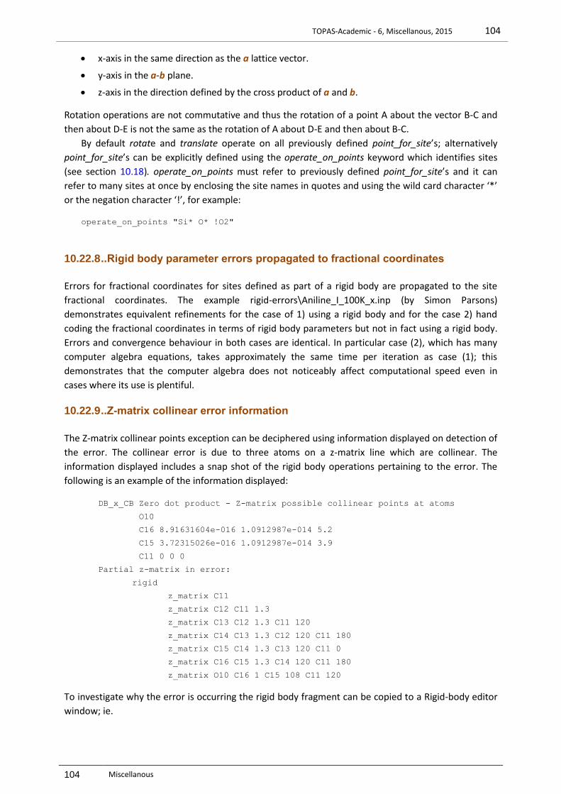
TOPAS-Academic - 6, Miscellanous, 2015 104
104 Miscellanous
x-axis in the same direction as the a lattice vector.
y-axis in the a-b plane.
z-axis in the direction defined by the cross product of a and b.
Rotation operations are not commutative and thus the rotation of a point A about the vector B-C and
then about D-E is not the same as the rotation of A about D-E and then about B-C.
By default rotate and translate operate on all previously defined point_for_site’s; alternatively
point_for_site’s can be explicitly defined using the operate_on_points keyword which identifies sites
(see section 10.18). operate_on_points must refer to previously defined point_for_site’s and it can
refer to many sites at once by enclosing the site names in quotes and using the wild card character ‘*’
or the negation character ‘!’, for example:
operate_on_points "Si* O* !O2"
10.22.8 ..Rigid body parameter errors propagated to fractional coordinates
Errors for fractional coordinates for sites defined as part of a rigid body are propagated to the site
fractional coordinates. The example rigid-errors\Aniline_I_100K_x.inp (by Simon Parsons)
demonstrates equivalent refinements for the case of 1) using a rigid body and for the case 2) hand
coding the fractional coordinates in terms of rigid body parameters but not in fact using a rigid body.
Errors and convergence behaviour in both cases are identical. In particular case (2), which has many
computer algebra equations, takes approximately the same time per iteration as case (1); this
demonstrates that the computer algebra does not noticeably affect computational speed even in
cases where its use is plentiful.
10.22.9 ..Z-matrix collinear error information
The Z-matrix collinear points exception can be deciphered using information displayed on detection of
the error. The collinear error is due to three atoms on a z-matrix line which are collinear. The
information displayed includes a snap shot of the rigid body operations pertaining to the error. The
following is an example of the information displayed:
DB_x_CB Zero dot product - Z-matrix possible collinear points at atoms
O10
C16 8.91631604e-016 1.0912987e-014 5.2
C15 3.72315026e-016 1.0912987e-014 3.9
C11 0 0 0
Partial z-matrix in error:
rigid
z_matrix C11
z_matrix C12 C11 1.3
z_matrix C13 C12 1.3 C11 120
z_matrix C14 C13 1.3 C12 120 C11 180
z_matrix C15 C14 1.3 C13 120 C11 0
z_matrix C16 C15 1.3 C14 120 C11 180
z_matrix O10 C16 1 C15 108 C11 120
To investigate why the error is occurring the rigid body fragment can be copied to a Rigid-body editor
window; ie.

TOPAS-Academic - 6, Miscellanous, 2015 105
105 Miscellanous
The O10 line is commented out as it’s the line in error. Looking at the O10 line (using the OpenGL
window) it can be seen that atoms C16, C15, C11 lie on a straight line; this is invalid as it becomes
impossible to form the dihedral angle in a non-degenerate manner. The best way to think about a z-
matrix line with 4 atoms A, B, C, D, ie.
z_matrix A B # C # D #
is to think of two triangles ABC and DBC hinged along the line BC. The angle between the triangles is
the dihedral angle. If B, C, D are collinear then there’s no triangle DBC and hence the dihedral angle
cannot be formed. Thus for z-matrices both A,B,C and B,C,D must not be collinear. Dummy atoms can
solve this problem. The program tests for a zero dot product numerically with a tolerance of 1.0e-15.
10.23 Simulated annealing and structure determination
Defining continue_after_convergence and a temperature regime is analogous to defining a simulated
annealing process (Coelho, 2000). After convergence a new refinement cycle is initiated with
parameter values changed according to any defined val_on_continue attributes and rand_xyz or
randomize_on_errors processes. Thus simulated annealing is not specific to structure solution, see for
example ONLYPENA.INP and ROSENBROCK-10.INP
In regards to structure solution in real space, the need for computation efficiency is critical. In
many cases computation speed can be increased by up to a factor of 20 or more with the appropriate
choice of keywords. Keywords that facilitate speed are as follows:
chi2_convergence_criteria !E
quick_refine !E
yobs_to_xo_posn_yobs !E
Another category is one that facilitate structure solution by changing the form of 2 :
penalties_weighting_K1 !E
penalty...
occ_merge...
rigid...
Further keywords and processes typically used are:

TOPAS-Academic - 6, Miscellanous, 2015 106
106 Miscellanous
file_name_for_best_solutions
seed
temperature !E...
move_to_the_next_temperature_regardless_of_the_change_in_rwp
save_values_as_best_after_randomization
use_best_values
xdd... or xdd_scr...
str...
site ... rand_xyz...
10.23.1 ..Penalties used in structure determination
Introducing suitable penalty functions can reduce the number of local minima in 2 and
correspondingly increase the chances of obtaining a global minimum. The structure factor for a
reflection with Miller indices 10 0 0 for a two atom triclinic unit cell with fractional atomic coordinates
of (0,0,0) and (x, 0,0) is given by 4 cos(hx)2; here there are 10 local minima for 0x1. If it was known
that the bond length distance is half the distance of the a lattice parameter then a suitable penalty
function would reduce the number of minima to one. In this trivial example it can be seen that the
number of minima increases as the Miller indices increase. For non-trivial structures and for the
important d spacing range near inter-atomic distances of 1 to 2Å the number of local minima is very
large. Bragg reflections with large Miller indices that are heavily weighted are expected to contain
many false minima; by applying an appropriate weighting scheme to the diffraction data the search for
the global minimum can be facilitated. For powder data the default weighting scheme is:
weighting = If(Yobs <= 1, 1, 1 / Yobs);
For single crystal data the following, which is proportional to 1/d, works well:
weighting = 1 / (Sin(X Deg / 2) Max(Yobs,1));
A more elaborate scheme which also works well for single crystal data is as follows:
weighting = ( Abs(Yobs-Ycalc) / Abs(Yobs+Ycalc) +1) / Sin(X Deg / 2);
Two penalty functions that have shown to facilitate the determination of structures are the anti-
bumping (AB) penalty and the potential energy penalty U. The anti-bumping penalty is written as:
for 0,
j i and for , AB
oij
oij
2
oij
i
rr
rrrr
(10-14)
where r0 is a bond length distance, rij the distance between atoms i and j including symmetry
equivalent positions and the summation is over all atoms of type j. The ai_anti_bump and
box_interaction keywords are used to implement the penalty of Eq. 10-15 using the AI_Anti_Bump and
Anti_Bump macros respectively.
Typically Anti bump constraints are applied to heavy atoms; an over use of such constraints can in
fact hinder simulated annealing in finding the global minimum. Applying the constraint for the first few
iterations of a refinement cycle only can also be beneficial; this is achieved in the AI_Anti_Bump macro
by writing the penalty in terms of the reserved parameter Cycle_Iter; see for example CIME-
DECOMPOSE.INP.

TOPAS-Academic - 6, Miscellanous, 2015 107
107 Miscellanous
The grs_interaction can be used to either calculate the Lennard-Jones or Born-Mayer potentials
and it is suited to ionic atomic models (see example ALVO4-GRS-AUTO.INP). For a particular site i they
comprise a Coulomb term Ci and a repulsive term Ri and is written as:
where ijjii /QQA C r , ij
nr ijiji / BR , for Lennard Jones and ij
) exp( R ijiji rdc , for Born-Mayer and ij
(10-15)
where A = e2/(40) and 0 is the permittivity of free space, Qi and Qj are the ionic valences of atoms i
and j, rij is the distance between atoms i and j and the summation is over all atoms to infinity. The
repulsive constants Bij, n, cij and d are characteristic of the atomic species and their potential
surrounds. The equation part of the grs_interaction is typically used to describe the repulsive terms.
10.23.2 ..Definition of bond length restraints
The following example defines a bondlength restraint using the GRS series (see example ALVO4-GRS-
AUTO.INP) between an Aluminum site and three Oxygen sites. Valence charges have been set to +3
and –2 for Aluminum and Oxygen, respectively. The expected bond length is 2 Angstroms between
Oxygen sites and 1.5 Angstroms between Aluminum and Oxygen sites.
site Al x @ 0.7491 y @ 0.6981 z @ 0.4069 occ Al+3 1 beq 0.25
site O1 x @ 0.6350 y @ 0.4873 z @ 0.2544 occ O-2 1 beq 1
site O2 x @ 0.2574 y @ 0.4325 z @ 0.4313 occ O-2 1 beq 1
site O3 x @ 0.0450 y @ 0.6935 z @ 0.4271 occ O-2 1 beq 1
Grs_Interaction(O*, O*, -2, -2, oo, 2.0, 5) penalty = oo;
Grs_Interaction(Al, O*, 4, -2, alo, 1.5, 5) penalty = alo;
The following example defines a bondlength restraint using the AI_Anti_Bump macro between a
Potassium site and three Carbon sites. The expected bond length is 4 Angstroms between Potassium
sites and 1.3 Angstroms between Carbon sites.
site K x @ 0.14305 y @ 0.21812 z @ 0.12167 occ K 1 beq 1
site C1 x @ 0.19191 y @ 0.40979 z @ 0.34583 occ C 1 beq 1
site C2 x @ 0.31926 y @ 0.35428 z @ 0.32606 occ C 1 beq 1
site C3 x @ 0.10935 y @ 0.30991 z @ 0.39733 occ C 1 beq 1
AI_Anti_Bump(K , K , 4 , 1)
AI_Anti_Bump(C*, C*, 1.3, 1)
Note, there's no explicit definition of a penalty function as in the first example. The AI_Anti_Bump
macro already includes a predefined penalty function.
iii R C U

TOPAS-Academic - 6, Miscellanous, 2015 108
108 Miscellanous
10.24 File types and formats
Table 10-4 File types.
File Type Comments
*.PRO Project files.
*.INP INP format Input file.
*.OUT Output file created on termination of refinement. Same format as *.INP.
*.STR Structure data. Same format as *.INP.
*.LAM Source emission profile data. Same format as *.INP.
*.DEF Program defaults. Same format as *.INP.
*.LOG TOPAS.log and Tc.log. Useful for tracking input errors.
Measurement Data
*.RAW Bruker AXS binaries (DIFFRAC AT and DIFFRACplus)
*.DAT
*.XDD / *.CAL
*.XY, *XYE
ASCII file formats, see Table 10-5
*.SCR ASCII file format comprising lines of h, k, l, m, d, 2, and Fo.
*.HKL ShelX HKL4 format.
Structure and structure factor data
*.CIF Crystallographic Information File; International Union for Crystallography (IUCr).
*.FCF CIF file representation of structure factor details suitable for generating Fourier maps using ShelX.

TOPAS-Academic - 6, Miscellanous, 2015 109
109 Miscellanous
Table 10-5 ASCII input data file formats. *.XY, *.XYE, *.XDD and *.CAL are delimited by white space
characters and can contain line and block comments.
File Type Format Explanation
*.DAT, LHPM/RIET7/CSRIET
Line 1-4 Comments
Line 5 Start angle, step width, finish angle
Line 6 onwards Observed XRD data points (any number of rows)
GSAS ("std - const", "alt - ralf"), use keyword gsas_format
Line 1 Legend
Line 2 Item 3: Number of data points
Line 3 onwards Depending of item10 and item5
For item10 = "STD" and item5 = "CONST"
xmin = item6/div
step =item7/div
read(10(i2,F6.0) iww(i),y(i) i=1, npts
sigma(i)=sqr(y(i)/iww(i)) i=1, npts
For item10 = "ALT" and item5 = "RALF"
xmin = item6/32
step = item7/32
read(4(F8.0,F7.4,F5.4) x(i), y(i), sigma(i) i=1, npts
x(i) = x(i)/32 i=1, npts
do i = 1, npts-1
div = x(i+1)-x(i)
y(i) =1000 * y(i)/div
sigma(i) = 1000 * sigma(i)/div
end do
rk (constant wavelength data): div = 100
rk (time of flight data): div = 1
FullProf (INSTRM = 0: free format file), use keyword fullprof_format
Line 1 Start angle, step width, finish angle, comments
Line 2 onwards Observed XRD data points (any number of rows)
*.XDD / *.CAL Line 1 Optional line for comments
Number 2 Start angle
Number 3 Step width
Number 4 Finish angle
Number 5 Counting time
Number 6 Unused
Number 7 Unused
Number 8
onwards
Observed XRD data points
*.XY 2 and intensity data values
*.XYE 2, intensity and intensity error values.
10.25 Batch mode operation – TC.EXE
The command line program tc.exe provides for batch mode operation. Running tc.exe without
arguments displays help information. Running an INP file is as follows:
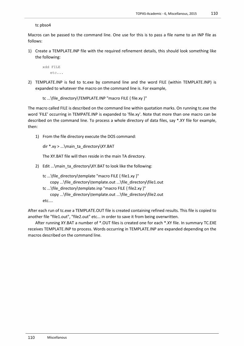
TOPAS-Academic - 6, Miscellanous, 2015 110
110 Miscellanous
tc pbso4
Macros can be passed to the command line. One use for this is to pass a file name to an INP file as
follows:
1) Create a TEMPLATE.INP file with the required refinement details, this should look something like
the following:
xdd FILE
etc...
2) TEMPLATE.INP is fed to tc.exe by command line and the word FILE (within TEMPLATE.INP) is
expanded to whatever the macro on the command line is. For example,
tc ...\file_directory\TEMPLATE.INP "macro FILE { file.xy }"
The macro called FILE is described on the command line within quotation marks. On running tc.exe the
word 'FILE' occurring in TEMPATE.INP is expanded to 'file.xy'. Note that more than one macro can be
described on the command line. To process a whole directory of data files, say *.XY file for example,
then:
1) From the file directory execute the DOS command:
dir *.xy > ...\main_ta_directory\XY.BAT
The XY.BAT file will then reside in the main TA directory.
2) Edit ...\main_ta_directory\XY.BAT to look like the following:
tc ...\file_directory\template "macro FILE { file1.xy }"
copy ...\file_directory\template.out ...\file_directory\file1.out
tc ...\file_directory\template.inp "macro FILE { file2.xy }"
copy ...\file_directory\template.out ...\file_directory\file2.out
etc....
After each run of tc.exe a TEMPLATE.OUT file is created containing refined results. This file is copied to
another file "file1.out", "file2.out" etc... in order to save it from being overwritten.
After running XY.BAT a number of *.OUT files is created one for each *.XY file. In summary TC.EXE
receives TEMPLATE.INP to process. Words occurring in TEMPLATE.INP are expanded depending on the
macros described on the command line.

TOPAS-Academic - 6, Keywords, 2015 111
111 Keywords
11 KEYWORDS
11.1 . Data structures
The following describes keyword dependencies. Trailing ‘…’ implies that more than one node of that
type can be inserted under its parent. Items enclosed in square brackets are optional. Items beginning
with a capital T corresponds to keyword groups analogous to complex types in XML.
Ttop Tcomm_1 Tcomm_2 Ttop_xdd Tglobal Txdd Txdd_scr Tindexing Tcharge_flipping
Ttop_xdd
[convolution_step #] [r_p #] [r_wp #] [r_exp #] [gof #] [r_p_dash #] [r_wp_dash #] [r_exp_dash #] [Rp !E] [Rs !E] [weighted_Durbin_Watson #] [x_calculation_step !E]
Tglobal
[A_matrix][C_matrix][A_matrix_normalized][C_matrix_normalized] [approximate_A]
[A_matrix_memory_allowed_in_Mbytes #] [A_matrix_elements_tollerance #] [A_matrix_report_on]
[bootstrap_errors !E] [fraction_of_yobs_to_resample !E] [determine_values_from_samples] [resample_from_current_ycalc]
[chi2 !E] [chi2_convergence_criteria !E] [conserve_memory] [continue_after_convergence] [do_errors] [do_errors_include_restraints] [do_errors_include_penalties] [file_name_for_best_solutions $file] [force_positive_fwhm] [iters #] [line_min] [use_extrapolation] [no_normal_equations] [use_LU] [marquardt_constant !E]… [no_LIMIT_warnings] [only_penalties] [out_A_matrix $file]
[A_matrix_prm_filter $filter] [out_refinement_stats] [out_rwp $file] [out_prm_vals_per_iteration $file]... | [out_prm_vals_on_convergence $file]...

TOPAS-Academic - 6, Keywords, 2015 112
112 Keywords
[out_prm_vals_filter $filter] [out_prm_vals_dependents_filter $filter_dependents]
[pen_weight !E] [penalties_weighting_K1 !E] [percent_zeros_before_sparse_A #] [process_times] [quick_refine !E [quick_refine_remove !E]] [randomise_file_out_normal $file] [randomize_on_errors] [restraint !E] [save_best_chi2] [seed] [temperature !E]...
[move_to_the_next_temperature_regardless_of_the_change_in_rwp] [save_values_as_best_after_randomization] [use_best_values]
[use_tube_dispersion_coefficients] [verbose #]
Txdd
[xdd $file [{$data}] [range #] [xye_format] [gsas_format] [fullprof_format] ]... Ttop_xdd Txdd_comm_1 Tcomm_1 Tcomm_2 Tmin_max_rc [elemental_composition] [element_weight_percent $atom . $Name #]… [element_weight_percent_known $atom #]… [gui_add_bkg !E] [mixture_MAC !E] [mixture_density_g_on_cm3 !E] [scale_phase_X E] [weight_percent_amorphous !E] [xdd_sum !E] [xo_Is]...
[xo E I E]... Tcomm_1_2_phase_1_2
[d_Is]... [d E I E]... Tcomm_1_2_phase_1_2 Tlebail
[hkl_Is]... [lp_search !E] [I_parameter_names_have_hkl $start_of_parameter_name] [hkl_m_d_th2 # # # # # # E I E]... [scale_phase_X E] Tspace_group Tcomm_1_2_phase_1_2 Thkl_lat Tlebail
[str | dummy_str]... Tstr_details Thkl_lat Tcomm_1_2_phase_1_2

TOPAS-Academic - 6, Keywords, 2015 113
113 Keywords
Tmin_max_rs Trigid [scale_phase_X E] Tspace_group
[user_y $Name { #include $Some_file }]… [user_y $Name $ Some_file]…
Tcomm_1_2_phase_1_2
Tcomm_1 Tcomm_2 Tphase_1 Tphase_2
Txdd_scr
[xdd_scr $file] … Txdd_comm_1 Tcomm_2 Ttop_xdd Tmin_max_r [dont_merge_equivalent_reflections] [dont_merge_Friedel_pairs] [ignore_differences_in_Friedel_pairs] [str]...
Tstr_details Tphase_1 Tcomm_2 Thkl_lat Tmin_max_r Trigid Tspace_group Tscr_1
Tscr_1
[Flack E] [i_on_error_ratio_tolerance #] [num_highest_I_values_to_keep #]
Txdd_comm_1
[bkg [@] # # #...] [d_spacing_to_energy_in_eV_for_f1_f11 !E] [exclude #ex1 #ex2]... [extra_X_left !E] [extra_X_right !E] [fit_obj E [min_X !E] [max_X !E] ]...
[fit_obj_phase !E] [fo_transform_X !E]
[neutron_data] [rebin_with_dx_of !E] [smooth #] [start_X !E] [finish_X !E] [weighting !E [recal_weighting_on_iter]] [xdd_out $file [append] ]...
Tout_record [yobs_eqn !N E] [yobs_to_xo_posn_yobs !E]

TOPAS-Academic - 6, Keywords, 2015 114
114 Keywords
Tcomm_1 [axial_conv]...
filament_length E sample_length E receiving_slit_length E [primary_soller_angle E] [secondary_soller_angle E] [axial_n_beta !E]
[capillary_diameter_mm E]... capillary_u_cm_inv E capillary_parallel_beam | capillary_divergent_beam
[lpsd_th2_angular_range_degrees E]... lpsd_equitorial_divergence_degrees E lpsd_equitorial_sample_length_mm E
[lpsd_beam_spill_correct_intensity !E] [circles_conv E]... [exp_conv_const E [exp_limit E] ]... [ft_conv !E]...
[ft_min !E] [ft_x_axis_range !E] ‘ Get(ft_0) ‘ FT_Break
[gauss_fwhm E]... [h1 E h2 E m1 E m2 E] [hat E [num_hats #] ]... [modify_peak]
[modify_peak_apply_before_convolutions] [modify_peak_eqn !E] [current_peak_min_x !E] [current_peak_max_x !E]
[more_accurate_Voigt] [lor_fwhm E]... [numerical_lor_gauss_conv] [numerical_lor_ymin_on_ymax #] [one_on_x_conv E]... [pk_xo E] [push_peak]…[bring_2nd_peak_to_top]…[add_pop_1st_2nd_peak]…[scale_top_peak E]… [pv_lor E pv_fwhm E] [spv_h1 E spv_h2 E spv_l1 E spv_l2 E] [stacked_hats_conv [whole_hat E [hat_height E]]...[half_hat E [hat_height E]]...]... [th2_offset E]... [user_defined_convolution E min E max E]... [WPPM_ft_conv E]…
WPPM_L_max E WPPM_th2_range E [WPPM_correct_Is]
Tcomm_2
[f0_f1_f11_atom]… [f0 E] [f1 E] [f11 E]
[lam [ymin_on_ymax #] [no_th_dependence] [Lam !E] [calculate_Lam]] [la E lo E [lh E] | [lg E] [lo_ref] ]...
[scale_pks E]... [prm|local E [min !E] [max !E] [del !E] [update !E] [stop_when !E] [val_on_continue !E]]... [existing_prm E] [penalty !E]...

TOPAS-Academic - 6, Keywords, 2015 115
115 Keywords
[out $file [append] ]... Tout_record
Tphase_1
[atom_out $file [append]]… Tout_record
[auto_scale !E] [cell_mass !E] [cell_volume !E] [weight_percent !E]
[spiked_phase_measured_weight_percent !E] [corrected_weight_percent !E] [del_approx !E] [phase_MAC !E] [phase_name $phase_name] [phase_out $file [append] ]... [brindley_spherical_r_cm !E] [r_bragg #] [remove_phase !E] [scale E]
Tphase_2
[peak_buffer_step E [report_on] ] [peak_type $type] [numerical_area E]
Tlebail
[lebail #] Tstr_details
[append_cartesian] [append_fractional [in_str_format] ] [append_bond_lengths [consider_lattice_parameters] ] [atomic_interaction N E] | [ai_anti_bump N]...
ai_sites_1 $sites_1 ai_sites_2 $sites_2 [ai_no_self_interation] [ai_closest_N !E] [ai_radius !E] [ai_exclude_eq_0] [ai_only_eq_0]
[box_interaction [from_N #] [to_N #] [no_self_interaction] $site_1 $site_2 N E]... [fourier_map !E]
[fourier_map_formula !E] [extend_calculated_sphere_to !E] [min_grid_spacing !E] [correct_for_atomic_scattering_factors !E] [f_atom_type $type [f_atom_quantity !E]]…
[grs_interaction [from_N #] [to_N #] [no_self_interaction] $site_1 $site_2 qi # qj # N E]... [hkl_plane $hkl]… [mag_only_for_mag_sites] [mag_space_group $symbol] [no_f11] [normalize_FCs] [occ_merge $sites [occ_merge_radius !E]]… [site $site]...
[x E] [y E] [z E] [num_posns #] [rand_xyz !E] [inter !E] [occ $atom E beq E]... [adps] [u11 E] [u22 E] [u33 E] [u12 E] [u13 E] [u23 E]

TOPAS-Academic - 6, Keywords, 2015 116
116 Keywords
Tmin_r_max_r [layer $layer_name] [mlx E] [mly E] [mlz E] [mg E] [mag_only]
[sites_distance N] | [sites_angle N] | [sites_flatten N [sites_flatten_tol !E]]... [site_to_restrain $site [ #ep [ #n1 #n2 #n3 ] ] ]...
[sites_geometry N]... [site_to_restrain $site [ #ep [ #n1 #n2 #n3 ] ] ]...
[siv_s1_s2 # #] [report_on_str] [stack $layer_name]...
[sx E] [sy E] [sz E] [generate_these $sites]
[generate_name_append $append_to_site_name] [view_structure]
Thkl_lat [a E] [b E] [c E] [al E] [be E] [ga E] [normals_plot !E]…
[normals_plot_min_d !E] [phase_penalties $sites N [hkl_Re_Im #h #k #l #Re #Im]...]…
[accumulate_phases_and_save_to_file $file] [accumulate_phases_when !E]
[spherical_harmonics_hkl $name]... [sh_Cij_prm $Yij E]... [sh_order #] [sh_alpha !E]
[str_hkl_angle N h k l]... [omit_hkls !E]
Trigid
[rigid]... [point_for_site $site [ux|ua E] [uy|ub E] [uz|uc E] ]...
[in_cartesian] [in_FC] [z_matrix $atom_1 [$atom_2 E] [$atom_3 E] [$atom_4 E] ] … [rotate E [qx|qa E] [qy|qb E] [qz|qc E] ]...
[operate_on_points $sites] [in_cartesian] [in_FC]
[translate [tx|ta E] [ty|tb E] [tz|tc E] ]... [operate_on_points $sites] [rand_xyz !E] [in_cartesian] [in_FC] [start_values_from_site $unique_site_name]
Tout_record
[out_record]… [out_eqn !E] [out_fmt $c_fmt_string] [out_fmt_err $c_fmt_string]...
Tmin_r_max_r
[min_r #] [max_r #] Tspace_group
[space_group $symbol]

TOPAS-Academic - 6, Keywords, 2015 117
117 Keywords
Miscellanous
[aberration_range_change_allowed !E] [default_I_attributes !E] load move_to for
11.2 . Alphabetical listing of keywords
[a E] [b E] [c E] [al E] [be E] [ga E]
Lattice parameters in Angstroms and lattice angles in degrees.
[adps] [u11 E] [u22 E] [u33 E] [u12 E] [u13 E] [u23 E]
adps when used generates the unn atomic displacement parameters with considerations made for
special positions. On termination of refinement the adps keyword is replaced with the unn
parameters; see example AE1-ADPS.INP. Instead of using the adps keyword the unn parameters
can be manually entered.
The unn matrix can be kept positive definite with the site dependent macro ADPs_Keep_PD;
this can stabilize refinement. The ADPs_Keep_PD macro can be used after the unn parameters are
created. For determining adp constraints the 3x3 eigen value determination routine of Kopp (2006)
has been used.
[A_matrix][C_matrix][A_matrix_normalized][C_matrix_normalized]
Generates the un-normalized and normalized A and correlation matrices. If do_errors is defined
then C_matrix_normalized is automatically generated and appeneded to the OUT file.
[append_cartesian] [append_fractional [in_str_format] ]
Appends site fractional coordinates in Cartesian or fractional coordinates respectively to the *.OUT
file at the end of a refinement. For the case of append_fractional, the in_str_format keyword
formats the output in INP format.
[append_bond_lengths [consider_lattice_parameters] ]
Appends bond lengths to the end of the *.OUT file at the end of refinement. A number
corresponding to equivalent positions is appended to site names.
consider_lattice_parameters includes the effects of lattice parameter errors in the calculation
of bond length and bond angle errors.
An example of bond lengths output is as follows:
Y1:0 O1:0 2.23143
O2:0 2.23143 88.083
O3:0 2.28045 109.799 99.928
The first line gives the distance between the sites Y1 and O2. The first number in the second line
gives the distance between sites Y1 and O2. The third number of 88.083 gives the angle between
the vectors Y1 to O1 and Y1 to O2. The first number on the third line contains the distance
between sites Y1 and O3. The second number in the third line contains the angle between the
vectors Y1 to O3 and Y1 to O2. The third number in line three contains the angle between the
vectors Y1 to O3 and Y1 to O1. Thus bond lengths correspond to the first number in each line and

TOPAS-Academic - 6, Keywords, 2015 118
118 Keywords
bond angles start from the second number. The numbers after the site name and after the ‘:’
character corresponds to the site equivalent position as found in the *.SG space group files found
in the SG directory
[approximate_A]
[A_matrix_memory_allowed_in_Mbytes !E]
[A_matrix_elements_tollerance !E]
[A_matrix_report_on]
See section 4.2 for a description of approximate_A.
A_matrix_memory_allowed_in_Mbytes limits the memory used by the A matrix to a maximum
of A_matrix_memory_allowed_in_Mbytes. If the matrix requires less than
A_matrix_memory_allowed_in_Mbytes then the full matrix is used otherwise the matrix is treated
as a sparse matrix.
A_matrix_elements_tollerance removes elements in the A matrix with values less than
A_matrix_elements_tollerance. The comparison is made againts normalized elements of A such
that the diagonals have a values of 1. The A matrix is made sparse when
A_matrix_elements_tollerance is defined. Typical values of A_matrix_memory_allowed_in_Mbytes
range from 0.0001 to 0.01.
A_matrix_memory_allowed_in_Mbytes and A_matrix_elements_tollerance can be used
simultanuously.
A_matrix_report_on displays the percentage of non-zero elements in the A matrix.
[atomic_interaction N E] | [ai_anti_bump N]...
ai_sites_1 $sites_1 ai_sites_2 $sites_2
[ai_no_self_interation]
[ai_closest_N !E]
[ai_radius !E]
[ai_exclude_eq_0]
[ai_only_eq_0]
Defines an atomic interaction with the name N between sites identified by $site_1 and $site_2. For
atomic_interaction E is the site interaction equation that can be a function of R and Ri. R returns
the distance in Å between two atoms; these distances are updated when dependent fractional
atomic coordinates are modified. The name of the atomic_interaction N can be used in equations
and in particular penalty equations.
For ai_anti_bump an anti-bump interaction equations is internally generated. For anti-
bumping only the ai_anti_bump is faster than using atomic_interaction. The macro AI_Anti_Bump
uses ai_anti_bump.
no_self_interaction prevents any interactions between equivalent positions of a site. This is
useful when a general position is used to describe a special position.
ai_closest_N: interactions between $sites_1 and $sites_2 are sorted by distance and only the
first ai_closest_N number of interactions are considered.
ai_radius: only the interactions between $sites_1 and $sites_2 that are within the distance
ai_radius are considered.
When ai_radius and ai_closest_N are both defined then interactions from both sets of
corresponding interaction are considered.
ai_exclude_eq_0: only interactions that is not the first equivalent positions in $sites_2 are
considered. For example, in the following:

TOPAS-Academic - 6, Keywords, 2015 119
119 Keywords
atomic_interaction...
ai_exclude_eq_0
ai_sites_1 Pb
ai_sites_1 “O1 O2”
the following interactions are considered:
Pb:0 and O1:n (n 0)
Pb:0 and O2:n (n 0)
where the number after the ‘:’ character corresponds to the equivalent positions of the sites.
ai_only_eq_0: only interactions between equivalent positions 0 are considered.
Functions
The atomic_interaction’ equation can be a function of the following functions:
AI_R(#ri): Returns the distance between the current site and the atom defined with Ri = #ri.
AI_R_CM: A function of no arguments that returns the geometric center of the current atom
and the atoms defined in $sites_2.
AI_Flatten(#toll): A function that returns the sum of distances of the current atom and those
defined in $sites_2 to an approximate plane of best fit. The plane of best fit is constructed such
that the sum of the perpendicular distances to the current atom plus those defined in $sites_2 are
a minimum
AI_Cos_Angle(#ri1, #ri2): Returns the Cos of the angle between the atom define as Ri=#ri1, the
current atom and the atom defined as Ri=#ri2.
AI_Angle(#ri1, #ri2) : Similar to AI_Cos_Angle except that the value returned is the angle in
degrees.
Examples BENZENE_AI1.INP, BENZENE_AI2.INP and BENZENE_AI3.INP demonstrates the use of
the atomic_interation functions.
atomic_interaction’s can be used to apply geometric restraints. For example, an anti-bump
interaction between symmetry related molecules can be formulated as follows:
atomic_interaction ai1 =
IF R < 3 THEN
(R-3)^2
ELSE
0
ENDIF
;
ai_exclude_eq_0
ai_sites_1 C*
ai_sites_1 C*
ai_radius 3
penalty = If(Cycle_Iter < 10, ai1, 0);
This example demonstrates anti-bumping between molecules for the first ten iterations of a
refinement cycle.
[atom_out $file [append] ]...
Used for writing site dependent details to file. See the keyword out for a description of out_record.
The Out_CIF_STR uses atom_out
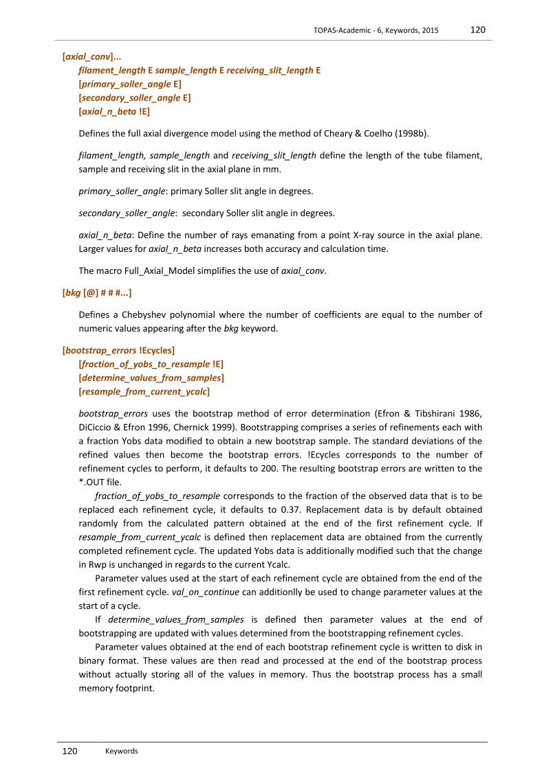
TOPAS-Academic - 6, Keywords, 2015 120
120 Keywords
[axial_conv]...
filament_length E sample_length E receiving_slit_length E
[primary_soller_angle E]
[secondary_soller_angle E]
[axial_n_beta !E]
Defines the full axial divergence model using the method of Cheary & Coelho (1998b).
filament_length, sample_length and receiving_slit_length define the length of the tube filament,
sample and receiving slit in the axial plane in mm.
primary_soller_angle: primary Soller slit angle in degrees.
secondary_soller_angle: secondary Soller slit angle in degrees.
axial_n_beta: Define the number of rays emanating from a point X-ray source in the axial plane.
Larger values for axial_n_beta increases both accuracy and calculation time.
The macro Full_Axial_Model simplifies the use of axial_conv.
[bkg [@] # # #...]
Defines a Chebyshev polynomial where the number of coefficients are equal to the number of
numeric values appearing after the bkg keyword.
[bootstrap_errors !Ecycles]
[fraction_of_yobs_to_resample !E]
[determine_values_from_samples]
[resample_from_current_ycalc]
bootstrap_errors uses the bootstrap method of error determination (Efron & Tibshirani 1986,
DiCiccio & Efron 1996, Chernick 1999). Bootstrapping comprises a series of refinements each with
a fraction Yobs data modified to obtain a new bootstrap sample. The standard deviations of the
refined values then become the bootstrap errors. !Ecycles corresponds to the number of
refinement cycles to perform, it defaults to 200. The resulting bootstrap errors are written to the
*.OUT file.
fraction_of_yobs_to_resample corresponds to the fraction of the observed data that is to be
replaced each refinement cycle, it defaults to 0.37. Replacement data is by default obtained
randomly from the calculated pattern obtained at the end of the first refinement cycle. If
resample_from_current_ycalc is defined then replacement data are obtained from the currently
completed refinement cycle. The updated Yobs data is additionally modified such that the change
in Rwp is unchanged in regards to the current Ycalc.
Parameter values used at the start of each refinement cycle are obtained from the end of the
first refinement cycle. val_on_continue can additionlly be used to change parameter values at the
start of a cycle.
If determine_values_from_samples is defined then parameter values at the end of
bootstrapping are updated with values determined from the bootstrapping refinement cycles.
Parameter values obtained at the end of each bootstrap refinement cycle is written to disk in
binary format. These values are then read and processed at the end of the bootstrap process
without actually storing all of the values in memory. Thus the bootstrap process has a small
memory footprint.

TOPAS-Academic - 6, Keywords, 2015 121
121 Keywords
[box_interaction [from_N #] [to_N #] [no_self_interaction] $site_1 $site_2 N E]...
Defines a site interaction with the name N between sites identified by $site_1 and $site_2. E
represents the site interaction equation which can be a function of R and Ri. R returns the distance
in Å between two atoms; these distances are updated when dependent fractional atomic
coordinates are modified. The name of the box_interaction N can be used in equations and in
particular penalty equations.
When either from_N or to_N are defined, the interactions between $site_1 and $site_2 are
sorted by distance and only the interactions between the from_N and to_N are considered.
no_self_interaction prevents any interactions between equivalent positions of the same site.
This is useful when a general position is used to describe a special position.
For example, the following could be used to iterate from the nearest atom to the third atom
from a site called Si1:
str
site Si1...
site O1...
site O2...
site O3...
box_interaction Si1 O* to_N 2 !si1o = (R-2)^2;
penalty = !si1o;
In this example the nearest three oxygen atoms are soft constrained to a distance of 2 Angstroms
by the use of the penalty function. Counting starts at zero and thus to_N is set to 2 to iterate up to
the third nearest atom.
The wild card character ‘*’ used in “O*” means that sites with names starting with ‘O’ are
considered. In addition to using the wild card character, the site names can be explicitly written
within double quotation marks, for example:
box_interaction Si1 “O1 O2 O3” to_N 3 etc...
Interactions between Si1 and the three oxygen atoms O1, O2, O3 may not all be included, for
example, if Si1 had as its nearest neighbours the following:
Si1 ↔ O1,1 at a distance of 1.0 Angstroms
Si1 ↔ O2,3 at a distance of 1.1 Angstroms
Si1 ↔ O2,1 at a distance of 1.2 Angstroms
Si1 ↔ O1,2 at a distance of 1.3 Angstroms
then two equivalent positions of site O1 and two equivalent positions of O2 are included in the
interaction equation; thus no interaction between Si1-O3 is considered. To ensure that each of the
three oxygens had Si1 included in an interaction equation then the following could be used:
box_interaction “O1 O2 O3” Si1 to_N 0 etc…
Thus the order of $site_1 and $site_2 is important when either from_N or to_N is defined.
The reserved parameters Ri and Break can also be used in interaction equations when either
from_N or to_N is defined. Ri returns the index of the current interaction being operated on with
the first interaction starting at Ri=0.
box_interaction is used for example in the Anti_Bump macro.

TOPAS-Academic - 6, Keywords, 2015 122
122 Keywords
[brindley_spherical_r_cm !E]
Used for applying the Brindley correction for spherical particles. The macro
Apply_Brindley_Spherical_R_PD(R, PD) is defined as:
macro Apply_Brindley_Spherical_R_PD(R, PD) {
brindley_spherical_r_cm = (R) (PD);
}
R is the radius of the particle in cm and PD is the packing density, a number that is not updated
and not refined. Here’s an example:
xdd...
str
Apply_Brindley_Spherical_R_PD(R, PD)
MVW(0,0,0)
str
Apply_Brindley_Spherical_R_PD(R, PD)
MVW(0,0,0)
Note, that PD is incorporated by way of an equation definition for brindley_spherical_r_cm. Also,
phase_MAC or MVW need not be defined as they are created as needed; their definition however
is necessary in order to obtain their respective values. The Brindley correction is not applied to
phases without the brindley_spherical_r_cm defined.
The Brindley correction can be applied to all phases including xo_Is. In the case of phases that
do not have lattice parameters or sites then the User would need to enter values for cell_volume,
cell_mass and phase_MAC in order for the Brindley correction to work and for the weight percents
to be obtained. This allows for the incorporation of non-structural phases in quantitative analysis.
For example, the following works as the necessary information have been included.
xo_Is
Apply_Brindley_Spherical_R_PD(.002, .6)
MVW(654, 230, 0)
phase_MAC 200
[capillary_diameter_mm E]...
capillary_u_cm_inv E
capillary_parallel_beam | capillary_divergent_beam
Calculates an aberration for capillary samples. and convolutes it into phase peaks.
capillary_diameter_mm corresponds to the capillary diameter in mm and capillary_u_cm_inv the
linear absorption coefficient of the sample in units of cm-1. The capillary_diameter_mm
convolution corrects for peak shapes, intensities and 2Th shifts, see example CAPILLARY-
SIMULATED.INP.
Use of capillary_parallel_beam results in a correction for a parallel primary beam.
Use of capillary_divergent_beam results in a correction for a divergent primary beam.
Both capillary_parallel_beam and capillary_divergent_beam assume that the capillary is fully
illuminated by the beam in the equitorial plane.
TOPAS-Academic - 6, Keywords, 2015 123
123 Keywords
[cell_mass !E] [cell_volume !E] [weight_percent !E]
[spiked_phase_measured_weight_percent !E] [corrected_weight_percent !E]
cell_mass, cell_volume and weight_percent correspond to unit cell mass, volume and weight
percent of the phase within the mixture.
spiked_phase_measured_weight_percent defines the weight percent of a spiked phase. Used
by the xdd dependent keyword weight_percent_amorphous to determine amorphous weight
percent. Only one phase per xdd is allowed to contain the keyword
spiked_phase_measured_weight_percent.
corrected_weight_percent is the weight percent after considering amorphous content as
determined by weight_percent_amorphous.
The weight fraction wp for phase "p" is calculated as follows:
pN
1p
p
p
p
Q
Q w
where Np = Number of phases
Qp = SpMpVp/Bp
Sp = Rietveld scale factor for phase p.
Mp = Unit cell mass for phase p.
Vp = Unit cell volume for phase p.
Bp = Brindley correction for phase p
The Brindley correction is a function of brindley_spherical_r_cm and the phase and mixture linear
absorption coefficients; the latter two are in turn functions of phase_MAC and mixture_MAC
respectively, or,
Bp is function of : (LACphaseMACmixture) brindley_spherical_r_cm
where
LACphase = linear absorption coefficient of phase p, packing density of 1.
MACmixture = linear absorption coefficient of the mixture, packing density of 1.
This makes Bp a function of the weight fractions wp of all phases and thus wp as written above
cannot be solved analytically. Subsequently wp is solved numerically through the use of iteration.
[chi2_convergence_criteria !E]
Convergence is determined when the change in 2 is less than chi2_convergence_criteria for
three consecutive cycles and when all defined stop_when parameter attributes evaluate to true.
Example:
chi2_convergence_criteria = If(Cycle_Iter < 10, .001, .01);
[circles_conv E]...
Defines m in the convolution function:
(1 m / ½) for = 0 to m
that is convoluted into phase peaks. m can be greater than or less than zero. circles_conv is used
for example by the Simple_Axial_Model macro.

TOPAS-Academic - 6, Keywords, 2015 124
124 Keywords
[cloud $sites]...
[cloud_population !E]
[cloud_save $file]
[cloud_save_xyzs $file]
[cloud_load_xyzs $file]
[cloud_load_xyzs_omit_rwps !E]
[cloud_formation_omit_rwps !E]
[cloud_try_accept !E]
[cloud_gauss_fwhm !E]
[cloud_extract_and_save_xyzs $file]
[cloud_number_to_extract !E]
[cloud_atomic_separation !E]
cloud allows for the tracking of atoms defined in $sites in three dimensions. It can be useful for
determining the average positions of heavy atoms or rigid bodies during refinement cycles. For
example, a dummy atom, “site X1” say, can be placed at the center of a benzene ring and then
tracked as follows:
continue_after_convergence
…
cloud “X1”
cloud_population 100
cloud_save SOME_FILE.CLD
On termination of refinement the CLD file is saved; it can be viewed using the rigid body editor of
the GUI; see examples AE14-12.INP for a cloud example. cloud_population is the maximum
number of population members. Each population member comprises the fractional coordinates of
$sites and an associated Rwp value.
cloud_save_xyzs saves a cloud populations to file.
cloud_load_xyzs loads and reuses previously saved populations. cloud_load_xyzs_omit_rwps can
be used to exclude population membes whilst loading; it can be a function of Get(Cloud_Rwp)
where Cloud_Rwp is the associated Rwp of a population member.
cloud_formation_omit_rwps can be used to limit population membes in the formation of CLD
files; it can be a function of Get(Cloud_Rwp).
cloud_try_accept accepts population members if it evaluates to non-zero and if the best Rwp
since the last acceptance is less than a present population member or if the number of members is
less than cloud_population. If the number of population members equals cloud_population then
the population member with the lowest Rwp is discarded. cloud_try_accept is evaluated at the
end of each refinement cycle; it default value is true. Here’s are some examples:
cloud_try_accept = And(Cycle, Mod(Cycle, 50);
cloud_try_accept = T == 10;
cloud_gauss_fwhm is the full width at half maximum of a three dimensional Gaussian that is used
to fill the cloud.
cloud_extract_and_save_xyzs searches the three dimensional cloud for high densities and
extracts xyz positions; these are then saved to $file. cloud_number_to_extract defines the number
of positions to extract and cloud_atomic_separation limits the atomic separation during the
extraction. The actual number of positions extracted may be less than cloud_number_to_extract
depending on the cloud.
TOPAS-Academic - 6, Keywords, 2015 125
125 Keywords
[conserve_memory]
Deletes temporary arrays used in intermediate calculations; memory savings of up to 70% can be
expected on some problems with subsequent lengthening of execution times by up to 40%. When
approximate_A is used on dense matrices then conserve_memory can reduce memory usage by
up to 90%.
[continue_after_convergence]
Refinement is continued after convergence. Before continuing the following actions are
performed:
val_on_continue equations for independent parameters are evaluated
randomize_on_errors process is performed
rand_xyz processes are performed
Also, when val_on_continue is defined then the corresponding parameter is not randomized
according to randomize_on_errors.
[convolution_step #]
An integer defining the number of calculated data points per measured data point. It may be
useful to increase this number when the measurement step is large. convolution_step is set to 1 by
default. Only when the measurement step is greater than about 0.03 degrees 2Th or when high
precision is required is it necessary to increase convolution_step.
[default_I_attributes E]
Changes the attributes of the I parameter, for example,
xo_Is
default_I_attributes 0 min 0.001 val_on_continue 1
Useful when randomising lattice parameters during Le Bail refinements with
continue_after_convergence.
[d_Is]...
[d E I E]...
Defines a phase type that uses d-spacing values for generating peak positions. d corresponds to
the peak position in d-space in Å and I is the intensity parameter before applying any scale_pks
equations.
[do_errors]
Errors for refined parameters (ESD's) and a correlation matrix are calculated at the end of
refinement. The correlation matrix if defined using C_matrix_normalized is updated, if not defined
then C_matrix_normalized is automatically defined and appeneded to the OUT file.
[d_spacing_to_energy_in_eV_for_f1_f11 !E]
Can be a function of the reserved parameter D_spacing. Changes f' and f" (see section 10.5) to
correspond to energies as given by d_spacing_to_energy_in_eV_for_f1_f11. Used for refining on
energy dispersive data, for example,

TOPAS-Academic - 6, Keywords, 2015 126
126 Keywords
' E(eV) = 10^5 / (8.065541 Lambda(A))
prm !detector_angle_in_radians = 7.77 Deg_on_2;
prm wavelength = 2 D_spacing Sin(detector_angle_in_radians);
prm energy_in_eV = 10^5 / (8.065541 wavelength);
pk_xo = 10^-3 energy_in_eV + zero;
d_spacing_to_energy_in_eV_for_f1_f11 = energy_in_eV;
See example ED_SI_STR.INP.
[exclude #ex1 #ex2]...
Excludes an x-axis region between #ex1 and #ex2. The macro "Exclude" simplifies the use of
exclude. Example CEO2.INP demonstrates the use of excluded regions.
[exp_conv_const E [exp_limit E] ]...
Defines m in the convolution function:
Exp(Ln(0.001) m) for = 0 to exp_limit
that is convoluted into phase peaks. exp_conv_const is used by the Absorption and
Absorption_With_Sample_Thickness_mm macros (see example LI025.INP). If exp_limit is not
defined then it defaults to m. m can be greater than or less than zero.
[extra_X_left !E] [extra_X_right !E]
Determines the extra range to which hkls are generated. For TOF data extra_X_left is typically
used. For x-ray data then extra_X_right is typically used. Both default to 0.5.
[file_name_for_best_solutions $file]
Appends INP file details to $file during refinement with independent parameter values updated.
The operation is performed every time a particular convergence gives the best Rwp. For example,
suppose that at convergence the following was obtained:
Rwp:
30 All prms appended to file in INP format
20 All prms appended to file in INP format
35
40
15 All prms appended to file in INP format
18
10 All prms appended to file in INP format
15
[force_positive_fwhm]
Forces final Lorentzian and/or Gaussian FWHM values to be positive for a particular peak. The
following INP snippets are equivalent:
force_positive_fwhm
xdd
str
lor_fwhm = Rand(-1,1);
and:

TOPAS-Academic - 6, Keywords, 2015 127
127 Keywords
xdd
str
lor_fwhm = Abs(Rand(-1.1,));
[fit_obj E [min_X !E] [max_X !E] ]...
fit_obj's allows the insertion of User defined functions, see example PVS.INP. fit_obj’s can be a
function of X.
min_X and max_X define the x-axis range of the fit_obj; if min_X is omitted then the fit_obj is
calculated from the start of the x-axis; similarly if max_X is omitted then the fit_obj is calculated to
the end of the x-axis.
[fourier_map !E]
[fourier_map_formula !E]
[extend_calculated_sphere_to !E]
[min_grid_spacing !E]
[correct_for_atomic_scattering_factors !E]
[f_atom_type $type f_atom_quantity !E]…
If fourier_map is non-zero then a Fourier map is calculated on refinement termination and shown
in the OpenGL window; maps can be calculated for x-ray or neutron single crystal or powder data,
see test examples FOURIER-MAP-AE14.INP and FOURIER-MAP-CIME.INP. The type of map is
determined by fourier_map_formula which can be a function of the reserved parameter names
Fcalc, Fobs and D_spacing; here are some examples:
fourier_map_formula = Fobs; ‘ The default
fourier_map_formula = 2 Fobs - Fcalc;
Fobs corresponds to the obserbed structure moduli; in the powder data case Fobs is calculated
from the Rietveld decomposition formula. Phases are determined from Fcalc.
Reflections that are missing from within the Ewald sphere are included with Fobs set to Fcalc.
If extend_calculated_sphere_to is defined then the Ewald sphere is extended.
scale_pks definitions are removed from Fobs. In the event that scale_pks evaluates to zero for
a particular reflection then Fobs is set to Fcalc; the number of Fobs reflections set to Fcalc is
reported on.
[gauss_fwhm E]...
Defines the FWHM of a Gaussian function to be convoluted into phase peaks. gauss_fwhm is used
for example by the CS_G and Strain_G macros.
[hkl_plane $hkl] ...
Used by the OpenGL viewer to display hkl planes, see the CeO2.STR file in the “Rigid” directory.
Here are some examples:
str…
hkl_plane 1 1 1
hkl_plane “2 -2 0”
[grs_interaction [from_N #] [to_N #] [no_self_interaction] $site_1 $site_2 qi # qj # N E]...
Defines a GRS interaction with a name of N between sites identified by $site_1 and $site_2. E
represents the GRS interaction equation that can be a function of R, which returns the distance in
Angstroms between two atoms; these distances are updated when dependent fractional atomic

TOPAS-Academic - 6, Keywords, 2015 128
128 Keywords
coordinates are modified. The name of the grs_interaction N can be used in equations and in
particular penalty equations.
When either from_N or to_N are defined, the interactions between $site_1 and $site_2 are
sorted by distance and only the interactions between the from_N and to_N are considered.
no_self_interaction prevents any interactions between equivalent positions of the same site.
This is useful when a general position is used to describe a special position.
qi and qj corresponds to the valence charges used to calculate the Coulomb sum for the sites
$site_1 and $site_2 respectively.
grs_interaction is typically used for applying electrostatic restraints in inorganic materials. The
GRS_Interaction macro simplifies the use of grs_interaction.
[hat E [num_hats #] ]...
Defines the X-axis size of an impulse function that is convoluted into phase peaks. num_hats
corresponds to the number of hats to be convoluted. num_hats is set to 1 by default. hat is used
for example by the Slit_Width and Specimen_Tilt macros.
[hkl_Is]...
[lp_search !E]
[I_parameter_names_have_hkl $start_of_parameter_name]
[hkl_m_d_th2 # # # # # # I E]...
Defines a phase type that uses hkls for generating peak positions.
lp_search uses a new indexing algorithm that is independent of d-spacing extraction; LP-
SEARCH-PBSO4.INP demonstrates its use. lp_search minimizes on a new figure of merit function
that gives a measure of correctness for a particular set of lattice parameters. More specifically the
figure of merit function assigns parts of the diffraction pattern to peaks and then sums the
absolute values of the products of the diffraction intensities multiplied by the distance to the
peaks:
j i
j0,2 2 2I FOM ii
where the summation in ‘j’ is over the calculated Bragg positions 2 and the summation in ‘i’ is
over part of the diffraction pattern such that (2, j-1 + 2, j)/2 2i (2, j+1 + 2, j)/2. The
method avoids difficulties associated with extracting d-spacings from complex patterns comprising
heavily overlapped lines; the primary difficulty being that of ascertaining the number of lines
present.
I_parameter_names_have_hkl gives generated Intensity parameters a name starting with
$start_of_parameter_name and ending with the corresponding hkl.
hkl_m_d_th2: The numbers after the keyword hkl_m_d_th2 define h k l m d and 2 values, where
h, k, l : Miller indices
m : multiplicity.
d and th2 : d and 2 values (not used by).
I : Peak intensity parameter before applying any scale_pks.
If no hkl_m_d_th2 keywords are defined then the hkls are generated using the space group; the
generated hkl_m_d_th2 details are appended at the end of the space_group keyword on
refinement termination. Intensity parameters are given an initial starting value of 1. If the Le Bail
keyword is not defined then the intensity parameters are given the unique code of @ .

TOPAS-Academic - 6, Keywords, 2015 129
129 Keywords
For example, the following input segment:
xdd quartz.xdd
...
hkl_Is
Hexagonal(4.91459, 5.40603)
space_group P_31_2_1
will generate the following OUT file:
xdd quartz.xdd
...
hkl_Is
Hexagonal(4.91459, 5.40603)
space_group P_31_2_1
load hkl_m_d_th2 I
{
1 0 0 6 4.25635 20.85324 @ 3147.83321
1 0 1 6 3.34470 26.62997 @ 8559.23955
1 0 -1 6 3.34470 26.62997 @ 8559.23955
...
}
The Create_hklm_d_Th2_Ip_file macro creates an hkl file listing from structures in the same
format as the "load hkl_m_d_th2 I" as shown above. Even though the structure would have no
sites, the weight_percent keyword can still be used; it will use whatever value is defined by
cell_mass in order to calculate weight_percent.
[iters #]
The maximum number of refinement iterations, iters is set to 500000 by default
[lam [ymin_on_ymax #] [no_th_dependence] [Lam !E] [calculate_Lam]]
[la E lo E [lh E] | [lg E] [lo_ref] ]...
Defines an emission profile where each "[la E lo E [lh E] | [lg E] ]" determines an emission profile
line, where
la: Area under the emission profile line
lo: Wavelength in [Å] of the emission profile line
lh: HW in mÅ of a Lorentzian convoluted into the emission profile line.
lg: HW in mÅ of a Gaussian convoluted into the emission profile line.
ymin_on_ymax determines the x-axis extent to which an emission profile line is calculated. It is set
to 0.001 by default.
no_th_dependence defines an emission profile that is 2 independent. Allows the use of non-
X-ray data or fitting to negative 2 values.
Lam defines the value to be used for the reserved parameter Lam. When Lam is not defined
then the reserved parameter Lam is defined as the wavelength of the emission profile line with the
largest la values. Note that Lam is used to determine the Bragg angle.
calculate_Lam calculates Lam such that it corresponds to the wavelength at the peak of the
emission profile. Lam needs to be set to an approximate value corresponding to the peak of the
emission profile.

TOPAS-Academic - 6, Keywords, 2015 130
130 Keywords
By default the program calculates d-spacings using the wavelength of the emission profile line
with the highest la parameter. However, if la parameters are refined the reference wavelength
could change causing confusion. To avoid this lo_ref can be used to identify the reference
wavelength.
See section 5 for a description of emission profiles.
[lebail #]
A 1 for the lebail keyword flags the use of the Le Bail method for peak intensity extraction.
[line_min] [use_extrapolation] [no_normal_equations] [use_LU]
no_normal_equations prevents the use of normal equations in the minimization routine; it is
useful when the effects of line minimization only is sought or when there are a large number of
parameters being refined. Refer to section 4 for a description of the minimization routines .
[lor_fwhm E]...
Defines the FWHM of a Lorentzian function that is convoluted into phase peaks. lor_fwhm is used
for example by the CS_L and Strain_L macros.
[lpsd_th2_angular_range_degrees E]...
lpsd_equitorial_divergence_degrees E
lpsd_equitorial_sample_length_mm E
Calculates an aberration for a Linear Position Sensitive Detector (Cheary & Coelho, 1994) and
convolutes it into phase peaks. lpsd_th2_angular_range_degrees corresponds to the angular range
of the LPSD in 2Th degrees. lpsd_equitorial_divergence_degrees the equitorial divergence in
degrees of the primary beam and lpsd_equitorial_sample_length_mm is the lengths of the sample
in the equitorial plane.
The lpsd_th2_angular_range_degrees convolution corrests for peak shapes, intensities and
2Th shifts; see example LPSD-SIMULATED.INP.
[marquardt_constant !E]…
Allows for changing the Marquardt constants, the Simulated_Annealing_1 macro changes the
Marquardt constants as follows:
load marquardt_constant { 0 1 }
[min_r #] [max_r #]
Defines the minimum and maximum radii for calculating bond lengths. min_r and max_r are by
default set to 0 and 3.2 Å respectively.
[mixture_density_g_on_cm3 !E]
Calculates the density of the mixture assuming a packing density of 1, see also mixture_MAC.
[mixture_MAC !E]
Calculates the mass absorption coefficient in cm2/g for a mixture as follows:
iimixture w
N
1i
TOPAS-Academic - 6, Keywords, 2015 131
131 Keywords
where wi and (/)i is the weight percent and phase_MAC of phase i respectively. Errors are
reported for phase_MAC and mixture_MAC.
The following example provides phase and mixture mass absorption coefficients.
xdd...
mixture_MAC 0
str...
phase_MAC 0
The macros Mixture_LAC_1_on_cm, Phase_LAC_1_on_cm and Phase_Density_g_on_cm3
calculates the mixture and phase linear absorption coefficients (for a packing density of 1) and
phase density, for example:
xdd...
Mixture_LAC_1_on_cm(0)
str...
Phase_Density_g_on_cm3(0)
Phase_LAC_1_on_cm(0)
Errors for these quantities are also calculated. Mass absorption coefficients obtained from NIST at
http://physics.nist.gov/PhysRefData/XrayMassCoef are used to calculate mixture_MAC and
phase_MAC.
[neutron_data]
Signals the use of neutron atomic scattering lengths. Scattering lengths for isotopes can be used by
placing the isotope name after “occ” as in:
occ 6Li 1
occ 36Ar 1
The scattering lengths data, contained in the file NEUTSCAT.CPP, is from
www.ccp14.ac.uk/ccp/web-mirrors/neutrons/n-scatter/n-lengths/LIST~1.HTM
Constant wavelength neutron diffraction requires a Lorentz correction using the Lorentz_Factor
macro (defined in TOPAS.INC); it is defined as follows:
scale_pks = 1 / (Sin(Th)^2 Cos(Th));
[no_LIMIT_warnings]
Surpresses LIMIT_MIN and LIMIT_MAX warning messages.
[normalize_FCs]
If defined then site fractional coordinates are normalized. Normalization of a particular fractional
coordinate does not occur if it has min/max limits, is part of a rigid body or part of a site constraint
of any kind.
[numerical_area E]
Returns the numerically calculated area under the phase.

TOPAS-Academic - 6, Keywords, 2015 132
132 Keywords
[occ_merge $sites [occ_merge_radius !E]]...
occ_merge rewrites the site occupancy of the sites defined in $sites in terms of their fractional
atomic coordinates (Favre-Nicolin and R. Cerny 2002). This is useful during structure solution for
merging ocathedra or other types of defined rigid bodies. It is also useful for identifying special
positions as seen in the example PBSO4-DECOMPOSE.INP.
In the present implementation $sites are thought of as spheres with a radius
occ_merge_radius. When two atoms approach within a distance less than the sum of their
respective occ_merge_radius’s then the spheres intersect. The occupancies of the sites, occ_xyz,
thus become:
occ_xyz = 1 / (1 + Intersection fractional volumes)
In this way any number of sites can be merged.
Sites appearing in $sites cannot have their occupancies refined. On termination of refinement
the occ parameter values are updated with their corresponding occ_xyz.
[omit_hkls !E]
Allows for the filtering of hkls using the reserved parameter names of H, K, L and D_spacing. More
than one omit_hkls can be defined, for example:
omit_hkls = If(And(H==0, K==0), 1, 0);
omit_hkls = And(H==0, K==1);
omit_hkls = D_spacing < 1;
[one_on_x_conv E]...
Defines m in the convolution function:
(4 m ½ for = 0 to m
that is convoluted into phase peaks. m can be greater than or less than zero. one_on_x_conv is
used for example by the Divergence macro.
[only_penalties]
Instructs the minimization procedure to minimize on penalty functions only. The only_penalties
switch is assumed when there are only penalties to minimize, i.e. when there are no observed
data. Note, parameters that are not functions of penalties are not refined.
[out_A_matrix $file]
[A_matrix_prm_filter $filter]
out_A_matrix outputs the least squares A matrix to the file $file; used in the Out_for_cf macro.
Output can be limited by using A_matrix_prm_filter, here’s an example for outputting A matrix
elements corresponding to parameters with names starting with ‘q’:
out_A_matrix file.a
A_matrix_prm_filter q*
TOPAS-Academic - 6, Keywords, 2015 133
133 Keywords
[out $file [append] ]...
[out_record]
[out_eqn !E]
[out_fmt $c_fmt_string]
[out_fmt_err $c_fmt_string]...
Used for writing parameter details to a file. The details are appended to $file when append is
defined. out_eqn defines the equation or parameter to be written to $file using the out_fmt.
$c_fmt_string describes a format string in c syntax containing a single format specified for a double
precision number. out_fmt_err defines the $c_fmt_string used for formatting the error of eqn.
Both out_fmt and out_fmt_err requires an out_eqn definition. out_fmt can be used without
out_eqn for writing strings. The order of out_fmt and out_fmt_err determines which is written to
file first; thus if out_fmt_err is defined first then it will be operated on first.
The following example illustrates the use of out using the Out macros.
xdd...
out "sample output.txt" append
str...
CS_L(cs_l, 1000)
Out_String("\tCrystallite Size Results:\n")
Out_String("\t=========================\n")
Out(cs_l, "\tCrystallite Size (nm):\t%11.5f",
"\tError in Crystallite Size:\t%11.5f\n")
out provides a means of defining individual refinement result files, see example OUT-1.INP.
[out_rwp $file]
Outputs a list of Rwp values encountered during refinement to the file $file.
[out_prm_vals_per_iteration $file]... | [out_prm_vals_on_convergence $file]...
[out_prm_vals_filter $filter]
[out_prm_vals_dependents_filter $filter_dependents]
Outputs refined independent parameter values per iteration or on convergence into the file $file.
In the absence of out_prm_vals_filter then all parameters are outputted otherwise only
parameters with names defined in out_prm_vals_filter are considered where $fliter can contain
the wild card charatcter ’*’ and the negation character ’!’, for example:
out_prm_vals_per_iteration PRM_VALES.TXT
out_prm_vals_filter "* !u*"
More than one out_prm_vals_per_iteration/out_prm_vals_on_convergence can be defined
outputting different parameters into different files depending on the corresponding
out_prm_vals_filter.
out_prm_vals_dependents_filter allows dependent parameters to be outputted accoring to
$filter_dependents.
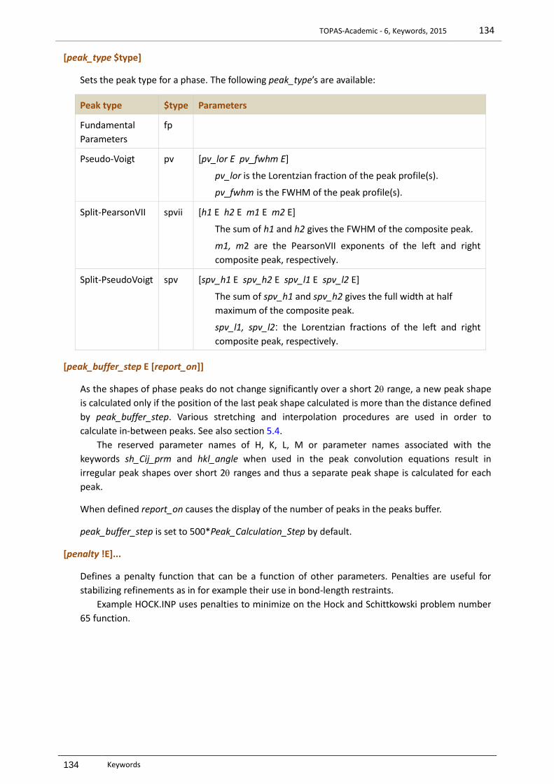
TOPAS-Academic - 6, Keywords, 2015 134
134 Keywords
[peak_type $type]
Sets the peak type for a phase. The following peak_type’s are available:
Peak type $type Parameters
Fundamental
Parameters
fp
Pseudo-Voigt
pv [pv_lor E pv_fwhm E]
pv_lor is the Lorentzian fraction of the peak profile(s).
pv_fwhm is the FWHM of the peak profile(s).
Split-PearsonVII
spvii [h1 E h2 E m1 E m2 E]
The sum of h1 and h2 gives the FWHM of the composite peak.
m1, m2 are the PearsonVII exponents of the left and right
composite peak, respectively.
Split-PseudoVoigt
spv [spv_h1 E spv_h2 E spv_l1 E spv_l2 E]
The sum of spv_h1 and spv_h2 gives the full width at half
maximum of the composite peak.
spv_l1, spv_l2: the Lorentzian fractions of the left and right
composite peak, respectively.
[peak_buffer_step E [report_on]]
As the shapes of phase peaks do not change significantly over a short 2 range, a new peak shape
is calculated only if the position of the last peak shape calculated is more than the distance defined
by peak_buffer_step. Various stretching and interpolation procedures are used in order to
calculate in-between peaks. See also section 5.4.
The reserved parameter names of H, K, L, M or parameter names associated with the
keywords sh_Cij_prm and hkl_angle when used in the peak convolution equations result in
irregular peak shapes over short 2 ranges and thus a separate peak shape is calculated for each
peak.
When defined report_on causes the display of the number of peaks in the peaks buffer.
peak_buffer_step is set to 500*Peak_Calculation_Step by default.
[penalty !E]...
Defines a penalty function that can be a function of other parameters. Penalties are useful for
stabilizing refinements as in for example their use in bond-length restraints.
Example HOCK.INP uses penalties to minimize on the Hock and Schittkowski problem number
65 function.
TOPAS-Academic - 6, Keywords, 2015 135
135 Keywords
prm x1 1 min -4.5 max 4.5 val_on_continue = Rand(-4.5, 4.5); del .01
prm x2 1 min -4.5 max 4.5 val_on_continue = Rand(-4.5, 4.5); del .01
prm x3 1 min -5.0 max 5.0 val_on_continue = Rand(-5.0, 5.0); del .01
' Hock and Schittkowski problem number 65 function
penalty = (x1-x2)^2 + (1/9) (x1 + x2 - 10)^2 + (x3 - 5)^2; : 0
prm contraint_1 = x1^2 + x2^2 + x3^2;
penalty = If(contraint_1 < 48, 0, (contraint_1-48)^2); : 0
The next example applies a User defined penalty function to lattice and crystallite size parameters,
which are expected to be 5.41011 Å and 200 nm respectively:
str...
Cubic(lp_ceo2 5.41011)
penalty = (lp_ceo2-5.41011)^2;
CS_L(cs_l, 200)
penalty =(cs_l-200)^2;
Minimizing on penalty functions in the presence of observed data is possible with the use of the
only_penalties keyword.
[penalties_weighting_K1 !E]
Defines the weighting K1 given to penalty functions as defined in Eq. (4-3). penalties_weighting_K1
is set to 1 by default.
[percent_zeros_before_sparse_A #]
Defines the percentage of the A matrix than can be zero before sparse matrix methods are
invoked. The default value is 60%.
[phase_MAC !E]
Calculates the mass absorption coefficient in cm2/g for the current phase. See description for
mixture_MAC.
[phase_out $file [append] ]...
Used for writing phase dependent details to file. See the keyword out for a description of
out_record. The Create_hklm_d_Th2_Ip_file uses phase_out.
[pk_xo E]
pk_xo is applied to all phase types except for xo_Is phases. It provides a mechanism for
transforming peak position to an x-axis position. For example, the peak position for neutron time-
of-flight data is typically calculated in time-of-flight space, tof, or:
tof = t0 + t1 dhkl + t2 dhkl2
where t0 and t1 and t2 are diffractometer constants. pk_xo can be used to refine TOF data as
shown in examples TOF_BALZAR_SH1.INP and TOF_BALZAR_BR1.INP.
[phase_name $phase_name]
The name given to a phase; used for reporting purposes.

TOPAS-Academic - 6, Keywords, 2015 136
136 Keywords
[phase_penalties $sites N]...[hkl_Re_Im #h #k #l #Re #Im]...
[accumulate_phases_and_save_to_file $file]
[accumulate_phases_when !E]
phase_penalties for a single hkl is defined as follows:
45 or,,45 phase theif ,)(I
45 45 phase theif ,0 Pp
,,
2
,,
2
hklc,
,,
hkl
hklschklschklchkls
hklschkls
d
where s = assigned phase, c = calculated phase, Ic = calculated intensity and d is the reflection
d-spacing. The name N returns the sum of the phase_penalties and it can be used in equations
and in particular penalty equations. c is calculated from sites identified in $sites.
#h, #k, #l are user defined hkls; they are used for formulating the phase penalties. #Re and #Im
are the real and imaginary parts of s . An example use of phase penalties (see examples AE14-
12.INP and AE5-AUTO.INP) is as follows:
penalty = pp1;
phase_penalties * pp1
load hkl_Re_Im
{
0 1 2 1 0
1 0 -2 1 0
1 -2 -1 1 0
}
hkls chosen for phase penalties should comprise those that are of high intensity, large d-spacing
and isolated from other peaks to avoid peak overlap. Origin defining hkls are typically chosen.
accumulate_phases_and_save_to_file saves the average phases collected to $file. Phases are
collected when accumulate_phases_when evaluates to true; accumulate_phases_when defaults to
true. Here’s an example use:
temperature 1
temperature 1
temperature 1
temperature 1
temperature 10
...move_to_the_next_temperature_regardless_of_the_change_in_rwp
accumulate_phases_and_save_to_file SOME_FILE.TXT
accumulate_phases_when = T == 10;
Here phases with the best Rwp since the last accumulation are accumulated when the current
temperature is 10.
[process_times]
Displays process times on termination of refinement.
[quick_refine !E [quick_refine_remove !E]]
quick_refine removes parameters that influence 2 in a small manner during a refinement cycle. Use
of quick_refine speeds up simulated annealing, see for example the macro Auto_T which is used in
example AE1-AUTO.INP. All refined parameters are reinstated for refinement at the start of subsequent
TOPAS-Academic - 6, Keywords, 2015 137
137 Keywords
cycles. Large quick_refine values aggressively removes parameters and convergence to low 2 maybe
hindered. A value of 0.1 works well. quick_refine has the following consequences:
If parameters are not reinstated using quick_refine_remove then 2 does not get to its lowest
possible value for a particular refinement cycle.
The degree of parameter randomization increases with increasing values of quick_refine. Thus
randomization should be reduced as quick_refine increases. Alternatively randomize_on_errros
can be used which automatically determines the amount a parameter is randomized.
quick_refine_remove removes a parameter from refinement if it evaluates to non-zero or reinstates a
parameter if it evaluates to zero. It can be a function of the reserved parameters QR_Removed or
QR_Num_Times_Consecutively_Small and additionally global reserved parameter names such as
Cycle_Iter, Cycle and T. If quick_refine_remove is not defined then the removal scheme of section 4.15
is used and parameters are not reinstated until the next refinement cycle. In most refinements the following will produce close to the lowest 2 and in a shorter time period
(see for example PAWLEY1.INP).
quick_refine .1
quick_refine_remove =
IF QR_Removed THEN
0 ' reinstate the parameter
ELSE
IF QR_Num_Times_Consecutively_Small > 2 THEN
1 ' remove the parameter
ELSE
0 ' dont remove the parameter
ENDIF
ENDIF;
[rand_xyz !E]
If continue_after_convergence is defined then rand_xyz is executed at the end of a refinement
cycle. It adds to the site fractional coordinate a vector u, the direction of which is random and the
magnitude in Å is:
|u| = T rand_xyz
where T is the current temperature. Thus to add a shift to an atom between 0 and 1 Å the
following could be used:
temperature 1
site . . . occ 1 C beq 1 rand_xyz = Rand(0,1);
Note that only fractional coordinates (x, y, z) that are independent parameters are randomized.
[r_bragg #]
Reports on the R-Bragg value. R-Bragg is independent of hkl's and thus can be calculated for all
phase types that contain phase peaks.
[rebin_with_dx_of !E]
[rebin_start_x_at !E]
rebin_with_dx_of rebins the observed data, see example CLAY.INP. It can be a function of the
reserved parameter X as demonstrated in TOF_BANK2_1.INP. If rebin_with_dx_of evaluates to a

TOPAS-Academic - 6, Keywords, 2015 138
138 Keywords
constant then the observed data is re-binned to equal x-axis steps. For observed data that is of
unequal x-axis steps then re-binning provides a means of converting to equal x-axis steps. Some
points about rebin_with_dx_of:
- It changes the data
- It uses all of the data and it uses it once
- Errors are the same if the fit on the new data is the same
- If a convolution is included in Ycalc then the fit is potentially the same
rebin_with_dx_of creates a new x-axis with points determined by the rebin_with_dx_of equation.
If w called the new x-axis x[i] then:
x[i+1] = x[i] + rebin_with_dx_of
The new x-axis can be at x-axis intervals that are unequal. The position of the first x[i] value defults
to the start of the original x-axis; this can be changed using rebin_start_x_at. Intensities at the nex
x-axis are determined by the following integration:
Intensity at x[i] = Integrate Yobs from (x[i] + x[i-1])/2 to (x[i] + x[i+1])/2
Yobs is considered straight line segments; thus the integration is simply the area under straight
line segments. The integration of course implies convolution. Thus rebin_with_dx_of can be
thought of as a resampling of the data. If rebin_with_dx_of is constant then the x-axis intervals are
equal and the integration can be included in Ycalc using a hat function; for example:
rebin_with_dx_of 0.02
hat 0.02
If SigmaYobs exists then it is also rebinned to the new axis.
[rigid]...
[point_for_site $site [ux|ua E] [uy|ub E] [uz|uc E] ]...
[in_cartesian] [in_FC]
[z_matrix $atom_1 [$atom_2 E] [$atom_3 E] [$atom_4 E] ] …
[rotate E [qx|qa E] [qy|qb E] [qz|qc E] ]...
[operate_on_points $sites]
[in_cartesian] [in_FC]
[translate [tx|ta E] [ty|tb E] [tz|tc E] ]...
[operate_on_points $sites]
[rand_xyz !E]
[in_cartesian] [in_FC]
[start_values_from_site $unique_site_name]
rigid defines a rigid body and associated translation and rotation operations. These operations are
capable of creating and manipulating rigid bodies with hinges (torsion angles).
point_for_site defines a point in space with Cartesian coordinates given by the parameters ux,
uy uz. Fractional equivalents can be defined using ua, ub and uc. $site is the site that the
point_for_site represents.
z_matrix defines a point in space with coordinates given in Z-matrix format as follows::
E can be an equation, constant or a parameter name with a value.
$atom_1 specifies the site that the new Z-matrix point represents.

TOPAS-Academic - 6, Keywords, 2015 139
139 Keywords
The E after $atom_2 specifies the distance in Å between $atom_2 and $atom_1. $atom_2
must exist if $atom_1 is preceded by at least one point.
The E $atom_3 specifies the angle in degrees between $atom_3-$atom_2- $atom_1. $atom_3
must exist if $atom_1 is preceded by at least two points.
The E $atom_4 specifies the dihedral angle in degrees between the plane formed by $atom_3-
$atom_2-$atom_1 and the plane formed by $atom_4-$atom_3-$atom_2. This angle is drawn
using the right hand rule with the thumb pointing in the direction $atom_3 to $atom_2.
$atom_4 must exist if $atom_1 is preceded by at least three sites of the rigid body.
If $atom_1 is the first point of the rigid body then it is placed at Cartesian (0, 0, 0). If $atom_1
is the second point of the rigid body then it is placed on the positive z-axis at Cartesian (0, 0, E)
where E corresponds to the E in [$atom_2 E]. If $atom_1 is the third point of the rigid body
then it is placed in the x-y plane.
rotate rotates point_for_site’s an amount as defined by the rotate E equation around the vector
defined by the Cartesian vector qx, qy, qz. The vector can be defined in fractional coordinates
using qa, qb and qc instead.
translate performs a translation of point_for_site’s an amount in Cartesian equal to tx, ty, tz.
The amount can be defined in fractional coordinates using ta, tb and tc instead.
If in_cartesian or in_FC is defined then the coordinates are interpreted as Cartesian or
fractional atomic coordinates, respectively.
rotate and translate operates on any previously defined point_for_site’s; alternatively,
point_for_site’s operated on can be identified using the operate_on_points keyword. The
operate_on_points keyword must refer to previously defined point_for_site’s (see section 10.18 for
a description of how to identify sites).
When continue_after_convergence is defined, rand_xyz processes are initiated after
convergence. It introduces a random displacement to the translate fractional coordinates (tx, ty,
tz) that are independent parameters. The size of the random displacement is given by the current
temperature multiplied by #displacement where #displacement is in Å.
start_values_from_site initializes the values ta, tb, tc with corresponding values taken from the
site $unique_site_name.
See section 10.22 for a description of rigid bodies.
[Rp #] [Rs #]
Defines the primary and secondary radius of the diffractometer in mm. The default is 217.5 mm.
[r_p #] [r_p_dash #] [r_wp #] [r_wp_dash #] [r_exp #] [r_exp_dash #] [gof #]
[weighted_Durbin_Watson #]
xdd dependent or global refinement indicators. Keywords ending in “_dash” correspond to
background subtracted values, see section 4.15.
[scale E]
The Rietveld scale factor, can be applied to all phase types .
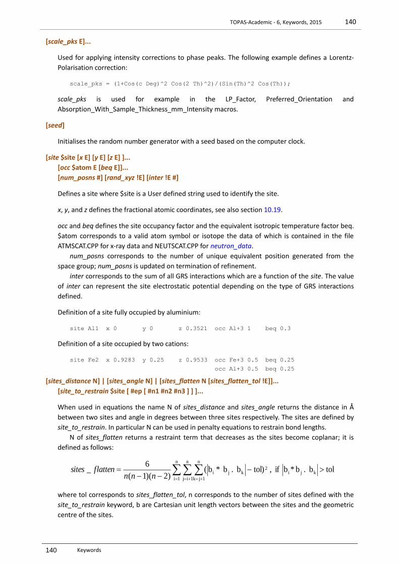
TOPAS-Academic - 6, Keywords, 2015 140
140 Keywords
[scale_pks E]...
Used for applying intensity corrections to phase peaks. The following example defines a Lorentz-
Polarisation correction:
scale_pks = (1+Cos(c Deg)^2 Cos(2 Th)^2)/(Sin(Th)^2 Cos(Th));
scale_pks is used for example in the LP_Factor, Preferred_Orientation and
Absorption_With_Sample_Thickness_mm_Intensity macros.
[seed]
Initialises the random number generator with a seed based on the computer clock.
[site $site [x E] [y E] [z E] ]...
[occ $atom E [beq E]]...
[num_posns #] [rand_xyz !E] [inter !E #]
Defines a site where $site is a User defined string used to identify the site.
x, y, and z defines the fractional atomic coordinates, see also section 10.19.
occ and beq defines the site occupancy factor and the equivalent isotropic temperature factor beq.
$atom corresponds to a valid atom symbol or isotope the data of which is contained in the file
ATMSCAT.CPP for x-ray data and NEUTSCAT.CPP for neutron_data.
num_posns corresponds to the number of unique equivalent position generated from the
space group; num_posns is updated on termination of refinement.
inter corresponds to the sum of all GRS interactions which are a function of the site. The value
of inter can represent the site electrostatic potential depending on the type of GRS interactions
defined.
Definition of a site fully occupied by aluminium:
site Al1 x 0 y 0 z 0.3521 occ Al+3 1 beq 0.3
Definition of a site occupied by two cations:
site Fe2 x 0.9283 y 0.25 z 0.9533 occ Fe+3 0.5 beq 0.25
occ Al+3 0.5 beq 0.25
[sites_distance N] | [sites_angle N] | [sites_flatten N [sites_flatten_tol !E]]...
[site_to_restrain $site [ #ep [ #n1 #n2 #n3 ] ] ]...
When used in equations the name N of sites_distance and sites_angle returns the distance in Å
between two sites and angle in degrees between three sites respectively. The sites are defined by
site_to_restrain. In particular N can be used in penalty equations to restrain bond lengths.
N of sites_flatten returns a restraint term that decreases as the sites become coplanar; it is
defined as follows:
n
1i
n
1ij
n
1jk
kji2
kji tol b . b *b if , tol) b . b * b()2)(1(
6_
nnnflattensites
where tol corresponds to sites_flatten_tol, n corresponds to the number of sites defined with the
site_to_restrain keyword, b are Cartesian unit length vectors between the sites and the geometric
centre of the sites.

TOPAS-Academic - 6, Keywords, 2015 141
141 Keywords
#eq, #n1, #n2 and #n3 correspond to the site equivalent position and fractional offsets to add
to the sites. This is useful if the structure is already known and constraints are required, for
example, in the bond length output (see append_bond_lengths):
Zr1:0 O1:20 0 0 -1 2.08772
O1:7 0 -1 0 2.08772 89.658
O1:10 0 0 -1 2.08772 90.342 90.342
O1:15 -1 0 0 2.08772 180.000 89.658 89.658
O1:18 -1 0 0 2.08772 90.342 89.658 180.000 90.342
P1:0 O1:4 0 0 0 1.52473
O1:8 0 0 0 1.52473 112.923
O1:0 0 0 0 1.52473 112.923 112.923
O2:0 0 0 0 1.59001 105.749 105.749 105.749
Example constraints using macros could look like the following:
Angle_Restrain(O1 P1 O1 8, 112, 112.92311, 0, 0.001)
Angle_Restrain(O1 18 -1 0 0 Zr1 O1 10 0 0 -1, 89, 89.65750, 0, 0.001)
Distance_Restrain(Zr1 O1 20 0 0 -1, 2.08, 2.08772, 0, 1)
BENZENE.INP demonstrates the use of the restraint macros Distance_Restrain, Angle_Restrain and
Flatten. OpenGL viewing is recommended. Note, for more than 6 sites then sites_flatten becomes
computationally expensive.
[sites_geometry $Name]...
[site_to_restrain $site [ #ep [ #n1 #n2 #n3 ] ] ]...
sites_geometry defines a grouping of up to four sites; $Name is the name given to ths grouping.
The sites that are part of the group is defined using site_to_restrain, for example:
sites_geometry some_name
load site_to_restrain { C1 C2 C3 C4 }
Three functions, Sites_Geometry_Distance($Name), Sites_Geometry_Angle($Name) and
Sites_Geometry_Dihedral_Angle($Name) can be used in equations to obtain the distance between
sites C1 and C2, the angle between C1-C2-C3 and the dihedral angle formed between the planes
C1-C2-C3 and C2-C3-C4. The convention used are the same as for z-matrices, see example
SITES_GEOMETRY_1.INP:
If $Name contains only two sites then only Sites_Geometry_Distance($Name) can be used.
Three sites defined additionally allows the use of Sites_Geometry_Angle($Name) and four sites
defined additionally allows the use of Sites_Geometry_Dihedral_Angle($Name).
Examples SITES_GEOMETRY_1.INP and SITES_GEOMETRY_2.INP demonstartes the use of
sites_geometry.
[siv_s1_s2 # #]
Defines the S1 and S2 integration limits for the spherical interaction volume of the GRS series.
[smooth #num_pts_left_right]
Performs a Savitzky-Golay smoothing on the observed data. The smoothing encompasses
(2 * #num_pts_left_right + 1) points.

TOPAS-Academic - 6, Keywords, 2015 142
142 Keywords
[spherical_harmonics_hkl $name]...
[sh_Cij_prm $Yij E]...
[sh_alpha !E]
[sh_order #]
Defines a hkl dependent symmetrized spherical harmonics series (see section 10.21.2). $name
defines the name given to the series and when used in equations it returns the value of the
spherical harmonics series.
sh_Cij_prm is the spherical harmonics coefficients, which can be defined by the User, or,
alternatively if there are no coefficients defined then the sh_Cij_prm parameters are generated.
Only the coefficients allowed by the selection rules of the point group are generated (Järvinen,
1993). At the end of refinement the generated sh_Cij_prm parameters are appended to sh_order.
This allows for control over the sh_Cij_prm parameters in subsequent refinements. $Yij
corresponds to valid symmetrized harmonics that has survived symmetrization. It is internally
generated when there are no sh_Cij_prm parameters defined by the User.
sh_alpha corresponds to the angle in degrees between the polar axis and the scattering
vector; sh_alpha defaults to zero degrees which is required for symmetric reflection as is the case
for Bragg-Brentano geometry.
sh_order corresponds to the order of the spherical harmonic series which are even numbers
ranging from 2 to 8 for non-cubic and from 2 to 10 for cubic systems.
The PO_Spherical_Harmonics macro simplifies the use of spherical_harmonics_hkl. CLAY.INP
demonstrates the use of spherical_harmonics_hkl for describing anisotropic peak shapes.
[stacked_hats_conv [whole_hat E [hat_height E]]...[half_hat E [hat_height E]...]...
Defines hat sizes for generating an aberration function comprising a summation of hat functions.
whole_hat defines a hat with an X axis extent of whole_hat/2. half_hat defines a hat with an X-
axis range of half_hat to zero if half_hat<0; or zero to half_hat if half_hat> 0. hat_height defines
the height of the hat; it defaults to 1. stacked_hats is used for example to describe tube tails using
the Tube_Tails macro.
[start_X !E] [finish_X !E]
Defines the start and finish X region to fit to.
[str | dummy_str]...
Defines a new structure node.
[str_hkl_angle N h k l]...
Defines a parameter name and a vector normal to the plane defined by h, k and l. When the
parameter name is used in an equation, it returns angles (in radians) between itself and the
normal to the planes defined by hkls; see the Preferred_Orientation and PO_Two_Directions
macros. An example in two directions is as follows:
[temperature !E]...
[move_to_the_next_temperature_regardless_of_the_change_in_rwp]
[save_values_as_best_after_randomization]
[use_best_values]
A temperature regime has no affect unless the reserved parameter name T is used in
val_on_continue attributes, or, if the following temperature dependent keywords are used:
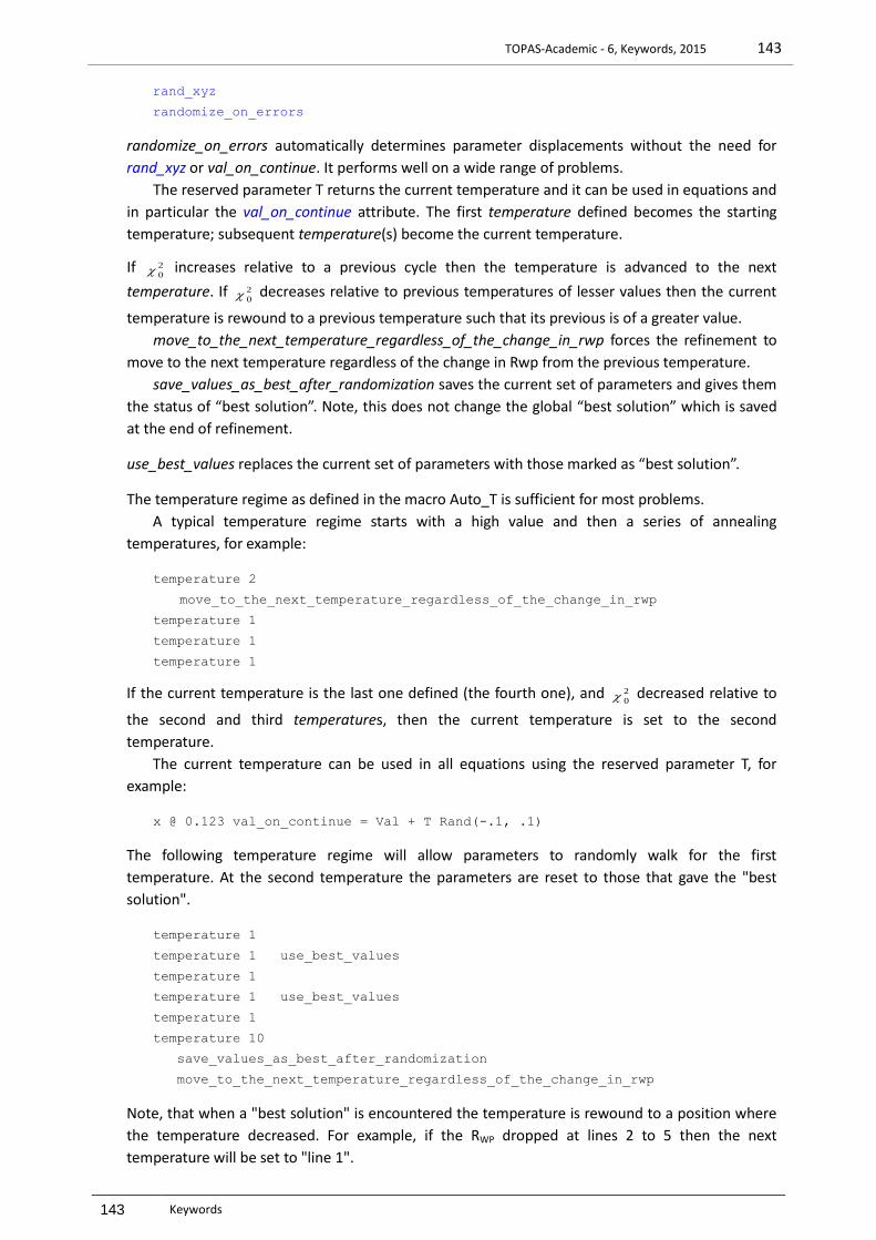
TOPAS-Academic - 6, Keywords, 2015 143
143 Keywords
rand_xyz
randomize_on_errors
randomize_on_errors automatically determines parameter displacements without the need for
rand_xyz or val_on_continue. It performs well on a wide range of problems.
The reserved parameter T returns the current temperature and it can be used in equations and
in particular the val_on_continue attribute. The first temperature defined becomes the starting
temperature; subsequent temperature(s) become the current temperature.
If 2
0 increases relative to a previous cycle then the temperature is advanced to the next
temperature. If 2
0 decreases relative to previous temperatures of lesser values then the current
temperature is rewound to a previous temperature such that its previous is of a greater value.
move_to_the_next_temperature_regardless_of_the_change_in_rwp forces the refinement to
move to the next temperature regardless of the change in Rwp from the previous temperature.
save_values_as_best_after_randomization saves the current set of parameters and gives them
the status of “best solution”. Note, this does not change the global “best solution” which is saved
at the end of refinement.
use_best_values replaces the current set of parameters with those marked as “best solution”.
The temperature regime as defined in the macro Auto_T is sufficient for most problems.
A typical temperature regime starts with a high value and then a series of annealing
temperatures, for example:
temperature 2
move_to_the_next_temperature_regardless_of_the_change_in_rwp
temperature 1
temperature 1
temperature 1
If the current temperature is the last one defined (the fourth one), and 2
0 decreased relative to
the second and third temperatures, then the current temperature is set to the second
temperature.
The current temperature can be used in all equations using the reserved parameter T, for
example:
x @ 0.123 val_on_continue = Val + T Rand(-.1, .1)
The following temperature regime will allow parameters to randomly walk for the first
temperature. At the second temperature the parameters are reset to those that gave the "best
solution".
temperature 1
temperature 1 use_best_values
temperature 1
temperature 1 use_best_values
temperature 1
temperature 10
save_values_as_best_after_randomization
move_to_the_next_temperature_regardless_of_the_change_in_rwp
Note, that when a "best solution" is encountered the temperature is rewound to a position where
the temperature decreased. For example, if the RWP dropped at lines 2 to 5 then the next
temperature will be set to "line 1".

TOPAS-Academic - 6, Keywords, 2015 144
144 Keywords
The following will continuously use the "best solution" before randomisation. This particular
temperature regime has a tendency to remain in a false minimum.
temperature 1 use_best_values
[th2_offset E]...
Used for applying 2 corrections to phase peaks. The following example applies a sample
displacement correction:
th2_offset = -2 Rad (c) Cos(Th) / Rs;
th2_offset is used for example in the Zero_Error and Specimen_Displacement macros.
[user_defined_convolution E min E max E]...
User defined convolutions are convoluted into phase peaks and can be a function of X. The
min/max equations are mandatory, they define the x-axis extents of the user_defined_convolution
where min <= 0 and max >= 0. For example, a sinc function can be convoluted into phase peaks
(example AU111.INP) as follows:
str
prm k 10 min 0.001 max 100
user_defined_convolution =
If(Abs(X) < 10^(-10), 1, (Sin(k X) /(k X))^2);
min -3 max 3
[use_tube_dispersion_coefficients]
Forces the use of Laboratory tube anomalous dispersion coefficients instead of the more accurate
data from http://www-cxro.lbl.gov/optical_constants/asf.html.
[verbose #]...
A value of 1 (the default) instructs the kernel to output in a verbose manner. A value of 0 reduces
kernel output such that text output is only initiated at the end of a refinement cycle. A value of -1
reduces kernel output such that text output is initiated every second and only Rwp values at the
end of a refinement cycle is kept. The Simulated_Annealing_1 macro has verbose set to -1; this
ensures that long simulated annealing runs do not exhaust memory due to saving Rwp values and
text output buffers.
[view_structure]
Informs a driver GUI to display the structure.
[weighting !E [recal_weighting_on_iter]]
Used for calculating the xdd dependent weighting function in 2
0 . Can be a function of the
reserved parameter names X, Yobs, Ycalc and SigmaYobs. The default is as follows:
weighting = 1 / Max(Yobs, 1);
In cases where weighting is a function of Ycalc then recal_weighting_on_iter can be used to
recalculate the weighting at the start of refinement iterations. Otherwise the weighting is
recalculated at the start of each refinement cycle.
Note that some goodness of fit indicators such as r_wp are a function of weighting, see Table 4-2.

TOPAS-Academic - 6, Keywords, 2015 145
145 Keywords
[weight_percent_amorphous !E]
Determines the amorphous content in a sample. The phase dependent keyword of
spiked_phase_measured_weight_percent needs to be defined in order for
weight_percent_amorphous to be calculated.
[x_calculation_step !E]
Calculation step used in the generation of phase peaks and fit_obj’s. Peak_Calculation_Step is the
actual step size used, it is defined is as follows:
For and x-axis with equal steps and x_calculation_step not defined then
Peak_Calculation_Step = “Observed data step size” / convolution_step
otherwise
Peak_Calculation_Step = x_calculation_step / convolution_step
x_calculation_step can be a function of Xo and Th. In some situations it may be computationally
efficient to write x_calculation_step in terms of the function Yobs_dx_at and the reserved
parameter Xo. It is also mandatory to define x_calculation_step for data with unequal x-axis steps
(*.xy or *.xye data files). Example uses of x_calculation_step is as follows:
x_calculation_step .01
x_calculation_step = .02 (1 + Tan(Th));
x_calculation_step = Yobs_dx_at(Xo);
[xdd $file [{ $data }] [range #] [xye_format] [gsas_format] [fullprof_format] ]...
Defines the start of xdd dependent keywords and the file containing the observed data.
{$data} allow for insertion of ASCII data directly into the INP file.
range applies to Bruker AXS *.RAW data files; in multi-range files it defines the range to be refined
with the first range starting at 1. range is set to 1 by default.
xye_format (see section 10.24 as well) signals the loading of columns of x, y and error values;
additional columns are ignored. gsas_format and fullprof_format signals the loading of GSAS and
FullProf file formats. The following instruction will refine on the first range in the data file
pbso4.raw:
xdd pbso4.raw
To following will refine on the third range:
xdd pbso4.raw range 3
To read data directly from an INP file, the following can be used:
xdd {
1 1 10 ' start, step and finish (equidistant data)
1 2 3 4 5 6 7 8 9 10
}
xdd {
_xy ' switch indicating x-y format
0.1 1 0.2 2 ...
}

TOPAS-Academic - 6, Keywords, 2015 146
146 Keywords
[xdd_out $file [append] ]...
Used for writing xdd dependent details to file. The out_eqn can contain the reserved parameter
names of X, Yobs, Ycalc and SigmaYobs. See the keyword out for a description of out_record. The
Out_Yobs_Ycalc_and_Difference macro is a good example of using xdd_out.
[xdd_scr $file] …
[dont_merge_equivalent_reflections]
[dont_merge_Friedel_pairs]
[ignore_differences_in_Friedel_pairs]
[str]…
[auto_scale !E]
[i_on_error_ratio_tolerance #]
[num_highest_I_values_to_keep #num]
xdd_scr defines single crystal data from the file $file. The file can have extensions of *.HKL for
ShelX HKL4 format or *.SCR for SCR format. All xdd and str keywords that are not dependent on
powder data can be used by xdd_scr. Single crystal data is internally stored in 2 versus Fo2 format.
This means that a lam definition is necessary and the keywords start_X, finish_X and exclude can
be used with xdd_scr.
dont_merge_equivalent_reflections unmerges equivalent reflections, see also section 10.2.3.
dont_merge_Friedel_pairs prevents the merging of Friedel pairs.
ignore_differences_in_Friedel_pairs forces the use of Eq. (10-12) for calculating F2.
auto_scale rewrites the scale parameter in terms of F2. This eliminates the need for the scale
parameter. The value determined for auto_scale is updated at the end of refinement.
i_on_error_ratio_tolerance filters out hkl’s that does not meet the condition:
|Fo| > i_on_error_ratio_tolerance |Sigma(Fo)|
num_highest_I_values_to_keep removes all hkl’s except for #num hkl’s with the highest Fo values.
An example input segment for single crystal data refinement is as follows:
xdd_scr ylidm.hkl
MoKa2(0.001)
finish_X 35
weighting = 1 / (Sin(X Deg / 2) Max(1, Yobs));
STR(P212121)
a 5.9636
b 9.0390
c 18.3955
scale @ 1.6039731906
i_on_error_ratio_tolerance 4
site S1 x @ 0.8090 y @ 0.1805 z @ 0.7402 occ S 1 beq 2
site O1 x @ 0.0901 y @ 0.8151 z @ 0.2234 occ O 1 beq 2
...
The SCR format is white space delimited and consists of entries of h, k, l, m, d, 2, Fo2 which is the
format outputted by the Create_hklm_d_Th2_Ip_file macro.
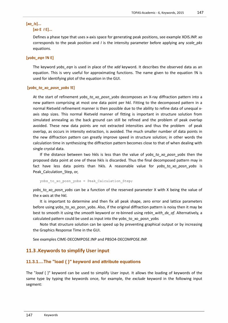
TOPAS-Academic - 6, Keywords, 2015 147
147 Keywords
[xo_Is]...
[xo E I E]...
Defines a phase type that uses x-axis space for generating peak positions, see example XOIS.INP. xo
corresponds to the peak position and I is the intensity parameter before applying any scale_pks
equations.
[yobs_eqn !N E]
The keyword yobs_eqn is used in place of the xdd keyword. It describes the observed data as an
equation. This is very useful for approximating functions. The name given to the equation !N is
used for identifying plot of the equation in the GUI.
[yobs_to_xo_posn_yobs !E]
At the start of refinement yobs_to_xo_posn_yobs decomposes an X-ray diffraction pattern into a
new pattern comprising at most one data point per hkl. Fitting to the decomposed pattern in a
normal Rietveld refinement manner is then possible due to the ability to refine data of unequal x-
axis step sizes. This normal Rietveld manner of fitting is important in structure solution from
simulated annealing as the back ground can still be refined and the problem of peak overlap
avoided. These new data points are not extracted intensities and thus the problem of peak
overlap, as occurs in intensity extraction, is avoided. The much smaller number of data points in
the new diffraction pattern can greatly improve speed in structure solution; in other words the
calculation time in synthesizing the diffraction pattern becomes close to that of when dealing with
single crystal data.
If the distance between two hkls is less than the value of yobs_to_xo_posn_yobs then the
proposed data point at one of these hkls is discarded. Thus the final decomposed pattern may in
fact have less data points than hkls. A reasonable value for yobs_to_xo_posn_yobs is
Peak_Calculation_Step, or,
yobs_to_xo_posn_yobs = Peak_Calculation_Step;
yobs_to_xo_posn_yobs can be a function of the reserved parameter X with X being the value of
the x-axis at the hkl.
It is important to determine and then fix all peak shape, zero error and lattice parameters
before using yobs_to_xo_posn_yobs. Also, if the original diffraction pattern is noisy then it may be
best to smooth it using the smooth keyword or re-binned using rebin_with_dx_of. Alternatively, a
calculated pattern could be used as input into the yobs_to_xo_posn_yobs
Note that structure solution can be speed up by preventing graphical output or by increasing
the Graphics Response Time in the GUI.
See examples CIME-DECOMPOSE.INP and PBSO4-DECOMPOSE.INP.
11.3 . Keywords to simplify User input
11.3.1 ....The "load { }" keyword and attribute equations
The "load { }" keyword can be used to simplify User input. It allows the loading of keywords of the
same type by typing the keywords once, for example, the exclude keyword in the following input
segment:
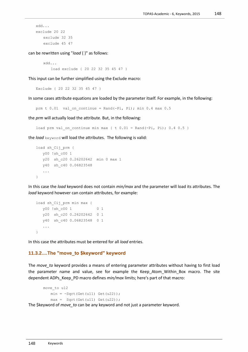
TOPAS-Academic - 6, Keywords, 2015 148
148 Keywords
xdd...
exclude 20 22
exclude 32 35
exclude 45 47
can be rewritten using "load { }" as follows:
xdd...
load exclude { 20 22 32 35 45 47 }
This input can be further simplified using the Exclude macro:
Exclude { 20 22 32 35 45 47 }
In some cases attribute equations are loaded by the parameter itself. For example, in the following:
prm t 0.01 val_on_continue = Rand(-Pi, Pi); min 0.4 max 0.5
the prm will actually load the attribute. But, in the following:
load prm val_on_continue min max { t 0.01 = Rand(-Pi, Pi); 0.4 0.5 }
the load keyword will load the attributes. The following is valid:
load sh_Cij_prm {
y00 !sh_c00 1
y20 sh_c20 0.26202642 min 0 max 1
y40 sh_c40 0.06823548
...
}
In this case the load keyword does not contain min/max and the parameter will load its attributes. The
load keyword however can contain attributes, for example:
load sh_Cij_prm min max {
y00 !sh_c00 1 0 1
y20 sh_c20 0.26202642 0 1
y40 sh_c40 0.06823548 0 1
...
}
In this case the attributes must be entered for all load entries.
11.3.2 ....The "move_to $keyword" keyword
The move_to keyword provides a means of entering parameter attributes without having to first load
the parameter name and value, see for example the Keep_Atom_Within_Box macro. The site
dependent ADPs_Keep_PD macro defines min/max limits; here's part of that macro:
move_to u12
min = -Sqrt(Get(u11) Get(u22));
max = Sqrt(Get(u11) Get(u22));
The $keyword of move_to can be any keyword and not just a parameter keyword.

TOPAS-Academic - 6, Keywords, 2015 149
149 Keywords
11.3.3 ....The "for xdds { }" and "for strs { }" constructs
The “for xdds { }” and "for strs { }" constructs simplify the construction of input files when there are
multiple diffraction patterns with similar structures, see example QUARTZ2_FPA.INP. For example, two
diffraction patterns with the same structures can be composed as follows:
xdd ... ‘ first xdd
bkg ...
th2_offset ...
...
‘ xdd dependent, not common to the xdd's
str... ‘ first str
scale ...
...
‘ str dependent, not common to the str's
xdd ... ‘ second xdd
bkg ...
th2_offset ...
...
‘ xdd dependent, not common to the xdd's
str... ‘ second str
scale ...
...
‘ str dependent, not common to the str's
for xdds {
Slit_Width(.2)
CuKa2
...
‘ xdd dependent, common to the xdd's
for strs { ‘ str dependent, common to the xdd's
...
}
for strs 1 to 1 {
space_group p1
site ...
‘ str dependent, specific to the first str
}
}
For obvious reasons, parameters should not be given the @ name within for constructs. The effect this
would have is to give unique parameter names to the parameters iterated over; the output file would
contain the parameter value corresponding to the last “for xdds” or “for strs” iteration.
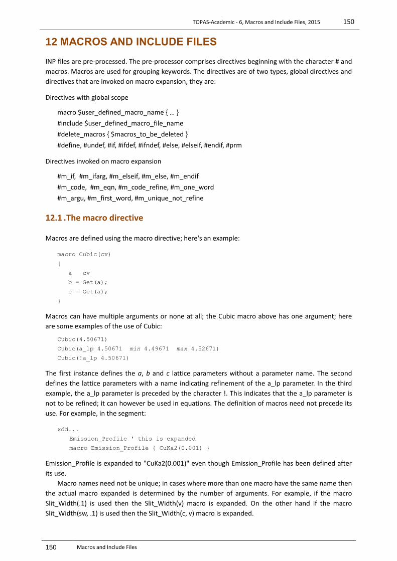
TOPAS-Academic - 6, Macros and Include Files, 2015 150
150 Macros and Include Files
12 MACROS AND INCLUDE FILES
INP files are pre-processed. The pre-processor comprises directives beginning with the character # and
macros. Macros are used for grouping keywords. The directives are of two types, global directives and
directives that are invoked on macro expansion, they are:
Directives with global scope
macro $user_defined_macro_name { … }
#include $user_defined_macro_file_name
#delete_macros { $macros_to_be_deleted }
#define, #undef, #if, #ifdef, #ifndef, #else, #elseif, #endif, #prm
Directives invoked on macro expansion
#m_if, #m_ifarg, #m_elseif, #m_else, #m_endif
#m_code, #m_eqn, #m_code_refine, #m_one_word
#m_argu, #m_first_word, #m_unique_not_refine
12.1 . The macro directive
Macros are defined using the macro directive; here's an example:
macro Cubic(cv)
{
a cv
b = Get(a);
c = Get(a);
}
Macros can have multiple arguments or none at all; the Cubic macro above has one argument; here
are some examples of the use of Cubic:
Cubic(4.50671)
Cubic(a_lp 4.50671 min 4.49671 max 4.52671)
Cubic(!a_lp 4.50671)
The first instance defines the a, b and c lattice parameters without a parameter name. The second
defines the lattice parameters with a name indicating refinement of the a_lp parameter. In the third
example, the a_lp parameter is preceded by the character !. This indicates that the a_lp parameter is
not to be refined; it can however be used in equations. The definition of macros need not precede its
use. For example, in the segment:
xdd...
Emission_Profile ' this is expanded
macro Emission_Profile { CuKa2(0.001) }
Emission_Profile is expanded to "CuKa2(0.001)" even though Emission_Profile has been defined after
its use.
Macro names need not be unique; in cases where more than one macro have the same name then
the actual macro expanded is determined by the number of arguments. For example, if the macro
Slit_Width(.1) is used then the Slit_Width(v) macro is expanded. On the other hand if the macro
Slit_Width(sw, .1) is used then the Slit_Width(c, v) macro is expanded.

TOPAS-Academic - 6, Macros and Include Files, 2015 151
151 Macros and Include Files
Macros can also expand to other macro names. For example, the macro Crystallite_Size expands to
CS and since CS is a macro then the CS macro will be expanded.
12.1.1 ....Directives with global scope
#include $user_defined_macro_file_name
Include files are used to group macros. The file TOPAS.INC contains standard macros; a good place to
view examples. Text within include files are inserted at the position of the #include directive, thus the
following:
#include "my include file.inc"
inserts the text within "my include file.inc" at the position of the #include directive. The standard
macro file TOPAS.INC is always included by default.
#delete_macros { $macros_to_be_deleted }
Macros can be deleted using the #delete_macros keyword, for example,
#delete_macros { LP_Factor SW ZE }
will delete all macros previously defined with the names LP_Factor, SW and ZE including macros of the
same name but with different arguments.
#define, #undef, #ifdef, #ifndef, #else, #endif
The #define and #undef directives works similar to the c pre-processor directives of the same name.
#define and #undef is typically used with #ifdef, #else, #endif directives to control macro expansion in
INP files. For example, the following:
#ifdef STANDARD_MACROS
xdd...
#endif
will expand to contain the xdd keyword if STANDARD_MACROS has been previously defined using a
#define directive. The following will also expand to contain the xdd keyword if STANDARD_MACROS
has not been defined using a #define directive,
#ifdef !STANDARD_MACROS
#define STANDARD_MACROS
xdd...
#endif
or,
#ifndef STANDARD_MACROS
#define STANDARD_MACROS
xdd...
#endif
Note the use of the ‘!’ character placed before STANDARD_MACROS which means if
STANDARD_MACROS is not defined.
12.1.2 ....Pre-processor equations and #prm, #if, #elseif, #out
Pre-processor parameters, called hash parameters, can be defined by placing a # before the text prm.
#prm’s can be a function of other #prm’s and they can be used in #if, #elseif, #m_if and #m_elseif pre-

TOPAS-Academic - 6, Macros and Include Files, 2015 152
152 Macros and Include Files
processor statements. #prm’s are only evaluated at the pre-processor stage of loading INP files (see
test_examples\hash_prm.inp); they are therefore unknown to the kernel and are totally separate to
parameters defined using prm. Pre-processed output can be found in the TOPAS.LOG file when
running TA.EXE or TC.LOG when running TC.EXE.
The #out and #m_out allows pre-processor #prm’s values, which can be strings or numbers, to be
placed into the pre-processed text. For example:
#prm a = Constant(Rand(0,1));
#out a
will output a random number between 0 and 1 into the pre-processed file at the position of #out. INP
files can therefore be manipulated with #prm’s and #if statements with a means of identifying the
manipulation carried out.
The following:
macro Ex1(a)
{
#m_if a == "b";
Yes b
#m_elseif a == “c”;
Yes c
#m_endif
}
Ex1("b")
expands to:
Yes b
In the following:
#prm ran = Constant(Rand(0,1));
#if ran < 0.5;
view_structure
#endif
#if ran < 0.5;
view_structure
#endif
#if ran < 0.5;
view_structure
#endif
each call to ‘ran’ in the #if statements would return the same value because of the use of Constant.
More complicated INP file manipulation is shown in the following:
#prm space_group_number = 4;
#if And(space_group_number >= 75, space_group_number <= 142);
...
#elseif And(space_group_number >= 16, space_group_number <= 74);
...
#endif
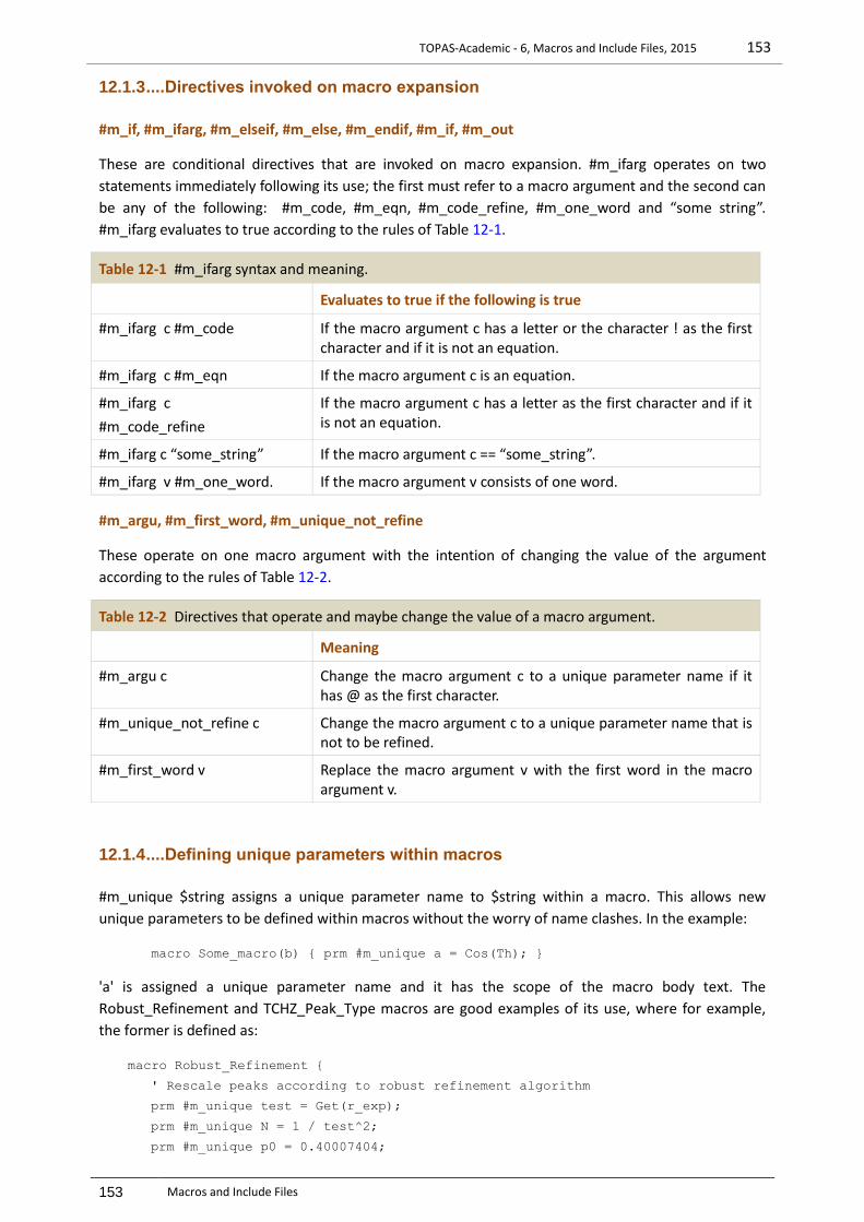
TOPAS-Academic - 6, Macros and Include Files, 2015 153
153 Macros and Include Files
12.1.3 ....Directives invoked on macro expansion
#m_if, #m_ifarg, #m_elseif, #m_else, #m_endif, #m_if, #m_out
These are conditional directives that are invoked on macro expansion. #m_ifarg operates on two
statements immediately following its use; the first must refer to a macro argument and the second can
be any of the following: #m_code, #m_eqn, #m_code_refine, #m_one_word and “some string”.
#m_ifarg evaluates to true according to the rules of Table 12-1.
Table 12-1 #m_ifarg syntax and meaning.
Evaluates to true if the following is true
#m_ifarg c #m_code If the macro argument c has a letter or the character ! as the first character and if it is not an equation.
#m_ifarg c #m_eqn If the macro argument c is an equation.
#m_ifarg c
#m_code_refine
If the macro argument c has a letter as the first character and if it is not an equation.
#m_ifarg c “some_string” If the macro argument c == “some_string”.
#m_ifarg v #m_one_word. If the macro argument v consists of one word.
#m_argu, #m_first_word, #m_unique_not_refine
These operate on one macro argument with the intention of changing the value of the argument
according to the rules of Table 12-2.
Table 12-2 Directives that operate and maybe change the value of a macro argument.
Meaning
#m_argu c Change the macro argument c to a unique parameter name if it has @ as the first character.
#m_unique_not_refine c Change the macro argument c to a unique parameter name that is not to be refined.
#m_first_word v Replace the macro argument v with the first word in the macro argument v.
12.1.4 ....Defining unique parameters within macros
#m_unique $string assigns a unique parameter name to $string within a macro. This allows new
unique parameters to be defined within macros without the worry of name clashes. In the example:
macro Some_macro(b) { prm #m_unique a = Cos(Th); }
'a' is assigned a unique parameter name and it has the scope of the macro body text. The
Robust_Refinement and TCHZ_Peak_Type macros are good examples of its use, where for example,
the former is defined as:
macro Robust_Refinement {
' Rescale peaks according to robust refinement algorithm
prm #m_unique test = Get(r_exp);
prm #m_unique N = 1 / test^2;
prm #m_unique p0 = 0.40007404;

TOPAS-Academic - 6, Macros and Include Files, 2015 154
154 Macros and Include Files
prm #m_unique p1 = -2.5949286;
prm #m_unique p2 = 4.3513542;
prm #m_unique p3 = -1.7400101;
prm #m_unique p4 = 3.6140845e-1;
prm #m_unique p5 = -4.45247609e-2;
prm #m_unique p6 = 3.5986364e-3;
prm #m_unique p7 = -1.8328008e-4;
prm #m_unique p8 = 5.7937184e-6;
prm #m_unique p9 = -1.035303e-7;
prm #m_unique p10 = 7.9903166e-10;
prm #m_unique t = (Yobs - Ycalc) / SigmaYobs;
weighting = If( t < 0.8,
N / Max(SigmaYobs^2, 1),
If( t < 21, N ((((((((((p10 t + p9) t + p8) t + p7)
t + p6) t + p5) t + p4) t + p3)
t + p2) t + p1) t + p0) / (Yobs - Ycalc)^2,
N (2.0131 Ln(t) + 3.9183) / (Yobs - Ycalc)^2));
recal_weighting_on_iter
}
12.1.5 ....Superfluous parentheses and the '&' Type for macros and its arguments
The pre-processor is an un-typed language meaning that it knows nothing about the type of text
passed to macro arguments. This has great flexibility but there can be drawbacks; for example, the
following:
macro divide(a, b) { a / b }
prm e = divide(a+b, c-d);
expands to the unintended result of:
prm e = a + b / c - d;
The writer of the macro could solve this problem by rewriting the macro with parentheses:
macro divide(a, b) { (a) /( b) }
Alternatively the & Type can be used for macros that expect equation type arguments. Defining the
macro with '&' before the arguments as in:
macro divide(& a, & b) { a / b }
prm e = divide(a+b, c-d);
instructs the pre-processor that the argument is of an equation Type and a check is made to
determine whether the argument needs parentheses. This results in the correct expansion of:
prm e = (a+b) / (c-d);
Even with & types used for arguments, the following:
macro divide(& a, & b) { a / b }
prm e = divide(a+b, c-d)^2;
expands to the unintended:
prm e = (a + b) / (c - d)^2;

TOPAS-Academic - 6, Macros and Include Files, 2015 155
155 Macros and Include Files
The writer of the macro could again rewrite the macro to include more parentheses:
macro divide(a, b) { ((a) / (b)) }
Or, define the expansion of the macro itself to have an & Type by placing the & character before the
macro name itself as follows:
macro & divide(& a, & b) { a / b }
Expansion of prm e = divide(a+b, c-d)^2 now becomes the intended:
prm e = ((a + b) / (c - d))^2;
With the use of the & Type, macros such as Ramp defined in Version 4 as:
macro Ramp(x1, x2, n)
{
((x1) + ((x2)-(x1)) Mod(Cycle_Iter, (n)) / ((n)-1))
}
can now be written with less parentheses as follows:
macro & Ramp(& x1,& x2,& n) {
x1 + (x2-x1) Mod(Cycle_Iter, n) / (n-1)
}
12.2 . Overview
The file TOPAS.INC is included into INP files by default; it contains commonly used standard macros.
The meaning of the macro arguments in TOPAS.INC can be readily determined from the following
conventions:
Arguments called "c" correspond to a parameter name.
Arguments called "v" correspond to a parameter value.
Arguments called "cv" correspond to a parameter name and/or value.
For example, the macro Cubic(cv) requires a value and/or a parameter name as an argument. Some
examples are:
Cubic(a_lp 10.604)
Cubic(10.604)
Cubic(@ 10.604 min 10.59 max 10.61)
Here are some more examples for the Slit_Width macro:
SW(@, .1)
SW(sw, .1 min = Val-.02; max = Val+.02;)
SW((ap+bp)/cp, 0) ' where ap, bp anc cp are parameters defined elsewhere
12.2.1 ....xdd macros
RAW(path_no_ext)
RAW(path_no_ext, range_num)
DAT(path_no_ext)
XDD(path_no_ext)
XY(path_no_ext, calc_step)
XYE(path_ext)

TOPAS-Academic - 6, Macros and Include Files, 2015 156
156 Macros and Include Files
SCR(path_no_ext)
SHELX_HKL4(path_no_ext)
12.2.2 ....Lattice parameters
Cubic(cv)
Tetragonal(a_cv, c_cv)
Hexagonal(a_cv, c_cv)
Rhombohedral(a_cv, al_cv)
12.2.3 ....Emission profile macros
No_Th_Dependence
CuKa1(yminymax)
CuK1sharp(yminymax)
CuKa2_analyt(yminymax)
CuKa2(yminymax)
CuKa4_Holzer(yminymax)
CuKa5(yminymax)
CuKa5_Berger(yminymax)
CoKa3(yminymax)
CoKa7_Holzer(yminymax)
CrKa7_Holzer(yminymax)
FeKa7_Holzer(yminymax)
MnKa7_Holzer(yminymax)
NiKa5_Holzer(yminymax)
MoKa2(yminymax)
CuKb4_Holzer(yminymax)
CoKb6_Holzer(yminymax)
CrKb5_Holzer(yminymax)
FeKb4_Holzer(yminymax)
MnKb5_Holzer(yminymax)
NiKb4_Holzer(yminymax)
12.2.4 ....Instrument and instrument convolutions
Radius(rp, rs)
Primary and secondary instrument radii in [mm]. For most diffractometers rp equals rs.
Specimen_Tilt(c, v)
Specimen tilt in mm.
Slit_Width(c, v) or SW(c, v)
Aperture of the receiving slit in the equitorial plane in mm.
Sample_Thickness(dc, dv)
Sample thickness in mm in the direction of the scattering vector.
Divergence(c, v)
Horizontal divergence of the beam in degrees in the equitorial plane.
Variable_Divergence(c, v)
Variable_Divergence_Shape(c, v)
Variable_Divergence_Intensity
Constant illuminated sample length in mm for variable slits (i.e. variable beam divergence). This
Variable_Divergence macro applies both a shape and intensity correction.
Simple_Axial_Model(c, v)
Receiving slit length mm for describing peak asymmetry due to axial divergence.
Full_Axial_Model(filament_cv, sample_cv, detector_cv, psol_cv, ssol_cv)
Accurate model for describing peak asymmetry due to axial divergence of the beam.
[filament_cv]: Tube filament length in [mm].
[sample_cv]: Sample length in axial direction in [mm].
[detector_cv]: Length of the detector (= receiving) slit in [mm].
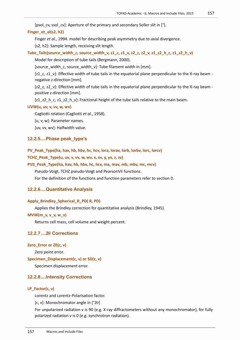
TOPAS-Academic - 6, Macros and Include Files, 2015 157
157 Macros and Include Files
[psol_cv, ssol_cv]: Aperture of the primary and secondary Soller slit in [°].
Finger_et_al(s2, h2)
Finger et al., 1994. model for describing peak asymmetry due to axial divergence.
[s2, h2]: Sample length, receiving slit length.
Tube_Tails(source_width_c, source_width_v, z1_c, z1_v, z2_c, z2_v, z1_z2_h_c, z1_z2_h_v)
Model for description of tube tails (Bergmann, 2000).
[source_width_c, source_width_v]: Tube filament width in [mm].
[z1_c, z1_v]: Effective width of tube tails in the equatorial plane perpendicular to the X-ray beam -
negative z-direction [mm].
[z2_c, z2_v]: Effective width of tube tails in the equatorial plane perpendicular to the X-ray beam -
positive z-direction [mm].
[z1_z2_h_c, z1_z2_h_v]: Fractional height of the tube tails relative to the main beam.
UVW(u, uv, v, vv, w, wv)
Cagliotti relation (Cagliotti et al., 1958).
[u, v, w]: Parameter names.
[uv, vv, wv]: Halfwidth value.
12.2.5 ....Phase peak_type's
PV_Peak_Type(ha, hav, hb, hbv, hc, hcv, lora, lorav, lorb, lorbv, lorc, lorcv)
TCHZ_Peak_Type(u, uv, v, vv, w, wv, x, xv, y, yv, z, zv)
PVII_Peak_Type(ha, hav, hb, hbv, hc, hcv, ma, mav, mb, mbv, mc, mcv)
Pseudo-Voigt, TCHZ pseudo-Voigt and PearsonVII functions.
For the definition of the functions and function parameters refer to section 0.
12.2.6 ....Quantitative Analysis
Apply_Brindley_Spherical_R_PD( R, PD)
Applies the Brindley correction for quantitative analysis (Brindley, 1945).
MVW(m_v, v_v, w_v)
Returns cell mass, cell volume and weight percent.
12.2.7 ....2 Corrections
Zero_Error or ZE(c, v)
Zero point error.
Specimen_Displacement(c, v) or SD(c, v)
Specimen displacement error.
12.2.8 ....Intensity Corrections
LP_Factor(c, v)
Lorentz and Lorentz-Polarisation factor.
[c, v]: Monochromator angle in [°2]
For unpolarized radiation v is 90 (e.g. X-ray diffractometers without any monochromator), for fully
polarized radiation v is 0 (e.g. synchrotron radiation).
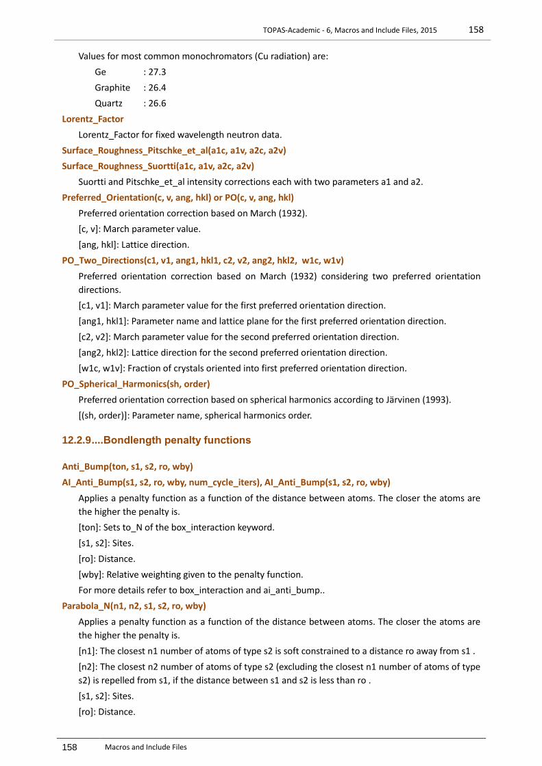
TOPAS-Academic - 6, Macros and Include Files, 2015 158
158 Macros and Include Files
Values for most common monochromators (Cu radiation) are:
Ge : 27.3
Graphite : 26.4
Quartz : 26.6
Lorentz_Factor
Lorentz_Factor for fixed wavelength neutron data.
Surface_Roughness_Pitschke_et_al(a1c, a1v, a2c, a2v)
Surface_Roughness_Suortti(a1c, a1v, a2c, a2v)
Suortti and Pitschke_et_al intensity corrections each with two parameters a1 and a2.
Preferred_Orientation(c, v, ang, hkl) or PO(c, v, ang, hkl)
Preferred orientation correction based on March (1932).
[c, v]: March parameter value.
[ang, hkl]: Lattice direction.
PO_Two_Directions(c1, v1, ang1, hkl1, c2, v2, ang2, hkl2, w1c, w1v)
Preferred orientation correction based on March (1932) considering two preferred orientation
directions.
[c1, v1]: March parameter value for the first preferred orientation direction.
[ang1, hkl1]: Parameter name and lattice plane for the first preferred orientation direction.
[c2, v2]: March parameter value for the second preferred orientation direction.
[ang2, hkl2]: Lattice direction for the second preferred orientation direction.
[w1c, w1v]: Fraction of crystals oriented into first preferred orientation direction.
PO_Spherical_Harmonics(sh, order)
Preferred orientation correction based on spherical harmonics according to Järvinen (1993).
[(sh, order)]: Parameter name, spherical harmonics order.
12.2.9 ....Bondlength penalty functions
Anti_Bump(ton, s1, s2, ro, wby)
AI_Anti_Bump(s1, s2, ro, wby, num_cycle_iters), AI_Anti_Bump(s1, s2, ro, wby)
Applies a penalty function as a function of the distance between atoms. The closer the atoms are
the higher the penalty is.
[ton]: Sets to_N of the box_interaction keyword.
[s1, s2]: Sites.
[ro]: Distance.
[wby]: Relative weighting given to the penalty function.
For more details refer to box_interaction and ai_anti_bump..
Parabola_N(n1, n2, s1, s2, ro, wby)
Applies a penalty function as a function of the distance between atoms. The closer the atoms are
the higher the penalty is.
[n1]: The closest n1 number of atoms of type s2 is soft constrained to a distance ro away from s1 .
[n2]: The closest n2 number of atoms of type s2 (excluding the closest n1 number of atoms of type
s2) is repelled from s1, if the distance between s1 and s2 is less than ro .
[s1, s2]: Sites.
[ro]: Distance.

TOPAS-Academic - 6, Macros and Include Files, 2015 159
159 Macros and Include Files
[wby]: Relative weighting given to the penalty function.
Grs_Interaction(s1, s2, wqi, wqj, c, ro, n)
Penalty function applying the GRS series according to Coelho & Cheary (1997).
[s1, s2]: Sites.
[wqi, wqj]: Valence charge of the atoms.
[c]: Name of the GRS.
[ro]: Distance.
[n]: The exponent of the repulsion part of the Lennard-Jones potential.
For more details refer to grs_interaction.
Grs_No_Repulsion(s1, s2, wqi, wqj, c)
Used for calculating the Madelung constants.
[s1, s2]: Sites.
[wqi, wqj]: Valence charge of the atoms.
[c]: Name of the GRS.
Grs_BornMayer(s1, s2, wqi, wqj, c, ro, b)
Uses the GRS series with a Born-Mayer equation for the repulsion term.
[s1, s2]: Sites.
[wqi, wqj]: Valence charge of the atoms.
[c]: Name of the GRS.
[ro]: Mean distance.
[b]: b-constant for the repulsion part of the Born-Mayer potential.
Distance_Restrain(sites, t, t_calc, tol, wscale)
Angle_Restrain(sites, t, t_calc, tol, wscale)
Flatten(sites, t_calc, tol, wscale)
Distance_Restrain_Keep_Within(sites, r, wby, num_cycle_iters)
Distance_Restrain_Keep_Out(sites, r, wby, num_cycle_iters)
Applies penalties restraining distances and angles between sites. .
'sites' must comprise two sites for the distance restraints and three for the angle restraints.. For
Flatten 'sites' must contain more than three sites. wby is a scaling constant applied to the penalty.
Keep_Atom_Within_Box(size) - this is a constraint macro.
Applies constraints such that the present site cannot more outside of a box with a length of 2*size.
12.2.10 ..Reporting macros
Create_2Th_Ip_file(file)
Creates a file with positions (2 ) and intensities.
Create_d_Ip_file(file)
Creates a file with positions (d) and intensities.
Create_hklm_d_Th2_Ip_file(file)
Creates a file with the following information for each peak: h, k, l, multiplicity, positions d and 2
and intensities.
Out_Yobs_Ycalc_and_Difference(file)
Outputs the x-axis, Yobs, Ycalc and difference.
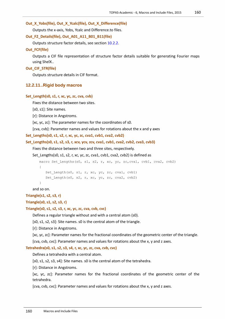
TOPAS-Academic - 6, Macros and Include Files, 2015 160
160 Macros and Include Files
Out_X_Yobs(file), Out_X_Ycalc(file), Out_X_Difference(file)
Outputs the x-axis, Yobs, Ycalc and Difference.to files.
Out_F2_Details(file), Out_A01_A11_B01_B11(file)
Outputs structure factor details, see section 10.2.2.
Out_FCF(file)
Outputs a CIF file representation of structure factor details suitable for generating Fourier maps
using ShelX..
Out_CIF_STR(file)
Outputs structure details in CIF format.
12.2.11 ..Rigid body macros
Set_Length(s0, s1, r, xc, yc, zc, cva, cvb)
Fixes the distance between two sites.
[s0, s1]: Site names.
[r]: Distance in Angstroms.
[xc, yc, zc]: The parameter names for the coordinates of s0.
[cva, cvb]: Parameter names and values for rotations about the x and y axes
Set_Lengths(s0, s1, s2, r, xc, yc, zc, cva1, cvb1, cva2, cvb2)
Set_Lengths(s0, s1, s2, s3, r, xcv, ycv, zcv, cva1, cvb1, cva2, cvb2, cva3, cvb3)
Fixes the distance between two and three sites, respectively.
Set_Lengths(s0, s1, s2, r, xc, yc, zc, cva1, cvb1, cva2, cvb2) is defined as
macro Set_Lengths(s0, s1, s2, r, xc, yc, zc,cva1, cvb1, cva2, cvb2)
{
Set_Length(s0, s1, r, xc, yc, zc, cva1, cvb1)
Set_Length(s0, s2, r, xc, yc, zc, cva2, cvb2)
}
and so on.
Triangle(s1, s2, s3, r)
Triangle(s0, s1, s2, s3, r)
Triangle(s0, s1, s2, s3, r, xc, yc, zc, cva, cvb, cvc)
Defines a regular triangle without and with a central atom (s0).
[s0, s1, s2, s3]: Site names. s0 is the central atom of the triangle.
[r]: Distance in Angstroms.
[xc, yc, zc]: Parameter names for the fractional coordinates of the geometric center of the triangle.
[cva, cvb, cvc]: Parameter names and values for rotations about the x, y and z axes.
Tetrahedra(s0, s1, s2, s3, s4, r, xc, yc, zc, cva, cvb, cvc)
Defines a tetrahedra with a central atom.
[s0, s1, s2, s3, s4]: Site names. s0 is the central atom of the tetrahedra.
[r]: Distance in Angstroms.
[xc, yc, zc]: Parameter names for the fractional coordinates of the geometric center of the
tetrahedra.
[cva, cvb, cvc]: Parameter names and values for rotations about the x, y and z axes.
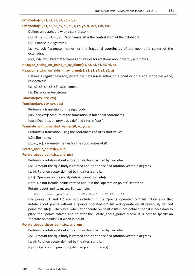
TOPAS-Academic - 6, Macros and Include Files, 2015 161
161 Macros and Include Files
Octahedra(s0, s1, s2, s3, s4, s5, s6, r)
Octahedra(s0, s1, s2, s3, s4, s5, s6, r, xc, yc, zc, cva, cvb, cvc)
Defines an octahedra with a central atom.
[s0, s1, s2, s3, s4, s5, s6]: Site names. s0 is the central atom of the octahedra.
[r]: Distance in Angstroms.
[xc, yc, zc]: Parameter names for the fractional coordinates of the geometric center of the
octahedra.
[cva, cvb, cvc]: Parameter names and values for rotations about the x, y and z axes.
Hexagon_sitting_on_point_in_xy_plane(s1, s2, s3, s4, s5, s6, a)
Hexagon_sitting_on_side_in_xy_plane(s1, s2, s3, s4, s5, s6, a)
Defines a regular hexagon, where the hexagon is sitting on a point or on a side in the x-y plane,
respectively.
[s1, s2, s3, s4, s5, s6]: Site names.
[a]: Distance in Angstroms.
Translate(acv, bcv, ccv)
Translate(acv, bcv, ccv, ops)
Performs a translation of the rigid body.
[acv, bcv, ccv]: Amount of the translation in fractional coordinates.
[ops]: Operates on previously defined sites in “ops”.
Translate_with_site_start_values(s0, xc, yc, zc)
Performs a translation using the coordinates of s0 as start values.
[s0]: Site name.
[xc, yc, zc]: Parameter names for the coordinates of s0.
Rotate_about_points(cv, a, b)
Rotate_about_points(cv, a, b, pts)
Performs a rotation about a rotation vector specified by two sites.
[cv]: Amount the rigid body is rotated about the specified rotation vector in degrees.
[a, b]: Rotation vector defined by the sites a and b.
[pts]: Operates on previously defined point_for_site(s).
Note: Do not include points rotated about in the “operate on points” list of the
Rotate_about_points macro. For example, in
Rotate_about_points(@ 1 0, C1, C2, " C3 C4 C5 C6 ")
the points C1 and C2 are not included in the “points operated on” list. Note also that
Rotate_about_points without a “points operated on” list will operate on all previously defined
point_for_site(s). Therefore, when an “operate on points” list is not defined then it is necessary to
place the “points rotated about” after the Rotate_about_points macro. It is best to specify an
“operate on points” list when in doubt.
Rotate_about_these_points(cv, a, b, ops)
Performs a rotation about a rotation vector specified by two sites.
[cv]: Amount the rigid body is rotated about the specified rotation vector in degrees.
[a, b]: Rotation vector defined by the sites a and b.
[ops]: Operates on previously defined point_for_site(s).
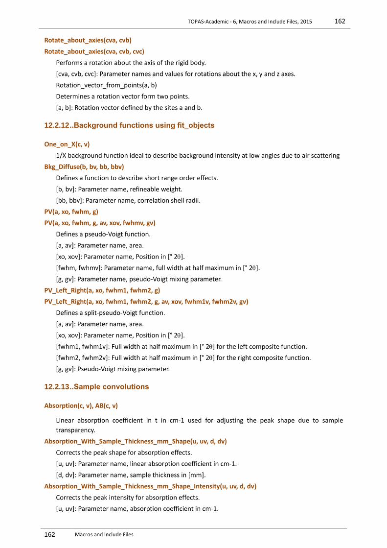
TOPAS-Academic - 6, Macros and Include Files, 2015 162
162 Macros and Include Files
Rotate_about_axies(cva, cvb)
Rotate_about_axies(cva, cvb, cvc)
Performs a rotation about the axis of the rigid body.
[cva, cvb, cvc]: Parameter names and values for rotations about the x, y and z axes.
Rotation_vector_from_points(a, b)
Determines a rotation vector form two points.
[a, b]: Rotation vector defined by the sites a and b.
12.2.12 ..Background functions using fit_objects
One_on_X(c, v)
1/X background function ideal to describe background intensity at low angles due to air scattering
Bkg_Diffuse(b, bv, bb, bbv)
Defines a function to describe short range order effects.
[b, bv]: Parameter name, refineable weight.
[bb, bbv]: Parameter name, correlation shell radii.
PV(a, xo, fwhm, g)
PV(a, xo, fwhm, g, av, xov, fwhmv, gv)
Defines a pseudo-Voigt function.
[a, av]: Parameter name, area.
[xo, xov]: Parameter name, Position in [° 2].
[fwhm, fwhmv]: Parameter name, full width at half maximum in [° 2].
[g, gv]: Parameter name, pseudo-Voigt mixing parameter.
PV_Left_Right(a, xo, fwhm1, fwhm2, g)
PV_Left_Right(a, xo, fwhm1, fwhm2, g, av, xov, fwhm1v, fwhm2v, gv)
Defines a split-pseudo-Voigt function.
[a, av]: Parameter name, area.
[xo, xov]: Parameter name, Position in [° 2].
[fwhm1, fwhm1v]: Full width at half maximum in [° 2] for the left composite function.
[fwhm2, fwhm2v]: Full width at half maximum in [° 2] for the right composite function.
[g, gv]: Pseudo-Voigt mixing parameter.
12.2.13 ..Sample convolutions
Absorption(c, v), AB(c, v)
Linear absorption coefficient in t in cm-1 used for adjusting the peak shape due to sample
transparency.
Absorption_With_Sample_Thickness_mm_Shape(u, uv, d, dv)
Corrects the peak shape for absorption effects.
[u, uv]: Parameter name, linear absorption coefficient in cm-1.
[d, dv]: Parameter name, sample thickness in [mm].
Absorption_With_Sample_Thickness_mm_Shape_Intensity(u, uv, d, dv)
Corrects the peak intensity for absorption effects.
[u, uv]: Parameter name, absorption coefficient in cm-1.

TOPAS-Academic - 6, Macros and Include Files, 2015 163
163 Macros and Include Files
[d, dv]: Parameter name, sample thickness in [mm].
CS_L(c,v) or Crystallite_Size(c, v) or CS(c, v)
Applies a Lorentzian convolution with a FWHM that varies according to the relation lor_fwhm = 0.1
Rad Lam / (c Cos(Th)).
[c, v]: Parameter name, crystallite size in [nm].
CS_G(c, v)
Applies a Gaussian convolution with a FWHM that varies according to the relation gauss_fwhm
=0.1 Rad Lam / (c Cos(Th)).
[c, v]: Parameter name, crystallite size in [nm].
Strain_L(c, v) or Microstrain(c, v) or MS(c, v)
Applies a Lorentzian convolution with a FWHM that varies according to the relation lor_fwhm = c
Tan(Th).
Strain_G(c, v)
Applies a Gaussian convolution with a FWHM that varies according to the relation gauss_fwhm = c
Tan(Th).
LVol_FWHM_CS_G_L(k, lvol, kf, lvolf, csgc, csgv, cslc, cslv)
Calculates FWHM and IB (integral breadth) based volume-weighted column heights (LVol). For
details refer to section 10.6.
[k, lvol]: shape factor (fixed to 1), integral breadth based LVol.
[kf, lvolf]: shape factor (defaults to 0.89), FWHM based LVol.
[csgc, csgv]: Parameter name, Gaussian component.
[cslc, cslv]: Parameter name, Lorentzian component.
12.2.14 ..Neutron TOF
TOF_XYE(path, calc_step), TOF_GSAS(path, calc_step)
Includes the neutron_data keyword and the calculation step size.
TOF_LAM(w_ymin_on_ymax)
Defines a simple emission profile suitable for TOF data
TOF_x_axis_calibration(t0, t0v, t1, t1v, t2, t2v)
Writes the pk_xo equation in terms of the three calibration constants t0, t1, t2 converting d-
spacing to x-axis space.
TOF_Exponential(a0, a0v, a1, a1v, wexp, t1, lr)
An exponential convolution applied to the TOF peaks - see example TOF_BANK2_1.INP.
TOF_CS_L(c, v, t1), TOF_CS_G(c, v, t1)
Lorentzian and Gaussian components for crystallite size. t1 is the calibration constant appearing in
the argument of the macro TOF_x_axis_calibration.
TOF_PV(fwhm, fwhmv, lor, lorv, t1)
A pseudo-Voigt used to describe the instrumental broadening t1 is the calibration constant
appearing in the argument of the macro TOF_x_axis_calibration, see examples
TOF_BALZAR_BR1.INP and TOF_BALZAR_SH1.INP.
12.2.15 ..Miscalleneous
Temperature_Regime
Defines a temperature regime. See the temperature keyword.

TOPAS-Academic - 6, Macros and Include Files, 2015 164
164 Macros and Include Files
STR(sg)
Signals the start of structure information with a space group of sg.
Exclude
Defines excluded regions. See the exclude keyword.
Decompose(diff_toll)
Decompose a diffraction pattern into data points at peak positions only. Data points closer than
diff_toll to another data point is not included. Decompose also sets x_calculation_step to the value
of diff_toll.
ADPs_Keep_PD
Mixture_LAC_1_on_cm(mlac)
Phase_Density_g_on_cm3(pd)
Phase_LAC_1_on_cm(u)
Gauss(xo, fwhm), Lorentzian(xo, fwhm)
An equation defines a unit area Gaussian or Lorentzian with a position of xo and a FWHM of fwhm
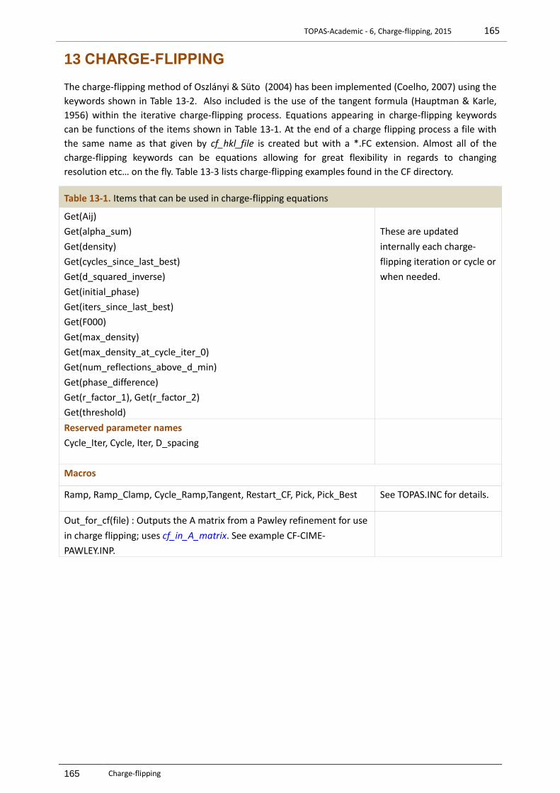
TOPAS-Academic - 6, Charge-flipping, 2015 165
165 Charge-flipping
13 CHARGE-FLIPPING
The charge-flipping method of Oszlányi & Süto (2004) has been implemented (Coelho, 2007) using the
keywords shown in Table 13-2. Also included is the use of the tangent formula (Hauptman & Karle,
1956) within the iterative charge-flipping process. Equations appearing in charge-flipping keywords
can be functions of the items shown in Table 13-1. At the end of a charge flipping process a file with
the same name as that given by cf_hkl_file is created but with a *.FC extension. Almost all of the
charge-flipping keywords can be equations allowing for great flexibility in regards to changing
resolution etc… on the fly. Table 13-3 lists charge-flipping examples found in the CF directory.
Table 13-1. Items that can be used in charge-flipping equations
Get(Aij)
Get(alpha_sum)
Get(density)
Get(cycles_since_last_best)
Get(d_squared_inverse)
Get(initial_phase)
Get(iters_since_last_best)
Get(F000)
Get(max_density)
Get(max_density_at_cycle_iter_0)
Get(num_reflections_above_d_min)
Get(phase_difference)
Get(r_factor_1), Get(r_factor_2)
Get(threshold)
These are updated
internally each charge-
flipping iteration or cycle or
when needed.
Reserved parameter names
Cycle_Iter, Cycle, Iter, D_spacing
Macros
Ramp, Ramp_Clamp, Cycle_Ramp,Tangent, Restart_CF, Pick, Pick_Best See TOPAS.INC for details.
Out_for_cf(file) : Outputs the A matrix from a Pawley refinement for use
in charge flipping; uses cf_in_A_matrix. See example CF-CIME-
PAWLEY.INP.
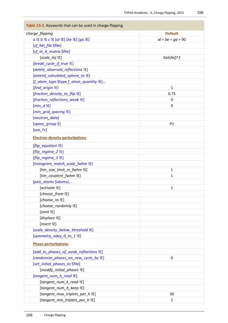
TOPAS-Academic - 6, Charge-flipping, 2015 166
166 Charge-flipping
Table 13-2. Keywords that can be used in charge-flipping.
charge_flipping Default
a !E b !E c !E [al !E] [be !E] [ga !E] al = be = ga = 90
[cf_hkl_file $file]
[cf_in_A_matrix $file]
[scale_Aij !E] Get(Aij)^2
[break_cycle_if_true !E]
[delete_observed_reflections !E]
[extend_calculated_sphere_to !E]
[f_atom_type $type f_atom_quantity !E]…
[find_origin !E] 1
[fraction_density_to_flip !E] 0.75
[fraction_reflections_weak !E] 0
[min_d !E] 0
[min_grid_spacing !E]
[neutron_data]
[space_group $] P1
[use_Fc]
Electron density perturbations
[flip_equation !E]
[flip_regime_2 !E]
[flip_regime_3 !E]
[histogram_match_scale_fwhm !E]
[hm_size_limit_in_fwhm !E] 1
[hm_covalent_fwhm !E] 1
[pick_atoms $atoms]...
[activate !E] 1
[choose_from !E]
[choose_to !E]
[choose_randomly !E]
[omit !E]
[displace !E]
[insert !E]
[scale_density_below_threshold !E]
[symmetry_obey_0_to_1 !E]
Phase perturbations
[add_to_phases_of_weak_reflections !E]
[randomize_phases_on_new_cycle_by !E] 0
[set_initial_phases_to $file]
[modify_initial_phases !E]
[tangent_num_h_read !E]
[tangent_num_k_read !E]
[tangent_num_h_keep !E]
[tangent_max_triplets_per_h !E] 30
[tangent_min_triplets_per_h !E] 1
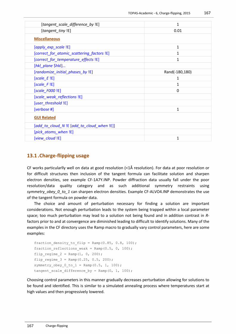
TOPAS-Academic - 6, Charge-flipping, 2015 167
167 Charge-flipping
[tangent_scale_difference_by !E] 1
[tangent_tiny !E] 0.01
Miscellaneous
[apply_exp_scale !E] 1
[correct_for_atomic_scattering_factors !E] 1
[correct_for_temperature_effects !E] 1
[hkl_plane $hkl]…
[randomize_initial_phases_by !E] Rand(-180,180)
[scale_E !E] 1
[scale_F !E] 1
[scale_F000 !E] 0
[scale_weak_reflections !E]
[user_threshold !E]
[verbose #] 1
GUI Related
[add_to_cloud_N !E [add_to_cloud_when !E]]
[pick_atoms_when !E]
[view_cloud !E] 1
13.1 . Charge-flipping usage
CF works particularlly well on data at good resolution (<1Å resolution). For data at poor resolution or
for difficult structures then inclusion of the tangent formula can facilitate solution and sharpen
electron densities, see example CF-1A7Y.INP. Powder diffraction data usually fall under the poor
resolution/data quality category and as such additional symmetry restraints using
symmetry_obey_0_to_1 can sharpen electron densities. Example CF-ALVO4.INP demonstrates the use
of the tangent formula on powder data.
The choice and amount of perturbation necessary for finding a solution are important
considerations. Not enough perturbation leads to the system being trapped within a local parameter
space; too much perturbation may lead to a solution not being found and in addition contrast in R-
factors prior to and at convergence are diminished leading to difficult to identify solutions. Many of the
examples in the CF directory uses the Ramp macro to gradually vary control parameters, here are some
examples:
fraction_density_to_flip = Ramp(0.85, 0.8, 100);
fraction_reflections_weak = Ramp(0.5, 0, 100);
flip_regime_2 = Ramp(1, 0, 200);
flip_regime_3 = Ramp(0.25, 0.5, 200);
symmetry_obey_0_to_1 = Ramp(0.5, 1, 100);
tangent_scale_difference_by = Ramp(0, 1, 100);
Choosing control parameters in this manner gradually decreases perturbation allowing for solutions to
be found and identified. This is similar to a simulated annealing process where temperatures start at
high values and then progressively lowered.

TOPAS-Academic - 6, Charge-flipping, 2015 168
168 Charge-flipping
13.1.1 ....Perturbations
Perturbations can be categorized as being of either phase, structure factor intensity or electron
density perturbations as shown in Table 13-2. There are two built in flipping regimes, flip_regime_2
and flip_regime_3, and one user defined regime flip_equation. Only one can be used and they all
modify the electron density. In the absence of a flipping regime the following is used:
for
for ,
(13-1)
where corresponds to the electron density threshold.
Using the tangent formula on either difficult structures or on data at poor resolution often leads to
uranium atom solutions. Uranium atom solutions can be avoided by modifying the electron density
using a flipping regime that dampens high electron densities or by using pick_atoms.
Using a large number of triplets per Eh value (a value for tangent_max_triplets_per_h greater than
100) reduces perturbation, increases occurrences of uranium atom solutions and increases the
chances of finding a solution after an initial phase randomization. A large number of triplets would
typically be used for poor resolution data; correspondingly a flipping regime that avoids uranium atom
solutions should be chosen.
Perturbations mostly increase randomness in the system with the exceptions of the tangent
formula, scale_density_below_threshold and histogram_match_scale_fwhm.
13.1.2 ....The Ewald sphere, weak reflections and CF termination
By default CF uses the minimum observed d spacing to define the Ewald sphere; alternatively min_d
can be used. The Ewald sphere can be increased using extend_calculated_sphere_to; this inserts
missing reflections and gives them the status of “weak” reflections. Weak reflections are also inserted
for missing reflections within the Ewald sphere. Weak reflection phases and structure factors can be
modified using scale_weak_reflections and add_to_phases_of_weak_reflections.
Reflections that have zero intensities according to the space group are not included in CF;
correspondingly the number of observed reflections removed are reported. Structure factor intensities
within a family of reflections are determined by averaging the observed structure factors intensities.
This averaging is also performed on calculated intensities each CF iteration for weak reflections.
Changing the space group is possible; changing the space group to a higher symmetry from that as
implied in the input hkl file often makes sense. Changing the space group to a lower symmetry implies
less symmetry and is useful for checking whether a significantly better R-factor is realized.
Typically a fraction of observed reflections are given the status of “weak” using
fraction_reflections_weak. When a solution is found and CF terminates a *.FC file is saved; this file
comprises structures factors that produced the best R-factor. A new CF process can be initiated with
phase information saved in the *.FC file using the Restart_CF macro. To further complete the structure
the new CF process may for example reduce perturbations in order to sharpen the electron density.
13.1.3 ....Powder data considerations
For powder data it is usually best to maximize the number of constraints due to poor data quality; it is
also best to use *.A files as generated by a Pawley refinement and to then use cf_in_A_matrix. No
weak observed reflections within the observed Ewald sphere should be assigned by setting
fraction_reflections_weak to zero. Instead weak reflections can be included by extending the Ewald
sphere with something like:
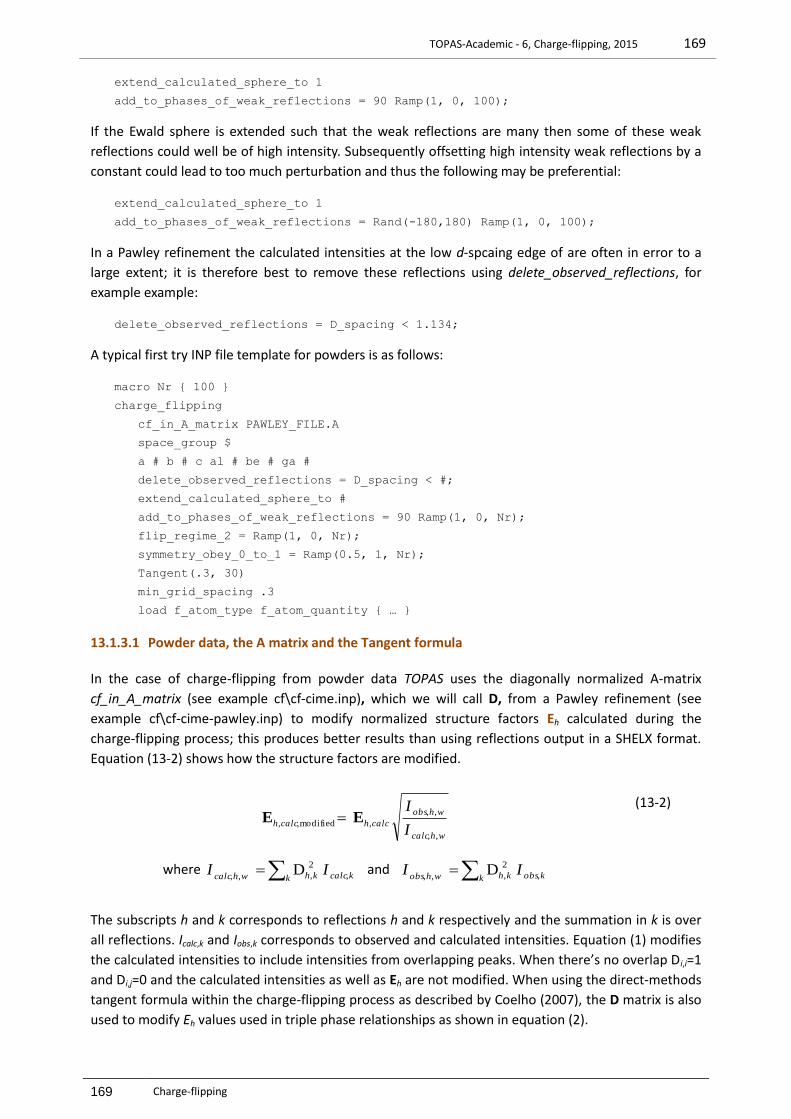
TOPAS-Academic - 6, Charge-flipping, 2015 169
169 Charge-flipping
extend_calculated_sphere_to 1
add_to_phases_of_weak_reflections = 90 Ramp(1, 0, 100);
If the Ewald sphere is extended such that the weak reflections are many then some of these weak
reflections could well be of high intensity. Subsequently offsetting high intensity weak reflections by a
constant could lead to too much perturbation and thus the following may be preferential:
extend_calculated_sphere_to 1
add_to_phases_of_weak_reflections = Rand(-180,180) Ramp(1, 0, 100);
In a Pawley refinement the calculated intensities at the low d-spcaing edge of are often in error to a
large extent; it is therefore best to remove these reflections using delete_observed_reflections, for
example example:
delete_observed_reflections = D_spacing < 1.134;
A typical first try INP file template for powders is as follows:
macro Nr { 100 }
charge_flipping
cf_in_A_matrix PAWLEY_FILE.A
space_group $
a # b # c al # be # ga #
delete_observed_reflections = D_spacing < #;
extend_calculated_sphere_to #
add_to_phases_of_weak_reflections = 90 Ramp(1, 0, Nr);
flip_regime_2 = Ramp(1, 0, Nr);
symmetry_obey_0_to_1 = Ramp(0.5, 1, Nr);
Tangent(.3, 30)
min_grid_spacing .3
load f_atom_type f_atom_quantity { … }
13.1.3.1 Powder data, the A matrix and the Tangent formula
In the case of charge-flipping from powder data TOPAS uses the diagonally normalized A-matrix
cf_in_A_matrix (see example cf\cf-cime.inp), which we will call D, from a Pawley refinement (see
example cf\cf-cime-pawley.inp) to modify normalized structure factors Eh calculated during the
charge-flipping process; this produces better results than using reflections output in a SHELX format.
Equation (13-2) shows how the structure factors are modified.
,,
,,
,modified,, whcalc
whobs
calchcalchI
IEE
where k kcalckhwhcalcII
,
2
,
,, D and k kobskhwhobs
II
,
2
,
,, D
(13-2)
The subscripts h and k corresponds to reflections h and k respectively and the summation in k is over
all reflections. Icalc,k and Iobs,k corresponds to observed and calculated intensities. Equation (1) modifies
the calculated intensities to include intensities from overlapping peaks. When there’s no overlap Di,i=1
and Di,j=0 and the calculated intensities as well as Eh are not modified. When using the direct-methods
tangent formula within the charge-flipping process as described by Coelho (2007), the D matrix is also
used to modify Eh values used in triple phase relationships as shown in equation (2).

TOPAS-Academic - 6, Charge-flipping, 2015 170
170 Charge-flipping
)(1 ,,modified,, hhcalchhobshobs qEqEE
where k khhq 2
,D
(13-3)
Eobs,h and Ecalc,h corresponds to tangent formula Eh values calculated from the observed and calculated
intensities respectively. Ecalc,h is typically not used in the tangent formula, however, intensities used for
determining Eobs,h can be grossly in error due to peak overlap. Equation (2) therefore influences triple
phase relationships by weighing Eobs,h by qh; when there’s no overlap qh=1 resulting in no modification.
When there’s significant overlap then qh is small and the influence of triple phase relationships using
the h reflection is reduced. Equation (2) also includes a (1- qh) portion of Ecalc,h thus stating that when
there’s significant overlap the calculated Eh is to be more trustworthy than the observed Eh. Equation
(13-3) corrects for errors in Eh when Iobs is similar to Icalc; this assists in reducing the goodness of fit
value thus enhancing the chances of solving the structure.
13.1.4 ....The algorithm of Oszlányi & Süto (2005) and F000
Normalized structure factors enhances the chances of finding a solution (Oszlányi & Süto, 2006) and
are realized by inclusion of f_atom_type’s and when correct_for_temperature_effects is non-zero.
Example CF-1A7Y-GABOR.INP implements the algorithm of Oszlányi & Süto (2005) with normalized
structure factors. In the original algorithm the amount of charge flipped is a function of the maximum
electron density; this can be realized using:
user_threshold = 0.2 Get(max_density_at_cycle_iter_0);
Get(max_density_at_cycle_iter_0) is a different value at the start of each CF process as phases are
chosen randomly. An alternative means of defining the threshold is:
fraction_density_to_flip 0.83
The CF process is sensitive to the threshold value. A value of 0.83 for fraction_density_to_flip is
optimum for 1a7y and produces a solution in ~1000 iterations. A solution is not found however at
0.75 or 0.85. To overcome this sensitivity the fraction_density_to_flip parameter could be ramped as a
function of iteration from a high value to a low value, or,
fraction_density_to_flip = Ramp(0.85, 0.8, 100);
Implementation of such a ramp solves 1a7y in ~2000 iterations.
F000 is allowed to float when scale_F000 is set to 1. In the Oszlányi & Süto (2005) algorithm a floating
F000 produces the best results for some structures but not for others (see section 13.2.3).
When the electron density is perturbed then a floating F000 often produces unfavourable
oscillations in R-factors. In general the electron density is best left unperturbed when scale_F000 is
non-zero. Example CF-1A7Y-GABOR.INP does not seem to solve at a lower resolution, try for example:
delete_observed_reflections = D_spacing < 1.1;
On the other hand when scale_F000 is zero then electron density perturbations are possible;
CF_1A7Y.INP solves 1a7y at 1.1 Angstrom (ie. include “delete_observed_reflections = D_spacing <
1.1”); CF_1A7Y.INP uses flip_regime_2 and the tangent formula.
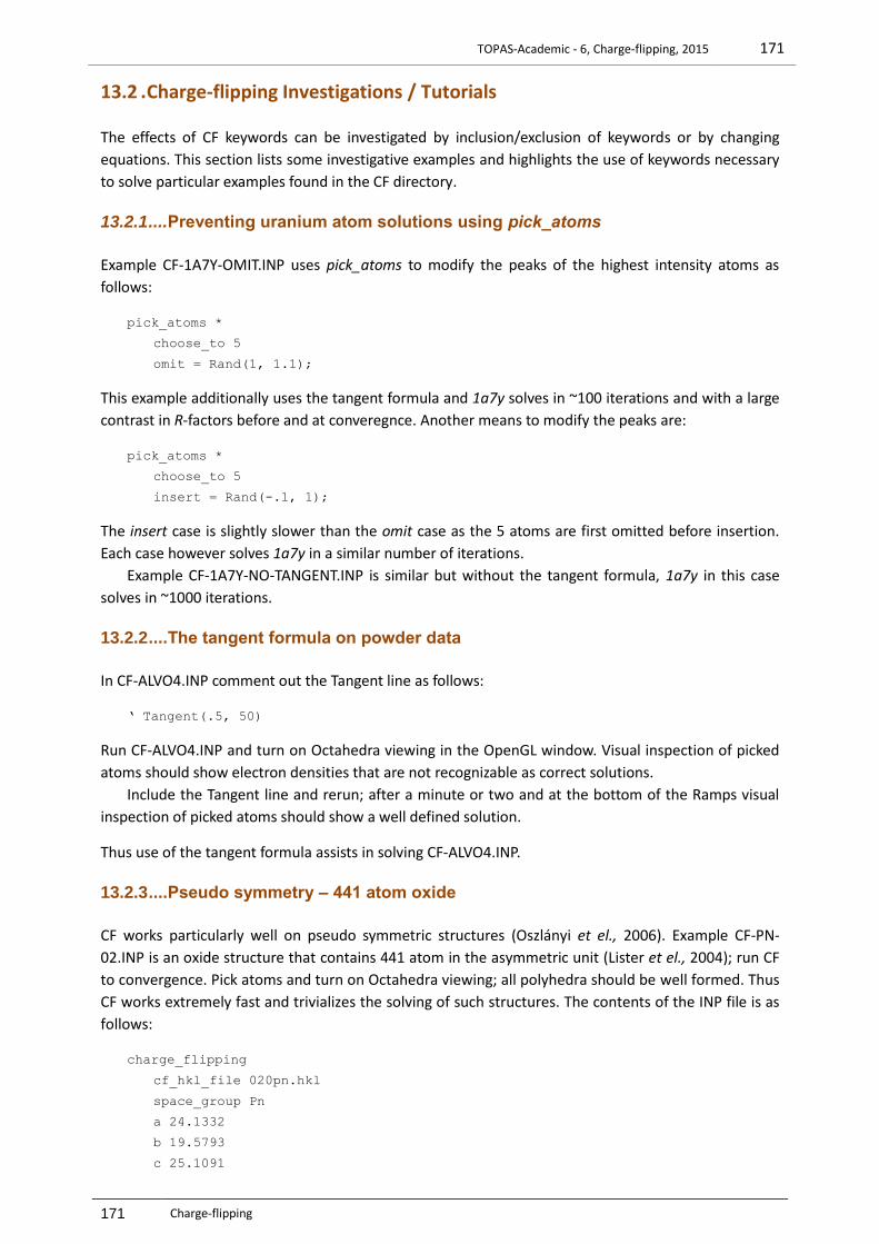
TOPAS-Academic - 6, Charge-flipping, 2015 171
171 Charge-flipping
13.2 . Charge-flipping Investigations / Tutorials
The effects of CF keywords can be investigated by inclusion/exclusion of keywords or by changing
equations. This section lists some investigative examples and highlights the use of keywords necessary
to solve particular examples found in the CF directory.
13.2.1 ....Preventing uranium atom solutions using pick_atoms
Example CF-1A7Y-OMIT.INP uses pick_atoms to modify the peaks of the highest intensity atoms as
follows:
pick_atoms *
choose_to 5
omit = Rand(1, 1.1);
This example additionally uses the tangent formula and 1a7y solves in ~100 iterations and with a large
contrast in R-factors before and at converegnce. Another means to modify the peaks are:
pick_atoms *
choose_to 5
insert = Rand(-.1, 1);
The insert case is slightly slower than the omit case as the 5 atoms are first omitted before insertion.
Each case however solves 1a7y in a similar number of iterations.
Example CF-1A7Y-NO-TANGENT.INP is similar but without the tangent formula, 1a7y in this case
solves in ~1000 iterations.
13.2.2 ....The tangent formula on powder data
In CF-ALVO4.INP comment out the Tangent line as follows:
‘ Tangent(.5, 50)
Run CF-ALVO4.INP and turn on Octahedra viewing in the OpenGL window. Visual inspection of picked
atoms should show electron densities that are not recognizable as correct solutions.
Include the Tangent line and rerun; after a minute or two and at the bottom of the Ramps visual
inspection of picked atoms should show a well defined solution.
Thus use of the tangent formula assists in solving CF-ALVO4.INP.
13.2.3 ....Pseudo symmetry – 441 atom oxide
CF works particularly well on pseudo symmetric structures (Oszlányi et el., 2006). Example CF-PN-
02.INP is an oxide structure that contains 441 atom in the asymmetric unit (Lister et el., 2004); run CF
to convergence. Pick atoms and turn on Octahedra viewing; all polyhedra should be well formed. Thus
CF works extremely fast and trivializes the solving of such structures. The contents of the INP file is as
follows:
charge_flipping
cf_hkl_file 020pn.hkl
space_group Pn
a 24.1332
b 19.5793
c 25.1091

TOPAS-Academic - 6, Charge-flipping, 2015 172
172 Charge-flipping
be 99.962
fraction_reflections_weak 0.4
symmetry_obey_0_to_1 .3
Tangent(.25, 30)
load f_atom_type f_atom_quantity
{
MO = 42 2;
P = (126 - 42) 2;
O = (441 - 126) 2;
}
The tangent formula is used to assist symmetry_obey_0_to_1 and to assist in finding the solution
faster; it is not necessary for this example however. The Oszlányi & Süto (2005) algorithm can be used
by replaceing symmetry_obey_0_to_1 and the Tangent line with the following:
scale_F000 1
fraction_reflections_weak .4
add_to_phases_of_weak_reflections 90
user_threshold = 0.15 Get(max_density_at_cycle_iter_0);
Slow convergence is then observed and the reason is the use of F000. This is opposite to the case of
1a7y in CF-1A7Y-GABOR.INP where F000 is necessary. Setting scale_F000 to zero greatly increases the
rate of convergence.
13.2.4 ....Origin finding and symmetry_obey_0_to_1
When symmetry_obey_0_to_1 is defined origin finding is performed each iteration of charge flipping.
Symmetry elements of the space group are used in finding an origin. On finding an origin the electron
density is shifted to a position that best matches the symmetry of the space group. Additionally a
restraint is placed on the electron density pixels forcing symmetry to be obeyed.
Run CF-AE14.INP to convergence; notice the P-1 symmetry. Remove symmetry_obey_0_to_1 and
run to convergence; the origin should now be arbitrary.
13.2.5 ....symmetry_obey_0_to_1 on poor resolution data
Run CF-AE5.INP until a solution is found; terminate CF, this saves the phase information to the file
AE5.FC.
Copy AE5.FC to AE5-SAVE.FC.
Place the following lines into the file CF-AE5-POOR.INP
set_initial_phases_to ae5-save.fc
randomize_initial_phases_by 0
This simply starts CF with optimum phase values. Also include the following line:
symmetry_obey_0_to_1 .75
Run CF-AE5-POOR.INP; the atom positions after picking should visually produce the correct result.
Comment out symmetry_obey_0_to_1 and rerun CF-AE5-POOR.INP. R-factors should diverge and
picked atoms should show a non-solution. Thus symmetry_obey_0_to_1 assists in solving CF-AE5-
POOR.INP.
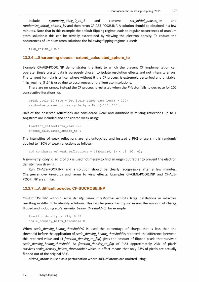
TOPAS-Academic - 6, Charge-flipping, 2015 173
173 Charge-flipping
Include symmetry_obey_0_to_1 and remove set_initial_phases_to and
randomize_initial_phases_by and then rerun CF-AE5-POOR.INP. A solution should be obtained in a few
minutes. Note that in this example the default flipping regime leads to regular occurrences of uranium
atom solutions; this can be trivially ascertained by viewing the electron density. To reduce the
occurrences of uranium atom solutions the following flipping regime is used:
flip_regime_3 0.5
13.2.6 ....Sharpening clouds - extend_calculated_sphere_to
Example CF-AE9-POOR.INP demonstrates the limit to which the present CF implementation can
operate. Single crystal data is purposely chosen to isolate resolution effects and not intensity errors.
The tangent formula is critical where without it the CF process is extremely perturbed and unstable.
“flip_regime_3 .5” is used due to occurrences of uranium atom solutions.
There are no ramps, instead the CF process is restarted when the R-factor fails to decrease for 100
consecutive iterations, or,
break_cycle_if_true = Get(iters_since_last_best) > 100;
randomize_phases_on_new_cycle_by = Rand(-180, 180);
Half of the observed reflections are considered weak and additionally missing reflections up to 1
Angstrom are included and considered weak using:
fraction_reflections_weak 0.5
extend_calculated_sphere_to 1
The intensities of weak reflections are left untouched and instead a Pi/2 phase shift is randomly
applied to ~30% of weak reflections as follows:
add_to_phases_of_weak_reflections = If(Rand(0, 1) < .3, 90, 0);
A symmetry_obey_0_to_1 of 0.7 is used not merely to find an origin but rather to prevent the electron
density from straying.
Run CF-AE9-POOR.INP and a solution should be clearly recognizable after a few minutes.
Change/remove keywords and rerun to view effects. Examples CF-CIME-POOR.INP and CF-AE5-
POOR.INP are similar.
13.2.7 ....A difficult powder, CF-SUCROSE.INP
CF-SUCROSE.INP without scale_density_below_threshold=0 exhibits large oscillations in R-factors
resulting in difficult to identify solutions; this can be prevented by increasing the amount of charge
flipped and including scale_density_below_threshold=0, for example
fraction_density_to_flip 0.83
scale_density_below_threshold 0
When scale_density_below_threshold=0 is used the percentage of charge that is less than the
threshold before the application of scale_density_below_threshold is reported; the difference between
this reported value and (1-fraction_density_to_flip) gives the amount of flipped pixels that survived
scale_density_below_threshold. At fraction_density_to_flip of 0.83 approximately 23% of pixels
survives scale_density_below_threshold=0 which in effect means that only 23% of pixels are actually
flipped out of the original 83%.
picked_atoms is used as a perturbation where 30% of atoms are omitted using:
TOPAS-Academic - 6, Charge-flipping, 2015 174
174 Charge-flipping
pick_atoms *
activate = Cycle_Iter == 0;
insert = If(Rand(0, 1) > 0.3, 10, 0);
Note that atoms are inserted at an intensity that is 10 times the average intensity. This increases the
weight of inserted atoms relative to electron density noise. It also initially gives more weight to weak
reflections.
Use of scale_density_below_threshold often results in CF requiring more interations to solution; a
solution however is preferable to no solution.
13.2.8 ....Increasing contrast in R-factors
The act of flipping introduces an appreciable amount of unwanted high frequencies in the structure
factors. This effect can be reduced by dampening high frequencies using apply_exp_scale which is ON
by default. apply_exp_scale changes R-factors and not phases, directions taken by CF are unchanged.
Run CF-1A7Y.INP until convergence. The difference in R-factors before and at convergence should
be ~0.39 (ie. 0.81 and 0.42). Turn OFF apply_exp_scale by including the following line:
apply_exp_scale 0
Rerun CF-1A7Y.INP until convergence. The difference in R-factors before and at convergence should
now be ~0.29 (ie. 0.81 and 0.52). Thus apply_exp_scale increases contrast in R-factors. Note that most
of the increase seems to be realized from d-spacings less than 1 Angstrom.
13.3 . Charge Flipping and neutron_data
The neutron_data keyword informs the charge flipping routine that neutron scattering lengths are to be used. It
also results in the following default neutron flipping routine being used:
flip_equation =
If(And(Get(density) < Get(threshold), Get(density) > 0.4
Get(min_density)),
-Get(density),
Get(density)
);
The flip_neutron equation defines the 0.4 in the above equation. For example, the following can be used to
change the default to 0.5:
flip_neutron = 0.5;
The tangent formula is made less accurate due to the negative scattering of H atoms. However, if positive
scattering lengths are dominant then the tangent formula can stabilize refinement. For example, try:
Tangent(.3, 30)
tangent_scale_difference_by = Ramp(1, 0, Nc);
See test_examples\cf\neutron-cime\cf-neutron.inp
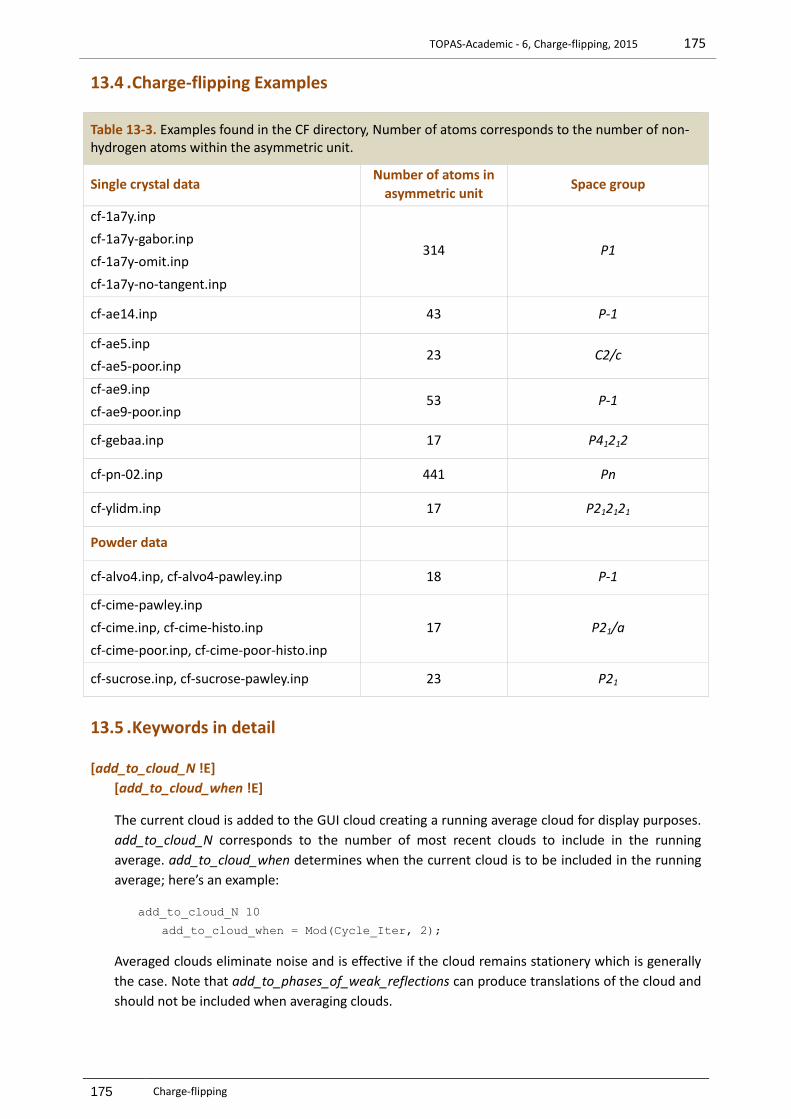
TOPAS-Academic - 6, Charge-flipping, 2015 175
175 Charge-flipping
13.4 . Charge-flipping Examples
Table 13-3. Examples found in the CF directory, Number of atoms corresponds to the number of non-hydrogen atoms within the asymmetric unit.
Single crystal data Number of atoms in
asymmetric unit Space group
cf-1a7y.inp
cf-1a7y-gabor.inp
cf-1a7y-omit.inp
cf-1a7y-no-tangent.inp
314 P1
cf-ae14.inp 43 P-1
cf-ae5.inp
cf-ae5-poor.inp 23 C2/c
cf-ae9.inp
cf-ae9-poor.inp 53 P-1
cf-gebaa.inp 17 P41212
cf-pn-02.inp 441 Pn
cf-ylidm.inp 17 P212121
Powder data
cf-alvo4.inp, cf-alvo4-pawley.inp 18 P-1
cf-cime-pawley.inp
cf-cime.inp, cf-cime-histo.inp
cf-cime-poor.inp, cf-cime-poor-histo.inp
17 P21/a
cf-sucrose.inp, cf-sucrose-pawley.inp 23 P21
13.5 . Keywords in detail
[add_to_cloud_N !E]
[add_to_cloud_when !E]
The current cloud is added to the GUI cloud creating a running average cloud for display purposes.
add_to_cloud_N corresponds to the number of most recent clouds to include in the running
average. add_to_cloud_when determines when the current cloud is to be included in the running
average; here’s an example:
add_to_cloud_N 10
add_to_cloud_when = Mod(Cycle_Iter, 2);
Averaged clouds eliminate noise and is effective if the cloud remains stationery which is generally
the case. Note that add_to_phases_of_weak_reflections can produce translations of the cloud and
should not be included when averaging clouds.

TOPAS-Academic - 6, Charge-flipping, 2015 176
176 Charge-flipping
[add_to_phases_of_weak_reflections !E]
Allows for modification to phases of weak reflections. For example, to add /2 to the phases of
weak reflections then the following could be used:
add_to_phases_of_weak_reflections 90
When add_to_phases_of_weak_reflections is defined then the intensities of weak reflections are
not set to zero; instead they are left untouched meaning that their intensities are set to the values
as determined by the inverse Fourier transform. See also scale_weak_reflections.
[apply_exp_scale !E]
Determines a and b each CF iteration such that the following is a minimum:
R-factor = ∑| a Exp(b / D_spacing^2) Fc – Fo |
where Fc and Fo are the calculated and observed moduli respectively. Use of apply_exp_scale
corrects R-factors in case of an incorrect temperature factor correction as applied when
normalizing structure factors. Use of apply_exp_scale typically increases the difference between R-
factors prior to and at convergence. apply_exp_scale is used by default, setting it to zero prevents
its use.
[cf_hkl_file $file]
Defines the input hkl file.
[cf_in_A_matrix $file [scale_Aij !E] ]
Data input is from a file created using out_A_matrix from a previous Pawley refinement. The
correlations in $file are used to partition intensities during each iteration of charge-flipping. This
partitioning is applied to structure factors as used by CF and as used by the tangent formula.
scale_Aij can be used to modify the A matrix off-diagonal coefficients, here are some examples:
scale_Aij = Get(Aij);
scale_Aij = Get(Aij)^2; ‘ the default
scale_Aij = 0; ‘ Equivalent to using a Pawley generated hkl file
CF on powder data can also be initiated using standard hkl files.
[break_cycle_if_true !E]
Interrupts charge flipping to execute randomize_phases_on_new_cycle_by. Cycle_Iter is set to zero
and Cycle is incremented.
[correct_for_atomic_scattering_factors !E]
Structure factors are normalized when non-zero and when f_atom_type’s are defined. By default
structure factors are normalized.
[correct_for_temperature_effects !E]
Attempts to remove isotropic temperature effects from the structure factors.
correct_for_temperature_effects is ON by default, setting it to zero will prevent the correction.
Normalized structure factors are realized when correct_for_temperature_effects is ON and the unit
cell contents is defined using f_atom_type and f_atom_quantity.
TOPAS-Academic - 6, Charge-flipping, 2015 177
177 Charge-flipping
[delete_observed_reflections !E]
Reflections are deleted before entering CF according to delete_observed_reflections; it can be a
function of D_spacing, for example:
delete_observed_reflections = D_spacing < 1.1;
Once deleted, observed reflections cannot be reinstated by changing min_d.
[extend_calculated_sphere_to !E]
Used to sharpen electron density clouds by filling in missing reflections; added reflections are
given the status of “weak”. extend_calculated_sphere_to can be used in conjunction with
scale_weak_reflections and add_to_phases_of_weak_reflections to modify “weak” reflection
magnitudes and phases respectively (see section 13.2.6); here’s an example:
extend_calculated_sphere_to 1
add_to_phases_of_weak_reflections = If(Rand(0, 1) < .3, 90, 0);
[f_atom_type $type f_atom_quantity !E]…
Defines atom types and number of atoms within the unit cell; used by the tangent formula in
determining Eh values and by the OpenGL display for picking atoms. For the tangent formula then
realtive quantities are important.
[find_origin !E]
If defined and non-zero then origin finding is turned ON. symmetry_obey_0_to_1 defines
find_origin by default. symmetry_obey_0_to_1 can be used without find_origin by defining and
setting find_origin to zero.
[flip_equation !E]
Allwows for a user defined flip; here’s an example:
flip_equation =
If(Get(density) < Get(threshold), -Get(density), Get(density));
[flip_regime_2 !E]
The elctron density is modified according to Eq. (13-1) and then further modified using:
egime_2)Get(flip_r 2
max
3
flip_regime_2 is typically ramped from 1 to 0.
[flip_regime_3 !E]
The elctron density is modified according to Eq. (13-1) and then further modified using:
for egime_3))Get(flip_r ,Min(
for ,
max
A value of 0.5 for flip_regime_3 introduces little perturbation whilst reducing the occurance of
uranium atom solutions. It is recommended that flip_regime_3 be used in cases where
flip_regime_2 produces uranium atom solutions. An additional perturbation, such as
“add_to_phases_of_weak_reflections=90;” may be necessary.

TOPAS-Academic - 6, Charge-flipping, 2015 178
178 Charge-flipping
[fraction_density_to_flip !E]
The amount of charge flipped is fractionally based. A value of 0.6, for example, sets the threshold
such that the sign of the lowest 60% of charge is changed. Get(threshold) can be used to retrieve .
[fraction_reflections_weak !E]
Defines the fraction of observed reflections to flag as “weak”. When scale_weak_reflections,
add_to_phases_of_weak_reflections and extend_calculated_sphere_to are all not defined then
intensities of weak reflections are set to zero effectively removing them from the charge flipping
process. Otherwise intensities of weak reflections are not set to zero; instead they are left
untouched prior to scale_weak_reflections and add_to_phases_of_weak_reflections and space
group family averaging.
[histogram_match_scale_fwhm !E] [hm_size_limit_in_fwhm !E]
[hm_covalent_fwhm !E]
An implementation of Histogram Matching (Baerlocher et al., 2007) where the distribution of
pixels within the unit cell is restrained to one that matches Gaussian atoms with intensities
corresponding to the atoms defined by f_atom_type‘s. The Histogram matching operation is
performed when histogram_match_scale_fwhm evaluates to a non-zero value. Subsequently the
full width at half maximum (FWHM) of the Gaussians (obtained from the file ATOM_RADIUS.DEF)
is scaled by histogram_match_scale_fwhm. hm_size_limit_in_fwhm corresponds to the extent to
which the Gaussians are calculated in units of FWHM. Covalent radii is used if hm_covalent_fwhm
evaluates to a non-zero value otherwise ionic radii is used. An example use is as follows:
histogram_match_scale_fwhm = If(Mod(Cycle_Iter, 3), 0, 1);
hm_size_limit_in_fwhm 1
hm_covalent_fwhm 1
Reported on is the fraction of pixels modified; values of 1 for both histogram_match_scale_fwhm
and hm_size_limit_in_fwhm seem optimal where typically ~15 to 20% of pixels are modified. Use
of histogram matching should produce R-factors at convergence that are equal to or than less R-
factors produced when not using histogram matching. Histogram matching sharpens the electron
density cloud for data at poor resolution (see examples CF-CIME-HISTO.INP and CF-CIME-POOR-
HISTO.INP).
[min_d !E]
Determines in Angstroms the resolution of observed reflections to work with; only observed
reflections with a d-spacing above min_d are considered. min_d is evaluated each CF iteration.
Get(num_observed_reflections_above_d_min) is updated when a change in min_d is detected. See
also extend_calculated_sphere_to and delete_observed_reflections.
[min_grid_spacing !E]
If defined then the grid spacing used is set to the smaller of min_d/2 and min_grid_spacing; useful
for obtaining many grid points for graphical purposes.
[neutron_data]
Signals that the input data is of neutron type. Used in the picking of atoms and additionally Eh
values are not corrected from any defined f_atom_type and f_atom_quantity keywords.

TOPAS-Academic - 6, Charge-flipping, 2015 179
179 Charge-flipping
[pick_atoms $atoms]...
[activate !E]
[choose_from !E]
[choose_to !E]
[choose_randomly !E]
[omit !E]
[displace !E]
[insert !E]
pick_atoms modifies the electron density based on picked atoms. $atom corresponds to the atom
types to be operated on; it can contain the wild card character ‘*’ and the negation character ‘!’,
see section 10.18 for details. The operations of pick_atoms are invoked when activate evaluates to
a non-zero value; for example,
pick_atoms “O C”
activate = Mod(Cycle_Iter, 20) == 0;
The picking routine will attempts to locate the atom types found in $atom based on the intensities
of picked atoms and the scattering power of the atoms defined in f_atom_type. For example,
load f_atom_type f_atom_quantity { Ca 2 O 10 C 12 }
pick_atoms “O C”
Here 2 Ca atoms are first picked and then 10 O atoms and then 12 C atoms. The picked atoms
operated on will be the O and C atoms with the Ca atoms ignored.
choose_from and choose_to can be used to limit the number of atoms operated on. Note, that
picked atoms within a particular pick_atoms are sorted in decreasing intensity order. For example,
to not operate on the first thee O atoms and the last 2 C atoms then the following could be used:
choose_from 4
choose_to 20
choose_randomly further reduces the atoms operated on and is executed after choose_from and
choose_to.
omit removes operated on atoms from the electron density. Atoms can be partially removed by
setting omit to values less than 1. Values greater than 1 can also be used, the effect is to change
the sign of the electron density. omit operating on a few of the highest intensity atoms is an
extremely effective means of preventing the occurance of uranium atom solutions, see CF-1A7Y-
OMIT.INP; for example:
pick_atoms *
choose_to 5
omit = Rand(1, 1.1);
Omitting atoms randomly is a technique referred to as “random omit maps“ in ShelXD, (Schneider
and Sheldrick, 2002).
insert inserts operated on atoms; a value of 1 inserts the atoms with an intensity that is equal
to the average of the picked atoms. Values of less than 1 descreases the intensity of the inserted
atoms. When insert is defined then omit is internally defined if it does not already exist. Thus,
atoms are removed before insertion by default.
displace (in Angstroms) displaces atom positions from their picked positions; it is evaluated
before insert. For example, to randomly displace atoms by 0.3 Angstroms then the following could
be used:
TOPAS-Academic - 6, Charge-flipping, 2015 180
180 Charge-flipping
displace = Rand(0.4, 0.6);
insert 1
There can be more than one occurance of pick_atoms, for example to limit uranium atom solutions
then the following can be used:
pick_atoms *
choose_to 5
insert = Rand(-.1, 1);
To further randomly remove ~33% of atoms then the following could additionally be used:
break_cycle_if_true = Get(iters_since_last_best) > 10;
pick_atoms *
activate = Cycle_Iter == 0;
insert = If(Rand(0, 1) > 0.33, 10, 0);
Note that in this example atoms are inserted at ten times the average picked intensity; this simply
gives more weight to picked atoms relative to electron density noise. Additionaly weak reflections
are also given more weighting.
[pick_atoms_when !E]
Atoms are picked in the OpenGL display when pick_atoms_when evaluates to a non-zero value;
here’s an example:
pick_atoms_when = Mod(Cycle_Iter + 1, 10) == 0;
Note that picking can be manually initiated from the Cloud dialog of the OpenGL display. A text
description of picked atoms can be obtained by opening the “Temporary output” text window of
the OpenGL window.
[randomize_initial_phases_by !E]
Initializes phases. To start a process with already saved phase information then the following
could be used:
set_initial_phases_to aleady_saved.fc
randomize_initial_phases_by 0 ' this has a default of Rand(-180,180)
[randomize_phases_on_new_cycle_by !E]
randomize_phases_on_new_cycle_by = Rand(-180, 180); ‘ an example
[scale_density_below_threshold !E]
Electron density pixels that are less than the threshold value are scaled by
scale_density_below_threshold. Values for scale_density_below_threshold thata re less than 1
tends to sharpen the electron density and to reduce large oscillations in R-factors; the latter occurs
for bad data, see example CF-SUCROSE.INP. A value of zero for scale_density_below_threshold
results in “low density elimination“ simlar to that of Shiono & Woolfson (1992).
[scale_E !E]
Normalized structure factors (Eh values) are a function of correct_for_temperature_effects and unit
cell contents. scale_E allows for an additional scaling of Eh values.

TOPAS-Academic - 6, Charge-flipping, 2015 181
181 Charge-flipping
[scale_F !E]
CF works with normalized structure factors by default. scale_F is an additional scaling of structure
factors. The defualt scale_F broadens electron density peaks to avoid pixilation effects and is given
by:
scale_F = Exp(-0.2 Get(d_squared_inverse));
[scale_F000 !E]
Scale should be set to 1 for compliance with the algorithm of Oszlányi & Süto (2004). When
scale_F000 is non_zero then modifcations to the electron density produces unfavourable effects.
[scale_weak_reflections !E]
By default weak reflection structure factors are set to zero; however when either
scale_weak_reflections or add_to_phases_of_weak_reflections is defined then weak reflections
structure factors are instead modified accordingly, for example:
scale_weak_reflections = Rand(-0.2, 0.4);
scale_weak_reflections or add_to_phases_of_weak_reflections can be a function of D_spacing.
[set_initial_phases_to $file]
[modify_initial_phases !E]
Sets initial phases to those appearing in $file. Typically $file corresponds to a *.FC file saved in a
previous charge-flipping process. modify_initial_phases is executed each iteration of CF; it can be
used to restrain the phases of $file. For example,
modify_initial_phases =
Get(initial_phase) + Min(Abs(Get(phase_difference)), 45);
where phase_difference corresponds to the difference between the current phase and the initial
phase; it has a value between ±90º. modify_initial_phases can be used to constrain phases to
those as determined by HRTEM (Baerlocher et al., 2007).
[space_group $]
If defined then the cf_hkl_file is assumed to comprise merged hkls corresponding to the defined
space group; otherwise the cf_hkl_file is assumed to be of space group type P1.
[symmetry_obey_0_to_1 !E]
If a space group is defined then symmetry is adhered to according to symmetry_obey_0_to_1.
symmetry_obey_0_to_1 can be throught of as a real space electron density restraint; its value
should range between 0 and 1. If 1 then symmetry is obeyed 100%; if 0 then for a particular set of
equivalent grid points, as determined by the equivalent positions of the space group, an average
density avg is obtained. The electron densities on the grid points are then adjusted as follows:
new = (1 - symmetry_obey_0_to_1) + symmetry_obey_0_to_1 avg
The text output 'symmetry error' as displayed when symmetry_obey_0_to_1 is used is defined as
follows:
'symmetry error' = avg
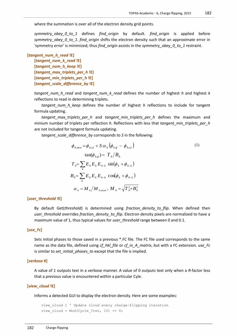
TOPAS-Academic - 6, Charge-flipping, 2015 182
182 Charge-flipping
where the summation is over all of the electron density grid points.
symmetry_obey_0_to_1 defines find_origin by default. find_origin is applied before
symmetry_obey_0_to_1. find_origin shifts the electron density such that an approximate error in
'symmetry error' is minimized; thus find_origin assists in the symmetry_obey_0_to_1 restraint.
[tangent_num_h_read !E] [tangent_num_k_read !E]
[tangent_num_h_keep !E]
[tangent_max_triplets_per_h !E]
[tangent_min_triplets_per_h !E]
[tangent_scale_difference_by !E]
tangent_num_h_read and tangent_num_k_read defines the number of highest h and highest k
reflections to read in determining triplets.
tangent_num_h_keep defines the number of highest h reflections to include for tangent
formula updating.
tangent_max_triplets_per_h and tangent_min_triplets_per_h defines the maximum and
minium number of triplets per reflection h. Reflections with less that tangent_min_triplets_per_h
are not included for tangent formula updating.
tangent_scale_difference_by corresponds to S in the following:
cfhtfhhcfhnewh S ,,,,
)tan( , tfh hh BT
k
khkkhkhh EEET sin
k
khkkhkhh EEEB cos
max, hhh MM , 22 hhh BTM
(1)
[user_threshold !E]
By default Get(threshold) is determined using fraction_density_to_flip. When defined then
user_threshold overrides fraction_density_to_flip. Electron density pixels are normalized to have a
maximum value of 1, thus typical values for user_threshold range between 0 and 0.1.
[use_Fc]
Sets initial phases to those saved in a previous *.FC file. The FC file used corresponds to the same
name as the data file, defined using cf_hkl_file or cf_in_A_matrix, but with a FC extension. use_Fc
is similar to set_initial_phases_to except that the file is implied.
[verbose #]
A value of 1 outputs text in a verbose manner. A value of 0 outputs text only when a R-factor less
that a previous value is encountered within a particular Cyle.
[view_cloud !E]
Informs a detected GUI to display the electron density. Here are some examples:
view_cloud 1 ' Update cloud every charge-flipping iteration
view_cloud = Mod(Cycle_Iter, 10) == 0;

TOPAS-Academic - 6, Indexing, 2015 183
183 Indexing
14 INDEXING
The following algorithm is based on the iterative method of Coelho (2003). Unlike lp_serach it requires
the extraction of d-spacings. The INDEXING directory contains example INP files, for example:
index_zero_error
try_space_groups "2 75"
load index_d {
8.912
7.126
4.296
…
}
Individual space groups can be tried or for simplicity all of the Bravais lattices can be tried by placing
them in the INP file using the standard macros as follows:
Bravais_Cubic_sgs
Bravais_Trigonal_Hexagonal_sgs
Bravais_Tetragonal_sgs
Bravais_Orthorhombic_sgs
Bravais_Monoclinic_sgs
Bravais_Triclinic_sgs
To try all unique extinction subgroup spacegroups, a more exhaustive approach, then the following
macros can be used:
Unique_Cubic_sgs
Unique_Trigonal_Hexagonal_sgs
Unique_Tetragonal_sgs
Unique_Orthorhombic_sgs
Unique_Monoclinic_sgs
Unique_Triclinic_sgs
On termination of Indexing a *.NDX file is created with a name corresponding to the name of the INP
file and placed in the same directory as the INP file. The *.NDX file contains solutions found as well as a
detailed summary of the best 20 solutions. Here’s an example of an NDX file:
' Indexing method - Alan Coelho (2003), J. Appl. Cryst. 36, 86-95
' Time: 2.015 seconds
'Sg Status UNI Vol Gof Zero Lps...
Indexing_Solutions_With_Zero_Error_2 {
0) P42/nmc 3 0 1187.321 38.82 0.0000 11.1924 ...
1) P42/nmc 3 0 1187.057 38.64 0.0000 11.1896 ...
2) P42/nmc 3 0 1187.458 38.61 0.0000 11.1914 ...
...
}
/*
======================================================================
0) P-1 0 985.652 30.80 0.0111 7.0877 ...
h k l dc do do-dc 2Thc 2Tho 2Tho-2Thc
0 0 1 15.857 15.830 -0.027 5.569 5.578 0.009
0 1 0 8.765 8.750 -0.015 10.084 10.101 0.017
0 0 2 7.928 7.910 -0.018 11.151 11.177 0.026
0 1 1 7.788 7.780 -0.008 11.352 11.364 0.012
0 -1 1 7.559 7.560 0.001 11.698 11.696 -0.002
...
*/

TOPAS-Academic - 6, Indexing, 2015 184
184 Indexing
14.1 . Figure of merit
The figure of merit M used in indexing is as follows:
1 1 2
,
2
,
2
min,uni i iiciooco QddNNdNM
where j jioi wwNQ
(14-1)
Where do and dc are the observed and calculated d-spacings, No and Nc the number of observed and
calculated lines used, Nuni the number of unindexed lines found and the summations are over the used
observed indexing lines. Qi is a weighting that assists in the determination of extinction subgroups
where wi could for example be the inverse of the error in the peak positions from a Pawley refinement
(see indexing\MgIr\index.inp). The keyword index_I corresponds to wi. The formulation of Qi is such
that with or without Qi the figure of merit M is of the same order of magnitude. The reciprocal-space
lattice relationship solved during the indexing process (Coelho, 2000) includes Q as follows:
22
222
/ ))sin(2 )λ / (4 )360π(
(
ohklhkle
klhlhkllkkhh
dWWθZ
k lX h lXk hX lXkXhX
where 2 hkl
m
ohklhkl dQW
(14-2)
14.2 . Extinction subgroup determination
At the end of an indexing further indexing runs are internally performed across extinction subgroups
(see section 14.8) in an attempt to determine the most likely subgroup. These internal runs are seeded
with already determined lattice parameters and in most cases the correct extinction subgroup is
obtained without the need for Qi in equation (14-1). Extinction subgroups can be explicitly searched
using the macro defined TOPAS.INC, see Unique_Orthorhombic_sgs for example.
14.3 . Reprocessing solutions - DET files
Details of solutions can be obtained at a later stage by including solution lines found in the NDX file
into the INP file. For example, supposing details of solutions 50 and 51 were sought then the following
(see example INDEXING\EX10.INP) could be used:
index_lam 1.540596
index_zero_error
try_space_groups 2
Indexing_Solutions_With_Zero_Error_2 {
50) P-1 1 0 2064.788 9.74 0.0000 ...
51) P-1 3 0 3128.349 9.61 0.0115 ...
}
load index_d {
15.83 good
8.75
7.91
...
}
After running this INP file a *.DET file is created containing details of the supplied solutions.

TOPAS-Academic - 6, Indexing, 2015 185
185 Indexing
14.4 . Keywords and data structures
The data structures for indexing are as follows:
Tindexing
[index_lam !E1.540596]
[index_min_lp !E2] [index_max_lp !E]
[index_max_Nc_on_No !E5]
[index_max_number_of_solutions #3000]
[index_max_th2_error !E0.05]
[index_max_zero_error #0.2]
[index_th2 !E | index_d !E]…
[index_I E1 [good]]
[index_x0 !E]
[index_zero_error]
[no_extinction_subgroup_search]
[seed]
[try_space_groups $]...
[x_angle_scaler #0.1]
[x_scaler #]
Values for most keywords are automatically determined or have defaults (appearing as numbers
above) adequate for difficult indexing problems. In the following example from UPPW (service
provided by Armel Le Bail to the SDPD mailing list at http://sdpd.univ-lemans.fr/uppw/) only a few
keywords are necessary. Also note the use of the dummy keyword; this allows for the exclusion of 2
and I values without having to edit the columns of data.
seed
index_lam 0.79776
index_zero_error
index_max_Nc_on_No 6
try_space_groups 3
load index_th2 dummy dummy index_I dummy {
' d (A) 2Theta Height Area FWHM
1.724 26.50645 2758.3 23303.7 0.0450
2.646 17.27733 150393.8 747063.6 0.0250
3.235 14.13204 98668.8 493153.7 0.0250
3.417 13.37776 11102.6 53185.0 0.0250
5.190 8.80955 782.7 3910.9 0.0250
...
}
14.5 . Keywords in detail
[index_lam !E1.540596]
Defines the wavelength in Å.
[index_min_lp !E2.5] [index_max_lp !E]
Defines the minimum and maximum allowed lattice parameters. Typically the maximum is
determined automatically.
TOPAS-Academic - 6, Indexing, 2015 186
186 Indexing
[index_max_Nc_on_No !E5]
Determines the maximum ratio of the number of calculated to observed lines. The value of 6
allows for up to 83% of missing lines.
[index_max_number_of_solutions #1000]
The number of best solutions to keep.
[index_max_th2_error !E0.05]
Used for determining impurity lines (un-indexed lines UNI in *.NDX). Large values, 1 for example,
forces the consideration of more observed input lines. For example if it is know that there are
none or maybe just one impurity line then a large value for index_max_th2_error will speed up the
indexing procedure.
[index_max_zero_error !E0.2]
Excludes solutions with zero errors greater than index_max_zero_error.
[index_th2 !E | index_d !E]…
[index_I E1 [good]]
index_th2 or index_d defines a reflection entry in 2 degrees or d-spacing in Å.
index_I is typically set to the area under the peak; it is used to weight the reflection.
good signals that the corresponding d-spacing is not an impurity line. A single use of good on a
large d-spacing decreases the number of possible solutions and hence speeds up the indexing
process (see examples INDEXING\EX10.INP).
[index_x0 !E]
Defines Xhh in the reciprocal lattice equation of (14-1). In a triclinic lattice the largest d-spacing can
probably be indexed as 100 or 200 etc. Thus
index_x0 = 1/(dmax)^2;
speeds up the indexing process (if, in this case, the first line can be indexed as 100) and
additionally the chances of finding the correct solution is enhanced. Example EX13.INP
demonstrates this. Note that if the data is in 2Th degrees then the following can be used:
index_x0 = (2 Sin(2Thmin Pi/360) / wavelength))^2;
The two macros Index_x0_from_d and Index_x0_from_th2 simplify the use of index_x0.
[index_zero_error]
Includes a zero error.
[no_extinction_subgroup_search]
By default Extinction subgroup determination is performed at the end of an indexing run; this can
be negated by defining no_extinction_subgroup_search keyword.
[seed]
Seeds the random number generator.
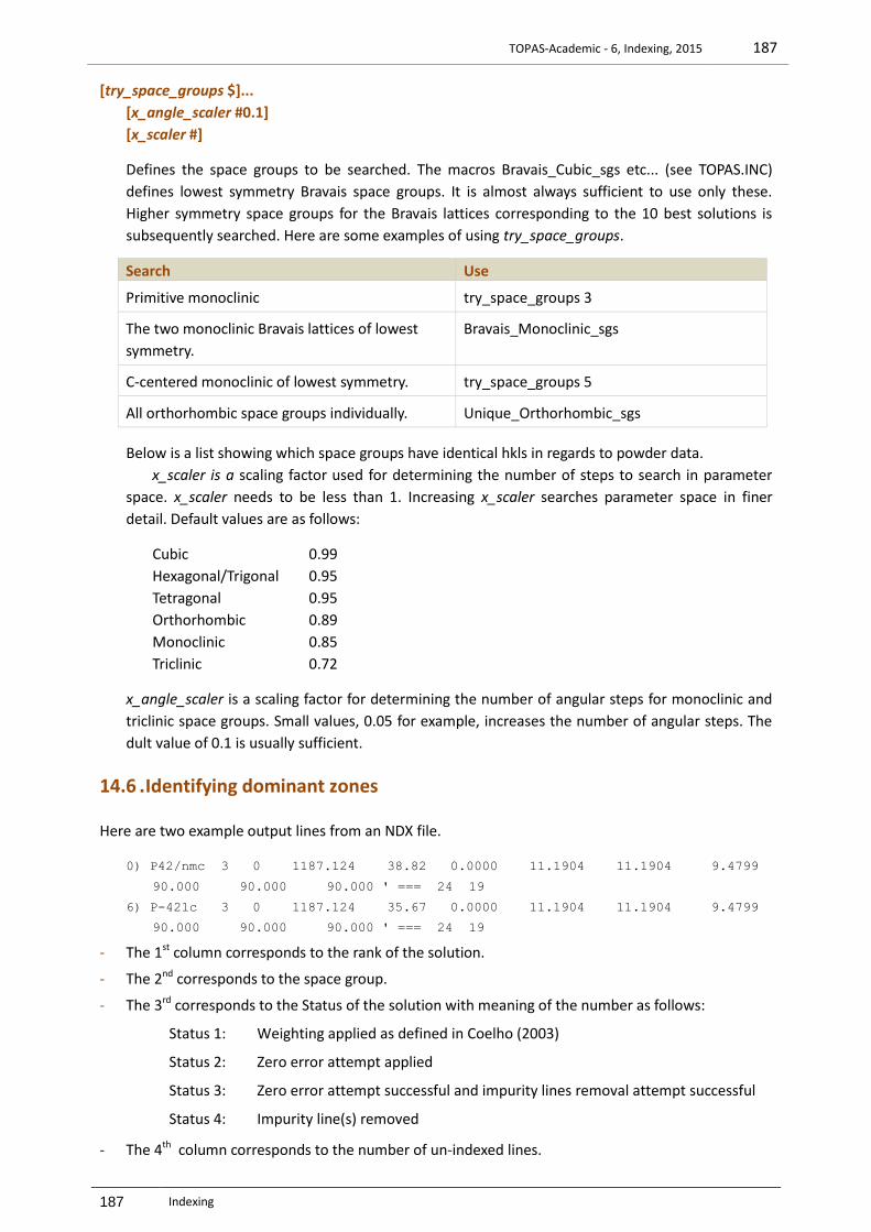
TOPAS-Academic - 6, Indexing, 2015 187
187 Indexing
[try_space_groups $]...
[x_angle_scaler #0.1]
[x_scaler #]
Defines the space groups to be searched. The macros Bravais_Cubic_sgs etc... (see TOPAS.INC)
defines lowest symmetry Bravais space groups. It is almost always sufficient to use only these.
Higher symmetry space groups for the Bravais lattices corresponding to the 10 best solutions is
subsequently searched. Here are some examples of using try_space_groups.
Search Use
Primitive monoclinic try_space_groups 3
The two monoclinic Bravais lattices of lowest
symmetry.
Bravais_Monoclinic_sgs
C-centered monoclinic of lowest symmetry. try_space_groups 5
All orthorhombic space groups individually. Unique_Orthorhombic_sgs
Below is a list showing which space groups have identical hkls in regards to powder data.
x_scaler is a scaling factor used for determining the number of steps to search in parameter
space. x_scaler needs to be less than 1. Increasing x_scaler searches parameter space in finer
detail. Default values are as follows:
Cubic 0.99
Hexagonal/Trigonal 0.95
Tetragonal 0.95
Orthorhombic 0.89
Monoclinic 0.85
Triclinic 0.72
x_angle_scaler is a scaling factor for determining the number of angular steps for monoclinic and
triclinic space groups. Small values, 0.05 for example, increases the number of angular steps. The
dult value of 0.1 is usually sufficient.
14.6 . Identifying dominant zones
Here are two example output lines from an NDX file.
0) P42/nmc 3 0 1187.124 38.82 0.0000 11.1904 11.1904 9.4799
90.000 90.000 90.000 ' === 24 19
6) P-421c 3 0 1187.124 35.67 0.0000 11.1904 11.1904 9.4799
90.000 90.000 90.000 ' === 24 19
- The 1st column corresponds to the rank of the solution.
- The 2nd corresponds to the space group.
- The 3rd corresponds to the Status of the solution with meaning of the number as follows:
Status 1: Weighting applied as defined in Coelho (2003)
Status 2: Zero error attempt applied
Status 3: Zero error attempt successful and impurity lines removal attempt successful
Status 4: Impurity line(s) removed
- The 4th column corresponds to the number of un-indexed lines.

TOPAS-Academic - 6, Indexing, 2015 188
188 Indexing
- The 5th column corresponds to the volume of the lattice.
- The 6th corresponds to the goodness of fit value.
- The 7th corresponds to the zero error if index_zero_error is included.
- Columns 8 to 13 contains the lattice parameters.
The last 2 columns contain the number of non-zero h2 + k2 + h k and l2 values used in the indexed lines.
These represent the hkl coefficient for X0 and X1 respectively for Trigonal/Hexagonal systems. When
one of these numbers are zero then the corresponding lattice parameters is not represented and the
number is therefore displayed as the negative number of –999. This facility is particularly useful for
identifying dominant zones. For example, if the smallest lattice parameter is 3Å and the smallest d-
spacings is 4Å then it is impossible to determine the small lattice parameter. In these cases values of –
999 will be obtained.
The following table gives the hkl coefficients corresponding to the Xnn reciprocal lattice parameters
for the 7 crystal systems.
X0 X1 X2 X3 X4 X5
Cubic h2+k
2+l
2
Hexagonal
Trigonal h
2+k
2+h k l
2
Tetragonal h2+k
2 l
2
Orhtorhombic h2 k
2 l
2
Monoclinic h2 k
2 l
2 h l
Triclinic h2 k
2 l
2 h k h l k l
14.7 . *** Probable causes of Failure ***
The most probable cause of failure is the inclusion of too many d-spacings. If it is assumed that the
smallest lattice parameter is greater than 3Å then it is problematic to include d-spacings with values
less than about 2.5Å when there are already 30 to 40 reflections with d values greater than 2.5Å. Some
of the problems caused by very low d-spacings are:
- The number of calculated lines increases dramatically and thus index_max_Nc_on_No will need to
be increased.
- The low d-spacings are probably inaccurate due to peak overlap at the high angles they are
observed at.
A situation where it is necessary to include low d-spacings is when there are only a few d-spacings
available as in higher symmetry lattices.
14.8 . Space groups with identical absences – Extinction subgroups
The following table lists spaces groups than have identical hkls. Typically an indexing run will identify
one space-group from extinction group.

TOPAS-Academic - 6, Indexing, 2015 189
189 Indexing
Space group numbers with
identical hkls
Space group symbols with
identical hkls
Triclinic
1 2 P1 P-1
Monoclinic
9 15 Cc C2/c
5 8 12 C2 Cm C2/m
14 P21/c
7 13 Pc P2/c
4 11 P21 P21/m
3 6 10 P2 Pm P2/m
Orthorhombic
70 Fddd
43 Fdd2
22 42 69 F222 Fmm2 Fmmm
68 Ccca
73 Ibca
37 66 Ccc2 Cccm
45 72 Iba2 Ibam
41 64 Aba2 Cmca
46 74 Ima2 Imma
36 40 63 Cmc21 Ama2 Cmcm
39 67 Abm2 Cmma
20 C2221
23 24 44 71 I222 I212121 Imm2 Immm
21 35 38 65 C222 Cmm2 Amm2 Cmmm
52 Pnna
56 Pccn
60 Pbcn
61 Pbca
48 Pnnn
54 Pcca
50 Pban
33 62 Pna21 Pnma
34 58 Pnn2 Pnnm
32 55 Pba2 Pbam
30 53 Pnc2 Pmna
29 57 Pca21 Pbcm
27 49 Pcc2 Pccm
31 59 Pmn21 Pmmn
26 28 51 Pmc21 Pma2 Pmma
19 P212121
18 P21212
17 P2221
16 25 47 P222 Pmm2 Pmmm
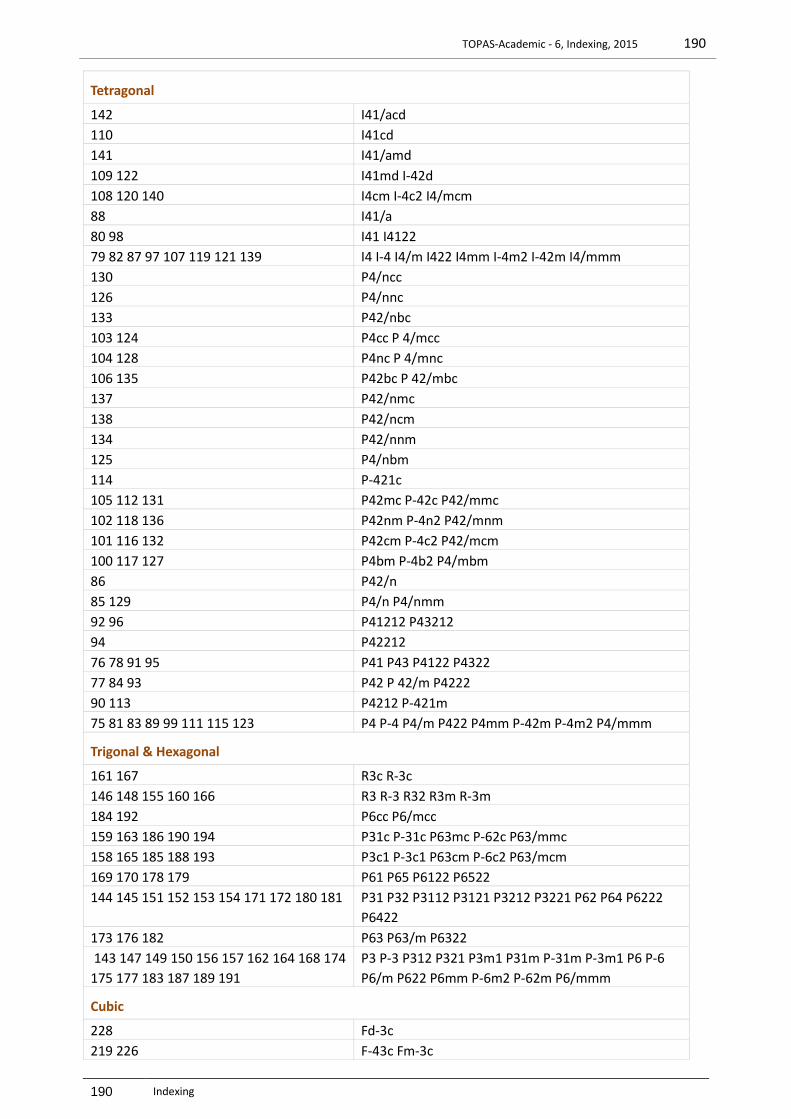
TOPAS-Academic - 6, Indexing, 2015 190
190 Indexing
Tetragonal
142 I41/acd
110 I41cd
141 I41/amd
109 122 I41md I-42d
108 120 140 I4cm I-4c2 I4/mcm
88 I41/a
80 98 I41 I4122
79 82 87 97 107 119 121 139 I4 I-4 I4/m I422 I4mm I-4m2 I-42m I4/mmm
130 P4/ncc
126 P4/nnc
133 P42/nbc
103 124 P4cc P 4/mcc
104 128 P4nc P 4/mnc
106 135 P42bc P 42/mbc
137 P42/nmc
138 P42/ncm
134 P42/nnm
125 P4/nbm
114 P-421c
105 112 131 P42mc P-42c P42/mmc
102 118 136 P42nm P-4n2 P42/mnm
101 116 132 P42cm P-4c2 P42/mcm
100 117 127 P4bm P-4b2 P4/mbm
86 P42/n
85 129 P4/n P4/nmm
92 96 P41212 P43212
94 P42212
76 78 91 95 P41 P43 P4122 P4322
77 84 93 P42 P 42/m P4222
90 113 P4212 P-421m
75 81 83 89 99 111 115 123 P4 P-4 P4/m P422 P4mm P-42m P-4m2 P4/mmm
Trigonal & Hexagonal
161 167 R3c R-3c
146 148 155 160 166 R3 R-3 R32 R3m R-3m
184 192 P6cc P6/mcc
159 163 186 190 194 P31c P-31c P63mc P-62c P63/mmc
158 165 185 188 193 P3c1 P-3c1 P63cm P-6c2 P63/mcm
169 170 178 179 P61 P65 P6122 P6522
144 145 151 152 153 154 171 172 180 181
P31 P32 P3112 P3121 P3212 P3221 P62 P64 P6222
P6422
173 176 182 P63 P63/m P6322
143 147 149 150 156 157 162 164 168 174
175 177 183 187 189 191
P3 P-3 P312 P321 P3m1 P31m P-31m P-3m1 P6 P-6
P6/m P622 P6mm P-6m2 P-62m P6/mmm
Cubic
228 Fd-3c
219 226 F-43c Fm-3c
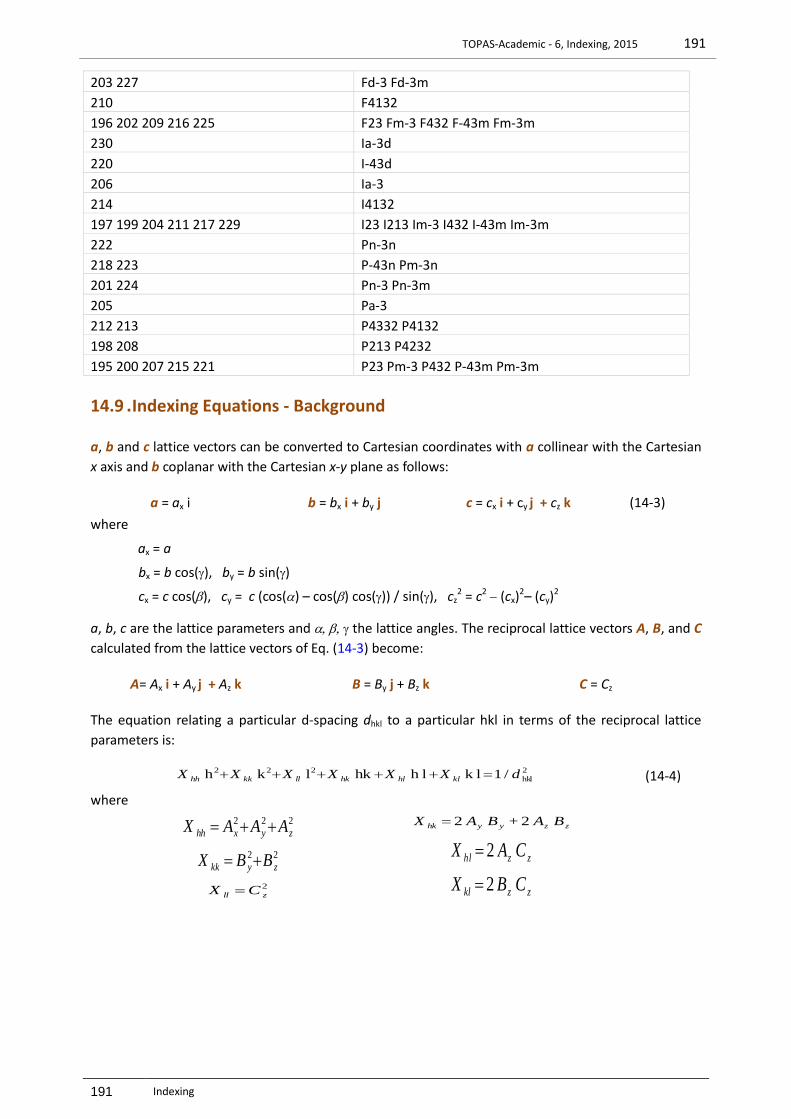
TOPAS-Academic - 6, Indexing, 2015 191
191 Indexing
203 227 Fd-3 Fd-3m
210 F4132
196 202 209 216 225 F23 Fm-3 F432 F-43m Fm-3m
230 Ia-3d
220 I-43d
206 Ia-3
214 I4132
197 199 204 211 217 229 I23 I213 Im-3 I432 I-43m Im-3m
222 Pn-3n
218 223 P-43n Pm-3n
201 224 Pn-3 Pn-3m
205 Pa-3
212 213 P4332 P4132
198 208 P213 P4232
195 200 207 215 221 P23 Pm-3 P432 P-43m Pm-3m
14.9 . Indexing Equations - Background
a, b and c lattice vectors can be converted to Cartesian coordinates with a collinear with the Cartesian
x axis and b coplanar with the Cartesian x-y plane as follows:
a = ax i b = bx i + by j c = cx i + cy j + cz k (14-3)
where
ax = a
bx = b cos(), by = b sin()
cx = c cos(), cy = c (cos() – cos() cos()) / sin(), cz2 = c2 (cx)
2– (cy)2
a, b, c are the lattice parameters and the lattice angles. The reciprocal lattice vectors A, B, and C
calculated from the lattice vectors of Eq. (14-3) become:
A= Ax i + Ay j + Az k B = By j + Bz k C = Cz
The equation relating a particular d-spacing dhkl to a particular hkl in terms of the reciprocal lattice
parameters is:
2
hkl
222 / 1 lk lh hk l k h dXXXXXX klhlhkllkkhh (14-4)
where
222 zyxhh AAAX
22 zykk BBX
2 zll CX
zzyyhk BABAX 2 + 2
zzhl CAX 2
zzkl CBX 2
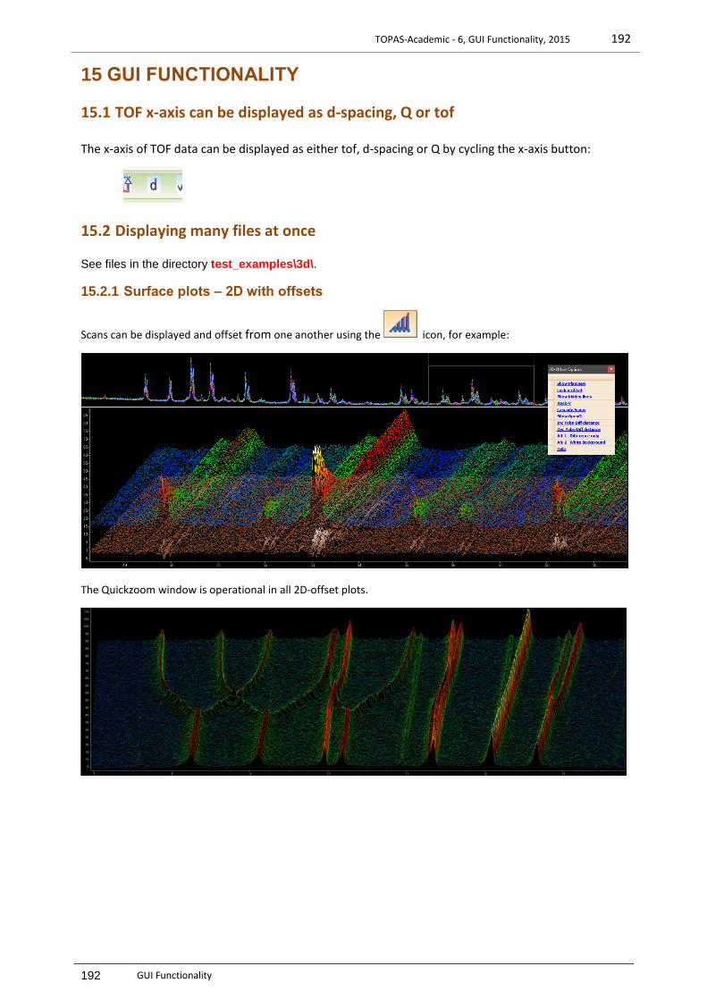
TOPAS-Academic - 6, GUI Functionality, 2015 192
192 GUI Functionality
15 GUI FUNCTIONALITY
15.1 TOF x-axis can be displayed as d-spacing, Q or tof
The x-axis of TOF data can be displayed as either tof, d-spacing or Q by cycling the x-axis button:
15.2 Displaying many files at once
See files in the directory test_examples\3d\.
15.2.1 Surface plots – 2D with offsets
Scans can be displayed and offset from one another using the icon, for example:
The Quickzoom window is operational in all 2D-offset plots.
13121110987
110
105
100
95
90
85
80
75
70
65
60
55
50
45
40
35
30
25
20
15
10
5
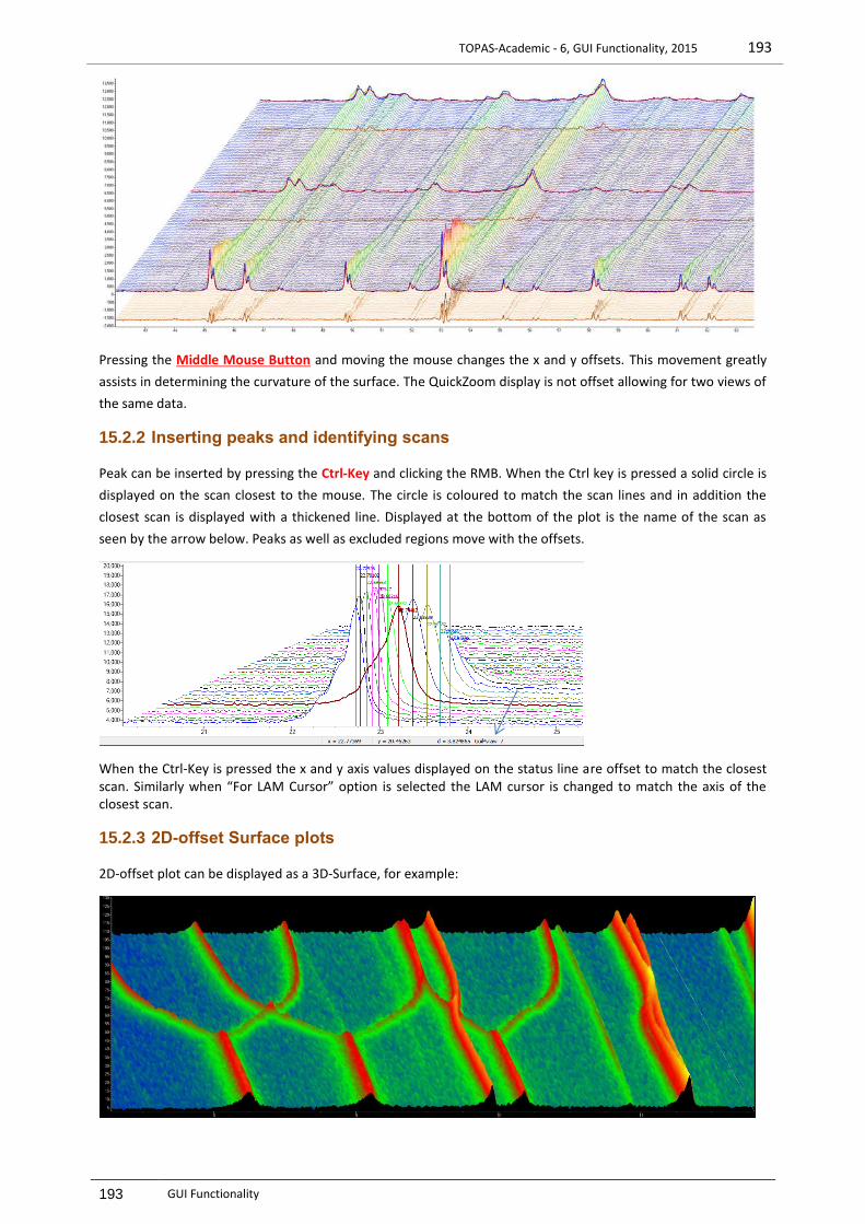
TOPAS-Academic - 6, GUI Functionality, 2015 193
193 GUI Functionality
Pressing the Middle Mouse Button and moving the mouse changes the x and y offsets. This movement greatly
assists in determining the curvature of the surface. The QuickZoom display is not offset allowing for two views of
the same data.
15.2.2 Inserting peaks and identifying scans
Peak can be inserted by pressing the Ctrl-Key and clicking the RMB. When the Ctrl key is pressed a solid circle is
displayed on the scan closest to the mouse. The circle is coloured to match the scan lines and in addition the
closest scan is displayed with a thickened line. Displayed at the bottom of the plot is the name of the scan as
seen by the arrow below. Peaks as well as excluded regions move with the offsets.
When the Ctrl-Key is pressed the x and y axis values displayed on the status line are offset to match the closest scan. Similarly when “For LAM Cursor” option is selected the LAM cursor is changed to match the axis of the closest scan.
15.2.3 2D-offset Surface plots
2D-offset plot can be displayed as a 3D-Surface, for example:
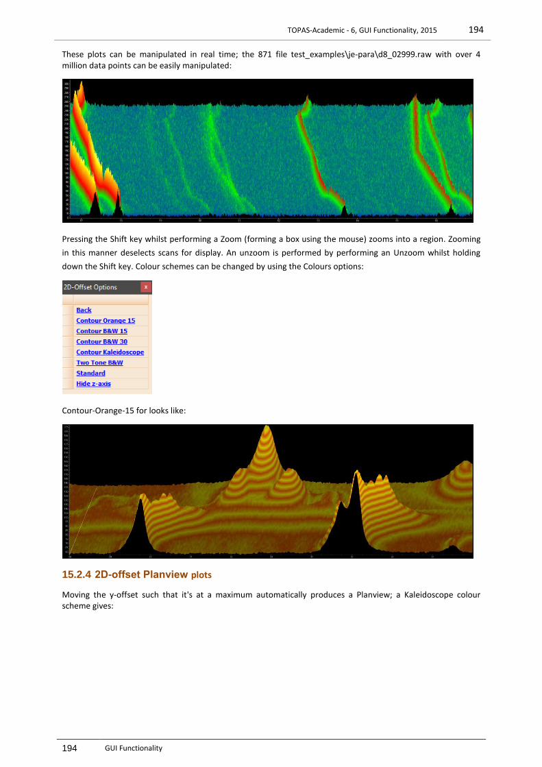
TOPAS-Academic - 6, GUI Functionality, 2015 194
194 GUI Functionality
These plots can be manipulated in real time; the 871 file test_examples\je-para\d8_02999.raw with over 4 million data points can be easily manipulated:
Pressing the Shift key whilst performing a Zoom (forming a box using the mouse) zooms into a region. Zooming
in this manner deselects scans for display. An unzoom is performed by performing an Unzoom whilst holding
down the Shift key. Colour schemes can be changed by using the Colours options:
Contour-Orange-15 for looks like:
15.2.4 2D-offset Planview plots
Moving the y-offset such that it's at a maximum automatically produces a Planview; a Kaleidoscope colour scheme gives:

TOPAS-Academic - 6, GUI Functionality, 2015 195
195 GUI Functionality
The Standard colour scheme gives:
Zooming gives:
Planview can also have x-axis offsets with line scans overlain:
989694929088868482807876747270686664626058565452504846444240383634323028262422201816141210
2,700
2,600
2,500
2,400
2,300
2,200
2,100
2,000
1,900
1,800
1,700
1,600
1,500
1,400
1,300
1,200
1,100
1,000
900
800
700
600
500
400
300
200
100
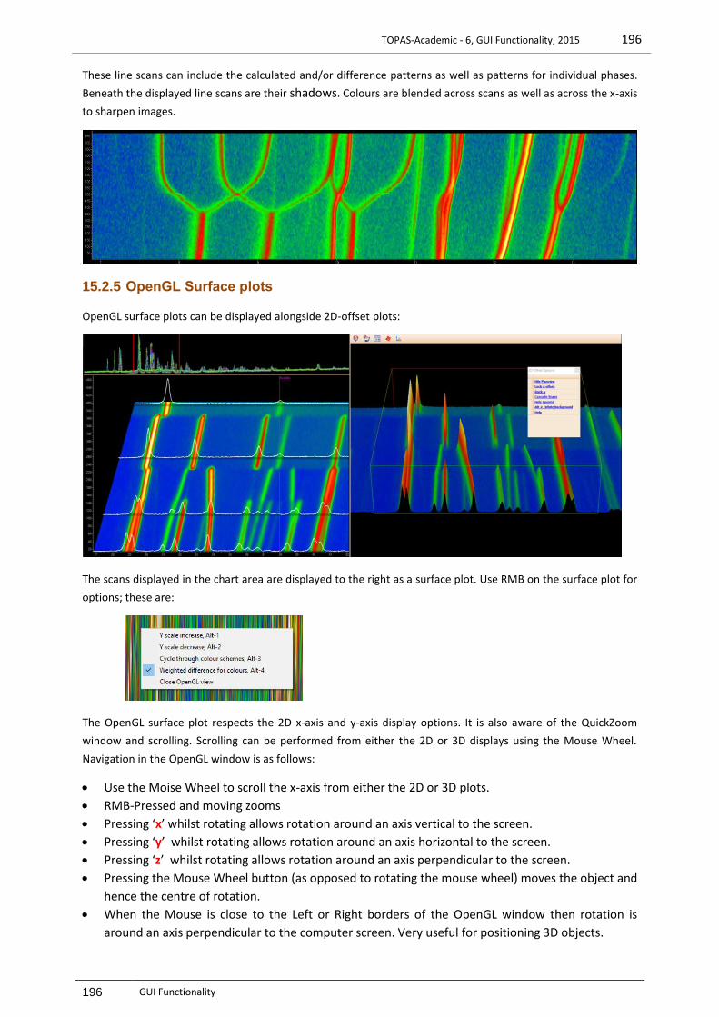
TOPAS-Academic - 6, GUI Functionality, 2015 196
196 GUI Functionality
These line scans can include the calculated and/or difference patterns as well as patterns for individual phases.
Beneath the displayed line scans are their shadows. Colours are blended across scans as well as across the x-axis
to sharpen images.
15.2.5 OpenGL Surface plots
OpenGL surface plots can be displayed alongside 2D-offset plots:
The scans displayed in the chart area are displayed to the right as a surface plot. Use RMB on the surface plot for
options; these are:
The OpenGL surface plot respects the 2D x-axis and y-axis display options. It is also aware of the QuickZoom
window and scrolling. Scrolling can be performed from either the 2D or 3D displays using the Mouse Wheel.
Navigation in the OpenGL window is as follows:
Use the Moise Wheel to scroll the x-axis from either the 2D or 3D plots.
RMB-Pressed and moving zooms
Pressing ‘x’ whilst rotating allows rotation around an axis vertical to the screen.
Pressing ‘y’ whilst rotating allows rotation around an axis horizontal to the screen.
Pressing ‘z’ whilst rotating allows rotation around an axis perpendicular to the screen.
Pressing the Mouse Wheel button (as opposed to rotating the mouse wheel) moves the object and
hence the centre of rotation.
When the Mouse is close to the Left or Right borders of the OpenGL window then rotation is
around an axis perpendicular to the computer screen. Very useful for positioning 3D objects.
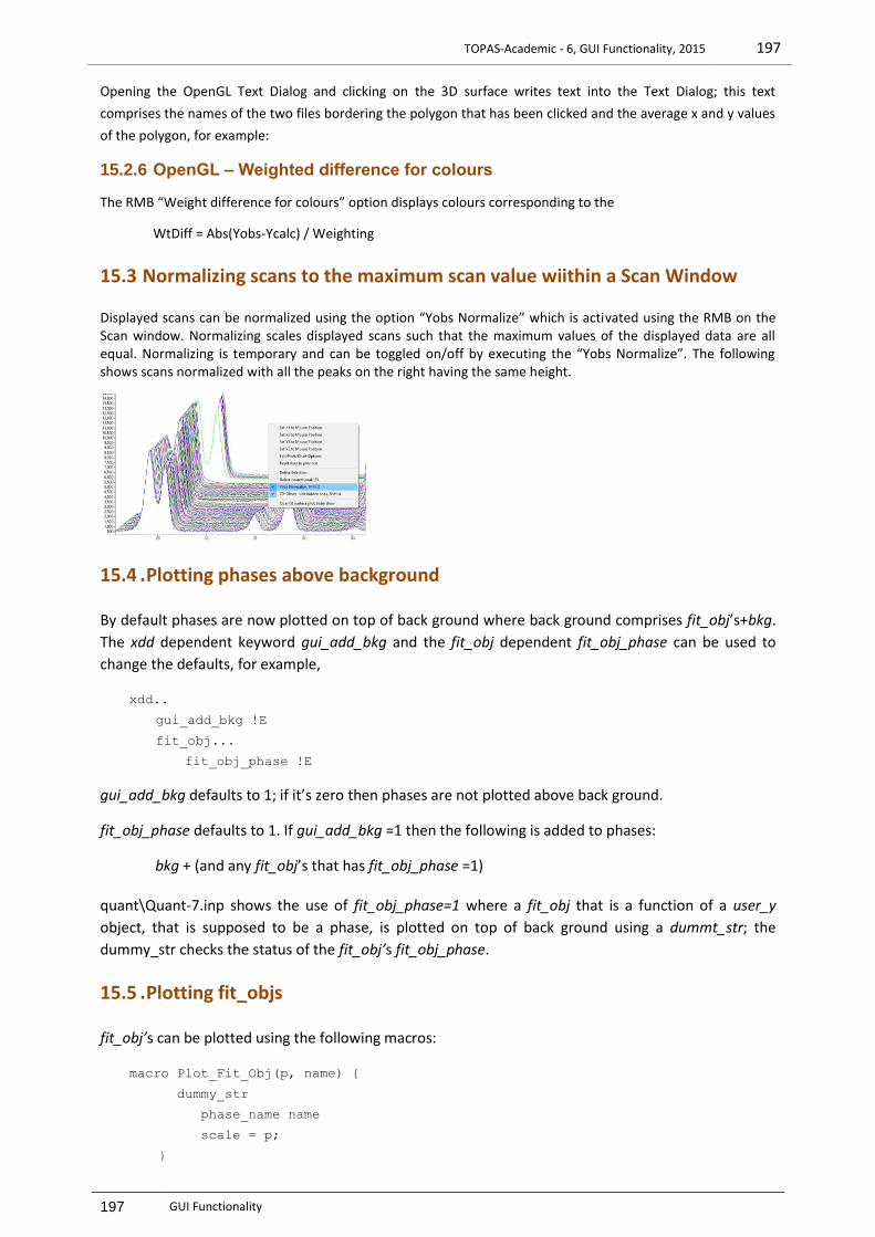
TOPAS-Academic - 6, GUI Functionality, 2015 197
197 GUI Functionality
Opening the OpenGL Text Dialog and clicking on the 3D surface writes text into the Text Dialog; this text
comprises the names of the two files bordering the polygon that has been clicked and the average x and y values
of the polygon, for example:
15.2.6 OpenGL – Weighted difference for colours
The RMB “Weight difference for colours” option displays colours corresponding to the
WtDiff = Abs(Yobs-Ycalc) / Weighting
15.3 Normalizing scans to the maximum scan value wiithin a Scan Window
Displayed scans can be normalized using the option “Yobs Normalize” which is activated using the RMB on the Scan window. Normalizing scales displayed scans such that the maximum values of the displayed data are all equal. Normalizing is temporary and can be toggled on/off by executing the “Yobs Normalize”. The following shows scans normalized with all the peaks on the right having the same height.
15.4 . Plotting phases above background
By default phases are now plotted on top of back ground where back ground comprises fit_obj’s+bkg.
The xdd dependent keyword gui_add_bkg and the fit_obj dependent fit_obj_phase can be used to
change the defaults, for example,
xdd..
gui_add_bkg !E
fit_obj...
fit_obj_phase !E
gui_add_bkg defaults to 1; if it’s zero then phases are not plotted above back ground.
fit_obj_phase defaults to 1. If gui_add_bkg =1 then the following is added to phases:
bkg + (and any fit_obj’s that has fit_obj_phase =1)
quant\Quant-7.inp shows the use of fit_obj_phase=1 where a fit_obj that is a function of a user_y
object, that is supposed to be a phase, is plotted on top of back ground using a dummt_str; the
dummy_str checks the status of the fit_obj’s fit_obj_phase.
15.5 . Plotting fit_objs
fit_obj’s can be plotted using the following macros:
macro Plot_Fit_Obj(p, name) {
dummy_str
phase_name name
scale = p;
}
TOPAS-Academic - 6, GUI Functionality, 2015 198
198 GUI Functionality
macro Plot_Fit_Obj(name) {
dummy_str
phase_name name
}
See test_examples\voigt-approx\fit-obj.inp for example; ie.
xdd...
fit_obj !f1 = ...
Plot_Fit_Obj(f1, “Fit Obj”)
Plotting is via a dummy_str and the scale parameter of the dummy_str is set to the name given to the
fit_obj, which in this case is f1. At the plotting stage the dummy_str borrows the calculated pattern
from the fit_obj.
The scale parameter of the dummy_str has some intelligence built into it such that if scale is not a
function of a fit_obj name then it will search the place of the item it is a function of for a calculated
pattern. For example, in the following:
xdd...
Plot_Fit_Obj(a, “Fit Obj”)
fit_obj = a ...
prm a ...
the ‘a’ parameter lives locally to the fit_obj as it is defined after the fit_obj. Defining the scale
parameter of the dummy_str in terms of ‘a’ therefore allows the dummy_str to determine where to
find the calculated pattern to display. In this way macros such as the PV macro can be used and
plotted without having to define a name for the fit_obj, see test_examples\pvs.inp. Sometimes the
fit_obj has no name and no parameter that belongs to it; instead of naming the fit_obj or rearranging
prm definitions the second Plot_Fit_Obj macro can be used:
xdd...
fit_obj =
Plot_Fit_Obj(“plot previously defined fit_obj”)
Here the fit_obj defined prior to Plot_Fit_Obj is plotted.

TOPAS-Academic - 6, GUI Functionality, 2015 199
199 GUI Functionality
15.6 .. Display of Normalized SigmaYobs^2
Useful for checking SigmaYobs anomalies from VCT or XYE files; here’s an example :
The normalization is as follows:
SigmaYobs^2 displayed = SigmaYobs^2 Sum[ Yobs ] / Sum[ SigmaYobs^2]
This puts the display of SigmaYobs^2 on a similar scale to Yobs. For normal x-ray data
SigmaYobs=Sqrt(Yobs) and hence nothing is done as the displayed plot would simply be equal to Yobs.
On some data sets, TOF for example, the magnitude of SigmaYobs can be small; thus when refining on
multiple data sets from different sources the weighting schemes may need to be modified in order to
give the desired weight to the data sets. The option for display is as follows::

TOPAS-Academic - 6, GUI Functionality, 2015 200
200 GUI Functionality
15.7 .. Cumulative Chi2
A kernel operation that results in the following graphical display:
Uses the weighting from the kernel which can be user defined or otherwise.
SigmaYobs is used in the weighting if it exists.
Prior to graphical display it is scaled to have the same maximum intensity as the maximum of Yobs.
Data is obtained from the kernel and thus excluded regions are ignored as shown in the plot above.
Tabs for Cumulative Chi2 has been included in the appropriate GUI tabs as seen in the following:
14013012011010090807060504030
55,000
50,000
45,000
40,000
35,000
30,000
25,000
20,000
15,000
10,000
5,000
0
-5,000
-10,000
-15,000
-20,000
Structure 100.00 %

TOPAS-Academic - 6, GUI Functionality, 2015 201
201 GUI Functionality
15.8 .. Correlation Matrix display
A Correlation matrix window activated from the Fit Dialog; it operates in Launch or GUI modes.
Example output is as follows:
Both the A-matrix and the correlation matrix include penalties/restraints depending on whether
do_errors_include_penalties and/or do_errors_include_restraints are defined. The display of the
matrix can be zoomed using Ctrl-MouseWheel, for example:
MouseMove over the correlation matrix displays a Hint comprising the corresponding parameter
names, values and errors. Left Mouse button down and dragging translates the matrix.

TOPAS-Academic - 6, GUI Functionality, 2015 202
202 GUI Functionality
15.9 . Fading a structure
The intensity of atom colours displayed in OpenGL can be adjusted using the Fade spin button of the
OpenGL options grid; for example:
15.10 Normals Plot
An OpenGL plot of lattice plane Normals with the lengths of the Normals defined by the keyword
normals_plot. For example:
normals_plot = Abs(H * K + L^2) + 1;
normals_plot_min_d .3
normals_plot_min_d is optional; small values (ie. 0.1) could lead to millions of points and users could
blow up their computers. Here’s some output from the test example CLAY.INP:

TOPAS-Academic - 6, GUI Functionality, 2015 203
203 GUI Functionality
The slider in the plot is activated by clicking on the button. This slider multiplies the length of
the normals_plot equation before generating the surface. The exact formulation for the
multiplications is as follows.
Definitions:
s = the multiplier which has a value (not shown to the user) that varies between 0 and 1.
N = the diffraction vector directions with lengths as given by the normals_plot equation.
N = Sqrt(N . N) = magnitude of N
Nmax = maximum N
Before generating the shape N is multiplied by:
For s < 0.25: ((N / Nmax)^(4*s)) * Nmax / N
For 0.25 <= s < 0.5: ((N / Nmax)^(4*(0.5-s))) * Nmax / N
For 0.5 < s <= 0.75: (4*(0.5-s)) * Nmax / N + (1-s)
For 0.75 < s <= 1: (((4*(0.75-s)) + Nmax / N
15.11 Improvements to the Grid
Data can now be sorted by Double Clicking on Column Headings. Sorting alternates between
ascending and descending order. On leaving a particular grid the column most recently sorted is
remembered. On re-entry of that particular grid the data is again sorted according to the saved state.
A small < or > sign is displayed to the left of the Column heading name. Sorting works for all grids that

TOPAS-Academic - 6, GUI Functionality, 2015 204
204 GUI Functionality
display data with rows that are similar in Type; ie. Peak data, sites etc…. Val and Error columns are
sorted numerically. Hkls, F^2 and other obvious numeric columns are also sorted numerically.
However, Min and Max are sorted using strings as they can be equations and hence their fields are
strings.
CTRL-MouseWheel zooms/un-zooms the text of a grid
MouseDownMouseMove for Panning.
15.12 Mouse operation in OpenGL Graphics
First some definitions
LMB = Left Mouse Button
RMB = Right Mouse Button
MID = Mouse Wheel or Middle button on Laptops
MM = Mouse Moving
WM = Wheel moving
LMB-D = Left Mouse Button Down
RMB-D = Right Mouse Button Down
MW-D = Mouse Wheel Down
For example, LMB-D- MM is simply dragging with the LMD
Image rotation/translation operations are:
LMB-D- MM rotates the image.
LMB-D- MM and quick release initiates continuous rotation.
LMD-D-MM on the first 10% of the viewport from the left or the last 10% from the right rotates
around an axis perpendicular to the screen. This is another way of doing what Shift-LMB-D-MM
does but without the need for keyboard input. 10% seems a good amount as it does not seem to
interfere with normal rotation.
MW zooms in addition to the usual RMB-D-MM.
MID-D-MM translates the image in the plane of the screen.
Images are rotated around the centre of gravity (or centre of unit cell) unless there’s a change using
the RMB-D options.

TOPAS-Academic - 6, References, 2015 205
205 References
16 REFERENCES
Ainsworth, C. M.; Lewis, J. W.; Wang, C.; Johnstone, H. E.; Mendhis, B. G.; Brand, H. E. A.; Coelho, A.
A.; Evans, J. S. O. (2016). Chem. Mater., 28, 3184–3195. “3D Transition Metal Ordering and
Rietveld Stacking Fault Quantification in the New Oxychalcogenides La2O2Cu2–4xCd2xSe2”
Baerlocher, C; Gramm, F.; Massüger, L; McCusker, L; He, Z; Hovmöller, S & Zou, X. (2007). SCIENCE
VOL 315 23 FEBRUARY 2007
Baerlocher, C.; McCusker, L.B.; & Palatinus, L. (2007). Z. Kristallogr. 222, 47-53
Balzar, D. (1999). Microstructure Analysis from Diffraction, edited by R. L. Snyder, H. J. Bunge, and J.
Fiala, International Union of Crystallography, 1999. “Voigt-function model in diffraction line-
broadening analysis”
Bergmann, J., Kleeberg, R., Haase, A. & Breidenstein, B. (2000). Mat. Sci. Forum, 347-349, 303-308.
“Advanced Fundamental Parameters Model for Improved Profile Analysis”.
Brindley, G.W. (1945). Phil. Mag., 36, 347-369. “The effect of grain or particle size on X-ray reflections
from mixed powders and alloys, considered in relation to the quantitative determination of
crystalline substances by X-ray methods”
Broyden, C.G., J. Inst. Maths. Applics., Vol. 6, pp 76-90, 1970. "The Convergence of a Class of Double-
rank Minimization Algorithms"
Cagliotti, G., Paoletti, A. & Ricci, F.P (1958). Nucl. Inst., 3, 223-228. “Choice of collimators for a crystal
spectrometer for neutron diffraction”
Cheary, R. W. & Coelho, A. (1992). J. Appl. Cryst. 25, 109-121. “A fundamental parameters approach
to X-ray line-profile fitting”
Cheary, R.W. & Coelho, A.A. (1994). J. Appl. Cryst., 27 (5), 673-681. “Synthesizing and fitting linear
position-sensitive detector step-scanned line profiles”
Cheary, R.W. & Coelho, A.A. (1998a). J. Appl. Cryst., 31, 851-861. “Axial divergence in a conventional
X-ray powder diffractometer I. Theoretical foundations”
Cheary, R.W. & Coelho, A.A. (1998b). J. Appl. Cryst., 31, 862-868. “Axial divergence in a conventional
X-ray powder diffractometer II. Implementation and comparison with experiment”
Cheary, R. W.; Coelho, A. A. and Cline, J. P. (2004). Journal of Research-National Institute of Standards
and Technology 109 (2004): 1-26. "Fundamental parameters line profile fitting in laboratory
diffractometers"
Coelho, A. A. & Cheary, R. W. (1997). Computer Physics Communications, 104, 15-22. “A fast and
simple method for calculating electrostatic potentials”
Coelho, A. A., (2000). J. Appl. Cryst., 33, Part 3 Number 2, "Structure Solution by Simulated Annealing"
Coelho, A. A., (2003). J. Appl. Cryst., 36, 86–95. “Indexing of powder diffraction patterns by iterative
use of singular value decomposition”.
Coelho, A. A. (2005). J. Appl. Cryst. 38, 455-461. "A bound constrained conjugate gradient solution
method as applied to crystallographic refinement problems"

TOPAS-Academic - 6, References, 2015 206
206 References
Coelho, A. A. (2007). Acta Cryst., A36, 400–406. “A charge-flipping algorithm incorporating the
tangent formula for solving difficult structures”
Coelho, A. A; Evans, J.; Evans, I; Kern, A.; Parsons, S. (2011). Powder Diffraction, Vol. 26 Number 4
sup, "The TOPAS symbolic computation system"
Coelho, A. A.; Chater, P.A.; Kern, A. (2015). J. Appl. Cryst. (2015). 48, Volume 48, Part 3, 869-875.
“Fast synthesis and refinement of the atomic pair distribution function”
Baerlocher, C; Gramm, F.; Massüger, L; McCusker, L; He, Z; Hovmöller, S & Zou, X. (2007). SCIENCE
VOL 315 23 FEBRUARY 2007.
Chernick, M.R. (1999). Bootstrap Methods, A Practitioner’s Guide, Wiley, New York.
David, W.I.F; Matteo, L.; Scardi, P. (2010). Materials Science Forum Vol. 651 pp 187-200
DiCiccio, T.J. & Efron, B. (1996). Bootstrap confidence intervals (with discussion), Statistical Science
11, 189–228.
Durbin, J. & Watson, G.S. (1971). Biometrika, 58, 1-19. “Testing for Serial Correlation in Least Square
Regression, III”
Efron, B. & Tibshirani, R. (1986). Bootstrap methods for standard errors, confidence intervals and
other measures of statistical accuracy, Statistical Science 1, 54–77.
Fletcher, R. (1970). Computer Journal, Vol. 13, pp 317-322. "A New Approach to Variable Metric
Algorithms"
Finger, L.W., Cox, D.E & Jephcoat, A.P. (1994). J. Appl. Cryst., 27, 892-900. “A correction for powder
diffraction peak asymmetry due to axial divergence”
Flack, H. D. (1983). Acta Cryst. A39, 876-881
Goldfarb, D. (1970). Mathematics of Computing, Vol. 24, pp 23-26. “A Family of Variable Metric
Updates Derived by Variational Means”
Hauptman, H. & Karle, J. (1956). Acta Cryst. 9, 635
Hill, R.J. & Flack, H.D. (1987). J. Appl. Cryst., 20, 356-361. “The Use of the Durbin-Watson d Statistic in
Rietveld Analysis”
Hölzer, G., Fritsch, M., Deutsch, M., Härtwig, J. & Förster, E. (1997). Physical Review A, 56, 4554-4568.
“K1,2 and K1,2 X-ray emission lines of the 3d transition metals”
Järvinen, M. (1993). J. Appl. Cryst., 26, 525-531. “Application of symmetrized harmonics expansion to
correction of the preferred orientation effect”
Johnson, C.K. & Levy, H.A. (1974). International Tables for X-ray Crystallography, IV, 311 - 336.
“Thermal-motion analysis using Bragg diffraction data”
Kopp, Joachim. (2006). Int.J.Mod.Phys.C19:523-548,2008
Leoni, M.; Di Maggio, R.; Polizzi, S; Scardi P. (2004), J. Am. Ceram. Soc. 87, 1133-1140.
Le Bail, A. & Jouanneaux, A. (1997). J. Appl. Cryst., 30, 265-271. “A Qualitative Account for Anisotropic
Broadening in Whole-Powder-Diffraction-Pattern Fitting by Second-Rank Tensors”

TOPAS-Academic - 6, References, 2015 207
207 References
Lister, S. E.; Radosavljevic Evans, I.; Howard, J. A. K.; Coelho A. and Evans, J. S. O. (2004). Chemical
Communications, Issue 22.
March, A. (1932). Z. Krist., 81, 285-297. “Mathematische Theorie der Regelung nach der Korngestalt
bei affiner Deformation”
Markvardsen, A. J.; David, W. I. F.; Johnston, J. and Shankland K. (2001), Acta Cryst. A57, 47
Marquardt, D. W. (1963). J. Soc. Ind. Appl. Math., 11(2), 431-331. “An algorythm for least-squares
estimation of nonlinear parameters”
O'Connor, B.H.; and Raven, M. D. (1988). Powder Diffraction, Vol. 3, No. 1. "Application of the Rietveld
Refinement Procedure in Assaying Powdered Mixtures"
Oszlányi, G. & Süto A. (2004). Acta Cryst. A60, 134-141
Oszlányi, G. & Süto A. (2005). Acta Cryst. A61, 147-152
Oszlányi, G. & Süto A. (2006). Acta Cryst. A63, 156–163
Oszlányi, G.; Süto A.; Czugler, M. & Parkanyi, L. (2006). J. AM. CHEM. SOC. 9 VOL. 128, NO. 26, 8393.
“Charge Flipping at Work: A Case of Pseudosymmetry”.
Scardi, P. & Leoni, M. (2001). Acta Cryst. A 57, 604-613.
Shanno, D.F. (1970). Mathematics of Computing, Vol. 24, pp 647-656. "Conditioning of Quasi-Newton
Methods for Function Minimization"
Favre-Nicolin, V. and Cerny, R. (2002) EPDIC 8 proceedings. “Fox: Modular Approach to Crystal
Structure Determination from Powder Diffraction”
Sabine, T. M., Hunter, B. A., Sabine, W. R., Ball, C. J. (1998): J. Appl. Cryst. 31, 47-51
Schneider, T. R. & Sheldrick, G. M. (2002). Acta Cryst. D58, 1772-1779. “Substructure solution with
SHELXD“
Shiono, M. & Woolfson, M. M. (1992). Acta Cryst. A48, 451-456
Whitfield, P. S. and Coelho, A. A. (2016). J. Appl. Cryst. (2016). 49, doi:10.1107/S1600576716011961.
"Asymmetric band flipping for time-of-flight neutron diffraction data".
Young, R.A. (1993). The Rietveld Method, edited by R.A. Young, IUCr Book Series, Oxford University
Press 1993, 1-39. “Introduction to the Rietveld method”