Technical note: Characterising and comparing different ...

Clim. Past, 17, 545–563, 2021https://doi.org/10.5194/cp-17-545-2021© Author(s) 2021. This work is distributed underthe Creative Commons Attribution 4.0 License.

Technical note: Characterising and comparing differentpalaeoclimates with dynamical systems theoryGabriele Messori1,2,3,4 and Davide Faranda5,6,7

1Department of Earth Sciences, Uppsala University, Uppsala, Sweden2Centre of Natural Hazards and Disaster Science (CNDS), Uppsala University, Uppsala, Sweden3Department of Meteorology, Stockholm University, Stockholm, Sweden4Bolin Centre for Climate Research, Stockholm University, Stockholm, Sweden5Laboratoire des Sciences du Climat et de l’Environnement, LSCE/IPSL, CEA-CNRS-UVSQ,Université Paris-Saclay, Gif-sur-Yvette, France6London Mathematical Laboratory, London, UK7LMD/IPSL, Ecole Normale Superieure, PSL research University, Paris, France

Correspondence: Gabriele Messori ([email protected])

Received: 30 July 2020 – Discussion started: 27 August 2020Revised: 7 January 2021 – Accepted: 10 January 2021 – Published: 2 March 2021

Abstract. Numerical climate simulations produce vastamounts of high-resolution data. This poses new challengesto the palaeoclimate community – and indeed to the broaderclimate community – in how to efficiently process and inter-pret model output. The palaeoclimate community also facesthe additional challenge of having to characterise and com-pare a much broader range of climates than encountered inother subfields of climate science. Here we propose an analy-sis framework, grounded in dynamical systems theory, whichmay contribute to overcoming these challenges. The frame-work enables the characterisation of the dynamics of a givenclimate through a small number of metrics. These may beapplied to individual climate variables or to several variablesat once, and they can diagnose properties such as persis-tence, active number of degrees of freedom and coupling.Crucially, the metrics provide information on instantaneousstates of the chosen variable(s). To illustrate the framework’sapplicability, we analyse three numerical simulations of mid-Holocene climates over North Africa under different bound-ary conditions. We find that the three simulations produceclimate systems with different dynamical properties, such aspersistence of the spatial precipitation patterns and couplingbetween precipitation and large-scale sea level pressure pat-terns, which are reflected in the dynamical systems metrics.We conclude that the dynamical systems framework holdssignificant potential for analysing palaeoclimate simulations.

At the same time, an appraisal of the framework’s limitationssuggests that it should be viewed as a complement to moreconventional analyses, rather than as a wholesale substitute.

1 Motivation

Numerical climate models have enjoyed widespread usein palaeoclimate studies, from early investigations basedon simple thermodynamic or general circulation models(e.g. Gates, 1976; Donn and Shaw, 1977; Barron et al.,1980) to the state-of-the-art models being used in the fourthphase of the Paleoclimate Modelling Intercomparison Project(PMIP4, Kageyama et al., 2018). Compared to data frompalaeo-archives, which are typically geographically sparseand with a low temporal resolution even for the more re-cent palaeoclimates (e.g. Bartlein et al., 2011), numericalclimate simulations produce a vast amount of horizontallygridded, vertically resolved data with a high temporal reso-lution. Moreover, the resolution and complexity of numericalmodels – and hence the amount of data they produce – hasincreased vastly in recent years. This poses new challengesto the palaeoclimate community in how to efficiently processand interpret model output – indeed an issue that is faced bythe broader climate community (Schnase et al., 2016).

Published by Copernicus Publications on behalf of the European Geosciences Union.

546 G. Messori and D. Faranda: Comparing palaeoclimates with dynamical systems

A related, yet distinct, challenge faced by the palaeocli-mate community are the large uncertainties often found inpalaeo-simulations. These reflect the uncertainties in palaeo-archives and in our knowledge of the boundary conditionsand forcings affecting past climates (e.g. Kageyama et al.,2018). Thus, different simulations of the climate in the sameperiod and region may yield very different results. Thisemerges in both reconstructions of climates from millionsof years ago, such as the mid-Pliocene warm period over3 Ma BP (e.g. Haywood et al., 2013) and in climates muchcloser to us, such as the mid-Holocene around 6000 years BP(e.g. Pausata et al., 2016). Characterising and understandingthese discrepancies requires analysis tools that can efficientlydistil the differences between the simulated palaeoclimates.

Here, we propose an analysis framework which addressesthe challenges of efficiently processing and interpreting largeamounts of model output to compare different simulatedpalaeoclimates. The framework is grounded in dynamicalsystems theory and enables the characterisation of the dy-namics of a given dynamical system – for example the at-mosphere – through three one-dimensional metrics. The firstmetric estimates the persistence of instantaneous states of thesystem. We term this metric rather mundanely “persistence”.The second metric, which we term “local dimension”, pro-vides information on how the system evolves to or from in-stantaneous states. Finally, the co-recurrence ratio is a metricapplicable to two (or more) variables, which quantifies theirinstantaneous coupling. In other words, the dynamical infor-mation embedded in three-dimensional (latitude, longitudeand time) or four-dimensional (latitude, longitude, pressurelevel and time) data, commonly produced by climate mod-els, can be projected onto three metrics, which each providea single value for every time step in the data. These may thenbe interpreted and compared with relative ease.

The rest of this technical note is structured as follows: inSect. 2 we briefly describe the theory underlying the dynam-ical systems framework, and provide both a qualitative and atechnical description of the metrics. We further provide a linkto a repository from which MATLAB code to implement themetrics may be obtained. In Sect. 3, we illustrate the appli-cation of the metrics to palaeoclimate data and their interpre-tation by using a set of recent numerical simulations for themid-Holocene climate in North Africa. This is not meant tobe a comprehensive analysis but instead provides the flavourof the information provided by our framework. We concludein Sect. 4 by reflecting on the framework’s strengths andlimitations and by outlining potential applications in futurepalaeoclimate studies.

2 A qualitative overview and theoreticalunderpinnings of the dynamical systemsframework

In Sect. 2.1, we explain qualitatively how the dynamical sys-tems metrics we use may be interpreted when computed fora hypothetical sea level pressure (SLP) field. We also pro-vide a conceptual analogy to raindrops flowing on complextopography. In Sect. 2.2, we provide a brief mathematicalderivation of the metrics and outline some of the obstaclesencountered when computing them for climate data.

2.1 A qualitative overview of the dynamical systemsframework

The dynamical systems framework we propose rests on threeindicators. All are instantaneous in time, meaning that givena long data series, they provide a value for each time step.For example, if we were to analyse daily latitude–longitudeSLP in a given geographical region over 30 years, we wouldhave 30× 365 values for each indicator.

The first indicator, termed “local dimension” (d), providesa proxy for the number of active degrees of freedom of thesystem about a state of interest (Lucarini et al., 2016; Farandaet al., 2017a). In other words, the value of d for a given day inour SLP dataset tells us how the SLP in the chosen geograph-ical region can evolve to or from the pattern it displays onthat day. The number of different possible evolutions is pro-portional to the number of degrees of freedom, and thereforedays with a low (high) local dimension correspond to SLPpatterns that derive from and may evolve into a small (large)number of other SLP patterns in the preceding and followingdays. An intuitive – if not entirely precise – analogy may bedrawn with the path followed by raindrops once they fall tothe ground (Fig. A1a). In this case, an impermeable topogra-phy would effectively function as a bi-dimensional potentialsurface. If there is a deep valley, all raindrops falling on asmall patch of ground on the side of the valley will followsimilar paths: they will all reach the bottom of the valley andthen flow along it. There may be places where the drops canfollow slightly different paths, for example in going arounda large stone, but their general course is constrained. Thiswould be equivalent to a patch of ground with a low localdimension. Now imagine the case of raindrops falling ona second small patch of ground, but this time on a craggymountain peak. In the latter case, very small changes in ex-actly where each drop falls may result in the drops followingcompletely different paths. A first drop may follow a narrowcrevasse to the side of the patch, while a second drop fallingvery close to it may take an entirely different route towardsthe bottom of the valley. This would be equivalent to havinga high local dimension.

The second indicator, termed “persistence” (θ−1), mea-sures the mean residence time of the system around a givenstate. In other words, if a given day in our SLP dataset

Clim. Past, 17, 545–563, 2021 https://doi.org/10.5194/cp-17-545-2021

G. Messori and D. Faranda: Comparing palaeoclimates with dynamical systems 547

has a high (low) persistence, the SLP pattern on that dayhas evolved slowly (rapidly) from and will evolve slowly(rapidly) to a different SLP pattern. The higher the persis-tence, the more likely it is that the SLP patterns on the daysimmediately preceding and following the chosen day will re-semble the SLP pattern of that day. This metric is relatedto, yet distinct from, the notion of persistence issuing fromweather regimes and similar partitionings of the atmosphericvariability (Hochman et al., 2019, 2020b). Returning to ourraindrop analogy (Fig. A1b), one may imagine that if the val-ley’s sides are steep, the raindrops will leave the patch ofground they have fallen on very rapidly, i.e. a low persis-tence. If, on the other hand, the valley is edged by shallowslopes, the raindrops will take longer to leave the patch, i.e.a high persistence.

Both indicators may be used to characterise the dynamicsunderlying complex systems, including the Earth’s climate(e.g. Faranda et al., 2017a; Buschow and Friederichs, 2018;Brunetti et al., 2019; Gualandi et al., 2020; Hochman et al.,2020a). On a more practical level, they can also be linked tothe notion of intrinsic predictability of the system’s differentstates. A state with a low d and high θ−1 will afford a bet-ter predictability than one with a high d and low θ−1. Formore detailed discussions on this topic and a comparison tothe conventional idea of predictability as evaluated throughnumerical weather forecasts, see Messori et al. (2017), Scherand Messori (2018), and Faranda et al. (2019a). Both d andθ−1 may in principle be computed for more than one cli-mate variable jointly (Faranda et al., 2020; De Luca et al.,2020b, a), but here we will focus on their univariate imple-mentation.

Unlike the first two, the third metric we propose here,termed “co-recurrence ratio” (α), is exclusively defined fortwo or more variables. Given two climate variables, α di-agnoses the extent to which their recurrences co-occur andhence provides a measure of the coupling between them(Faranda et al., 2020). As an example, imagine that we nowhave both our SLP dataset and a corresponding precipita-tion dataset, which also provides daily values on a latitude–longitude grid. If α on a given day is large, then every timewe have an SLP pattern on another day that closely resemblesthe SLP pattern of the chosen day (i.e. a “recurrence”), theprecipitation pattern on that other day will also resemble theprecipitation pattern of the chosen day. In other words, recur-rences of similar SLP patterns lead to recurrences of similarprecipitation patterns, which would suggest that the two vari-ables are highly coupled. If α on a given day is small, then ev-ery time we have an SLP pattern on another day that closelyresembles the SLP pattern of the chosen day, the precipitationpattern on that other day will not resemble the precipitationpattern of the chosen day. In other words, recurrences of sim-ilar SLP patterns do not lead to recurrences of similar precip-itation patterns, which would suggest that the two variablesare weakly coupled. We note that α may not be interpretedin terms of causation. However, since the joint recurrence of

two fields implies the existence of common underlying dy-namics, the information it provides is nonetheless groundedin the physics of the system being analysed. Finally, α pro-vides very different information from many other conven-tional statistical dependence measures, since it gives a valuefor every time step in the dataset. In our raindrop analogy,α could link the raindrop paths to, for example, the growthpattern of vegetation on the ground (Fig. A1c, d). Vegeta-tion will affect the raindrop paths, yet the path of the rain-drops will determine where the water flows and hence affectthe growth of the vegetation. One may therefore imagine thatwhenever the raindrops collectively follow similar paths, thiswill correspond to a recurring pattern of vegetation growth.Conversely, whenever there are similar patterns of vegetationgrowth, this will presumably result in the raindrops follow-ing similar paths. The raindrop paths and vegetation growthpatterns therefore co-recur, resulting in a high α.

2.2 Theoretical underpinnings of the dynamical systemsframework

The three dynamical systems metrics described above issuefrom the combination of extreme value theory with Poincarérecurrences (Freitas et al., 2010; Lucarini et al., 2012, 2016).We consider a stationary chaotic dynamical system possess-ing a compact attractor – namely the geometrical object host-ing all possible states of the system. Given an infinitely longtrajectory x(t) describing the evolution of such system (inour previous example, our daily time series of SLP latitude–longitude maps) and a state of interest ζ x (one specific SLPmap), we define logarithmic returns as follows:

g(x(t),ζ x)=− log[dist(x(t),ζ x)

]. (1)

In this equation, dist is the Euclidean distance between twovectors. More generally, dist can be a distance function thattends to zero as the two vectors increasingly resemble eachother. For the implications of using dist other than the Eu-clidean distance, the reader is referred to Lucarini et al.(2016) and Faranda et al. (2019b). The − log implies thatg(x(t),ζ x) attains large values when x(t) and ζ x are closeto one another. We thus have a time series g of logarithmicreturns, which is large if x at a specific time resembles thestate of interest ζ x .

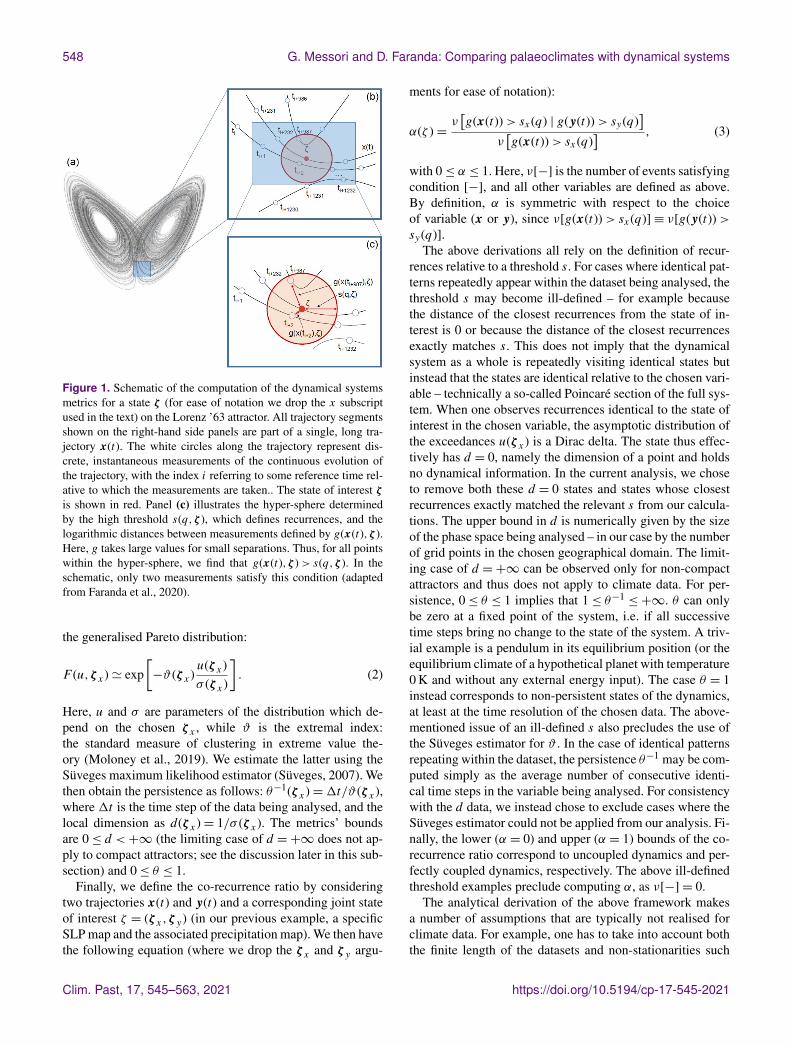
We next define a high-threshold s(q,ζ x) as the qth quan-tile of g(x(t),ζ x) (here q = 0.98) and define exceedancesu(ζ x)= g(x(t),ζ x)−s(q,ζ x)∀g(x(t),ζ x)> s(q,ζ x). Theseare effectively the previously mentioned Poincaré recur-rences for the chosen state ζ x . The interpretation of the abovequantities for the idealised case of the Lorenz ’63 attractor(Lorenz, 1963) – a simple three-dimensional dynamical sys-tem – is illustrated graphically in Fig. 1. We then leverage theFreitas–Freitas–Todd theorem (Freitas et al., 2010; Lucariniet al., 2012), which states that the cumulative probability dis-tribution F (u,ζ x) converges to the exponential member of

https://doi.org/10.5194/cp-17-545-2021 Clim. Past, 17, 545–563, 2021


Figure 1. Schematic of the computation of the dynamical systemsmetrics for a state ζ (for ease of notation we drop the x subscriptused in the text) on the Lorenz ’63 attractor. All trajectory segmentsshown on the right-hand side panels are part of a single, long tra-jectory x(t). The white circles along the trajectory represent dis-crete, instantaneous measurements of the continuous evolution ofthe trajectory, with the index i referring to some reference time rel-ative to which the measurements are taken.. The state of interest ζis shown in red. Panel (c) illustrates the hyper-sphere determinedby the high threshold s(q,ζ ), which defines recurrences, and thelogarithmic distances between measurements defined by g(x(t),ζ ).Here, g takes large values for small separations. Thus, for all pointswithin the hyper-sphere, we find that g(x(t),ζ )> s(q,ζ ). In theschematic, only two measurements satisfy this condition (adaptedfrom Faranda et al., 2020).

the generalised Pareto distribution:

F (u,ζ x)' exp[−ϑ(ζ x)

u(ζ x)σ (ζ x)

]. (2)

Here, u and σ are parameters of the distribution which de-pend on the chosen ζ x , while ϑ is the extremal index:the standard measure of clustering in extreme value the-ory (Moloney et al., 2019). We estimate the latter using theSüveges maximum likelihood estimator (Süveges, 2007). Wethen obtain the persistence as follows: θ−1(ζ x)=1t/ϑ(ζ x),where 1t is the time step of the data being analysed, and thelocal dimension as d(ζ x)= 1/σ (ζ x). The metrics’ boundsare 0≤ d <+∞ (the limiting case of d =+∞ does not ap-ply to compact attractors; see the discussion later in this sub-section) and 0≤ θ ≤ 1.

Finally, we define the co-recurrence ratio by consideringtwo trajectories x(t) and y(t) and a corresponding joint stateof interest ζ = (ζ x,ζ y) (in our previous example, a specificSLP map and the associated precipitation map). We then havethe following equation (where we drop the ζ x and ζ y argu-

ments for ease of notation):

α(ζ )=ν[g(x(t))> sx(q) | g(y(t))> sy(q)

]ν[g(x(t))> sx(q)

] , (3)

with 0≤ α ≤ 1. Here, ν[−] is the number of events satisfyingcondition [−], and all other variables are defined as above.By definition, α is symmetric with respect to the choiceof variable (x or y), since ν[g(x(t))> sx(q)] ≡ ν[g(y(t))>sy(q)].

The above derivations all rely on the definition of recur-rences relative to a threshold s. For cases where identical pat-terns repeatedly appear within the dataset being analysed, thethreshold s may become ill-defined – for example becausethe distance of the closest recurrences from the state of in-terest is 0 or because the distance of the closest recurrencesexactly matches s. This does not imply that the dynamicalsystem as a whole is repeatedly visiting identical states butinstead that the states are identical relative to the chosen vari-able – technically a so-called Poincaré section of the full sys-tem. When one observes recurrences identical to the state ofinterest in the chosen variable, the asymptotic distribution ofthe exceedances u(ζ x) is a Dirac delta. The state thus effec-tively has d = 0, namely the dimension of a point and holdsno dynamical information. In the current analysis, we choseto remove both these d = 0 states and states whose closestrecurrences exactly matched the relevant s from our calcula-tions. The upper bound in d is numerically given by the sizeof the phase space being analysed – in our case by the numberof grid points in the chosen geographical domain. The limit-ing case of d =+∞ can be observed only for non-compactattractors and thus does not apply to climate data. For per-sistence, 0≤ θ ≤ 1 implies that 1≤ θ−1

≤+∞. θ can onlybe zero at a fixed point of the system, i.e. if all successivetime steps bring no change to the state of the system. A triv-ial example is a pendulum in its equilibrium position (or theequilibrium climate of a hypothetical planet with temperature0 K and without any external energy input). The case θ = 1instead corresponds to non-persistent states of the dynamics,at least at the time resolution of the chosen data. The above-mentioned issue of an ill-defined s also precludes the use ofthe Süveges estimator for ϑ . In the case of identical patternsrepeating within the dataset, the persistence θ−1 may be com-puted simply as the average number of consecutive identi-cal time steps in the variable being analysed. For consistencywith the d data, we instead chose to exclude cases where theSüveges estimator could not be applied from our analysis. Fi-nally, the lower (α = 0) and upper (α = 1) bounds of the co-recurrence ratio correspond to uncoupled dynamics and per-fectly coupled dynamics, respectively. The above ill-definedthreshold examples preclude computing α, as ν[−] = 0.

The analytical derivation of the above framework makesa number of assumptions that are typically not realised forclimate data. For example, one has to take into account boththe finite length of the datasets and non-stationarities such



as those issuing from internal low-frequency variability orvarying external forcing. A formal justification of the appli-cability of the dynamical systems metrics to finite data is-sues from the results of Caby et al. (2020). There, the authorsshow that finite-time deviations of d and θ from the asymp-totic, unknown values contain information about the underly-ing system, since they are linked to the presence of unstableor periodic points of the dynamics. Similarly, both analyt-ical and empirical evidence from Pons et al. (2020) showsthat, although affected by the curse of dimensionality, esti-mates of d from finite time series may be used in a relativesense to characterise the dynamics of a system – i.e. by com-paring values of d to one another. The conclusions drawnfrom these more theoretical results match those issuing fromempirical tests on climate time series of finite length con-ducted by Buschow and Friederichs (2018). In practice, thetwo metrics may thus be applied to a variety of datasets issu-ing from chaotic dynamical systems, including (weakly non-stationary) climate datasets (e.g. Faranda et al., 2019c, 2020;Brunetti et al., 2019).

MATLAB code to compute d, θ−1 and α is provided at theend of this paper under “Code availability”.

3 Dynamical systems in action: an example from themid-Holocene Green Sahara

3.1 The mid-Holocene Green Sahara: background anddata

Today, the Sahara is the largest hot desert on Earth. Most ofthe precipitation in north-western Africa is associated withthe West African Monsoon (WAM), which reaches to around16–17◦ N (e.g. Sultan and Janicot, 2003) and effectively setsthe boundary between the semiarid Sahel and the Sahara.However, the region has repeatedly experienced momentoushydroclimatic shifts in the past. In particular, there have beenseveral periods when the Sahara was wetter and greener thantoday, often termed “African Humid Periods” (AHPs; seeClaussen et al., 2017 and Pausata et al., 2020, for recent re-views on the topic).

The most recent AHP peaked during the mid-Holocene(MH), approximately 9000–6000 years BP. It is thought tohave coincided with an intensification and northward shiftof the WAM, allowing the presence of vegetation, lakes andwetlands in areas that today are desert (e.g. Holmes, 2008,and references therein). Palaeo-archives suggest that duringthe MH AHP, summer precipitation reached the northernparts of the present-day desert (e.g. Sha et al., 2019) and thattropical vegetation may have extended as far as 24◦ N (Hélyet al., 2014).

Numerical climate simulations of the MH have struggledto reproduce the full extent of the monsoonal intensificationsuggested by the palaeo-archives, and commonly suffer froma dry bias (Harrison et al., 2014). Early investigations onthe topic highlighted the large sensitivity of the simulations

to land surface characteristics (e.g. Kutzbach et al., 1996;Kutzbach and Liu, 1997; Claussen and Gayler, 1997). Morerecent modelling efforts have confirmed this and have furtherhighlighted the potential role of an incorrect representation ofatmospheric aerosols in favouring the dry bias (Pausata et al.,2016; Gaetani et al., 2017; Messori et al., 2019). Such a hy-pothesis has triggered a lively discussion in the literature (cf.Thompson et al., 2019; Hopcroft and Valdes, 2019).

Here, we analyse the simulations used in Messori et al.(2019), performed with the EC-Earth Earth System Modelv3.1 (Hazeleger et al., 2010). The atmospheric model hasa T159 horizontal spectral resolution and 62 vertical levels.The ocean model has a nominal horizontal resolution of 1◦

and 46 vertical levels. In all simulations, the vegetation andaerosol concentrations are prescribed.

To illustrate the dynamical systems approach described inSect. 2, we consider three different simulations. The firstis a MH control simulation (MHCNTL), which follows thePMIP3 protocol in imposing pre-industrial vegetation and at-mospheric dust concentrations (Braconnot et al., 2011). Thesecond is a Green Sahara simulation (MHGS+PD), which im-poses shrubland over the region 11–33◦ N and 15◦W–35◦ E.The third is a Green Sahara simulation that, in addition to thevegetation, also imposes a strongly reduced atmospheric dustloading (MHGS+RD). Indeed, a greening of the Sahara wouldintuitively correspond to decreased dust emissions and henceto a lower atmospheric loading, as also supported by palaeo-archives (Demenocal et al., 2000; McGee et al., 2013) andmodelling studies (Egerer et al., 2016).

We analyse 30 years of daily data of sea level pressure(SLP), 500 hPa geopotential height (Z500) and precipita-tion frequency (prp) for each simulation. Precipitation fre-quency is constructed by assigning a value of 1 to grid pointsand time steps with non-zero precipitation and a value of0 otherwise. This is preferable to using raw precipitationdata for estimating the dynamical systems metrics (and d inparticular), as discussed further in Langousis et al. (2009)and Faranda et al. (2017a). As a technical consideration,we underline that the binary discretisation does not affectthe spatio-temporal fractal nature of the precipitation field(Lovejoy and Schertzer, 1985; Brunsell, 2010). Nonetheless,it does make the distance dist a fundamentally different kindof random variable than for SLP and Z500, because its den-sity consists of a finite number of point masses. The membersof the extreme value distribution family, on the other hand,are continuous functions. Although there is no complete the-oretical framework for the application of extreme value the-ory to recurrences of discrete fields, the analysis by Hitz(2016) supports the physical relevance of the results. Anotherissue with the precipitation data is that there can be repeatedidentical precipitation patterns (e.g. when there is no pre-cipitation over the chosen domain). The implications of thisfor estimating the dynamical systems metrics are discussedin Sect. 2.2. We define the pre-monsoon season as March,April and May (MAM) and the monsoon season as June,



July, August and September (JJAS). These definitions arebased on the present-day WAM climatology. We use them inour analysis as reference periods when comparing the threenumerical simulations described above. We quantify statis-tically significant differences when comparing median val-ues of datasets using the Wilcoxon rank sum test (Wilcoxon,1945) at the 1 % significance level. For the geographical pre-cipitation anomalies, one-sided 5 % significance bounds aredetermined using bootstrap resampling with 1000 iterations.

3.2 A dynamical systems view of the mid-HoloceneGreen Sahara

The main interest in analysing the above simulations lies inunderstanding whether and why they reproduce different hy-droclimates over the Sahelian–Saharan region. Our aim inthis section is not to systematically investigate these two as-pects but instead to illustrate how the dynamical systemsframework proposed here can be used to characterise the in-dividual simulations and provide a concise overview of thedifferences between them. We argue that such an approachcan provide a valuable complement to conventional analyses,and we relate our results to those obtained in earlier studies(e.g. Pausata et al., 2016; Gaetani et al., 2017; Messori et al.,2019).

A simple composite of JJAS average precipitation immedi-ately highlights large differences in the precipitation regimes,with the MHGS+PD simulation showing a large northwardshift and intensification of the monsoonal precipitation com-pared to MHCNTL (Fig. 2a, b) and the MHGS+RD simulationshowing an additional, albeit smaller, precipitation increase(Fig. 2c, d). However, this time mean picture hides a num-ber of complex dynamical changes in the WAM, which weinvestigate using our dynamical systems framework. We fo-cus on the northern WAM region (12.5–30◦ N, 10◦W–20◦ E,black box in Fig. 2a). This domain is chosen to reflect the re-gion of seasonal monsoon rainfall that we expect to be mostaffected by the changes in land surface and atmospheric dustloading. Results for a more geographically extended domainare shown in Appendix A.

We begin by studying the seasonality of d and θ−1 for pre-cipitation data. In the MHCNTL (Fig. 3a, blue curve), the localdimension displays a marked interannual variability for anygiven calendar day, which we ascribe to the large variabil-ity in the monsoonal precipitation reproduced by the model(Fig. 3c, blue curve). The fact that the local dimension’s vari-ability peaks in the pre-monsoon season, while that of pre-cipitation itself peaks during the monsoon season, is likelyrelated to the use of precipitation frequency, which makesthe local dimension more sensitive to changes in the timingof rain onset than to rain amount. This provides an insightinto the potentially large onset variations within the samemodel simulation – an aspect which does not emerge fromthe variability of the zonally averaged precipitation climatol-ogy. The seasonal cycle of the local dimension displays two

peaks, roughly matching the onset and withdrawal phases ofthe monsoon, somewhat lower values during the height of thesummertime monsoon, and the lowest values during the dryseason. Previous studies have noted how transition periodscan display an increase in the local dimension of atmosphericfields because the atmosphere explores configurations be-longing to more than one season (Faranda et al., 2017b). Inmore technical terms, this would reflect a saddle-like pointof the atmospheric dynamics. We therefore interpret the twolocal maxima in d as reflecting the northward shift and re-treat of the monsoonal rainfall. The local dimension in theMHGS+PD and MHGS+RD simulations (red and orange curves,respectively) presents a similar seasonal cycle, yet with thefirst local maximum shifted to earlier in the year, the secondlocal maximum shifted to later in the year (Fig. 3b) and lowervalues throughout the monsoon season. Indeed, the medi-ans of d during the monsoon season in the MHGS+PD andMHGS+RD simulations are significantly different to that in theMHCNTL simulation. The shift of the local maxima points toa lengthening of the monsoon season, with an earlier rain-fall onset and a later withdrawal. The timing of the first lo-cal maximum in d indeed coincides with a rapid increasein the zonally averaged precipitation at the southern edgeof the domain in the MHGS+PD and MHGS+RD simulations(Fig. 3c). Such a lengthening of the monsoonal period un-der a greening of the Sahara was previously noted in Pausataet al. (2016) by adopting a monsoon duration algorithm.The seasonal cycle of θ in MHCNTL (Fig. 3b, blue curve)displays a very different pattern. Low values (high persis-tence) occur during the monsoon season, while higher values(lower persistence) occur during the dry season, albeit witha very large spread. This may reflect sporadic rainfall eventsat the edges of the domain outside of the monsoon season,with more persistent precipitation patterns during the mon-soon season. The MHGS+PD and MHGS+RD simulations (redand orange curves, respectively) display a similar seasonal-ity, albeit with a longer high-persistence monsoonal period,higher-persistence values during the latter period, and a moremarked difference in values between the monsoonal and dryphases. This chiefly results from lower θ values during themonsoonal period, likely reflecting a more geographicallyextensive and persistent precipitation regime. The medianθ values during the monsoon period in the MHGS+PD andMHGS+RD simulations are significantly different from thatof the MHCNTL simulation. One may hypothesise that theincreased persistence underlies a decrease in importance oftransient, mesoscale convective systems for driving the mon-soonal precipitation, in favour of a regional re-organisation ofprecipitation into larger-scale persistent features. This wouldalso explain the decrease in d during the monsoon seasonin the MHGS+PD and MHGS+RD simulations relative to theMHCNTL case. Gaetani et al. (2017) investigated the spectralproperties and mesoscale motions of the monsoonal circula-tion and concluded that the greening of the Sahara and dustreduction suppress African easterly waves and their role in



Figure 2. JJAS precipitation (mm d−1) for the (a) MHCNTL, (b) MHGS+PD and (c) MHGS+RD simulations. (d) Precipitation differencebetween the MHGS+RD and MHGS+PD simulations. The black box in panel (a) marks the domain used to perform the dynamical systemsanalysis (12.5–30◦ N, 10◦W–20◦ E).

Figure 3. Seasonal cycle of median (a) d, (b) θ and (c) zonally averaged daily precipitation (mm d−1) at 12.5◦ N for the MHCNTL (blue),MHGS+PD (red) and MHGS+RD (orange) simulations. The blue shading marks ±1 SD from the MHCNTL. The vertical dashed lines markthe pre-monsoon (MAM) and monsoon (JJAS) seasons. The data are smoothed with a 10 d moving average.



triggering precipitation. This supports the hypothesis we for-mulated here on the basis of the 1-D metric θ . The abovequalitative considerations are mostly insensitive to the exactchoice of geographical domain (cf. Figs. 3 and A2).

The seasonal variations in d and θ can also be related tovariations in the dynamical indicators on shorter timescales.The fact that a rapid increase in d and a corresponding de-crease in θ coincide with the northward progression of mon-soonal rainfall indeed suggests that concurring high d valuesand low θ values on daily timescales may correspond to spe-cific spatial precipitation patterns. To verify this, we computecomposite rainfall anomalies during JJAS on days with con-current d anomalies above the 70th percentile and θ anoma-lies below the 30th percentile of the respective JJAS distri-butions (Fig. 4). These relatively broad ranges are needed toensure a good sample of dates, since here we are imposinga condition on each of the two metrics simultaneously. Theanomalies are defined as deviations from a daily seasonal cy-cle. For example, the climatological value of a given vari-able in a given simulation for the 22 July, is the mean of thatvariable across all 22 July days in the simulation. Applyinga smoothing to the climatology leads to very minor quantita-tive changes in our results (not shown). In MHCNTL (Fig. 4a),the anomalies are limited to the southern part of the domain,as the bulk of the Sahara receives little or no precipitationeven at the peak of the monsoon (see Fig. 2a). The spatialpattern of the anomalies is wave-like, albeit with limited sta-tistical significance, pointing to the fact that the dynamicalsystems metrics may reflect modulations in African easterlywave activity (see, e.g. Fig. 8 in Gaetani et al., 2017, and thediscussion above). The MHGS+PD and MHGS+RD simulationsinstead display clear and statistically significant anomalydipoles, oriented in a predominantly meridional direction butwith some zonal asymmetry. These correspond to a north-ward shift of the monsoonal precipitation relative to the cli-matology (Fig. 4b and c, respectively). The dipoles span thewhole domain and display the largest anomaly values in theMHGS+RD simulation. This is indeed the simulation showingthe largest total rainfall, as well as the strongest northwardshift of the monsoonal precipitation range (Fig. 2d). Verysimilar results are obtained if the same calculation is repeatedover a larger domain (Fig. A3).

We next try to understand the physical processes underly-ing the differences in precipitation in the three simulations,by computing the co-recurrence ratio α between SLP andprp (Fig. 5a). In MHCNTL (blue line), as the monsoonal pre-cipitation progresses northwards the coupling between thetwo variables increases, peaking in the middle of the mon-soon season and waning thereafter. The dry season is charac-terised by overall low coupling values. In the MHGS+PD andMHGS+RD simulations (red and orange curves, respectively),α displays two local minima in the pre-monsoon season andin autumn. During the northward progression of precipita-tion and the peak monsoonal phase, the values are mostlyhigher than for the MHCNTL simulation. Indeed, the median

α values during the monsoon season of the MHGS+PD andMHGS+RD simulations are significantly different to those ofthe MHCNTL simulation. Both simulations also show higherα values than MHCNTL during the dry season, although thesevalues are generally lower than in the monsoonal period.Similar results are found when extending the geographicaldomain (cf. Figs. 5 and A4), albeit with slightly higher cou-pling values for the extended domain during the dry season.These are likely associated to the presence of more abun-dant wintertime precipitation at the latter domain’s southernboundary (Fig. A5). The stronger coupling in the MHGS+PDand MHGS+RD simulations compared to the MHCNTL duringthe pre-monsoon and monsoon seasons, points to the role ofcirculation anomalies – reflected in the SLP field – in favour-ing the northwards extension of the monsoonal precipitation.This was indeed noted in Pausata et al. (2016) by analysingchanges in lower-level atmospheric thickness related to theSaharan heat low (see also Lavaysse et al., 2009). The higherα values during wintertime in the MHGS+PD and MHGS+RDsimulations may once again be related to the presence of lim-ited amounts of winter precipitation in the domain while pre-cipitation is almost entirely absent in the MHCNTL simulation(Fig. A5). A similar picture is found for the co-recurrenceratio between Z500 and prp (Fig. 5b and Fig. A4b), high-lighting the robust nature of the increased coupling betweenprecipitation and large-scale atmospheric circulation featuresin the MHGS+PD and MHGS+RD simulations.

As for d and θ above, one may relate the seasonal vari-ations in α to the daily anomalies associated with large orsmall values of the metric. We specifically consider precip-itation, SLP and Z500 anomalies (computed as in Fig. 4)on JJAS days when α exceeds the 95th percentile of itsanomaly distribution. These “strong coupling” days may beconceptualised as days on which recurrent spatial large-scalecirculation anomalies favour recurrent spatial precipitationanomalies. In MHCNTL, this takes the form of significantlyincreased precipitation across the southern portion of the do-main, favoured by negative SLP anomalies to the north of thestrongest precipitation anomalies (Fig. 6a) and positive Z500anomalies to the north of the negative SLP core (cf. Fig. 6aand Fig. 7a). These are likely the footprint of a strengthenedheat low (see, e.g. Fig. 2b in Lavaysse et al., 2009), whichfavours a northward progression of the monsoonal precipita-tion. As noted above, the signal being limited to the southernpart of the domain is due to the MHCNTL simulation display-ing little or no precipitation in the more northerly parts of thedomain. The MHGS+PD simulation shows a statistically sig-nificant, predominantly zonal dipole, with positive precipita-tion anomalies in the eastern part of the domain and negativeanomalies further west (Figs. 6b and Fig. 7b). On strong cou-pling days, the large-scale circulation therefore favours aneastward extension of precipitation into a region that, evenunder a vegetated Sahara, receives little precipitation (seeFig. 2b). The SLP composite anomalies broadly match theones of the MHCNTL simulation, while the Z500 anomalies



Figure 4. JJAS precipitation anomalies (mm d−1) on days with high d and low θ (see text) for the (a) MHCNTL, (b) MHGS+PD and(c) MHGS+RD simulations. The anomalies are only shown over the domain used to perform the dynamical systems analysis (see the blackbox in Fig. 2a). Bold lines mark significance bounds (see text).

Figure 5. Seasonal cycle of median (a) αSLP,PRP and (b) αZ500,PRP for the MHCNTL (blue), MHGS+PD (red) and MHGS+RD (orange)simulations. The blue shading marks ±1 SD from the MHCNTL. The vertical dashed lines mark the pre-monsoon (MAM) and monsoon(JJAS) seasons. The data are smoothed with a 10 d moving average.

are much larger in magnitude. The MHGS+RD simulation re-sembles the MHGS+PD simulation for the Z500 case, albeitwith weaker geopotential height anomalies (Fig. 7c). An in-verted precipitation dipole, with a significantly drier easternpart of the domain and a significantly wetter northwesternpart, is instead seen for the SLP composite (Fig. 6c). Com-

parable results are found when extending the geographicaldomain, with some differences that we partly ascribe to theeffect of α capturing some tropical precipitation patterns atthe southern edge of the domain (cf. Fig. 6 and Fig. 7 withFig. A6 and Fig. A7). A hypothesis to explain the differencesbetween the MHGS+PD and MHGS+RD simulations is that in



Figure 6. JJAS precipitation (colours, mm d−1) and SLP (contours, hPa) anomalies on days with high α (see text) for the (a) MHCNTL,(b) MHGS+PD and (c) MHGS+RD simulations. The contour lines have an interval of 0.25 hPa and span the following ranges: (a) −0.25 to−1.5 hPa, (b) −0.25 to −1.25 hPa and (c) +0.5 to −0.75 hPa. Continuous contours show zero and positive anomalies, and dashed contoursshow negative anomalies. The anomalies are only shown over the domain used to perform the dynamical systems analysis (see the black boxin Fig. 2a). Bold lines mark significance bounds for precipitation (see text).

Figure 7. JJAS precipitation (colours, mm d−1) and Z500 (contours, m) anomalies on days with high α (see text) for the (a) MHCNTL,(b) MHGS+PD and (c) MHGS+RD simulations. The contour lines have an interval of 20 m and span the following ranges: (a) +40 to −40 m,(b) +60 to −100 m and (c) +60 to −20 m. Continuous contours show zero and positive anomalies, and dashed contours show negativeanomalies. The anomalies are only shown over the domain used to perform the dynamical systems analysis (see the black box in Fig. 2a).Bold lines mark significance bounds for precipitation (see text).



the latter enhanced deep convection triggered by large up-ward heat fluxes over the Sahara plays a larger role in shap-ing precipitation (Gaetani et al., 2017). This is in agreementwith the increased amount of locally recycled moisture overthe Sahara driven by dust reduction under a vegetated Sahara,as noted by Messori et al. (2019).

The above results illustrate some of the strengths and lim-itations of the analysis framework we propose in this work,which we discuss further in Sect. 4 below. If applied in thecontext of a full-length research paper, some of the hypothe-ses expounded here could be verified through additional anal-yses. These could include, for example, the use of lower-level atmospheric thickness or other tailored indicators ofheat low activity, of atmospheric radiative and heat fluxes,and of moist static energy as an indicator of convection.

4 An appraisal of the dynamical systems frameworkin a palaeoclimate context

Palaeoclimate simulations of the same period and region mayyield very different results, the understanding of which re-quires analysis tools that may efficiently distil the discrep-ancies and point to possible underlying drivers. In this tech-nical note, we have outlined an analysis framework whichcan efficiently compare the salient dynamical features of dif-ferent simulated palaeoclimates. The framework is groundedin dynamical systems theory and rests on computing threemetrics: the local dimension d, the persistence θ−1 and theco-recurrence ratio α. The first two metrics inform on theevolution of a system about a given state of interest – for ex-ample how the atmosphere evolves to or from a given large-scale configuration. The third metric describes the couplingbetween different variables.

From a theoretical standpoint, the dynamical systemsframework presents a number of advantages over other sta-tistical approaches for the analysis of large amounts of cli-mate data such as clustering, principal component analy-sis or canonical correlation analysis. The first two are oftenused to define climate variability modes or weather regimes.The d and θ metrics reflect the information captured bypartitioning the atmospheric variability into specific regimes(e.g. Faranda et al., 2017a; Hochman et al., 2019), yet theyalso provide additional information on how the atmosphereevolves within and between the regimes. Canonical correla-tion analysis (CCA), which identifies maximum-correlationlinear combinations of two variables, provides informationwhich largely overlaps that given by α (De Luca et al.,2020b). However, the latter may be flexibly applied to multi-variate cases beyond two variables, without the need for spe-cific adaptations (such as partial CCA). Further, while sta-tistical techniques can provide valuable information on theevolution of the climate system, the dynamical indicators wepropose here are rooted in the system’s underlying dynamics.In other words, their values are projections of mathematical

properties of the underlying equations of the system, evenwhen these are unknown. For example, a low local dimensionnot only points to a specific metastable state of the dynamics– as is the case for a conventionally defined weather regime– but also shows that this state is in a predictable region ofthe attractor. Moreover, the computation of the dynamicalsystems metrics requires essentially a single free parameterto be fixed, namely the threshold to define recurrences, andone may easily test the stability of the estimates with respectto small perturbations to this threshold. Furthermore, stateswith θ→ 0 indicate quasi-singularities – technically unsta-ble fixed points – of the system. Quasi-singular states por-tend tipping points or tipping elements of the climate systemthat have not yet been crossed (e.g. Lenton et al., 2008) andcan thus be of interest for a range of palaeoclimate appli-cations. Indeed, analysis of data issuing from both concep-tual (Faranda et al., 2019c) and reduced-complexity (Mes-sori et al., 2021) models of specific features of atmosphericdynamics have highlighted that changes in d and θ values re-flect transitions between different basins of attraction of thesystem. Finally, the metrics provide one value for every timestep in the analysed data, and may be conveniently used to in-vestigate seasonality, oscillatory behaviours, high-frequencyvariability and more. This is especially valuable for the co-recurrence ratio, as a number of other measures of couplingor correlation between two variables only provide a singlevalue for the whole time period being considered.

Because of these characteristics, the dynamical systemsmetrics can be particularly helpful when processing largedatasets (see, e.g. Rodrigues et al., 2018; Faranda et al.,2019a). To illustrate their practical applicability in palaeocli-mate studies, we have analysed three numerical simulationsof the mid-Holocene climate over North Africa: a controlsimulation with pre-industrial vegetation and atmosphericdust loading, a Green Sahara simulation with shrubland im-posed over a broad swath of what is today the Sahara desert,and a second Green Sahara simulation that additionally fea-tures heavily reduced atmospheric dust loading. Our aim isto show that the different hydroclimates in these simulationscorrespond to different dynamical properties of the modelledclimate systems, which are captured by the three dynamicalsystems metrics. The seasonal cycles of d and θ−1 reflect fea-tures of the duration, interannual variability and geograph-ical extent of the monsoon, which do not always emergeclearly from the precipitation’s seasonal cycle. The metricsfurther capture the differences between the simulations andmay be leveraged to formulate hypotheses on their physicaldrivers, such as modulations in atmospheric wave activity.The co-recurrence ratio α, which provides a temporally re-solved measure of coupling between different variables, en-riches the picture by enabling the contextualisation of precip-itation changes relative to large-scale atmospheric circulationanomalies.

As a caveat, we note that our approach is more successfulin providing insights into the changes between the control



and each of the Green Sahara simulations than between thelatter two simulations. Previous analyses of these same sim-ulations and studies from other authors (e.g. Pausata et al.,2016; Thompson et al., 2019) suggest that, compared tothe effect of Saharan Greening, the dust reduction under aGreen Sahara scenario only has limited impacts on the at-mospheric circulation. This points to our framework beingbest suited for diagnosing shifts in palaeoclimate dynamics,as opposed to smaller climatological changes not associatedwith changes in the underlying driving processes.

Additionally, obtaining good estimates of d, θ−1 and αrequires relatively long time series, limiting their applica-bility to palaeo-archives. At the same time, empirical evi-dence shows that daily time series of a few decades – as of-ten obtained from numerical simulations – are typically suf-ficient for many climate applications. Indeed, previous stud-ies have outlined that the estimates of the metrics for atmo-spheric observables convergence relatively fast (e.g. Farandaet al., 2017a; Buschow and Friederichs, 2018). There are nofixed rules for determining the minimum required amount ofdata, but current best practice is to have several good recur-rences of the patterns of interest in the data. While no formaldefinition of what constitutes a “good recurrence” is forth-coming, a simple test that may be applied is to reduce thelength of the datasets being used and repeat the metrics’ esti-mates to check their stability (e.g. Buschow and Friederichs,2018). Non-stationary data, such as may be found in tran-sient palaeoclimate simulations, also require some care inverifying that recurrences can be identified (see also Sect. 2).Our methodology is able to detect weak non-stationarities inthe climate system, as for example is the case for the ongo-ing climate change (e.g. Faranda et al., 2019a). However, anabrupt regime shift poses a different challenge, and it is anopen question as to what the limit of validity of our metricsfor non-stationary systems is. A further difficulty that maybe encountered in applying the dynamical systems frame-work pertains to its interpretation. While the three metricslend themselves to making relatively intuitive heuristic infer-ences, they may sometimes provide counterintuitive results,such as Figs. 6c and 7c here, and there is no universally validapproach to overcome these interpretative difficulties. Fur-thermore, expounding formal arguments to support the re-sults obtained requires a detailed knowledge of the underly-ing theoretical bases, which may initially be daunting.

In this technical note, we aimed to give a taste of the dy-namical systems framework’s possible application to palaeo-climate simulations, as opposed to presenting a systematicanalysis. We specifically wished to highlight its potential forcomparing different palaeoclimates while also providing anappraisal of its limitations. To do so, we focussed on threeexisting simulations and on a small number of atmosphericvariables. However, the approach is relevant to a very broadrange of palaeoclimate applications and is thus not limitedto the comparison of different climates or to the atmosphere.In particular, the co-recurrence coefficient could be used tostudy interactions between the different components of theclimate system varying on different timescales, such as thehydrosphere and the atmosphere or the hydrosphere and thecryosphere (e.g. by comparing the response of different nu-merical models to the same forcing). As mentioned above, θmay also have a direct application in the detection of tippingpoints or states. From a technical perspective, we envisagethat the most effective application of the framework wouldbe for the analysis of very large datasets, such as those is-suing from the PMIP initiative or from downscaling effortson very long transient simulations (e.g. Lorenz et al., 2016).At the same time, we stress that we do not view the frame-work as a wholesale substitute for conventional analyses ofpalaeoclimate dynamics. Rather, it is intended as a comple-ment that may help to strengthen mechanistic interpretationsand rapidly identify features deserving further investigation.



Appendix A: Additional figures

In this appendix, we provide a schematic of the raindrop anal-ogy for the dynamical systems metrics and figures illustratingthe sensitivity of our results to the choice of geographical do-main and season. The figures are discussed in the main text.

Figure A1. The raindrop analogy for the dynamical systems metrics. (a) Depending on the topography, raindrops falling on a small patchof ground on the side of a valley may follow similar paths (low local dimension) or different paths (high local dimension). (b) If the patchof ground is on a steep incline, the raindrops will leave it very rapidly (low persistence); if the incline is shallow, the raindrops will takelonger to leave the patch (high persistence). (c, d) Vegetation will affect the raindrop paths, and at the same time the paths of the raindropswill affect the growth of the vegetation. Whenever the raindrops collectively follow similar paths, this will correspond to a recurring patternof vegetation growth and vice versa (high co-recurrence ratio). Part of the figure has been excerpted from Marshak (2019), with permissionof the publisher, W. W. Norton & Company, Inc. All rights reserved (Copyright © 2019, 2015, 2012, 2008, 2005, 2001 by W. W. Norton &Company, Inc.).

Figure A2. The same as Fig. 3a and b but using the domain 10–30◦ N, 15◦W–20◦ E.



Figure A3. The same as Fig. 4 but using the domain 10–30◦ N, 15◦W–20◦ E.

Figure A4. The same as Fig. 5 but using the domain 10–30◦ N, 15◦W–20◦ E.



Figure A5. The same as Fig. 2 but for the October–February period.

Figure A6. The same as Fig. 6 but using the domain 10–30◦ N, 15◦W–20◦ E. The contour lines have an interval of 0.25 hPa and span thefollowing ranges: (a) −0.25 to −1.25 hPa, (b) 0 to −1.5 hPa, and (c) +0.25 to −0.75 hPa.



Figure A7. The same as Fig. 7 but using the domain 10–30◦ N, 15◦W–20◦ E. The contour lines have an interval of 20 m and span thefollowing ranges: (a) +40 to −20 m, (b) +60 to −80 m, and (c) +60 to −20 m.



Code availability. The code to compute the three dynamical sys-tems indicators used in this study is made freely available throughthe cloud storage of the Centre National de la Recherche Scien-tifique (CNRS) under a CC BY-NC 3.0 license: https://mycore.core-cloud.net/index.php/s/pLJw5XSYhe2ZmnZ (Faranda, 2021).

Data availability. The EC-Earth model data are stored as global3-D or 4-D NetCDF files and exceed the size limitations of most on-line repositories. The files needed to reproduce the results presentedin this study may be obtained upon request to the corresponding au-thor.

Author contributions. GM conceived the study and performedthe analysis. DF provided the publicly available code. Both authorscontributed to drafting the manuscript.

Competing interests. The authors declare that they have no con-flict of interest.

Acknowledgements. The authors thank Francesco Pausata,Qiong Zhang and Marco Gaetani for making the palaeoclimate sim-ulations available. We also thank the two anonymous reviewers forthe detailed and pertinent comments they provided.

Financial support. Gabriele Messori has been partly sup-ported by the Swedish Research Council Vetenskapsrådet (grantno. 2016-03724) and the Swedish Research Council for SustainableDevelopment FORMAS (grant no. 2018-00968). Davide Farandawas supported by a CNRS/INSU LEFE/MANU grant (DINCLICproject) and by an ANR-TERC grant (BOREAS project).

The article processing charges for this open-accesspublication were covered by Stockholm University.

Review statement. This paper was edited by Martin Claussenand reviewed by Christian Franzke and one anonymous referee.

References

Barron, E. J., Sloan II, J., and Harrison, C.: Potential significance ofland–sea distribution and surface albedo variations as a climaticforcing factor; 180 my to the present, Palaeogeogr. Palaeoclim.Palaeoecol., 30, 17–40, 1980.

Bartlein, P. J., Harrison, S., Brewer, S., Connor, S., Davis, B.,Gajewski, K., Guiot, J., Harrison-Prentice, T., Henderson, A.,Peyron, O., Prentice, C., Scholze, M., Seppa, H., Shuman, B.,Sugita, S., Thompson, R. S., Viau, A. E., Williams, J., and Wu,H.: Pollen-based continental climate reconstructions at 6 and21 ka: a global synthesis, Clim. Dyn., 37, 775–802, 2011.

Braconnot, P., Harrison, S., Otto-Bliesner, B., Abe-Ouchi, A., Jung-claus, J., and Peterschmitt, J.: The paleoclimate modeling Inter-

comparison project contribution to CMIP5, CLIVAR Exchanges,56, 15–19, 2011.

Brunetti, M., Kasparian, J., and Vérard, C.: Co-existing climate at-tractors in a coupled aquaplanet, Clim. Dyn., 53, 6293–6308,2019.

Brunsell, N.: A multiscale information theory approach to assessspatial–temporal variability of daily precipitation, J. Hydrol.,385, 165–172, 2010.

Buschow, S. and Friederichs, P.: Local dimension and recur-rent circulation patterns in long-term climate simulations,Chaos: An Interdisciplinary J. Nonlinear Sci., 28, 083124,https://doi.org/10.1063/1.5031094, 2018.

Caby, T., Faranda, D., Vaienti, S., and Yiou, P.: Extreme valuedistributions of observation recurrences, Nonlinearity, 34, 118,https://doi.org/10.1088/1361-6544/abaff1, 2020.

Claussen, M. and Gayler, V.: The greening of the Sahara duringthe mid-Holocene: results of an interactive atmosphere-biomemodel, Global Ecol. Biogeogr., 6, 369–377, 1997.

Claussen, M., Dallmeyer, A., and Bader, J.: Theory and modelingof the African humid period and the green Sahara, in: OxfordResearch Encyclopedia of Climate Science, Oxford UniversityPress, Oxford, UK, 2017.

De Luca, P., Messori, G., Faranda, D., Ward, P. J., andCoumou, D.: Compound warm–dry and cold–wet eventsover the Mediterranean, Earth Syst. Dynam., 11, 793–805,https://doi.org/10.5194/esd-11-793-2020, 2020a.

De Luca, P., Messori, G., Pons, F. M., and Faranda, D.: Dynamicalsystems theory sheds new light on compound climate extremesin Europe and Eastern North America, Q. J. Roy. Meteor. Soc.,146, 1636–1650, https://doi.org/10.1002/qj.3757, 2020b.

Demenocal, P., Ortiz, J., Guilderson, T., Adkins, J., Sarnthein, M.,Baker, L., and Yarusinsky, M.: Abrupt onset and termination ofthe African Humid Period:: rapid climate responses to gradualinsolation forcing, Quaternary Sci. Rev., 19, 347–361, 2000.

Donn, W. L. and Shaw, D. M.: Model of climate evolution basedon continental drift and polar wandering, Geol. Soc. Am. B., 88,390–396, 1977.

Egerer, S., Claussen, M., Reick, C., and Stanelle, T.: The link be-tween marine sediment records and changes in Holocene Saharanlandscape: simulating the dust cycle, Clim. Past, 12, 1009–1027,https://doi.org/10.5194/cp-12-1009-2016, 2016.

Faranda, D.: Dyn_Sys_Analysis_Matlab_Package, avail-able at: https://mycore.core-cloud.net/index.php/s/pLJw5XSYhe2ZmnZ, last access: 25 February 2021.

Faranda, D., Messori, G., Alvarez-Castro, M. C., and Yiou, P.: Dy-namical properties and extremes of Northern Hemisphere climatefields over the past 60 years, Nonlin. Processes Geophys., 24,713–725, https://doi.org/10.5194/npg-24-713-2017, 2017a.

Faranda, D., Messori, G., and Yiou, P.: Dynamical proxies of NorthAtlantic predictability and extremes, Sci. Rep.-UK, 7, 41278,https://doi.org/10.1038/srep41278, 2017b.

Faranda, D., Alvarez-Castro, M. C., Messori, G., Rodrigues, D., andYiou, P.: The hammam effect or how a warm ocean enhanceslarge scale atmospheric predictability, Nat. Commun., 10, 1–7,2019a.

Faranda, D., Messori, G., and Vannitsem, S.: Attractor dimensionof time-averaged climate observables: insights from a low-orderocean-atmosphere model, Tellus A, 71, 1–11, 2019b.


https://mycore.core-cloud.net/index.php/s/pLJw5XSYhe2ZmnZ


https://doi.org/10.1063/1.5031094

https://doi.org/10.1088/1361-6544/abaff1

https://doi.org/10.5194/esd-11-793-2020

https://doi.org/10.1002/qj.3757

https://doi.org/10.5194/cp-12-1009-2016



https://doi.org/10.5194/npg-24-713-2017

https://doi.org/10.1038/srep41278


Faranda, D., Sato, Y., Messori, G., Moloney, N. R., and Yiou, P.:Minimal dynamical systems model of the Northern Hemispherejet stream via embedding of climate data, Earth Syst. Dynam.,10, 555–567, https://doi.org/10.5194/esd-10-555-2019, 2019c.

Faranda, D., Messori, G., and Yiou, P.: Diagnosing concurrentdrivers of weather extremes: application to warm and cold daysin North America, Clim. Dyn., 54, 2187–2201, 2020.

Freitas, A. C. M., Freitas, J. M., and Todd, M.: Hitting time statisticsand extreme value theory, Probab. Theory Rel., 147, 675–710,2010.

Gaetani, M., Messori, G., Zhang, Q., Flamant, C., and Pausata, F. S.:Understanding the mechanisms behind the northward extensionof the West African Monsoon during the Mid-Holocene, J. Cli-mate, 30, 7621–7642, 2017.

Gates, W. L.: The numerical simulation of ice-age climate with aglobal general circulation model, J. Atmos. Sci., 33, 1844–1873,1976.

Gualandi, A., Avouac, J.-P., Michel, S., and Faranda, D.: The pre-dictable chaos of slow earthquakes, Sci. Adv., 6, eaaz5548,https://doi.org/10.1126/sciadv.aaz5548, 2020.

Harrison, S., Bartlein, P., Brewer, S., Prentice, I., Boyd, M., Hessler,I., Holmgren, K., Izumi, K., and Willis, K.: Climate modelbenchmarking with glacial and mid-Holocene climates, Clim.Dyn., 43, 671–688, 2014.

Haywood, A. M., Hill, D. J., Dolan, A. M., Otto-Bliesner, B. L.,Bragg, F., Chan, W.-L., Chandler, M. A., Contoux, C., Dowsett,H. J., Jost, A., Kamae, Y., Lohmann, G., Lunt, D. J., Abe-Ouchi,A., Pickering, S. J., Ramstein, G., Rosenbloom, N. A., Salz-mann, U., Sohl, L., Stepanek, C., Ueda, H., Yan, Q., and Zhang,Z.: Large-scale features of Pliocene climate: results from thePliocene Model Intercomparison Project, Clim. Past, 9, 191–209,https://doi.org/10.5194/cp-9-191-2013, 2013.

Hazeleger, W., Severijns, C., Semmler, T., Stefanescu, S., Yang, S.,Wang, X., Wyser, K., Dutra, E., Baldasano, J. M., Bintanja, R.,Bougeault, P., Caballero, R., Ekman, A. M. L., Christensen, J. H.,van den Hurk, B., Jimenez, P., Jones, C., Kållberg, P., Koenigk,T., McGrath, R., Miranda, P., van Noije, T., Palmer, T., Parodi,J. A., Schmith, T., Selten, F., Storelvmo, T., Sterl, A., Tapamo,H., Vancoppenolle, M., Viterbo, P., and Willén, U.: EC-Earth:a seamless earth-system prediction approach in action, B. Am.Meteor. Soc., 91, 1357–1364, 2010.

Hély, C., Lézine, A.-M., and contributors, A.: Holocene changes inAfrican vegetation: tradeoff between climate and water availabil-ity, Clim. Past, 10, 681–686, https://doi.org/10.5194/cp-10-681-2014, 2014.

Hitz, A.: Modelling of extremes, PhD thesis, University of Oxford,Oxford, UK, 2016.

Hochman, A., Alpert, P., Harpaz, T., Saaroni, H., and Messori, G.: Anew dynamical systems perspective on atmospheric predictabil-ity: Eastern Mediterranean weather regimes as a case study,Sci. Adv., 5, eaau0936, https://doi.org/10.1126/sciadv.aau0936,2019.

Hochman, A., Alpert, P., Kunin, P., Rostkier-Edelstein, D., Harpaz,T., Saaroni, H., and Messori, G.: The dynamics of cyclones in thetwentyfirst century: the Eastern Mediterranean as an example,Clim. Dyn., 54, 561–574, 2020a.

Hochman, A., Scher, S., Quinting, J., Pinto, J. G., andMessori, G.: Dynamics and predictability of cold spells

over the Eastern Mediterranean, Clim. Dyn., 1–18,https://doi.org/10.1007/s00382-020-05465-2, 2020b.

Holmes, J. A.: How the Sahara became dry, Science, 320, 752–753,2008.

Hopcroft, P. O. and Valdes, P. J.: On the Role of Dust-Climate Feed-backs During the Mid-Holocene, Geophys. Res. Lett., 46, 1612–1621, 2019.

Kageyama, M., Braconnot, P., Harrison, S. P., Haywood, A. M.,Jungclaus, J. H., Otto-Bliesner, B. L., Peterschmitt, J.-Y., Abe-Ouchi, A., Albani, S., Bartlein, P. J., Brierley, C., Crucifix,M., Dolan, A., Fernandez-Donado, L., Fischer, H., Hopcroft,P. O., Ivanovic, R. F., Lambert, F., Lunt, D. J., Mahowald, N.M., Peltier, W. R., Phipps, S. J., Roche, D. M., Schmidt, G.A., Tarasov, L., Valdes, P. J., Zhang, Q., and Zhou, T.: ThePMIP4 contribution to CMIP6 – Part 1: Overview and over-arching analysis plan, Geosci. Model Dev., 11, 1033–1057,https://doi.org/10.5194/gmd-11-1033-2018, 2018.

Kutzbach, J. E. and Liu, Z.: Response of the African monsoon toorbital forcing and ocean feedbacks in the middle Holocene, Sci-ence, 278, 440–443, 1997.

Kutzbach, J., Bonan, G., Foley, J., and Harrison, S.: Vegetation andsoil feedbacks on the response of the African monsoon to orbitalforcing in the early to middle Holocene, Nature, 384, 623–626,1996.

Langousis, A., Veneziano, D., Furcolo, P., and Lepore, C.: Multi-fractal rainfall extremes: Theoretical analysis and practical esti-mation, Chaos, Solitons Fract., 39, 1182–1194, 2009.

Lavaysse, C., Flamant, C., Janicot, S., Parker, D., Lafore, J.-P., Sul-tan, B., and Pelon, J.: Seasonal evolution of the West Africanheat low: a climatological perspective, Clim. Dyn., 33, 313–330,2009.

Lenton, T. M., Held, H., Kriegler, E., Hall, J. W., Lucht, W., Rahm-storf, S., and Schellnhuber, H. J.: Tipping elements in the Earth’sclimate system, P. Natl. Acad. Sci. USA, 105, 1786–1793, 2008.

Lorenz, D. J., Nieto-Lugilde, D., Blois, J. L., Fitzpatrick, M. C., andWilliams, J. W.: Downscaled and debiased climate simulationsfor North America from 21,000 years ago to 2100AD, Sci. Data,3, 1–19, 2016.

Lorenz, E. N.: Deterministic nonperiodic flow, J. Atmos. Sci., 20,130–141, 1963.

Lovejoy, S. and Schertzer, D.: Generalized scale invariance in theatmosphere and fractal models of rain, Water Resour. Res., 21,1233–1250, 1985.

Lucarini, V., Faranda, D., and Wouters, J.: Universal behaviour ofextreme value statistics for selected observables of dynamicalsystems, J. Stat. Phys., 147, 63–73, 2012.

Lucarini, V., Faranda, D., de Freitas, J. M. M., Holland, M., Kuna,T., Nicol, M., Todd, M., and Vaienti, S.: Extremes and recurrencein dynamical systems, John Wiley & Sons, Hoboken, New Jersey,USA, 2016.

Marshak, S.: Earth: Portrait of a Planet: 6th Edition, WW Norton &Company, New York, New York, USA, 2019.

McGee, D., deMenocal, P. B., Winckler, G., Stuut, J.-B. W.,and Bradtmiller, L.: The magnitude, timing and abruptness ofchanges in North African dust deposition over the last 20,000 yr,Earth Planet. Sci. Lett., 371, 163–176, 2013.

Messori, G., Caballero, R., and Faranda, D.: A dynamical systemsapproach to studying midlatitude weather extremes, Geophys.Res. Lett., 44, 3346–3354, 2017.


https://doi.org/10.5194/esd-10-555-2019

https://doi.org/10.1126/sciadv.aaz5548

https://doi.org/10.5194/cp-9-191-2013

https://doi.org/10.5194/cp-10-681-2014

https://doi.org/10.5194/cp-10-681-2014

https://doi.org/10.1126/sciadv.aau0936

https://doi.org/10.1007/s00382-020-05465-2

https://doi.org/10.5194/gmd-11-1033-2018


Messori, G., Gaetani, M., Zhang, Q., Zhang, Q., and Pausata, F. S.:The water cycle of the mid-Holocene West African monsoon:The role of vegetation and dust emission changes, Int. J. Clima-tol., 39, 1927–1939, 2019.

Messori, G., Harnik, N., Madonna, E., Lachmy, O., andFaranda, D.: A dynamical systems characterization of at-mospheric jet regimes, Earth Syst. Dynam., 12, 233–251,https://doi.org/10.5194/esd-12-233-2021, 2021.

Moloney, N. R., Faranda, D., and Sato, Y.: Anoverview of the extremal index, Chaos, 29, 022101,https://doi.org/10.1063/1.5079656, 2019.

Pausata, F. S., Messori, G., and Zhang, Q.: Impacts of dust reduc-tion on the northward expansion of the African monsoon duringthe Green Sahara period, Earth Planet. Sci. Lett., 434, 298–307,2016.

Pausata, F. S., Gaetani, M., Messori, G., Berg, A., de Souza, D. M.,Sage, R. F., and deMenocal, P. B.: The Greening of the Sahara:Past Changes and Future Implications, One Earth, 2, 235–250,2020.

Pons, F. M. E., Messori, G., Alvarez-Castro, M. C., and Faranda, D.:Sampling hyperspheres via extreme value theory: implicationsfor measuring attractor dimensions, J. Stat. Phys., 179, 1698–1717, 2020.

Rodrigues, D., Alvarez-Castro, M. C., Messori, G., Yiou, P., Robin,Y., and Faranda, D.: Dynamical properties of the North Atlanticatmospheric circulation in the past 150 years in CMIP5 modelsand the 20CRv2c reanalysis, J. Climate, 31, 6097–6111, 2018.

Scher, S. and Messori, G.: Predicting weather forecast uncertaintywith machine learning, Q. J. Roy. Meteor. Soc., 144, 2830–2841,2018.

Schnase, J. L., Lee, T. J., Mattmann, C. A., Lynnes, C. S., Cin-quini, L., Ramirez, P. M., Hart, A. F., Williams, D. N., Waliser,D., Rinsland, P., Webster, W. P., Duffy, D. Q., McInerney, M. A.,Tamkin, G. S., Potter, G. L., and Carriere, L.: Big data challengesin climate science: Improving the next-generation cyberinfras-tructure, IEEE T. Geosci. Remote, 4, 10–22, 2016.

Sha, L., Ait Brahim, Y., Wassenburg, J. A., Yin, J., Peros, M., Cruz,F. W., Cai, Y., Li, H., Du, W., Zhang, H., Edwards, R. L., andCheng, H.: How far north did the African Monsoon fringe ex-pand during the African Humid Period? – Insights from South-west Moroccan speleothems, Geophys. Res. Lett., 46, 14093–14102, https://doi.org/10.1029/2019GL084879, 2019.

Sultan, B. and Janicot, S.: The West African monsoon dynamics.Part II: The “preonset” and “onset” of the summer monsoon, J.Climate, 16, 3407–3427, 2003.

Süveges, M.: Likelihood estimation of the extremal index, Ex-tremes, 10, 41–55, https://doi.org/10.1007/s10687-007-0034-2,2007.

Thompson, A. J., Skinner, C. B., Poulsen, C. J., and Zhu, J.: Mod-ulation of mid-Holocene African rainfall by dust aerosol directand indirect effects, Geophys. Res. Lett., 46, 3917–3926, 2019.

Wilcoxon, F.: Individual comparisons by ranking methods. Biom.Bull., 1, 80–83, 1945.


https://doi.org/10.5194/esd-12-233-2021

https://doi.org/10.1063/1.5079656

https://doi.org/10.1029/2019GL084879

https://doi.org/10.1007/s10687-007-0034-2

Technical note: Characterising and comparing different ...

Documents

Transcript of Technical note: Characterising and comparing different ...