Technical Memorandum - Stanislaus County … HYDROGEOLOGIC SETTING AND BACKGROUND ... 3.3.1 Finite...
121
TECHNICAL MEMORANDUM Stanislaus County Hydrologic Model: Development and Forecast Modeling Stanislaus County, California December 20, 2017 Prepared under direction and supervision of: Mike Tietze, PG, CEG, CHG Principal Engineering Geologist
Transcript of Technical Memorandum - Stanislaus County … HYDROGEOLOGIC SETTING AND BACKGROUND ... 3.3.1 Finite...
TECHNICAL MEMORANDUM Stanislaus County Hydrologic Model: Development and Forecast Modeling Stanislaus County, California
December 20, 2017
Prepared under direction and supervision of:
Mike Tietze, PG, CEG, CHG Principal Engineering Geologist

Stanislaus County Hydrologic Model: Development and Forecasts December 20, 2017
Page ii
TABLE OF CONTENTS PAGE LIST OF TABLES ............................................................................................................................ v LIST OF FIGURES ...................................................................................................................... v-vi LIST OF APPENDICES ................................................................................................................... vi LIST OF ACRONYMS AND ABBREVIATIONS................................................................................. vii
1.0 INTRODUCTION ............................................................................................................ 1-1 1.1 Project Background ................................................................................................................ 1-1 1.2 Objectives ............................................................................................................................... 1-2 1.3 Acknowledgements ................................................................................................................ 1-4 1.4 Stakeholder Engagement and Outreach ............................................................................... 1-5 1.5 Organization ........................................................................................................................... 1-5
2.0 HYDROGEOLOGIC SETTING AND BACKGROUND ............................................................ 2-1 2.1 Overview ................................................................................................................................ 2-1
2.1.1 Water Use in the SCHM .................................................................................................. 2-1 2.1.2 Groundwater Hydrology ................................................................................................. 2-2
2.2 Understanding of Hydrogeologic Setting .............................................................................. 2-3 2.2.1 Eastern San Joaquin Groundwater Subbasin .................................................................. 2-4 2.2.2 Modesto Groundwater Subbasin .................................................................................... 2-5 2.2.3 Turlock Groundwater Subbasin ...................................................................................... 2-6 2.2.4 Delta Mendota Groundwater Subbasin .......................................................................... 2-7
3.0 MODEL DEVELOPMENT ................................................................................................. 3-1 3.1 Model Conceptualization and General Approach ................................................................. 3-1
3.1.1 Approach ......................................................................................................................... 3-1 3.1.2 Conceptual Understanding ............................................................................................. 3-2
3.2 Modeling Code Selection ....................................................................................................... 3-2 3.2.1 Available Models ............................................................................................................. 3-2 3.2.2 Model and Code Selection .............................................................................................. 3-3
3.3 Model Discretization .............................................................................................................. 3-4 3.3.1 Finite Element Mesh ....................................................................................................... 3-4 3.3.2 Water Budget Subregions ............................................................................................... 3-4 3.3.3 Layering ........................................................................................................................... 3-5
3.4 Model Boundaries .................................................................................................................. 3-5 3.5 Sources and Sinks ................................................................................................................... 3-6 3.6 Parameterization .................................................................................................................... 3-7 3.7 Model Time Period ................................................................................................................. 3-8 3.8 Initial Conditions .................................................................................................................... 3-9 3.9 Historical Water Budget Data ................................................................................................ 3-9
3.9.1 Precipitation .................................................................................................................. 3-10 3.9.2 Stream Inflows ............................................................................................................... 3-10 3.9.3 Recharge ........................................................................................................................ 3-10
3.9.3.1 Areal Recharge from Precipitation ............................................................................ 3-11 3.9.3.2 Streams ...................................................................................................................... 3-11
Stanislaus County Hydrologic Model: Development and Forecasts December 20, 2017
Page iii
3.9.3.3 Small Watersheds ...................................................................................................... 3-11 3.9.3.4 Reservoirs ................................................................................................................... 3-11 3.9.3.5 Urban Deep Percolation ............................................................................................ 3-12 3.9.3.6 Agricultural Deep Percolation .................................................................................... 3-12
3.9.4 Pumpage ........................................................................................................................ 3-13 3.9.4.1 Municipal Pumping .................................................................................................... 3-13 3.9.4.2 Rural Domestic Pumping ........................................................................................... 3-13 3.9.4.3 Agricultural Pumping ................................................................................................. 3-14
4.0 CALIBRATION ................................................................................................................ 4-1 4.1 Approach ................................................................................................................................ 4-1 4.2 Calibration Datasets ............................................................................................................... 4-2 4.3 Model Adjustments ................................................................................................................ 4-2
4.3.1 Water Budget Adjustments............................................................................................. 4-2 4.3.1.1 Water Diversions and Deliveries .................................................................................. 4-3 4.3.1.2 Land Use-Based Water Budget Data ........................................................................... 4-3 4.3.1.3 Initial and Boundary Heads .......................................................................................... 4-3
4.3.2 Reservoirs and Small Watersheds ................................................................................... 4-4 4.3.3 Streambed Conductance ................................................................................................. 4-4 4.3.4 Aquifer Hydraulic Conductivity ....................................................................................... 4-4 4.3.5 Aquitard Vertical Hydraulic Conductivity ........................................................................ 4-5
4.4 Calibration Results ................................................................................................................. 4-5 4.4.1 Groundwater Level Calibration Results .......................................................................... 4-5 4.4.2 Stream Discharge Calibration Results ............................................................................. 4-7
4.5 Calibrated Historical Model Results ....................................................................................... 4-7 4.5.1 Hydraulic Conductivity .................................................................................................... 4-7 4.5.2 Groundwater Levels and Flow ........................................................................................ 4-7 4.5.3 Groundwater Budget ...................................................................................................... 4-8 4.5.4 Interbasin Flows .............................................................................................................. 4-9
5.0 SENSITIVITY ANALYSIS .................................................................................................. 5-1 5.1 Aquifer Lateral Hydraulic Conductivity .................................................................................. 5-1 5.2 Storage Coefficients ............................................................................................................... 5-2 5.3 Evapotranspiration ................................................................................................................. 5-2 5.4 Aquitard Vertical Hydraulic Conductivity .............................................................................. 5-3
6.0 MODEL FORECASTS ....................................................................................................... 6-1 6.1 Approach ................................................................................................................................ 6-1 6.2 Scenario 1 – Baseline ............................................................................................................. 6-1 6.3 Scenario 2 – Reasonable Upper Bound Potential Demand Increase .................................... 6-1 6.4 Scenario 3 – Reasonable Lower Bound Potential Demand Increase .................................... 6-4 6.5 Scenario 4 – Discretionary Well Permitting ........................................................................... 6-5 6.6 Scenario 5 – Additional Surface Water Delivery .................................................................... 6-7
7.0 CONCLUSIONS AND RECOMMENDATIONS .................................................................... 7-1 7.1 Model Code and Development .............................................................................................. 7-3 7.2 Water Budgets ....................................................................................................................... 7-4
Stanislaus County Hydrologic Model: Development and Forecasts December 20, 2017
Page iv
7.3 Measured and Simulated Groundwater Levels ..................................................................... 7-5 7.4 Model Aquifer Parameters .................................................................................................... 7-6
8.0 REFERENCES ................................................................................................................. 8-1

Stanislaus County Hydrologic Model: Development and Forecasts December 20, 2017
Page v
LIST OF TABLES
Table 3-1 Approach to Building SCHM: Municipal and Industrial Pumping
Table 3-2 SCHM Historical and Forecast Diversions
Table 3-3 Approach to Building SCHM: Land-Based Water Budget Data
Table 3-4 Summary of SCHM Diversion Loss Fractions
Table 4-1 Summary of Calibration Statistics (Imbedded)
Table 4-2 NWIS Gaging Station Summary
Table 4-3 Historical Water Budget Summary
Table 4-4 Historical Streamflow Gain/Loss
Table 4-5 SCHM Historical Subbasin Boundary Flows
Table 6-1 SCHM Forward Modeling Scenarios
Table 6-2 Forecast Urban Water Demands
Table 6-3 Forecast Scenario Groundwater Budget Comparison
Table 7-1 Modeling Forecast Water Budget Summary
LIST OF FIGURES
Figure 2-1 Locations of Irrigation and Water Districts within SCHM Study Area
Figure 2-2 Groundwater Subbasins and SCHM Discretization
Figure 3-1 Water Budget Subregions within SCHM
Figure 3-2 Corcoran Clay Extent in SCHM
Figure 3-3 Surface Water Hydrologic Features within SCHM
Figure 3-4 Location of Municipal Supply Wells and Theoretical Rural Domestic Supply Wells within SCHM
Figure 3-5 Development of Starting Hydraulic Conductivity for SCHM Layer 1
Figure 3-6 Timeline for Well Permitting Requirements Evaluated in the SCHM (imbedded)
Figure 4-1 Locations of Calibration Gaging Stations and Calibration Wells within SCHM
Figure 4-2 Measured versus Predicted Water Levels for SCHM Layers 1 and 2
Figure 4-3 Residual versus Predicted Water Levels for SCHM Layers 1 and 2
Figure 4-4 Monthly Streamflow at FFB, LGN, MOD, and NEW and SCHM Computed Streamflow
Figure 4-5 Monthly Streamflow at OCL, RIP, and VNS and SCHM Computed Streamflow
Figure 4-6 Final Hydraulic Conductivity for SCHM Layers 1, 2, and 3

Stanislaus County Hydrologic Model: Development and Forecasts December 20, 2017
Page vi
Figure 4-7 Groundwater Level Elevations in SCHM Layers 1 and 2, September 2000
Figure 4-8 Groundwater Level Elevations in SCHM Layers 1 and 2, September 2015
Figure 5-1 Sensitivity Analysis Results: Decreased Lateral Hydraulic Conductivity
Figure 5-2 Sensitivity Analysis Results: Increased Lateral Hydraulic Conductivity
Figure 5-3 Sensitivity Analysis Results: Decreased Storage Coefficients
Figure 5-4 Sensitivity Analysis Results: Increased Storage Coefficients
Figure 5-5 Sensitivity Analysis Results: Decreased Evapotranspiration
Figure 5-6 Sensitivity Analysis Results: Increased Evapotranspiration
Figure 5-7 Sensitivity Analysis Results: Decreased Aquitard Vertical Hydraulic Conductivity
Figure 5-8 Sensitivity Analysis Results: Increased Aquitard Vertical Hydraulic Conductivity
Figure 6-1 SCHM Forecast Hydrologic Data, 2016 - 2042
Figure 6-2 Scenario 2 Head Change Predictions in SCHM Layer 1
Figure 6-3 Scenario 2 Head Change Predictions in SCHM Layer 2
Figure 6-4 Scenario 3 Head Change Predictions in SCHM Layer 1
Figure 6-5 Scenario 3 Head Change Predictions in SCHM Layer 2
Figure 6-6 Scenario 4a and 4b: Location of Simulated Wells and Year Installed
Figure 6-7 Scenario 4a: Head Change Predictions for SCHM Layer 1
Figure 6-8 Scenario 4a: Head Change Predictions for SCHM Layer 2
Figure 6-9 Scenario 4b: Head Change Predictions for SCHM Layer 1
Figure 6-10 Scenario 4b: Head Change Predictions for SCHM Layer 2
Figure 6-11 Scenario 5: Head Change Predictions for SCHM Layer 1
Figure 6-12 Scenario 5: Head Change Predictions for SCHM Layer 2
LIST OF APPENDICES
Appendix A Data Regarding Conversion of Non-District Rangeland in Eastern Stanislaus County to Permanent Crops from 2000 to 2015
Stanislaus County Hydrologic Model: Development and Forecasts December 20, 2017
Page vii
LIST OF ACRONYMS AND ABBREVIATIONS
AF acre feet
AFY acre feet per year
APA Agricultural Preservation Alliance
AWMP Agricultural Water Management Plan
oC Degrees Celsius
C2VSim California Central Valley Groundwater-Surface Water Simulation
CASGEM California Statewide Groundwater Elevation Monitoring
CDEC California Data Exchange Center
CEQA California Environmental Quality Act
CVHM Central Valley Hydrologic Model
DEM digital elevation model
DWR California’s Department of Water Resources
FERC Federal Energy Regulatory Commission
ft foot
GDE groundwater dependent ecosystem
GSA Groundwater Sustainability Agencies
GSP Groundwater Sustainability Plan
IWFM Integrated Water Flow Model
JJ&A Jacobson James & Associates, Inc.
MERSTAN Merced-Stanislaus
MSR Municipal Service Review
NWIS National Water Information System
Ordinance Stanislaus County Groundwater Ordinance
PEIR Programmatic Environmental Impact Report
PEST Parameter Estimation
PRISM Parameter-elevation Regressions on Independent Slopes Model
SCHM Stanislaus County Hydrologic Model
SGMA Sustainable Groundwater Management Act
SSJID South San Joaquin Irrigation District
SJVGB San Joaquin Valley Groundwater Basin
SLDMWMA San Luis and Delta-Mendota Water Management Authority

Stanislaus County Hydrologic Model: Development and Forecasts December 20, 2017
Page viii
SLDMWUA San Luis and Delta-Mendota Water Users Authority
STRGBA Stanislaus and Tuolumne Rivers Groundwater Basin Association
SWRA Stanislaus Regional Water Authority
TAC Stanislaus County’s Technical Advisory Committee
TGBA Turlock Groundwater Basin Association
TID Turlock Irrigation District
TM Technical Memorandum: Stanislaus County Hydrologic Model: Development and Forecast Modeling
USGS United States Geological Survey
UWMP Urban Water Management Plan
WAC Stanislaus County’s Water Advisory Committee
WY water year
% percent

Stanislaus County Hydrologic Model: Development and Forecasts December 20, 2017
Page 1-1
1.0 INTRODUCTION
1.1 Project Background
Stanislaus County adopted a Groundwater Ordinance in November 2014 (Chapter 9.37 of the County Code,
hereinafter, the “Ordinance”) that codifies requirements, prohibitions, and exemptions intended to help
promote sustainable groundwater extraction in unincorporated areas of the county. The Ordinance prohibits
the unsustainable extraction of groundwater and makes issuing well construction permits discretionary for
new wells that are not exempt from this prohibition. The ordinance does not apply to incorporated areas of
the county. Exemptions apply to water districts operating under a functional groundwater management plan
and their rate payers. Applications for non-exempt wells must include substantial evidence that they will not
withdraw groundwater unsustainably. After an unincorporated area adopts a Groundwater Sustainability
Plan (GSP) pursuant to California’s Sustainable Groundwater Management Act (SGMA), it becomes exempt
from this requirement, and the sustainable management of new wells will follow the SGMA-mandated
process by which a Groundwater Sustainability Agency (GSA) advises the county whether the proposed new
well complies with the GSP and extracts groundwater sustainably. Upon receiving such an assessment, the
county would issue a well construction permit on a ministerial basis. However, after GSPs are adopted, the
county can also require holders of permits for wells it reasonably concludes are withdrawing groundwater
unsustainably to provide substantial evidence that continued operation of such wells does not constitute
unsustainable extraction, and has the authority to regulate future groundwater extraction from such wells.
Given that GSAs have the primary responsibility for regulation of sustainable groundwater extraction under
SGMA, it is unlikely that the county would ever exercise this authority under the Ordinance, but it exists as a
backstop to help assure sustainable groundwater management.
As the lead agency under the California Environmental Quality Act (CEQA), Stanislaus County is voluntarily
preparing a Programmatic Environmental Impact Report for Discretionary Well Permitting and Management
under the Stanislaus County Groundwater Ordinance (the PEIR) to evaluate the broad-scale environmental
impacts of issuing discretionary well permits and regulating potentially unsustainable wells under the
Ordinance. The purpose of the PEIR is to develop a more robust basis for managing these discretionary
programs and streamline the application and review process for new well permits. The PEIR may also inform
future groundwater management policy alternatives and, if necessary, identify program-level mitigation
measures.
As part of this effort, a hydrologic model (the Stanislaus County Hydrologic Model or SCHM) has been
developed to help characterize the affected groundwater environment and facilitate evaluation of potential
environmental effects associated with the permitting of discretionary wells, and other reasonably foreseeable
groundwater management actions and trends. The development of the SCHM and its application to
identification of reasonably foreseeable groundwater conditions and hydrologic impacts of Ordinance
implementation are discussed in this Technical Memorandum (the TM).

Stanislaus County Hydrologic Model: Development and Forecasts December 20, 2017
Page 1-2
1.2 Objectives
The PEIR will evaluate the effects of permitting new discretionary wells under the Ordinance, primarily before
GSPs are adopted, and of regulating wells from which the County has reason to believe that groundwater is
being extracted unsustainably after GSPs are adopted. The PEIR, and by extension the SCHM, is therefore
intended to support the following major objectives:
1. Evaluation of hydrologic and water supply impacts at a programmatic level, such as regional
drawdown, groundwater storage depletion, surface water depletion, effects on groundwater-
dependent ecosystems (GDEs), water quality, land subsidence, and ability to meet future water
demands; as well as non-hydrologic, indirect, and cumulative impacts;
2. Development of a Tier I document that can be used to refine the County’s well permitting program,
streamline the well permit application process and help facilitate the transition to groundwater
management under SGMA; and
3. Gathering and evaluating information that will be relevant to Groundwater Sustainability Agencies
(GSAs) in their early stages of planning for compliance with the SGMA, including technical data
compilation and analysis that will assist GSP development.
Development of the SCHM serves as a key tool to meet the objectives of the PEIR, and therefore is guided by
the following additional objectives:
1. Extensive groundwater basin characterization and modeling has been completed in the County by
the United States Geological Survey (USGS), California’s Department of Water Resources (DWR),
Stanislaus and Tuolumne Rivers Groundwater Basin Association (STRGBA), Turlock Groundwater
Basin Association (TGBA), and other stakeholders. The SCHM does not duplicate this work, and to
the extent possible, leverages previous work for the model-development effort.
2. The SCHM supports a programmatic-level assessment of potential impacts associated with
permitting wells under the Ordinance. The specific locations, completion details, and pumping rates
of these wells are not yet known.
3. Several water management programs with significant implications for the Stanislaus County area are
in the early stages of development at this time, and their outcomes and potential effects on
groundwater resources are not known. The potential effects of these programs will be discussed in
the PEIR, but because their outcomes are uncertain and evaluation would be speculative, they will
not be addressed in the modeling evaluation. These include (1) implementation of the GSPs that will
not be developed until 2020 or 2022; (2) proposed requirements for unimpaired flow on the
Stanislaus, Tuolumne and Merced Rivers to support proposed amendments to Bay-Delta Water
Quality Control Plan of the State Water Resources Control Board; and (3) relicensing of Modesto
Irrigation District and Turlock Irrigation District (TID) hydroelectric projects on the Stanislaus and
Tuolumne Rivers by the Federal Energy Regulatory Commission (FERC).

Stanislaus County Hydrologic Model: Development and Forecasts December 20, 2017
Page 1-3
4. To support impact assessment, in light of the above objectives, the following specific modeling
objectives were adopted in development of the SCHM and defining the forecast scenarios that were
used in impact assessment:
o The model was developed to include the entirety of the County and, at the request of
stakeholders in the Turlock Groundwater Basin who were interested in using the model as a
preliminary evaluation tool, the entirety of the Turlock Groundwater Subbasin, including the
portion that extends into Merced County. Collectively, these areas are referred to as the
Study Area.
o Boundary locations and boundary conditions were determined with the goal of minimizing
the size of the model, to the extent possible, while not introducing artificial boundary effects
within the Study Area.
o The model was developed to be able to evaluate issues related to groundwater levels, flow,
boundary conditions, inter-basin underflow, and groundwater-surface water-interactions at
a level of detail sufficient to recognize potential issues for programmatic impact assessment.
As such, it was developed to be generally more detailed and locally accurate than existing
regional models developed by the USGS and the DWR,1 but a subbasin scale model capable
of accurately predicting head elevations was not necessary to meet the objectives of this
project.
o A superposition approach was considered appropriate to meet the objectives of evaluating
impacts at a program level. As explained further in Section 3.1.1, in a superposition approach
differences between a baseline and forecast condition are compared without the need to
accurately simulate the actual baseline or predicted heads, since these are essentially
subtracted out. This approach is widely used in impact assessment, and tends to reduce the
effect of model uncertainty on model outputs.
o Extensive data compilation was undertaken, but it is believed that significant additional data
exist that were not obtained from stakeholders, and/or were not able to be compiled within
the limitations of the project. This means that while the model is sufficiently detailed and
accurate to meet the objectives of a program-level impact analysis, further refinement is
possible and necessary for construction of subbasin-scale models to support GSP
development.
o Improvements in model calibration can be achieved by varying a number of different
parameters in non-unique ways; however, when the data used to build a model are
uncertain, more “precise” calibration will not necessarily mean a model is a more “accurate”
representation of the actual hydrogeologic system. In recognition of this fact, model
calibration was continued as long as it was supported by available data or justified by a
1 Specifically, the Central Valley Hydrologic Model (CVHM) and the California Central Valley Groundwater-Surface Water Simulation Model (C2VSim), respectively. See USGS, 2009 and DWR, 2013b.

Stanislaus County Hydrologic Model: Development and Forecasts December 20, 2017
Page 1-4
conceptual model of how the aquifer should behave. Further calibration was not considered
prudent at this point, or necessary to meet the model objectives.
1.3 Acknowledgements
Development of the SCHM was partially funded by a grant from the DWR under the Sustainable Groundwater
Planning Grant program, which was approved by voters in the state as part of Proposition 1 in November
2014. Local matching funds were provided by the following entities:
Stanislaus County City of Patterson Oakdale Irrigation District
Rock Creek Water District City of Modesto City of Newman
Eastside Water District City of Hughson City of Turlock
City of Waterford City of Riverbank Modesto Irrigation District
City of Ceres Agricultural Preservation Alliance West Stanislaus Irrigation District
City of Oakdale Patterson Irrigation District Turlock Irrigation District
The following people provided key input into development of the SCHM:
• Bob Abrams was instrumental in developing the model concept, acted as lead modeler in the early
phases of model development, and provided guidance and supervision throughout the modeling
process;
• Gerry O’Neil assisted with the development of model inputs for municipal wells, evaluation of water
budgets, and adjustment of boundary heads;
• Nick Anchor, Juliet Hutchins and Claudia Corona compiled and evaluated the data on which the model
is based and constructed the model;
• Surface water hydrology, precipitation and climate data were evaluated and provided by Sujoy Roy,
PhD and John Rathe of Tetra Tech;
• Advice, guidance and review regarding the hydrogeologic setting and modeling approach were
provided by Stephen Carlton of Tetra Tech;
• Charlie Brush and Can Dogrul of the DWR’s Groundwater Modeling Branch provided invaluable
assistance during construction of the model; and
• Walter Ward, Stanislaus County Water Resources Manager, provided key direction and review, and
facilitated coordination of the work with the local groundwater management community.
Stanislaus County Hydrologic Model: Development and Forecasts December 20, 2017
Page 1-5
1.4 Stakeholder Engagement and Outreach
To meet the modeling objectives and facilitate a collaborative and transparent process, coordination with
regional water management agencies and other stakeholders was conducted. The County engaged in regular
communications and shared regional data with Participating Stakeholders and via the Water Advisory
Committee (WAC) and Technical Advisory Committee (TAC). Two regional modeling workshops were
convened to discuss the project with regional stakeholders from areas within the model domain and adjacent
areas in San Joaquin and Merced Counties. Additional outreach, consultation, and data exchange occurred
as requested by individual stakeholders to facilitate regional coordination, data sharing, dialog regarding
issues, opportunities, data gaps, and priorities important to groundwater management planning. An online
repository of available data relevant to groundwater modeling and management in the region was shared
with participating stakeholders and is publicly available.
1.5 Organization
This TM includes the following sections:
• Section 1, Introduction, which presents the project background, identifies objectives, provides
acknowledgements, and stakeholder engagement and outreach activities.
• Section 2, Hydrogeologic Setting and Background, which summarizes information regarding the
groundwater subbasins underlying the county that is pertinent to understanding the
hydrogeology of the County as it pertains to the SCHM.
• Section 3, Model Development, which describes the approach taken to develop the SCHM,
including the concept and approach, code selection, discretization, boundaries, sources and
sinks, parameterization, time period, initial conditions, and historical water budget inputs.
• Section 4, Calibration, which summarizes the approach and methods used to calibrate the SCHM,
including development of calibration datasets, adjustments to the model water budget,
diversions, loss factors, land-use-based water budget data, small watersheds, streambed
conductance, lateral and vertical hydraulic conductivity, and discusses the results.
• Section 5, Sensitivity Analysis, which evaluates the sensitivity of model response to changes in
aquifer lateral hydraulic conductivity, aquitard vertical hydraulic conductivity, aquifer storage
coefficients, and evapotranspiration.
• Section 6, Model Forecasts, which summarizes the approach used in applying the model to
forecasting future groundwater conditions, and discusses the results of four future scenarios,
including high demand increase, low demand increase, discretionary well permitting under the
Ordinance, and enhanced recharge.
• Section 7, Conclusions and Recommendations, which summarizes the conclusions and
recommendations resulting from development, calibration and application of the SCHM.
• Section 8, References, which lists the references cited in the TM.

Stanislaus County Hydrologic Model: Development and Forecasts December 20, 2017
Page 2-1
2.0 HYDROGEOLOGIC SETTING AND BACKGROUND
2.1 Overview
2.1.1 Water Use in the SCHM
Stanislaus County relies on the conjunctive use of surface water and groundwater to meet a variety of water
demands. The Stanislaus and Tuolumne Rivers are an important agricultural and municipal water supply
sources to the county via diversions that occur under senior water rights held by Modesto Irrigation District,
Oakdale Irrigation District and Turlock Irrigation District (Figure 2-1). These districts deliver water to their
agricultural and municipal customers through locally developed and financed water projects. Several public
water agencies also divert at least a portion of the water they deliver from the San Joaquin River, for example
El Solyo Water District, Patterson Irrigation District and Westside Irrigation District. Additional riparian and
appropriative water rights holders near these rivers divert water for local use. The California Aqueduct and
Delta Mendota Canal skirt the western edge of the San Joaquin Valley and also provide water to several public
water agencies, for example Central California Irrigation District, Del Puerto Water District, Oak Flat Water
District, Patterson Irrigation District and Westside Irrigation District.
Groundwater is the predominant source of municipal water in the county, although surface water makes up
a growing percentage of the municipal water supply, and additional projects to provide surface water for
municipal use are being planned. Throughout most of the county, groundwater is used conjunctively with
surface water as an irrigation water supply. Generally, in areas that receive surface water deliveries,
groundwater is used as a supplemental irrigation supply during times of surface water shortage.
This conjunctive use pattern, combined with deep percolation of applied water to recharge groundwater
supplies, has resulted in generally stable groundwater levels over the long term. A few areas rely primarily
on groundwater as an irrigation water supply. These areas include, for example, Eastin Water District,
Eastside Water District and the unincorporated areas of the county that are located outside of the boundaries
of existing public water agencies. Groundwater resources in these areas are more vulnerable to long term
stress and depletion; however, enhanced groundwater recharge and other means of relieving stress on
groundwater resources are being investigated in these areas.
Due to regulatory restrictions associated with pumping water through the Sacramento-San Joaquin Delta and
recent drought conditions, surface water deliveries from the state and federal water projects to water
agencies west of the San Joaquin River have been significantly less than their contract allocations.
For example, during the last seven years, Del Puerto Water District received 10 percent (%) (2009), 80%
(2010), 45% (2011), 40% (2012), 20% (2013), 0% (2014), and 0% (2015) of its contract allocation. In addition,
irrigation districts east of the San Joaquin River have not been able to deliver their full allocations during the
drought. The affected water districts have actively engaged in local, regional, and statewide efforts to secure
additional water supplies as needed to help meet customer demand; however, in some cases landowners

Stanislaus County Hydrologic Model: Development and Forecasts December 20, 2017
Page 2-2
have relied on the fallowing of productive lands or turned to groundwater for irrigation supplies, where
available.
2.1.2 Groundwater Hydrology
Stanislaus County is underlain by the Delta-Mendota, Eastern San Joaquin, Modesto, and Turlock
groundwater subbasins of the San Joaquin Valley Groundwater Basin, as shown in Figure 2-2. Data regarding
the groundwater subbasins in Stanislaus County is summarized in Table 2-1, below.
Table 2-1: Summary of Stanislaus County Groundwater Subbasins
Groundwater Subbasin (DWR Basin Number)
Approximate Area CASGEM Priority
Critical Overdraft
Listing
Eastern San Joaquin Subbasin (5-22.01)
1,105 mi2 (707,000 acres, including areas outside the county)
High Listed
Modesto Subbasin (5-22.02)
385 mi2 (247,00 acres, entirely within the county)
High No
Turlock Subbasin (5-22.03)
542 mi2 (347,000 acres, including areas outside the county)
High No
Delta-Mendota Subbasin (5-22.07)
1,170 mi2 (747,000 acres, including areas outside county)
High Listed
Sources:
California Department of Water Resources (DWR), 2003. California’s Groundwater, Bulletin 118. Last update for Eastern San Joaquin, Turlock, and Delta-Mendota Subbasins: 2006; Modesto Subbasin: 2004. DWR. 2016. Water Management Planning Tool. Website: http://water.ca.gov/groundwater/boundaries.cfm. Accessed July 12, 2017.
Groundwater in most of the county has been sustainably managed for many years through conjunctive use
with surface water under groundwater management plans that are being implemented by the San Luis and
Delta-Mendota Water Users Authority (SLDMWUA), the STRGBA, and the TGBA. Nevertheless, all four
subbasins have experienced storage depletion and other stresses resulting from conditions of drought.
Particular current concerns include new groundwater demand to supply the conversion of rangeland to
irrigated agricultural production in the eastern portion of the county, and increased reliance on groundwater
in the western portion of the county in areas where surface water deliveries have been curtailed due to the
drought and changing surface water allocations. In addition, the Eastern San Joaquin Subbasin and the Delta-

Stanislaus County Hydrologic Model: Development and Forecasts December 20, 2017
Page 2-3
Mendota Subbasin, portions of which underlie the county, are designated as critically overdrafted2 by the
DWR as a result of overdraft conditions and subsidence outside the county.
2.2 Understanding of Hydrogeologic Setting
Aquifer systems in the San Joaquin Valley Groundwater Basin (SJVGB) consist mostly of continental sediments
derived from erosion of the Sierra Nevada to the east and the Coast Ranges to the west, and deposited in the
valley. The alluvial aquifer system, much of which occurs as fan deposits, consists of a complex set of
interbedded aquifers and aquitards that function regionally as a single water-yielding system. The aquifers
are relatively thick, with the upper approximately 800 feet providing the primary source of groundwater
supply in the area. Aquifer materials consist of gravel and sand, which become increasingly interbedded with
fine-grained silt, clay, and lakebed deposits toward the center of the valley. Regionally, the aquifer system of
the SJVGB can be divided into an upper unconfined to semi-confined aquifer system, a series of geographically
extensive confining clay layers, and a deep confined aquifer system that occupies the central portions of the
basin. Toward the center of the valley, the distal, finer-grained facies of the alluvial deposits are interfingered
and interbedded with flood plain and basin deposits. Buried river-channel deposits occur in the alluvial fan
deposits at the margins of the valley and along Pleistocene and modern river courses (DWR, 2013a).
The principal water-bearing formations on the east side of SJVGB include the semi-consolidated to
consolidated Mehrten Formation (Miocene-Pliocene), the semi-consolidated to unconsolidated Turlock Lake
Formation (Plio-Pleistocene),3 the unconsolidated Riverbank and Modesto Formations (Pleistocene), and the
overlying unconsolidated Holocene Alluvium and Basin Deposits. These sedimentary deposits dip gently
westward and increase in thickness with distance from the Sierra Nevada foothills and from north to south
along the valley axis. Aquifers in these deposits tend to be unconfined to semi-confined near the valley
margin, grading to semi-confined and confined near the valley axis (USGS, 2004b; DWR, 2013a).
The principal water-bearing formation on the west side of the SJVGB is the Plio-Pleistocene Tulare Formation,
which increases in thickness eastward away from the Coast Range to a maximum thickness of approximately
1,400 feet near the valley axis (SLDMWUA, 2011). The Tulare Formation consists of alluvial deposits
separated by a series of fine-grained lacustrine deposits. It is broadly separated into an upper unconfined to
semi-confined aquifer and a lower confined aquifer. The unconfined and confined aquifer systems are
separated by a regionally extensive lacustrine unit in the upper Tulare Formation known as the Corcoran Clay,
which is important throughout the SJVGB (USGS, 2004b; DWR, 2013a).4
2 The DWR has adopted the following definition of critical overdraft: “A basin is subject to critical conditions of overdraft when continuation of present water management practices would probably result in significant adverse overdraft-related environmental, social, or economic impacts” (DWR Bulletin 118-80). 3 Some workers have mapped the Turlock Lake Formation as transitioning to the Plio-Pleistocene Laguna Formation north of Oakdale. 4 The Corcoran Clay is also reported as a member of the Turlock Lake Formation, which is coeval and interfingered with the Tulare Formation near the center of the SJVGB (USGS, 2004b).

Stanislaus County Hydrologic Model: Development and Forecasts December 20, 2017
Page 2-4
2.2.1 Eastern San Joaquin Groundwater Subbasin
The Eastern San Joaquin Groundwater (SJGW) Subbasin underlies the “northern triangle” of Stanislaus
County. Topographically, this area is characterized by low, rolling hills on the eastern flank of the San Joaquin
Valley. It is bounded to the south by the Stanislaus River and to the east by low-permeability bedrock
formations of the Sierra Nevada. To the north and west it extends outside the county boundaries into San
Joaquin County. A small portion of the Eastern SJGW Subbasin also extends into Calaveras County to the east.
Woodward Reservoir is located in the south-central portion of the northern triangle, and the Calaveras River
is located near its northern apex.
Groundwater in this portion of the subbasin occurs primarily in the Mehrten Formation under unconfined to
semi-confined conditions. The southeastern portion of this area is also underlain by the Turlock Lake, Laguna,
and Riverbank Formations, and by valley-fill alluvium near the Stanislaus River. These units supply more
limited quantities of groundwater. The Stanislaus River in this area is groundwater-connected and includes
both gaining and losing reaches (USGS, 2004b; SWRCB, 2012).
A portion of the area southwest of Woodward Reservoir is served by surface water from the Oakdale
Irrigation District; however, groundwater is the primary water source for most of the remaining portion of
the Eastern SJGW Subbasin that underlies the County. Most high-capacity irrigation wells in the area are
completed in the Mehrten Formation; whereas the Turlock Lake Formation, Riverbank Formation, and valley-
fill alluvium primarily serve as the water supply for lower-capacity and domestic wells.
The lack of current surface-water supply options in the eastern portions of the County, coupled with
agricultural land conversion trends that are served almost exclusively by local groundwater extraction, have
placed significant stress on groundwater resources in the portion of the Eastern SJGW Subbasin underlying
the County. Because economic pressures toward land conversion to predominantly permanent crops are
ongoing, these groundwater stresses may be expected to continue. Groundwater monitoring data are limited
in this area; however, information compiled by the County suggests that groundwater levels have fallen in
some areas by tens of feet in recent years. At this time, available data are insufficient to assess long-term
trends in much of this area.
In 2015, the County registered with the DWR to be the California Statewide Groundwater Elevation
Monitoring (CASGEM) monitoring entity for that portion of the Eastern SJGW Subbasin that lies within the
County’s boundaries, and submitted a monitoring plan that was accepted by DWR. Stanislaus County is
coordinating monitoring activities in this area with Oakdale Irrigation District, Rock Creek Water District, and
private land owners. The public agencies involved in groundwater management within the eastern portion
of the Eastern San Joaquin Groundwater Subbasin, including the northern triangle area, have formed the
Eastside San Joaquin Groundwater Sustainability Agency to address compliance with the SGMA. The locations
of water agencies in this effort are shown in Figure 2-1.

Stanislaus County Hydrologic Model: Development and Forecasts December 20, 2017
Page 2-5
2.2.2 Modesto Groundwater Subbasin
The Modesto Subbasin is bounded to the south by the Tuolumne River, to the north by the Stanislaus River,
to the west by the San Joaquin River, and to the east by low-permeability bedrock formations of the
Sierra Nevada. The subbasin lies entirely within the County. Topography ranges from gently rolling hills in
the eastern portion of the subbasin to alluvial plains in the central and western portions. Modesto Reservoir
is located in the rolling topography in the eastern portion of the subbasin, near the contact between the
Mehrten Formation and the younger alluvial formations.
Groundwater in the eastern portion of the subbasin occurs primarily in the Mehrten, Turlock Lake, Riverbank,
and Modesto formations under unconfined to semi-confined conditions. In the central and western portions
of the subbasin, an unconfined to semi-confined aquifer system occurs above the Corcoran Clay in the
Modesto and Riverbank Formations and Holocene alluvial deposits. Confined aquifers occur in the Turlock
Lake Formation and Mehrten Formation below the Corcoran Clay. Groundwater production wells are
completed in both the confined and unconfined aquifer systems. The Stanislaus and Tuolumne Rivers are
groundwater-connected, and include both gaining and losing reaches (USGS, 2015; TGBA, 2008).
Agricultural water demand in the central and western portions of the subbasin are primarily served by
surface-water deliveries from Modesto Irrigation District and Oakdale Irrigation District, and to a lesser extent
by groundwater extraction. Municipal water demand is met with a combination of surface water and
groundwater supplied by the Cities of Modesto, Oakdale, Riverbank, and Waterford. The central and western
portions of the Modesto Subbasin have a history of successful conjunctive use of groundwater and surface
water that spans several decades, as evidenced by long-term well hydrographs indicating groundwater levels
have generally recovered after periods of drought. The eastern portion of the subbasin is served almost
exclusively by groundwater derived from the Mehrten Formation. Recent groundwater-level declines in
portions of the basin that have been monitored under the CASGEM program.
As discussed above, the lack of current surface-water supply options in the eastern portions of the subbasin,
coupled with agricultural land conversion trends that are served almost exclusively by local groundwater
extraction, have placed significant stress on groundwater resources in the Modesto Subbasin.
Because economic pressures toward land conversion to predominantly permanent crops are ongoing, these
groundwater stresses may be expected to continue. Groundwater monitoring data are limited in the eastern
portion of the County. At this time, available data are insufficient to assess long-term trends in much of this
area.
Additional stress on the entire subbasin may occur if, as is currently proposed, the state mandates minimum
unimpaired flow requirements for the Stanislaus and Tuolumne Rivers as part of the Bay-Delta Water Quality
Control Plan Amendment process. Under these conditions, it is anticipated that less water will be available
for diversion to meet existing agricultural and municipal water demands. The shortfall in demand is expected
to be met through additional groundwater pumping. This scenario will potentially result in significant
additional stress throughout the subbasin.

Stanislaus County Hydrologic Model: Development and Forecasts December 20, 2017
Page 2-6
The Stanislaus and Tuolumne Rivers Groundwater Basin Association (STRGBA) is registered with the DWR to
be the CASGEM monitoring entity for the Modesto Subbasin. This group, consisting of the Cities of Modesto,
Riverbank, Waterford and Oakdale, as well as Oakdale Irrigation District (OID), Modesto Irrigation District
(MID) and Stanislaus County, has recently organized to form the STRGBA GSA to address compliance with the
SGMA. The locations of water agencies in this effort are shown in Figure 2-1. Stanislaus County coordinates
groundwater-related activities in the subbasin with these entities, and shares information with them through
direct communication and via the WAC and TAC, and as a member of the GSA.
2.2.3 Turlock Groundwater Subbasin
Turlock Subbasin is bounded to the south by Merced River, to the north by Tuolumne River, to the west by
San Joaquin River, and to the east by low-permeability bedrock formations of the Sierra Nevada; the subbasin
extends southward from Stanislaus County into Merced County (Figure 2-1). Topography ranges from gently
rolling hills in the eastern subbasin to alluvial plains in the central and western portions. Turlock Lake is
located in the rolling topography in the eastern portion of the subbasin.
Similar to the Modesto Subbasin, groundwater in the eastern portion of the Turlock Subbasin occurs mainly
in the Mehrten, Turlock Lake, Riverbank, and Modesto formations under unconfined to semi-confined
conditions. An unconfined to semi-confined aquifer system occurs in the central and western portions of the
subbasin in the Modesto and Riverbank Formations and Holocene alluvial deposits overlying the Corcoran
Clay, and confined aquifers occur in the Turlock Lake Formation and Mehrten Formation below the Corcoran
Clay. Groundwater production wells are completed in both the confined and unconfined aquifer systems.
The Tuolumne River is groundwater-connected and includes both gaining and losing reaches (SWRCB, 2012;
TGBA, 2008).
Agricultural water demand in the western and central portions of the subbasin is served primarily by surface-
water deliveries from Turlock Irrigation District and to a lesser extent by groundwater extraction. Within
Eastside Irrigation District, irrigation water demand is met entirely by groundwater pumping. Municipal water
demand is met via groundwater supplied by the Cities of Turlock, Ceres, Hughson and Delhi, and the Denair
Community Services District. New projects are proposed that would increase reliance on conjunctive use of
groundwater and surface water. The central and western portions of the basin have a history of successful
agricultural conjunctive use of groundwater and surface water that spans several decades, as evidenced by
long-term well hydrographs indicating groundwater levels have recovered after periods of drought. The
eastern portion of the subbasin is served almost exclusively by groundwater from the Mehrten Formation
and overlying alluvial aquifers. Recent groundwater-level declines in portions of the basin that have been
monitored under the CASGEM program.
As discussed above, the lack of current surface-water supply options in the eastern portions of the subbasin,
coupled with agricultural land conversion trends that are served almost exclusively by local groundwater
extraction, has placed significant stress on groundwater resources in the Turlock Subbasin.
Because economic pressures toward land conversion to predominantly permanent crops are ongoing, this
groundwater stress may be expected to continue. Groundwater monitoring data in the vicinity of Eastside

Stanislaus County Hydrologic Model: Development and Forecasts December 20, 2017
Page 2-7
Irrigation District indicate groundwater-level declines of over 40 feet within the last 10 years with a resulting
groundwater gradient reversal near the Tuolumne River (TGBA, 2008). Data are limited further east, and at
this time, available data are insufficient to assess long-term trends.
Additional stress on the entire subbasin may occur if, as is currently proposed, the state mandates minimum
unimpaired flow requirements for the Stanislaus and Tuolumne Rivers as part of the Bay-Delta Water Quality
Control Plan Amendment process. Under these conditions, it is anticipated that less water will be available
for diversion to meet existing agricultural and municipal water demands. The shortfall in demand is expected
to be met through additional groundwater pumping. This scenario will potentially result in significant
additional groundwater stress throughout the subbasin.
The Turlock Groundwater Basin Association (TGBA) is registered with the DWR to be the CASGEM monitoring
entity for the Turlock Subbasin. The western members of this group, consisting of the Cities of Turlock,
Modesto, Ceres, Hughson and Waterford, as well as Turlock Irrigation District (TID), Delhi County Water
District, Hilmar County Water District, Stevinson Water District, Merced Irrigation District, Merced County,
Stanislaus County, Keyes Community Services District and Denair Community Services District have recently
organized to form the West Turlock Subbasin GSA to address compliance with the SGMA. The eastern
members of TGBA, including Eastside Water District (EWD), Ballico Cortez Water District, Merced Irrigation
District, Merced County, Stanislaus County and the City of Turlock have formed the East Turlock Subbasin
GSA. The locations of water agencies in this effort are shown in Figure 2-1. Stanislaus County coordinates
groundwater-related activities in the subbasin with these entities, and shares information with them through
direct communication and via the WAC and TAC, and as a member of the GSAs in the subbasin.
2.2.4 Delta Mendota Groundwater Subbasin
Within Stanislaus County, the Delta Mendota Subbasin is bounded to the east by the San Joaquin River and
to the west by low-permeability bedrock formations of the Coast Ranges. The subbasin extends southward
from the northern boundary of Stanislaus County along the west side of San Joaquin Valley for approximately
80 miles, and crosses a total of five counties. The western margin of the subbasin consists of low hills and
dissected alluvial fans at the foot of the Coast Range. A short distance to the east, elevations drop off into
alluvial and flood plains associated with the San Joaquin River. The Delta Mendota Canal and California
Aqueduct run along the western margin of the subbasin.
Groundwater in the Delta Mendota Subbasin occurs in the Tulare Formation and overlying
Holocene Alluvium. The top of the Corcoran Clay occurs at depths of approximately 100 to 300 feet below
ground surface (bgs) in this area, and extends from near the western margin of the subbasin to beneath the
San Joaquin River. Near the western margin of the subbasin, the Corcoran Clay divides the Tulare Formation
into an upper aquifer system that is unconfined to semi-confined and a lower aquifer system that is confined.
The Tulare Formation extends to a depth of over 1,000 feet and includes other lacustrine clay units; however,
the Corcoran Clay is the most prominent and continuous (DWR, 2013). Groundwater production wells are
completed in both the unconfined and confined aquifer systems; however, most high-capacity wells extend
Stanislaus County Hydrologic Model: Development and Forecasts December 20, 2017
Page 2-8
into the confined aquifer system, beneath the Corcoran Clay. Portions of the San Joaquin River are
groundwater-connected (SWRCB, 2015).
Land use overlying the Delta Mendota Subbasin is primarily agricultural, with agricultural water demand
served by surface-water deliveries from Del Puerto Water District, West Stanislaus Irrigation District, and
Central California Irrigation District (one of the San Joaquin Exchange Contractors), supplemented by
groundwater extraction. Municipal water demand for the City of Patterson is met using groundwater.
DWR has included the Delta Mendota Subbasin on the list of critically overdrafted basins, largely due to
subsidence reported outside Stanislaus County to the south (DWR, 2015a). Nevertheless, the unreliability of
surface-water deliveries from the State and Federal water projects has resulted in an increase in agricultural
and municipal groundwater demand. This trend is expected to continue in the future as climatic variability
and environmental flow requirements continue to affect the reliability of surface-water deliveries.
Groundwater levels have fallen over 40 feet in the last 10 years in the southern portion of the Delta Mendota
Subbasin in Stanislaus County. In addition, active subsidence of 1 to 2.5 inches has been reported at a
continuous survey station near Patterson (DWR, 2015b). DWR has designated the Delta Mendota Subbasin
as having a high potential for future subsidence.
Groundwater monitoring and management in the Delta Mendota Subbasin have been implemented through
the San Luis & Delta Mendota Water Users Authority (SLDMWUA), of which Del Puerto Water District, West
Stanislaus Irrigation District, Patterson Irrigation District, and Central California Irrigation District are
members. Water management entities within the portion of the Delta-Mendota Subbasin that lies in the
SCHM have formed five separate GSAs to implement compliance with the SGMA. These include the City of
Patterson, Patterson Irrigation District, Del Puerto Water District, West Stanislaus Irrigation District, and the
Northwestern Delta-Mendota GSA, which consists of several cooperating entities. The locations of water
agencies in these efforts are shown in Figure 2-1. Stanislaus County coordinates groundwater-related
activities in the subbasin with these entities, and shares information with them through direct communication
and via the WAC and TAC.

Stanislaus County Hydrologic Model: Development and Forecasts
Stanislaus County, California
FIGURE 2-1
Locations of Irrigation and Water Districts within SCHM Study Area
PROJECT NO.
STANCO.002
DATE
11/17/17
DRAWN BY
JH
APPR. BY
MT
Notes: ID = irrigation district WD = water district

Stanislaus County Hydrologic Model: Development and Forecasts
Stanislaus County, California
FIGURE 2-2
Groundwater Subbasins and SCHM Discretization
PROJECT NO.
STANCO.002
DATE
11/10/17
DRAWN BY
JH
APPR. BY
MT
Stanislaus County Hydrologic Model Finite Element Mesh General Head Boundary No Flow Boundary Stanislaus County Boundary
Stanislaus County Hydrologic Model: Development and Forecasts December 20, 2017
Page 3-1
3.0 MODEL DEVELOPMENT
3.1 Model Conceptualization and General Approach
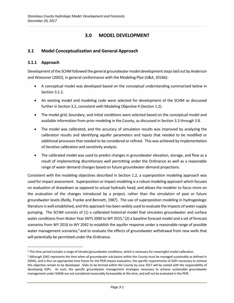
3.1.1 Approach
Development of the SCHM followed the general groundwater model development steps laid out by Anderson
and Woessner (2002), in general conformance with the Modeling Plan (JJ&A, 2016b):
• A conceptual model was developed based on the conceptual understanding summarized below in
Section 3.1.2.
• An existing model and modeling code were selected for development of the SCHM as discussed
further in Section 3.2, consistent with Modeling Objective 4 (Section 1.2).
• The model grid, boundary, and initial conditions were selected based on the conceptual model and
available information from prior modeling in the County, as discussed in Section 3.3 through 3.8.
• The model was calibrated, and the accuracy of simulation results was improved by analyzing the
calibration results and identifying aquifer parameters and inputs that needed to be modified or
additional processes that needed to be considered or refined. This was achieved by implementation
of iterative calibration and sensitivity analysis.
• The calibrated model was used to predict changes in groundwater elevation, storage, and flow as a
result of implementing discretionary well permitting under the Ordinance as well as a reasonable
range of water demand changes based on future groundwater demand projections.
Consistent with the modeling objectives described in Section 1.2, a superposition modeling approach was
used for impact assessment. Superposition or impact modeling is a robust modeling approach which focuses
on evaluation of drawdown as opposed to actual hydraulic head, and allows the modeler to focus more on
the evaluation of the changes introduced by a project, rather than the simulation of past or future
groundwater levels (Reilly, Franke and Bennett, 1987). The use of superposition modeling in hydrogeologic
literature is well established, and this approach has been widely used to evaluate the impacts of water supply
pumping. The SCHM consists of (1) a calibrated historical model that simulates groundwater and surface
water conditions from Water Year (WY) 2000 to WY 2015,5 (2) a baseline forecast model and a set of forecast
scenarios from WY 2016 to WY 2042 to establish the aquifer response under a reasonable range of possible
water management scenarios,6 and to evaluate the effects of groundwater withdrawal from new wells that
will potentially be permitted under the Ordinance.
5 This time period includes a range of climatic/groundwater conditions, which is necessary for meaningful model calibration. 6 Although 2042 represents the time when all groundwater sub-basins within the County must be managed sustainably as defined in SGMA, and is thus an appropriate time frame for the PEIR impact evaluation, the specific requirements of GSPs necessary to achieve this objective remain to be developed. GSAs to be formed within the County by June 2017 will be vested with the responsibility of developing GSPs. As such, the specific groundwater management strategies necessary to achieve sustainable groundwater management under SGMA are not considered reasonably foreseeable at this time, and will not be evaluated in the PEIR.

Stanislaus County Hydrologic Model: Development and Forecasts December 20, 2017
Page 3-2
3.1.2 Conceptual Understanding
The conceptual model for construction of the SCHM consists of the principal components summarized below.
• The area of interest for this study is the portion of the San Joaquin Valley Groundwater Basin that
underlies the County. This area includes all of the Modesto Subbasin and portions of the Eastern San
Joaquin and Delta Mendota Subbasins. In addition, all of the Turlock Subbasin, including portions
that lie in Merced County to the south, is included in the Study Area (Figure 2-1).
• Low permeability bedrock of the Sierra Nevada and the Diablo Range from the eastern and western
boundaries of the basin, respectively.
• A series of broad, coalescing alluvial fans along the western slope of the Sierra Nevada foothills
contain aquifers with unconfined to semi-confined conditions and represent a recharge zone
(forebay) for deeper confined aquifers closer to the center of the basin. In the eastern portion of this
area, Miocene fluvio-volcanic deposits of the Mehrten Formation contain productive aquifers, but
the presence of well-developed duripan soils limits local recharge.
• A narrow band of alluvial fans along the eastern margin of the Diablo Range behaves in a similar
fashion, functions as a region for local mountain-front recharge, and contains aquifers with
unconfined to semi-confined conditions.
• A central region with an upper unconfined to semi-confined aquifer system that is separated by the
Corcoran Clay from an underlying confined aquifer system underlies the center of the basin, where
deposits from the Sierra Nevada and the Coast Range interfinger.
• The freshwater-bearing valley-fill sediments are underlain by marine sedimentary deposits that
contain brackish water at depths between about 900 to 1,500 feet below ground surface.
• Groundwater-connected streams and rivers, including the Stanislaus, Tuolumne, and Merced Rivers,
enter the basin from the east and merge with the groundwater-connected San Joaquin River, which
flows northward along the valley axis. The Calaveras River crosses the northern triangle portion of
the SCHM.
• Reservoirs along the Stanislaus and Tuolumne River are located in the proximal alluvial fan areas near
the eastern margin of the basin.
• Groundwater flow, in the absence of groundwater pumping, is generally away from the Sierra Nevada
on the east and the Diablo Range on the west, toward the San Joaquin River in the center of the
valley, and northward along the San Joaquin River out of the County.
3.2 Modeling Code Selection
3.2.1 Available Models
Several existing groundwater flow models have been developed that cover all or portions of Stanislaus County
and are pertinent to the proposed modeling effort:

Stanislaus County Hydrologic Model: Development and Forecasts December 20, 2017
Page 3-3
• The Merced-Stanislaus (MERSTAN) model was developed by USGS in 2015, and covers portions of
three of the four groundwater subbasins in the County (Phillips, S.P. et al, 2015). It encompasses an
area of about 1,000 square miles centered on the Cities of Modesto and Turlock and was developed
using the MODFLOW-OWHM modeling code.
• The more generalized regional Central Valley Hydrologic Model (CVHM) developed by USGS includes
all of the groundwater subbasins in the County (USGS, 2009 and 2017). The current version of CVHM
was also developed using the MODFLOW-OWHM code and is currently being updated.
• The California Central Valley Groundwater-Surface Water Simulation Model (C2VSim) was developed
by DWR with the Integrated Water Flow Model (IWFM) code to evaluate groundwater and surface
water management issues in the Central Valley and delta (DWR, 2013b and 2016a). The model comes
in both a coarse grid version and a fine grid beta version, with the fine grid beta version improved to
support evaluation of groundwater flow at a local scale. The model is currently being updated and is
expected to be released in late 2017 or early 2018; however, some land use and other data utilized
for the updates have been made available by the DWR.
• A three-dimensional finite element model was prepared for the Turlock Subbasin by Timothy J.
Durbin as a consultant for TGBA and TID using a customized version of the FEMFLOW3D modeling
code (the TID Model) (Durbin, 2008). This model was recently used by TGBA for a study in the eastern
Turlock Subbasin. FEMFLOW3D is a proprietary modeling code.
• In support of its Aquifer Characterization and Recharge Project, the City of Modesto has developed a
city-wide groundwater flow model with the USGS MODFLOW code, using the GMS modeling
platform (the Modesto Model) (Todd and RMC, 2016). The model was extracted from the MERSTAN
model to evaluate groundwater flow on a more localized level. The underlying lithology and
discretization of the MERSTAN model were not changed.
3.2.2 Model and Code Selection
Consistent with the modeling objectives discussed in Section 1.2, the existing available models were
evaluated to determine if one of them could be used as a starting point for construction of the SCHM.
The MERSTAN, TID and Modesto models are not able, by themselves, to meet the modeling objectives, as
they do not cover all of Stanislaus County. In addition, the TID model is based on a proprietary modeling code
and therefore is not consistent with DWR guidance for development of models that would support GSPs
(DWR, 2016b). Data from these models may be used to refine the SCHM, but they were not considered
suitable as a starting point for model construction. The CVHM and the fine grid version of C2VSim (C2VSim-
FG) are both suitable starting points for development of a model that would meet the objectives discussed in
Section 1.2, and were evaluated in greater detail in the Modeling Plan (JJ&A, 2016a).
Although based on different modeling codes, C2VSim-FG and CVHM have many similarities, and use some of
the same data. Both models were constructed with the objectives of understanding the water budget of the
Central Valley, including groundwater/surface water interactions, irrigation demand, and changes in
groundwater levels and storage. In addition, both models provide a basis for continued investigations at the

Stanislaus County Hydrologic Model: Development and Forecasts December 20, 2017
Page 3-4
local scale via the development of “child” models based on regional “parent” analysis. Of these two models,
C2VSim was selected as the starting point for development of the SCHM for the following reasons:
• Planned use of C2VSim by DWR to evaluate the compliance of GSPs with the requirements of SGMA;
• It was anticipated that ongoing efforts by DWR would result in a greater level of support and beta
data availability than the CVHM;
• Compatibility with the CalSim and CalLite surface water models and related diversion data;
• Compatibility with groundwater modeling efforts to the north and south of the SCHM in San Joaquin
and Merced Counties, which are developing models based on the C2VSim modeling code, IWFM; and
• CVHM has limited options for pre- and post-processing tools that are publicly available; whereas,
several Excel and GIS pre- and post-processing tools are available for C2VSim.
When the decision was made to select C2VSim as the starting point for development of the SCHM, it was
expected that a calibrated update to the C2VSim-CG model would be released in early 2017, and an updated
beta version of C2VSim-FG would also be available. Both models were to be upgraded to the latest version
of the IWFM modeling code (IWFM version 2015), which includes several significant improvements over the
previous version, IWFM 3.02. Unfortunately, DWR’s updates of C2VSim took longer than originally
anticipated, and are now expected to be released in late 2017 or early 2018, as of the date of this report.
Therefore, the SCHM was constructed using the previously released beta version of C2VSim-FG, which is
based on the IWFM 3.02 modeling code and includes historical data through WY 2009. DWR was able to
make available several IWFM-formatted datasets, including updated precipitation data and land use data
based on updated crop surveys with data through WY 2015, which were able to be incorporated into
the SCHM.
3.3 Model Discretization
3.3.1 Finite Element Mesh
The finite element mesh for the SCHM was extracted from the C2VSim-FG model and is shown in Figure 2-1.
The mesh includes a total of 3,105 elements and 2,923 nodes, which average approximately 0.6 miles across
and range in size from 17 to approximately 1,500 acres within the SCHM domain. The extracted finite element
mesh for the SCHM covers Stanislaus County and the entirety of the Turlock Subbasin in Stanislaus and
Merced Counties. The mesh extends approximately 3 miles outside the boundaries of the primary model
area in order to provide a buffer zone that decreases the potential for boundary effects to influence model
results in the primary area of interest.
3.3.2 Water Budget Subregions
IWFM 3.02 utilizes water budget subregions for input of certain water budget data, including surface water
diversions and land use data (e.g., crop types). In order to accept updated land use data provided by DWR,

Stanislaus County Hydrologic Model: Development and Forecasts December 20, 2017
Page 3-5
the model domain was therefore subdivided in 108 subregions to correspond approximately with the C2VSim
coarse grid elements for which the land use data were provided. The subregions are shown graphically in
Figure 3-1.
3.3.3 Layering
The SCHM retained the layering scheme of the current C2VSim model, that is, a three-layer system with a
vertical conductance pseudo-layer to simulate the Corcoran Clay at the top of Model Layer 2. These layers
may be described as follows:
• Layer 1 extends from the ground surface to a depth of 202 to 1,005 feet, and represents the
uppermost unconfined to semi-confined aquifer system.
• Layer 2 underlies Layer 1 and ranges in thickness from 16 to 647 feet. It represents the semi-confined
to confined aquifer system that underlies the basin at depth to the east and west of the Corcoran
Clay subcrop area, and the lower, confined aquifer system below the Corcoran Clay.
• A vertical conductance pseudo-layer is defined at the top of Layer 2 to represent the Corcoran Clay.
The vertical conductance of the layer is defined by a hydraulic conductivity multiplied by a thickness,
which is set to the interpreted thickness of the Corcoran Clay where it is present, and to zero
(providing no impedance) where it is not. The extent of the Corcoran Clay layer is shown on Figure
3-2.
• Layer 3 underlies Layer 2 and represents a regional deep aquifer that ranges in thickness from 30 to
1,572 feet and overlies the interpreted base of fresh water in the area. This layer is penetrated by
few wells in the area, and its properties are therefore poorly documented.
3.4 Model Boundaries
The following boundary conditions were assigned, as shown in Figure 2-1:
• Similar to the C2VSim-FG model, the eastern and western boundaries of the model were designated
as no flow boundaries along the contact between the valley-fill alluvium and relatively impermeable
formations exposed in the foothills of the Sierra Nevada and the Diablo Range.
• The northern and southern model boundaries were designated as general-head boundaries, which
require designation of a general head and distance to the general head. Variable flow may occur
across these boundaries depending on variations in simulated hydraulic gradients over time. Time-
series head values for these boundaries were initially assigned based on heads extracted from beta
version of the C2VSim-FG model for WY 1991 to WY 2009. Boundary heads for WY 2010 to WY 2015
were duplicated from C2VSim data for years with similar hydrologic characteristics. These boundary
heads were updated during the model calibration process as discussed in Section 4.3.1.3. The
distance to the general heads was set at 1 meter.

Stanislaus County Hydrologic Model: Development and Forecasts December 20, 2017
Page 3-6
3.5 Sources and Sinks
Sources and sinks were modeled as follows:
• Rivers and streams, including Merced River, Orestimba Creek, Calaveras River, Stanislaus River and
Tuolumne River, were simulated using river nodes as shown in Figure 3-3. River boundary cells are a
head-dependent boundary condition that allows water to enter or exit the river according to the
head difference between the groundwater elevation and the surface water elevation, and in
proportion to the hydraulic conductivity and thickness of the stream bed layer, which is represented
by a conductance term. The stream bed conductance values from C2VSim were initially adopted for
use in the model, and updated during the calibration process as discussed in Section 4.3.3.
• Small watersheds that are tributary to the model were adopted from C2VSim and refined as
described in Section 3.9.3.3. They were further updated and refined during the calibration process
as described in Section 4.3.2.
• Reservoirs were simulated using recharge nodes with 100 percent recoverable losses (i.e., all seepage
losses remain within the model) in the footprints of the reservoirs shown in Figure 3-3. Additional
information regarding the assigned recharge rates at these nodes is provided in Section 3.9.3.4. The
diversion for Turlock Lake was adjusted during the calibration process to 33 percent recoverable and
67 percent non-recoverable losses.
• There are no tile drains in the current version of C2VSim within the domain of the SCHM. Tile drains
are reported to be located in some areas of shallow groundwater near the San Joaquin River within
TID; however, they are a relatively small component of the water budgets and information regarding
the drain depths and locations was not readily available, so they were not incorporated into the
model. These could be added at a later date if data regarding drain elevations and conductance
values is obtained.
• Municipal pumping wells were added based on data provided by municipal water agencies or
obtained from Urban Water Management Plans (UWMPs), Municipal Service Reviews (MSRs) and
other sources as described in Table 3-1. The locations of these wells are shown on Figure 3-4.
Additional information regarding development of the municipal pumping component of the model
groundwater budget is described in Section 3.9.4.1.
• Rural domestic pumping was evaluated using the methodology described in Section 3.9.4.2, and a
single surrogate well was defined in each of the 108 water-budget subregions in Layer 1 to simulate
this component of the regional groundwater demand. The locations of these wells are shown on
Figure 3-4.
• Recharge elements are designated in C2VSim to receive urban return flow, recoverable diversion
losses, and recharge from small watershed stream inflows. These nodes were retained, except that
recharge nodes for small watersheds were updated and refined during the model calibration process
as described in Section 4.3.2.

Stanislaus County Hydrologic Model: Development and Forecasts December 20, 2017
Page 3-7
3.6 Parameterization
The model was originally extracted with the aquifer parameter values assigned by C2VSim, which were then
updated as follows:
• Spatial data (xyz) regarding the distribution of hydraulic conductivity in the MERSTAN model were
extracted from that model and uploaded into the SCHM. Parameter data for the inactive portions of
the MERSTAN model west of the San Joaquin River were not used, as USGS staff indicated that the
data in this area were not subjected to the same level of geostatistical analysis as data east of the
river, and were therefore less reliable.7 The MERSTAN model includes 16 layers, which were assigned
as follows:
o Hydraulic conductivity values from MERSTAN Layers 1 through 7 were assigned to SCHM
Layer 1;
o Hydraulic conductivity values from MERSTAN Layer 8 represent the Corcoran Clay, and were
not used;
o Hydraulic conductivity values form MERSTAN Layers 9 through 13 were assigned to SCHM
Layer 2; and
o Hydraulic conductivity values from MERSTAN Layers 14 through 16 were assigned to SCHM
Layer 3
The hydraulic conductivities at each model node were calculated using the standard formulas for
calculation of effective vertical and lateral hydraulic conductivities of heterogeneous layered systems
as follows:
o Lateral hydraulic conductivity was calculated using the following formula:
𝑲𝒙 = ∑𝒌𝒊𝒅𝒊
𝒅𝒏𝒊=𝟏
o Vertical hydraulic conductivity was calculated using the following formula:
𝑲𝒛 = ∑𝒅𝒅𝒊𝑲𝒊
𝒏𝒊=𝟏
• Hydraulic conductivity data estimated from 30 specific capacity tests performed on wells in the
eastern foothills area of the County were used to update and adjust hydraulic conductivity values in
areas east of the MERSTAN model domain using a modified nearest-neighbor geospatial
analysis technique.
• Hydraulic conductivity data estimated from 23 specific capacity and aquifer pumping tests west of
the San Joaquin River were similarly used to update and adjust hydraulic conductivity values in that
area using a modified nearest neighbor geospatial analysis technique.
7 Steve Phillips, USGS, personal communication, July 2017.

Stanislaus County Hydrologic Model: Development and Forecasts December 20, 2017
Page 3-8
• The vertical hydraulic conductivity and thickness of the Corcoran Clay were used to calculate the
conductance term assigned to aquitard at the top of Layer 2. To do this, the lateral extent and
thickness of the Corcoran Clay reported by the USGS was used (USGS, 2012), as shown in Figure 3-2.
The vertical hydraulic conductivity of the Corcoran Clay within the SCHM is not well characterized,
but a reasonable range based on the literature is approximately 6.2 x 10⁻⁴ to 3.0 x 10⁻⁶ ft/day (USGS,
2004b; USGS, 2009). A uniform vertical hydraulic conductivity of 1 x 10⁻⁵ feet/day was applied to the
Corcoran Clay based on these values, and then adjusted as appropriate during calibration as
discussed in Section 4.3.5.
• Targeted changes to the initial lateral and vertical hydraulic conductivity assignments were made
during the calibration process as described in Section 4.3.4.
• The SCHM retained the aquifer specific yield, specific storage, elastic and inelastic storage
coefficients, interbed thickness, minimum interbed thickness, and precompaction hydraulic head
incorporated in C2VSim.
To help illustrate the above described parameterization process, the initial distribution of lateral hydraulic
conductivity in SCHM Layer 1 in relation to the MERSTAN model domain, and the locations of wells for which
hydraulic conductivity data were calculated is shown in Figure 3-5.
3.7 Model Time Period
The Ordinance was adopted in November of 2014, and the primary period of interest to be evaluated using
the SCHM covers the time that discretionary well permits will be issued in unincorporated, non-district lands
prior to adoption of GSPs. Adoption and implementation of GSPs will take place in the Delta Mendota and
Eastern San Joaquin Subbasins beginning in 2020, and in the Modesto and Turlock Subbasins beginning in
2022. Achievement of sustainable groundwater management is required throughout the basins within 20
years after GSPs are adopted, or in 2040 and 2042, respectively. During this time, wells determined by the
County to be operated unsustainably may be regulated under the Ordinance.
Based on this information, the temporal simulation periods of the model may be subdivided as shown
graphically in Figure 3-6 and as described below:
• A model “warm up period” was established from WY 1991 to WY 1999 to allow the model to reach
conditions that are consistent with historical water budget inputs;
• A calibration or history matching period of WY2000 to WY2015 was selected, and includes a selection
of wet, dry and normal hydrologic years to allow for a robust calibration process;
• A forecast period extending from WY 2016 to WY 2042 was established to run forward simulations
capable of assessing reasonably foreseeable water management and climatic trends, and evaluating
the impacts of issuing discretionary well permits under the Ordinance.

Stanislaus County Hydrologic Model: Development and Forecasts December 20, 2017
Page 3-9
Figure 3-6: Timeline for Well Permitting Requirements Evaluated in the SCHM
3.8 Initial Conditions
Starting heads for the model were initially extracted for October of 1990 (the beginning of WY 1991) after
running the existing version of C2VSim from 1921 to 1990. The use of a warmup period makes the model less
sensitive to the choice of initial heads. Nevertheless, after the water budget adjustments during the
calibration process (Section 4.3.1), WY 1999 model heads were substituted as the initial WY 1991 heads
because these were generally more closely aligned with observed heads as seen in the calibration wells
reported for the model warmup period (WY 1991 to WY 1999). Historical Water Budget Data
Water budget data for the model calibration (history match) period were compiled from several sources
as follows:
• The water budget data from C2VSim-FG were initially retained in the SCHM and updated when more
reliable data were deemed to be available;
• Updated land use and precipitation data from WY 1991 through WY 2015 were provided by DWR
from its work in updating C2VSim and were incorporated into the SCHM;
• Municipal water budget data provided by municipal water purveyors and/or data from UWMPS,
MSRs and other plans and reports were incorporated into the model as described in Table 3-1 and in
Sections 3.9.4.1;
• Diversion data from C2VSim were re-allocated from the six water budget subregions defined in
C2VSim to the 108 water budget subregions defined in the SCHM, and updated based on information
provided by agricultural water purveyors and/or data from Agricultural Water Management Plans
(AWMPs), MSRs and other plans and reports as described in Table 3-2 and in Section 4.3.1.1;
19
90
- - - -1
99
5- - - -
20
00
- - - -2
00
5- - - -
20
10
- - - -2
01
5- - - -
20
20
- - - -2
02
5- - - -
20
30
- - - -2
03
5- - - -
20
40
-2
04
2
WATER YEAR
Model Warmup
Period
Model Calibration Period
Model Forecast Period
OrdinanceAdopted
GSPsAdopted
Discretionary Well Permitting
Discretionary Regulation of Unsustainable Wells

Stanislaus County Hydrologic Model: Development and Forecasts December 20, 2017
Page 3-10
• Agricultural land use and water budget data provided by agricultural water purveyors and/or data
from AWMPs, MSRs and other plans and reports were used as described in Table 3-3 to refine model
cropping data, the diversions listed in Table 3-2 and the diversion recoverable and non-recoverable
losses (Table 3-4), allocation loss and cropping data as further described in Sections 3.9.4.3 and
4.3.1.2;
• Agricultural land use data provided by the Stanislaus County Agricultural Commissioner for non-
district areas in the eastern portion of the SCHM were incorporated during the model calibration
process as described in Section 4.3.1.2;
• Small watershed recharge locations and rates were refined to scale small watersheds split across the
model boundaries, and were adjusted during the calibration process as discussed in Section 4.3.2;
• Stream inflows were updated for WY 2010 through WY 2015 using gaging station data; and
• River conductance values were adjusted to change the surface-groundwater interaction in some
reaches during the calibration process as discussed in Section 4.3.3.
3.8.1 Precipitation
Updated precipitation data were obtained from DWR for WY 1991 through WY 2015 in a gridded dataset that
was applied to the 108 water-budget subregions defined in the SCHM. The data were derived by DWR using
the Parameter-elevation Regressions on Independent Slopes Model (PRISM), which is a climate analysis
system that uses point data, a digital elevation model (DEM), and other spatial datasets to generate gridded
estimates of annual, monthly and event-based climatic parameters (Daly et al., 1997 and 2004).
3.8.2 Stream Inflows
The major stream inflows into the SCHM were developed as follows:
• River inflows (Rim Inflows) for the Stanislaus River, Tuolumne River, Merced River, Calaveras River,
and Orestimba Creek were adopted from C2VSim for WY 1991 through WY 2009, and derived from
the USGS gaging station flow data for the C2VSim-assigned gaging stations for WY 2010 through WY
2015; and
• River inflows for the San Joaquin River were defined using the C2VSim river node at the river’s entry
point into the SCHM for WY 1991 through WY 2009; for WY 2010 through WY 2015, inflows were
extrapolated based on USGS gaging station data for the San Joaquin River at Newman which were
scaled based on pre-2010 correlation with the SCHM inflow data.
3.8.3 Recharge
Recharge, or deep percolation, is calculated in IWFM 3.02 by routing excess water from land surface processes
such as land use (agricultural, urban, native vegetation or riparian), precipitation, irrigation, conveyance
losses, runoff, return flow and surface water, as infiltration into a root-zone model, from which it is routed
downward through the vadose zone model and into groundwater based on soil moisture content and field
Stanislaus County Hydrologic Model: Development and Forecasts December 20, 2017
Page 3-11
capacity (or directly into groundwater when it is shallow enough) (DWR, 2013c). The land surface, root zone
and vadose zone processes are controlled by a number of sub-processes, water budget and soil property
variables that can be defined in the model input files. The reader is referred to the document DWR 2013b for
a more complete discussion regarding the model’s approach to the generation and routing of recharge.
3.8.3.1 Areal Recharge from Precipitation
Areal infiltration into the root zone in IWFM 3.02 is calculated on a subregional level based on precipitation,
soil properties and designated elemental land use. Precipitation inputs into the SCHM were updated based
on data provided by the DWR as described in Section 3.9.1. The remaining factors used by the surface and
land use processes, root zone model and vadose zone model to calculate areal recharge were adopted
unchanged from C2VSim.
3.8.3.2 Streams
Recharge from streams (or discharge to streams) in IWFM 3.02 is governed by defined streambed geometry
and conductance terms at each stream node, stream flows and the surface and groundwater hydrology
modeled at the stream (i.e., whether the stream is gaining, losing, or disconnected from direct
groundwater interaction). Stream flows in the SCHM were simulated as discussed in Section 3.9.2.
The conductance terms consist of a streambed thickness and hydraulic conductivity.
Streambed conductance values in C2VSim were adopted in the SCHM, and then adjusted for some reaches
as discussed in Section 4.3.3.
3.8.3.3 Small Watersheds
Inflow into the model from tributary watersheds that are not modeled as streams is simulated in IWFM using
“small watersheds” for which runoff, underflow in, and recharge at designated recharge nodes are simulated.
C2VSim includes 18 small watersheds that are tributary to the SCHM, some of which are also tributary to
portions of C2VSim that fall outside the SCHM model domain. The input data for the overlapping small
watersheds was scaled based on the portion of the watersheds tributary to the SCHM model domain, and
the C2VSim data for the small watersheds was adopted unchanged into the SCHM. Changes to the number
of specifications of recharge nodes for some of the small watersheds were made during the calibration
process as described in Section 4.3.2.
3.8.3.4 Reservoirs
Three reservoirs in the eastern Stanislaus County serve to provide off-stream storage for water to be delivered
for agricultural and municipal use: Modesto Reservoir and Turlock Lake, which receive water diverted from
the Tuolumne River, and Woodward Reservoir, which receives water diverted from the Stanislaus River.
These reservoirs are located in the low foothills of the Sierra Nevada near the contact between the Mehrten
and Turlock Lake Formations, which include relatively permeable sands, and the reservoirs therefore are a
significant source of local recharge. C2VSim does not simulate these reservoirs, so they were added by

Stanislaus County Hydrologic Model: Development and Forecasts December 20, 2017
Page 3-12
designating recharge nodes with 100 % recoverable losses (i.e., all of the water stays within the model) within
the footprints of the reservoirs that receive water imports from outside the model in proportion to the
estimated seepage losses, as described in Section 3.5. Losses for Turlock Lake were adjusted during the
calibration process. Recharge from these reservoirs was estimated using the following approach:
• Annual seepage losses from Woodward Reservoir from 1994 through 2014 were taken from a water
balance table provided in the 2015 AWMP for South San Joaquin Irrigation District (SSJID) (Davids
Engineering, 2015). Values for 1990 to 1993 and 2015 were substituted from similar hydrologic years
in the available record. In the absence of specific data, seepage was assumed to be a constant value
during each month of any given year.
• Monthly seepage losses for Turlock Lake were calculated from lake inflow, outflow and storage data
provided by TID, subtracting evaporation losses. Evaporation losses were calculated by scaling
annual evaporation losses reported for Woodward Reservoir (Davids Engineering, 2015) based on
the relative size of the free water surface areas of the reservoirs at average high-water levels,
distributed based on reported monthly potential evapotranspiration.
• Monthly seepage losses for Modesto Reservoir were calculated from lake inflow and outflow data
provided by Modesto Irrigation District, and storage data from California Data Exchange Center
(CDEC), subtracting evaporation losses. Evaporation losses were calculated by scaling annual
evaporation losses reported for Woodward Reservoir (Davids Engineering, 2015) based on the
relative size of the free water surface areas of the reservoirs at average high-water levels, distributed
based on reported monthly potential evapotranspiration.
3.8.3.5 Urban Deep Percolation
Urban deep percolation is derived from diversion conveyance losses, urban landscape irrigation, wastewater
return flows and precipitation. Infiltration into the root zone model is controlled by a number of factors that
can be defined in the model inputs (indoor vs. outdoor water use fractions, urban evapotranspiration, percent
of impervious materials, designated return flow and recharge fractions, etc.). From the root zone model,
infiltration is routed through a vadose zone model and into groundwater depending on soil properties and
antecedent moisture conditions. Urban deep percolation as a function of urban supply therefore varies from
year to year in the model. Refining these variables was beyond the scope of this project. They were therefore
adopted unchanged from C2VSim, and could be refined during future modeling efforts.
3.8.3.6 Agricultural Deep Percolation
Similar to urban deep percolation, agricultural deep percolation is calculated by the model based on a
complex series of interactions between land use, water supply, evapotranspiration, irrigation efficiency,
drainage, applied water and soil conditions. Similar to urban deep percolation, agricultural infiltration is
routed from the root zone model through a vadose zone model and into groundwater depending on soil
properties and antecedent moisture conditions. Agricultural deep percolation as a function of applied water
therefore varies by location and from year to year in the model. Refining these variables was beyond the

Stanislaus County Hydrologic Model: Development and Forecasts December 20, 2017
Page 3-13
scope of this project. They were therefore adopted unchanged from C2VSim, and could be refined during
future modeling efforts. WALT: Same comment applies here.
3.8.4 Pumpage
3.8.4.1 Municipal Pumping
Municipal pumping in IWFM 3.02 can either be designated by entering pumping well specifications or by
entering a municipal demand and allowing the model to calculate pumping based on the difference between
available surface water diversions and demand. C2VSim identified centrally located surrogate wells for each
urban area to simulate municipal groundwater pumping. For the SCHM, municipal pumping was specified by
entering well data. The approach used is summarized in Table 3-1 and included the following steps:
• The locations of 218 municipal wells reported by municipal water purveyors or identified from
UWMPs, MSRs or other planning documents were entered into the model;
• Completion depths and screen intervals were added for the wells when available, or were estimated
based on nearby supply wells when they were not available;
• The locations and completion details of four surrogate wells used in C2VSim to simulate municipal
groundwater pumping in four cities located within the buffer zone outside the primary model area
(Escalon, Ripon, Gustine and Livingston) were retained; and
• Annual and monthly municipal groundwater pumping was specified based on information reported
by municipal water purveyors, and/or data from UWMPs, MSRs or other planning documents,
augmented by information regarding population trends, as summarized in Table 3-1.
3.8.4.2 Rural Domestic Pumping
Rural domestic pumping was assumed to occur from Model Layer 1 and was estimated using the following
geospatial analysis approach:
• Rural domestic pumping was assumed to occur in each water budget subregion with land falling
outside the cities and community service districts included in the SCHM;
• The intersection between the areas identified as having rural domestic water demand and Census
2000 tracts was used to estimate the number of households reliant on rural domestic pumping for
their water supply in that year;
• A default water demand of 0.5 acre-feet per year (AFY) was assumed for each rural domestic
household (Water Research Foundation, 2016), and was decreased by 38% to account for return
flows from landscape irrigation and wastewater disposal to septic systems (Aquacraft, 2011); and
• The rural domestic water demand was adjusted for the model period prior to and following 2000
based on rural population trends reported in the Stanislaus County General Plan Housing Element
(Michael Baker International, 2016).

Stanislaus County Hydrologic Model: Development and Forecasts December 20, 2017
Page 3-14
3.8.4.3 Agricultural Pumping
Agricultural pumping is calculated by IWFM 3.02 based on the difference between the total irrigation water
demand and the amount of surface water and precipitation available to meet the demand. The resulting
agricultural pumpage is applied on an elemental basis. The irrigation water demand is calculated by the
model for each subregion based on designated land use, crop type, evapotranspiration, irrigation efficiency
and soil properties. The following approach was used to calculate agricultural pumping in the SCHM:
• Land use data from DWR crop surveys was provided by DWR through WY 2015 and entered into the
input files for each SCHM subregion;
• Crop types were adjusted from C2VSim/IWFM 2015 data (which is the format provided by DWR) to
correlate with the crop types available in C2VSim/IWFM 3.02;
• Evapotranspiration, irrigation efficiencies, and soil properties were adopted unchanged
from C2VSim;
• Diversions and diversion losses were determined based on data provided by irrigation districts or
available from AWMPs, MSRs and various planning documents using the process described in Tables
3-2, 3-3 and 3-4; and
• Diversions, diversion losses and crop data were adjusted during the calibration process based on
comparison between modelled and reported farm gate water deliveries and groundwater pumping
as described in Table 3-3 and Section 4.3.1.1.
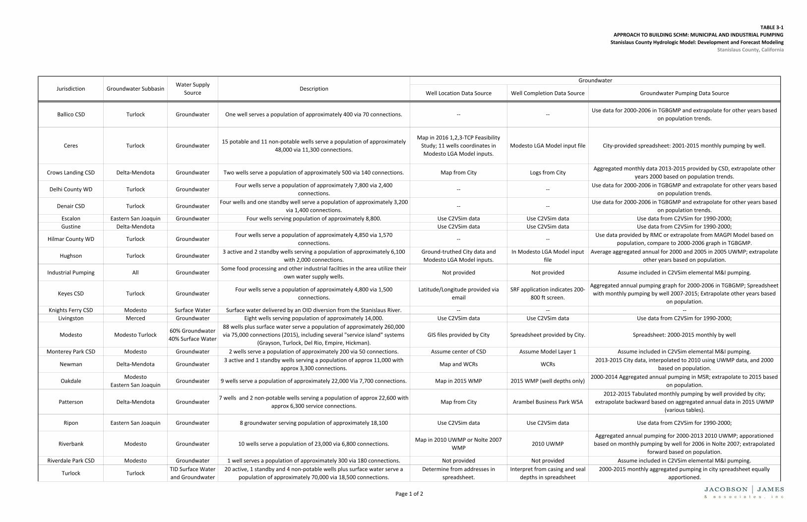
TABLE 3‐1APPROACH TO BUILDING SCHM: MUNICIPAL AND INDUSTRIAL PUMPING
Stanislaus County Hydrologic Model: Development and Forecast ModelingStanislaus County, California
Well Location Data Source Well Completion Data Source Groundwater Pumping Data Source
Ballico CSD Turlock Groundwater One well serves a population of approximately 400 via 70 connections. ‐‐ ‐‐Use data for 2000‐2006 in TGBGMP and extrapolate for other years based
on population trends.
Ceres Turlock Groundwater 15 potable and 11 non‐potable wells serve a population of approximately
48,000 via 11,300 connections.
Map in 2016 1,2,3‐TCP Feasibility Study; 11 wells coordinates in Modesto LGA Model inputs.
Modesto LGA Model input file City‐provided spreadsheet: 2001‐2015 monthly pumping by well.
Crows Landing CSD Delta‐Mendota Groundwater Two wells serve a population of approximately 500 via 140 connections. Map from City Logs from CityAggregated monthly data 2013‐2015 provided by CSD, extrapolate other
years 2000 based on population trends.
Delhi County WD Turlock GroundwaterFour wells serve a population of approximately 7,800 via 2,400
connections.‐‐ ‐‐
Use data for 2000‐2006 in TGBGMP and extrapolate for other years based on population trends.
Denair CSD Turlock GroundwaterFour wells and one standby well serve a population of approximately 3,200
via 1,400 connections.‐‐ ‐‐
Use data for 2000‐2006 in TGBGMP and extrapolate for other years based on population trends.
Escalon Eastern San Joaquin Groundwater Four wells serving population of approximately 8,800. Use C2VSim data Use C2VSim data Use data from C2VSim for 1990‐2000; Gustine Delta‐Mendota Use C2VSim data Use C2VSim data Use data from C2VSim for 1990‐2000;
Hilmar County WD Turlock GroundwaterFour wells serve a population of approximately 4,850 via 1,570
connections.‐‐ ‐‐
Use data provided by RMC or extrapolate from MAGPI Model based on population, compare to 2000‐2006 graph in TGBGMP.
Hughson Turlock Groundwater3 active and 2 standby wells serving a population of approximately 6,100
with 2,000 connections.Ground‐truthed City data and Modesto LGA Model inputs.
In Modesto LGA Model input file
Average aggregated annual for 2000 and 2005 in 2005 UWMP; extrapolate other years based on population.
Industrial Pumping All GroundwaterSome food processing and other industrial facilties in the area utilize their
own water supply wells.Not provided Not provided Assume included in C2VSim elemental M&I pumping.
Keyes CSD Turlock GroundwaterFour wells serve a population of approximately 4,800 via 1,500
connections.Latitude/Longitude provided via
emailSRF application indicates 200‐
800 ft screen.
Aggregated annual pumping graph for 2000‐2006 in TGBGMP; Spreadsheet with monthly pumping by well 2007‐2015; Extrapolate other years based
on population.Knights Ferry CSD Modesto Surface Water Surface water delivered by an OID diversion from the Stanislaus River. ‐‐ ‐‐ ‐‐
Livingston Merced Groundwater Eight wells serving population of approximately 14,000. Use C2VSim data Use C2VSim data Use data from C2VSim for 1990‐2000;
Modesto Modesto Turlock60% Groundwater 40% Surface Water
88 wells plus surface water serve a population of approximately 260,000 via 75,000 connections (2015), including several "service island" systems
(Grayson, Turlock, Del Rio, Empire, Hickman).GIS files provided by City Spreadsheet provided by City. Spreadsheet: 2000‐2015 monthly by well
Monterey Park CSD Modesto Groundwater 2 wells serve a population of approximately 200 via 50 connections. Assume center of CSD Assume Model Layer 1 Assume included in C2VSim elemental M&I pumping.
Newman Delta‐Mendota Groundwater3 active and 1 standby wells serving a population of approx 11,000 with
approx 3,300 connections.Map and WCRs WCRs
2013‐2015 City data, interpolated to 2010 using UWMP data, and 2000 based on population.
OakdaleModesto
Eastern San JoaquinGroundwater 9 wells serve a population of approximately 22,000 Via 7,700 connections. Map in 2015 WMP 2015 WMP (well depths only)
2000‐2014 Aggregated annual pumping in MSR; extrapolate to 2015 based on population.
Patterson Delta‐Mendota Groundwater7 wells and 2 non‐potable wells serving a population of approx 22,600 with
approx 6,300 service connections.Map from City Arambel Business Park WSA
2012‐2015 Tabulated monthly pumping by well provided by city; extrapolate backward based on aggregated annual data in 2015 UWMP
(various tables).
Ripon Eastern San Joaquin Groundwater 8 groundwater serving population of approximately 18,100 Use C2VSim data Use C2VSim data Use data from C2VSim for 1990‐2000;
Riverbank Modesto Groundwater 10 wells serve a population of 23,000 via 6,800 connections.Map in 2010 UWMP or Nolte 2007
WMP2010 UWMP
Aggregated annual pumping for 2000‐2013 2010 UWMP; apporationed based on monthly pumping by well for 2006 in Nolte 2007; extrapolated
forward based on population.Riverdale Park CSD Modesto Groundwater 1 well serves a population of approximately 300 via 180 connections. Not provided Not provided Assume included in C2VSim elemental M&I pumping.
Turlock TurlockTID Surface Water and Groundwater
20 active, 1 standby and 4 non‐potable wells plus surface water serve a population of approximately 70,000 via 18,500 connections.
Determine from addresses in spreadsheet.
Interpret from casing and seal depths in spreadsheet
2000‐2015 monthly aggregated pumping in city spreadsheet equally apportioned.
GroundwaterWater Supply
SourceJurisdiction DescriptionGroundwater Subbasin
Page 1 of 2

TABLE 3‐1APPROACH TO BUILDING SCHM: MUNICIPAL AND INDUSTRIAL PUMPING
Stanislaus County Hydrologic Model: Development and Forecast ModelingStanislaus County, California
Well Location Data Source Well Completion Data Source Groundwater Pumping Data Source
GroundwaterWater Supply
SourceJurisdiction DescriptionGroundwater Subbasin
Waterford Modesto GroundwaterThree systems serve a population of approximately 10,000: Two adjacent systems (Waterford and River Pointe) with 8 wells serve 2,400 connections;
Hickman with 2 wells serves 180 connections.Maps in 2016 WMP 2016 WMP Well depth table Calculate from data in 2016 WMP and extrapolate based on population.
Westley CSD Delta‐Mendota GroundwaterGroundwater purchased from Hillview Homes: 2 wells serve a population
of approximately 70.NA NA Assume included in C2VSim elemental M&I pumping.
Notes:C2VSim = California Central Valley Groundwater‐Surface Water Simulation ModelCSD = Community Services Districtft = footGIS = geographic information systemKMZ = keyhole markup language (geographic annotation for two‐dimensional maps and three‐dimensional Earth browsers)LGA = Local Groundwater AssistanceMAGPI = Merced Area Groundwater Pool InterestM&I = municipal and industrialMSR = Municipal Service ReviewRMC = RMC Water and EnvironmentSRF = Safe Drinking Water State Revolving Fund1,2,3‐TrichloropropaneTGBGMP = Turlock Groundwater Basin Groundwater Management PlanTID = Turlock Irrigation DistrictUWMP = Urban Water Management PlanWCR = well completion reportWD = Water DistrictWMP = Water Master PlanWSA = Water Supply Assessment% = percent‐‐ = not available/not applicable
References:City of Patterson, 2012. Water Supply Assessment for Arambel Business Park/KDN Retail Center Final Draft. April. Nolte Associates, Inc., 2007. City of Riverbank Water Supply Study and Water Master Plan. Volume I. Prepared for City of Riverbank. November. Provost & Pritchard Consulting Group, 2016. City of Ceres 1,2,3‐TCP Mitigation Feasibiilty Study. Prepared for City of Ceres. August 22.
Page 2 of 2

TABLE 3‐2SCHM HISTORICAL AND FORECAST DIVERSIONS
Stanislaus County Hydrologic Model: Development and Forecast ModelingStanislaus County, California
C2VSim Diversion ID
SCHM Diversion ID
C2VSim Diversion NameWater District(s)/Area Receiving
Water DeliveriesApproach for Calculating Diversions for Historical Model Period
(WY1990 ‐ WY2015)Approach for Calculating Diversions for Forecast Model Period (WY2016 ‐ WY2042)
85 1 Calaveras River SEWD
Use reported diversions from New Hogan Reservoir for 2013‐2015 in Table 7 of the SEWD AWMP. For 1990‐2012, calculate the fraction of the 2014 Diversion 85 volume in each year, and multiply it by the 2014 delivery reported in the AWMP. Multiply all diversions by 0.09 based on the percentage of the SEWD service territory within the model domain.
Calculate monthly delivery fraction using reported average monthly deliveries reported for OID.
Use historical year data in the order specified in Table 3. For historical years 1983‐1987, use years of the same hydrologic year type from the historical model dataset (1995, 1996,
2004, 2005 and 1990, respectively).
93 2Sacramento‐San Joaquin Delta to
SWPOak Flat Water District
Use reported 2006 ‐ 2015 diversions reported in 2016 Municipal Service Review. Calculate 1990‐2005 diversions by multiplying the maximum district allocation by reported historical SWP deliveries. Calculate monthly delivery fraction
using reported average deliveries reported for DPWD.
Use historical year data in the order specified in Table 3. For historical years 1983‐1987, use years of the same hydrologic year type from the historical model dataset (1995, 1996,
2004, 2005 and 2007, respectively).
94 3Stanislaus River to South San Joaquin
Canal for AgricultureSEWD
Use reported diversions from New Melones Reservoir for 2013‐2015 in Table 7 of the SEWD AWMP. For 1990‐2012,calculate the fraction of the 2014 Diversion 85 volume in each year, and multiply it by the 2014 delivery reported in
the AWMP. Multiply all diversions by 0.09 based on the percentage of the SEWD service territory within the model domain. Calculate monthly delivery fraction using reported average monthly deliveries reported for OID.
Use historical year data in the order specified in Table 3. For historical years 1983‐1987, use years of the same hydrologic year type from the historical model dataset (1995, 1996,
2004, 2005 and 2007, respectively).
94 3Stanislaus River to South San Joaquin
Canal for AgricultureSSJID
Use reported 1994‐2014 releases from Woodward Reservoir in Table 14 of the SSJID AWMP. For 1990‐1993 and 2015, calculate the fraction of the 2014 Diversion 94 volume in each year, and multiply it by the 2014 delivery reported in the AWMP. Multiply all diversions by 0.51 based on the percentage of the SSJID service territory within the model domain.
Calculate monthly delivery fraction using reported average monthly deliveries reported for OID.
Use historical year data in the order specified in Table 3. For historical years 1983‐1987, use years of the same hydrologic year type from the historical model dataset (1995, 1996,
2004, 2005 and 2007, respectively).
95 4Stanislaus River to South San Joaquin
Canal for M&ICity of Ripon
Use 0 for 1990‐1998, 0.5 TAF for 1999‐2005, 1 TAF for 2006‐2010, 1.5 TAF for 2011‐2015. Calculate monthly delivery fraction using reported average monthly deliveries reported for OID.
Use historical year data in the order specified in Table 3. For historical years 1983‐1987, use 0.
96 5Stanislaus River to Oakdale Canal for
AgricultureOID
Use data from OID‐provided spreadsheet "OID Hist Use ‐ DW & Surface H2O_1990 to 2016.xls", adjusted for 98% of service territory in SCHM. Calculate monthly delivery fraction using reported average monthly deliveries reported for OID.
Use historical year data in the order specified in Table 3. For historical years 1983‐1987, use years of the same hydrologic year type from the historical model dataset (1995, 1996,
2004, 2005 and 2007, respectively).
98 6Stanislaus River riparian for
AgricultureNon‐district parcels near Stanislaus
RiverUse C2VSim diversions unchanged. Use historical C2VSim Diversion 98 data in the order specified in Table 3.
100 7 Tuolumne River to Modesto CanalPrimary diversion to Modesto
Reservoir for Modesto Irrigation District and City of Modesto
Use C2VSim diversions multiplied by 0.93 to match reported farm gate deliveries for Diversion 101 and reasonable losses. Use historical C2VSim Diversion 100 data in the order specified in Table 3, multiplied by
0.93.
101 8 Modesto Canal for Agriculture Modesto Irrigation DistrictCalculate based on difference between adjused Diversion 100 after lossses minus Diversion 102 ([Diversion 100 x 0.93] ‐
Diversion 102). Calculate monthly delivery fraction using reported average monthly deliveries reported for OID.
Use historical year data in the order specified in Table 3. For historical years 1983‐1987, use years of the same hydrologic year type from the historical model dataset during
which surface water deliveries were made (1995, 1996, 2004, 2005, and 2007, respectively).
102 9 Modesto Canal for M&I City of ModestoUse 2000‐2015 "MID" data from City‐provided spreadsheet titled "Modesto Monthly system flow totals 2000‐2017.xls" and multiply by 1.06. For 1995 to 1999, use 35,616. For 1994, use 15,710. Assume constant puming rate throughout
each year.
Use historical year data in the order specified in Table 3. For historical years 1983‐1987, use years of the same hydrologic year type from the historical model dataset during
which surface water deliveries were made (1995, 1996, 2004, 2005, and 2007, respectively).
103 10Tuolumne River right bank riparian
diversions for AgricultureNon‐district parcels near Tuolumne
River right bankUse C2VSim monthly diversions unchanged. Use historical C2VSim data in the order specified in Table 3.
105 11Tuolumne River left bank riparian
diversions for AgricultureNon‐district parcels near Tuolumne
River left bankUse C2VSim monthly diversions unchanged. Use historical C2VSim data in the order specified in Table 3.
107 12 Tuolumne River to Turlock CanalPrimary diversion to Turlock Lake for
TIDUse C2VSim Diversion 107 multiplied by 0.90. Use adjusted historical C2VSim Diversion 107 data in the order specified in Table 3.
108 13 Turlock Canal for Agriculture TID Use unadjusted C2VSim Diversion 107 minus 13%. Distribute in proportional to farm gate delivery data provided by TID. Use adjusted historical C2VSim Diversion 107 data in the order specified in Table 3.
110 14Merced River to Merced ID Northside
Canal for AgricultureMerced Irrigation District north of
Merced River
Use 2010 to 2015 data from Table 5‐15 in the Merced ID AWMP multiplied by the fraction of the Merced ID service territory located north of the Merced River. Apply average monthly OID delivery fractions. For 1990 to 2009, use C2VSim
monthly diversions unchanged.
Use historical year data in the order specified in Table 3. For historical years 1983‐1987, use years of the same hydrologic year type from the historical model dataset (1995, 1996,
2004, 2005 and 2007, respectively).
Page 1 of 3

TABLE 3‐2SCHM HISTORICAL AND FORECAST DIVERSIONS
Stanislaus County Hydrologic Model: Development and Forecast ModelingStanislaus County, California
C2VSim Diversion ID
SCHM Diversion ID
C2VSim Diversion NameWater District(s)/Area Receiving
Water DeliveriesApproach for Calculating Diversions for Historical Model Period
(WY1990 ‐ WY2015)Approach for Calculating Diversions for Forecast Model Period (WY2016 ‐ WY2042)
112 15Merced River right bank riparian
diversions for AgricultureNon‐district parcels near Merced
River right bankUse C2VSim monthly diversions unchanged. Use historical C2VSim data in the order specified in Table 3.
114 16Merced River left bank riparian
diversions for AgricultureNon‐district parcels near Merced
River left bankUse C2VSim monthly diversions unchanged. Use historical C2VSim data in the order specified in Table 3.
116 17Merced River to Merced ID Main
Canal for AgricultureMerced Irrigation District south of
Merced River
Use 2010 to 2015 data from Table 5‐15 in the Merced ID AWMP multiplied by the fraction of the Merced ID service territory located south of the Merced River, plus Stevinson Water District deliveries. Apply average monthly OID delivery
fractions. For 1990 to 2009, use C2VSim monthly diversions unchanged. Apply Stevinson Water District diversion to model subregion that corresponds with their territory.
Use historical year data in the order specified in Figure 6‐1. For historical years 1983‐1987, use years of the same hydrologic year type from the historical model dataset (1995,
1996, 2004, 2005 and 2007, respectively).
128 18San Joaquin River riparian diversions,
Fremont Ford to Vernalis, to Subregion 10 for Agriculture
Non‐district parcels near San Joaquin River left bank
Assume same as right bank diversions, which are C2VSim Diversion 129 + Diversion 130.Use historical year data in the order specified in Figure 6‐1 For historical years 1983‐
1987, use years of the same hydrologic year type from the historical model dataset (1995, 1996, 2004, 2005 and 2007, respectively).
128 18San Joaquin River riparian diversions,
Fremont Ford to Vernalis, to Subregion 10 for Agriculture
PIDUse 2001 to 2010 data from the "Local Water" column in Table 8 of the PID AWMP. For 1990 to 2000 and 2011 to 2013, use the 2001‐2010 average. For 2014 and 2015, use half the average. Apply monthly delivery fractions reported in the
2008 DPWD AWMP.
Use historical year data in the order specified in Figure 6‐1 For historical years 1983‐1987, use years of the same hydrologic year type from the historical model dataset (1995,
1996, 2004, 2005 and 2007, respectively).
128 18San Joaquin River riparian diversions,
Fremont Ford to Vernalis, to Subregion 10 for Agriculture
El Solyo Water DistrictFor 2008‐2015, use EWRIMS data. For 1990 to 2007, use average of 2008 to 2013 EWRIMS data. Apply monthly delivery
fractions reported in the 2008 DPWD AWMP.
Use historical year data in the order specified in Figure 6‐1 For historical years 1983‐1987, use years of the same hydrologic year type from the historical model dataset (1995,
1996, 2004, 2005 and 2007, respectively).
128 18San Joaquin River riparian diversions,
Fremont Ford to Vernalis, to Subregion 10 for Agriculture
West San Joaquin Irrigation DistrictFor 2012 to 2015, use diversion data from WSID tab of comparison spreadsheet (J31:J34). For 1990 to 2011, refer "WSID
Reports 2015.xls" in the data library. In the Water Delivery tab: From Total Diverted, subtract CVP. Apply monthly delivery fractions reported in the 2008 DPWD AWMP.
Use historical year data in the order specified in Figure 6‐1 For historical years 1983‐1987, use years of the same hydrologic year type from the historical model dataset (1995,
1996, 2004, 2005 and 2007, respectively).
129 19San Joaquin River riparian diversions,
Fremont Ford to Vernalis, to Subregion 11 for Agriculture
Non‐district parcels near San Joaquin River in Turlock Subbasin, right bank
Use C2VSim monthly diversions unchanged.Use historical C2VSim data in the order specified in Figure 6‐1. For historical years 1983‐1987, use years of the same hydrologic year type from the historical model dataset (1995,
1996, 2004, 2005 and 2007, respectively).
130 20San Joaquin River riparian diversions,
Fremont Ford to Vernalis, to Subregion 12 for Agriculture
Non‐district parcels near San Joaquin River in Modesto and Eastern San Joaquin Subbasins, right bank
Use C2VSim monthly diversions unchanged.Use historical C2VSim data in the order specified in Figure 6‐1. For historical years 1983‐1987, use years of the same hydrologic year type from the historical model dataset (1995,
1996, 2004, 2005 and 2007, respectively).
171 21Delta Mendota Canal to Subregion 9
for AgricultureDel Puerto Irrigation District in San
Joaquin CountyUse 1999 to 2015 diversions reported in 2016 MSR and and multiply by 0.07 (model area in C2VSim SR 9). For 1990 to
1998, use average of 1999‐2015. Apply monthly delivery fractions reported in the 2008 DPWD AWMP.
Use historical year data in the order specified in Figure 6‐1 For historical years 1983‐1987, use years of the same hydrologic year type from the historical model dataset (1995,
1996, 2004, 2005 and 2007, respectively).
172 22Delta Mendota Canal to Subregion 10
for AgricultureDel Puerto Irrigation District in
Stanislaus CountyUse 1999 to 2015 diversions reported in 2016 MSR and and multiply by 0.63 (model area in C2VSim SR 10). For 1990 to
1998, use average of 1999‐2015. Apply monthly delivery fractions reported in the 2008 DPWD AWMP.
Use historical year data in the order specified in Figure 6‐1 For historical years 1983‐1987, use years of the same hydrologic year type from the historical model dataset (1995,
1996, 2004, 2005 and 2007, respectively).
172 22Delta Mendota Canal to Subregion 10
for AgricultureWSJID
Use 2001 to 2010 Federal Agriculture Water from Table 8 of WSJID AWMP. For 2011 to 2013 and 2015, use 3,000 AF. For 2015, use 0. For 1990 to 2000, use 6,000. Apply monthly delivery fractions reported in the 2008 DPWD AWMP.
Use historical year data in the order specified in Figure 6‐1 For historical years 1983‐1987, use years of the same hydrologic year type from the historical model dataset (1995,
1996, 2004, 2005 and 2007, respectively).
177 23Mendota Pool to Subregion 10 for
AgricultureCCID
For 2010 to 2015, use CCID reported CVP allocation multiplied by the fraction of the district area in the SCHM. For 1990 to 2009, use the value for 2010. Apply monthly delivery fractions reported in the 2008 DPWD AWMP.
Use historical year data in the order specified in Figure 6‐1 For historical years 1983‐1987, use years of the same hydrologic year type from the historical model dataset (1995,
1996, 2004, 2005 and 2007, respectively).
Page 2 of 3
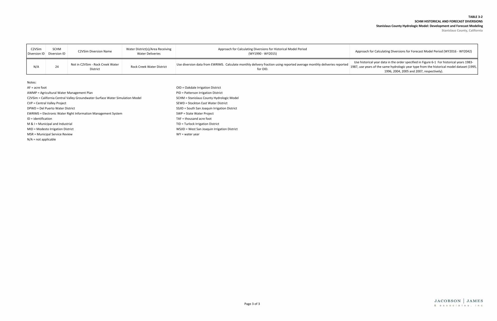
TABLE 3‐2SCHM HISTORICAL AND FORECAST DIVERSIONS
Stanislaus County Hydrologic Model: Development and Forecast ModelingStanislaus County, California
C2VSim Diversion ID
SCHM Diversion ID
C2VSim Diversion NameWater District(s)/Area Receiving
Water DeliveriesApproach for Calculating Diversions for Historical Model Period
(WY1990 ‐ WY2015)Approach for Calculating Diversions for Forecast Model Period (WY2016 ‐ WY2042)
N/A 24Not in C2VSim ‐ Rock Creek Water
DistrictRock Creek Water District
Use diversion data from EWRIMS. Calculate monthly delivery fraction using reported average monthly deliveries reported for OID.
Use historical year data in the order specified in Figure 6‐1 For historical years 1983‐1987, use years of the same hydrologic year type from the historical model dataset (1995,
1996, 2004, 2005 and 2007, respectively).
Notes:AF = acre foot OID = Oakdale Irrigation DistrictAWMP = Agricultural Water Management Plan PID = Patterson Irrigation DistrictC2VSim = California Central Valley Groundwater‐Surface Water Simulation Model SCHM = Stanislaus County Hydrologic ModelCVP = Central Valley Project SEWD = Stockton East Water DistrictDPWD = Del Puerto Water District SSJID = South San Joaquin Irrigation DistrictEWRIMS = Electronic Water Right Information Management System SWP = State Water ProjectID = identification TAF = thousand acre footM & I = Municipal and Industrial TID = Turlock Irrigation DistrictMID = Modesto Irrigation District WSJID = West San Joaquin Irrigation DistrictMSR = Municipal Service Review WY = water yearN/A = not applicable
Page 3 of 3

Stanislaus County Hydrologic Model: Development and Forecasts
Stanislaus County, California
FIGURE 3-1
Water Budget Subregions within SCHM
PROJECT NO.
STANCO.002
DATE
11/10/17
DRAWN BY
JH
APPR. BY
MT
Note: Water budget data for year 2000, based on United States Census information.
Water Budget Subregions General Head Boundary No Flow Boundary Stanislaus County Boundary
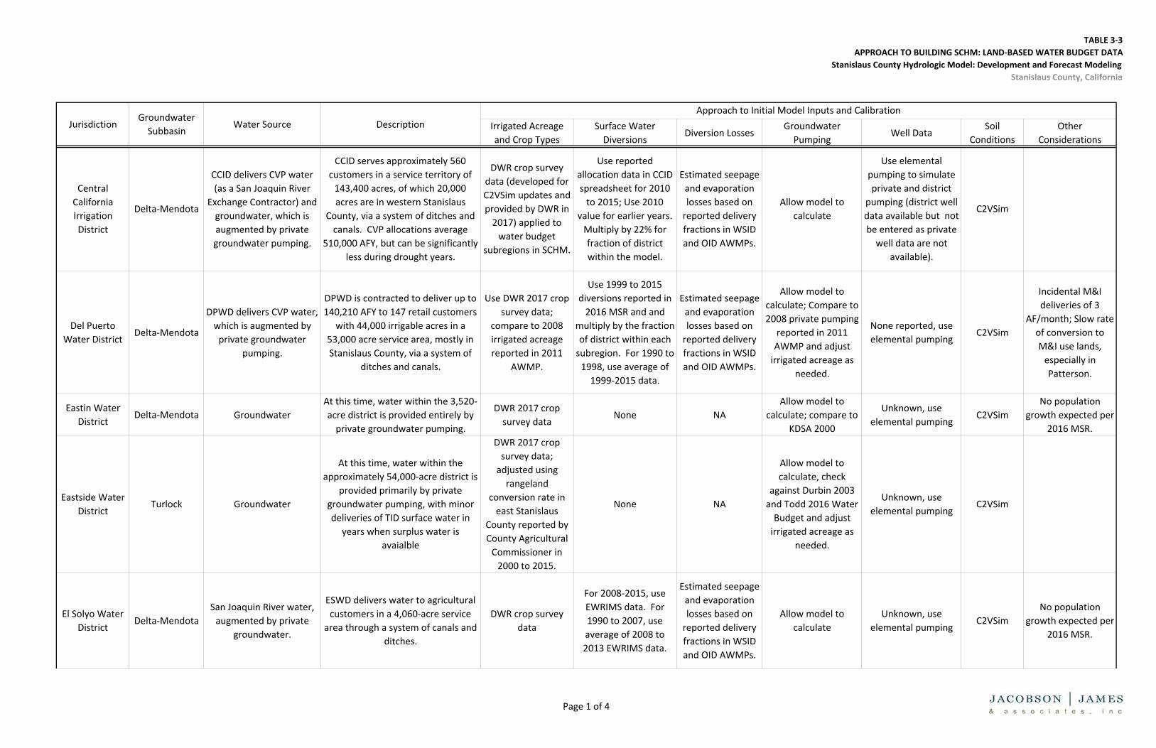
TABLE 3‐3APPROACH TO BUILDING SCHM: LAND‐BASED WATER BUDGET DATA
Stanislaus County Hydrologic Model: Development and Forecast ModelingStanislaus County, California
Irrigated Acreage and Crop Types
Surface Water Diversions
Diversion LossesGroundwater Pumping
Well DataSoil
ConditionsOther
Considerations
Central California Irrigation District
Delta‐Mendota
CCID delivers CVP water (as a San Joaquin River
Exchange Contractor) and groundwater, which is augmented by private groundwater pumping.
CCID serves approximately 560 customers in a service territory of 143,400 acres, of which 20,000 acres are in western Stanislaus
County, via a system of ditches and canals. CVP allocations average
510,000 AFY, but can be significantly less during drought years.
DWR crop survey data (developed for C2VSim updates and provided by DWR in 2017) applied to water budget
subregions in SCHM.
Use reported allocation data in CCID spreadsheet for 2010 to 2015; Use 2010
value for earlier years. Multiply by 22% for fraction of district within the model.
Estimated seepage and evaporation losses based on reported delivery fractions in WSID and OID AWMPs.
Allow model to calculate
Use elemental pumping to simulate private and district
pumping (district well data available but not be entered as private well data are not
available).
C2VSim
Del Puerto Water District
Delta‐Mendota
DPWD delivers CVP water, which is augmented by private groundwater
pumping.
DPWD is contracted to deliver up to 140,210 AFY to 147 retail customers
with 44,000 irrigable acres in a 53,000 acre service area, mostly in Stanislaus County, via a system of
ditches and canals.
Use DWR 2017 crop survey data;
compare to 2008 irrigated acreage reported in 2011
AWMP.
Use 1999 to 2015 diversions reported in 2016 MSR and and
multiply by the fraction of district within each subregion. For 1990 to 1998, use average of 1999‐2015 data.
Estimated seepage and evaporation losses based on reported delivery fractions in WSID and OID AWMPs.
Allow model to calculate; Compare to 2008 private pumping
reported in 2011 AWMP and adjust irrigated acreage as
needed.
None reported, use elemental pumping
C2VSim
Incidental M&I deliveries of 3
AF/month; Slow rate of conversion to M&I use lands, especially in Patterson.
Eastin Water District
Delta‐Mendota GroundwaterAt this time, water within the 3,520‐acre district is provided entirely by private groundwater pumping.
DWR 2017 crop survey data
None NAAllow model to
calculate; compare to KDSA 2000
Unknown, use elemental pumping
C2VSimNo population
growth expected per 2016 MSR.
Eastside Water District
Turlock Groundwater
At this time, water within the approximately 54,000‐acre district is
provided primarily by private groundwater pumping, with minor deliveries of TID surface water in
years when surplus water is avaialble
DWR 2017 crop survey data; adjusted using rangeland
conversion rate in east Stanislaus
County reported by County Agricultural Commissioner in 2000 to 2015.
None NA
Allow model to calculate, check
against Durbin 2003 and Todd 2016 Water Budget and adjust irrigated acreage as
needed.
Unknown, use elemental pumping
C2VSim
El Solyo Water District
Delta‐MendotaSan Joaquin River water, augmented by private
groundwater.
ESWD delivers water to agricultural customers in a 4,060‐acre service
area through a system of canals and ditches.
DWR crop survey data
For 2008‐2015, use EWRIMS data. For 1990 to 2007, use average of 2008 to 2013 EWRIMS data.
Estimated seepage and evaporation losses based on reported delivery fractions in WSID and OID AWMPs.
Allow model to calculate
Unknown, use elemental pumping
C2VSimNo population
growth expected per 2016 MSR.
Approach to Initial Model Inputs and CalibrationJurisdiction
Groundwater Subbasin
Water Source Description
Page 1 of 4

TABLE 3‐3APPROACH TO BUILDING SCHM: LAND‐BASED WATER BUDGET DATA
Stanislaus County Hydrologic Model: Development and Forecast ModelingStanislaus County, California
Irrigated Acreage and Crop Types
Surface Water Diversions
Diversion LossesGroundwater Pumping
Well DataSoil
ConditionsOther
Considerations
Approach to Initial Model Inputs and CalibrationJurisdiction
Groundwater Subbasin
Water Source Description
Modesto Irrigation District
Modesto
Modesto ID delivers Tuolumne River water and groundwater, which is augmented to some extent by private
groundwater pumping.
Modesto ID serves approximately 3,100 retail agricultural irrigation customers on 60,000 acres of
irrigable land in a service territory of approximately 101,700 acres via a system of ditches and canals. In addition, the district delivers
wholesale domestic water to the City of Modesto.
DWR crop survey data; Compare to irrigated acreage and crop water demand in 2015
AWMP.
Calculate based on C2VSim Diversion 100 minus deliveries to City of Modesto; Compare to 2000‐2015 data in summary provided by Modesto ID and 2010‐2014 data in 2015 AWMP. Adjust deliveries to
subregions based on data in USGS, 2004.
Estimated seepage and evaporation losses based on
difference between reported diversions and farm gate
deliveries, adjusted by 20% to account
for possible reporting bias.
Allow model to calculate; compare to data in 2015 AWMP and adjust irrigated acreage as needed.
District well data available, but private well data unknown,
use elemental pumping.
C2VSim
Modesto ID delivers municipal supply to
Modesto; See Modesto UWMP for estimated demand growth over time.
Oak Flat Water District
Delta‐Mendota
OFWD delivers SWP water, which is
augmented by private groundwater pumping.
OFWD is contracted to deliver up to 5,700 AFY to 2,158 irrigable acres in
a 4,537 acre service area via a system of ditches and canals.
DWR crop survey data.
Use reported 2006 ‐ 2015 diversions
reported in 2016 MSR. Calculate 1990‐2005
diversions by multiplying the
maximum allocation by reported SWP delivery
fractions.
Estimated seepage and evaporation losses based on reported delivery fractions in WSID and OID AWMPs.
Allow model to calculate
Unknown, use elemental pumping
C2VSimNo population
growth expected per 2016 MSR.
Oakdale Irrigation District
ModestoEastern San Joaquin
OID delivers Stanislaus River water, drainage
water and groundwater, which is augmented to some extent by private groundwater pumping.
OID serves approximately 2,900 retail agricultural irrigation
customers and nine domestic water systems in a service territory of approximately 73,660 acres via a system of ditches and canals.
DWR crop survey data; Compare to tabulated data for
2009‐2015 in district crop reports
Use data reported in OID‐provided spreadsheet.
Estimated seepage and evaporation losses based on reported delivery
fractions calculated from
OID data.
Allow model to calculate. Compare to data in 2015 AWMP and 2000 to 2015
spreadsheet data and adjust irrigated areage
as needed.
District well data available, but private well data unknown,
use elemental pumping.
C2VSim
Patterson Irrigation District
Delta‐Mendota
PID delivers CVP, reclaimed drainage, groundwater and San Joaquin River Water, which is augmented by private groundwater
pumping.
PID serves approximately 725 retail customsers in a 13,150 acre service area via a system of ditches and
canals.
DWR crop survey data; Compare to irrigated acres and crop water demand reported in 2016
AWMP
Use 2001 to 2010 data from AWMP; For 1990 to 2000 and 2011 to 2013, use the 2001‐2010 average; For 2014 and 2015, use half the average.
Estimated seepage and evaporation losses based on reported delivery fractions in WSID and OID AWMPs.
Allow model to calculate. Compare to groundwater pumping
reported in 2016 AWMP and adjust irrigated areage as
needed.
None reported, use elemental pumping
C2VSim
Growth of the City of Patterson is
expected to result in decreased acreage
served
Page 2 of 4

TABLE 3‐3APPROACH TO BUILDING SCHM: LAND‐BASED WATER BUDGET DATA
Stanislaus County Hydrologic Model: Development and Forecast ModelingStanislaus County, California
Irrigated Acreage and Crop Types
Surface Water Diversions
Diversion LossesGroundwater Pumping
Well DataSoil
ConditionsOther
Considerations
Approach to Initial Model Inputs and CalibrationJurisdiction
Groundwater Subbasin
Water Source Description
Rock Creek Water District
Eastern San Joaquin
RCWD delivers surface water from the Salt Spring Reservoir in Calaveras
County, which is augmented by private groundwater pumping.
RCWD serves four retail customers in a service territory of 1,844 acres
via a canal from Salt Springs Reservoir.
DWR crop survey data
Use EWRIMS data
Estimated seepage and evaporation losses based on reported delivery fractions in WSID and OID AWMPs.
Allow model to calculate.
None reported, use elemental pumping
C2VSimNo population
growth expected
Turlock Irrigation District
Turlock
TID delivers Tuolumne River water and
groundwater, which is augmented to some extent by private
groundwater pumping.
TID serves approximately 5,800 retail agricultural irrigation
customers on 150,000 acres of irrigable land in a service territory of approximately 196,500 acres via system of ditches and canals. In addition, the district delivers
domestic water to the community of La Grange.
DWR crop survey data, compare to crop data provided
by district.
Use Calsim Diversion 107 data after
accounting for losses; Distribute in
accordance with reported subregional farm gate deliveries reported by district.
Use C2VSim data for primary
diversion, adjust using professional judment during calibration
process; Calculate diversion losses for ag deliveries based on TID provided
data.
Allow model to calculate, compare to spreadsheet data provided by district and adjust irrigated acreage and crop water demand as appropriate.
None reported, use elemental pumping
C2VSim, compare to IDC data files provided by district.
West Stanislaus Irrigation District
Delta‐Mendota
WSID delivers water from the San Joaquin River, CVP and groundwater, which is augmented by private groundwater pumping.
WSID serves 83 retail customers in a 21,774 acre service territory via a system of ditches and canals. WSID also sells water to the 2,203 acres in
the White Lake area, north of Grayson.
DWR crop survey data, compare to
district crop data for 2015 and irrigated acreage for 2000‐
2015.
CalSim, allocated proportionally. Compare to
spreadsheet data for 2000 ‐ 2015 and water budgets from 2009 and
2014 AWMPs.
Estimated seepage and evaporation losses based on reported delivery fractions in WSID
AWMP.
Allow model to calculate, compare to spreadsheet data provided by district for 2015, and to 2009 and 2014 AWMPs.
Some district well data available, but private well data unknown, use
elemental pumping.
C2VSim
Growth in Grayson, Westley and Patterson will
decrease irrigated acreage.
Ballico‐Cortez Water District
Turlock Groundwater
At this time, water within the approximately 6,700‐acre district is
provided primarily by private groundwater pumping, with minor deliveries of TID surface water in
years when surplus water is avaialble.
DWR 2017 crop survey data; adjusted using rangeland
conversion rate in east Stanislaus
County reported by County Agricultural Commissioner in 2000 to 2015.
None NA
Allow model to calculate, check
against Durbin 2003 and Todd 2016 Water Budget and adjust irrigated acreage as
appropriate.
Unknown, use elemental pumping
C2VSim
Page 3 of 4

TABLE 3‐3APPROACH TO BUILDING SCHM: LAND‐BASED WATER BUDGET DATA
Stanislaus County Hydrologic Model: Development and Forecast ModelingStanislaus County, California
Irrigated Acreage and Crop Types
Surface Water Diversions
Diversion LossesGroundwater Pumping
Well DataSoil
ConditionsOther
Considerations
Approach to Initial Model Inputs and CalibrationJurisdiction
Groundwater Subbasin
Water Source Description
Merced Irrigation District
Turlock
Merced ID delivers Merced River water and groundwater, which is augmented by private groundwater pumping.
Merced ID delivers up to 310,000 AFY to 2,200 retail customers with 110,000 irrigable acres in a 164,000 acre service area, via a system of ditches and canals. Approximately 10,000 acres of Merced ID's service
territory overlies the Turlock Subbasin in Merced County.
DWR crop survey data, compare to 2016 AWMP
Use 2010 to 2015 data from 2016 AWMP for Northside Canal and Main Canal, and
multiply by the fraction of Merced ID service area for each canal within SCHM. For 1990 to 2009, use C2VSim diversions. Allocate Stevinson Water District deliveries to the corresponding subregions.
Calculate seepage and evaporation losses based on data in the 2016 AWMP and adjust using professional judgment during the calibration
process.
Allow model to calculate, compare to Durbin 2003 Water Budget and 2016 AWMP and adjust
irrigated acreage and crop demand as appropriate
Unknown, use elemental pumping
C2VSim
Notes:AF = acre foot KDSA = Kenneth D. Schmidt and AssociatesAFY = acre foot per year M&I = Municipal and IndustrialAWMP = Agricultural Water Management Plan MSR = Municipal Service ReviewC2VSim = California Central Valley Groundwater Surface Water Simulation Model NA = not availableCalSim = formal name for Water Resource Integrated Modeling System (WRIMS model engine or WRIMS) OFWD = Oak Flat Water DistrictCCID = Central California Irrigation District OID = Oakdale Water DistrictCVP = Central Valley Project RCWD = Rock Creek Water DistrictDPWD = Del Puerto Water District SCHM = Stanislaus County Hydrologic ModelDWR = California Department of Water Resources SWP = State Water ProjectESWD = El Solyo Water District TID = Turlock Irrigation DistrictEWRIMS = Electronic Water Rights Information System USGS = United States Geological SurveyIDC = Irrigation Demand Calculator UWMP = Urban Water Management PlanID = Irrigation District WSID = West Stanislaus Irrigation District
% = percentReferences:Timothy J. Durbin, Inc., 2003. Turlock Groundwater Basin Water Budget 1952 ‐ 2002. Prepared for Turlock Groundwater Basin Association. December. KDSA, 2000. Groundwater Conditions in and near the Eastin Water District. Prepared for Central California Irrigation District and Eastin Water District. February.Todd Groundwater, 2016. Final Report Hydrogeological Characterization of the Eastern Turlock Subbasin. March.USGS, 2004. Hydrogeologic Characterization of the Modesto Area, San Joaquin Valley, California. Scientific Investigations Report 2004‐5232.
Page 4 of 4

TABLE 3‐4SUMMARY OF SCHM DIVERSION LOSS FRACTIONS
Stanislaus County Hydrologic Model: Development and Forecast ModelingStanislaus County, California
C2VSim Diversion ID
SCHM Diversion ID
DescriptionRecoverable Loss Fractiona
Non‐Recoverable Loss Fractionb
Comments
85 1 Calaveras River 0.15 0.32 Calculated from SEWD data
93 2Sacramento‐San Joaquin Delta
to SWP0.1 0.03
Assumed default based on reported typical loss fractions reported in WSID and OID AWMPs and C2VSim
94 3Stanislaus River to South San
Joaquin Canal for Ag0.12 0.06 Calculated from SSJID data
95 4Stanislaus River to South San
Joaquin Canal for M&I0.9 0.1
Professional judgment based on SSJID delivery to recharge basins in Ripon
96 5Stanislaus River to Oakdale
Canal for Agriculture0.1 0.01 Calculated from OID data
98 6Stanislaus River riparian for
Agriculture0.15 0.03
Assumed default based on reported typical loss fractions reported in WSID and OID AWMPs and C2VSim
100 7Tuolumne River to Modesto
Canal0.02 0.01
Adjusted from C2Vsim values during calibration to reflect more reasonable loss factors based on available data
101 8 Modesto Canal for Agriculture 0.15 0.15 Calculated from Modesto Irrigation District data
102 9 Modesto Canal for M&I 0.05 0.01 From C2VSim
103 10Tuolumne River right bank riparian diversions for
Agriculture0.1 0.03
Assumed default based on reported typical loss fractions reported in WSID and OID AWMPs and C2VSim
105 11Tuolumne River left bank riparian diversions for
Agriculture0.1 0.03
Assumed default based on reported typical loss fractions reported in WSID and OID AWMPs and C2VSim
107 12Tuolumne River to Turlock
Canal0.02 0.01
Adjusted from C2Vsim values during calibration to reflect more reasonable loss factors based on available data
108 13 Turlock Canal for Agriculture 0.08 0.05 Calculated from TID data
110 14Merced River to Merced
Irrigation District Northside Canal for Agriculture
0.1 0.22Calculated from Merced Irrigation District data and adjusted during calibration based on professional experience regarding
farm gate delivery reporting
112 15Merced River right bank riparian diversions for
Agriculture0.1 0.03
Assumed default based on reported typical loss fractions reported in WSID and OID AWMPs and C2VSim
114 16Merced River left bank riparian diversions for
Agriculture0.1 0.03
Assumed default based on reported typical loss fractions reported in WSID and OID AWMPs and C2VSim
116 17Merced River to Merced
Irrigation District Main Canal for Agriculture
0.1 0.22Calculated from Merced Irrigation District data and adjusted during calibration based on professional experience regarding
farm gate delivery reporting
128 18
San Joaquin River riparian diversions, Fremont Ford to Vernalis, to Subregion 10 for
Agriculture
0.1 0.03Assumed default based on reported typical loss fractions
reported in WSID and OID AWMPs and C2VSim
129 19
San Joaquin River riparian diversions, Fremont Ford to Vernalis, to Subregion 11 for
Agriculture
0.1 0.03Assumed default based on reported typical loss fractions
reported in WSID and OID AWMPs and C2VSim
130 20
San Joaquin River riparian diversions, Fremont Ford to Vernalis, to Subregion 12 for
Agriculture
0.1 0.03Assumed default based on reported typical loss fractions
reported in WSID and OID AWMPs and C2VSim
Page 1 of 2
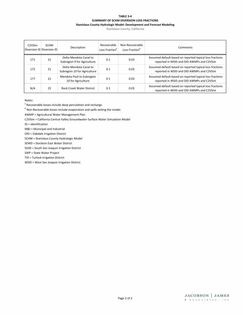
TABLE 3‐4SUMMARY OF SCHM DIVERSION LOSS FRACTIONS
Stanislaus County Hydrologic Model: Development and Forecast ModelingStanislaus County, California
C2VSim Diversion ID
SCHM Diversion ID
DescriptionRecoverable Loss Fractiona
Non‐Recoverable Loss Fractionb
Comments
171 21Delta Mendota Canal to
Subregion 9 for Agriculture0.1 0.03
Assumed default based on reported typical loss fractions reported in WSID and OID AWMPs and C2VSim
172 21Delta Mendota Canal to
Subregion 10 for Agriculture0.1 0.03
Assumed default based on reported typical loss fractions reported in WSID and OID AWMPs and C2VSim
177 21Mendota Pool to Subregion
10 for Agriculture0.1 0.03
Assumed default based on reported typical loss fractions reported in WSID and OID AWMPs and C2VSim
N/A 22 Rock Creek Water District 0.1 0.03Assumed default based on reported typical loss fractions
reported in WSID and OID AWMPs and C2VSim
Notes:a Recoverable losses include deep percolation and recharge.b Non‐Recoverable losses include evaporation and spills exiting the model.AWMP = Agricultural Water Management PlanC2VSim = California Central Valley Groundwater‐Surface Water Simulation ModelID = identificationM&I = Municipal and IndustrialOID = Oakdale Irrigation DistrictSCHM = Stanislaus County Hydrologic ModelSEWD = Stockton East Water DistrictSSJID = South San Joaquin Irrigation DistrictSWP = State Water ProjectTID = Turlock Irrigation DistrictWSID = West San Joaquin Irrigation District
Page 2 of 2
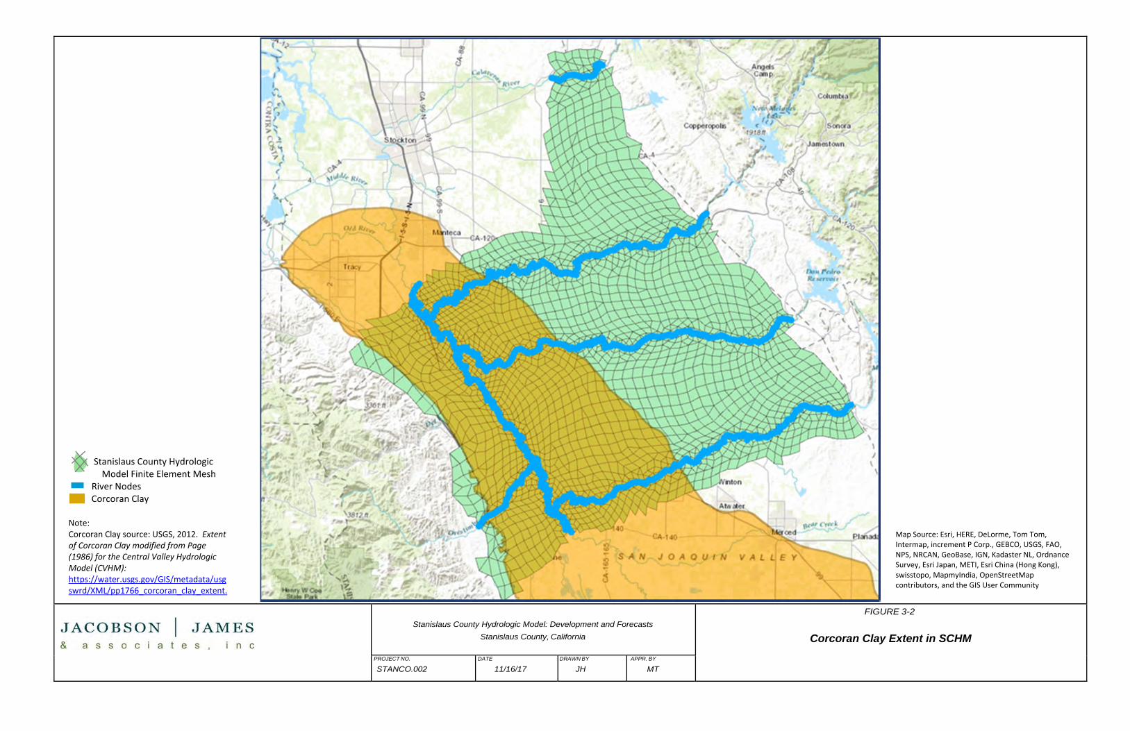
Stanislaus County Hydrologic Model: Development and Forecasts
Stanislaus County, California
FIGURE 3-2
Corcoran Clay Extent in SCHM
PROJECT NO.
STANCO.002
DATE
11/16/17
DRAWN BY
JH
APPR. BY
MT
Stanislaus County Hydrologic Model Finite Element Mesh River Nodes Corcoran Clay Note: Corcoran Clay source: USGS, 2012. Extent of Corcoran Clay modified from Page (1986) for the Central Valley Hydrologic Model (CVHM): https://water.usgs.gov/GIS/metadata/usgswrd/XML/pp1766_corcoran_clay_extent.
Map Source: Esri, HERE, DeLorme, Tom Tom, Intermap, increment P Corp., GEBCO, USGS, FAO, NPS, NRCAN, GeoBase, IGN, Kadaster NL, Ordnance Survey, Esri Japan, METI, Esri China (Hong Kong), swisstopo, MapmyIndia, OpenStreetMap contributors, and the GIS User Community
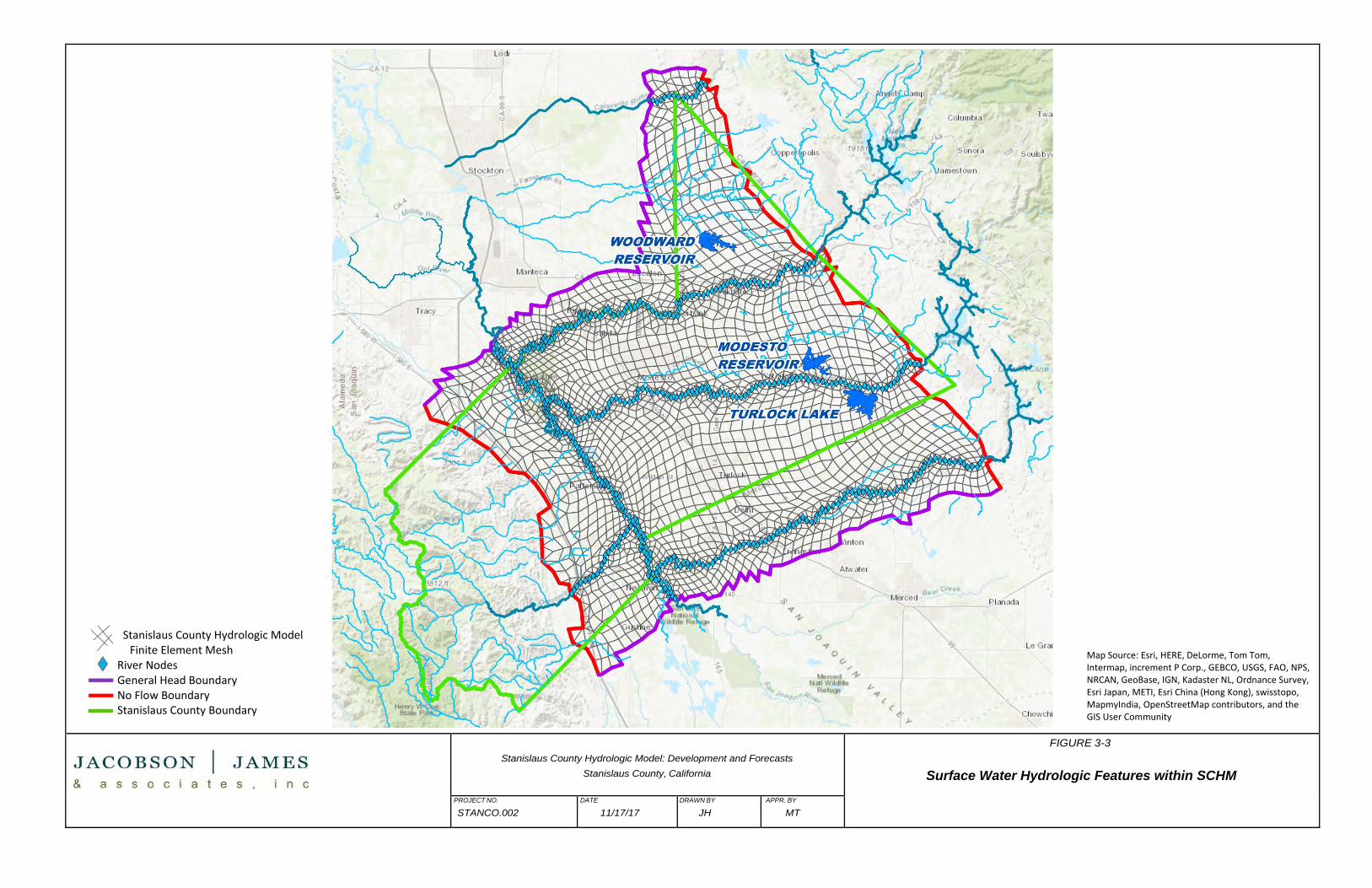
Stanislaus County Hydrologic Model: Development and Forecasts
Stanislaus County, California
FIGURE 3-3
Surface Water Hydrologic Features within SCHM
PROJECT NO.
STANCO.002
DATE
11/17/17
DRAWN BY
JH
APPR. BY
MT
Stanislaus County Hydrologic Model Finite Element Mesh River Nodes General Head Boundary No Flow Boundary Stanislaus County Boundary
Map Source: Esri, HERE, DeLorme, Tom Tom, Intermap, increment P Corp., GEBCO, USGS, FAO, NPS, NRCAN, GeoBase, IGN, Kadaster NL, Ordnance Survey, Esri Japan, METI, Esri China (Hong Kong), swisstopo, MapmyIndia, OpenStreetMap contributors, and the GIS User Community

Stanislaus County Hydrologic Model: Development and Forecasts
Stanislaus County, California
FIGURE 3-4
Location of Municipal Supply Wells and Theoretical Rural Domestic
Supply Wells within SCHM PROJECT NO.
STANCO.002
DATE
11/10/17
DRAWN BY
JH
APPR. BY
MT
Stanislaus County Hydrologic Model Finite Element Mesh General Head Boundary No Flow Boundary Stanislaus County Boundary Theoretical Rural Domestic Supply Wells Municipal Supply Wells

Stanislaus County Hydrologic Model: Development and Forecasts
Stanislaus County, California
FIGURE 3-5
Development of Starting Hydraulic Conductivity for SCHM Layer 1
PROJECT NO.
STANCO.002
DATE
11/17/17
DRAWN BY
JH
APPR. BY
MT
Stanislaus County Hydrologic Model Finite Element Mesh General Head Boundary No Flow Boundary Stanislaus County Boundary MERSTAN (Merced‐Stanislaus) Model Boundary Wells

Stanislaus County Hydrologic Model: Development and Forecasts December 20, 2017
Page 4-1
4.0 CALIBRATION
4.1 Approach
Calibration of model parameters and inputs is an important and necessary step to improve a model’s
reliability to predict future conditions. The amount of effort that is appropriate for calibrating a groundwater
flow model depends on its intended use (USGS, 2004a). In addition, because the response of a groundwater
flow model to introduced stresses is a result of the interaction between a complex series of model inputs and
parameters, a variety of adjustments may result in improved model calibration, but not all of them are
necessarily realistic. Thus, it is possible to improve a model’s calibration response without necessarily making
it better reflect the actual conditions it is intended to simulate. For these reasons, the calibration effort
focused on making manual adjustments to the model inputs and architecture, and it was decided to forego
automated calibration using the Parameter Estimation (PEST) software package, which will not necessarily
result in a unique solution. The following approach was taken to calibrate the SCHM:
• Because the current application of the SCHM is to evaluate the broad programmatic effects of
groundwater well permitting using a superposition approach, the level of calibration judged to be
appropriate is more limited than for a model used to evaluate the more localized effects of specific
projects, or to develop sub-basin scale criteria for sustainable groundwater management as part of a
GSP. Should more detailed application be required in the future, additional data refinement and
calibration could be performed in specific areas of interest.
• Extensive local data have been compiled for construction of the SCHM; however, as discussed in
Section 1.2, substantial uncertainties remain and much additional data are likely available to inform
and refine future modeling efforts. For this reason, calibration efforts were focused on making
changes that were consistent with our understanding of the model hydrogeology and water budget,
and on documenting the remaining opportunities for additional refinement and calibration in the
future. Calibration activities therefore focused on the following tasks:
o Adjustments to the model water budget were made when comparison between the model
water budget and data provided by local districts or available in water management plans
indicated a discrepancy that needed correction.
o Adjustments to model boundary conditions were implemented where significant
discrepancies were observed between boundary heads extracted from C2VSim and near-
boundary calibration wells.
o Adjustments to aquifer parameters (lateral and vertical hydraulic conductivity) were made
in an iterative fashion in areas where a bias in calibration results was observed, and where
those adjustments were consistent with specific conceptual model refinements, i.e., where
there was a specific hydrogeologic rationale for making the changes.

Stanislaus County Hydrologic Model: Development and Forecasts December 20, 2017
Page 4-2
o Adjustments to streambed conductance and recharge distribution from small watersheds
were made where surface water flow and groundwater level data indicated a discrepancy
that could be related to surface/groundwater interaction.
4.2 Calibration Datasets
The following dataset of calibration wells and gaging stations was assembled to support the
calibration process. Locations of these calibration points are shown on Figure 4-1.
• Sixty-three (63) calibration wells designed in C2VSim within the SCHM model domain were adopted
as calibration wells for the model. Groundwater elevation data for these wells after WY 2009 (the
current cutoff date in C2VSim) were obtained from the CASGEM database to complete the calibration
dataset for these wells.
• One hundred one (101) additional calibration wells were selected from the CASGEM database for use
in portions of the SCHM domain that were under-represented in the C2VSim calibration dataset.
• Seven gaging stations were selected from the USGS National Water Information System (NWIS) to
represent inflows and outflows from the model along the major streams.
Each calibration well was evaluated for data quality and assigned to a particular model layer or layers. In a
limited number of cases, data labeled as questionable by CASGEM were removed when individual data points
appeared to be anomalous, but in most cases, all of the water level data were retained. At each well,
predicted water levels in Model Layers 1 and 2 were compared to measured water levels, and the results
were evaluated in relation to well depth and screen interval (when reported) and to data from nearby wells.
In a number of cases, it was found that wells that penetrated to a completion depth within the deeper aquifer
system (Layer 2) nevertheless displayed water levels that were more representative of the shallow aquifer
system (Layer 1). This was especially the case in areas where groundwater levels in the upper aquifer system
are significantly higher than in the deeper aquifer system, suggesting that the well screens or gravel packs are
cross connecting the two aquifer systems and the hydraulic signal from the upper aquifer is dominating
groundwater levels in the well. In such cases, the wells were assigned to Layer 1. Thirteen calibration (13)
calibration wells were considered representative of groundwater levels in both Layers 1 and 2, and are
designated and compared as separate wells in the calibration well data set.
4.3 Model Adjustments
4.3.1 Water Budget Adjustments
Because the water budget data compiled for development of the SCHM were considered the most reliable
data for characterization of local conditions, the first step of model calibration consisted of comparing model
water budget data to the compiled dataset, making adjustments where appropriate, and evaluating the effect
of these changes on the groundwater level and surface water flow calibration results. Information regarding
municipal surface water deliveries and groundwater pumping was considered reliable as entered into the

Stanislaus County Hydrologic Model: Development and Forecasts December 20, 2017
Page 4-3
model using the procedure summarized in Table 3-1, so efforts were focused primarily on refinement and
calibration of the agricultural water budget using the procedure summarized in Table 3-3. These initial
calibration steps were conducted as described below, and resulted in a substantial improvement in model
conformance with historical calibration well groundwater levels and trends.
4.3.1.1 Water Diversions and Deliveries
Surface water deliveries ascribed in the SCHM to each of the 17 water and irrigation and districts shown on
Figure 2-1 were compared to data obtained from the districts or compiled from AWMPs, MSRs and other
plans and reports as outlined in Table 3-3. This process was conducted iteratively, and effects on model
calibration were evaluated at each step. Where discrepancies were noted, the diversions were adjusted,
redistributed between the assigned water budget subareas, and/or the loss factors for the diversions were
adjusted such that farm gate deliveries more closely approximated reported values. Consistent with the
approach taken by the USGS to recent updates of the MERSTAN model, loss factors for some districts were
adjusted downward when warranted by calibration data in order to compensate for the potential
underestimation of deliveries.8 For Modesto Irrigation District, water deliveries were allocated throughout
the district’s service areas in proportion to the delivery fractions reported in the USGS documentation for the
MERSTAN model (USGS, 2004b). For TID, water deliveries were allocated throughout the district’s service
areas based on data provided by the district. The TID dataset was considered the most extensive and reliable
provided, and after this initial calibration step, surface water deliveries in the SCHM were approximately 98%
of reported farm gate deliveries. The final diversion and diversion loss values adopted in the SCHM are
summarized in Tables 3-2 and 3-4, respectively.
4.3.1.2 Land Use-Based Water Budget Data
The second step in the calibration process consisted of comparing the groundwater pumping calculated by
the model in each water and irrigation district to reported pumping data obtained from the districts or
compiled from AWMPs, MSRs and other plans and reports as outlined in Table 3-3. This process was
conducted iteratively, and effects on model calibration were evaluated at each step. Where discrepancies
were noted, the irrigated acreage and in some cases crop types were adjusted to align the pumping more
closely with the reported values. The most extensive changes during this step were made in the eastern,
foothill portion of the model, and changes were made in consideration of aerial imagery that confirmed
changes in cropping patterns, and a geospatial analysis cropping trends in eastern, non-district lands provided
by the Stanislaus County Agricultural Commissioner (Appendix A).
4.3.1.3 Initial and Boundary Heads
After implementation of refinements to the diversions and cropping were made, the assigned heads for the
time-dependent head boundaries were adjusted to match nearby historical data as needed so as to minimize
potential boundary effects. This was accomplished by examining data for calibration wells located near the
8 Per personal communication from Stephen Phillips, USGS, in November 2017 with Walter Ward.

Stanislaus County Hydrologic Model: Development and Forecasts December 20, 2017
Page 4-4
SCHM northern and southern general head boundaries, and interpolating boundary node head elevations
based on nearby spatial and temporal water level data. The resulting adjusted boundary heads were loaded
into the model files.
4.3.2 Reservoirs and Small Watersheds
After the initial calibration steps, it was found that predicted groundwater levels near and downgradient of
Turlock Lake were consistently higher than calibration well groundwater levels. Since the calculated leakage
from Turlock Lake was significantly higher than leakage rates reported and calculated for Woodward and
Modesto Reservoirs, it was decided to decrease the recoverable losses from Turlock Lake from 100% to 33%.
This change improved the calibration for wells in this region.
Recharge from small watersheds was adjusted in areas where, based on calibration results, the known
hydrology and hydrogeology of the area, and professional judgment, recharge had either been over or
underestimated. This primarily consisted of increasing recharge in proximal alluvial fan areas along the Diablo
range near the western no-flow boundary of the model, and in the northern triangle area of the County,
where local investigations have indicated that recharge from small streams is more prominent than was
reflected in the existing version of C2VSim (JJ&A, 2016a and 2017a). In addition, recharge from small streams
along the southeastern no-flow boundary of the model appeared to be overestimated when compared to
similar areas further north. In order to adjust recharge form small watersheds, recharge nodes within the
model domain were added or moved as deemed appropriate based on local scale geology, and the maximum
recharge assigned to the nodes was altered (increased or decreased, as appropriate). This process was
conducted iteratively, and effects on model calibration were evaluated at each step.
4.3.3 Streambed Conductance
Next, stream discharge predicted by the model at river nodes corresponding to the calibration gaging stations
was compared to actual gaging station data. Adjustments were made to the hydraulic conductivity term of
the streambed conductance in groundwater-connected reaches upstream of gaging stations where a bias
was observed between actual and predicted data. This process was conducted iteratively, and the effects on
model calibration were evaluated at each step.
4.3.4 Aquifer Hydraulic Conductivity
As a final calibration step, targeted manual changes were made to the model hydraulic conductivity of Layers
1 and/or 2. These changes were implemented in areas where a bias was noted in the model to either under-
or over-predict groundwater levels, and a rational hydrogeologic explanation could be made to justify the
adjustment that did not contradict the findings of prior studies. Within the portion of the SCHM where
hydraulic conductivities were extracted from the MERSTAN model (which were based on extensive and
detailed geostatistical evaluation of aquifer textural data), care was taken to target changes to follow areas
where the prior analysis could have produced a bias (such as through end-point scaling of permeability) and
not to randomly make changes simply based on calibration results. Changes were broadly applied to aquifer

Stanislaus County Hydrologic Model: Development and Forecasts December 20, 2017
Page 4-5
vertical hydraulic conductivity, which was more poorly constrained by data. Outside the area of the MERSTAN
model, changes to the initial model hydraulic conductivity were more liberally applied based on calibration
data, with care being taken that they follow the local hydrogeologic conceptual understanding and match
conditions in the adjacent MERSTAN area. This process was conducted iteratively, and effects on model
calibration were evaluated at each step. It was clearly evident that the effect of hydraulic conductivity on
model performance was both locally and regionally complex, and that multiple adjustments could result in
“improved” model calibration, without necessarily being a better representation of actual aquifer conditions.
It was therefore decided that less focus would be based on parameter adjustment than on water budget
adjustment during the calibration process. For this reason, calibration was continued only until the objectives
for use of the model for programmatic impact assessment under the PEIR were met. Automated calibration
using PEST was not performed, and iterative parameter calibration was limited pending the collection of
additional data by workers involved in GSP development that would help to guide the direction of further
calibration.
4.3.5 Aquitard Vertical Hydraulic Conductivity
The vertical permeability of the regional Corcoran Clay aquitard and its local variation are poorly understood
in the SCHM area and has a profound effect on local groundwater flow patterns. Permeability can vary locally
and can be changed by artificial penetrations such as composite wells, absence of well seals, damaged wells,
or cross connections created by unsealed boreholes. Adjustments were made to the Corcoran Clay vertical
permeability where calibration data indicated that either more or less vertical flow across this aquitard may
be locally occurring than represented by the assumed uniform hydraulic conductivity in the SCHM. This
process was conducted iteratively, and effects on model calibration were evaluated at each step. Similar to
aquifer hydraulic conductivity, it was evident that the effect of aquitard hydraulic conductivity on model
performance was both locally and regionally complex, that multiple combinations of adjustments could result
in the same “improvements” in model calibration. Adjustment of this parameter was therefore focused on
the objective of using the model as a programmatic impact assessment tool for the PEIR.
4.4 Calibration Results
4.4.1 Groundwater Level Calibration Results
Figures 4-2 and 4-3 show plots of the measured vs. the predicted water levels and the residual vs. the
measured water levels in each calibration well, respectively. The plots on Figure 4-2 clearly show a clustering
of results near the 1:1 correlation line, indicating that at many times and locations the model results are well
aligned with historical results. Overall, more points tend to fall below the lines, indicating a slight overall bias
of the model to under-predict heads. The clustering of points in bands reflects a bias to either over or under-
predict that is associated with particular areas in the model. The biases in these areas could likely be corrected
through additional investigation into local conditions and refinement of the model. At some calibration wells,
the model under or overpredicts actual heads by several tens of feet. Calibration statistics for the final
calibrated model are summarized in Table 4-1, below.
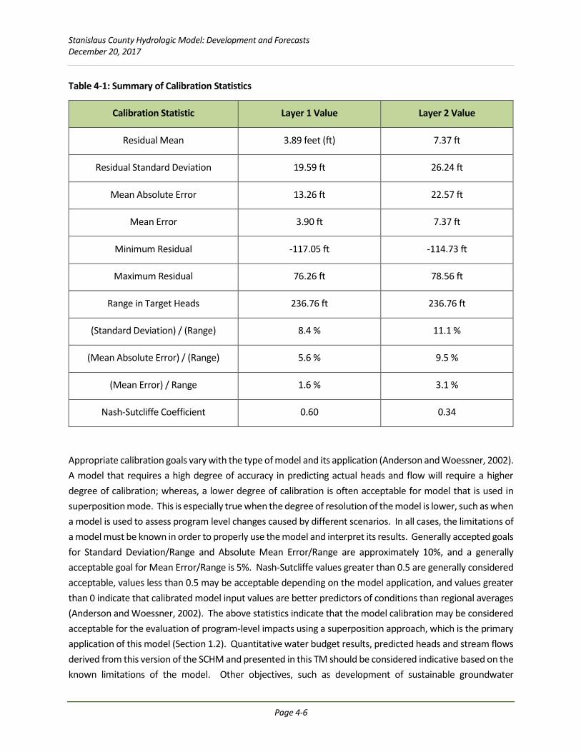
Stanislaus County Hydrologic Model: Development and Forecasts December 20, 2017
Page 4-6
Table 4-1: Summary of Calibration Statistics
Calibration Statistic Layer 1 Value Layer 2 Value
Residual Mean 3.89 feet (ft) 7.37 ft
Residual Standard Deviation 19.59 ft 26.24 ft
Mean Absolute Error 13.26 ft 22.57 ft
Mean Error 3.90 ft 7.37 ft
Minimum Residual -117.05 ft -114.73 ft
Maximum Residual 76.26 ft 78.56 ft
Range in Target Heads 236.76 ft 236.76 ft
(Standard Deviation) / (Range) 8.4 % 11.1 %
(Mean Absolute Error) / (Range) 5.6 % 9.5 %
(Mean Error) / Range 1.6 % 3.1 %
Nash-Sutcliffe Coefficient 0.60 0.34
Appropriate calibration goals vary with the type of model and its application (Anderson and Woessner, 2002).
A model that requires a high degree of accuracy in predicting actual heads and flow will require a higher
degree of calibration; whereas, a lower degree of calibration is often acceptable for model that is used in
superposition mode. This is especially true when the degree of resolution of the model is lower, such as when
a model is used to assess program level changes caused by different scenarios. In all cases, the limitations of
a model must be known in order to properly use the model and interpret its results. Generally accepted goals
for Standard Deviation/Range and Absolute Mean Error/Range are approximately 10%, and a generally
acceptable goal for Mean Error/Range is 5%. Nash-Sutcliffe values greater than 0.5 are generally considered
acceptable, values less than 0.5 may be acceptable depending on the model application, and values greater
than 0 indicate that calibrated model input values are better predictors of conditions than regional averages
(Anderson and Woessner, 2002). The above statistics indicate that the model calibration may be considered
acceptable for the evaluation of program-level impacts using a superposition approach, which is the primary
application of this model (Section 1.2). Quantitative water budget results, predicted heads and stream flows
derived from this version of the SCHM and presented in this TM should be considered indicative based on the
known limitations of the model. Other objectives, such as development of sustainable groundwater
Stanislaus County Hydrologic Model: Development and Forecasts December 20, 2017
Page 4-7
management criteria, or evaluating the effects of specific projects, may require a greater degree of model
refinement and calibration, and potentially a more refined model grid. Such refinements could be targeted
at the model subareas where more rigorous data are needed.
4.4.2 Stream Discharge Calibration Results
A comparison of predicted stream discharge and corresponding measurements at the seven selected
calibration gaging stations (Table 4-2) is provided in Figures 4-4 and 4-5. As shown in the figure, the predicted
and observed stream flows at the gaging stations are closely correlated, with the following exceptions:
• Discharge on the Tuolumne River at the Modesto gaging station is somewhat overpredicted by the
model during low flow periods, indicating that groundwater discharge to the river may also be
overpredicted.
• At the gaging station on Orestimba Creek, which is located near its confluence with the San Joaquin
River, the model significantly under-predicts flow. This is due to the fact that in this area model heads
in Layer 1 are under-predicted relative to measured groundwater levels at nearby calibration wells,
and as a result the stream is modeled as being disconnected from the groundwater table. Data from
nearby calibration wells suggests that in fact Orestimba Creek is groundwater connected and gaining
in its middle and lower reaches. This was accepted as a model limitation that should be addressed
during future modeling efforts when additional data are available or evaluations conducted to select
the appropriate approach to improving the calibration.
4.5 Calibrated Historical Model Results
4.5.1 Hydraulic Conductivity
The final lateral hydraulic conductivity distribution for Model Layers 1, 2, and 3 is shown in Figure 4-6.
The model retains many of the characteristics of the original hydraulic conductivity distribution extracted
from the MERSTAN with local adjustments, and more significant refinements to the original C2VSim hydraulic
conductivity outside the MERSTAN model domain boundaries and west of the San Joaquin River. In general,
areas of higher hydraulic conductivity are concentrated in Layer 1 near the current river corridors.
4.5.2 Groundwater Levels and Flow
Simulated groundwater level elevations for Model Layers 1 and 2 are shown for 2000 and 2015 in
Figure 4-7 and Figure 4-8, respectively. Groundwater levels and flow directions are generally consistent with
historical maps available from DWR through the Groundwater Information Center Interactive Mapping
Application (DWR, 2017b). In general, groundwater flows away from the Sierra Nevada and the Diablo Range
toward the San Joaquin River, and then northward along the valley axis. A prominent cone of depression is
evident in the eastern Turlock Subbasin. Contours near the major streams in the Study area suggest both
gaining and losing reaches where prior studies have generally determined they should be located (USGS,
2004b and 2015).

Stanislaus County Hydrologic Model: Development and Forecasts December 20, 2017
Page 4-8
4.5.3 Groundwater Budget
The final, calibrated model diversions are summarized in Tables 3-2 and 3-4, and the water budget for WY
2000, 2005, 2010 and 2015, broken down by subbasin, is summarized in Table 4-3. As noted above, these
water budget data should be considered indicative and preliminary; however, the following key observations
may be made:
• Both increases and decreases in simulated groundwater storage were observed in the Study Area
during the historical evaluation period of the model (WY 2000 to WY 2015). Simulated storage
changes are related to variations in hydrologic conditions, the amount of surface water available for
irrigation, and the amount of groundwater pumping. As expected, the greatest storage depletions
were observed in 2015, at the height of the recent drought.
• Simulated groundwater recharge from streams has generally increased (groundwater discharge to
streams has decreased) in the Modesto and Turlock Subbasins. This is consistent with data
summarized in Table 4-4, which indicates that simulated groundwater discharge to the Merced,
Stanislaus and Tuolumne Rivers is decreasing over time.
• There is a decrease in simulated deep percolation over time across the Study Area.
• A decrease in simulated net underflow into the Turlock Subbasin is evident over time, as discussed in
greater detail in Section 4.5.4, below.
• There is an increase in simulated net underflow over time out of the portion of the Eastern San
Joaquin Subbasin that lies within the SCHM. A portion of this increase may be related to flow
southward into the Modesto Subbasin, as discussed in greater detail in Section 4.5.4, below, but a
portion may also be associated with underflow across the county boundary to the west out of the
Study Area.
• Simulated agricultural pumping accounts for 80 to 89% of groundwater extraction in the Study Area,
and has been variable and dependent on the amount of surface water available for irrigation. The
highest agricultural pumping rates were observed at the height of the recent drought during WY
2015. No clear trends are evident, except in the Eastern San Joaquin Subbasin, where a steady
increase in agricultural pumping is evident. This trend is consistent with conversion of rangeland to
irrigated agriculture in the eastern foothill area of the model during this time period.
• Simulated municipal pumping accounts for 9 to 18% of groundwater extraction in the Study Area,
with more limited variability in actual pumping rates than agricultural pumping rates (approximately
90,000 to 110,000 AFY). Pumping rates were generally lowest in 2015, likely due to the effect of
water conservation measures that were implemented during the drought.
• Simulated rural domestic pumping accounts for just 1 to 2% of total groundwater extraction in the
Study Area, and was modeled to increase with increasing rural population over time.

Stanislaus County Hydrologic Model: Development and Forecasts December 20, 2017
Page 4-9
4.5.4 Interbasin Flows
Interbasin flows simulated between the subbasins that underlie the SCHM domain in WY 2000, 2005, 2010
and 2015 are summarized in Table 4-5. As noted above, these water budget data should be considered
indicative and preliminary; however, the following key observations may be made:
• Turlock Subbasin. Underflow into the Turlock Subbasin occurs from the Merced Subbasin to the
south and the Modesto Subbasin to the north. Simulated underflow from the Merced Subbasin
decreases over time, and the net direction of simulated underflow in Layer 1 reverses direction from
northward to southward between WY 2010 and WY 2015. Simulated underflow southward into the
Turlock Subbasin from the Modesto Subbasin is variable and does not display a distinct trend,
although the rate is greatest in WY 2015, at the height of the recent drought. Simulated underflow
out of the Turlock Subbasin is less than underflow in, occurs to the Delta-Mendota Subbasin to the
west, and displays a generally increasing trend over time.
• Modesto Subbasin. Underflow into the Modesto Subbasin occurs from the Eastern San Joaquin
Subbasin to the north. Simulated underflow from the Eastern San Joaquin Subbasin decreases over
time in Layer 1, but does not display a distinct trend in Layer 2. Simulated underflow out of the
Modesto Subbasin is greater than underflow in, and occurs to the Turlock Subbasin to the south and
the Delta-Mendota Subbasin to the west. Distinct trends in the rate of underflow out of the subbasin
are not evident, but the greatest rate of underflow out was simulated in WY 2015, at the height of
the recent drought.
• Delta-Mendota Subbasin. Underflow into the portion of the Delta-Mendota Subbasin in the Study
Area is simulated to occur in Layer 1 primarily from the Modesto and Turlock Subasins to the east. In
Layer 2, underflow into the subbasin is simulated to occur primarily from the Modesto and Turlock
Subbasins to the east, and the Tracy Subbasin to the north. It should be noted that there are few
calibration wells in the SCHM in the northern portion of the Delta-Mendota Subbasin, so that
groundwater levels and flow directions in the confined aquifer system in this area may need further
confirmation and the model may require refinement before drawing conclusions regarding cross
boundary flows between the Delta-Mendota and Tracy Subbasins. Simulated underflow into the
Delta-Mendota Subbasin from the Turlock and Modesto Subbasins displays a generally increasing
trend over time. The SCHM does not simulate any significant outflow from the Delta-Mendota
Subbasin.
• Eastern San Joaquin Subbasin. The SCHM does not simulate any significant underflow into the
portion of the Eastern San Joaquin Subbasin in the Study Area. Underflow out of the portion of the
Eastern San Joaquin Subbasin in the Study Area is simulated to occur primarily into the Modesto
Subbasin to the south. The simulated rate of underflow out is variable, but generally increasing over
time.
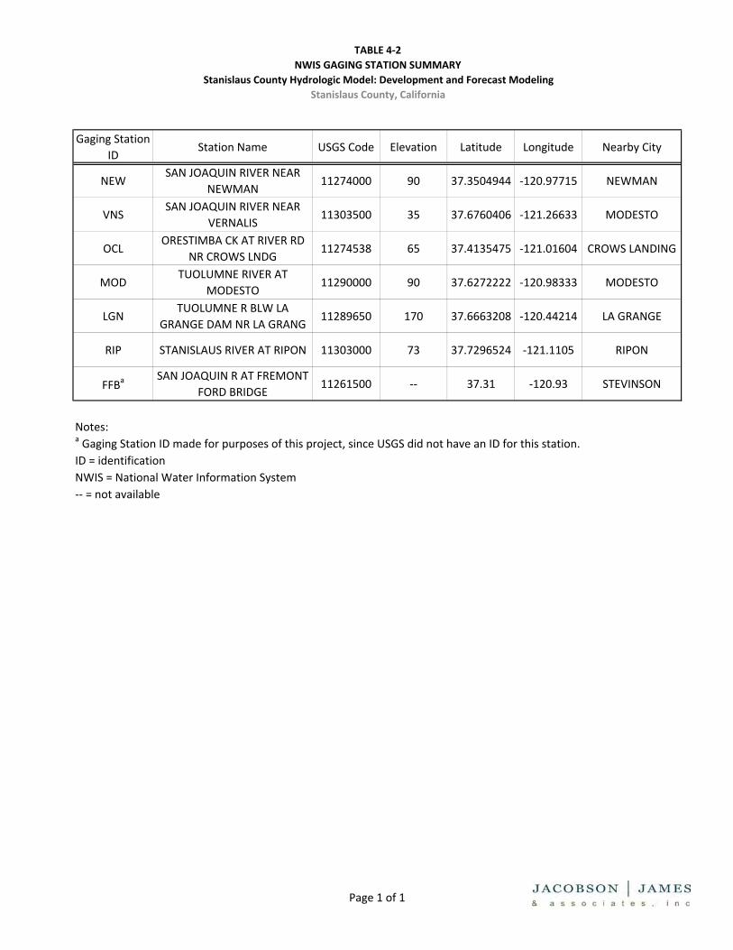
TABLE 4‐2NWIS GAGING STATION SUMMARY
Stanislaus County Hydrologic Model: Development and Forecast ModelingStanislaus County, California
Gaging Station ID
Station Name USGS Code Elevation Latitude Longitude Nearby City
NEWSAN JOAQUIN RIVER NEAR
NEWMAN11274000 90 37.3504944 ‐120.97715 NEWMAN
VNSSAN JOAQUIN RIVER NEAR
VERNALIS11303500 35 37.6760406 ‐121.26633 MODESTO
OCLORESTIMBA CK AT RIVER RD
NR CROWS LNDG11274538 65 37.4135475 ‐121.01604 CROWS LANDING
MODTUOLUMNE RIVER AT
MODESTO11290000 90 37.6272222 ‐120.98333 MODESTO
LGNTUOLUMNE R BLW LA
GRANGE DAM NR LA GRANG11289650 170 37.6663208 ‐120.44214 LA GRANGE
RIP STANISLAUS RIVER AT RIPON 11303000 73 37.7296524 ‐121.1105 RIPON
FFBaSAN JOAQUIN R AT FREMONT
FORD BRIDGE11261500 ‐‐ 37.31 ‐120.93 STEVINSON
Notes:a Gaging Station ID made for purposes of this project, since USGS did not have an ID for this station.ID = identificationNWIS = National Water Information System‐‐ = not available
Page 1 of 1
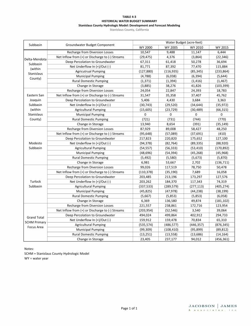
TABLE 4-3
HISTORICAL WATER BUDGET SUMMARY
Stanislaus County Hydrologic Model: Development and Forecast Modeling
Stanislaus County, California
WY 2000 WY 2005 WY 2010 WY 2015
Recharge from Diversion Losses 10,547 9,488 11,147 6,444
Net Inflow from (+) or Discharge to (-) Streams (29,475) 4,376 (3,864) (22,346)
Deep Percolation to Groundwater 67,311 61,418 50,278 36,694
Net Underflow In (+)/Out (-) 81,771 87,392 77,470 115,884
Agricutrual Pumping (127,880) (116,935) (85,345) (233,864)
Municipal Pumping (4,788) (6,038) (6,394) (5,644)
Rural Domestic Pumping (1,371) (1,394) (1,416) (1,467)
Change in Storage (3,885) 38,276 41,826 (103,399)
Recharge from Diversion Losses 24,054 22,847 24,393 18,783
Net Inflow from (+) or Discharge to (-) Streams 31,547 35,358 37,407 45,762
Deep Percolation to Groundwater 5,406 4,430 3,684 3,363
Net Underflow In (+)/Out (-) (30,743) (29,520) (34,644) (35,972)
Agricultural Pumping (15,605) (23,729) (30,489) (66,315)
Municipal Pumping 0 0 0 0
Rural Domestic Pumping (721) (731) (744) (770)
Change in Storage 13,940 8,654 (391) (35,149)
Recharge from Diversion Losses 87,929 89,008 58,427 48,250
Net Inflow from (+) or Discharge to (-) Streams (95,648) (57,089) (37,691) (410)
Deep Percolation to Groundwater 217,823 220,820 175,652 127,100
Net Underflow In (+)/Out (-) (94,378) (82,764) (89,335) (88,920)
Agricultural Pumping (54,557) (56,333) (53,410) (170,892)
Municipal Pumping (48,696) (54,394) (45,268) (45,968)
Rural Domestic Pumping (5,492) (5,580) (5,673) (5,870)
Change in Storage 6,981 53,667 2,702 (136,711)
Recharge from Diversion Losses 99,026 117,519 78,750 50,478
Net Inflow from (+) or Discharge to (-) Streams (110,378) (35,190) 7,689 16,058
Deep Percolation to Groundwater 203,485 213,196 173,297 127,576
Net Underflow In (+)/Out (-) 203,262 184,370 117,343 74,319
Agricultural Pumping (337,533) (289,579) (277,113) (405,274)
Municipal Pumping (45,825) (47,978) (44,238) (38,199)
Rural Domestic Pumping (5,667) (5,853) (5,853) (6,058)
Change in Storage 6,369 136,580 49,874 (181,102)
Recharge from Diversion Losses 221,557 238,861 172,716 123,954
Net Inflow from (+) or Discharge to (-) Streams (203,954) (52,546) 3,540 39,064
Deep Percolation to Groundwater 494,024 499,864 402,912 294,733
Net Underflow In (+)/Out (-) 159,912 159,478 70,834 65,310
Agricultural Pumping (535,574) (486,577) (446,357) (876,345)
Municipal Pumping (99,309) (108,410) (95,899) (89,812)
Rural Domestic Pumping (13,251) (13,558) (13,686) (14,164)
Change in Storage 23,405 237,177 94,012 (456,361)
Notes:
SCHM = Stanislaus County Hydrologic Model
WY = water year
Grand Total
SCHM Primary
Focus Area
Water Budget (acre-feet)
Delta-Mendota
Subbasin
(within
Stanislaus
County)
Eastern San
Joaquin
Subbasin
(within
Stanislaus
County)
Modesto
Subbasin
Turlock
Subbasin
Groundwater Budget ComponentSubbasin
Page 1 of 1

TABLE 4-4
HISTORICAL STREAMFLOW GAIN/LOSS
Stanislaus County Hydrologic Model: Development and Forecast Modeling
Stanislaus County, California
WY 2000 WY 2005 WY 2010 WY 2015
Merced River 10,929 (49,573) (117,162) (122,373)
Orestimba Creek 2 (10,477) (20,986) (18,053) (5,827)
San Joaquin River 79,513 33,288 43,864 60,340
Stanislaus River (2,820) (9,329) (35,801) (85,214)
Tuolumne River 156,597 101,418 76,181 40,841
Notes:
WY = water year
Gain/Loss from Groundwater (acre-feet/year) 1
Stream Reach
1 Based on the level of model calibration, streamflow gain/loss values should be
considered indicative.2 Hydrograph calibration for Orestimba Creek is relatively poor; therefore the results
for this stream should not be considered indicative.
Page 1 of 1
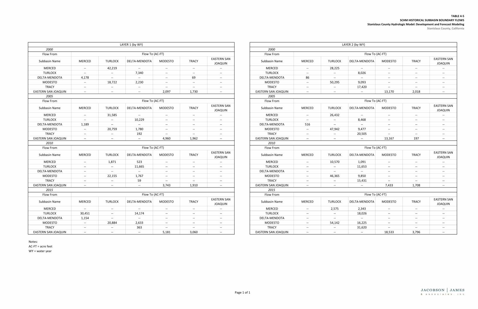
TABLE 4‐5SCHM HISTORICAL SUBBASIN BOUNDARY FLOWS
Stanislaus County Hydrologic Model: Development and Forecast ModelingStanislaus County, California
2000 2000Flow From Flow From
Subbasin Name MERCED TURLOCK DELTA‐MENDOTA MODESTO TRACYEASTERN SAN JOAQUIN
Subbasin Name MERCED TURLOCK DELTA‐MENDOTA MODESTO TRACYEASTERN SAN JOAQUIN
MERCED ‐‐ 42,219 ‐‐ ‐‐ ‐‐ ‐‐ MERCED ‐‐ 28,225 ‐‐ ‐‐ ‐‐ ‐‐TURLOCK ‐‐ ‐‐ 7,340 ‐‐ ‐‐ ‐‐ TURLOCK ‐‐ ‐‐ 8,026 ‐‐ ‐‐ ‐‐
DELTA‐MENDOTA 4,178 ‐‐ ‐‐ ‐‐ 69 ‐‐ DELTA‐MENDOTA 86 ‐‐ ‐‐ ‐‐ ‐‐ ‐‐MODESTO ‐‐ 18,722 2,230 ‐‐ ‐‐ ‐‐ MODESTO ‐‐ 50,295 9,093 ‐‐ ‐‐ ‐‐TRACY ‐‐ ‐‐ ‐‐ ‐‐ ‐‐ ‐‐ TRACY ‐‐ ‐‐ 17,420 ‐‐ ‐‐ ‐‐
EASTERN SAN JOAQUIN ‐‐ ‐‐ ‐‐ 2,097 1,730 ‐‐ EASTERN SAN JOAQUIN ‐‐ ‐‐ ‐‐ 13,170 2,018 ‐‐2005 2005
Flow From Flow From
Subbasin Name MERCED TURLOCK DELTA‐MENDOTA MODESTO TRACYEASTERN SAN JOAQUIN
Subbasin Name MERCED TURLOCK DELTA‐MENDOTA MODESTO TRACYEASTERN SAN JOAQUIN
MERCED ‐‐ 31,585 ‐‐ ‐‐ ‐‐ ‐‐ MERCED ‐‐ 26,432 ‐‐ ‐‐ ‐‐ ‐‐TURLOCK ‐‐ ‐‐ 10,229 ‐‐ ‐‐ ‐‐ TURLOCK ‐‐ ‐‐ 8,468 ‐‐ ‐‐ ‐‐
DELTA‐MENDOTA 1,189 ‐‐ ‐‐ ‐‐ ‐‐ ‐‐ DELTA‐MENDOTA 516 ‐‐ ‐‐ ‐‐ ‐‐ ‐‐MODESTO ‐‐ 20,759 1,780 ‐‐ ‐‐ ‐‐ MODESTO ‐‐ 47,942 9,477 ‐‐ ‐‐ ‐‐TRACY ‐‐ ‐‐ 192 ‐‐ ‐‐ ‐‐ TRACY ‐‐ ‐‐ 20,505 ‐‐ ‐‐ ‐‐
EASTERN SAN JOAQUIN ‐‐ ‐‐ ‐‐ 4,960 1,962 ‐‐ EASTERN SAN JOAQUIN ‐‐ ‐‐ ‐‐ 13,167 197 ‐‐2010 2010
Flow From Flow From
Subbasin Name MERCED TURLOCK DELTA‐MENDOTA MODESTO TRACYEASTERN SAN JOAQUIN
Subbasin Name MERCED TURLOCK DELTA‐MENDOTA MODESTO TRACYEASTERN SAN JOAQUIN
MERCED ‐‐ 1,871 523 ‐‐ ‐‐ ‐‐ MERCED ‐‐ 10,570 1,091 ‐‐ ‐‐ ‐‐TURLOCK ‐‐ ‐‐ 11,665 ‐‐ ‐‐ ‐‐ TURLOCK ‐‐ ‐‐ 11,653 ‐‐ ‐‐ ‐‐
DELTA‐MENDOTA ‐‐ ‐‐ ‐‐ ‐‐ ‐‐ ‐‐ DELTA‐MENDOTA ‐‐ ‐‐ ‐‐ ‐‐ ‐‐ ‐‐MODESTO ‐‐ 22,155 1,767 ‐‐ ‐‐ ‐‐ MODESTO ‐‐ 46,365 9,850 ‐‐ ‐‐ ‐‐TRACY ‐‐ ‐‐ 59 ‐‐ ‐‐ ‐‐ TRACY ‐‐ ‐‐ 15,431 ‐‐ ‐‐ ‐‐
EASTERN SAN JOAQUIN ‐‐ ‐‐ ‐‐ 3,743 1,910 ‐‐ EASTERN SAN JOAQUIN ‐‐ ‐‐ ‐‐ 7,433 1,708 ‐‐2015 2015
Flow From Flow From
Subbasin Name MERCED TURLOCK DELTA‐MENDOTA MODESTO TRACYEASTERN SAN JOAQUIN
Subbasin Name MERCED TURLOCK DELTA‐MENDOTA MODESTO TRACYEASTERN SAN JOAQUIN
MERCED ‐‐ ‐‐ ‐‐ ‐‐ ‐‐ ‐‐ MERCED ‐‐ 2,575 2,343 ‐‐ ‐‐ ‐‐TURLOCK 30,451 ‐‐ 14,174 ‐‐ ‐‐ ‐‐ TURLOCK ‐‐ ‐‐ 18,026 ‐‐ ‐‐ ‐‐
DELTA‐MENDOTA 1,154 ‐‐ ‐‐ ‐‐ ‐‐ ‐‐ DELTA‐MENDOTA ‐‐ ‐‐ ‐‐ ‐‐ ‐‐ ‐‐MODESTO ‐‐ 20,884 2,633 ‐‐ ‐‐ ‐‐ MODESTO ‐‐ 54,142 16,225 ‐‐ ‐‐ ‐‐TRACY ‐‐ ‐‐ 363 ‐‐ ‐‐ ‐‐ TRACY ‐‐ ‐‐ 31,620 ‐‐ ‐‐ ‐‐
EASTERN SAN JOAQUIN ‐‐ ‐‐ ‐‐ 5,181 3,060 ‐‐ EASTERN SAN JOAQUIN ‐‐ ‐‐ ‐‐ 18,533 3,796 ‐‐
Notes:AC‐FT = acre feetWY = water year
Flow To (AC‐FT) Flow To (AC‐FT)
Flow To (AC‐FT) Flow To (AC‐FT)
Flow To (AC‐FT) Flow To (AC‐FT)
LAYER 1 (by WY) LAYER 2 (by WY)
Flow To (AC‐FT) Flow To (AC‐FT)
Page 1 of 1

Stanislaus County Hydrologic Model: Development and Forecasts
Stanislaus County, California
FIGURE 4-1
Locations of Calibration Gaging Stations and Calibration Wells within
SCHM PROJECT NO.
STANCO.001
DATE
11/10/17
DRAWN BY
JH
APPR. BY
MT
General Head Boundary No Flow Boundary Stanislaus County Boundary Calibration Gaging Stations Calibration Wells
Map Source: Esri, HERE, DeLorme, Tom Tom, Intermap, increment P Corp., GEBCO, USGS, FAO, NPS, NRCAN, GeoBase, IGN, Kadaster NL, Ordnance Survey, Esri Japan, METI, Esri China (Hong Kong), swisstopo, MapmyIndia, OpenStreetMap contributors, and the GIS User Community

Stanislaus County Hydrologic Model: Development and Forecasts
Stanislaus County, California
FIGURE 4-2
Measured versus Predicted Water Levels for SCHM Layers 1 and 2
PROJECT NO.
STANCO.002
DATE
11/17/17
DRAWN BY
JH
APPR. BY
MT
Notes: ft = foot WDL = Water Data Library Modeled water level data were predicted monthly and interpolated to actual WDL measurement dates

Stanislaus County Hydrologic Model: Development and Forecasts
Stanislaus County, California
FIGURE 4-3
Residual versus Predicted Water Levels for SCHM Layers 1 and 2
PROJECT NO.
STANCO.002
DATE
11/17/17
DRAWN BY
JH
APPR. BY
MT
Notes: ft = foot WDL = Water Data Library Modeled water level data were predicted monthly and interpolated to actual WDL measurement dates prior to calculating residuals

Stanislaus County Hydrologic Model: Development and Forecasts
Stanislaus County, California
FIGURE 4-4
Monthly Streamflow at FFB, LGN, MOD, and NEW and
SCHM Computed Streamflow PROJECT NO.
STANCO.002
DATE
11/28/17
DRAWN BY
JH
APPR. BY
MT
Monthly Flow, San Joaquin River at Fremont Ford Bridge, CA (FFB) and SCHM Computed Streamflow
Monthly Flow, Tuolumne River Below La Grange Dam Near La Grange, CA (LGN) and SCHM Computed Streamflow
Monthly Flow, Tuolumne River at Modesto (MOD) and SCHM Computed Streamflow
Monthly Flow, San Joaquin River Near Newman (NEW) and SCHM Computed Streamflow

Stanislaus County Hydrologic Model: Development and Forecasts
Stanislaus County, California
FIGURE 4-5
Monthly Streamflow at OCL, RIP, and VNS and
SCHM Computed Streamflow PROJECT NO.
STANCO.002
DATE
11/17/17
DRAWN BY
JH
APPR. BY
MT
Monthly Flow, Orestimba Creek at River Road Near Crows Landing (OCL) and SCHM Computed Streamflow
Monthly Flow, Stanislaus River at Ripon (RIP) and SCHM Computed Streamflow
Monthly Flow, San Joaquin River Near Vernalis (VNS) and SCHM Computed Streamflow
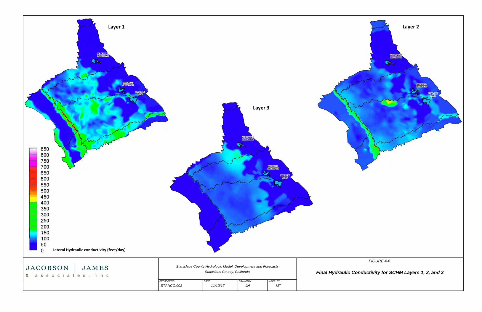
Stanislaus County Hydrologic Model: Development and Forecasts
Stanislaus County, California
FIGURE 4-6
Final Hydraulic Conductivity for SCHM Layers 1, 2, and 3
PROJECT NO.
STANCO.002
DATE
11/10/17
DRAWN BY
JH
APPR. BY
MT
Layer 1 Layer 2
Layer 3
Lateral Hydraulic conductivity (feet/day)

Stanislaus County Hydrologic Model: Development and Forecasts
Stanislaus County, California
FIGURE 4-7
Groundwater Level Elevations in SCHM Layers 1 and 2, September 2000
PROJECT NO.
STANCO.002
DATE
11/22/17
DRAWN BY
JH
APPR. BY
MT
Layer 1
Modeled Groundwater Level Elevation (feet above mean sea level)
Layer 2
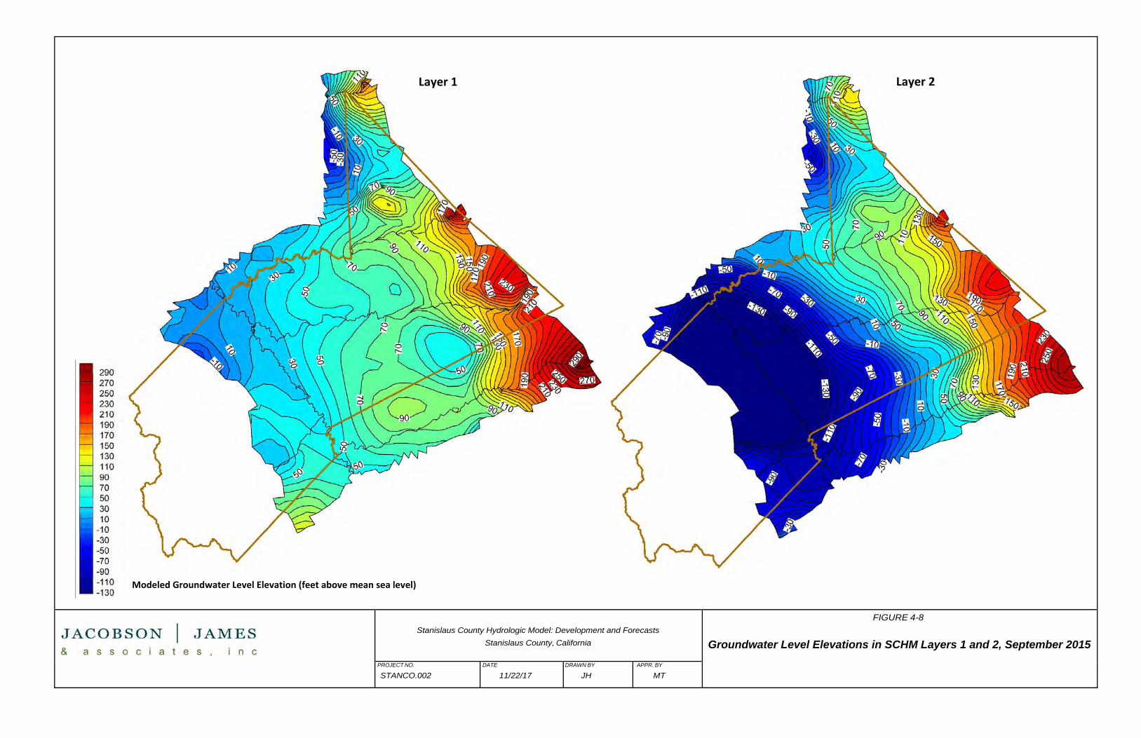
Stanislaus County Hydrologic Model: Development and Forecasts
Stanislaus County, California
FIGURE 4-8
Groundwater Level Elevations in SCHM Layers 1 and 2, September 2015
PROJECT NO.
STANCO.002
DATE
11/22/17
DRAWN BY
JH
APPR. BY
MT
Layer 1
Modeled Groundwater Level Elevation (feet above mean sea level)
Layer 2

Stanislaus County Hydrologic Model: Development and Forecasts December 20, 2017
Page 5-1
5.0 SENSITIVITY ANALYSIS
In order to investigate the sensitivity of the SCHM to variations in key parameters and inputs, a sensitivity
analysis was conducted by varying several key inputs as summarized in Table 5-1 below. The inputs were
varied across a range of low and high values, and the resulting simulated heads for September 2015 in Model
Layers 1 and 2 were compared the calibrated historical model. The purpose of this analysis was to provide
perspective on the significance of potential data gaps in the construction and calibration of the model, and to
help inform potential future model refinement efforts.
Table 5-1: Sensitivity Analysis Input Parameters
Model Input Range of Variation
Aquifer Layer Lateral Hydraulic Conductivity Existing Value x 0.2; Existing Value x 5
Storage Coefficients
- Specific Storage
- Specific Yield
Existing Value x 0.1; Existing Value x 10
Existing Value x 0.1; Existing Value x 2
Evapotranspiration Existing Value x 0.5; Existing Value x 2
Corcoran Clay Vertical Hydraulic Conductivity Existing Value x 0.2; Existing Value x 5
It should be noted that the ranges of input values listed above do not necessarily reflect an expected or
necessarily even a reasonable range in those parameters, but are a set of values intended to test the
sensitivity of the model to potential variations. The results of the analysis are discussed in the following
sections.
5.1 Aquifer Lateral Hydraulic Conductivity
The changes in simulated groundwater levels with decreased and increased model lateral hydraulic
conductivity are shown in Figures 5-1 and 5-2, respectively. As shown in Figure 5-1, decreasing model lateral
hydraulic conductivity has a significant but variable effect on simulated groundwater levels across the model
domain, increasing them in some areas while decreasing them in others. These results support the
observation that variations in hydraulic conductivity can affect model outcomes through multiple
mechanisms. In some areas, the primary effect of decreasing the hydraulic conductivity appears to be to slow
the flow of recharge away from an area and retain water in that part of the model, causing groundwater
mounding. This is observed in portions of the eastern foothill area of the model near the Stanislaus, Tuolumne

Stanislaus County Hydrologic Model: Development and Forecasts December 20, 2017
Page 5-2
and Merced Rivers, as well as in Layer 1 beneath areas east of the San Joaquin River that are irrigated primarily
through delivery of surface water. In other areas, lower hydraulic conductivity appears to result in greater
drawdown associated with simulated model pumping. In these areas, drawdown may also be increased as a
result of a slower rate of lateral groundwater inflow from recharge areas, such as in the cone of depression
beneath the eastern Turlock Subbasin, and in most of Layer 2, away from the foothills. In addition, in some
areas along the Diablo Range and the northern portion of the northeast model boundary, mountain front
recharge from small watersheds appears to be infiltrated less effectively, causing a local decline in simulated
groundwater levels.
As shown in Figure 5-2, increasing model lateral hydraulic conductivity also has a varying effect on simulated
groundwater levels, which is generally opposite of the effect of decreasing hydraulic conductivity
discussed above. With increased hydraulic conductivity, groundwater flows more readily away from recharge
areas and to areas where groundwater is extracted, decreasing drawdown in those areas.
These results may be most useful when considering the results of extensive evaluation of sediment texture
on hydraulic conductivity for the MERSTAN model (USGS, 2015). Regional adjustment of the end-point scaling
used in this analysis could be investigated to provide improvements in regional model calibration during
future refinements.
5.2 Storage Coefficients
The changes in simulated September 2015 groundwater level elevations with decreased and increased model
storage coefficients (Specific Storage and Specific Yield) are shown in Figures 5-3 and 5-4 respectively. As
shown in Figure 5-3, decreasing the model storage coefficients has the general effect of decreasing simulated
heads, and can also be a significant effect on model results. This is especially true in Layer 2 in the west central
portion of the model, which represents the confined aquifer system, and is consistent with less water being
available to be removed from storage for each increment of drawdown. This portion of the model represents
the model discharge area and reflects the cumulative effect of these changes throughout the model domain.
As shown in Figure 5-4, increasing model lateral storage coefficients has the opposite effect, except in some
isolated areas in the northeastern portion of the model domain. The reason for these local effects is not clear.
Local data regarding storage coefficients in the SCHM area are not widely available, and prior modeling efforts
have relied largely on generalized information and the results of regional studies. The analysis above
illustrates that the model could be refined if future model calibration efforts can rely on additional local field
data from aquifer tests.
5.3 Evapotranspiration
The changes in simulated September 2015 groundwater level elevations with decreased and increased model
evapotranspiration are shown in Figures 5-5 and 5-6 respectively. As shown in Figure 5-5, decreasing the
model evapotranspiration has the general effect of increasing simulated heads. This is true across the model
domain in both Layers 1 and 2, but is most pronounced in the western portion of Layer 2 where the

Stanislaus County Hydrologic Model: Development and Forecasts December 20, 2017
Page 5-3
cumulative effects of more water being available for deep percolation throughout the model domain become
more pronounced. As shown in Figure 5-6, increasing model evapotranspiration has the opposite effect,
resulting in a decrease in heads across the model domain in both Layers 1 and 2. Similar to decreasing
evapotranspiration, the cumulative effects of less deep percolation being available throughout the model
domain become most pronounced in western portion of Layer 2.
These results reflect the fact that evapotranspiration from crops and natural vegetation is a significant
component of the model water budget. DWR is undertaking efforts to refine its understanding of
evapotranspiration in cropping in the region through several remote-sensing datasets. The results of these
efforts were not available during development of the SCHM, but will be available to inform future
modeling efforts.
5.4 Aquitard Vertical Hydraulic Conductivity
The changes in simulated September 2015 groundwater level elevations with decreased and increased
Corcoran Clay vertical hydraulic conductivity are shown in Figures 5-7 and 5-8 respectively. As shown in Figure
5-7, decreasing the Corcoran Clay vertical hydraulic conductivity has the general effect of increasing simulated
heads in Layer 1 and decreasing heads in Layer 2 beneath the Corcoran Clay subcrop area. This is because
water is retained in the upper aquifer system and vertical leakance into the underlying confined aquifer
system if impeded. This is effect is most pronounced in the western portion of the model, west of the San
Joaquin River. As shown in Figure 5-8, increasing the vertical hydraulic conductivity has the opposite effect,
resulting in a decrease in simulated heads in Layer 1 and an increase in simulated heads in Layer 2 beneath
the Corcoran Clay subcrop area. This is because more water is allowed to leak vertically out of Layer 1 and
into Layer 2 in this area.
These results illustrate the fact that the Corcoran Clay is a key regional hydrostratigraphic unit that affects not
only the aquifer system’s response to shallow and deep pumping, but also to the partition of the groundwater
budget between the shallow and deep aquifer system. Local data regarding the vertical hydraulic conductivity
of this unit are sparse, and prior modeling efforts have relied largely on regional studies or calibration results
to assign values to this important parameter. The model could be refined through targeted evaluation of this
important input parameter.

Stanislaus County Hydrologic Model: Development and Forecasts
Stanislaus County, California
FIGURE 5-1
Sensitivity Analysis Results:
Decreased Lateral Hydraulic Conductivity PROJECT NO.
STANCO.002
DATE
11/22/17
DRAWN BY
JH
APPR. BY
MT
Head Difference after Hydraulic Conductivity Decrease (0.2 x) (feet)
Layer 1 Layer 2

Stanislaus County Hydrologic Model: Development and Forecasts
Stanislaus County, California
FIGURE 5-2
Sensitivity Analysis Results:
Increased Lateral Hydraulic Conductivity PROJECT NO.
STANCO.002
DATE
11/22/17
DRAWN BY
JH
APPR. BY
MT
Layer 1
Head Difference after Hydraulic Conductivity Increase (5x) (feet)
Layer 2

Stanislaus County Hydrologic Model: Development and Forecasts
Stanislaus County, California
FIGURE 5-3
Sensitivity Analysis Results:
Decreased Storage Coefficients PROJECT NO.
STANCO.002
DATE
11/22/17
DRAWN BY
JH
APPR. BY
MT
Layer 1
Head Difference after Storage Coefficient Decrease (Ss and Sy x 0.1) (feet)
Layer 2
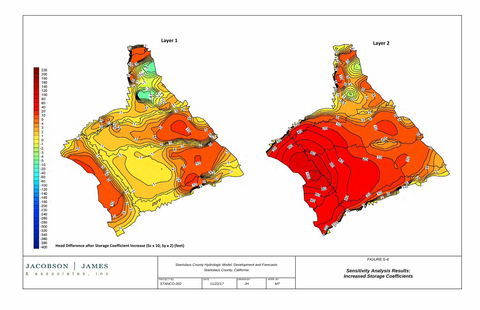
Stanislaus County Hydrologic Model: Development and Forecasts
Stanislaus County, California
FIGURE 5-4
Sensitivity Analysis Results:
Increased Storage Coefficients PROJECT NO.
STANCO.002
DATE
11/22/17
DRAWN BY
JH
APPR. BY
MT
Layer 1
Head Difference after Storage Coefficient Increase (Ss x 10; Sy x 2) (feet)
Layer 2

Stanislaus County Hydrologic Model: Development and Forecasts
Stanislaus County, California
FIGURE 5-5
Sensitivity Analysis Results:
Decreased Evapotranspiration PROJECT NO.
STANCO.002
DATE
11/22/17
DRAWN BY
JH
APPR. BY
MT
Layer 1
Head Difference after Evapotranspiration Decrease (ET x 0.5) (feet)
Layer 2

Stanislaus County Hydrologic Model: Development and Forecasts
Stanislaus County, California
FIGURE 5-6
Sensitivity Analysis Results: Increased Evapotranspiration
PROJECT NO.
STANCO.002
DATE
11/22/17
DRAWN BY
JH
APPR. BY
MT
Layer 1
Head Difference after Evapotranspiration Increase (ET x 2) (feet)
Layer 2

Stanislaus County Hydrologic Model: Development and Forecasts
Stanislaus County, California
FIGURE 5-7
Sensitivity Analysis Results:
Decreased Aquitard Vertical Hydraulic Conductivity PROJECT NO.
STANCO.002
DATE
11/22/17
DRAWN BY
JH
APPR. BY
MT
Layer 1
Head Difference after Corcoran Clay Hydraulic Conductivity Decrease (Kv x 0.2) (feet)
Layer 2
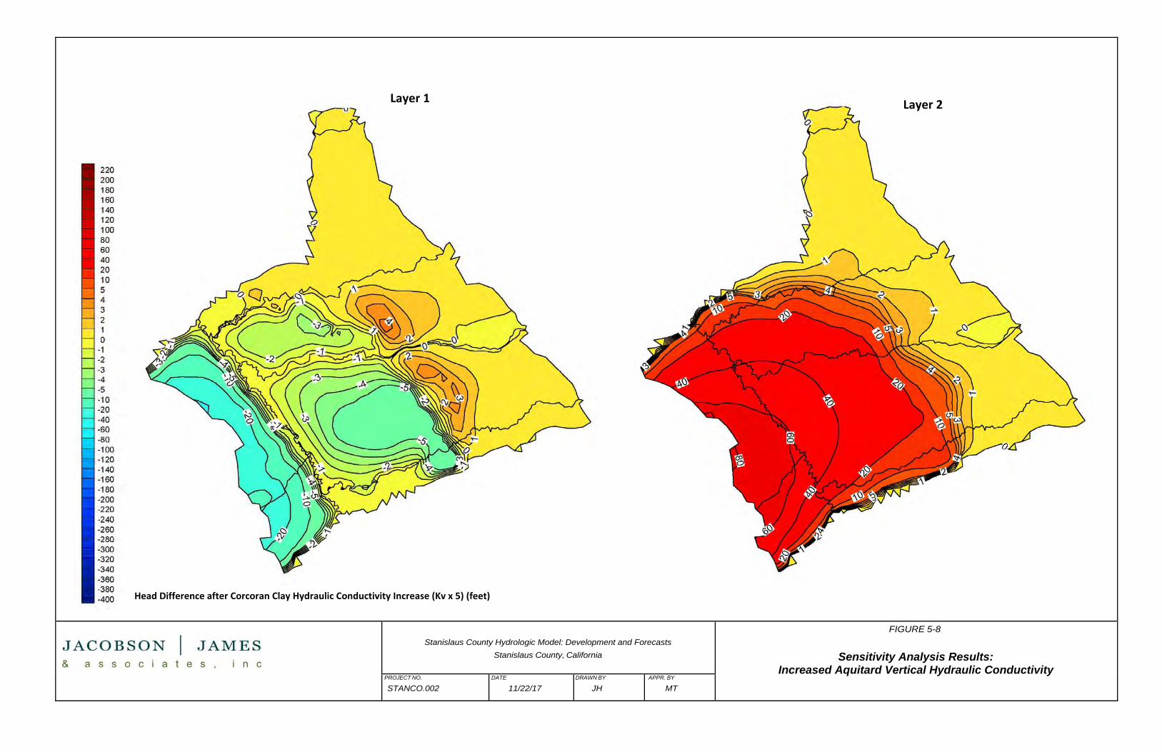
Stanislaus County Hydrologic Model: Development and Forecasts
Stanislaus County, California
FIGURE 5-8
Sensitivity Analysis Results:
Increased Aquitard Vertical Hydraulic Conductivity PROJECT NO.
STANCO.002
DATE
11/22/17
DRAWN BY
JH
APPR. BY
MT
Layer 1
Head Difference after Corcoran Clay Hydraulic Conductivity Increase (Kv x 5) (feet)
Layer 2

Stanislaus County Hydrologic Model: Development and Forecasts December 20, 2017
Page 6-1
6.0 MODEL FORECASTS
6.1 Approach
Model forecasts were run from 2016 through 2042 to provide perspective on the effects of potential future
groundwater management trends, and to evaluate the impacts of discretionary well permitting at a
programmatic level. Several key uncertainties underlie these scenarios: (1) GSPs for the subbasins in the
Study Area have not yet been prepared and, as such, sustainable yields and management criteria remain to
be established; (2) Important water policy decisions that could profoundly affect groundwater management
in the region are currently pending (SWRCB, 2016); and, (3) The actual locations of wells that will be permitted
under the County’s discretionary well permitting program are not known. For these reasons, it is important
to note that the simulated scenarios described below are not deterministic, quantitative assessments, but are
intended to provide perspective on the reasonable range of potential outcomes, and to inform the evaluation
of whether a potential exists for significant impacts to result from the permitting of discretionary wells by the
County. The scenarios evaluated in this study are described in Table 6-1. Additional details regarding the
approach used and the results of the simulations are presented in Sections 6.2 through 6.6, below.
6.2 Scenario 1 – Baseline
Scenario 1 provides the basic hydrologic conditions for each of the subsequent scenarios, and is the baseline
against which Scenarios 2 through 5 are compared to assess the changes produced by the scenario
assumptions using a superposition approach. The following approach was used to construct this scenario.
• Scenario 1 includes a sequence of historical hydrologic years assembled to represent a reasonable
sequence of future hydrologic conditions. The selected years and their hydrologic year type based
on the San Joaquin Valley Water Year Hydrologic Classification Index (DWR, 2017a) are presented on
Figure 6-1. The hydrologic data used includes surface water inflows, precipitation and temperature/
evapotranspiration. Gridded PRISM data (Daly et al., 2004) for precipitation, where a mix of real
years were associated with corresponding model years, were prepared as input for the SCHM grid.
• Surface water diversions for the forecast hydrologic years were developed for the baseline scenario
using the approach summarized in Table 3-2. When the historical hydrologic years used to develop
the forecast sequence preceded WY 1991, a representative year between WY 1991 and WY 2015
with a similar hydrology for which diversions were developed was utilized to represent diversions.
• Climate change was incorporated into the baseline scenario by assuming similar precipitation as
historical conditions, and allowing for an increase in temperature. The temperature increase was
associated with an increase in evapotranspiration that was calculated in input into the model.
Evapotranspiration changes resulted from a steady increase in temperature of 0.0355 degrees Celsius
(oC) per year from WY 2016 through WY 2042. The selected temperature ramp is based on an
extrapolation using recent trends in historical data for California, over 1970-2006, using US Historical
Climate Network and National Weather Service Cooperative Network data for the San Joaquin basin

Stanislaus County Hydrologic Model: Development and Forecasts December 20, 2017
Page 6-2
(Cordero et al., 2011). The specific value is the mean statistically significant increase for the daily
minimum and daily maximum temperature at individual stations. This temperature change was used
to calculate corresponding evapotranspiration changes using a variation of the Penman Equation
developed by Makkink (Makkink, 1957),9 and to develop multipliers to adjust monthly
evapotranspiration values in the model Evapotranspiration Data file of C2VSim.
• In order to allow Scenario 1 to be used as a baseline for the evaluation of potential future
groundwater management and demand changes, the groundwater demand simulated in this
scenario is based on the assumption that WY 2015 urban demand will continue, WY 2015 land use
patterns will be maintained throughout the forecast period, and WY 2015 time-dependent boundary
conditions will be maintained.
6.3 Scenario 2 – Reasonable Upper Bound Potential Demand Increase
The municipal water demand increase simulated in this scenario was developed using water demand
forecasts contained in UWMPs developed for the region as summarized in Table 6-2. As summarized in this
table, the average median annual urban water demand increase in the region is approximately 2.7%.10
This factor was used for all cities except Modesto. For Modesto, the mean forecast demand increase through
2040 is 0.08%; however, this average includes an initial forecast demand decline, and a forecast increase of
0.4% per year was therefore applied. Rural domestic groundwater demand was assumed to increase in
proportion to a rural population growth rate of approximately 1 percent per year.
It is reasonable to assume that any increase in urban water demand and delivery would be associated with a
corresponding increase in recharge from urban return flows, and from retirement of agricultural demand as
parcels are converted for urban use. For this scenario, it was assumed that the projected demand increase
represents a reasonable maximum net pumping increase that includes any offsetting agricultural demand
reduction, and the associated return flow and deep percolation were not explicitly modeled.
Also simulated in this scenario is an increase in agricultural groundwater demand resulting from the
conversion of unincorporated rangeland in the eastern portion of the county to irrigated agricultural land.
The forecast rate of agricultural land conversion in Scenario is based on the historical rate of rangeland
conversion to permanent crops in the eastern portion of the County between 2000 and 2015 reported by the
Stanislaus County Agricultural Commissioner (Appendix A). Based on this information, it is assumed that
3,100 acres per year of rangeland in this area is converted to orchard.
Drawdowns predicted in Layers 1 and 2 in 2022 and 2042 under Scenario 2 are shown graphically in Figures
6-2 and 6-3, and key water budget changes are summarized in Table 6-3. These results are presented as
9 Tetra Tech performed a study comparing six different methods to calculate evapotranspiration based on changes in temperature alone. The method of Makkink provided the best correlation with measured values and was adopted for use in developing the SCHM. 10 This average includes data from UWMPs that predate as well as postdate the requirements of SBX7-7 in order to develop a reasonable maximum urban demand growth scenario. As such, the estimate was not developed to explicitly simulate current municipal water conservation/demand reduction requirements.

Stanislaus County Hydrologic Model: Development and Forecasts December 20, 2017
Page 6-3
changes relative to the baseline case (Scenario 1). Changes induced by increasing municipal and agricultural
groundwater demand under this scenario include the following:
• Under this scenario, drawdown in Layer 1 (the shallow aquifer system) in the eastern foothills area
of the SCHM is predicted to range from approximately 1 to 3 feet by 2022 and approximately 5 to 30
feet by 2042. The lateral expansion of drawdown cones is limited by the major groundwater-
connected streams draining the foothills, including the Stanislaus, Tuolumne and Merced Rivers.
This is consistent with an increase in the amount of streamflow lost to groundwater as shown in
Table 6-3. Drawdown in Layer 2 (the deeper aquifer system) in the eastern portion of the SCHM is
predicted to range from approximately 1 to 5 feet in 2022 and approximately 10 to 40 feet in 2042.
• Groundwater levels in Layer 1 beneath Turlock and Patterson are predicted to rise between 1 and 2
feet by 2042. The rise in groundwater levels occurs because municipal pumping in these areas occurs
primarily from the deeper aquifer system (Layer 2); whereas deep percolation from urban water use
will be a source of recharge to Layer 1. In reality, a greater amount of net recharge to the shallow
aquifer system may occur as a result of the conversion of agricultural land to urban land, and the
retirement of agricultural water demand.
• Cones of depression are predicted to form in Layer 1 beneath urban areas that rely more extensively
on groundwater from the shallow aquifer system (e.g., Modesto, Riverbank, Hughson and Oakdale).
Layer 1 groundwater levels are predicted to fall by approximately 1 to 3 feet beneath these cities by
2042.
• A broad cone of depression is predicted to form in Layer 2, centered approximately on the Cities of
Turlock and Patterson. Drawdowns beneath Turlock are predicted to range from 1 to 4 feet by 2022,
and 10 to 20 feet by 2042. Drawdowns beneath Patterson are predicted to exceed 1 foot by 2022,
and to range from 5 to 10 feet by 2042.
• Consistent with the observation above regarding apparent streamflow depletion due to pumping
under Scenario 2, forecast water budget data (Table 6-3) indicates net groundwater discharge to
streams from the Eastern San Joaquin, Modesto and Turlock Subbasins is forecast to decrease
several thousand AFY (approximately 0.6 & to 2 %) by 2022 and several tens of thousands AFY
(approximately 4% to 13 %) by 2042, relative to the baseline case. Groundwater discharge from the
Delta Mendota Subbasin to streams is not predicted to change significantly (less than 0.2 %).
• As summarized in Table 6-3, the cumulative groundwater storage change in the Eastern San Joaquin,
Modesto and Turlock Subbasins is forecast to decrease several thousand AF (approximately 0.1 %)
by 2022 and several tens of thousand AF (approximately 0.4 % to 1.8 %) by 2042, relative to the
baseline case. Groundwater storage change in the Delta Mendota Subbasin is not predicted to vary
significantly from the baseline change.
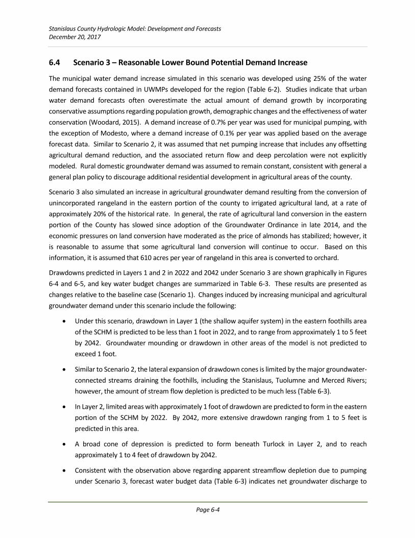
Stanislaus County Hydrologic Model: Development and Forecasts December 20, 2017
Page 6-4
6.4 Scenario 3 – Reasonable Lower Bound Potential Demand Increase
The municipal water demand increase simulated in this scenario was developed using 25% of the water
demand forecasts contained in UWMPs developed for the region (Table 6-2). Studies indicate that urban
water demand forecasts often overestimate the actual amount of demand growth by incorporating
conservative assumptions regarding population growth, demographic changes and the effectiveness of water
conservation (Woodard, 2015). A demand increase of 0.7% per year was used for municipal pumping, with
the exception of Modesto, where a demand increase of 0.1% per year was applied based on the average
forecast data. Similar to Scenario 2, it was assumed that net pumping increase that includes any offsetting
agricultural demand reduction, and the associated return flow and deep percolation were not explicitly
modeled. Rural domestic groundwater demand was assumed to remain constant, consistent with general a
general plan policy to discourage additional residential development in agricultural areas of the county.
Scenario 3 also simulated an increase in agricultural groundwater demand resulting from the conversion of
unincorporated rangeland in the eastern portion of the county to irrigated agricultural land, at a rate of
approximately 20% of the historical rate. In general, the rate of agricultural land conversion in the eastern
portion of the County has slowed since adoption of the Groundwater Ordinance in late 2014, and the
economic pressures on land conversion have moderated as the price of almonds has stabilized; however, it
is reasonable to assume that some agricultural land conversion will continue to occur. Based on this
information, it is assumed that 610 acres per year of rangeland in this area is converted to orchard.
Drawdowns predicted in Layers 1 and 2 in 2022 and 2042 under Scenario 3 are shown graphically in Figures
6-4 and 6-5, and key water budget changes are summarized in Table 6-3. These results are presented as
changes relative to the baseline case (Scenario 1). Changes induced by increasing municipal and agricultural
groundwater demand under this scenario include the following:
• Under this scenario, drawdown in Layer 1 (the shallow aquifer system) in the eastern foothills area
of the SCHM is predicted to be less than 1 foot in 2022, and to range from approximately 1 to 5 feet
by 2042. Groundwater mounding or drawdown in other areas of the model is not predicted to
exceed 1 foot.
• Similar to Scenario 2, the lateral expansion of drawdown cones is limited by the major groundwater-
connected streams draining the foothills, including the Stanislaus, Tuolumne and Merced Rivers;
however, the amount of stream flow depletion is predicted to be much less (Table 6-3).
• In Layer 2, limited areas with approximately 1 foot of drawdown are predicted to form in the eastern
portion of the SCHM by 2022. By 2042, more extensive drawdown ranging from 1 to 5 feet is
predicted in this area.
• A broad cone of depression is predicted to form beneath Turlock in Layer 2, and to reach
approximately 1 to 4 feet of drawdown by 2042.
• Consistent with the observation above regarding apparent streamflow depletion due to pumping
under Scenario 3, forecast water budget data (Table 6-3) indicates net groundwater discharge to

Stanislaus County Hydrologic Model: Development and Forecasts December 20, 2017
Page 6-5
streams from the Eastern San Joaquin, Modesto and Turlock Subbasins is forecast to decrease by
about 1,000 AFY each (approximately 0.1 % to 0.4 %) by 2022 and several thousand AFY
(approximately 0.7 % to 2.5 %) by 2042, relative to the baseline scenario. Groundwater discharge
from the Delta Mendota Subbasin to streams is not predicted to change significantly from the
baseline.
• As summarized in Table 6-3, the cumulative groundwater storage change in the Eastern San Joaquin,
Modesto and Turlock Subbasins is forecast to decrease by about 1,000 AFY each by 2022 and several
thousand AFY by 2042. Groundwater storage change in the Delta Mendota Subbasin is not predicted
to vary significantly from the baseline.
6.5 Scenario 4 – Discretionary Well Permitting
Scenario 4 was constructed to evaluate the potential effects of permitting new discretionary wells under the
County Groundwater Ordinance. This was accomplished by randomly selecting 10 model elements each year
starting in 2018 for simulation of pumping from a new well that would theoretically be installed under the
Ordinance. Ten wells per year is considered a reasonable maximum for this evaluation, based on the
observation that only two discretionary wells have been processed for permitting during the first three years
since the Ordinance was adopted in November 2014. Even if the rate of well permitting increases after
adoption of the PEIR in early 2018, it appears unlikely that more than 10 wells per year will be permitted on
average. Each well is assumed to extract approximately 400 AFY of groundwater from Layer 1 (Scenario 4a)
or Layer 2 (Scenario 4b). The wells are assumed to be installed in unincorporated, non-district lands
throughout the County from 2018 to 2020, and in unincorporated lands of the Modesto and Turlock Subbasin
from 2021 to 2022, based on schedule mandated schedule for adoption of GSPs. The locations and
installation years for the simulated wells are shown on Figure 6-6.
Drawdowns induced in Layers 1 and 2 in 2022 and 2042 are shown graphically in Figure 6-7 and 6-8 for
Scenario 4a, and Figures 6-9 and 6-10 for Scenario 4b. Key water budget changes for Scenarios 4a and 4b are
summarized in Table 6-3. These results are presented as changes relative to the baseline case.
Changes predicted to be induced by discretionary well permitting under Scenarios 4a (shallow wells) include
the following:
• Cones of depression are predicted to develop in the eastern portion of the County in Layer 1, with
drawdown ranging from 1 to 5 feet by 2022. By 2042 these cones of depression are predicted to
expand and deepen to approximately 4 to 10 feet. The lateral expansion of drawdown cones is
predicted to be limited by the Stanislaus and Tuolumne Rivers, from which the wells would derive at
least some of their extracted groundwater, as summarized in Table 6-3. Smaller, local cones of
depression are also predicted to form where wells are located in other areas of the County; however,
these cones of are predicted to be more limited in size and depth, remaining between 1 and 2 feet
in depth throughout the entire simulation. This distribution of drawdown is consistent with a greater
degree of groundwater development and limited recharge in the eastern portion of the County.

Stanislaus County Hydrologic Model: Development and Forecasts December 20, 2017
Page 6-6
• Drawdown in Layer 2 is predicted to be more muted. Predicted drawdown exceeding 1 foot is limited
to the eastern portion of the County. In this area, several cones of depression are predicted to reach
drawdowns from 1 to 3 feet. Similar to Layer 1, this drawdown is predicted to expend by 2042, and
to range from 1 to 5 feet by that time.
• Consistent with the observation above regarding apparent streamflow depletion due to pumping
under Scenario 4a, forecast water budget data (Table 6-3) indicates net groundwater discharge to
streams from the Delta-Mendota, Eastern San Joaquin, Modesto and Turlock Subbasins is forecast
to decrease by about 3,400, 1,400 to 9,000 and 2,900 AFY (approximately 0.6 % to 1.7 %),
respectively, by 2022, and 4,000, 2,900, 13,000 and 3,100 AFY (approximately 0.6 % top 1 %),
respectively, by 2042, relative to the baseline scenario.
• As summarized in Table 6-3, cumulative groundwater storage change in the Delta-Mendota, Eastern
San Joaquin, Modesto and Turlock Subbasins is forecast to decrease by about 1,000 to 4,000 AF
(approximately 0.1 % or less) by 2022. Storage depletion rates are forecast to decrease over time.
By 2042, cumulative storage depletion in the Eastern San Joaquin Subbasin is predicted to be
approximately 1,300 AFY (approximately 0.3 %) less than the baseline, and be essentially unchanged
from the baseline in the other subbasins. In addition, the annual rate of storage change in the
subbasins is predicted to be low (less than 0.01 %) with the basins remaining relatively stable.
Changes predicted to be induced by discretionary well permitting under Scenarios 4b (deeper wells) include
the following:
• As expected, the development of cones of depression in the upper aquifer system (Layer 1) for
Scenario 4b (deeper wells) is predicted to be more muted than under Scenario 4a. Cones of
depression are predicted to develop in the eastern portion of the County with drawdown ranging
from 1 to 3 feet by 2022 and 3 to 5 feet by 2042. As in Scenario 4a, lateral propagation of drawdown
appears to be limited by the Stanislaus and Tuolumne Rivers. Smaller cones of depression up to
between 1 and 2 feet in depth are predicted to form in the central portion of the County by 2022
but are not predicted to grow further in size.
• In the deeper aquifer system (Layer 2), drawdown is predicted to be somewhat more extensive
under Scenario 4b. A series of depression cones under the eastern portion of the County is predicted
to reach a depth of 2 to 5 feet by 2022 and 3 to 6 feet by 2042. In addition, a broad area of drawdown
is predicted to form in the confined aquifer system beneath the western portion of the County and
to reach a depth of approximately 5 feet in 2022. Although the area of drawdown is predicted to
grow by 2042, it is not predicted to get deeper.
• As summarized in Table 6-3, streamflow depletion under this scenario is predicted to be similar to,
or somewhat less than, streamflow depletion rates under Scenario 4a. Groundwater storage
depletion rates are predicted to be generally similar for the two scenarios, although cumulative
depletion, on average, is predicted to be higher for Scenario 4b.

Stanislaus County Hydrologic Model: Development and Forecasts December 20, 2017
Page 6-7
6.6 Scenario 5 – Additional Surface Water Delivery
Scenario 5 evaluates the potential effect of additional surface water deliveries to offset municipal demand.
This scenario was developed using the demand growth simulated in Scenario 2, and groundwater level
changes were evaluated relative to Scenario 1. Additional surface water deliveries were simulated using the
currently planned Stanislaus Regional Water Authority (SWRA) project as a surrogate. It should be noted that
this evaluation is intended to provide perspective on the potential effects of conjunctive use projects to help
meet municipal water demand in the region, but actual evaluation of the impacts and benefits of the SRWA
will require more in-depth analysis. To construct the water demand inputs for this scenario, it was assumed
that up to 5,700 AFY of Tuolumne River water will be supplied to the City of Ceres and up to 11,100 AFY will
be supplied to the City of Turlock, beginning in 2022 (West Yost, 2017). The point of diversion will be just
downstream of the Greer Road bridge. The minimum groundwater extraction rates assumed to be needed
to maintain the water quality and functionality of existing supply wells is assumed to be 2 million gallons/day
(MGD) in Ceres and 6.6 MGD in Turlock (West Yost, 2016). During the winter months (assumed to be
December through March), as much of the demand as possible will be supplied from surface water and
groundwater pumping will be decreased to minimum levels. During the rest of the year, groundwater
pumping may be increased above minimum levels, if needed to meet peak demands.
Scenario 5 maintained an increase in agricultural groundwater demand resulting from the conversion of
unincorporated rangeland in the eastern portion of the county to irrigated agricultural land, at a rate of 3,100
acres per year.
Drawdowns predicted in Layers 1 and 2 in 2022 and 2042 under Scenario 5 are shown graphically in Figures
6-11 and 6-12, and key water budget changes are summarized in Table 6-3. These results are presented as
changes relative to the baseline case (Scenario 1). Changes induced by increasing municipal and agricultural
water demand and adding conjunctive use to meet the municipal demand under this scenario include
the following:
• Under this scenario, predicted drawdown in Layer 1 (the shallow aquifer system) and Layer 2 in the
eastern foothills area of the SCHM remains essentially unchanged from Scenario 2. Drawdowns
predicted in the Delta-Mendota Subbasin near the City of Patterson are somewhat muted compared
to Scenario 2, but are generally similar.
• In the western Turlock Subbasin beneath Turlock, groundwater levels are predicted to rise up to 1 to
2 feet by 2022 and up to 5 feet by 2042. Beneath the City of Patterson, groundwater levels are
predicted to rise between 1 and 2 feet by 2042. As would be expected, the groundwater level rise
under this scenario is greater than under Scenario 2, which simulates reasonable maximum
groundwater demand growth.
• Groundwater levels in Layer 2 beneath the western Turlock Subbasin are also predicted to rise
initially, reaching up to 4 feet above the baseline case. By 2042, however, groundwater levels are
predicted to fall to elevations that are up to 10 feet below the baseline case. This is compared to
drawdowns under Scenario 2 in the range of 1 to 4 feet by 2022, and 10 to 20 feet by 2042. As such,
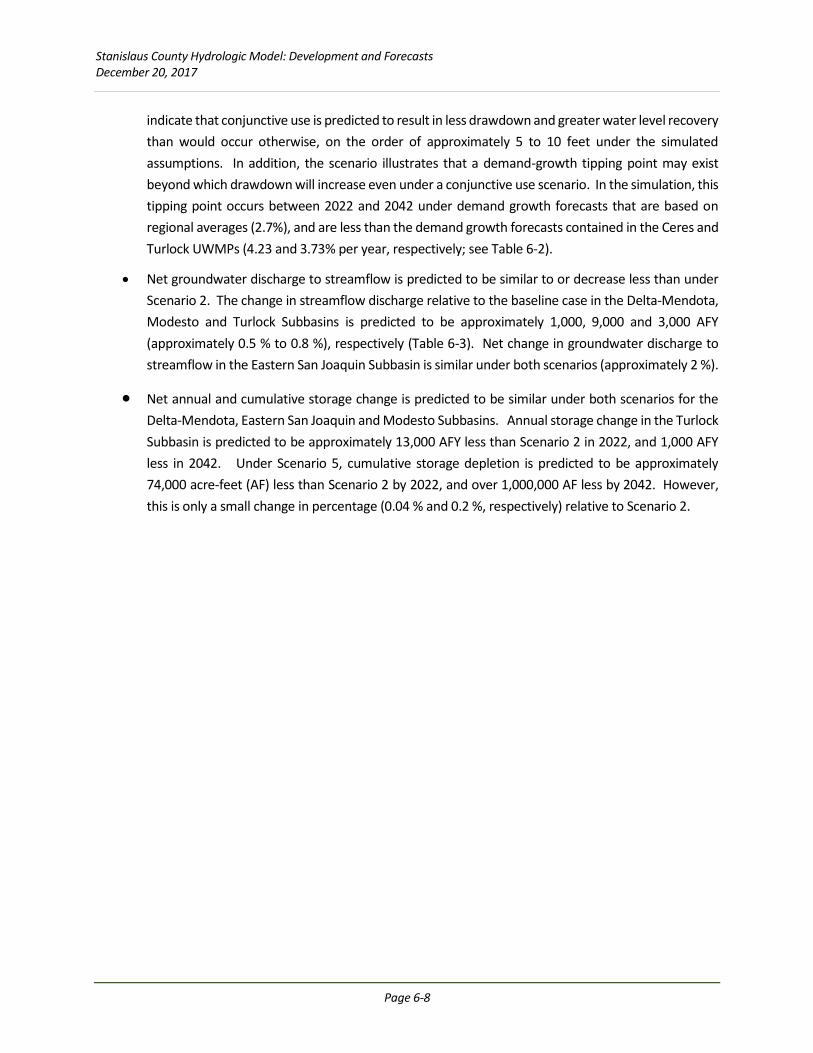
Stanislaus County Hydrologic Model: Development and Forecasts December 20, 2017
Page 6-8
indicate that conjunctive use is predicted to result in less drawdown and greater water level recovery
than would occur otherwise, on the order of approximately 5 to 10 feet under the simulated
assumptions. In addition, the scenario illustrates that a demand-growth tipping point may exist
beyond which drawdown will increase even under a conjunctive use scenario. In the simulation, this
tipping point occurs between 2022 and 2042 under demand growth forecasts that are based on
regional averages (2.7%), and are less than the demand growth forecasts contained in the Ceres and
Turlock UWMPs (4.23 and 3.73% per year, respectively; see Table 6-2).
• Net groundwater discharge to streamflow is predicted to be similar to or decrease less than under
Scenario 2. The change in streamflow discharge relative to the baseline case in the Delta-Mendota,
Modesto and Turlock Subbasins is predicted to be approximately 1,000, 9,000 and 3,000 AFY
(approximately 0.5 % to 0.8 %), respectively (Table 6-3). Net change in groundwater discharge to
streamflow in the Eastern San Joaquin Subbasin is similar under both scenarios (approximately 2 %).
• Net annual and cumulative storage change is predicted to be similar under both scenarios for the
Delta-Mendota, Eastern San Joaquin and Modesto Subbasins. Annual storage change in the Turlock
Subbasin is predicted to be approximately 13,000 AFY less than Scenario 2 in 2022, and 1,000 AFY
less in 2042. Under Scenario 5, cumulative storage depletion is predicted to be approximately
74,000 acre-feet (AF) less than Scenario 2 by 2022, and over 1,000,000 AF less by 2042. However,
this is only a small change in percentage (0.04 % and 0.2 %, respectively) relative to Scenario 2.

TABLE 6‐1SCHM FORWARD MODELING SCENARIOS
Stanislaus County Hydrologic Model: Development and Forecast ModelingStanislaus County, California
Scenario Purpose Description and Assumptions ApproachUse the hydrology data series outlined in Figure 6‐1 to simulate forecast hydrologic conditions.Use the approach outlined in Table 3‐2 develop a diversion dataset.
Escalate evapotranspiration using the Makkink method based on a temperature increase of 0.0355 ᵒC/year.
Maintain municipal and rural domestic demand at 2015 levels.Maintain 2015 cropping and land use patterns.Use the baseline data from Scenario 1 as a starting and comparison point.
Increase municipal pumping by 2.7 %/year (median average UWMP demand increase) for all cities except Modesto.
Increase municipal pumping in Modesto by 0.4%/year.Increase rural domestic pumping by 1%/year.Demand increase offset by land use conversion is captured in pumping rate adjustment.Convert Natural Vegetation land to Agricultural Land (orchards) in unincorporated, non‐district areas, EWD and BCWD at a rate of 3,100 acres/year.Use the baseline data from Scenario 1 as a starting and comparison point.Increase municipal pumping by 0.7 %/year (25 % of median average UWMP demand increase) for all cities except Modesto.Increase municipal pumping in Modesto by 0.1%/year.Demand increase offset by land use conversion is captured in pumping rate adjustment.Convert Natural Vegetation land to Agricultural Land (orchards) in unincorporated, non‐district areas, EWD and BCWD at a rate of 610 acres/year (20% of historical rate from 2000 to 2015).
Use the baseline data from Scenario 1 as a starting and comparison point.
Add the wells shown in Figure 6‐6, which were selected in the centers of randomly selected elements in unincorporated, non‐district lands in the eastern foothills.Add the wells to either Model Layer 1 (Scenario 4a) or Model Layer 2 (Scenario 4b) in the sequence indicated on Figure 6‐6. Specify pumping for the wells at a rate of 400 AFY (assuming a typical demand of 4 feet for a typical 100‐acre orchard for each well).Use the baseline data from Scenario 2 as a starting point and compare to Scenario 1.Model diversion of up to 5,600 AFY surface water from the Tuolumne River downstream of Geer Road to City of Ceres starting 2022 (West Yost, 2017), and decrease municipal pumping proportionally. Decrease well pumping to no less than 2 mgd and increase well pumping in April‐November as needed to meet Scenario 2 demand (West Yost 2016).Model diversion of up to 11,100 AFY surface water from the Tuolumne River downstream of Geer Road to City of Turlock starting 2022 (West Yost, 2017), and decrease municipal pumping proportionally. Decrease well pumping to no less than 6.6 mgd and increase well pumping in April‐November as needed to meet Scenario 2 demand (West Yost 2016).
Notes:AFY = acre foot per yearBCWD = Ballico‐Cortez Water DistrictEWD = Eastside Water DistrictGSP = Groundwater Sustainability Planmgd = million gallon per dayPEIR = Programmatic Environmental Impact ReportUWMP = Urban Water Management PlanᵒC = degree Celsius% = percent
Sources:West Yost, 2016. Preliminary Phasing and Water Treatment Plant Sizing for the SRWA Surface Water Supply Project. June 16. West Yost, 2017. Surface Water Supply Project, Initial Project Capacity, Estimated Cost and Rate Impacts. Presentation for Stanislaus Regional Water Authority. August 3.
Scenario 3 – Reasonable Lower Bound Potential Demand Increase
Provide perspective on the effectiveness of limiting the expansion of groundwater extraction to decrease potential effects of agricultural and municipal groundwater demand increases. This scenarios is to represent a lower bound of reasonable demand growth.
Agricultural conversion in the east foothills is assumed to proceed at a rate that is approximately 20% of historical rates, consistent with recent slowdowns in the planting of new orchards in this area. Urban demand is assumed to increase at a rate that approximately 25% of forecast rates. This assumption assumes that UWMP demand forecasts may be overly conservative, that additional efficiency improvements will be implemented, and that some demand increase will be offset by urban development of agricultural land. In the case of Modesto, it is assumed that unused agricultural deliveries will be made available to meet municipal demand. Rural domestic demand is assumed not to grow, consistent with an existing General Plan policy to limit rural residential development.
Scenario 1 ‐ BaselineEstablishes a baseline against which the other scenarios are compared.
Prepare a sequence years that will represent the hydrology dataset for forecasts. Use historical data to represent a representative sequence of normal, wet and dry years. Maintain 2015 groundwater demand and cropping patterns throughout the baseline forecast period. Incorporate climate change into the hydrology dataset by developing a temperature ramp based on published data and calculating the resulting evapotranspiration increases for input into the model. Use the resulting dataset as a comparison point for all of the subsequent scenarios.
Scenario 2 – Reasonable Upper Bound Potential Demand Increase
Provide perspective on potential effects if agricultural groundwater demand grows at historical rates and municipal demand grows at rates forecast in UWMPs. This scenario is to represent an upper bound of reasonable demand growth.
Agricultural water demand is assumed to increase through the continued conversion of rangeland in the eastern foothill region at rates experienced from 2000 to 2015. Urban water demand is assumed to increase in accordance with water demand increases forecast in UWMPs, and to be offset to some degree with the conversion of remaining agricultural land to urban use. Rural domestic water demand is assumed to increase at forecast population growth rates in the Stanislaus County General Plan Housing Element.
Scenario 5 – Additional Surface Water Delivery
Evaluate the potential effectiveness of making additional surface water available to meet municipal water demand in the County.
Model delivery of additional surface water to Turlock and Ceres to simulate the general effect of projects such as the Stanislaus Regional Water Authority project on groundwater levels and budgets. Use Scenario 2 – Reasonable Upper Bound Potential Demand Increase as a starting point to compare effectiveness against.
Add 10 new wells per year at randomly selected locations in unincorporated, non‐district lands within the County between 2018 and 2020, then continue adding 10 wells per year from 2021 to 2022, but only in the Modesto and Turlock Subbasins. The timing of adding new wells is consistent with the time frame during which discretionary well permitting will occur prior to the adoption of GSPs in 2020 in the Eastern San Joaquin and Delta‐Mendota Subbasins, and in 2022 in the Modesto and Turlock Subbasins. Ten wells per year are assumed to be added as an estimated upper bound assuming that the rate of discretionary well permitting will increase after completion of the PEIR. Note that since the Ordinance was adopted in November 2014, only two discretionary well permits have been processed; however, over 1,000 non‐discretionary well permits were processed in the same time frame, indicating a back log of demand for well permits may exist.
Evaluate the potential effects of permitting new extraction wells subject to the Groundwater Ordinance on unincorporated, non‐district lands within the County.
Scenario 4a – Discretionary Well Permitting of Shallow Wells
Scenario 4b – Discretionary Well Permitting of Deep Wells
Page 1 of 1

TABLE 6‐2FORECAST URBAN WATER DEMANDS
Stanislaus County Hydrologic Model: Development and Forecast ModelingStanislaus County, California
Total Average Percent Increase
Year MGY AFY MGY AFY AFY Percent Acre Feet2015 2,161 6,632 2,161 6,632 ‐‐ ‐‐ ‐‐2020 3,505 10,757 1,680 5,156 ‐295 ‐4.45% ‐‐2025 4,241 13,016 2,416 7,415 452 8.76% ‐‐2030 4,973 15,262 3,148 9,661 449 6.06% ‐‐2035 6,006 18,432 4,181 12,831 634 6.56% 4.23%2015 1,022 3,136 1,022 3,136 ‐‐ ‐‐ ‐‐2020 1,314 4,033 1,314 4,033 179 5.72% ‐‐2025 1,661 5,097 1,661 5,097 213 5.28% ‐‐2030 1,661 5,097 1,661 5,097 0 0.00% 3.67%2015 2,191 6,724 2,191 6,724 ‐‐ ‐‐ ‐‐2020 2,257 6,927 2,257 6,927 41 0.60% ‐‐2025 2,330 7,151 2,330 7,151 45 0.65% ‐‐2030 2,413 7,405 2,413 7,405 51 0.71% ‐‐2035 2,503 7,682 2,503 7,682 55 0.75% ‐‐2040 2,604 7,992 2,604 7,992 62 0.81% 0.70%2015 22,645 47,459 10,451 32,058 ‐‐ ‐‐ ‐‐2020 22,645 69,464 8,040 24,664 ‐1,479 ‐4.61% ‐‐2025 24,418 74,902 8,596 26,369 341 1.38% ‐‐2030 26,191 80,340 9,152 28,073 341 1.29% ‐‐2035 27,964 85,778 9,708 29,778 341 1.21% ‐‐2040 29,736 91,216 10,263 31,483 341 1.15% 0.08%2015 893 2,741 893 2,741 ‐‐ ‐‐ ‐‐2020 1,111 3,410 1,111 3,410 134 4.88% ‐‐2025 1,234 3,787 1,234 3,787 75 2.21% ‐‐2030 1,380 4,235 1,380 4,235 90 2.37% ‐‐2035 1,535 4,711 1,535 4,711 95 2.25% ‐‐2040 1,705 5,233 1,705 5,233 104 2.21% 2.78%
Annual Demand Increase per Five Year Increment
2006City of Hughson
2016City of Livingston
2016City of Modesto
2016City of Newman
Year of UWMPTotal Water Demand
(2016‐2042)Groundwater Demand
(2016‐2042)UrbanDistrict
2015City of Ceres
Page 1 of 3
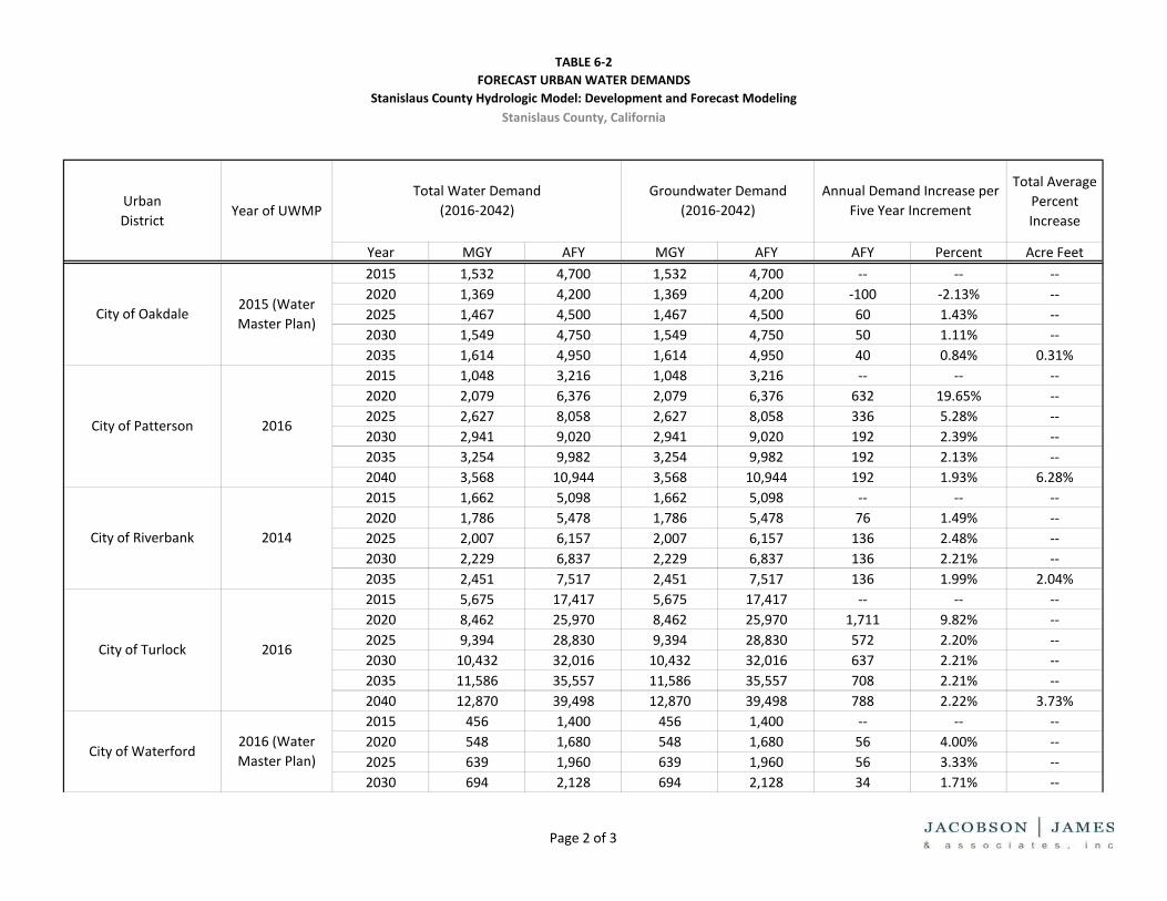
TABLE 6‐2FORECAST URBAN WATER DEMANDS
Stanislaus County Hydrologic Model: Development and Forecast ModelingStanislaus County, California
Total Average Percent Increase
Year MGY AFY MGY AFY AFY Percent Acre Feet
Annual Demand Increase per Five Year IncrementYear of UWMP
Total Water Demand(2016‐2042)
Groundwater Demand(2016‐2042)Urban
District
2015 1,532 4,700 1,532 4,700 ‐‐ ‐‐ ‐‐2020 1,369 4,200 1,369 4,200 ‐100 ‐2.13% ‐‐2025 1,467 4,500 1,467 4,500 60 1.43% ‐‐2030 1,549 4,750 1,549 4,750 50 1.11% ‐‐2035 1,614 4,950 1,614 4,950 40 0.84% 0.31%2015 1,048 3,216 1,048 3,216 ‐‐ ‐‐ ‐‐2020 2,079 6,376 2,079 6,376 632 19.65% ‐‐2025 2,627 8,058 2,627 8,058 336 5.28% ‐‐2030 2,941 9,020 2,941 9,020 192 2.39% ‐‐2035 3,254 9,982 3,254 9,982 192 2.13% ‐‐2040 3,568 10,944 3,568 10,944 192 1.93% 6.28%2015 1,662 5,098 1,662 5,098 ‐‐ ‐‐ ‐‐2020 1,786 5,478 1,786 5,478 76 1.49% ‐‐2025 2,007 6,157 2,007 6,157 136 2.48% ‐‐2030 2,229 6,837 2,229 6,837 136 2.21% ‐‐2035 2,451 7,517 2,451 7,517 136 1.99% 2.04%2015 5,675 17,417 5,675 17,417 ‐‐ ‐‐ ‐‐2020 8,462 25,970 8,462 25,970 1,711 9.82% ‐‐2025 9,394 28,830 9,394 28,830 572 2.20% ‐‐2030 10,432 32,016 10,432 32,016 637 2.21% ‐‐2035 11,586 35,557 11,586 35,557 708 2.21% ‐‐2040 12,870 39,498 12,870 39,498 788 2.22% 3.73%2015 456 1,400 456 1,400 ‐‐ ‐‐ ‐‐2020 548 1,680 548 1,680 56 4.00% ‐‐2025 639 1,960 639 1,960 56 3.33% ‐‐2030 694 2,128 694 2,128 34 1.71% ‐‐
2016City of Turlock
2016City of Patterson
City of Oakdale
City of Waterford2016 (Water Master Plan)
2014City of Riverbank
2015 (Water Master Plan)
Page 2 of 3

TABLE 6‐2FORECAST URBAN WATER DEMANDS
Stanislaus County Hydrologic Model: Development and Forecast ModelingStanislaus County, California
Total Average Percent Increase
Year MGY AFY MGY AFY AFY Percent Acre Feet
Annual Demand Increase per Five Year IncrementYear of UWMP
Total Water Demand(2016‐2042)
Groundwater Demand(2016‐2042)Urban
District
2035 767 2,352 767 2,352 45 2.11% ‐‐2040 840 2,576 840 2,576 45 1.90% 2.61%
2.64%2.70%
Notes:AFY = acre foot per yearMGY = million gsllon per yearUWMP = Urban Water Management Plan% = percent
AverageMedian Average
City of Waterford(continued)
2016 (Water Master Plan)
Page 3 of 3

TABLE 6‐3FORECAST SCENARIO GROUNDWATER BUDGET COMPARISON
Stanislaus County Hydrologic Model: Development and Forecast ModelingStanislaus County, California
Scenario 2 Scenario 3 Scenario 4a Scenario 4b Scenario 5 Scenario 2 Scenario 3 Scenario 4a Scenario 4b Scenario 5Change in Stream Gain
from GW (AC‐FT)72 39 (3,390) (1,525) 86 682 174 (3,964) (1,948) 1,528
Cumulative Storage Change (AC‐FT)
(7,612) (1,044) (135,676) (138,058) (7,057) (35,935) (4,967) (155,574) (171,005) (12,131)
Annual Storage Change (AC‐FT)
(63) (7) (837) (1,031) 95 (479) (52) 29 52 (469)
Change in Stream Gain from GW (AC‐FT)
(2,809) (556) (1,419) (1,714) (2,799) (18,649) (3,519) (2,923) (3,182) (18,428)
Cumulative Storage Change (AC‐FT)
(255,244) (48,244) (175,725) (162,065) (255,201) (3,433,006) (627,837) (636,517) (549,882) (3,430,237)
Annual Storage Change (AC‐FT)
(5,600) (1,021) (2,861) (2,417) (5,591) (21,772) (4,005) (1,306) (1,115) (21,766)
Change in Stream Gain from GW (AC‐FT)
(9,413) (1,851) (8,963) (7,163) (6,714) (57,614) (10,973) (13,068) (11,411) (48,206)
Cumulative Storage Change (AC‐FT)
(337,180) (64,877) (266,959) (273,856) (334,436) (2,952,544) (562,514) (644,028) (654,576) (2,905,847)
Annual Storage Change (AC‐FT)
(6,690) (1,277) (4,420) (4,597) (6,203) (17,992) (3,422) (268) (245) (17,970)
Change in Stream Gain from GW (AC‐FT)
(5,057) (924) (2,853) (2,434) (5,027) (26,372) (4,982) (3,066) (2,782) (23,579)
Cumulative Storage Change (AC‐FT)
(331,978) (62,373) (315,628) (340,189) (257,691) (2,217,507) (425,147) (363,417) (417,594) (1,191,660)
Annual Storage Change (AC‐FT)
(4,678) (947) (853) (1,407) 8,202 (11,682) (2,346) (50) (64) (10,887)
Notes:AC‐FT = acre feetGW = groundwaterWY = water year
Modesto
Turlock
Groundwater Budget Change Relative to Baseline in WY 2022 Groundwater Budget Change Relative to Baseline in WY 2042
Delta‐Mendota
Eastern San Joaquin
Water Budget Component
Subbasin
Page 1 of 1

Model Year (1990 – 2042)
Hydrology Data Year
Data Year Unimpaired Runoff in San Joaquin
Valley (MAF)
Data Year Type
Climate Adjustment 2016 ‐ 2042
(Temperature ᵒC)
1990 1990 2.46 C ‐‐1991 1991 3.2 C ‐‐1992 1992 2.58 C ‐‐1993 1993 8.38 W ‐‐1994 1994 2.54 C ‐‐1995 1995 12.32 W ‐‐1996 1996 7.22 W ‐‐1997 1997 9.51 W ‐‐1998 1998 10.43 W ‐‐1999 1999 5.91 AN ‐‐2000 2000 5.9 AN ‐‐2001 2001 3.18 D ‐‐2002 2002 4.06 D ‐‐2003 2003 4.87 BN ‐‐2004 2004 3.81 D ‐‐2005 2005 9.21 W ‐‐2006 2006 10.44 W ‐‐2007 2007 2.51 C ‐‐2008 2008 3.49 C ‐‐2009 2009 4.94 BN ‐‐2010 2010 6.08 AN ‐‐2011 2011 10.99 W ‐‐2012 2012 2.76 D ‐‐2013 2013 3.05 C ‐‐2014 2014 1.72 C ‐‐2015 2015 1.44 C ‐‐2016 2000 5.9 AN 0.03552017 1983 15.01 W 0.07102018 1984 7.13 AN 0.10652019 1985 3.6 D 0.14202020 1986 9.5 W 0.17752021 1987 2.08 C 0.21302022 1995 12.32 W 0.24852023 1996 7.22 W 0.28402024 1997 9.51 W 0.31952025 1998 10.43 W 0.35502026 1999 5.91 AN 0.39052027 2003 4.87 BN 0.42602028 2004 3.81 D 0.46152029 2005 9.21 W 0.49702030 2006 10.44 W 0.53252031 2007 2.51 C 0.56802032 2008 3.49 C 0.60352033 2009 4.94 BN 0.63902034 2010 6.08 AN 0.67452035 2011 10.99 W 0.71002036 2012 2.76 D 0.74552037 2013 3.05 C 0.78102038 2014 1.72 C 0.81652039 2015 1.44 C 0.85202040 2000 5.9 AN 0.88752041 2001 3.18 D 0.92302042 2002 4.06 D 0.9585
Stanislaus County Hydrologic Model: Development and Forecasts
Stanislaus County, California
FIGURE 6-1
SCHM Forecast Hydrologic Data, 2016 - 2042
PROJECT NO.
STANCO.002
DATE
10/24/17
DRAWN BY
JH
APPR. BY
MT
Notes: Notes: AN = above normal BN = below normal C = critically dry D = dry MAF = million acre foot ᵒC = degree Celsius
Source: California Department of Water Resources, California Data Exchange Center. California Cooperative Snow Surveys. Website: http://cdec.water.ca.gov/cgi‐progs/iodir/WSIHIST.
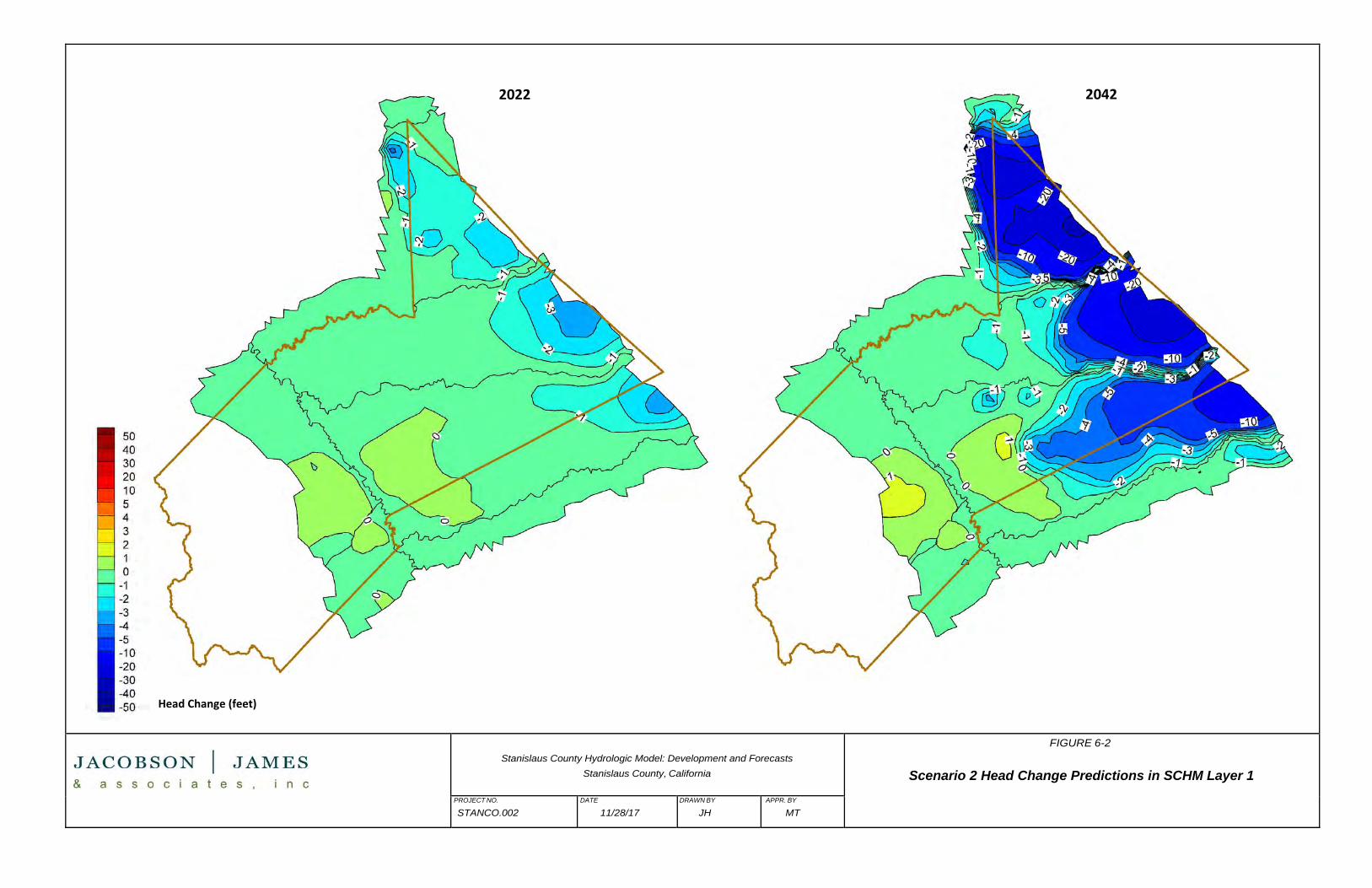
Stanislaus County Hydrologic Model: Development and Forecasts
Stanislaus County, California
FIGURE 6-2
Scenario 2 Head Change Predictions in SCHM Layer 1
PROJECT NO.
STANCO.002
DATE
11/28/17
DRAWN BY
JH
APPR. BY
MT
2022
Head Change (feet)
2042

Stanislaus County Hydrologic Model: Development and Forecasts
Stanislaus County, California
FIGURE 6-3
Scenario 2 Head Change Predictions in SCHM Layer 2
PROJECT NO.
STANCO.002
DATE
11/28/17
DRAWN BY
JH
APPR. BY
MT
2022
Head Change (feet)
2042

Stanislaus County Hydrologic Model: Development and Forecasts
Stanislaus County, California
FIGURE 6-4
Scenario 3 Head Change Predictions for SCHM Layer 1
PROJECT NO.
STANCO.002
DATE
11/28/17
DRAWN BY
JH
APPR. BY
MT
2022
Head Change (feet)
2042
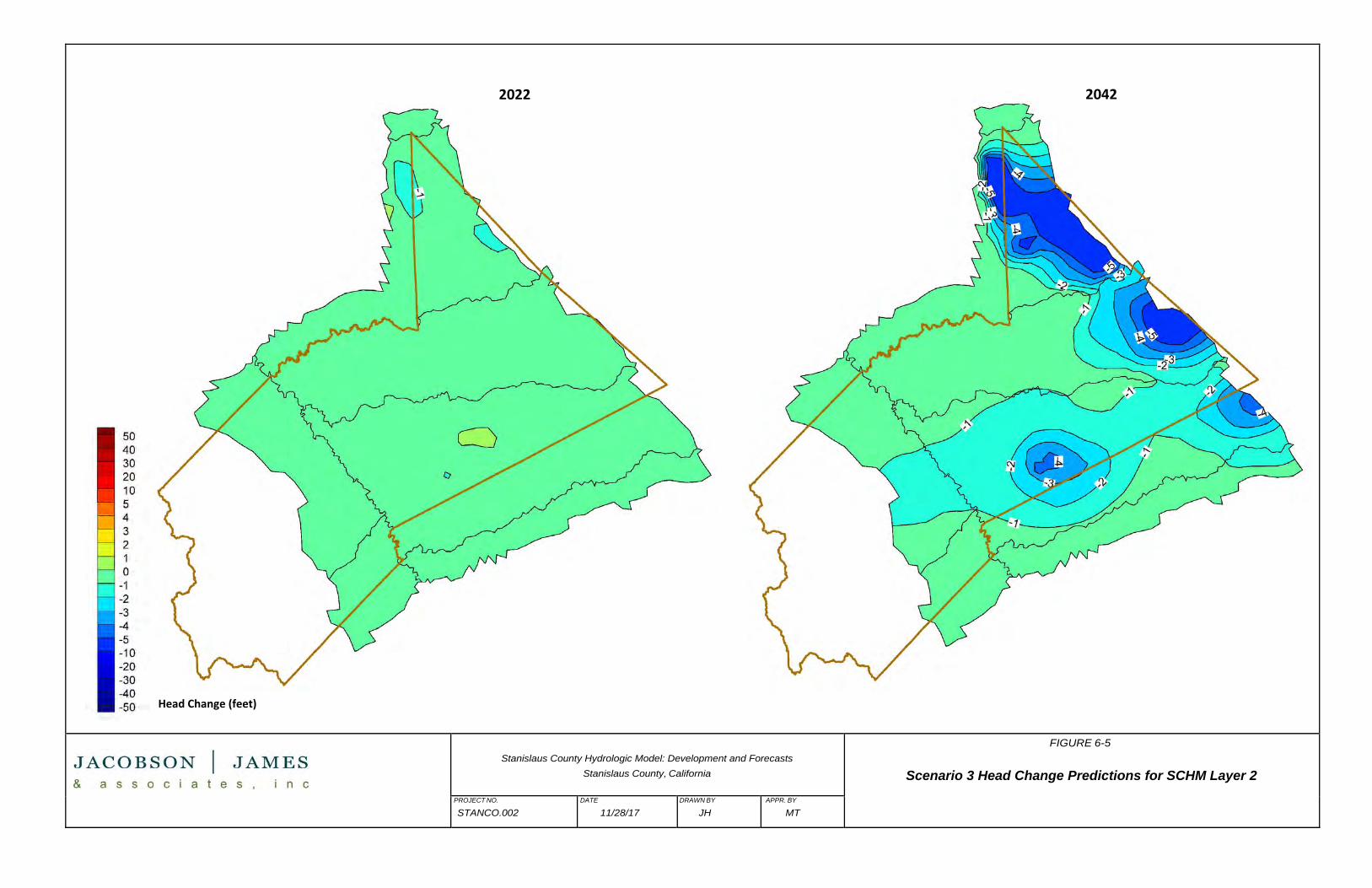
Stanislaus County Hydrologic Model: Development and Forecasts
Stanislaus County, California
FIGURE 6-5
Scenario 3 Head Change Predictions for SCHM Layer 2
PROJECT NO.
STANCO.002
DATE
11/28/17
DRAWN BY
JH
APPR. BY
MT
2022
Head Change (feet)
2042

Stanislaus County Hydrologic Model: Development and Forecasts
Stanislaus County, California
FIGURE 6-6
Scenario 4a and 4b:
Location of Simulated Wells and Year Installed PROJECT NO.
STANCO.002
DATE
11/28/17
DRAWN BY
JH
APPR. BY
MT
Stanislaus County Hydrologic Model Finite Element Mesh General Head Boundary No Flow Boundary Stanislaus County Boundary MERSTAN (Merced‐Stanislaus) Model Boundary Simulated Wells with Year Installed

Stanislaus County Hydrologic Model: Development and Forecasts
Stanislaus County, California
FIGURE 6-7
Scenario 4a Head Change Predictions for SCHM Layer 1
PROJECT NO.
STANCO.002
DATE
11/28/17
DRAWN BY
JH
APPR. BY
MT
2022
Head Change (feet)
2042

Stanislaus County Hydrologic Model: Development and Forecasts
Stanislaus County, California
FIGURE 6-8
Scenario 4a Head Change Predictions for SCHM Layer 2
PROJECT NO.
STANCO.002
DATE
11/28/17
DRAWN BY
JH
APPR. BY
MT
2022
Head Change (feet)
2042
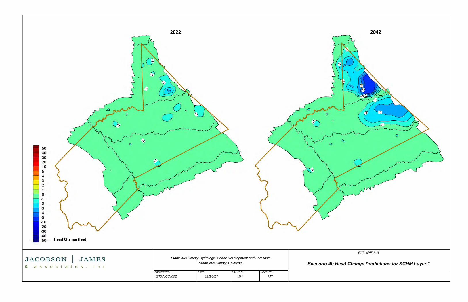
Stanislaus County Hydrologic Model: Development and Forecasts
Stanislaus County, California
FIGURE 6-9
Scenario 4b Head Change Predictions for SCHM Layer 1
PROJECT NO.
STANCO.002
DATE
11/28/17
DRAWN BY
JH
APPR. BY
MT
2022
Head Change (feet)
2042

Stanislaus County Hydrologic Model: Development and Forecasts
Stanislaus County, California
FIGURE 6-10
Scenario 4b Head Change Predictions for SCHM Layer 2
PROJECT NO.
STANCO.002
DATE
11/28/17
DRAWN BY
JH
APPR. BY
MT
2022
Head Change (feet)
2042

Stanislaus County Hydrologic Model: Development and Forecasts
Stanislaus County, California
FIGURE 6-11
Scenario 5 Head Change Predictions for SCHM Layer 1
PROJECT NO.
STANCO.002
DATE
11/28/17
DRAWN BY
JH
APPR. BY
MT
2022
Head Change (feet)
2042

Stanislaus County Hydrologic Model: Development and Forecasts
Stanislaus County, California
FIGURE 6-12
Scenario 5 Head Change Predictions for SCHM Layer 2
PROJECT NO.
STANCO.002
DATE
11/28/17
DRAWN BY
JH
APPR. BY
MT
2022
Head Change (feet)
2042

Stanislaus County Hydrologic Model: Development and Forecasts December 20, 2017
Page 7-1
7.0 CONCLUSIONS AND RECOMMENDATIONS
The primary objectives of developing the SCHM were to provide a tool that may be used for evaluation of
program-level impacts of implementing the County’s discretionary well permitting program, and producing
an incremental improvement in understanding and modeling of regional hydrogeologic conditions that builds
on past efforts and can help inform future studies leading up to development of GSPs. The groundwater
budget, cross boundary flow, and some head data produced by the SCHM should be considered preliminary
and indicative; however, the forecast data are produced using a superposition approach that is adequate for
the evaluation of program-level impacts to groundwater resources. As noted in the preceding sections,
further refinement of groundwater modeling in the area will be needed to produce subbasin-scale models
that can support the preparation of GSPs, or that are suitable for evaluation of groundwater and other
hydrologic impacts associated with specific projects. This can be accomplished through the construction of
new models, by updating the SCHM, or by creating more detailed “child” models within the SCHM domain
that incorporate sufficient refinements to meet future modeling objectives. The construction, calibration and
sensitivity testing of the SCHM, as well as its use to evaluate historical conditions and forecast future
conditions, provides key information to identify and prioritize data needs and opportunities to support such
activities. Key findings and recommendations are discussed below.
7.1 Principal Findings of Forecast Analysis
The modeling forecast analysis provided insights into changes in water budgets and groundwater levels that
could occur throughout the County under a variety of scenarios and stresses. Both water budgets and
groundwater levels are discussed in Section 6 and principal findings are summarized below. Table 7-1
provides a summary of the model forecast water budgets for the entire model area.
Table 7-1a Modeling Forecast Water Budget Summary
Combined All Subbasins
Groundwater Budget Change Relative to Baseline in WY 2022
Scenario 2 Upper Bound
Demand Increase
Scenario 3 Lower Bound
Demand Increase
Scenario 4a Discretionary
Well Permitting Shallow Aquifer
Scenario 4b Discretionary
Well Permitting
Deep Aquifer
Scenario 5 Additional
Surface Water
Delivery
Change in Stream Gain from GW (AC-FT)
(17,207) (3,292) (16,625) (12,835) (14,454)
Cumulative Storage Change (AC-FT)
(932,014) (176,538) (893,987) (914,168) (854,385)
Annual Storage Change (AC-FT)
(17,031) (3,252) (8,972) (9,452) (3,498)

Stanislaus County Hydrologic Model: Development and Forecasts December 20, 2017
Page 7-2
Table 7-1b Modeling Forecast Water Budget Summary
Combined All Sub-Basins
Groundwater Budget Change Relative to Baseline in WY 2042
Scenario 2 Upper Bound
Demand Increase
Scenario 3 Lower Bound
Demand Increase
Scenario 4a Discretionary
Well Permitting Shallow Aquifer
Scenario 4b Discretionary
Well Permitting
Deep Aquifer
Scenario 5 Additional
Surface Water
Delivery
Change in Stream Gain from GW (AC-FT)
(101,954) (19,299) (23,021) (19,323) (88,685)
Cumulative Storage Change (AC-FT)
(8,638,993) (1,620,466) (1,799,536) (1,793,056) (7,539,876)
Annual Storage Change (AC-FT)
(51,925) (9,825) (1,595) (1,372) (51,091)
Principal conclusions from the SCHM forecast analysis include the following.
• Comparing water budgets over the short term (Table 7-1a through WY 2022), the reasonable lower
bound demand increase scenario (Scenario 3) results in the least stream depletion and removes the
least water from storage (cumulative and annual). Over the long term (Table 7-1b through WY 2042),
decreased demand and the discretionary well permitting program (with wells in either the shallow
aquifer [Scenario 4a] or deep aquifer [Scenario 4b] zones), water budget are similar and have
significantly less impacts to stream depletion and groundwater storage compared to Scenario 2 (the
reasonable upper bound demand increase scenario. The difference in streamflow and aquifer
depletion simulated in Scenario 5 (additional surface water) decreases the effects of Scenario 2, and
would compensate for a large percentage of Scenario 3 impacts.
• In all of the forecast scenarios except Scenario 4b (discretionary well permitting with addition of new
wells in the deeper aquifer), increases in groundwater demand led to a greater drawdown response
in the eastern foothills area of the model than in other locations. This was generally true in both
Model Layer 1 and 2 (the shallow aquifer system and the deeper aquifer system), and appears to
reflect a greater relative sensitivity of this area to groundwater stresses. Greater sensitivity to
drawdown stresses in this area may result from less local recharge being available due to local soil
conditions and a lack of surface water availability.
• A second area of the model where groundwater stresses appeared to result in greater drawdown is
the north central area of the model in Model Layer 2 beneath the Corcoran Clay. This area displayed
the greatest amount of drawdown in Scenario 4b, which evaluated the effects of permitting
discretionary wells in the deeper aquifer. The area may be more susceptible to drawdown because
it represents a terminal outflow point of the model, where water budget effects become cumulative,
and because the strongly confined nature of the deeper aquifer system beneath the Corcoran Clay

Stanislaus County Hydrologic Model: Development and Forecasts December 20, 2017
Page 7-3
results in greater drawdown per unit volume of water extracted. The historical model simulates a
broad cone of depression in this area (Figures 4-7 and 4-8), as does C2VSim.
• Groundwater extraction in the western portion of the model and from the shallow aquifer system
resulted in higher amounts of streamflow depletion than groundwater withdrawal from the deeper
aquifer or in other areas. Nevertheless, the increases in streamflow depletion resulting from higher
groundwater demand were relatively modest, and the amount of total streamflow depletion that
was forecast was relatively modest and below the typical range of error of stream gaging stations
(typically about +/- 5 %).
• Groundwater level drawdown from municipal pumping was greatest in cities that rely primarily on
wells completed in the deeper aquifer system, such as Turlock. Increase in municipal demand in
these areas were accompanied by a slight increase in shallow groundwater levels resulting from deep
percolation of return flows, while groundwater extraction from the confined, deep aquifer system
led to higher rates of drawdown than in other areas.
• The greatest amount of drawdown was predicted under Scenario 2 (reasonable upper bound
potential demand increase), which is based on worst case assumptions regarding municipal, rural
domestic and agricultural demand growth. Demand growth at the simulated rates has a low
likelihood of ever being realized, but coupled with Scenario 3 (reasonable lower bound potential
demand increase), which incorporates a more realistic demand growth scenario, provides a useful
preliminary perspective for investigating the relationship between demand growth, drawdown, and
sustainable yield.
• Scenario 5 (Scenario 2 with additional surface water delivery) illustrates the effectiveness of
conjunctive use projects to help alleviate local drawdown. For perspective, the surface water supply
rates simulated in this scenario appear capable of moderating the drawdown resulting from worst
case demand growth (Scenario 2), and more than offset the drawdown associated with a more
reasonable demand growth rate (Scenario 3). However, the volumes of surface water assumed to
be supplied under Scenario 5 are relatively small compared to regional demand, and did little to
offset streamflow or storage depletion at a subbasin level.
7.2 Principal Findings and Recommendations from Model Construction and
Calibration
7.2.1 Selected Model Code and Scheduled Improvements
Updates to the DWR’s C2VSim are being developed using the IWFM 2015 modeling code, which features an
improved ability to apply water budget data, simulate demand, route deep percolation, and other
key features. The USGS is also working to refine the CVHM and MERSTAN models. In addition, efforts are
underway to develop improved cropping and evapotranspiration datasets. These efforts, which were in
progress as the SCHM was being developed, will be available for use by future subbasin-scale modeling efforts

Stanislaus County Hydrologic Model: Development and Forecasts December 20, 2017
Page 7-4
needed to support GSP development. Finally, subbasin scale modeling efforts were in progress in the Eastern
San Joaquin Subbasin to the north and west of the SCHM domain, and to the south of the SCHM in the Merced
Subbasin. It is expected that the results of these efforts will be useful to better understanding water budget
processes in the region and cross boundary flows into and out of these respective modeling areas.
7.2.2 Water Budgets
Efforts during construction of the SCHM focused on refinement of water budgets to a greater degree than
refinement of model lithology or model calibration. Nevertheless, significant data needs and opportunities
for further refinement of local and regional water budgets remain that were beyond of the scope of the
current project to address. These include the following.
• Additional data likely exist regarding urban and agricultural water demand, well completions, surface
water deliveries, system losses, tile drainage, return flows and system “spill”, that were not provided
by water districts or available from published plans. These data could be used as an input to improve
understanding of regional, subbasin and local water budgets, and would serve as a primary data
source to help guide future model calibration and refinement efforts.
• Refined datasets regarding historical cropping patterns and evapotranspiration based on
improvements in remote sensing data application are being developed by DWR. As was stated in
Section 4.5.3, agricultural pumping accounts for 80 to 89% of groundwater pumping in the County.
Therefore, these data, coupled with comparison to data from the Agricultural Commissioner and
field-level verification, provide a significant and necessary opportunity for model refinement. As
illustrated by the results of the sensitivity analysis for evapotranspiration, accurate data regarding
these key agricultural water budget inputs are essential to model accuracy and to producing
meaningful calibration results. These data should be incorporated into future modeling efforts based
on codes (such as IWFM 2015) with an improved capability of applying and simulating agricultural
water budget processes.
• Urban water budgets in the SCHM were refined using updated historical demand data and well
completion information, but urban water budget processes in the SCHM are based largely on ad hoc
assumptions incorporated into the C2VSim that may be appropriate for regional modeling, but can
be substantially refined for more local application. This includes information regarding system
leakage, wastewater return flow, indoor vs. outdoor water use, storm drainage and urban
evapotranspiration, among others. Refinements to the processes are available in IWFM 2015, and
should be applied in tandem with investigation of refined urban water budgets.
• Industrial groundwater pumping data were not provided for the development of the SCHM. The
approach taken to developing rural domestic groundwater demand inputs for the SCHM around
urban fringes may compensate for this deficiency somewhat by estimating higher rural domestic
demand in areas where the model water budget subregions overlap with both urban and rural census
tracts. Industrial groundwater users in the region tend to be located in these urban fringe areas.

Stanislaus County Hydrologic Model: Development and Forecasts December 20, 2017
Page 7-5
However, the extent of this effect has not been evaluated. If provided in the future, industrial
groundwater demand data would be useful for developing a refined understanding of urban water
budgets.
• Recharge from offstream storage reservoirs in eastern Stanislaus County is an important water
budget component. C2VSim does not include these reservoirs, and recharge rates incorporated into
MERSTAN were based on rough estimates. Recharge rates were developed for SCHM based on
district-provided water balance data, but could likely be refined. A disparity existed between the
recharge rates estimated for Woodward and Modesto Reservoir, and those estimated based on data
provided for Turlock Lake, with the rates for Turlock Lake being several times higher even though the
reservoirs are all of fairly similar size and located in similar geologic settings. During the calibration
process, high water levels were noted in the vicinity of Turlock Lake and the recharge rate for this
lake was therefore adjusted downward. It would be desirable to further investigate the actual
recharge rates for these reservoirs, as the most complete water balance dataset among the three
reservoirs was provided for Turlock Lake, and this adjustment was not based on a comparison to the
other reservoir for which data was more limited, and local groundwater levels.
7.2.3 Measured and Simulated Groundwater Levels
Development of groundwater level calibration datasets and calibration of the SCHM revealed that the current
CASGEM dataset, which does not differentiate monitoring data from different hydrostratigraphic zones, may
lead to an overly simplified understanding of groundwater levels and flow. In many cases, we found that
wells completed to total depths within Model Layer 2 had measured water levels that were more consistent
with simulated and measured water levels in Model Layer 1. When considered together with data from other
nearby wells, in many cases it appeared that this was a function of the well construction rather than an
inaccuracy in the modeling results. Theoretically this is possible when deep wells cross-connect the upper
and lower aquifer systems mixing water from the two zones due to annular flow, cross screening or damaged
well casings, and vertical flow in the wells causes water levels within the well to be dominated by higher
groundwater levels in the upper aquifer system. Further work is warranted to investigate groundwater levels
in the shallow and confined aquifer systems, especially in the area underlain by the Corcoran Clay.
Historical groundwater level data in the eastern foothill region of the SCHM is, at present, relatively sparse,
but efforts are underway by Stanislaus County and the Agricultural Preservation Alliance (APA) to compile
additional data that can help inform future modeling efforts.
Based on the above observation and the simulate historical SCHM model results for Model Layer 1 and Model
Layer 2, groundwater levels in the confined aquifer system beneath the Corcoran Clay may be deeper than
has previously be recognized on a regional basis. However, the calibration data also indicate that the model
has a bias toward underpredicting water levels in Model Layer 2. Model Layer 2 beneath the Corcoran Clay
in the north-central portion of the County represents the most downgradient portion of the model domain,
and be subject to the cumulative effects of all upstream model inputs, including any errors. Investigation of

Stanislaus County Hydrologic Model: Development and Forecasts December 20, 2017
Page 7-6
groundwater levels at discrete hydrostratigraphic intervals will be key to making meaningful improvements
in model calibration and refining model accuracy.
7.2.4 Model Aquifer Parameters
The most sophisticated lithology dataset in the SCHM region stems from extensive work completed by the
USGS for the MERSTAN model. Care was taken during calibration of the SCHM not to disregard this dataset
and make widespread hydraulic conductivity adjustments in this area when other model inputs are not
constrained at a similar level of detail. Outside the active MERSTAN domain to the east and to the west, a
limited dataset of specific capacity and aquifer tests was utilized to update model hydraulic conductivity.
Additional specific capacity test data are being compiled by Stanislaus APA for the eastern foothills area of
the SCHM and will be available to help inform future modeling efforts. Similar data may be available for the
Delta-Mendota Subbasin portion of the SCHM. Alternatively, well log data for these areas could be compiled
and analyzed geostatistically to expand the MERSTAN geostatistical lithology model the edges of the
groundwater basin.
The model sensitivity analysis indicates that lateral hydraulic conductivity, vertical hydraulic conductivity, and
storage coefficients are all sensitive parameters, and the model could be improved through their refinement.
The greatest variation noted in the sensitivity analysis was in response due to decreases in lateral hydraulic
conductivity, which produced the greatest head decline below the Corcoran Clay in Layer 2, although Layer 1
was also sensitive to this parameter to a lesser degree. An unexpected result was the variation in effect from
one location to another, especially in Layer 1. The same change produced increases and declines in
groundwater levels in adjacent areas. The source of this variability should be further investigated in order to
facilitate future changes to the model inputs.
Aquifer storage coefficients had a more uniform effect on groundwater levels, which was most pronounced
in Layer 2. Relatively few data sources for aquifer storage coefficients exist within the SCHM domain.
Additional data from aquifer tests may exist that were not considered in constructing the SCHM, and deriving
additional data from future aquifer tests would help to constrain this important parameter and support more
refined and meaningful model calibration.
The vertical hydraulic conductivity of the Corcoran Clay is a key parameter in terms of its influence on
groundwater flow and levels, especially in Layer 2, yet little direct data exist to substantiate this property
within the SCHM domain. Focused studies to help constrain this property on a subregional basis, laboratory
analysis of cores, and/or carefully constructed aquifer testing would help to constrain this parameter and
support more refined and meaningful model calibration.

Stanislaus County Hydrologic Model: Development and Forecasts December 20, 2017
Page 8-1
8.0 REFERENCES
Aquacraft, 2011. California Single Family Water Use Efficiency Study. June.
Anderson, Mary P. and Woessner, W.W., 2002. Applied Groundwater Modeling, Simulation of Flow and Advective Transport. Academic Press.
Daly et al. 1997. The Prism Approach to Mapping Precipitation and Temperature.
Daly, C., Gibson, W.P., Doggett, M., Smith, J. and Taylor, G., 2004. Up-to-date monthly climate maps for the conterminous United States. In Proc., 14th AMS Conf. on Applied Climatology, 84th AMS Annual Meeting Combined Preprints, Amer. Meteorological Soc., Seattle, WA. January.
California Department of Water Resources (DWR), 2013a. California’s Groundwater Update 2013, A Compilation of Enhanced Content for California Water Plan Update 2013, Chapter 8 – San Joaquin River Hydrologic Region. April.
DWR, 2013b. Development and Calibration the California Central Valley Groundwater-. Surface Water Simulation Model (C2VSim), Version 3.02-CG. DWR Technical Memorandum. June.
DWR, 2013c. Integrated Water Flow Model Version 3.02, Theoretical Documentation. October.
DWR, 2015a. Draft List of Critically Overdrafted Basins – August 6, 2015. August.
DWR, 2015b. Groundwater Information Center Interactive Mapping Application. Website: https://gis.water.ca.gov/app/gicima/. Last edited January 15, 2015. Accessed December, 2015.
DWR, 2016a. C2VSim: California Central Valley Groundwater-Surface Water Simulation Model. Website: http://baydeltaoffice.water.ca.gov/modeling/hydrology/C2VSim/index_C2VSIM.cfm
DWR, 2016b. Best Management Practices for the Sustainable Management of Groundwater: Modeling. December.
DWR, 2017a. California Data Exchange Center. Website: http://cdec.water.ca.gov/cgi-progs/iodir/WSIHIST
DWR, 2017b. Groundwater Information Center Interactive Map Application. Website: https://gis.water.ca.gov/app/gicima/
Cordero, E.C., Kessomkiat, W., Abatzoglou, J. and Mauget, S.A., 2011. The identification of distinct patterns in California temperature trends. Climatic change, 108(1), pp.357-382.
Davids Engineering, 2015. 2015 Agricultural Water Management Plan, South San Joaquin Irrigation District. December.
Durbin, 2008. Assessment of Future Groundwater Impacts due to Assumed Water-Use Changes, Turlock Groundwater Basin, California. Prepared for the Turlock Groundwater Basin Association, September.
Jacobson James & Associates, Inc. (JJ&A), 2016a. Groundwater Resources Impact Assessment, Crows Landing Industrial Business Park, Stanislaus County, California. Prepared for Stanislaus County Division of Public Works. October.
JJ&A, 2016b. Hydrologic Modeling Plan, Program Environmental Impact Report for Implementation of the Stanislaus County Groundwater Ordinance. December.
Stanislaus County Hydrologic Model: Development and Forecasts December 20, 2017
Page 8-2
JJ&A, 2017. Draft Initial Study and Mitigated Negative Declaration, Well Permit Application 2017-117, Larry Gillum, Stanislaus County, California. Prepared for Stanislaus County Department of Environmental Resources. October.
Makkink, G.F. 1957. Testing the Penman formula by means of lysimeters. J. Inst. of Water Eng. 11: 277-288.
Michael Baker International, 2016. Stanislaus County 2015 – 2023 Housing Element Update. April.
Phillips, S.P., Rewis, D.L., and Traum, J.A., 2015. Hydrologic model of the Modesto Region, California, 1960–2004. U.S. Geological Survey Scientific Investigations Report, 2015–5045, 69 p. Website:.
Reilly, Thomas E., Franke, O. Lehn, and Bennett, Gordon D., 1987. The Principle of Superposition and its
Application in Ground-Water Hydraulics. U.S. Geological Survey Techniques of Water-Resources
Investigations 03-B6.
State Water Resources Control Board (SWRCB), 2012. Draft Substitute Environmental Document in Support of Potential Changes to the Water Quality Control Plan for the Bay-Delta: San Joaquin River Flows and Southern Delta Water Quality. December.
SWRCB, 2015. A Guide for Private Domestic Well Owners. Website: http://www.waterboards.ca.gov/gama/docs/wellowner_guide.pdf. Accessed September 14, 2016.
SWRCB, 2016. Draft Revised Substitute Environmental Document in Support of Potential Changes to the Water Quality Control Plan for the Bay-Delta: San Joaquin River Flows and Southern Delta Water Quality. September 15.
San Luis & Delta Mendota Water Use Authority (SLDMWUA), 2011. Groundwater Management Plan for the Northern Agencies in the Delta Mendota Canal Service Area. November.
Todd Groundwater and RMC Groundwater and Environment (Todd and RMC), 2016. Groundwater Characterization and Recharge Study, Modesto LGA Project. Prepared for the City of Modesto. June.
Turlock Groundwater Basin Association (TGBA), 2008. Turlock Groundwater Basin Groundwater Management Plan. March.
United States Geological Survey (USGS), 2004a. Guidelines for Evaluating Ground-Water Flow Models. Scientific Investigations Report 2004-5038.
USGS, 2004b. Hydrogeologic Characterization of the Modesto Area, San Joaquin Valley, California. Scientific Investigations Report 2004-5232.
USGS, 2009. Groundwater Availability of the Central Valley Aquifer. California: U.S. Geological Survey Professional Paper 1766.
USGS, 2012. Extent of Corcoran Clay modified from Page (1986) for the Central Valley Hydrologic Model (CVHM). USGS Professional Paper 1766. Accessed at https://water.usgs.gov/GIS/metadata/usgswrd/XML/pp1766_corcoran_clay_extent.xml
USGS, 2015. Hydrologic Model of the Modesto Region, California, 1960-2004. Scientific Investigations Report
2015-5045.
USGS, 2017. Central Valley Hydrologic Model (CVHM). Website: http://ca.water.usgs.gov/projects/central-
valley/central-valley-hydrologic-model.html

Stanislaus County Hydrologic Model: Development and Forecasts December 20, 2017
Page 8-3
West Yost, 2016. Preliminary Phasing and Water Treatment Plant Sizing for the SRWA Surface Water Supply
Project. June 16..
West Yost, 2017. Surface Water Supply Project, Initial Project Capacity, Estimated Cost and Rate Impacts.
Presentation to Stanislaus Regional Water Authority. August 3.
Water Research Foundation, 2016. Residential End Uses of Water, Version 2. April.
Woodard, Gary, 2015. The Surprising Slide in Domestic Demand: Be Careful What You Wish For. Presentation
at the Water Resources Research Center (WRRC), University of Arizona. March.
APPENDIX A
DATA REGARDING CONVERSION OF NON-DISTRICT RANGELAND IN EASTERN STANISLAUS
COUNTY TO PERMANENT CROPS FROM 2000 TO 2015

MID
EAST SIDEWD
TID
OID
TUOLUMNE RIVER
DRY CREEK
STANISLAUS RIVER
Simmon Creek
Wood Chopper Gulch
Rock
Cre
ek
Little John Creek
S mith Cree k
Hoods Creek
Simm
onsCree
k
Hood Creek
Lone Tree Creek
Duck Creek
Hoods Creek
Sh
irle
yC
ree
k
Dry Creek
2001 2005/2006
OID
MID
TID EAST SIDE WD
TUOLUMNE RIVER
DRY CREEK
STANISLAUS RIVER
Simmon Creek
Wood Chopper Gulch
Ro
ckC
reek
Little John Creek
S mith Cree k
Hoods Creek
Duck
Creek
Simm
onsCre
ek
Hood Creek
Lone Tree Creek
Hoods Creek
Shir
ley
Creek
Dry Creek
LegendCOMMODITY
Almond-1,659 ac.
Grapes-28 ac
Walnuts-387 ac.
TID
OakdWD
MID
EastSideWD
River
Creek
County Boundary
LegendCOMMODITY
Almond-11,519 ac.
Grapes-1,340 ac
Walnuts-2,665 ac.
TID
OakdWD
MID
EastSideWD
River
Creek
County Boundary
DRAFT Copy
Stanislaus County shall assume no liability for:1.Any errors, omissions, or inaccuracies in the information provided regardless of how caused; or2.Any decision made or action taken or not taken by the reader in reliance upon any information or data furnished hereunder.
Stanislaus County shall assume no liability for:1.Any errors, omissions, or inaccuracies in the information provided regardless of how caused; or2.Any decision made or action taken or not taken by the reader in reliance upon any information or data furnished hereunder.
2015
Docum
ent P
ath
: G
:\A
_S
ueB
\DE
R_
Pro
jects
\20
17\w
alt\C
rop
sO
uts
ide
WD
_U
pd08
201
4_0
320
17.m
xd
OID
MID
TID
EASTSIDEWD
Stanislaus County shall assume no liability for:1.Any errors, omissions, or inaccuracies in the information provided regardless of how caused; or2.Any decision made or action taken or not taken by the reader in reliance upon any information or data furnished hereunder.
LegendCOMMODITY
Almond-36,823 ac.
Grapes-3,758 ac
Walnuts-5,486 ac.
TID
OakdWD
MID
EastSideWD
River
Creek
County Boundary
2010
EAST SIDE WD
TID
MID
OID
DRAFT Copy
Stanislaus County shall assume no liability for:1.Any errors, omissions, or inaccuracies in the information provided regardless of how caused; or2.Any decision made or action taken or not taken by the reader in reliance upon any information or data furnished hereunder.
LegendCOMMODITY
Almond-16,548 ac.
Grapes-3,091 ac
Walnuts-3,832 ac.
TID
OakdWD
MID
EastSideWD
River
Creek
County Boundary