Technical Briefs - unipr.it · PDF fileTechnical Briefs An Inﬁnite ... Mechanical...

Journal ofDynamic Systems,

Measurement,and

ControlTechnical Briefs

t

a

vbir

i

r

n

h

ohr

to

ave

s

sign.entthe

thecu-st-this

ialre-lex-of

d tosult-

rs isig-

r

ort-trib-nsed

th

lern.

armghia-ple-taler

iblee

ac--

an-asere-lerble

s

An Infinite Dimensional DistributedBase Controller for Regulationof Flexible Robot Arms

Nader JaliliAssociate Mem. ASMEAssistant Professor,Robotics and Mechatronics Laboratory, Department ofMechanical Engineering, Clemson University,Clemson, SC 29634-0921e-mail: [email protected].

An exponentially stable variable structure controller is presenfor regulation of the angular displacement of a one-link flexibrobot arm, while simultaneously stabilizing vibration transientthe arm. By properly selecting the sliding hyperplane, the goveing equations which form a nonhomogenous boundary vaproblem are converted to homogenous ones, and hence, ancally solvable. The controller is then designed based on the ornal infinite dimensional distributed system which, in turn, remosome disadvantages associated with the truncated-model-controllers. Utilizing only the arm base angular position and tdeflection measurements, an on-line perturbation estimationtine is introduced to overcome the measurement imperfectionsever-present unmodeled dynamics. Depending on the composof the controller, some favorable features appear such as elimtion of control spillovers, controller convergence at finite timsuppression of residual oscillations and simplicity of the contimplementation. Numerical simulations along with experimenresults are provided to demonstrate and validate the effectiveof the proposed controller.@DOI: 10.1115/1.1408608#

1 IntroductionIn recent years, the demands for high-speed performance,

energy consumption and low cost have been motivating the uslightweight robot manipulators in industrial applications. Trigid structure of current industrial manipulators has made copliance impossible and limited the robotics use in automattasks. The use of lightweight flexible links, however, has led tchallenging problem in end-point trajectory control. Due to tflexibility distributed along the robot arms, an improved contscheme is required to track the desired trajectory while simuneously suppressing the vibrational transients in the arm.

This control problem has attracted significant attention inliterature. A flexible manipulator control must achieve the moti

Contributed by the Dynamic Systems and Control Division of THE AMERICANSOCIETY OF MECHANICAL ENGINEERS. Manuscript Received by the DynamicSystems and Control Division March 27, 2000. Associate Editor: C. Rahn.

712 Õ Vol. 123, DECEMBER 2001 Copyright

edleinrn-luelyti-

igi-esasepou-anditionna-e,oltaless

lowe ofem-ion

ae

ollta-

hen

tracking objectives~similar to that of rigid one! while stabilizingthe transient vibrations in the arm. Several control methods hbeen developed for flexible arms: optimal control@1,2#; finite el-ement approach@3,4#; model reference adaptive control@5#; adap-tive non-linear boundary control@6#; and several other techniqueincluding variable structure control~VSC! methods@7–9#. Mostof these methods concentrate on model-based controllers deSome of these controllers, however, may not be easy to implemdue to the uncertainties in the design model, large variations ofloads, ignored high frequency dynamics and high order ofdesigned controllers. In view of these methods, VSC is partilarly attractive due to its simplicity of implementation and robuness to parameter uncertainties. Successful applications ofmethod in practical systems are numerous~@10–12# are just afew!.

Generally, a flexible robot is governed by partial differentequations~PDE! as a system of distributed-parameter and thefore possesses infinite number of dimensions. Due to the compity of these equations and in order to facilitate the applicationcontrol strategies, discretization techniques are typically useconstruct a finite-dimensional reduced model. Based on the reing approximate model~assumed mode model~AMM ! or finiteelement method~FEM!, for instance! several controller designapproaches are then applied@4,5#, and@13#.

The problem associated with these model-based controllethe truncation procedure used in the approximation. Due tonored high frequency dynamics~related to control spillovers! andhigh order of the designed controller~related to increased numbeof flexible modes utilized in the model!, severe limitations occurin implementation of these controllers. To overcome these shfalls, alternative approaches based on infinite dimensional disuted ~IDD! partial differential models of flexible arms have beedeveloped. A direct strain feedback control strategy was propoto control vibration of flexible arm@9#, while an exponentiallystable VSC controller is utilized for flexible robot systems witranslational base@14#.

A common difficulty appears in all these IDD-base controldesign, which is the complexity of the control implementatioFor instance, the control strategy developed in@14# requires mea-surements of displacement, velocity and acceleration of thetip as well as the shear force at the root end of the link. Althouthe VSC controller is inherently insensitive to parameter vartions, feasible measurements are required for a successful immentation of the controller. This is the reason why experimenverification of these algorithms is progressing with a much slowpace than the theoretical compartment. For more complex flexsystems~multi-link arms, for instance! these approaches becomvery hard in practical implementation.

It is, therefore, highly desirable to seek a simple and yet prtical technique for control of flexible arms. To this end, an improved IDD-base controller is proposed to eliminate the disadvtages associated with the traditional truncated-model-bcontrollers. It is specifically intended to further relax the measument requirements for the flexible arm and simplify the controldesign. Only the tip deflection and angular position of the flexi

© 2001 by ASME Transactions of the ASME

nt

evru

tts

e

te,s-eirnous

ent

eearr-e

iatedthe

theme

ichith

zedatous-ire-of

le

the

arm are required to develop the new controller proposed here.remaining measurements, the ever-present unmodeled dynaand other parameter uncertainties are all combined to a siterm and estimated through an on-line perturbation estimaprocess@15,16#. This additional perturbation estimation will compromise the robustness and trajectory tracking accuracy.

2 Mathematical ModelingWe consider regulation of the angular displacement of a o

link flexible arm. As shown in Fig. 1, one end of the arm is frand the other end is rigidly attached to a vertical gear shaft, driby a DC motor. Thus, the effect of gravity is neglected. Unifocross section is considered for the arm, and we make the EBernoulli assumptions. The control torquet, acting on the outputshaft, is normal to the plane of motion. Viscous frictions andever-present unmodeled dynamics of the motor compartmento be compensated via a perturbation estimation process, aplained later in the text.

Since the dynamic system considered here has been utilizeliterature quite often, we present only the resulting partial diffential equation~PDE! of the system and refer the interested reaers to@17,18# for detailed derivations. The system is governed

I tu~ t !1rE0

L

xy~x,t !dx5t (1)

r@xu~ t !1 y~x,t !#1Ely-8~x,t !50 (2)

with the corresponding boundary conditions

y~0,t !50, (3)

y8~0,t !50, (4)

y9~L,t !50, (5)

y-~L,t !50 (6)

wherer is the arm liner mass density,L is the arm length,E is theYoung’s modulus of elasticity,I is the cross-sectional moment oinertia,I h is the equivalent mass moment of inertia at the root eof the arm, andI t5I h1rL3/3 is the total inertia. Equation~1!represents the motion of the arm base, while~2! describes thevibration of the arm.

Using global variable

z~x,t !5xu~ t !1y~x,t ! (7)

the differential equations and boundary conditions can bepressed in the global coordinates as

I hu~ t !1rE0

L

xz~x,t !dx5t (8)

Fig. 1 Flexible arm in the horizontal plane with its kinematicsof deformation

Journal of Dynamic Systems, Measurement, and Control

Themicsgleion-

ne-een

mler-

heareex-

d inr-d-by

fnd

ex-

r z~x,t !1EIz-8~x,t !50 (9)

with the corresponding boundary conditions

z~0,t !50, (10)

z8~0,t !5u~ t !, (11)

z9~L,t !50, (12)

z-~L,t !50 (13)

Clearly, the arm vibration equation~9! is a homogenous PDE buthe boundary conditions~10–13! are nonhomogenous. Thereforthe closed-form solution is very tedious to obtain, if not imposible. Using the application of VSC, these equations and thassociated boundary conditions can be converted to a homogeboundary value problem, as discussed next.

3 Variable Structure ControllerThe control objective is to track the arm angular displacem

from an initial angle,ud5u(0), to zero position,u(t→`)50,while minimizing the flexible arm oscillations. To achieve thcontrol insensitivity against modeling uncertainties, the nonlincontrol routine of Sliding Mode Control with an additional Peturbation Estimation~SMCPE! compartment is adopted her@15,16#. The method of SMCPE presented in@15# has many at-tractive features, but is suffers from the disadvantages assocwith the truncated-model-base controllers. On the other hand,IDD-base controller design, proposed in@14#, has practical limi-tations due to its measurement requirements in addition tocomplex control law. We propose a new scheme to overcothese shortfalls.

3.1 Controller Design. Initiating from the idea of IDD-basecontroller, we propose a new controller design approach in whan on-line perturbation estimation mechanism is integrated wthe controller to relax the measurement requirements. As utiliin @14#, for the tip vibration suppression, it is further required ththe sliding surface enable the transformation of nonhomogenboundary conditions~10–13! to homogenous ones. To simultaneously satisfy vibration suppression and robustness requments, the sliding hyperplane is selected as a combinationtracking ~regulation! error and arm flexible vibration as

s5w1sw (14)

wheres.0 is a control parameter and

w5u~ t !1m

Lz~L,t ! (15)

with the scalarm being selected later. Whenm50, controller~14!reduces to sliding variable for rigid-link manipulators@16,19#. Themotivation for such a sliding variable is to provide a suitabboundary condition for solving the beam equation~9! as will bediscussed next.

Theorem 3.1 For the system described by (1) and (9), ifvariable structure controller is given by

t5cest1I t

11m S 2k sgn~s!2Ps2m

Ly~L,t !

2s~11m!u2sm

Ly~L,t ! D (16)

wherecext is an estimate of the beam flexibility effect

c5rE0

L

xy~x,t !dx, (17)

k and P are positive scalars, k>(11m)uc2cestu/I t , 21.2,m,20.45,mÞ21 and

DECEMBER 2001, Vol. 123 Õ 713

o

on

t

m

.

tem

ndtheon,te-

ible

rms

is

sgn~s!5H 1 s.0

21 s,0(18)

then the system’s motion will first reach the sliding mode s50 ina finite time, and consequently converge to the equilibrium ption w(x,t)50 exponentially with a time-constant1/s

Proof: Selecting Lyapunov function candidateV5I ts2/2, its

time derivative is given by

V5I tss (19)

From Eq.~7!, ~14!, and~15!, we have

s5w1sw5~11m!u1m

Ly~L,t !1sF u1

m

Lz~L,t !G (20)

Substituting~20! into ~19! and utilizing ~7! yields

V5sF I t~11m!u1I t

m

Ly~L,t !1I ts~11m!u1I ts

m

Ly~L,t !G

(21)

Noting ~1!, Eq. ~21! becomes

V5sH I t~11m!F t

I t2

r

I tE

0

L

xy~x,t !dxG1I t

m

Ly~L,t !1I ts~11m!u1I ts

m

Ly~L,t !J (22)

Substituting controller~16! into ~22! yields

V5s$~11m!~cest2c!2I tk sgn~s!2I tPs% (23)

Invoking conditionk>(11m)uc2cestu/I t, Eq. ~23! reduces to

V<2I tkusu (24)

As shown in@20#, inequality ~24! implies that the system willreach the sliding modes50 in a finite time, which is smaller thanus(t50)u/k, and then remain in the sliding mode. Therefore, fro~14!, the system’s motion, after reaching the sliding mode, wslide alongs50 towardw50 exponentially with a time constanequal to 1/s.

It should be noted that conditionk>(11m)uc2cestu/I t isbased on the assumption thatuc2cestu<hcest whereh is experi-mentally determined@21#. In order to assure robustness,k is se-lected as

k5h~11m!cest/I t (25)

The discontinuity in the controller due to the signum functican be smoothened by replacing it with the saturation functio

sat~s!5H s/« usu<«

sgn~s! usu.«(26)

in order to avoid control chatter@22#. However, if the forced os-cillations of the s-dynamic display high frequencies, then the cresponding ~saturation function! control component manifesequally high frequency dither, which is not desirable either. Thefore, a ‘‘low pass filter’’ mode,P in controller ~16!, was intro-duced to subdue the effects of high frequency components@15#.Once the system enters the sliding phase, the s-dynamics takform of a low pass filter againstuc2cestu as ~see Eq.~23!!

s1~P1k/«!s511m

I tuc2cestu (27)

We have proven that the system’s motion converges tow50exponentially. To prove the exponential stability of the closeloop system, it will be sufficient to show that the flexible arstops at the final equilibrium positionz(x,t)50 provided thatw50 @14#. Sincev→0 as t→`, based on~14! same holds foru~i.e., u→0!. Notice, from Eq.~15!, w50 implies that

714 Õ Vol. 123, DECEMBER 2001

si-

millt

n

or-

re-

e the

d-

u~ t !52m

Lz~L,t ! (28)

Substituting ~28! into boundary condition~11!, transforms thenonhomogenous boundary value problem~9–13! into a homog-enous one. Specifically, the boundary condition~11! is recast inthe homogenous form of

z8~0,t !52m

Lz~L,t ! (29)

which fulfills our objective. By properly selecting variablem, it isshown, next, that the arm can be stopped at the final position

3.2 Solution to Homogenous Boundary Value Problem.In the derivation of the controller, we shall assume that the syscan be variable-separated, i.e.,z(x,t) can be represented by

z~x,t !5f~x!Q~ t ! (30)

wheref(x) is the transverse modal shape of the flexible arm aQ(t) is the corresponding generalized coordinate. Note thatderivation of the controller does not require any modal reductii.e., the controller, theoretically, can handle the original infinidimensional system@14#.

Substituting Eq.~30! into ~9! yields

f99

f

EI

r52

Q

Q(31)

Consequently, we obtain two ordinary differential equations@18#

Q~ t !1KQ~ t !50 (32)

f99~x!5r

EIKf~x! (33)

with the boundary conditions

f~0!50, (34)

f8~0!52m

Lf~L !, (35)

f9~L !50, (36)

f-~L !50 (37)

To solve this boundary value problem, we consider three possoptions forK.Case I: K50. This yields the following expression forf(x)

f~x!5C1x31C2x21C3x1C4 (38)

To force f(x)50, which will lead toz(x,t)50, all the coeffi-cientsCi ( i 51, . . . ,4) mustvanish. Utilizing this and Eq.~34!–~37!, one can show that these conditions are satisfied if

mÞ21 (39)

Case II: K,0. By lettingK52v2, Eq. ~33! is written as

f99~x!52S b

L D 4

f~x! (40)

where (b/L)45rv2/EI. Noting a5&b/2L (aÞ0), the generalsolution to Eq.~40! is of the form

f~x!5C1eax sin~ax!1C2eax cos~ax!1C3e2ax sin~ax!

1C4e2ax cos~ax! (41)

By substituting boundary conditions~34–37! into equation~41!, a set of four homogenous linear algebraic equations in teof coefficientsCi ( i 51, . . . ,4) isrendered. Using MAPLE soft-ware package@23#, the determinant of the coefficients matrixfound to be

Transactions of the ASME

u

weu

o

r

f

nn

aim

be

be

e at

a-rol

riateatea-

SPm-re

trol-be

r byccu-

gnal

r, a

ate

ed

the-on

dy-

-

D516a6H Fcos~aL!sinh~aL!1sin~aL!cosh~aL!

aL Gm1cosh2~aL!1cos2~aL!J (42)

In order to forceCi50, we need to show thatDÞ0. UsingMAPLE package, it can be shown that condition21.2,m,35will render D.0 regardless of the value ofaL ~notice,aLÞ0 inthis case!.Case III: K.0. Letting K5v2, the general solution to~33! canbe expressed in the form

f~x!5C1 cos~bx/L !1C2 cosh~bx/L !

1C3 sin~bx/L !1C4 sinh~bx/L ! (43)

Similarly, substituting boundary conditions~34–37! into Eq. ~43!and taking the determinant of the coefficients yields

D522b6

L6 H ~sinb1sinhb!

bm1coshb cosb11J (44)

Utilizing MAPLE again, it can be shown that regardless of valof m(mÞ0) in this case,DÞ0. Notice, in this casebÞ0. Thevalues ofm.2.3 will renderD,0 and values ofm,20.45 willresultD.0.

Recalling all the three cases, one can see ifm satisfies theinequality

21.2,m,20.45, mÞ21 (45)

then D.0, and that results inf(x)50 and ultimatelyz(x,t)50. This is the same condition given in Theorem 3.1. Now,can conclude thatw50 implies that the flexible beam and consquently arm angular displacement stop at the final equilibripositionz(x,t)50 andu(t)50. Consequently, becausew→0 ex-ponentially in the sliding mode, the system motions also cverges toz(x,t)50 exponentially with time constant 1/s. Thiscompletes the proof.~QED!Remark 3.1: The range ofm given in Eq. (45) may not be acomplete solution. Analytically solving form from (42) and (44) isquite complicated. Consequently, Theorem 3.1 gives only a scient condition to stabilize the system.

4 Controller ImplementationIn the preceding section, it was shown that by properly sele

ing control variablem, the motion exponentially converges tow50 with a time-constant 1/s, while the arm stops in a finite timeAlthough, the discontinuity nature of the controller introducesrobustizing mechanism, we have further made the scheme insitive to parametric variations and unmodeled dynamics by reding the required measurements and hence easier control immentation. The remaining measurements and ever-premodeling imperfection effects have all been estimated throughon-line estimation process. To realize the variable structure ctroller ~16!, we need to feedback the following quantities:cest(t),u(t), u(t), y(L,t), y(L,t), andy(L,t). As stated before, in ordeto simplify the control implementation and reduce the measument effort, the effect of all uncertainties including flexibility efect (*0

Lxy(x,t)dx) and the ever-present unmodeled dynamicsgathered into a single quantity named perturbation,c, as given by~17!.

Noting ~1!, the perturbation term can be expressed as

c5t2I tu~ t ! (46)

where requires the yet unknown control feedbackt. In order toresolve this dilemma of causality, the current value of conttorquet is replaced by the most recent controlt(t2d), whered isthe small time-step used for the loop closure. This replacemejustifiable in practice, since such algorithm is implemented o


e

e-m

n-

uffi-

ct-

.a

sen-uc-ple-sentan

on-

re--is

rol

t isa

digital computer and the sampling speed is high enough to clthis. Also, in the absence of measurement noise,u(t)> ucal(t)5@ u(t)2 u(t2d)#/d.

Therefore, an estimate of perturbationc is utilized as

cest5t~ t2d!2I tucal~ t ! (47)

Alternatively, the bending moment of the beam at its base canobtained as@17,18#

EIy9~0,t !52rE0

L

xz~x,t !dx (48)

Then, the flexibility term used in perturbation expression canexpressed as

c5rE0

L

xy~x,t !dx52EIy9~0,t !2ru~ t !L3/3 (49)

which can be measured in practice by attaching a strain gaugthe base of the flexible arm fory9(0,t) and approximatingu(t)with ucal(t) as described above.

Due to the additional robustizing feature, perturbation estimtion, the following approximations can be utilized at the contstage implementation~Section 6!:

y~L,t !> ycal~L,t !5@ ycal~L,t !2 y~L,t2d!#/d,

u~ t !> ucal~ t !5@ ucal~ t !2 ucal~ t2d!#/d, (50)

where

ycal~L,t !5@y~L,t !2y~L,t2d!#/d

ucal~ t !5@u~ t !2u~ t2d!#/d. (51)

In practice and in the presence of measurement noise, appropfiltering may be considered and combined with these approximderivatives. This technique is referred to as ‘‘switched derivtives.’’ This backward differences is shown to be effective whendis selected small enough and the controller is run on a fast D@24,25#. Also, y(L,t) can be obtained by attaching an acceleroeter at arm tip position. All the required signals are therefomeasurable by currently available sensor facilities and the conler is thus realizable in practice. Although these signals mayquite inaccurate, it should be pointed out that the signals, eithemeasurements or estimation, need not to be known very arately since robust sliding control can be achieved ifk is chosenlarge enough to cover the error existing in the measurement/siestimation@10#.

5 Numerical SimulationsIn order to show the effectiveness of the proposed controlle

lightweight flexible arm is considered~h@b in Fig. 1!. For nu-merical results, we considerud5u(0)5p/2 for the initial armbase angle, with zero initial conditions for the rest of the stvariables.

The system parameters are listed in Table 1. Utilizing assummode model, the arm vibration equation~9! is truncated to 3modes and used in the simulations. It should be noted thatcontroller law, Eq.~16!, is based on the original infinite dimensional equation, and this truncation is utilized only for simulatipurposes.

We take the controller parameterm520.66, which satisfiesinequality ~45!. The other control parameters are chosen asP57.0, k55, e50.01 ands50.8. In practice,s is selected formaximum tracking accuracy taking into account unmodelednamics and actuator hardware limitations@21#. Although such re-strictions do not exist in simulations~i.e., ideal actuator, high sampling frequency and perfect measurements!, this selection ofswas decided based on the actual experiment conditions~see Sec-tion 6!.


o

px

od

tem

n-

trol-thesec-ings in

nwithntal

ish

nti-uti-theof

ting

cuit.

The sampling rate for the simulations isd50.0005 sec, whiledata are recorded at the rate of only 0.002 sec for plotting purpThe system responses to the proposed control scheme are sin Fig. 2. The arm base angular position reaches the desiredtion u50 in about 4–5 s, which is in agreement with the appromate settling time ofts54/s ~Fig. 2~a!!. As soon as systemreaches the sliding mode layerusu,e ~Fig. 2~d!!, the tip vibrationsstop ~Fig. 2~b!!, which demonstrates the feasibility of the prposed control technique. The control torque exhibits some resivibration as shown in Fig. 2~c!. This residual oscillation is ex-pected since the system motion is not forced to stay ons50

Table 1 System parameters for numerical simulations and ex-perimental setup


se.hownosi-i-

-ual

surface~instead it is forced to stay onusu,e! when saturationfunction is used. The sliding variables is also depicted in Fig.2~d!.

To better demonstrate the feature of the controller, the sysresponses are displayed whenm50 ~Fig. 3!. As discussed,m50 corresponds to the sliding variable for the rigid-link. The udesirable oscillations at the arm tip are evident~see Figs. 3~b! and3~c!!.

6 Control ExperimentsIn order to better demonstrate the effectiveness of the con

ler, an experimental setup is constructed and used to verifyingnumerical results and concepts discussed in the precedingtions. It is specifically intended to demonstrate the robustizfeature of the controller in the presence of unmodeled dynamicthe actuator~frictional torque in the motor!, the arm payload andmeasurements imperfections.

6.1 Experimental Setup. The experimental setup is showin Fig. 4. The arm is a slender beam made of stainless steel,the same dimensions used in the simulations. The experimesetup parameters are listed in Table 1. One end of the armclamped to a solid clamping fixture, which is driven by a higquality DC servomotor. The motor drives a built-in gearbox (N514:1) whose output drives an anti-backlash gear. The abacklash gear, which is equipped with a precision encoder, islized for measuring the arm base angle as well as to eliminatebacklash. For tip deflection, a light source is attached to the tipthe arm which is detected by a camera mounted on the rotabase.

The DC motor can be modeled as a standard armature cirThat is, the applied voltagev to the DC motor is

v5Rai a1Ladia /dt1Kbum (52)

where Ra is the armature resistance,La is the armature induc-tance, i a is the armature current,Kb is the back-EMF~electro-

Fig. 2 Analytical system responses to controller with inclusion of arm flex-ibility, i.e., mÄÀ0.66; „a… arm angular position, „b… arm tip deflection, „c… con-trol torque, and „d… sliding variable s


Journal of Dynamic Sy

Fig. 3 Analytical system responses to controller without inclusion of armflexibility, i.e., mÄ0; „a… arm angular position, „b… arm tip deflection, „c… controltorque, and „d… sliding variable s

n

a

q

.

ardels

nd 6ion.

e

-

t ofinalde-

as

dne.

motive-force! constant, andum is the motor shaft position. Themotor torque,tm , from the motor shaft with the torque constaKt can be written as

tm5Kti a (53)

The motor dynamics thus become

I eum1Cvum1ta5tm5Kti a (54)

whereCv is the equivalent damping constant of the motor, aI e5I m1I L /N2 is the equivalent inertia load including motor inertia, I m , and gearbox, clamping frame and camera inertia,I L . tais the available torque from the motor shaft for the arm.

Utilizing the gearbox from the motor shaft to the output shand ignoring the motor electric time constant (La /Ra), one canrelate the servomotor input voltage to the applied torque~actingon the arm! as

t5NKt

Rav2S Cv1

KtKb

RaDN2u2I hu (55)

whereI h5N2I e is the equivalent inertia of the arm base usedthe derivation of governing equations~see Eq.~1!!. By substitut-ing this torque into the control law, the reference input voltageVcan be obtained for experiment.

6.2 Experimental Results on Regulation Control. Asstated before, only arm base angular position and tip deflectionto be measured. The remaining required signals for the contro~16! are determined as explained in Section 4. The control toris applied via a digital signal processor~DSP! with sampling rateof 10 kHz, while data are recorded at the rate 500 Hz~for plottingpurpose only!. The DSP runs the control routine in a single inpusingle output mode as a free standing CPU. Most of the comtations and hardware commands are done on the DSP cardthis setup, a dedicated 500 MHz Pentium III serves as the host

stems, Measurement, and Control

t

nd-

ft

in

arellerue

t-pu-For

PC,

and a state-of-the-art dSPACE® DS1103 PPC controller boequipped with Motorola Power PC 604e at 333 MHz, 16 channADC, 12 channels DAC as microprocessor.

The experimental system responses are shown in Figs. 5 afor similar cases discussed in the numerical simulation sectFigure 5 represents the system responses when controller~16!utilizes the flexible arm~i.e., m520.66!. As seen, the arm basreaches the desired position~Fig. 5~a!!, while tip deflection issimultaneously stopped~Fig. 5~b!!. The good correspondence between analytical results~Fig. 2! and experimental findings~Fig. 5!is noticeable from vibration suppression characteristics poinview. It should be noted that the controller is based on the origgoverning equations, with arm base angular position and tipflection measurements only. The unmodeled dynamics suchpayload effect~due to the light source at tip, see Table 1!, viscousfriction ~at the root end of the arm! are being compensatethrough the proposed on-line perturbation estimation routi

Fig. 4 The experimental device and setup configuration


718 Õ Vol. 123, DECE

Fig. 5 Experimental system responses to controller with inclusion of armflexibility, i.e., mÄÀ0.66; „a… arm angular position, „b… arm tip deflection, and„c… control voltage applied to DC servomotor

py

nedrens

This, in turn, demonstrates the capability of the proposed conscheme when considerable deviations between model andare encountered. The only noticeable difference is fast decaresponse as shown in Figs. 5~b! and 5~c!. This clearly indicates thehigh friction at the motor, which was not considered in the simlations ~Figs. 2~b! and 2~c!!.

MBER 2001

trollanting

u-

Similar responses are obtained when the controller is desigbased on the rigid-link only, i.e.,m50. The system responses adisplayed in Fig. 6. Similarly, the undesirable arm tip oscillatioare obvious. The overall agreement between simulations~Figs. 2and 3! and that of experiment~Figs. 5 and 6! is one of the criticalcontributions if this work.

Fig. 6 Experimental system responses to controller without inclusion of armflexibility, i.e., mÄ0; „a… arm angular position, „b… arm tip deflection, and „c…control voltage applied to DC servomotor


ego

.

r

Utsi

tl

c

s

r

s

b

o

o

e

o

f

u

e

nd-

a

ialingardlsive

odser,ulart isr aothuous

heterstion

i-

ionceal-

s

7 ConclusionsAn exponentially stable variable structure controller has b

applied to regulation of the angular displacement of a lightweione-link flexible robot arm. The governing equations with the cresponding boundary conditions have been derived, and thetroller was designed based on the original distributed systemadditional on-line perturbation estimation has been introducedintegrated with the control routine to overcome the effect of umodeled dynamics and measurement imperfections. Numesimulations along with experimental validations have been pvided to demonstrate the superior features of the controller.lizing only the arm base angular position and tip deflection inexperiment, it has been shown that the proposed technique ipable of tracking arm while simultaneously suppressing transvibration at the arm.

AcknowledgmentThe author would like to thank Associate Editor Prof. Chris

pher Rahn, and the reviewers for their comments and carefuview that have improved the quality of the paper.

References@1# Sinha, A., 1988, ‘‘Optimum Vibration Control of Flexible Structures for Spe

fied Modal Decay Rates,’’ J. Sound Vib.,123, No. 1, pp. 185–188.@2# Skaar, S. B., and Tucker, D., 1986, ‘‘Point Control of a One-link Flexib

Manipulator,’’ ASME J. Appl. Mech.,53, pp. 23–27.@3# Bayo, E., 1987, ‘‘A Finite-Element Approach to Control the End-point Motio

of a Single-link Flexible Robot,’’ J. Rob. Syst.,4, pp. 63–75.@4# Ge, S. S., Lee, T. H., and Zhu, G., 1997, ‘‘A Nonlinear Feedback Controller

a Single-link Flexible Manipulator Based on a Finite Element Method,’’Rob. Syst.,14, No. 3, pp. 165–178.

@5# Yuh, J., 1987, ‘‘Application of Discrete-time Model Reference Adaptive Cotrol to a Flexible Single-link Robot,’’ J. Rob. Syst.,4, pp. 621–630.

@6# de Querioz, M. S., Dawson, D. M., Agrawal, M., and Zhang, F., 1999, ‘‘Adative Nonlinear Boundary Control of a Flexible Link Robot Arm,’’ IEEE TranRob. Autom.,15, No. 4, pp. 779–787.

@7# Chalhoub, N. G., and Ulsoy, A. G., 1987, ‘‘Control of Flexible Robot ArmExperimental and Theoretical Results,’’ ASME J. Dyn. Syst., Meas., Cont109, pp. 299–309.

@8# de Querioz, M. S., Dawson, D. M., Nagarkatti, S. P., and Zhang, F., 20Lyapunov-Based Control of Mechanical Systems, Birkhauser Boston.

@9# Lou, Z. H., 1993, ‘‘Direct Strain Feedback Control of Flexible Robot ArmNew Theoretical and Experimental Results,’’ IEEE Trans. Autom. Control,38,No. 11, pp. 1610–1622.

@10# Yeung, K. S., and Chen, Y. P., 1989, ‘‘Regulation of a One-link Flexible RoArm using Sliding Mode Control Technique,’’ Int. J. Control,49, No. 6, pp.1965–1978.

@11# Singh, T., Golnaraghi, M. F., and Dubly, R. N., 1994, ‘‘Sliding-Mode/ShapeInput Control of Flexible/Rigid Link Robots,’’ J. Sound Vib.,171, No. 2, pp.185–200.

@12# Jalili, N., Elmali, H., Moura, J., and Olgac, N., 1997, ‘‘Tracking Control ofRotating Flexible Beam Using Frequency-Shaped Sliding Mode ContrProceedings of the 16th American Control Conference, pp. 2552–2556, Albu-querque, NM.

@13# Bontsema, J., Cartain, R. F., and Schumacher, J. M., 1988, ‘‘Robust ContrFlexible Systems: A Case Study,’’ Automatica,24, pp. 177–186.

@14# Zhu, G., Ge, S. S., and Lee, T. H., 1997, ‘‘Variable Structure Regulation oFlexible Arm with Translational Base,’’Proceedings of 36th IEEE Conferencon Decision and Control, pp. 1361–1366, San Diego, CA.

@15# Elmali, H., and Olgac, N., 1992, ‘‘Sliding Mode Control with PerturbatioEstimation~SMCPE!: A New Approach,’’ Int. J. Control,56, No. 1, pp. 923–941.

@16# Jalili, N., and Olgac, N., 1998, ‘‘Time-Optimal/Sliding Mode Control Implementation for Robust Tracking of Uncertain Flexible Structures,’’ Mechatrics, 8, No. 2, pp. 121–142.

@17# Luo, Z. H., Guo, B. Z., and Morgul, O., 1999,Stability and Stabilization ofFinite Dimensional Systems with Applications, Springer-Verlag, London.

@18# Junkins, J. L., and Kim, Y., 1993,Introduction to Dynamics and Control oFlexible Structures, Washington, DC; AIAA Educational Series.

@19# Yeung, K. S., and Chen, Y. P., 1988, ‘‘A New Controller Design for Maniplators using the Theory of Variable Structure Systems,’’ IEEE Trans. AutoControl,33, pp. 200–206.

@20# Slotine, J. J., and Li, W., 1991,Applied Nonlinear Control, Prentice-Hall, NJ.@21# Moura, J. T., Roy, R. G., and Olgac, N., 1997, ‘‘Frequency-Shaped Slid

Modes: Analysis and Experiments,’’ IEEE Trans. Control Syst. Technol.5, No.4, pp. 394–401.

@22# Slotine, J. J., and Sastry, S. S., 1983, ‘‘Tracking Control of Non-linear Systusing Sliding Surface with Application to Robot Manipulators,’’ Int. J. Contro38, No. 2, pp. 465–492.

Journal of Dynamic Systems, Measurement, and ControlCopyright © 2

enhtr-

con-An

andn-icalro-ti-

heca-

ent

o-re-

i-

le

n

forJ.

n-

p-.

:ol,

00,

:

ot

d-

al,’’

l of

f a

n

-n-

-m.

ing

msl,

@23# MAPLE, Waterloo Maple Inc, Ontario Canada © 2000.@24# Cannon, Jr., R. H., and Schmitz, E., 1984, ‘‘Initial Experiments on the e

point Control of a Flexible One-link Robot,’’ Int. J. Robot. Res.,3, No. 3, pp.62–75.

@25# Feliu, V., Rattan, K. S., and Brown, Jr., H., 1990, ‘‘Adaptive Control ofSingle-link Flexible Manipulator,’’ IEEE Control Syst. Mag.,10, pp. 29–33.

A Note on the Computation of theEuler Parameters

Lars JohanssonDivision of Mechanics, Department of MechanicalEngineering, Linko¨ping University, SE-581 83 Linko¨ping,Swedene-mail: [email protected]

This paper is concerned with the integration of the differentequations for the Euler parameters, for the purpose of describthe orientation of a rigid body. This can be done using standmethods, but in some cases, such as in the presence of impuforces, the angular velocities are not continuous and methbased on high order continuity are not appropriate. In this papthe use of the closed-form solution for piecewise constant angvelocity as the basis for a computational algorithm is studied. Iseen that if this solution is implemented in a leapfrog mannemethod with second-order accuracy is obtained in the smocase, while this method also makes sense in the discontincase. @DOI: 10.1115/1.1408943#

1 IntroductionThe orientation of a rigid body is determined by integrating t

differential equations for one of the several sets of parameavailable to describe its orientation. One such set of orientaparameters are the Euler parameters, which are related tov by~Wittenburg@1#!:

dq

dt5Q~ t !q52

1

2 F 0 vx vy vz

2vx 0 2vz vy

2vy vz 0 2vx

2vz 2vy vx 0

GF q0

q1

q2

q3

G (1)

Here vx , vy , andvz are the components in body fixed coordnatesxyz of the angular velocity vectorv and the Euler param-eters are defined as

q05cos~a/2!

q15nx sin~a/2!

q25ny sin~a/2!

q35nz sin~a/2!

wherea is the angle that the body must rotate about the directn5@nx ,ny ,nz#

t to reach its current position from the referenconfiguration. The Euler parameters satisfy the following normization condition:

q021q1

21q221q3

251 (2)

Contributed by the Dynamic Systems and Control Division of THE AMERICANSOCIETY OF MECHANICAL ENGINEERS. Manuscript Received by the DynamicSystems and Control Division July 10, 2000. Associate Editor: Y. Hurmuzlu.

DECEMBER 2001, Vol. 123 Õ 719001 by ASME

u

c

taa

sh

i

or

h

etr

d

t

e

i

o

ve

r

o

n.be

tc.

nd

n,

e

uld

ere

oth

ob-

i-

nt

The present paper is concerned with the calculation of the Eparameters from~1!, assuming that the angular velocity is knowwith sufficient accuracy at one or several previous time instanfrom numerical solution of the rotational equations of motionotherwise. A straightforward approach is to solve the differenequation~1! for the Euler parameters numerically by some estlished method of high accuracy such as Runge-Kutta, typicfourth order, or Adams-Bashforth, typically third order. In thderivation of these methods it is assumed that the sought funcis several times continuously differentiable. However, in cawith impulsive forces, such as rigid body frictional impact, tangular velocity is discontinuous, resulting in a discontinuous fiderivative of the Euler parameters and thus removing the basthese methods. In, for example, Johansson and Klarbring@2# andJohansson@3,4# problems of this type are studied.

The closed-form solution for the Euler parameters for a cstant angular velocity has been used to calculate the Euler paeters, assuming a piecewise constant angular velocity, Whitmet al.@5# although this does not seem to be common; some autfeel that this approach is not accurate enough, e.g., StevensLewis @6#. An obvious idea would be to calculate solutions assuing higher order variations of the angular velocity. Howevwhile solutions are available for more general variations ofangular velocity, these are unattractively complicated, see Moet al. @7#.

In the present paper, the case where a piecewise constansumption for the angular velocity is implemented in a leapfrtype algorithm is studied. Thus, the angular velocity is assumebe available at the midpoints between the points where the Eparameters are computed. Sections 2 and 3 are concerned wiproperties of this method when the angular velocities are smoi.e., between impacts, so that it can be assumed that the Eparameters are smooth. It is seen that the approximation is bthan might be expected from the piecewise constant assumpif the angular velocity has constant direction the proposed metcorresponds to assuming a piecewise linear variation of its mnitude while in the case when the angular velocity does not hconstant direction, the proposed method will still work as a gbally second-order accurate computation method for the Eulerrameters. This last point can be considered the main point ofpresent paper. Finally, in Section 4, numerical examples are gwhere the present method is compared to other methods wapplied to discontinuous angular velocities.

2 The Constant Angular Velocity SolutionIf Q is constant and the Euler parameters are known at s

time, sayt5t0 , the solution to~1! can be written in closed formas

q~ t !5eQ•~ t2t0!q~ t0! (3)

An approximate method for time varyingQ is obtained by choos-ing T as a time interval, short compared to the total time interof interest, and assuming thatQ(t) is constant at its value at thmidpoint of the interval. The Euler parameters at timet5T/2 canthen be computed as

q1/25eQ0Tq21/2, (4)

and the process is repeated to cover the desired time integiving a leapfrog type computational scheme based on apprmating the angular velocity as piecewise constant. Sincescheme is based on the closed-form solution for a special casenormalization condition~2! will be satisfied exactly~within thelimits of computer accuracy!. Here and elsewhere in this papersubscript will denote the value of a quantity at a certain timethat q21/25q(2T/2) etc. Equation~4! will be called the uncor-rected 1-point formula. It will be seen below that this equatialso gives the exact solution for a the case of an angular velo


lernes,orialb-llyetionesersts of

n-am-oreorsand

m-r,heton

t as-og

toulerh theoth,ulertter

tion;hodag-avelo-pa-thevenhen

me

al

val,oxi-this, the

aso

ncity

with piecewise linearly varying magnitude but constant directioThe case of an angular velocity with changing direction willtreated in Section 3.

Due to the special structure ofQ the matrix exponential in~4!can be calculated from, c.f. Whitmore et al.@5#:

eQT51 cosS T

2uvu D1

2Q

uvusinS T

2uvu D (5)

whereuvu5Avx21vx

21vx2 is the length of the vector from which

Q is constructed, c.f. Eq.~1!, and1 is the unit matrix. It is tempt-ing to try to derive more accurate schemes by assuming thatQ isa piecewise linear function of time, or piecewise quadratic eUnfortunately, the closed-form solution~3! to ~1! cannot be gen-eralized in a straightforward manner, since

q~ t !5e* t0

t Q~s!dsq~ t0! (6)

is not in general a solution to~1!. It is a solution to~1! if Q(t) hasthe commutative property:

Q~ t !Et0

t

Q~s!ds5Et0

t

Q~s!dsQ~ t ! (7)

see Lukes@8#, where a slightly more general case is treated, aByers and Vadali@9#. This condition is fulfilled if the angularvelocity from whichQ(t) is constructed has constant directioc.f. Section 3. It then holds that

d

dte* t0

t Q~s!ds5Q~ t !e* t0

t Q~s!ds. (8)

Accepting the~rather strong! assumption of~7! we note that~4!will also be exact for a piecewise linear variation ofv since themidpoint rule of integration

E2T/2

T/2

Q~ t !dt5Q0•~T1O~T3!!

is exact for a linear variation ofQ(t), c.f. Dahlquist et al.@10#, sothat ~4! is then recovered from~6!. This result is given, in aslightly different context, by Byers and Vadali@9#. It is thus seenthat for the case of constant directionv, the scheme based on~4!amounts to approximatingv as piecewise linear and compute thclosed form solution to this approximation. Cases wherev hasconstant direction and piecewise linear direction with jumps coalso be computed exactly~within the limits of computer accuracy!in this way if the jumps are situated precisely at the points whthe Euler parameters are evaluated.

3 The Non-Commutative CaseIn this section the behavior of the algorithm based on Eq.~4!

will be studied for the case when the angular velocity is smobut otherwise general i.e., Eq.~7! is not satisfied. It will be seenthat a globally second-order accurate numerical scheme istained for this case.

To develop a correction for the case whenv(t) is allowed tochange direction as well as magnitude,Q(t) is written

Q~ t !5Qi~ t !1Q'~ t !

whereQi(t) satisfies~7! andQ'(t) does not. Such a decompostion can be constructed by selecting a constant directionn andwriting the angular velocity from whichQ(t) is constructed as

v~ t !5~v•n!n1~v2~v•n!n!5 f ~ t !n1~v2 f ~ t !n!5vi1v'.(9)

If Qi(t) is taken to be the part ofQ(t) corresponding tovi

5 f (t)n, it is a scalar function of time multiplied by a constamatrix, which will satisfy~7!.

Using this decomposition,~1! can be written

q5Q~ t !q5~Qi~ t !1Q'~ t !!q. (10)


i

a

a

ht

entss a

-artt

lesh-

tterto

e

ese

rorf the

eare

g these

rmto

as-thege-lu-hebletepndble

Next, the solution is assumed to be of the form

q~ t !5e* t0

t Qi~s!dsq~ t0!1q'~ t ! (11)

with

q'~ t0!50. (12)

Inserting~11! into ~10! gives, using~8!,

q'5Q'e* t0

t Qi~s!dsq~ t0!1Qq'. (13)

Setting t052T/2 and using a central difference and averagdiscretization we have from~13!:

q1/2' 2q21/2

'

T5Q0

'e*2T/20 Qi

~s!dsq21/21Q0

q21/2' 1q1/2

'

21O ~T2!.

(14)

Note that the fourth time derivative ofq' is required to exist inthis step, Vandergraft@11#

From ~14!, ~11!, and ~12! we obtain the Euler parameterstime t5T/2 as

q1/25e*2T/2T/2 Qi

~s!dsq21/2111Q0T/2

11uv0u2T2/16TQ0

'e*2T/20 Qi

~s!dsq21/2

1O ~T3! (15)

where the inverse

~12Q0T/2!21511Q0T/2

11uv0u2T2/16,

see Omelyan@12#, has been used. In Eq.~15! the first term to theright is the exact solution if the angular velocity has constdirection, the second term is a correction if it has not and the thterm is the truncation error of the correction.

It is immediately observed that if we put

n5v0 /uv0u (16)

that is, if we decide to take the direction ofv at time t50 as thedirection on which the split ofv in ~9! is based then

Q0'5Q'~ t50!50 (17)

and ~15! becomes

q1/25e*2T/2T/2 Qi

~s!dsq21/21O ~T3! (18)

The first term to the right of Eq.~18! provides us with a glo-bally second-order accurate scheme for the Euler parametersis used repeatedly to cover the time interval of interest~or theexact solution if it so happens thatQ'(t)50!.

Next, we turn to the evaluation of the integral in Eq.~18!. Bythe midpoint rule we have, c.f. Dahlquist et al.@10#:

E2T/2

T/2

Qi~s!ds5Q0i•~T1O~T3!!5Q0•~T1O~T3!!, (19)

where~17! has been used.

Inserting~19! into ~18! gives

q1/25eQ0•~T1O~T3!!q21/21O ~T3!

5eQ0TeQ0O~T3!q21/21O ~T3!5eQ0Tq21/21O ~T3! (20)

which will be called the corrected 1-point formula. Note that tdetailed form of the truncation errorO (T3) changes in the lasequality. The second equality holds because a constant matrixisfies the commutative property, c.f. Lukes@8#.

It is noted that the corrected 1-point formula~20! is the same asthe uncorrected 1-point formula~4!, apart from theO (T3) term. Ithas thus been established that if the formula for piecewise cstantQ(t) is implemented as a leapfrog method it gives a globasecond order accurate solution for a general variation ofQ(t). For


ng

t

ntird

if it

e

sat-

on-lly

the case when the orientation is described using the componof the transformation matrix rather than the Euler parametercorresponding result is established by Omelyan@13#, using a dif-ferent line of thought for the derivations.

Keeping~16!, Eq. ~18! can be used with other numerical integration rules, with the same level of approximation for the pQ'(t) of Q(t) not fulfilling ~7!. For example, a corrected 3-poinformula based on a piecewise quadratic variation ofQ(t) is

q1/25e1/24~25Q022Q21i

1Q22i

!Tq21/21O ~T3!

4 Numerical ExamplesIn this section the 1-point method is tested on some examp

with discontinuous angular velocity. The results using fourtorder Runge-Kutta and third-order Adams-Bashforth~see e.g.@10,6,11#! are included for comparison; as expected these lamethods doesn’t work well since they cannot be expectedhandle the discontinuities well.

Two different angular velocities are used. In both casesvx andvy are zero, whilevz varies as shown in Fig. 1. Physically thcase with an alternating piecewise constantvz might be a bounc-ing so-called superball, see Vu-Quoc et al.@14#, while the increas-ing piecewise constantvz might correspond to a ball bouncingwith friction on a surface whose speed is increasing. In both thcases closed form solutions can be computed.

The error to be studied is computed as

error5uqnumeric2qexactu/uqexactu.

Obviously, for a numerical method to be accurate, this ershould be small compared to 1. It can be noted that, because onormalization condition~2!, uqexactu51. If the numerical solutionalso fulfills this condition, which the 1-point formula does, therror can never be larger than 2. The timesteps used below0.051 and 0.0051 seconds. These are selected to avoid puttindiscontinuities at an integral number of timesteps, in which cathe 1-point method under investigation would give a closed fosolution to the examples and the only errors would be relatedcomputer accuracy.

In Fig. 2 the results for a piecewise constant stepwise increing vz is shown for a timestep of 0.051 seconds. It is seen that1-point method gives reasonably small errors while the RunKutta and Adams-Bashforth methods manages to follow the sotion for a while but then breaks off to unacceptable errors. TAdams-Bashforth solution in fact becomes numerically unstaafter a while. Figure 3 shows the results using a smaller timesto avoid this instability, but the observation that Runge-Kutta aAdams-Bashforth methods eventually breaks of to unacceptaerrors still holds true.

Fig. 1 Variation of vz in the examples


megi

huih

forionen-

go-ci-s aher-lsotionit

on,ith

ithns-

a

y

hg.,

d-i-

ns

herol

y

or

nts

byrolticalher

s.

In Fig. 4 the results for alternating piecewise constantvz areshown. This figure shows the maximum error occurring up to aincluding a certain time instant rather than the error at each tiAgain it is seen that the Runge-Kutta and Adams-Bashforth mods tends to break away to large errors, although the advantathe 1-point method is not quite as pronounced as in the prevexample.

5 DiscussionIn this paper the solution of the differential equation for t

Euler parameters have been discussed. The closed form solfor piecewise constant angular velocity is attractive for motwith discontinuous angular velocity, but a more accurate metis desirable if such motion is combined with long intervalsmotion with smoothly varying angular velocity.

Fig. 2 Errors for increasing piecewise constant vz

Fig. 3 Errors for increasing piecewise constant vz , shorttimestep

Fig. 4 Errors for alternating piecewise constant vz

722 Õ Vol. 123, DECEMBER 2001 Copyright

nde.

th-e ofous

etion

onod

of

Unfortunately, there are no simple closed-form solutionshigher order variation of the angular velocity, unless the directis constant. This paper is therefore concerned with the implemtation of the piecewise constant solution in a leapfrog type alrithm. This method works well for discontinuous angular veloties, as indicated by the numerical examples, and providesecond order accurate algorithm for cases with smooth but otwise general variation of the angular velocity. The method is aexact for cases of constant angular velocity and constant direcangular velocity with linearly varying magnitude, which makesattractive for spinning objects such as flywheels. In conclusithe proposed method should be appropriate for problems wlarge numbers of impacts, such as that studied in Johansson@4# orproblems with occasional impacts and periods of free flight whigh angular velocity with constant direction, such as in Johason @3#.

References@1# Wittenburg, J., 1977,Dynamics of Systems of Rigid Bodies, Teubner, Stuttgart.@2# Johansson, L., and Klarbring, A., 2000, ‘‘Study of Frictional Impact Using

Non-Smooth Equations Solver,’’ ASME J. Appl. Mech.,67, pp. 267–273.@3# Johansson, L., 1999, ‘‘A Linear Complementarity Algorithm for Rigid Bod

Impact with Friction,’’ European Journal of Mechanics,18, pp. 703–717.@4# Johansson, L., ‘‘A Newton Method for Rigid Body Frictional Impact wit

Multiple Simultaneous Impact Points,’’ Comput. Methods Appl. Mech. Ento appear.

@5# Whitmore, S. A., Fife, M., and Logan, B., 1997, ‘‘Development of a CloseLoop Strap Down Attitude System for an Ultralight Altitude Flight Experment,’’ NASA Technical Memorandum 4775.

@6# Stevens, B. L., and Lewis, F. L., 1992,Aircraft Control and Simulation, Wiley,New York.

@7# Morton, H. S., Junkins, J. L., and Blanton, J. N., 1974, ‘‘Analytical Solutiofor Euler Parameters,’’ Celest. Mech.,10, pp. 287–301.

@8# Lukes, D. H., 1982,Differential Equations: Classical to Controlled, AcademicPress, New York.

@9# Byers, R. M., and Vadali, S. R., 1993, ‘‘Qasi-Closed-Form Solution to tTime-Optimal Rigid Spacecraft Reorientation Problem,’’ J. Guid. ContDyn., 16, pp. 453–461.

@10# Dahlquist, G, Bjo¨rk, A, and Anderson, N., 1974,Numerical Methods, Prentice-Hall, Englewood Cliffs.

@11# Vandergraft, J. S., 1978,Introduction to Numerical Computations, AcademicPress, New York.

@12# Omelyan, I. P., 1998, ‘‘Algorithm for Numerical Integration of the Rigid-BodEquations of Motion,’’ Phys. Rev. E,58, pp. 1169–1172.

@13# Omelyan, I. P., 1998, ‘‘Numerical Integration of the Equations of Motion fRigid Polyatomics: The Matrix Method,’’ Comput. Phys. Commun.,109, pp.171–183.

@14# Vu-Quoc, L., Zhang, X., and Walton, O. R., 2000, ‘‘A 3-D Discrete-ElemeMethod for Dry Granular Flows of Ellipsoidal Particles,’’ Comput. MethodAppl. Mech. Eng.,187, pp. 483–528.

A Switching Scheme for MixedPZT-BasedÕJet Thrusters Control of aLarge Flexible Structure

A. Ferrara, L. Magnani, and R. ScattoliniDipartimento di Informatica e Sistemistica,Via Ferrata 1, 27100 Pavia, Italye-mail: [email protected]

Vibration suppression of a large space structure is achievedswitching between different actuators in order to optimize contperformance and to reduce energy consumption. The theoreproperties of the proposed control strategy are reported togetwith some experimental results.@DOI: 10.1115/1.1408609#

Contributed by the Dynamic Systems and Control Division of THE AMERICANSOCIETY OF MECHANICAL ENGINEERS. Manuscript Received by the DynamicSystems and Control Division, September 20, 2000. Associate Editor: C. Rahn

© 2001 by ASME Transactions of the ASME

r

a

pa

s

g

rh

c

t,

t

g

-

the

nd

toari-ed.

withesis

gnedone

con-o-eensinput

fol-

-

in

t

305000

1 IntroductionOn/off jet thrusters have often been used for vibration supp

sion in large flexible space structures, see e.g.,@1,2# where em-pirical control switching strategies have been adopted or@3,4#where the Variable Structure Control~VSC! technique has beenapplied. When a bang-bang control action is not sufficient, pieelectric rods can be used as both structural and actuation elemsee e.g.,@5,6#. An interesting technological solution can includboth jet thrusters for the suppression of large vibrations andezoelectric actuators for the damping of residual vibrations. Tconfiguration has been considered here for the control of the lflexible experimental space structure shown in Fig. 1.

The space structure is located at the Department of AerosEngineering at the Politecnico di Milano and has been alreconsidered in@2,4,7#. It is a modular truss with mass of 75 Kglength of 19 m, built with commercial PVC elements for a total54 cubic bays. The truss is suspended by three pairs of ssprings ensuring a satisfactory decoupling of rigid and elabending modes. It has been designed so that the bending modthe horizontal and in the vertical plane are independent, althoclosely spaced in frequency. Hence, the controller can be desiand implemented in the horizontal plane only.

The truss is equipped with six pairs of on-off air jet thrusteeach one delivering a non-modulable force of about 2.1 N wsupplied with air at 3 bar. Thrust is generated with a delayabout 12 ms after the transmission of the control command,the actuators do not operate properly at switching frequengreater than 40 Hz. The structure includes also six active pieelectric rods substituting symmetric passive PVC elementsproviding a maximum traction force of 700 N and a maximucompression force of 3000 N, with input voltage range@0 V, 100V#. Standard amplifiers provide high bandwidth gain and biaspiezoelectric actuators at their midpoint. The rods also exhibihysteresis which has been considered in the simulation modelwhich has not been included into the linear model used inpreliminary control synthesis phase. The horizontal motion oftruss is measured by six accelerometers, whose outputs arecessed by analog and digital filters, so that only the first einatural modes in the horizontal plane can be considered incontrol problem. These filters introduce a phase lag equivalena delay of about 60 ms at the sampling frequency of 200 Hz.

2 Mathematical ModelLet h be the vector of the amplitudes of the vibration modes,uJ

and uP be the control variables associated with the jets andpiezoelectric actuators, respectively,y be the vector of acceleration measurements. Moreover, denote byF the matrix of themodal shape vectors, byV andJ the matrices of natural frequen

Fig. 1 The experimental device


es-

zo-ents,epi-hisrge

acedy

,ofteeltices inughned

s,enof

andieszo-andm

theanbut

thehepro-htthet to

the

-

cies and damping coefficients and byI the identity matrix of ap-propriate size. Neglecting the nonlinearities mainly due toactuators, the linear mathematical model of the structure is~see@7#!

H x~ t !5Ax~ t !1BJuJ~ t !1BPuP~ t !y~ t !5Cx~ t !1DJuJ~ t !1DPuP~ t ! (1)

wherex5@h8h8#8PR1320, uJPR6, uPPR6, yPR6 and

A5F 0 I

2V2 22JVG , BJ5F 0

2F8MaJG , BP5F 0

2F8MaPG(2)

C5@2MsFV2 22MsFJV#, DJ5MsFF8MaJ ,

DP5MsFF8MaP

In ~2! Ms transformsx into the vector of sensor displacements aMaJ ,MaP represent the influence ofuJ ,uP on the structure.

For simulation and control design purposes, it is advisableneglect high frequency modes. Hence, a model with 54 state vables suitable for preliminary simulation studies has been derivThen this model has been further reduced to obtain a model16 state variables, which has been used in the control synthphase. The natural frequenciesvn and the damping coefficientsjof the corresponding eight modes are reported in Table 1.

3 Switching Control DesignTwo different VSC control laws, namely VSCJ and VSCP, for

the jet thrusters and for the piezoelectric rods have been desiassuming that one type of actuator is inactive when the otheris used, that is by alternatively settinguP50 anduJ50. In bothcases, adjacent and symmetric pairs of actuators have beentrolled jointly, so avoiding their simultaneous switching in oppsite directions. This introduces a functional dependence betwthe elements ofuJ and uP , so that only three control variablehave to be independently chosen in both cases and reducedvectorsuJPR3 and uPPR3 must be considered.

According to@8#, the sliding surfacessJ(x)50, sP(x)50 havebeen computed by minimizing the cost function

J51

2 E0

`

x8~ t !Qx~ t !dt (3)

The elements of the diagonal matricesQ5QJ and Q5QP havebeen chosen by extensive simulation experiments. Then, thelowing control laws have been determined:

VSCJ5 H uJ~ t !52KJ sign~sJ~x!!

uP~ t !50 ,

VSCP5 H uJ~ t !50uP~ t !52KP sign~sP~x!!

(4)

where the gainsKJ andKP depend on the maximum force delivered by the actuators.

Concerning the control laws 4, the following assumption isorder.

Assumption A1: For the control laws VSCJ and VSCP thereexist closed setsXJ andXP containing the origin as interior poinsuch that:

Table 1 Natural frequencies and damping coefficients

Mode vn @Hz# j Mode vn @Hz# j

rigid rotation 0.2823 0.0032 III bending 5.4506 0.010rigid translation 0.2870 0.0085 IV bending 8.9540 0.01I bending 1.0356 0.0077 V bending 13.0443 0.01II bending 2.9185 0.0094 VI bending 17.7674 0.010


tn

n

u

t

o

b

hat

res-

tale-le

thes ofove-

inge,’’r-en,he

ble

umand

en-

1 for any initial statex(0)PXJ (x(0)PXP) the state trajec-tory reachessJ(x)50 (sP(x)50) in a finite time upper-bounded bytJ (tP);

2 for any x(0)PXJùsJ(x)50 (x(0)PXPùsP(x)50) andany t>0, there exist positive constantsa andb such that

ix~ t !i<ae2btix~0!i (5)

Remark 1. The previous assumption is readily verified incontext of VSC, see@9#, where a proper control law design caguarantee both a finite time reaching of the sliding surface athe exponential stability on it.

The adopted switching control strategy consists of using thefor damping both rigid and elastic modes when an ‘‘energy fution’’ E(x)5x8Pcx, Pc5diag$V2,I% of the truss is beyond a prescribed thresholdC, that is whenxPXc5$x:E(x).C%, whilecommuting to the piezoelectric rods for the elimination of residelastic vibrations whenE(x)<C. A priori, this strategy leads to aswitched system whose stability properties cannot be guaranFor this reason, it is advisable to define a ‘‘dwelling time’’t as thetime which must be elapsed from the last control switching befa new switching can occur, see@10#.

Theorem 1. Assume that: (i) A1 holds; (ii) XJ.Xc and XP.Xc .Then there exist a computable constant C¯ and a computabledwelling timet such that for any C.C and anyt. t the switch-ing control strategy makes the origin an asymptotically staequilibrium point with region of attraction XJ .

Proof: Definet5max(tJ ,tP) and lett5 t 1 t, wheret.0 is theminimum time which must be spent onsJ(x)50 or sP(x)50even if the system state has moved outside the region wherecorresponding control law should be used. Note that there exispositive constantg such thatieAti<g,;t< t , and a positive con-stanth such that

E0

t

eAhBJKJdh<h, E0

t

eAhBPKPdh<h, ;t< t

whereKJ andKP are two vectors with the dimensions ofKJ andKP and whose elements have the same absolute value of theresponding ones ofKJ andKP with any combination of sign.

Now assume thatx(0)PXJ andx(0)¹sJ(x)50. Then VSCJ isused and, at a timet1< t ,

ix~ t1!i<gix~0!i1h


he

nd

jetsc-

-

al

eed.

re

le

thets a

cor-

with x(t1)PsJ(x)50. Until time t25t11 t the state trajectory ison sJ(x) and

ix~ t2!i<ae2btix~ t1!i<gae2btix~0!i1ae2bth

At t5t2 , the control law commutes to VSCP provided thatx(t2)PXP . Following the same arguments and assuming tthere aren commutations between VSCJ and VSCP, it is possibleto verify that

ix~ t2n11!i<~gae2bt !ngix~0!i1(i 50

n

~gae2bt ! ih

Provided thatt. log(ag)/b, the right hand side of this inequalitytends, forn→`, to w5h(12gae2bt)21. Denoting bylmin(Pc)the minimum eigenvalue ofPc , if C.C5w2lmin(P), then thestate tends to a point onsP(x) and insideXP , so that no othercommutation occurs. Finally, observe that botht and C can becomputed from the problem data by means of the previous expsions.j

4 Implementation IssuesThe switching control law has been implemented in digi

form with a sampling interval of 5 ms. A standard Kalman prdictor has been used, see@2#. It predicts the first eight naturamodes 15 steps onward~75 ms! so as to reduce the effect of thphase lag due to the adopted anti-aliasing filters.

When using VSCJ, a dead band has been introduced onsliding surface to reduce chattering phenomena. The amplitudethe dead zones have been related to the allowed residual mment at the end of the control action, as discussed in@4#. The useof the local dead band is such that the sliding mode on the slidsurface is not ideal, and is usually called a ‘‘quasi-sliding modsee@11#. As for the rods, their static characteristic is of lineasaturated type, not suitable for an on-off control strategy. Ththe VSCP control law has been implemented by resorting to tconcept of ‘‘equivalent control,’’ see@8#, according to which theVSC action is obtained by passing the computed control variathrough a low-pass filter.

Finally, in order to reduce energy consumption, a maximacceptable amount of residual movement has been determinedall the control actions have been switched off when the trussergy is below a given threshold.

Fig. 2 Tip speed with the switching controller „bold … and with the jets only


Journal of Dyna

Fig. 3 Control variables: „a… jets, „b… rods

Fig. 4 Tip speed using „a… only PZT actuators, „b… only jets with a smaller deadzone

a

phrc

ds

n-

ion,ump-

tiald to

scil-e-hen

ultsur

pos-tion

5 Simulation and Experimental ResultsAn extensive preliminary simulation study has been perform

to tune the unknown design parameters. The bending modeinterest were excited separately or jointly so as to consider a lnumber of experimental cases. For brevity, only the results rering to the joint excitation of the four bending modes (M12M4) at low frequencies are here reported. Specifically, the lovelocities at the end of the excitation phase werevM1

50.12 m/s,vM2

50.12 m/s,vM350.03 m/s,vM4

50.03 m/s. Figures 2~a! and2~b! ~which is a zoom of Fig. 2a! compare the transient of the tispeed with VSCJ only to that achieved with the proposed switcing strategy. The effect of the rods is evident in the second pathe response, when the jets are switched off and the control aprovided by the rods damps the tip oscillations. The correspoing control actions are shown in Fig. 3, where it is apparent thathis case only one transition occurs from the control law VSCJ toVSCP. For comparison, further simulations have been perform

mic Systems, Measurement, and Control

eds ofrge

fer-

cal

-t oftionnd-t in

ed

starting from the same initial conditions and using only the ro~control law VSCP! or the jets~control law VSCJ with smallerdeadzones! in all the operating range. The corresponding trasients are reported in Figs. 4~a! and 4~b!, which clearly show thatthe rods are unable to provide an effective vibration suppresswhile an excessive use of the jets causes an useless fuel constion without any performance improvement.

In all the performed experiments on the real truss, the iniconditions were set using an electromagnetic shaker connecteone end of the structure which brought the truss to a steady olation via excitation of one or a combination of its natural frquencies. Then, the shaker was automatically disconnected wthe predetermined initial condition was reached. In the resreported here, the excitation of a combination of the first fobending modes was planned in order to mimic as much assible the previous simulations. Then at the end of the excitaphase, the switching controller was activated. Figures 5~a! and


726 Õ Vol. 123

Fig. 5 Tip speed in experimental results

Fig. 6 Control variables in experimental results

i

u

lt

ale

ion

forac-

lta-rtain

n-p.

the

5~b!show the experimental tip speed during excitationt,16.67s) and during the control action (t>16.67s). The cor-responding control variables are reported in Fig. 6. The compson of Figs. 2 and 5~b!show a good agreement between the simlation and the experimental results. In fact, the 90% settling tis reached after about 1s in simulation and 1.2s in the real experi-ments. This small discrepancy can be due to an approximatemation of the damping factors of the bending modes, as well athe nonlinear dynamics of the actuators.

6 ConclusionsThe switching control strategy proposed here for vibration s

pression allows to optimize the control performance and to redthe energy consumption. This is fundamental in space apptions, where fuel availability is limited. An extensive experimenphase has witnessed the potentialities of this approach, the tretical properties of which have also been investigated.

, DECEMBER 2001

(

ari-u-me

esti-s to

p-uceica-alheo-

AcknowledgmentsThis paper was partially supported by ASI, Agenzia Spazi

Italiana, grant N.I/R/40/00.

References@1# Hallauer, W. L., and Lamberson, S., 1989, ‘‘Experimental active vibrat

damping of a plane truss using hybrid actuation,’’Proc. of the 30th Structures,Structural Dynamics and Materials Conference, Mobile, Alabama, pp. 80–90.

@2# Casella, F., Locatelli, A., and Schavoni, N., 1996, ‘‘Nonlinear controllersvibration suppression in a large flexible structure,’’ Control Engineering Prtice, 4, No. 6, pp. 791–806.

@3# Dodds, S. J., and Senior, M., 1993, ‘‘A sliding mode approach to the simuneous shape and attitude control of flexible space structures with uncedynamics,’’Dynamics and Control of Structures in Space II, ComputationalMechanics Publications, pp. 257–277.

@4# Allen, M., Scattolini, R., and Bernelli-Zazzera, F., 2000, ‘‘Sliding mode cotrol of a large flexible structure,’’ Control Engineering Practice, No. 8, p861–871.

@5# Balas, G. J., and Doyle, J. C., 1989, ‘‘Robust control of flexible modes incontroller crossover region,’’Proc. Amer. Control Conf., Pittsburg, PA.


E

n

pns

e

t

s

ntou

o

its

ks,

e-fcee-

iona

esid-r-of

hasearsl inforver,ff-dis-rac-

tiveand

is-ub-

ts,forrs.

theere

the

t is

s

@6# Smith, R. S., Chu, C. C., and Fanson, J. L., 1994, ‘‘The design ofH` control-lers for an experimental non-collocated flexible structure problem,’’ IETrans. Control Syst. Technol.,2, No. 2, pp. 101–109.

@7# Ercoli-Finzi, A., Gallieni, D., and Ricci, S., 1993, ‘‘Design, modal testing aupdating of a large space structure Laboratory model,’’Proc. of the IXthVPI&SU Symp. on Dynamics and Control of Large Structures, Blacksburg,VA, pp. 409–420.

@8# Utkin, V. I., 1992, Sliding Modes in Control Optimization, Springer-Verlag,Berlin-Heidelberg.

@9# Slotine, J. J., and Li, W., 1991,Applied Nonlinear Control, Prentice Hall.@10# Morse, A. S., 1995, ‘‘Control using logic-based switching,’’Trends in Control,

A. Isidori, ed., Springer.@11# Hung, J. Y., Gao, W., and Hung, J. C., 1993, ‘‘Variable structure contro

survey,’’ IEEE Trans. Ind. Electron.,40, No. 1, pp. 2–21.

Intelligent Feedback Linearization forActive Vehicle Suspension Control

Gregory D. BucknerAssistant Professor, Department of Mechanical andAerospace Engineering, North Carolina State UniversityRaleigh, NC 27695

Karl T. SchuetzePh.D. Candidate, Department of Mechanical EngineerinThe University of Texas at Austin, Austin, TX 78759

Joe H. BenoElectric Vehicle Program Director, The University ofTexas at Austin Center for Electromechanics, Austin,TX 78759

Effective control of ride quality and handling performance achallenges for active vehicle suspension systems, particularlyoff-road applications. Off-road vehicles experience large suspsion displacements, where the nonlinear kinematics and damcharacteristics of suspension elements are significant. Theselinearities tend to degrade the performance of active suspensystems, introducing harshness to the ride quality and reducoff-road mobility. Typical control strategies rely on linear, timinvariant models of the suspension dynamics. While these moare convenient, nominally accurate, and tractable due toabundance of linear control techniques, they neglect the nonearities and time-varying dynamics present in real suspensiontems. One approach to improving the effectiveness of activehicle suspension systems, while preserving the benefits of licontrol techniques, is to identify and cancel these nonlineariusing Feedback Linearization. In this paper the authors demstrate an intelligent parameter estimation approach using strtured artificial neural networks that continually ‘‘learns’’ the nonlinear parameter variations of a quarter-car suspension modThis estimation algorithm becomes the foundation for an Integent Feedback Linearization (IFL) controller for active vehicsuspensions. Results are presented for computer simulations,time experimental tests, and field evaluations using an off-rvehicle (a military HMMWV). Experimental results for a quartecar test rig demonstrate 60% improvements in ride quality relatto baseline (non-adapting) control algorithms. Field trial resulreveal 95% reductions in absorbed power and 65% reductionpeak sprung mass acceleration using this IFL approach verconventional passive suspensions.@DOI: 10.1115/1.1408945#

Contributed by the Dynamics Systems and Control Division of THE AMERICANSOCIETY OF MECHANICAL ENGINEERS. Manuscript received by the Dynamics Sytems and Control Division July 3, 2000. Associate Editor: S. Sivashankar.


E

d

l-a

,

g,

refor

en-ingon-ioning-delshelin-ys-ve-ear

iesn-c-

-el.lli-lereal-ad

r-vesin

sus

Keywords: Active Vehicle Suspension, Artificial Neural NetworFeedback Linearization, Intelligent Control

1 IntroductionResearchers at the University of Texas Center for Electrom

chanics ~UT-CEM! have been involved in the development oactive suspension systems for off-road military vehicles sin1993 @1#. A major contribution of this research has been the dvelopment of linear electromechanical~EM! actuators that serveas force control elements in active suspensions@2#. These EMactuators were designed to retrofit into the existing suspensspace of a military HMMWV, and are installed in parallel withsoft spring for static load support~Fig. 1!. They are electronicallycontrolled to provide bidirectional forces within a nominal rangof 62000 lb. These high-performance actuators introduce conerable opportunities for improving the ride quality, handling peformance, and safety of off-road vehicles through the controlsuspension forces.

The design of controllers for active vehicle suspensionsbeen the focus of numerous research publications in recent y@1,3–12#. Typically, these research contributions are theoreticanature and rely on linear, time-invariant suspension modelscontroller design and simulated performance evaluation. Howesuspension forces are inherently nonlinear, particularly for oroad vehicles. Off-road vehicles experience large suspensionplacements, where the nonlinear kinematics and damping chateristics~Fig. 2! are significant.

These nonlinearities tend to degrade the performance of acsuspension systems, introducing harshness to the ride qualityreducing off-road mobility. In addition, the dynamic charactertics of suspension components are not time-invariant, but are sject to change during a vehicle’s life cycle. In light of these facit is worthwhile to consider a control approach that accountsdynamic nonlinearities and responds to time-varying paramete

While there are many techniques available for estimatingparameters of linear system models using input/output data, thare considerably fewer techniques available for estimatingstructure of nonlinear systems@13,14#. A common approach is toassume a model structure that is nonlinear in the states, bu

-

Fig. 1 EM actuator mounted on HMMW

Fig. 2 Typical nonlinear suspension damping characteristics


adi

i

tlr

a

h

m

c

-

l

i

o

tais

t

by

on-rm

ectnt,

. Atters,tersnted

ivenam-delsbere

linear in the parameters~e.g., x5a1x1a2x21a3x31...). Amodel of this form allows for the use of least squares techniq~or recursive least squares for on-line estimation! to determine theunknown model parameters from system data@13–15,5,10#. Amajor drawback of this approach is that the structure of enonlinearity must be specified in advance, using physical moing or intuition. Another common approach is to treat the nonlear dynamics as a ‘‘black box,’’ and use high-order regressionArtificial Neural Networks ~ANNs! to emulate their effects@7,8,13,14#. In the first case, an accurate physical model maydifficult to derive for nonlinear, time-varying systems. In the seond case, the black box structure provides little or no physinsight into the system dynamics. Therefore, it is worthwhileutilize a technique that combines the physical insight of linelumped-parameter modeling with the flexibility of the nonlineblack box approach.

This paper describes an Intelligent Feedback Lineariza~IFL! controller that ‘‘learns’’ the nonlinear dynamics of a vehicsuspension and uses this information to control suspension foThe nonlinear dynamics are modeled using a linear paramvarying ~LPV! model structure. The parameters of this modelestimated on-line, and are used to update the controller gaineach time step. The result is a high-performance, real-time conalgorithm that impoves the ride quality and predictability of tsuspension response.

II Intelligent ControlIntelligence, as defined by Webster’s Dictionary@16#, implies

the ability torespondsuccessfully to a new experience andlearnor understand from previous experiences. For a control systebe intelligent, it must possess two distinct characteristics:

• the ability to successfully adapt~or respond! to changes in itsenvironment ~time-varying plant parameters, unmodeleplant dynamics, etc! such that overall system performanceimproved

• the ability to retain~or learn! this adaptive information forfuture reference

Thus, an intelligent controller can be defined as an adaptivetroller with the ability to retain or ‘‘learn’’ information related toprevious adaptive experiences.

Artificial Neural Networks~ANNs! are frequently used to provide this learning capability, though it is important to note that nall ANN-based control systems satisfy this definition of intelgence. ANNs are highly interconnected data processing elemtypically used for function approximation and pattern recognit@17#. They are documented as being self-adapting ‘‘universalproximators’’ because of their ability to model any nonlinear funtion to any desired level of accuracy, given enough neur@18,19#. In the context of intelligent control, ANNs can be usedestimate the parameters of a dynamic model in real-time, evethe plant is highly nonlinear and time-varying.

One specific type of ANN, the Radial Basis Function Netwo~RBFN!, is well suited to the task of real-time system identifiction for two reasons. First, the network uses localized activafunctions~radial basis functions!, and thus learns information invery localized fashion. As a result, parameter estimates obtafrom a small region of the plant operating space do not adveraffect estimates from other operating regions. Second, the inconnection weights~which are self-adjusted during learning! areapplied linearly on the output side of the network. This featuresults in significantly reduced computational requirements forRBFN, making it well-suited for real-time implementation.

A Indirect Adaptive „Self-Tuning… Intelligent Control. Alarge number of control architectures satisfy the definition oftelligence presented earlier in this section. One such architecthe Indirect Adaptive Intelligent Controller~Fig. 3!, is essentially


ues

chel-n-or

bec-caltoar,ar

ioneces.eterres attrole

to

dis

on-

oti-entsonap-c-ns

ton if

rka-ion

nedelyter-

rethe

in-ure,

an extension of the self-tuning adaptive controller describedAstrom and Wittenmark@15,20#.

This controller is adaptive, as controller gains are updatedline so that overall system performance is improved. The te‘‘indirect’’ refers to the fact that gains are adapted as an indirresult of updated model parameters. The controller is intelligeas model parameters are estimated and ‘‘learned’’ by an ANNeach sample time, the ANN re-estimates the model parameusing new and previously learned information. These parameare used to recompute the controller gains, which are implemein the controller.

III Intelligent Suspension Control Via Feedback Lin-earization

A standard assumption in the design of controllers for actvehicle suspension systems is that the vertical suspension dyics can be modeled using four independent quarter-car mo~Fig. 4! @4#. Although these models are typically assumed tolinear @4#, the intelligent controller development presented heassumes that the stiffness and damping termks and bs dependnonlinearly on the relative suspension travel,D5yw2yb , andrelative suspension velocity,D5 yw2 yb .

Fig. 3 The indirect adaptive intelligent control architecture

Fig. 4 Fourth-order quarter-car suspension model


u

e

-f

e

n

t

u

ion

iveFig.

nhend

theffi-ateof

on,

linear

andted

-ile

k. Ifdis-be-putor-

re-r

One means of addressing the kinematic and damping nonearities in the design of active suspension controllers is throthe application of Feedback Linearization@21#. A Feedback Lin-earizing controller is designed in three basic steps:

1 Identify the nonlinearities in the system2 Cancel the nonlinearities3 Apply a control action that gives a desired linear syst

response

Thus, Feedback Linearization transforms a system with nonlindynamics into one with linear dynamics so that more tractalinear techniques can be used to design the controller. The deopment of a Feedback Linearizing controller for the fourth-ordquarter-car suspension model is described next.

A Standard Feedback Linearization. Consider a nonlin-ear dynamic system described by differential equations incontrol-lable canonical form@21#:

dnx

dtn5 f ~x!1g~x!u (1)

wherex5@x,dx/dt,...dn21x/dt# is the n-dimensional state vector, y is the scalar input,f (x) andg(x) are nonlinear functions othe state vector,g(x) is invertable. It is easy to show@21# that theinput u that linearizes the above system is:

u5g~x!21~uL2 f ~x!! (2)

Resulting in the transformed linear system:

dnx

dtn5uL (3)

whereuL is the linear control input used to specify the desirdynamics of the system. In other words, the control inputu iscomposed one term that cancels the nonlinear plant dynamicsanother provides the desired linear dynamics. Now considerdynamics of a fourth-order, nonlinear, quarter-car model~Fig. 4!:

mbyb~ t !5bs~D!•D~ t !1ks~D!•D~ t !1Fa(4)

mwyw~t!52bs~D•D~ t !2ks~D!•D~ t !

1bt•~ yg~ t !2 ywt !!1kt•~yg~ t !2yw~ t !!2Fa

This system, with a relative damping coefficient that depenonlinearly on suspension velocitybs(D) and a relative stiffnesscoefficient that depends nonlinearly on suspension travelks(D), isan ideal candidate for Feedback Linearization. Let the scalartuator forceFa be composed of two parts,Fa5Fa11Fa2. If theconstitutive relationsbs(D) and ks(D) are known exactly, thenonlinear forces associated with these parameters can be canwith the actuator control force:

Fa152bs~D!•D~ t !2ks~D!•D~ t ! (5)

Resulting in the transformed linear system:

yb~ t !5Fa2

mb (6)

yw~ t !51

mw•~bt•~ yg~ t !2 yw~ t !!1kt•~yg~ t !2yw~ t !!2Fa2!

The last step is to define the desired suspension dynamicsactuator forceFa2, which corresponds to theuL term in Eq.~3!.Fa2 can be constructed to implement a variety of linear conlaws commonly used in active suspension systems@3–12#. For theimplementation presented in this paper, the actuator forceFa2 waschosen to be a linear combination of absolute sprung mass veity ~a ‘‘skyhook’’ damping term@3#! and relative displacement~an‘‘effective spring rate’’ term@9,11#!. For a given control law, thestability of the suspension’s internal dynamics~i.e., the wheel hopmode! can be verified by analysis of the system eigenval@21,22#.


lin-gh

m

earblevel-er,

d

andthe

ds

ac-

celed

via

rol

loc-

es

B Intelligent Feedback Linearization „IFL …. The IFLcontroller combines on-line, ANN-based parameter estimatwith the standard Feedback Linearization control law of Eq.~6!.The structure of this intelligent controller, as it relates to the actvehicle suspension system, is shown in the block diagram of5.

The nonlinear suspension parametersbs(D) and ks(D) are es-timated~‘‘learned’’! in real-time using the Radial Basis FunctioNetworks ~RBFNs! described earlier. At each sample time, tvalues of D and D are measured, the RBFNs are trained, ainstantaneous parameter estimatesbs(D) and ks(D) are used tocompute the cancellation forces according to Eq.~5!. Obviously,the computed cancellation forces will not be accurate whensystem is initialized. However, with adequate training and sucient excitation, the RBFNs will generate increasingly accurparameter estimates, and the IFL controller will do a better jobcanceling system nonlinearities.

IV Intelligent System Identification: Derivation ofEquations

Previously, a fourth-order dynamic model, Eq.~4!, was pre-sented for the quarter-car model of Fig. 4. The first equatirepresenting the sprung mass dynamicsyb(t), is rewritten to fa-cilitate the derivation of parameter estimation equations:

yb~ t !51

mb~ks~D!•D1bs~D!•D1Fa! (7)

This equation has tractable appeal because it represents adynamic model with state-dependent parametersks(D) andbs(D).Additionally, relative displacementD(t), relative velocityD(t),and sprung mass accelerationyb(t) are all easily acquired usinginexpensive sensing equipment. Althoughks(D) and bs(D) areassumed to be nonlinear functions of relative displacementvelocity, these constitutive relations could have been formulausing any measurable system data.

Before implementing Eq.~7! for real-time parameter estimation, it is important to understand the limitations on its use. Whthe inclusion of actuator forceFa is necessary for identificationpurposes, it can be a liability when based on output feedbacthis control force is solely dependent on relative suspensionplacement or velocity, the parameter estimation equations cancome indeterminate. For this reason, the actuator force inshould be sufficiently independent, so that it is not strongly crelated to either the relative displacement or velocity.

Separate RBFNs were constructed to learn the constitutivelations of each parameter~Fig. 6!, leading to a naturally modulaor ‘‘structured’’ neural network@17,23#, which combined the in-

Fig. 5 Intelligent feedback linearization block diagram


n

,d

o

tg

sp

a

on-e-

tive

ms.mic

testtemnts

ion

put

egetheticalrungss at

pled’s.

the,

gter

tuitive appeal of physics-based models with the ‘‘universal fution approximating’’ capability of ANNs. Although Eq.~7! repre-sents a continuous-time model of the sprung mass dynamicsestimation process required a discrete-time form of this moSpecifically, discrete-time measurement of relative displacemD(kT), relative velocity D(kT), and sprung mass acceleratioyb(kT) were required to generate discrete-time estimatesks(D)and bs(D), whereT denotes the sample interval and ‘‘∧’’ notationdenotes an estimated value. Instantaneous spring force estimFk(kT) and damping force estimatesFb(kT), used to compute theinstantaneous sprung mass acceleration estimateyb(kT), are alsoshown in the figure.

Because there are two distinct networks in the structured mof Fig. 6, two distinct weight update equations were implemenfor training. In each case, the update equations were formulatethat training proceeds in the negative gradient of the error cfunction J(e), which is defined based on the error betweenactual sprung mass accelerationsyb(kT) and the predicted sprunmass accelerationsyb(kT):

e~kT!5 yb~kT!2 gb~kT!(11)

J~e!51

2N (k51

N

e~kT!2

The output weightsw1 and w2 are associated with theks(D)and bs(D) networks, respectively. The activation functions asciated with each RBFN are distributed uniformly across the inrange for each network. For each discrete-time sam(D(kT)),D(kT), the structured RBFN’s outputs are:

ks~D!5y1~D~kT!!•w1

bs~D!5y2~D~kT!!•w2 (12)

yb~kT!5S 1

mb~ ks~D!•D~~kT!!

1bs~D!•D~~kT!!1Fa~kT!! DErrors e(kT) are backpropagated to obtain the weight upd

equations:

w1~kT!5w1~kT!2h1•]J~e!

]w1

5w1~kT!1h1

mb•e~kT!

•D~kT!•y1~D~kT!!(13)

w2~kT!5w2~kT!2h2•]J~e!

]w2

5w2~kT!1h2

mb•e~kT!

•D~kT!•y2~D~kT!!

Fig. 6 RBFN structure for intelligent system identification


c-

theel.entn

ates

deltedd soosthe

o-ut

ple

te

V Intelligent System Identification: Off-Line Experi-mental Results

As stated in the introductory sections, this research was cducted as part of the University of Texas Center for Electromchanics ~UT-CEM! Electromechanical Suspension~EMS! pro-gram, which is developing electromechanical actuators for acvehicle suspension systems@1,2,9,11,12#. Currently, UT-CEM hasa quarter-car test rig to test advanced EMS control algorithThe test rig, shown in Fig. 7, was designed to have dynacharacteristics comparable to a military HMMWV.

For the experimental evaluations, data collected from therig was used to quantify the effectiveness of the intelligent sysidentification algorithm. Specifically, dynamic measuremefrom the test rig were used to train the RBFN’s off-line~Eqs.~11!–~13!!, and determine the nonlinear variations in suspensdampingbs(D) and suspension stiffnessks(D). First, the quarter-car test rig was excited using a hydraulically-actuated terrain inyg(kT), and the resulting suspension displacementD(kT) andsprung-mass accelerationyb(kT) were acquired at a sampling ratof 200 Hz. A swept sinusoid input profile, with a frequency ranof 0.1 <f g<25.0 Hz and 0.025 m amplitude, was selected forterrain input to ensure adequate excitation of the system’s verdynamics. The data revealed a resonant frequency for the spmass at 1.4 Hz, and a resonant frequency for the unsprung maapproximately 5.0 Hz~Fig. 8!.

Next, the experimental vehicle response data was sub-samto obtain input/output training and testing data for the RBFNThe RBFN training equations~Eqs.~11!–~13!! were implementedusing the experimental response data. The RBFN weights andadaptation parametersh1 andh2 were initialized to ensure rapidyet stable, convergence during training. The initial~untrained! er-ror cost functionJ(e) of the testing data was 0.030. Trainincontinued until the error cost function leveled off at 0.007 af1000 training epochs.

Fig. 7 UT-CEM quarter-car test rig

Fig. 8 Magnitude versus frequency diagram of the collecteddata


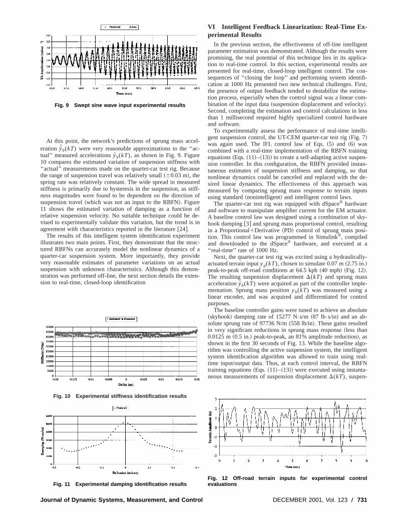
c

ntwerea-

areon-ifi-irst,tima-om-

lessare

lli-

ngn-n-thatde-

wasputs

tor.ky-ng-

a

lly-

e-atrol

lute

go-ental-FN-

At this point, the network’s predictions of sprung mass acceration yb(kT) were very reasonable approximations to the ‘‘atual’’ measured accelerationsyb(kT), as shown in Fig. 9. Figure10 compares the estimated variation of suspension stiffness‘‘actual’’ measurements made on the quarter-car test rig. Becathe range of suspension travel was relatively small~60.03 m!, thespring rate was relatively constant. The wide spread in measustiffness is primarily due to hysteresis in the suspension, as sness magnitudes were found to be dependent on the directiosuspension travel~which was not an input to the RBFN!. Figure11 shows the estimated variation of damping as a functionrelative suspension velocity. No suitable technique could bevised to experimentally validate this variation, but the trend isagreement with characteristics reported in the literature@24#.

The results of this intelligent system identification experimeillustrates two main points. First, they demonstrate that the strtured RBFNs can accurately model the nonlinear dynamics oquarter-car suspension system. More importantly, they provvery reasonable estimates of parameter variations on an asuspension with unknown characteristics. Although this demstration was performed off-line, the next section details the extsion to real-time, closed-loop identification

Fig. 9 Swept sine wave input experimental results

Fig. 10 Experimental stiffness identification results

Fig. 11 Experimental damping identification results


el-c-

withuse

redtiff-n of

ofde-in

ntuc-f aidetual

on-en-

VI Intelligent Feedback Linearization: Real-Time Ex-perimental Results

In the previous section, the effectiveness of off-line intelligeparameter estimation was demonstrated. Although the resultspromising, the real potential of this technique lies in its appliction to real-time control. In this section, experimental resultspresented for real-time, closed-loop intelligent control. The csequences of ‘‘closing the loop’’ and performing system identcation at 1000 Hz presented two new technical challenges. Fthe presence of output feedback tended to destabilize the estion process, especially when the control signal was a linear cbination of the input data~suspension displacement and velocity!.Second, completing the estimation and control calculations inthan 1 millisecond required highly specialized control hardwand software.

To experimentally assess the performance of real-time integent suspension control, the UT-CEM quarter-car test rig~Fig. 7!was again used. The IFL control law of Eqs.~5! and ~6! wascombined with a real-time implementation of the RBFN trainiequations~Eqs.~11!–~13!! to create a self-adapting active suspesion controller. In this configuration, the RBFN provided instataneous estimates of suspension stiffness and damping, sononlinear dynamics could be canceled and replaced with thesired linear dynamics. The effectiveness of this approachmeasured by comparing sprung mass response to terrain inusing standard~nonintelligent! and intelligent control laws.

The quarter-car test rig was equipped with dSpace® hardwareand software to manipulate amplifier current for the EM actuaA baseline control law was designed using a combination of shook damping@3# and sprung mass proportional control, resultiin a Proportional1Derivative ~PD! control of sprung mass position. This control law was programmed in Simulink®, compiledand downloaded to the dSpace® hardware, and executed at‘‘real-time’’ rate of 1000 Hz.

Next, the quarter-car test rig was excited using a hydraulicaactuated terrain inputyg(kT), chosen to simulate 0.07 m~2.75 in.!peak-to-peak off-road conditions at 64.5 kph~40 mph! ~Fig. 12!.The resulting suspension displacementD(kT) and sprung massaccelerationyb(kT) were acquired as part of the controller implmentation. Sprung mass positionyb(kT) was measured usinglinear encoder, and was acquired and differentiated for conpurposes.

The baseline controller gains were tuned to achieve an abso~skyhook! damping rate of 15277 N•s/m ~87 lb•s/in! and an ab-solute sprung rate of 97736 N/m~558 lb/in!. These gains resultedin very significant reductions in sprung mass response~less than0.0125 m~0.5 in.! peak-to-peak, an 81% amplitude reduction!, asshown in the first 30 seconds of Fig. 13. While the baseline alrithm was controlling the active suspension system, the intelligsystem identification algorithm was allowed to train using retime input/output data. Thus, at each control interval, the RBtraining equations~Eqs.~11!–~13!! were executed using instantaneous measurements of suspension displacementD(kT), suspen-

Fig. 12 Off-road terrain inputs for experimental controlevaluations


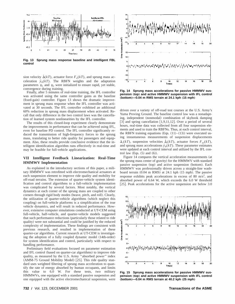
e

eeea

l

rI

u

oio

e

c

t

u

r

w

y’sapt-

lele-rval,

ents

son-

s

h-

old3.0

sion velocityD(kT), actuator forceFa(kT), and sprung mass acceleration yb(kT). The RBFN weights and the adaptatioparametersh1 andh2 were initialized to ensure rapid, yet stablconvergence during training.

Finally, after 5 minutes of real-time training, the IFL controllwas activated using the same controller gains as the bas~fixed-gain! controller. Figure 13 shows the dramatic improvment in sprung mass response when the IFL controller wasvated at 30 seconds. The IFL controller exhibited an additio60% reduction in sprung mass displacement when activated.call that only difference in the two control laws was the cancetion of learned system nonlinearities by the IFL controller.

The results of this closed-loop experiment clearly demonstthe improvements in performance that can be achieved usingeven for baseline PD control. The IFL controller significantly rduced the transmission of high-frequency forces to the sprmass, translating to better ride quality for passengers and eqment. Also, these results provide conclusive evidence that thetelligent identification algorithm runs effectively in real-time anmay be feasible for full-vehicle applications.

VII Intelligent Feedback Linearization: Real-TimeHMMWV Implementation

As explained in the introductory sections of this paper, a mtary HMMWV was retrofitted with electromechanical actuatorseach suspension element to improve ride quality and mobilityoff-road terrains. The extension of quarter-vehicle system idefication and control algorithms to a full-vehicle implementatiwas complicated by several factors. Most notably, the vertdynamics at each corner of the sprung mass are coupled tocorners through rigid body modes~heave, pitch, and roll!. Clearly,the utilization of quarter-vehicle algorithms~which neglect thiscoupling! on full-vehicle platforms is a simplification of the truvehicle dynamics, and will result in reduced performance. Hoever, extensive computer simulations conducted at UT-CEM usfull-vehicle, half-vehicle, and quarter-vehicle models suggesthat such performance reductions~particularly those related to ridequality! were not substantial and could be justified by the reducomplexity of implementation. These findings are consistent wprevious research, and resulted in implementation of thquarter-car algorithms. Current research at UT-CEM is investiging the adoption of a fully coupled dynamic model~14th-order!for system identification and control, particularly with respecthandling performance.

Preliminary field evaluations focused on parameter estimaand IFL control~based on quarter-car algorithms! to improve ridequality, as measured by the U.S. Army ‘‘absorbed power’’ ind~AMM-75 Ground Mobility Model! @25#. This ride quality stan-dard uses weighted filtering of sprung mass acceleration to qtify the rate of energy absorbed by human occupants, and limthis value to 6.0 W. For these tests, two militaHMMWVs, one equipped with a standard passive suspensionone equipped with the active electromechanical suspension,

Fig. 13 Sprung mass response baseline and intelligent FBLcontrol


-n,

rline-cti-

nalRe-la-

ateFL,e-ng

uip-in-

d

ili-atfornti-n

calther

w-ingted

editheseat-

to

ion

ex

an-its

yandere

driven over a variety of off-road test courses at the U.S. ArmYuma Proving Ground. The baseline control law was a nonading, independent~nonmodal! combination of skyhook damping@3# and spring cancellation@1,9,11,12#. Over a period of severahours, real-time data was collected from all four suspensionments and used to train the RBFNs. Thus, at each control intethe RBFN training equations~Eqs.~11!–~13!! were executed us-ing instantaneous measurements of suspension displacemD i(kT), suspension velocitiesDi(kT), actuator forcesFai(kT),and sprung mass accelerationsyb(kT). These parameter estimatewere updated at each control interval and utilized by the IFL ctrol law ~Eqs.~5! and ~6!!.

Figure 14 compares the vertical acceleration measurement~atthe sprung mass center of gravity! for the HMMWV with standardpassive suspension~top! and active suspension~bottom!. EachHMMWV was professionally driven across a straight-line wasboard terrain~0.04 m RMS! at 24.1 kph~15 mph!. The passiveresponse exhibits peak accelerations in excess of 80 m/s2, andabsorbed power of 6.64 W, which exceeds the 6.0 W thresh@25#. Peak accelerations for the active suspension are below

Fig. 15 Sprung mass accelerations for passive HMMWV sus-pension „top … and active HMMWV suspension with IFL control„bottom …—0.04 m RMS terrain at 40.2 kph „25 mph …

Fig. 14 Sprung mass accelerations for passive HMMWV sus-pension „top … and active HMMWV suspension with IFL control„bottom …—0.04 m RMS terrain at 24.1 kph „15 mph …


na

e

nar

t

r

yt

i

e

t

r

m

i3I

a

nU

,

S

r

t

rs

ted..,

nc-

rd

nd

rks

emand

ualmssiststly

andust-tionion.aionri-

less

In-

s

m/s2, and the absorbed power is an incredibly low 0.35 W~a 95%reduction!. Figure 15 is a similar comparison for 40.2 kph~25mph!. The passive response~top! exhibits peak accelerations iexcess of 15.0 m/s2, and absorbed power of 13.85 W, more thtwice the limiting threshold@25#. Peak accelerations for the activsuspension are below 5.0 m/s2, and the absorbed power is a rmarkably low 1.49 W~an 89% reduction!.

VIII Conclusions and RecommendationsThis paper details the development and real-time impleme

tion of intelligent parameter estimation and Intelligent FeedbLinearization~IFL! to improve the ride quality and handling peformance of off-road active suspension systems. The IFL contler combines Radial Basis Function Networks~RBFNs! with anadaptive control strategy to cancel undesired nonlinearities,facilitating the use of linear control laws. Experimental resufrom a quarter-car test rig demonstrate 60% improvements inquality relative to a baseline~non-adapting! controllers. Addi-tional, field trial results from a HMMWV implementation clearldemonstrate the performance of quarter-vehicle parameter estion and control algorithms for improved ride quality. 95% redutions in absorbed power and 65% reductions in peak sprung macceleration have been documented using this IFL approach.

The IFL controller design followed a logical progression froconcept and computer simulation@26#, to real-time experiment, tofull-vehicle implementation. Testing and refinement of the fuvehicle controller, currently installed on a HMMWV, is still underway. Current research at UT-CEM is addressing full-veh~dynamically coupled! control algorithms and bump-stop avoidance algorithms, as the energy transmitted to occupants rheavily on avoiding the shocks associated with travel spacehaustion.

AcknowledgmentsThe authors would like to express their appreciation for

technical assistance of Damon Weeks, Andreas Guenin, andBresie. The authors would also like to acknowledge the suppothe U. S. Army Tank and Automotive Command~TACOM!.

References@1# Beno, J. H., Bresie, D. A., Ingram, S. K., Weeks, D. A., and Weldon, Wm.

1995, ‘‘Electromechanical Suspension System,’’ Final Report to U. S. ArTank and Automotive Command, Warren, MI, June.

@2# Weeks, D. A., Beno, J. H., Guenin, A., and Bresie, D. A., 1999, ‘‘The Desof an Electromagnetic Linear Actuator for an Active suspension,’’ SP-14Steering and Suspension Technology Symposium 1999, SAE, Warren, M

@3# Crosby, M., and Karnopp, D. C., 1973, ‘‘The Active Damper—A New Concefor Shock and Vibration Control,’’ Shock and Vibration Bulletin, Part H.

@4# Hrovat, D., 1997, ‘‘Survey of Advanced Suspension Developments andlated Optimal Control Applications,’’ Automatica33, No. 10, pp. 1781–1817.

@5# Kim, E. S., 1996, ‘‘Nonlinear Indirect Adaptive Control of a Quarter CActive Suspension,’’ Proceedings of the 1996 IEEE International Confereon Control Applications, pp. 61–66.

@6# Williams, D. E., and Haddad, W. M., 1997, ‘‘Active Suspension ControlImprove Vehicle Ride and Handling,’’ Vehicle System Dynamics28, No. 1, pp.1–24.

@7# Moran, A., and Nagai, M., 1994, ‘‘Optimal Active Control of Nonlinear Vehicle Suspensions Using Neural Networks,’’ JSME International Journal,ries C37, No. 4, pp. 707–719.

@8# Nagai, M., Moran, A., Tamura, Y., and Koizumi, S., 1997, ‘‘Identification aControl of Nonlinear Active Pneumatic Suspension for Railway Vehicles,ing Neural Networks,’’ Control Engineering Practice5, No. 8, pp. 1137–1144.

@9# Scheutze, K. T., Beno, J. H., Weldon, W. F., and Sreenivasan, S. V., 1998Comparison of Controller Designs for an Active, Electromagnetic, OffroVehicle Suspension System Traveling at High Speed,’’ presented at theInternational Congress and Exposition, Detroit, MI, Feb. 23–26.

@10# Sunwoo, M., and Cheok, K. C., 1991, ‘‘Investigation of Adaptive ContrApproaches for Vehicle Active Suspension Systems,’’ Proceedings of 1American Control Conference, Vol. 2, pp. 1542–1547.

@11# Weeks, D. A., Beno, J. H., Bresie, D. A., and Guenin, A. M., 1997, ‘‘ContSystem for Single Wheel Station Tracked Vehicle Active Electromagnetic Spension,’’ presented at SAE International Congress and Exposition, DeMI, Feb.

@12# Weeks, D. A., Beno, J. H., Bresie, D. A., and Guenin, A. M., 1997, ‘‘Labotory Testing of Active Electromagnetic Near Constant Force Suspen


ne-

ta-ck-rol-

husltside

ima-c-ass

m

ll--cle-liesex-

heDont of

F.,y

gn8,

.pt

Re-

rnce

to

-Se-

ds-

‘‘AadAE

ol991

olus-roit,

a-ion

~NCFS! Concept on Subscale Four Corner, Full Vehicle Test-Rig,’’ presenSAE International Congress and Exposition, Detroit, MI, February 24–27

@13# Ljung, L., 1991, ‘‘Issues in System Identification,’’ IEEE Control Syst. Magpp. 25–29.

@14# Ljung, L. and Glad, T., 1994,Modeling of Dynamics Systems, Prentice Hall.@15# Astrom, K. J., and Wittenmark, B., 1995,Adaptive Control, 2nd Ed., Addison

Wesley.@16# G. C. Merriam Co., 1991,Webster’s New Collegiate Dictionary, G. C. Mer-

riam Co.@17# Haykin, S., 1994,Neural Networks, A Comprehensive Foundation, Prentice

Hall.@18# Cybenko, G., 1989, ‘‘Approximations by Superpositions of a Sigmoidal Fu

tions,’’ Mathematics of Control Signal Systems 2 pp. 303–314.@19# Hornik, J., Stinchcombe, M., and White, H., 1989, ‘‘Multilayer Feedforwa

Networks are Universal Approximators,’’ Neural Networks2, pp. 359–366.@20# Baker, W. L., and Farrell, J. A., 1992,An Introduction to Connectionist Learn-

ing Control Systems, Handbook of Intelligent Control: Neural, Fuzzy, aAdaptive Approaches, Van Nostrand Reinhold.

@21# Slotine, J. J., and Li, W., 1991,Applied Nonlinear Control, Prentice Hall.@22# Brogan, W. L., 1991,Modern Control Theory, 3rd ed., Prentice Hall.@23# Bruzzone, L., Roli, F., and Serpico, S. B., 1998, ‘‘Structured Neural Netwo

for Signal Classification,’’ Signal Process.64, No. 3, pp. 271–290.@24# Bastow, D., and Howard, G. P., 1993,Car Suspension and Handling, 3rd Ed.,

Society of Automotive Engineers, Inc.@25# Wong, J. Y., 1993,Theory of Ground Vehicles, Wiley, New York, NY.@26# Buckner, G. D., and Schuetze, K. T., 1999, ‘‘Intelligent Estimation of Syst

Parameters for Active Vehicle Suspension Control’’ SP-1438, SteeringSuspension Technology Symposium 1999, SAE, Warren, MI.

Point-to-Point Motion Planning forServosystems With ElasticTransmission Via Optimal DynamicInversion1

Aurelio PiazziDipartimento di Ingegneria dell’Informazione,University of Parma, Parma, Italye-mail: [email protected]

Antonio VisioliDipartimento di Elettronica per l’Automazione,University of Brescia,Via Branze 38, I-25123 Brescia, Italye-mail: [email protected]

A new technique, based on dynamic inversion, for the residvibration reduction in the point-to-point motion of servosystewith elastic transmission is presented. The methodology conof defining a suitable motion law for the load, and subsequendetermining, via dynamic inversion, the corresponding commfunction for the system. The method inherently assures the robness of the control scheme despite inaccuracies in the estimaof the stiffness constant and of the damping of the transmissThe main contribution of the paper lies in the definition ofsimple optimization procedure which allows the system inverspoint that minimizes the residual vibration to be found. Expemental results show that in this way the identification phase iscritical and performances can be significantly improved.@DOI: 10.1115/1.1408944#

Keywords: Oscillatory Systems, Open-Loop Control, Dynamicversion, Optimization

1This work was supported in part by MURST scientific research funds.Contributed by the Dynamic Systems and Control Division of THE AMERICAN

SOCIETY OF MECHANICAL ENGINEERS. Manuscript Received by the DynamicSystems and Control Division October 3, 2001. Associate Editor: C. Rahn.


rdo

r

t

ih

l

tavna

ss

t

i

rs

-

-

fs

d

andtionhisasedr

mo-.

put

ro

e-

nts

sion

be

tio.

-

d as

1 IntroductionHigh performances servosystems might suffer from the p

ence of elasticities in the transmission, which produces a resivibration at the end of a point-to-point motion. This fact intrduces limitations in the reduction of the working cycle time, sinthe oscillation has to vanish before achieving the desired accuof the positioning system. This problem has been addressednumber of researchers in the past and two strategies havefollowed: either implementing a closed-loop control scheme,which the state of the dynamic system has to be known duringmotion ~and therefore apposite sensors have to be adopted! or anopen-loop control scheme which relies on an appropriate moplanning methodology. In the context of the open-loop stratethe input shaping technique has been successfully developedthe last decade~see e.g.@1,2#!. Basically, it consists of convolvinga sequence of impulses, also known as the input shaper, wdesired system command to generate the system command tthen used to drive the system.

In a previous paper@3# we proposed an alternative approachthe input shaping technique. It is based on the concept of dynainversion and it allows minimization of the motion time whitaking into account actuator constraints. The general idea is todefine an arbitrarily smooth closed-form polynomial motion funtion, parameterized by the time intervalt, for the load of thesystem to avoid oscillations during and at the end of the mo@4#. Then, by means of dynamic inversion the actual comminput that causes the desired planned load motion is deriSimulation and experimental results have proven the effectiveof the method, with respect to the input shaping technique,how it is inherently robust to modeling errors.

In this paper, we further develop the system-inversion-bamethodology. Rather than considering a priori the uncertaintiethe model, we perform a simple procedure to search for the omal inversion point to minimize the residual vibration amplitudIn other words, starting from values of the system paramedetermined by means of a simple identification experiment,modify them in the system model adopted for the dynamic invsion, through repetitive experiments, until the residual vibratamplitude is minimized.

2 Dynamic Inversion Based Motion PlanningThe presence of a gearbox in a mechanical positioning se

system generally introduces an elastic element which can beply described by the model shown in Fig. 1 wherey is the coor-dinate representing the motor shaft displacement,x is thecoordinate representing the mass displacement,m is the loadmass,k the stiffness constant, andc the damping of the transmission @5#. The well-known linear relation betweenx andy has thefollowing differential form:

mx1cx1kx5cy1ky (1)

which can be rewritten as:

z12jvnz1vn2z52 y

wherez5x2y, vn5Ak/m rad•s21 is the frequency of the oscillatory mode andj5c/2mvn is the damping ratio.

Fig. 1 Model of an elastic transmission


es-ual-

ceacyby abeeninthe

iongy,over

th aat is

tomicefirstc-

ionnded.essnd

edof

pti-e.ersweer-on

vo-im-

In general~we refer for example to the motion planning oindustrial robot manipulators!, the elasticity of the transmission inot taken into account and the motion is planned ony ~the input ofthe system~1!!, exploiting the full capabilities of the actuator anconsidering the massm rigidly linked to the motor. When, how-ever, excessive vibrations occur, the velocities, accelerationsjerks of the trajectory have to be reduced by increasing the motime and therefore limiting the performances of the system. Tdrawback can be overcome by adopting a system-inversion-bmethodology which will be briefly described in the following. Fodetails see@3#.

Define a point-to-point motion law from position 0 toq for theload in the time interval@0,t# using the ‘‘transition’’ polynomialsintroduced in@4#:

x~ t;t!5q~2h11!!

h! t2h11 (i 50

h~21!h2 i

i ! ~h2 i !! ~2h2 i 11!t i t2h2 i 11. (2)

Outside the interval@0,t#, x(t;t) is simply defined asx(t;t)50 ift<0 andx(t;t)5q if t>t. In ~2! the integerh can be arbitrarilychosen in order to assurex(t;t)PC(h) over R, i.e., x(t;t) hascontinuous derivatives up to thehth order. Note thatx(t;t) ismonotonically increasing and as a consequence, the plannedtion of the massm is, by construction, free of oscillatory modes

Consider the transfer function of the system~1!:

G~s!5X~s!

Y~s!5

cs1k

ms21cs1k(3)

Applying the Laplace transform operatorL both to y(t;t) andx(t;t), the closed-form expression of the parameterized infunction for t>0 ~obviouslyy(t;t)50 if t,0! which causes thedesired output function can be calculated as:

y~ t;t!5L21@G21~s!X~s;t!#5m

cx~ t;t!1S 12

mk

c2 D x~ t;t!

1mk2

c3 e2~k/c!tE0

t

e~k/c!vx~v;t!dv. (4)

Note thaty(t;t) is all over bounded because the excited zemodee2(k/c)t is stable. In order to obtainy(t;t) belonging toC( l )

it is necessary that, by virtue of~4!, x(t;t) belong toC( l 11), i.e.,h5 l 11. In particular, to at least ensure the continuity of the vlocity input function, the constrainth>2 must be satisfied.

At this point the optimization procedure described in@3# for theminimization of the motion time subject to actuator constraican be readily applied.

3 Dynamic Inversion Point OptimizationIn the previous section it has been exposed a dynamic inver

based synthesis of the motion input that depends, besidest, on theparametersm, c, andk. In particular, the linkage parametersc andk, which are not exactly known in many practical cases, canexplicitly indicated as formal parameter arguments iny(t;c,k,t).Thus, the problem of the optimal selection ofc>dc andk>dk iny(t;c,k,t) arises, wheredk and dc are given arbitrarily smallpositive values of the natural frequency and of the damping raWe propose to choosec andk in order to minimize the amplitudeof the actual residual vibration~the transient motion of the loadfor t>t!. Application of inputy(t;c,k,t) to the actual servo determines an output motion denoted asx(t;c,k,t). Hence, the re-sidual vibration amplitude can be defined as:

J5J~c,k!ªmaxt>t

ux~ t;c,k,t!2qu. (5)

The addressed motion planning problem is therefore posethe following minimization problem:


aro

a

n

e

t

on

gt

l,n

o

a

of

ndis

rorur-

etheThe

minc>dc ,k>dk

J~c,k!. (6)

Searching for a global solution of the optimization problemextremely difficult because it has to be solved by means of sably arranged experimental trials. Therefore, we propose a prcable local optimization procedure based on a simplified coonate descent method@@6#, p. 227# which is in any case capable tsignificantly improve the control system performances. Hence,minimizersc* andk* of problem~6! can be found by means othe following optimal inversion point~OIP! procedure.

OIP Procedure

1 Perform an identification experiment and estimatek0 andc0~initial values!.

2 Setk* 5k0 , c* 5c0 , flag50.3 Perform an experiment and setIªJ(c* ,k* ) and I 15I .4 Setk* 5(11«)k* .5 Perform an experiment and setIªJ(c* ,k* ).6 If I ,I 1 then set flag51 and go to 3.7 If flag51 go to 11.8 Setk* 5(12«)k* . If k* ,dk then setk* 5dk .9 Perform an experiment and setIªJ(c* ,k* ).10 If I ,I 1 then go to 8.11 Set flag50.12 Setc* 5(11«)c* .13 Perform an experiment and setIªJ(c* ,k* ).14 If I ,I 1 then set flag51 and go to 12.15 If flag51 go to 19.16 Setc* 5(12«)c* . If c* ,dc then setc* 5dc .17 Perform an experiment and setIªJ(c* ,k* ).18 If I ,I 1 then go to 16.19 End.

The typical identification experiment that can be performedstep 1 might consist of applying a torque impulse to the motoranalyzing the oscillatory response of the load. From the evaluaof the frequency and of the decay ratio of the response, the sness constant and the damping ratio can be straightforwadetermined.

Parameter« determines the velocity of the descent to the mimum and the precision in determiningk* and c* . It is easy toadapt it in order to have a fast descent to the minimum atbeginning and then increasing the accuracy once we are closit ~for example, on the practical grounds,« can be initially fixed to0.05!.

Remark 1. It is very important to stress that the resulting opmal parameters do not necessarily coincide with the real valuethe parameters of the physical system. In other words, minimizthe residual vibration does not mean in general that we havecurately identified the stiffness constant and the damping ratithe system, since nonlinear effects, which are inevitably presethe system, are not included in the simple model~1!.

4 Experimental Setup and ResultsThe experimental setup consists of a testbed, depicted in Fi

in which two carts, linked by a spring, slide on a stainless srectilinear guide~see Fig. 3 for a detail of the two carts!. The firstcart is connected to a belt which is moved through some pulby means of a brushless motor configured in torque mode, i.e.signal given to the drive by the controller is a torque commaThe overall reduction rate of the transmission system is knoand therefore, we assume that the input reference functiony(t) isthe position of the first cart, rather than the position of the moshaft.

Then, the positiony(t) of the first cart is measured by meansan incremental encoder, mounted on the motor shaft, whose rlution is 4•1000 impulses per motor revolution. The second c


isuit-cti-di-

thef

atnd

tiontiff-rdly

i-

thed to

i-s ofingac-of

t in

. 2,eel

eysthed.

wn

tor

feso-rt,

whose mass is 0.8 kg, is not actuated and its positionx(t) ismeasured with an incremental linear scale with a resolution40 mm.

The control system is implemented in a PC with I/O boards athe control frequency is 1 kHz. The position of the first cartcontrolled by a standard Proportional-Integral-Derivative~PID!controller which has been accurately tuned by a trial and erprocedure, in order to guarantee a very low positioning error ding the motion.

A simple identification experiment, in which a torque impulswas applied to the first cart and the oscillatory response ofsecond cart has been analyzed, has been initially performed.

Fig. 2 Sketch of the experimental setup

Fig. 3 The two carts linked with the spring adopted for theexperiments

Fig. 4 The planned motion of the load


t

f

icut

alhatre.

ed

t inre-

s-that

litytheat a

anlowspitepti-the

m-thein-ntal

re-

ionon-

o-.,

of

ngVi-

resulting values ofk0 and c0 were 1858.15 kg•s22 and 8.03kg•s21, respectively, which corresponds to a nominal natural fquency of 48.19 rad•s21 and a nominal damping ratio of 0.10Then, a load motion ofq50.2 m to be accomplished int50.3 swas planned~see Fig. 4!. The value of the motion time have beeselected in order to exploit the full dynamics of the actuator, wiout saturating. A polynomial output function of fifth order (h52) has been adopted, in order to guarantee the continuity oinput function until the first order, i.e., discontinuities in the aceleration reference signal are allowed. Thus, we have:

Fig. 5 The command input function for the nominal and opti-mal dynamic inversion

Fig. 6 The actual load motion for the nominal and optimal dy-namic inversion


re-.

nh-

thec-

x~ t !50.2S 6

0.35 t5215

0.34 t4110

0.33 t3D .

Then, the OIP procedure has been applied, having fixeddc

5dk51024. At the end, it results ink* 53000 andc* 50.001,that is, a natural frequency of 61.24 rad•s21 and a damping ratioof 1.02•1025. The resulting input function, obtained via dynaminversion, is plotted in Fig. 5, where it is compared with the inpfunction obtained by inverting the nominal system withk0 andc0 . The actual load motions for both the nominal and optimdynamic inversion are plotted in Fig. 6, where it appears tsignificant improvement is achieved by using the OIP proceduNote that the objective functionJ is reduced from 2.7•1023 m to0.6•1023 m. Moreover, the steady-state value of 0.2 m is attainat t50.4 s for the optimal case and att50.54 s for the nominalone.

5 ConclusionsIn this paper we have presented an important developmen

the system-inversion-based technique for the reduction of thesidual vibration in point-to-point motion of mechanical servosytems endowed with elastic transmissions. It has been shownthe use of the dynamic inversion methodology provides flexibiin the motion planning design, as it allows to easily cope withactuator limits. Moreover, the identification phase can be keptvery simple level, as the use of the polynomial functions ensureinherent robustness to the system and the OIP procedure alachieving high performances straightforwardly. Indeed, desthe simple modeling of the system and the simple adopted omization procedure, significant results have been obtained andimprovement with respect to the previously defined systeinversion-based methodology is evident. The readiness ofoverall methodology makes it very suitable to be adopted industrial environments, as demonstrated by the experimeresults.

References@1# Singer, N. C., and Seering, W. P., 1990, ‘‘Preshaping command inputs to

duce system vibration,’’ ASME J. Dyn. Syst., Meas., Control,112, Mar., pp.76–82.

@2# Singhose, W. E., Porter, L. J., Tuttle, T. D., and Singer, N. C., 1997, ‘‘Vibratreduction using multi-hump input shapers,’’ ASME J. Dyn. Syst., Meas., Ctrol, 119, June, pp. 320–326.

@3# Piazzi, A., and Visioli, A., 2000, ‘‘Minimum-time system-inversion-based mtion planning for residual vibration reduction,’’ IEEE/ASME Trans. on Mech5, No. 1, pp. 12–22.

@4# Piazzi, A., and Visioli, A., 2001, ‘‘Optimal noncausal set-point regulationscalar systems,’’ Automatica,37, No. 1, pp. 121–127.

@5# Adamini, R., Faglia, R., and Incerti, G., 1995, ‘‘Parametric motion plannitechniques for servosystems endowed with elastic transmission,’’ Machinebration,4, pp. 14–21.

@6# Luenberger, D. G., 1989,Linear and Nonlinear Programming, Addison Wes-ley, Reading.


Technical Briefs - unipr.it · PDF fileTechnical Briefs An Inﬁnite ... Mechanical...

Documents

Transcript of Technical Briefs - unipr.it · PDF fileTechnical Briefs An Inﬁnite ... Mechanical...