,f~

ARL-TR-W15"14 ,,p ,

AN EXPERIMENTAL INVESTIGATION OF ACOUIA;qi T3OWIN SATURATED SAND WITH VARIABLE FL UI•.|FI *du1=

R. Daniel Costley, Jr.

UX)It)

APPLIED RESEARCH LABORATORIESTHE ••NIVERSITY OF TEXAS AT AUTIN

MEST OFFICE SOX S0M., AUSTIN. TEXAS 727134MMI

May 1985

Technical Report

Approved for public release;distribution unlimited.

Prepared for:

OFFICE OF NAVAL RESEARCHDEPARTMENT OF THE NAVY

ARLINGTON, VA 22217

0.

* DTICA"k.ELECTS

1qNOCT 9 1980

85 10 9 083

~~~~v ... r L ,t . . . . ,'• , • - , . •_ . • _ "

UNCLASSIFIEDSECURITY CLASSIFICATION OF THIS PAGE (When Datarnfored)

READ INSTRUCTIONSREPORT DOCUMENTATION PAGE BEFORE COMPLETING FORM

1. REPORT NUMBER 12.jGOVT ACCESSION NO. 3. RECIPIENT'S CATALOG NUMBER

4. TITLE (and Subtitle) S. TYPE OW REPORT & PERIOD COVERED

AN EXPERIMENTAL INVESTIGATION OF ACOUSTICPROPAGATION IN SATURATED SANDS WITH VARIABLE 6. PERFORMING ORG. REPORT NUMBER

FLUID PROPERTIES ARL-TR-85-147. AUTHOR(#) 8. CONTRACT OR GRANT NUMBER(#)

R. Daniel Costley, Jr. NO0O14-80-C-0490

9. PERFORMING ORGANIZATION NAME AND ADDRESS 10. PROGRAM ELEMENT. PROJECT, TASK

Applied Research Laboratories AE& WOR UNIT NUMBERS

The University of Texas at Austin technical reportAustin, Texas 78713-802911. CONTROLLING OFFICE NAME AND ADDRESS 12. REPORT DATE

Office of Naval Research May 1985Department of the Navy 13. NUMBER OF PAGES

Arlington, Virginia 22217 1O00_14. MONITORING AGENCY NAME & ADDRESS(Il dillferent from Controlling Office) IS. SECURITY CLASS. (of this reprt)

UNCLASS I FI ED

ISa. DECL ASS: FICATION/ DOWNGRADINGSCHEDULtE

16. DISTRIBUTION STATEMENT (of this Report)

17. DISTRIBUTION STATEMENT (of th. abstract entered in Block 20, if different from Report) ' I

Approved for public release; distribution unlimited. ELECTE

18. S U P P _LE'ME"NT A RY T,0"E S • OT• ~

7A

19. KEY WORDS (ContInue on roeveres side If necessary end identify by block number)

;ompressional velocity- experiment,compressional attenuation, sand"riot theory;viscosity dependence.

20. ABSIRACT (Continue on reverse side If necessary and Identify by block number)

-The Biot-Stoll theory describes the propagation of acoustic waves in a saturatedunconsolidated porous medium. The expressions for the attenuation and phasevelocity derived from this theory depend explicitly on the viscosity, density,and bulk modulus of the pore fluid. An experiment has been designed to determin(the dependence of attenuation and phase velocity on these properties of the porefluid. The phase velocity and attenuation of compressional waves were measuredusing a mixture of water and glycerine as the interstitial fluid. The theore-tical background is reviewed and the experimental procedure is discussed in

DD IJAN73 1473 EDITION OF I NOV6S IS OBSOLETE UNCLASSIFIEDSECURITY CLASSIFICATION OF THIS PAGE IWhen Data En ted)

UNCLASSIFIEDSECURITY CLASSIFICATION OF THIS PAGE(Whmi Date Entered)

20.,.(cont,'d)

• detail. The results, alorg with comparisons with the Biot-Stoll theory,are then presented. The choices of the theoretical parameters are discussedand their relation to the fit of the theory to the data. The Biot-Stolltheory is shown to adequately describe the effects of the fluid propertieson acoustic wave propagation in saturated sediments, at least for .. 'compressional waves of the first type. /

S., : .%. p

UNCLASSIFIEDSECURITY CLASSIFICATION OF THIS PAGE("Whn Dal& Entered)

.. ,; -. ..-. .. " .. , .. . .. , '.... .... -,, .- ,... ... ... '. ' .% ,•', .. .. ..-.. •:.' ,'-'.' ',• .' ,.*- -, , -. " "•

TABLE OF CONTENTS

Page

LIST OF TABLES vLIST OF FIGURES vii

I. INTRODUCTION I

II. THEORETICAL BACKGROUND 4

Ill. LABORATORY EQUIPMENT 11

A. General Procedure II

B. Instrumentation 13

C. Transducers 15

1. Construction 15

2. Geometrical Spreading 17

3. Directivity 20

D. Sediment Preparation 24

IV. EXPERIMENTAL PROCEDURE 29

A. Phase Velocity 9For 2

B. Attenuation NT13s CRA&IM 35DTIC TAB1. Measurement Technique ut 35.c3J .t. ...

2. Comparison of Results ... .. 44

3. Transient ConsiderationE Cy

4. Effects of Dispersion 54

Dr t

V. EXPERIMENTAL RESULT 56

A. Physical Properties of the Sediment 56

B. Comparison of Results 62

VI. DISCUSSION AND CONCLUSIONS 69

APPENDIX A - COMPUTER PROGRAM 72

APPENDIX B - EXPERIMENTAL DATA 79

REFERENCES 95

iv

t.__

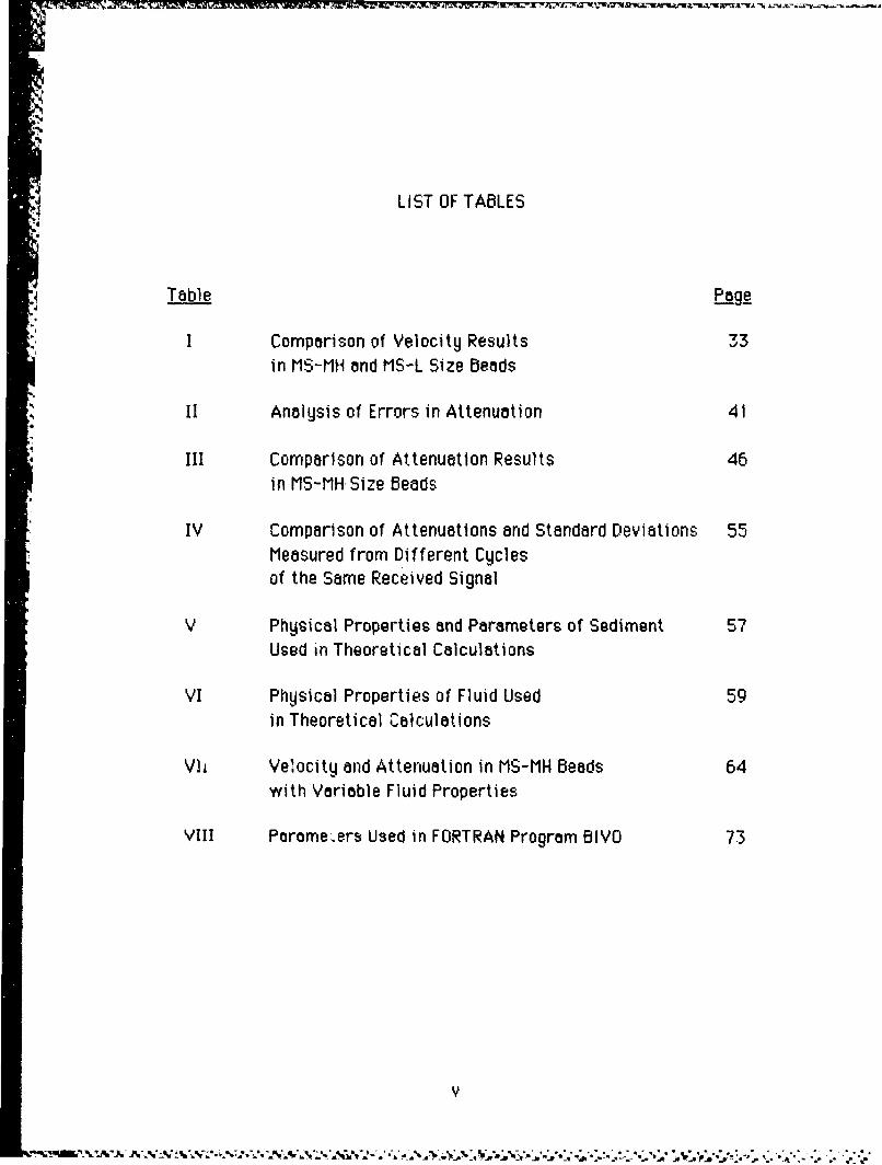
L IST OF TABLES

Table Pg

.,Comparison of Velocity Results 33in MS-MtH and MS-L Size Beads

II Analysis of Errors in Attenuation 41

III Comparison of Attenuation Results 46in MS-MHH Size Beads

IV Comparison of Attenuations and Standard Deviations 55Measured from Different Cyclesof the Same Received Signal

V Physical Properties and Parameters of Sediment 57Used in Theoretical Calculations

VI Physical Properties of Fluid Used 59in Theoretical Calculations

V1i Velocity and Attenuation in MS-MH Beads 64with Variable Fluid Properties

VIII Porameers Used in FORTRAN Program BIVO 73

v

I. INTRODUCTION

There has been continued interest in acoustic propagation in

fluid saturated, poruus media for the post three decades. Initially, much

of the interest was due to problems encountered in the oil industry.

Acoustic techniques were devised, and are still being developed and used,

to determine the properties of the porous rocks, and their interstitial

fluids, found at different depths in oil wells. Maurice Biot, while

working for Shell Development Company, published two papers in 1956

and a third in 1962 describing wave propagation in fluid saturated,

porous, elastic solids. This theory was used to model wave propagation

in fluid saturated, porous rocks where the individual grains are cemented

together.

Since then, there has been interest in accurately describing

wave propagation in unconsolidated, fluid saturated, porous media, such

as water saturated sands. This topic has widespread application in

marine seismic surveys and in sonar and underwater acoustics, since

portions of the ocean bottom consist of water saturated sand. It is also

of interest to soil mechanicists, who use seismic methods to determine

the structural properties of sands and soils, both onshore and offshore.

To predict the acoustic properties of these unconsolidated

sediments, R. D. Stoll extended Biot's original theory to take into account

the losses at the grain-to-grain contacts by proposing that some of the

constitutive coefficients in Biot's equations be made complex (Stoll,

7V I...

1974). Thus, he modeled the solid matrix as a viscoelastic, porous solid,

rather than as the porous, elastic solid considered in Biot's original

work.

Due to the difficulties encountered when making measurements

in saturated sediments, only a limited amount of data exists in

publication. Some published data on unconsolidated, fluid saturated,

porous media have been produced bg R. D. Stoll (Stoll, 1974), David Bell

(Bell, 1979), D. J. Shirley (Shirley, 1978; Bedford, 1982), and Jens Hovem

and G. D. Ingram (Hovem, 1979). More measurements need to be taken,

however, both to validate the theory and to determine the physical

properties of the sediments.

The present experiment, first proposed by D. J. Shirley,

investigates the dependence of the attenuation and phase velocity of

compressional waves in a saturated sand on the properties of the

interstitial fluid. A mixture of glycerine and water was used as the

saturating fluid to permit the controlled variation of the viscosity,

density, and bulk modulus of the pore fluid. Since these parameters

appear explicitly in the Biot-Stoll equations, this investigation provides

a critical test of the theory. Furthermore, the measurements also

provide an estimate of some of the constitutive coefficients in the

equations.

Similar measurements have been made by Shirley, and later by

Elliot (Bedford, 1982). Due to large experimental uncertainties in their

results, no definite conclusions could be made. After investigating their

procedure, a few simple modifications have been made. New

2

..

measurements have been taken and shown to be repeatable within

experimental uncertainties.

The most significant development over the earlier work resulted

from the redesign of the compressional wave transducers. With this

improvement, the existence of spherical spreading was established at

the separations at which these measurements were taken and the error

caused by the directivity of the transducers was reduced.

Both Shirley and Elliot made shear wave measurements in their

investigations. Although it would have been desirable to have measured

the attenuation and phase velocity of shear waves, it was decided that

we could not substantially improve their earlier results without

considerable additional investment in time and effort. Therefore, only

compressional wave propagation was considered in this investigation.

This report is organized as follows. A short review of the

theory for the compressional wave case is presented in Chapter II. In

Chapters III and IV, the experimental procedure is discussed and some of

the assumptions are justified. We compare our results to those of other

investigators in Chapters IV and V, and in Chapter V our results are

compared with the theory.

3

II. THEORETICAL BACKGROUND

In three articles published in The Journal of the AcousticalSociety of America, two in 1956 and the third in 1962, M. A. Biot

presented a theory describing the propagation of acoustic waves in a

fluid saturated, porous, elastic solid (Biot, 1956a, 1956b, 1962). In this

theory, dissipation due to scatter is neglected, requiring that the

wavelength be large in relation to the pore size.

Biot predicted three types of body waves in an unbounded,

porous medium: two types of compressional waves and one shear wave.

All three of these have been observed experimentally. The first type of

compressional wave and the shear wave are analogous to the waves

predicted by ordinary elasticity. The second type of compressional wave

is more dispersive and highly attenuated (Stoll, 1974, 1977).

In Biot's theory, the solid matrix is an elastic frame in which

there is no relative motion between the grains. Later, Stoll and Bryan

extended this theory to include unconsolidated porous media, such as

sands and sediments. Thus, they incorporated into the theory the

inelastic nature of the frame, which is caused by the relative motion of

the grains.

In the Biot-Stoll theory, losses are attributed to three

mechanisms. There are fristional losses at the groin-to-grain contacts.

Secondly, the movement of grain particles relative to one another

produces fluid motion in their immediate vicinity that does not

4

4

contribute to the propagation of the wave. This local fluid motion is at

the expense of the propagating wave, and thus it constitutes a loss

mechanism.

The third type of loss mechanism, and the one which is thought

to dominate in this study, is due to viscous losses in the fluid This type

of absorption becomes important if there is significant motion between

the fluid and the skeletal frame. This effect dominates at higher

frequencies or in sediments where the permembility is high. For

instance, this effect will become more important at lower frequencies

for coarse sands than it would for finer sediments and clays, which have

a lower permeability.

The main purpose of this report is to compare the experimental

measurements of attenuation and phase velocity with the predictions of

the theory. What follows is an outline of the derivation of an expression

for the wave number from Biot's equations. It will serve only to acquaint

those already familiar with the theory with our method of calculating

the phase velocity and attenuation, should there arise any discrepancies

between our results and those of others. For a more complete

discussion, the reader should consult the references by Biot, Stoll,

Bedford, and Hovem and Ingram.

In order to present Biot's equations, some of the notation used

needs to be introduced. If we let u and U represent the displacement

fields of the solid skeletal frame and the fluid, respectively, and if . is

the porosity, then we can write

5

S.

e = divu= V -u

and : div (u- U) V u- U)

Thus, e represents the dilation of an element attached to the frame, and

• represents "the volume of fluid that has flowed in or out of an element

of volume attached to the frame" (Stoll, 1974). The mass density of the

fluid-solid mixture is

p = 1 -$ )P5 + $Pt

and Pc = Pf/• f Cif2

where ps and pf represent the density of the solid and fluid,

respectively.

The drag and virtual mass coefficients are b and c, respectively.

Hovem and Ingram (Hovem, 1979) evaluated b and c as funtions of

frequency and showed that

b / -2 R e a l F W / 8 0

Clf 2 'q Imaginary F(xc)/(WBe)

where K 2 a p 2 ( Wjfl )1

T -( represents the viscosity, u is the angular frequency, and eo is the

permeability. The term ap, which represents a pore size parameter, is

given by

a p dm/U3 1 -$)

and dm is the diameter of the spherical grains of the sediment The

6

.5

IT

function F(c) can be evaluated in terms of the Kelvin function T(c)

- T(K)/4

•'."2 T(x)/,

The Kelvin function, is given by

ber'(1) + i bei'(x)T(x)

ber(W) + i bei(x)

The functions ber(c) and bei(x) are the real and imaginary parts of the

zero order Bessel function of the first kind

ber(W) + i bei(x) = JO ( x" ei 3 TI14 )

The functions ber'(W) and bei'(W) are the derivatives of ber(W) and bel(K),

respectively.

Biot's equations contain several constitutive coefficients which

can be evaluated in terms of the moduli of the solid matrix and the solid

and fluid constituents. The bulk modulus of the drained, solid frame, Kb,

and the shear modulus of the drained, solid frame, ji, are made complex

in order to account for the inelastic response of the frame. The bulk

modulus of the solid and fluid constituents are denoted Ks and Kf

respectively. In terms of these parameters, the constitutive

coefficients in Blot's equations can be written (Stoll, 1974)(K s - Kb )2

H =+Kb + 4P3 ,

D - Kb

7

----- - -.. -...- . . . . . . . -

Ks ( K• -(Kb)

C-D - Kb

Ks 2

and MK=D- Kb

where D=KsI+$(-I+ K Kt)1

With this short introduction to the notation, Mlot's equations for

compressional waves can be written

a2

-(pe- pft) V2 (He-C )at 2

82 b at-(pfe - Pc V2 (Ce - M4 )+ -

at2 $2 atTo find expressions for the phase velocity and attenuation,

harmonic plane wave solutions are assumed for the dilation, e, and the

increment of fluid content, t, as follows&

e = KI exp i(wt - kx)

= K2 exp i(wt - kx) (11-1)

where Ki and K2 are arbitrary constants. Upon substitution into Blot's

equations, the wave number, k, can be solved for in terms of the other

parameters. In general the wave number is complex. The phase velocity,

co and the attenuation, o, can be found from the real and Imaginary parts

8

2 of the wave number by the following relations:

Re(k) = w/Co and Im(k) -o

Substituting equations (It-I) into 3iot's equations leads to two

algebraic equations in e and ý which can be written

2(- +2 p k2H)e + ( 2p f-k 2 C)2C 0

(-. 2pf+k 2 C)e + (-W2pC-k2M -ibW/° 2 ) = 0 .

In order that nontrivial solutions to this system of equations exist, it is

required that the determinant of the coefficients vanish. Solving this

determinant leads to a fourth order algebraic equation in k

Ai k4 + A2 k2 + A3 = 0

where A1=C2 -MH .

i A2 = 2 (pM + pcH - 2pfC ) - i wHb/• 2

and A3 (pw3 )b/ z2 + W4 ( pr2 - PPc •

The roots to this equation are given by the quadratic formula

k2 = (-A 2 ti (A22 - 4A1A3) I / 2A, (11-3)

This represents four roots, two positive and two negative.

The two positive roots correspond, to two different

compressional waves. The value of k calculated from the negative value

of the discriminant, - /(A 22 - 4A1A3), corresponds to the compressional

wave of the second type, or the compressional slow wave. Since the

present experiments are designed to measure the velocity and

9

:•,,..,,,.,".,•.,.•.••,, ,",.,,,'•,, .',•"...•'. ',•,•.]•,,,,,,%.•',,.•'•'•..--.;.•..•. .,.....,..,.-.-.......,.,.............-..,.....-.-...'.-....-....-.. ..

'4-

.4W

attenuation of thE. compressional wave of the first type, the wove

number was calculated with the positive discriminant.

The FORTRAN program shown in Appendix A was used in order to

solve the quadratic formula (11-3) with coefficients (11-2) as a function

of viscosity. The program displays the results in graphical form. In

order to solve for the wave number, and thus the phase velocity and

attenuation, the physical parameters of the saturated sediment need to

be determined. This process is discussed more fully in Chapter V. In the

next two chapters the, procedure used to measure these quantities is

discussed in detail.

10

III. LABORATORY EQUIPMENT

A. Gener Pe ur

The objective of this experiment is to determine the phase

velocity and attenuation of harmonic, compressional waves in a fluid

saturated sediment as a function of the properties of the pore fluid.

These results will be compared with those predicted by the Biot-Stoll

theory. Since the fluid viscosity, bulk modulus, and density appear in the

expression for the wave number, these measurements are expected to be

a critical test of the theory.

Similar measurements of the acoustic properties of sediments

have been performed by Bell (Bell, 1979), Shirley, and Elliot

(Bedford,1982). The main focus of the work described in this chapter and

the next has been to improve the techniques developed by these

investigators for measuring the attenuation and phase velocity of

compressional waves and to Iccate the causes of experimental error. The

most significant improvement over the earlier work has resulted from

the redesign of the compressional wave transducers. With this

improvement, spherical spreading was established at the separations at

which these measurements were taken and the error caused by the

directivity of the transducers was reduced.

The two transducers are essentially identical. One serves as a

transmitter and the other as a receiver. The transmitter converts an

electrical signal, which is generated in an oscillator, into an acoustic

signal, which propagates through the sediment. The receiver detects this

11

acoustic signal and reconverts it into an electrical signal which is

displayed on an oscilloscope.

The central idea in our measurement procedure is to compare

the time delay and amplitude of the output voltage signal at one

transducer separation with the some measurements at other separations.

From the time delay measurements at different separations, the phase

velocity is determined. Similarly, by comparing the different amplitude

measurements, the attenuation can be calculated. It is assumed that the

separation. Thus we assume that the decay in amplitude is due only to

the increase in transducer separation.

Initially, the transducers are placed 20.0 cm apart. The time

delay from the beginning of the triggered pulse to the fourth positivepeak of the received signal is then recorded along with the peak-to-peakamplitude of the fourth cycle of the received signal. The fourth cycle is

I'INused so that the measurements are made as close to the steady state

part of the signal as possible. The signal is then monitored for at least

four hours to ensure that there are no variations in the signal amplitude

due to changes in the coupling between the sediment and the transducers

or due to any settling of the sediment. Four to six readings are taken

over this period, and the slight variations about the stabilized value are

averaged. The receiver is then moved 2.0 cm closer to the transmitter

and the amplitude and time delay measurements are repeated. The entire

procedure is repeated at 2.0 cm intervals until the separation between

the transducers has been reduced to 6.0 cm. Using this set of

12

s. . `:/;• • • `.`;.• •• -? i .. `.;`..> . .. .,...-.,-- • -;- '.'.'---..,,.x -- ,• •

'In

measurements, the phase velocity and attenuation are determined by

finding the least squares fit to the data.

The fluid properties are then altered by adding glycerine to the

mixture. The entire set of measurements is repeated and the phase

velocity and attenuation are determined for a new value of viscosity.

This procedure is repeated several times, each time with a new value of

viscosity. In this way, plots of phase velocity and attenuation versus

viscosity can be made and then compared with predictions of the theory.

B. Instrumentation

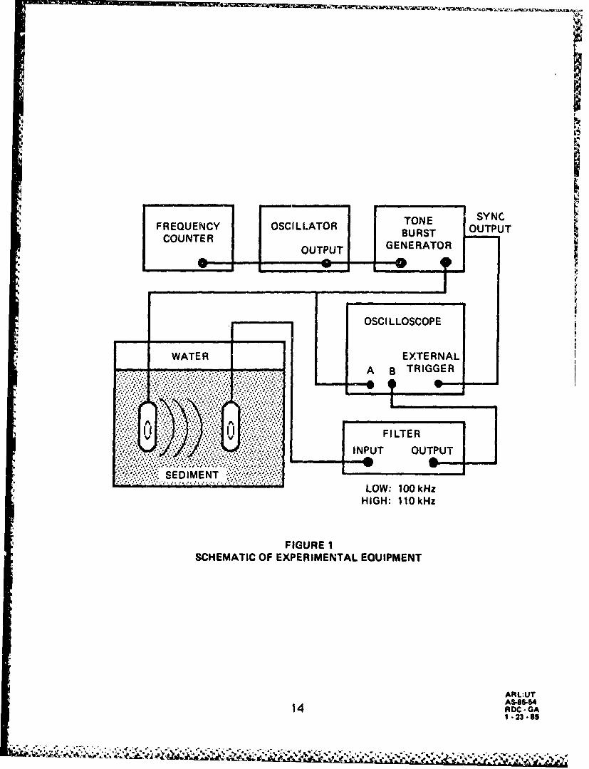
A schematic of the laboratory equipment is shown in Fig. 1. A

continuous tone of 105.0 kHz and 10.0 v peak-to-peak amplitude is

generated in the oscillator. The output is sent to a frequency counter and

a tone burst generator. The tone burst generator pcsses a four cycle

pulse of 105.0 kHz to a transmitting transducer and an oscilloscope. The

signal is then cut off for several milliseconds so that the reflections of

the signal off of the sides of the container and the sediment-water

interface will die down before a new four cycle pulse is sent to the

transmitter. If the reflections are not suppressed, they will interfere

with the signal that follows the direct path between the transducers and

produce an error in the signal amplitude and time delay measurements.

The pulse is also displjyed on an oscilloscope. The tone burst

generator has a synchronized output, which is connected to the external

13

- pTONE 1SYNCFREQUENCY OSCILLATOR BURST OUTPUT

CUTROUTPUT GENERATOR

OSCILLOSCOPE

*WATER EXTERNAL

~•~i~. EDIENTLOW: 100 kHz

HIGH: 110kHz

FIGURE 1SCHEMATIC OF EXPERIMENTAL EQUIPMENT

ARL:UTArb-85-54

14 ADC -GA

trigger input of the oscilloscope. This causes the oscilloscope trace to

trigger at the beginning of the four cycle pulse.

The acoustic pulse generated in the sediment is then detected by

the receiving transducer. The transducer translates the acoustic signal

into a voltage which is sent through a bandpass filter and then displayed

on the oscilloscope. The low and high cutoff frequencies of the bandpass

filter are 100 kHz and 110 kHz, respectively. The filter is used to

remove the extraneous frequencies, introduced because the transmitted

pulse is the product of a pure tone and the difference of two step

functions, from the received signal.

C. Transducers

1. Construction. The two transducers are nearly identical and

can be used as either transmitters or receivers. The transducers were

built from a piezoelectric element mounted in a stainless steel plate.

A rod was welded onto the plate so that the plate and transducer

element could be inserted into the sediment-water mixture. A sketch

of a transducer mount is shown in Fig. 2.

The two elements are made of the material Channelite 5500 and

manufactured by Channel industries, Inc. Their thickness and diameter

are 3/16 in. and 3/4 in., respectively. They each have two resonances.

In the thickness mode, * I and #2 resonate at 446.4 kHz and 445.2 kHz,

respectively. In the radial mode, *1 and *2 resonate at 105.5 kHz and

105.1 kHz, respectively. In this experiment, the transducers are used

in the radial mode, at 105.0 kHz.

15

METALROD

STAINLESSSTEELPLATE

4 in. •0.75 in.

PIEZOELECTRIC_.• -3 i ELEMENT "i

FIGURE 2DIMENSIONS OF TRANSDUCERS

16 ARL:UTAS-85-55RDC - GA1 • 23 - 85

To build the transducers, a 7/8 in. hole was drilled through the

steel plate. The element was placed in the hole with corprene placed

between it and the steel plate, around the circumference of the element,

and behind it on the backside of the transducer. A wire was soldered on

each face of the element, and the two wires were placed in a shielded,

waterproofed sheath.

The corprene is of much lower acoustical impedance than either

the piezoelectric element or the sediment-water mixture. It was thus

used on the backside of the element to act as a pressure release material

so that most of the radiation would be from the front side of the

transducer. This directs most of the energy toward the receiver,

producing a higher signal to noise ratio.

The area of the plate was made sufficiently large and thick, and

the shape of the element was chosen to be circular, so that radiation

from the transducer could be treated as radiation from a piston in a rigid

baffle. In this way the geometrical spreading and the directivity of the

transducer could be calculated and verified by measurement.

2. Geometrical Spreading. Since the geometrical spreading in

the nearfield is very complicated and varies with distance from the

source, the transducers were designed for use in the farfield. The

Rayleigh distance is roughly the distance away from the source at which

the farfield begins. At separations larger than the Rayleigh distance., the

amplitude of the signal decays as 1/r, due to the geometrical spreading

of the signal.

17

The Rayleigh distance for a circular piston in an infinite, rigid

baffle is given by (Blackstock)

R = 112 ka2

where a is the radius of the piston, k=(o/c 0 is the wave number, ,9nd o.) is

the angular frequency. Note that R is inversely proportional to the phase

velocity co. For these transducers, and a frequency of 105.0 1k1z, this

formula gives a Rayleigh distance of 2.0 cm in water. Thus. spherical

spreading is expected at separations of about 4.0 cm or greater.

For a lossless medium in which there is I/r spreading, the

signal amplitude satisfies the following relation:

E KX

Er r

where E is the signal amplitude, Er is a reference amplitude, X. is the

wavelength, and K Is a calibration constant. Taking the logarithm of both

sides gives

E rlog- -log - logK.

El-

Thus, if the si•nal amplitude is measured as a funk (ion of

separation for separations greater than the Rayleigh distance, tht pcoints;

wili fall on a stiaight lirne with a slope ,f -1 when plotted on log-log

graph paper. Thus, to experimentally verify that there is spherical

spreading in water at separations greater than 40 cm, t6'e amplitude of

18

the acoustic signal was measurcd as the separation was varied from

4.0 cm to 20.0 cm, in 2.0 cm increments. A least squares fit through the

points on a log-log plot of range versus amplitude revealed a slope of

m=-.9914 of the equation.

E rlog-= mxlog- + logK

Er X

If the point corresponding to r = 4.0 cm is omitted, the slope is

m=-1.0061 as shown in Fig. 3. At these distances, it can be assumed that

there is no absorption in water and the total losses can be attributed to

geometrical spreading. Therefore, this test shows that there is

spherical spreading at separations greater than 4.0 cm.

Since the phase velocity is greater in the sediment-water

mixture than in water, the Rayleigh distance is even smaller in the

mixture. These considerations establish that spherical spreading in the

sediment is a good assumption at separations greater than 4.0 cm.

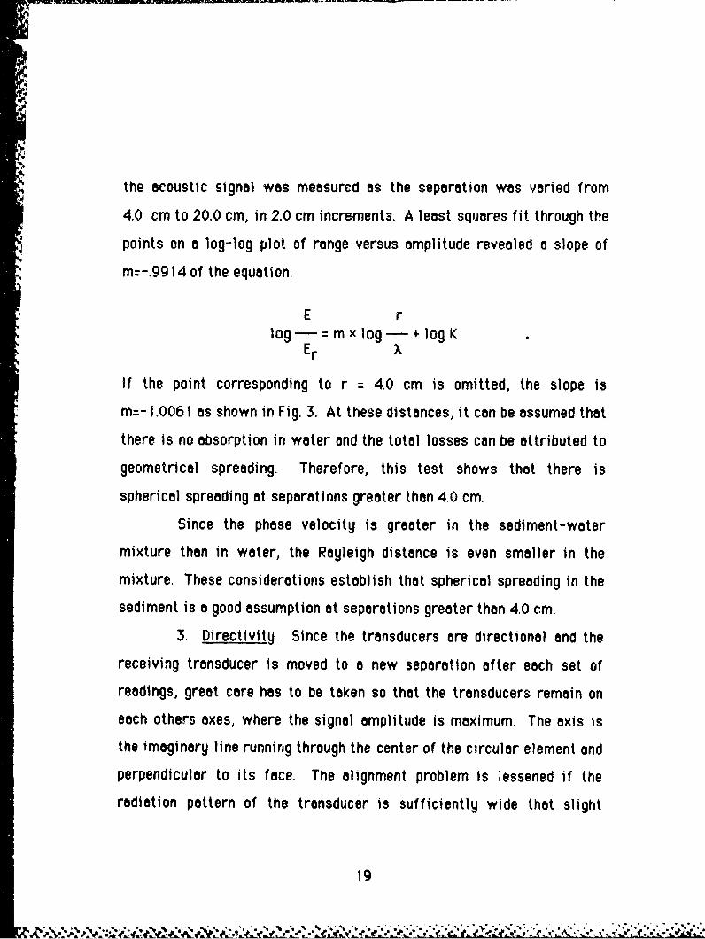
3. Directivity. Since the transducers are directional and the

receiving transducer is moved to a new separation after each set of

readings, great care has to be taken so that the transducers remain on

each others axes, where the signal amplitude is maximum. The axis is

the imaginary line running through the center of the circular element and

perpendicular to its face. The alignment problem is lessened if the

radiation pattern of the transducer is sufficiently wide that slight

19

II

FRESH WATER 105 kHz

4,1.0 0

0.8

0.6-

0.4- -1.006

2 3 4 5 6 7 8 9 10 20rT

." lg 'rE log L+ log K

! XKEr K'

0. 2I I II I I

Emg - ao-L+lo

r r

FIGURE 3SPHERICAL SPREADING IN FRESH WATER

ARL:UTAS-84-1035

20 DROcGA11-19-84

•...,,*.. , :.•. ... ,.,,., n'...,,*. *I, .. t't.,.,. ,.a..... ,:,.. -I,.* *. : .. ,: .- ,,.. *,,, ,,, *, '... ,.I,., .. ,,..,..,..•

errors in realigning the receiver exactly on the axis of the transmitter

will cause only slight error in measuring the on-axis signal amplitude.

By treating the transducer as a circular piston in an infinite,

rigid baffle, the half-power angle can be calculated. If p(O,r,t) is the on-

axis pressure, then the half-power angle is the angle at which the! pressure is given by (Blackstock)

*p(OHr,t) = p(O,r,t)/F/2

For a circular piston, the half-power angle is (Blackstock)

sin Oi =1.616/ka

In fresh water, at a frequency of 105.0 kHz, the calculated half-power

angle for these transducers is 22.60.

Figures 4 and 5 show the measured directivity of the two

transducers in fresh water. Again, it is seen that the model of the

transducer as a circular piston in a rigid baffle works well. The

directivity patterns for both transducers show that the half-power

angle, the angle at which the pressure is 3.0 dB below the on-axis

pressure, is about 200.

Since transducer I is used as the receiver in this experiment,

and is moved after each reading, it is desired that the response of this

transducer especially be constant for small angles off axis. This is so

that failure to exactly realign the transducers will still give a reliable

measurement of the on-axis value of the signal amplitude. Fig. 4 shows

that the sound pressure level, Lp. for transducer *1 varies less than

21

0'330*.• 30*

-10 HALF-POWER"POINTS ARE

S~CIRCLED

-

S2700 900

240" 120'

: 210* 150" •RANGE: 4.5 ft

FILTER: 50-200 kHz ISO* DEPTH: 3.0 ft"FREQUENCY: 105000 Hz TEMPERATURE: 21*C

FIGURE 4DIRECTIVITY PATTERN IN HORIZONTAL PLANE

FOR TRANSDUCER No. I IN FRESH WATER

I,;

22AS8-RDC -GA1-23-15

I0*

10 HALF-POWER/" POINTS ARE"° "----CIRCLED

.J2700 - 90°

/N

210* 150 *RANGE: 4.5 ft

FILTER: 50-200kHz 180° DEPTH: 3.0 ftFREQUENCY: 105000 Hz TEMPERATURE: 21"C

FIGURE 5DIRECTIVITY PATTERN IN HORIZONTAL PLANE

FOR TRANSDUCER No. 2 IN FRESH WATER

AFIL:UTAS-85-573RDC. GA

23 1-2-.• 6.

0.5 dB for 7.00 on either side of the axis. A 0.5 dB difference in L

implies that the actual pressure varies less than 6.0% from the on-axis

value. Actually, the L for transducer *1 is essentially constant for

angles up to 3.00 off axis.

For media such as saturated sediments, in which the sound

speed is higher than that of water, the half-power angle would be even

greater. A typical compressiona) wave speed for a sediment-watermixture is 1800 m/s (Bell, 1979). At the seme frequency that is being

considered, 105.0 kHz, this laads to a half-power angle of 280. Thus one

is led to believe that for small angles off axis, the signal amplitude

0would ary even less in the mixture than it would in water. In the

measurements taken in this investigation, it was estimated that the

receiver was positioned in the sediment with no more than 40 variation

in the angle off axis. Thus, there is confidence that the on-axis signal

amplitudes were measured accurately.

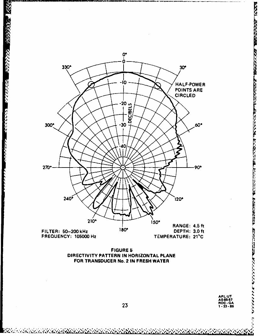
D. Sediment Preparation

The experimental sediment is made up of MS-MH size glass

beads manufactured by the Ferro Corporation of Jackson, Mississippi.

The grain size distribution is shown in Fig. 6 (Bell, 1979).

The sediment-water mixture was prepared in a five gallon,

plastic bucket in the following manner. The bucket is approximately

"35 cm high and 29 cm in diameter. The liquid in the sediment-water

mixture is circulated by a Masterflex tubing pump. Before the mixturewas put in the bucket, the outflow tube was attached to the bottom

24

80-

i60-

! -

80

LU40-

20

SIZE - mm 1.0 0.25 0.0625

FIGURE 6GRAIN SIZE DISTRIBUTION FOR MS-MH SIZE BEADS

25 ARL:UTAS-8558RDC- GA1-23-85

of the bucket with duct tape. The bucket was then partially filled with

de-ionized water and the input hose was put in the water. The pump was

turned on so that all of the air was driven from the tube. To retard the

growth of micro-organisms, 20 ml of BIO-CLEAN Ill algaecide was added

to the water.

The glass shot was then poured slowly into the water until the

sediment-water mixture was 24 cm deep. Pouring was halted at

intervals and the mixture kneaded to remove air trapped in the beads. A

layer of water, approximately 6 cm thick, was left on top of the

sediment mixture and the input hose to the pump was suspended in the

layer, as shown in Fig. 7. iThe bucket was then placed inside a vacuum tank on top of a

vibrator to remove any air remaining in the mixture. The tank was

evacuated and the mixture was vibrated in excess of 6 hours. The

mixture was left in the vacuum overnight, but the vibrator was turned

off. After the sediment was removed from the vacuum, the transducers

were inserted into the mixture so that the center of the elements were

12 cm below the sediment-water interface.

To alter the fluid properties, glycerine was poured into the

liquid on top of the mixture and the pump turned on until the liquio in the

bucket was well mixed. Approximately 10 ml of algaecide was added

while the liquid was being circulated to further retard the growth of

micro-organisms. The specific gravity of the liquid was measured

several times while the liquid was being circulated. The liquid was

considered well mixed after the values of specific gravity had stabilized.

26

29mc

FIUR 77CIRULTIN TE PREFLUID

.7 . . . .

.S855

PUMP~~D -. SEIMNA2c 1-2 -8

I �

.4

This usually occurred after about 3 hours. The specific gravity wasA

'4

II

measured using a hydrometer and the value of viscosity was determined

from a table containing values of viscosity for varying concentrations of Ngl�cerine-water solutions (Sheely, 1932).

pp1* 4

4*� '-'V4 5.4.

di.

p IIA

5�

'S

5,;

S.

r

I'a

.4

26

.4

\.'-�.-;�'�;: P�

IV. EXPERIMENTAL PROCEDURE

A. Phase Velocity

The oscilloscope trace is triggered at the beginning of the

transmitted four cycle pulse. The delay time to the fourth positive peak

on the received signal is measured with a digital readout on the

oscilloscope. This is first done at a transducer separation of

approximately 20 cm, and then at every 2.0 cm increment down to a

separation of 6 cm. If these delay times are then plotted on a time

versus distance graph, with time as the horizontal axis, the points

should fall on a straight line parallel to the characteristic of the

wavelet. The slope of this line is the phase velocity.

Therefore, to find the phase velocity a least squares routine is

used to fit the best straight line through these points. Since the line is

parallel to a characteristic, the equation of the line is of the form

r = cot + B

where co is the phase velocity, B is the intercept of the r-axis, and r and

t represent the separation and time delay, respectively. If the time were

measured from the fourth positive peak on the transmitted pulse to the

same peak on the received pulse, B would ideally be zero (for a

nondispersive medium) and the least squares line would be the same as

the characteristic. But since time is measured from the beginning of the

triggered pulse and there are additional time delays associated with the

circuitry and transducers, B turns out to be negative.

29

is

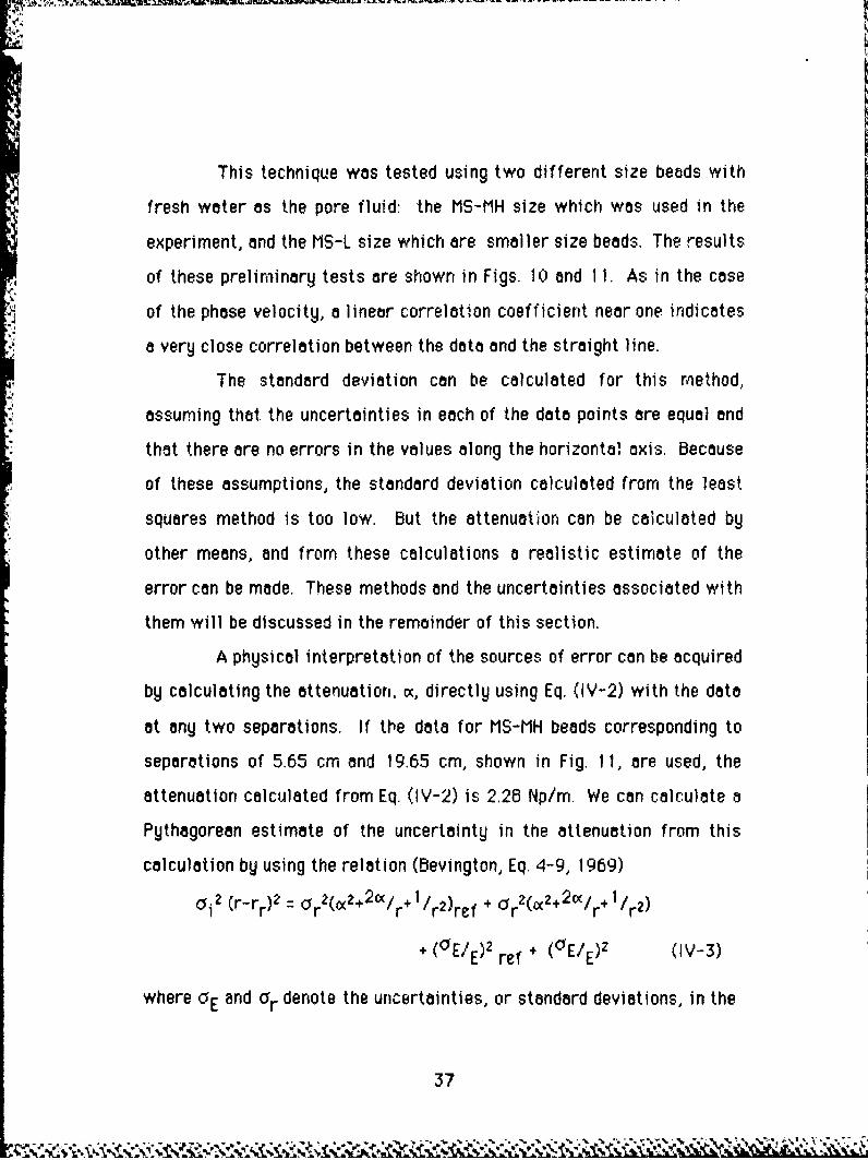
This method was tested using two different size beads with

fresh water as the pore fluid: the MS-MH size which war used in the

experiment, and the MS-L size which are smaller size beads. The results

of these preliminary tests are shown in Figs. 8 and 9. The linear

correlation coefficient displayed in the figures is a number between zero

and one that gives an indication of how well the data points fit a

straight line. A coefficient of one represents perfect linear correlation

and a coefficient of zero represents no correlation. The coefficients

shown in the figures indicate a very good correlation between the data

and the straight lines. The good correlation suggests that the

disturbances in the sediment, caused by moving the transducer to each

separation, have a negligible effect on the measurement

In order to check the validity of our procedure, we measured the

phase velocity in water at room temperature, approximately 250 C, six

times. Each of these results were between 1492 m/s and 1508 m/s. The

average of these measurements was 1501 m/s. By linear interpolation

of tabulated values of sound speed as a function of temperature (AIP

Handbook, 1963), the speed of sound at 250C in fresh water is 1496 m/s.

The average then has an error of only 0.33%, while the extreme values

have errors of -0.3% and 0.8%.

In another check, we compared our results to results obtained by

Bell (Bell, 1979), Shirley (Bedford, Appendix A, 1982), and Hovem and

Ingram (Hovem, 1979). We measured the phase velocity three separate

times in MS-MH beads with fresh water as the pore fluid. The three

results are shown in Table I, along with the other results mentioned.

30

BEAD TYPE: MS-MHFREQUENCY: 105kHz VISCOSITY: 0.893 cP

TIME - Is SEPARATION - cm

65.88 5.6577.63 7.6588.98 9.65

100.12 11.65112.07 13.65121.38 15.65133.23 17.65142.31 19.65

VELOCITY: 1820 m/sSTANDARD DEVIATION OF VELOCITY: 24 m/s

LINEAR CORRELATION COEFFICIENT: 0.9995

20- EXPERIMENTAL, DATA /18 - LEAST SQUARES FIT TO DATA

16-

E 14-

'12- /z0 ° /<8

w

4-

2

O " I I I - I!II1

0 20 40 60 80 100 120 140 160TIME -Mls

FIGURE 8PHASE VELOCITY IN MS-MH BEADS

31 ARL:UTAS-85-60RDC . GAI 23 • 85

BEAD TYPE: MS-LFREQUENCY: 105.0kHz VISCOSITY: 0.893 cP

TIME -,us SEPARATION - cm U63.62 4.6573.39 7.6583.49 9.6595.51 1 1÷65

107.15 13.65118,50 15.65131.73 17.65138.99 19.65

VELOCITY: 1791 m/sSTANDARD DEVIATION OF VELOCITY: 34 m/s

LINEAR CORRELATION COEFFICIENT: 0.9989

20 A EXPERIMENTAL DATA

18 LEAST SQUARES FIT TO DATA

16-14 -'••

12/z0 10

ch 6-/

4-

2-

0- I I0 20 40 60 80 100 120 140 160

TIME - us

FIGURE 9PHASE VELOCITY IN MS-L BEADS

32 ARL:UTAS.-5-61RDC - GA1 -23-85

I I .- -, *•` r* .=`•r` r."•• • ' * "1 I,• • 1 * . .. . •

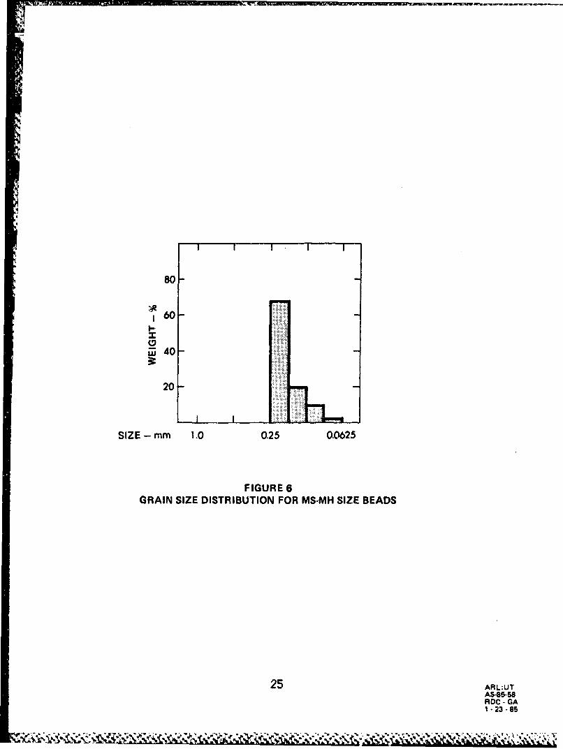
Comparison with these other results indicates that our results are valid.

But the comparison also suggests that the velocity is strongly dependent

on the depth of the transducers in the sediment.

The comparison in the MS-L size beads is not nearly so good.

Our first trial measurement in sediments was made in the MS-L size

beads. Since the standard deviation accompanying this measurement is

so large, 34 mis, and since in all subsequent measurements the standard

deviation was substantially reduced, the discrepancy is attributed to

experimental error and carelessness in precisely determining the

separation. As the experiment progressed, the technique improved and

the errcr decreased.

Table 1: Comparison of Velocity Results in MS-MH and MS-L Size Beads.

Frequency - kHz Depth - cm Velocity - m/s

MS-MH MS-L

Bell 120. 9 1809 18654

Shirley 114. 10 1808

Hovem & Ingram 100. 20 1922

Present Study 105. 12 1820 1791105. 12 1840105. 12 1866

33

• o • a . o ~*.a2. o o .L • o •

Obviously, the sound speed measurements in sediments are not

nearly as repeatable as the measurements made in water. One reason for

this is the uncertainty in the separation measurement. In the sediment,

this uncertainty is estimated to be 0. 1 cm. At a separation of 20 cm this

represents a relative uncertainty of 0.5 %, while at 6 cm the uncertainty

is 1.7%. The uncertainty in the time delay measurement is negligible

compared to this. Relative uncertainties of 0.5% and 1.7% in the

separation represent absolute uncertainties of 10 m/s and 30 m/s in the

velocity, respectively.

The standard deviations shown in Figs. 8 and 9 were derived

from the least squares method. In this calculation of the uncertainty it

was assumed that the uncertainties in the time delay measurements,

which were measured along the horizontal axis, were negligible. It was

also assumed that the absolute uncertainties of each of the separation

measurements, which were represented on the vertical axis, were equal.

Since both of these assumptions are appropriate and the standard

deviations calculated from the least squares method are consistent with

uncertainties in the separation measurements, these standard deviations

are a realistic measure of the uncertainty in the velocity.

All of the velocity measurements made in the sediments are

listed in Table VII of Chapter IV and in Appendix B together with the raw

data. It can be seen that the standard deviations of the velocities were

less than 15 m/s after the first few trial measurements. This indicates

that as the experiment progressed, the technique was improved and the

uncertainty decreased.

34

S-.. . _ . . . . . .. . . .. .

i:• B. Attenuation

:i 1. Measurement Technique. In the sediment the losses are due toibothgeometricalspreadingandabsorptionofthemedium. Therefore, to

,.. calculate the attenuation by the medium the geometrical spreading must-be taken into account. As discussed in Section III.C.2., the transducers

were designed so that the Rayleigh distance would be relatively small

compared to the sediment sample. At distances greater then the

Rayleigh distance, the signal amplitude decays as 1/r due to spherical

spreading, where r is the separation between the transducers. This

distance was calculated for both water and the sediment. The

calculation for water was then verified by acoustic measurements.

These measurements support the calculated assumption that the

geometrical spreading in the sediment is indeed spherical at the

distances at which the attenuation measurements are taken. Using

spherical spreading, the losses due to absorption in the sediment can be

determined. A detailed discussion of this procedure follows.

TThe measurements establishing the llr decay of the signal

amplitude due to spherical spreading have been discussed inSection III.C.2. We determine the absorption due t the mencium bye

measuring the amplitude of the signal and assuming that the amplitude

varies as

E = (K/r) e-or (IV- 1)

in an absorbing medium. Here, K is a calibration constant with units of IN

voltsxlength and o( is the attenuation in nepers per unit length. The 1/r

factor in Eq. (tV-i) takes into account the sphericl spreading and the

3517

OW'.

eCur term takes into account the absorption of the medium. It is also

assumed that the coupling between the sediment and the transducer is

the same at each separation. Thus, the decay in amplitude of the signal

is attributed only to the increase in separation.

The attenuation is determined by comparing the amplitudes

measured at various separations. To do this, one of the amplitude

measurements and the separation at which it is measured are designated

as reference values, E and r, respectively. In this experiment, rr is

the smallest separation at which measurements are taken and Er E at

r = rr. Therefore the following relation holds:

Er =(K/ rr e-crr

From this and Eq. (IV. 1) it follows that

K = IEr e°cr = Er rr earr

ec(rrr) = Er rr/(E r)

ot(r-rr) I in [Er rr/(E r)] . (IV-2)

Therefore, if Wn[Errr/(E r)) is plotted versus (r-rr), the points should fallr ..

on a straight line and the slope of this line is the attenuation To find the

slope of this line, and thereby the attenuation, the method of least

squares can again be employed. I36

. .. .,7x.y,,. , , ,. ., .. ... .. . .. . . . . . ..%

-. -" • , • .'' . ,', '- '-' .'' ".- 9, ", "• .-. "-. ' -.- .' t: -•'...''.-. A" .',' ' ' '. .•, ,:," •:. ,; ,,, '; -

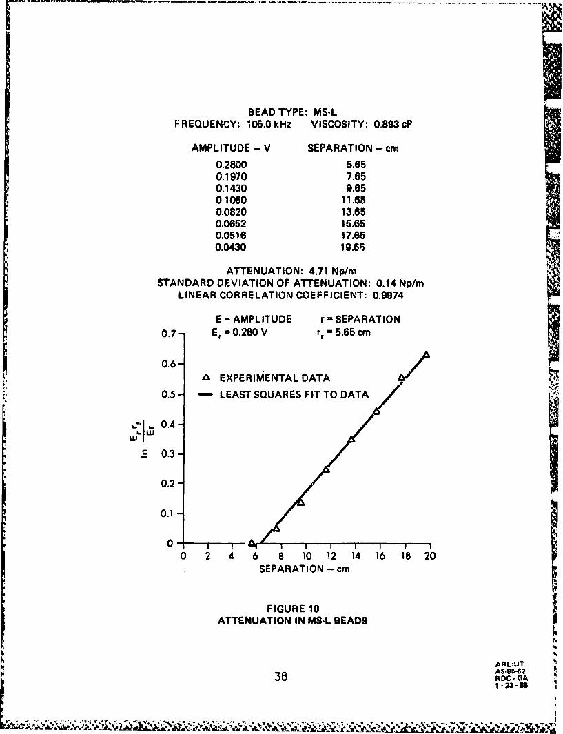
This technique was tested using two different size beads with

fresh water as the pore fluid: the MS-MH size which was used in the

experiment, and the MS-L size which are smaller size beads. The results

of these preliminary tests are shown in Figs. 10 and 11. As in the case

of the phase velocity, a linear correlation coefficient near one indicates

a very close correlation between the data and the straight line.

The standard deviation can be calculated for this method,

assuming that. the uncertainties in each of the data points are equal and

that there are no errors in the values along the horizontal axis. Because

of these assumptions, the standard deviation calculated from the least

squares method is too low. But the attenuation can be calculated by

other means, and from these calculations a realistic estimate of the

error can be made. These methods and the uncertainties associated with

them will be discussed in the remainder of this section.

A physical interpretation of the sources of error can be acquired

by calculating the attenuation, cK, directly using Eq. (IV-2) with the data

at any two separations. If the data for MS-MH beads corresponding to

separations of 5.65 cm and 19.65 cm, shown in Fig. 11, are used, the

attenuation calculated from Eq. (IV-2) is 2.28 Np/m. We can calculate a

Pythagorean estimate of the uncertainty in the attenuation from this

calculation by using the relation (Bevington, Eq. 4-9, 1969)

di2 (r-rr)2 = fr (+2(xI/r+ /1r2)ref + •r( 1 /r2)

+ (E/E )2 ref + (0 E/E)2 (IV-3)

where -5E and orr denote the uncertainties, or standard deviations, in the

37

BEAD TYPE: MS-LFREQUENCY: 105.0kHz VISCOSITY: 0.893 cP

AMPLITUDE - V SEPARATION - cm

0.2800 5.650.1970 7.650.1430 9.650.1060 11.650.0820 13.650.0652 15.650.0516 17.650.0430 19.65

ATTENUATION: 4.71 Np/mrSTANDARD DEVIATION OF ATTENUATION: 0.14 Np/m

LINEAR CORRELATION COEFFICIENT: 0.9974

E - AMPLITUDE r - SEPARATION

0.7- Er 0.280 V rr = 5.65 cm

0.6-AEXPERIMENTAL DATA

0.5- LEAST SQUARES FIT TO DATA

0.4-

S 0.3-

0.2-

0.1-

0-2 4 6 8 10 12 14 16 8 20

SEPARATION - cm

FIGURE 10ATTENUATION IN MS-L BEADS

S~ARL:UTAS-85-6238 ADC-6Aii~1 - 23 -85

BEAD TYPE: MF)-MHFREQUENCY: 105.0 kHz VISCOSITY: 0.893cP

AMPLITUDE - V SEPARATION - cm

0.3720 5.650.2690 7.650.2004 9.650.1570 11.650.1300 13.650.1074 15.650.0892 17.650.0777 19.65

ATTENUATION: 2.40 Np/mSTANDARD DEVIATION OF ATTENUATION: 0.09 Np/m

LINEAR CORRELATION COEFFICIENT: 0.9962

0.4 E = AMPLITUDE r - SEPARATION

Er = 0.3720 V rr = 5.65 cm

0 EXPERIMENTAL DATA

LEAST SQUARES FIT TO DATA

ujI 0.2-

0.1-

0 7-0 2 4 6 8 10 12 14 16 18 20

SEPARATION - cm

FIGURE 11ATTENUATION IN MS-MH BEADS

ARL:UTAS85-63RDC. GA

39 1.23.85

"'k '

amplitude and separation, respectively, and the quantities marked "ref"

signify that the separations and amplitudes correspond to the separation

of 5.65 cm. To perform this calculation, the uncertainties in the

separation and the amplitude, 0 r and CE, must first be determined. The

uncertainty in the separation is estimated to be 0.1 cm.

The uncertainty in the amplitude has two sources. The first one

is instrumental, because the oscilloscope can be read accurately to 1/4

of a gradation. The scale is changed at different separations, since theV

amplitude grows with decreasing r, so this type of uncertainty increases

with decreasing separation.

The second source of uncertainty in E is due to the uncertainty

in r. Since the amplitude is a function of r, as was assumed in Eq. (IV-I)..

any uncertainty in r produces an uncertainty in E. This type of error can

be estimated from the relation (Bevington, Eq. 4-9, 1969)

CE = ar El r r E ( oar + Ir)

By calculating this uncertainty, and comparing the results with thie

instrumental uncertainty in E, it can be seen that over 80% of the

uncertainty in E is due to the uncertainty in r. Using Eq. (IV-3), and the

values in the rows in Table II corresponding to r=19.65 cm and r=5.65 cm,

the uncertainty in the direct calculation is found to be 0.522 Np/rn. Note

from Eq. (3) that the uncertainty, ai, is inversely proportional to the

difference between the two separations being compared. Thus, one way

to improve the measurements would be to increase the distances over

which the measurements are taken.

40

Using each pair of data shown in Fig. 1I, the attenuation can be

calculated seven times In this way, and the values designated as 0(i.

These seven values of attenuation can then be weighted with their

corresponding uncertainties, ai, and averaged as shown in Table II

(Bevlngton, p. 73, 1969). The resulting average is a better estimate of

the attenuation than any of the individual attenuations, and the standard

deviation calculated from this method Is a better estimate of the

uncertainty. Although this value of x differs by 5% from the least

squares value, this standard deviation is a more realistic estimate of the

uncertainty.

"lable II: Analysis of Errors in Attenuation.

r - cm E - volts aE/E rrI(o•+ 2 cK/r+ 1 /r2) ci - Np/m cn i -Np/rn

5.65 0.372 0.0380 0.0004047.65 0.269 0.0407 0.000239 3.06 1.0579.65 0.2004 0.0460 0.000163 1.606 2.082

11.65 0.157 0.0429 0.000121 1.029 2.31713.65 0.130 0.0478 0.000095 0.813 2.11615.65 0.1074 0.0533 0.000077 0.690 2.23517.65 0.0892 0.0592 0.000065 0.613 2.40819.65 0.0777 0.0587 0.000056 0.522 2.283

oCK2 - so that C = 0.296 Np/mS('/oiy L

X = O2 (xi/cri2) = 2.266 Np/m

41

NW411

In calculating the attenuation using this method, the error in the

reference separation and amplitude is repeated in each of the seven

calculations. Thus, it reference measurements are particularly bad, the

error in them will be compounded in the final result. To avoid this type

of error, the attenuation can be calculated with any two pairs of data, E

and r. The values corresponding to r = 5.65 cm do not necessarily need to

be the reference separation and amplitude. Since there are eight pairs of

data, there are 28 possible ways to calculate (x using Eq. (IV-2). TheN 'unweighted mean of these 28 attenuations and the standard deviation of

this mean can be easily calculated. For the MS-MH beads of Fig. 11, this

mean is cK = 2.38 Np/m and the standard deviation is F• = 0.47 Np/m.

This value of the attenuation differs only by 0.6% from the least squares

value. But this standard deviation is larger than the one calculated from

the weighted averages. This may signify that the estimate of the

uncertainty in r used in that calculation, rr = 0.1 cm, was too low. In

later calculations, however, there is better agreement between these

two calculations of the sttndard deviation. This suggests that the

separation was determined more precisely as the experiment progressed.

Another reason for the discrepancy is that all of the attenuations are

weighted equally in calculating the mean. But as can be seen from

Eq. (IV-3), the uncertainty decreases as the difference between the two

separations increases. Thus, the standard deviation calculated by this

method represents an upper bound of the actual uncertainty in the

attenuation.

42

The attenuation was calculated for each value of viscosity usingthe method of least squares and the mean of all combinations. In each

case, the two values of attenuation differed by less than I%. But we feel

that the standard deviation associated with the mean of all combinations

was more realistic.

It can be noted that the uncertainty in the separation is by far

the biggest source of error. Therefore, to improve these measurements,

a method for determining the separation of the transducers more

accurately would have to be devised. Toward this end, the separations

were corrected using the velocity results. The attenuations were then

calculated by the mean of all combinations with these corrected

separations. These attenuations were within 1% of the attenuations

calculated by the other methods, except for the case of the MS-MIH beads

of Fig. II where the difference was 2.5%. In all but a few cases, the

standard deviation was substantially reduced. Thus, the attenuation was

calculated by the mean of all combinations. In all but those few ceses

where the standard deviation was not reduced, the separations were

corrected using the velocity results. Reducing the data in this way, we

are confident that the attenuations were determined within 3 dB/m,

except for a few cases. The attenuations and their uncertainties,

corresponding to each fluid viscosity, are listed in Table VII in

Chapter IV. They are also listed together with the rew data in

Appendix B.

43

,.• L•

2. Co__parison of Results. To determine the validity of the

attenuation results, the measurements in the water saturated beads,

with no glycerine added, were compared to the results of David Bell

(Bell, 1979). His attenuation measurements were given in decibels per

wavelength. Converting his results to nepers per meter at 105.0 kHz

resulted in the values of 5.45 Np/m and 3.13 Np/m for MS-L and MS-MH

size beads, respectively.

The discrepancy in attenuation between Bell's values and those

presented in Figs. 10 and 11 was 0.74 Np/m in the first case and

0.73 Np/m in the second. Since this difference was too large to be

attributed to experimental error, an effort was made to explain it.

In order to account for the geometrical spreading of the

tranisducers, Bell measured the amplitude decay in water at 120 kHz and

the amplitude decay in the sediment at the some frequency. He assumed

that the only losses in the water were due to geometrical spreading and

that the losses in the sediment were due to geometrical spreading and

absorption in the medium. He then assumed that the losses due to

°* geometrical spreading in the sediment were the same as in water, at the

some frequency. Therefore, to calcuiate the attenuation he subtracted

the spreading losses, which he determined from his measurements in

water, from the total losses (Bell, 1979).

In doing this, he assumed that the geometrical spreading in the

water was the same as in the sediment, for measurements taken at the

same frequeocy. But the Rayleigh distance, which is a measure of the

distance at which spherical spreading starts, is inversely proportional to

the sound speed. Since the sound speed is greater in the sediment than in

44

the water, the Rayleigh distance is smaller in the sediment than in the

water. Also, the distances at which he took his measurements were less

than the Rayleigh distance for his transducers, so that in water his

amplitude did not vary as I/r. Therefore, the losses due to geometrical

spreading were less in the water than in the sediment. The extra

geometrical spreading that was occurring in the sediment was attributed

to absorption in the sediment, resulting in a value of attenuation that

was too large.

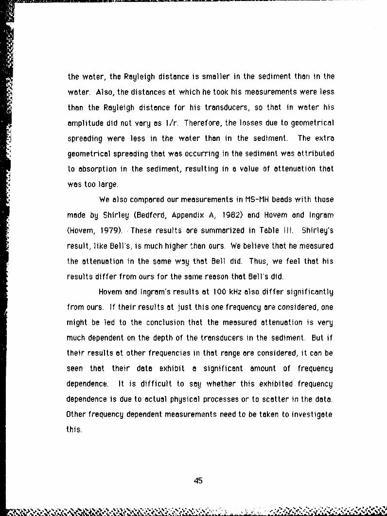
We also compared our measurements in MS-MH beads with those

made by Shirley (Bedford, Appendix A, 1982) and Hovem and Ingram

(Hovem, 1979). These results are summarized in Table 11. Shirley's

result, like Bell's, is much higher than ours. We believe that he measured

the attenuation in the same w~y that Bell did. Thus, we feel that his

results differ from ours for the same reason that Bell's did.

Hovem and Ingramis results at 100 kHz also differ significantly

from ours. If their results at just this one frequency are considered, one

might be led to the conclusion that the measured attenuation is very

much dependent on the depth of the! transducers in the sediment. But if

their results at other frequencies in that range are considered, it can be

seen that their data exhibit a significant amount of frequency

dependence. It is difficult to say whether this exhibited frequency

dependence is due to actual physical processes or to scatter in the data.

Other frequency dependent measurements need to be taken to investigate

this.

45

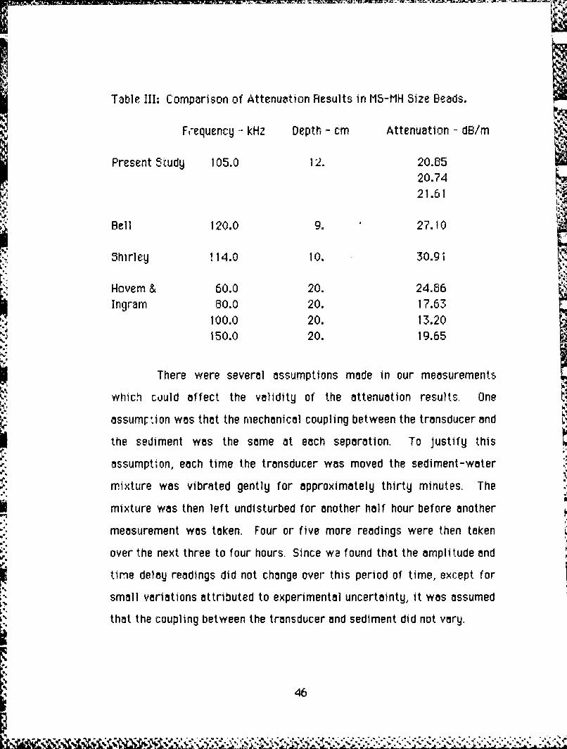
Table III: Comparison of Attenuation Results in MS-MH Size Beads. I.,,Fr-equency - kHz Depth - cm Attenuation - dB/m

Present Study 105.0 12. 20.8520.7421.61

Bell 120.0 9. 27.10

Shirley 114.0 10. 30.9i

Hoverm & 60.0 20. 24.86Ingram 60.0 20. 17.63

100.0 20. 13.20

150.0 20. 19.65

There were several assumptions made in our measurements

which could affect the validity of the attenuation results. One

assumFpion was that the mechanical coupling between the transducer and

the sediment was the same at each separation. To justify this

assumption, each time the transducer was moved the sediment-water

mixture was vibrated gently for approximately thirty minutes. The

mixture was then left undisturbed for another half hour before another

measurement was taken. Four or five more readings were then taken

over the next three to four hours. Since we found that the amplitude and

time delay readings did not change over this period of time, except for

small variations attributed to experimental uncertainty, it was assumed

that the coupling between the transducer and sediment did not vary.

46

3. Transient Considerations. From a theoretical viewpoint, it

would be desirable to measure the time delay and amplitude using a

steady state signal. In this way, we could be confident that the signal

had a single frequency. The transient characteristics of the transducers

could also be neglected. However, the container holding the sediment has

a a limited volume. Thus, there will be reflections of the signal from the

sides of the container and from the sediment-water interface. To

prevent these reflections from interfering with the signal that travels

along the direct path between the two transducers, a four cycle pulse

was transmitted. The signal was then cut off for several milliseconds

so that all the reflections in the sediment would attenuate before a new

pulse was transmitted. A photograph of the oscilloscope trace of the

transmitted and received signals is shown in Fig. 12. Note that the

received signal contains more than four cycles. Since the transducers

are being operated at one of their resonant frequencies, they continue to

vibrate, or ring, for several cycles after the input signal is turned off.

In this section and the next, an attempt is made to justify

treating the pulses as steady state, harmonic signals in analyzing the

data and comparing it to the theory. This section discusses the transient

effects of the transducers on the signal amplitude. The signal amplitude

can also be affected by dispersion. These effects are discussed in the

next section.

Since we compared amplitude measurements at different

separations to calculate the attenuation, it is assumed that the

measured voltage amplitude is linearly proportional to the acoustic

47

*E(1 U1 a

VI __=C'E 0(w (a)

(b)

HORIZONTAL SCALE: 20ps/DIV

VERTICAL SCALE:(a) RECEIVED SIGNAL - 0.05 V/DIV(b) TRANSMITTED SIGNAL- 5 V/DIV

SEPARATION: 8.04 cm

FIGURE 12

*" TRANSMITTING AND RECEIVING PULSES IN SEDIMENTS

ARL:UT48 AS-8.5259DRC - GA

3•13 -85

pressure amplitude that produced it in the sediment. In order to justify

this assumption, consider the block diagram in Fig. 13. The amplitude of

the voltage signal put in to the transmitter is denoted by Ei. This

produces an acceleration of the transducer face, denoted by u. The signal

produced by this motion of the transducer face travels a distance r to the

receiver., where it produces a pressure P0 . The receiver converts this

pressure signal to an output voltage signal E0. The phase constant

signifies that the measurements are taken on the fourth cycle. Thus

Eo(+), shown in Fig. 12, represents the peak-to-peak, voltage amplitude

of the fourth cycle of the received signal. The operators L 1, L2 , and L

denote linear functions of their arguments.

Our use of the phase constant + deserves some explanation. If T

represents the period of one cycle, then the positive and negative peaks

of the fourth cycle will correspond to the phases

=t+ - r/co = 3.25 T

and =t_ - r/co = 3.75 T

respectively. Note that the separation r is the same in each case, so that

the difference in the travel times t+ and t- is 0.5T. The pressure

amplitude of the fourth cycle is then

Pore = Po(p- Po0(+).

Since u represents the acceleration of the transducer face, and the phase

represented by 4 spans half of a period, the quantity u(+) does not really

49.4

49 "'

r,

TRANSDUCER IMENT TRANSDUCER

u(o) = 1(Ei(O)) P0(0) =K e'•u (0) £01€) =L(P()

"FIGURE 13LINEARITY OF THE TRANSDUCERS

ARL:IJT50 AS-5-260

DRC - GA3 -13 -85

make sense. But in Fig. 13 it represents the quantity

u(+) = U(+4 - U(+-)

The terms Eo(4) and Ei(+) have similar meanings.

Consider the two graphs of EIo() versus Ei(1) shown in Fig. 14.

These were taken by varying the amplitude of the input voltage, Ei(+),

and measuring the amplitude of the fourth cycle of the output voltage

signal. The graphs were made at the distances r = 10.0 crn and

r = 20.0 cm so that the entire range of received amplitudes that were

measured in the experiment would be covered. The graphs show that the

output amplitude of the fourth cycle, Eo(4), is a linear function of the

input amplitude Ei. This can be expressed as

Eo(+) = L3 (Ei(+))

To calculate the attenuation, it is assumed that the pressure

signal decays according to

Po(r,t) = (Klr) e`'•r u(t-r/ c.)

where K represents an arbitrary constant, and co is the phase velocity.

The axial, farfield pressure due to a transient signal in a nonabsorbing,

nondispersive medium is

Po(r,t) = (K/r) u(t-r/CO)

To account for the attenuation, the exponential term was incorporated,

ad hoc. Taking the attenuation into account in this way is justified

because the farfield pressure on the axis for steady state, harmonic

51

VS

F

0.12wa -

INPUT AMPLITUDE-V

(a) LINEAR AMPLITUDE RELATIONSHIP AT 20 cm

'" ~0.4- •

Jl 0.08

-0.2

C0o.1

0.

0 -4

0 2 4 6 8 10 12 14 16INPUT AMPLITUDE V

(b) LINEAR AMPLITUDE RELATIONSHIP AT 10 cm

FIGURE 14INPUT VOLTAGE AMPLITUDE versus OUTPUT VOLTAGE

AMPLITUDE OF THE FOURTH CYCLE

ARL:UT52 AS-85-26152 DRC - GA

3 -13 -85

II

radiation from a baffled piston is given by (Blackstock)

Po(,t) = (K/r) ei(wt-kr)

The e-c~r term is arrived at in this case by assuming that the wave

number k is complex, where (x Is its imaginary part. Since u(+') is a

Sconstant, we get

PO(+) =(K/r) e-or

Therefore, the assumption used to determine the attenuation,

Eo(>) = K/r e-cr (I)

will be valid if Eo(4) = L2 (Po(#)) . (2)

To show that (1) is valid, assume that (2) is true and also that

u(+) = L I(Ei(+))

This is the same as assuming that the transducers produce a signal

amplitude that is linearly proportional to their signal input, for a given

cycle. it therefore follows that:

Eo(+) = L2(Po(+))

"= L2 [(K/r) e-xr U(+)]

"= (K/r) eCr L2(u0<))

"= (K/r) eor L2{L1[E1(4)])

"=(Klr) -Car L,[Ei(<+)]

" (K'/r) e-c<r Ei (+))

where K' is another arbitrary constant. For a fixed r, this shows that

Eo(4) is linearly proportional to Ei(4), which has been demonstrated in

53

ALI

the two graphs of Fig. 14. This result supports the assumption (2).

Furthermore, Ei(4) is a constant so that (1) directly follows.

4. Effects of Dispersion. In determining the attenuation, the

decrease in amplitude with increasing separation was attributed to two

causes; spherical spreading and absorption of the medium. In reducing

the data, it was assumed that the signal contained only one frequency

and that any dispersion could be neglected. But, since the transmitted

signal was the product of a sine wave and the difference between two

step functions, the signal contained a continuum of frequencies. We

justified treating the signal as a pure tone by channeling the signal

through a narrow bandpass filter and by making our measurements on the

fourth cycle of the signal to minimize transient effects.

Since the signal did contain more than one frequency, dispersion

would cause a decrease in amplitude with increasing separation.

However, we believe that the effect of dispersion on our measurements

is very small. The theory and the measurements predict little change in

the phase velocity of the compressional wave of the first type with

frequency. Since the received signal is filtered as a further precaution,

we would expect the influence of dispersion on the amplitude to be

negligible.

To be more confident in this assumption, the attenuation was

determined by measuring the amplitudes from three consecutive cycles

on the received signal: the third, fourth, and fifth cycles. This was done

for three different sets of measurements. The results are shown in

Table IV. In each set, the three attenuations are within a standard

54

"4?S

deviation. The attenuation of the middle set exhibits the most spread,

* but even so the spread is still within the estimated uncertainties.

Curiously, the standard deviations corresponding to this set are the

smallest in the table.

If dispersion was a significant factor, the envelope of the

received signal would change shape as the signal propagated through the

sediment. This would cause the attenuations measured from amplitudes

*• of different cycles to be distinctly different. Since they are not, we

conclude that any error in the attenuation caused by dispersion is

negligible within the limits of error of our measuring technique.

Table IV: Comparison of Attenuations and Standard Deviations

Measured from Different Cycles of the Same Received Signal.

CYCLE VISCOSITY -cP ATTEN - dB/m STD DEV - dB/m

3 1.33 20.5 3.54 20.4 2.95 19.5 3.4

3 1.33 20.7 1.74 19.0 1.95 18.1 2.7

3 2.59 23.6 2.64 23.2 2.15 23.5 2.4

55

V. EXPERIMENTAL RESULTS

A. Pehysical Properties of the Sediment

In order to calculate the wave number using the theory outlined

in Chapter II, the physical properties of the saturated sediment needed to

be determined. The values of most of these parameters were easily

obtained, either by direct measurement or from tables listing material

properties, which were found in handbooks and journal articles.

Assigning numerical values to some of the other parameters, on the other

hand, was not so straightforward.

The physical properties of the solid and fluid constituents were Ithe most easily determined. Glass beads consttute the solid part of the

mixture. The density and bulk modulus of glass were found in several

sources (Bedford, 1982; Kinsler, 1982). The average grain size, or bead

diameter, was measured by Bell from a grain size analysis. The porosity

of MS-IH size beads was also determined by Bell (Bell, 1979). These

values are listed in Table V.

The properties of the fluid change in the experiment since IV

glycerine is added to the mixture after each set of measurements. The

density of the fluid is easily determined by measuring the specific

gravity with a hydrometer. Knowing the specific gravity and the

temperature, the viscosity was read from a table containing values of

viscosity for solutions of varying glycerine-water concentrations

(Sheely, 1932). Shirley measured the sound speed in glycerine-water

56

L~• " " ".• i' ':" ,•. - " " - ' • " " ." '• • • " . . . . " " • : - • .. . -

Table V: Physical Properties and Parameters of 8ediment Used inTheoretical Calculations.

PRESENTPARAMETER SYMBOL STUDY BEDFORD SHIRLEY

Porosity 4) 0.365 0.365 0.365

Bead Diameter (cm) dm 0.0177 0.018 0.0177

t Glass BulkModulus (x 10" dyn/cm2) Ks 3.9 4.07 3.5

Gloss Density (g/cm3 ) Ps 2.5 2.5 2.5

Frame BulkMiodulus (dyn/cm2) Kb 8.Ox I OF 5.8x 109 8.ox i or

Frame ShearModulus (dyn/cm2) .b 8.Ox I OT 5.8 103 B.Ox 107

Comp. Log Decrement sc 0.1 0.15 0.1

Shear Log Decrement 6s 0. 1 0. 15 0.1

Permeability (x10-? cm 2 ) B0 3.8 2.48 2.b4

Kozeny-Carman Constant ko 2.76 4.23 3.98

Depth in Sediment (cm) 12 20 10

57

solutions with varying concentrations of glycerine (Bedford, Appendix A,

1982). From this data, and values of density and viscosity at 20"C found

in the CRC Handbook, he was able to determine the bulk modulus as a

function of viscosity for concentrations up to 32% glycerine, by weight.

But since his measurements were taken at room temperature, which is

closer to 250C, we adjusted his measurements so that the bulk modulus

values corresponded to viscosity values at 250C. His results were then

projected to include glycerine concentrations up to 40%. The results of

this procedure are shown in Table VI. This extrapolation of his data is

questionable at best, but there was not enough time to repeat the

measurements. These adjustments produce only slight changes in the

theoretical predictions. At some point in the future it would be

desirable to redo and hopefully repeat Shirley's measurements.

The properties of the solid matrix are more difficult to

determine. With all of the other properties defined, these propertie.s

were chosen so that the theoretical predictions and the experimental

data agreed for the case of pure water. Once this agreement was

satisfied, we were able to show that the Biot-Stoll theory predicted the

same change in attenuation and phase velocity that was indicated by the

experimental data as the viscosity of the pore fluid was increase]J.

Four of these properties were the real and imaginary ,parts ofthe bulk and shear moduli of the drained glass beads. Hovem and Ingram

(Hoyem, 1979),. Shirley (Bedford, Appendix A, 1982), and Bedford(Bedford, 1984) chose the real parts of both of these moduli so that

thero was agreement between the theory and compressionol velocity

56

Table VI: Physical Properties of Fluid Used in Theoretical Calculations.

VISCOSITY FLUID DENSITY FLUID BULK MODULUST• - cP pf - g/cm 3 Kf - x1010 dyn/cm2

0.893 0.9971 2.1751.0 1.0080 2.2841.2 1.0242 2.4421.4 1.0373 2.5741.6 1.0453 2.6831.8 1.0576 2.7812.0 1.0654 2.8672.2 1.0723 2.9432.4 1.0785 3.0122.6 1.0840 3.0752.8 1.08867 3.128

59

Udata. Bedford made theoretical comparisons with Hovem and Ingram's

data and his choices of the parameters are very similar to Hovem andIngram's.

Bedford had good agreement between theory and data for

Kb = i-b = 5.8 x I09 dyn/m 2

But Hovem and Ingram's measured compressional velocity at 100 kHz,

1922 m/s, is considerably higher than ours for the pure water case,

1630 m/s. This is presumably because their measurements were made 8

cm deeper in the sediment than ours were. As a result, their choice of Kb

and Ob produced theoretical velocities that were too large for our data.

But the theoretical attenuations produced by this choice compared well

with our data. Shirley's measured velocity, at 114 kHz with pure wtiter

as the pore fluid, agreed quite well with our results. It should be noted

that our measurements were taken at similar depths. His choice for the

two moduli wasIIKb = b = 8. 10? dyn/cm 2

This choice produced theoretical velocities that agreed quite well with

our data. The disparity between these two sets of values suggests that

the properties of the sediment change drastically with increasing depth

in the sediment.

We used Shirley's values for the bulk and shear moduli, even

though the theoretical attenuations they produced were much too high.

This discrepancy, whicn was the result of differences in experimental

technique and data reduction, was discussed in Section IV.B.2. In order

60

to achieve a good fit between the theory and the experimental data for

the attenuation case, we had to choose other parameters differently

from Shirley.

The imaginary parts of the bulk and shear moduli of the granular

matrix are the terms that take into account the losses at the

grain-to-grain contacts. From our experience, these parameters have

negligible effect on the compressional velocity, and only a slight effect

on the attenuation. In the literature, these two parameters have been

related to their real counterparts by two other parameters, the

compressional and shear logarithmic decrements, Sc and S , respectively.

The relationships defining these parameters are

Kb = c Kbl! and b' b/11

where a primed variable denotes the imaginary part of the modulus and

an unprirmed varible denotes the real part. Our choices of these variables

are listed in Table V.The last parameter to be chosen was the permeability. Bell

measured this quantity directly for four sizes of glass beads and three

different sands (Bell, 1979). For the MS-MH size beads he measured thepermeability to be B0 1.70 x 10- cm2 . The permeabilty is related to

an empirical parameter, the Kozeny-Carman constant, ko, by the relation

(Bell, 1979)

dmi2 +3

36 ko ( 1)Z

61

•_ :" "• 'd •• * ,• " '•• "• • • % ' " "% ' • '•• •% " °. . ,•• O ,, -

Bell's value for Bo corresponded to ko 6.17. Hovem and Ingram chose

ka= 4.23 so that BO = 2.48 x 10 -7 cm 2. Shirley used ko = 3.98 so that

Bo = 2.64 x 10 -c Cm 2. We found good correlation between theory and

data by choosing Bo = 3.7 x 10 -? cm 2 This corresponded to ko = 2.83.

This was within the range of values in the data presented by Stoll (Stoll,

1974) and also within the range of values measured by Bell for several

sands and sizes of glass beads.

Table V summarizes the values of the physical properties and

parameters used in the present study, and also those chosen by Bedford

(Bedford, 1984) and Shirley (Bedford, Appendix A, 1982). In Fig. 15 our

data are compared with the theory with Bedford's, Shirley's, and our

choices of the parameters.

'p

"4,

62

2200- do

jaw

2100 ,

"- /2000Sooo /

, .> e ll,,.) ,A 0 +O- DATA

1900- THEORY FROM PRESENT STUDY

0 --- THEORY FROM BEDFORD

1800- *....... THEORY FROM SHIRLEY

1 2 3VISCOSITY - cP

(a) PHASE VELOCITY

40 K

1 30-z

'z20- &.o-o0 -, ,A A

10

1 2 3VISCOSITY - cP

(b) ATTENUATION

FIGURE 15

COMPARISON OF BlOT THEORY TO DATA

ARL:UTAS-85-337DRC - GA

63 3-28-85

.• i -, • - - • • + -o • o - - . . .6 3-•

.

42.,:.. -, ..• , .. . . . . . . . . . . . . .

Table VII: Velocity and Attenuation in MS-MH Beads withVariable Fluid Properties.

VISCOSITY VELOCITY STD. DEV. ATTENUATION STD. DEV11 - cP co - m/sec Cc - M/sec o• - dB/m Crf -dB/m

BATCH I0.89 1820.0 23.6 20.7 4.10.89 1869.7 9.0 20.7 1.11.07 1861.3 6.8 21.3 2.21M22 1878.9 2.6 21.0 3.11.33 1893.3 4.2 20.4 2.91.33 1896.6 5.7 19.0 1.9

BATCH 20.89 1839.4 15.2 21.7 2.51.15 1873.8 8.7 23.1 2.2

1.48 1966.7 9.4 26.0 3.61.74 1973.3 6.9 20.9 2.82.16 2044.1 7.3 21.0 1.72.59 2067.5 9.2 23.2 2.12.81 2074.5 13.0 24.3 1.43.23 2098.8 12.1 24.3 2.2

DILUTING BATCH 22.46 2034.7 8.2 26.0 1.72.09 1986.6 3.6 20.8 1.6

64

repeatability of the results. The results for the three cases agree

reasonably well with each other and also with the theoretical curves.

The figures demonstrate that these experimental results are repeatable

within the estimated uncertainties, especially in the phase velocity

case. The larger amount of scutter, and the larger uncertainties, in the

attenuation results suggest that further improvements can be made in

that measurement technique. One suggestion would be to design m

bracket that would hold the transducer mount and guide it straight into

the sediment while it was being repositioned. This would probably be

the easiest and least expensive wey to reduce the most significant cause

of experimental error, that due to uncertainty in the separation

measurements.

The sediment is disturbed each time a transducer is

repositioned to take travel time and amplitude measurements at a new

separation. It is also disturbea after each set of measurements, when

the pore fluid is circulated and glycerine is added to it to modify its

properties. The sample is also vibrated during this process, so it is

disturbed even more. Any such disturbance of the sediment would affect

the packing of the indivioual grains. There has been some concern that

the acoustic propagation through sediments was very dependent upon this

packing. If the propagation were very dependent on the packing, it would

be very difficult to repeat the results. The repeatability of our results

suggests that the propagation is not very dependent on the packing of the

individual grains, at least in the case of cornpressional wave

propagation. This is fortunate, because it would be very difficult and

65

tedious to control the packing of glass beads and sediments of sizes this

small. The good correlation between the data and their least squares

fits, shown in Figs. 8 through 11, also supports this conclusion. We

conjecture that the actual packing of the glass beads, or sediment, would

have more of an effect on shear wave results.

Problems associated with the coupling between the transducers

and the sediment could also affect the repeatability of the results. When

there is good coupling between the transducer and the sediment, a large

amount of energy ,s transferred from the transducer to the sediment in

the case of the transmitter, end vice-versa for the receiver. Due to a

difference of impedances between the piezoelectric elemnent and the

sediment, all of the energy will not be transmitted, but if the coupling is

good, the amount .i" energy transferred will be a maximum. If there is

not good coupling between the transducers and the sediment, the

measured voltage amplitude will be less than the amplitude of a signal

', produced by good coupling. Sincp the radiating surface of our

transducers was very much larger thmn the diameter of the g•rnss beads,

Ctie coupling between the transducers and the sediment was always good

and the energy transferred from the transducer to the sedirnmnt, and

* vice-versa, was always adequate. Several observations support this

conclusion. First, a strong signal was received immediately after the

transducer was inserted. Nevertheless, the entire sample was gently

vibrated for twenty to thirty minutes, and then the sediment set

undisturbed for another twenty to thirty minutes more before a

664b

measurement was taken. The signal was monitored for at least three

more hours before the transducer was repositioned. During this period,

the time delay and amplitude readings varied only by amounts attributed

to instrumental uncertainties. The good correlation between the data

and the least square fits also supports the conclusion that there was no

appreciable variation in the coupling between the transducer and the

sediment during the period the readings were being taken.

In the discussion of experimental errors in the phase velocity

and attenuation, no mention has been made of the accuracy with which

the viscosity was determined. As mentioned in Section I.D. on the

preparation of the sediment, the viscosity was determined by measuring

the specific gravity of the pore fluid using a hydrometer, and then

reading the value of viscosity from a table containing the specific

gravity and viscosity of varying concentrations of glycerine-water

solutions. The error in the viscosity is difficult to estimate. Most of

this error is believed to be due to the variations of the temperature in

the room where the experiment was performed. The temperature in the

laboratory was usually between 24 0C and 26 0 C, so most pore fluid

viscosities were determined assuming that the room temperature was

250 C. The theoretical predictions were made assuming that the

temperature wac 25'C. For the most part this produced acceptable

results, especially for the triangle data points of Fig. 15. Luckily, the

laboratory temperature stayed consistently between 24"C and 260 C

during the time these data points were taken

67

For the other measurements, the temperature varied between

220C and 260 C. This 40 variation in temperature can produce a change in

viscosity of over 10%. Not only did this affect the accuracy at which the

viscosity was determined, but it also affected the Yelocity and

attenuation results, which are temperature and viscosity dependent.

Therefore temperaturt variation could be a source of some of the

uncertainties in the attenuation and velocity measurements. In future

investigations, it Would be advisahle to perform similar experiments in ',

constant temperature environments.

Taking the experimental uncertainties that have been discussed

into account, the Blot-Stoll theory appears to adequately describe the

effects of the fluid properties on ncoustic wave propagation in saturated

sediments, at least for compressional waves of the first type. Similar

experiments investigating shear wave propagation and the compressional

wave of the second type need to be performed. We observe that these

types of measurements are more difficult to make.

F! -.

68

-.," ... .- .,. , - " ,.",, ., , .,.,,2. . .% ,. ." " .."-.-.. , • ,.-,. • , '-,"".••"'w ," :,,

VI. DISCUSSION AND CONCLUSIONS

The purpose of the work presented here was to design and

perform an experiment that would examine the dependence of

compressional wave propagation in fluid saturated sands on the

properties of the pore fluid. Since this dependence was predicted by the

Biot-Stoll equations, it was hoped that these measurements would be a

critical test of the theory. Experiments of this type had already been

performed by Shirley (Bedford, Appendix A, !982), and then later by Elliot

(Bedford, 1982). However, due to large scatter in the experimental data,

no definite conclusions could be made about their results.

The measurement techniques used in this investigation were

refinements of techniques developed and used by Shirley (Shirley, 1977;

Bedford, 1902), Bell (Bell, 1979), and Elliot (Bedford, 1962). All three of

these investigators measured the phase velocity and attenuation of both

compressional and shear waves. After making a few modifications in

their technique, new measurements have been taken and shown to be

repeatable. The main improvement over the earlier work resulted from

redesigning the compressional wave transducers so that the geometrical

spreading and directivity could be predicted. With this improvement,

spherical spreading was established at the separations at which these

measurements were taken. Thus, the losses due to geometrical spreading

were accurately accounted for when analyzing the data. It was also

possible to make reasonable estimates of the experimental

69

uncertainties. Because of the paramount difficulties involved in making

repeatable shear wave measurements, these measurements were

postponed.

Taking the experimental uncertainty into account, the data are

in good agreement with the theory. Since parameters were chosen so

that the theoretical values were in agreement with the experimental

results for the case of pure water, the present results indicate that the

. theory predicts the same trend in attenuation and phase velocity, with

changing properties of the pore fluid, that is exhibited by the data. But

since there was also good agreement with the fresh water velocity

results of Shirley, taken at approximately the same depth, the choices of

the real parts of the bulk and shear moduli appear to be reasonable

estimates of these parameters. Further experimental investigations

examining the depth and frequency dependence of compressional wave

r propagation in sediments are needed to support this conclusion.

These compressional wave results, on the other hand, do not

give a strong indication of the values of the imaginary parts of these

moduli. To get more reliable estimates of these parameters, shear wave

measurements in the same size glass beads need to be token, Shear wave

velocity measurements are easily accessible with only a modest

investment in time and equipment.

On the other hand, it is believed that shear wavi attenuation

measurements would be much more difficult. One of these difficulties,

especially in the glass beads, would be the coupling between the

transducer and the sediment. Once this problem has been surmounted,

70

,.-'.-•,'•'.'•',": ,L ":•`••L•`.••;•;•.••:•%`.••`•††††††††††††††††††††††††††††††††††††††††††-††††††-†††-.,-†-'..-†..††††-††*-.'-'.'-

establishing the directivity of shear wave transducers would also be

tedious and time consuming. However, if a procedure similar to the one

described here were used, this would be an essential step. Only in this

way could an experimenter be sure that the amplitude decay being

measured was due to the increased separation of the transducers, and not

their directivity.

It would also be important to establish which part of the total

losses would be due to the geometrical spreading of the transducers.

This would probably be the most difficult of the three tests to conduct.

The most common type of transducers used in experimental shear wave

propagation studies are shear wave bender elements. The problem would

be to locate a lossless, elastic medium in which the bender elements

would work so that the losses due to the spredding of the signal could be

determined.

Fortunately for our case, Rayleigh had already solved for the

farfield pressure produced by a moving piston in a rigid baffle. All that

we needed to do was verify that this model adequately predicted the

measured characteristics of our transducers and that our measurements

were taken in the farfield. It would be helpful if a similar model could

be derived to describe the stress field or the displacement field of shear

bender elements. With a model of this type, establishing the

characteristics of this type of transducer would be simpler.

71

APPENDIX A

COMPUTER PROGRAM

The FORTRAN program presented here is a simple algorithm that

calculates the phase velocity and attenuation of sound in saturated

sediments using the Biot-Stoll theory. The program solves the quadratic

formula (11-3), from Chapter II for different values of viscosity, density,

ond bulk modulus of the pore fluid. The fluid properties used in thisstudy are shown in Table VI of Chapter V and were fed to the program by

the input data file DATAIN. The physical properties of the solid and solid

matrix were either entered interactively or in the DATA statement. The

values of these properties are listed in Table V of Chapter V.

The expsarimental results of Table VII were also entered into the

program through DATAIN. The program plots the theoretical arid

experimental results, shown in Fig. 15, so that they can be compared. A

list of the parameters used in the program, along with their

corresponding FORTRAN and mathematical symbols, is given in Table VIII,

followed by a listing of the FORTRAN program BIVO.

72

* ... .° . ° • •

'.,.t .. . . . - ,,++. ,:.",-- i.-i • '< %.%•.- . ',+,".• ,• ,p •~p• • . .'• • ,. .. . , + *,.•-,,..,, roo . * .- • .•- o .-. '.•' , . ,+. >: -.L .,

Table VIII: Parameters Used in FORTRAN program BIVO.

PARAMETER MAIH 8YMBOL FORTRAN SYMBOL

Pore Size ap A

Virtual Drag Coefficient b B

Virtual Mass Coefficient C C

Biot Coefficients C CB(complex) H HB

M MB(real) D D

Permeability B0 BO

Grain Diameter durT DM

Porosity + PHI

Solid Density Ps ROS

Fluid Density Pf ROF

Mixture Density p RO

Pc ROC

Viscosity T1 ETA, VISCVISC2, VI3C3

Phase Velocity Co CPHASE

C I, C2, C3

73

PARAMETER MATH SYMBOL FORTRAN ,.,'MBQL

Attenuation CK ATTEN, ALPHAALPHA2, ALPHA3

Frequency f FR

Angular Frequency W OMEGA

Fluid Bulk Modulus Kf KBF

-olid Bulk Modulus Ks KB5

Bulk Modulus of DrainedSolid Matrix (complex) Kb KBB

Shear Modulus of DrainedSolid Matrix (complex) A MUB

Compressional LogarithmicDecrement 8C DELC

Shear Logarithmic Decrement ss DE.9

74

w I-

II w :0"a z4

~~II

zz". a w-

z 0

0 IL z

0( -.e -

>: ot 4L-m W Z 9 'L I

-0

14.- a: I E '

NWuC0U.U) W -4c Z;

0. u.0.0w I0U000U iUU

W;75

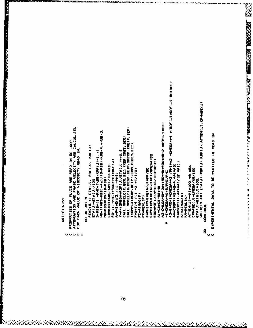
W 8:w

0L W- 4Lm4 !Ii

0; - a . w wiz 3f 0+.w Ur

aw- f: "-

g W, .2

-j W- m% .~ ; ý

Lt.a Oc~m ~ I4I2

WO.-- 4 inT;

U U .U

76

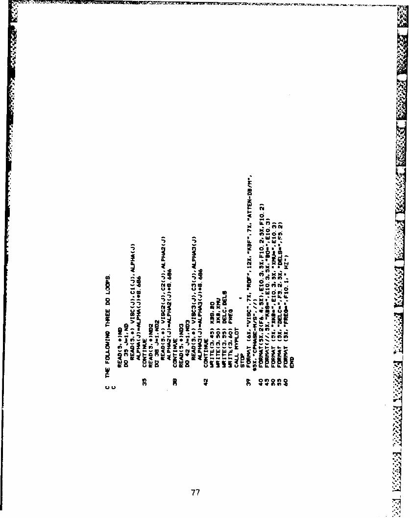
tI

Q x 0 ••[,3 --

V 16- 0 IV...

L I-

S• ~~*. UI•IO .'

- - -a -*oW•.

a .¶ *a

1.3* lot inn.U9 UU WO

77 "

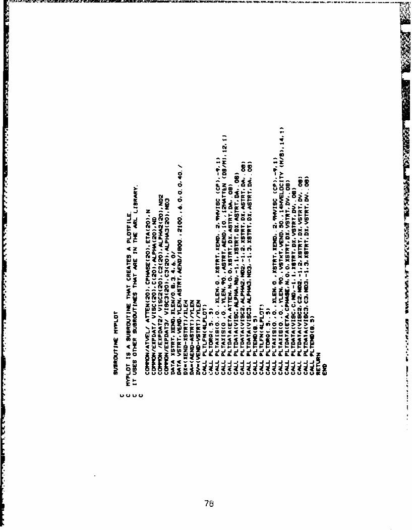
cinSi0000

.8c

2 ! o - I--

A~~ bcIL

4 0 *bco.. m

*i2

00

a;_70

APPENDIX B

EXPERIMENTAL DATA

BEAD TYPE: MS-MH

FREQUENCY: 105.0 kHz VISCOSITY: 0.593 cP

AMPLITUDE - volts TIME - gs SEPARATION - cm

0.3720 65.88 5.650.2690 77.63 7.650.2004 88.98 9.650.1570 100.12 11.650.1300 112.07 13.650.1074 121.38 15.650.0892 133.23 17.650.0777 142.31 19.65

VELOCITY: 1820.0 m/sSTANDARD DEVIATION OF VELOCITY: 23.6 m/s

LINEAR CORRELATION COEFFICIENT: 0.9Q95

ATTENUATION: 2.38 Np/mSTANDARD DEVIATION OF ATTENUATION: 0.47 Np/m

79

79 r

BEAD TYPE: MS-MH

FREQUENCY: 105.0 kHz VISCOSITY: 0.893 cP

AMPLITUDE - volts TIME - SEPARATION - cm

0.1286 62.21 5.650.0907 73.60 7.650.0690 84.04 9.650.0542 94.83 11.650.0440 105.90 13.650.0366 115.97 15.650.0309 126.98 17.650.0266 137.16 19.65

VELOCITY: 1869.7 m/sSTANDARD DEVIATION OF VELOCITY: 9.0 m/sLINEAR CORRELATION COEFFICIENT: 0.9999

ATTENUATION: 2.38 Np/mSTANDARD DEVIATION OF ATTENUATION: 0.12 Np/m

8O4

BEAD TYPE: MS-MH

FREQUENCY: 105.0 kHz VISCOSITY: 1.07 cP

AMPLITUDE - volts TIME - jus SEPARATION - cryi

0.1310 61.69 5.650.0912 72.61 7.650.0696 82.62 9.650.0547 93.72 11.650.0441 104.37 13.650. 0%57 2 1 15.05 15.650.0310 126.53 17.650.0268 136.68 19.65

VELOCITY: 1861.3 m/sSTANDARD DEVIATION OF VELOCITY: 6.8 m/sLINEAR CORRELATION COEFFICIENT: 0.9999

ATTENUATION: 2.46 Np/mSTANDARD DEVIATION OF ATTENUATION: 0.25 Np/m

81

BEAD TYPE: MS-MH

FREQUENCY: 105.0 kHz VISCOS1TY: 1.22 cP

AMPLITUDE - volts TIME - gs SEPARATION - cm

0.1325 61.17 5.650.0928 71.66 7.650.0702 82.34 9.650.0550 92.80 11.650.0448 103.58 13.650.0370 114.31 15.650.0321 124.96 17.650.0270 135.59 19.65

VELOCITY: 1878.9 rn/sSTANDARD DEVIATION OF VELOCITY: 2.6 m/sLINEAR CORRELATION COEFFICIENT: 1.0000

ATTENUATION: 2.42 Np/mrSTANDARD DEVIATION OF ATTENUATION: 0.36 Np/r I:

82

BEAD TYPE: MS-MHFREQUENCY: 105.0 kHz VISCOSITY: 1.33 cP

AMPLITUDE - volts TIME - s SEPARATION - cm

0.1280 60.74 5.660.0916 71.00 7.660.0697 81.30 9.630.0544 92.02 11.650.0445 102.42 13.620.0375 112.98 15.610.0320 123.17 17.610.0274 134.40 19.63

VELOCITY: 1898.6 m/sSTANDARD DEVIATION OF VELOCITY: 5.7 m/sLINEAR CORRELATION COEFFICIENT: 1.0000

ATTENUATION: 2.18 Np/mSTANDARD DEVIATION OF ATTENUATION: 0.22 Np/m

83

BEAD TYPE: MS-MHFREQUENCY: 105.0 kHz VI5COSITY: 1.33 cP

AMPLI'tUt" - volts 11ME1 - pS SEFARATION - cm

0.1310 60.97 5.670.0920 71.20 7.640.0707 81.59 9.620.0546 92.60 11.640.0443 103.14 13.630.0370 113.47 15.620.0316 124.25 17.650.0275 134.22 19.58

VELOCITY: 1893.3 mls

STANDARD DEVIATION OF VELOCITY: 4.2 m/sLINEAR CORRELATION COEFFICIENT: 1.0000

ATTENUATION: 2.35 Np/mrSTANDARD DEVIATION OF ATTENUATION: 0.33 Np/m

84

BEAD TYPE: MS-MH

FREQUENCY: 105.0 kHz VISCOSITY: 0.893 cP

AAMPLITUDE - volts TIME - ps SEPARATION - cm

0.1193 63.61 6.00.0890 73.32 8.00.0654 85.83 10.00.0526 95.53 12.00.0430 106.16 14.00.0352 117.32 16.00.0300 128.65 18.00.0258 139.50 20.0

VELOCITY: 1839.4 m/sSTANDARD DEVIATION OF VELOCITY: 15.2 m/s

LINEAR CORRELATION COEFFICIENT: 0.9996

ATTENUATION: 2.50 Np/mSTANDARD DEVIATION OF ATTENUATION: 0.29 Np/m

85

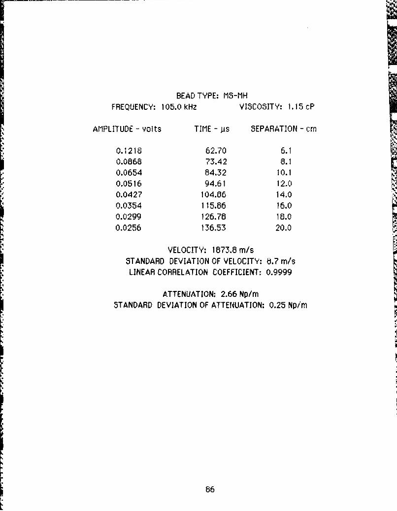
UBEAD TYPE: MS-MH

FREQUENCY: 105.0 kHz VISCOSITY: 1.15 cP

AMPLITUDE - volts TIME - jis SEPARATION - cm

0.1218 62.70 6.10.0868 73.42 8.10.0654 84.32 10.10.0516 94.61 12.00.0427 104.06 14.00.0354 115.66 16.00.0299 126.78 18.00.0256 136.53 20.0

VELOCITY: 1873.8 m/sSTANDARD DEVIATION OF VELOCITY: 8.? m/s

LINEAR CORRELATION COEFFICIENT: 0.9999

ATTENUATION: 2.66 Np/mSTANDARD DEVIATION OF ATTENUATION: 0.25 Np/m

86

1

BEAD TYPE: MS-MHFREQUENCY: 105.0 kHz VISCOSITY: 1.48 cP

AMPLITUDE - volts TIME - js SEPARATION - cm

0.1190 62.02 6.050.0850 72.65 8.090.0646 82.73 10.000.0516 92.36 12.050.0416 102.45 14.02

. 0.0340 112.99 16.030.0280 123.55 18.050.0238 132.91 20.00

VELOCITY: 1966.7 m/sSTANDARD DEVIATION OF VELOCITY: 9.4 m/sLINEAR CORRELATION COEFFICIENT: 0.9999

ATTENUATION: 2.99 Np/mSTANDARD DEVIATION OF ATTENUATION: 0.41 Np/m

87

BEAD TYPE: MS-MHSFREQUENCY: 105.0 kHz VISCOSITY: 1.74 cP

AMPLITUDE - volts TIME - ps SEPARATION - cm

0.1193 61.24 6.06

0.0870 71.06 8.020.0649 81.55 10.020.0514 91.70 12.050.0420 102.19 14.050.0350 1 12.25 16.02

S0.0304 121.78 115.02S0.0256 131.66 20.00

VELOCITY: 1973.3 m/sSTANDARD DEVIATION OF VELOCITY: 8.9 m/s

LINEAR CORRELATION COEFFICIENT: 0.9999

ATTENUATION: 2.41 Np/mSTANDARD DEVIATION OF ATTENUATION: 0.33 Np/m

88

BEAD TYPE: MS-MH

FREQUENCY: 105.0 kHz VISCOSITY: 2.25 cP

AMPLITUDE - volts TIME - jis SEPARATION - cm

0.1180 61.42 6.060.0860 70.69 8.030.0645 80.80 10.060.0515 90.20 12.000.0419 100.52 14.040,0346 110.25 16.030.0296 119,?7 18.000.0258 129.16 20.00

VELOCITY: 2044.1 m/sSTANDARD DEVIATION OF VELOCITY: 7.3 m/sLINEAR CORRELATION COEFFICIENT: 1.0000

ATTENUATION: 2.42 Np/mSTANDARD DEVIATION OF ATTENUATION: 0.19 Np/m

89

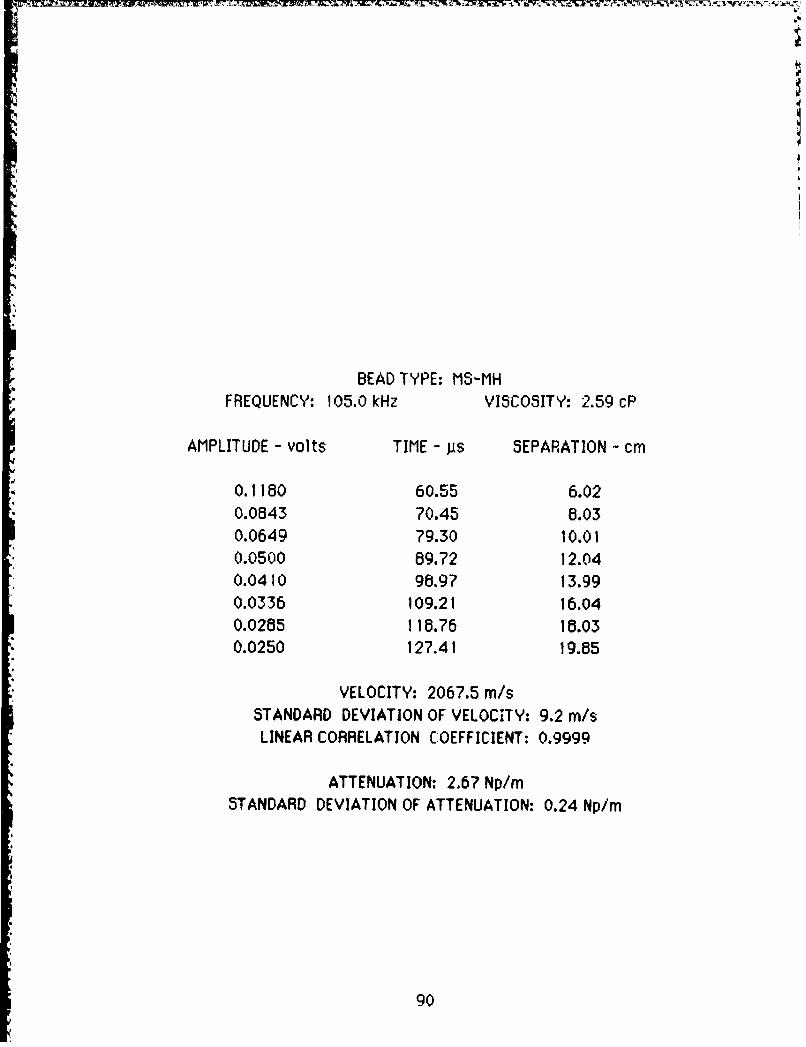
BEAD TYPE: MS-MH

FREQUENCY: 105.0 kHz VISCOSITY: 2.59 cP

AMPLITUDE - volts TIME - gs SEPARATION - cm

0.1180 60.55 6.020.0843 70.45 8.030.0649 79.30 10.010.0500 89.72 12.040.0410 98.97 13.990.0336 109.21 16.040.0285 1 18.76 18.030.0250 127.41 19.85

VELOCITY: 2067.5 m/sSTANDARD DEVIATION OF VELOCITY: 9.2 m/sLINEAR CORRELATION COEFFICIENT: 0.9999

ATTENUATION: 2.6? Np/mSTANDARD DEVIATION OF ATTENUATION: 0.24 Np/m

90

ii

BEAD TYPE: MS-MHFREQUENCY: 105.0 kHz VISCOSITY: 2.81 cP

AMPLITUDE - volts TIME - us SEPARATION - cm

0.1190 60.41 6.04"0.0846 70.00 8.030.0640 79.91 10.050.0505 89.64 12.020.0408 99.09 14.010.0340 108.63 16.000.0282 119.06 18.060.0245 126.97 19.96

VELOCITY: 2074.5 m/sSTANDARD DEVIATION OF VELOCITY: 13.0 m/s

LINEAR CORRELATION COEFFICIENT: 0.9999

ATTENUATION: 2.80 Np/mSTANDARD DEVIATION OF ATTENUATION: 0. 16 Np/m

91

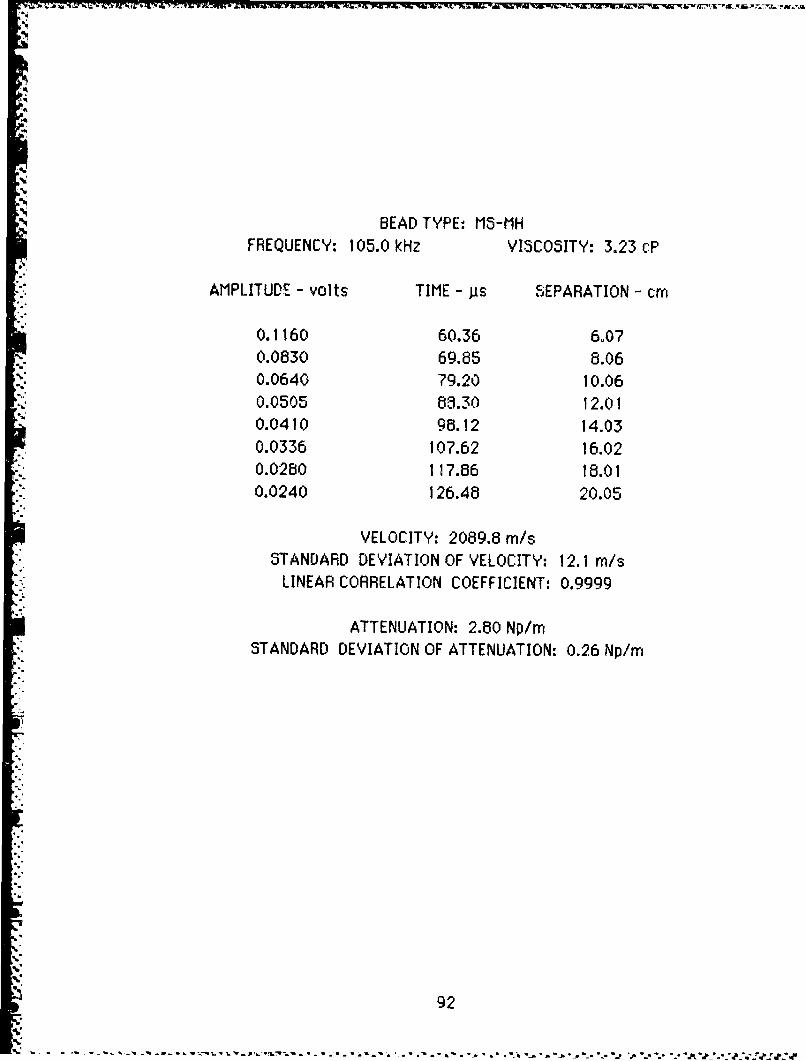
BEAD TYPE: MS-MH

FREQUENCY: 105.0 kHz VISCOSITY: 3.23 cP

AMPLITUDE - volts TIME - us SEPARATION - cm

0.1160 60.36 6.070.0830 69.85 8.06"0.0640 79.20 10.060.0505 63.30 12.010.0410 98.12 14.030.0336 107.62 16.020.0280 117.86 18.010.0240 126.48 20.05

VELOCITY: 2089.8 m/sSTANDARD DEVIATION OF VELOCITY: 12.1 m/s

"* LINEAR CORRELATION COEFFICIENT: 0.9999

ATTENUATION: 2.80 Np/mSTANDARD DEVIATION OF ATTENUATION: 0.26 Np/m

.9

%92

i";

- 92 .% 'L ~ -. n ~ * ~ . ~ t * ~ . , p p

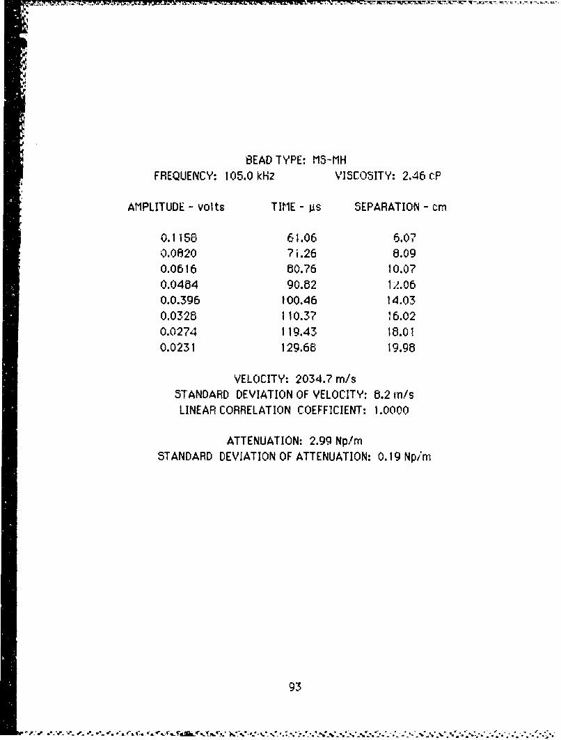
i

4

BEAD TYPE: MS-MH

FREQUENCY: 105.0 kHz VISCOSITY: 2.46 cP

AMPLITUDE - volts TIME - gs SEPARATION - cm

0.1158 61.06 6.070.0820 7 i.26 8.090.0616 80.76 10.070.04a4 90.82 1.060.0.396 100.46 14.030.0328 110.37 16.020.0274 119.43 18.010.0231 129.68 19.98

VELOCITY: 2034.7 m/sSTANDARD DEVIATION OF VELOCITY: 8.2 in/sLINEAR CORRELATION COEFFICIENT: 1.0000

ATTENUATION: 2.99 Np/mSTANDARD DEVIATION OF ATTENUATION: 0.19 Np/m

93

=""e" ' " "" .. • '.-' " .T '• •'•_',.••.•.r¢ ' '•..q•', " w .-. '.••',• . .'_•,•.".. .°," .".".% -. ",.. '.• " . ,. .,A , A ... " .. .. ".. .", " "'"• .. '

BEAD TYPE: MS-MH

FREQUENCY: 105.0 kHz VISCOSITY: 2.09 cP

AMPLITUDE - volts TIME - jis SEPARATION - cm

0.1210 61.73 6.010.0870 71.60 8.020.0660 62.32 10.060.0526 91.83 12.020.0429 101.86 14.000.0355 112.19 16.020.0302 122.23 18.020.0262 132.08 19.99

VELOCITY: 1986.6 m/sSTANDARD DEVIATION OF VELOCITY. 3.6 M/s

LINEAR CORRELATION COEFFICIENT: 1.0000

"ATTENUATION: 2.39 Np/miSTANDARD DEVIATION OF ATTENUATION: 0. 19 Np/m

94

* .

REFERENCES

Bedford, A., G. Ellis, K. P. Eiliot, S. K. Mitchell, D. J. Shirley,"Acoustical Properties of Sediments," Applied ResearchLaboratories Technical Report No. 62-47 (ARL-TR-82-47), AppliedResearch Laboratories, The University of Texas at Austin (1982).

Bedford, A., R. D. Costley, and M. Stern, "On the Drag and Virtual MassCoefficients in Biot's Equations," J. Acoust. Soc. Am. 76, 1804-1809(1984).

Bell, David W., "Shear Wave Propagation in Unconsolidated FluidSaturated Porous Media," Applied Research Laboratories TechnicalReport No. 79-31 (ARL-.TR-79-31), Applied Research Laboratories,The University of Texas at Austin (1979).

Bevington, Philip R., "Data Reduction and Error Analysis for thePhysical Sciences" (McGraw-Hill, Book Co., Inc., New York, 1969).

Biot, M A., "Theory of Propagation of Elastic Waves in a Fluid-SaturatedPorous Solid. I. Low Frequency Range," J. Acoust. Soc. Am. 28,16•-178 (1956a).

Biot, M. A., "Theory of Propagation of Elastic Waves in a Fluid-SaturatedPorous Solid. II. Higher Frequency Range," J. Acoust. Soc. Am 28,179-191 (1956b).

Biot., M. A., " Generalized Theory of Acoustic Propagation in PorousDissipative Media," J. Acoust. Soc. Am. 34, 1254- 1264 (1956c).

Biackstock, David T., Notes from "Acoustics I and II," courses givenin the Departments of Mechanical Engineering and ElectricalEngineering at The University of Texas at Austin.

95

Greenspan, Martin, "Acoustic Properties of Liquids.," in American

Institute of Physics Handbook. 3rd ed., Dwight E. Gray,ed. (McGraw-Hill Book Co., Inc., New York, 1963), pp. 3-79.

Hovem, J. M., and G. D. Ingram, "Viscouls Attenuation of Sound inSaturated Send," J. Acoust. Soc. Am. 6_.6, 1807- 1811I (1979).

Kinsler, L. E., A. R. Frey, A. B. Coppens, and J. V. Sanders, Fundamentals.. of Acoustics, 3rd ed. (John Wiley & Sons, Inc., New York, 1982),• . p. 46 1.

-- %,Sheely, Madison L., Industrial and Engineering Chemistry 24,1060-64 (1932).

Shirley, Donald J., and David W.BelI, "Acoustics of in Situ andLaboratory Sediments," Applied Research Laboratories TechnicalReport No. 78-36 (ARL-TR-78-36), Applied Research Labor~atories.,The University of Texas at Austin (1978).

Stoll, R. D., "Acoustic Waves in Saturated Sediments," in Physics ofSound it) Marine Sediments, L. D. Hampton , ed. (Plenum Press.,New York, 1974), pp. 19-39.

Stoll, R. D., "Acoustic Waves in Ocean Sediments," Geophysics 4__2,715-725 (1977).

96

ACKNOWLEDGMENTS

The author was fortunate to receive contributions and support

from several persons. Dr. A. Bedford supervised this research and was an

appreciated source of encouragement and patience. Dr. Paul Vidmar made

many contributions and suggestions.

Dr. Ilene Busch-Vishniac answered my many questions,

particularly those involving the design of the transducers and error

* analysis. The transducer design was primarily the result of two

conversations with Dr. Elmer Hixson. Mr. Ken Kirksey made several

contributions in the development of the transducers, particularly in their

construction. Dr. David Blackstock was very encouraging and referred me

to several helpful sources. I was also fortunate to visit Mr. James

Matthews' lab at NORDA and to witness some of the progress he has made

in experimental sediment acoustics. Dr. George B. Thurston advised me on

the viscosity measurements. I am indebted to Mr. Donald J. Shirley and

Mr. Kenneth P. Elliot, who both preceded me in the sediments lab at

ARL:UT. The experiment was the brain child of Mr. Shirley.

Ms. Jo Lindberg and Mr. James TenCate made several

contributions concerning instrumentation.

This research was supported by the Office of Naval Research,

Code 425GG and Code 400, and was submitted to the Graduate School of

The University of Texas at Austin in partial fulfillment of the

requirements for the degree of Master of Science in Engineering.

97

May 1985

DISTRIBUTION LIST FORARL-TR-85-14

UNDER CONTRACT N00014-80-C-0490

Copy No.

Office of Naval Research495 Summer StreetBoston, MA 02210

1 Attn: R. L. Sternberg

Commanding OfficerNaval Ocean Research and Development ActivityNSTL Station, MS 39529

2 Attn: E. D. Chaika (Code 530)3 D. B. King (Code 321)4 R. Wagstaff (Code 245)5 K. Gilbert (Code 221)6 A. Wenzel7 G. Morris (Code 425GG)8 J. Matthews (Code 362)

Chief of Naval ResearchDepartment of the NavyArlington, VA 22217

9 Attn: M. McKisic (Code 425-OA)10 R. Obrochta (Code 425-AR)11 F. E. Saalfield (Code 400)

DirectorNaval Research LaboratoryDepartment of the NavyWashington, DC 20375

12 Attn: 0. Diachok (Code 5128)13 R. Dicus (Code 5128)14 R. Gragg

Lawrence Livermore National LaboratoryP. 0. Box 808, L-200Livermore, CA 94550

15 Attn: J. G. Berryman

Planning Systems, Inc.7900 Westpark DriveSuite 600McLean, VA 22102

16 Attn: B. Brunson

99

Distribution List for ARL-TR-85.-14 under Contract N00014-80-C-0490(cont'd)

Copy No.Lamont-Daherty Geological Observatory

Columbia UriversityPalisades, NY 10964

17 Attn: R. D. Stoll

18 A. Mark Bedford, ARL:IJT

19 H. Boehme, ARL:UT

^.0 Ilene J. Busch-Vishniac, ARL:UT

21 Karl C. Focke, ARL:UT

22 Thomas A. Griffy, ARL:UT

23 John M. Huckabay, ARL:UT

24 Robert A. Koch, ARL:UT

25 Stephen K. Mitchell, ARL:UT

26 T. G. Muir, ARL:UT

27 David W. Oakley, ARL:UT

28 Clark S. Penrod, ARL-UT

29 3orris Stern. ARL:UT

2) James A. TenCate, ARL:UI

31 Paul J. Vidmar, ARL:UT

32 Gary R. Wilson, ARL:UT

33 H. Yew, ARL:UT

34 Library, ARL:UT

100