Technetium and Iodine Getters to Improve Cast Stone Performance

PNNL-23282 Rev 1

Prepared for the U.S. Department of Energy under Contract DE-AC05-76RL01830

Technetium and Iodine Getters to Improve Cast Stone Performance NP Qafoku RJ Serne JJ Neeway JH Westsik, Jr AR Lawter MM Valenta Snyder TG Levitskaia February 2015

PNNL-23282 Rev 1

Technetium and Iodine Getters to Improve Cast Stone Performance NP Qafoku RJ Serne

JJ Neeway JH Westsik, Jr

AR Lawter MM Valenta Snyder TG Levitskaia

February 2015 Prepared for the U.S. Department of Energy under Contract DE-AC05-76RL01830 Pacific Northwest National Laboratory Richland, Washington 99352

iii

Executive Summary

Washington River Protection Solutions is collecting relevant available data on waste forms to provide the additional capacity for treating all of the low-activity waste (LAW) from the Hanford waste tanks. Four alternatives have been considered for supplemental immobilization of the LAW, but two, baseline vitrification and a low-temperature immobilization process based on a cementitious grout called Cast Stone, are the current front runners. In addition, Cast Stone has been selected as the preferred waste form for solidification of aqueous secondary liquid effluents from the Hanford Tank Waste Treatment and Immobilization Plant process condensates and LAW melter off-gas caustic scrubber effluents. Cast Stone is also being evaluated as a supplemental immobilization technology to provide the necessary LAW treatment capacity to complete the tank waste cleanup mission in a timely and cost-effective manner.

The Tank Closure and Waste Management Environmental Impact Statement for the Hanford Site, Richland, Washington (TC&WM EIS) identifies technetium-99 (99Tc) and iodine-129 (129I) as radioactive tank waste components contributing the most to the environmental impacts associated with the cleanup of the Hanford Site. A diffusion-limited release model was used in both the TC&WM EIS and an earlier supplemental waste-form risk assessment to estimate the release of different contaminants from the WTP process waste forms. Effective diffusivities (the metric used to quantify release from the Cast Stone waste form) for these two key contaminants used in the two analyses ranged from 3 × 10-10 to 5 × 10-9 cm2/s for Tc and 1.0 × 10-10 to 2.5 × 10-9 cm2/s for I. In both of these predictive modeling exercises, groundwater at the 100-m down-gradient well exceeded the allowable maximum permissible concentrations for both contaminants.

Recent relatively short-term (63 day) leach tests conducted on both LAW and secondary waste Cast Stone monoliths indicated that Tc diffusivities were in the range of 5 × 10-12 to 3 × 10-10 cm2/s, and iodide diffusivities were in the range of <4 × 10-10 to 2 × 10-8 cm2/s. There is, therefore, a need and an opportunity to improve the retention of Tc and I in the Cast Stone waste forms. One method of improving the performance of the Cast Stone waste forms is to add “getters” that selectively sequester contaminants of concern. Getters can be used in two modes. In the first mode, the getter is added to the aqueous wastes where it scavenges the specific contaminant(s) of interest from the liquid waste. The loaded getter is then removed from the liquid and is immobilized in a separate waste form. In the second mode, the getter is added to either the liquid waste or the Cast Stone dry blend reagents and become part of the final waste form.

To determine the effectiveness of the various getter materials prior to their solidification in Cast Stone, a series of batch sorption experiments was performed at Pacific Northwest National Laboratory. To quantify the effectiveness of the removal of Tc(VII) and I(I) from solution by getters, the distribution coefficient, Kd (mL/g), was calculated. Testing involved placing getter material in contact with spiked waste solutions at a 1:100 solid-to-solution ratio for periods up to 45 days with periodic solution sampling. One Tc getter was also tested at a 1:10 solid-to-solution ratio.

Two different solution media, 18.2 MΩ deionized water (DI H2O) and a 7.8 M Na LAW simulant, were used in the batch sorption tests. Each test was conducted at room temperature in an anoxic chamber containing N2 with a small amount of H2 (0.7%) to maintain anoxic conditions. Each getter-solution combination was run in duplicate. Three Tc- and I-doping concentrations were used separately in aliquots of both the 18.2 MΩ DI H2O and a 7.8 M Na LAW waste simulant. The 1× concentration was developed

iv

based on Hanford Tank Waste Operations Simulator (HTWOS) model runs to support the River Protection Project System Plan Revision 6. The other two concentrations were 5× and 10× of the HTWOS values.

The Tc and I tests were run separately (i.e., the solutions did not contain both solutes). Sampling of the solid-solution mixtures occurred nominally after 0.2, 1, 3, 6, 9, 12, 15 days and ~35 to 45 days. Seven getter materials were tested for Tc and five materials were tested for I. The seven Tc getters were blast furnace slag 1 (BFS1) (northwest source), BFS2 (southeast source), Sn(II)-treated apatite, Sn(II) chloride, nano tin phosphate, KMS (a potassium-metal-sulfide), and tin hydroxapatite. The five iodine getters were layered bismuth hydroxide (LBH), argentite mineral, synthetic argentite, silver-treated carbon, and silver-treated zeolite.

The Tc Kd values measured from experiments conducted using the 7.8 M Na LAW simulant (the simulant selected to represent LAW) for the first 15 days for four Tc getters (BFS1, BFS2, Sn(II)-treated apatite, and Sn(II) chloride) show no, to a very small, capacity to remove Tc from the LAW simulant. For the Tc-getter experiments in the 7.8 M LAW simulant, the majority of the effluent samples show very small drops in Tc concentrations for the 35-day compared to the 15-day samplings. However, the Tc concentration in the simulant blanks also dropped slightly during this period, so the effect of the getter contacting LAW simulant at 35 days compared to 15 days is minimal; except that the BFS1 1:10 test shows a slow but steady decrease in Tc concentration in the LAW simulant supernatant from the beginning to the 35 day contact at which point about 20% of the original Tc has been removed from solution. Lastly, the KMS getter gives the highest Kd value for Tc at 35 days where Kd values have increased to 104 mL/g.

When considering the different I getters reacting with the 7.8 M LAW simulant, two getters are much more effective than the others: Ag zeolite and Syn Arg. The other getters have calculated iodide distribution coefficients that show very limited effectiveness in the caustic conditions created by the LAW simulant.

These are preliminary results that will need more detailed analyses including both pre- and post-batch sorption getter solid-phase characterization using state-of-the-art instrumentation such as synchrotron X-ray absorption spectroscopy, which can delineate the oxidation state of the Tc and likely iodine species as well as some of the getters key major components, sulfur and iron in the BFS, and tin and sulfur in the tin-bearing and sulfur-bearing getters.

This report also describes future experimental studies to be performed to better elucidate the mechanisms controlling the Tc and I sequestration processes in the various getters and leach tests of getter-bearing Cast Stone monoliths.

v

Acknowledgments

This work was completed as part of the Supplemental Immobilization of Hanford Low-Activity Waste project. Support for this project came from the U.S. Department of Energy’s Office of Environment Management. NP Qafoku, RJ Serne, JJ Neeway, and JH Westsik, Jr contributed equally to this study and the report.

The authors wish to acknowledge Brian Riley for providing one of the technetium getters, and Dave Swanberg (Washington River Protection Solutions, Supplemental Treatment Waste Form Development Project) for programmatic guidance, direction, and support and for synthetizing and providing the tin apatite material used in this study.

The authors wish to thank Dr. Kirk Cantrell for his technical peer review and Susan Ennor and Kathy Neiderhiser for editorial review and document production.

vii

Acronyms and Abbreviations

ASTM American Society for Testing and Materials

BET Brunauer–Emmett–Teller

BFS blast furnace slag

cm2/s square centimeter(s) per second

Cu copper

DDI deionized distilled

DIW deionized water

DOE U.S. Department of Energy

DOE/ORP Department of Energy – Office of River Protection

EPA U.S. Environmental Protection Agency

EQL Estimated Quantitation Limit

EXAFS extended X-ray absorption fine structure spectroscopy

GWPS groundwater protection standard

HMS heavy metals sludge

HTWOS Hanford Tank Waste Operations Simulator

I iodine

ICP-MS inductively coupled plasma mass spectroscopy

IDF Integrated Disposal Facility

Kd distribution coefficient

LAW (Hanford) low-activity waste

LBH layered bismuth hydroxide

LI leach index

m meter(s)

m2/g square meter per gram

MCL maximum contaminant level

MPC maximum permissible concentration

Na sodium

NW Northwest

Ni nickel

PNNL Pacific Northwest National Laboratory

ppm parts per millions

PTFE polytetrafluoroethylene

RCRA Resource Conservation and Recovery Act of 1976

s second(s)

SE Southeast

viii

Si silicon

SRNL Savannah River National Laboratory

SRS Savannah River Site

SST single-shell tank

TEM transmission electron microscopy

Tc technetium

TC&WM EIS Tank Closure and Waste Management Environmental Impact Statement

µXRF X-ray fluorescence

XAS X-ray absorption spectroscopy

XANES X-ray absorption near-edge spectroscopy

XPS X-ray photoelectron spectroscopy

ix

Contents

Executive Summary .............................................................................................................................. iii

Acknowledgments ................................................................................................................................. v

Acronyms and Abbreviations ............................................................................................................... vii

1.0 Introduction and Background ....................................................................................................... 1.1

1.1 Summary of the Literature Review on Tc and I Getters ...................................................... 1.2

1.2 Objectives ............................................................................................................................. 1.3

1.3 Report Contents and Organization ....................................................................................... 1.4

2.0 Technical Scope and Approach .................................................................................................... 2.1

2.1. Batch Tests ........................................................................................................................... 2.2

2.2. LAW Simulant Preparation .................................................................................................. 2.1

2.3. Getters Used in this Study .................................................................................................... 2.4

2.4. X-ray Diffraction Analyses .................................................................................................. 2.4

2.5. Specific Surface Area ........................................................................................................... 2.5

2.6. Moisture Content and Liquid Phase Analyses ..................................................................... 2.7

3.0 Results and Discussion ................................................................................................................. 3.1

3.1 Moisture Content and Surface Area ..................................................................................... 3.1

3.2 X-ray Diffraction Analyses .................................................................................................. 3.1

3.3 Technetium Getter Distribution Coefficients ....................................................................... 3.3

3.4 Iodine Getters Distribution Coefficients .............................................................................. 3.8

3.5 Behavior of I and Tc at Periods Longer than 15 Days ......................................................... 3.12

3.6 Normalization of Kd Values with the Surface Area ............................................................. 3.12

3.7 Behavior of Other Elements Present in the Simulant ........................................................... 3.13

4.0 Conclusions .................................................................................................................................. 4.1

5.0 Future Studies ............................................................................................................................... 5.1

6.0 References .................................................................................................................................... 6.1

Appendix A – Interactions Between Getters and Cast Stone ................................................................ A.1

Appendix B – X-ray Diffraction Spectra for the Getters Used in this Study ........................................ B.1

Appendix C – Effluent Concentrations, pH Values, and Calculated Kd Values ................................... C.1

x

Figures

3.1. Log Kd values for the four Tc getters tested with an initial [Tc] ≈ 5 ppm in DDI water and 7.8 M Na LAW simulant ........................................................................................................ 3.5

3.2. Log Kd values for the four Tc getters tested with an initial [Tc] ≈ 27 ppm in DDI water and 7.8 M Na LAW simulant ........................................................................................................ 3.6

3.3. Log Kd values for the eight Tc getters tested with an initial [Tc] ≈ 53 ppm in DDI water and 7.8 M Na LAW simulant ........................................................................................................ 3.7

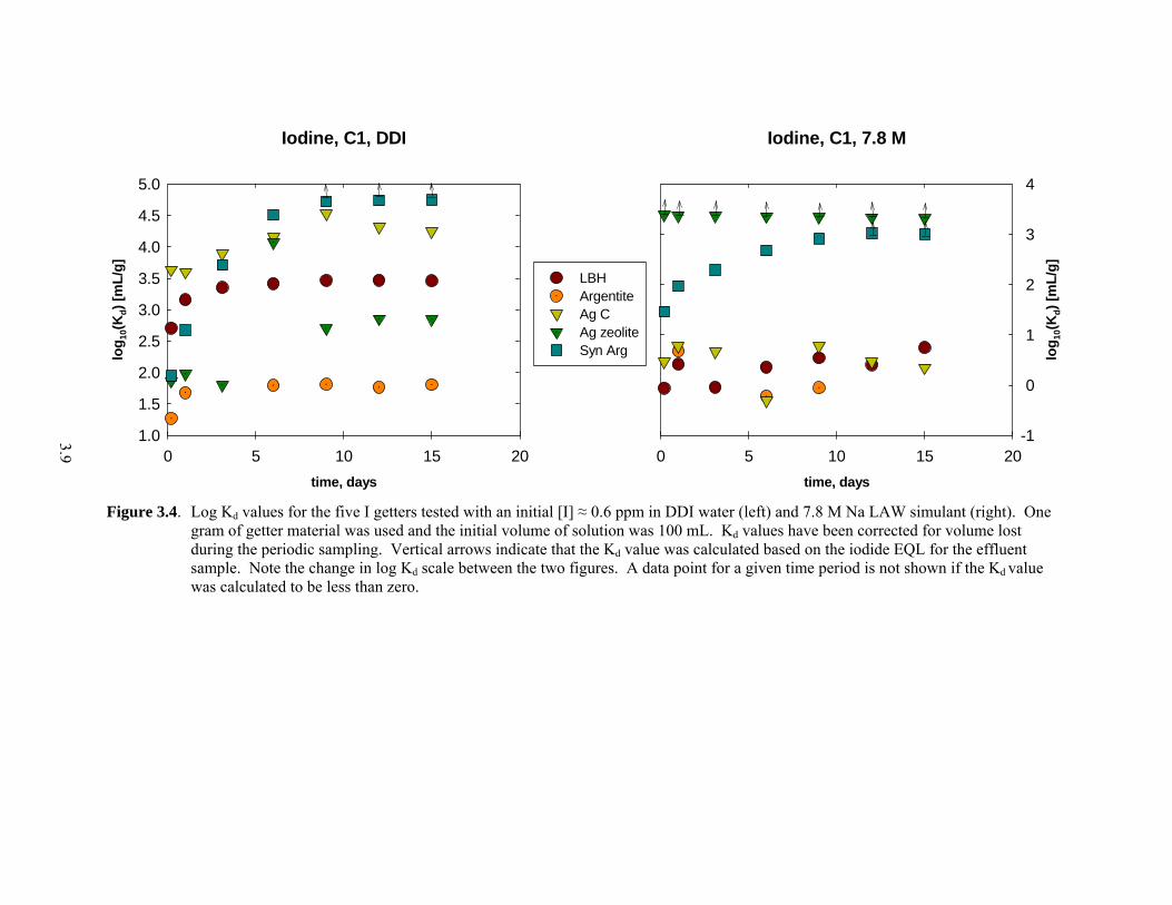
3.4. Log Kd values for the five I getters tested with an initial [I] ≈ 0.6 ppm in DDI water and 7.8 M Na LAW simulant .............................................................................................................. 3.9

3.5. Log Kd values for the five I getters tested with an initial [I] ≈ 3 ppm in DDI water and 7.8 M Na LAW simulant .............................................................................................................. 3.10

3.6. Log Kd values for the five I getters tested with an initial [I] ≈ 6 ppm in DDI water and 7.8 M Na LAW simulant .............................................................................................................. 3.11

Tables

2.1. Screening test matrix for various Tc and I getters ........................................................................ 2.3

2.2. The solution concentration for various dosages of Tc and I at the beginning of the experiment .................................................................................................................................... 2.4

2.3. Simulant for LAW to be used in getters tests ............................................................................... 2.1

2.4. List and origin of the getter materials used in the experiment ...................................................... 2.6

3.1. Moisture content and surface area of the 12 getters used in testing .............................................. 3.1

3.2. Concentration of Cr in the LAW simulant effluents from Tc batch tests at 0.2 and 15 days for various getters ................................................................................................................. 3.14

3.3. Concentration of Cr in the LAW simulant effluents from Tc batch tests at 0.2 and 15 days for various getters ................................................................................................................. 3.14

3.4. Concentration of Cr, Cd, and Pb in LAW Simulant at 0.2 and 15 days for the various getters used in the iodine tests ...................................................................................................... 3.15

1.1

1.0 Introduction and Background

Washington River Protection Solutions is collating available data and, for some waste forms, generating new data on the performance of different waste forms suitable for stabilizing Hanford low-activity waste (LAW). Four alternatives have been considered for supplemental immobilization of the LAW but two, increasing the capacity of the baseline LAW vitrification facility and a low-temperature immobilization process based on a cementitious grout called Cast Stone, are the current front runners. Cast Stone has been selected as the preferred waste form for solidification of the Hanford Tank Waste Treatment and Immobilization Plant secondary liquid effluents from process condensates and LAW melter off-gas caustic scrubber effluents. The Cast Stone baseline dry blend mix currently used is 8 wt% Portland cement Type I/II, 45% Class F fly ash, and 47% Grade 100 or 120 blast furnace slag. Based on preliminary studies of secondary waste simulants (Sundaram et al. 2011; Mattigod et al. 2011a), other data reviewed by Serne and Westsik (2011), and the general similarity of liquid secondary wastes to LAW (both are high-sodium, nitrate-dominated caustic brines), Cast Stone may also be a worthy candidate for immobilization of liquid LAWs. Therefore, Cast Stone is also being evaluated as a supplemental immobilization technology to provide the necessary LAW treatment capacity to complete the tank waste cleanup mission in a timely and cost-effective manner.

Performance assessment tests are used to evaluate the potential environmental impact from disposal of LAW forms. At the Hanford Site the current plan is to dispose the immobilized low-activity waste (ILAW) and the solidified secondary wastes in the Integrated Disposal Facility (IDF) located in 200-E Area. Past (Mann et al. 2001) performance assessments and risk assessments (Mann et al. 2003 and DOE 2012) show that releases from LAW disposal might not meet environmental protection standards over long periods of time. All three of these assessments use diffusion-controlled release models for contaminants from grouts. Table 1.1 shows the effective diffusion coefficients used for 99Tc and 129I in these assessments. These effective diffusion coefficients were taken from grout leaching literature available at the time and were not specific for the current formulation of Cast Stone. The values were chosen by experienced waste form release scientists to represent “reasonable” values for the anticipated IDF subsurface conditions.

Table 1.1. Comparison of Effective Diffusion Coefficients (cm2/s) Used in Mann et al. (2001, 2003) and DOE(2012) for grout and/or Cast Stone

Constituent Mann et al. (2001, 2003)

DOE (2012) Ratio Mann/DOE

Tc-99 3.2 × 10-10 5.2 x 10-9 0.062 I-129 2.5 × 10-9 1.0 x 10-10 25

The Mann et al. (2003) preliminary risk assessment for supplemental waste forms suggests that the effective diffusion coefficients for 99Tc and 129I should be somewhat lower than 3.2 × 10-10 and significantly lower than 2.5 × 10-9 cm2/s, respectively, to meet groundwater protection standards likely to be used for the IDF facility. This statement is valid as long as other assumptions in Mann et al. (2003) are retained in future IDF performance assessment projections. We do note that the 99Tc and 129I inventories in Cast Stone used by Mann et al. (2003) include only 25% of the total LAW inventory and current projections for the supplemental waste form may require up to 70% of the LAW inventory to be solidified in the supplemental waste form.

1.2

Over the past three years many Cast Stone leach studies have been performed by waste form experts at both PNNL and SRNL. At PNNL at least four LAW simulants and four secondary waste simulants were solidified into the current baseline recipe for Cast Stone, which as mentioned above uses a dry blend mixture of blast furnace slag (47 wt%), fly ash (45 wt%), and cement (8 wt%). A range of simulant concentrations from 2M Na to 7.8 M Na have been solidified in thie Cast Stone dry blend at a range of water to dry blend mix ratios. The use of blast furnace slag is a key to immobilizing 99Tc through reduction processes controlled by ferrous iron and reduced sulfur species within the blast furnace slag (see more discussion in Serne and Westsik (2011) and Westsik et al. (2014). Monoliths of the final cured Cast Stone waste forms were then leached using up to three standard leaching protocols (EPA 1315, ASTM C1308, and ANSI 16.1)1 for time periods of 63 to over 91 days. The results of these leach tests conducted on both LAW (Westsik et al. 2013) and secondary waste (Mattigod et al. 2011a) Cast Stone monoliths indicated that technetium (99Tc) diffusivities were in the range of 5 × 10-12 to 3 × 10-10 cm2/s, and iodide (stable iodine [127I] was used) diffusivities were in the range of <4 × 10-10 to 2 × 10-8 cm2/s. Given the results of Mann et al. (2003), it appears that the recently measured range in effective diffusion coefficients for 99Tc are within the range that might show acceptable groundwater protection. However, there is concern (see for example (Brown et al. 2013 and Serne and Westsik 2011) that the 99Tc leach performance exhibited in these short term laboratory tests may not account for longer term re-oxidation of Tc in the Cast Stone as the reductants within the blast furnace slag component are depleted by contact with oxygen in vadose zone air and oxygen dissolved in the vadose zone porewater. The recently measured range of effective diffusion coefficients for stable iodide (representative of 129I) is much larger than values that Mann et al. (2003) suggest will be necessary to protect groundwater below the IDF facility.

Therefore, the retention of 99Tc and iodine (129I) in the Cast Stone waste forms needs to be improved. One method of improving the performance of the Cast Stone waste forms is to add “getters” (absorbers) that selectively sequester contaminants of concern. Getters can be used in two modes. In the first mode, the getter is added to the aqueous wastes where it scavenges the specific contaminant(s) of interest from the liquid waste. The loaded getter is then removed from the liquid and is immobilized in a separate waste form. In the second mode, the getter is added to either the liquid waste or the Cast Stone dry blend reagents and becomes part of the final waste form. Currently, only a limited number of studies have thoroughly investigated interactions between getters and Cast Stone waste forms (see Appendix A in this report), and additional experimental work is needed in this area.

1.1 Summary of the Literature Review on Tc and I Getters

A detailed literature review and the corresponding references are included in Appendix A of this report. The literature review identified the following getters as having promising properties for Tc removal and sequestration: nanoporous tin (Sn) phosphates, Sn(II)-treated apatite, and ground blast 1 EPA—U.S. Environmental Protection Agency. 2009c. Mass Transfer Rates of Constituents in Monolith or Compacted Granular Materials Using a Semi-Dynamic Tank Leaching Test. Draft Method 1315, Washington D.C. ASTM— American Society for Testing and Materials. 2008b. Standard Test Method for Accelerated Leach Test for Diffusive Releases from Solidified Waste and a Computer Program to Model Diffusive, Fractional Leaching from Cylindrical Waste Forms. ASTM C 1308, West Conshohocken, Pennsylvania. ANSI—American National Standards Institute. 2003. Measurement of the Leachability of Solidified Low Level Radioactive Waste by a Short-Term Test Procedure. American Nuclear Society, La Grange Park, Illinois.

1.3

furnace slag (BFS). These getters have high affinity for Tc. For example, experimental work conducted with the BFS, demonstrated that BFS possessed relatively high reduction capacities for Tc(VII) that ranged from 0.82 to 4.79 meq/g (Pierce et al. 2010; Mattigod et al. 2011b and the references therein). Distribution coefficient (Kd) values of greater than 90,000 mL/g for Tc sorbed by the nano tin phosphate were found in experiments conducted with a dilute bicarbonate solution (0.002 M NaHCO3 at pH = 8) (Wellman et al. 2006). Even greater Kd values (approximately 3 million mL/g) were reported in a study of Tc sorption to Sn(II)-treated apatite when the Tc aqueous concentration varied between 9.11 × 10-6–9.11 × 10-5 M (Moore 2003, cited by Mattigod et al. 2011b). Considering that the Kd values for pertechnetate (TcO4

-) sorption to common Fe (hydr)oxides found in soils and sediments vary between 0–190 mL/g under oxic or anoxic conditions, the Kd values for these getters are enormously high and very promising.

Layered bismuth hydroxides (LHBs), argentite (Ag2S), silver-impregnated carbon, and silver zeolites are identified in the literature as getters with high affinity for I (Pierce et al. 2010). For example, the Kd values for iodide (I-) and iodate (IO3

-) varied between 631–25,119 and 50–39,811 mg/L, respectively, in experiments conducted with layered Bi hydroxide (Krumhansl et al. 2006, cited by Pierce et al. 2010). In addition, iodide Kd values of up to 80,000 mL/g were reported in experiments conducted with argentite and surface water with pH = 5.98 (Kaplan et al. 2000, cited by Pierce et al. 2010), and I Kd values of 30,000 mL/g were reported in other experiments conducted with argentite and a glass leachate solution with varying pH (2.66 to 8.33) (Mattigod 2003). Finally, I Kd values of 1,000 to 5,000 mL/g were reported in experiments conducted with Ag carbon and surface water with pH = 7.56 (Kaplan et al. 2000, cited by Pierce et al. 2010).

However, the sorption properties of the Tc and I getters vary considerably under different experimental conditions. For example, Mattigod et al. (2011b) reported Kd values between 475,000 and 3,202,100 mL/g for Tc sorption on Sn(II)-treated apatite when groundwater with pH varying from 6 to 10 was used, but Tc Kd values were considerably smaller and varied within a narrower range (between 5,150 and 6,510 mL/g) when a concentrated solution of NaNO3, NaNO2, and NaOH–NaAlO2 at pH = 13 was used as the background contacting solution in experiments conducted with the same material. This concentrated NaNO3, NaNO2, and NaOH–NaAlO2 solution at pH = 13 is more similar to the liquid LAWs that require solidification.

The long-term performance of the getters as part of monolithic waste forms, which is currently unknown, must be evaluated (Pierce et al. 2010). For example, BFS included in the Cast Stone dry blend mixture has been shown to be effective at reducing Tc(VII) to the less mobile Tc(IV) oxidation state, resulting in improved retention of Tc in the Cast Stone as long as reducing conditions prevail. However, past experimental work has also demonstrated that the BFS getter-based waste forms may release Tc as a result of oxidation of Tc2S7 in the presence of O2. One key tenet is that getters should not adversely affect the waste-form performance. Experimental work is required to determine the effectiveness of the various getter materials prior to their solidification in Cast Stone.

1.2 Objectives

The overall objectives of the testing program were to 1) determine an acceptable formulation for the LAW Cast Stone waste form with getters, 2) demonstrate the robustness of the formulation in terms of Tc and I release diffusivities, and 3) provide Cast Stone contaminant release data for risk assessment

1.4

evaluations. The specific objective for this part of the study was to investigate Tc and I getters’ performance under conditions relevant to those of the waste streams. A series of batch experiments was conducted to address this objective. The experiments were conducted under strict anaerobic conditions inside chambers with controlled atmosphere (in absence of air) to allow for a better estimation of the getters’ reduction capacity in the absence of competing electron acceptors, such as O2. Future planned studies will investigate the potential benefits of adding getters to improve the retention of Tc and I in the Cast Stone waste form and the compatibility of getters with the Cast Stone, and will determine improvements in controlling the release of Tc and I for getters incorporated into Cast Stone. Specifically, the robustness of getter/Cast Stone formulations will be investigated in terms of determining the Tc and I release diffusivities.

1.3 Report Contents and Organization

The ensuing sections of this report describe the technical scope and approach of the testing program, present and discuss the results and conclusions, and identify future study needs. The appendixes contain information about the interactions between getters and Cast Stone (Appendix A); X-ray diffraction spectra for the getters used in this study (Appendix B); and effluent concentrations, calculated Kd values, and pH values (Appendix C).

2.1

2.0 Technical Scope and Approach

The testing program included the conduct of batch tests, preparation of the LAW simulant used to represent the tank LAWs, testing of getter materials and their analysis using X-ray diffraction; as well as the analysis of getter surface area, porosity, pore size, and its gravimetric water content, as described in the following sections.

2.1 Quality Assurance

All research and development (R&D) work at PNNL is performed in accordance with PNNL's Laboratory-level Quality Management Program, which is based on a graded application of NQA-1-2000, Quality Assurance Requirements for Nuclear Facility Applications, to R&D activities. To ensure that all client quality assurance (QA) expectations were addressed, the QA controls of the WRPS Waste Form Testing Program (WWFTP) QA program were also implemented for this work. The WWFTP QA program consists of the WRPS Waste Form Testing Program Quality Assurance Plan (QA-WWFTP-001) and associated QA-NSLW-numbered procedures that provide detailed instructions for implementing NQA-1 QA requirements for R&D work.

The work described in this report was assigned the technology level “Basic Research” and was planned, performed, documented, and reported in accordance with Procedure QA-EMSP-1101, Scientific Investigation for Basic Research. All staff members contributing to the work received proper technical and quality assurance training prior to performing quality-affecting work.

The work performed in this report addresses the tasks described in WRPS statement of work (SOW) 36437-134, “Supplemental Immobilization of Hanford Low Activity Waste.”

2.1. LAW Simulant Preparation

One LAW simulant was selected to represent the LAWs in tanks and was used in the batch experiments described above. The list of chemicals, added to the solution in descending order, is given in Table 2.1. This is the simulant used in the LAW Cast Stone screening tests that was named 7.8 M Na Ave (see Westsik et al. [2013] for more details). The simulant was developed based on HTWOS model runs to support the River Protection Project System Plan Revision 6 (Certa et al. 2011). As one of the outputs, the HWTOS model provides the feed vector to a supplemental immobilization facility over the course of the tank waste treatment mission. The resulting values for various anions and cations are also given in Table 2.. It should be noted that undissolved solids remained when the solution preparation was complete. Based on notes taken during the preparation, the solid is more likely a Na-phosphate and/or Na-fluoride and small amounts of Ni salt (Ni-nitrate was added but did not completely dissolve).

Table 2.1. Simulant for LAW to be used in getters tests.

Compound Amount,

g/L Waste

Constituent HTWOS Overall Average, mol/L

Theoretical Concentration,

mmol/L(a) Al(NO3)3•9H2O 179.54 Al 0.48 KNO3 5.17 K 0.06

2.2

NaNO2 60.80 Na 7.80 NaNO3 88.70 Cl 0.06 Na3PO4 •12H2O 29.18 CO3 0.43 Na2SO4 18.95 F 0.05 Na2CO3 45.33 NO2 0.88 NaF 2.07 NO3 2.53 NaCl 3.85 PO4 0.08 NaOH (50% soln) 347.81 SO4 0.13 NaC2H3O2 4.91 TOC Total 0.12 Na2Cr2O7•2H2O 4.96 Free OH 2.43 Pb(NO3)2 0.13 Cd 0.25 Ni(NO3)2•6H2O 1.49 Cr 33.3 Cd(NO3)2•4H2O 0.08 Pb 0.40 (a) The theoretical concentration is the concentration of the given metal if all the added compound

dissolved in the mixture.

2.2. Batch Tests

To determine the effectiveness of the various getter materials, a series of batch experiments was performed. The batch experiments consisted of tests that measured the removal of a particular solution species by a solid phase, referred to here as the “getter.” The mechanisms for this removal may be through processes associated with adsorption, precipitation, oxidation-reduction, or incorporation of the species into the structure of a mineral. To quantify the effectiveness of this removal, the distribution coefficient, Kd (mL/g), was calculated by using the following equation:

g

s

i

iblankid m

V

c

ccK

,

(2.1)

where ci,blank = the solution concentration of species i in the blank solution (no solid getter present),

ci = the solution concentration of species i measured in the solution after a set contact time,

Vs = the volume of solution in mL, and mg = the mass of the getter material in grams.

In this set of batch experiments we examined the effectiveness of various getter materials that have previously been identified as candidates for the removal of Tc(VII) and I from waste solutions. A matrix of the various getters and testing conditions is given in T2. (See Section 2.5 for the full name and chemical formula for each getter).

Testing involved placing 1.0 g of getter material in contact with 100 mL of solution for periods up to one month with periodic solution sampling. One getter was tested at a 1:10 solid-to-solution ratio to see the effect of changing this variable. The two different solution media were 18.2 MΩ DI H2O and the 7.8 M Na LAW simulant—the simulant selected to represent LAW in Hanford Site tanks.

2.3

Table 2.2. Screening test matrix for various Tc and I getters. The various Tc and I concentrations for the different dosages are given in Table 2.3.

Test # Round Targeted Element Getter 1× 5× 10×

Solution-to-Solid Ratio,

mL/g

1 1 Tc BFS1 Y Y Y 100 2 1 Tc BFS2 Y Y Y 100 3 1 Tc Tin Apatite Y Y Y 100 4 1 Tc SnCl2 Y Y Y 100 5 1 Tc Blank Y Y Y 100 6 2 Tc Nano Sn-P N N Y 100 7 2 Tc KMS N N Y 100 8 2 Tc Sn-HA N N Y 100 9 2 Tc BFS1 N N Y 10

10 2 Tc Blank N N Y 100

11 3 I LBH Y Y Y 100 12 3 I Argentite Y Y Y 100

13 3 I Argentite, synthetic

Y Y Y 100

14 3 I Ag Carbon Y Y Y 100 15 3 I Ag Zeolite Y Y Y 100 16 3 I Blank Y Y Y 100

Each test was conducted in a 250-mL polytetrafluoroethylene (PTFE) bottle at room temperature (~22 °C) in an anoxic chamber containing N2 with a small amount of H2 (0.7%) to maintain anoxic conditions. Oxygen levels within the chamber, which spiked briefly after introducing materials into the chamber, were measured near 5 ppm throughout the test. Each getter sample with each solution was run in duplicate and this provided for quantifying the experimental and measurement uncertainties. Estimates of uncertainties also enabled us to statistically assess the significance of individual and interaction effects of the test parameters.

Three Tc- and I-doping concentrations were used: 1×, 5×, and 10×, where the higher concentrations were scaled up from the lowest concentration, 1×. The 1× concentrations were developed based on Hanford Tank Waste Operations Simulator (HTWOS) model runs to support the River Protection Project System Plan Revision 6 (Certa et al. 2011). Desired concentrations were made by adding less than 1 mL of a concentrated (>10,000 ppm) stock solution of either NaTcO4 or NaI to the 100-mL solution. A few of the getters were run only at the 10× concentration due to a lack of sufficient getter material. The tests were performed in three different rounds with blank samples for each concentration run simultaneously. The concentrations of the 1×, 5×, and 10× samples, based on values measured in the blanks, are given in Table 2.3. The Tc and I tests were run separately (i.e., the solutions did not contain both solutes).

Sampling of the solid-solution mixtures occurred nominally after 0.2, 1, 3, 6, 9, 12, 15 days and one month of experimental time and involved withdrawing 2-mL aliquots of supernate solution from the test vessel. Solution slurries were allowed to settle prior to sampling and care was taken to remove only the supernate so as to prevent the removal of solid from the test vessels. Immediately upon sampling, the 2-mL aliquot was filtered using a 0.2-µm filter. Exact sampling times are reported with the results. The volume removed during sampling was not replaced. The 2-mL aliquot solutions for Tc were acidified

2.4

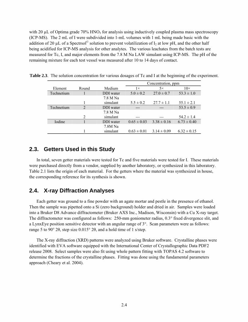
with 20 µL of Optima grade 70% HNO3 for analysis using inductively coupled plasma mass spectroscopy (ICP-MS). The 2 mL of I were subdivided into 1-mL volumes with 1 mL being made basic with the addition of 20 µL of a Spectrsol© solution to prevent volatilization of I2 at low pH, and the other half being acidified for ICP-MS analysis for other analytes. The various leachates from the batch tests are measured for Tc, I, and major elements from the 7.8 M Na LAW simulant using ICP-MS. The pH of the remaining mixture for each test vessel was measured after 10 to 14 days of contact.

Table 2.3. The solution concentration for various dosages of Tc and I at the beginning of the experiment.

Element Round Medium Concentration, ppm

1× 5× 10× Technetium 1 DDI water 5.0 ± 0.2 27.0 ± 0.7 53.3 ± 1.0

1 7.8 M Na simulant 5.5 ± 0.2 27.7 ± 1.1 55.1 ± 2.1

Technetium 2 DDI water --- --- 53.5 ± 0.9

2 7.8 M Na simulant --- --- 54.2 ± 1.4

Iodine 1 DDI water 0.65 ± 0.03 3.38 ± 0.16 6.73 ± 0.40

1 7.8M Na simulant 0.63 ± 0.01 3.14 ± 0.09 6.32 ± 0.15

2.3. Getters Used in this Study

In total, seven getter materials were tested for Tc and five materials were tested for I. These materials were purchased directly from a vendor, supplied by another laboratory, or synthesized in this laboratory. Table 2.1 lists the origin of each material. For the getters where the material was synthesized in house, the corresponding reference for its synthesis is shown.

2.4. X-ray Diffraction Analyses

Each getter was ground to a fine powder with an agate mortar and pestle in the presence of ethanol. Then the sample was pipetted onto a Si (zero background) holder and dried in air. Samples were loaded into a Bruker D8 Advance diffractometer (Bruker AXS Inc., Madison, Wisconsin) with a Cu X-ray target. The diffractometer was configured as follows: 250-mm goniometer radius, 0.3° fixed divergence slit, and a LynxEye position sensitive detector with an angular range of 3°. Scan parameters were as follows: range 5 to 90° 2θ, step size 0.015° 2θ, and a hold time of 1 s/step.

The X-ray diffraction (XRD) patterns were analyzed using Bruker software. Crystalline phases were identified with EVA software equipped with the International Center of Crystallographic Data PDF2 release 2008. Select samples were also fit using whole pattern fitting with TOPAS 4.2 software to determine the fractions of the crystalline phases. Fitting was done using the fundamental parameters approach (Cheary et al. 2004).

2.5

2.5. Specific Surface Area

Surface area, porosity, and pore size analyses were performed on each getter using the N2 adsorption/desorption Brunauer–Emmett–Teller (BET) method (Brunauer et al. 1938). Data were collected with a QUANTACHROME AUTOSORB 6-B gas sorption system. The getter samples were degassed at 25 °C for 8−16 hours under vacuum. The degassed samples were contacted by nitrogen to measure adsorption and desorption at a constant temperature, 77.4K. The BET method is well known and is given by:

)(

11

)( ommOa P

P

CV

C

CVPPV

P

(2.2)

where Va = the quantity of gas adsorbed at pressure, P, Vm = the quantity of gas adsorbed to form a complete monolayer, Po = the saturation pressure of the gas, and C = the BET constant.

2.6

Table 2.1. List and origin of the getter materials used in the experiment.

Targeted Element Getter Full Name

Theoretical Chemical Formula Origin

Vendor Name (if applicable)

Reference (if applicable)

Tc BFS1 Blast Furnace Slag 1 Vendor Lafarge North America

Tc BFS2 Blast Furnace Slag 2 Vendor Holcim (US) Inc.

Tc Tin Apatite Tin(II) Apatite Sn5(PO4)3(F,Cl,OH) Outside Laboratory

Duncan et al. (2009)

Tc SnCl2 --- SnCl2 Vendor Sigma Aldrich

Tc Nano Sn-P Nano Tin Phosphate SnPO4 This Laboratory Wellman et al. (2006)

Tc KMS Potassium Metal Sulfide Outside Laboratory

Mertz et al. (2013)

Tc Sn-HA Tin(II) Hydroxyapatite Sn5(PO4)3(OH) Outside Laboratory

I LBH Layered Bismuth Hydroxide

Bi(OH)3 This Laboratory Krumhansl et al. (2006)

I Argentite --- Ag2S Vendor David K. Joyce Minerals

I Argentite, synthetic --- Ag2S This Laboratory Kaplan et al. (2000)

I Ag Carbon Silver-impregnated carbon Vendor Prominent Systems, Inc.

I Ag Zeolite Silver-exchanged zeolite Vendor Aldrich

2.7

The values of Vm and C are determined by a regression line of the adsorption isotherm plotted with P/Va(Po-P) vs. P/Po. The specific surface area of a solid is determined by:

201022414

Amm Na

VArea

(2.3)

where am is the average area occupied by a single adsorbate molecule, and NA is Avogadro’s number (Gregg and Sing 1982; Webb and Orr 1997). The surface area was determined from the isotherm using a five-point BET method. The BJH method was used for the porosity and pore size analyses; the T method was used for micro pore analyses.

2.6. Moisture Content and Liquid Phase Analyses

The gravimetric water contents of the getter materials were determined using Pacific Northwest National Laboratory (PNNL) procedure PNL-MA-567-DO-1 (PNL 1990). This procedure is based on the American Society for Testing and Materials (ASTM) procedure Test Method for Laboratory Determination of Water (Moisture) Content of Soil and Rock (ASTM D2216-98 [ASTM 1998]). Depending on the availability of the getter, a 0.1- to 1.0-g sample was placed in a tared container, weighed, and dried in an oven at 105 C (221F) for 24 hours. Moisture content measurements were run in triplicate. The containers then were removed from the oven, cooled, and weighed. The containers were then placed back into the oven at 105 C for another 24 hours to ensure that all of the moisture had been removed. All weights of samples were measured using a calibrated balance. A calibrated weight set was used to verify balance performance before weighing the samples. The gravimetric water content was computed as the percentage change in getter mass before and after oven drying.

The pH of each batch effluent solution was measured after 10 to 14 days of contact. Measurements were performed in the anoxic chambers on the bulk solution. The pH was measured with a pH meter calibrated with buffers at pH 4, 7, 10, and 13, and systematic verification of electrode performance was performed after each 10 measurements using the calibration standard with a pH closest to the pH of the samples.

Technetium-99 and iodine-127 analysis for the batch Kd effluents was performed using ICP-MS and high-purity calibration standards to generate calibration curves and verify continuing calibration during the analysis run. Dilutions (from 20×to 500×) were made for each batch Kd effluent from the deionized water (DIW) tests and (500×to 5000×) for analysis of the batch Kd effluents from the 7.8 M Na Ave simulant tests to investigate and correct for matrix interferences. The method used was PNNL-AGG-415 (PNNL 1998), which is quite similar to EPA Method 6020 (EPA 2000).

3.1

3.0 Results and Discussion

In this section of the report we present data from a series of measurements, such as moisture content, surface area, and XRD analyses, as well as data from batch experiments conducted at PNNL to evaluate Tc and I getter performance.

3.1 Moisture Content and Surface Area

Moisture content and surface area data for the various getters are presented in Table 3.1. The values for moisture content are given as an average of three measurements along with the standard deviation (1σ). The moisture content data were used to calculate the dry weight of the sample that is then used to calculate Kd.

The majority of the getters have a moisture content that is less than 2% of the as-received getter mass (Table 3.1). The samples with moisture contents larger than this were KMS, Ag C, and Sn(II)-treated apatite. For the case of Sn apatite more than half of the sample mass was composed of water. The specific surface area (m2/g) of the getters is also shown in Table 3.1. These values were obtained to ascertain if calculated Kd values (reported on a mass basis) were a function of the specific surface area of the getter material.

Table 3.1. Moisture content and surface area of the 12 getters used in testing.

Getter % Average

Moisture Content Standard

Deviation, σ BET Surface

area, m2/g

BFS1 0.99 0.06 1.9 BFS2 0.19 0.02 2.1 SnCl2 0.51 0.14 0.06(a)

Sn(II) Apatite 66.78 0.36 104.8 Sn-HA 1.66 0.33 80.8 KMS 5.48 0.38 5.1

Nano Sn-P 0.40 0.11 4.8 LBH 0.51 0.08 3.9

Argentite 1.03 0.35 0.5a Syn Arg 0.09 0.09 1.1

Ag C 9.05 0.33 1193 Ag zeolite -2.24 0.04 309.5

(a) BET surface area is a maximum value due to the low surface area of these materials requiring an excess of sample.

3.2 X-ray Diffraction Analyses

XRD analyses were conducted with each getter material (as received), before contact with the solution containing either Tc or I. All of the individual diffractograms are presented in Appendix B. Where applicable, diffractograms are given both as raw spectra and with a background subtraction. The

3.2

materials received directly from an industrial supplier (SnCl2, Ag C, and Ag zeolite) showed the expected diffractograms and are not discussed here.

Because of the large variety of getter materials with different chemical formula and structures, the diffractograms vary widely; therefore, comparison between different getter materials is often not possible. The two exceptions are argentite and synthetic argentite, and Sn(II) apatite and Sn(II) hydroxyapatite. For the two argentite minerals, a natural mineral and one synthesized in the laboratory, the two spectra seem to be nearly identical and match Ag2S from the Pattern Diffraction File (PDF) database. For the Sn(II) apatite and Sn(II) hydroxyapatite the patterns show similar peak locations with some differences. The Sn(II) hydroxyapatite seems to be more pure and the results show that this material is a mixture of hydroxyapatite (Ca5(PO4)3OH,syn) and Sn(IV) oxide. In the Sn(II) apatite diffractogram, the broad peaks belong to an apatite structure. The red peaks fit several different chemistries but they fit a Ca1.12Sr1.88 Al2O6 structure most closely. The phase depicted in light blue appears to be a salt, either NaCl or AgBr. At this point we do not have access to the synthesis procedure used to make this material, so we do not know if the presence of these two salts is reasonable. Nevertheless, the two structures are the best fit to the diffractogram. A Sn(II) oxide fits a few of the peaks but is not very prevalent.

Three of the materials, which have been investigated previously, can be compared with XRD patterns available from other studies: BFS1 (Northwest), BFS2 (Southeast), and LBH (layered bismuth hydroxide). The two BFS materials were examined by Westsik et al. (2013). Figure 4.1 from that study shows the Northwest material has several peaks, suggesting crystalline phases are present, while the Southeast material is highly amorphous with an ill-defined peak near 30° 2θ. A similar amorphous peak was observed in the present study, as was a very low intensity peak that matched a Y2O3 PDF. Due to the low intensity of this peak relative to background, a clear identification was not possible. For the Northwest BFS, the Westsik et al. (2013) study identified the peaks in the Northwest BFS as gypsum (CaSO4·2H2O) and bassanite (2CaSO4·H2O). The same two phases were also identified in the present study along with quartz (SiO2), calcite (CaCO3), calcium sulfate (CaSO4), and lithium molybdenum oxide (Li2MoO3)— the last three of these being seemingly minor phases. The previous study may not have been able to identify these phases because it used a 1 s/step dwell time, while a 2 s/step dwell time was used here.

The LBH getter material was investigated by a group at Sandia National Laboratory (Krumhansl et al. 2006). The aim of that study was to create a LBH based on the advantageous properties of the layered double hydroxide materials, hydrotalcite [theoretical formula (Mg6Al2(CO3)(OH)16·4(H2O)], and their ability to sequester anions. Using bismuth also yields the advantage that the metal is not on the Resource Conservation and Recovery Act (RCRA) list. Originally the intent was to dope the LBH material with various alkali metals, but it is unclear from the report whether they were successful. The synthesis of the various LBH materials doped with alkali metals yielded three types of material that were differentiated based on their different XRD patterns. In the Krumhansl et al. (2006) report these three materials were called Type I, II, and II, with the only difference in their performance being that the Type II materials work better for perrhenate, perchlorate, and iodate. For the present report, the LBH getter material was synthesized in our laboratory and we were able to alter the synthesis and create two of the structure types shown in the report by Krumhansl et al. (2006). The pattern for the LBH synthesized material used in this study is given in Appendix B and is predominantly Type I with traces of Type II, when compared with the Krumhansl et al. (2006) nomenclature. Here, we have fit the Type II structure to a bismutite [Bi2(CO3)O2] pattern. The Type I pattern is not available in the PDF library, but the unit cell has been

3.3

indexed successfully and the structure could be identified if the exact chemistry of the material were known.

We can also compare the XRD results obtained here with the potassium metal sulfides (KMSs) material obtained from a research group at Northwestern University. The group is creating a series of KMSs where the substitution of a different metal gives rise to a different material. We were given KMS-2, which has the formula K2xMgxSn3−xS6 (x = 0.5−1) (Mertz et al. 2013). The getter has shown the capacity to incorporate Cs+, Sr2+, and Ni2+ into to a cation monolayer that exists between Sn/MgS6 monolayers. It is thought that the pertechnetate anion will be reduced by the sulfide ions to Tc(IV) that can then replace potassium in the disordered monolayer. The diffractogram obtained in our study is similar to the pattern in Mertz et al. (2013) study but a few minor peaks are also present. However, the dominant peak near 11° 2θ is similar in both diffractograms.

Lastly, the diffractogram for Sn-P, which was synthesized in our laboratory, was fit using a combination of a tin phosphate (Sn2P2O7), a tin hydroxide (Sn0.9(O1.6(OH)0.4), and a large organic molecule that is most likely left over from the synthesis. Unfortunately, the oxidation state of the Sn in the hydroxide is 4+ and thus the material has lost its reducing capacity. The starting material, where tin was in the 2+ state (SnCl2), was probably oxidized to the 4+ state when the material was calcined. The synthesis procedure given by Wellman et al. (2006) did not indicate that the material was calcined under vacuum or in reducing conditions, but it is believed that calcining under such conditions would have yielded the desired material. The experiments had already been initiated by the time the XRD patterns were obtained so it was too late to correct this problem.

3.3 Technetium Getter Distribution Coefficients

It is known that the pH of the solution may have an effect on the performance of the various getter materials. The pH data for the various effluents collected are given in the Appendix C. The final pH of the contacting solution, in most cases, is dictated by the type of getter material, which creates a pH that varies from acidic (SnCl2) to basic (BFS1 and 2). No attempt was made to buffer the deionized distilled (DDI) water solutions so, although pH may play a role in some of the performance of some of the getters, we were not able to elucidate this effect in this set of experiments. Briefly, the goal was to evaluate the performance of the materials in relevant caustic LAW simulants. The DDI water experiments were used mostly to investigate getters performance under ideal conditions where the competition from other aqueous anions (such as chromate and nitrate that are present in the LAQ simulant) is at minimum. The DDI water experiments were also used to compare with previous studies of different getter materials. We also wanted to compare the results from the DDI water experiments with those presented in other previous studies conducted with different getter materials (see discussions in Serne and Westsik 2011), but the experimental conditions in these studies are different from those in our experiments and a good comparison is currently difficult.

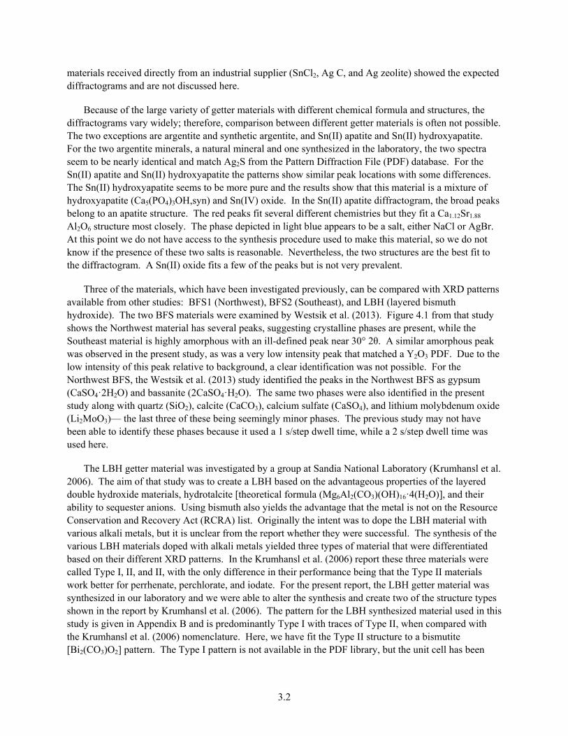
The results of the Tc Kd values for each getter in DDI water and the 7.8 M LAW simulant are shown in Figure 3.1 (C1), Figure 3.2 (C2), and Figure 3.3 (C3). Beginning with Figure 3.1, it is seen that Sn apatite has the best performance in DIW. However, the BFS2 performance seems to be approaching that of tin apatite at the longer time periods. In fact, for both BFS materials the performance of the material seems to be time dependent, i.e., kinetically controlled. It is unclear at this time whether the two BFS materials will reach an equilibrium, or steady-state final Tc concentration, in the effluent like tin apatite

3.4

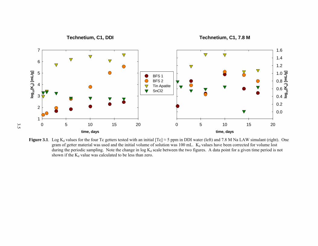
and SnCl2 seem to have done. When more Tc is present in the DDI water solution, as seen in Figure 3.2, the Tc-getter performance of tin apatite seems to improve while the other three getters have lower Tc Kd values. This observation suggests that the apparent reduction of Tc(VII) by the getter material becomes limited by the amount of solid present for these getters. When even more Tc is added (Figure 3.3) the same trend is observed where the performance of Sn apatite increases while the other three getters’ ability to remove Tc decreases, thus supporting the limited available site or limited available reductant hypotheses. In fact, from Table 3.1 it is seen that the surface area of tin apatite is anywhere from 65×–350× greater that the other getter materials so if we assume a similar method of Tc removal for the four getters, the surface area becomes a factor. Knowledge of the reduction capacity of each getter material on a per gram basis would also aid in determining the reason for this difference.

Figure 3.3 also shows the performance of the getters Nano Sn-P, KMS, Sn-HA, and BFS1 at a getter mass to solution volume ratio of 1:10. Of these four getter material tests, the BFS1 at 1:10 has a Tc Kd value that is more than 5 orders of magnitude greater than the Kd for the BFS1 at 1:100. All of the materials in this second suite of tests appear to have reached equilibrium with respect to Tc removal in the system. This result of using BFS1 at two solid-to-solution ratios indicates that the performance of this material is proportional to this getter:Tc mass ratio. Overall, the order of performance at removing Tc(VII) from DDI water is Sn(II)-treated apatite>SnCl2>Nano Sn-P, KMS, BFS2>BFS1, Sn-HA, where we are only comparing samples with the same getter-to-solution ratio.

In each figure, the Kd values measured from experiments conducted with the 7.8 M Na LAW simulant are also given. For C1 and C2 (Figure 3.1 and Figure 3.2, respectively), the four getters show no, to a very small, capacity to remove Tc from the LAW simulant. The reasons for this may be the competing metals in the LAW solution that are more easily reduced than Tc (e.g., Cr(VI). A pH or ionic strength effect is also a possibility. However, three of the getters show some positive results in the highly caustic simulant: KMS, Sn-HA, and Sn(II)-treated apatite. Surprisingly, the KMS and Sn-HA perform better in the 7.8 M LAW simulant than in DDI water. It is unclear why this is true at this point in the experimentation. However, we may look at the chemical structure of the getters to try to elucidate why these two getters perform better under these conditions. When comparing Sn-HA to Sn(II)-treated apatite one should realize that although these two materials are considered both to be tin phosphates, their chemical compositions is different because the hydroxyapatite has only hydroxyl anions present in its crystal structure, whereas tin apatite has F and Cl in addition to the hydroxyl anions. It would be prudent to study the structure, both before and after contact with the caustic LAW simulant, more carefully to see if further insight may be gained. As for KMS, this material contains sulfur in its reduced form (S2-). These sulfide groups may also be donating electrons to Tc(VII) to reduce it to Tc(IV).

3.5

Figure 3.1. Log Kd values for the four Tc getters tested with an initial [Tc] ≈ 5 ppm in DDI water (left) and 7.8 M Na LAW simulant (right). One gram of getter material was used and the initial volume of solution was 100 mL. Kd values have been corrected for volume lost during the periodic sampling. Note the change in log Kd scale between the two figures. A data point for a given time period is not shown if the Kd value was calculated to be less than zero.

Technetium, C1, 7.8 M

time, days

0 5 10 15 20

log

10(K

d)

[mL

/g]

0.0

0.2

0.4

0.6

0.8

1.0

1.2

1.4

1.6

Technetium, C1, DDI

time, days

0 5 10 15 20

log

10(K

d)

[mL

/g]

1

2

3

4

5

6

7

BFS 1 BFS 2 Tin Apatite SnCl2

3.6

Figure 3.2. Log Kd values for the four Tc getters tested with an initial [Tc] ≈ 27 ppm in DDI water (left) and 7.8 M Na LAW simulant (right). One gram of getter material was used and the initial volume of solution was 100 mL. Kd values have been corrected for volume lost during the periodic sampling. Note the change in log Kd scale between the two figures. A data point for a given time period is not shown if the Kd value was calculated to be less than zero.


time, days

0 5 10 15 20

log

10(K

d)

[mL

/g]

0.0

0.5

1.0

1.5

2.0

2.5

Technetium, C2, DDI

time, days

0 5 10 15 20

log

10(K

d)

[mL

/g]

0

2

4

6

8

BFS 1 BFS 2 Tin Apatite SnCl2

3.7

Figure 3.3. Log Kd values for the eight Tc getters tested with an initial [Tc] ≈ 53 ppm in DDI water (left) and 7.8 M Na LAW simulant (right). One gram of getter material was used and the initial volume of solution was 100 mL except for the case of BFS1 1:10 where 10 g of getter were used with 100-mL solution. Kd values have been corrected for volume lost during the periodic sampling. Note the change in log Kd scale between the two figures. A data point for a given time period is not shown if the Kd value was calculated to be less than zero.


time, days

0 5 10 15 20

log

10(K

d)

[mL

/g]

-1

0

1

2

3

4

Technetium, C3, DDI

time, days

0 5 10 15 20

log

10(K

d)

[mL

/g]

-2

0

2

4

6

8

BFS 1BFS 2Tin Apatite SnCl2 Nano Sn-P KMS Sn-HA BFS 1 1:10

3.8

3.4 Iodine Getters Distribution Coefficients

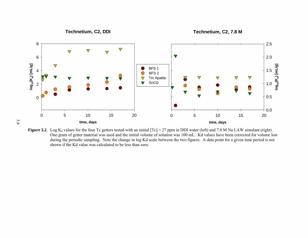
The distribution coefficients for the five iodine getter materials at the three different initial iodide concentrations (0.6, 3, 6 ppm) that were tested are shown in Figure 3.4, Figure 3.5, and Figure 3.6, respectively. In the C1 case in DDI water (Figure 3.4), the iodide Kd values increase in the following order: Argentite<Ag zeolite<LBH<Ag C<Syn Arg. All getters seem to reach an apparent equilibrium with the various materials after 9 days of contact time. An argument could be made that the Ag zeolite iodide Kd value is still increasing. The iodide Kd value for Ag C seems to be dropping after 9 days, but the values are based on iodide concentrations measured very near the Estimated Quantitation Limit (EQL), so even seemingly minor changes in concentrations have a relatively significant effect on the calculated Kd value. The iodide Kd values for Syn Arg at 9 days and beyond are lower limits calculated based on the EQL of the sample.

For the C2 and C3 experiments, the effectiveness of the getters follows the same order as for the C1 samples except for the Ag zeolite getter seems to have a higher Kd value than LBH as the starting iodide concentration increases. Another interesting trend observed as the starting iodide concentration increases is that the Syn Arg C3 sample iodide Kd values seem to be increasing throughout the 15-day contact period. We did not observe this trend for the two lower starting iodide concentrations because the effluent iodine concentrations for those batch adsorption tests were below the EQL. Therefore, we are only able to establish a lower limit for Kd for the Syn Arg getter in DDI water. Also, we note that the Kd value of Ag zeolite increases with increasing starting iodide concentration. This may be due to its high surface area and possibly slow kinetics that do not allow iodine to find sorption/precipitation sites on the zeolite surface. It should be noted that the other getter with a very high surface area, Ag C, does not show an increase of Kd with surface area, suggesting that the material is in apparent equilibrium with I in the system.

When considering the different getters in the 7.8 M LAW simulant, two getters are much more effective than the others: Ag zeolite and Syn Arg. The other getters have calculated iodide distribution coefficients that show very limited effectiveness in the caustic conditions created by the LAW simulant. On the other hand, the Ag zeolite iodide Kd values that are given are lower limits because the iodide concentrations in the effluents fall below the EQL after the first sampling. A second experiment using C3 and Ag zeolite in the 7.8 M solution was run to confirm this effect. Effluent samples were taken over shorter time periods and the removal of iodide from solution seems to be confirmed.

3.9

Figure 3.4. Log Kd values for the five I getters tested with an initial [I] ≈ 0.6 ppm in DDI water (left) and 7.8 M Na LAW simulant (right). One gram of getter material was used and the initial volume of solution was 100 mL. Kd values have been corrected for volume lost during the periodic sampling. Vertical arrows indicate that the Kd value was calculated based on the iodide EQL for the effluent sample. Note the change in log Kd scale between the two figures. A data point for a given time period is not shown if the Kd value was calculated to be less than zero.

Iodine, C1, 7.8 M

time, days

0 5 10 15 20

log

10(K

d)

[mL

/g]

-1

0

1

2

3

4

Iodine, C1, DDI

time, days

0 5 10 15 20

log

10(K

d)

[mL

/g]

1.0

1.5

2.0

2.5

3.0

3.5

4.0

4.5

5.0

LBHArgentiteAg CAg zeoliteSyn Arg

3.10

Figure 3.5. Log Kd values for the five I getters tested with an initial [I] ≈ 3 ppm in DDI water (left) and 7.8 M Na LAW simulant (right). One gram of getter material was used and the initial volume of solution was 100 mL. Kd values have been corrected for volume lost during the periodic sampling. Vertical arrows indicate that the Kd value was calculated based on the iodide EQL for the effluent sample. Note the change in log Kd scale between the two figures. A data point for a given time period is not shown if the Kd value was calculated to be less than zero.

Iodine, C2, 7.8 M

time, days

0 5 10 15 20

log

10(

Kd)

[mL

/g]

-2

-1

0

1

2

3

4

5

Iodine, C2, DDI

time, days

0 5 10 15 20

log

10(

Kd)

[mL

/g]

0

1

2

3

4

5

6


3.11

Figure 3.6. Log Kd values for the five I getters tested with an initial [I] ≈ 6 ppm in DDI water (left) and 7.8 M Na LAW simulant (right). One gram of getter material was used and the initial volume of solution was 100 mL. Kd values have been corrected for volume lost during the periodic sampling. Vertical arrows indicate that the Kd value was calculated based on the iodide EQL for the effluent sample. Note the change in log Kd scale between the two figures. A data point for a given time period is not shown if the Kd value was calculated to be less than zero.

Iodine, C3, 7.8 M

time, days

0 5 10 15 20

log

10(

Kd)

[mL

/g]

-1

0

1

2

3

4

5

Iodine, C3, DDI

time, days

0 5 10 15 20

log

10(

Kd)

[mL

/g]

0

1

2

3

4

5

6

7


3.12

3.5 Behavior of I and Tc at Periods Longer than 15 Days

An extended leaching sample (i.e., the contact time being greater than 15 days) has also been taken to study time-dependent trends at a longer experimental time. Results are presented in the Appendix C and these results are discussed briefly here.

The BFS1 material Tc removal from the DDI water accelerated compared to the quasi-linear removal rate observed for the first 15 days. In fact, for the BFS1 C1 sample, the aqueous Tc concentration dropped below the detection limit indicating full removal. For the BFS2 samples, all 35-day sampling results show values below the EQL. Another getter that showed significant changes during the period between 15 and 35 days was Sn-HA, where Tc values plummeted from near initial concentration levels to below the detection limit (Kd from ~5 to >2.0 × 105). For the SnCl2 getter, effluent Tc concentrations also seemed to drop steadily with reaction time. On the other hand, Tc concentrations, and therefore Kd values, for Nano Sn-P, KMS, and BFS1 1:10 batch sorption tests remained unchanged. The DDI water blank solution Tc concentrations did not vary outside of expected instrumental error, showing that no precipitation of Tc or sorbing onto the container walls occurred during the entire 35-day time period.

For the experiments conducted with the 7.8 M LAW simulant, the majority of the supernate samples showed very small decreases in Tc concentrations for the 35-day samplings compared to the 15-day samplings. However, the Tc concentration in the blanks also dropped slightly during this period. The behavior of Sn-HA was unexpected because this material removed Tc from solution in the first 15 days, but Tc was released again in the time interval 15−35 days (the 35-day Kd value was 10× lower than the 15-day Kd ). The reason for this behavior remains unknown. It was also observed that the BFS1 1:10 test shows a slow but steady decrease in aqueous Tc throughout the 35-day contact time. At the end of 35 days, about 20% of the original Tc had been removed from solution. The highest Kd value for Tc in these sets of experiments was calculated for the KMS getter at 35 days where Kd values were about 104 mL/g.

A 46-day sample was taken in the experiments conducted with I getters. For the samples in the presence of DDI water and the 7.8 M LAW simulant, all of the I solution concentrations remained relatively unchanged. The only getter showing a relatively significant change in the concentration of I was synthetic argentite where a continuous decrease in the concentration of I was observed. In fact, for the experiments conducted with the C1 and C2 I concentrations, the I concentration was below the EQL. Both Ag zeolite and synthetic argentite demonstrated very promising performance in the highly caustic 7.8 M LAW simulant.

3.6 Normalization of Kd Values with the Surface Area

It has been suggested here that the mechanism responsible for Tc removal from solution is a redox reaction where Tc(VII) is converted to the less soluble Tc(IV) and I is thought to precipitate with available Ag ions to form AgI (however, this would not be the case for LBH, which relies on anionic substitution in the interlayer sites). To investigate the surface area effect, we plotted the specific surface area of each getter versus the Kd value for the C3 concentrations only in DDI water for the 15-day sample. We did not examine the surface area effect for the LAW simulant solutions because of the general poor performance of all getters in these solutions. For the Tc getters, a correlation between the surface area of the material and the Kd value does not seem to exist. The change in the BET surface area when 10× more

3.13

BFS1 material is used in the BFS1 1:10 test (as opposed to the BFS1 test) does not correspond to a 10× increase in the Kd value. In fact, the Kd increase is about 8 orders of magnitude greater. Therefore, the surface area of each Tc-getter material does not appear to control its capacity to remove Tc from solution.

The corresponding relationship between I getter performance and surface area revealed a relatively linear increase in the Kd value with increasing surface area for four of the five getters. Synthetic argentite, which has the largest 15-day Kd value, falls off of this line. It was previously observed (Figure 3.6) that the Kd value increases with time for synthetic argentite, suggesting that the synthetic argentite continues to dissolve in solution with time thus freeing available silver ions that may react and co-precipitate with iodide.

3.7 Behavior of Other Elements Present in the Simulant

One of the possible reasons for the decreased performance of the Tc getters in the 7.8 M Na LAW simulant may be competition from other ions present in the simulant that may react with the getter material more readily than the Tc and thus consume some of the reduction capacity of the material. To demonstrate this competition we used Cr as an example because it is a redox-sensitive element with the highest concentration (about 1700 ppm measured by ICP-MS; Table 3.2 and Table 3.3). Because it takes three electrons to reduce Cr(VI) to Cr(III), approximately 10 meq of reductant are needed to reduce all of the Cr present in 100 mL of the 7.8 M Na LAW simulant. By comparison, only 0.015 and 0.167 meq are needed to reduce the Tc(VII) present in 100 mL for the C1 and C3 tests, respectively. The reduction capacity for BFS1 and BFS2, which was measured using the Ce(IV) methodology of Angus and Glasser (1985), was 0.793 and 0.800 meq/g [Um et al. (2012, 2013)], and 0.884 and 0.725 meq/g [Langton et al. (2013)],2 respectively. Because only 1 g of getter material was used in the experiments conducted at a 1:100 getter-to-LAW simulant ratio, there was insufficient reduction capacity to reduce all of the Cr and Tc present in the LAW simulant. Some of the Cr may have been reduced during these experiments (the concentrations of Cr decreased with time in some experiments as is shown in the data presented in Tables 3.2 and 3.3). However, only a few of the Tc-getter materials removed Cr from the 7.8 M LAW simulant with KMS and BFS1 (1:10 ratio) showing the largest decrease in the Cr concentration compared to the blank. In addition, the highest Tc Kd values were measured in experiments conducted with these two materials (i.e., KMS and BFS1), which suggests either partial or insignificant Cr competition, and definitely calls into question the hypothesis that Cr competition is the cause of poor getter performance in the presence of the 7.8 M Na LAW simulant. Further investigations are definitely warranted in this area. The reduction capacity for the other materials used as getters is unknown at this time.

Although the reductive capacity is not considered an issue for the removal of I from solution it is nevertheless instructive to perform a similar analysis of three RCRA metals (Cr, Cd, and Pb) to see if they are also removed from the 7.8 M Na Ave simulant. As seen in Table 3.4, Ag zeolite removes approximately 99% of Cr, and 93% of Cd and Pb after 15 days. These results are encouraging because this getter material also shows very promising performance in terms of I removal. LBH is very effective at removing Pb from solution with more than 99% of the element being removed after 0.2 days of contact time.

2 Langton CA. 1988. “Challenging Applications for Hydrated and Chemical Reacted Ceramics.” DP MS 88-163, presentation given at American Ceramic Society Meeting, Sydney, Australia, July 12, 1988.

3.14

Table 3.2. Concentration of Cr in the LAW simulant effluents from Tc batch tests at 0.2 and 15 days for various getters. The blank was sampled at the same time as the getter materials listed in the table.

Time, days

[Cr] Concentration,ppm

Average Stdev

Tc BLK6 0.2 1710 42 15 1685 7 BFS1 0.2 1740 85 15 1680 156 BFS2 0.2 1880 0 15 1760 42 Tin apatite 0.2 1555 49 15 1515 7 SnCl2 0.2 1085 64 15 1035 50

Table 3.3. Concentration of Cr in the LAW simulant effluents from Tc batch tests at 0.2 and 15 days for various getters. The blank was sampled at the same time as the getter materials listed in the table.

Time, days

[Cr] Concentration,ppm

Average Stdev

Tc BLK12 0.2 1880 14 15 1985 120 Nano Sn P 0.2 1685 7 15 1905 21 KMS 0.2 1550 14 15 1020 0 Sn-HA 0.2 1685 49 15 1670 0 BFS1 1:10 0.2 1720 0.0 15 1215 21

3.15

Table 3.4. Concentration of Cr, Cd, and Pb in LAW Simulant at 0.2 and 15 days for the various getters used in the iodine tests.

Concentration, ppm

Time, days

[Cr] [Cd] [Pb]

Average Stdev Average Stdev Average Stdev

I BLK 0.2 1805 49 13.8 0.2 82.0 2.4 15 1605 78 13.7 0.2 73.8 3.0 LBH 0.2 1785 7 6.2 1.4 0.20 0.0 15 1520 42 1.7 0.2 0.24 0.0 Argentite 0.2 1535 35 6.9 1.8 132 9.2 15 1770 28 3.0 0.9 166 3.5 Ag C 0.2 1785 35 9.8 0.4 66.5 2.1 15 1790 14 9.4 0.2 68.2 1.0 Ag zeolite 0.2 29.8 0.1 7.0 0.2 50.9 2.7 15 35.9 0.4 0.9 0.2 5.2 0.0 Syn argentite 0.2 1690 28 13.5 0.1 76.1 0.2 15 1710 57 14.0 0.8 77.0 1.5

4.1

4.0 Conclusions

To determine the effectiveness of the various getter materials, a series of batch sorption experiments was performed. To quantify the effectiveness of the removal of Tc(VII) and I(I) from solution by getters, the distribution coefficient, Kd (mL/g), was calculated. Testing involved placing 1.0 g of getter material in contact with 100 mL of solution for periods up to 1 month with periodic solution sampling. One Tc getter was tested at a 1:10 solid-to-solution ratio. Two different solution media, 18.2 MΩ DI H2O and a 7.8 M Na Ave waste simulant, were used in the batch sorption tests. Each test was conducted in a 250-mL PTFE bottle at room temperature (~22 °C) in an anoxic chamber containing N2 with a small amount of H2 (0.7%) to maintain anoxic conditions. Each getter-solution combination was run in duplicate. Three Tc- and I-doping concentrations were used separately in aliquots of both the 18.2 MΩ DI H2O and a 7.8 M Na Ave simulant. The 1× concentration was developed based on HTWOS model runs to support the River Protection Project System Plan Revision 6. The other two concentrations were 5× and 10× of the HTWOS values. The Tc and I tests were run separately (i.e., the solutions did not contain both solutes). Sampling of the solid-solution mixtures occurred nominally after 0.2, 1, 3, 6, 9, 12, 15 days, and 1 month. Seven getter materials were tested for Tc and five materials were tested for I. The seven Tc getters were BFS1 (northwest source), BFS2 (southeast source), Sn(II)-treated apatite, Sn(II) chloride, nano tin phosphate, KMS (a potassium-metal-sulfide), and tin hydroxapatite. The five iodide getters were LBH, argentite mineral, synthetic argentitie, silver-treated carbon, and silver-treated zeolite.

Results of the Tc Kd values for each getter in DDI water and the 7.8 M LAW simulant suggest that Sn(II)-treated apatite has the best performance in DDI water. However, the BFS2 (southeast source) performance seems to be approaching that of tin apatite at the longer time periods in contact with DDI water. Both BFS materials performance at removing Tc from DDI water seems to be time dependent, i.e., kinetically controlled. It is unclear at this time if the two BFS materials will reach an equilibrium or steady-state final Tc concentration in DDI water such as happened in the effluents contacting Sn(II)-treated apatite and SnCl2. When more Tc is present in the DDI water solution, the Tc-getter performance of Sn(II)-treated apatite seems to improve while the other Tc getters have lower Tc Kd values. This observation suggests that the apparent reduction of Tc(VII) by the getter material becomes limited by the amount of solid present for these getters. This observation supports the hypothesis that the Tc getters studied have either limited available sites or limited available reducing capacity. Specific surface area measurements show that the Sn(II)-treated apatite has between 65× to 350× greater surface area than the other Tc-getter materials so if we assume a similar method of Tc removal for all the Tc getters, their specific surface area becomes a factor. Three Tc-getter materials (nano tin phosphate, KMS, and tin hydroxapatite) seem to have reached equilibrium with respect to Tc removal in the first 15 days of contact. The BFS1 at the solid-to-solution ratio of 1:10 has a Tc Kd value that is more than 5 orders of magnitude greater than the Kd for its test at the 1:100 ratio in DDI water. This result for using BFS 1 at two solid-to-solution ratios indicates the performance of this material is proportional to the getter:Tc mass ratio. Overall, the order of performance for removing Tc(VII) from DDI water is Sn(II)-treated apatite>SnCl2>Nano Sn-P, KMS, BFS2>BFS1, Sn-HA, where only results for the 1:100 solid-to-solution ratio are compared.

For the Tc Kd values measured from experiments conducted with the 7.8 M Na Ave simulant, the first four getters (BFS1, BFS2, Sn(II)-treated apatite, and Sn(II) chloride) show no, to a very small, capacity to remove Tc from the LAW simulant. Reasons for this observation may be the competing metals in the LAW waste solution that are more easily reduced than Tc [e.g., Cr(VI)]. A pH or ionic strength effect is

4.2

also a possibility. Three other Tc getters (KMS, tin apatite, and tin hydroxapatite) show some Tc removal potential in the highly caustic simulant. Surprisingly, the KMS and Sn-HA perform better in the 7.8 M LAW simulant than in DDI water. The cause for this is unclear at this point in the studyWe will look at the chemical structure of the getters both before and after contact with the LAW simulant in an attempt to elucidate the reason why these two getters perform better under these conditions.

For the Tc-getter tests in DDI water that were re-sampled after 35 days of contact, both BFS materials removed Tc from solution at a significantly greater rate than they did during the first 15 days. In fact, for the BFS1 lowest starting Tc concentration and for all three starting Tc concentrations for the BFS2 samples, all 35-day sampling results show values below the Tc detection limit. Another Tc getter that showed significant drops in Tc solution concentrations during the period between 15 and 35 days was SnCl2. On the other hand, Tc concentrations, and therefore Kd values, for Nano Sn-P, KMS, and BFS1 at concentration ratios of 1:10 remained near where they were after the first 15 days of study.

For the Tc-getter experiments in the 7.8 M LAW simulant, the majority of the effluent samples show very small drops in Tc concentrations for the 35-day compared to the 15-day samplings. However, the Tc concentration in the simulant blanks also dropped slightly during this period, so the effect of the getter contacting LAW simulant at 35 days compared to 15 days is minimal. Also, the Sn-HA sample, which showed some capacity to remove Tc from the LAW simulant through the early experimental times, gives a 35-day Kd value that is 10× lower than the 15-day sample. The reason for this is unknown but may be related to a re-oxidation of Tc. The BFS1 1:10 test shows a slow but steady decrease in Tc supernate concentration in the LAW simulant from 0.2 to 35 days of contact. After 35 days contact about 20% of the original Tc was removed from solution. Lastly, the KMS getter gives the highest Kd value for Tc at 35 days where Kd values have increased to greater than 104 mL/g.

In the C1 case in DDI water (Figure 3.4), the iodide Kd values increase in the following order: Argentite<Ag zeolite<LBH<Ag C<Syn Arg. All getters seem to reach an apparent equilibrium with the various materials after 9 days of contact time. Another interesting trend observed as the starting iodide concentration increases is that the Syn Arg C3 sample iodide Kd values seem to be increasing throughout the 15-day contact period. This trend could not be observed for the two lower starting iodide concentrations because the effluent iodine concentrations for those batch adsorption tests were below the EQL. Therefore, we were only able to only establish a lower limit for Kd for the Syn Arg getter in DDI water. Also, we note that the Kd value of Ag zeolite increases with increasing starting iodide concentration. This may be due to its high surface area and possibly slow kinetics that do not allow iodine to find sorption/precipitation sites on the zeolite surface.

When considering the different getters in the 7.8 M LAW simulant, two getters are much more effective than the others: Ag zeolite and Syn Arg. The other getters have calculated iodide distribution coefficients that show very limited effectiveness in the caustic conditions created by the LAW simulant. A 46-day sample was taken for the getter materials used for I removal from solution. For the samples in the presence of DDI water and the 7.8 M LAW simulant, all of the I solution concentrations remained relatively stable. The only getter showing a relatively significant change in the concentration of I was the synthetic argentite samples where a continuous drop in the concentration of I is observed.

5.1

5.0 Future Studies

The tests and literature review documented herein represent about 6 months of activity completed in the last half of 2013; additional activities are planned to be conducted in the future. We will continue our focused efforts to determine if there is an appropriate getter that when used in Cast Stone formulations will significantly decrease the Tc and I diffusivities and their overall release. To achieve this short-term objective we will work in parallel to answer the question of how and why the getter is effective so that we can assess whether or not will exhibit a good long-term performance. In addition, we will continue working in the future to 1) determine an acceptable formulation for the LAW Cast Stone waste form with getters; 2) demonstrate the robustness of the formulation in terms of Tc and I release diffusivities; and 3) provide Cast Stone contaminant release data for risk assessment evaluations

One of the first activities planned once additional funding is allocated is to measure the reductive capacity of all the other Tc getters using the Angus and Glasser (1985) Ce(IV) method. Recall that this method has been used by scientists at both PNNL and SRNL to evaluate the reduction capacity of the Cast Stone dry blend ingredients, cured Cast Stone, and post-leached Cast Stone. Thus to allow comparisons the same procedure should be used to evaluate the reduction capacity of the other Tc getters.

In addition detailed solid-phase characterization of the getter materials will be performed using synchrotron X-ray absorption spectroscopy (specifically X-ray absorption near-edge spectroscopy [XANES] and extended X-ray absorption fine structure [EXAFS]) and perhaps other state-of-the-art solid-phase characterization tools [e.g., X-ray photoelectron spectroscopy (XPS), X-ray fluorescence (µXRF), and transmission electron microscopy (TEM]. XANES is used to delineate the valence state of key elements such as Tc, Cr, S, Fe, and I in the getter solid matrix. EXAFS is used to evaluate the co-ordination number of these key atoms with other close neighbor major structural atoms that constitute the bulk of the solid phase (Al, Si, O, etc.). EXAFS also allows estimates of the bond lengths between neighboring atoms so that structural information about the solid phase can be inferred. The first samples that will be sent to the synchrotron facility for detailed X-ray absorption characterization will be the Tc loaded getters that sequestered the most Tc from both the DDI water and 7.8 M Na Ave simulant. The loaded Tc getters will be from the batch tests that used the highest starting Tc solution concentrations, 10× or C3 (see Table 2.3 and Appendix C).

Similar solid-phase characterization will be performed on the loaded I getters if preliminary work shows that synchrotron X-ray absorption spectroscopy has adequate sensitivity to measure iodine species in standard iodine reference solids at concentrations calculated to be present in the loaded I getters from our finished batch studies described in Section 3. For the Tc getters, synchrotron X-ray absorption spectroscopy will also characterize sulfur species in the BFS getters and perhaps Sn in the tin-bearing getters. In both instances, the goal will be to evaluate whether there is direct bonding between Tc and either the sulfur or tin atoms in the getters and what the nature of the valence states and structures are for the bonded Tc-S or Tc-Sn compounds.

Other studies contemplated early in this ongoing study include more batch sorption tests using Tc getters contacting Tc-spiked 7.8 M Na Ave simulant without chromate at solid-to-solution ratios of 1:100 and 1:10. The periodic sampling of the supernatant will be performed to evaluate the kinetics of Tc removal by the various getters. A second suite of Tc-getter batch sorption tests using the 7.8 M Na Ave simulant with chromate but without Tc(VII) at solid-to-solution ratios of 1:100 and 1:10 will be

5.2

performed in similar fashion. The goal here will be to evaluate the kinetics of Cr(VI) removal with that of Tc(VII) in the first suite of batch sorption tests.

If these two suites of tests do not yield a good understanding of the kinetics and effectiveness of the Tc getters to reduce/remove Cr(VI) and Tc(VII), then a third suite of batch sorption tests will be performed. The tests will use a simplified high salinity-high caustic simulant (consisting of only sodium nitrate and sodium hydroxide with 1 to 1.5 M “free” hydroxide); only Cr(VI) will be added to one batch and only Tc(VII) will be added to another batch —both at the same milliequivalent. To a third batch of concentrated Na-NO3-OH solution both Cr(VII) and Tc(VII) will be added but at a 50 to 1 excess of Cr(VI) over Tc(VII) in terms of milli-equivalents (this is the ratio for the 7.8 M Na Ave simulant for the high dosage Tc). Similar periodic samplings of supernatant will be performed with the same goal of determining (comparing and contrasting) the kinetics of Cr(VI) and Tc(VII) removal in a very simple solution.

If this third suite of tests with a simpler high salinity-high caustic simulant does not yield a clear understanding of the kinetics of Cr(VI) and Tc(VII) removal then a fourth suite of batch sorption tests for the Tc getters might be performed using a NaCl and NaOH instead of the NaNO3-NaOH as the background electrolyte to be certain that nitrate is not confounding the reduction process.

Once we have gained a good understanding of the efficiency of each getter to remove Tc or I and the kinetic attributes of the getters, the overall project goal is to choose two Tc and two I getters for incorporation into Cast Stone. Assuming that all the batch sorption tests performed to date and described in these future studies allow adequate understanding and a technically based selection of the two “best” getters for each of the two groundwater risk driver contaminants (99Tc and 129I) the following work will be performed.

Based on the results of the batch sorption tests, Cast Stone specimens will be prepared with LAW and secondary waste simulants) spiked with Tc, I, and Cr(VI) (assuming adequate time and funding are available). The first suite of tests will use the 7.8 M Na Ave simulant spiked with Tc, I, and Cr(VI). The decision about whether to add the getter first to the spiked liquid simulant or to the dry blend will be based on the kinetic batch sorption tests. The amount of getter used will be chosen based on the results of kinetic batch sorption tests.

The standard Cast Stone dry blend (8% cement Type I/II, 45% fly ash [NW source] and 47% BFS [NW source]) will be modified by the addition of the getter(s). The mixing ratio of the spiked simulant and dry blend will be 0.6 based on the free water content of the simulant. This mix ratio was chosen to coincide with one of the mix ratios used in the LAW screening tests so that a direct comparison can be made with the screening test leach tests for the three contaminants of interest (I, Tc(VII), and Cr(VI). Standard Cast Stone monoliths 2–in. in diameter by 4–in. long will be manufactured and cured for the standard 28-day period under 100% relative humidity. Duplicate monoliths of each getter combination will be manufactured and leached. Three control Cast Stone monoliths (no getters added) will also be prepared and leached in identical fashion.

Individual 28-day cured Cast Stone monoliths with the selected getters will be immersed in one of two leachants, DIW or simulated Hanford vadose zone pore water at a ratio of 9 cm3 of leachant per square centimeter of monolith geometric surface area. The leach protocol will be static leach testing (no leachant renewal at periodic time intervals such as used in the EPA Method 1315). At leach intervals to

5.3

be specified in a test plan, small aliquots of the leachate supernate will be removed and analyzed for the constituents of interest. The relative concentrations of the contaminants of concern as function of time will give an indication of the effectiveness of the getters present in the Cast Stone monoliths. An equivalent aliquot of fresh DIW will be added to the static leach containers to keep the leachate volume constant. In a second set of Cast Stone with getters present both a Tc and I getter will be present in the monolith to ascertain whether having both getters present together causes any synergistic or antagonistic performance related to the sequestering any of the three contaminants of concern (Tc, I, Cr).

6.1

6.0 References

This list contains references for sources cited in the appendixes as well as in the main text of this report.

Allen PG, GS Siemering, DK Shuh, JJ Bucher, NM Edelstein, CA Langton, SB Clark, T Reich, and MA Denecke. 1997. “Technetium Speciation in Cement Waste Forms Determined by XANES.” Radiochimica Acta 76:77–86.

Angus MJ and FP Glasser. 1985. “The Chemical Environment in Cement Matrices.” In Scientific Basis for Nuclear Waste Management, 13th edition, Volume 50, pp. 547−556. Materials Research Society, Pittsburg, Pennsylvania.

ANSI (American National Standards Institute). 2003. Measurement of the Leachability of Solidified Low Level Radioactive Waste by a Short-Term Test Procedure. ANS16.1, American Nuclear Society, La Grange Park, Illinois.

ASTM (American Society for Testing and Materials). 1998. Test Method for Laboratory Determination of Water (Moisture) Content of Soil and Rock. ASTM D2216-98, American Society for Testing and Materials, West Conshohocken, Pennsylvania.

Brown CF, JH Westsik,Jr, RJ Serne, BM Rapko, WR Wilmarth, DJ McCabe, CA Nash, and AD Cozzi. 2013. Preliminary Assessment of the Low-Temperature Waste Form Technology Coupled with Technetium Removal. PNNL-22103 and SRNL-STI-2013-00002 Rev. 0, Pacific Northwest National Laboratory, Richland, Washington, and Savannah River National Laboratory, Aiken, South Carolina.

Brunauer S, PH Emmett, and E Teller. 1938. “Adsorption of Gases in Multimolecular Layers.” Journal of the American Chemical Society 60:309–319.

Certa PJ, PA Empey, and MN Wells. 2011. River Protection Project System Plan. ORP-11242, Revision 6, Washington River Protection Solutions, LLC, Richland, Washington.

Cheary, RW, AA Coelho, and JP Cline. 2004. “Fundamental Parameters Line Profile Fitting in Laboratory Diffractometers.” Journal of Research of the National Institute of Standards and Technology 109:1–25.

Cooke GA, JH Duncan, and LL Lockrem. 2008. Assessment of Technetium Leachability in Cement-Stabilized Basin 43 Groundwater Brine. RPP-RPT-39195, Rev. 0, CH2M Hill Hanford Group, Inc., Richland, Washington.

Cooke GA, LL Lockrem, MD Guthrie, KJ Lueck, and M Avila. 2006. Development and Testing of a Cement-Based Solid Waste Form Using Synthetic UP-1 Groundwater. RPP-RPT-31740, Rev. 0, CH2M Hill Hanford Group, Inc., Richland, Washington.

DOE 2012. DOE (U.S. Department of Energy). 2012. Final Tank Closure and Waste Management Environmental Impact Statement for the Hanford Site,Richland, Washington (TC &

6.2

WM EIS) DOE/EIS-0391. Office of River Protection, U.S. Department of Energy, Richland, WA. http://www.hanford.gov/page.cfm/FinalTCWMEIS

Duncan JB, Cooke, LL Lockrem, MD Guthrie, and KJ Lueck. 2009. Assessment of Technetium GA Leachability in Cement-Stabilized Basin 43 Groundwater Brine. RPP-RPT-39195, Revision 1, Washington River Protection Solutions, Richland, Washington.

EPA (U.S. Environmental Protection Agency). 2000. Method 6020 “Inductively Coupled Plasma-Mass Spectrometry.” In Test Methods for Evaluating Solid Waste, Physical/Chemical Methods. EPA Publication SW-846, available online http://www.epa.gov/epawaste/hazard/testmethods/index.htm.

Gilliam TM, RD Spence, WD Bostick, and JL Shoemaker. 1990. “Solidification/Stabilization of Technetium in Cement-Based Grouts.” Journal of Hazardous Materials 24:189–197.

Gregg SJ and KSW Sing. 1982. Adsorption, Surface Area, and Porosity. Second edition, Academic Press, Orlando, Florida.

Guthrie MD, GA Cooke, JB Duncan, and LL Lockrem. 2009. Assessment of Pertechnetate Getters, Reductants, and Stabilization. RPP-41321-VA, Revision 0, Washington River Protection Solutions, Richland, Washington.

Harbour JR and AS Aloy. 2007. International Program: Summary Report on the Properties of Cementitious Waste Forms. WSRC-STI-2007-00056, Revision 0, Savannah River National Laboratory, Aiken, South Carolina.

Harbour JR, TB Edwards, T Lorier, CA Langton, RC Moore, JL Krumhansl, KC Holt, F Salas, and CA Sanchez. 2004. Stabilizing Grout Compatibility Study. WSRC-TR-2004-00021, Revision 0, Savannah River National Laboratory, Aiken, South Carolina.

Kaplan DI, SV Mattigod, KE Parker, and G Iversen. 2000. Experimental Work in Support of the 129I Disposal Special Analysis. WSRC-TR-2000-00283, Rev. 0, Westinghouse Savannah River Company, Aiken, South Carolina.

Kaplan DI, K Roberts, J Coates, M Siegfried, and S Serkiz. 2008. Saltstone and Concrete Interactions with Radionuclides: Sorption (Kd), Desorption, and Reduction Capacity Measurements. SRNS-STI-2008-00045, Savannah River National Laboratory, Aiken, South Carolina.

Kobayashi, T, AC Scheubist, D Fellauer, X Gaona, and M Altmaier. 2013. “Redox Behaviour of Tc(VII)/Tc(IV) under Various Reducing Conditions in 0.1 M NaCl Solutions.” Radiochim. Acta 101:322-332.

Krumhansl JL, JD Pless, B Chwirka, and KC Holt. 2006. Yucca Mountain Project Getter Program Results (Year 1): I-129 and Other Anions of Concern. SAND2006-3869, Sandia National Laboratories, Albuquerque, New Mexico.

Krupka KM, RJ Serne, and DI Kaplan. 2004. Geochemical Data Package for the 2005 Hanford Integrated Disposal Facility Performance Assessment. PNNL-13037, Rev. 2, Pacific Northwest National Laboratory, Richland, Washington.

6.3

Langton CA and PM Almond. 2013. Cast Stone Oxidation Front Evaluation: Preliminary Results for Samples Exposed to Moist Air. SRNL-STI-2013-00541, Revision 0, Savannah River National Laboratory, Aiken, South Carolina.

Lockrem LL. 2005. Hanford Containerized Cast Stone Facility Task 1-Process Testing and Development Final Report. RPP-RPT-26742, Revision 0, CH2M Hill Hanford Group, Inc., Richland, Washington.

Lockrem LL, GA Cooke, BA Clark, and R West. 2005. Cast Stone Technology for Treatment and Disposal of Iodine-Rich Caustic Waste Demonstration-Final Report. RPP-RPT-26725, Revision 0, CH2M Hill Hanford Group, Inc., Richland, Washington.

Lukens WW, JJ Bucher, DK Shuh, and NM Edelstein. 2005. “Evolution of Technetium Speciation in Reducing Grout.” Environmental Science & Technology 39:8064–8070.

Mahoney LA and RL Russell. 2004. Vitrification Offgas Caustic Scrubber Secondary Waste Simulant Formulation. PNNL-14582, Revision 1, Pacific Northwest National Laboratory, Richland, Washington. Mann FM, RJ Puigh, SH Finfrock, EJ Freeman, R Khaleel, DH Bacon, MP Bergeron, BP McGrail, SK Wurstner, K Burgard, WR Root, and P LaMont. 2001. Hanford Immobilized Low-Activity Tank Waste Performance Assessment: 2001 Version. DOE/ORP-2000-24 Rev. 0, Office of River Protection, U.S. Department of Energy, Richland, Washington.

Mann FM, RJ Puigh, R Khaleel, S Finfrock, BP McGrail, DH Bacon, and RJ Serne. 2003. Risk Assessment Supporting the Decision on the Initial Selection of Supplemental ILAW Technologies. RPP-17675, Revision 0, CH2M Hill Hanford Group Inc., Richland, Washington.

Mattigod SV, RJ Serne, and GE Fryxell. 2003. Selection and Testing of “Getters” for Adsorption of Iodine-129 and Technetium-99: A Review. PNNL-14208, Pacific Northwest National Laboratory, Richland, Washington.

Mattigod SV, JH Westsik, Jr., CW Chung, MJ Lindberg and KE Parker. 2011a. Waste Acceptance Testing of Secondary Waste Forms: Cast Stone, Ceramicrete and DuraLith. PNNL-20632, Pacific Northwest National Laboratory, Richland, Washington.

Mattigod SV, JH Westsik, Jr, and DM Wellman. 2011b. “Evaluation and Selection of 99Tc Getters for Sequestration of Liquid Secondary Wastes Resulting from Vitrification of Radioactive Wastes from Hanford.” Paper 11167, WM2011 Conference, February 27–March 3, 2011, Phoenix, Arizona. Accessed on January 27, 2014 at http://www.wmsym.org/archives/2011/papers/11167.pdf.

Mertz JL, ZH Fard, CD Malliakas, MJ Manos, and MG Kanatzidis. 2013. “Selective Removal of Cs+, Sr2+, and Ni2+ by K2xMgxSn3−xS6 (x = 0.5−1) (KMS-2) Relevant to Nuclear Waste Remediation.” Chemistry of Materials, 25:2116–2127.

Moore RC. 2003. Sorption of Tc by Sn(II) Treated Apatite. Draft Letter Report, Sandia National Laboratories, Albuquerque, New Mexico.

6.4

Oblath SB. 1984. Relative Release Rates of Nitrate, Tc, Cs, and Sr from Saltstone. DPST-84-620, Savannah River National Laboratory, Aiken, South Carolina.

Pacific Northwest Laboratory (PNL). 1990. Procedures for Groundwater Investigations. PNL-MA-567 DO-1, Pacific Northwest Laboratory, Richland, Washington.

Pacific Northwest National Laboratory (PNNL). 1998. Inductively Coupled Plasma Mass Spectrometric (ICP-MS) Analysis. PNNL-AGG-415, Richland, Washington.

Pierce EM, SV Mattigod, RJ Serne, JP Icenhower, RD Scheele, W Um, N Qafoku, and JH Westsik, Jr. 2010. Review of Potential Candidate Stabilization Technologies for Liquid and Solid Secondary Waste Streams. PNNL-19122, Pacific Northwest National Laboratory, Richland, Washington.

Resource Conservation and Recovery Act of 1976 (RCRA). 42 U.S.C. Ch. 82 §6901 et seq.

Roberts KA and DI Kaplan. 2009. Reduction Capacity of Saltstone and Saltstone Components. SRNL-STI-2009-00637, Revision 0, Savannah River National Laboratory, Aiken, South Carolina.

Serne RJ. 1990. “Grouted Waste Leach Tests: Pursuit of Mechanisms and Data for Long-Term Performance Assessment.” Materials Research Society Symposium Proceedings 176:91–99.

Seme RJ, RO Lokken, and LJ Criscenti. 1992. “Characterization of Grouted LLW to Support Performance Assessment.” Waste Management 12:271–287.

Serne RJ, WJ Martin, and VL LeGore. 1995. Leach Test of Cladding Removal Waste Grout Using Hanford Groundwater. PNL-10745, Pacific Northwest Laboratory, Richland, Washington.

Seme RJ, WJ Martin, VL LeGore, CW Lindenmeier, SB McLaurine, PFC Martin, and RO Lokken. 1989. Leach Tests on Grouts Made with Actual and Trace Metal-Spiked Synthetic Phosphate/Sulfate Waste. PNL-7121, Pacific Northwest Laboratory, Richland, Washington.

Serne RJ, WJ Martin, SB McLaurine, SP Airhart, VL LeGore, and RL Treat. 1987. Laboratory Leach Tests of HFW Grout and Leachate Adsorption Tests Using Hanford Sediment. PNL-6019, Pacific Northwest Laboratory, Richland, Washington.

Serne RJ and JH Westsik, Jr. 2011. Data Package for Secondary Waste Form Down-Selection—Cast Stone. PNNL-20706, Pacific Northwest National Laboratory, Richland, Washington.

Shuh DV, NM Edelstein, CJ Burns, WW Lukens, JJ Bucher, MG Fickes, and BL Scott. 2010. Research Program to Investigate the Fundamental Chemistry of Technetium. Final Report of U.S. Department of Energy, EMSP-60296, Lawrence Berkeley National Laboratory, Berkeley, California.

Sundaram SK, KE Parker, MM Valenta, SG Pitman, J Chun, CW Chung, ML Kimura, CA Burns, W Um, and JH Westsik, Jr. 2011. Secondary Waste Form Development and Optimization—Cast Stone. PNNL-20159, Rev. 1, Pacific Northwest National Laboratory, Richland, Washington.

6.5

Um W, HS Chang, JP Icenhower, WW Lukens, RJ Serne, N Qafoku, RK Kukkadapu, and JH Westsik, Jr. 2012. “Iron Oxide Waste Form for Stabilizing 99Tc.” Journal of Nuclear Materials 429(1–3):201–209. DOI:10.1016/j.jnucmat.2012.06.004.

Um W, HS Chang, JP Icenhower, WW Lukens, RJ Serne, N Qafoku, JH Westsik, Jr, EC Buck, and SC Steven. 2011b. “Immobilization of 99-Technetium (VII) by Fe(II)-Goethite and Limited Reoxidation.” Environmental Science & Technology 45(11):4904–4913. DOI:10.1021/es104343p.

Um W, HB Jung, G Wang, JH Westsik, Jr, and RA Peterson. 2013. Characterization of Technetium Speciation in Cast Stone. PNNL-22977, EMSP-RPT-015, Pacific Northwest National Laboratory, Richland, Washington.

Um W, MM Valenta, CW Chung, J Yang, MH Engelhard, RJ Serne, KE Parker, G Wang, KJ Cantrell, and JH Westsik, Jr. 2011a. Radionuclide Retention Mechanisms in Secondary Waste-Form Testing: Phase II. PNNL-20753, Pacific Northwest National Laboratory, Richland, Washington.

Wagman DD, WH Evans, VB Parker, RH Shumm, I Halow, SM Bailey, KL Churney, and RL Nuttall. 1982. “The NBS Tables of Chemical Thermodynamic Properties. Selected Values for Inorganic and C1

and C2 Organic Substances in SI Units.” Journal of Physical and Chemical Reference Data 11(Supplement No. 2):1–392.

Webb PA and C Orr. 1997. Analytical Methods in Fine Particle Technology. Micromeritics Instrument Corporation, Norcross, Georgia.

Wellman DM, SV Mattigod, KE Parker, SM Heald, CM Wang, and GE Fryxell. 2006. “Synthesis of organically templated nanoporous tin(II/IV) phosphate for radionuclide and metal sequestration.” Inorganic Chemistry 45(9):3826–3826.

Westsik Jr., JH, GF Piepel, MJ Lindberg, PG Heasler, TM Mercier, RL Russell, AD Cozzi, WE Daniel, RE Eibling, EK Hansen, MR Reigal, and DJ Swanberg. 2013. Supplemental Immobilization of Hanford Low-Activity Waste: Cast Stone Screening Tests. PNNL-22747, SRNL-STI-2013-00465, Rev. 0, Pacific Northwest National Laboratory, Richland, Washington, and Savannah River National Laboratory, Aiken, South Carolina. Westsik Jr.,JH, KJ Cantrell, RJ Serne, and NP Qafoku. 2014. Technetium Immobilization Forms Literature Survey. PNNL-23329, Pacific Northwest National Laboratory, Richland, Washington.

Appendix A –

Interactions Between Getters and Cast Stone

A.1

Appendix A

Interactions Between Getters and Cast Stone

A.1 Cast Stone Made with LAW Simulants

Ongoing leach tests of Cast Stone monoliths made with four different Hanford low-activity waste (LAW) simulants each at two normalized Na concentrations, 5 and 7.8 M Na, and two water-to-dry blend ratios (0.4 and 0.60) exhibit Tc and I leach rates (as quantified by effective diffusion coefficients) as shown in Table A.1(data from Westsik et al. [2013]). Twenty-six Cast Stone mixes were prepared using two sources for the fly ash and blast furnace slag (BFS) (one source from the Northwest (NW), which would be the logical source for future solidification at Hanford and one source from the Southeast (SE) that is used at the Savannah River Site [SRS] to make Saltstone). The various Cast Stone mixes were cured at room temperature and 100% relative humidity for 28 days and then leached in de-ionized water using the intermittent leachant replacement test protocol (EPA Method 1315; http://www.epa.gov/osw/hazard/testmethods/sw846/new_meth.htm#1315).

Based on wet slurry properties and bleed water measurements, 2 of the 26 Cast Stone mixes were considered unworthy of consideration so the data in Table A.1 show the leach performance for the remaining 24 mixes. The data in Table A.1 average the leach data for duplicate monoliths over the cumulative leach periods of 28 through 91 days. Leach performance for the earlier time frames (0.08 through 14 days) were not considered in the statistics presented because during the early leach times the leach results are biased high because of wash-off and direct release of constituents from pores that intersect the small (2-in.-diameter by 4-in.-long) monolith’s surface (see Section 2.4 for more details about wash-off).

Table A.1. Effective diffusion coefficients for Tc (added as pertechnetate) and iodide in Cast Stone made with LAW simulants (24 different mixes) using the EPA Method 1315 leach test.

Min Max Median Value Average Value Geometric Mean

Tc Deff (cm2 s-1) average of duplicate monoliths and average of cumulative leach periods 28 to 91 days

5.67E-12 2.16E-10 5.30E-11 7.67E-11 5.27E-11

I Deff (cm2/s) average of duplicate monoliths and average of cumulative leach periods 28 to 91 days

2.19E-09 1.24E-08 4.37E-09 5.04E-09 4.62E-09

Through the first 91 days of these ongoing Cast Stone leach tests prepared with LAW simulants, Tc effective diffusivities (values averaged over the cumulative leach intervals from 28 to 63 days) were in the range of 5.7 × 10-12 to 2.2 × 10-10 cm2 s-1. For the Tc release data, the source of the dry blend components appears to have an impact, but the trend is not consistent across the LAW simulants. Technetium diffusivities are lower for the Cast Stone monoliths made with SE dry blend components and the high SO4 and Single-Shell Tank (SST) Blend simulants (see Westsik et al. [2013] for more discussion of the four simulants used). However, for the High Al simulant, the Tc diffusivities are lower for Cast Stone prepared with the NW dry blend ingredients. Other variables in the Westsik et al. (2013) screening

A.2

tests (such as simulant Na molarity, water-to-dry-blend-mix ratio) did not seem to significantly influence the observed Tc leach rates over the first 91 days (see Westsik et al. [2013] for more discussion).

Iodide diffusivities values for the same 24 Cast Stone mixes (averaged over the cumulative leach intervals from 28 to 63 days) were in the range of 2.2 × 10-9 to 1.2 × 10-8 cm2 s-1. The different simulant compositions do not appear to have any impact on the iodide diffusivity for the 7.8 M Na simulants. However, there appears to be a slight difference in the iodide effective diffusivities between the High SO4 and High Al wastes for the four 5 M Na simulants. Other than for the SST Blend simulant, the source of the dry blend components does not appear to have any impact on the iodide effective diffusivities. For the SST Blend, the NW-sourced dry blend Cast Stone monoliths appear to leach slightly more iodide than the Cast Stone made with SE-sourced dry blend (see Westsik et al. [2013] for more discussion).

The data in Table A.1 suggest that further improvements in the retention of Tc and I are desired. The median and geometric mean (~5 to 7× 10-11 cm2 s-1) Tc effective diffusion coefficients for these 24 LAW Cast Stone mixes are about four times lower than the Tc effective diffusion coefficient used by Mann et al. (2003) and almost 100 times lower that the value used in the Hanford Tank Closure and Waste Management Environmental Impact Statement (TC&WM EIS) suggesting that groundwater protection might be achieved (albeit without a large margin of safety) without use of getters if new performance assessment predictions were performed using the same diffusion-limited conceptual model for Cast Stone release. The range(4 to 5 × 10-9 cm2 s-1) in the median and geometric mean iodide effective diffusion coefficients for these 24 LAW Cast Stone mixes is about two times higher than the iodide effective diffusion coefficient used by Mann et al. (2003) and 52 times higher than the value used in the TC&WM EIS suggesting that groundwater protection below the IDF would not be achieved for current Cast Stone formulations without iodide getters.

A.2 Cast Stone Made with Secondary Waste Simulants

Leach tests conducted with Cast Stone made with secondary waste forms indicated that Tc diffusivities were in the range of 6 × 10-12 to 2 × 10-10 cm2 s-1 (Mattigod et al. 2011a). Iodide diffusivities were in the range of <4 × 10-10 to 5 × 10-9 cm2 s-1. The effective diffusion coefficients for Tc in Cast Stone made with secondary waste simulants show a range of values similar to those for LAW simulants shown in Table A.1. For the iodide diffusivities, the Cast Stone made with secondary waste may show slightly better performance (lower leach rates) than most of the Cast Stone monoliths made with LAW simulants. Regardless, none of the Cast Stone formulations made with any of the LAW or secondary waste simulants at simulant total concentration or water-to-dry-blend ratios studied to date show leach rates consistently approaching the “desired” 10-12 cm2 s-1 value. The Tc effective diffusion coefficient for Mattigod et al.’s (2011a) monoliths appear to be close to values that would provide groundwater protection based on Mann et al. (2003) predictions, but the secondary waste effective diffusion coefficients for iodide are still too high to protect groundwater given the Mann et al. (2003) predictions. There is, therefore, a need and an opportunity to improve the retention of Tc and I in the Cast Stone waste forms.

One method of improving the performance of Cast Stone (or any grout) waste forms is through the addition of “getters” to selectively adsorb the radionuclides and/or other contaminants of interest. Getters can be used in two modes. In the first mode, the getter is added to the aqueous wastes where it scavenges the specific contaminant(s) of interest from the liquid waste. The loaded getter is then removed from the

A.3

liquid and is immobilized as a separate waste form. In the second mode, the getters are added to either the liquid waste or the dry blend reagents and become part of the final Cast Stone waste form. In the next section, we will review available cementitious grout literature documenting how getters were added to improve the retention of Tc and iodine species.

A.3 Review of Cementitious Grouts that Included Getters

Several literature reviews have been conducted on getters for Tc and I (Mattigod et al. 2003; Pierce et al. 2010; Mattigod et al. 2011b; Serne and Westsik 2011). Though many potential getters have been identified, only a few meet key desired performance factors, including the following:

adequate selectivity and capacity for the radionuclide of concern

low desorption characteristics

chemical and physical stability

compatibility with the cementitious waste form

cost effectiveness.

Among the potential getters with promising properties for Tc removal and sequestration identified in the literature reviews are nano tin phosphates, Sn(II) apatite, and ground BFS (Pierce et al. 2010; Mattigod et al. 2011b). These getters have high affinity for Tc. For example, experimental work conducted with BFS, demonstrated that BFS possessed relatively high reduction capacities for Tc(VII) that ranged from 0.82 to 4.79 meq g-1 (Pierce et al. 2010; Mattigod et al. 2011b and the references therein). Kd values of greater than 90,000 mL/g for Tc sorbed by the nano tin phosphate were found in experiments conducted with a dilute bicarbonate solution (0.002 M NaHCO3 at pH = 8) (Wellman et al. 2006). Even greater Kd values (approximately 3 million mL g-1) were reported in a study of Tc sorption to Sn(II) apatite when Tc aqueous concentration was varied between 9.11 × 10-6 - 9.11 × 10-5 M (Moore 2003 cited by Mattigod et al. 2011b). Considering that the Kd values for pertechnetate (TcO4

-) sorption to common Fe (hydr)oxides found in soils and sediments vary between 0 and 190 mL g-1 under oxic or anoxic conditions, the Kd values for these getters are enormously high and very promising.

The authors noted above in the first sentence of this section have clearly stated and emphasized the need for further experimental work and evaluation of getters’ behavior under conditions relevant to the intended applications (Pierce et al. 2010; Mattigod et al. 2011b). Among the most important factors to be considered are the solution-to-solid ratio; contacting solution pH, Eh, chemical composition, and ionic strength; and the getter’s type and particle size (reactive surface area). These variables and parameters should be carefully considered when designing experiments to select getters for an intended application.

The long-term performance of the getters as part of monolithic waste forms, which is currently unknown, should be also evaluated (Pierce et al. 2010). For example, BFS included in the Cast Stone dry blend mixture has been shown to be effective in reducing Tc(VII) to the less mobile Tc(IV) oxidation state, resulting in improved retention of Tc in the Cast Stone as long as reducing conditions prevail. However, past experimental work has also demonstrated that BFS getter-based waste forms may release Tc as a result of the oxidation of the Tc2S7 or less likely Tc3S10 species in the presence of O2 (Mattigod et al. 2011b and Pierce et al. 2010 and the references therein). Most likely, getters will interact both physically and chemically with the encapsulating matrix when incorporated into monolithic waste forms.

A.4

However, getters should not adversely affect the waste form performance. Currently, only a limited number of studies have thoroughly investigated interactions between getters and waste forms (Pierce et al. 2010), and additional experimental work is needed in this area.

A.4 Tc-Getter Studies in Saltstone/Cast Stone

One Tc-getter study involving Cast Stone was documented in Harbour et al. (2004). The getter hydroxyapatite (a naturally occurring mineral form of calcium apatite with the formula Ca5(PO4)3(OH)), was added to a Saltstone dry blend formulation consisting of 11-wt% Portland cement, 32% wt% BFS, and 57 wt% fly ash to solidify and stabilize two Hanford SST supernate simulants that were spiked with Tc(VII). The work was performed as part of Hanford’s SST tank retrieval activities. The SST tank supernate simulants are listed in Table A.2.

Table A.2. SST supernate simulants used by Harbour et al. (2004) in Tc-getter study.

One simulant was a simple sodium hydroxide and sodium oxalate solution with a total sodium concentration of 0.47 M, and the other simulant was dominated by aluminate (1.5 M) and sodium salts (0.59 M). Both of these simulants are more dilute than the LAW and secondary waste simulants studied by Westsik et al. (2013) and Mattigod et al. (2011b), respectively. The final waste-form formulations are shown in Table A.3. ANS-16.1 (ANSI 2003) leach tests were performed on the cured waste forms (2 cm diameter × 4.0 to 4.3 cm long) that were sealed in 100% relative humidity and cured for 28 days at ambient temperature before starting the leach testing.

A.5

Table A.3. Cast Stone recipes for Tc-99 spiked SST supernate used in Harbour et al.’s (2004) Tc-getter study.

Harbour et al. (2004) found the getter hydroxyapatite added to the Cast Stone dry blend shown in Table A.4 at 75 g to a total dry blend solids mass of 1080 g did not appreciably improve the retention of 99Tc in Saltstone made with DIW or two SST supernate simulants over a 26-day leach period in comparison to the 99Tc retention afforded by the BFS-bearing Cast Stone itself. The Tc effective diffusion coefficients ranged from 1.9 × 10-9 to 2.1 × 10-10cm2 s-1. No Cast Stone waste forms without BFS were generated to see if using hydroxyapatite getter in mixes without the BFS would improve Tc retention. One interesting observation by Harbour et al. (2004) was that upon crushing cured Cast Stone waste forms that contained BFS or slag plus hydroxyapatite but no contaminants, the crushed waste forms adsorbed 99Tc from spiked DIW, spiked Tank C-106 supernate simulant, and spiked C-200 series tank supernate simulants.

Table A.4. Cast Stone + Tc-getter formulations for solidifying Basin 43 brine simulant.

Description Material Units (g)

Cold Blank

Basin 43 GW Brine ( no 99Tc) 110.16 Portland Cement: 66.64 Blast Furnace Slag: 33.41 Getter: none —

Hot Blank

Basin 43 GW Brine + 99Tc 109.71 Portland Cement: 66.612 Blast Furnace Slag: 33.37 Getter: none —

Fishbone

Basin 43 GW Brine + 99Tc 110 Portland Cement: 66.63 Blast Furnace Slag: 33.29 Getter: Fishbone 10.01

Zero-Valent Iron

Basin 43 GW Brine + 99Tc 110.09 Portland Cement: 66.6 Blast Furnace Slag: 33.34 Getter: Zero-Valent Iron 10

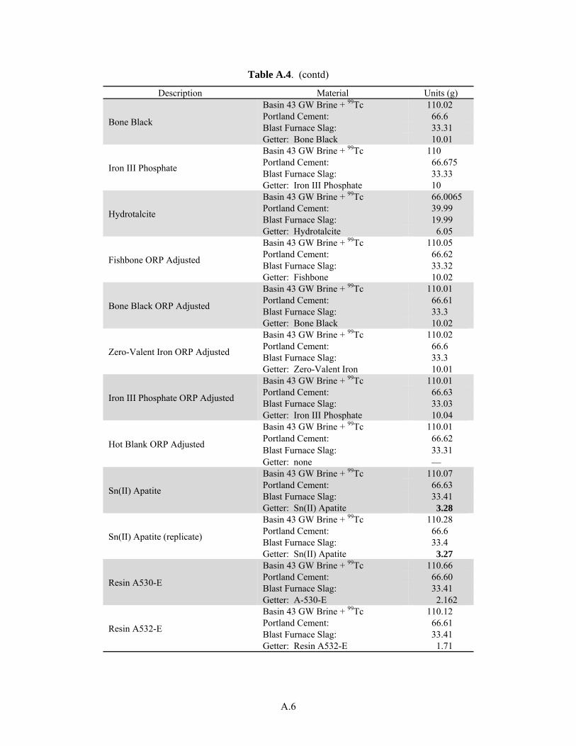
A.6

Table A.4. (contd)

Description Material Units (g)

Bone Black

Basin 43 GW Brine + 99Tc 110.02 Portland Cement: 66.6 Blast Furnace Slag: 33.31 Getter: Bone Black 10.01

Iron III Phosphate

Basin 43 GW Brine + 99Tc 110 Portland Cement: 66.675 Blast Furnace Slag: 33.33 Getter: Iron III Phosphate 10

Hydrotalcite

Basin 43 GW Brine + 99Tc 66.0065 Portland Cement: 39.99 Blast Furnace Slag: 19.99 Getter: Hydrotalcite 6.05

Fishbone ORP Adjusted

Basin 43 GW Brine + 99Tc 110.05 Portland Cement: 66.62 Blast Furnace Slag: 33.32 Getter: Fishbone 10.02

Bone Black ORP Adjusted

Basin 43 GW Brine + 99Tc 110.01 Portland Cement: 66.61 Blast Furnace Slag: 33.3 Getter: Bone Black 10.02

Zero-Valent Iron ORP Adjusted

Basin 43 GW Brine + 99Tc 110.02 Portland Cement: 66.6 Blast Furnace Slag: 33.3 Getter: Zero-Valent Iron 10.01

Iron III Phosphate ORP Adjusted

Basin 43 GW Brine + 99Tc 110.01 Portland Cement: 66.63 Blast Furnace Slag: 33.03 Getter: Iron III Phosphate 10.04

Hot Blank ORP Adjusted

Basin 43 GW Brine + 99Tc 110.01 Portland Cement: 66.62 Blast Furnace Slag: 33.31 Getter: none —

Sn(II) Apatite

Basin 43 GW Brine + 99Tc 110.07 Portland Cement: 66.63 Blast Furnace Slag: 33.41 Getter: Sn(II) Apatite 3.28

Sn(II) Apatite (replicate)

Basin 43 GW Brine + 99Tc 110.28 Portland Cement: 66.6 Blast Furnace Slag: 33.4 Getter: Sn(II) Apatite 3.27

Resin A530-E

Basin 43 GW Brine + 99Tc 110.66 Portland Cement: 66.60 Blast Furnace Slag: 33.41 Getter: A-530-E 2.162

Resin A532-E

Basin 43 GW Brine + 99Tc 110.12 Portland Cement: 66.61 Blast Furnace Slag: 33.41 Getter: Resin A532-E 1.71

A.7

The sorption tests using crushed waste forms were intended to simulate the case where rainwater infiltrates into the tank, dissolves 99Tc from the walls of the tank, and then contacts the cured stabilization grout that will be used to fill the empty tanks. The sorption tests (“clean” crushed Cast Stone contacting Tc-spiked solutions) were performed for 5 days and most of the Cast Stone mixes removed significant amounts (40 to 87% of Tc) from the DIW, and two tank supernate simulants. The Cast Stone mixes with BFS removed the most Tc from the solutions; likely via reduction/precipitation of the Tc. After the 5-day sorption test, the crushed Cast Stone containing “sorbed” Tc was leached for 20 days in DIW. The Cast Stone mixes with no BFS released all of the adsorbed Tc, but the Cast Stone mixes that contained BFS retained ~60% or the previously “adsorbed” Tc and released 40% back to the DIW.

For the long-term performance assessment of LAW forms in the IDF, the potential adsorption properties of the weathered/disaggregated waste forms should be considered. It appears that Cast Stone may be capable of adsorbing leached contaminants as well as being a source of leached contaminants.

A detailed campaign to study Tc getters was performed by Cooke et al. (2006, 2008), Guthrie et al. (2009), and Duncan et al. (2009), wherein a Basin 43 waste brine simulant (which represents contaminated Hanford groundwater concentrated by evaporation; see Table A.5,) was stabilized with a variant Cast Stone recipe that contained only Portland cement and the BFS at a 2:1 ratio. Pertechnetate, 92.17 mg L-1 Tc(VII), was added to the Basin 43 brine simulant, which resulted in a final waste-form concentration of 0.58 to 0.71 ppm 99Tc.

The two-component, Cast Stone dry blend was fortified by adding various Tc getters such that the final Cast Stone consisted of one part Basin 43 brine simulant to one part dry blend mix (consisting of the 2:1 Portland cement: BFS dry ingredients fortified with small masses of getters/reductants). The Tc getters studied are shown in Table A.6. The exact Basin 43 brine simulant and dry ingredient mixes are shown in Table A.7 (in Section A.4.2). Monoliths of this two-component Cast Stone variant (no fly ash is present) with Tc getters were cured at 54°C for 3 to 4 days, then at room temperature in their moisture-proof molds for the remaining time period to reach 28 days, and then ANS-16.1 leach tested for 5 days (the “abbreviated” leaching protocol).

Table A.5. Chemical composition of Basin brine simulant to test Tc getters.

Reagent g/L M Species M

NaNO3 140.7948 1.656 Na 2.143 MgSO4 19.6177 0.163 Mg 0.163 AlCl3 0.1337 0.001 Ca 0.146 KCl 2.7886 0.037 Ba 0.0001 BaCl2 0.0235 0.000 K 0.037 NaF 1.4126 0.034 Al 0.001 CaCl2 7.9349 0.071 NO3 1.656 Na2CrO4 0.1424 0.001 SO4 0.163 Ca(OH)2 5.5384 0.075 Cl 0.1834 Ca(NO3)2 42.3001 0.258 F 0.034 NaHCO3 37.8555 0.451 HCO3 0.451 Total Salts 258.5422 CrO4 0.001 OH 0.150

A.8

Table A.6. Tc getters and reductants used by Duncan et al. (2009) with Cast Stone waste-form variant.

Material Source

Getters Bone Black Ebonex PIMs (fish bone fines) UFA Ventures(e)

Reductants Ferrous sulfate 1 M Fisher Scientific(a) Iron powder (Fe°), ~325 mesh Fisher Scientific(a) Sodium metabisulfite Effluent Treatment Facility Tin(II) apatite Moore (2003)(b) Iron(III) phosphate Alfa Aesar(c)

Ion Exchange A530-E Purolite(d) A532-E Purolite(d) (a) Fisher Scientific is a trademark of the Fisher Scientific Company, Pittsburgh, Pennsylvania. (b) “Sorption of Tc by Sn(II) Treated Apatite Draft Letter Report, Sandia National Laboratories. (c) Alfa Aesar is a trademark of Johnson Matthey Public Limited Company, London, United

Kingdom. (d) Purolite is a trademark of the Brotech Corporation, Bala Cynwyd, Pennsylvania. (e) http://www.ufaventures.com/ufa_ventures/tech_briefs/apatite.html.

In general, 10 g (~3.3 g for Sn(II)-treated apatite and ~2 g for the Purolite® ion-exchange resins) of getter were added to the dry mix so that the final Brine 43 liquid-to-dry-blend-mix ratio became ~1 to 1 (110 g Brine 43, 66.6 g Portland cement, 33.3 g BFS, and 2 to 10 g Tc getter). For Cast Stone waste forms made with or without getters present (aside from the BFS), the Tc leach indices (LIs) after 5 days of leaching are shown in Figure A.1. The actual numerical data were not presented in tables in the cited references. From estimating the LI values from the figure and text in the citations, it can be concluded that the Tc LI for the Cast Stone variant with no getters was 11.25. As shown in Figure A.1, the getter Fishbone actually had a deleterious impact on the leachability of Tc, and the zero-valent iron reductant also had a slightly negative impact on the release of Tc from the Cast Stone variant monoliths. The hydrotalcite getter had no impact on Tc leachability, but all the other Tc getters/reductants improved the retention of Tc in the Cast Stone variant waste form. The Sn(II)- treated apatite and Purolite® anion exchange resins lowered the Tc release (diffusivity) by over a factor of 10 compared to the waste form with no Tc getters. The LI for the best getter, the Sn(II) treated apatite, was 12.7. The Cast Stone variant with 10 g of Sn(II) treated apatite in the dry blend had an effective diffusion coefficient of ~2 × 10-12 cm2 s-1. The overall ionic strength of the Brine 43 simulant is significantly lower than the LAW simulants used by Westsik et al. (2013) so the benefits of using Sn(II) treated apatite and the Purolite® anion exchange resins for the more saline LAW simulants will require further study. Note that the 7.8 M Na Ave simulant and Sn(II)- treated apatite have in fact been chosen for the lab testing reported in this report.

A.9

Figure A.1. Leachability indices for 99Tc from Cast Stone monoliths containing various getters (Duncan et al. 2009). Note in this figure, which is copied out of Duncan et al. (2009), that the amount of Sn(II) apatite used should be 2.78 g (not 1 g); also Purolite® A532-E is the correct description of the second resin.

The Duncan et al. (2009) Tc-getter studies using organic-based ion-exchange resins were effective in

the short tests but raise the concern that the Purolite® A 530-E and A 532-E might degrade and lose their anion retention properties over thousands of years. The stability of the organic-based anion exchange resins will need to be addressed if they are going to be considered as Tc getters.

A.4.1 Blast Furnace Slag – Tc Reductant (or Getter)

As mentioned, the Cast Stone dry blend used to date by Pacific Northwest National Laboratory (PNNL) to solidify and stabilize both LAW and secondary waste simulants and by Savannah River National Laboratory (SRNL) to solidify actual SRS tank wastes uses BFS in part to be an effective reductant for 99TcO4

- and possibly other redox-sensitive Resource Conservation and Recovery Act metals such as Cr(VI), Se(VI), and As(V). Slag was first studied as a reductant (as well as a key ingredient of grout dry blend) at SRNL. Most telling are leach test results discussed by Oblath (1984) and Langton (1988). Oblath created cementitious waste forms with a binary component dry blend of Class C fly ash and Class H cement (sulfate resistant and low heat of hydration) mixed with a simulated SRS tank salt brine solution. The mix was 40 wt% salt solution, 40% fly ash, and 20% cement. The simulated salt solution (32 wt% dissolved solids) was used after being spiked with tracer amounts of 95mTc, 85Sr, and 137Cs. The waste forms were 250-g samples (125 cm3 cylinders, geometric surface area 144 cm2). The waste forms were cured at either 18 days (open to air) or 28 days (in closed containers). The leach test was similar to the ANS-16.1 leach tests, but the DIW (500 mL) exchanges were performed at 1, 2, 3, 4, 5, 7,14, 21, 35, 42, 56, 63, 70, 77, 84, and 98 cumulative days. When cured in air, the surfaces dried out, and salt rind developed that leached into the first water contact. The samples cured in closed containers did not exhibit the “high blast” or wash-off of contaminants in the first leach solution. For this Saltstone variant, with no BFS, nitrate and technetium were equally leachable, cesium was released at 70%, and strontium was released at 4% of the nitrate release rate. The 99Tc leached at the same rate as the nitrate

A.10

because there was no BFS used in this Saltstone mix and apparently no reduction of the pertechnetate to the insoluble Tc(IV) species.

Langton (1988) shows significant differences in effective diffusion coefficients for Cr(VI) and 99Tc in variants of the Saltstone dry mix that includes BFS versus a mix without BFS for the same liquid waste simulant. When BFS is part of the dry mix at 25% of the final hardened Saltstone, the effective diffusion coefficients for Cr(VI) and 99Tc are 4 and almost 3 orders of magnitude lower than when BFS is not present in the waste form. Langton (1988) showed that the 99Tc LI for Saltstone increased from 8.3 to 11.4 (effective diffusion coefficient decreased from 5 10-9 to 3.9 10-12 cm2 s-1) when BFS was added to the dry blend in place of lime. Adding other 99Tc getters has not reduced 99Tc release much more than another order of magnitude beyond the leach rates controlled by the BFS, and aside from Purolite anion exchange resins, all the effective Tc getters currently known rely on their reduction capacity to lower the 99Tc leach properties. Thus, most 99Tc getters control 99Tc release in the same way as the BFS and may also lose their capacity to control the 99Tc release if oxygen overwhelms their reducing capacity.

Another study by Gilliam et al. (1990) solidified a filtrate liquid waste from “raffinate” from uranium recovery and equipment decontamination operations at the Portsmouth Gaseous Diffusion Plant in Portsmouth, Ohio. The acidic raffinate was diluted and the pH adjusted with sodium hydroxide to a value of 8.2 to 8.5. The pH adjustment resulted in the precipitation of metal hydroxides, which were further concentrated by filtration to yield a filter cake designated as heavy metals sludge (HMS) and an HMS filtrate. This liquid waste contains high amounts of sodium and nitrate (94 g L-1 [1.5 M]) and 13.7 mg L-1 99Tc. This HMS filtrate was solidified in a grout dry blend consisting of 1) Type I-II-LA Portland cement; 2) ASTM Class F fly ash from Centralia, Washington; and 3) granulated BFS. Four sources of BFS were evaluated:

material originating from Japan

material originating from Cleveland Republic Furnace No. 6

the Cleveland Republic Furnace No. 6 slag with gypsum added at 3 wt%

material from Sparrow’s Point, Maryland.

The grout had the following composition: 40 wt% HMS filtrate, 20-wt% BFS, 20-wt% ASTM Class F fly ash, and 20-wt% Type I-II-LA Portland cement. Each of the four BFSs was used in separate mixes. The resultant ANS-16.1 leach tests yielded LIs for 99Tc of 10.5 and for nitrate a value of 7.3. The source of the BFS does not measurably change the retention performance for technetium (LI = 10.5 ±0.5) or nitrate (LI = 7.3 ± 0.1). Gilliam et al.’s conclusion was that in the future, the source of BFS should be driven by economics rather than concerns about performance because any BFS seemed to lower 99Tc release similarly.

Gilliam et al. (1990) also investigated adding technical-grade sodium sulfide (Na2S•9H2O ~ 80% pure) to a grout dry-solids blend that consisted only of cement and fly ash. The added sodium sulfide significantly improved the retention of 99Tc as evidenced by the increase in 99Tc LI from 6.8 to 9.4. It can be hypothesized that porosity reduction and tortuosity increase in the grout matrix can be qualitatively observed by the LI for nitrate. Because nitrates are readily soluble in grout pore water, any significant improvement observed in its retention may be attributed to physical changes in porosity and tortuosity. The use of granulated BFS improved nitrate retention, but by a relatively small amount compared with

A.11

technetium. Thus, it can be concluded that the principal mechanism of improved Tc retention is a result of the reducing capacity of the BFS and not the resulting improved physical properties of the grout.

The obvious implication of Oblath’s (1984) and Langton’s (1988) studies, and many more recent ones, is that the BFS has reduced the Cr(VI) and Tc(VI) species to their much more insoluble Cr(III) and Tc(IV) species. To quantify the reducing capacity of BFS, as well as the other two ingredients cement and fly ash, Roberts and Kaplan (2009), Kaplan et al. (2008), Um et al. (2012, 2013), and Langton and Almond (2013) measured the reductive capacity of the dry blend ingredients used in Cast Stone and Saltstone. They found that the BFS has a large reductive capacity (~790 to 820 μeq g-1) compared to Portland cement (198 μeq g-1) and fly ash (299 μeq g-1). Regarding the general issue of oxidation state inside the final waste form, short-term measurements of the reduction capacity are problematic in that the measurements probably reflect a non-equilibrium situation in which good reducing agents, such as sulfur species within the BFS and stannous salts (used in other low-temperature waste-form recipes), coexist with oxidizing agents such as nitrate in the liquid wastes. Reductive capacity measurements on the freshly cured waste forms probably reflect the outcome of competing rapid reaction rates, but ultimately the relative masses of different reducing and oxidizing constituents, and the availability of oxygen in the final shallow land burial environment, will prevail over the long term. Predictive models will need to be used to assess how long it will take for the waste forms to reach redox equilibrium and at what oxidation-reduction potential (Eh) value the equilibrium is reached.

To corroborate that the significant decrease in leach properties of the redox-sensitive Tc element is in fact caused by reduction from the common oxidized form pertechnetate (TcO4

-) to some lower valence state, most likely the relatively stable Tc(IV) species; direct solid-phase analyses of the Tc speciation have been attempted. Allen et al. (1997), Shuh et al. (2010), Harbour and Aloy (2007), Lukens et al. (2005), and Um et al. (2011a,b, 2012, 2013) have directly determined the speciation of 99Tc in Saltstone and Cast Stone waste forms made with waste simulant using synchrotron X-ray absorption spectroscopy. Results have been somewhat variable dependent on the size of the Saltstone/Cast Stone specimen subjected to the synchrotron x-rays and the treatment of the Cast Stone specimens prior to being characterized (length of curing time, whether the specimen was leached or exposed to air prior to characterization and the conditions of leaching or air exposure). However, in all cases there has been definitive identification of reduced Tc(IV) within the cured and leached Saltstone/Cast Stone specimens along with identification of oxidized Tc(VII) pertechnetate likely present in the waste-form pore water. The reduced Tc(IV) is generally identified as discrete TcO2 particles or at lower percentages as Tc2S7, which has a structure where Tc(IV) is associated with polysulfide S2

2-. When there are ferrous-bearing iron minerals present some of the Tc(IV) has been shown to be associated with ferric oxy-hydroxides wherein the Tc(IV) atom replaces a Fe(III) ion in the ferric oxy-hydroxide crystal structure. This substitution is made possible because the two cations have a similar ionic radius. When the Tc(IV) is found within the Fe(III) oxyhydroxide crystal structure, it appears to be especially recalcitrant to re-oxidation to the more mobile Tc(VII) species (see Um et al. 2011b, 2012, 2013 and Kobayashi et al. 2013) for more discussion.

Regardless, the salient details from all these Tc speciation and release studies in grout are that 1) the BFS does reduce much of the pertechnetate anion from the +7 valence state to the +4 valence state and 2) the effective diffusion coefficient of 99Tc measured by standard monolith leach tests is thought to reflect oxygen diffusion into the cured grout, oxidation of the Tc(IV) by oxygen to Tc(VII), diffusion of the pertechnetate to the surface of the waste form, and release of pertechnetate to the solution.

A.12

A.4.2 Iodide Getters Used in Cast Stone Waste Forms

Layered bismuth hydroxides (LBHs), argentite (Ag2S), silver-impregnated carbon, and silver zeolites are identified in the literature as getters that have high affinity for I (Pierce et al. 2010). For example, the Kd values for iodide (I-) and iodate (IO3

-) varied between 631–25,119 and 50–39,811 mL g-1, respectively, in experiments conducted with layered Bi hydroxide (Krumhansl et al. 2006, cited by Pierce et al. 2010). In addition, Kd values of up to 80,000 mL g-1 were reported in experiments conducted using argentite and surface water with pH = 5.98 (Kaplan et al. 2000, cited by Pierce et al. 2010), and Kd values of 30,000 mL/g were reported in other experiments conducted using argentite and a glass leachate solution with varying pH (2.66 to 8.33) (Mattigod 2003). Finally, Kd values of 1,000 to 5,000 mL g-1 were reported in experiments conducted using Ag carbon and surface water with pH = 7.56 (Kaplan et al. 2000, cited by Pierce et al. 2010).

The results from another study conducted to estimate the effect of the solution-to-solid ratio on I sorption to argentite (Mattigod et al. 2003) demonstrated that sorption was the highest in experiments conducted with a low solution-to-solid ratio (about 100, or 0.1 g getter added in 10 mL of either groundwater or simulated glass leachate).

However, the sorption properties of both Tc and I getters vary considerably under different experimental conditions. For example, Moore (2003, cited by Mattigod et al. 2011b) reported Kd values between 475,000 and 3,202,100 mL g-1 for Tc sorption on Sn(II) treated apatite when groundwater with pH varying from 6 to 10 was used as the contacting solution. On the other hand, the Kd values were considerably smaller and varied within a narrower range (between 5,150–6,510 mL g-1) when a concentrated solution of NaNO3, NaNO2, and NaOH–NaAlO2 with pH = 13 was used as the background contacting solution in experiments conducted with the same material. This more saline and caustic solution is similar to LAW and secondary waste compositions and the 100-fold or larger decrease in Kd is noteworthy. This finding suggests finding efficient getters for Tc and I species in the LAW and secondary waste simulants could be challenging. There are fewer I getter studies than Tc-getter studies in the literature where the getters have been added to Cast Stone dry blend before mixing with waste simulants or actual waste.

Lockrem et al. (2005) added several getters to early Hanford Cast Stone dry blend formulations to solidify a Hanford Site secondary waste simulant (Table A.7) that contained high I concentrations spiked as NaI at starting concentrations of 4.25, 8.50, 17.0, 43.0, and 172 mg NaI L-1 of simulant. The secondary waste represents an iodine-rich caustic scrubber waste. The waste form itself represents solidifying a vitrification off-gas caustic scrubber waste stream. The sodium iodide was used as a surrogate for 129I that will be present in the actual waste. The level of sodium iodide (NaI) added was greater than the estimated activity of 129I in the actual waste stream by factors of about 7 to 280 in hopes of facilitating good analytical concentrations in the resultant leachates. In additional tests, Lockrem et al. (2005) used three concentrations (4.25, 8.50, and 17.0 mg/L as NaI) to observe the effect of increased waste-form iodide concentrations on the leachability of iodine from cured Cast Stone.

Iodide getters included two silver-bearing additives (silver zeolite and silver mordenite), two calcium phosphate compounds (Will Form; a calcium phosphate product designed to form a hydroxyapatite-like structure within the cement-based matrix), and bone char (Cosmic Black #7; a calcium phosphate animal bone charcoal product). The test matrix where these four getters were added to Cast Stone waste forms created with the secondary waste simulant spiked with various concentrations of iodide (and Hg(II)) are

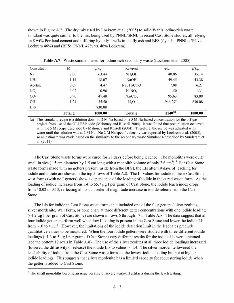
A.13

shown in Figure A.2. The dry mix used by Lockrem et al. (2005) to solidify this iodine-rich waste simulant was quite similar to the mix being used by PNNL/SRNL in recent Cast Stone studies, all relying on 8 wt% Portland cement and differing by only 1 wt% in the fly ash and BFS (fly ash: PNNL 45% vs. Lockrem 46%) and (BFS: PNNL 47% vs. 46% Lockrem).

Table A.7. Waste simulant used for iodine-rich secondary waste (Lockrem et al. 2005).

Constituent M g/kg Reagent g/L g/kg

Na 2.00 63.44 NH4OH 40.06 35.14

NH4 1.14 18.07 NaOH 49.45 43.38

Acetate 0.09 4.47 NaCH3COO 7.08 6.21

NO3 0.02 0.96 NaNO3 1.50 1.31

CO3 0.90 47.48 Na2CO3 95.63 83.88

OH 1.24 35.50 H2O 946.29(a) 830.08

H20 830.08

Total g 1000.00 Total g 1140(a) 1000.00

(a) This simulant recipe is a dilution down to 2 M Na based on a 5 M Na-based concentration for the off-gas project from use of the OLI-ESP code (Mahoney and Russell 2004). It was found that precipitation occurred with the 5 M recipe described by Mahoney and Russell (2004). Therefore, the recipe was adjusted with water until the solution was at 2 M Na. No 2 M Na specific density was reported by Lockrem et al. (2005), so an estimate was made based on the similarity to the secondary waste Simulant 4 described by Sundaram et al. (2011).

The Cast Stone waste forms were cured for 28 days before being leached. The monoliths were quite small in size (1.5 cm diameter by 1.5 cm long with a monolith volume of only 2.6 cm3).3 For Cast Stone waste forms made with no getters present (aside from the BFS), the LIs after 19 days of leaching for iodide and nitrate are shown in the top 5 rows of Table A.8. The LI values for iodide in these Cast Stone wast forms (with no I getters) show a dependence of the loading of iodide in the cured waste form. As the loading of iodide increases from 1.4 to 55.7 µg I per gram of Cast Stone, the iodide leach index drops from 10.02 to 9.13, reflecting almost an order of magnitude increase in iodide release from the Cast Stone.

The LIs for iodide in Cast Stone waste forms that included one of the four getters (silver zeolites, silver mordenite, Will Form, or bone char) at three different getter concentrations with one iodide loading (~1.2 µg I per gram of Cast Stone) are shown in rows 6 through 17 in Table A.8. The data suggest that all four iodide getters perform well when low I loading is present in the Cast Stone and lower the iodide LI from ~10 to >11.5. However, the limitations of the iodide detection limit in the leachates preclude quantitative values to be measured. When the four iodide getters were studied with three different iodide loadings (~1.3 to 5 µg I per gram of Cast Stone) very different results for the iodide LIs were obtained (see the bottom 12 rows in Table A.8). The use of the silver zeolites at all three iodide loadings increased (lowered the diffusivity or release) the iodide LIs to values >11.4. The silver mordenite lowered the leachability of iodide from the Cast Stone waste forms at the lowest iodide loading but not at higher iodide loadings. This suggests that silver mordenite has a limited capacity for sequestering iodide when the getter is added to Cast Stone. 3 The small monoliths become an issue because of severe wash-off artifacts during the leach testing.

A.14

Second waste simulant (spiked with I and Hg(II)) matrix for baseline Cast Stone waste forms (no getters present).

Second waste simulant (spiked with I and Hg(II)) matrix for silver zeolite getter testing.

Second waste simulant (spiked with I and Hg(II)) matrix for silver mordenite getter testing.

Figure A.2. Test matrix for studying iodide getters added to Cast Stone that solidified a Hanford secondary waste simulant.

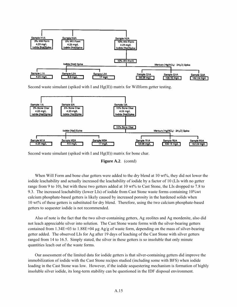
A.15

Second waste simulant (spiked with I and Hg(II)) matrix for Willform getter testing.

Second waste simulant (spiked with I and Hg(II)) matrix for bone char.

Figure A.2. (contd)

When Will Form and bone char getters were added to the dry blend at 10 wt%, they did not lower the

iodide leachability and actually increased the leachability of iodide by a factor of 10 (LIs with no getter range from 9 to 10), but with these two getters added at 10 wt% to Cast Stone, the LIs dropped to 7.8 to 9.3. The increased leachability (lower LIs) of iodide from Cast Stone waste forms containing 10%wt calcium phosphate-based getters is likely caused by increased porosity in the hardened solids when 10 wt% of these getters is substituted for dry blend. Therefore, using the two calcium phosphate-based getters to sequester iodide is not recommended.

Also of note is the fact that the two silver-containing getters, Ag zeolites and Ag mordenite, also did not leach appreciable silver into solution. The Cast Stone waste forms with the silver-bearing getters contained from 1.34E+03 to 1.88E+04 µg Ag/g of waste form, depending on the mass of silver-bearing getter added. The observed LIs for Ag after 19 days of leaching of the Cast Stone with silver getters ranged from 14 to 16.5. Simply stated, the silver in these getters is so insoluble that only minute quantities leach out of the waste forms.

Our assessment of the limited data for iodide getters is that silver-containing getters did improve the immobilization of iodide with the Cast Stone recipes studied (including some with BFS) when iodide loading in the Cast Stone was low. However, if the iodide sequestering mechanism is formation of highly insoluble silver iodide, its long-term stability can be questioned in the IDF disposal environment.

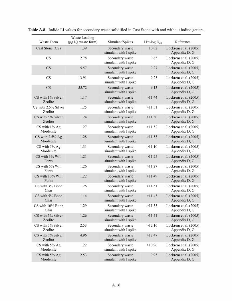
A.16

Table A.8. Iodide LI values for secondary waste solidified in Cast Stone with and without iodine getters.

Waste Form Waste Loading

(μg I/g waste form) Simulant/Spikes LI=-log Deff Reference

Cast Stone (CS) 1.39 Secondary waste simulant with I spike

10.02 Lockrem et al. (2005) Appendix D, G

CS 2.78 Secondary waste simulant with I spike








CS with 1% Silver Zeolite

1.17 Secondary waste simulant with I spike

>11.44 Lockrem et al. (2005) Appendix D, G

CS with 2.5% Silver Zeolite






CS with 1% Ag Mordenite



CS with 2.5% Ag Mordenite






CS with 3% Will Form









CS with 3% Bone Char
























A.17

Table A.8. (contd)

Waste Form Waste Loading

(μg I/g waste form) Simulant/Spikes LI=-log Deff Reference






















Note: All leach tests were 19-day long ANS16.1 tests.

The following analysis of silver iodide stability was provided by Dr. Jim Krumhansl (recently retired from Sandia National Laboratory) as part of his review of the draft version of Serne and Westsik (2011). The AgI solubility is lowest at intermediate fugacities of oxygen that lie between conditions likely to be encountered at the Earth’s surface and those likely to be established during the corrosion of various metallic waste package materials, as shown in Figure A.2. At the Earth’s surface the calculations indicate that AgI is transformed to the much more soluble AgIO3, while under strongly reducing conditions AgI releases iodide as it breaks down to form silver metal.

Although not expected in the IDF disposal environment, bacterial reduction of sulfate can produce iron pyrite (FeS2) or H2S, both of which promote formation of Ag2S. This bacterial reduction process is an additional pathway for destabilizing AgI. It should be noted that none of these reactions occurs rapidly enough to be easily observed in the short-term lab waste-form leaching studies performed to date. Hence, short-term studies will generally just reflect the extremely low solubility of AgI. Note also that the high iodine concentrations at the extremities of Figure A.3 are the result of the amount of AgI added to the model, and do not indicate some sort of a solubility limit. Table A.9 shows the fugacity of several common redox couples germane to subsurface environments.

The lower curve in Figure A.3 represents iodine concentrations in equilibrium with a mix of AgI and AgCl, while the upper curve represents the solubility of just AgI. The difference can be ascribed to the common ion effect and the fact that AgCl is somewhat more soluble than AgI so the presence of AgCl elevates the dissolved Ag+ concentration, thereby suppressing the dissolved iodide (or at high-oxygen fugacity iodate) concentration.

Another observation provided by reviewer Dr. Krumhansl is that one should be able to improve the effectiveness of any getter by mixing the getter and waste fluid together (and letting the mix sit for some time) prior to adding the principal Cast Stone dry blend components, because once the target

A.18

contaminants are firmly fixed to the getter it is less likely that the other chemical reactions that occur when the Cast Stone sets will be able to dislodge them.

Figure A.3. AgI solubility at 25°C and in a pH 7 solution as a function of oxygen fugacity. Lower

curve (pink) represents iodine concentrations in equilibrium with a mix of AgI and AgCl while the upper curve (blue) represents solubility of just AgI.

Table A.9. Reference oxygen fugacities for useful buffer systems.

Oxygen Buffer Oxygen Fugacity (at pH 7)

Earth’s surface 0.2 (10-0.698)

AgIO3 - AgI 10-3.17

Ag metal - AgI 10-40.62

Schoepite [UO2(OH)2H2O] - Uraninite (UO2) 10-44.7

Cu-Cu2O 10-51.9

Magnetite [Fe3O4] - Hematite [Fe2O3] 10-72.3

Pb - PbO 10-75.4

Fugacities were calculated using the REACT code <http://chemicalsoft.com/> using thermodynamic data from Wagman et al. (1982). More details are available from Dr. Jim Krumhansl, retired from Sandia National Laboratory, [email protected].

A.5 Wash-Off Phenomenon in Cast Stone in Laboratory Leach Tests

Incremental effective diffusivity coefficients for Cast Stone (or any cementitious waste form) tests for leach intervals generally decrease by at least 2 orders of magnitude for Tc and by 1 order of magnitude for Na and iodide in typical ANS16.1 or EPA Method 1315 intermittent solution exchange leach tests.

AgI solubility

-2

-1

0

1

2

3

4

5

-70 -60 -50 -40 -30 -20 -10 0

Log[ Oxygen Fugacity ]

Lo

g[

pp

m i

od

ine

]

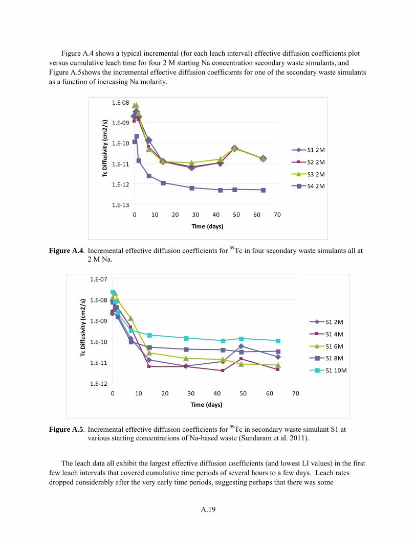
A.19

Figure A.4 shows a typical incremental (for each leach interval) effective diffusion coefficients plot versus cumulative leach time for four 2 M starting Na concentration secondary waste simulants, and Figure A.5shows the incremental effective diffusion coefficients for one of the secondary waste simulants as a function of increasing Na molarity.

Figure A.4. Incremental effective diffusion coefficients for 99Tc in four secondary waste simulants all at 2 M Na.

Figure A.5. Incremental effective diffusion coefficients for 99Tc in secondary waste simulant S1 at various starting concentrations of Na-based waste (Sundaram et al. 2011).

The leach data all exhibit the largest effective diffusion coefficients (and lowest LI values) in the first

few leach intervals that covered cumulative time periods of several hours to a few days. Leach rates dropped considerably after the very early time periods, suggesting perhaps that there was some

1.E‐13

1.E‐12

1.E‐11

1.E‐10

1.E‐09

1.E‐08

0 10 20 30 40 50 60 70

Time (days)

Tc Diffusivity (cm

2/s)

S1 2M

S2 2M

S3 2M

S4 2M

1.E‐12

1.E‐11

1.E‐10

1.E‐09

1.E‐08

1.E‐07

0 10 20 30 40 50 60 70

Time (days)

Tc Diffusivity (cm

2/s)

S1 2M

S1 4M

S1 6M

S1 8M

S1 10M

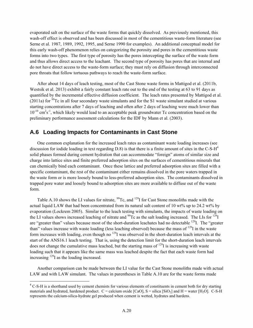
A.20

evaporated salt on the surface of the waste forms that quickly dissolved. As previously mentioned, this wash-off effect is observed and has been discussed in most of the cementitious waste-form literature (see Serne et al. 1987, 1989, 1992, 1995, and Serne 1990 for examples). An additional conceptual model for this early wash-off phenomenon relies on categorizing the porosity and pores in the cementitious waste forms into two types. The first type of porosity has the pores intercepting the surface of the waste form and thus allows direct access to the leachant. The second type of porosity has pores that are internal and do not have direct access to the waste-form surface; they must rely on diffusion through interconnected pore throats that follow tortuous pathways to reach the waste-form surface.

After about 14 days of leach testing, most of the Cast Stone waste forms in Mattigod et al. (2011b, Westsik et al. 2013) exhibit a fairly constant leach rate out to the end of the testing at 63 to 91 days as quantified by the incremental effective diffusion coefficient. The leach rates presented by Mattigod et al. (2011a) for 99Tc in all four secondary waste simulants and for the S1 waste simulant studied at various starting concentrations after 7 days of leaching and often after 2 days of leaching were much lower than 10-10 cm2s-1, which likely would lead to an acceptable peak groundwater Tc concentration based on the preliminary performance assessment calculations for the IDF by Mann et al. (2003).

A.6 Loading Impacts for Contaminants in Cast Stone

One common explanation for the increased leach rates as contaminant waste loading increases (see discussion for iodide loading in text regarding D.8) is that there is a finite amount of sites in the C-S-H4 solid phases formed during cement hydration that can accommodate “foreign” atoms of similar size and charge into lattice sites and finite preferred adsorption sites on the surfaces of cementitious minerals that can chemically bind each contaminant. Once these lattice and preferred adsorption sites are filled with a specific contaminant, the rest of the contaminant either remains dissolved in the pore waters trapped in the waste form or is more loosely bound to less-preferred adsorption sites. The contaminants dissolved in trapped pore water and loosely bound to adsorption sites are more available to diffuse out of the waste form.

Table A.10 shows the LI values for nitrate, 99Tc, and 129I for Cast Stone monoliths made with the actual liquid LAW that had been concentrated from its natural salt content of 10 wt% up to 24.2 wt% by evaporation (Lockrem 2005). Similar to the leach testing with simulants, the impacts of waste loading on the LI values shows increased leaching of nitrate and 99Tc as the salt loading increased. The LIs for 129I are “greater than” values because most of the short-duration leachates had no detectable 129I. The “greater than” values increase with waste loading (less leaching observed) because the mass of 129I in the waste form increases with loading, even though no 129I was observed in the short-duration leach intervals at the start of the ANS16.1 leach testing. That is, using the detection limit for the short-duration leach intervals does not change the cumulative mass leached, but the starting mass of 129I is increasing with waste loading such that it appears like the same mass was leached despite the fact that each waste form had increasing 129I as the loading increased.

Another comparison can be made between the LI value for the Cast Stone monoliths made with actual LAW and with LAW simulant. The values in parentheses in Table A.10 are for the waste forms made

4 C-S-H is a shorthand used by cement chemists for various elements of constituents in cement both for dry starting materials and hydrated, hardened product. C = calcium oxide [CaO], S = silica [SiO2] and H = water [H2O]. C-S-H represents the calcium-silica-hydrate gel produced when cement is wetted, hydrates and hardens.

A.21

with simulant at the same total salt loadings as those used in Cast Stone made with the actual LAW. It appears that slightly less nitrate leaches from waste forms made with actual waste than from waste forms made with LAW simulant at the same total salt loadings. However, the differences are likely not significant.

Thus loading impacts (both for the waste composition and for the amount of getters substituted for Cast Stone dry blend) need to be carefully considered when interpreting the release of contaminants from Cast Stone waste forms. All of the issues identified in this literature review are being considered in the getter testing that is under way and discussed in the following sections.

Table A.10. LI values for nitrate, 99Tc, and 129I for Cast Stone monoliths made with actual LAW.

Waste Loading wt%

LI (47 days)

Nitrate 99Tc 129I

10.2 8.5, (8.3) 10.4 >7.9

16.1 7.8, (7.6) 10 >8.3

18.8 7.7, (7.67) 9.8 >8.6

18.8 7.5 9.8 >8.5

19.2 7.5 9.8 >8.6

21.8 7.6, (7.1) 9.7 >8.7

24.2 7.5, (7.2) 9.5 >8.8

Values in parentheses are for the Cast Stone waste forms made with LAW simulant.

Appendix B –

X-ray Diffraction Spectra for the Getters Used in this Study

B

.3

SnCl2 ground

00-054-2050 (N) - Tris(1-decyloxy-2,2`,3,3`,4`,6,6`-heptadecanoyl cellobiose)-1,3,5-benzenetrica - C285H504O60 - Y: 3.35 % - a 43.10000 - b 35.50000 - c 5.41000 - alpha 90.000 - beta 90.000 - gamma 10

01-072-0137 (I) - Tin Chloride - SnCl2 - Y: 60.30 % - a 7.79300 - b 9.20700 - c 4.43000 - alpha 90.000 - beta 90.000 - gamma 90.000 - Primitive - Pnam (62) - I/Ic PDF 3.3

Operations: Strip kAlpha2 0.500 | Background 0.120,1.000 | Import

SnCl2 ground - File: SnCl2 ground.raw - Type: Locked Coupled - Start: 5.000 ° - End: 79.342 ° - Step: 0.015 ° - Step time: 53.1 s - Temp.: 25 °C (Room) - Time Started: 16 s - 2-Theta: 5.000 ° - Theta: 2.500

Lin

(Cou

nts)

0

1000

2000

3000

4000

5000

6000

7000

8000

9000

10000

2-Theta - Scale

6 10 20 30 40 50 60 70

B

.4

Silver-impregnated carbon

020

000

4000

060

000

Cou

nts

10 20 30 40 50 60 70 80 90

2Theta (Coupled TwoTheta/Theta) WL=1.54060

B

.5

Ag zeolite

010

000

2000

030

000

4000

050

000

Cou

nts

10 20 30 40 50 60 70 80 90


010

000

2000

030

000

4000

050

000

Cou

nts

10 20 30 40 50 60 70 80 90


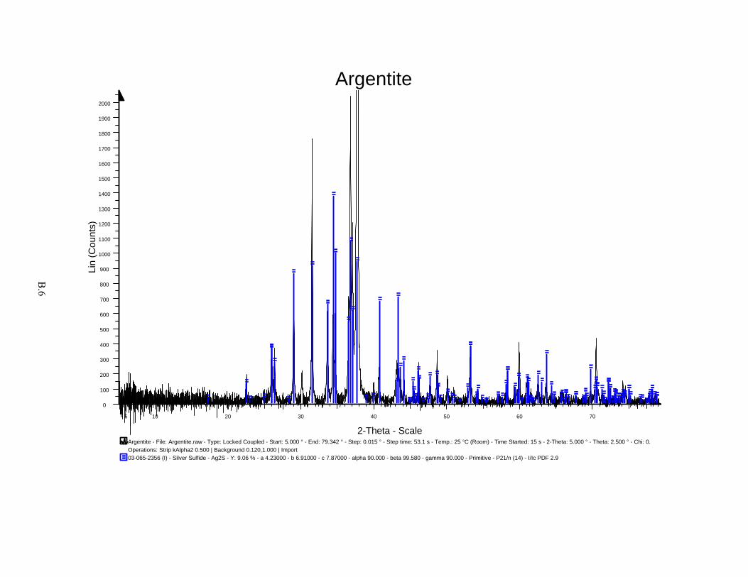
B

.6

Argentite

03-065-2356 (I) - Silver Sulfide - Ag2S - Y: 9.06 % - a 4.23000 - b 6.91000 - c 7.87000 - alpha 90.000 - beta 99.580 - gamma 90.000 - Primitive - P21/n (14) - I/Ic PDF 2.9


Argentite - File: Argentite.raw - Type: Locked Coupled - Start: 5.000 ° - End: 79.342 ° - Step: 0.015 ° - Step time: 53.1 s - Temp.: 25 °C (Room) - Time Started: 15 s - 2-Theta: 5.000 ° - Theta: 2.500 ° - Chi: 0.

Lin

(Cou

nts)

0

100

200

300

400

500

600

700

800

900

1000

1100

1200

1300

1400

1500

1600

1700

1800

1900

2000

2-Theta - Scale

6 10 20 30 40 50 60 70

B

.7

Synthetic Argentite

03-065-2356 (I) - Silver Sulfide - Ag2S - Y: 9.06 % - a 4.23000 - b 6.91000 - c 7.87000 - alpha 90.000 - beta 99.580 - gamma 90.000 - Primitive - P21/n (14) - I/Ic PDF 2.9


Synthetic Argentite - File: Synthetic Argentite.raw - Type: Locked Coupled - Start: 5.000 ° - End: 79.342 ° - Step: 0.015 ° - Step time: 53.1 s - Temp.: 25 °C (Room) - Time Started: 15 s - 2-Theta: 5.000 ° - Th

Lin

(Cou

nts)

0

100

200

300

400

500

600

700

800

900

1000

1100

1200

1300

1400

1500

1600

1700

1800

1900

2000

2-Theta - Scale

6 10 20 30 40 50 60 70

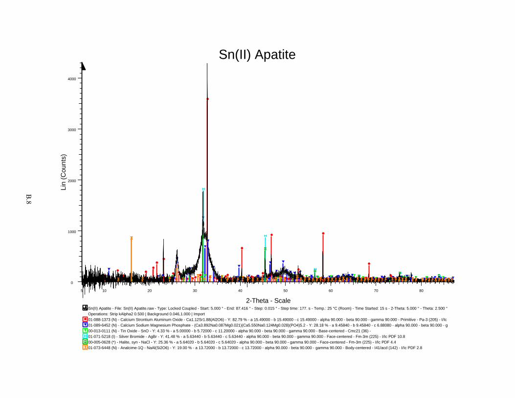
B

.8

Sn(II) Apatite

01-073-6448 (N) - Analcime-1Q - NaAl(Si2O6) - Y: 19.00 % - a 13.72000 - b 13.72000 - c 13.72000 - alpha 90.000 - beta 90.000 - gamma 90.000 - Body-centered - I41/acd (142) - I/Ic PDF 2.8

00-005-0628 (*) - Halite, syn - NaCl - Y: 25.36 % - a 5.64020 - b 5.64020 - c 5.64020 - alpha 90.000 - beta 90.000 - gamma 90.000 - Face-centered - Fm-3m (225) - I/Ic PDF 4.4

01-071-5218 (I) - Silver Bromide - AgBr - Y: 41.48 % - a 5.63440 - b 5.63440 - c 5.63440 - alpha 90.000 - beta 90.000 - gamma 90.000 - Face-centered - Fm-3m (225) - I/Ic PDF 10.8

00-013-0111 (N) - Tin Oxide - SnO - Y: 4.33 % - a 5.00000 - b 5.72000 - c 11.20000 - alpha 90.000 - beta 90.000 - gamma 90.000 - Base-centered - Cmc21 (36) -

01-089-6452 (N) - Calcium Sodium Magnesium Phosphate - (Ca3.892Na0.087Mg0.021)(Ca5.550Na0.124Mg0.028)(PO4)5.2 - Y: 28.18 % - a 9.45840 - b 9.45840 - c 6.88080 - alpha 90.000 - beta 90.000 - g

01-088-1373 (N) - Calcium Strontium Aluminum Oxide - Ca1.12Sr1.88(Al2O6) - Y: 82.79 % - a 15.49000 - b 15.49000 - c 15.49000 - alpha 90.000 - beta 90.000 - gamma 90.000 - Primitive - Pa-3 (205) - I/Ic


Sn(II) Apatite - File: Sn(II) Apatite.raw - Type: Locked Coupled - Start: 5.000 ° - End: 87.416 ° - Step: 0.015 ° - Step time: 177. s - Temp.: 25 °C (Room) - Time Started: 15 s - 2-Theta: 5.000 ° - Theta: 2.500 °

Lin

(Cou

nts

)

0

1000

2000

3000

4000

2-Theta - Scale

5 10 20 30 40 50 60 70 80

B

.9

Tin hydroxyapatite

010

0020

0030

0040

0050

0060

00

Cou

nts

10 20 30 40 50 60 70 80 90


040

0080

0012

000

1600

0

Cou

nts

10 20 30 40 50 60 70 80 90


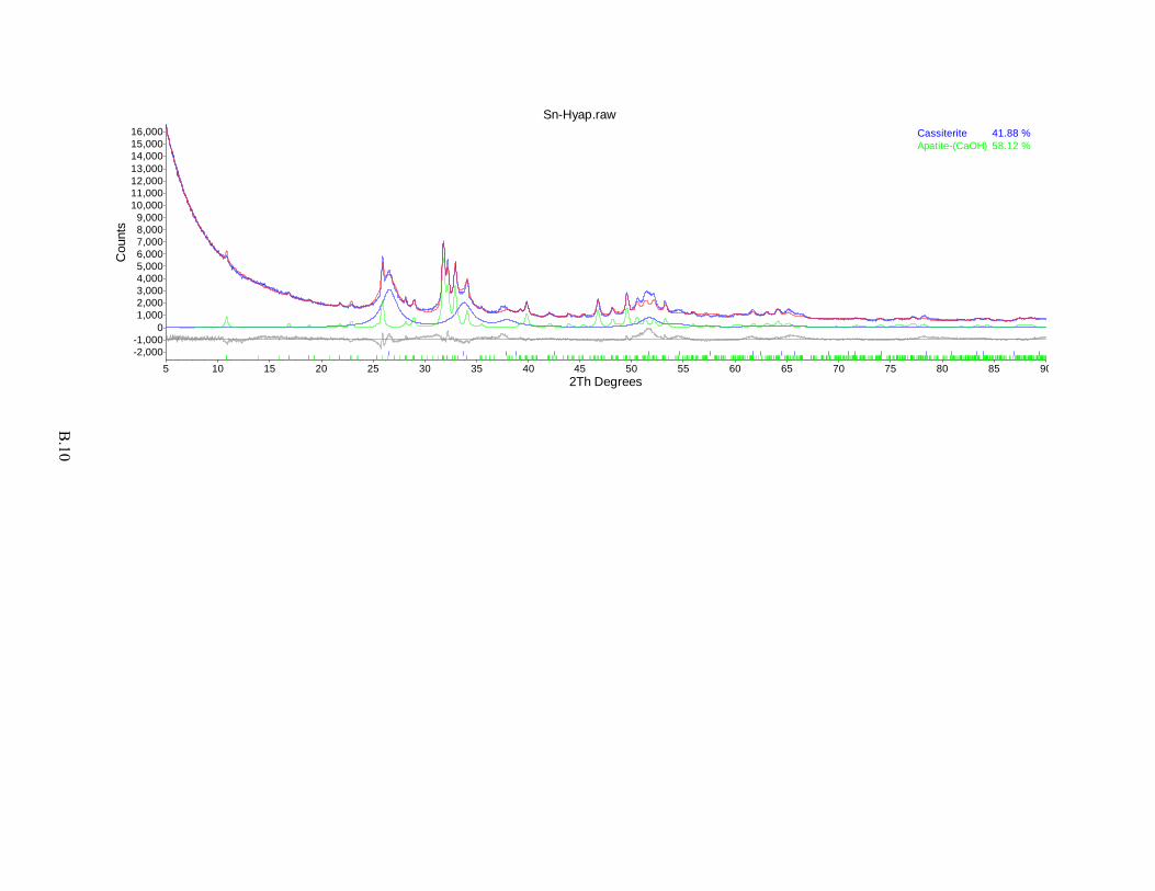
B

.10

Sn-Hyap.raw

2Th Degrees90858075706560555045403530252015105

Cou

nts

16,00015,00014,00013,00012,00011,00010,000

9,0008,0007,0006,0005,0004,0003,0002,0001,000

0-1,000-2,000

Cassiterite 41.88 %Apatite-(CaOH) 58.12 %

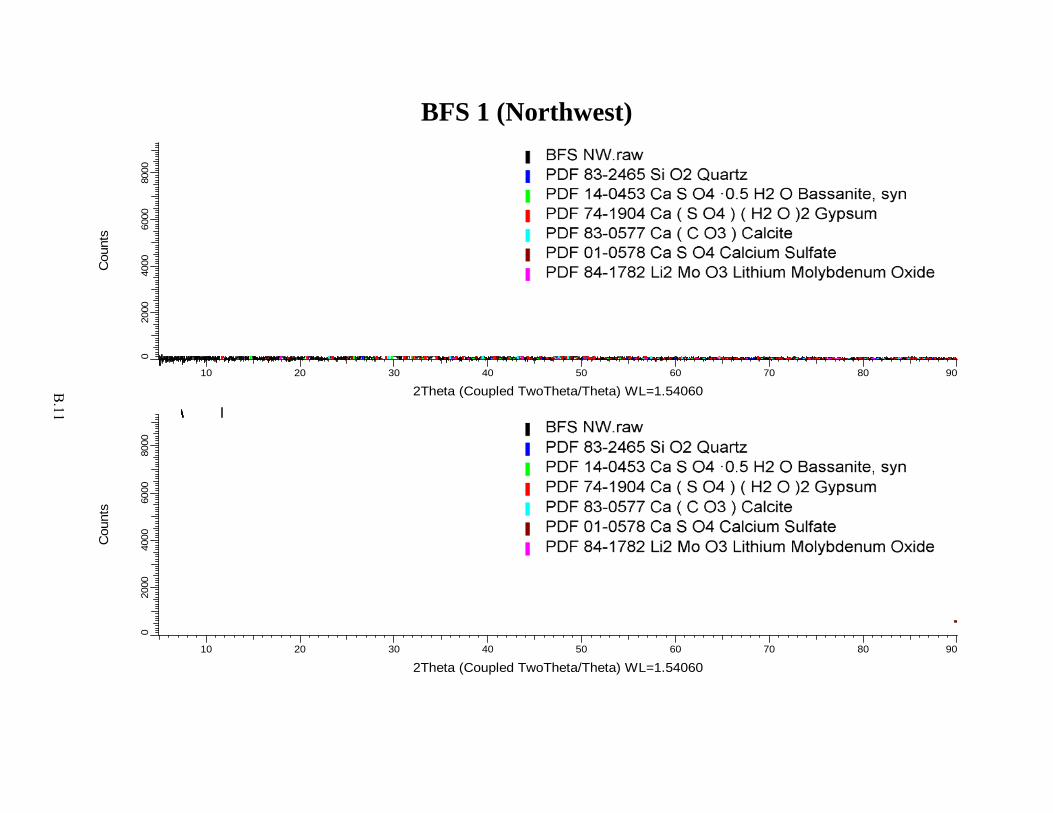
B

.11

BFS 1 (Northwest)

159

131

020

0040

0060

0080

00

Cou

nts

10 20 30 40 50 60 70 80 90


159

131

020

0040

00

6000

8000

Cou

nts

10 20 30 40 50 60 70 80 90


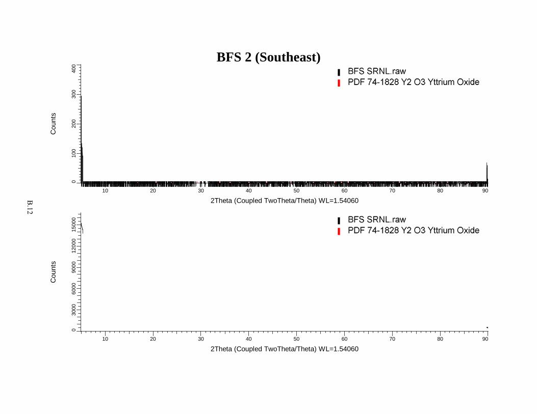
B

.12

BFS 2 (Southeast)

010

020

030

040

0

Cou

nts

10 20 30 40 50 60 70 80 90


030

0060

0090

0012

000

1500

0

Cou

nts

10 20 30 40 50 60 70 80 90


B

.13

Layered Bismuth Hydroxide

LBU Attempt A.raw_1

2Th Degrees75706560555045403530252015105

Co

un

ts

15,000

14,000

13,000

12,000

11,000

10,000

9,000

8,000

7,000

6,000

5,000

4,000

3,000

2,000

1,000

0

-1,000

-2,000

P4 0.00 %

B

.14

KMS

KMS.raw

2Th Degrees605856545250484644424038363432302826242220181614121086

Co

un

ts

52,000

50,000

48,000

46,000

44,000

42,000

40,000

38,000

36,000

34,000

32,000

30,000

28,000

26,000

24,000

22,000

20,000

18,000

16,000

14,000

12,000

10,000

8,000

6,000

4,000

2,000

0

-2,000

-4,000

-6,000

-8,000

I4132 0.00 %Magnesite 100.00 %

B

.15

Nano SNP

00-035-0769 (*) - Cyanochroite, syn - K2Cu+2(SO4)2·6H2O - Y: 4.77 % - a 9.08000 - b 12.12300 - c 6.16400 - alpha 90.000 - beta 104.441 - gamma 90.000 - Primitive - P21/a (14) -

00-058-1236 (*) - N-(4-(Diethylamino)benzylidene)-4-phenyl-5-(1,2,4-triazol-1-yl)thiazol-2-amine - C22H22N6S - Y: 2.33 % - a 9.05835 - b 20.92756 - c 11.49940 - alpha 90.000 - beta 108.644 - gamma 90.0

00-035-0028 (Q) - Tin Phosphate - Sn2P2O7 - Y: 13.84 % -

01-072-7509 (I) - Rutile - Sn0.9(O1.6(OH)0.4) - Y: 22.07 % - a 4.73300 - b 4.73300 - c 3.18340 - alpha 90.000 - beta 90.000 - gamma 90.000 - Primitive - P42/mnm (136) - I/Ic PDF 8.5


Nano SNP - File: Nano SNP.raw - Type: Locked Coupled - Start: 5.000 ° - End: 79.342 ° - Step: 0.015 ° - Step time: 53.1 s - Temp.: 25 °C (Room) - Time Started: 14 s - 2-Theta: 5.000 ° - Theta: 2.500 ° - Chi

Lin

(Cou

nts)

0

1000

2000

3000

4000

2-Theta - Scale

6 10 20 30 40 50 60 70

Appendix C –

Effluent Concentrations, pH Values, and Calculated Kd Values

C.1

Appendix C

Effluent Concentrations, Calculated Kd Values, and pH values

Batch effluent concentrations and calculated Kd values (mL/g for the deionized water and 7.8 M LAW simulant samples are contained in Tables C.1 through C.6. Tables C.7 through C.10 include the pH measured after 10 to 14 days of contact. The “blank set” name in the latter tables shows which blank samples were run with a given sample set.

C

.2

Table C.1.

Sample ID Sample time (days) Vol. solution, mL

DDI Samples

[Tc], A (µg/L)

[Tc], B (µg/L)

log(average Kd),

[mL/g]

stdev log(average

Kd)

log[(average Kd)/SA], [m × 10-6]

log[(stdev Kd)/SA], [m × 10-6] Notes

BFS 1-C1-1 0.2 100 5.38E+03 5.50E+03 0 --- --- ---

BFS 1-C1-2 0.9 98 5.09E+03 5.48E+03 0 --- --- ---

BFS 1-C1-3 3.0 96 3.44E+03 3.85E+03 1.68 0.99 1.40 0.72

BFS 1-C1-4 6.0 94 2.62E+03 3.03E+03 1.84 1.16 1.56 0.88

BFS 1-C1-5 10.0 92 1.96E+03 2.45E+03 2.08 1.47 1.80 1.19

BFS 1-C1-6 14.0 90 1.53E+03 1.65E+03 2.29 0.92 2.01 0.64

BFS 1-C1-7 16.9 88 1.38E+03 9.94E+02 2.46 1.98 2.18 1.70

BFS 1-C1-8 35.0 86 2.05E+01 2.05E+01 4.35 2.90 4.07 3 used EQL

BFS 1-C2-1 0.2 100 2.79E+04 2.78E+04 0 --- --- ---

BFS 1-C2-2 0.9 98 2.72E+04 2.72E+04 0 --- --- ---

BFS 1-C2-3 3.0 96 2.71E+04 2.76E+04 0.51 0.12 0.24 -0.16

BFS 1-C2-4 6.0 94 2.37E+04 2.30E+04 1.14 0.37 0.86 0.09

BFS 1-C2-5 10.0 92 2.23E+04 2.26E+04 1.30 0.04 1.02 -0.24

BFS 1-C2-6 14.0 90 2.11E+04 2.26E+04 1.35 0.75 1.07 0.47

BFS 1-C2-7 16.9 88 1.94E+04 2.06E+04 1.46 0.71 1.18 0.43

BFS 1-C2-8 35.0 86 2.05E+02 1.84E+04 3.76 3.91 3.48 3.63 used EQL

BFS 1-C3-1 0.2 100 5.31E+04 5.74E+04 -1.01 --- -1.30 ---

BFS 1-C3-2 1.0 98 5.56E+04 5.57E+04 0 --- --- ---

BFS 1-C3-3 3.0 96 5.57E+04 5.53E+04 0 --- --- ---

BFS 1-C3-4 6.0 94 5.03E+04 4.93E+04 0.74 0.16 0.46 -0.12

BFS 1-C3-5 10.0 92 4.69E+04 4.87E+04 1.02 0.45 0.74 0.17

BFS 1-C3-6 14.0 90 4.61E+04 4.71E+04 1.10 0.20 0.82 -0.07

BFS 1-C3-7 17.0 88 4.46E+04 4.60E+04 1.15 0.36 0.87 0.08

BFS 1-C3-8 35.0 86 1.78E+04 1.94E+04 2.22 1.19 1.94 0.91

C

.3

Table C.1. (contd)


DDI Samples

[Tc], A (µg/L)

[Tc], B (µg/L)

log(average Kd), [mL/g]

stdev log(average

Kd) log(Kd/SA),

[m × 10-6]

log[(average Kd)/SA], [m × 10-6] Notes

BFS 2-C1-1 0.2 100 3.88E+03 4.23E+03 1.35 0.90 1.03 0.57

BFS 2-C1-2 0.9 98 3.59E+03 4.07E+03 1.48 1.08 1.16 0.75

BFS 2-C1-3 3.0 96 2.91E+03 2.67E+03 1.95 0.97 1.63 0.65

BFS 2-C1-4 6.0 94 5.04E+02 1.20E+03 2.74 2.58 2.42 2.26

BFS 2-C1-5 10.0 92 5.47E+01 1.11E+02 3.79 3.49 3.47 3.17

BFS 2-C1-6 14.0 90 3.85E+00 4.66E+00 5.02 4.21 4.70 3.89

BFS 2-C1-7 16.9 88 1.41E+00 9.35E-01 5.57 5.00 5.25 4.68

BFS 2-C1-8 35.0 86 8.20E-02 8.20E-02 6.73 5.05 6.41 4.73 used EQL

BFS 2-C2-1 0.2 100 2.57E+04 2.60E+04 0.29 -0.04 -0.04 -0.36

BFS 2-C2-2 0.9 98 2.56E+04 2.53E+04 0.77 -0.25 0.45 -0.57

BFS 2-C2-3 3.0 96 2.41E+04 2.35E+04 1.25 0.06 0.93 -0.26

BFS 2-C2-4 6.0 94 2.02E+04 1.78E+04 1.58 0.99 1.26 0.67

BFS 2-C2-5 10.0 92 1.63E+04 1.33E+04 1.89 1.31 1.57 0.99

BFS 2-C2-6 14.0 90 1.06E+04 6.38E+03 2.32 1.98 2.00 1.66

BFS 2-C2-7 16.9 88 4.50E+03 6.46E+02 3.28 3.31 2.95 2.99

BFS 2-C2-8 35.0 86 2.05E+01 2.05E+01 5.04 3.73 4.72 3.41 used EQL

BFS 2-C3-1 0.2 100 5.22E+04 5.29E+04 0.06 -0.01 -0.26 -0.33

BFS 2-C3-2 0.9 98 5.30E+04 5.32E+04 0.56 -0.45 0.23 -0.77

BFS 2-C3-3 3.0 96 5.08E+04 5.28E+04 0.66 0.48 0.34 0.15

BFS 2-C3-4 6.0 94 4.44E+04 4.41E+04 1.29 -0.75 0.97 -1.08

BFS 2-C3-5 10.0 92 4.12E+04 4.06E+04 1.49 -0.13 1.16 -0.45

BFS 2-C3-6 14.0 90 3.41E+04 3.26E+04 1.79 0.60 1.47 0.28

BFS 2-C3-7 16.9 88 2.74E+04 2.36E+04 2.05 1.31 1.73 0.99

BFS 2-C3-8 35.0 86 2.05E+02 2.05E+02 4.44 2.77 4.12 2.44 used EQL

C

.4

Table C.1. (contd)


DDI Samples

[Tc], A (µg/L)

[Tc], B (µg/L)


stdev log(average

Kd) log(Kd/SA),

[m × 10-6]


Tin Apatite-C1-1 0.2 100 1.18E+03 1.25E+03 2.97 1.70 0.95 -0.32

Tin Apatite-C1-2 0.9 98 4.29E+02 5.64E+02 3.44 2.77 1.42 0.75

Tin Apatite-C1-3 3.0 96 2.61E+00 3.32E+00 5.73 4.96 3.71 2.94

Tin Apatite-C1-4 6.0 94 5.03E-01 3.13E+00 6.21 6.22 4.19 4.20

Tin Apatite-C1-5 10.0 92 5.61E-01 4.26E-01 6.46 5.75 4.44 3.73

Tin Apatite-C1-6 14.0 90 2.20E+00 7.49E-01 6.08 5.93 4.06 3.91

Tin Apatite-C1-7 16.9 88 3.10E-01 3.51E-01 6.60 5.54 4.57 3.52

Tin Apatite-C1-8 35.0 86 1.48E-01 2.12E-01 6.89 6.30 4.87 4.27

Tin Apatite-C2-1 0.2 100 1.03E+04 9.96E+03 2.69 1.18 0.67 -0.84

Tin Apatite-C2-2 0.9 98 3.62E+03 2.77E+03 3.35 2.67 1.33 0.65

Tin Apatite-C2-3 3.0 96 1.33E+02 1.27E+02 4.80 3.21 2.78 1.19

Tin Apatite-C2-4 6.0 94 6.06E-01 3.10E+00 6.88 6.86 4.86 4.84

Tin Apatite-C2-5 10.0 92 4.96E-01 1.22E+00 7.03 6.81 5.01 4.79

Tin Apatite-C2-6 14.0 90 1.62E+00 1.00E+00 6.78 6.29 4.75 4.27

Tin Apatite-C2-7 16.9 88 1.17E+00 2.78E-01 7.19 7.13 5.17 5.11

Tin Apatite-C2-8 35.0 86 3.96E-01 1.18E+00 7.07 6.92 5.05 4.90

Tin Apatite-C3-1 0.2 100 2.09E+04 1.98E+04 2.69 1.11 0.67 -0.91

Tin Apatite-C3-2 0.9 98 7.59E+03 6.98E+03 3.29 1.80 1.27 -0.22

Tin Apatite-C3-3 3.0 96 3.29E+02 2.47E+02 4.75 3.97 2.73 1.95

Tin Apatite-C3-4 6.0 94 1.08E+00 2.09E+00 7.03 6.71 5.01 4.69

Tin Apatite-C3-5 10.0 92 4.27E-01 3.96E-01 7.56 5.80 5.54 3.78

Tin Apatite-C3-6 14.0 90 8.67E-01 3.74E-01 7.44 7.17 5.42 5.15

Tin Apatite-C3-7 16.9 88 7.47E-01 2.54E-01 7.56 7.39 5.54 5.37

Tin Apatite-C3-8 35.0 86 1.37E+00 1.44E+00 7.00 5.85 4.98 3.83

C

.5

Table C.1. (contd)


DDI Samples

[Tc], A (µg/L)

[Tc], B (µg/L)


stdev log(average

Kd) log(Kd/SA),

[m × 10-6]


SnCl2-C1-A-1 0.2 100 1.50E+02 5.06E+02 3.30 3.21 4.53 4.43

SnCl2-C1-A-2 0.9 98 1.84E+02 2.44E+02 3.34 2.66 4.57 3.88

SnCl2-C1-A-3 3.0 96 2.29E+02 3.49E+02 3.24 2.74 4.47 3.96

SnCl2-C1-A-4 6.0 94 5.16E+02 6.99E+02 2.82 2.21 4.05 3.43

SnCl2-C1-A-5 10.0 92 5.49E+02 6.69E+02 2.82 2.02 4.04 3.24

SnCl2-C1-A-6 14.0 90 5.57E+02 7.38E+02 2.78 2.14 4.00 3.36

SnCl2-C1-A-7 16.9 88 5.32E+02 8.02E+02 2.76 2.27 3.98 3.50

SnCl2-C1-A-8 35.0 86 4.81E+02 7.08E+02 2.84 2.32 4.06 3.54

SnCl2-C2-A-1 0.2 100 4.54E+03 1.16E+03 3.13 3.10 4.36 4.32

SnCl2-C2-A-2 0.9 98 3.28E+03 1.20E+03 3.16 3.02 4.38 4.24

SnCl2-C2-A-3 3.0 96 2.39E+03 1.78E+03 3.10 2.50 4.32 3.72

SnCl2-C2-A-4 6.0 94 3.60E+03 2.42E+03 2.90 2.43 4.12 3.65

SnCl2-C2-A-5 10.0 92 3.12E+03 2.25E+03 2.95 2.39 4.17 3.62

SnCl2-C2-A-6 14.0 90 3.41E+03 2.40E+03 2.90 2.38 4.12 3.60

SnCl2-C2-A-7 16.9 88 3.37E+03 2.68E+03 2.85 2.17 4.07 3.39

SnCl2-C2-A-8 35.0 86 2.17E+03 1.72E+03 3.05 2.36 4.28 3.59

SnCl2-C3-A-1 0.2 100 4.88E+03 6.21E+03 2.95 2.19 4.17 3.41

SnCl2-C3-A-2 1.0 98 5.29E+03 2.77E+03 3.15 2.84 4.37 4.06

SnCl2-C3-A-3 3.0 96 3.80E+03 3.24E+03 3.15 2.28 4.37 3.50

SnCl2-C3-A-4 6.0 94 4.28E+03 5.78E+03 2.97 2.31 4.19 3.53

SnCl2-C3-A-5 10.0 92 4.29E+03 4.16E+03 3.03 1.61 4.25 2.83

SnCl2-C3-A-6 14.0 90 4.23E+03 4.20E+03 3.02 1.32 4.25 2.54

SnCl2-C3-A-7 17.0 88 4.38E+03 3.94E+03 3.02 2.00 4.24 3.22

SnCl2-C3-A-8 35.0 86 3.02E+03 3.15E+03 3.15 1.39 4.38 2.61

C

.6

Table C.1. (contd)


DDI Samples

[Tc], A (µg/L)

[Tc], B (µg/L)


stdev log(average

Kd) log(Kd/SA), [m × 10-6]

log[(average Kd)/SA],

[m × 10-6] Notes

BLK1-C1-1 0.2 100 4.88E+03 5.05E+03 BLK1-C1-2 0.9 98 4.95E+03 5.07E+03 BLK1-C1-3 3.0 96 5.37E+03 5.46E+03 BLK1-C1-4 6.0 94 4.80E+03 4.94E+03 BLK1-C1-5 10.0 92 5.04E+03 4.96E+03 BLK1-C1-6 14.0 90 4.88E+03 5.02E+03 BLK1-C1-7 16.9 88 4.77E+03 4.92E+03 BLK1-C1-8 35.0 86 5.17E+03 5.29E+03



Note: These blank values were obtained in conjunction with the values given for BFS 1, BFS 2, Tin apatite, and SnCl2 for the experiments conducted in DDI.

C

.7

Table C.2.


DDI Samples

[Tc], A (µg/L)

[Tc], B (µg/L)


stdev log(average

Kd) log(Kd/SA), [m × 10-6]


[m × 10-6] Notes

Nano Sn P-C3-1 0.2 100 4.47E+04 4.39E+04 1.36 0.31 0.68 -0.37

Nano Sn P-C3-2 0.9 98 4.46E+04 4.28E+04 1.34 0.59 0.66 -0.09

Nano Sn P-C3-3 3.0 96 3.99E+04 4.27E+04 1.46 0.73 0.78 0.05

Nano Sn P-C3-4 6.0 94 4.20E+04 4.18E+04 1.38 -0.05 0.70 -0.73

Nano Sn P-C3-5 10.0 92 4.14E+04 4.29E+04 1.39 0.38 0.71 -0.30

Nano Sn P-C3-6 14.0 90 4.26E+04 4.21E+04 1.32 0.13 0.64 -0.55

Nano Sn P-C3-7 16.9 88 0.00E+00 0.00E+00 --- --- --- ---

Nano Sn P-C3-8 35.0 86 4.13E+04 4.20E+04 1.39 -0.10 0.71 -0.78

KMS-C3-1 0.2 100 4.42E+04 4.46E+04 1.38 0.07 0.68 -0.64

KMS-C3-2 0.9 98 4.22E+04 4.12E+04 1.47 0.26 0.76 -0.44

KMS-C3-3 3.0 96 3.54E+04 3.69E+04 1.70 0.71 0.99 0.00

KMS-C3-4 6.0 94 4.09E+04 3.97E+04 1.49 0.36 0.78 -0.34

KMS-C3-5 10.0 92 1.79E+04 2.19E+04 2.22 1.60 1.52 0.89

KMS-C3-6 14.0 90 1.74E+04 1.83E+04 2.26 1.10 1.56 0.39

KMS-C3-7 16.9 88 2.66E+04 3.08E+04 1.93 1.29 1.22 0.58

KMS-C3-8 35.0 86 1.62E+04 2.48E+04 2.20 1.88 1.49 1.17

Sn-HA-C3-1 0.2 100 6.11E+04 5.57E+04 0 0 0 0

Sn-HA-C3-2 1.0 98 5.53E+04 5.55E+04 0 0 0 0

Sn-HA-C3-3 3.0 96 5.37E+04 5.52E+04 -0.56 --- -2.47 ---

Sn-HA-C3-4 6.0 94 4.89E+04 5.01E+04 0.79 0.26 -1.12 -1.65

Sn-HA-C3-5 10.0 92 5.18E+04 5.00E+04 0.68 0.37 -1.23 -1.53

Sn-HA-C3-6 14.0 90 4.95E+04 4.99E+04 0.67 -0.22 -1.24 -2.12

Sn-HA-C3-7 17.0 88 5.05E+04 5.08E+04 0.83 -0.31 -1.08 -2.21

Sn-HA-C3-8 35.0 86 2.05E+02 2.05E+02 4.35 2.50 2.45 0.59 used EQL

C

.8

Table C.2. (contd)


DDI Samples

[Tc], A (µg/L)

[Tc], B (µg/L)


stdev log(average

Kd) log(Kd/SA), [m × 10-6]


[m × 10-6] Notes

BFS 1 1:10-C3-1 0.2 100 4.45E+04 4.57E+04 0.33 -0.65 0.05 -0.93

BFS 1 1:10-C3-2 0.9 98 4.27E+03 5.16E+03 2.01 1.17 1.73 0.89

BFS 1 1:10-C3-3 3.0 96 3.08E+02 6.73E+01 3.67 3.63 3.39 3.35

BFS 1 1:10-C3-4 6.0 94 3.10E-01 6.43E-01 6.08 5.77 5.80 5.49

BFS 1 1:10-C3-5 10.0 92 2.22E-02 5.39E-02 7.20 6.97 6.92 6.69

BFS 1 1:10-C3-6 14.0 90 4.32E-02 2.31E-02 7.20 6.83 6.92 6.55

BFS 1 1:10-C3-7 16.9 88 6.74E-02 9.10E-02 6.80 6.11 6.52 5.84

BFS 1 1:10-C3-8 35.0 86 4.10E-02 4.10E-02 7.06 4.38 6.78 4.10 used EQL

BLK9-C3-1 0.2 100 5.42E+04 5.49E+04

BLK9-C3-2 1.0 98 5.30E+04 5.39E+04

BLK9-C3-3 3.0 96 5.41E+04 5.36E+04

BLK9-C3-4 6.0 94 5.26E+04 5.28E+04

BLK9-C3-5 10.0 92 5.36E+04 5.34E+04

BLK9-C3-6 14.0 90 5.21E+04 5.24E+04

BLK9-C3-7 17.0 88 5.38E+04 5.52E+04

BLK9-C3-8 35.0 86 5.35E+04 5.39E+04

Note: These blank values were obtained in conjunction with the values given for Nano Sn P, KMS, Sn-HA, and BFS 1 1:10 for the experiments conducted in DDI.

C

.9

Table C.3.


7.8 M LAW Simulant Samples

[Tc], A (µg/L)

[Tc], B (µg/L)


stdev log(average

Kd) log(Kd/SA), [m × 10-6]


[m × 10-6] Notes

BFS 1-C1-1 0.2 100 5.69E+03 5.46E+03 0.15 --- -0.13 ---

BFS 1-C1-2 0.9 98 5.68E+03 5.62E+03 0 0 0 0

BFS 1-C1-3 3.0 96 5.60E+03 5.57E+03 0.80 -0.48 0.52 -0.76

BFS 1-C1-4 6.0 94 5.17E+03 5.15E+03 0.48 -0.63 0.20 -0.90

BFS 1-C1-5 10.0 92 4.98E+03 5.08E+03 0.97 0.16 0.69 -0.12

BFS 1-C1-6 14.0 90 5.13E+03 5.10E+03 0.60 -0.46 0.32 -0.73

BFS 1-C1-7 16.9 88 5.31E+03 5.20E+03 0.49 0.11 0.21 -0.17

BFS 1-C1-8 35.0 86 4.98E+03 4.97E+03 0.78 -1.07 0.50 -1.34

BFS 1-C2-1 0.2 100 2.87E+04 2.72E+04 0 0 0 0

BFS 1-C2-2 0.9 98 2.78E+04 2.71E+04 0.17 --- -0.11 ---

BFS 1-C2-3 3.0 96 2.76E+04 2.49E+04 1.16 0.92 0.88 0.64

BFS 1-C2-4 6.0 94 2.54E+04 2.54E+04 0.86 --- 0.58 ---

BFS 1-C2-5 10.0 92 2.56E+04 2.52E+04 0.94 0.06 0.66 -0.22

BFS 1-C2-6 14.0 90 2.55E+04 2.58E+04 0.78 -0.09 0.50 -0.37

BFS 1-C2-7 16.9 88 2.53E+04 2.49E+04 0.87 0.04 0.59 -0.24

BFS 1-C2-8 35.0 86 2.89E+04 2.58E+04 0.62 --- 0.34 ---

BFS 1-C3-1 0.2 100 5.42E+04 5.48E+04 0.33 -0.05 0.06 -0.33

BFS 1-C3-2 0.9 98 5.47E+04 5.46E+04 0 0 0 0

BFS 1-C3-3 3.0 96 5.41E+04 5.58E+04 0.92 0.42 0.64 0.14

BFS 1-C3-4 6.0 94 5.16E+04 5.07E+04 0.82 0.01 0.54 -0.26

BFS 1-C3-5 10.0 92 5.09E+04 5.00E+04 0.81 0.01 0.53 -0.27

BFS 1-C3-6 14.0 90 5.07E+04 5.12E+04 0.69 -0.07 0.42 -0.35

BFS 1-C3-7 16.9 88 5.21E+04 5.08E+04 0.70 0.18 0.42 -0.10

BFS 1-C3-8 35.0 86 5.08E+04 4.89E+04 0 0 0 0

C

.10

Table C.3. (contd)



[Tc], A (µg/L)

[Tc], B (µg/L)


stdev log(average

Kd) log(Kd/SA), [m × 10-6]


[m × 10-6] Notes

BFS 2-C1-1 0.2 100 5.74E+03 5.75E+03 0 0 0 0

BFS 2-C1-2 0.9 98 5.67E+03 5.64E+03 0 0 0 0

BFS 2-C1-3 3.0 96 5.67E+03 5.69E+03 0.69 -2.04 0.37 -2.36

BFS 2-C1-4 6.0 94 5.10E+03 5.25E+03 0.45 0.27 0.13 -0.05

BFS 2-C1-5 10.0 92 4.96E+03 5.77E+03 1.04 --- 0.72 ---

BFS 2-C1-6 14.0 90 5.03E+03 4.73E+03 0.96 0.68 0.63 0.36

BFS 2-C1-7 16.9 88 5.14E+03 5.04E+03 0.80 0.22 0.48 -0.11

BFS 2-C1-8 35.0 86 5.28E+03 4.70E+03 0.82 0.91 0.50 0.58

BFS 2-C2-1 0.2 100 2.86E+04 2.93E+04 0 0 0 0

BFS 2-C2-2 0.9 98 2.79E+04 2.78E+04 0 0 0 0

BFS 2-C2-3 3.0 96 2.84E+04 2.69E+04 0.93 0.61 0.60 0.29

BFS 2-C2-4 6.0 94 2.56E+04 2.57E+04 0.79 -0.55 0.47 -0.87

BFS 2-C2-5 10.0 92 2.63E+04 2.68E+04 0.63 0.12 0.31 -0.21

BFS 2-C2-6 14.0 90 2.52E+04 2.54E+04 0.86 -0.26 0.54 -0.58

BFS 2-C2-7 16.9 88 2.53E+04 2.54E+04 0.81 -0.57 0.48 -0.89

BFS 2-C2-7 35.0 86 2.74E+04 2.58E+04 0.61 --- 0.29 ---

BFS 2-C3-1 0.2 100 5.68E+04 5.72E+04 0 0 0 0

BFS 2-C3-2 0.9 98 5.65E+04 5.77E+04 0 0 0 0

BFS 2-C3-3 3.0 96 5.54E+04 5.62E+04 0.81 -0.03 0.48 -0.35

BFS 2-C3-4 6.0 94 5.26E+04 5.18E+04 0.65 0.05 0.33 -0.27

BFS 2-C3-5 10.0 92 5.21E+04 5.36E+04 0.28 0.27 -0.04 -0.06

BFS 2-C3-6 14.0 90 5.07E+04 5.18E+04 0.63 0.13 0.31 -0.19

BFS 2-C3-7 16.9 88 5.08E+04 5.45E+04 0.78 --- 0.46 ---

BFS 2-C3-8 35.0 86 4.76E+04 4.91E+04 0.31 --- -0.01 ---

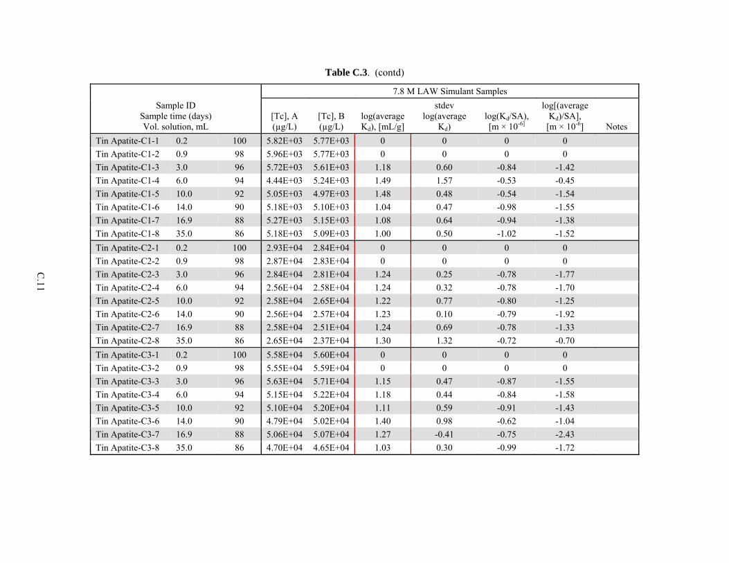
C

.11

Table C.3. (contd)



[Tc], A (µg/L)

[Tc], B (µg/L)


stdev log(average

Kd) log(Kd/SA), [m × 10-6]


[m × 10-6] Notes

Tin Apatite-C1-1 0.2 100 5.82E+03 5.77E+03 0 0 0 0

Tin Apatite-C1-2 0.9 98 5.96E+03 5.77E+03 0 0 0 0

Tin Apatite-C1-3 3.0 96 5.72E+03 5.61E+03 1.18 0.60 -0.84 -1.42

Tin Apatite-C1-4 6.0 94 4.44E+03 5.24E+03 1.49 1.57 -0.53 -0.45

Tin Apatite-C1-5 10.0 92 5.05E+03 4.97E+03 1.48 0.48 -0.54 -1.54

Tin Apatite-C1-6 14.0 90 5.18E+03 5.10E+03 1.04 0.47 -0.98 -1.55

Tin Apatite-C1-7 16.9 88 5.27E+03 5.15E+03 1.08 0.64 -0.94 -1.38

Tin Apatite-C1-8 35.0 86 5.18E+03 5.09E+03 1.00 0.50 -1.02 -1.52

Tin Apatite-C2-1 0.2 100 2.93E+04 2.84E+04 0 0 0 0

Tin Apatite-C2-2 0.9 98 2.87E+04 2.83E+04 0 0 0 0

Tin Apatite-C2-3 3.0 96 2.84E+04 2.81E+04 1.24 0.25 -0.78 -1.77

Tin Apatite-C2-4 6.0 94 2.56E+04 2.58E+04 1.24 0.32 -0.78 -1.70

Tin Apatite-C2-5 10.0 92 2.58E+04 2.65E+04 1.22 0.77 -0.80 -1.25

Tin Apatite-C2-6 14.0 90 2.56E+04 2.57E+04 1.23 0.10 -0.79 -1.92

Tin Apatite-C2-7 16.9 88 2.58E+04 2.51E+04 1.24 0.69 -0.78 -1.33

Tin Apatite-C2-8 35.0 86 2.65E+04 2.37E+04 1.30 1.32 -0.72 -0.70

Tin Apatite-C3-1 0.2 100 5.58E+04 5.60E+04 0 0 0 0

Tin Apatite-C3-2 0.9 98 5.55E+04 5.59E+04 0 0 0 0

Tin Apatite-C3-3 3.0 96 5.63E+04 5.71E+04 1.15 0.47 -0.87 -1.55

Tin Apatite-C3-4 6.0 94 5.15E+04 5.22E+04 1.18 0.44 -0.84 -1.58

Tin Apatite-C3-5 10.0 92 5.10E+04 5.20E+04 1.11 0.59 -0.91 -1.43

Tin Apatite-C3-6 14.0 90 4.79E+04 5.02E+04 1.40 0.98 -0.62 -1.04

Tin Apatite-C3-7 16.9 88 5.06E+04 5.07E+04 1.27 -0.41 -0.75 -2.43

Tin Apatite-C3-8 35.0 86 4.70E+04 4.65E+04 1.03 0.30 -0.99 -1.72

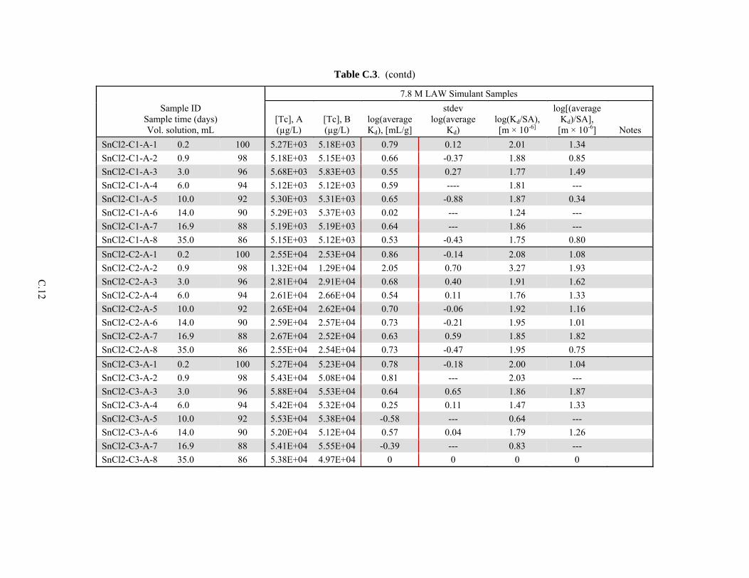
C

.12

Table C.3. (contd)



[Tc], A (µg/L)

[Tc], B (µg/L)


stdev log(average

Kd) log(Kd/SA), [m × 10-6]


[m × 10-6] Notes

SnCl2-C1-A-1 0.2 100 5.27E+03 5.18E+03 0.79 0.12 2.01 1.34

SnCl2-C1-A-2 0.9 98 5.18E+03 5.15E+03 0.66 -0.37 1.88 0.85

SnCl2-C1-A-3 3.0 96 5.68E+03 5.83E+03 0.55 0.27 1.77 1.49

SnCl2-C1-A-4 6.0 94 5.12E+03 5.12E+03 0.59 ---- 1.81 ---

SnCl2-C1-A-5 10.0 92 5.30E+03 5.31E+03 0.65 -0.88 1.87 0.34

SnCl2-C1-A-6 14.0 90 5.29E+03 5.37E+03 0.02 --- 1.24 ---

SnCl2-C1-A-7 16.9 88 5.19E+03 5.19E+03 0.64 --- 1.86 ---

SnCl2-C1-A-8 35.0 86 5.15E+03 5.12E+03 0.53 -0.43 1.75 0.80

SnCl2-C2-A-1 0.2 100 2.55E+04 2.53E+04 0.86 -0.14 2.08 1.08

SnCl2-C2-A-2 0.9 98 1.32E+04 1.29E+04 2.05 0.70 3.27 1.93

SnCl2-C2-A-3 3.0 96 2.81E+04 2.91E+04 0.68 0.40 1.91 1.62

SnCl2-C2-A-4 6.0 94 2.61E+04 2.66E+04 0.54 0.11 1.76 1.33

SnCl2-C2-A-5 10.0 92 2.65E+04 2.62E+04 0.70 -0.06 1.92 1.16

SnCl2-C2-A-6 14.0 90 2.59E+04 2.57E+04 0.73 -0.21 1.95 1.01

SnCl2-C2-A-7 16.9 88 2.67E+04 2.52E+04 0.63 0.59 1.85 1.82

SnCl2-C2-A-8 35.0 86 2.55E+04 2.54E+04 0.73 -0.47 1.95 0.75

SnCl2-C3-A-1 0.2 100 5.27E+04 5.23E+04 0.78 -0.18 2.00 1.04

SnCl2-C3-A-2 0.9 98 5.43E+04 5.08E+04 0.81 --- 2.03 ---

SnCl2-C3-A-3 3.0 96 5.88E+04 5.53E+04 0.64 0.65 1.86 1.87

SnCl2-C3-A-4 6.0 94 5.42E+04 5.32E+04 0.25 0.11 1.47 1.33

SnCl2-C3-A-5 10.0 92 5.53E+04 5.38E+04 -0.58 --- 0.64 ---

SnCl2-C3-A-6 14.0 90 5.20E+04 5.12E+04 0.57 0.04 1.79 1.26

SnCl2-C3-A-7 16.9 88 5.41E+04 5.55E+04 -0.39 --- 0.83 ---

SnCl2-C3-A-8 35.0 86 5.38E+04 4.97E+04 0 0 0 0

C

.13

Table C.3. (contd)



[Tc], A (µg/L)

[Tc], B (µg/L)


stdev log(average

Kd) log(Kd/SA), [m × 10-6]


[m × 10-6] Notes




Note: These blank values were obtained in conjunction with the values given for BFS 1, BFS 2, Tin apatite, and SnCl2 for the experiments conducted in the 7.8 M Na LAW simulant.

C

.14

Table C.4.



[Tc], A (µg/L)

[Tc], B (µg/L)


stdev log(average

Kd) log(Kd/SA), [m × 10-6]


[m × 10-6] Notes

Nano Sn P-C3-1 0.2 100 5.37E+04 5.42E+04 0.56 -0.18 -0.93 ---

Nano Sn P-C3-2 0.9 98 5.28E+04 5.15E+04 0.60 0.27 -0.90 -1.26

Nano Sn P-C3-3 3.0 96 4.63E+04 5.20E+04 0.83 0.93 -0.76 -0.71

Nano Sn P-C3-4 6.0 94 5.12E+04 5.06E+04 0.80 -0.05 -0.78 ---

Nano Sn P-C3-5 10.0 92 5.39E+04 5.25E+04 0.23 --- -1.32 ---

Nano Sn P-C3-6 14.0 90 5.44E+04 5.24E+04 0.42 --- -1.06 ---

Nano Sn P-C3-7 16.9 88 5.32E+04 5.49E+04 0.24 0.30 -1.30 -1.20

Nano Sn P-C3-8 35.0 86 4.91E+04 5.08E+04 0 0 0 0

KMS-C3-1 0.2 100 3.88E+03 3.62E+03 3.17 1.75 -0.21 -0.46

KMS-C3-2 0.9 98 9.00E+02 9.81E+02 3.77 2.65 -0.13 -0.28

KMS-C3-3 3.0 96 1.22E+03 1.32E+03 3.61 2.47 -0.15 -0.32

KMS-C3-4 6.0 94 1.68E+03 1.10E+03 3.60 3.06 -0.15 -0.22

KMS-C3-5 10.0 92 2.30E+03 1.22E+03 3.50 3.14 -0.16 -0.21

KMS-C3-6 14.0 90 2.32E+03 3.45E+03 3.25 2.73 -0.20 -0.27

KMS-C3-7 16.9 88 1.17E+03 1.69E+03 3.56 3.00 -0.16 -0.23

KMS-C3-8 35.0 86 4.25E+02 4.46E+02 4.00 2.69 -0.10 -0.28

Sn-HA-C3-1 0.2 100 5.36E+04 5.22E+04 0.75 0.30 -2.03 -2.43

Sn-HA-C3-2 0.9 98 5.26E+04 5.21E+04 0.55 -0.15 -2.17 ---

Sn-HA-C3-3 3.0 96 5.19E+04 5.08E+04 0.31 0.17 -2.41 -2.67

Sn-HA-C3-4 6.0 94 4.64E+04 4.65E+04 1.19 -1.24 -1.83 ---

Sn-HA-C3-5 10.0 92 4.28E+04 4.28E+04 1.36 -0.80 -1.78 ---

Sn-HA-C3-6 14.0 90 3.61E+04 3.34E+04 1.69 0.90 -1.68 -1.95

Sn-HA-C3-7 16.9 88 2.87E+04 2.45E+04 1.98 1.32 -1.61 -1.79

Sn-HA-C3-8 35.0 86 4.71E+04 4.95E+04 0.49 --- -2.22 ---

C

.15

Table C.4. (contd)



[Tc], A (µg/L)

[Tc], B (µg/L)


stdev log(average

Kd) log(Kd/SA), [m × 10-6]


[m × 10-6] Notes

BFS 1 1:10-C3-1 0.2 100 5.24E+04 5.29E+04 -0.21 -1.15 --- ---

BFS 1 1:10-C3-2 0.9 98 4.91E+04 5.12E+04 -0.09 -0.50 --- ---

BFS 1 1:10-C3-3 3.0 96 4.93E+04 4.82E+04 -0.13 -0.78 --- ---

BFS 1 1:10-C3-4 6.0 94 4.47E+04 4.34E+04 0.34 -0.61 -0.74 ---

BFS 1 1:10-C3-5 10.0 92 4.44E+04 4.43E+04 0.28 -1.69 -0.83 ---

BFS 1 1:10-C3-6 14.0 90 4.35E+04 4.37E+04 0.33 -1.48 -0.76 ---

BFS 1 1:10-C3-7 16.9 88 4.22E+04 4.37E+04 0.40 -0.56 -0.68 ---

BFS 1 1:10-C3-8 35.0 86 4.18E+04 4.22E+04 0.15 -1.18 -1.11 ---

BLK9-C3-1 0.2 100 5.55E+04 5.63E+04

BLK9-C3-2 0.9 98 5.32E+04 5.53E+04

BLK9-C3-3 3.0 96 5.22E+04 5.27E+04

BLK9-C3-4 6.0 94 5.27E+04 5.58E+04

BLK9-C3-5 10.0 92 5.25E+04 5.44E+04

BLK9-C3-6 14.0 90 5.46E+04 5.32E+04

BLK9-C3-7 16.9 88 5.60E+04 5.42E+04

BLK9-C3-8 35.0 86 4.90E+04 4.86E+04

Note: These blank values were obtained in conjunction with the values given for Nano Sn P, KMS, Sn-HA, and BFS 1 1:10 for the experiments conducted in the 7.8 M Na LAW simulant.

C

.16

Table C.5.


DDI Samples

[Tc], A (µg/L)

[Tc], B (µg/L)


stdev log(average

Kd) log(Kd/SA), [m × 10-6]


[m × 10-6] Notes

LBH-C1-1 0.2 100 1.11E+02 1.14E+02 2.71 1.06 2.11 0.47

LBH-C1-2 1.0 98 3.94E+01 4.58E+01 3.16 2.21 2.57 1.62

LBH-C1-3 3.1 96 2.61E+01 2.87E+01 3.35 2.20 2.76 1.61

LBH-C1-4 6.0 94 1.96E+01 2.61E+01 3.42 2.73 2.82 2.14

LBH-C1-5 9.0 92 1.67E+01 2.19E+01 3.47 2.76 2.87 2.17

LBH-C1-6 12.0 90 1.58E+01 2.13E+01 3.47 2.80 2.88 2.21

LBH-C1-7 15.0 88 1.68E+01 2.12E+01 3.46 2.69 2.87 2.10

LBH-C1-8 46.0 86 1.62E+01 2.06E+01 3.45 2.67 2.84 2.08

LBH-C2-1 0.2 100 5.84E+02 6.80E+02 2.66 1.78 2.07 1.18

LBH-C2-2 1.0 98 2.65E+02 2.84E+02 3.06 1.79 2.47 1.20

LBH-C2-3 3.1 96 1.70E+02 1.88E+02 3.26 2.14 2.67 1.55

LBH-C2-4 6.0 94 1.27E+02 1.45E+02 3.35 2.34 2.76 1.75

LBH-C2-5 9.0 92 1.10E+02 1.22E+02 3.39 2.28 2.80 1.68

LBH-C2-6 12.0 90 9.76E+01 1.01E+02 3.45 1.85 2.86 1.26

LBH-C2-7 15.0 88 1.03E+02 1.14E+02 3.41 2.28 2.82 1.69

LBH-C2-8 46.0 86 9.12E+01 1.08E+02 3.44 2.54 2.85 1.94

LBH-C3-1 0.2 100 1.69E+03 1.53E+03 2.54 1.57 1.96 0.97

LBH-C3-2 1.0 98 6.91E+02 6.59E+02 2.98 1.69 2.39 1.10

LBH-C3-3 3.1 96 4.38E+02 4.17E+02 3.17 1.88 2.58 1.29

LBH-C3-4 6.0 94 3.13E+02 2.99E+02 3.29 1.97 2.70 1.38

LBH-C3-5 9.0 92 2.82E+02 2.56E+02 3.31 2.24 2.72 1.65

LBH-C3-6 12.0 90 2.70E+02 2.54E+02 3.32 2.09 2.73 1.50

LBH-C3-7 15.0 88 2.63E+02 2.45E+02 3.34 2.16 2.75 1.57

LBH-C3-8 46.0 86 2.32E+02 2.21E+02 3.41 2.11 2.82 1.52

C

.17

Table C.5. (contd)


DDI Samples

[Tc], A (µg/L)

[Tc], B (µg/L)


stdev log(average

Kd) log(Kd/SA), [m × 10-6]


[m × 10-6] Notes

Argentite-C1-1 0.2 100 6.00E+02 5.61E+02 1.26 0.77 1.57 1.07

Argentite-C1-2 1.0 98 4.53E+02 4.51E+02 1.67 -0.10 1.98 0.20

Argentite-C1-3 3.1 96 4.25E+02 0.00E+00 0 0 0 0

Argentite-C1-4 6.0 94 4.16E+02 3.66E+02 1.79 1.17 2.10 1.47

Argentite-C1-5 9.0 92 3.75E+02 3.58E+02 1.81 0.75 2.11 1.05

Argentite-C1-6 12.0 90 3.76E+02 3.75E+02 1.76 -0.16 2.06 0.14

Argentite-C1-7 15.0 88 3.71E+02 3.72E+02 1.80 -0.78 2.11 -0.48

Argentite-C1-8 46.0 86 3.42E+02 3.25E+02 1.86 0.78 2.13 1.08

Argentite-C2-1 0.2 100 3.03E+03 3.22E+03 1.05 0.69 1.36 0.99

Argentite-C2-2 1.0 98 2.97E+03 2.94E+03 1.25 -0.15 1.56 0.15

Argentite-C2-3 3.1 96 2.84E+03 2.83E+03 1.40 -0.90 1.71 -0.60

Argentite-C2-4 6.0 94 2.68E+03 2.72E+03 1.38 0.15 1.68 0.45

Argentite-C2-5 9.0 92 2.57E+03 2.58E+03 1.37 -0.32 1.67 -0.02

Argentite-C2-6 12.0 90 2.55E+03 2.53E+03 1.37 -0.33 1.67 -0.03

Argentite-C2-7 15.0 88 2.63E+03 2.57E+03 1.36 0.22 1.67 0.52

Argentite-C2-8 46.0 86 2.38E+03 2.45E+03 1.49 0.42 1.80 0.72

Argentite-C3-1 0.2 100 6.59E+03 6.65E+03 0.96 -0.11 1.26 0.19

Argentite-C3-2 1.0 98 6.27E+03 6.12E+03 1.19 0.27 1.49 0.57

Argentite-C3-3 3.0 96 6.27E+03 6.21E+03 1.04 -0.18 1.34 0.12

Argentite-C3-4 6.0 94 5.91E+03 5.71E+03 1.14 0.40 1.44 0.71

Argentite-C3-5 9.0 92 5.67E+03 5.90E+03 0.83 0.45 1.13 0.75

Argentite-C3-6 12.0 90 5.40E+03 5.71E+03 1.10 0.62 1.41 0.92

Argentite-C3-7 15.0 88 5.36E+03 5.39E+03 1.29 -0.25 1.60 0.05

Argentite-C3-8 46.0 86 5.68E+03 5.42E+03 1.35 0.54 1.65 0.84

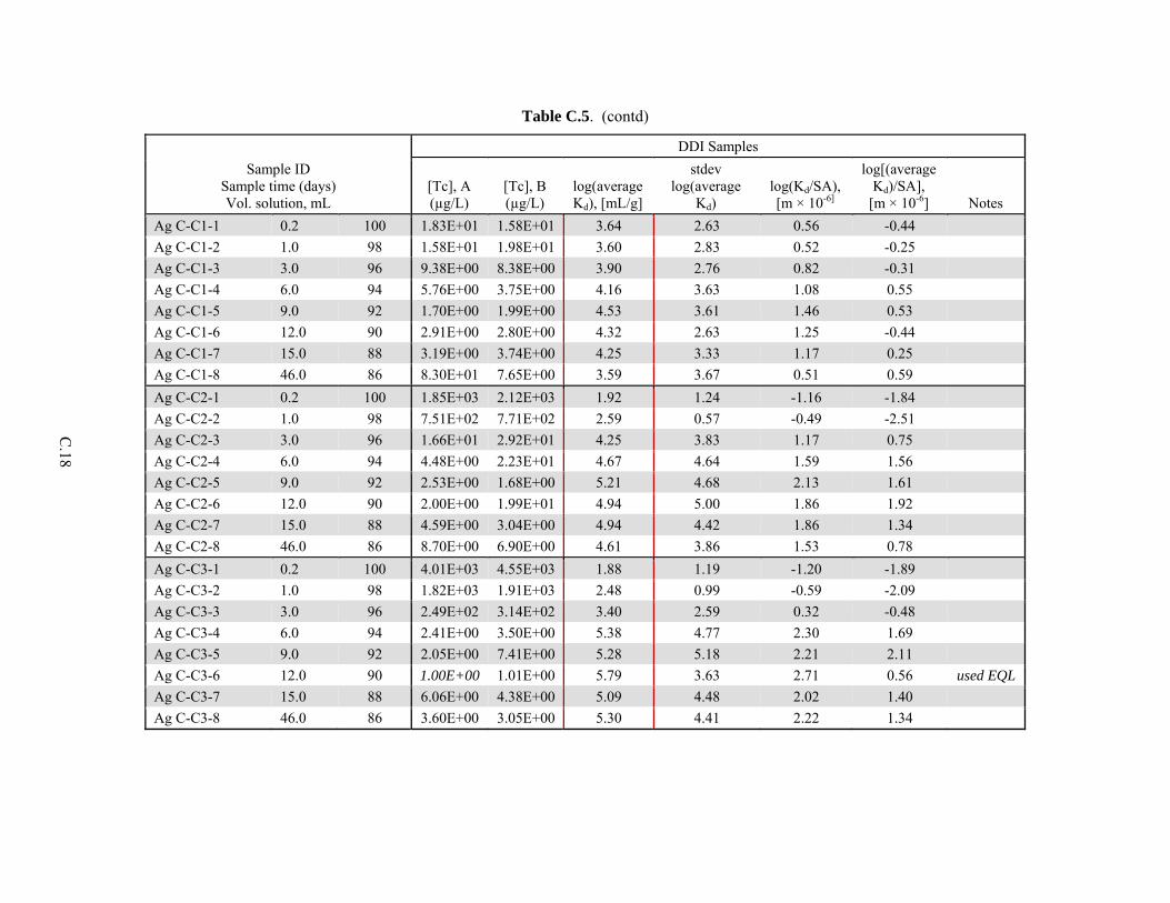
C

.18

Table C.5. (contd)


DDI Samples

[Tc], A (µg/L)

[Tc], B (µg/L)


stdev log(average

Kd) log(Kd/SA), [m × 10-6]


[m × 10-6] Notes

Ag C-C1-1 0.2 100 1.83E+01 1.58E+01 3.64 2.63 0.56 -0.44

Ag C-C1-2 1.0 98 1.58E+01 1.98E+01 3.60 2.83 0.52 -0.25

Ag C-C1-3 3.0 96 9.38E+00 8.38E+00 3.90 2.76 0.82 -0.31

Ag C-C1-4 6.0 94 5.76E+00 3.75E+00 4.16 3.63 1.08 0.55

Ag C-C1-5 9.0 92 1.70E+00 1.99E+00 4.53 3.61 1.46 0.53

Ag C-C1-6 12.0 90 2.91E+00 2.80E+00 4.32 2.63 1.25 -0.44

Ag C-C1-7 15.0 88 3.19E+00 3.74E+00 4.25 3.33 1.17 0.25

Ag C-C1-8 46.0 86 8.30E+01 7.65E+00 3.59 3.67 0.51 0.59

Ag C-C2-1 0.2 100 1.85E+03 2.12E+03 1.92 1.24 -1.16 -1.84

Ag C-C2-2 1.0 98 7.51E+02 7.71E+02 2.59 0.57 -0.49 -2.51

Ag C-C2-3 3.0 96 1.66E+01 2.92E+01 4.25 3.83 1.17 0.75

Ag C-C2-4 6.0 94 4.48E+00 2.23E+01 4.67 4.64 1.59 1.56

Ag C-C2-5 9.0 92 2.53E+00 1.68E+00 5.21 4.68 2.13 1.61

Ag C-C2-6 12.0 90 2.00E+00 1.99E+01 4.94 5.00 1.86 1.92

Ag C-C2-7 15.0 88 4.59E+00 3.04E+00 4.94 4.42 1.86 1.34

Ag C-C2-8 46.0 86 8.70E+00 6.90E+00 4.61 3.86 1.53 0.78

Ag C-C3-1 0.2 100 4.01E+03 4.55E+03 1.88 1.19 -1.20 -1.89

Ag C-C3-2 1.0 98 1.82E+03 1.91E+03 2.48 0.99 -0.59 -2.09

Ag C-C3-3 3.0 96 2.49E+02 3.14E+02 3.40 2.59 0.32 -0.48

Ag C-C3-4 6.0 94 2.41E+00 3.50E+00 5.38 4.77 2.30 1.69

Ag C-C3-5 9.0 92 2.05E+00 7.41E+00 5.28 5.18 2.21 2.11

Ag C-C3-6 12.0 90 1.00E+00 1.01E+00 5.79 3.63 2.71 0.56 used EQL

Ag C-C3-7 15.0 88 6.06E+00 4.38E+00 5.09 4.48 2.02 1.40

Ag C-C3-8 46.0 86 3.60E+00 3.05E+00 5.30 4.41 2.22 1.34

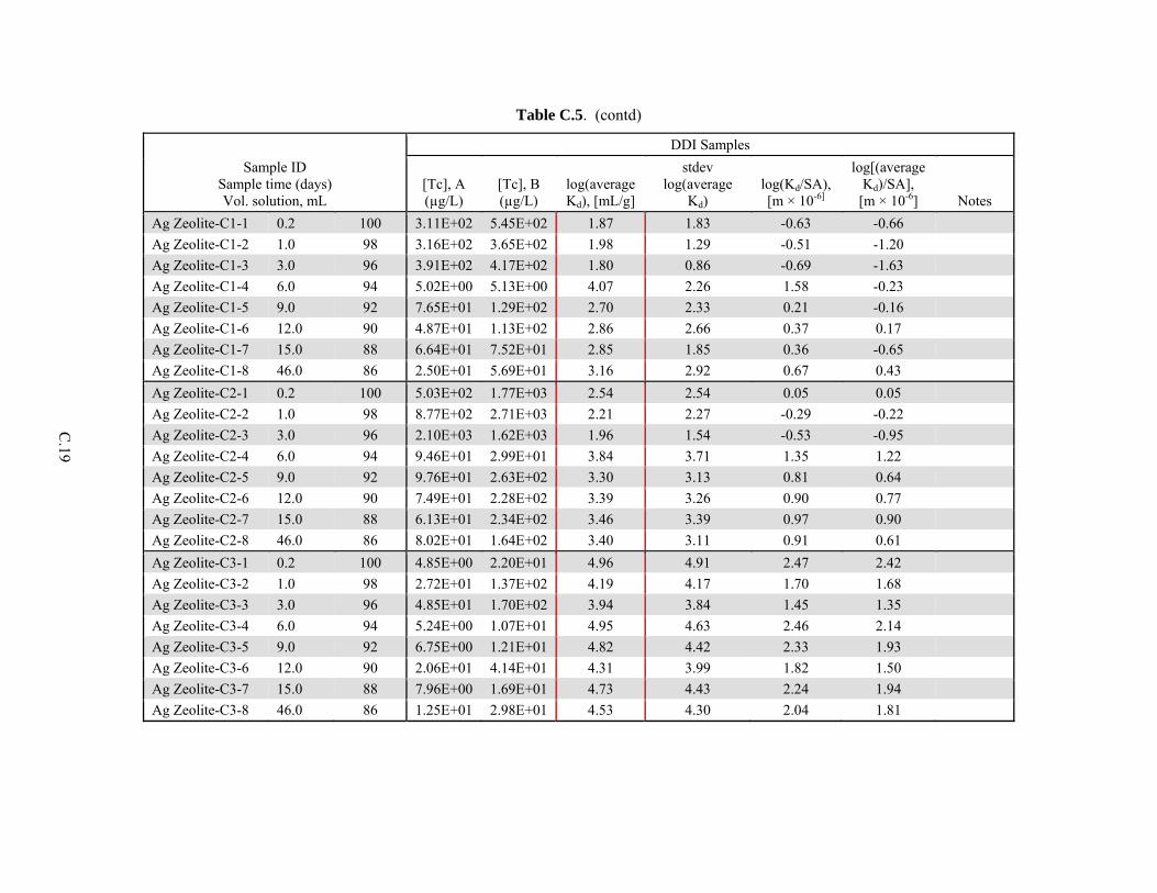
C

.19

Table C.5. (contd)


DDI Samples

[Tc], A (µg/L)

[Tc], B (µg/L)


stdev log(average

Kd) log(Kd/SA), [m × 10-6]


[m × 10-6] Notes

Ag Zeolite-C1-1 0.2 100 3.11E+02 5.45E+02 1.87 1.83 -0.63 -0.66

Ag Zeolite-C1-2 1.0 98 3.16E+02 3.65E+02 1.98 1.29 -0.51 -1.20

Ag Zeolite-C1-3 3.0 96 3.91E+02 4.17E+02 1.80 0.86 -0.69 -1.63

Ag Zeolite-C1-4 6.0 94 5.02E+00 5.13E+00 4.07 2.26 1.58 -0.23

Ag Zeolite-C1-5 9.0 92 7.65E+01 1.29E+02 2.70 2.33 0.21 -0.16

Ag Zeolite-C1-6 12.0 90 4.87E+01 1.13E+02 2.86 2.66 0.37 0.17

Ag Zeolite-C1-7 15.0 88 6.64E+01 7.52E+01 2.85 1.85 0.36 -0.65

Ag Zeolite-C1-8 46.0 86 2.50E+01 5.69E+01 3.16 2.92 0.67 0.43

Ag Zeolite-C2-1 0.2 100 5.03E+02 1.77E+03 2.54 2.54 0.05 0.05

Ag Zeolite-C2-2 1.0 98 8.77E+02 2.71E+03 2.21 2.27 -0.29 -0.22

Ag Zeolite-C2-3 3.0 96 2.10E+03 1.62E+03 1.96 1.54 -0.53 -0.95

Ag Zeolite-C2-4 6.0 94 9.46E+01 2.99E+01 3.84 3.71 1.35 1.22

Ag Zeolite-C2-5 9.0 92 9.76E+01 2.63E+02 3.30 3.13 0.81 0.64

Ag Zeolite-C2-6 12.0 90 7.49E+01 2.28E+02 3.39 3.26 0.90 0.77

Ag Zeolite-C2-7 15.0 88 6.13E+01 2.34E+02 3.46 3.39 0.97 0.90

Ag Zeolite-C2-8 46.0 86 8.02E+01 1.64E+02 3.40 3.11 0.91 0.61

Ag Zeolite-C3-1 0.2 100 4.85E+00 2.20E+01 4.96 4.91 2.47 2.42

Ag Zeolite-C3-2 1.0 98 2.72E+01 1.37E+02 4.19 4.17 1.70 1.68

Ag Zeolite-C3-3 3.0 96 4.85E+01 1.70E+02 3.94 3.84 1.45 1.35

Ag Zeolite-C3-4 6.0 94 5.24E+00 1.07E+01 4.95 4.63 2.46 2.14

Ag Zeolite-C3-5 9.0 92 6.75E+00 1.21E+01 4.82 4.42 2.33 1.93

Ag Zeolite-C3-6 12.0 90 2.06E+01 4.14E+01 4.31 3.99 1.82 1.50

Ag Zeolite-C3-7 15.0 88 7.96E+00 1.69E+01 4.73 4.43 2.24 1.94

Ag Zeolite-C3-8 46.0 86 1.25E+01 2.98E+01 4.53 4.30 2.04 1.81

C

.20

Table C.5. (contd)


DDI Samples

[Tc], A (µg/L)

[Tc], B (µg/L)


stdev log(average

Kd) log(Kd/SA), [m × 10-6]


[m × 10-6] Notes

Syn Arg-C1-1 0.2 100 3.28E+02 4.09E+02 1.95 1.49 1.91 1.44

Syn Arg-C1-2 1.0 98 1.01E+02 1.34E+02 2.67 2.08 2.63 2.04

Syn Arg-C1-3 3.0 96 1.02E+01 1.56E+01 3.71 3.21 3.67 3.17

Syn Arg-C1-4 6.0 94 1.90E+00 1.84E+00 4.51 2.45 4.47 2.40

Syn Arg-C1-5 9.0 92 1.18E+00 1.00E+00 4.72 3.73 4.68 3.69 used EQL




Syn Arg-C2-1 0.2 100 2.39E+03 2.27E+03 1.69 0.76 1.65 0.72

Syn Arg-C2-2 1.0 98 7.94E+02 9.96E+02 2.46 1.78 2.42 1.73

Syn Arg-C2-3 3.0 96 1.62E+02 1.98E+02 3.26 2.41 3.22 2.37

Syn Arg-C2-4 6.0 94 7.39E+00 8.58E+00 4.60 3.59 4.56 3.55

Syn Arg-C2-5 9.0 92 1.91E+00 1.47E+00 5.25 4.53 5.21 4.49




Syn Arg-C3-1 0.2 100 4.30E+03 4.47E+03 1.81 0.66 1.77 0.61

Syn Arg-C3-2 1.0 98 2.78E+03 2.28E+03 2.26 1.59 2.22 1.55

Syn Arg-C3-3 3.0 96 9.04E+02 6.82E+02 2.88 2.23 2.84 2.19

Syn Arg-C3-4 6.0 94 9.61E+01 1.01E+02 3.80 2.35 3.76 2.31

Syn Arg-C3-5 9.0 92 7.47E+00 1.91E+01 4.73 4.52 4.68 4.48

Syn Arg-C3-6 12.0 90 2.09E+00 7.97E+00 5.24 5.15 5.19 5.11

Syn Arg-C3-7 15.0 88 1.10E+00 2.81E+00 5.56 5.36 5.52 5.31

Syn Arg-C3-8 46.0 86 2.50E+00 2.50E+00 5.38 --- 5.34 --- used EQL

C

.21

Table C.5. (contd)


DDI Samples

[Tc], A (µg/L)

[Tc], B (µg/L)


stdev log(average

Kd) log(Kd/SA), [m × 10-6]


[m × 10-6] Notes

I BLK1-C1-1 0.2 100 6.87E+02 6.86E+02 I BLK1-C1-2 1.0 98 6.57E+02 6.81E+02 I BLK1-C1-3 3.0 96 6.71E+02 6.71E+02 I BLK1-C1-4 6.0 94 6.54E+02 6.36E+02 I BLK1-C1-5 9.0 92 6.35E+02 6.08E+02 I BLK1-C1-6 12.0 90 6.05E+02 6.23E+02 I BLK1-C1-7 15.0 88 6.42E+02 6.35E+02 I BLK1-C1-8 46.0 86 6.35E+02 5.92E+02



Note: These blank values were obtained in conjunction with the values given for LBH, Argentite, Ag C, Ag zeolite, and Syn Arge experiments conducted in DDI.

C

.22

Table C.6.



[Tc], A (µg/L)

[Tc], B (µg/L)


stdev log(average

Kd) log(Kd/SA), [m × 10-6]


[m × 10-6] Notes

LBH-C1-1 0.2 100 6.46E+02 6.36E+02 -0.06 --- -0.65 ---

LBH-C1-2 1.0 98 6.16E+02 6.33E+02 0.42 --- -0.17 ---

LBH-C1-3 3.1 96 6.36E+02 6.45E+02 -0.05 --- -0.64 ---

LBH-C1-4 6.0 94 6.30E+02 6.03E+02 0.36 0.48 -0.24 -0.11

LBH-C1-5 9.0 92 6.22E+02 5.91E+02 0.54 0.54 -0.05 -0.05

LBH-C1-6 12.0 90 5.99E+02 6.29E+02 0.40 0.50 -0.19 -0.09

LBH-C1-7 15.0 88 6.34E+02 5.85E+02 0.75 --- 0.16 ---

LBH-C1-8 46.0 86 6.88E+02 5.82E+02 1.01 --- 0.42 ---

LBH-C2-1 0.2 100 3.10E+03 3.20E+03 0.21 0.36 -0.38 -0.23

LBH-C2-2 1.0 98 3.24E+03 3.04E+03 0.70 --- 0.11 ---

LBH-C2-3 3.1 96 3.10E+03 3.05E+03 0.56 0.06 -0.03 -0.53

LBH-C2-4 6.0 94 2.92E+03 3.07E+03 0.78 0.55 0.19 -0.04

LBH-C2-5 9.0 92 3.05E+03 3.15E+03 0.44 --- -0.16 ---

LBH-C2-6 12.0 90 3.13E+03 3.05E+03 -0.05 --- -0.64 ---

LBH-C2-7 15.0 88 3.04E+03 3.05E+03 0 0 0 0

LBH-C2-8 46.0 86 3.31E+03 3.44E+03 0.62 0.39 0.03 -0.20

LBH-C3-1 0.2 100 6.42E+03 6.39E+03 0 0 0 0

LBH-C3-2 1.0 98 6.31E+03 6.18E+03 0.59 0.17 0.00 -0.42

LBH-C3-3 3.1 96 6.21E+03 6.24E+03 -0.63 -0.48 -1.22 -1.07

LBH-C3-4 6.0 94 6.05E+03 6.32E+03 0.52 --- -0.08 ---

LBH-C3-5 9.0 92 6.00E+03 5.99E+03 0.36 -1.02 -0.23 -1.61

LBH-C3-6 12.0 90 6.24E+03 6.05E+03 0.53 0.30 -0.06 -0.29

LBH-C3-7 15.0 88 6.13E+03 5.90E+03 0.66 0.39 0.07 -0.20

LBH-C3-8 46.0 86 6.90E+03 6.70E+03 0 0 0 0

C

.23

Table C.6. (contd)



[Tc], A (µg/L)

[Tc], B (µg/L)


stdev log(average

Kd) log(Kd/SA), [m × 10-6]


[m × 10-6] Notes

Argentite-C1-1 0.2 100 6.49E+02 6.45E+02 0 0 0 0

Argentite-C1-2 1.0 98 6.44E+02 6.03E+02 0.68 0 0.98 0

Argentite-C1-3 3.1 96 6.49E+02 6.75E+02 0 0 0 0

Argentite-C1-4 6.0 94 6.58E+02 6.27E+02 -0.22 0 0.08 0

Argentite-C1-5 9.0 92 6.43E+02 6.23E+02 -0.05 0 0.25 0

Argentite-C1-6 12.0 90 6.37E+02 6.55E+02 0 0 0 0

Argentite-C1-7 15.0 88 6.46E+02 6.48E+02 0 0 0 0

Argentite-C1-8 46.0 86 7.09E+02 7.22E+02 0 0 0 0

Argentite-C2-1 0.2 100 3.22E+03 3.26E+03 0 0 0 0

Argentite-C2-2 1.0 98 3.21E+03 3.19E+03 -0.81 0 -0.51 0

Argentite-C2-3 3.1 96 3.22E+03 3.15E+03 0.09 0 0.39 0

Argentite-C2-4 6.0 94 3.33E+03 3.11E+03 0.36 0 0.66 0

Argentite-C2-5 9.0 92 3.14E+03 3.31E+03 0 0 0 0

Argentite-C2-6 12.0 90 3.10E+03 3.13E+03 0 0 0 0

Argentite-C2-7 15.0 88 3.13E+03 3.17E+03 0 0 0 0

Argentite-C2-8 46.0 86 3.44E+03 3.40E+03 0.46 -0.13 0.76 0.17

Argentite-C3-1 0.2 100 6.49E+03 6.21E+03 0.38 0 0.68 0

Argentite-C3-2 1.0 98 6.47E+03 6.20E+03 0.40 0.48 0.70 0.78

Argentite-C3-3 3.0 96 6.56E+03 6.54E+03 0 0 0 0

Argentite-C3-4 6.0 94 6.38E+03 6.47E+03 0 0 0 0

Argentite-C3-5 9.0 92 6.41E+03 6.26E+03 0 0 0 0

Argentite-C3-6 12.0 90 6.61E+03 6.24E+03 0.29 0 0.59 0

Argentite-C3-7 15.0 88 6.18E+03 6.54E+03 0.31 0 0.62 0

Argentite-C3-8 46.0 86 6.46E+03 6.07E+03 0.55 0 0.85 0

C

.24

Table C.6. (contd)



[Tc], A (µg/L)

[Tc], B (µg/L)


stdev log(average

Kd) log(Kd/SA), [m × 10-6]


[m × 10-6] Notes

Ag C-C1-1 0.2 100 6.23E+02 6.27E+02 0.46 -0.29 -2.61 -3.37

Ag C-C1-2 1.0 98 6.16E+02 5.83E+02 0.78 0.65 -2.30 -2.43

Ag C-C1-3 3.0 96 6.15E+02 6.46E+02 0.67 --- -2.41 ---

Ag C-C1-4 6.0 94 6.26E+02 6.30E+02 -0.31 -0.33 -3.38 -3.41

Ag C-C1-5 9.0 92 5.82E+02 6.07E+02 0.77 0.50 -2.30 -2.57

Ag C-C1-6 12.0 90 6.13E+02 6.36E+02 0.46 --- -2.61 ---

Ag C-C1-7 15.0 88 6.37E+02 6.08E+02 0.35 --- -2.73 ---

Ag C-C1-8 46.0 86 6.34E+02 6.04E+02 0.70 0.53 -2.38 -2.54

Ag C-C2-1 0.2 100 3.16E+03 3.24E+03 0.14 --- -2.93 ---

Ag C-C2-2 1.0 98 3.19E+03 3.03E+03 0.48 0.61 -2.59 -2.47

Ag C-C2-3 3.0 96 2.97E+03 2.97E+03 0.90 -1.25 -2.18 -4.33

Ag C-C2-4 6.0 94 3.13E+03 3.04E+03 0.53 0.35 -2.55 -2.73

Ag C-C2-5 9.0 92 3.11E+03 3.05E+03 0.30 0.16 -2.78 -2.92

Ag C-C2-6 12.0 90 3.18E+03 3.05E+03 -0.01 --- -3.08 ---

Ag C-C2-7 15.0 88 3.33E+03 2.93E+03 0.30 --- -2.78 ---

Ag C-C2-8 46.0 86 3.37E+03 3.42E+03 0.59 0.00 -2.48 -3.08

Ag C-C3-1 0.2 100 6.19E+03 6.28E+03 0.35 0.07 -2.73 -3.01

Ag C-C3-2 1.0 98 6.23E+03 6.12E+03 0.75 0.13 -2.33 -2.95

Ag C-C3-3 3.0 96 6.21E+03 6.41E+03 -0.29 --- -3.36 ---

Ag C-C3-4 6.0 94 6.28E+03 6.05E+03 0.55 --- -2.53 ---

Ag C-C3-5 9.0 92 6.46E+03 6.16E+03 0 0 0 0

Ag C-C3-6 12.0 90 6.30E+03 6.21E+03 0.28 0.00 -2.80 -3.08

Ag C-C3-7 15.0 88 6.39E+03 6.19E+03 0.32 --- -2.76 ---

Ag C-C3-8 46.0 86 6.88E+03 7.18E+03 0 0 0 0

C

.25

Table C.6. (contd)



[Tc], A (µg/L)

[Tc], B (µg/L)


stdev log(average

Kd) log(Kd/SA), [m × 10-6]


[m × 10-6] Notes

Ag Zeolite-C1-1 0.2 100 2.50E+01 2.50E+01 3.39 0 0.90 0 used EQL
























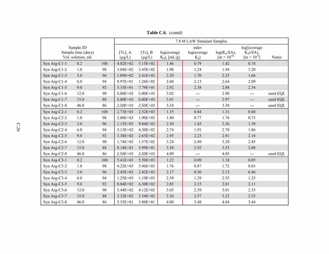
C

.26

Table C.6. (contd)



[Tc], A (µg/L)

[Tc], B (µg/L)


stdev log(average

Kd) log(Kd/SA), [m × 10-6]


[m × 10-6] Notes

Syn Arg-C1-1 0.2 100 4.82E+02 5.15E+02 1.46 0.79 1.42 0.74

Syn Arg-C1-2 1.0 98 3.04E+02 3.45E+02 1.98 1.24 1.94 1.20

Syn Arg-C1-3 3.0 96 1.89E+02 2.41E+02 2.29 1.70 2.25 1.66

Syn Arg-C1-4 6.0 94 8.97E+01 1.26E+02 2.68 2.13 2.64 2.09

Syn Arg-C1-5 9.0 92 5.35E+01 7.79E+01 2.92 2.38 2.88 2.34




Syn Arg-C2-1 0.2 100 2.73E+03 2.52E+03 1.35 0.84 1.31 0.80

Syn Arg-C2-2 1.0 98 2.00E+03 1.90E+03 1.80 0.77 1.76 0.73

Syn Arg-C2-3 3.0 96 1.12E+03 9.84E+02 2.30 1.43 2.26 1.39

Syn Arg-C2-4 6.0 94 5.13E+02 4.30E+02 2.74 1.91 2.70 1.86

Syn Arg-C2-5 9.0 92 3.38E+02 2.65E+02 2.95 2.23 2.91 2.18

Syn Arg-C2-6 12.0 90 1.74E+02 1.37E+02 3.24 2.49 3.20 2.45

Syn Arg-C2-7 15.0 88 8.14E+01 5.99E+01 3.58 2.92 3.53 2.88


Syn Arg-C3-1 0.2 100 5.41E+03 5.50E+03 1.22 0.09 1.18 0.05

Syn Arg-C3-2 1.0 98 4.22E+03 3.96E+03 1.76 0.87 1.72 0.83

Syn Arg-C3-3 3.0 96 2.45E+03 2.42E+03 2.17 0.50 2.13 0.46

Syn Arg-C3-4 6.0 94 1.25E+03 1.19E+03 2.59 1.29 2.55 1.25

Syn Arg-C3-5 9.0 92 8.04E+02 6.30E+02 2.85 2.15 2.81 2.11

Syn Arg-C3-6 12.0 90 5.44E+02 4.12E+02 3.05 2.39 3.01 2.35

Syn Arg-C3-7 15.0 88 3.32E+02 2.54E+02 3.26 2.57 3.22 2.53

Syn Arg-C3-8 46.0 86 5.35E+01 3.80E+01 4.08 3.48 4.04 3.44

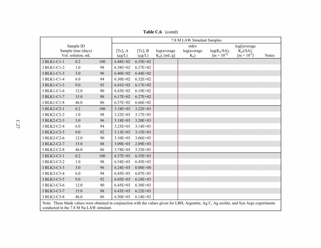
C

.27

Table C.6. (contd)



[Tc], A (µg/L)

[Tc], B (µg/L)


stdev log(average

Kd) log(Kd/SA), [m × 10-6]


[m × 10-6] Notes

I BLK1-C1-1 0.2 100 6.48E+02 6.35E+02

I BLK1-C1-2 1.0 98 6.38E+02 6.27E+02

I BLK1-C1-3 3.0 96 6.40E+02 6.44E+02

I BLK1-C1-4 6.0 94 6.30E+02 6.32E+02

I BLK1-C1-5 9.0 92 6.41E+02 6.17E+02

I BLK1-C1-6 12.0 90 6.43E+02 6.19E+02

I BLK1-C1-7 15.0 88 6.17E+02 6.27E+02

I BLK1-C1-8 46.0 86 6.37E+02 6.66E+02

I BLK2-C2-1 0.2 100 3.18E+03 3.22E+03

I BLK2-C2-2 1.0 98 3.22E+03 3.17E+03

I BLK2-C2-3 3.0 96 3.18E+03 3.20E+03

I BLK2-C2-4 6.0 94 3.23E+03 3.14E+03

I BLK2-C2-5 9.0 92 3.13E+03 3.15E+03

I BLK2-C2-6 12.0 90 3.10E+03 3.06E+03

I BLK2-C2-7 15.0 88 3.09E+03 2.89E+03

I BLK2-C2-8 46.0 86 3.74E+03 3.33E+03

I BLK3-C3-1 0.2 100 6.37E+03 6.35E+03

I BLK3-C3-2 1.0 98 6.54E+03 6.45E+03

I BLK3-C3-3 3.0 96 6.24E+03 0.00E+00

I BLK3-C3-4 6.0 94 6.45E+03 6.07E+03

I BLK3-C3-5 9.0 92 6.05E+03 6.24E+03

I BLK3-C3-6 12.0 90 6.45E+03 6.30E+03

I BLK3-C3-7 15.0 88 6.43E+03 6.22E+03

I BLK3-C3-8 46.0 86 6.50E+03 6.14E+03

Note: These blank values were obtained in conjunction with the values given for LBH, Argentite, Ag C, Ag zeolite, and Syn Arge experiments conducted in the 7.8 M Na LAW simulant.

Table C.7.

Getter Target Species

Blank Set Conc. Solution Rep pH

LBH I A C1 DDI A 6.60 LBH I A C1 DDI B 6.67 LBH I A C1 7.8M A 13.43 LBH I A C1 7.8M B 13.45 LBH I A C2 DDI A 7.39 LBH I A C2 DDI B 7.35 LBH I A C2 7.8M A 13.65 LBH I A C2 7.8M B 13.63 LBH I A C3 DDI A 7.38 LBH I A C3 DDI B 7.23 LBH I A C3 7.8M A 13.65 LBH I A C3 7.8M B 13.63

Argentite I A C1 DDI A 6.38 Argentite I A C1 DDI B 6.41 Argentite I A C1 7.8M A 13.62 Argentite I A C1 7.8M B 13.60 Argentite I A C2 DDI A 6.86 Argentite I A C2 DDI B 6.59 Argentite I A C2 7.8M A 13.60 Argentite I A C2 7.8M B 13.60 Argentite I A C3 DDI A 6.91 Argentite I A C3 DDI B 6.50 Argentite I A C3 7.8M A 13.57 Argentite I A C3 7.8M B 13.58

Ag C I A C1 DDI A 6.93 Ag C I A C1 DDI B 6.93 Ag C I A C1 7.8M A 13.59 Ag C I A C1 7.8M B 13.59 Ag C I A C2 DDI A 7.43 Ag C I A C2 DDI B 7.55 Ag C I A C2 7.8M A 13.61 Ag C I A C2 7.8M B 13.61 Ag C I A C3 DDI A 7.81 Ag C I A C3 DDI B 7.55 Ag C I A C3 7.8M A 13.69 Ag C I A C3 7.8M B 13.65

Table C.7. (contd)


Blank Set Conc. Solution Rep pH

Ag Zeolite I A C1 DDI A 9.86 Ag Zeolite I A C1 DDI B 9.81 Ag Zeolite I A C1 7.8M A 13.63 Ag Zeolite I A C1 7.8M B 13.55 Ag Zeolite I A C2 DDI A 9.72 Ag Zeolite I A C2 DDI B 9.79 Ag Zeolite I A C2 7.8M A 13.56 Ag Zeolite I A C2 7.8M B 13.54 Ag Zeolite I A C3 DDI A 9.83 Ag Zeolite I A C3 DDI B 9.91 Ag Zeolite I A C3 7.8M A 13.53 Ag Zeolite I A C3 7.8M B 13.52

Syn Arg I A C1 DDI A 7.62 Syn Arg I A C1 DDI B 7.71 Syn Arg I A C1 7.8M A 13.50 Syn Arg I A C1 7.8M B 13.50 Syn Arg I A C2 DDI A 7.97 Syn Arg I A C2 DDI B 8.03 Syn Arg I A C2 7.8M A 13.49 Syn Arg I A C2 7.8M B 13.48 Syn Arg I A C3 DDI A 8.67 Syn Arg I A C3 DDI B 8.65 Syn Arg I A C3 7.8M A 13.48 Syn Arg I A C3 7.8M B 13.48

I BLK1 I A C1 DDI A 7.07 I BLK1 I A C1 DDI B 7.16 I BLK4 I A C1 7.8M A 13.58 I BLK4 I A C1 7.8M B 13.57 I BLK2 I A C2 DDI A 7.28 I BLK2 I A C2 DDI B 7.44 I BLK5 I A C2 7.8M A 13.56 I BLK5 I A C2 7.8M B 13.54 I BLK3 I A C3 DDI A 7.96 I BLK3 I A C3 DDI B 7.74 I BLK6 I A C3 7.8M A 13.53 I BLK6 I A C3 7.8M B 13.53

Table C.8.


Blank Set Conc. Solution Rep pH Notes

BFS 1 Tc B C1 DDI A 12.16 BFS 1 Tc B C1 DDI B 12.12 BFS 1 Tc B C1 7.8M A 13.48 BFS 1 Tc B C1 7.8M B 13.65 BFS 1 Tc B C2 DDI A 12.12 BFS 1 Tc B C2 DDI B 12.09 BFS 1 Tc B C2 7.8M A 13.66 BFS 1 Tc B C2 7.8M B 13.70 BFS 1 Tc B C3 DDI A 12.10 BFS 1 Tc B C3 DDI B 12.05 BFS 1 Tc B C3 7.8M A 13.77 BFS 1 Tc B C3 7.8M B 13.80

BFS 2 Tc B C1 DDI A 12.20 BFS 2 Tc B C1 DDI B 12.23 BFS 2 Tc B C1 7.8M A 13.61 BFS 2 Tc B C1 7.8M B 13.60 BFS 2 Tc B C2 DDI A 12.14 (a) BFS 2 Tc B C2 DDI B 12.12 (a) BFS 2 Tc B C2 7.8M A 13.73 BFS 2 Tc B C2 7.8M B 13.74 BFS 2 Tc B C3 DDI A 12.20 BFS 2 Tc B C3 DDI B 12.19 BFS 2 Tc B C3 7.8M A 13.81 BFS 2 Tc B C3 7.8M B 13.80

Tin Apatite Tc B C1 DDI A 7.93 Tin Apatite Tc B C1 DDI B 7.79 Tin Apatite Tc B C1 7.8M A 13.85 Tin Apatite Tc B C1 7.8M B 13.88 Tin Apatite Tc B C2 DDI A 7.83 (a) Tin Apatite Tc B C2 DDI B 7.78 (a) Tin Apatite Tc B C2 7.8M A 13.77 Tin Apatite Tc B C2 7.8M B 13.77 Tin Apatite Tc B C3 DDI A 8.02 Tin Apatite Tc B C3 DDI B 7.88 Tin Apatite Tc B C3 7.8M A 13.82 Tin Apatite Tc B C3 7.8M B 13.81

(a) Calibration check did not pass. (b) Calibration passed but a pH 2 buffer was not available so calibration was checked with a

pH 4 buffer. (c) Checked with two DDIfferent pH 13 buffers. For calibration check and end check, one

passed and the other DDId not.

Table C.9.



SnCl2 Tc B C1 DDI A 1.64 (b) SnCl2 Tc B C1 DDI B 1.58 (b) SnCl2 Tc B C1 7.8M A 13.66 SnCl2 Tc B C1 7.8M B 13.84 SnCl2 Tc B C2 DDI A 1.54 (b) SnCl2 Tc B C2 DDI B 1.53 (b) SnCl2 Tc B C2 7.8M A 13.73 SnCl2 Tc B C2 7.8M B 13.75 SnCl2 Tc B C3 DDI A 1.54 (b) SnCl2 Tc B C3 DDI B 1.56 (b) SnCl2 Tc B C3 7.8M A 13.80 SnCl2 Tc B C3 7.8M B 13.78

BLK1 Tc B C1 DDI A 8.72 BLK1 Tc B C1 DDI B 8.74 BLK2 Tc B C2 DDI A 9.83 BLK2 Tc B C2 DDI B 9.27 BLK3 Tc B C3 DDI A 8.71 BLK3 Tc B C3 DDI B 8.66 BLK4 Tc B C1 7.8M A 13.87 BLK4 Tc B C1 7.8M B 13.89 BLK5 Tc B C2 7.8M A 13.76 BLK5 Tc B C2 7.8M B 13.06 BLK6 Tc B C3 7.8M A 13.75 BLK6 Tc B C3 7.8M B 13.75

Nano Sn P Tc C C3 DDI A 4.15 Nano Sn P Tc C C3 DDI B 4.10 Nano Sn P Tc C C3 7.8M A 13.73 (c) Nano Sn P Tc C C3 7.8M B 13.73 (c)

KMS Tc C C3 DDI A 10.28 KMS Tc C C3 DDI B 10.25 KMS Tc C C3 7.8M A 13.63 (c) KMS Tc C C3 7.8M B 13.68 (c) Sn-HA Tc C C3 DDI A 9.30 Sn-HA Tc C C3 DDI B 8.71 Sn-HA Tc C C3 7.8M A 13.70 (c) Sn-HA Tc C C3 7.8M B 13.71 (c) (a) Calibration check did not pass. (b) Calibration passed but a pH 2 buffer was not available so calibration was checked with a

pH 4 buffer. (c) Checked with 2 DDIfferent pH 13 buffers. For calibration check and end check, one

passed and the other DDId not.

Table C.10.



BFS 1 1:10 Tc C C3 DDI B 12.36 BFS 1 1:10 Tc C C3 7.8M A 13.74 (c)BFS 1 1:10 Tc C C3 7.8M B 13.72 (c)

BLK11 Tc C C3 DDI A 9.62 BLK12 Tc C C3 DDI B 9.29 BLK17 Tc C C3 7.8M A 13.70 (c)BLK18 Tc C C3 7.8M B 13.67 (c)

(a) Calibration check did not pass. (b) Calibration passed but a pH 2 buffer was not available so calibration was checked with a pH 4

buffer. (c) Checked with 2 DDIfferent pH 13 buffers. For calibration check and end check, one passed and the other DDId not.

Technetium and Iodine Getters to Improve Cast Stone Performance

Documents

Transcript of Technetium and Iodine Getters to Improve Cast Stone Performance